Embed Size (px)
Citation preview

Master thesis in Sustainable Development 302
Examensarbete i Hållbar utveckling
Photovoltaic power potential on
Gotland: A comparison with load, wind
power and power export possibilities
Emil Zaar
DEPARTMENT OF
EARTH SCIENCES
I N S T I T U T I O N E N F Ö R
G E O V E T E N S K A P E R


Master thesis in Sustainable Development 302
Examensarbete i Hållbar utveckling
Photovoltaic power potential on Gotland: A
comparison with load, wind power and power
export possibilities
Emil Zaar
Supervisor: Rasmus Luthander
Evaluator: Joakim Munkhammar

Copyright © Emil Zaar and the Department of Earth Sciences, Uppsala University
Published at Department of Earth Sciences, Uppsala University (www.geo.uu.se), Uppsala, 2016

II
Content 1. Introduction .......................................................................................................................... 1
1.1. Aims and objectives ........................................................................................................ 2
1.1.1. Research Questions .................................................................................................. 2
1.2. Background ..................................................................................................................... 3
1.2.1. Environmental goals and Future scenarios ............................................................... 6
1.3. Sustainable development and research mode .................................................................. 7
1.3.1. Previous Photovoltaic power potential studies on Gotland ...................................... 8
1.4. Delimitations ................................................................................................................... 9
1.4.1. Solar PV Potential method ....................................................................................... 9
2. Theory ................................................................................................................................. 10
2.1. Solar Radiation .............................................................................................................. 10
2.1.1. Tilt, Angle, Latitude ............................................................................................... 10
2.2. Photovoltaic Cells.......................................................................................................... 10
2.2.1. Inverter ................................................................................................................... 11
2.3. Types of Photovoltaic Cells .......................................................................................... 11
2.3.1. Polycrystalline ........................................................................................................ 11
2.3.2. Monocrystalline ...................................................................................................... 11
2.3.3. Thin-Film ............................................................................................................... 11
2.4. Wind speed and the power of the wind ......................................................................... 11
2.5. Electrical grid ................................................................................................................ 12
2.5.1. National grid ........................................................................................................... 12
2.5.2. Regional grid .......................................................................................................... 12
2.5.3. Distribution grid ..................................................................................................... 12
2.5.4. Price areas .............................................................................................................. 13
2.6. Distributed generation ................................................................................................... 13
2.7. Electrical grid on Gotland ............................................................................................. 13
2.8. Microgeneration ............................................................................................................ 14
2.9. Electric load ................................................................................................................... 14
3. Methods and Data .............................................................................................................. 16
3.1. Solar radiation ............................................................................................................... 16

III
3.2. Building types and building area ................................................................................... 16
3.2.1. Roof Shape and angle ............................................................................................. 17
3.3. Building categories ........................................................................................................ 17
3.3.1. Roof Type ............................................................................................................... 18
3.3.2. Roof area ................................................................................................................ 18
3.4. Azimuth angle ............................................................................................................... 18
3.4.1. Azimuth angles impact on a tilted surface respectively flat surface ...................... 19
3.4.2. Buildings azimuth orientation ................................................................................ 22
3.4.3. Available area for PV arrays on a flat roofs ........................................................... 22
3.5. Additional limiting factors ............................................................................................ 23
3.5.1. Shading ................................................................................................................... 23
3.5.2. Snow and soiling losses .......................................................................................... 24
3.6. Total reductions ............................................................................................................. 24
3.7. Data and building categorization ................................................................................... 24
3.8. Load data and electric energy consumption .................................................................. 26
3.9. Wind power simulation and data ................................................................................... 26
3.10. Hourly comparison ...................................................................................................... 28
4. Results ................................................................................................................................. 29
4.1. Summary of the PV power potential 2010-2012 ........................................................... 29
4.2. Wind Power ................................................................................................................... 31
4.3. Load and consumption data on average year ................................................................ 32
4.4. Monthly electric consumption and production .............................................................. 33
4.5. Potential PV power capacity with the current and prospective submarine power cable
.............................................................................................................................................. 35
5. Discussion ........................................................................................................................ 37
6. Future Work ......................................................................................................................... 38
7. Conclusion ........................................................................................................................... 39
8. Acknowledgements ............................................................................................................. 39
9. References ........................................................................................................................... 40
9.1. Data ............................................................................................................................... 40
9.2. Literature ....................................................................................................................... 41
Appendix A ............................................................................................................................. 45

IV
1. A.1. Hourly and monthly PV power potential per year.................................................... 45
A.2. Theoretical PV power potential for the different building categories .......................... 47
Appendix B .............................................................................................................................. 49
1. B Wind power simulation................................................................................................. 49
Appendix C. ............................................................................................................................ 51
1. C. Figures and tables of the data material ........................................................................ 51

V
Photovoltaic power potential on Gotland: A comparison with load, wind power and power export
possibilities
EMIL ZAAR
Zaar, E., 2016: Photovoltaic power potential on Gotland; comparison with load, wind power
and power export possibilities. Master thesis in Sustainable Development at Uppsala
University, 52pp, 30 ECTS/hp
Abstract: The Swedish Island of Gotland provides an interesting case of how renewable
energy technologies can be combined and integrated into the electricity system. The study
simulates the load, wind power production and PV power production to estimate the PV
power potential for existing buildings on Gotland. The theoretical PV power potential on
Gotland is calculated to be 667 MW. The PV power potential is split between 28% for
dwelling buildings, 9% for multi-dwelling buildings, 7% for industry and 56% for other
buildings. The current limit for wind power on Gotland is 195 MW. With the installed
capacity of 194 MW wind power, an additional of 22 MW of PV power is possible to
integrate without increasing the hours of overload on the power cable. With the prospected
submarine power cable, a total of 529 MW PV power is possible to integrate with the existing
194 MW of wind power.
Keywords: Sustainable Development, Gotland, Photovoltaic, Solar Panels, Wind Power,
Potential, Load
Emil Zaar, Department of Earth Sciences, Uppsala University, Villavägen 16, SE- 752 36 Uppsala, Sweden

VI
Photovoltaic power potential on Gotland: A comparison with load, wind power and power export
possibilities
EMIL ZAAR
Zaar, E., 2016: Photovoltaic power potential on Gotland; comparison with load, wind power
and power export possibilities. Master thesis in Sustainable Development at Uppsala
University, 52pp, 30 ECTS/hp
Summary: Energy from the sun can be transformed into electricity by using solar panels.
They can be found in household items such as calculators and battery chargers as well as
satellites and caravans. As solar panels have become more affordable, the interest from
homeowners and businesses has increased and more solar panels are being installed on
buildings. This study investigates the maximum amount of solar panels that can be installed
on existing buildings on the Swedish Island of Gotland. The study simulates how much
electricity solar panels and the existing wind turbines produce, how much electricity that is
being consumed and how much electricity that can be exported from the island. A
combination of solar panels and wind power will increase the total amount of renewable
electricity production on Gotland by 22 MW. With additional export possibilities in the
future, the maximum installed solar panel capacity will be 529 MW.
Keywords: Sustainable Development, Gotland, Photovoltaic, Solar Panels, Wind Power,
Potential, Load
Emil Zaar, Department of Earth Sciences, Uppsala University, Villavägen 16, SE- 752 36 Uppsala, Sweden

VII
List of Tables
Table. 1. Potential for different energy sources in Sweden today and in the future (Byman &
Nordling 2016). .......................................................................................................................... 6
Table. 2. Visby Measuring Station (SMHI 2012). ................................................................... 16
Table. 3. Building category and characteristics (Kjellsson 2000; Weiss & Widén 2012). ...... 17
Table. 4. Obstacles on roofs (Kjellsson 2000). ........................................................................ 23
Table. 5. Losses due to shading (Kjellsson 2000). ................................................................... 23
Table. 6. Available Roof area after reduction (Kjellsson 2000). ............................................. 24
Table. 7. Buildings, number of buildings and ground space area (SCB 2010). ....................... 24
Table. 8. Residential buildings divided by category SCB (2016; SCB (2016a). ..................... 25
Table. 9. Ground space area and number of buildings for all building categories (SCB 2010;
SCB 2016; SCB (a) 2016). ....................................................................................................... 25
Table. 10. Available area for PV arrays after all reductions. ................................................... 25
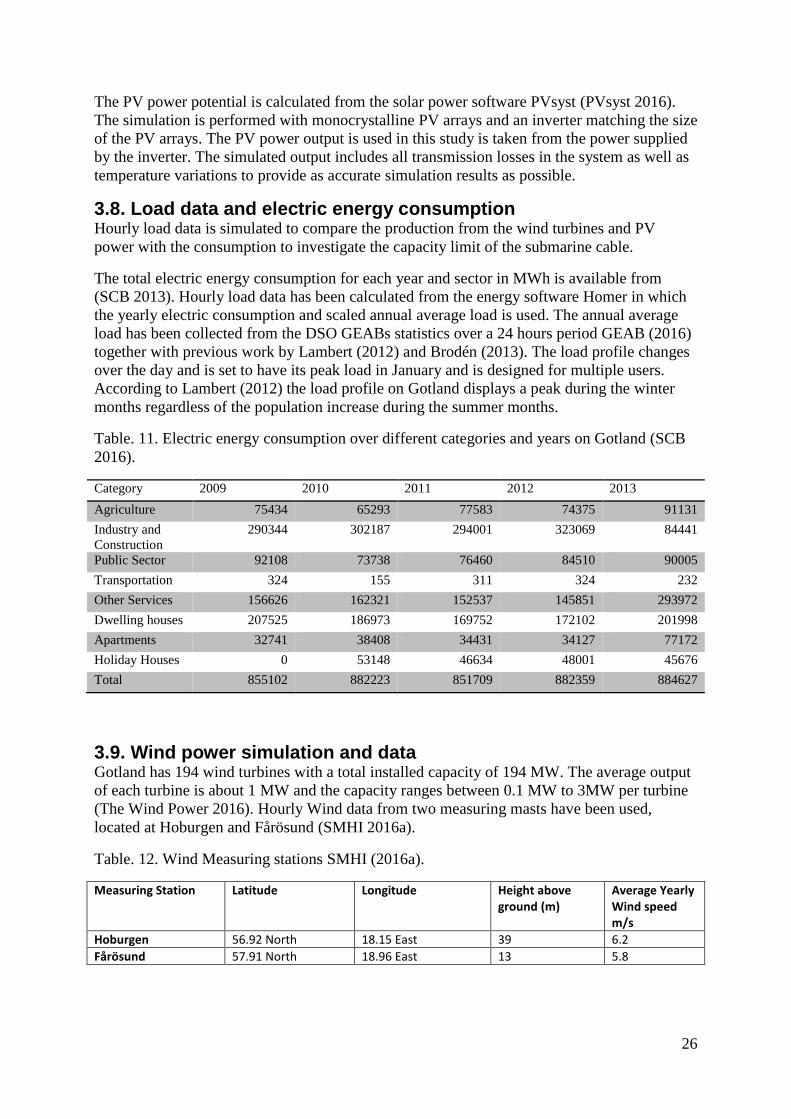
Table. 11. Electric energy consumption over different categories and years on Gotland (SCB
2016). ........................................................................................................................................ 26
Table. 12. Wind Measuring stations SMHI (2016a). ............................................................... 26
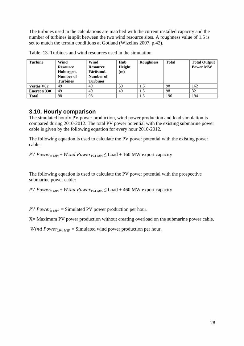
Table. 13. Turbines and wind resources used in the simulation. ............................................. 28
Table. 14. Total PV power potential on Gotland 2010-2012. The total PV power potential is
calculated to be 667 MW. ........................................................................................................ 29
Table. 15. Summary of each building types potential 2010-2012............................................ 30
Table. 16. Type Buildings share of total output. ...................................................................... 30
Table. 17. Maximum and Minimum PV power production 2010-2012. .................................. 30
Table. 18. Simulation of 194 MW Wind Power in Homer Legacy. ........................................ 31
Table. 19. Maximum and minimum wind power production 2010-2012. ............................... 31
Table. 20. Load profile Gotland. .............................................................................................. 32
Table. 21. Hours of overload 2010-2012 with the current submarine power cable. With the
existing wind power of 194 MW and 0 to 667 MW of PV power. .......................................... 35
Table. 22. Maximum PV potential with the existing power cable with a capacity of 160 MW
and 194 MW wind power 2010-2012. ..................................................................................... 35
Table. 23. Hours of overload in 2010-2012 with the addition of the prospective power cable.
With existing wind power of 194 MW and 500-667 MW of PV power. ................................. 36
Table. 24. Maximum PV power potential with the addition of the prospective submarine
power cable with a total capacity of 460 MW and 194 MW wind power 2012-2012. ............ 36

VIII
List of Figures
Fig. 1. Generated electricity in Sweden by energy source during 2013 (SEA 2014). ............... 3
Fig. 2. Solar Radiation in Sweden .Used with permission from SMHI (SMHI 2014). ............ 5
Fig. 3. Flow Chart of the method of determining the PV power for building (Weiss & Widén
2012). ........................................................................................................................................ 16
Fig. 4. Most common building type according to (Kjellsson 2000). Dwelling building with 1.5
floors and a Saddleback roof with a tilt of 30 degrees. ............................................................ 18
Fig. 5. Standard dwelling building in relation to the cardinal direction. .................................. 19
Fig. 6. Solar radiation hitting flat respectively tilted surface at 0°........................................... 20
Fig. 7. Solar radiation hitting flat respectively tilted surface at 90°. ........................................ 20
Fig. 8. Solar radiation hitting flat respectively tilted surface at -90°. ...................................... 21
Fig. 9. Solar radiation hitting flat respectively tilted surface at 180°. ...................................... 21
Fig. 10. Distribution of saddleback roofs by azimuth orientation (Weiss & Widén 2012). .... 22
Fig. 11. Optimal installation for PV arrays on a flat roof surface in Sweden. X represents the
height of the PV array Van Noord & Paradis (2011). ............................................................. 23
Fig. 12. Power Curve, Vestas V82 1650 KW. ......................................................................... 27
Fig. 13. Power Curve, Enercon 330 330 KW. .......................................................................... 27
Fig. 14. Total PV power production per month 2010-2012. .................................................... 29
Fig. 15. Monthly values over simulated wind power production 2010-2012. ......................... 31
Fig. 16. Hourly electric load during an average year. .............................................................. 32
Fig. 17. Total consumption per month for average year. ......................................................... 33
Fig. 18. Total RETs production and consumption 2010. ......................................................... 33
Fig. 19. Total RETs production and consumption 2011. ......................................................... 34
Fig. 20. Total RETs production and consumption 2012. ......................................................... 34

IX
Nomenclature
𝐴𝑅𝑜𝑜𝑓= Total roof area (m²)
𝐴𝐹𝑙𝑎𝑡 𝑟𝑜𝑜𝑓 𝑎𝑟𝑒𝑎= Area measured from above (m²)
𝛽= Angle of roof inclination (°)
𝑃𝑘𝑖𝑛 = Power (W)
𝜑= Density (Kg/m³)
V= Wind Speed (m/s)
A= Area (m²)
𝑃𝑉 𝑃𝑜𝑤𝑒𝑟𝑥 𝑀𝑊 = Simulated PV power production per hour
X= maximum PV power production without causing overload on the export cable
𝑊𝑖𝑛𝑑 𝑃𝑜𝑤𝑒𝑟194 𝑀𝑊 = Simulated wind power production per hour
W/m² = Unit of measured global solar radiation used by SMHI
X
List of Acronyms and Abbreviations
AC Alternating Current
CHP Combined Heating and Power
DC Direct Current
DSO Distribution Systems Operator
GEAB Gotlands Energi Aktiebolag
GWH GigaWatt Hour = 1000 MWh
HVDC High Voltage Direct Current
IEA International Energy Agency
IVA The Royal Engineering Academy of Sweden
KV Kilo Volt = 1000 V
kWh Kilo Watt Hour = 1000 Wh
MWh Mega Watt Hour-1000 kWh
PV Photovoltaic
RETs Renewable Energy Technologies
SCB Statistics Sweden
SEA The Swedish Energy Agency
SEPA Swedish Environmental Protection Agency
SMHI Swedish Meteorological and Hydrological Institute
STA Swedish Tax Agency
STC Standard Test Conditions
TSO Transmission Grid Operator
TWh Terra Watt Hour = 1000 GWh
VRE Variable Renewable Energy


1
1. Introduction A sustainable future requires a transition towards a fossil free energy usage and a renewable
electric production. Future electric energy solutions have to accommodate increased demand,
energy efficiency and renewable production (Sheffield 1998). With an annual growth rate of
2.6% the worldwide energy demand is predicted to increase by 60% in 2050 compared to
2010 (Reilly et al. 2015, p.4). Sweden has the third largest electricity consumptions per
capita among the International Energy Agency (IEA) members (IEA 2013, p.107). The
energy demand in Sweden is predicted to increase in the future due to increased immigration
as well as economical and industrial growth (IEA 2013, p.23). There is also a predicted
increase of electricity as an energy carrier during a transition towards heat-pumps instead of
oil, electric motors instead of gasoline engines and diesel engines (Sköldberg et al. 2010,
p.15). At the same the remaining ten nuclear reactors built in the 1970s which are providing
between 40-50% of the Swedish yearly electricity demand are getting old and there are no
current plans to replace them (IEA 2013, p. 95).
Renewable primary energy sources such as wind, hydro, biomass and photovoltaics account
for about 60% of the yearly generated electricity in Sweden (IEA 2013, p78pp). 80% of the
renewable energy production comes from hydro power, making it the largest contributor when
Sweden reached the 2020 targets of 50% renewables in 2013 (IEA 2013, p.85). Sweden has
fully developed its hydro power potential and the remaining large rivers are preserved due to
environmental concerns1. Therefore, other types of renewables have to be utilized to meet the
future demands if carbon-emissions are to be kept on similar levels (IEA 2013, p.129). One
particular region that has a large share of renewables is the island Gotland. The local power
company and distribution systems operator (DSO) GEAB has worked together with the
municipality, private and government-owned companies to promote wind turbines (Region
Gotland 2006). Gotland was the first test site for large turbines in the late 1970s and has
currently 194 wind turbines operational (Wizelius 2007, p.44); The Wind Power 2016).
Apart from favourable wind conditions, Gotland has the most sunshine hours in Sweden and
excellent conditions for Photovoltaic (PV) power systems (SMHI 2016). PV power is
becoming more popular with both residential and commercial use (Lindahl 2014). Decreased
costs and governmental support are two contributing factors as the installed capacity has
doubled every year since 2010 (Lindahl 2014, p.3). Just as wind power development requires
wind resource maps to estimate the potential production, PV power can be assessed in a
similar way. Multiple regional studies have been carried out to determine the PV power
potential on existing buildings. For example Lingfors & Widén (2014), Weiss & Widén
(2012) and Kamp (2013). Gotland is located about 80 km from the mainland of Sweden and
recieves its electric power supply by two submarine power cables (GEAB 2016). The capacity
of the power cables determines how much electric energy Gotland is able to export and
consume at any given time (Axelsson et al. 1999). A prospective submarine power cable with
increased capacity is planned to be installed in 2021 to enable further renewable energy
technologies (RETs) development (SEA 2016). Gotland provides a unique case of a region
with great wind and solar resources limited by the electricity export capacity by the power
cable.
1 To maintain the landscape as hydropower requires river diversions and dams (IEA 2013, p.129).

2
1.1. Aims and objectives This paper aims to investigating the theoretical solar PV power potential on existing buildings
on the Swedish island Gotland by including existing wind power production, electric load and
the power cable during 2010-2012.
1.1.1. Research Questions What is the theoretical PV power potential for existing buildings on Gotland?
How is the theoretical potential spread between industrial buildings, dwelling buildings,
multi-dwelling buildings and other buildings?
How will a combination of a large share of PV power and wind power perform on Gotland
with the restrictions of the current and prospective submarine power cables?
How much PV power can be installed on Gotland considering the current and prospective
submarine power cables?

3
1.2. Background The energy mix in Sweden relies heavily on hydro- and nuclear power. Any future scenario
without nuclear power requires an increased share of renewables (IEA 2013, p.24).
Fig. 1. Generated electricity in Sweden by energy source during 2013 (SEA 2014).
The Swedish island of Gotland has a large proportion of RETs in the energy mix. 194 wind
turbines with a combined output of 194 MW provide about 40% or 417 GWh per year of the
total electricity demand (Region Gotland, 2015; SCB, 2013). The regional municipality has a
vision of a climate neutral electricity production in 2025 as well as being cutting edge when it
comes to island based climate and energy solutions (Region Gotland 2010). As part of this
vision, the county administrative board runs a yearly energy seminar to discuss and assess
current and potential RETs opportunities (Region Gotland 2011). Current campaigns in the
latest energy plan from 2010 focused on local renewable resources such as wind power,
biogas, biomass and solar power. In the future, an increase to a total of 500 turbines with a
rated output of 1500 MW is regarded to be possible (Region Gotland 2006). The Energy plan
states that an installed capacity of about 20 MW PV power in 2025 is possible, which would
only provide a small share to the total electricity demand, about 2% of the total end use
(Region Gotland 2006). There is no official regional statistics for installed capacity for PV
power in Sweden but as seen in (fig. 1), the yearly production was only 35 GWh in 2013.
According to Lindahl (2014) the cumulative installed PV power capacity was 79.4 MW in
2014.
When it comes to solar radiation, Gotland has the best conditions for PV power in Sweden as
seen in (fig. 2), with an annual irradiance of about 1050 kWh/m² per year. Regardless of the
good conditions for PV power, wind power has been the dominating RETs on Gotland since
the first experimental wind turbines were developed in the late 1970s (Wizelius 2007, p.18).
Increased local electricity generation will require reinforced infrastructure and an additional
submarine power cable to export surplus electric production (Region Gotland 2011). The
41% 43%
10% 6%
0%
Hydro Power 60935 GWh
Nuclear Power 63597 GWh
Combined Power and Heating 14789
GWh
Wind Power 9842 GWh
Photovoltaics 35 GWh

4
existing power cable consists of two high-voltage direct current (HVDC) links with a capacity
of 160 MW each (GEAB 2016). One of the power cables is designated for one way
transmission to Gotland and the other is bidirectional so a total of 160 MW can be exported at
any given time (Axelsson et al. 1999). A prospective submarine power cable is planned to be
installed in 2021. The current limit, due to electricity export limitation for RETs on Gotland is
195 MW and the prospective power cable will increase the limit to 500 MW (Gotlands
Kommun 2010; SVK 2016).

5
Solar Radiation in Sweden
Fig. 2. Solar Radiation in Sweden .Used with permission from SMHI (SMHI 2014).
6
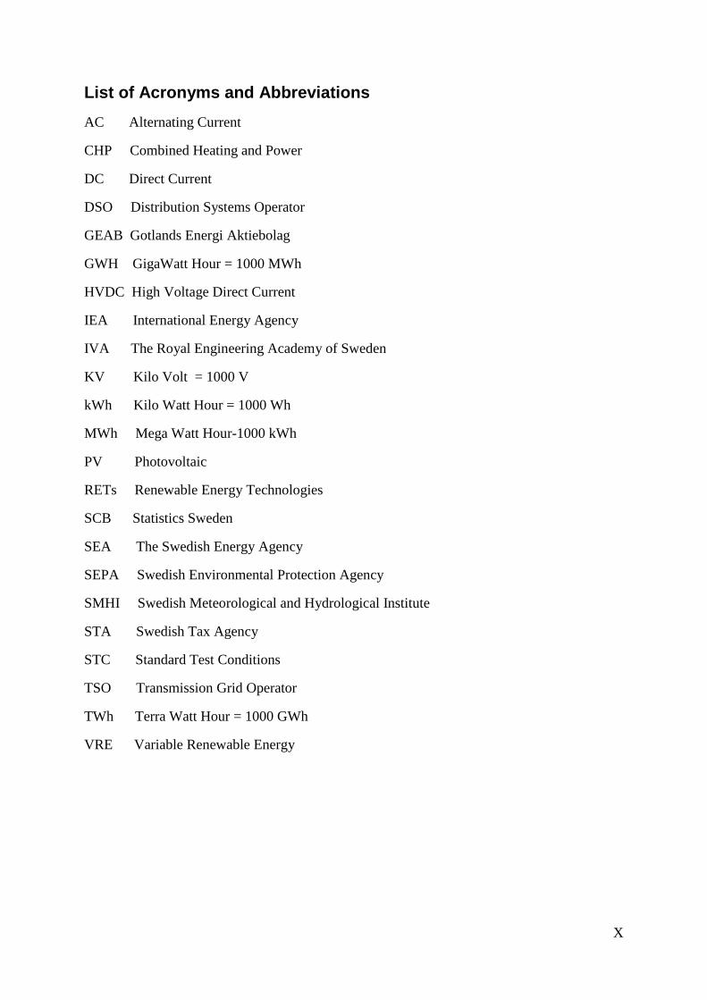
1.2.1. Environmental goals and Future scenarios The future for the Swedish electricity sector needs to be decided in the coming years due to
aging nuclear power stations and the estimated increase in electricity demand. Sweden’s
national environmental policy is divided into 16 environmental quality objects. The objectives
are to be met within one generation (2050) and the actions required to achieve these goals are
stated in the generation goal policy (SEPA 2016). To meet these 16 objectives until 2050, a
transition towards a sustainable thinking in every sector and part of society is required. This
means that the energy sector has to change and different future scenarios are currently being
investigated. Four of these goals are directly linked to electricity generation:
Reduced Climate Impact.
Clean Air.
Natural Acidification Only.
A Good Built Environment.
SEPA (2016)
The Royal Engineering Academy of Sweden (IVA) has investigated the different pathways
Sweden can take to meet the environmental goals and the electricity demand (Byman &
Nordling 2016). The available electrical generation options, hydro, nuclear, biofuel, wind
power and PV power are reviewed with regard to their maximum potential. IVA estimations
are based on a future scenario with a peak demand of 26-30 GW and an annual demand of
140 – 200 TWh2.
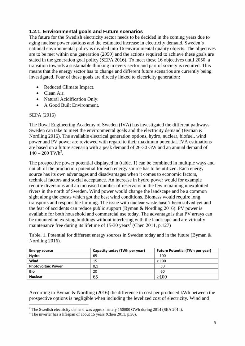
The prospective power potential displayed in (table. 1) can be combined in multiple ways and
not all of the production potential for each energy source has to be utilized. Each energy
source has its own advantages and disadvantages when it comes to economic factors,
technical factors and social acceptance. An increase in hydro power would for example
require diversions and an increased number of reservoirs in the few remaining unexploited
rivers in the north of Sweden. Wind power would change the landscape and be a common
sight along the coasts which got the best wind conditions. Biomass would require long
transports and responsible farming. The issue with nuclear waste hasn’t been solved yet and
the fear of accidents can reduce public support (Byman & Nordling 2016). PV power is
available for both household and commercial use today. The advantage is that PV arrays can
be mounted on existing buildings without interfering with the landscape and are virtually
maintenance free during its lifetime of 15-30 years3 (Chen 2011, p.127)
Table. 1. Potential for different energy sources in Sweden today and in the future (Byman &
Nordling 2016).
Energy source Capacity today (TWh per year) Future Potential (TWh per year)
Hydro 65 100
Wind 15 ≥ 100
Photovoltaic Power 0,1 50
Bio 20 60
Nuclear 65 ≥100
According to Byman & Nordling (2016) the difference in cost per produced kWh between the
prospective options is negligible when including the levelized cost of electricity. Wind and
2 The Swedish electricity demand was approximately 150000 GWh during 2014 (SEA 2014).
3 The inverter has a lifespan of about 15 years (Chen 2011, p.36).

7
PV power is regarded as variable renewable energy (VRE) as the electricity production
changes with the weather and the seasons. The IVA report does not state that all of the peak
demand need to be met by Swedish production but it requires the annual demand to be met
(Byman & Nordling 2016). This is because the national grid has 16 international connections
so Sweden can export and import electricity when needed to meet short term deficits (Byman
& Nordling 2016).
1.3. Sustainable development and research mode The first adopted definition of sustainable development derives from the Bruntland report
which stats: "Development that meets the needs of the present without compromising the
ability of future generations to meet their own needs." (Brundtland et al. 1987). Robèrt et al.
(2010) has expanded the original definition and formulated four principles that can be used as
guidelines when taking actions towards a sustainable society:
In a sustainable society, nature is not subject to systematically increasing …
1. concentrations of substances from the earth’s crust.
2. concentrations of substances produces by society.
3. degradation by physical means.
(Robèrt et al. 2010, p.99)
These guidelines can be used when assessing the actions we take towards sustainability as
they emphasize the earth to be viewed as a closed system (Robèrt et al. 2010, p.99). An
important part of sustainable thinking is to improve and rethink current technologies as well
as investigating future scenarios (Robert et al 2004, p.20). When sustainability is referred to in
an energy context it is often synonymous with renewable energy. This is correct when
renewable energy sources comply with the sustainability definitions. Compliance with all
three sustainability principles requires not only a sustainable energy production but also a
sustainable system approach, including construction, maintenance and local impact
(Ramachandra & Shruthi 2007). Hydro power and wind power can for example degrade the
nature by altering the landscape and interfere with the wild life (Wizelius 2007, p.194).
Sustainable electricity production is one part in the challenge to a sustainable future and
should be seen as a part in a larger system approach (Ramachandra & Shruthi 2007).
Sustainable electricity production requires pilot studies of the different renewable options to
assess the potential power output for specific regions and the environmental impact
(Ramachandra & Shruthi 2007).
One research field is to calculate the potential for PV systems on existing buildings. The
problem is that not all buildings are suitable for PV systems with regard to shading, tilt and
azimuth angle (Chen 2011, p.83). The energy content of the solar radiation is also regional
specific, making general estimations uncertain. Regional PV power potential studies has been
carried out in Sweden by Lingfors & Widén (2014), Weiss & Widén (2012), Ekström (2012)
and (Kamp 2013). All of these are based on methods by Weiss & Widén (2012) and Kjellsson
(2000)4 using global irradience data from the SMHI model STRÅNG (SMHI 2016. Weiss &
Widén (2012) found the largest PV power potential to be on dwelling buildings, 443 GWh per
year in Dalarna. A total potential of 670 GWh per year included dwelling buildings, multi-
dwelling buildings, supplementary building and industrial buildings if the available roof area
of 6956000 m² were used (Weiss & Widén 2012). In Blekinge, the total PV potential was
4 Further explained in Section 3.

8
calculated to be 1200 GWh per year with an available roof area of 17000000 m² and 440
GWh for dwelling buildings (Lingfors & Widén 2014). More detailed studies using light
detection and ranging (Lidar) data have been performed by Jakubiec & Reinhart (2013) and
Brito et al. (2012) to determine the PV power potential in Cambridge and Lisbon. When
studying the regional PV power potential it is also of interest to know when the electricity
production will occur. An increased share of renewables in the energy mix will make these
kind of predictions extra important as electricity output from renewables fluctuate more
compared to thermal power stations (Rowlands et al. 2011). The electricity price is also
dependent on the supply and demand of electricity and knowing when PV systems will
generate electricity helps with the investment calculation (Rowlands et al. 2011).
The combination of wind power and PV power has been studies by Buttler et al. (2016). They
compared PV power and wind power production with load data on a national and regional
level in the EU member states. By using time series data from the transmission grid operators
(TSO) their results displayed a variation in wind power production with peak production
during the winter and PV power production peaks during the summer. Less variation were
found in wind power compared to PV power (Buttler et al. 2016). In all EU membership
countries the maximum PV power production was 66% of the installed capacity and for wind
power 61%. On a national level the wind power production reached 100% of the installed
capacity and PV power between 70-90% of the installed capacity (Buttler et al. 2016).
1.3.1. Previous Photovoltaic power potential studies on Gotland One previous study of PV power potential has been performed on Gotland by (Ekström 2012).
Ekström (2012) calculates the PV power potential from the gross space area of the type
building found in the real estate tax assessments by Swedish statistics (SCB) and estimations
on building size for non-residential buildings by Weiss & Widén (2012). The number of
buildings derives from the building statistics supplied by Swedish statistics and the DSO
GEAB for non-residential and industrial buildings. The study includes a net debit model in
which the generated electricity on a monthly or yearly basis can be deducted from the
electricity bill. The PV power potential was calculated to be 117 GWh per year for dwelling
buildings and a total of 242 GWh per year for all investigated building types during 2010
(Ekström 2012). If heritage buildings were to be excluded the PV power potential was instead
231 GWh per year. The potential PV power capacity is not declared. The net debit model did
not change the PV power potential if used on a yearly basis but reduced the potential if used
on a monthly basis for dwelling and multi-dwelling buildings (Ekström 2012). The study
focuses on the correct sizing of PV power for each type building during different economical
compensation schemes.

9
1.4. Delimitations The investigated building categories are those that are available from Statistics Sweden. It
excludes military buildings, power stations, and other special government and private
buildings such as communication buildings and waste-water treatment plants (SCB 2016a).
The building data is only available for 2010, compared to the solar radiation data which is
available on a yearly basis since 1999 (SMHI 2016). However, the building stock decreases
and increases slowly over time. On a national level about 1% per year (SCB 2010), therefore
it should not impact the accuracy of the PV power potential estimations significantly. Other
methods to determine the PV power potential derives from studying Lidar maps which
provides more accurate results as the roof area is being directly mapped from above. The
Swedish mapping, cadastral and land registration authority (Lantmäteriet) are currently
working on a Lidar map for Sweden and the project is estimated to be finished in 2017
(Lantmäteriet 2016). Lidar maps for certain areas are available as of today and there is also
studies using Lidar data derived from private and municipal initiatives, for example (Jonsson
& Lindberg 2011). As there is no high resolution Lidar data available for Gotland and the
detailed vector property map is not available for students, this paper follows similar methods
to the work by Kjellsson (2000) and Weiss & Widén (2012). Possible limitations of the local
distribution and regional grid are also not included in this paper, only the limitation for the
current and prospective submarine power cables. The PV power production, wind power
production and load data are all derived from simulations over a three year period. Therefore
the results should be used carefully. Wind speeds in particular can vary significantly over time
and when comparing simulated production with real production a wind index can be used.
The average wind speed at a site is measured over several years and the amount it deviates
from a single year’s measurements is referred to as the wind index (Wizelius 2007, p.52).
This study uses hourly values to determine the electricity production and overload. Electricity
is however consumed and produced instantly; leaving a bias that it can display peaks and dips
within the hour. This could potentially lead to overestimations of the PV power potential.
1.4.1. Solar PV Potential method There are many methods and definitions when determining the PV power potential. This
study examines the PV power potential for existing buildings by determining the roof area
from the ground space area. Each building category is assigned a roof tilt and a set of limiting
factors, azimuth angle, shading, and obstacles. The political and economic potential is not
investigated. This is a widely used method but with the development of Lidar data more
accurate results can be achieved.
10
2. Theory This chapter describes the theory behind PV systems, wind power and the electric grid.
2.1. Solar Radiation Direct radiation is the radiation that hits the ground unimpacted by the athomsphere. During a
cloudy day the direct radiation measured on the ground will be zero as the direct radiation has
been scattered by the clouds. Instead it is measured as diffuse radiation. Smog and water
vapour can also scatter the direct radiation, even on a sunny day, the surface of the earth will
experience a combination of direct and diffuse radiation. Albedo, or the reflection coefficiant
of surrounding surfaces discribes how much radiation that is being refleced from an object or
a surface (Ineichen et al. 1990). In Sweden the mean value is 20% but it depends on the
properties of the surface, snow for example has an albedo between 50-80% (Weiss & Widén
2012). The reflected radiation deriving from both direct and diffuse radiation is called ground-
reflected radiation.
Direct, diffuse and ground reflected radiation together determines the production of the PV
cell and it is refered to as global radiation, measured in W/m² by SMHI. The average global
radiation in Sweden is about 1 kWh/m² per year (Persson 2000).
2.1.1. Tilt, Angle, Latitude The amount of global radiation hitting a flat surface depends on the latitude and the time of
the day. The amount of direct radiation hitting a tilted plane is also dependent of the azimuth
angle and the tilt of the plane.
2.2. Photovoltaic Cells About 90% of the PV cells produced and used today are constructed out of crystalline silicon
(Saga 2010). How they utilize the photoelectric effect to produce electricity as described
below
Photovoltaic cells are constructed out of two or more semiconducting layers, usually made out
of silicon. The different semiconducting layers are referred to as the p-layer and the n-layer.
The p-layer is constructed of boron doped silicone, giving it a positive potential (Saga 2010).
The n-layer is constructed so that it has an abundance of electrons from being doped in
phosphorous, giving it a negative potential. The n-layer is on top of the p-layer, creating a
band gap between the two layers. The band gap represents the minimum energy required to
excite an electron from its bound state into its free stage. The energy of the incoming photons
determines if they will interact with the layers, if the photon has less energy than what is
required by the band gap it will not excite the electron (Saga 2010). If the photons energy is
equal or above the band gap it will be absorbed and excite the electron. When a photon with
enough energy hits the n-layer it excites a negative charged electron, which migrates to the p-
layer creating a potential difference. If the PV cell is connected to a load the electrons will
flow through the load and create work (Chen 2011, p.150ff).
The voltage of the PV cell is determined by the band gap between its layers. The larger the
band gap is, the higher is the voltage but a high band gap also requires high energy photons.
The band gap is therefore matched with the energy content of the centre of the solar spectrum.
A solar module consists of many PV cells which are serially connected to increase the voltage
output (Chen 2011, p.130).

11
2.2.1. Inverter PV cells produce direct-current (DC) and the power grid is designed for alternating current
(AC). PV cells in a grid-connected PV system are connected to an inverter. The inverter
changes direct current into alternating current to the desired voltage and frequency. Swedish
standard is 230 V and 50 Hz (Moren 2013). Depending on the system design, multiple PV
arrays can either be connected serial or parallel. Serial connection increases the voltage and
parallel connections increase the current. There are also combinations of the two installation
methods and the installation method depends on the inverter specifications (Chen 2011,
p.176ff).
2.3. Types of Photovoltaic Cells Crystalline PV cells can be divided in two main categories, monocrystalline and
polycrystalline. Thin film PV cells can be made out of a number of materials in which silicone
is one (Chen 2011, p.90). In order to compare the efficiency of different PV cells Standard
Test Conditions (STC) following the IEC 60904-1 are used which states the following
conditions (Muñoz-García et al. 2012).
Irradiance: 1000 W/m².
Cell temperature: 25°.
Spectral distribution: AM 1.5 (according to IEC 60904-3) (Geneva, 2008).
(Muñoz-García et al. 2012)
2.3.1. Polycrystalline Polycrystalline cells are made out of casted silicon which produces a mixture of crystal
shapes. This makes them less efficient compared to polycrystalline cells but they are also less
expensive and the production process produces less waste. They have an efficiency (STC) of
13-16% (Energy Informative 2016).
2.3.2. Monocrystalline Monocrystalline cells are made out of very clear crystal in which the molecules are perfectly
aligned with each other. This gives monocrystalline cells a better performance and the
efficiency is usually between 15- 20% (STC). The production process is more demanding and
only the best silicone can be used which increases waste in the production process (Energy
Informative 2016).
2.3.3. Thin-Film Thin-film PV cells have increased its market share lately to about 5 % of the installed
capacity worldwide in 2015 (Energy Informative 2016). They can be made out of a number of
photovoltaic elements. Some of the photovoltaic elements used are very efficient at capturing
the solar radiation which is why they can be made very thin and they are generally considered
to have an advantage over silicon cells to capture diffuse radiation (Energy Informative 2016).
For commercial use the efficiency is between 10-16% but there are research projects that have
developed thin-film cells with 20% efficiency which is 2/3 of the theoretical efficiency of PV
cells (UU 2016).
2.4. Wind speed and the power of the wind The wind speed at a specific site and altitude depends on a multiple of meteorological and
terrain factors. Rough terrain and obstacles decreases the wind speed and creates turbulence
and hills can increase the wind speed up to certain altitudes. The terrain can be divided into
multiple roughness classes in which open sea is given roughness class 0 and large cities 4
(Wizelius 2007, p.42). This classification is used when creating wind resource maps for

12
suitable areas and in wind energy software to simulate the electrical production. The power of
the wind is proportional to the cube of the wind speed and depends on the density of the air
(Wizelius 2007, p.44ff).
The following equation is used for calculating the power of the wind:
𝑃𝑘𝑖𝑛 =1
2 𝜑𝐴𝑉3
𝑃𝑘𝑖𝑛 = Power (W)
𝜑= Density (Kg/m³)
V= Wind Speed (m/s)
A= Area (m²)
(Wizelius 2007, p.48)
Wind turbines are designed to work at certain wind conditions with a cut-in speed between 3-
4 m/s and a cut-out speed of about 25 m/s. The rated output power of the turbine is reached at
a certain wind speed which remains constant until the cut-off speed in which the turbine
moves away from the wind to stop damage. This is referred to as the wind turbines power
curve (Wizelius 2007, p.120ff). As the wind speed increases, a 2 MW turbine will produce
less before it reaches its rated output power of 2 MW at 15 m/s and will continuously produce
2 MW while the power control reduces the speed of the turbine to avoid damage (The Danish
Wind Industry Association 2003).
2.5. Electrical grid The electrical grid in Sweden has originally been constructed to accommodate electric power
production from hydroelectric power in the north with electric power consumption in the
more populated southern parts.
2.5.1. National grid The National grid is owned and operated by Svenska Kraftsnät (SVK) a state-owned electric
transmission systems operator. SVK has the overall responsibility of the grid including
balance management in which they have the authority to order power companies to increase
or decrease production as well as cut of electricity to energy intensive industries in case of
severe drop-outs. The voltage in the transmission grid is between 220 and 400 kV (SVK
2015).
2.5.2. Regional grid The regional grid is owned by a number of private companies and is connected to the national
grid to provide electricity to sub-regions. Certain industries can be connected to the regional
grid as well as medium sized power stations or wind turbines. The voltage of the regional grid
does not exceed 220 kV (SVK) 2015).
2.5.3. Distribution grid The distribution grid provides electricity to the household consumer, industry and utilities.
The end user is usually connected to a 400 V three-phase system (SVK 2015).

13
2.5.4. Price areas The Swedish electrical grid is interconnected to its neighbouring countries and the price of
electricity for the northern and Baltic countries are set on the power exchange market Nord
Pool. To comply with EU market regulations Sweden has since 2008 been divided into four
bidding areas to enable fair market conditions between all bidding areas on Nord Pool (SVK
2015). Price areas are constructed so that areas with a lot of electric generation will have a
lower price (Nordpool 2016).
2.6. Distributed generation Electricity has traditionally been produced in large centralized power stations and transmitted
in the national grid to high consumption areas. Hydro-electric production in the rivers in the
north of Sweden, wind power parks in coastal regions such as Gotland with good wind
resources as well as off-shore wind parks can be connected to the national or regional grid if
they are large enough (Wizelius 2007, p.206). However with distributed RETs, production is
becoming decentralized and production is shifted towards areas with favourable conditions
such as a few wind turbines on farm land, PV systems on buildings and existing but very
limited, residential wind turbines (SVK 2015). As the distribution- and regional grid is built
for one way transmission from the power station to the consumer, distributed generation
provides challenges for the DSO as the grid now have to accommodate bidirectional power
distribution. However depending on the existing infrastructure, a certain amount of additional
power production is usually possible. The upper limit of additional power production that can
be connected to the grid is called hosting capacity (Kupzog et al. 2014). The hosting capacity
has been described by Yang & Bollen (2008) as:
”The hosting capacity is defined as the maximum distributed generation (DG) penetration for
which the distribution network still operates according to design criteria and network
planning practices based on the European standard EN50160” (Yang & Bollen 2008).
The main issue with distribution generation in the local distribution grid is voltage rise and
overload on the power cables and transformers. The power quality in the grid is regulated by
the Electricity Act and states that the acceptable variations for a number of parameters (Moren
2013). The Swedish end consumer in the low voltage distribution grid is connected to a 400 V
three-phase system with a frequency of 50 Hz. The acceptable voltage variation is ±10% and
the unbalance between the three phases can’t exceed 2 % during any ten minute interval
measured over a week (Moren 2013). PV systems connected to a single phase inverter can
contribute to unbalanced circuits and therefore the recommendation is to install a maximum of
3 KW PV power to a single phase inverter (Chen 2008: 210). When production is high and
the consumption is low, usually during noon in the summer, PV systems can increase the
voltage in the distribution grid. The maximum hosting capacity of the distribution grid can
therefore be estimated by the worst case scenario of which there is no consumption and
maximum production (Yang & Bollen 2008). Studies of the hosting capacity in the Swedish
low voltage distribution grid, for example Walla (2012, p.44) found larger hosting capacity in
the city grids compared to those on the countryside.
2.7. Electrical grid on Gotland The electrical grid on Gotland is connected to the Swedish mainland by two HVDC
submarine cables. The current cables are designed so that one cable is bidirectional with the
ability to export surplus electricity while the other remains one-way transmissions to Gotland
to ensure electricity demand and grid stability as well as frequency reference (Axelsson et al.
1999). To supply Gotland with electricity during Island mode, two gas turbines of 60 MW
each are located in Slite as the main backup power (GEAB 2016). There is also a diesel power

14
station in Visby producing 36 MW, four gas turbines in Bäcks of 12 MW and two 10 MW gas
turbines operated by the industry Cementa (Lambert 2012). According to SVK and the local
power company GEAB, the maximum capacity of the exporting submarine cable has been
reached by the wind power capacity (SVK 2015; Geab 2016). The current capacity limit of
RETs at Gotland is set at 195 MW installed capacity (Brodén 2013). This is more than the
submarine cable can export but is considered to be the upper limit by the DSO (GEAB 2014).
To enable further wind power development and Gotland’s long term energy stability, a
prospective submarine power cable with a capacity of 300 MW will be installed in 2021. The
prospective cable will operate together with the old cables increasing the RETs capacity to a
total of 500 MW (SVK 2015).
2.8. Microgeneration The majority of PV systems are connected to the low voltage distribution grid. No official
statistics for the share of PV systems connected to the low voltage distribution grid are
available in Sweden, but for Germany the share is over 85% in Germany (Kupzog et al.
2014). In Sweden, everyone with an electric meter has the right to install a RETs system and
connect it to the meter. The power company is obligated by law to change the electric meter
and reinforce the grid if necessary (SEMI 2015). As the electricity market is deregulated there
is no obligation for a power company to purchase the surplus electricity from the micro
producer but there are many companies to choose from that will buy the surplus electricity
and it doesn’t have to be the same company as the grid operator (SEA 2016). Current
regulations require the following two demands to be met to qualify as a micro producer:
Maximum installed power production capacity of 43,5 KW.
Larger electricity consumption than electricity production from RETs on a yearly
basis.
(SEA 2016)
As of 2015 there is both a tax support system and an investment cost support system available
for micro producers. The tax reduction is SEK 0.60 for every surplus kWh produced and is set
to maximum SEK 18000 per year (STA 2016). The investment support system is frame-
limited with a governmental contribution of SEK 225 million in 2016 and SEK 335 million
each year from 2017-2019. The maximum support for each facility is SEK 1,2 million or 20%
for private individuals and 30% for companies (SEA 2016).
2.9. Electric load The electrical grid needs to be in balanced at all times with an electrical supply meeting the
electrical demand. To guarantee power supply, production is split between base load power
plants which provide stable and cheap electricity together with load following power plants.
These should be easily adaptable to alter the output and gas-turbines and hydroelectric power
plants provide this roll (Camacho et al. 2011). Wind power and PV power production depends
on the weather and therefore require a larger share of load following power plants to step in
and guarantee production (Chen 2011, p.46). The demand side or load changes with the
seasons; more electricity is used for heating during the winter in northern countries compared
to more electricity used for air conditioning in southern countries. In a domestic situation the
consumption changes during the day with peaks during the morning and evening when people
are home from work. Industries can have a steady load if they are operated day and night
(Chen 2011, p.51).

15
The situation on Gotland with a large share of wind power and a limited population means
that when the wind turbines output is maximized the production is greater than the load and
electricity needs to be exported by the submarine cable to other users. A scenario with
production from both PV power and wind power, requires that the output to be determined
together with the load to see if the limit of the submarine cable is meet during any given time.
The load profile on Gotland displays peak demand during the winter months regardless of the
population increase during the summer (Lambert 2012).

16
3. Methods and Data The method section describes the process of determining the available roof area for PV cells
when being calculated from the ground space area and wind power production. This process
can be seen in (Fig. 3).
Fig. 3. Flow Chart of the method of determining the PV power for building (Weiss & Widén
2012).
3.1. Solar radiation Solar radiation data has been collected by SMHI since 1961, and after 1983 due to increased
climate concern the radiation measuring program increased in size and has of today 12
measuring stations in Sweden (Persson 2000). SMHI measures solar radiation on a horizontal
surface at an altitude between 4-15 meters with a pyranometer, a type of radiometer used to
measure solar radiation (Persson 2000). The uncertainty of the hourly measurements is
estimated to be between 3-4% and 2% for the yearly values. The solar radiation database
STRÅNG has hourly values over radiation in Sweden since 1999 and global irradience can be
aquired directly in the database (SMHI 2016). The following measuring station in (table. 2) is
used throughout the study.
Table. 2. Visby Measuring Station (SMHI 2012).
Measuring station Latitude Longitude Average Global
Radiation per
between 1999-
2015 kWh/m²
Visby 57.67 North 18.35 East 1046
3.2. Building types and building area The building data is collected from SCB in which the total building area and ground space
area can be extracted on both national and regional level. A building is according to the
Swedish planning and building act:
“A permanent structure intended for occupation by people consisting of a roof and/or walls
and is permanently placed on the ground or completely or partially below the ground or
permanently placed in water”5 (SFS 2016, p. 252).
The data is being updated every five years and the only available data as of today is from
2010 (SCB 2010). The building categories in the SCB data derives from the real property
register and are matched with the Cadastral map from The Swedish mapping, cadastral and
land registration authority which displays property and land ownerships (SCB 2010). If the
5 Translated by the author
Ground Space Area
Roof Type
Roof tilt Azimuth
Angle
Limiting factors, Shade,
obstacles etc
Available area for
PV arrays

17
two registers don’t match the building is categorized as uncoded. The number of buildings
and ground space area derives from the real property register. Ground space area is the area of
the building including its outer walls (SCB 2010). The buildings are organized in four
categories with the category other buildings including Building for public service purpose,
Building for business purpose, Outbuilding, Supplementary building. The following building
categories are used throughout the study.
Dwelling
Multi-Dwelling Building
Industrial Building
Other Buildings
3.2.1. Roof Shape and angle All buildings in the same category do not have the same roof shape but according to Kjellsson
(2000) there is a pattern for the different building categories. The majority of dwelling
buildings are constructed with a saddleback roof as shown in (Fig. 4). Mansard, flat, one-
sided and other types of roofs exist as well but are not as common. The most common tilt of
the saddleback roof is 30 ° which is used throughout in this study (Kjellsson 2000). Industrial
buildings roof shape have not yet been categorized but in studies such as Weiss & Widén
(2012) and Lingfors & Widén (2014) a flat roof is used.
3.3. Building categories
Table. 3. Building category and characteristics (Kjellsson 2000; Weiss & Widén 2012).
Building Category Roof Pitch° Roof Type%
Dwelling 30 Saddleback Roof
Multi-Dwelling
Building
30 Saddleback Roof 85%
Flat Roof 15%
Industrial Building 0 Flat Roof
Other Buildings 30 60% Saddleback Roof
40% Flat Roof

18
3.3.1. Roof Type
Fig. 4. Most common building type according to (Kjellsson 2000). Dwelling building with 1.5
floors and a Saddleback roof with a tilt of 30 degrees.
3.3.2. Roof area
The following equation is used to determine the roof area:
𝐴𝑅𝑜𝑜𝑓 = 𝐴𝐹𝑙𝑎𝑡 𝑅𝑜𝑜𝑓 𝐴𝑟𝑒𝑎
cos 𝛽
𝐴𝑅𝑜𝑜𝑓= Total roof area (m²).
𝐴𝐹𝑙𝑎𝑡 𝑟𝑜𝑜𝑓 𝑎𝑟𝑒𝑎= Area measured from above (m²).
𝛽= Angle of roof inclination (°).
(Weiss & Widén 2012)
3.4. Azimuth angle The azimuth angle describes the compass direction at which an object is located. South equals
0, West 90, East -90 and North 180 (Chen 2011, p.142). A building as seen in (Fig. 5), the
pitched roof sides are facing 90 ° west respectively -90° east. A building with a saddleback
roof will have one side shading the other, how much depending on the azimuth angle and the
hour angle. A flat roof has no shading from the opposite side and the azimuth angle of the
building is insignificant (Chen 2011, p.142). The tilt of the roof is measured in degrees°
relative the horizontal. 0° equals a flat roof and 180° a roof turned upside down (Weiss &
Widén 2012).

19
Fig. 5. Standard dwelling building in relation to the cardinal direction.
The azimuth angle of the building stock is regarded to be undiversified by both Weiss &
Widén (2012) and Kjellsson (2000). However Lingfors & Widén (2014) found that both
dwelling and apartment buildings in the Swedish region of Blekinge displayed a
predominantly angle towards North/South and West/East, as seen in (Fig. 5). Without
available maps, the buildings are estimated to be equable situated on all 360° as seen in (Fig.
11).
3.4.1. Azimuth angles impact on a tilted surface respectively flat surface Figures 6-8 displays the changes in solar radiation hitting a tilted and flat surface depending
on the azimuth angle. The change in production corresponds to changing the position of the
house in (fig. 5), 90° degrees at the time.
Zenith
West
East
South

20
Fig. 6. Solar radiation hitting flat respectively tilted surface at 0°.
Fig. 7. Solar radiation hitting flat respectively tilted surface at 90°.
Jan Feb Mar Apr May June July Aug Sep Oct Nov Dec
Flat Surface (kWh) 0.38 0.98 2.36 4.14 5.8 6.26 5.89 4.54 2.96 1.36 0.47 0.25
Tilted Surface 30° (kWh) 0.85 1.76 3.57 5.2 6.47 6.59 6.35 5.36 4.11 2.34 0.84 0.52
0
1
2
3
4
5
6
7
Ave
rage
kW
h/m
².d
ay
Azimuth Angle 0°
Jan Feb Mar Apr May June July Aug Sep Oct. Nov Dec
Flat Surface (kWh) 0.38 0.98 2.36 4.14 5.8 6.26 5.89 4.54 2.96 1.36 0.47 0.25
Tilted Surface 30° (kWh) 0.41 1.01 2.4 4.13 5.68 6.08 5.78 4.48 2.99 1.42 0.48 0.25
0
1
2
3
4
5
6
7
Ave
rage
kW
h/m
².d
ay
Azimuth Angle 90°

21
Fig. 8. Solar radiation hitting flat respectively tilted surface at -90°.
Fig. 9. Solar radiation hitting flat respectively tilted surface at 180°.
Jan Feb Mar Apr May June July Aug Sep Oct. Nov Dec
Flat Surface (kWh) 0.38 0.98 2.36 4.14 5.8 6.26 5.89 4.54 2.96 1.36 0.47 0.25
Tilted Surface 30° (kWh) 0.41 1.01 2.38 4.1 5.68 6.08 5.75 4.48 2.96 1.41 0.48 0.25
0
1
2
3
4
5
6
7
Ave
rage
kW
h/m
².d
ay
Azimuth Angle -90
Jan Feb Mar Apr May June July Aug Sep Oct. Nov Dec
Flat Surface (kWh) 0.38 0.98 2.36 4.14 5.8 6.26 5.89 4.54 2.96 1.36 0.47 0.25
Tilted Surface 30° (kWh) 0.24 0.5 0.94 2.45 4.27 5.05 4.61 3.05 1.37 0.64 0.31 0.17
0
1
2
3
4
5
6
7
Ave
rage
kW
h/m
².d
ay
Azimuth Angle 180°

22
Buildings with saddleback roofs are distributed to have one side of the roof facing one of the
six lighter areas towards the south, 1/6 in each, see (Fig. 11). The opposite side is facing
north, which is regarded to be unsuitable for PV power due to unfavourable solar radiation
conditions, resulting in very low production (Weiss & Widén 2012).
3.4.2. Buildings azimuth orientation Distribution of building with saddleback roof. 1/6 in each light section with the opposite side
facing north excluded from the calculation.
Fig. 10. Distribution of saddleback roofs by azimuth orientation (Weiss & Widén 2012).
3.4.3. Available area for PV arrays on a flat roofs Flat roofs can seem to be optimal as the azimuth is not of importance as seen in (fig.6) to (fig.
8). But as seen in (fig. 6.), a tilted roof in the optimal azimuth angle receives the most
radiation of all surfaces, almost twice compared to a tilted plane facing north as in (fig. 9).
The optimal tilt depends on the distance from the equator and changes over the year. When
PV arrays are mounted on a flat roof with a tilt, the larger the tilt the more shading occurs
-30
-30
-30
0
30
30
30
180
N
S
W E

23
from the PV array in front which will reduce the PV power production. The optimal tilt for a
flat roof installation is regarded to be 30° when both efficiency and space is taken into
consideration (van Noord & Paradis 2011). PV arrays can’t be mounted to close to each other
because the tilted PV array in front will shade the system behind it. The recommendation to
optimize production on a flat roof is to install the PV arrays with a tilt 30 ° and a distance of
2.5 times the height of the PV-array. By doing so 60% of the flat roof area is available for PV
arrays (van Noord & Paradis 2011).
Fig. 11. Optimal installation for PV arrays on a flat roof surface in Sweden. X represents the
height of the PV array Van Noord & Paradis (2011).
3.5. Additional limiting factors Limitations for PV arrays on roofs include structures such as smoke and ventilation chimneys,
Mansards, drainage, skylights and ladders. Kjellsson (2000) estimates the following
reductions to be suitable for Swedish buildings.
Table. 4. Obstacles on roofs (Kjellsson 2000).
Building Type Reduction%
Dwelling 10%
Multi-Dwelling
20%
Industry 20%
Other 20%
In addition to structural objects of the roof, the surrounding structures such a building and
trees can have a shading effect on the roof, reducing the output of the PV system. This is less
of a problem for standalone buildings on the countryside as seen in (fig. 5.) but can be a
significant limiting factors in cities where most of apartments and public buildings are located
(Kjellsson 2000).
3.5.1. Shading Table. 5. Losses due to shading (Kjellsson 2000).
Building Type Reduction%
Dwelling 10%
Multi Dwelling
15%
Industry 10%
Other 20%

24
3.5.2. Snow and soiling losses Two other factors to consider are snow and dirt on the panels. As PV arrays in Sweden
usually are installed with a tilt of about 30° and the production is low during the winter, snow
is not considered to be a large problem (Kjellsson 2000). Pollen, algae and pollution can soil
the PV array but the reduction from soiling is debatable. However snow and rain will clean
the panels and Mejia & Kleissl (2013) found that PV arrays during a period of 146 days
without rain only suffered a reduction of 7,4% in efficiency. Therefore the effect of snow and
soiling losses will not be included in this study.
3.6. Total reductions Table. 6. Available Roof area after reduction (Kjellsson 2000).
Building Category Reduction Obstacles% Reduction Shading%
Dwelling 10% 10%
Multi-dwelling 20% 15%
Industry 20% 10%
Other 20% 20%
Each of the building categories is given a certain type building that is based on the total
available ground space area divided by the number of buildings. These are then used in the
PV system software, PVsyst to simulate the electric production (PVsyst 2016). The results are
then scaled up by the number of buildings to provide the total PV power potential on Gotland.
3.7. Data and building categorization Table. 7. Buildings, number of buildings and ground space area (SCB 2010).
Building Category Number of buildings
Ground space area of
buildings m ²
Average Size. Area
m ²/Number of
Buildings
2010 2010 2010
Residential building 27591 3722818 135
Industrial building 473 388444 821
Building for public service
purpose 1167 520503 446
Building for business
purpose 752 345390 459
Outbuilding 50 14552 291
Supplementary building 46778 5615888 120
Other building 119 11653 98
Uncoded Missing value 4957 Missing value
Total 76930 10624205 2371
Residential building includes both dwelling buildings, apartment buildings (more than 4
apartments) and small apartment buildings (less than 4 apartments). From the dwelling stock
register, the area and number of dwelling buildings, apartment buildings and other buildings
are used to separate the residential buildings into dwelling buildings and multi-dwelling
buildings and others.

25
Table. 8. Residential buildings divided by category (SCB 2016; SCB (2016a).
Building Category Number of buildings Ground space area of buildings m ² Average
Size. Area
m
²/Number
of
Buildings
2010 2010
Dwelling 17594 2707762 154
Multi Dwelling
Building
9997 1015056 102
From (table.7) the additional buildings are merged into two categories in which Building for
public service purpose, Building for business purpose, Outbuilding, Supplementary building
and other building forms one category and Industry buildings forms another. The categories
are created to make the data handling and result presentation clearer.
Table. 9. Ground space area and number of buildings for all building categories (SCB 2010;
SCB 2016; SCB (a) 2016).
Building category Number Of Buildings Ground space area of buildings m ² Average Size. m ²
2010 2010
Dwelling 17594 2707762 154
Multi Dwelling
Building
9997
1015056 102
Industrial Building 473 388444 821
Other Buildings 48866 6512943 133
Total 76930 10624205 242
Table. 10. Available area for PV arrays after all reductions.
Building
Category
Ground space
area of buildings
m ²
Available Roof Area m ² Area
available
after
Azimuth
reduction
s
Available
area after all
reductions m
²
Number
of
Building
s
Dwelling 154 178 89 71 17594
Multi Dwelling
Building Tiled
Roof
102 118 59 38 8498
Multi Dwelling
Building Flat
Roof
102 102 102 40 1499
Industrial
Building
821 821 821 493 473
Other Buildings
Tilted Roof
133 154 77 46 29320
Other Buildings
Flat Roof
133 133 133 52 19546
26
The PV power potential is calculated from the solar power software PVsyst (PVsyst 2016).
The simulation is performed with monocrystalline PV arrays and an inverter matching the size
of the PV arrays. The PV power output is used in this study is taken from the power supplied
by the inverter. The simulated output includes all transmission losses in the system as well as
temperature variations to provide as accurate simulation results as possible.
3.8. Load data and electric energy consumption Hourly load data is simulated to compare the production from the wind turbines and PV
power with the consumption to investigate the capacity limit of the submarine cable.
The total electric energy consumption for each year and sector in MWh is available from
(SCB 2013). Hourly load data has been calculated from the energy software Homer in which
the yearly electric consumption and scaled annual average load is used. The annual average
load has been collected from the DSO GEABs statistics over a 24 hours period GEAB (2016)
together with previous work by Lambert (2012) and Brodén (2013). The load profile changes
over the day and is set to have its peak load in January and is designed for multiple users.
According to Lambert (2012) the load profile on Gotland displays a peak during the winter
months regardless of the population increase during the summer months.
Table. 11. Electric energy consumption over different categories and years on Gotland (SCB
2016).
Category 2009 2010 2011 2012 2013
Agriculture 75434 65293 77583 74375 91131
Industry and
Construction
290344 302187 294001 323069 84441
Public Sector 92108 73738 76460 84510 90005
Transportation 324 155 311 324 232
Other Services 156626 162321 152537 145851 293972
Dwelling houses 207525 186973 169752 172102 201998
Apartments 32741 38408 34431 34127 77172
Holiday Houses 0 53148 46634 48001 45676
Total 855102 882223 851709 882359 884627
3.9. Wind power simulation and data Gotland has 194 wind turbines with a total installed capacity of 194 MW. The average output
of each turbine is about 1 MW and the capacity ranges between 0.1 MW to 3MW per turbine
(The Wind Power 2016). Hourly Wind data from two measuring masts have been used,
located at Hoburgen and Fårösund (SMHI 2016a).
Table. 12. Wind Measuring stations SMHI (2016a).
Measuring Station Latitude Longitude Height above ground (m)
Average Yearly Wind speed m/s
Hoburgen 56.92 North 18.15 East 39 6.2
Fårösund 57.91 North 18.96 East 13 5.8

27
Two different types of wind turbines have been chosen two simulate the wind power
production at Gotland. Their respectively power curves are displayed below. The wind speed
refers to the wind speed at hub height.
Fig. 12. Power Curve, Vestas V82 1650 KW.
Fig. 13. Power Curve, Enercon 330 330 KW.
28
The turbines used in the calculations are matched with the current installed capacity and the
number of turbines is split between the two wind resource sites. A roughness value of 1.5 is
set to match the terrain conditions at Gotland (Wizelius 2007, p.42).
Table. 13. Turbines and wind resources used in the simulation.
Turbine Wind
Resource
Hoburgen.
Number of
Turbines
Wind
Resource
Fårösund.
Number of
Turbines
Hub
Height
(m)
Roughness Total Total Output
Power MW
Vestas V82 49 49 59 1.5 98 162
Enercon 330 49 49 49 1.5 98 32
Total 98 98 1.5 196 194
3.10. Hourly comparison The simulated hourly PV power production, wind power production and load simulation is
compared during 2010-2012. The total PV power potential with the existing submarine power
cable is given by the following equation for every hour 2010-2012.
The following equation is used to calculate the PV power potential with the existing power
cable:
𝑃𝑉 𝑃𝑜𝑤𝑒𝑟𝑥 𝑀𝑊+ 𝑊𝑖𝑛𝑑 𝑃𝑜𝑤𝑒𝑟194 𝑀𝑊≤ Load + 160 MW export capacity
The following equation is used to calculate the PV power potential with the prospective
submarine power cable:
𝑃𝑉 𝑃𝑜𝑤𝑒𝑟𝑥 𝑀𝑊+ 𝑊𝑖𝑛𝑑 𝑃𝑜𝑤𝑒𝑟194 𝑀𝑊≤ Load + 460 MW export capacity
𝑃𝑉 𝑃𝑜𝑤𝑒𝑟𝑥 𝑀𝑊 = Simulated PV power production per hour.
X= Maximum PV power production without creating overload on the submarine power cable.
𝑊𝑖𝑛𝑑 𝑃𝑜𝑤𝑒𝑟194 𝑀𝑊 = Simulated wind power production per hour.

29
4. Results This section displays the results from the PV power simulation, wind power simulation and
load simulation. Figures with hourly data and type building specifics can be found in
Appendix A-C.
4.1. Summary of the PV power potential 2010-2012 Table. 14. Total PV power potential on Gotland 2010-2012. The total PV power potential is
calculated to be 667 MW.
Building
Category
Available
area for PV
arrays. m ²
Number of
Buildings
Output
MW
Yearly
Production
MWh. 2010
Yearly
Production
MWh. 2011
Yearly
Production
MWh 2012
Dwelling 1249174 17594 190 186000 185000 186000
Multi-
Dwelling
382884 9977
62 57700 57100 57200
Industry 233189 473 44 38100 38000 38100
Other
Building
2365112 48866
371 352000 351000 352000
Total 4230359 76910 667 634000 631000 633000
The total PV power potential between 2010-2012 can be seen in (table. 14) and (Fig. 14). The
simulated result for each building type is found in (table. 15) which displays the potential for
a single generic building.
Fig. 14. Total PV power production per month 2010-2012.
0
20000
40000
60000
80000
100000
120000
Jan Feb Mar Apr May June July Aug Sep Oct Nov Dec
MW
h 2010
2011
2012

30
Table. 15. Summary of each building types potential 2010-2012.
Type of Building Output kW per
building
Yearly Production
kWh per building.
2010
Yearly Production
kWh per building.
2011
Yearly Production
kWh per building.
2012
Dwelling 1 10543
10530
10545
Multi-Dwelling 6.5 5787 5722 5730
Industry
91
80502
80426
80502
Other Building 8 7194 7186 7194
The simulated results for the building categories are proportional to how much roof area per
building category that is available for PV arrays. The reason why single multi-dwelling
buildings has less available roof area compared to dwelling buildings is that they contain
more floors. Multi-dwelling buildings does therefore have a smaller ratio between ground
space and gross space area providing less available roof area for PV arrays. The share
provided by each building type to the total production is described in (table. 16).
Table. 16. Type Buildings share of total output.
Building category Output%
Dwelling 28
Multi-Dwelling 9
Industry 7
Other Building 56
Total 100
The minimum and maximum values derive from the hour during the year in which the
production is at its peak respectively dips. This occurs during hours with maximum solar
radiation respectively night time. More detailed hourly plots of production can be found in
appendix A. The maximum production is lower compared to the installed capacity of 667
MW during any given hour during the time period. The buildings are situated at different
cardinal (Azimuth) directions which impact the PV production as seen in (Fig. 6) to (Fig. 9).
This is the reason why the peak production is lower compared to the full capacity of 667 MW.
Table. 17. Maximum and Minimum PV power production 2010-2012.
Hourly Production
(MW)
2010 2011 2012
Max 492 494 494
Min 0 0 0

31
4.2. Wind Power This section displays the results from the wind power simulation in Homer Legacy. Hourly
production data can be found in the appendix B.
Table. 18. Simulation of 194 MW Wind Power in Homer Legacy.
Year Total production MWh Output MW
2010 438000 194
2011 480000 194
2012 442000 194
Fig. 15. Monthly values over simulated wind power production 2010-2012.
The simulated wind power production displayed in (table. 18) and (Fig. 15) is calculated to
provide as close results to the actual production as possible. The simulated yearly output and
capacity matches the existing turbines. An installed capacity of 194 MW provides between
438-480 GWh per year. The maximum capacity of 194 MW is reached during wind speeds of
approximately 14 m/s as seen in the power curves in (Fig. 12) and (Fig. 13). There is a
significant monthly variation between the years due to wind speed variations. The difference
in yearly production is as much as 42000 MWh between 2010 and 2011. The peaks and dips
in production during the three simulated years is 194 respectively 0 MW. The wind speed is
therefore 14 m/s respectively 0 m/s at hub height on both measuring stations during at least
one hour for each of the three years.
Table. 19. Maximum and minimum wind power production 2010-2012.
Hourly peak Value
(MW)
2010 2011 2012
Max 194 194 194
MIN 0 0 0
0
10000
20000
30000
40000
50000
60000
70000
80000
Jan Feb Mars April May June July Aug Sep Oct Nov Dec
MW
h 2010
2011
2012

32
4.3. Load and consumption data on average year Generated load profile and consumption during an average year. Simulated in Homer Legacy
Table. 20. Load profile Gotland.
Average MWh/d) 2500
Average (MW) 104
Max demand (MW) 224
Min demand (MW) 24
Fig. 16. Hourly electric load during an average year.
The simulated load profile displays how the electric consumption changes over the hours on
an average year. The peak demand is during the winter in which the maximum peak of 224
MW is reached. The minimum demand occurs during the summer with a demand of 24 MW.
The consumption per month compared to the PV power and wind power production is
displayed in (Fig. 18) to (Fig. 20). However, the monthly values only give an indication to
how well the generated electricity matches the demand as the electrical grid need to be in
balance at any given time. The yearly electricity demand for Gotland is about 840000 MWh.
0
50
100
150
200
250
MW
Hourly values
Load

33
Fig. 17. Total consumption per month for average year.
4.4. Monthly electric consumption and production
Fig. 18. Total RETs production and consumption 2010.
0
10000
20000
30000
40000
50000
60000
70000
80000
90000
100000
Jan Feb Mars April May June July Aug Sep Oct Nov Dec
Pow
er C
on
sum
pti
on
/Mon
th M
Wh
0
20000
40000
60000
80000
100000
120000
Jan Feb Mars April May June July Aug Sep Oct Nov Dec
MW
h 2010 Wind Power
2010 PV Power
Power Consumption

34
Fig. 19. Total RETs production and consumption 2011.
Fig. 20. Total RETs production and consumption 2012.
The monthly production from PV power and wind power displays the characteristics of VRE
with clear seasonal variations. The variation is due to weather conditions and is even greater
when studying the hourly production. The difference between the three years is greater for
wind power than PV power. The monthly variation is larger for PV power compared to wind
power which provides more stable electric generation.
0
20000
40000
60000
80000
100000
120000
Jan Feb Mars April May June July Aug Sep Oct Nov Dec
MW
h 2011 wind power
2011 PV
Power Consumption
0
20000
40000
60000
80000
100000
120000
Jan Feb Mars April May June July Aug Sep Oct Nov Dec
MW
h 2012 wind power
2012 PV
Power Consumption

35
4.5. Potential PV power capacity with the current and prospective submarine power cable On an hourly basis the installed wind power capacity exceeds the electricity consumption and
export capacity during six hours in 2010 respectively 2011 and 9 hours in 2012. Different
amounts of installed PV power compared to the hours of overload are seen in (table. 21). An
hour of overload means that the combined electricity generation from both PV power and
wind power is greater than the consumption and export capacity together. The existing wind
power capacity is used and a variation in PV power capacity is displayed together with the
current and prospected submarine power cable.
Table. 21. Hours of overload 2010-2012 with the current submarine power cable. With the
existing wind power of 194 MW and 0 to 667 MW of PV power.
PV Power
(MW)
Wind Power
(MW)
Submarine
power cable
capacity (MW)
2010 Overload
(h)
2011 Overload
(h)
2012
Overload (h)
0 194 160 6 6 7
10 194 160 6 6 7
20 194 160 6 6 7
30 194 160 7 6 10
40 194 160 7 6 10
50 194 160 7 6 11
60 194 160 7 6 11
70 194 160 7 6 11
80 194 160 7 6 11
90 194 160 7 6 11
100 194 160 8 6 11
110 194 160 9 6 11
120 194 160 9 6 11
130 194 160 10 7 11
140 194 160 11 7 13
150 194 160 12 8 14
200 194 160 25 22 30
667 194 160 1202 1282 1275
The amount of PV power capacity that can be installed without exceeding the existing hours
of overload created by the wind power is seen in (table. 22). Without any additional PV
power, the capacity of the current submarine power cable is breached during 6-7 hours per
year. The amount of PV power that can be installed without increasing the hours of overload
was 22 MW in 2010, 121 MW in 2011 and 28 MW in 2012.
Table. 22. Maximum PV potential with the existing power cable with a capacity of 160 MW
and 194 MW wind power 2010-2012.
Year 2010 2011 2012
Maximum PV power
potential (MW)
22 121 28
Hours of overload 6 6 9

36
Table. 23. Hours of overload in 2010-2012 with the addition of the prospective power cable.
With existing wind power of 194 MW and 500-667 MW of PV power.
PV Power
(MW)
Wind Power
(MW)
Submarine
Power cable
(MW)
2010 Overload
(h)
2011 Overload
(h)
2012
Overload (h)
500 194 460 0 0 0
510 194 460 0 0 0
520 194 460 0 0 0
530 194 460 0 0 0
540 194 460 1 0 0
550 194 460 1 0 0
560 194 460 1 0 0
570 194 460 1 0 1
580 194 460 2 0 1
590 194 460 3 0 2
600 194 460 4 2 3
667 194 460 14 8 21
When the prospected submarine power cable is included in the calculation the export capacity
increases. A total of 460 MW can be exported at any given time. As seen in (table. 23) 530
MW of PV power is possible without causing overload during any given hour over the three
years. The pattern in (table. 21) and (table. 23) is similar in the sense that the yearly variations
are significant. Over this three year period the possible amount of PV power span between 22-
121 MW and 537-565 MW. If the PV power capacity cannot increase the hours of overload at
all, the more conservative PV power capacity should be used.
Table. 24. Maximum PV power potential with the addition of the prospective submarine
power cable with a total capacity of 460 MW and 194 MW wind power 2012-2012.
Year 2010 2011 2012
Maximum PV power
potential (MW)
537 592 565
Hours of overload 0 0 0
37
5. Discussion The theoretical PV power potential on Gotland is 667 MW. The yearly production is between
631-634 GWh. The available roof area suitable for PV arrays is 4230359 m² on the
investigated building categories. The maximum PV power production is between 492 and 494
MW during 2010-2012. The results corresponds well to those of Buttler et al. (2016) in which
the production peak for PV power was between 70-90% of the installed capacity. The PV
power potential of 631-634 GWh per year is considerable more than the 242 GWh per year
Ekström (2012) found. One reason is the use of different building data, gross space area in
Ekström (2012) which need to be adjusted for by the number of floors on the building
compared to ground space and different building classifications in this study. This can be
illuminated by the difference in yearly production for dwelling buildings between the studies,
186 GWh per year compared to Ekströms (2012) 117 GWh per year, indicating different data
materials.
The results are comparable to those of Lingfors & Widén (2014) and Weiss & Widén (2012)
in which the available roof area for PV arrays was 17000000 m² respectively 6956000 m²
with a yearly production 1200 GWh respectively 670 GWh. Considering the potential for
each building type, dwelling buildings provides about one third of the total potential and
significantly more than multi-dwelling buildings. Gotland is a rural region and the abundance
of dwelling buildings compared to multi-dwelling buildings is similar to the results of Weiss
& Widéns (2012) study of Dalarna. A city would probably display different results with a
larger PV power potential share for multi-dwelling buildings. Other building is a large
category providing more than half of the available roof area while industrial buildings provide
about as much as multi-dwelling buildings. A different mix of building categories will
provide different results. In line with Lingfors & Widén (2014) and Weiss & Widén (2012),
dwelling buildings is the single largest building category for the rural regions of Gotland,
Blekinge and Dalarna.
The electric energy consumption has its peak during the winter months as seen in (Fig. 16)
and has a better match with the wind power production pattern compared to the PV power
production pattern. The PV power production can almost be seen as the inverse of the load
when comparing (Fig. 14) to (Fig. 16). The monthly variability is also larger for PV power
compared to wind power (Fig. 20) to (Fig. 22) corresponding to the results of Buttler et al.
(2016).
When comparing the monthly values in (Fig. 18) to (Fig. 20), the variation in wind power and
PV power production complement each other well with their respectively production peaks
during the winter respectively the summer. The simulation shows that 194 MW wind power
provides almost half of the electricity demand on Gotland for any given month. 667 MW PV
power provides about 10% during November-February. During March-April and September,
it provides almost all of the electricity demand on a monthly basis. During June-August it
provides about 30% more than the electricity demand.
The installed capacity of 194 MW wind power on Gotland is already breaching the capacity
limit of the current submarine power cable during an average of 7 hours per year in this
simulation. Even though 194 MW is within the limit set by the DSO at 195 MW. To
determine how much PV power that can be installed without increasing the hours of overload
requires a review of the difference in overload between the years. The results from the hourly
comparison in (table. 21) to (table. 23) display a clear case of the variability in RETs. The
maximum PV power potential is significantly larger in 2011 compared to 2010 and 2012. This
is surprising since 2011 was the year with the largest wind power production, 480 GWh.

38
This shows that during 2010 the production peaks of wind power or PV power occurred at the
same time or that the production of either was very high during multiple hours when the load
was low. The yearly PV power production does not shift that much but the monthly values
does. This is true for wind power production as well. Given these factors the limit of 195 MW
RETs on Gotland seems reasonable for wind power as the installed capacity reaches full
production capacity during multiple hours. As a PV system has a life span of about 30 years
and the large variations in possible PV power potential over the investigated years, a
conservative approach should be used. Therefore the amount of PV power that did not
increase the hours of overload should be considered. An installed capacity of 22 MW PV
power is possible together with 194 MW wind power with the existing submarine power cable
without increasing the hours of overload. By combining two RETs technologies it is possible
to increase the installed capacity by 22 MW without increasing the hours of overload.
Multiple RETs technologies are therefore useful together as the variability in electricity
supply is reduced. As seen in (Table. 21) and (table. 23), the relationship between the installed
PV power capacity and the hours of overload is complex. The variability in production when
combining two RETs sources provides additional installed capacity. It does also display the
problem that a significantly larger amount of PV power could be installed if a small increase
in the hours of overload would be possible. If five additional hours of overload were possible
the PV power capacity would be 130 MW compared to 22 MW with the existing power cable.
At the moment the full PV power potential is not possible to realize. This is because the
capacity of the current and prospective submarine power cables is limited. However with the
prospective submarine power cable a total of 537 MW PV power is possible to install to
complement the existing 194 MW of wind power. The maximum production of wind power in
this simulation is equal to the installed capacity. If it was decided that only wind power would
be installed, the maximum amount would be an additional 300 MW compared to 194 MW
wind power and 529 MW PV power. The results derive from simulations to create as good
results as possible. However electric production and consumption occurs constantly and there
is the possibility that higher resolution data would provide different results. The results do
however correspond well to previous research, especially Buttler et al. (2016).
6. Future Work This study found that a large share of PV power could supplement wind power without
creating overload on an hourly basis. It would be interesting to see the results for a similar
study using actual data from the power companies. The sensitivity analysis displays a very
small change in the hours of overload corresponding to a large increase of PV power. It would
be interesting to elaborate further on the combination of wind power and PV power to
calculate their production relationship which I believe is regional specific. It would also be
interesting with a higher resolution study (minutes) to see how much it would differs from
hourly data and if it would increase or decrease the PV power potential under similar
conditions.

39
7. Conclusion The theoretical PV power potential on Gotland is 667 MW on existing buildings. The PV
power potential is split between 28% for dwelling buildings, 9% in multi-dwelling buildings,
7% for industry buildings and 56% for other buildings. Wind power has a better load match
compared to PV power on a monthly basis. Production peaks for wind power and PV power
are differentiated which allows for a larger installed capacity than the submarine power cable
capacity. With a combination of wind power and PV power the total amount of RETs can be
increased on Gotland without overloading the submarine power cable. With the installed
capacity of 194 MW wind power, 22 MW PV power is possible to install without increasing
the hours of overload. With the prospected submarine power cable, a total of 537 MW PV
power is possible to install together with the existing 194 MW wind power.
8. Acknowledgements
I would like to thank my Supervisor Rasmus Luthander for great support, technical advice and
great suggestions for improvement. I would also like to thank my Evaluator Joakim
Munkhammar for great suggestions, support and quick email responses.
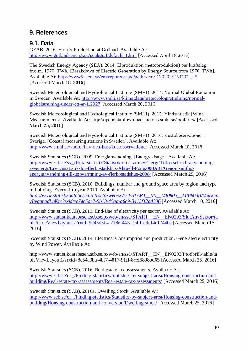
40
9. References
9.1. Data GEAB. 2016. Hourly Production at Gotland. Available At:
http://www.gotlandsenergi.se/geabgraf/default_1.htm [Accessed April 18 2016]
The Swedish Energy Agency (SEA). 2014. Elproduktion (nettoproduktion) per kraftslag
fr.o.m. 1970, TWh. [Breakdown of Electric Generation by Energy Source from 1970, TWh].
Available At: http://www5.stem.se/em/reports.aspx?path=/em/EN0202/EN0202_25
[Accessed March 18, 2016]
Swedish Meteorological and Hydrological Institute (SMHI). 2014. Normal Global Radiation
in Sweden. Available At: http://www.smhi.se/klimatdata/meteorologi/stralning/normal-
globalstralning-under-ett-ar-1.2927 [Accessed March 20, 2016]
Swedish Meteorological and Hydrological Institute (SMHI). 2015. Vindstatistik [Wind
Measurements]. Available At: http://opendata-download-metobs.smhi.se/explore/# [Accessed
March 25, 2016]
Swedish Meteorological and Hydrological Institute (SMHI). 2016. Kustobeservationer i
Sverige. [Coastal measuring stations in Sweden]. Available At:
http://www.smhi.se/vadret/hav-och-kust/kustobservationer [Accessed March 10, 2016]
Swedish Statistics (SCB). 2009. Energianvändning. [Energy Usage]. Available At:
http://www.scb.se/sv_/Hitta-statistik/Statistik-efter-amne/Energi/Tillforsel-och-anvandning-
av-energi/Energistatistik-for-flerbostadshus/Aktuell-Pong.008A01/Genomsnittlig-
energianvandning-till-uppvarmning-av-flerbostadshus-2008/ [Accessed March 25, 2016]
Swedish Statistics (SCB). 2010. Buildings, number and ground space area by region and type
of building. Every fifth year 2010. Available At:
http://www.statistikdatabasen.scb.se/pxweb/sv/ssd/START__MI__MI0803__MI0803B/Markan
vByggnadLnKn/?rxid=c7dc5ae7-9b13-45aa-a6c9-3415f12dd306 [Accessed March 10, 2016]
Swedish Statistics (SCB). 2013. End-Use of electricity per sector. Available At:
http://www.statistikdatabasen.scb.se/pxweb/en/ssd/START__EN__EN0203/SlutAnvSektor/ta
ble/tableViewLayout1/?rxid=9d46d3b4-718e-442a-94ff-d9df4c1744ba [Accessed March 15,
2016]
Swedish Statistics (SCB). 2014. Electrical Consumption and production. Generated electricity
by Wind Power. Available At:
http://www.statistikdatabasen.scb.se/pxweb/en/ssd/START__EN__EN0203/ProdbrEl/table/ta
bleViewLayout1/?rxid=8e54a0ba-4bf7-4817-91ff-8cef6898bd65 [Accessed March 25, 2016]
Swedish Statistics (SCB). 2016. Real-estate tax assessments. Available At:
http://www.scb.se/en_/Finding-statistics/Statistics-by-subject-area/Housing-construction-and-
building/Real-estate-tax-assessments/Real-estate-tax-assessments/ [Accessed March 25, 2016]
Swedish Statistics (SCB). 2016a. Dwelling Stock. Available At:
http://www.scb.se/en_/Finding-statistics/Statistics-by-subject-area/Housing-construction-and-
building/Housing-construction-and-conversion/Dwelling-stock/ [Accessed March 25, 2016]

41
Swedish Meteorological and Hydrological Institute (SMHI). 2012. STRÅNG-a Mesoscale
model for solar radiation. Available At: http://strang.smhi.se/ [Accessed March 25, 2016]
The Wind Power. 2016. Wind Turbines at Gotland. Available At:
http://www.thewindpower.net/zones_en_17_gotland.php [Accessed April 14, 2016]:
9.2. Literature Axelsson, U., Holm, A. & Liljegren, C., 1999. Gotland HVDC Light Transmission–World’s
first commercial small scale DC Transmission, CIRED Conferance Nice. (32).
Brito, M.C. et al., 2012. Photovoltaic potential in a Lisbon suburb using LiDAR data. Solar
Energy, 86(1), pp.283–288.
Brodén, D., 2013. Analysis of Demand Response Solutions for Congestion Management in
Distribution Networks. Master Thesis, Uppsala University.
Brundtland, G. et al., 1987. Our Common Future (Brundtland report), World Commission on
Environment and Development.
Buttler, A. et al., 2016. Variability of wind and solar power – An assessment of the current
situation in the European Union based on the year 2014. Energy, 106, pp.147–161.
Byman, K. & Nordling, J., 2016. Sveriges framtida elproduktion En delrapport [Swedens
future Electricity electricity generation, partial report, Stockholm: Kungliga
Ingenjörsakademin (IVA).
Camacho, E.F. et al., 2011. Control for Renewable Energy and Smart Grids. The Impact of
Control Technology, 1, pp.1–20.
Chen, C., 2011. Physics of solar energy, New Jersey: John Wiley & Sons.
Ekström, D., 2012. Gotlands solelpotential. Master Thesis, Uppsala University.
Energy Informative, 2016. Types of Solar Panels. Available at:
http://energyinformative.org/best-solar-panel-monocrystalline-polycrystalline-thin-film/
[Accessed April 10, 2016].
Gotland Energi AB, (GEAB), 2014. Wind Power Development. Available at:
http://www.gotlandsenergi.se/news.pab?nyhet=392 [Accessed April 5, 2016].
Gotlands Energi AB, (GEAB), 2016. Gotlands Elhistoria [History electrification Gotland].
Available at: URL: http://www.gotlandsenergi.se/historik.pab [Accessed April 11, 2016].
Ineichen, P., Guisan, O. & Perez, R., 1990. Ground-reflected radiation and albedo. Solar
Energy, 44(4), pp.207–214.
International Energy Agency (IEA), 2013. Sweden 2013. Energy Policies of IEA Countries,
Paris.
Jakubiec, J.A. & Reinhart, C.F., 2013. A method for predicting city-wide electricity gains
from photovoltaic panels based on LiDAR and GIS data combined with hourly Daysim
simulations. Solar Energy, 93, pp.127–143.
Jonsson, P. & Lindberg, F., 2011. Solar Energy from Existing Structures, Elforsk, report
11:77.

42
Kamp, S., 2013. Sveriges potential för elproduktion från takmonterade solceller. Master
Thesis Uppsala University.
Kjellsson, E., 2000. Potentialstudie för byggnadsintegrerade solceller i Sverige – Rapport 2.
Analys av instrålningsnivåer på byggnadsytor [Potential study of building mounted PV
power in Sweden], Lunds Tekniska Högskola, Report TVBH-7216.
Kupzog, F. et al., 2014. Maximising low voltage grid hosting capacity for PV and electric
mobility by distributed voltage control. Elektrotechnik und Informationstechnik, 131(6),
pp.188–192.
Lambert, Q., 2012. Business models for an aggregator-Information Management & Computer
Security, Master Thesis KTH.
Lantmäteriet, 2016. Facts about laser scanning. Available at:
https://www.lantmateriet.se/sv/Kartor-och-geografisk-information/Hojddata/Fakta-om-
laserskanning/ [Accessed March 18, 2016].
Lindahl, J., 2014. National Survey Report of PV Power Applications in SWEDEN 2014,
Swedish Energy Agency, Uppsala.
Lingfors, D. & Widén, J., 2014. Solenergipotentialen för Blekinges bebyggelse enligt två
framtids- scenarier [PV power potential in Blekinge County. Two future scenarios],
Länsstyrelsen Blekinge Län.
Mejia, F.A. & Kleissl, J., 2013. Soiling losses for solar photovoltaic systems in California.
Solar Energy, 95, pp.357–363.
Moren, G., 2013. Energimarknadsinspektionens föreskrifter och för att överföringen av el ska
vara av god kvalitet [Swedish Energy Market Inspectories rules for electricity
transmission quality], Energimarknadsinspektionens författningssamling,
Energimarknadsinspektionen, EIFS 2013:1, Eskilstuna.
Muñoz-García, M.A. et al., 2012. Characterization of thin film PV modules under standard
test conditions: Results of indoor and outdoor measurements and the effects of sunlight
exposure. Solar Energy, 86(10), pp.3049–3056.
van Noord, M. & Paradis, J., 2011. Solceller i samhällsplanering [PV power in community
planning], ELForsk, Report NR 11:75, Eskilstuna.
Nordpool, 2016. The Power Market. Available at: URL: http://www.nordpoolspot.com/How-
does-it-work/ [Accessed April 28, 2016].
Persson, T., 2000. Measurements-of-Solar-Radiation-in-Sweden-1983-1998, SMHI, Reports
Meteorology and Climatology, RMK No.89: SMHI.
PVsyst, 2016. Photovoltaic Software. Available at: http://www.pvsyst.com/en/ [Accessed
April 1, 2016].
Ramachandra, T. V. & Shruthi, B. V., 2007. Spatial mapping of renewable energy potential.
Renewable and Sustainable Energy Reviews, 11(7), pp.1460–1480.
Region Gotland, 2010. Energi, Infrastruktur och kommunikation [Energy Infrastructure and
communication], Visby.

43
Region Gotland, 2006. Energiplan för Ekokommun Gotland (Energy plan for Sustainable
Municipality Gotland), Visby.
Region Gotland, 2015. Gotland i siffror 2015 [Gotland in Numbers], Visby.
Region Gotland, 2011. Rapport från Gotlands Energidialog 2011 [Report from Gotland
energy dialog 2011], Visby.
Reilly, J. et al., 2015. Energy & Climate Outlook, MIT JOINT PROGRAM ON THE
SCIENCE AND POLICY OF GLOBAL CHANGE, Massachusetts.
Robèrt, K. et al., 2010. Strategic leadership towards sustainability, Blekinge Institute of
Technology: Karlshamn.
Rowlands, I.H., Kemery, B.P. & Beausoleil-Morrison, I., 2011. Optimal solar-PV tilt angle
and azimuth: An Ontario (Canada) case-study. Energy Policy, 39(3), pp.1397–1409.
Saga, T., 2010. Advances in crystalline silicon solar cell technology for industrial mass
production. NPG Asia Materials, 2(3), pp.96–102.
Sheffield, J., 1998. World population growth and the role of annual energy use per capita.
Technological forecasting and social change, 59(1), pp.55–87.
Sköldberg, H. et al., 2010. Ett fossilbränsleoberoende transportsystem år 2030 - Ett
visionsprojekt för Svensk Energi och Elforsk, Elforsk rapport 10:55.
Swedish Energy Agency (SEA), 2016. Delredovisning av uppdraget att ta fram ett förslag till
strategi för ökad användning av solel, Eskilstuna.
Swedish Energy Market Inspectorate (SEMI), 2015. Rättsfall mikroproducent [Micro
producer court in law]. , (2014-100203), pp.1–4.
Swedish Environmental Protection Agency (SEPA), 2016. Environmental objectives in
Sweden. Available at: http://www.miljomal.se/sv/Environmental-Objectives-
Portal/Undre-meny/About-the-Environmental-Objectives/ [Accessed April 15, 2016].
Svenska Kraftsnät (SVK), 2015. Anpassning av elsystemet med en stor mängd förnybar
elproduktion [Adjustment of the power system with a large amount of renewable
electricity], Slutrapport från Svenska Kraftsnät.
The Danish Wind Industry Association, 2003. Power control of Wind Turbines. Available at:
http://drømstørre.dk/wp-content/wind/miller/windpower web/en/tour/wtrb/powerreg.htm
[Accessed May 7, 2016].
The Swedish Energy Agency, (SEA), 2016. Stöd till solceller [Subsidy for PV systems).
Available at: http://www.energimyndigheten.se/fornybart/solenergi/stod-till-solceller/
[Accessed April 28, 2016].
The Swedish Tax Agency (STA), 2016. Skattereduktion för mikroproduction av förnyelsebar
el [Tax reduction for micro producersof renewable electricity production]. Available at:
http://www.skatteverket.se/privat/fastigheterbostad/mikroproduktionavfornybarel/skatter
eduktionformikroproduktionavfornybarel.4.12815e4f14a62bc048f4220.html?q=mikropr
oducent [Accessed March 30, 2016].
Uppsala University (UU), 2016. Thin-film Solar Cells. Available at:

44
http://www.teknik.uu.se/solid-state-electronics+/research-areas/solar-cells/ [Accessed
April 28, 2016].
Walla, T., 2012. Hosting capacity for photovoltaics in Swedish distribution grids. Master
Thesis Uppsala University.
Weiss, P. & Widén, J., 2012. Solenergi i Dalarnas bebyggelse Potential till år 2020 och 2050,
Länsstyrelsen i Dalarna, rapport 2012:05.
Wizelius, T., 2007. Developing wind power projects: theory and practice, London: Earthscan.
Yang, Y. & Bollen, M., 2008. Power quality and reliability in distribution networks with
increased levels of distributed generation. , (March), p.97. Available at:
https://www.etde.org/etdeweb/details.jsp?osti_id=941924.
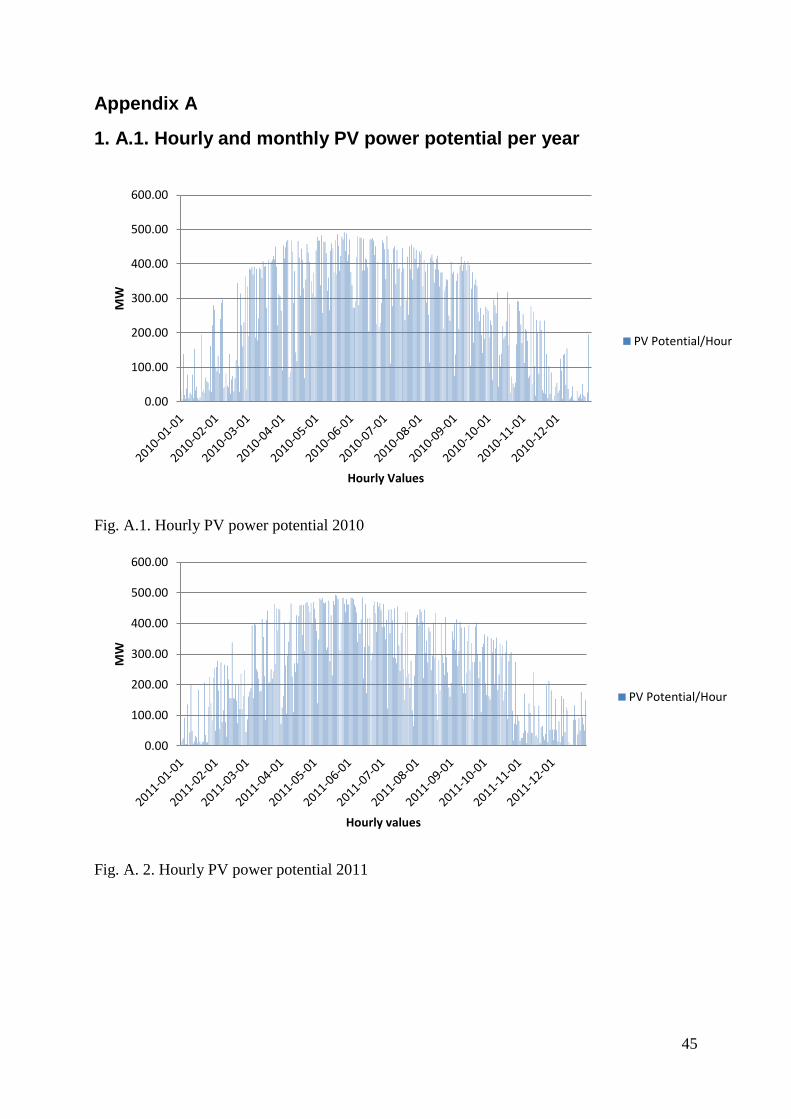
45
Appendix A
1. A.1. Hourly and monthly PV power potential per year
Fig. A.1. Hourly PV power potential 2010
Fig. A. 2. Hourly PV power potential 2011
0.00
100.00
200.00
300.00
400.00
500.00
600.00
MW
Hourly Values
PV Potential/Hour
0.00
100.00
200.00
300.00
400.00
500.00
600.00
MW
Hourly values
PV Potential/Hour

46
Fig. A. 5. Hourly PV power potential 2012.
0.00
100.00
200.00
300.00
400.00
500.00
600.00M
W
Hourly Values
PV Potential/Hour

47
A.2. Theoretical PV power potential for the different building categories Table. A. 1. Dwelling buildings PV power potential 2010-2012.
Dwelling Available
area after
reductions
m ²
Number of
buildings
Output
kW
Yearly
Production
kWh 2010
Yearly
Production
kWh 2011
Yearly
Production
kWh 2012
Type
Building
71 1 12 10543
10530
10545
Buildings
Total
1249174 17594 214338 185492258
185265293
185524389
Table. A. 2. Multi-Dwelling buildings PV power potential 2010-2012.
Multi
Dwelling
Roof type
Available
area after
reductions
m ²
Number of
Buildings
Output kW Yearly
Production
kWh 2010
Yearly
Production
kWh 2011
Yearly
Production
kWh 2012
Type
Building
Tilted
38 1
6
5564
5558
5565
Type
Building Flat
40 1
7
6973
6966
6973
Buildings
Total Tilted
322924 8498
51853
47282831
47224977
47291022
Buildings
Total Flat
60463 1499
10387
10455271
9863751
9873055
Total 383387 9977
62240
57738102
57088728
57164077
Table. A. 3. Industrial Buildings PV power potential 2010-2012.
Industry Available
area after
reductions.
m ²
Number
of
Buildings
Output kW Yearly
Production
kWh. 2010
Yearly
Production
kWh. 2011
Yearly
Production
kWh 2012
Type
Building
493 1
91
80502
80426
80502
Buildings
Total
233189 473
43543
38077552
38041621
38077506

48
Table. A. 4. Other Building PV power potential 2012-2012.
Other
Building
Roof Type
Available
area after
reductions.
m ²
Number
of
Buildings
Output kW Yearly
Production
kWh. 2010
Yearly
Production
kWh. 2011
Yearly
Production
kWh. 2012
Type
Building Tilt
46 1
8 6765
6757
6766
Type
Building Flat
52 1
8 7838
7831
7838
Building
Total Tilt
1348720 29320
222603 198351115
198108416
198385473
Building
Total Flat
1016392 19546
148396 153200469
153055906
153200283
Total 2365112 48866
370999
351551584
351164322
351585756

49
Appendix B
1. B Wind power simulation
Fig. B.1. Hourly production 2010.
Fig. B.2. Hourly Production 2011.
0
50
100
150
200
250
Ho
url
y V
alu
es
MW
2010
0
50
100
150
200
250
Ho
url
y P
rod
uct
ion
MW
2011

50
Fig. B. 3. Hourly Production 2012.
0
50
100
150
200
250H
ou
rly
Pro
du
ctio
n M
W
2012

51
Appendix C.
1. C. Figures and tables of the data material Table. C1. Global irradiance at Visby Measuring station 1999-2015 SMHI (2016).
Year Yearly Global Radiation kWh/m²
1999 1114
2000 1068
2001 1031
2002 1132
2003 1084
2004 1056
2005 1092
2006 1117
2007 1061
2008 1088
2009 1032
2010 902
2011 1026
2012 1028
2013 1091
2014 1092
2015 1106
Average year 1046
Fig. C. 1. Hourly wind speed at Fårösund measuring station 2012.
0
5
10
15
20
25
m/s
Hourly Values
Wind Speed Fårösund
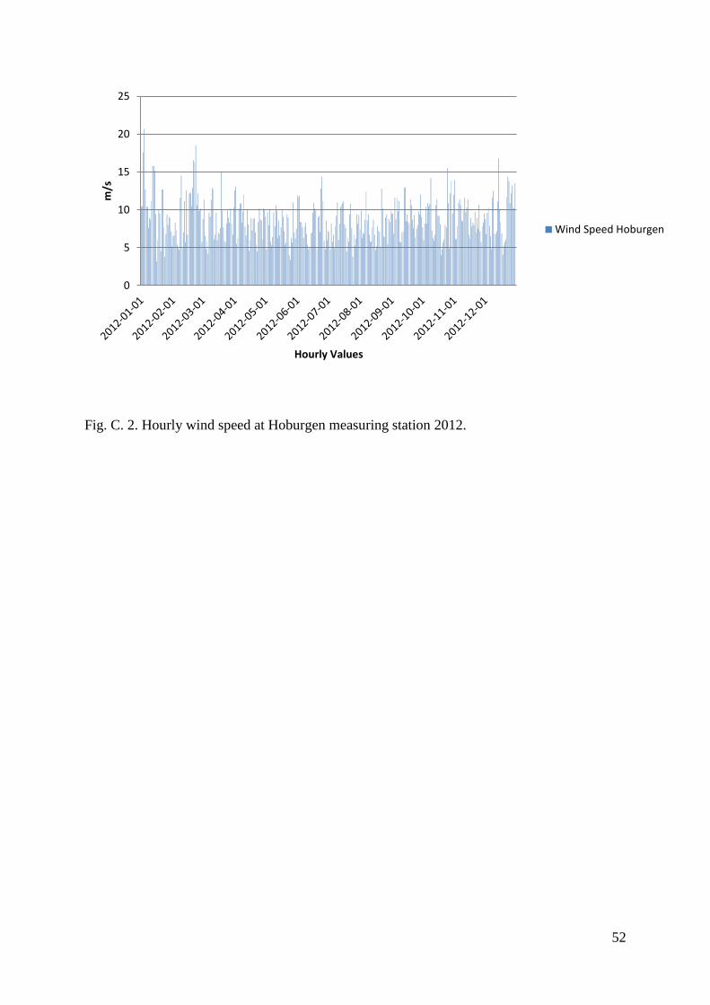
52
Fig. C. 2. Hourly wind speed at Hoburgen measuring station 2012.
0
5
10
15
20
25m
/s
Hourly Values
Wind Speed Hoburgen