Photoscopy: Spectroscopic Information from … Spectroscopic Information from Camera Snapshots? ... 1.3 Calculation of Pseudo Color Matching Functions ... 3 W UV LED (LED Engin) was

1

Photoscopy: Spectroscopic Information from Camera Snapshots?

Thimon Schwaebel,a Sebastian Menning,a Uwe H. F. Bunza,*

aOrganisch-Chemisches Institut, Ruprecht-Karls-Universität Heidelberg, Im Neuenheimer Feld 270, 69120

Heidelberg, FRG.

E-mail [email protected].

Supporting Information

Table of Content

1 Theory 2

1.1 Image Formation 2

1.2 Camera Behavior 2

1.3 Calculation of Pseudo Color Matching Functions (PCMF) 2

1.4 Identification of Primary Light Sources Using PCMF 3

2 Equipment and Materials 3

3 Dark Room Setup 4

4 Procedure: Calculation of PCMFs 5

4.1 Preliminary Work 5

4.2 Procedure to Determine Meta Data and Image Intensities (RGB values) 6

4.3 Calibration Procedure (390 - 710 nm, step size 10 nm) 9

4.4 Picture Processing 9

4.5 Spectra Processing 9

4.6 Calculation of the PCMFs 9

5 Procedure: Identification of Primary Light Sources Using PCMFs 9

5.1 Preliminary Work 9

5.2 Measurement 10

5.3 Processing of Pictures and Spectra 10

5.4 Calculation of the Chromaticity Coordinates 10

6 Additional Setups 10

7 RAW Data (camera behavior) 13

8 JPEG Data (camera behavior) 18

Electronic Supplementary Material (ESI) for Chemical ScienceThis journal is © The Royal Society of Chemistry 2013

mailto:[email protected]

2

1 Theory

1.1 Image Formation

The image intensity of a pixel is coupled to the spectral distribution and the spectral sensitivity or the pseudo color matching function (PCMF) of the camera. This is described by the following equation:

( ) ∫ ( ) ( )( ) (1)

I(k) refers to the image intensity, L(λ) is the radiance of the spectrum and S(k)(λ) is the PCMF. The exponent (k) stands for the three different color channels R (red), G (green) and B (blue). n is a constant referring to camera settings. The image intensity ranges from 0 to 65536 counts (16 bit color depth per channel).

1.2 Camera Behavior

To examine the behavior of the image intensity I(k) for each channel k (R, G, B), the white balance and all setup parameters (intensity of the incoming spectrum, distance, shutter speed, ISO value, f-number) were changed separately at three different wavelengths (450 nm, 550 nm 610 nm). The know formula for the irradiance of a picture1 could be confirmed for the data format RAW (see Figure S5 - Figure S15):

( )

( ) ∫ ( ) ( )( )

(

)

(2)

( )

(

)

(3)

L(λ) is the radiance of the recorded spectrum, t is the shutter speed, ISO is the ISO value, WB(k) is the factor of the white balance for the channel k, x is the distance between the origin of the radiance and the camera lens, N is the f-number and f is the focus point of the used lens. WB(k) is the only factor that is dependent on the color channel. Therefore normalized image intensities will be divided by that factor and the max value of color depth.

As a control we also analyzed the data for the picture format JPEG, but this behavior could not be found (see Figure S16 - Figure S26). Therefore JPEG image intensities are not suitable for statistical treatments and only the image intensities of RAW data were used to calculate the PCMFs. Still JPEG pictures give a good impression for the appearance of color and can be used to create arrays.

With this behavior in mind one can easily adjust the camera settings if the recorded light changes. For example if the spectrum will be one tenth of the intensity; the shutter speed or the ISO value can be deduced to get similar image intensity values.

1.3 Calculation of Pseudo Color Matching Functions (PCMF)

Converting Equation (1) in matrix notation we get:

(4)


3

I is a N x k matrix of the normalized image intensity values I(k) or RGB values (N refers to the amount of recorded images; k refers to the three color channels R, G and B), L is a N x W matrix of recorded monochromatic spectra L(λ) (W is the number of elements of the spectrum) and S is a W x k matrix of the camera PCMFs S(k)(λ).

When I and L are known S can be solved as followed:

(5)

L-1 is the inverse matrix of L. In order to compute L-1 correctly the rank of L needs to be N. Therefore the elements of the spectra are reduced to the amount of N being equal step sizes in the spectra.

Depending on the amount of images N, the PCMFs can be calculated in different step sizes. We decided to have a step size of 10 nm and a spectral range from 390 - 710 nm (N = 33).

1.4 Identification of Primary Light Sources Using PCMF

Using Equation (4) it is possible to use a spectrometer and a digital camera for identification. On the one hand chromaticity coordinates rg are recorded by the digital camera and on the other hand these are determined by a normalized emission spectrum L(λ) and the PCMFs S(k)(λ). It is necessary to work with chromaticity coordinates because relative or normalized spectra are used in the process to determine PCMFs or RGB values of the spectrum. Chromaticity coordinates rg are calculated from the normalized image intensity values I(k) as followed:

( )

( ) ( ) ( ) (6)

(̅ )

( ) ( ) ( ) (7)

The deviation Δ of the chromaticity coordinates of the image and the spectra will give the match. The deviation is calculated using this formula:

√( )

( )

(8)

2 Equipment and Materials

All organic dyes, quantum dot solutions, solvents and LEDs were purchased from commercially available sources; chemicals and solvents were used without purification. A 3 W UV LED (LED Engin) was used as an excitation source for the fluorescent solutions. To produce monochromatic light the excitation lamp and the monochromator of emission spectrometer (Jasco FP-6500, PTI QuantaMaster 40) were used. For reflecting the light a 20 x 20 cm TLC silica plate (Merck) or an Ulbricht sphere (Ø = 6’’; Labsphere) were used. All emission spectra were recorded using a Maya 2000 Pro CCD fiber spectrometer (Ocean Optics) which was corrected by wavelength and intensity. Photographs were taken with a Canon EOS 7D (objective: EF-S60mm f/2.8 Macro USM) using a focal aperture of F2.8, a film speed of ISO 100 - 400, a shutter speed of 0.1 – 0.25 s, a white balance of 5500K and a picture style of faithful. The photographs were saved in file format JPEG and RAW. The color space for the JPEG image was set to AdobeRGB 1998. RAW pictures were processed in


4

ImageJ 1.46r with plugin DCRaw Reader 1.3.0. The recorded image intensities have been calculated as mean values and standard deviations of a square at least 141 x 141 pixel. These values have been normalized. Adobe Illustrator CS5 was used to design the arrays.

3 Dark Room Setup

There are two different setups to determine PCMFs. One setup records the monochromatic light of the opening of an Ulbricht sphere (Setup I)2 and the other of a screen (Setup III or Setup IV; see Section 6)3. The spectrometer, FP-6500 and QuantaMaster 40, were only used to set the monochromators; these were controlled with a separate computer. The band pass of the monochromatic light was set to 5 nm. The digital camera and the CCD spectrometer were controlled with an additional computer. For all setups it was important that the camera and fiber were placed almost in the surface normal. When recording the picture and spectrum of the monochromatic light the room was.

Comparing all setups it is always to favor Setup I because the light is recorded directly and not from a reflected surface. This creates more reliable PCMFs.

Setup I (Figure S1): Using the lamp and the monochromator of the QuantaMaster 40 (PTI) equipped with an Ulbricht sphere. Band pass 5 nm.

Figure S1 Setup for the calibration of the camera with an Ulbricht sphere and the detection of the light from LEDs; A: overhead sketch; B: realistic setup. (1) Xenon lamp, (2) monochromator with a 1200 grid and two slits (S1 and S2), (3) sample compartment with two lenses (L) and a removable sample holder for LEDs (P), (4) Ulbricht sphere, (5) digital camera, (6) CCD fiber spectrometer, (7) laptop.


5

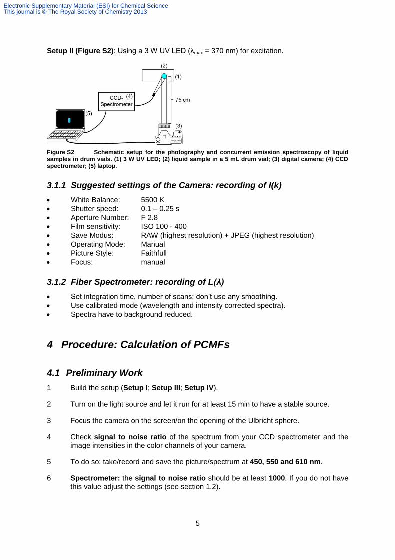
Setup II (Figure S2): Using a 3 W UV LED (λmax = 370 nm) for excitation.

Figure S2 Schematic setup for the photography and concurrent emission spectroscopy of liquid samples in drum vials. (1) 3 W UV LED; (2) liquid sample in a 5 mL drum vial; (3) digital camera; (4) CCD spectrometer; (5) laptop.

3.1.1 Suggested settings of the Camera: recording of I(k)

White Balance: 5500 K

Shutter speed: 0.1 – 0.25 s

Aperture Number: F 2.8

Film sensitivity: ISO 100 - 400

Save Modus: RAW (highest resolution) + JPEG (highest resolution)

Operating Mode: Manual

Picture Style: Faithfull

Focus: manual

3.1.2 Fiber Spectrometer: recording of L(λ)

Set integration time, number of scans; don’t use any smoothing.

Use calibrated mode (wavelength and intensity corrected spectra).

Spectra have to background reduced.

4 Procedure: Calculation of PCMFs

4.1 Preliminary Work

1 Build the setup (Setup I; Setup III; Setup IV).

2 Turn on the light source and let it run for at least 15 min to have a stable source.

3 Focus the camera on the screen/on the opening of the Ulbricht sphere.

4 Check signal to noise ratio of the spectrum from your CCD spectrometer and the image intensities in the color channels of your camera.

5 To do so: take/record and save the picture/spectrum at 450, 550 and 610 nm.

6 Spectrometer: the signal to noise ratio should be at least 1000. If you do not have this value adjust the settings (see section 1.2).


6

7 Camera: The image intensity value should be between 10000 and 30000 counts. If the image intensity value is too high or too low change the shutter speed or the ISO value. To determine the image intensity values follow the next steps.

4.2 Procedure to Determine Meta Data and Image Intensities (RGB

values)

8 Separate the JPEG and RAW pictures in two different folders.

9 Open the program: ImageJ.

10 Open path: Analyze/Set Measurements: check only Standard deviation, Mean gray value.

4.2.1 Determine Meta Data of RAW Images

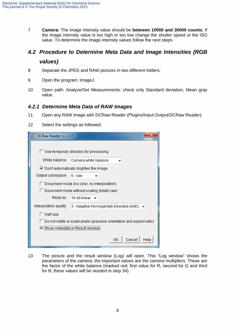
11 Open any RAW image with DCRaw Reader (Plugins/Input-Output/DCRaw Reader).

12 Select the settings as followed:

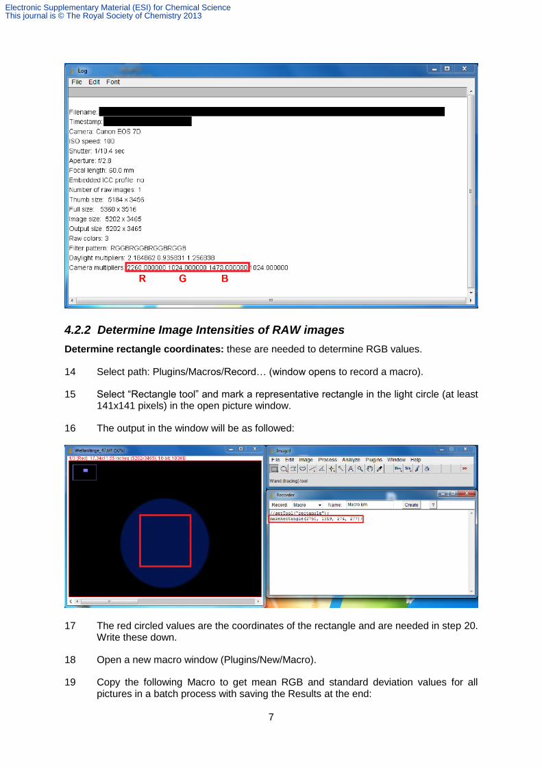
13 The picture and the result window (Log) will open. This “Log window” shows the parameters of the camera; the important values are the camera multipliers. These are the factor of the white balance (marked red; first value for R, second for G and third for B; these values will be needed in step 34).


7

4.2.2 Determine Image Intensities of RAW images

Determine rectangle coordinates: these are needed to determine RGB values.

14 Select path: Plugins/Macros/Record… (window opens to record a macro).

15 Select “Rectangle tool” and mark a representative rectangle in the light circle (at least 141x141 pixels) in the open picture window.

16 The output in the window will be as followed:

17 The red circled values are the coordinates of the rectangle and are needed in step 20. Write these down.

18 Open a new macro window (Plugins/New/Macro).

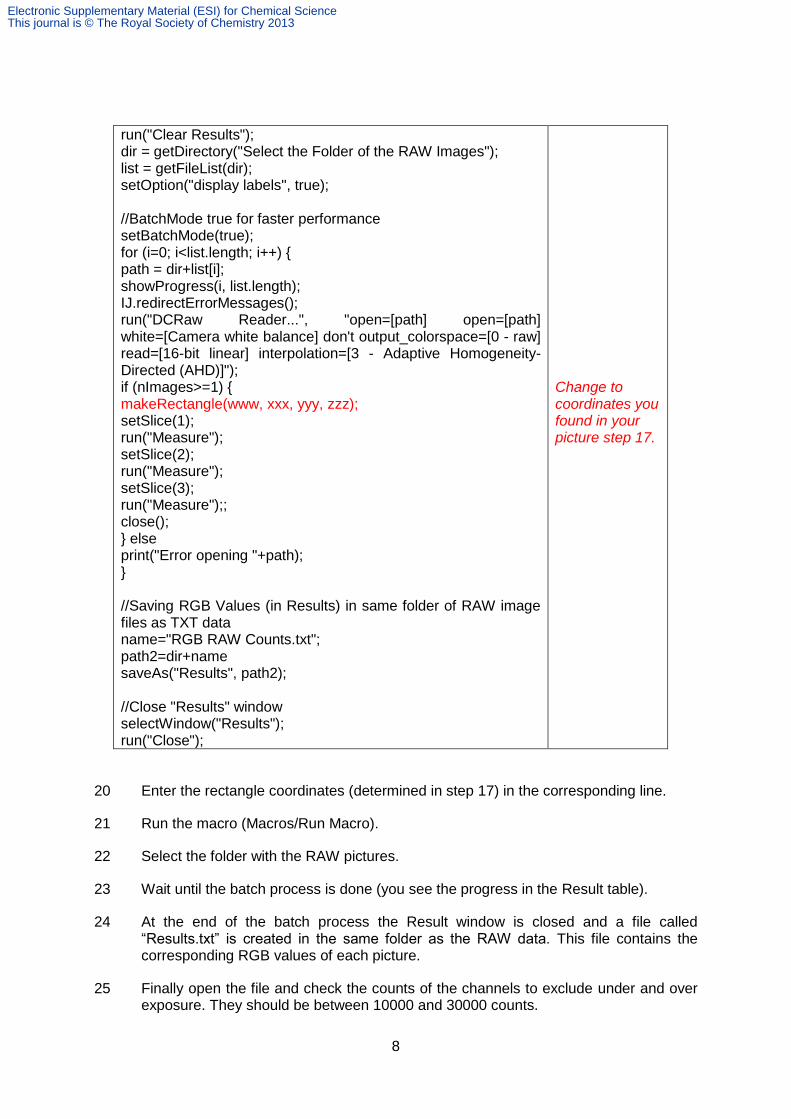
19 Copy the following Macro to get mean RGB and standard deviation values for all pictures in a batch process with saving the Results at the end:


8

run("Clear Results"); dir = getDirectory("Select the Folder of the RAW Images"); list = getFileList(dir); setOption("display labels", true); //BatchMode true for faster performance setBatchMode(true); for (i=0; i<list.length; i++) { path = dir+list[i]; showProgress(i, list.length); IJ.redirectErrorMessages(); run("DCRaw Reader...", "open=[path] open=[path] white=[Camera white balance] don't output_colorspace=[0 - raw] read=[16-bit linear] interpolation=[3 - Adaptive Homogeneity-Directed (AHD)]"); if (nImages>=1) { makeRectangle(www, xxx, yyy, zzz); setSlice(1); run("Measure"); setSlice(2); run("Measure"); setSlice(3); run("Measure");; close(); } else print("Error opening "+path); } //Saving RGB Values (in Results) in same folder of RAW image files as TXT data name="RGB RAW Counts.txt"; path2=dir+name saveAs("Results", path2); //Close "Results" window selectWindow("Results"); run("Close");

Change to coordinates you found in your picture step 17.

20 Enter the rectangle coordinates (determined in step 17) in the corresponding line.

21 Run the macro (Macros/Run Macro).

22 Select the folder with the RAW pictures.

23 Wait until the batch process is done (you see the progress in the Result table).

24 At the end of the batch process the Result window is closed and a file called “Results.txt” is created in the same folder as the RAW data. This file contains the corresponding RGB values of each picture.

25 Finally open the file and check the counts of the channels to exclude under and over exposure. They should be between 10000 and 30000 counts.


9

4.3 Calibration Procedure (390 - 710 nm, step size 10 nm)

26 Change monochromator wavelength to 390 nm.

27 Take/Record and save the picture and spectrum of each monochromatic light.

28 Repeat steps 26 and 27 for every 10 nm until 710 nm are reached.

29 Take and save the last picture without any light (background); no spectrum is required.

4.4 Picture Processing

30 Follow the procedure to save the “Results.txt”-file of the monochromatic light (steps 8 - 24).

4.5 Spectra Processing

31 The emission spectra need to be in the range from 390 to 710 nm with a 10 nm step size.

4.6 Calculation of the PCMFs

32 Open the attached Excel file “PCMFs.xlsm”.

33 Copy the RGB values from the saved Results (step 30) into the sheet “Monochromatic RGB Values” Column A – D.

34 Enter the settings of the white balance in the cells (H38, H39, H40) (step 13).

35 Activate the macro “change_order”.

36 Copy the spectra (from step 31) into the sheet “Monochromatic Spectra”.

37 The calculation is done automatically.

38 The PCMFs will be in the sheet “PCMFs” column “AU – AW” (see graph).

39 Save the file.

5 Procedure: Identification of Primary Light Sources

Using PCMFs

5.1 Preliminary Work

40 Build the Setup II.

41 Prepare the fluorescent solution in 5mL drum vials.

42 Place the vial on the excitation lamp.

43 Focus the camera on the vial.


10

44 Check the intensity of the spectrum and the image intensity of the color channels (see steps 6 - 25).

5.2 Measurement

45 Record the vial with the digital camera and the fiber spectrometer in a dark room (or just take the photograph, if the spectrum is already known).

46 Record a picture of the background.

5.3 Processing of Pictures and Spectra

47 Follow the procedure to determine RGB values (steps 8 - 24) and to process emission spectra (step 31).

5.4 Calculation of the Chromaticity Coordinates

48 Open the Excel file with the PCMFs “PCMFs.xlsm” from the steps 32 - 39.

5.4.1 Image

49 Copy the RGB values from the saved Results (step 47) into the sheet “RGB Values” Column A – D.

50 Enter the white balance settings into the cells (H18, H19, H20) (step 13).

51 Activate the macro “change_order”.

52 Put the values of the background in the corresponding background cells.

53 The chromaticity coordinates will appear in column S and T.

5.4.2 Spectra

54 Copy the emission spectra (step 47) into the sheet “Spectra”.

55 The chromaticity coordinates will appear in column W and X.

5.4.3 Deviation

56 The deviation will appear in the sheet “Deviation”.

6 Additional Setups

Building a self-made reflectance screen: To build a screen use a 20 x 20 cm TLC plate and glue it on a piece of cardboard.

Setup III (Figure S 3): Using the lamp and the monochromator of the FP-6500 (Jasco) producing a light spot on a self-made screen (TLC plate). Band pass 5 nm.

Setup IV (Figure S 4): Using the lamp and the monochromator of the Quantamaster 40 (PTI) producing a light spot on a self-made screen (TLC plate). Band pass 5 nm.


11

Figure S3 Setup for the calibration of the camera with a self-made screen; A: overhead sketch; B: realistic setup. (1) FP-6500 spectrometer (Jasco), (2) self-made screen, (3) digital camera, (4) CCD fiber spectrometer, (5) laptop.


12

Figure S4 Setup for the calibration of the camera with a self-made screen; A: overhead sketch; B: realistic setup. (1) Xenon lamp, (2) monochromator with a 1200 grid and two slits (S1 and S2), (3) sample compartment with two lenses (L) and a removable sample holder for LEDs (P), (4) self-made screen, (5) digital camera, (6) CCD fiber spectrometer, (7) laptop.


13

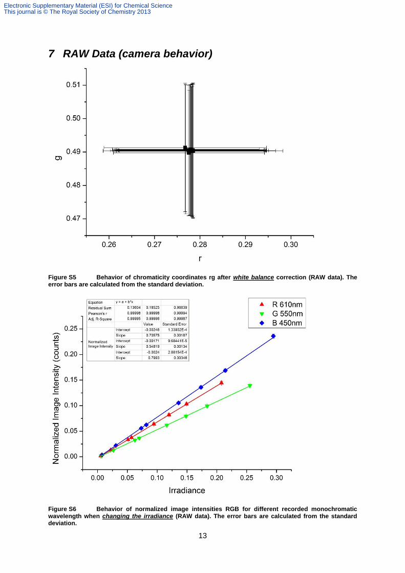
7 RAW Data (camera behavior)

Figure S5 Behavior of chromaticity coordinates rg after white balance correction (RAW data). The error bars are calculated from the standard deviation.

Figure S6 Behavior of normalized image intensities RGB for different recorded monochromatic wavelength when changing the irradiance (RAW data). The error bars are calculated from the standard deviation.


14

Figure S7 Behavior of chromaticity coordinates rg for different recorded monochromatic wavelength when changing the irradiance (RAW data). The error bars are calculated from the standard deviation.

Figure S8 Behavior of image intensities RGB for different recorded monochromatic wavelength when changing the distance (RAW data).


15

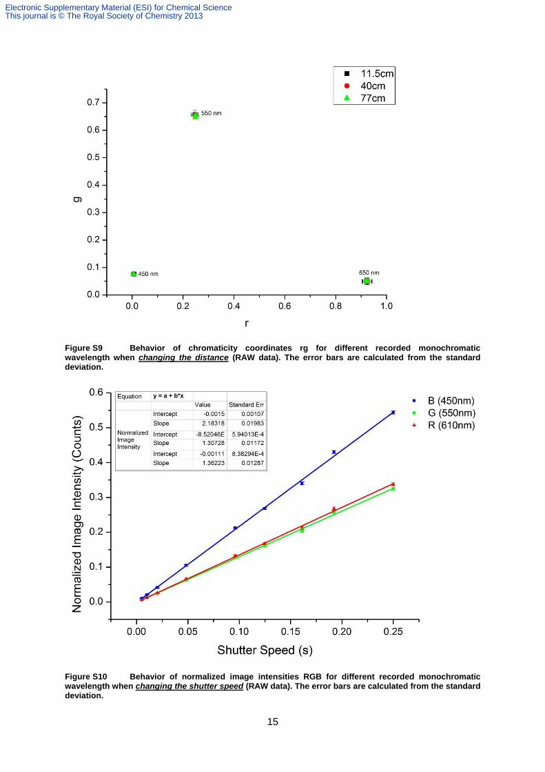
Figure S9 Behavior of chromaticity coordinates rg for different recorded monochromatic wavelength when changing the distance (RAW data). The error bars are calculated from the standard deviation.

Figure S10 Behavior of normalized image intensities RGB for different recorded monochromatic wavelength when changing the shutter speed (RAW data). The error bars are calculated from the standard deviation.


16

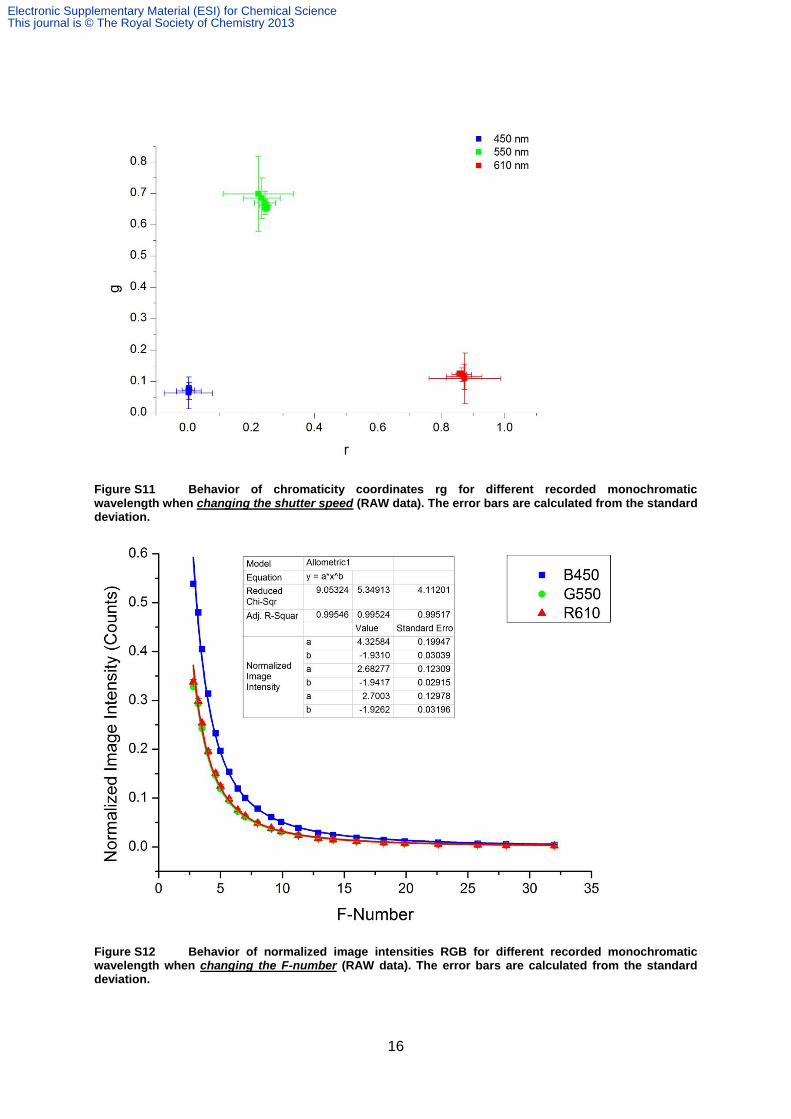
Figure S11 Behavior of chromaticity coordinates rg for different recorded monochromatic wavelength when changing the shutter speed (RAW data). The error bars are calculated from the standard deviation.

Figure S12 Behavior of normalized image intensities RGB for different recorded monochromatic wavelength when changing the F-number (RAW data). The error bars are calculated from the standard deviation.


17

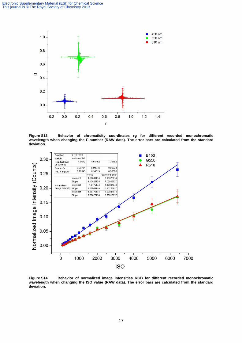
Figure S13 Behavior of chromaticity coordinates rg for different recorded monochromatic wavelength when changing the F-number (RAW data). The error bars are calculated from the standard deviation.

Figure S14 Behavior of normalized image intensities RGB for different recorded monochromatic wavelength when changing the ISO value (RAW data). The error bars are calculated from the standard deviation.


18

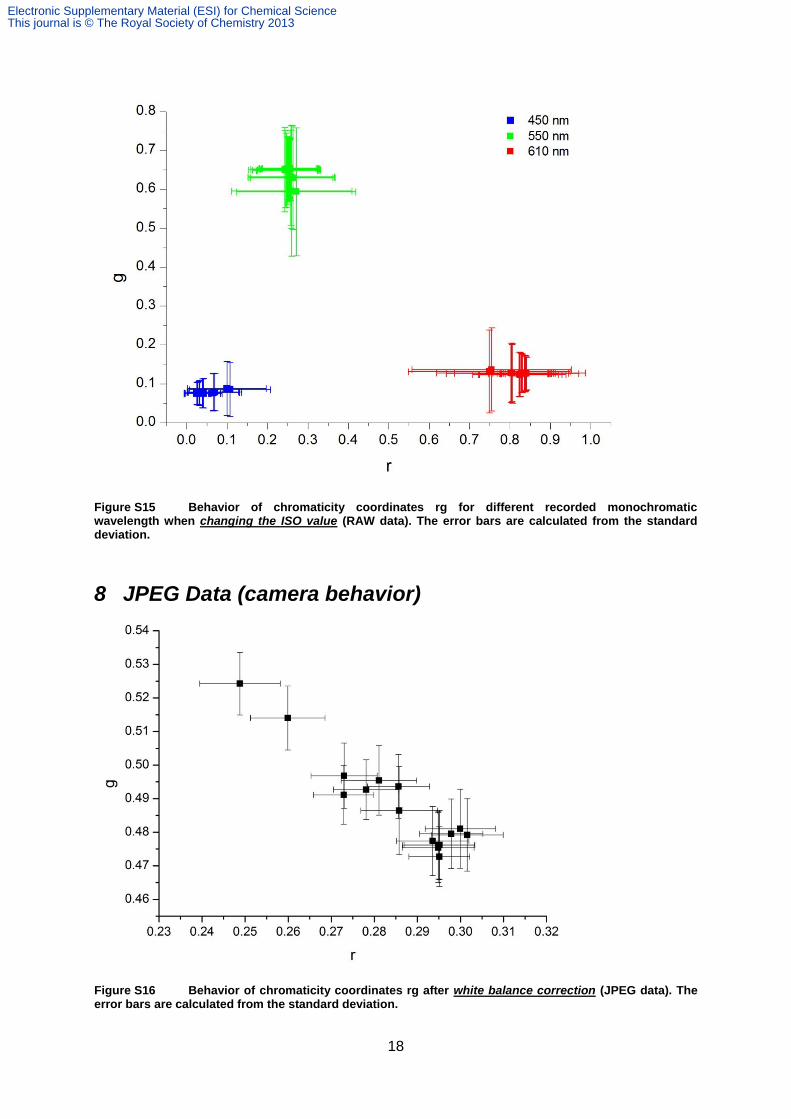
Figure S15 Behavior of chromaticity coordinates rg for different recorded monochromatic wavelength when changing the ISO value (RAW data). The error bars are calculated from the standard deviation.

8 JPEG Data (camera behavior)

Figure S16 Behavior of chromaticity coordinates rg after white balance correction (JPEG data). The error bars are calculated from the standard deviation.


19

Figure S17 Behavior of normalized image intensities RGB for different recorded monochromatic wavelength when changing the irradiance (JPEG data). The error bars are calculated from the standard deviation.

Figure S18 Behavior of chromaticity coordinates rg for different recorded monochromatic wavelength when changing the irradiance (JPEG data). The error bars are calculated from the standard deviation.


20

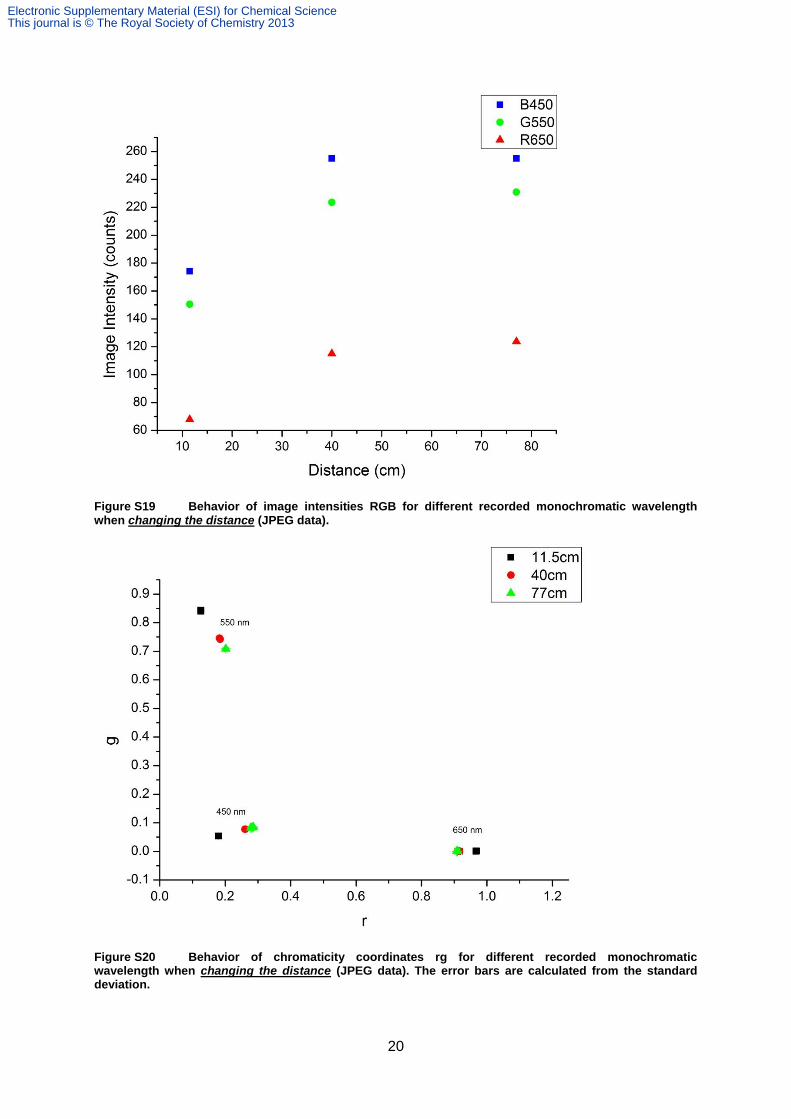
Figure S19 Behavior of image intensities RGB for different recorded monochromatic wavelength when changing the distance (JPEG data).

Figure S20 Behavior of chromaticity coordinates rg for different recorded monochromatic wavelength when changing the distance (JPEG data). The error bars are calculated from the standard deviation.


21

Figure S21 Behavior of normalized image intensities RGB for different recorded monochromatic wavelength when changing the shutter speed (JPEG data). The error bars are calculated from the standard deviation.

Figure S22 Behavior of chromaticity coordinates rg for different recorded monochromatic wavelength when changing the shutter speed (JPEG data). The error bars are calculated from the standard deviation.


22

Figure S23 Behavior of normalized image intensities RGB for different recorded monochromatic wavelength when changing the F-number (JPEG data). The error bars are calculated from the standard deviation.

Figure S24 Behavior of chromaticity coordinates rg for different recorded monochromatic wavelength when changing the F-number (JPEG data). The error bars are calculated from the standard deviation.


23

Figure S25 Behavior of normalized image intensities RGB for different recorded monochromatic wavelength when changing the ISO value (JPEG data). The error bars are calculated from the standard deviation.

Figure S26 Behavior of chromaticity coordinates rg for different recorded monochromatic wavelength when changing the ISO value (JPEG data). The error bars are calculated from the standard deviation.


24

Figure S27 Pseudo color matching function of the camera Canon EOS 7D determined by using Setup III.

Figure S28 Pseudo color matching function of the camera Canon EOS 7D determined by using Setup IV.


25

1 Michael Bass (1995), Handbooks of Optics Volume II: Devices, Measurements and Properties, 2

nd

edition, McGraw-Hill Inc., chapter 24. 2 Sigernes, F.; Dyrland, M.; Peters, N.; Lorentzen, D. A.; Svenøe, T.; Heia, K.; Chernouss, S.; Deehr,

C. S.; Kosch, M. Opt. Express 2009, 17, 20211-20220. 3 Sigernes, F.; Holmes, J. M.; Dyrland, M.; Lorentzen, D. A.; Svenøe, T.;. Heia, K; Aso, T.; Chernouss,

S.; Deehr, C. S. Opt. Express 2008, 16, 15623-15632.


Documents

Photoscopy: Spectroscopic Information from … Spectroscopic Information from Camera Snapshots? ... 1.3 Calculation of Pseudo Color Matching Functions ... 3 W UV LED (LED Engin) was