Photonic modes in colloidal / complex nematic resonators

Iztok BajcFrédéric Hecht

Slobodan Žumer

Fakulteta

za

matematiko

in

fizikoUniverza

v

Ljubljani

Slovenija

Outline

•

Nematic liquid crystals - properties•

Motivational nematic photonic systems

•

Computational methods•

Example: EM eigen modes in a nematic system

•

Possible further work

Low enoughtemperature

Isotropic liquid phase(higher temperature)

•

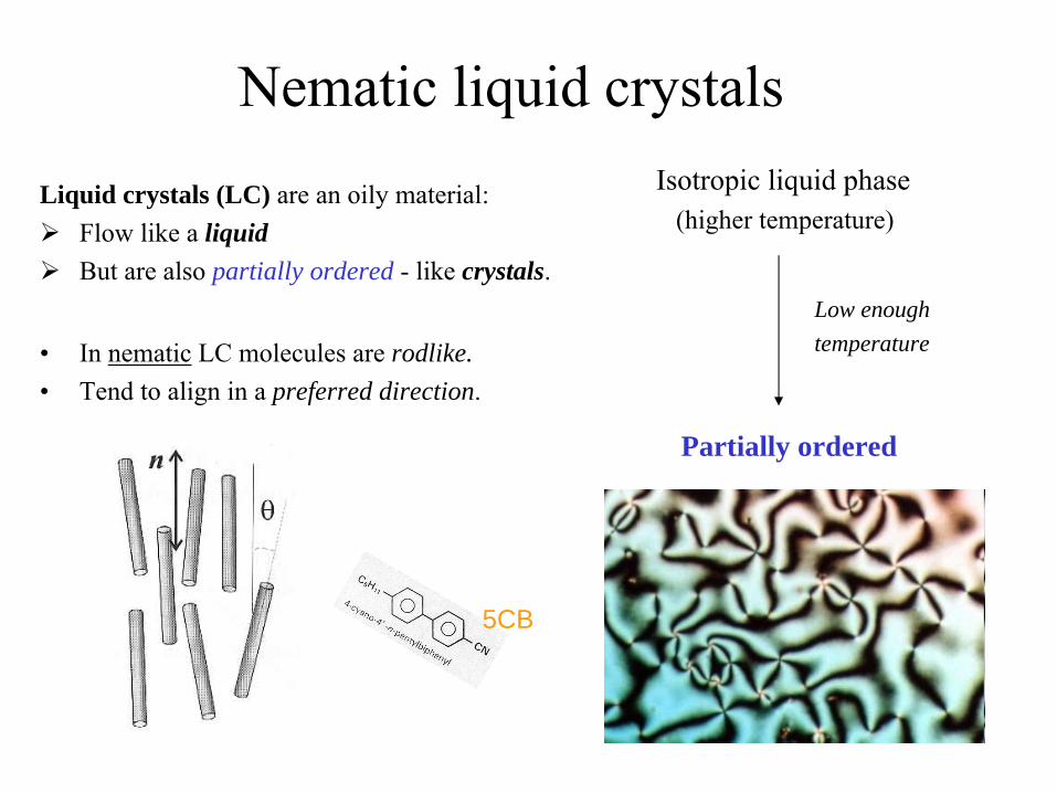
In nematic

LC molecules are

rodlike.•

Tend to align in a preferred direction.

Partially ordered

5CB

Liquid crystals (LC) are an oily material:

Flow like a liquid

But are also partially ordered - like crystals.

Nematic liquid crystals

3×3×3 dipolar crystal.Experiment by Andriy Nych,2012 (submitted).

Larger 3Dstructures

Nematic photonic crystals

(Recently built also 6×6×6)

Motivational system 1:

Nematic and chiral nematic droplets

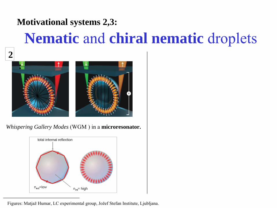
Figures: Matjaž

Humar, LC experimental group, Jožef Stefan Institute, Ljubljana.

Whispering Gallery Modes (WGM ) in a microresonator.

Motivational systems 2,3:

2 :

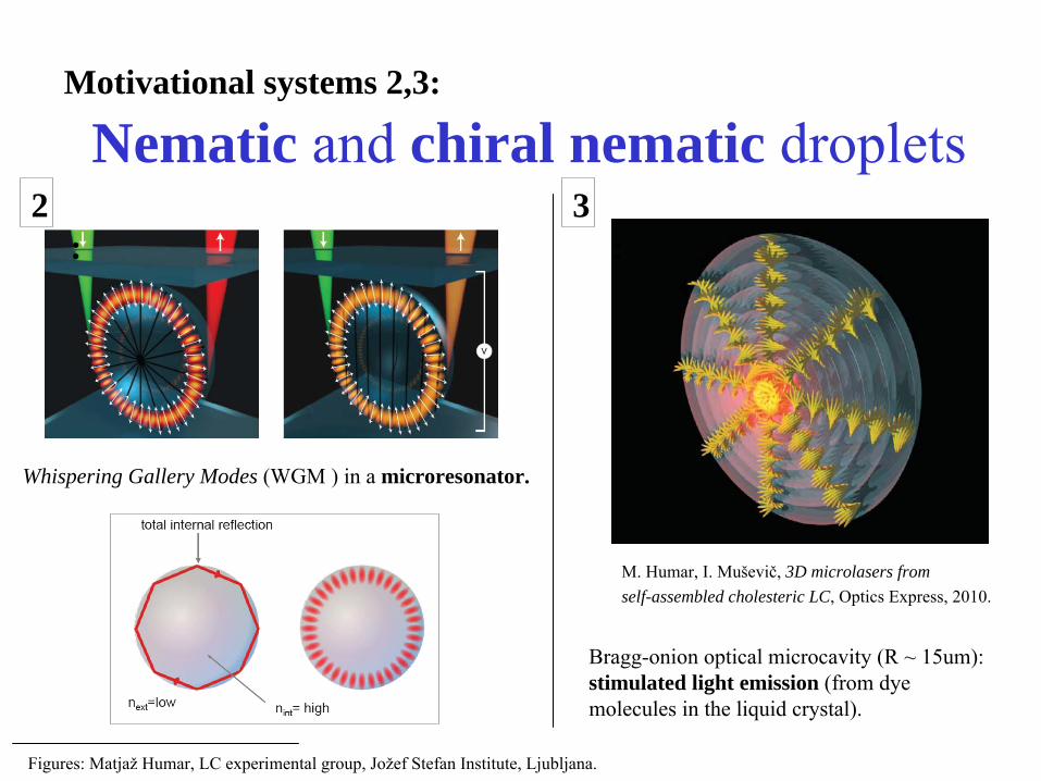
Nematic and chiral nematic droplets

Figures: Matjaž

Humar, LC experimental group, Jožef Stefan Institute, Ljubljana.

Whispering Gallery Modes (WGM ) in a microresonator.

Bragg-onion optical microcavity (R ~ 15um): stimulated light emission (from dye molecules in the liquid crystal).

M. Humar,

I. Muševič, 3D microlasers from self-assembled cholesteric LC, Optics Express, 2010.

2 :

3 :

Motivational systems 2,3:

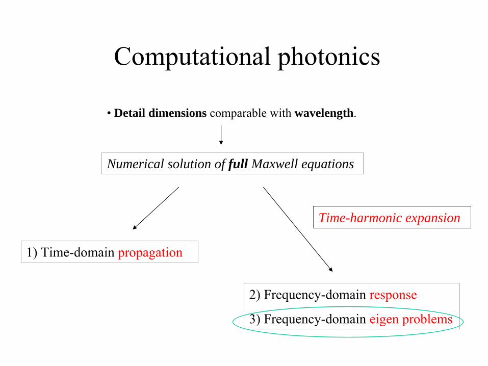
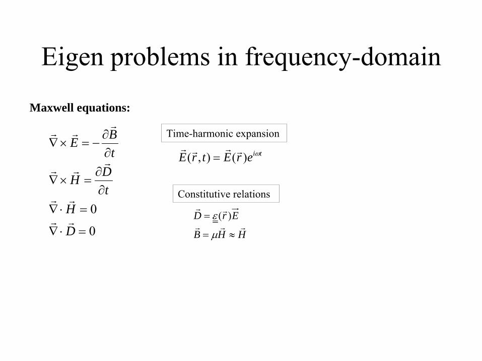
Time-harmonic expansion

Computational photonics

2) Frequency-domain response

3) Frequency-domain eigen problems

• Detail dimensions comparable with wavelength.

Numerical solution of full Maxwell equations

1) Time-domain propagation

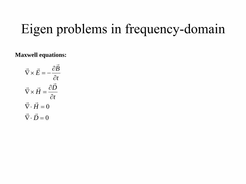
Eigen problems in frequency-domain

0

0

D

HtDH

tBE

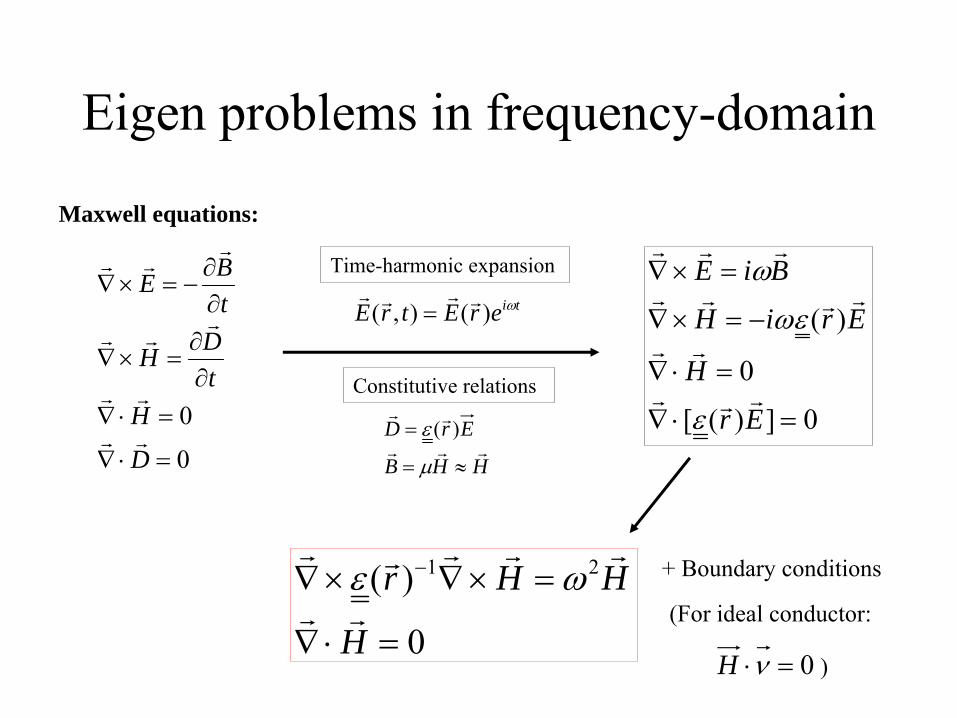
Maxwell equations:

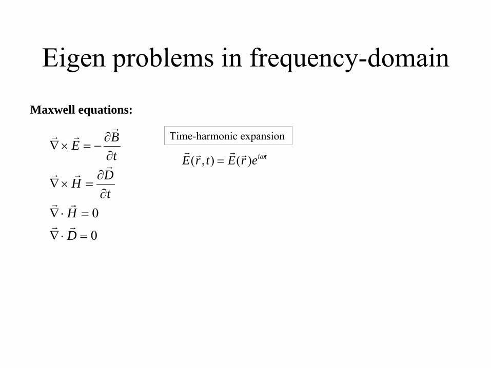
Eigen problems in frequency-domain

0

0

D

HtDH

tBE

Time-harmonic expansion

tierEtrE )(),(

Maxwell equations:

Eigen problems in frequency-domain

0

0

D

HtDH

tBE

HHB

ErD

)(

Time-harmonic expansion

Constitutive relations

tierEtrE )(),(

Maxwell equations:

Eigen problems in frequency-domain

0

0

D

HtDH

tBE

HHB

ErD

)( 0])([

0

)(

Er

H

EriH

BiE

Time-harmonic expansion

Constitutive relations

tierEtrE )(),(

Maxwell equations:

Eigen problems in frequency-domain

0

0

D

HtDH

tBE

0H0

)( 21

H

HHr

(For ideal conductor:

HHB

ErD

)(

Time-harmonic expansion

Constitutive relations

tierEtrE )(),(

+ Boundary conditions

)

Maxwell equations:

0])([

0

)(

Er

H

EriH

BiE

Eigen problems in frequency-domain

0

0

D

HtDH

tBE

0H0

)( 21

H

HHr

(For ideal conductor:

HHB

ErD

)(

Time-harmonic expansion

Constitutive relations

tierEtrE )(),(

+ Boundary conditions

)

Maxwell equations:

0])([

0

)(

Er

H

EriH

BiE

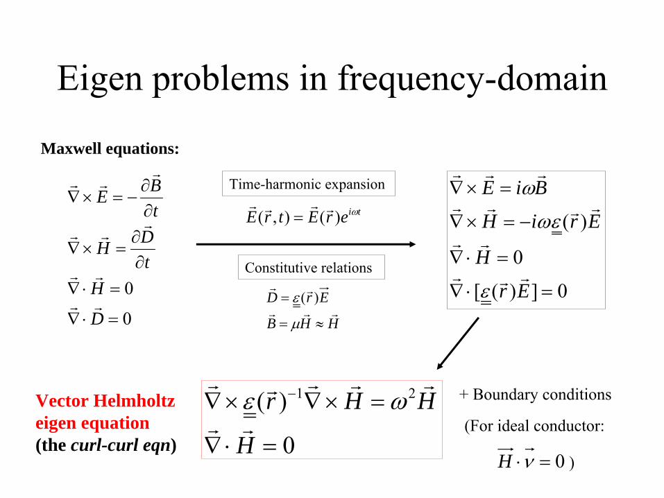
Vector Helmholtz eigen equation (the curl-curl eqn)

Eigen problems in frequency-domain

0

0

D

HtDH

tBE

0H0

)( 21

H

HHr

(For ideal conductor:

HHB

ErD

)(

Time-harmonic expansion

Constitutive relations

tierEtrE )(),(

+ Boundary conditions

)

Maxwell equations:

0])([

0

)(

Er

H

EriH

BiE

Vector Helmholtz eigen equation (the curl-curl eqn)

Fully anisotropic permittivity

Helmholtz and Schroedinger eqns

Helmholtz and Schroedinger eqns

HHr

21)(

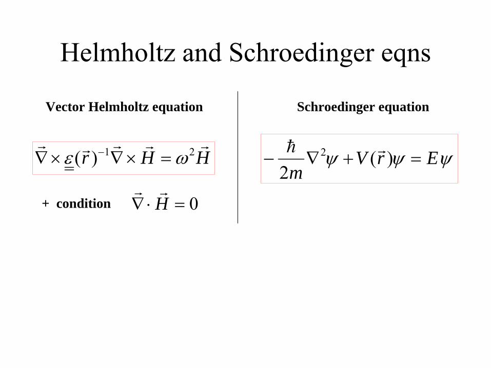
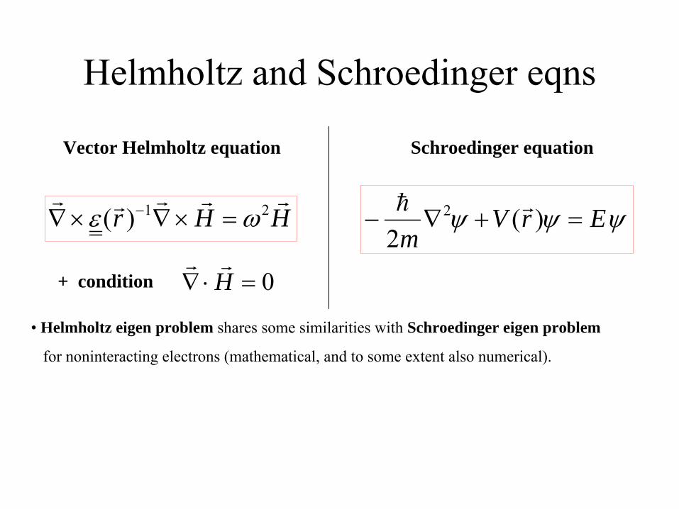
Vector Helmholtz equation

ErVm

)(2

2

Schroedinger equation

0 H

+ condition

Helmholtz and Schroedinger eqns

HHr

21)(

Vector Helmholtz equation

ErVm

)(2

2

Schroedinger equation

0 H

+ condition

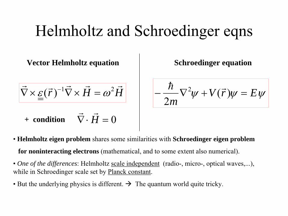
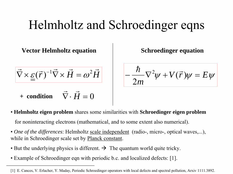
• Helmholtz eigen problem shares some similarities with Schroedinger eigen problem

for noninteracting electrons (mathematical, and to some extent also numerical).

Helmholtz and Schroedinger eqns

HHr

21)(

Vector Helmholtz equation

ErVm

)(2

2

Schroedinger equation

0 H

+ condition

• Helmholtz eigen problem shares some similarities with Schroedinger eigen problem

for noninteracting electrons (mathematical, and to some extent also numerical).

•

One of the differences: Helmholtz scale independent

(radio-, micro-, optical waves,...), while in Schroedinger scale set by Planck constant.

Helmholtz and Schroedinger eqns

HHr

21)(

Vector Helmholtz equation

ErVm

)(2

2

Schroedinger equation

0 H

+ condition

• Helmholtz eigen problem shares some similarities with Schroedinger eigen problem

for noninteracting electrons (mathematical, and to some extent also numerical).

•

One of the differences: Helmholtz scale independent

(radio-, micro-, optical waves,...), while in Schroedinger scale set by Planck constant.

• But the underlying physics is different.

The quantum world quite tricky.

Helmholtz and Schroedinger eqns

HHr

21)(

Vector Helmholtz equation

ErVm

)(2

2

Schroedinger equation

0 H

+ condition

• Helmholtz eigen problem shares some similarities with Schroedinger eigen problem

for noninteracting electrons (mathematical, and to some extent also numerical).

•

One of the differences: Helmholtz scale independent

(radio-, micro-, optical waves,...), while in Schroedinger scale set by Planck constant.

• But the underlying physics is different.

The quantum world quite tricky.

• Example of Schroedinger eqn with periodic b.c. and localized defects: [1].

[1] E. Cances, V. Erlacher, Y. Maday, Periodic Schroedinger operators with local defects and spectral pollution, Arxiv 1111.3892.

Formulation and numerics for Helmholtz

Formulation and numerics for Helmholtz

[2] J.C. Nedelec, Mixed Finite Elements in R^3, Numer. Math. 35, 315 -

341 (1980). [1] A.

Bossavit, Computational Electromagnetism, Academic Press, 1998.

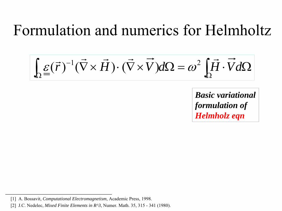
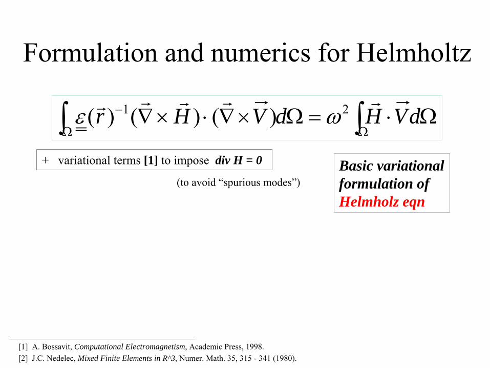
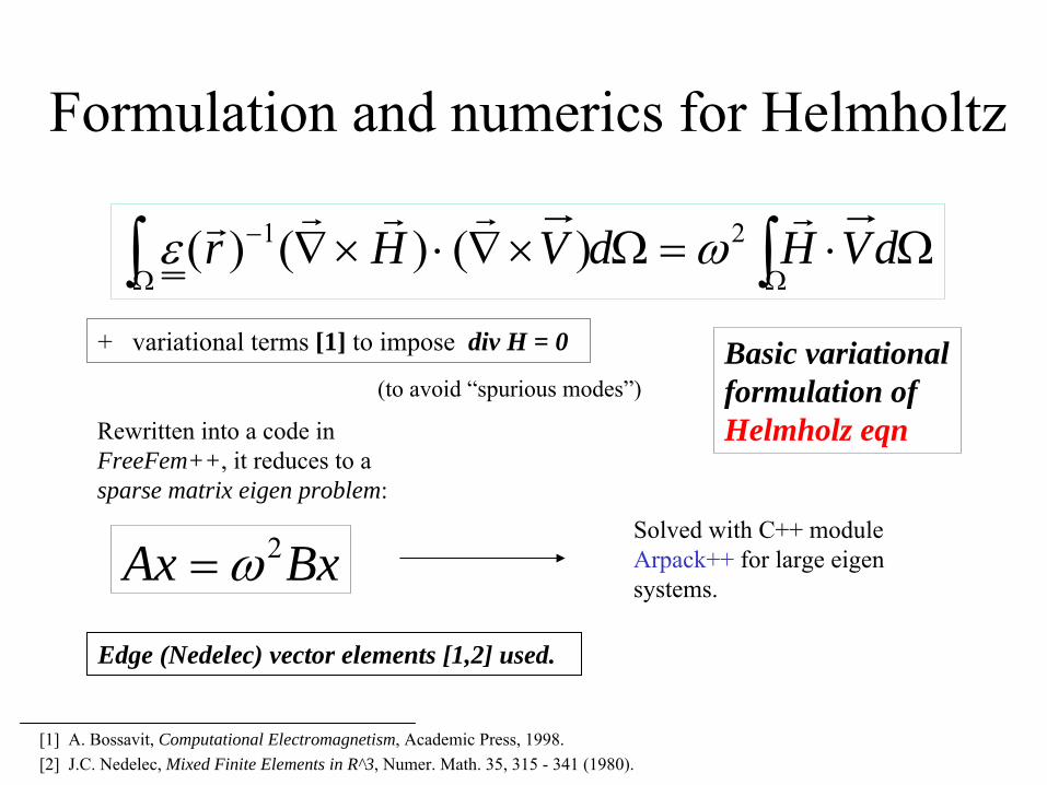
dVHdVHr 21 )()()(

Basic variational formulation of Helmholz eqn

Formulation and numerics for Helmholtz

[2] J.C. Nedelec, Mixed Finite Elements in R^3, Numer. Math. 35, 315 -

341 (1980). [1] A.

Bossavit, Computational Electromagnetism, Academic Press, 1998.

dVHdVHr 21 )()()(

Basic variational formulation of Helmholz eqn

+ variational terms [1] to impose div H = 0

(to avoid “spurious modes”)

Formulation and numerics for Helmholtz

[2] J.C. Nedelec, Mixed Finite Elements in R^3, Numer. Math. 35, 315 -

341 (1980). [1] A.

Bossavit, Computational Electromagnetism, Academic Press, 1998.

Rewritten into a code in FreeFem++, it reduces to a sparse matrix eigen problem:

BxAx 2Solved with C++ module Arpack++ for large eigen systems.

dVHdVHr 21 )()()(

Basic variational formulation of Helmholz eqn

+ variational terms [1] to impose div H = 0

(to avoid “spurious modes”)

Formulation and numerics for Helmholtz

[2] J.C. Nedelec, Mixed Finite Elements in R^3, Numer. Math. 35, 315 -

341 (1980). [1] A.

Bossavit, Computational Electromagnetism, Academic Press, 1998.

Rewritten into a code in FreeFem++, it reduces to a sparse matrix eigen problem:

BxAx 2Solved with C++ module Arpack++ for large eigen systems.

dVHdVHr 21 )()()(

Basic variational formulation of Helmholz eqn

+ variational terms [1] to impose div H = 0

(to avoid “spurious modes”)

Edge (Nedelec) vector elements [1,2] used.

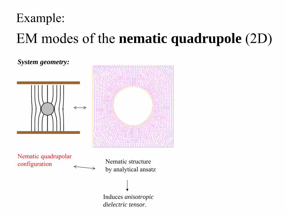
EM modes of the nematic quadrupole (2D)

Nematic quadrupolar configuration

System geometry:

Example:

EM modes of the nematic quadrupole (2D)

Nematic quadrupolar configuration

System geometry:

Example:

Induces anisotropic dielectric tensor.

Nematic structure

by analytical ansatz

EM modes of the nematic quadrupole (2D)

Nematic quadrupolar configuration Nematic structure

by analytical ansatz

2D mesh: ~5000 vertices

System geometry:

Example:

Induces anisotropic dielectric tensor.

EM modes of the nematic quadrupole (2D)

Nematic quadrupolar configuration Nematic structure

by analytical ansatz

System geometry:

Example:

Induces anisotropic dielectric tensor.

We compute EM modes on this nematic structure

2D mesh: ~5000 vertices

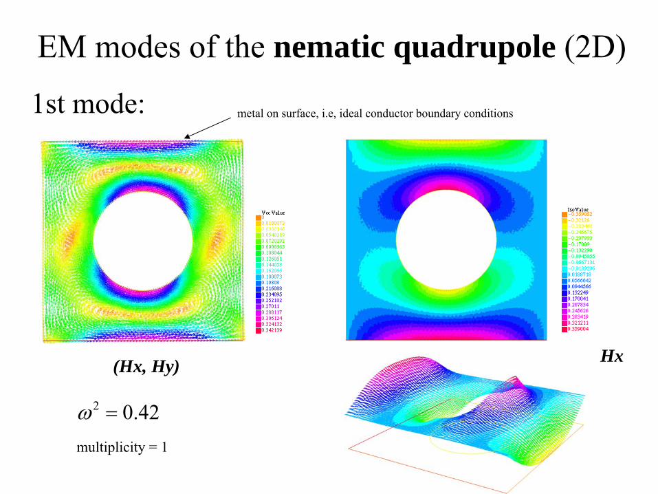
EM modes of the nematic quadrupole (2D)

(Hx, Hy)

1st mode:

Hx

multiplicity = 1

42.02

metal on surface, i.e, ideal conductor boundary conditions

(Hx, Hy)

1st mode:

Hz

42.02 multiplicity = 1

EM modes of the nematic quadrupole (2D)

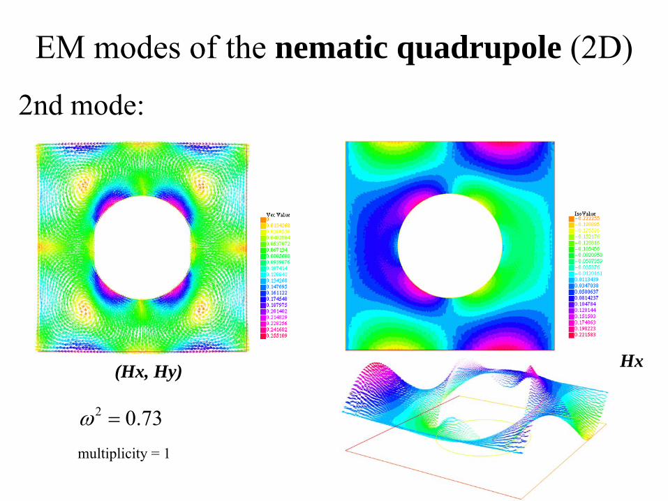
EM modes of the nematic quadrupole (2D)

(Hx, Hy)

2nd mode:

Hx

73.02 multiplicity = 1

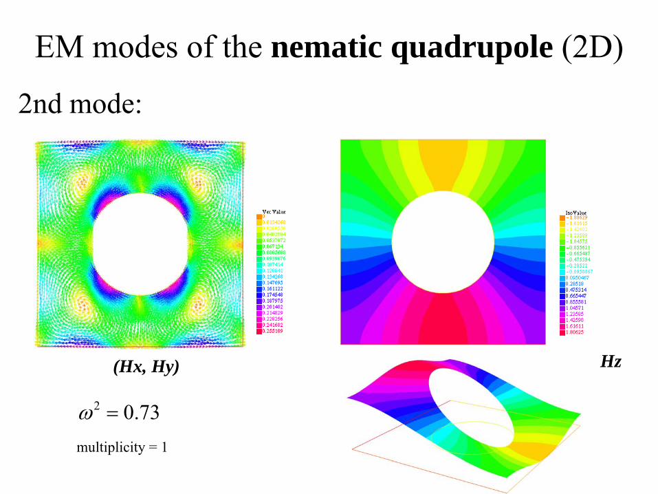
EM modes of the nematic quadrupole (2D)

(Hx, Hy)

2nd mode:

Hz

73.02 multiplicity = 1

EM modes of the nematic quadrupole (2D)

(Hx, Hy)

3rd mode:

Hx

79.12 multiplicity = 1

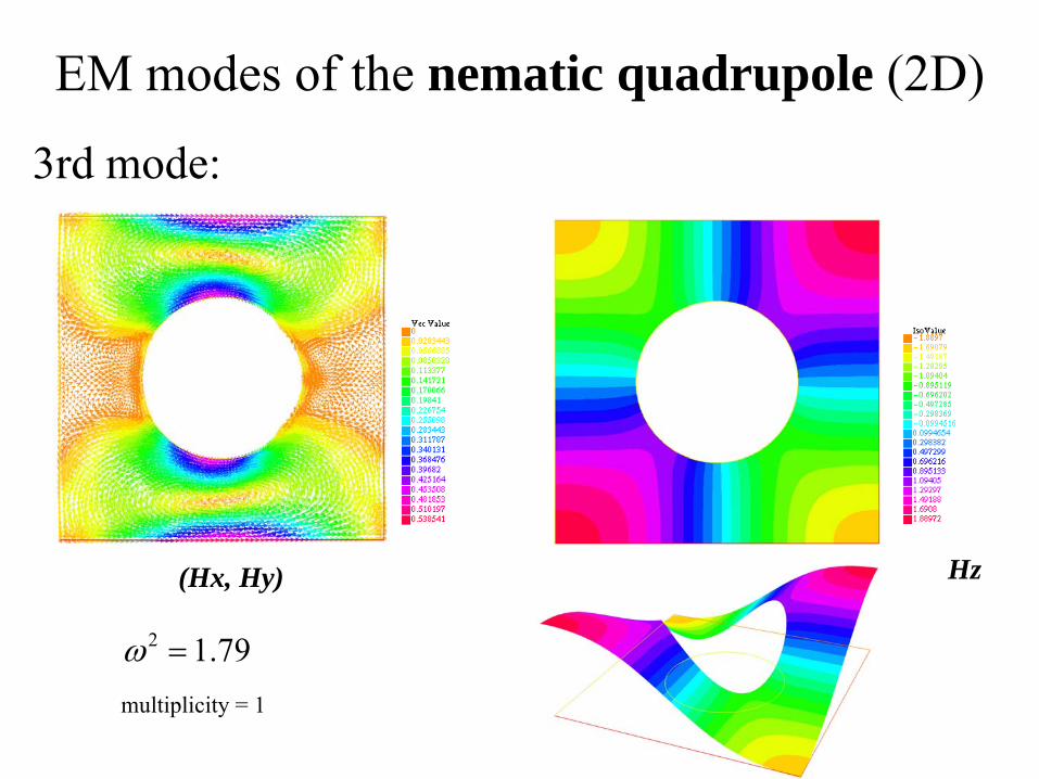
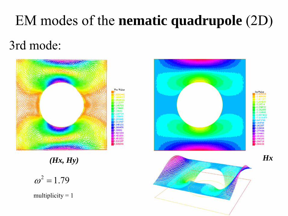
EM modes of the nematic quadrupole (2D)

(Hx, Hy)

3rd mode:

Hz

79.12 multiplicity = 1

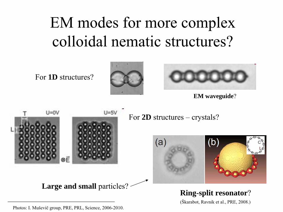
For 1D structures?

EM modes for more complex colloidal nematic structures?

Photos: I. Muševič

group, PRE, PRL, Science, 2006-2010.

EM waveguide?

For 2D structures –

crystals?

(Škarabot, Ravnik et al., PRE, 2008.)

Large and small particles?Ring-split resonator?

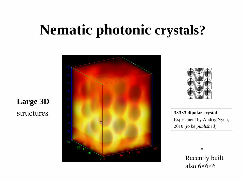
3×3×3 dipolar crystal.Experiment by Andriy Nych,2010 (to be published).

Large 3Dstructures

Nematic photonic crystals?

Recently built also 6×6×6

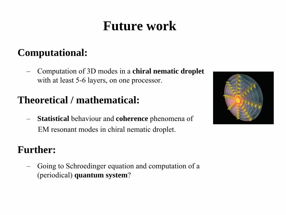
Future work

–

Computation of 3D modes in a chiral nematic droplet with at least 5-6 layers, on one processor.

Computational:

Theoretical / mathematical:

–

Statistical behaviour and coherence phenomena of EM resonant modes in chiral nematic droplet.

–

Going to Schroedinger equation and computation of a (periodical) quantum system?

Further: