Embed Size (px)
Citation preview
PHOTONIC-ENABLED BROADBAND RADIO FREQUENCY TECHNIQUES –
ARBITRARY WAVEFORM GENERATION, RANGING AND WIRELESS
COMMUNICATION
A Dissertation
Submitted to the Faculty
of
Purdue University
by
Yihan Li
In Partial Fulfillment of the
Requirements for the Degree
of
Doctor of Philosophy
December 2015
Purdue University
West Lafayette, Indiana

ii
To my family
iii
ACKNOWLEDGMENTS
I would like to thank Professor Andrew M. Weiner for his instruction, guidance and
patience throughout my graduate study. I also would like to express my gratitude to Dr.
Daniel E. Leaird for his invaluable technical support. I would like to thank Prof.
Vladimir M. Shalaev, Prof. James S. Lehnert, Prof. Mark R. Bell and Prof. Daniel S.
Elliott for serving as my Ph.D. committee members and for their helpful comments and
guidance throughout.
I would like to thank my current and former colleagues in the Ultrafast Optics and
Optical Fiber Communications Laboratory, Dr. Victor Torres-Company, Dr. Xiaoxiao
Xue, Dr. Joseph Lukens, Dr. Hyoung-Jun Kim, Dr. Jian Wang, Dr. Dennis Lee, Mr. A.J.
Metcalf, Mr. Amir Rashidinejad, Mr. Yang Liu, Mr. Bohao Liu and others for valuable
discussions. I would like to thank all the staff of Purdue University who have provided a
warm environment and made being an international student a great experience. Finally, I
would like to thank my family for their love and support.
iv
TABLE OF CONTENTS
Page
LIST OF TABLES ............................................................................................................. vi
LIST OF FIGURES .......................................................................................................... vii
ABSTRACT ..................................................................................................................... xiii
1. INTRODUCTION .......................................................................................................... 1
2. PHOTONIC GENERATION OF BROADBAND ARBITRARY RADIO
FREQUENCY WAVEFORMS ..................................................................................... 6
2.1. Background ............................................................................................................... 6
2.2. Optical Pulse Shaping and Frequency-to-Time Mapping ........................................ 7
2.3. Amplitude-Mismatched Pseudorandom Sequence Modulation ............................. 11
2.3.1. Theory .............................................................................................................. 12
2.3.2. Experimental Configuration ............................................................................. 17
2.3.3. Experimental Results ....................................................................................... 20
2.4. Dual-Shaper Photonic RF-AWG ............................................................................ 27
2.4.1. Experimental Configuration ............................................................................. 27
2.4.2. Experimental Validation .................................................................................. 28
2.5. Phase-Shifted Pseudorandom Sequence Modulation ............................................. 34
2.6. Arbitrary Waveform Generation in W-band .......................................................... 41
2.6.1. Experimental Configuration ............................................................................. 42
2.6.2. Experimental Results ....................................................................................... 43
2.7. Summary ................................................................................................................. 47
3. HIGH RESOLUTION UNAMBIGUOUS RANGING ................................................ 49
3.1. Background ............................................................................................................. 49
3.2. Ultra-wideband Unambiguous Ranging ................................................................. 51
3.3. Ultra-fine Resolution Unambiguous Ranging in W-band ...................................... 55
3.4. Summary ................................................................................................................. 61
4. ULTRA WIDEBAND WIRELESS COMMUNICATION .......................................... 62
4.1. Background ............................................................................................................. 62
4.2. Spread Spectrum Channel Sounding ...................................................................... 65
4.3. Pre-compensation and Data Modulation ................................................................ 70
4.4. Data Transmission .................................................................................................. 73
4.5. Phase Compensation vs. Time Reversal ................................................................. 79

v
Page
4.6. Summary ................................................................................................................. 83
5. REVIEW AND FUTURE RESEARCH DIRECTIONS .............................................. 84
5.1. Review .................................................................................................................... 84
5.2. Future Research Directions .................................................................................... 85
LIST OF REFERENCES .................................................................................................. 87
VITA ................................................................................................................................. 93

vi
LIST OF TABLES
Table Page
3.1 Comparision of prominent MMW and sub-THz ranging system ............................... 62
vii
LIST OF FIGURES
Figure Page
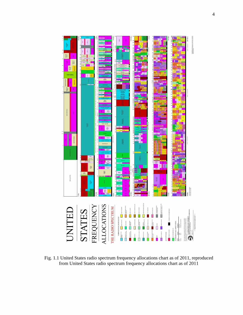
1.1 United States radio spectrum frequency allocations chart as of 2011 ...........................4
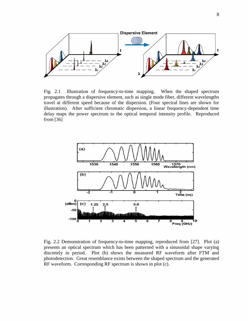
2.1 Illustration of frequency-to-time mapping. When the shaped spectrum propagates
through a dispersive element, such as single mode fiber, different wavelengths
travel at different speed because of the dispersion. (Four spectral lines are shown
for illustration). After sufficient chromatic dispersion, a linear frequency-
dependent time delay maps the power spectrum to the optical temporal intensity
profile. .........................................................................................................................8
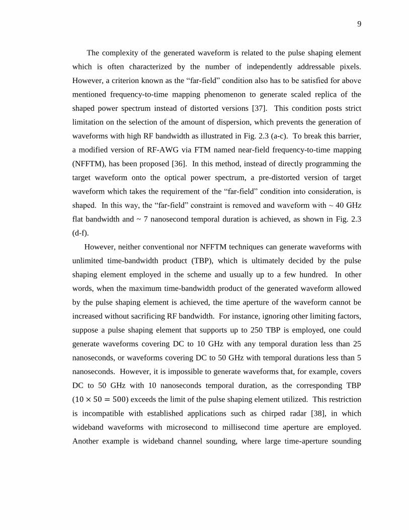
2.2 Demonstration of frequency-to-time mapping. Plot (a) presents an optical
spectrum which has been patterned with a sinusoidal shape varying discretely in
period. Plot (b) shows the measured RF waveform after FTM and photodetection.
Great resemblance exists between the shaped spectrum and the generated RF
waveform. Corresponding RF spectrum is shown in plot (c). .....................................8
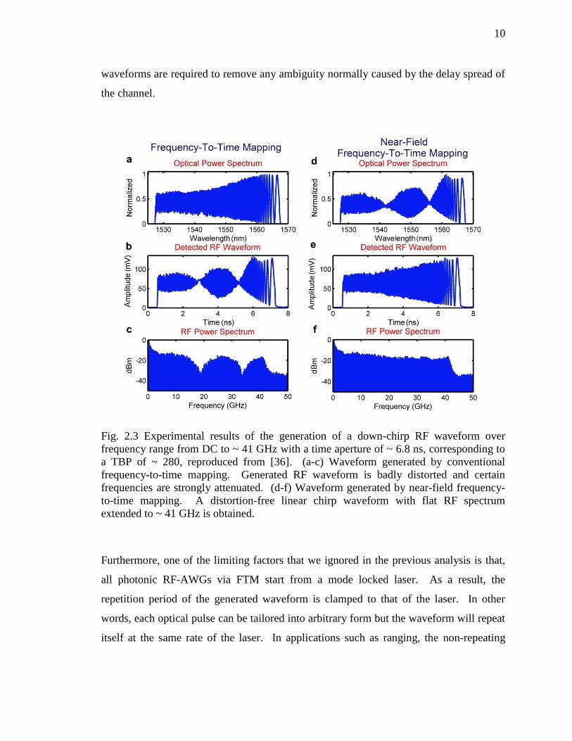
2.3 Experimental results of the generation of a down-chirp RF waveform over
frequency range from DC to ~ 41 GHz with a time aperture of ~ 6.8 ns,
corresponding to a TBP of ~ 280. (a-c) Waveform generated by conventional
frequency-to-time mapping. Generated RF waveform is badly distorted and
certain frequencies are strongly attenuated. (d-f) Waveform generated by near-
field frequency-to-time mapping. A distortion-free linear chirp waveform with
flat RF spectrum extended to ~ 41 GHz is obtained .................................................. 10
2.4 Illustration of a repetitive chirped waveform with period T and a full duty cycle.
Autocorrelation with compressed peaks repeating exactly every T plotted the in
bottom figure. ............................................................................................................. 13
2.5 Illustration of a length-L pn sequence modulated onto a period-T linear chirped
waveform. Top: the polarity of each basis waveform is determined by the
sequence labeled on top. The PN sequence has a period of L. Bottom:
corresponding autocorrelation function. Strong peaks are separated T∙L away
from each other, with all other previously 4-ns separated peaks attenuated and
flipped ........................................................................................................................ 13
viii
Figure Page
2.6 Illustration of an amplitude mismatched PN sequence of length L modulated onto a
period T chirp waveform train. Top: Relative amplitude of all 1s in the sequence
is adjusted to 1+p, where p =2
√L+1. Bottom: corresponding autocorrelation
function. Now the function has only T∙L separated peaks, all the T-separated
weak peaks as in Fig. 2.5 are fully suppressed .......................................................... 15
2.7 Schematic of experimental setup. ML Laser: mode-locked laser. IM: intensity
modulator. PD: photodetector. .................................................................................. 19
2.8 Detailed setup of the dispersion block, indicated by the red dash rectangle in Fig.
2.7. A pair of circulators is connected by a spool of dispersive fiber. Such scheme
ensures the optical signals in both arms propagating through the same piece of
fiber. ........................................................................................................................... 19
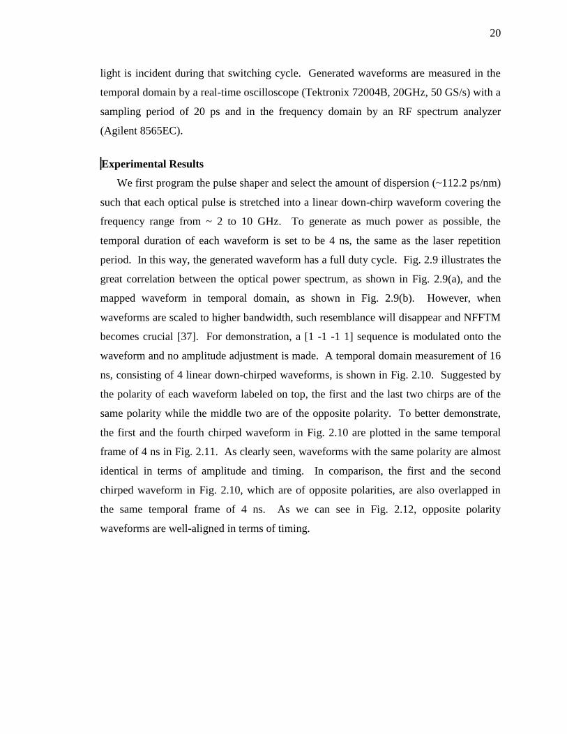
2.9 Demonstration of frequency-to-time mapping. (a) Optical spectrum shaped with a
linear period-increased sinusoidal amplitude modulation. (b) Corresponding RF
waveform after propagation through dispersion and optical-to-electrical
conversion. ................................................................................................................. 21
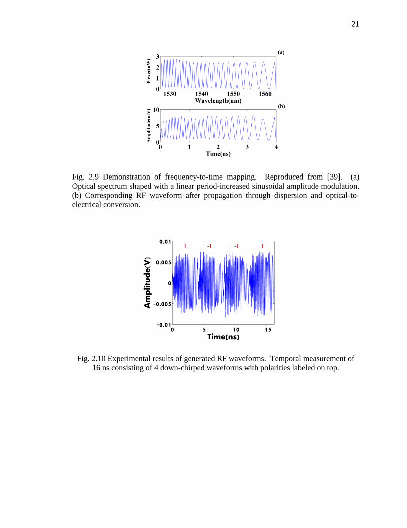
2.10 Experimental results of generated RF waveforms. Temporal measurement of 16
ns consisting of 4 down-chirped waveforms with polarities labeled on top. ............. 21
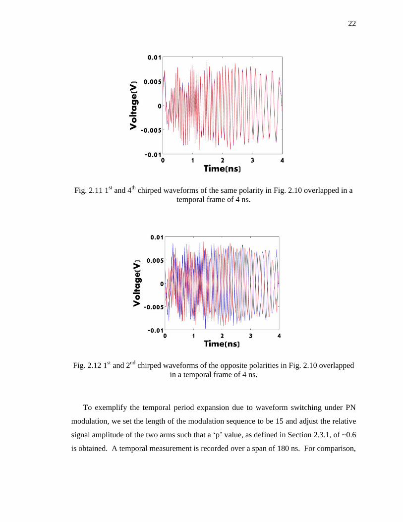
2.11 1st and 4th chirped waveforms of the same polarity in Fig. 2.10 overlapped in a
temporal frame of 4 ns ............................................................................................... 22
2.12 1st and 2nd chirped waveforms of the opposite polarities in Fig. 2.10 overlapped
in a temporal frame of 4 ns ........................................................................................ 22
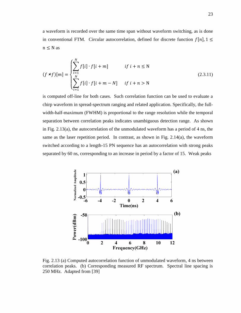
2.13 (a) Computed autocorrelation function of unmodulated waveform, 4 ns between
correlation peaks. (b) Corresponding measured RF spectrum. Spectral line
spacing is 250 MHz. ................................................................................................... 23
2.14 (a) Computed autocorrelation function of the waveform modulated by a length 15
amplitude mismatched PN sequence. 60 ns between correlation peaks. (b)
Magnified view of the sidelobe from 22 to 30 ns in (a), extinction raito ~ 19 dB.
(c) Corresponding measured RF spectrum, similar envelope as in Fig. 2.13(b), but
with a much closer spaced spectral line (measured to be 16.67 MHz, not shown
here). ......................................................................................................................... 24
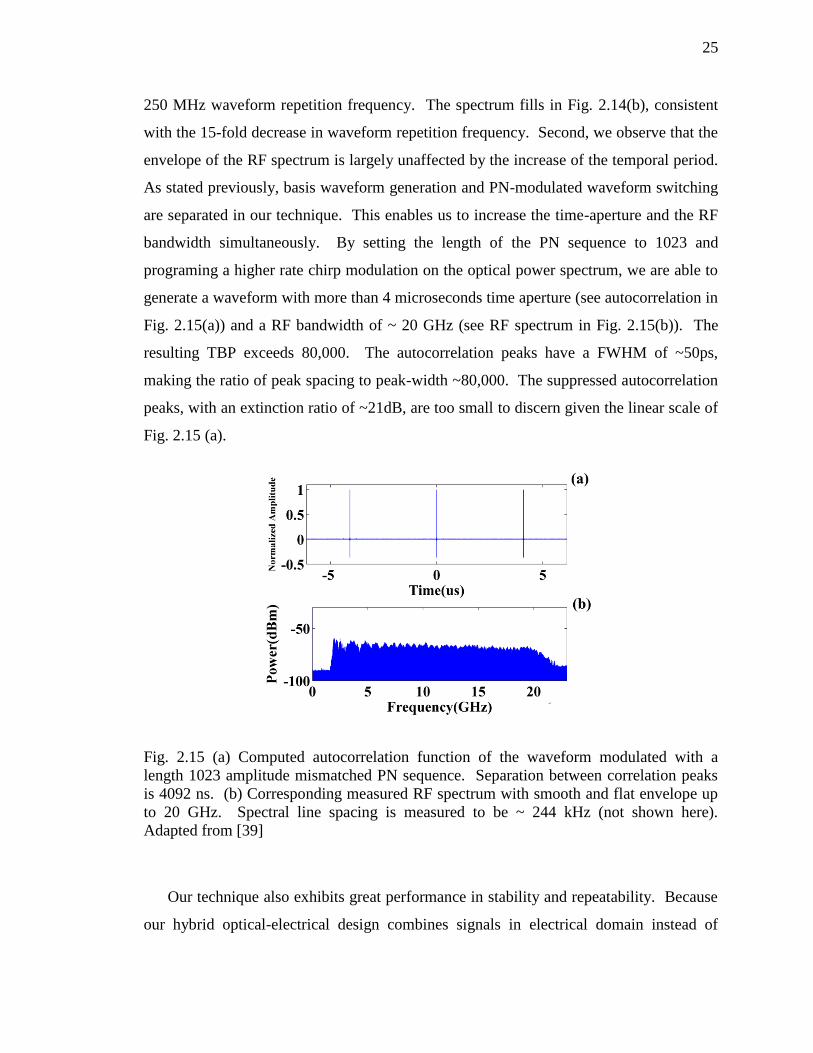
2.15 (a) Computed autocorrelation function of the waveform modulated with a length
1023 amplitude mismatched PN sequence. Separation between correlation peaks
is 4092 ns. (b) Corresponding measured RF spectrum with smooth and flat
envelope up to 20 GHz. Spectral line spacing is measured to be ~ 244 kHz (not
shown here). ............................................................................................................... 25
ix
Figure Page
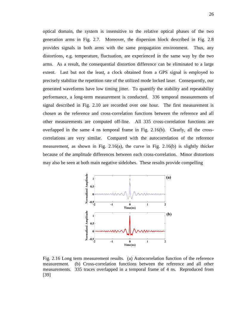
2.16 Long term measurement results. (a) Autocorrelation function of the reference
measurement. (b) Cross-correlation functions between the reference and all other
measurements. 335 traces overlapped in a temporal frame of 4 ns. ......................... 26
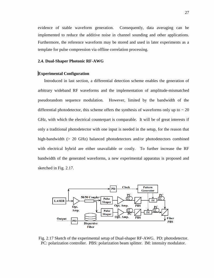
2.17 Sketch of the experimental setup of Dual-shaper RF-AWG. PD: photodetector.
PC: polarization controller. PBS: polarization beam splitter. IM: intensity
modulator ................................................................................................................... 27
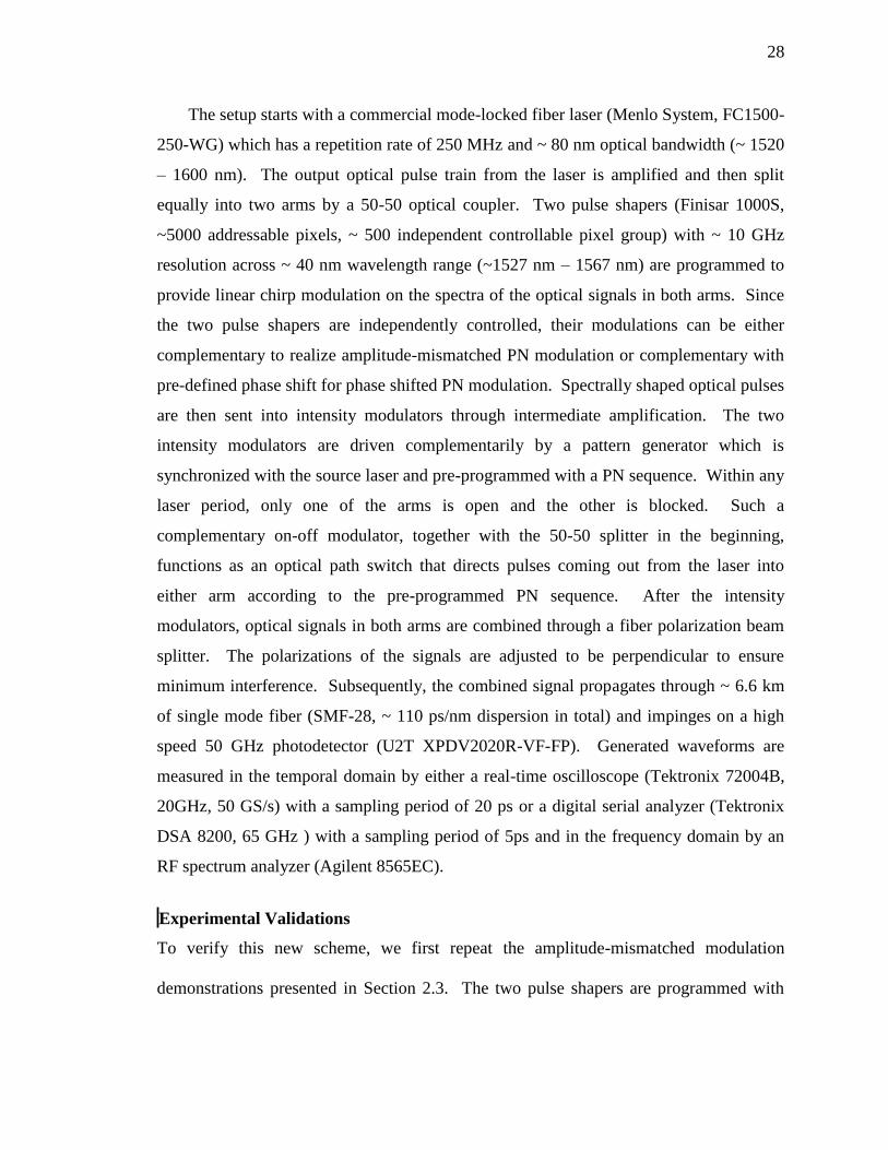
2.18 Experimental measurement of linear chirped waveform modulated with
amplitude mismatched PN sequence. Five basis waveforms in a span of 20 ns ....... 30
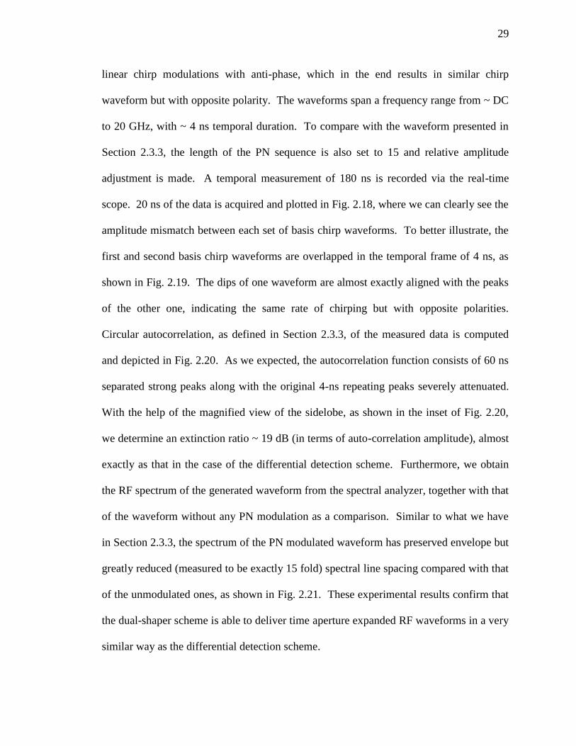
2.19 1st and 2nd basis linear chirped waveforms in Fig. 2.18 overlapped in a temporal
frame of 4 ns. Dips from one waveform are aligned with corresponding peaks of
the other, indicating the same chirping profile but opposite polarity ........................ 30
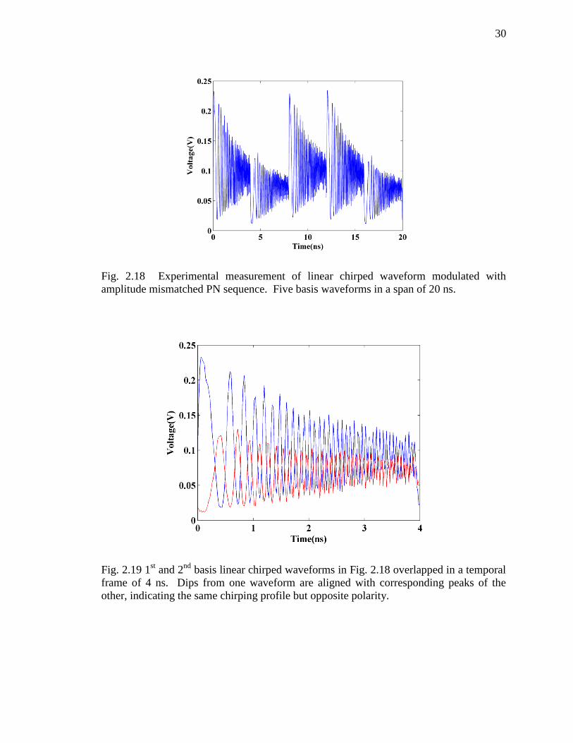
2.20 Computed autocorrelation function of a 180 ns measurement of a linear chirped
waveform modulated with a length-15 amplitude mismatched PN sequence. 60 ns
between correlation peaks. Inset: magnified view of the sidelobe level from 22 to
30 ns. Extinction ratio ~ 19 dB ................................................................................. 31
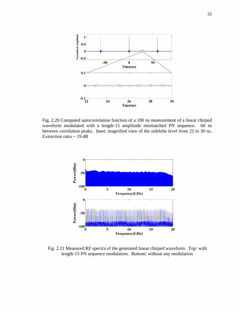
2.21 Measured RF spectra of the generated linear chirped waveform. Top: with
length-15 PN sequence modulation. Bottom: without any modulation .................... 31
2.22 Measured RF spectrum of a ~ DC- 40 GHz linear chirped waveform modulated
with a length 15 amplitude mismatched PN sequence. Spectral line spacing is
measured to be 16.67 MHz, corresponding to a TBP ~ 2400 .................................... 32
2.23 Long term repeatability measurement of waveform described in Fig. 2.18. Red
curve: autocorrelation of the reference measurement. Blue curves: cross-
correlations between the reference and other 59 measurements ................................ 33
2.24 Measurement of frequency hopping waveform whose instantaneous frequency
resembles Purdue logo ............................................................................................... 34
2.25 A Logo of Purdue University .................................................................................... 34
2.26 Two basis waveforms modulated with a ~ 29 degree phase shifted PN sequence
overlapped in a temporal frame of 4 ns. Unlike Fig. 2.19, no amplitude
mismatching but the dips of one basis waveform are not aligned with the peaks of
the other. ..................................................................................................................... 37
2.27 Computed autocorrelation of a measurement of 180 ns of the waveforms in Fig.
2.26. 60 ns between correlation peaks. Inset: magnified view of the sidelobe level
from 22 to 30 ns. ........................................................................................................ 38
x
Figure Page
2.28 Experimental measurements of photonically generated linear chirped waveforms
with different modulation schemes. Top: no modulation. Mid: with amplitude-
mismatched PN sequence modulation. Bottom: with phase-shifted PN sequence
modulation.. ................................................................................................................ 39
2.29 Overlapped basis waveforms for photonically generated linear chirped
waveforms with different modulation schemes. Top: no modulation. Mid: with
amplitude-mismatched PN sequence modulation. Bottom: with phase-shifted PN
sequence modulation. ................................................................................................. 40
2.30 Measured RF spectra for photonically generated linear chirped waveforms with
different modulation schemes. Top: DC to 35 GHz. Bottom: Magnification at 20
GHz with 1 GHz span. Blue: no modulation. Green: phase-shifted PN sequence
modulation. Red: amplitude-mismatched PN sequence modulation ........................ 40
2.31 W-band experimental setup. (a) Schematic of waveform generation, transmission
and measurement. NBUTC-PD: near-ballistic uni-travelling-carrier photodetector.
Tx: transmitter antenna. Rx: receiver antenna. LNA: low noise amplifier. (b)
Close-up of optical-to-electrical conversion block, followed by Tx feed. (c)
Transmitter block. (d) Receiver block ...................................................................... 43
2.32 Experimental results of W-band waveform generation though RF-AWG based on
FTM. (a) Measured down-converted waveform with ~ 15 GHz bandwidth. (b)
Retrieved waveform after up-conversion. Frequency ranges from ~ 80 GHz to ~
100 GHz. .................................................................................................................... 44
2.33 Measurement of repetition period expanded W-band RF waveforms. (a) 60 ns
measurement of down-converted W-band chirped waveform train without PN
modulation. (b) 60 ns measurement of down-converted W-band chirped
waveform train with length-15 PN modulation (basis waveforms in red indicating
flipped polarity). ......................................................................................................... 45
2.34 Computed autocorrelations of W-band RF waveforms with different modulation
schemes. (a) Autocorrelation of unmodulated waveforms. (b) Autocorrelation of
length-15 PN modulated waveforms. (c) Autocorrelation of length-1023 PN
modulated waveforms ................................................................................................ 46
2.35 Cross-correlations between a reference chirped waveform and 4000 consecutive
linear down-chirp waveforms (in blue) and autocorrelation of the reference down-
chirp waveform (in red). ............................................................................................ 47
3.1 Sketch of the ambiguity issue in ranging experiment. ............................................... 51
3.2 Sketch of the setup of the one-dimensional ranging experiment. Conducted in the
hallway of the subbasement of MSEE building at Purdue University ....................... 52
xi
Figure Page
3.3 Sketches of the transmitted waveform in the ranging experiment. (a) Regular
repeating linear chirp waveform. (b) Repetition period increased linear chirp
waveform. (c) PN modulated linear chirp waveform ................................................ 53
3.4 Cross-correlations obtained by transmitting 3 different waveforms sketched in Fig.
4.2. Normalized to 3.2 V2∙ps. (a): Unmodulated chirps as in Fig. 4.2(a) are
transmitted, 4 ns between peaks of P1, 4 ns between peaks of P2. Horizontal
magnification from 2 to 10 ns is shown on right. (b): Repetition period increased
chirps as in Fig. 4.2 (b) are transmitted. ~ 4.04 ns between peaks of P1 and P2.
Peaks are attenuated by a factor of ~ 15 compared with those in (a). Magnification
from 2 to 10 ns horizontally and -0.1 to 0.1 vertically is shown on right. (c):
Length-15 PN modulated chirps as in Fig. 4.2(c) are transmitted. ~4.04 ns
between peaks of P1 and P2, corresponding to ~ 1.2 m assuming a propagation
speed of light. Horizontal magnification from 2 to 10 ns is shown on right ............. 54
3.5 Setup schematic for ultra-high resolution W-band ranging experiments. Ball A has
a radius of 4 cm. Flat sheets B1 and B2 are 10×10 cm. Flat sheet C is 10×15 cm. . 56
3.6 Photograph of the experimental setup of the ultra-high resolution W-band ranging
experiments ................................................................................................................ 56
3.7 Unambiguous W-band ranging results. (a) Long range W-band detection with
unmodulated sensing waveforms. (b) Long range W-band detection with length-
15 PN-modulated sensing waveforms. (c) Magnified view from 24-26 ns of (b).
(d) Achieved finest range resolution (single measurement). ..................................... 58
3.8 Ultra-high resolution W-band ranging experiment results. (a-c) with ~ 10mm, ~
6mm and ~ 4mm target separation, respectively (multiple measurements) ............... 59
4.1 Sketch of the signal distortion introduced by multipath. Received signal changes
dramatically with even a few decimeters of receiver location. .................................. 64
4.2 Environmental layout of the transmitter and receiver in line-of-sight and non-line-
of-sight geometry. ...................................................................................................... 68
4.3 Calculated wireless channel information (line-of-sight). (a) Impulse response. 7.5
ns between red lines (b) Frequency response ............................................................. 69
4.4 Calculated wireless channel information (non-line-of-sight). (a) Impulse
response. RMS delay spread ~ 17.1 ns. Inset: Magnification of the first 8 ns of
the impulse response. (b) Frequency response from 2-18 GHz. ............................... 70
4.5 Block diagram of the ultra-wideband wireless communication system apparatus.
ML: mode-locked laser. PD: photodetector. Amp: amplifier. ................................. 72
xii
Figure Page
4.6 Received signals with BPSK data modulation (line-of-sight). (a) With 7.5 ns pre-
distorted waveform as input. Red dots indicate the sampling position for BER
calculation. (b) With short pulse inputs .................................................................... 75
4.7 Eye diagram of the received signal corresponding to the situation of Fig. 4.6(a). .. 75
4.8 Four bit periods of the received signal with OOK data modulation (non-line-of-
sight). (a) With short pulses as input. Inset: eye diagram consisting of 127
overlapped traces, with 0.6 ns horizontal span. (b) With phase-compensated
waveform as input. FWHM of each compressed pulse ~ 48 ps. Green dash line
indicates threshold that determines 1/0. The 4 bits are decoded as 1, 0, 1, 0. Inset:
eye diagram consisting of 127 overlapped traces, with 0.6 ns horizontal span. ........ 76
4.9 Received signals with BPSK modulation (non-line-of-sight). (a) Ten bit periods
of the received signal with BPSK data modulation, 7.5 ns phase-compensated
waveform as input. FWHM of each compressed pulse ~ 48 ps. (b) Blue: two bit
period of the received signal. Red: simulated received signal generated by
convolving target compensation waveform with the impulse response offline ......... 78
4.10 Eye diagram of BPSK data modulated received signal (NLOS). 4000 overlapped
bit periods. Inset: Horizontal magnification from -0.2 to 0.2 ns. .............................. 78
4.11 Distributions of the received positive peak voltage, normalized to the average
positive peak voltage. (a) Simulation, computed based on the target pre-
compensation waveform, measured impulse response, and received SNR of 22 dB.
Red: Gaussian fit. (b) Experimental result. Red: Gaussian fit. ................................. 79
4.12 Eye diagrams of received signals. (a) Phase compensated waveforms as input.
(b) Time reversed waveforms as input ....................................................................... 80
4.13 Distributions of the received positive peak voltage. (a) Phase compensated
waveforms as input. Red: Gaussian fit. (b) Time reversed waveforms as input.
Red: Gaussian fit ........................................................................................................ 81
4.14 Bit error rate against received signal to noise ratio. Blue: Phase compensation.
Red: Time reversal ..................................................................................................... 82
4.15 Experimental demonstration of image transmission. (a) Original image. (b)
Reconstructed image when phase compensation is used, measured SNR ~ 15 dB.
(c) Reconstructed image when time reversal is used, measured SNR ~ 17.2 dB. ..... 83
xiii
ABSTRACT
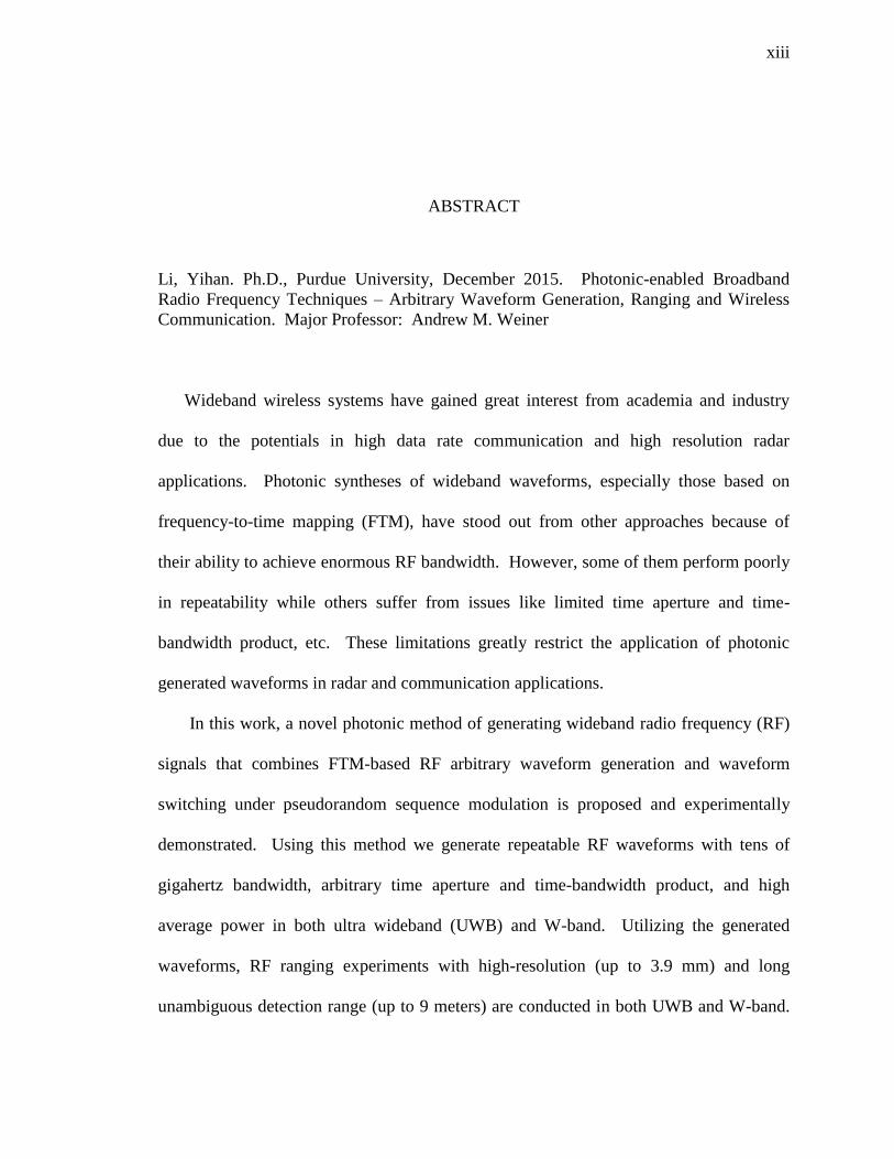
Li, Yihan. Ph.D., Purdue University, December 2015. Photonic-enabled Broadband
Radio Frequency Techniques – Arbitrary Waveform Generation, Ranging and Wireless
Communication. Major Professor: Andrew M. Weiner
Wideband wireless systems have gained great interest from academia and industry
due to the potentials in high data rate communication and high resolution radar
applications. Photonic syntheses of wideband waveforms, especially those based on
frequency-to-time mapping (FTM), have stood out from other approaches because of
their ability to achieve enormous RF bandwidth. However, some of them perform poorly
in repeatability while others suffer from issues like limited time aperture and time-
bandwidth product, etc. These limitations greatly restrict the application of photonic
generated waveforms in radar and communication applications.
In this work, a novel photonic method of generating wideband radio frequency (RF)
signals that combines FTM-based RF arbitrary waveform generation and waveform
switching under pseudorandom sequence modulation is proposed and experimentally
demonstrated. Using this method we generate repeatable RF waveforms with tens of
gigahertz bandwidth, arbitrary time aperture and time-bandwidth product, and high
average power in both ultra wideband (UWB) and W-band. Utilizing the generated
waveforms, RF ranging experiments with high-resolution (up to 3.9 mm) and long
unambiguous detection range (up to 9 meters) are conducted in both UWB and W-band.
xiv
Furthermore, based on our photonic RF-AWG, a communication system is assembled to
realize fast channel sounding, pre-compensated signal generation and real-time wireless
data transmission in the UWB. Error-free data transmissions covering 2 – 18 GHz at 250
Mbits/sec in OOK and BPSK modulation formats are realized in both highly dispersive
line-of-sight (LOS) and dense-multipath non-line-of-sight (NLOS) environments. Our
experiments are the first to our knowledge to directly compare the communication
performance of phase compensation and time reversal schemes in a strong multipath
channel; our results demonstrate that the phase compensation scheme provides
significantly enhanced suppression of intersymbol interference.
1
1. INTRODUCTION
In recent decades we have witnessed tremendous advancement in radio frequency
(RF) technology, impacting applications such as radar and high-speed data transmission.
This rapid progress in RF techniques has resulted in a more and more congested
spectrum. As illustrated in Fig. 1.1, lower frequency bands have been fully allocated to
various purposes. Motivated by the hunger for more capacity, researchers have been
trying to circumvent the crowed lower RF frequency bands by searching for possibilities
to explore undeveloped higher frequency bands. In addition, physical law governs that
the capacity of a radio frequency system is inversely proportional to the utilized
bandwidth. Consequently, radio frequency systems with high center frequency and
broad bandwidth have drawn the attentions from both academia and industry. Ultra
wideband (UWB) and W-band are examples of suitable candidates.
The study of modern ultra wideband technology started more than three decades ago
[1]. In the year of 2002, the Federal Communications Commission (FCC) allocated a 7.5
GHz RF bandwidth from 3.1 to 10.6 GHz for unlicensed use in data communication,
radar, and safety applications. Such enormous frequency bandwidth provides the UWB
system with several unique advantages over the conventional narrow band systems:
High Data Rate: This is one of the direct consequences of having a large RF
bandwidth, as the data rate of a communication system is generally proportional to its RF
bandwidth [2]. The data rate that can be offered by UWB system cannot possibly be
achieved by conventional narrow band systems [3].
High timing resolution: This is one consequence of the large RF bandwidth
viewing from temporal domain aspect. The achievable temporal domain pulses are
extremely narrow compared with those from narrow band system, leading to the
2
possibility of a much better timing precision than global positioning system (GPS) and
other radio systems. Such property could facilitate applications such as locating and
tracking.
Noise-like signal spectrum: As regulated by FCC, the power spectral density
emission limit of UWB transmitters is -41.3 dBm/MHz. Such low energy density and
pseudorandom characteristics make the transmitted UWB signal less likely to be detected
by unintended users and to interfere significantly with other existing narrow band radio
systems.
Low complexity and reduced cost: In contrast to conventional systems where
baseband signals are up-converted before transmission, in UWB systems, transmitters
directly produce waveforms that do not require an extra mixing stage. This could
potentially reduce the complexity in designing and fabrication of UWB systems.
The above mentioned advantages portray a promising vista of a new generation of
wireless communications and other applications, e.g. wireless personal area network
(WPAN) of short distance, high data rate communication.
The W-band of the microwave portion of the electromagnetic spectrum ranges from
75 to 110 GHz, corresponding to a range of wavelength from ~2.7 to 4 mm. This band
has already been used for satellite communications, millimeter-wave radar research,
military radar targeting and tracking applications, and some non-military applications.
Compared with radar systems in other bands with lower frequency, W-band offers a
higher spatial resolution with a reduced antenna size [4]. In terms of communications
capability, W band provides high data rates when employed at high altitudes and in
space. As shown in Fig. 1.1, the 71–76 GHz and 81–86 GHz segment of the W band is
allocated by the International Telecommunication Union to satellite services. In addition,
W-band waveforms are transparent with respect to plywood, plasterboard, ceramics,
paper, windows and clothes, while remaining highly reflective for dangerous metallic
weapons and living objects with high water content [5]. As a result, W-band waveforms
have the potential to become a powerful tool for concealed object detection. W-band also
provides access to ultrabroad bandwidth for applications like ultrahigh-speed wireless
3
communication [6-11], high-resolution ranging [4, 12, 13], electromagnetic imaging and
tomography [14-17], and high-speed spectroscopy [18-21].
A common obstacle that prevents the exploration of the aforementioned two
frequency bands is the shortage of arbitrary waveforms synthesis with broad bandwidth,
high fidelity, and low timing jitter. Without appropriate waveform generation, it’s
extremely challenging to fully utilize the potential of these broad frequency bands. This
issue has motived us to search for solutions through both theoretical and experimental
studies. The rest of this paper is organized as follows: In Chapter 2, comparison between
electrical and photonic approaches to generating arbitrary RF waveforms are presented to
highlight the advantages of utilizing optical techniques. After the brief introduction of
optical pulse shaping and frequency-to-time mapping, a novel photonic technique named
amplitude-mismatched pseudorandom sequence modulation is mathematically
investigated and experimentally demonstrated. Using this technique, broadband RF
waveforms are synthesized and the limitation of fixed repetition period in conventional
photonic radio frequency arbitrary waveform generation (RF-AWG) is overcome. The
generated waveforms have up to 40 GHz RF bandwidth, with repetition period arbitrarily
adjustable. The time-bandwidth product reaches as high as over 80000, and the long-
term repeatability is experimentally proven to be superb. Subsequently, a modified
experimental apparatus is proposed to scale the generated waveforms up to W-band,
resulting in the synthesis of arbitrary waveforms covering ~ 75-100 GHz. To our
knowledge, this is the first demonstration of RF-AWG in W-band. In addition, the same
experimental setup is used to implement another proposed modulation technique --
phase-shifted pseudorandom sequence modulation, which delivers the maximum average
power in the peak-voltage-limited scenario.
To demonstrate one of the applications of the generated wideband RF waveforms, a
one-dimensional ranging experiment is introduced at the beginning of Chapter 3.
Problems experienced by conventional photonic-assisted ranging systems are discussed,
followed by experimental results presenting significant improvement using the photonic
RF waveform generation scheme described in Chapter 2. Next, the setup is up-scaled to
4
Fig. 1.1 United States radio spectrum frequency allocations chart as of 2011, reproduced
from United States radio spectrum frequency allocations chart as of 2011
5
W-band, enabling multiple-object localization with ultra-fine resolution and
unambiguous detection. A record 3.9 mm spatial resolution and over 9 meters
unambiguous range are experimentally achieved.
Chapter 4 focuses on the realization of broadband wireless data transmission over the
“extended” UWB. Taking advantage of the broadband RF waveform generated by our
scheme, channel sounding experiments up to 2-18 GHz are conducted to characterize the
impulse responses of two distinct wireless channels both in temporal and frequency
domains. To overcome the signal distortions of the wireless propagation environment
which are primarily caused by dispersion and multipath, a phase-compensation technique
is implemented to pre-distort the input waveform, enabling self-compression while
propagating through the channel and resulting in short-pulse formation at the receiver.
Error free communications are realized in both line-of-sight and non-line-of-sight channel
geometries, validating the feasibility of high-speed wireless data transmission in highly-
dispersed, dense-multipath indoor environment. Moreover, for the first time to our
knowledge, phase compensation and time reversal are directly compared in data
transmission experiment to confirm a previous prediction made by our group through
simulation that phase compensation delivers significant improvement over time reversal
in terms of the suppression of intersymbol interference.
A review of the proposed techniques and achieved results is made in Chapter 5, with
emphasis on the potential of photonic-assisted broadband RF system as a candidate for
the next generation of wireless communications. Furthermore, future research directions
are also discussed to further increase the capacity of the communications system.
6
2. PHOTONIC GENERATION OF BROADBAND ARBITRARY
RADIO FREQUENCY WAVEFORMS
2.1. Background
It is quite natural to utilize electrical approaches for the generation of arbitrary RF
waveforms. As a matter of fact, commercial electrical arbitrary waveform generators (E-
AWG) have been widely used in broadband RF applications. Owing to the large physical
memory, through digital signal processing (DSP) and digital to analog conversion
(DAC), E-AWG can deliver broadband RF waveforms up to millisecond level. However,
at the time when we started our research, the state-of-the-art E-AWG could only offer RF
bandwidth up to 9.6 GHz. Even with recently advances, the bandwidth of the RF
waveforms generated electrically is still limited to ~ 20 GHz due to the relatively slow
speed of DAC [22]. In addition, severe electromagnetic interference (EMI) and large
timing jitter have long been the compromising factors of E-AWG. Last but not the least,
as the bandwidth of the waveform scales up, the attenuation experienced by the electrical
signal in the coaxial cable during the wired distribution increases drastically. All these
problems motivate researchers to look for alternative solutions.
To this day, various photonic synthesis schemes, typically followed by photodetection
to covert optical signals to electrical ones, have been proposed and experimentally
validated [23-31]. These technologies take advantage of the fact that optical systems are
generally immune to EMI. In addition, optical fibers could be used to transmit optical
signals from base station to access point prior to optical to electrical (O/E) conversion to
significantly reduce the propagation loss during wired distribution, which is the key
philosophy of the emerging radio-over-fiber (RoF) technique [32]. More importantly,
the RF bandwidth of the waveforms generated by photonic techniques can easily surpass
the limit of available electrical counterparts to reach tens, even hundreds of gigahertz.
7
Heterodyne mixing of a fixed frequency combined with a rapidly frequency sweeping
laser [31] can generate RF waveforms with high bandwidth, time apertures up to
microsecond range and potentially fast chirp rates. However, the repeatability and
stability of such system remains in doubt. Another type of technique [28, 29, 33], which
offers a high degree of repeatability, is based on the switching between multiple basis
waveforms obtained via line-by-line pulse shaping of optoelectronically generated
frequency combs [34]. Such a switching scheme allows arbitrarily large time-aperture
without waveform repetition. Yet, limited by the resolution of optical pulse shaper, the
switching is restricted to basis waveforms of low complexity, with only up to a few
hundred picoseconds long time aperture and RF programmable features at 5 GHz level.
2.2. Optical Pulse Shaping and Frequency-to-Time Mapping
Photonic method [26, 27, 30] that employs optical pulse shaping in conjunction with
frequency-to-time mapping has been under the spotlight since its introduction. It offers
extremely stable and repeatable arbitrary waveforms with high RF bandwidth and a few
nanosecond time apertures. This technique starts from a pulsed mode-locked laser with
wide optical power spectrum. Such optical signal travels through a pulse shaping
element (e.g. Fourier transform pulse shaper [35], chirped fiber Bragg grating [30])
where the amplitude and phase of each group of optical spectral component are
programmed independently. When propagating in a dispersive element, such as single
mode fiber, different frequency components travel at different speeds. Eventually after
enough dispersion, the optical intensity of each pulse will be stretched in time to become
a scaled replica of the shape of the optical power spectrum, a phenomenon known as
frequency-to-time mapping (FTM), as illustrated in Fig. 2.1. When a designated
waveform is programmed onto the optical spectrum and transmitted through carefully
calculated dispersion, it could be obtained after sending the optical signal into an optical-
to-electrical conversion component (photodetector). Demonstration of a shaped optical
spectrum and its corresponding converted RF waveform and RF spectrum are depicted in
Figs. 2.2 (a), (b) and (c), respectively.
8
Fig. 2.1 Illustration of frequency-to-time mapping. When the shaped spectrum
propagates through a dispersive element, such as single mode fiber, different wavelengths
travel at different speed because of the dispersion. (Four spectral lines are shown for
illustration). After sufficient chromatic dispersion, a linear frequency-dependent time
delay maps the power spectrum to the optical temporal intensity profile. Reproduced
from [36]
Fig. 2.2 Demonstration of frequency-to-time mapping, reproduced from [27]. Plot (a)
presents an optical spectrum which has been patterned with a sinusoidal shape varying
discretely in period. Plot (b) shows the measured RF waveform after FTM and
photodetection. Great resemblance exists between the shaped spectrum and the generated
RF waveform. Corresponding RF spectrum is shown in plot (c).
9
The complexity of the generated waveform is related to the pulse shaping element
which is often characterized by the number of independently addressable pixels.
However, a criterion known as the “far-field” condition also has to be satisfied for above
mentioned frequency-to-time mapping phenomenon to generate scaled replica of the
shaped power spectrum instead of distorted versions [37]. This condition posts strict
limitation on the selection of the amount of dispersion, which prevents the generation of
waveforms with high RF bandwidth as illustrated in Fig. 2.3 (a-c). To break this barrier,
a modified version of RF-AWG via FTM named near-field frequency-to-time mapping
(NFFTM), has been proposed [36]. In this method, instead of directly programming the
target waveform onto the optical power spectrum, a pre-distorted version of target
waveform which takes the requirement of the “far-field” condition into consideration, is
shaped. In this way, the “far-field” constraint is removed and waveform with ~ 40 GHz
flat bandwidth and ~ 7 nanosecond temporal duration is achieved, as shown in Fig. 2.3
(d-f).
However, neither conventional nor NFFTM techniques can generate waveforms with
unlimited time-bandwidth product (TBP), which is ultimately decided by the pulse
shaping element employed in the scheme and usually up to a few hundred. In other
words, when the maximum time-bandwidth product of the generated waveform allowed
by the pulse shaping element is achieved, the time aperture of the waveform cannot be
increased without sacrificing RF bandwidth. For instance, ignoring other limiting factors,
suppose a pulse shaping element that supports up to 250 TBP is employed, one could
generate waveforms covering DC to 10 GHz with any temporal duration less than 25
nanoseconds, or waveforms covering DC to 50 GHz with temporal durations less than 5
nanoseconds. However, it is impossible to generate waveforms that, for example, covers
DC to 50 GHz with 10 nanoseconds temporal duration, as the corresponding TBP
(10 × 50 = 500) exceeds the limit of the pulse shaping element utilized. This restriction
is incompatible with established applications such as chirped radar [38], in which
wideband waveforms with microsecond to millisecond time aperture are employed.
Another example is wideband channel sounding, where large time-aperture sounding
10
waveforms are required to remove any ambiguity normally caused by the delay spread of
the channel.
Fig. 2.3 Experimental results of the generation of a down-chirp RF waveform over
frequency range from DC to ~ 41 GHz with a time aperture of ~ 6.8 ns, corresponding to
a TBP of ~ 280, reproduced from [36]. (a-c) Waveform generated by conventional
frequency-to-time mapping. Generated RF waveform is badly distorted and certain
frequencies are strongly attenuated. (d-f) Waveform generated by near-field frequency-
to-time mapping. A distortion-free linear chirp waveform with flat RF spectrum
extended to ~ 41 GHz is obtained.
Furthermore, one of the limiting factors that we ignored in the previous analysis is that,
all photonic RF-AWGs via FTM start from a mode locked laser. As a result, the
repetition period of the generated waveform is clamped to that of the laser. In other
words, each optical pulse can be tailored into arbitrary form but the waveform will repeat
itself at the same rate of the laser. In applications such as ranging, the non-repeating
11
period of the transmitted waveform has to exceed the round trip time of the furthest
object in order to ensure detection without ambiguity. A 10-meter detection range
requires the repetition rate of the laser to be at most 15 MHz, which is well below the
normal operation range of mode locked lasers. Even assuming such lasers are available,
the previously mentioned trade-off between RF bandwidth and time aperture prevents the
generation of waveforms with high average power, which is another requirement for most
radar applications. For example, suppose a spatial resolution of 1.5 cm with an
unambiguity detection range of 150 meters are required in one ranging experiment, which
translate into a temporal resolution of 50 ps and unambiguous range of 0.5 microseconds,
respectively. Such criterions demand a probing waveform with at least 20 GHz RF
bandwidth and 1 microsecond repetition period. If we employ the same pulse shaping
element described in the last paragraph, the maximum time aperture of the generated
waveform with 20 GHz bandwidth is only 12.5 nanoseconds, corresponding to a duty
cycle of only 1.25%. Considering the peak-voltage-limited nature of most photonic RF
systems, such small duty cycle will inevitably result in low transmitted power and poor
performance in object localization.
2.3. Amplitude-mismatched Pseudorandom Sequence Modulation
Here, we propose a novel photonic spread spectrum radio-frequency waveform
generation technique that, for the first time, combines frequency-to-time mapping and
waveform switching [39]. In this work, we generate high complexity basis RF
waveforms with wide bandwidth and time aperture of several nanoseconds. As the time
aperture of generated basis waveform is roughly the same as the repetition period of the
employed laser, the average power reaches almost the maximum as duty cycle
approaches 100%. In addition, by switching between positive and negative polarity
versions of a basis waveform under electrical control according to a pseudorandom (PN)
sequence [40], we are able to increase the time aperture arbitrarily by simply increasing
the length of the PN sequence. Since our switching involves polarity-flipping only, the
average power of it is maintained. The waveforms generated are highly repeatable and,
analogous to noise radar technology [41], are characterized both by high RF bandwidth
and substantial energy spread in time. Moreover, as RF bandwidth and repeat-free time
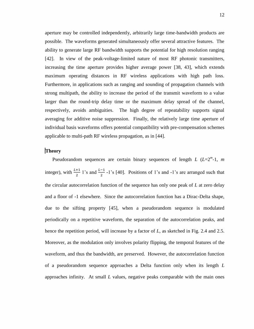
12
aperture may be controlled independently, arbitrarily large time-bandwidth products are
possible. The waveforms generated simultaneously offer several attractive features. The
ability to generate large RF bandwidth supports the potential for high resolution ranging
[42]. In view of the peak-voltage-limited nature of most RF photonic transmitters,
increasing the time aperture provides higher average power [38, 43], which extends
maximum operating distances in RF wireless applications with high path loss.
Furthermore, in applications such as ranging and sounding of propagation channels with
strong multipath, the ability to increase the period of the transmit waveform to a value
larger than the round-trip delay time or the maximum delay spread of the channel,
respectively, avoids ambiguities. The high degree of repeatability supports signal
averaging for additive noise suppression. Finally, the relatively large time aperture of
individual basis waveforms offers potential compatibility with pre-compensation schemes
applicable to multi-path RF wireless propagation, as in [44].
Theory
Pseudorandom sequences are certain binary sequences of length L (L=2m-1, m
integer), with 𝐿+1
2 1’s and
𝐿−1
2 -1’s [40]. Positions of 1’s and -1’s are arranged such that
the circular autocorrelation function of the sequence has only one peak of L at zero delay
and a floor of -1 elsewhere. Since the autocorrelation function has a Dirac-Delta shape,
due to the sifting property [45], when a pseudorandom sequence is modulated
periodically on a repetitive waveform, the separation of the autocorrelation peaks, and
hence the repetition period, will increase by a factor of L, as sketched in Fig. 2.4 and 2.5.
Moreover, as the modulation only involves polarity flipping, the temporal features of the
waveform, and thus the bandwidth, are preserved. However, the autocorrelation function
of a pseudorandom sequence approaches a Delta function only when its length L
approaches infinity. At small L values, negative peaks comparable with the main ones
13
will degrade the performance of the waveform in applications such as multi-object
ranging. Adjustments have to be made to suppress these unwanted peaks.
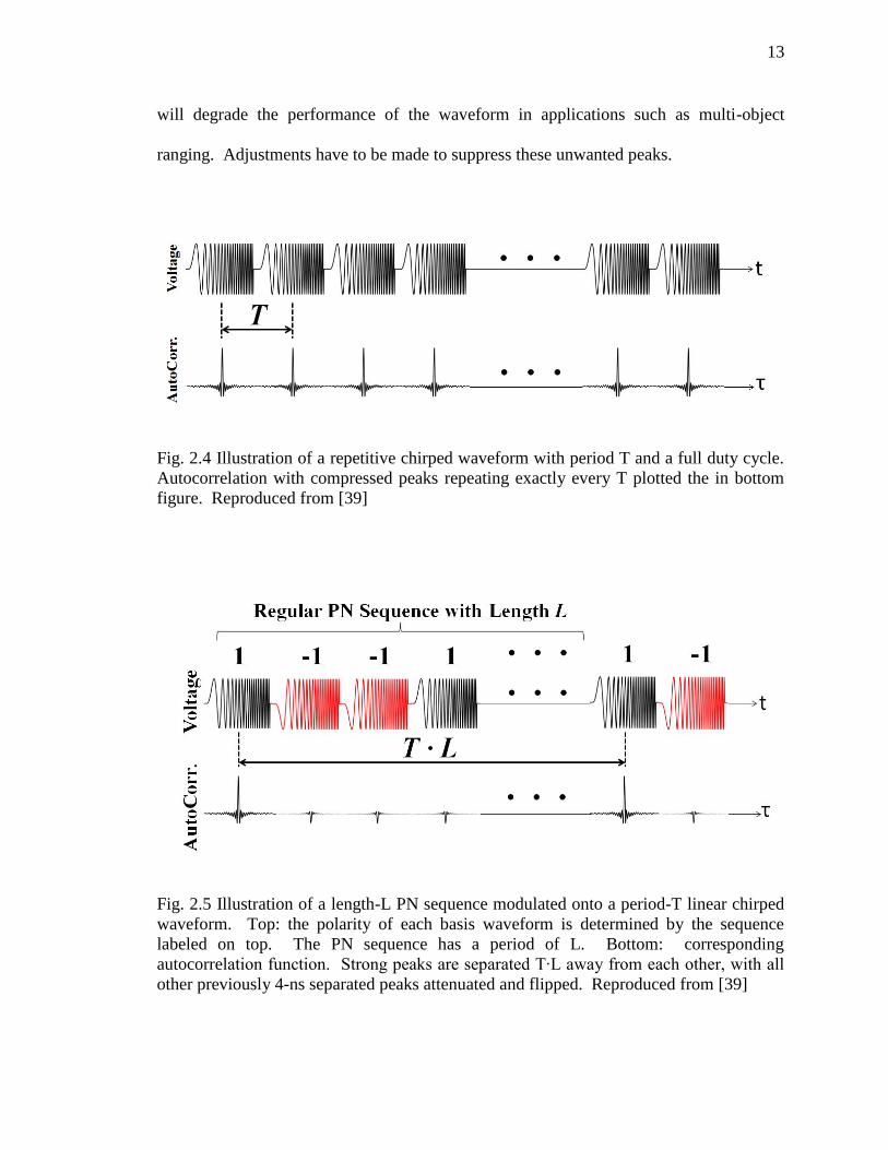
Fig. 2.4 Illustration of a repetitive chirped waveform with period T and a full duty cycle.
Autocorrelation with compressed peaks repeating exactly every T plotted the in bottom
figure. Reproduced from [39]
Fig. 2.5 Illustration of a length-L PN sequence modulated onto a period-T linear chirped
waveform. Top: the polarity of each basis waveform is determined by the sequence
labeled on top. The PN sequence has a period of L. Bottom: corresponding
autocorrelation function. Strong peaks are separated T∙L away from each other, with all
other previously 4-ns separated peaks attenuated and flipped. Reproduced from [39]
14
In Amplitude-mismatched Pseudorandom Sequence Modulation, as illustrated in Fig.
2.6, we adjust all the 1’s in the binary pseudorandom sequence to 1 + 𝑝, where p is a
positive number and keep all the -1’s. The autocorrelation function of such amplitude-
mismatched pseudorandom sequence has non-zero value only at zero delay.
Mathematically, let’s denote a length-L binary pseudorandom sequence by 𝑃𝑁 and define
a length-L unit sequence 𝑈 such that 𝑈[𝑖] = 1 𝑓𝑜𝑟 1 ≤ 𝑖 ≤ 𝐿. The corresponding
amplitude-mismatched sequence, 𝑃𝑁′, can be expressed as
𝑃𝑁′ = (1 +𝑝
2)𝑃𝑁 + (
𝑝
2)𝑈 (2.3.1)
If we denote circular correlation operator as and define discrete delay variable as
υ, autocorrelation of 𝑃𝑁′, 𝑅𝑃𝑁′(𝜐), is
𝑅𝑃𝑁′(𝜐) = 𝑃𝑁′ 𝑃𝑁′
= (1 +𝑝
2)2
𝑃𝑁𝑃𝑁 + (𝑝
2)2
𝑈 𝑈 + 2 ∙ (1 +𝑝
2) (
𝑝
2)𝑃𝑁 𝑈 (2.3.2)
According to the property of binary pseudorandom sequence, the first term on the
right side of Equation 2.3.2 equals (1 +𝑝
2)2
∙ 𝐿 when 𝜐 = 0, and −(1 +𝑝
2)2
elsewhere.
The second term is merely a scaled sum of the unit sequence and thus equals (𝑝
2)2
∙ 𝐿 for
all delays. In a binary pseudorandom sequence, there is one more 1 than -1, thus the third
term equals 𝑝 (1 +𝑝
2) for all delays as 𝑃𝑁 𝑈 is just the sum of the PN sequence. From
the above analysis, the autocorrelation function of the amplitude-mismatched
pseudorandom sequence is
𝑅𝑃𝑁′(𝑣) = {
𝐿 + 1
2𝑝2 + (𝐿 + 1)𝑝 + 𝐿 𝑣 = 0
𝐿 + 1
4𝑝2 − 1 𝑣 ≠ 0
(2.3.3)
To make 𝑅𝑃𝑁′(𝑣) at 𝑣 ≠ 0 strictly zero, p needs to be set to
15
𝑝 =2
√𝐿 + 1 (2.3.4)
and 𝑅𝑃𝑁′(𝑣) becomes
𝑅𝑃𝑁′(𝑣) = {𝑎(𝐿) 𝑣 = 00 𝑣 ≠ 0
~ 𝛿(𝜐) (2.3.5)
where 𝑎(𝐿) = 2 + 𝐿 + 2√𝐿 + 1 and is an increasing function of L.
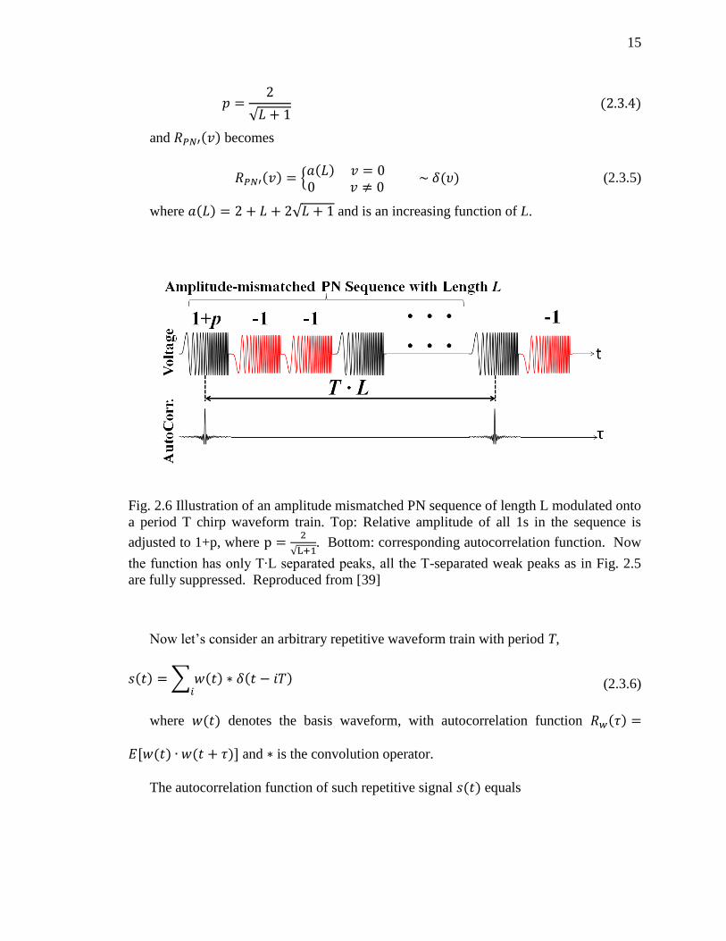
Fig. 2.6 Illustration of an amplitude mismatched PN sequence of length L modulated onto
a period T chirp waveform train. Top: Relative amplitude of all 1s in the sequence is
adjusted to 1+p, where p =2
√L+1. Bottom: corresponding autocorrelation function. Now
the function has only T∙L separated peaks, all the T-separated weak peaks as in Fig. 2.5
are fully suppressed. Reproduced from [39]
Now let’s consider an arbitrary repetitive waveform train with period T,
𝑠(𝑡) =∑ 𝑤(𝑡) ∗ 𝛿(𝑡 − 𝑖𝑇) 𝑖
(2.3.6)
where 𝑤(𝑡) denotes the basis waveform, with autocorrelation function 𝑅𝑤(𝜏) =
𝐸[𝑤(𝑡) ∙ 𝑤(𝑡 + 𝜏)] and ∗ is the convolution operator.
The autocorrelation function of such repetitive signal 𝑠(𝑡) equals
16
𝑅𝑠(𝜏) = 𝐸[𝑠(𝑡) ∙ 𝑠(𝑡 + 𝜏)]
= 𝐸 [∑ 𝑤(𝑡) ∗ 𝛿(𝑡 − 𝑖𝑇)𝑖
∑ 𝑤(𝑡) ∗ 𝛿(𝑡 − 𝑗𝑇 + 𝜏)𝑗
]
= ∑ ∑ 𝐸[𝑤(𝑡 − 𝑖𝑇) ∙ 𝑤(𝑡 − 𝑗𝑇 + 𝜏)]𝑗𝑖
= ∑ ∑ 𝑅𝑤𝑗
((𝑖 − 𝑗)𝑇 + 𝜏)𝑖
= ∑ 𝑅𝑤(𝜏 + 𝑘𝑇)𝑘
= ∑ 𝑅𝑤(𝜏) ∗ 𝛿(𝜏 + 𝑘𝑇)𝑘
(2.3.7)
Notice that the autocorrelation function of the repetitive signal 𝑠(𝑡)is merely the
autocorrelation function of the basis waveform 𝑅𝑤(𝜏) repeating every T.
When an arbitrary sequence 𝐶 is modulated onto the signal 𝑠(𝑡) at the same repetition
rate, the new waveform can be expressed as
𝑠′(𝑡) =∑ 𝐶𝑖 ∙ 𝑤(𝑡) ∗ 𝛿(𝑡 − 𝑖𝑇)𝑖
= ∑ 𝑤(𝑡) ∗ [𝐶𝑖 ∙ 𝛿(𝑡 − 𝑖𝑇)]𝑖
(2.3.8)
where 𝐶𝑖 is the i-th element in the sequence.
Evaluating the autocorrelation of the modulated signal reveals that
𝑅𝑠′(𝜏) = 𝐸[𝑠′(𝑡) ∙ 𝑠′(𝑡 + 𝜏)]
= 𝐸 [∑ 𝑤(𝑡) ∗ [𝐶𝑖 ∙ 𝛿(𝑡 − 𝑖𝑇)]𝑖
∑ 𝑤(𝑡) ∗ [𝐶𝑗∙𝛿(𝑡 − 𝑗𝑇 + 𝜏)]𝑗
]
= ∑ ∑ 𝐶𝑖𝐶𝑗𝐸[𝑤(𝑡 − 𝑖𝑇) ∙ 𝑤(𝑡 − 𝑗𝑇 + 𝜏)]𝑗𝑖
= ∑ ∑ 𝐶𝑖𝐶𝑗𝑅𝑤𝑗
((𝑖 − 𝑗)𝑇 + 𝜏)𝑖
17
= ∑ 𝑅𝑤[𝜏 + 𝑘𝑇]∑ 𝐶𝑖𝐶𝑖−𝑘𝑖𝑘
(2.3.9)
The last summation in Equation 2.3.9 over i is the discrete autocorrelation function of
the modulation sequence. Hence, if we set the modulation sequence to be the amplitude
mismatched PN sequence of length L as defined previously, Equ. 2.3.9 can be further
simplified as
𝑅𝑠′(𝜏) =∑ 𝑅𝑤[𝜏 + 𝑘𝐿𝑇]𝑘
= ∑ 𝑅𝑤(𝜏) ∗ 𝛿(𝜏 + 𝑘𝐿𝑇) 𝑘
(2.3.10)
Equation 2.3.10 clearly indicates that the autocorrelation function of a repetitive
waveform modulated by a length-L amplitude-mismatched PN sequence is the
autocorrelation function of the basis waveform repeated every L∙T. Compared with
equation 2.3.7, the PN sequence modulation increases the autocorrelation peak separation
exactly by a factor of the sequence length. As a result, by simply altering the length of
the modulation sequence, we are able to increase the time aperture of the waveform
arbitrarily.
One intriguing fact is that the basis waveform in above derivation is assumed to be
arbitrary. This implies that the amplitude-mismatched pseudorandom sequence can be
modulated onto any repetitive waveform to expand the temporal period.
Experimental Configuration
To experimentally implement the proposed Amplitude-mismatched Pseudorandom
Sequence Modulation, we design a photonic system based on differential detection. Our
experimental apparatus for RF arbitrary waveform generation is sketched in Fig. 2.7.
18
Overall our setup resembles the popular approach based on pulse shaping plus frequency-
to-time mapping, but modified for differential detection [46] and polarity switching. A
mode-locked fiber laser (Menlo Systems FC1500-250-WG) with 250 MHz repetition rate
and ~80 nm optical bandwidth (~ 1520 nm – 1600 nm) outputs an optical pulse train into
a commercial pulse shaper through an intermediate fiber amplifier (not shown in the
figure). The pulse shaper (FINISAR 1000S) has a resolution of ~10 GHz and ~5000
addressable pixels across an ~5 THz or 40 nm wavelength range (1527 nm – 1567 nm).
It is programmed using the Near-Field Frequency-to-Time Mapping (NFFTM) technique
[36], which pre-distorts both the amplitude and phase of the optical spectrum to achieve
target RF waveforms with high fidelity, while overcoming the “far-field” constraint
which otherwise may limit the maximum attainable RF bandwidth of the generated
waveform. After the shaper the signal is split equally into two arms through a 50-50
optical coupler. Synchronized to the laser repetition rate, a pattern generator provides
complementary drive signals to a pair of intensity modulators (IM). As a result the pulse
is transmitted in one arm and blocked in the other, with the transmitting arm selected
according to a preprogrammed PN sequence. The length of the dispersive fiber (~6.6km
of SMF-28 at ~17 ps/nm/km) is carefully chosen so that each 40-nm bandwidth spectrally
shaped pulse is stretched to a temporal duration of 4 ns, matched to the laser period.
With our differential detection geometry, it is important to ensure stable matching of both
the length and the dispersion experienced in each arm. Accordingly we designed a
dispersion block, illustrated in Fig. 2.8, in which both arms use the same piece of
dispersive fiber, but in a counter-propagating geometry implemented using a pair of
circulators. Both arms are provisioned with variable optical attenuators (not shown in the
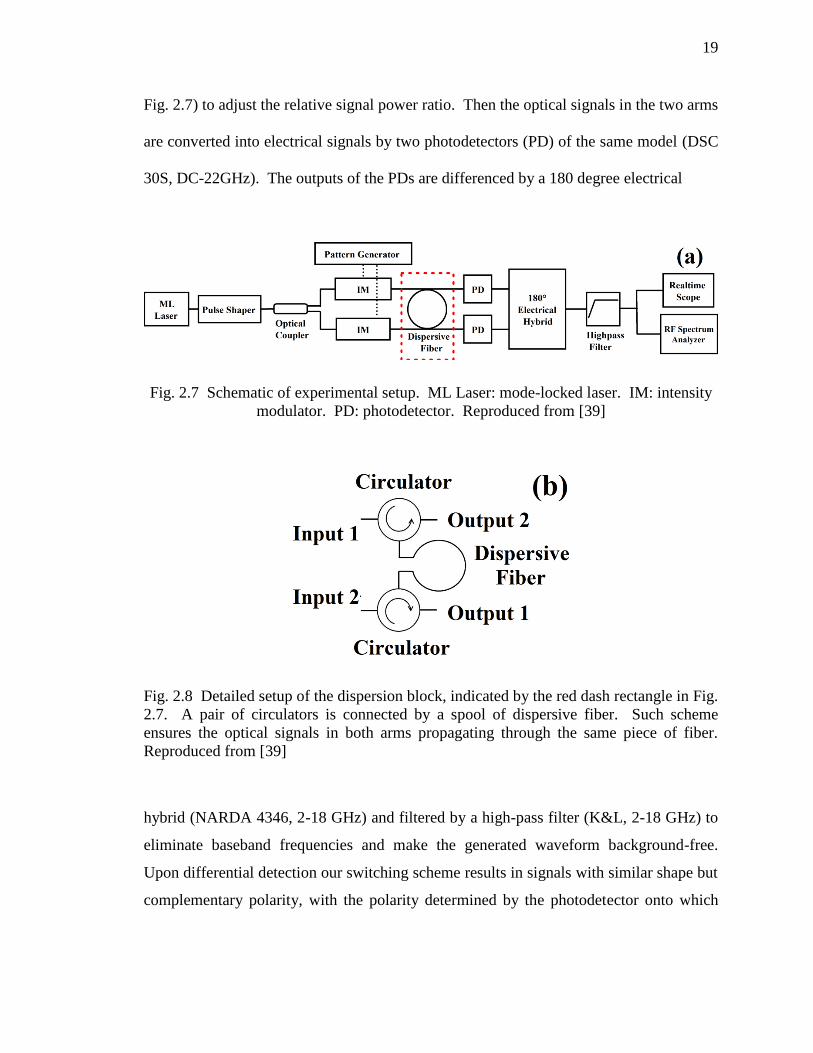
19
Fig. 2.7) to adjust the relative signal power ratio. Then the optical signals in the two arms
are converted into electrical signals by two photodetectors (PD) of the same model (DSC
30S, DC-22GHz). The outputs of the PDs are differenced by a 180 degree electrical
Fig. 2.7 Schematic of experimental setup. ML Laser: mode-locked laser. IM: intensity
modulator. PD: photodetector. Reproduced from [39]
Fig. 2.8 Detailed setup of the dispersion block, indicated by the red dash rectangle in Fig.
2.7. A pair of circulators is connected by a spool of dispersive fiber. Such scheme
ensures the optical signals in both arms propagating through the same piece of fiber.
Reproduced from [39]
hybrid (NARDA 4346, 2-18 GHz) and filtered by a high-pass filter (K&L, 2-18 GHz) to
eliminate baseband frequencies and make the generated waveform background-free.
Upon differential detection our switching scheme results in signals with similar shape but
complementary polarity, with the polarity determined by the photodetector onto which
20
light is incident during that switching cycle. Generated waveforms are measured in the
temporal domain by a real-time oscilloscope (Tektronix 72004B, 20GHz, 50 GS/s) with a
sampling period of 20 ps and in the frequency domain by an RF spectrum analyzer
(Agilent 8565EC).
Experimental Results
We first program the pulse shaper and select the amount of dispersion (~112.2 ps/nm)
such that each optical pulse is stretched into a linear down-chirp waveform covering the
frequency range from ~ 2 to 10 GHz. To generate as much power as possible, the
temporal duration of each waveform is set to be 4 ns, the same as the laser repetition
period. In this way, the generated waveform has a full duty cycle. Fig. 2.9 illustrates the
great correlation between the optical power spectrum, as shown in Fig. 2.9(a), and the
mapped waveform in temporal domain, as shown in Fig. 2.9(b). However, when
waveforms are scaled to higher bandwidth, such resemblance will disappear and NFFTM
becomes crucial [37]. For demonstration, a [1 -1 -1 1] sequence is modulated onto the
waveform and no amplitude adjustment is made. A temporal domain measurement of 16
ns, consisting of 4 linear down-chirped waveforms, is shown in Fig. 2.10. Suggested by
the polarity of each waveform labeled on top, the first and the last two chirps are of the
same polarity while the middle two are of the opposite polarity. To better demonstrate,
the first and the fourth chirped waveform in Fig. 2.10 are plotted in the same temporal
frame of 4 ns in Fig. 2.11. As clearly seen, waveforms with the same polarity are almost
identical in terms of amplitude and timing. In comparison, the first and the second
chirped waveform in Fig. 2.10, which are of opposite polarities, are also overlapped in
the same temporal frame of 4 ns. As we can see in Fig. 2.12, opposite polarity
waveforms are well-aligned in terms of timing.
21
Fig. 2.9 Demonstration of frequency-to-time mapping. Reproduced from [39]. (a)
Optical spectrum shaped with a linear period-increased sinusoidal amplitude modulation.
(b) Corresponding RF waveform after propagation through dispersion and optical-to-
electrical conversion.
Fig. 2.10 Experimental results of generated RF waveforms. Temporal measurement of
16 ns consisting of 4 down-chirped waveforms with polarities labeled on top.
22
Fig. 2.11 1st and 4
th chirped waveforms of the same polarity in Fig. 2.10 overlapped in a
temporal frame of 4 ns.
Fig. 2.12 1st and 2
nd chirped waveforms of the opposite polarities in Fig. 2.10 overlapped
in a temporal frame of 4 ns.
To exemplify the temporal period expansion due to waveform switching under PN
modulation, we set the length of the modulation sequence to be 15 and adjust the relative
signal amplitude of the two arms such that a ‘p’ value, as defined in Section 2.3.1, of ~0.6
is obtained. A temporal measurement is recorded over a span of 180 ns. For comparison,
23
a waveform is recorded over the same time span without waveform switching, as is done
in conventional FTM. Circular autocorrelation, defined for discrete function 𝑓[𝑛], 1 ≤
n ≤ N as
(𝑓𝑓)[𝑚] =
{
∑𝑓[𝑖] ∙ 𝑓[𝑖 + 𝑚]
𝑁
𝑖=1
𝑖𝑓 𝑖 + 𝑛 ≤ N
∑𝑓[𝑖] ∙ 𝑓[𝑖 + 𝑚 − 𝑁]
𝑁
𝑖=1
𝑖𝑓 𝑖 + 𝑛 > N
(2.3.11)
is computed off-line for both cases. Such correlation function can be used to evaluate a
chirp waveform in spread-spectrum ranging and related application. Specifically, the full-
width-half-maximum (FWHM) is proportional to the range resolution while the temporal
separation between correlation peaks indicates unambiguous detection range. As shown
in Fig. 2.13(a), the autocorrelation of the unmodulated waveform has a period of 4 ns, the
same as the laser repetition period. In contrast, as shown in Fig. 2.14(a), the waveform
switched according to a length-15 PN sequence has an autocorrelation with strong peaks
separated by 60 ns, corresponding to an increase in period by a factor of 15. Weak peaks
Fig. 2.13 (a) Computed autocorrelation function of unmodulated waveform, 4 ns between
correlation peaks. (b) Corresponding measured RF spectrum. Spectral line spacing is
250 MHz. Adapted from [39]
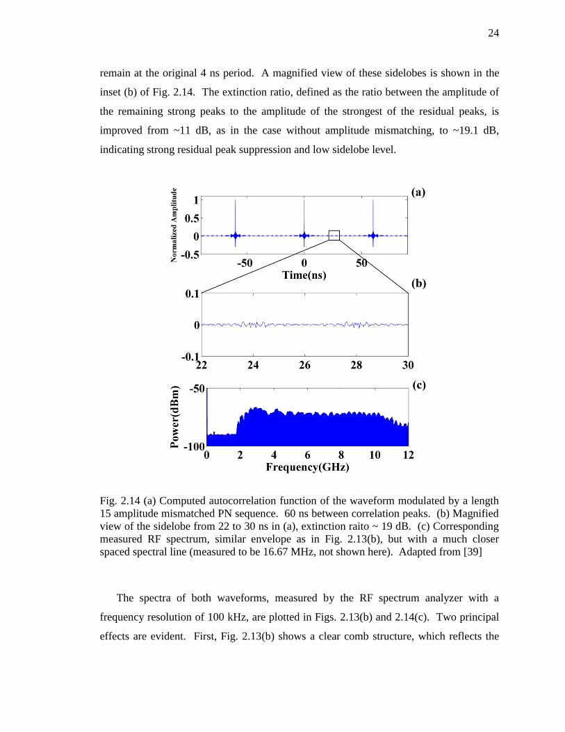
24
remain at the original 4 ns period. A magnified view of these sidelobes is shown in the
inset (b) of Fig. 2.14. The extinction ratio, defined as the ratio between the amplitude of
the remaining strong peaks to the amplitude of the strongest of the residual peaks, is
improved from ~11 dB, as in the case without amplitude mismatching, to ~19.1 dB,
indicating strong residual peak suppression and low sidelobe level.
Fig. 2.14 (a) Computed autocorrelation function of the waveform modulated by a length
15 amplitude mismatched PN sequence. 60 ns between correlation peaks. (b) Magnified
view of the sidelobe from 22 to 30 ns in (a), extinction raito ~ 19 dB. (c) Corresponding
measured RF spectrum, similar envelope as in Fig. 2.13(b), but with a much closer
spaced spectral line (measured to be 16.67 MHz, not shown here). Adapted from [39]
The spectra of both waveforms, measured by the RF spectrum analyzer with a
frequency resolution of 100 kHz, are plotted in Figs. 2.13(b) and 2.14(c). Two principal
effects are evident. First, Fig. 2.13(b) shows a clear comb structure, which reflects the
25
250 MHz waveform repetition frequency. The spectrum fills in Fig. 2.14(b), consistent
with the 15-fold decrease in waveform repetition frequency. Second, we observe that the
envelope of the RF spectrum is largely unaffected by the increase of the temporal period.
As stated previously, basis waveform generation and PN-modulated waveform switching
are separated in our technique. This enables us to increase the time-aperture and the RF
bandwidth simultaneously. By setting the length of the PN sequence to 1023 and
programing a higher rate chirp modulation on the optical power spectrum, we are able to
generate a waveform with more than 4 microseconds time aperture (see autocorrelation in
Fig. 2.15(a)) and a RF bandwidth of ~ 20 GHz (see RF spectrum in Fig. 2.15(b)). The
resulting TBP exceeds 80,000. The autocorrelation peaks have a FWHM of ~50ps,
making the ratio of peak spacing to peak-width ~80,000. The suppressed autocorrelation
peaks, with an extinction ratio of ~21dB, are too small to discern given the linear scale of
Fig. 2.15 (a).
Fig. 2.15 (a) Computed autocorrelation function of the waveform modulated with a
length 1023 amplitude mismatched PN sequence. Separation between correlation peaks
is 4092 ns. (b) Corresponding measured RF spectrum with smooth and flat envelope up
to 20 GHz. Spectral line spacing is measured to be ~ 244 kHz (not shown here).
Adapted from [39]
Our technique also exhibits great performance in stability and repeatability. Because
our hybrid optical-electrical design combines signals in electrical domain instead of
26
optical domain, the system is insensitive to the relative optical phases of the two
generation arms in Fig. 2.7. Moreover, the dispersion block described in Fig. 2.8
provides signals in both arms with the same propagation environment. Thus, any
distortions, e.g. temperature, fluctuation, are experienced in the same way by the two
arms. As a result, the consequential distortion difference can be eliminated to a large
extent. Last but not the least, a clock obtained from a GPS signal is employed to
precisely stabilize the repetition rate of the utilized mode locked laser. Consequently, our
generated waveforms have low timing jitter. To quantify the stability and repeatability
performance, a long-term measurement is conducted. 336 temporal measurements of
signal described in Fig. 2.10 are recorded over one hour. The first measurement is
chosen as the reference and cross-correlation functions between the reference and all
other measurements are computed off-line. All 335 cross-correlation functions are
overlapped in the same 4 ns temporal frame in Fig. 2.16(b). Clearly, all the cross-
correlations are very similar. Compared with the autocorrelation of the reference
measurement, as shown in Fig. 2.16(a), the curve in Fig. 2.16(b) is slightly thicker
because of the amplitude differences between each cross-correlation. Minor distortions
may also be seen at both main negative sidelobes. These results provide compelling
Fig. 2.16 Long term measurement results. (a) Autocorrelation function of the reference
measurement. (b) Cross-correlation functions between the reference and all other
measurements. 335 traces overlapped in a temporal frame of 4 ns. Reproduced from
[39]
27
evidence of stable waveform generation. Consequently, data averaging can be
implemented to reduce the additive noise in channel sounding and other applications.
Furthermore, the reference waveform may be stored and used in later experiments as a
template for pulse compression via offline correlation processing.
2.4. Dual-Shaper Photonic RF-AWG
Experimental Configuration
Introduced in last section, a differential detection scheme enables the generation of
arbitrary wideband RF waveforms and the implementation of amplitude-mismatched
pseudorandom sequence modulation. However, limited by the bandwidth of the
differential photodetector, this scheme offers the synthesis of waveforms only up to ~ 20
GHz, with which the electrical counterpart is comparable. It will be of great interests if
only a traditional photodetector with one input is needed in the setup, for the reason that
high-bandwidth (> 20 GHz) balanced photodetectors and/or photodetectors combined
with electrical hybrid are either unavailable or costly. To further increase the RF
bandwidth of the generated waveforms, a new experimental apparatus is proposed and
sketched in Fig. 2.17.
Fig. 2.17 Sketch of the experimental setup of Dual-shaper RF-AWG. PD: photodetector.
PC: polarization controller. PBS: polarization beam splitter. IM: intensity modulator.
28
The setup starts with a commercial mode-locked fiber laser (Menlo System, FC1500-
250-WG) which has a repetition rate of 250 MHz and ~ 80 nm optical bandwidth (~ 1520
– 1600 nm). The output optical pulse train from the laser is amplified and then split
equally into two arms by a 50-50 optical coupler. Two pulse shapers (Finisar 1000S,
~5000 addressable pixels, ~ 500 independent controllable pixel group) with ~ 10 GHz
resolution across ~ 40 nm wavelength range (~1527 nm – 1567 nm) are programmed to
provide linear chirp modulation on the spectra of the optical signals in both arms. Since
the two pulse shapers are independently controlled, their modulations can be either
complementary to realize amplitude-mismatched PN modulation or complementary with
pre-defined phase shift for phase shifted PN modulation. Spectrally shaped optical pulses
are then sent into intensity modulators through intermediate amplification. The two
intensity modulators are driven complementarily by a pattern generator which is
synchronized with the source laser and pre-programmed with a PN sequence. Within any
laser period, only one of the arms is open and the other is blocked. Such a
complementary on-off modulator, together with the 50-50 splitter in the beginning,
functions as an optical path switch that directs pulses coming out from the laser into
either arm according to the pre-programmed PN sequence. After the intensity
modulators, optical signals in both arms are combined through a fiber polarization beam
splitter. The polarizations of the signals are adjusted to be perpendicular to ensure
minimum interference. Subsequently, the combined signal propagates through ~ 6.6 km
of single mode fiber (SMF-28, ~ 110 ps/nm dispersion in total) and impinges on a high
speed 50 GHz photodetector (U2T XPDV2020R-VF-FP). Generated waveforms are
measured in the temporal domain by either a real-time oscilloscope (Tektronix 72004B,
20GHz, 50 GS/s) with a sampling period of 20 ps or a digital serial analyzer (Tektronix
DSA 8200, 65 GHz ) with a sampling period of 5ps and in the frequency domain by an
RF spectrum analyzer (Agilent 8565EC).
Experimental Validations
To verify this new scheme, we first repeat the amplitude-mismatched modulation
demonstrations presented in Section 2.3. The two pulse shapers are programmed with
29
linear chirp modulations with anti-phase, which in the end results in similar chirp
waveform but with opposite polarity. The waveforms span a frequency range from ~ DC
to 20 GHz, with ~ 4 ns temporal duration. To compare with the waveform presented in
Section 2.3.3, the length of the PN sequence is also set to 15 and relative amplitude
adjustment is made. A temporal measurement of 180 ns is recorded via the real-time
scope. 20 ns of the data is acquired and plotted in Fig. 2.18, where we can clearly see the
amplitude mismatch between each set of basis chirp waveforms. To better illustrate, the
first and second basis chirp waveforms are overlapped in the temporal frame of 4 ns, as
shown in Fig. 2.19. The dips of one waveform are almost exactly aligned with the peaks
of the other one, indicating the same rate of chirping but with opposite polarities.
Circular autocorrelation, as defined in Section 2.3.3, of the measured data is computed
and depicted in Fig. 2.20. As we expected, the autocorrelation function consists of 60 ns
separated strong peaks along with the original 4-ns repeating peaks severely attenuated.
With the help of the magnified view of the sidelobe, as shown in the inset of Fig. 2.20,
we determine an extinction ratio ~ 19 dB (in terms of auto-correlation amplitude), almost
exactly as that in the case of the differential detection scheme. Furthermore, we obtain
the RF spectrum of the generated waveform from the spectral analyzer, together with that
of the waveform without any PN modulation as a comparison. Similar to what we have
in Section 2.3.3, the spectrum of the PN modulated waveform has preserved envelope but
greatly reduced (measured to be exactly 15 fold) spectral line spacing compared with that
of the unmodulated ones, as shown in Fig. 2.21. These experimental results confirm that
the dual-shaper scheme is able to deliver time aperture expanded RF waveforms in a very
similar way as the differential detection scheme.
30
Fig. 2.18 Experimental measurement of linear chirped waveform modulated with
amplitude mismatched PN sequence. Five basis waveforms in a span of 20 ns.
Fig. 2.19 1st and 2
nd basis linear chirped waveforms in Fig. 2.18 overlapped in a temporal
frame of 4 ns. Dips from one waveform are aligned with corresponding peaks of the
other, indicating the same chirping profile but opposite polarity.
31
Fig. 2.20 Computed autocorrelation function of a 180 ns measurement of a linear chirped
waveform modulated with a length-15 amplitude mismatched PN sequence. 60 ns
between correlation peaks. Inset: magnified view of the sidelobe level from 22 to 30 ns.
Extinction ratio ~ 19 dB
Fig. 2.21 Measured RF spectra of the generated linear chirped waveform. Top: with
length-15 PN sequence modulation. Bottom: without any modulation
32
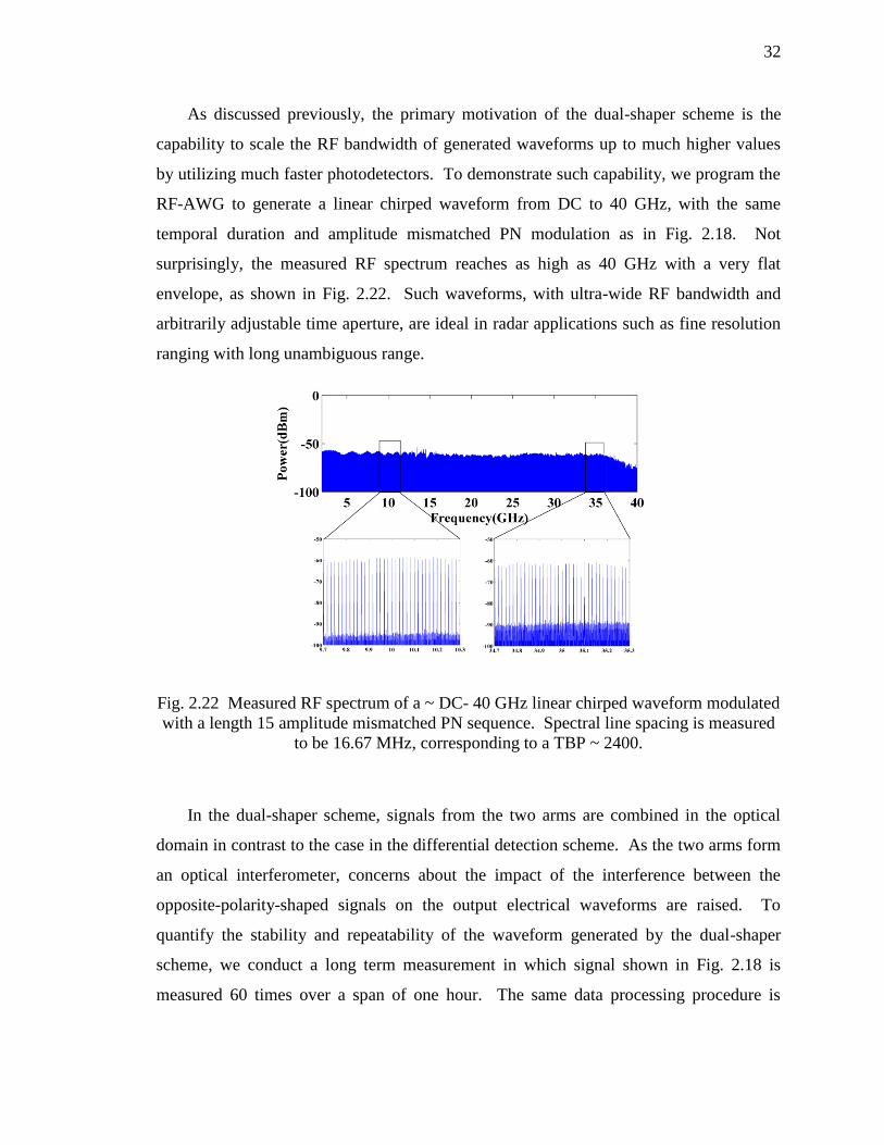
As discussed previously, the primary motivation of the dual-shaper scheme is the
capability to scale the RF bandwidth of generated waveforms up to much higher values
by utilizing much faster photodetectors. To demonstrate such capability, we program the
RF-AWG to generate a linear chirped waveform from DC to 40 GHz, with the same
temporal duration and amplitude mismatched PN modulation as in Fig. 2.18. Not
surprisingly, the measured RF spectrum reaches as high as 40 GHz with a very flat
envelope, as shown in Fig. 2.22. Such waveforms, with ultra-wide RF bandwidth and
arbitrarily adjustable time aperture, are ideal in radar applications such as fine resolution
ranging with long unambiguous range.
Fig. 2.22 Measured RF spectrum of a ~ DC- 40 GHz linear chirped waveform modulated
with a length 15 amplitude mismatched PN sequence. Spectral line spacing is measured
to be 16.67 MHz, corresponding to a TBP ~ 2400.
In the dual-shaper scheme, signals from the two arms are combined in the optical
domain in contrast to the case in the differential detection scheme. As the two arms form
an optical interferometer, concerns about the impact of the interference between the
opposite-polarity-shaped signals on the output electrical waveforms are raised. To
quantify the stability and repeatability of the waveform generated by the dual-shaper
scheme, we conduct a long term measurement in which signal shown in Fig. 2.18 is
measured 60 times over a span of one hour. The same data processing procedure is
33
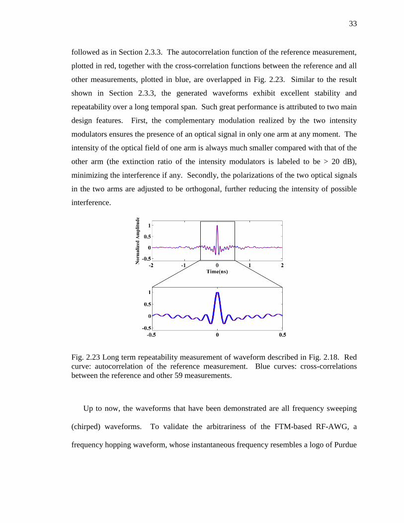
followed as in Section 2.3.3. The autocorrelation function of the reference measurement,
plotted in red, together with the cross-correlation functions between the reference and all
other measurements, plotted in blue, are overlapped in Fig. 2.23. Similar to the result
shown in Section 2.3.3, the generated waveforms exhibit excellent stability and
repeatability over a long temporal span. Such great performance is attributed to two main
design features. First, the complementary modulation realized by the two intensity
modulators ensures the presence of an optical signal in only one arm at any moment. The
intensity of the optical field of one arm is always much smaller compared with that of the
other arm (the extinction ratio of the intensity modulators is labeled to be > 20 dB),
minimizing the interference if any. Secondly, the polarizations of the two optical signals
in the two arms are adjusted to be orthogonal, further reducing the intensity of possible
interference.
Fig. 2.23 Long term repeatability measurement of waveform described in Fig. 2.18. Red
curve: autocorrelation of the reference measurement. Blue curves: cross-correlations
between the reference and other 59 measurements.
Up to now, the waveforms that have been demonstrated are all frequency sweeping
(chirped) waveforms. To validate the arbitrariness of the FTM-based RF-AWG, a
frequency hopping waveform, whose instantaneous frequency resembles a logo of Purdue
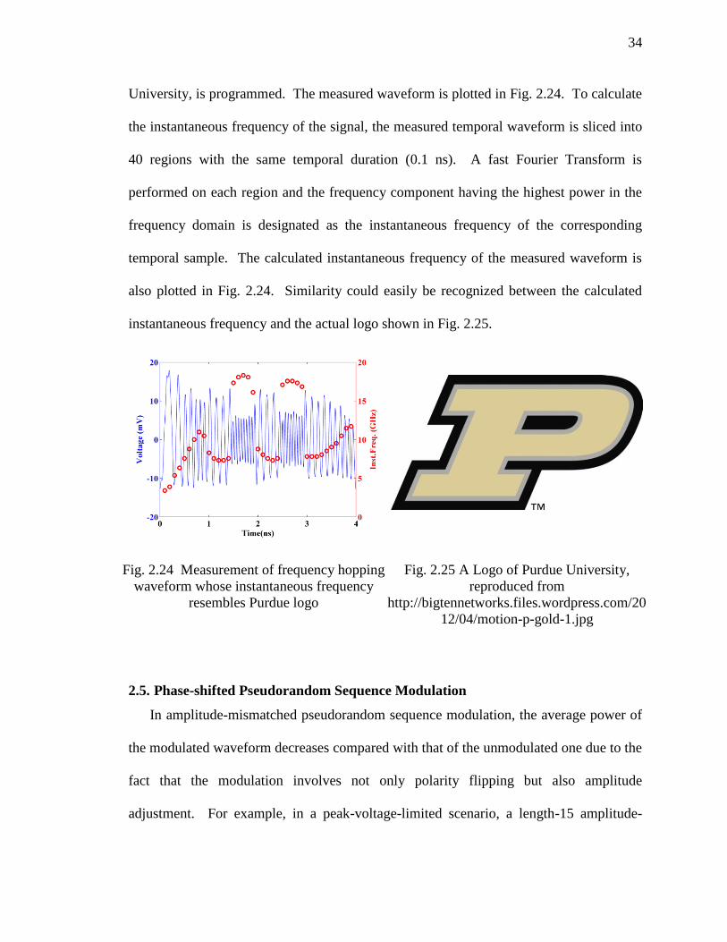
34
University, is programmed. The measured waveform is plotted in Fig. 2.24. To calculate
the instantaneous frequency of the signal, the measured temporal waveform is sliced into
40 regions with the same temporal duration (0.1 ns). A fast Fourier Transform is
performed on each region and the frequency component having the highest power in the
frequency domain is designated as the instantaneous frequency of the corresponding
temporal sample. The calculated instantaneous frequency of the measured waveform is
also plotted in Fig. 2.24. Similarity could easily be recognized between the calculated
instantaneous frequency and the actual logo shown in Fig. 2.25.
Fig. 2.24 Measurement of frequency hopping
waveform whose instantaneous frequency
resembles Purdue logo
Fig. 2.25 A Logo of Purdue University,
reproduced from
http://bigtennetworks.files.wordpress.com/20
12/04/motion-p-gold-1.jpg
2.5. Phase-shifted Pseudorandom Sequence Modulation
In amplitude-mismatched pseudorandom sequence modulation, the average power of
the modulated waveform decreases compared with that of the unmodulated one due to the
fact that the modulation involves not only polarity flipping but also amplitude
adjustment. For example, in a peak-voltage-limited scenario, a length-15 amplitude-
35
mismatched pseudorandom sequence modulated linear chirp has ~ 30% less average
power than the maximum achievable value. New modulation techniques that offer the
maximum achievable average power are of great interest. Moreover, the introduction of
a dual-shaper scheme enables the exploration of basis waveforms other than anti-polarity
ones. Taking advantage of these new degrees of freedom, we propose another
modulation technique named phase-shifted pseudorandom sequence modulation.
As sketched in Fig. 2.5, polarity-flipping of a basis waveform is equivalent to adding
a 𝜋 phase shift to the basis waveform. Now, if we slightly detune the phase shift from 𝜋,
we can also achieve a perfect autocorrelation with zero correlation floor as described in
the amplitude-mismatched scheme. Mathematically, the phase-shifted pseudorandom
sequence can be expressed as,
𝑃𝑁′′[𝑖] =1 + 𝑒𝑗𝜑
2∙ 𝑃𝑁[𝑖] +
1 − 𝑒𝑗𝜑
2∙ 𝑈[𝑖], 𝑖 = 1, 2, … , 𝐿 (2.5.1)
where 𝑃𝑁 and 𝑈 are defined in the same way as in Section 2.3.1, 𝐿 is the length of the
sequence and 𝜑 is a constant phase shift. As a result, 𝑃𝑁′′[𝑖] follows the same pattern as
𝑃𝑁[𝑖] except that instead of having a phase shift of 𝜋 at certain positions, it exhibits
phase shift of 𝜋 + 𝜑. The discrete circular autocorrelation function of this complex-
valued sequence can be expressed as
𝑅𝑃𝑁′′(𝜐) = 𝑃𝑁′′ 𝑃𝑁′′
=1+cos𝜑
2∙ 𝑃𝑁𝑃𝑁 +
1−cos𝜑
2∙ 𝑈 𝑈 +
𝑗 sin𝜑
2∙ 𝑃𝑁 𝑈 −
𝑗 sin𝜑
2∙ 𝑈𝑃𝑁
(2.5.2)
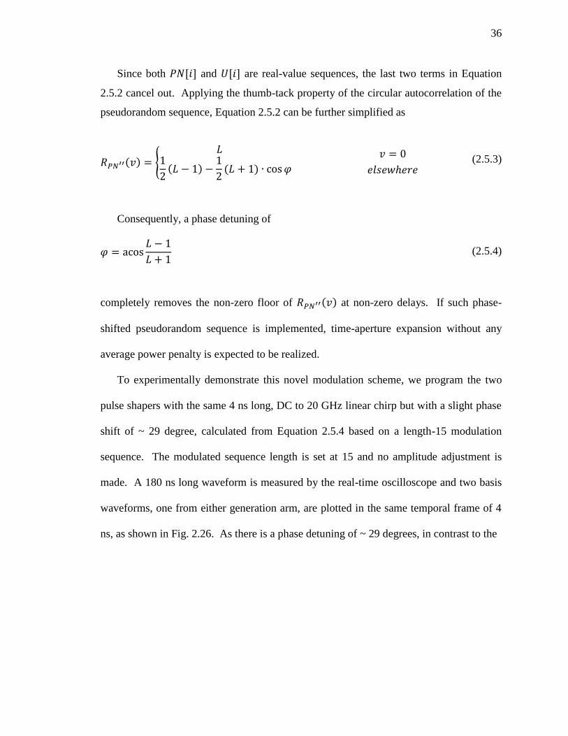
36
Since both 𝑃𝑁[𝑖] and 𝑈[𝑖] are real-value sequences, the last two terms in Equation
2.5.2 cancel out. Applying the thumb-tack property of the circular autocorrelation of the
pseudorandom sequence, Equation 2.5.2 can be further simplified as
𝑅𝑃𝑁′′(𝑣) = {𝐿
1
2(𝐿 − 1) −
1
2(𝐿 + 1) ∙ cos𝜑
𝑣 = 0
𝑒𝑙𝑠𝑒𝑤ℎ𝑒𝑟𝑒 (2.5.3)
Consequently, a phase detuning of
𝜑 = acos𝐿 − 1
𝐿 + 1 (2.5.4)
completely removes the non-zero floor of 𝑅𝑃𝑁′′(𝑣) at non-zero delays. If such phase-
shifted pseudorandom sequence is implemented, time-aperture expansion without any
average power penalty is expected to be realized.
To experimentally demonstrate this novel modulation scheme, we program the two
pulse shapers with the same 4 ns long, DC to 20 GHz linear chirp but with a slight phase
shift of ~ 29 degree, calculated from Equation 2.5.4 based on a length-15 modulation
sequence. The modulated sequence length is set at 15 and no amplitude adjustment is
made. A 180 ns long waveform is measured by the real-time oscilloscope and two basis
waveforms, one from either generation arm, are plotted in the same temporal frame of 4
ns, as shown in Fig. 2.26. As there is a phase detuning of ~ 29 degrees, in contrast to the
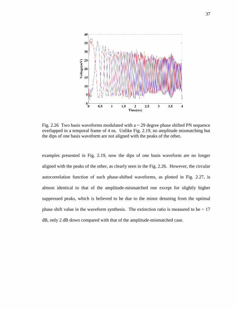
37
Fig. 2.26 Two basis waveforms modulated with a ~ 29 degree phase shifted PN sequence
overlapped in a temporal frame of 4 ns. Unlike Fig. 2.19, no amplitude mismatching but
the dips of one basis waveform are not aligned with the peaks of the other.
examples presented in Fig. 2.19, now the dips of one basis waveform are no longer
aligned with the peaks of the other, as clearly seen in the Fig. 2.26. However, the circular
autocorrelation function of such phase-shifted waveforms, as plotted in Fig. 2.27, is
almost identical to that of the amplitude-mismatched one except for slightly higher
suppressed peaks, which is believed to be due to the minor detuning from the optimal
phase shift value in the waveform synthesis. The extinction ratio is measured to be ~ 17
dB, only 2 dB down compared with that of the amplitude-mismatched case.
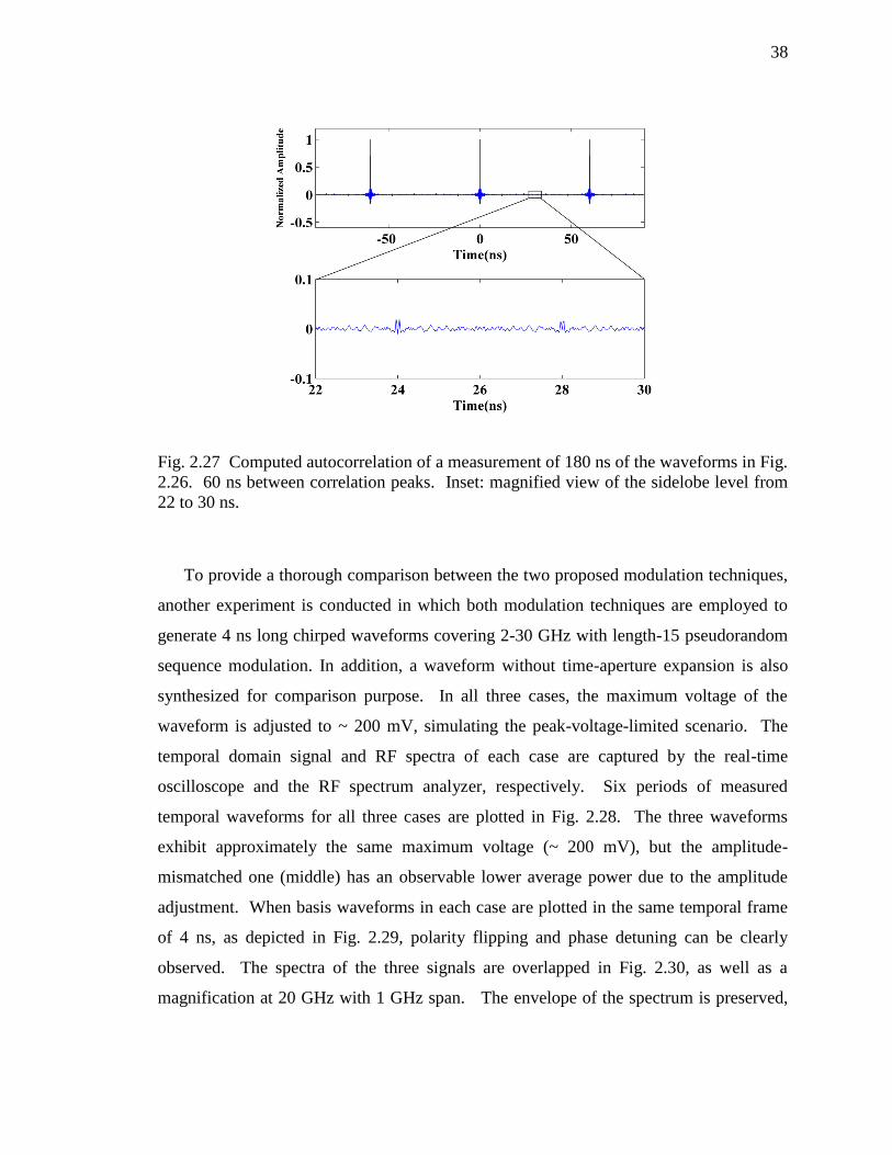
38
Fig. 2.27 Computed autocorrelation of a measurement of 180 ns of the waveforms in Fig.
2.26. 60 ns between correlation peaks. Inset: magnified view of the sidelobe level from
22 to 30 ns.
To provide a thorough comparison between the two proposed modulation techniques,
another experiment is conducted in which both modulation techniques are employed to
generate 4 ns long chirped waveforms covering 2-30 GHz with length-15 pseudorandom
sequence modulation. In addition, a waveform without time-aperture expansion is also
synthesized for comparison purpose. In all three cases, the maximum voltage of the
waveform is adjusted to ~ 200 mV, simulating the peak-voltage-limited scenario. The
temporal domain signal and RF spectra of each case are captured by the real-time
oscilloscope and the RF spectrum analyzer, respectively. Six periods of measured
temporal waveforms for all three cases are plotted in Fig. 2.28. The three waveforms
exhibit approximately the same maximum voltage (~ 200 mV), but the amplitude-
mismatched one (middle) has an observable lower average power due to the amplitude
adjustment. When basis waveforms in each case are plotted in the same temporal frame
of 4 ns, as depicted in Fig. 2.29, polarity flipping and phase detuning can be clearly
observed. The spectra of the three signals are overlapped in Fig. 2.30, as well as a
magnification at 20 GHz with 1 GHz span. The envelope of the spectrum is preserved,
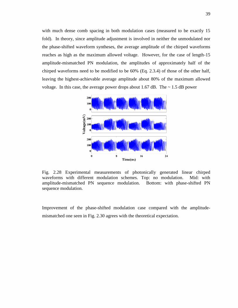
39
with much dense comb spacing in both modulation cases (measured to be exactly 15
fold). In theory, since amplitude adjustment is involved in neither the unmodulated nor
the phase-shifted waveform syntheses, the average amplitude of the chirped waveforms
reaches as high as the maximum allowed voltage. However, for the case of length-15
amplitude-mismatched PN modulation, the amplitudes of approximately half of the
chirped waveforms need to be modified to be 60% (Eq. 2.3.4) of those of the other half,
leaving the highest-achievable average amplitude about 80% of the maximum allowed
voltage. In this case, the average power drops about 1.67 dB. The ~ 1.5 dB power
Fig. 2.28 Experimental measurements of photonically generated linear chirped
waveforms with different modulation schemes. Top: no modulation. Mid: with
amplitude-mismatched PN sequence modulation. Bottom: with phase-shifted PN
sequence modulation.
Improvement of the phase-shifted modulation case compared with the amplitude-
mismatched one seen in Fig. 2.30 agrees with the theoretical expectation.
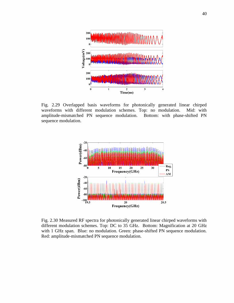
40
Fig. 2.29 Overlapped basis waveforms for photonically generated linear chirped
waveforms with different modulation schemes. Top: no modulation. Mid: with
amplitude-mismatched PN sequence modulation. Bottom: with phase-shifted PN
sequence modulation.
Fig. 2.30 Measured RF spectra for photonically generated linear chirped waveforms with
different modulation schemes. Top: DC to 35 GHz. Bottom: Magnification at 20 GHz
with 1 GHz span. Blue: no modulation. Green: phase-shifted PN sequence modulation.
Red: amplitude-mismatched PN sequence modulation.
41
2.6. Arbitrary Waveform Generation in W-band [47]
As discussed previously in the Introduction, the W-band (75-110 GHz) offers a
number of potentials in high resolution detection and high-speed communications, yet
remains largely unexploited primarily due to the lack of versatile waveform generation.
Due to the speed limitation of digital-to-analog converters (DAC), direct generation of
arbitrary signals at frequencies in the range of 100 GHz and above is not a possibility
using state-of-the-art electronics. Also, up-conversion [13, 48, 49] of electronically-
generated arbitrary baseband signals would still have bandwidth constraints - bounded by
the intermediate frequency (IF) bandwidth of the mixer - and suffer severely from issues
like timing jitter, electromagnetic interference (EMI), and bulkiness [50, 51]. These
shortcomings have motivated researchers to pursue the possibility of photonic-assisted
RF generation, which not only can provide broad bandwidths, but also exceptionally low
timing jitter and phase-noise performance [52, 53], immunity to EMI, cost-effective and
low propagation loss radio-over-fiber signal distribution, and the possibility of on-chip
integration [50, 51]. However, there has been no previous report on the synthesis of
arbitrary W-band waveforms. In this part of our work, by utilizing the aforementioned
dual-shaper scheme and an ultra-high-speed photodetector, we extend the frequency of
the generated waveform up to W-band. In the meantime, as the time aperture expansion
and the waveform generation are completely separated in our technique, amplitude-
mismatched pseudorandom sequence modulation is also implemented to provide the
generated waveform with an arbitrary time aperture.
One of the most decisive limiting factors of the bandwidth of the photonically
generated arbitrary waveform is the speed of optical to electrical conversion. In this
work, we receive a specially-engineered ultra-high-speed photodetector fabricated by our
42
collaborators from the National Central University in Taiwan. This high-power near-
ballistic uni-travelling-carrier photodetector (NBUTC-PD) with a 5 𝜇𝑚 active diameter
has a 175 GHz optical-to-electrical (O-E) 3dB bandwidth and saturation current of ~16
mA. Compared with the device structure reported in the previous work [54], here the p-
type In0.53GaAs absorption layer thickness has been increased from 160 to 260 nm.
This improves the DC responsivity, which now reaches ~0.25 A/W, and saves the
required optical power during high-output-power operation. In addition, the n-type InP
collector layer thickness has been increased from 180 to 310 nm in order to relax the
limitation on the maximum allowable device active diameter (> 5 𝜇𝑚) for the desired
RC-limited bandwidth (200 GHz). A larger device active diameter improves the
tolerance in optical alignment during system measurement.
Experimental Configuration
Since even the lower bound of W-band (75 GHz) exceeds the capability of the
measurement instruments available in our lab, a special design is implemented to capture
the generated waveform, as depicted in Fig. 2.31. The photonic RF-AWG remains the
same as described in Fig. 2.17. To scale the frequency of the generated waveform to W-
band, NFFTM is implemented. We must notice that, NFFTM is essentially a baseband
generation technique, which implies that it is the highest frequency that should be
considered for the time-bandwidth product limitation. As mentioned previously in
Section 2.2, the time-bandwidth of the generated waveform based on optical pulse
shaping is ultimately restricted by the number of resolvable pulse shaping element
utilized. The pulse shapers employed in the setup have ~ 500 resolvable pulse shaping
element. Consequently, the temporal duration of the generated W-band waveform cannot
exceed ~ 2.2 nanoseconds using NFFTM. Based on such analysis, we replace the 6.6 km
of single mode fiber with a spool of 3.3 km, reducing the time aperture of each stretched
optical pulse to ~ 2 ns.
Optically-tailored waveforms from the photonic RF-AWG setups are directed to the
NBUTC-PD based photonic-transmitter mixer (PTM) [8, 55]. Detailed photographs of
the PTM chip as well as the optical and electrical instrumentation apparatus are shown in
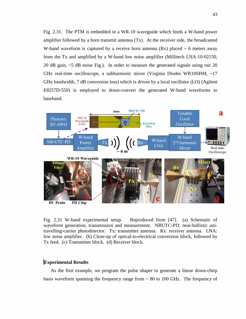
43
Fig. 2.31. The PTM is embedded in a WR-10 waveguide which feeds a W-band power
amplifier followed by a horn transmit antenna (Tx). At the receiver side, the broadcasted
W-band waveform is captured by a receive horn antenna (Rx) placed ~ 6 meters away
from the Tx and amplified by a W-band low noise amplifier (Millitech LNA-10-02150,
20 dB gain, ~5 dB noise Fig.). In order to measure the generated signals using our 20
GHz real-time oscilloscope, a subharmonic mixer (Virginia Diodes WR10SHM, ~17
GHz bandwidth, 7 dB conversion loss) which is driven by a local oscillator (LO) (Agilent
E8257D-550) is employed to down-convert the generated W-band waveforms to
baseband.
Fig. 2.31 W-band experimental setup. Reproduced from [47]. (a) Schematic of
waveform generation, transmission and measurement. NBUTC-PD: near-ballistic uni-
travelling-carrier photodetector. Tx: transmitter antenna. Rx: receiver antenna. LNA:
low noise amplifier. (b) Close-up of optical-to-electrical conversion block, followed by
Tx feed. (c) Transmitter block. (d) Receiver block.
Experimental Results
As the first example, we program the pulse shaper to generate a linear down-chirp
basis waveform spanning the frequency range from ~ 80 to 100 GHz. The frequency of
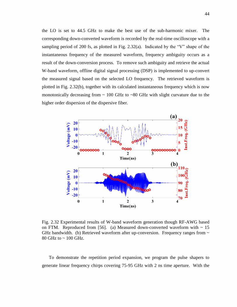
44
the LO is set to 44.5 GHz to make the best use of the sub-harmonic mixer. The
corresponding down-converted waveform is recorded by the real-time oscilloscope with a
sampling period of 200 fs, as plotted in Fig. 2.32(a). Indicated by the “V” shape of the
instantaneous frequency of the measured waveform, frequency ambiguity occurs as a
result of the down-conversion process. To remove such ambiguity and retrieve the actual
W-band waveform, offline digital signal processing (DSP) is implemented to up-convert
the measured signal based on the selected LO frequency. The retrieved waveform is
plotted in Fig. 2.32(b), together with its calculated instantaneous frequency which is now
monotonically decreasing from ~ 100 GHz to ~80 GHz with slight curvature due to the
higher order dispersion of the dispersive fiber.
Fig. 2.32 Experimental results of W-band waveform generation though RF-AWG based
on FTM. Reproduced from [56]. (a) Measured down-converted waveform with ~ 15
GHz bandwidth. (b) Retrieved waveform after up-conversion. Frequency ranges from ~
80 GHz to ~ 100 GHz.
To demonstrate the repetition period expansion, we program the pulse shapers to
generate linear frequency chirps covering 75-95 GHz with 2 ns time aperture. With the
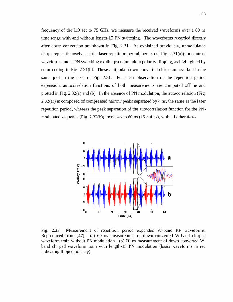
45
frequency of the LO set to 75 GHz, we measure the received waveforms over a 60 ns
time range with and without length-15 PN switching. The waveforms recorded directly
after down-conversion are shown in Fig. 2.31. As explained previously, unmodulated
chirps repeat themselves at the laser repetition period, here 4 ns (Fig. 2.31(a)); in contrast
waveforms under PN switching exhibit pseudorandom polarity flipping, as highlighted by
color-coding in Fig. 2.31(b). These antipodal down-converted chirps are overlaid in the
same plot in the inset of Fig. 2.31. For clear observation of the repetition period
expansion, autocorrelation functions of both measurements are computed offline and
plotted in Fig. 2.32(a) and (b). In the absence of PN modulation, the autocorrelation (Fig.
2.32(a)) is composed of compressed narrow peaks separated by 4 ns, the same as the laser
repetition period, whereas the peak separation of the autocorrelation function for the PN-
modulated sequence (Fig. 2.32(b)) increases to 60 ns (15 × 4 ns), with all other 4-ns-
Fig. 2.33 Measurement of repetition period expanded W-band RF waveforms.
Reproduced from [47]. (a) 60 ns measurement of down-converted W-band chirped
waveform train without PN modulation. (b) 60 ns measurement of down-converted W-
band chirped waveform train with length-15 PN modulation (basis waveforms in red
indicating flipped polarity).
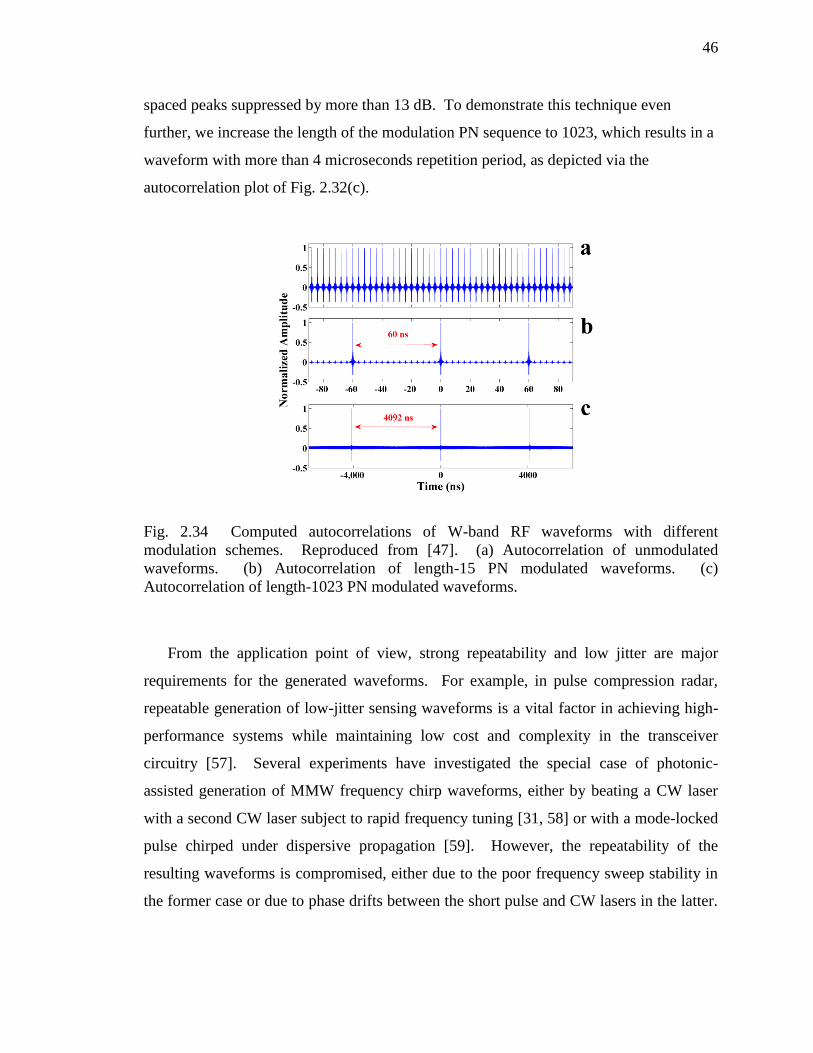
46
spaced peaks suppressed by more than 13 dB. To demonstrate this technique even
further, we increase the length of the modulation PN sequence to 1023, which results in a
waveform with more than 4 microseconds repetition period, as depicted via the
autocorrelation plot of Fig. 2.32(c).
Fig. 2.34 Computed autocorrelations of W-band RF waveforms with different
modulation schemes. Reproduced from [47]. (a) Autocorrelation of unmodulated
waveforms. (b) Autocorrelation of length-15 PN modulated waveforms. (c)
Autocorrelation of length-1023 PN modulated waveforms.
From the application point of view, strong repeatability and low jitter are major
requirements for the generated waveforms. For example, in pulse compression radar,
repeatable generation of low-jitter sensing waveforms is a vital factor in achieving high-
performance systems while maintaining low cost and complexity in the transceiver
circuitry [57]. Several experiments have investigated the special case of photonic-
assisted generation of MMW frequency chirp waveforms, either by beating a CW laser
with a second CW laser subject to rapid frequency tuning [31, 58] or with a mode-locked
pulse chirped under dispersive propagation [59]. However, the repeatability of the
resulting waveforms is compromised, either due to the poor frequency sweep stability in
the former case or due to phase drifts between the short pulse and CW lasers in the latter.
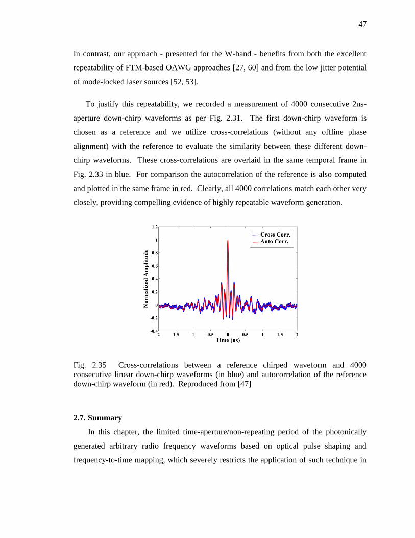
47
In contrast, our approach - presented for the W-band - benefits from both the excellent
repeatability of FTM-based OAWG approaches [27, 60] and from the low jitter potential
of mode-locked laser sources [52, 53].
To justify this repeatability, we recorded a measurement of 4000 consecutive 2ns-
aperture down-chirp waveforms as per Fig. 2.31. The first down-chirp waveform is
chosen as a reference and we utilize cross-correlations (without any offline phase
alignment) with the reference to evaluate the similarity between these different down-
chirp waveforms. These cross-correlations are overlaid in the same temporal frame in
Fig. 2.33 in blue. For comparison the autocorrelation of the reference is also computed
and plotted in the same frame in red. Clearly, all 4000 correlations match each other very
closely, providing compelling evidence of highly repeatable waveform generation.
Fig. 2.35 Cross-correlations between a reference chirped waveform and 4000
consecutive linear down-chirp waveforms (in blue) and autocorrelation of the reference
down-chirp waveform (in red). Reproduced from [47]
2.7. Summary
In this chapter, the limited time-aperture/non-repeating period of the photonically
generated arbitrary radio frequency waveforms based on optical pulse shaping and
frequency-to-time mapping, which severely restricts the application of such technique in
48
spread-spectrum channel sounding, chirped radar, etc., is discussed. Two novel
modulation techniques, amplitude-mismatched and phase-shifted pseudorandom
modulations, are proposed and mathematically validated. Two experimental apparatuses
are designed to experimentally demonstrate the generation of broadband arbitrary RF
waveforms up to 40 GHz bandwidth and up to more than 4 microseconds time-aperture.
Implementing the proposed modulation techniques, the time-aperture/non-repeating
period of the generated waveform can be arbitrary expanded while maintaining the RF
bandwidth supported by the photonic components. Furthermore, utilizing a specialized
ultra-high-speed photodetector and measurement configuration, we scale the generated
waveform up to W-band and demonstrate, for the first time to our knowledge, the
synthesis of arbitrary W-band waveforms with up to microsecond long time-aperture and
ultra-high repeatability. The generated lower frequency and W-band RF waveforms,
characterized by ultra-broad bandwidth, arbitrarily adjustable time-aperture, high average
power and excellent repeatability, are ideal in applications such as high-resolution
unambiguous ranging and spread spectrum channel sounding.
49
3. HIGH-RESOLUTION UNAMBIGUOUS RANGING
3.1. Background
In the simplest and most intuitive ranging technique, a short pulse is broadcast by a
transmitter antenna [42]. The receiver module then captures the echo from a reflective
target and computes the relative temporal delay between the transmission of the pulse and
the receiving of the detection signal. The round trip delay can be used to calculate the
actual location of the object. The resolution of such a scheme is primarily determined by
the width of the transmitted pulse, which is inversely proportional to the RF bandwidth,
thus ultra-short pulses are preferred for high-precision ranging applications [61].
However, as most radio-frequency components are peak-voltage-limited, short pulse
techniques have proven to be insufficient in terms of average transmitted power. As the
propagation through the wireless environment often introduces severe attenuation, and
the object-to-detect might have a small reflection coefficient, the echo of the transmitted
short pulse is likely to be submerged into the background noise when measured at the
receiver. Consequently, probing signals with high average power and wide bandwidth
are of great practical interest. Chirped radar is one of the widely-used techniques that
takes care of the issues mentioned above [38]. In chirped radar, frequency-sweeping
(chirped) waveforms are utilized as probing signals. Such waveforms are characterized
by wide bandwidth and long time-aperture (thus high average power), and can be
compressed to short pulses when autocorrelation is performed. To determine the location
of the object-to-detect, cross-correlation between the transmitted and received chirped
waveforms are computed. The peak of the cross-correlation is then compared with that
of the autocorrelation. The relative delay between the peaks is utilized to locate the
object in the same way as previously mentioned in the pulsed radar scheme.
50
In above mentioned ranging systems, the spatial resolution is improved when the RF
bandwidth of the probing waveform increases. Since photonically-generated RF chirped
waveforms can have very broad RF bandwidth, they are great candidates for high-
precision object localization. However, there are still several hurdles that need to be
overcome before the advantages of photonic system can be fully utilized. The first one is
repeatability of the generated chirped waveform. As mentioned in last paragraph, the
cross-correlation needs to be calculated in order to determine the location of the object.
Moreover, averaging is often performed over several detection periods to suppress the
noise in the system. However, if the utilized probing waveform does not exactly repeat
itself for every detection period, as in the case of [59], the transmitted waveforms have to
be stored separately for later digital signal processing. In contrast, in the highly
repeatable waveform scenario, measurement of the transmitted waveform only needs to
be performed once and can be saved as a template for later processing.
Another limiting factor in photonically-generated broadband RF waveforms as briefly
mentioned several times in previous sections, is the fixed repetition period. In photonic
approaches as [25, 27, 30], highly-repeatable chirped waveforms can be generated, but
with fixed repetition period dictated by the utilized mode-locked laser. This restriction
inevitably leads to ambiguity in locating the object. For simplicity, a short pulse scheme
is employed to illustrate the problem of ambiguity, as depicted in Fig. 3.1. If the
temporal interval between consecutive probing waveforms is not sufficient, ambiguity
will occur in determining the correspondence between transmitted and received
waveforms. As a result, the calculated delay might be off by integer multiples of the
repetition period of the probing waveform. To solve this problem, the repetition period
of the transmitted waveform must be sufficiently longer than the estimate of the round-
trip-delay of the object, in which case nearest echo could be used to determine the
relative delay with confidence. Consequently, waveforms with adjustable repetition
period are greatly preferred. Based on above analyses, the photonic RF-AWG with
repetition period expansion proposed in Chapter 2 is ideal in the application of high-
resolution, unambiguous ranging, as it delivers broadband RF waveforms with excellent
repeatability and arbitrarily expandable repetition period.
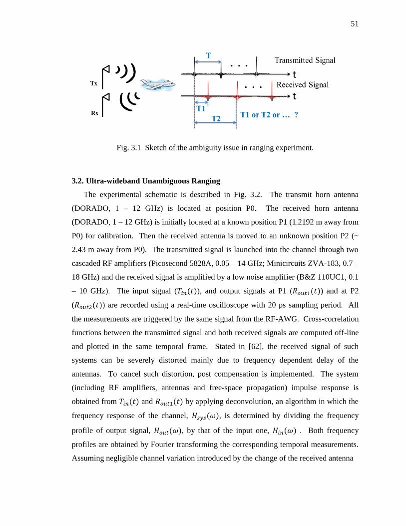
51
Fig. 3.1 Sketch of the ambiguity issue in ranging experiment.
3.2. Ultra-wideband Unambiguous Ranging
The experimental schematic is described in Fig. 3.2. The transmit horn antenna
(DORADO, 1 – 12 GHz) is located at position P0. The received horn antenna
(DORADO, 1 – 12 GHz) is initially located at a known position P1 (1.2192 m away from
P0) for calibration. Then the received antenna is moved to an unknown position P2 (~
2.43 m away from P0). The transmitted signal is launched into the channel through two
cascaded RF amplifiers (Picosecond 5828A, 0.05 – 14 GHz; Minicircuits ZVA-183, 0.7 –
18 GHz) and the received signal is amplified by a low noise amplifier (B&Z 110UC1, 0.1
– 10 GHz). The input signal (𝑇𝑖𝑛(𝑡)), and output signals at P1 (𝑅𝑜𝑢𝑡1(𝑡)) and at P2
(𝑅𝑜𝑢𝑡2(𝑡)) are recorded using a real-time oscilloscope with 20 ps sampling period. All
the measurements are triggered by the same signal from the RF-AWG. Cross-correlation
functions between the transmitted signal and both received signals are computed off-line
and plotted in the same temporal frame. Stated in [62], the received signal of such
systems can be severely distorted mainly due to frequency dependent delay of the
antennas. To cancel such distortion, post compensation is implemented. The system
(including RF amplifiers, antennas and free-space propagation) impulse response is
obtained from 𝑇𝑖𝑛(𝑡) and 𝑅𝑜𝑢𝑡1(𝑡) by applying deconvolution, an algorithm in which the
frequency response of the channel, 𝐻𝑠𝑦𝑠(𝜔), is determined by dividing the frequency
profile of output signal, 𝐻𝑜𝑢𝑡(𝜔), by that of the input one, 𝐻𝑖𝑛(𝜔) . Both frequency
profiles are obtained by Fourier transforming the corresponding temporal measurements.
Assuming negligible channel variation introduced by the change of the received antenna
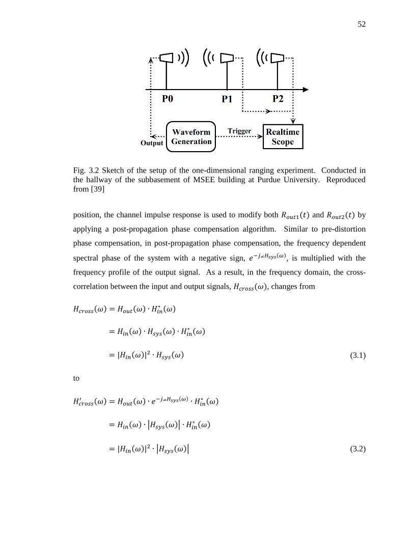
52
Fig. 3.2 Sketch of the setup of the one-dimensional ranging experiment. Conducted in
the hallway of the subbasement of MSEE building at Purdue University. Reproduced
from [39]
position, the channel impulse response is used to modify both 𝑅𝑜𝑢𝑡1(𝑡) and 𝑅𝑜𝑢𝑡2(𝑡) by
applying a post-propagation phase compensation algorithm. Similar to pre-distortion
phase compensation, in post-propagation phase compensation, the frequency dependent
spectral phase of the system with a negative sign, 𝑒−𝑗⦟𝐻𝑠𝑦𝑠(𝜔), is multiplied with the
frequency profile of the output signal. As a result, in the frequency domain, the cross-
correlation between the input and output signals, 𝐻𝑐𝑟𝑜𝑠𝑠(𝜔), changes from
𝐻𝑐𝑟𝑜𝑠𝑠(𝜔) = 𝐻𝑜𝑢𝑡(𝜔) ∙ 𝐻𝑖𝑛∗ (𝜔)
= 𝐻𝑖𝑛(𝜔) ∙ 𝐻𝑠𝑦𝑠(𝜔) ∙ 𝐻𝑖𝑛∗ (𝜔)
= |𝐻𝑖𝑛(𝜔)|2 ∙ 𝐻𝑠𝑦𝑠(𝜔) (3.1)
to
𝐻𝑐𝑟𝑜𝑠𝑠′ (𝜔) = 𝐻𝑜𝑢𝑡(𝜔) ∙ 𝑒
−𝑗⦟𝐻𝑠𝑦𝑠(𝜔) ∙ 𝐻𝑖𝑛∗ (𝜔)
= 𝐻𝑖𝑛(𝜔) ∙ |𝐻𝑠𝑦𝑠(𝜔)| ∙ 𝐻𝑖𝑛∗ (𝜔)
= |𝐻𝑖𝑛(𝜔)|2 ∙ |𝐻𝑠𝑦𝑠(𝜔)| (3.2)
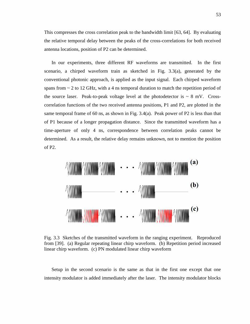
53
This compresses the cross correlation peak to the bandwidth limit [63, 64]. By evaluating
the relative temporal delay between the peaks of the cross-correlations for both received
antenna locations, position of P2 can be determined.
In our experiments, three different RF waveforms are transmitted. In the first
scenario, a chirped waveform train as sketched in Fig. 3.3(a), generated by the
conventional photonic approach, is applied as the input signal. Each chirped waveform
spans from ~ 2 to 12 GHz, with a 4 ns temporal duration to match the repetition period of
the source laser. Peak-to-peak voltage level at the photodetector is ~ 8 mV. Cross-
correlation functions of the two received antenna positions, P1 and P2, are plotted in the
same temporal frame of 60 ns, as shown in Fig. 3.4(a). Peak power of P2 is less than that
of P1 because of a longer propagation distance. Since the transmitted waveform has a
time-aperture of only 4 ns, correspondence between correlation peaks cannot be
determined. As a result, the relative delay remains unknown, not to mention the position
of P2.
Fig. 3.3 Sketches of the transmitted waveform in the ranging experiment. Reproduced
from [39]. (a) Regular repeating linear chirp waveform. (b) Repetition period increased
linear chirp waveform. (c) PN modulated linear chirp waveform
Setup in the second scenario is the same as that in the first one except that one
intensity modulator is added immediately after the laser. The intensity modulator blocks
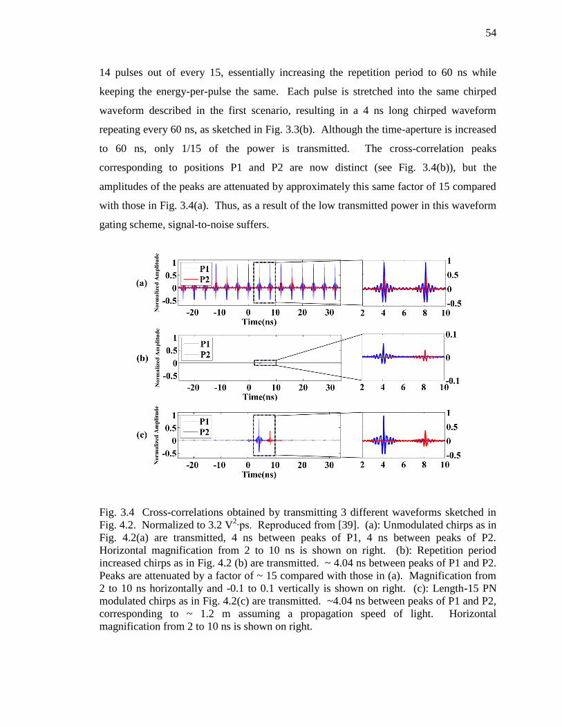
54
14 pulses out of every 15, essentially increasing the repetition period to 60 ns while
keeping the energy-per-pulse the same. Each pulse is stretched into the same chirped
waveform described in the first scenario, resulting in a 4 ns long chirped waveform
repeating every 60 ns, as sketched in Fig. 3.3(b). Although the time-aperture is increased
to 60 ns, only 1/15 of the power is transmitted. The cross-correlation peaks
corresponding to positions P1 and P2 are now distinct (see Fig. 3.4(b)), but the
amplitudes of the peaks are attenuated by approximately this same factor of 15 compared
with those in Fig. 3.4(a). Thus, as a result of the low transmitted power in this waveform
gating scheme, signal-to-noise suffers.
Fig. 3.4 Cross-correlations obtained by transmitting 3 different waveforms sketched in
Fig. 4.2. Normalized to 3.2 V2∙ps. Reproduced from [39]. (a): Unmodulated chirps as in
Fig. 4.2(a) are transmitted, 4 ns between peaks of P1, 4 ns between peaks of P2.
Horizontal magnification from 2 to 10 ns is shown on right. (b): Repetition period
increased chirps as in Fig. 4.2 (b) are transmitted. ~ 4.04 ns between peaks of P1 and P2.
Peaks are attenuated by a factor of ~ 15 compared with those in (a). Magnification from
2 to 10 ns horizontally and -0.1 to 0.1 vertically is shown on right. (c): Length-15 PN
modulated chirps as in Fig. 4.2(c) are transmitted. ~4.04 ns between peaks of P1 and P2,
corresponding to ~ 1.2 m assuming a propagation speed of light. Horizontal
magnification from 2 to 10 ns is shown on right.
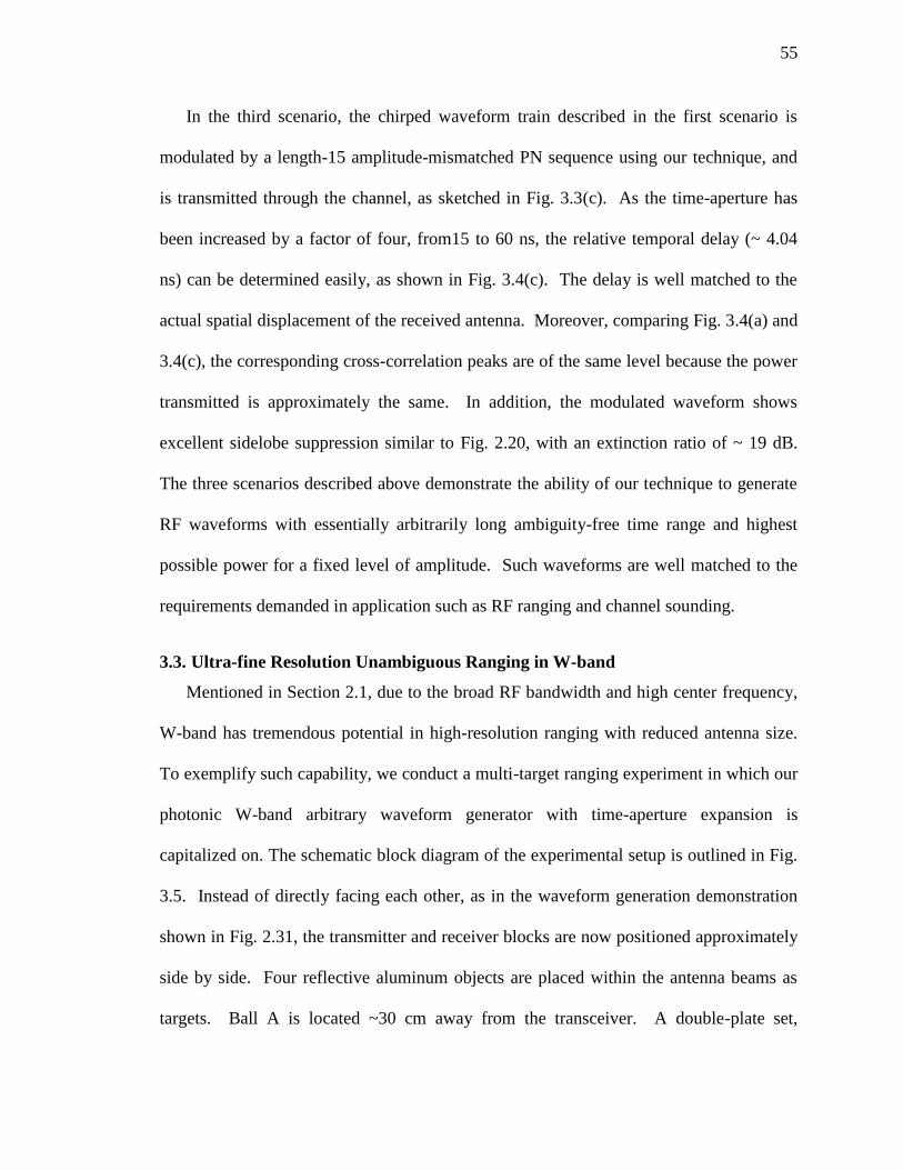
55
In the third scenario, the chirped waveform train described in the first scenario is
modulated by a length-15 amplitude-mismatched PN sequence using our technique, and
is transmitted through the channel, as sketched in Fig. 3.3(c). As the time-aperture has
been increased by a factor of four, from15 to 60 ns, the relative temporal delay (~ 4.04
ns) can be determined easily, as shown in Fig. 3.4(c). The delay is well matched to the
actual spatial displacement of the received antenna. Moreover, comparing Fig. 3.4(a) and
3.4(c), the corresponding cross-correlation peaks are of the same level because the power
transmitted is approximately the same. In addition, the modulated waveform shows
excellent sidelobe suppression similar to Fig. 2.20, with an extinction ratio of ~ 19 dB.
The three scenarios described above demonstrate the ability of our technique to generate
RF waveforms with essentially arbitrarily long ambiguity-free time range and highest
possible power for a fixed level of amplitude. Such waveforms are well matched to the
requirements demanded in application such as RF ranging and channel sounding.
3.3. Ultra-fine Resolution Unambiguous Ranging in W-band
Mentioned in Section 2.1, due to the broad RF bandwidth and high center frequency,
W-band has tremendous potential in high-resolution ranging with reduced antenna size.
To exemplify such capability, we conduct a multi-target ranging experiment in which our
photonic W-band arbitrary waveform generator with time-aperture expansion is
capitalized on. The schematic block diagram of the experimental setup is outlined in Fig.
3.5. Instead of directly facing each other, as in the waveform generation demonstration
shown in Fig. 2.31, the transmitter and receiver blocks are now positioned approximately
side by side. Four reflective aluminum objects are placed within the antenna beams as
targets. Ball A is located ~30 cm away from the transceiver. A double-plate set,
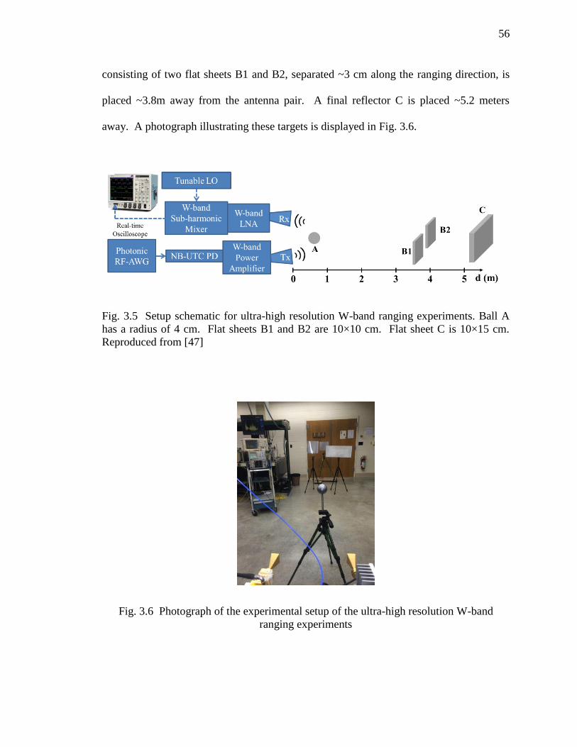
56
consisting of two flat sheets B1 and B2, separated ~3 cm along the ranging direction, is
placed ~3.8m away from the antenna pair. A final reflector C is placed ~5.2 meters
away. A photograph illustrating these targets is displayed in Fig. 3.6.
Fig. 3.5 Setup schematic for ultra-high resolution W-band ranging experiments. Ball A
has a radius of 4 cm. Flat sheets B1 and B2 are 10×10 cm. Flat sheet C is 10×15 cm.
Reproduced from [47]
Fig. 3.6 Photograph of the experimental setup of the ultra-high resolution W-band
ranging experiments
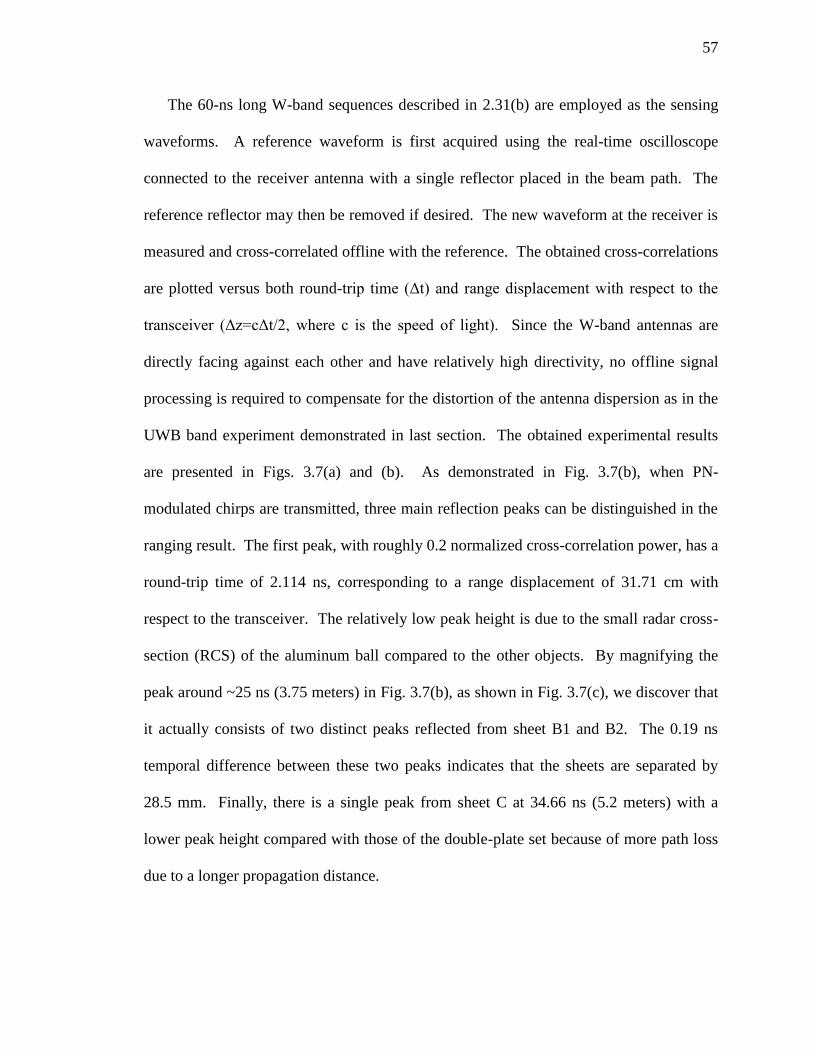
57
The 60-ns long W-band sequences described in 2.31(b) are employed as the sensing
waveforms. A reference waveform is first acquired using the real-time oscilloscope
connected to the receiver antenna with a single reflector placed in the beam path. The
reference reflector may then be removed if desired. The new waveform at the receiver is
measured and cross-correlated offline with the reference. The obtained cross-correlations
are plotted versus both round-trip time (Δt) and range displacement with respect to the
transceiver (Δz=cΔt/2, where c is the speed of light). Since the W-band antennas are
directly facing against each other and have relatively high directivity, no offline signal
processing is required to compensate for the distortion of the antenna dispersion as in the
UWB band experiment demonstrated in last section. The obtained experimental results
are presented in Figs. 3.7(a) and (b). As demonstrated in Fig. 3.7(b), when PN-
modulated chirps are transmitted, three main reflection peaks can be distinguished in the
ranging result. The first peak, with roughly 0.2 normalized cross-correlation power, has a
round-trip time of 2.114 ns, corresponding to a range displacement of 31.71 cm with
respect to the transceiver. The relatively low peak height is due to the small radar cross-
section (RCS) of the aluminum ball compared to the other objects. By magnifying the
peak around ~25 ns (3.75 meters) in Fig. 3.7(b), as shown in Fig. 3.7(c), we discover that
it actually consists of two distinct peaks reflected from sheet B1 and B2. The 0.19 ns
temporal difference between these two peaks indicates that the sheets are separated by
28.5 mm. Finally, there is a single peak from sheet C at 34.66 ns (5.2 meters) with a
lower peak height compared with those of the double-plate set because of more path loss
due to a longer propagation distance.
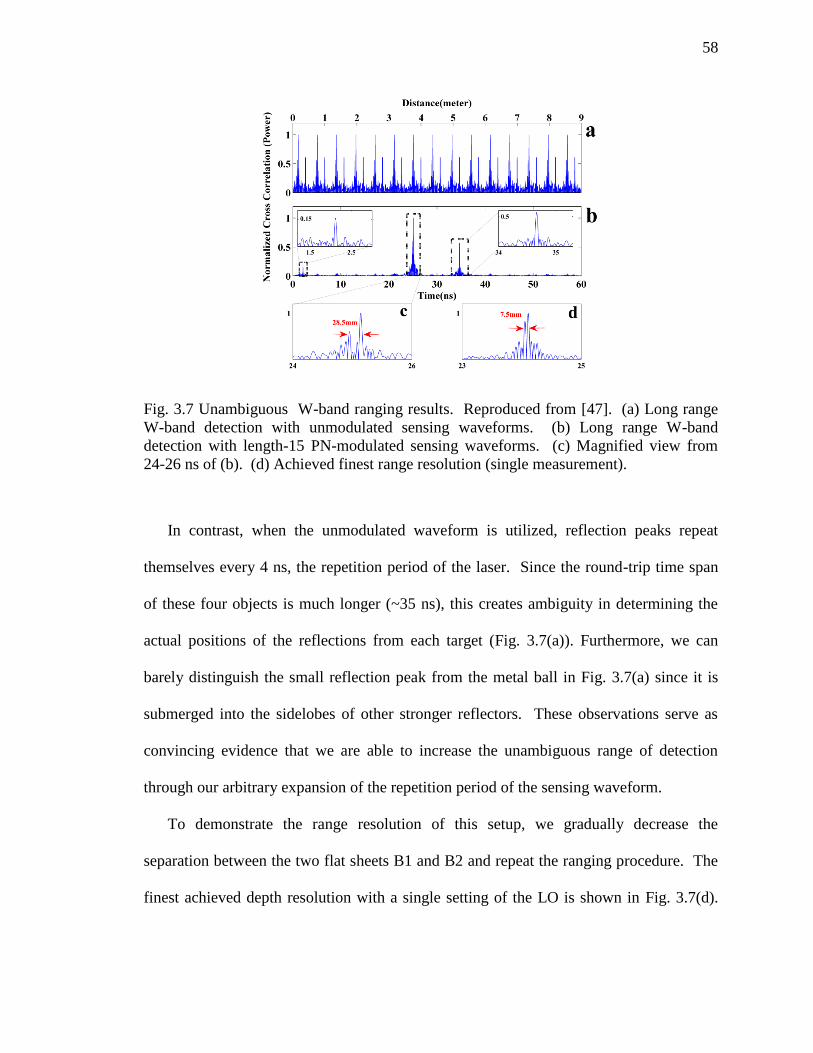
58
Fig. 3.7 Unambiguous W-band ranging results. Reproduced from [47]. (a) Long range
W-band detection with unmodulated sensing waveforms. (b) Long range W-band
detection with length-15 PN-modulated sensing waveforms. (c) Magnified view from
24-26 ns of (b). (d) Achieved finest range resolution (single measurement).
In contrast, when the unmodulated waveform is utilized, reflection peaks repeat
themselves every 4 ns, the repetition period of the laser. Since the round-trip time span
of these four objects is much longer (~35 ns), this creates ambiguity in determining the
actual positions of the reflections from each target (Fig. 3.7(a)). Furthermore, we can
barely distinguish the small reflection peak from the metal ball in Fig. 3.7(a) since it is
submerged into the sidelobes of other stronger reflectors. These observations serve as
convincing evidence that we are able to increase the unambiguous range of detection
through our arbitrary expansion of the repetition period of the sensing waveform.
To demonstrate the range resolution of this setup, we gradually decrease the
separation between the two flat sheets B1 and B2 and repeat the ranging procedure. The
finest achieved depth resolution with a single setting of the LO is shown in Fig. 3.7(d).
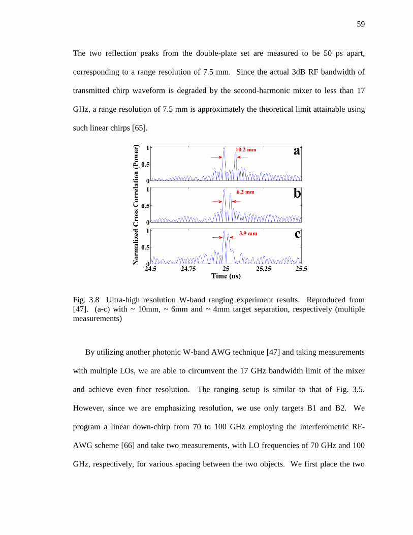
59
The two reflection peaks from the double-plate set are measured to be 50 ps apart,
corresponding to a range resolution of 7.5 mm. Since the actual 3dB RF bandwidth of
transmitted chirp waveform is degraded by the second-harmonic mixer to less than 17
GHz, a range resolution of 7.5 mm is approximately the theoretical limit attainable using
such linear chirps [65].
Fig. 3.8 Ultra-high resolution W-band ranging experiment results. Reproduced from
[47]. (a-c) with ~ 10mm, ~ 6mm and ~ 4mm target separation, respectively (multiple
measurements)
By utilizing another photonic W-band AWG technique [47] and taking measurements
with multiple LOs, we are able to circumvent the 17 GHz bandwidth limit of the mixer
and achieve even finer resolution. The ranging setup is similar to that of Fig. 3.5.
However, since we are emphasizing resolution, we use only targets B1 and B2. We
program a linear down-chirp from 70 to 100 GHz employing the interferometric RF-
AWG scheme [66] and take two measurements, with LO frequencies of 70 GHz and 100
GHz, respectively, for various spacing between the two objects. We first place the two
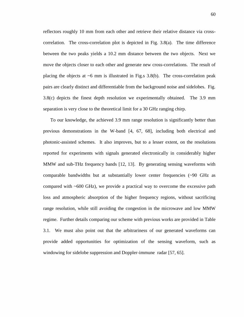
60
reflectors roughly 10 mm from each other and retrieve their relative distance via cross-
correlation. The cross-correlation plot is depicted in Fig. 3.8(a). The time difference
between the two peaks yields a 10.2 mm distance between the two objects. Next we
move the objects closer to each other and generate new cross-correlations. The result of
placing the objects at ~6 mm is illustrated in Fig.s 3.8(b). The cross-correlation peak
pairs are clearly distinct and differentiable from the background noise and sidelobes. Fig.
3.8(c) depicts the finest depth resolution we experimentally obtained. The 3.9 mm
separation is very close to the theoretical limit for a 30 GHz ranging chirp.
To our knowledge, the achieved 3.9 mm range resolution is significantly better than
previous demonstrations in the W-band [4, 67, 68], including both electrical and
photonic-assisted schemes. It also improves, but to a lesser extent, on the resolutions
reported for experiments with signals generated electronically in considerably higher
MMW and sub-THz frequency bands [12, 13]. By generating sensing waveforms with
comparable bandwidths but at substantially lower center frequencies (~90 GHz as
compared with ~600 GHz), we provide a practical way to overcome the excessive path
loss and atmospheric absorption of the higher frequency regions, without sacrificing
range resolution, while still avoiding the congestion in the microwave and low MMW
regime. Further details comparing our scheme with previous works are provided in Table
3.1. We must also point out that the arbitrariness of our generated waveforms can
provide added opportunities for optimization of the sensing waveform, such as
windowing for sidelobe suppression and Doppler-immune radar [57, 65].
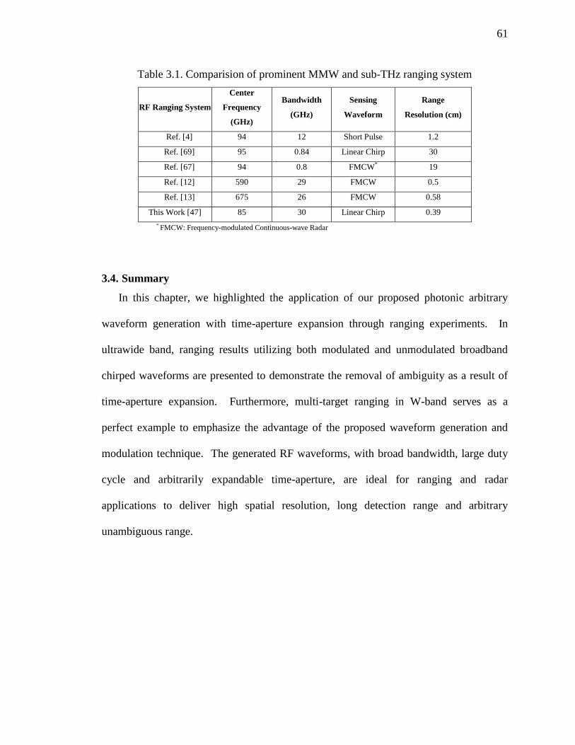
61
Table 3.1. Comparision of prominent MMW and sub-THz ranging system
RF Ranging System
Center
Frequency
(GHz)
Bandwidth
(GHz)
Sensing
Waveform
Range
Resolution (cm)
Ref. [4] 94 12 Short Pulse 1.2
Ref. [69] 95 0.84 Linear Chirp 30
Ref. [67] 94 0.8 FMCW* 19
Ref. [12] 590 29 FMCW 0.5
Ref. [13] 675 26 FMCW 0.58
This Work [47] 85 30 Linear Chirp 0.39
* FMCW: Frequency-modulated Continuous-wave Radar
3.4. Summary
In this chapter, we highlighted the application of our proposed photonic arbitrary
waveform generation with time-aperture expansion through ranging experiments. In
ultrawide band, ranging results utilizing both modulated and unmodulated broadband
chirped waveforms are presented to demonstrate the removal of ambiguity as a result of
time-aperture expansion. Furthermore, multi-target ranging in W-band serves as a
perfect example to emphasize the advantage of the proposed waveform generation and
modulation technique. The generated RF waveforms, with broad bandwidth, large duty
cycle and arbitrarily expandable time-aperture, are ideal for ranging and radar
applications to deliver high spatial resolution, long detection range and arbitrary
unambiguous range.
62
4. ULTRA WIDEBAND WIRELESS COMMUNICATION
4.1. Background
The tremendous potentials in delivering ultra-high speed data transmission have
motivated researches to explore the wideband wireless communication system. The
primary advantage of wideband communication, compared with narrowband
communication, is the higher achievable data rate determined by Shannon-Hartley
theorem. In addition, broadband systems have potentially low complexity and low cost,
which arises from the baseband nature of the signal transmission [3]. Unlike in the
common case of narrowband communication systems, the transmitter in broadband
communication systems generates waveforms without an additional RF mixing stage to
up-convert the baseband signal to a frequency with desirable propagation characteristics.
Consequently, down-conversion at the receiver and local oscillators as well as complex
delay and phase tracking loops on both ends of the transmission system are not required
anymore. Such high-data rate and low cost properties present a unique opportunity for
wideband communication to impact the way of wireless data transmission.
However, there are still a large number of problems that have to be overcome before
wideband communication systems can be introduced for practical application. We have
addressed the difficulties in terms of waveform generation and signal distribution in
previous chapters to prove that photonics is the most promising approach for wideband
communications. In fact, there have been extensive studies in signal synthesis and
63
wireless data transmission in the 3.1-10.6 GHz frequency range. Refs. [70-73] have
demonstrated the use of photonics for data generation and wired optical fiber distribution
of UWB signals, together with free space transmission over simple wireless channels.
However, a broadband input signal, after propagating through the wireless channel, will
experience frequency-dependent distortions, primarily due to the dispersion of the
antennas and other components, as well as the frequency-dependent reflection and
refraction of the propagation environment. More importantly, in an indoor environment,
where a wideband wireless communication system will most likely be deployed, the
transmitted signal arrives at the receiver through different paths, as illustrated in Fig. 4.1.
Consequently, these delayed and distorted versions of the transmitted signal may add up
at the receiver constructively or destructively, further increasing the signal distortions. A
transmitted short pulse is often distorted into a very complex waveform with long delay
spread. Without proper compensation, the aforementioned distortions can severely
degrade the performance of the communication system through intersymbol interference
(ISI). What makes the situation even worse is, as the center frequency of the wireless
system scales up, the spatial coherence drops down. In another word, the distortion
experienced by a transmitted signal becomes almost completely de-correlated even with a
few centimeters of antenna displacement. All of the above-mentioned issues require the
wideband communication system to have a functionality of programmable distortion
compensation, perhaps with decent update speed for mobile channel, in order to mitigate
the ISI introduced by dispersion and multipath. It is also worth noticing that, distortion
compensation can be performed in either side of the signal transmission. At the receiver
side, RF filters or digital signal processing can be employed to compress the received
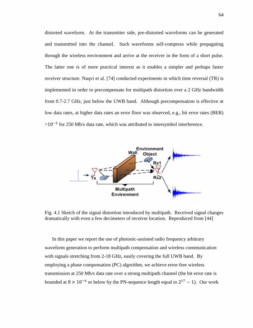
64
distorted waveform. At the transmitter side, pre-distorted waveforms can be generated
and transmitted into the channel. Such waveforms self-compress while propagating
through the wireless environment and arrive at the receiver in the form of a short pulse.
The latter one is of more practical interest as it enables a simpler and perhaps faster
receiver structure. Naqvi et al. [74] conducted experiments in which time reversal (TR) is
implemented in order to precompensate for multipath distortion over a 2 GHz bandwidth
from 0.7-2.7 GHz, just below the UWB band. Although precompensation is effective at
low data rates, at higher data rates an error floor was observed, e.g., bit error rates (BER)
>10−2 for 250 Mb/s data rate, which was attributed to intersymbol interference.
Fig. 4.1 Sketch of the signal distortion introduced by multipath. Received signal changes
dramatically with even a few decimeters of receiver location. Reproduced from [44]
In this paper we report the use of photonic-assisted radio frequency arbitrary
waveform generation to perform multipath compensation and wireless communication
with signals stretching from 2-18 GHz, easily covering the full UWB band. By
employing a phase compensation (PC) algorithm, we achieve error-free wireless
transmission at 250 Mb/s data rate over a strong multipath channel (the bit error rate is
bounded at 8 × 10⁻⁶ or below by the PN-sequence length equal to 217 − 1). Our work
65
which is the first to compare the performance of TR and PC directly in communications
experiments, confirms the prediction [64] that phase compensation provides substantial
superiority over time reversal in terms of ISI suppression.
4.2. Spread Spectrum Channel Sounding
The very first step in achieving broadband wireless communication with distortion
suppression is channel sounding. Channel sounding is the process in which the
information of the signal propagation environment (may include amplifiers, filters,
antennas and free-space environment) is obtained, normally in the form of channel
impulse response and frequency response. Such information is essential in the later stage
of distortion compensation. A commonly used frequency-domain instrument for channel
sounding is the vector network analyzer (VNA) [2]. A VNA generates a narrowband
probing signal and measures the corresponding response of the device-under-test (DUT).
By sweeping across the frequency range of interest, both amplitude and phase
information can be retrieved after further digital signal processing. A VNA, while
providing fine frequency resolution, is essentially a discrete and time-consuming
technique, especially when employed to investigate ultra broad bandwidth. Another
category of channel sounding method is based on temporal domain techniques. Example
is the short-pulse excitation [75]. Short RF pulse, with bandwidth wide enough to cover
the whole frequency range of interest, is transmitted to excite the channel. In this way,
the received waveform at the output of the system, measured by oscilloscope, is the
impulse response of the channel with approximation. Clearly, this technique offers much
faster channel sounding speed and thus desirable in the characterization of broadband
channels. However, as most components and devices are peak-voltage-limited,
66
analogous to pulsed-radar, short pulse does not provide enough transmitted power to
overcome the severe attenuation of the propagation environment, especially at higher
frequencies. Consequently, spread spectrum channel sounding has gained popularity
over the years. In this approach, spread spectrum waveforms, characterized by broad RF
bandwidth and high average transmitted power due to long time-apertures, are
transmitted to excite the channel [76, 77]. Both transmitted and received waveforms are
measured by an oscilloscope and used in offline digital signal processing, in which
algorithms like cross-correlation or deconvolution can be applied to retrieve the impulse
response as well as the frequency response of the excited channel. An example of a
spread spectrum waveform is the frequency sweeping (chirped) waveform, whose
instantaneous frequency changes linearly with time.
Spread spectrum waveforms for channel sounding must be evaluated in three aspects:
RF bandwidth, time-aperture and repetition period. The RF bandwidth of the sounding
waveform should cover the full frequency range of interest to resolve the finest features
in the impulse response of the channel. In the peak-voltage-limited scenario, the time-
aperture of the waveform directly determines the average power in the peak-voltage-
limited scenario and thus should be engineered as long as possible. From time domain
point of view, the repetition period of the sounding waveform must exceed the delay
spread of the channel to remove the ambiguity when consecutive received waveforms
overlap in time. From a frequency domain point of view, the repetition period is
inversely proportional to the frequency resolution of the sounding waveform. In this
regard, the repetition period of the sounding waveform should be set long enough to
resolve the finest features in the frequency response of the channel. Based on the above
67
analyses, photonically generated linear chirped waveforms with pseudorandom sequence
modulation introduced in Chapter 2 are the perfect candidates for ultra broadband
channel sounding purpose. They cover a broad range of frequency with 100% duty cycle,
essentially the maximum achievable average power in peak-voltage-limited case. More
importantly, the repetition period of the waveform can be arbitrarily expanded to safely
ensure that all features in the frequency response of the channel can be adequately
resolved.
The procedure of ultra broadband channel sounding is as follow:
1. A spread spectrum chirped waveform with 4 ns time aperture and 4 ns repetition
period is photonically generated. The RF bandwidth and the PN modulation are
determined by the requirements of the specific experiment. The time domain
measurement of the generated waveform, denoted ℎ𝑖𝑛(𝑡) is recorded by a real-time
oscilloscope with a sampling period of 20 ps.
2. The generated waveform is transmitted into the system, which may include RF
amplifiers, filters, antennas and the free space propagation environment. The output
signal at the receiver, denoted ℎ𝑜𝑢𝑡(𝑡) is also measured by the real-time oscilloscope with
the same sampling window.
3. The Fourier transform of both the input and output signals is performed offline in a
computer, generating the input and output spectrum, 𝐻𝑖𝑛(𝑓) and 𝐻𝑜𝑢𝑡(𝑓), respectively.
4. A deconvolution algorithm is applied in which the frequency response of the
system, 𝐻𝑠𝑦𝑠(𝑓), is determined by
𝐻𝑠𝑦𝑠(𝑓) =𝐻𝑜𝑢𝑡(𝑓)
𝐻𝑖𝑛(𝑓)
(4.1)
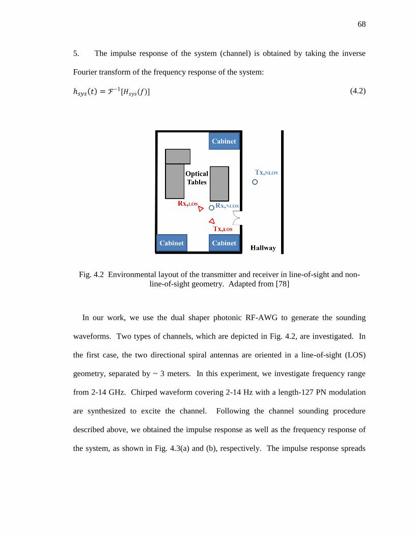
68
5. The impulse response of the system (channel) is obtained by taking the inverse
Fourier transform of the frequency response of the system:
ℎ𝑠𝑦𝑠(𝑡) = ℱ−1[𝐻𝑠𝑦𝑠(𝑓)] (4.2)
Fig. 4.2 Environmental layout of the transmitter and receiver in line-of-sight and non-
line-of-sight geometry. Adapted from [78]
In our work, we use the dual shaper photonic RF-AWG to generate the sounding
waveforms. Two types of channels, which are depicted in Fig. 4.2, are investigated. In
the first case, the two directional spiral antennas are oriented in a line-of-sight (LOS)
geometry, separated by ~ 3 meters. In this experiment, we investigate frequency range
from 2-14 GHz. Chirped waveform covering 2-14 Hz with a length-127 PN modulation
are synthesized to excite the channel. Following the channel sounding procedure
described above, we obtained the impulse response as well as the frequency response of
the system, as shown in Fig. 4.3(a) and (b), respectively. The impulse response spreads
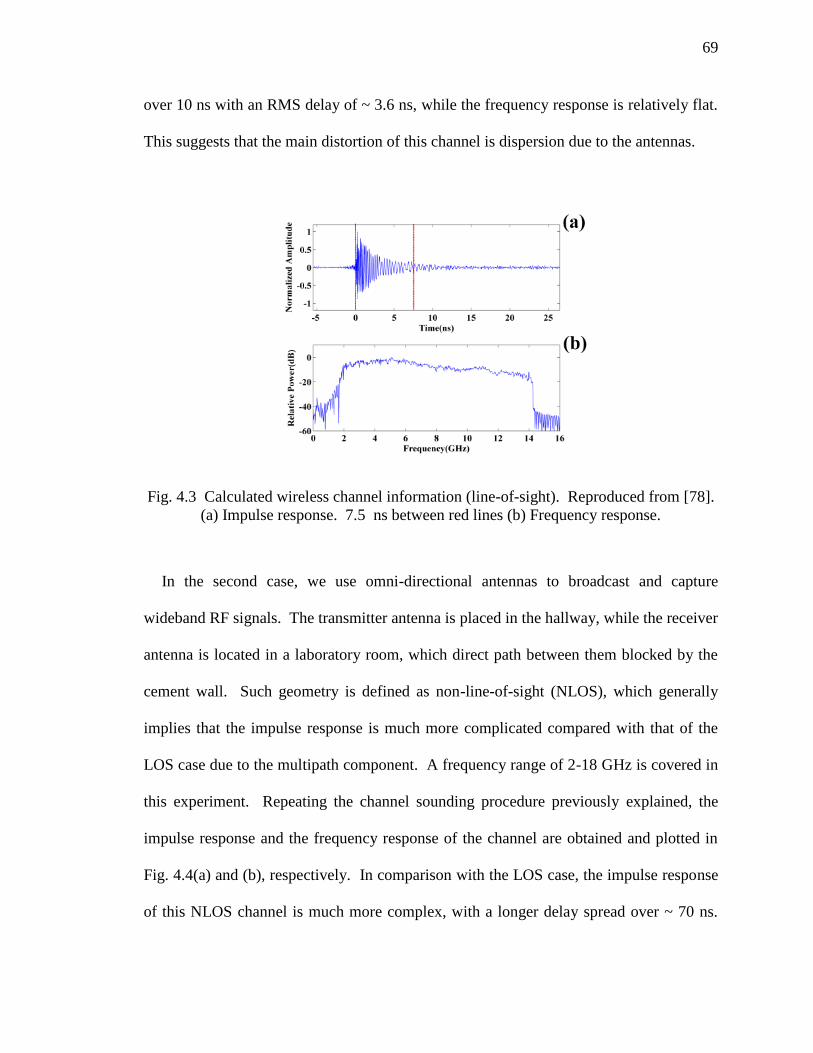
69
over 10 ns with an RMS delay of ~ 3.6 ns, while the frequency response is relatively flat.
This suggests that the main distortion of this channel is dispersion due to the antennas.
Fig. 4.3 Calculated wireless channel information (line-of-sight). Reproduced from [78].
(a) Impulse response. 7.5 ns between red lines (b) Frequency response.
In the second case, we use omni-directional antennas to broadcast and capture
wideband RF signals. The transmitter antenna is placed in the hallway, while the receiver
antenna is located in a laboratory room, which direct path between them blocked by the
cement wall. Such geometry is defined as non-line-of-sight (NLOS), which generally
implies that the impulse response is much more complicated compared with that of the
LOS case due to the multipath component. A frequency range of 2-18 GHz is covered in
this experiment. Repeating the channel sounding procedure previously explained, the
impulse response and the frequency response of the channel are obtained and plotted in
Fig. 4.4(a) and (b), respectively. In comparison with the LOS case, the impulse response
of this NLOS channel is much more complex, with a longer delay spread over ~ 70 ns.
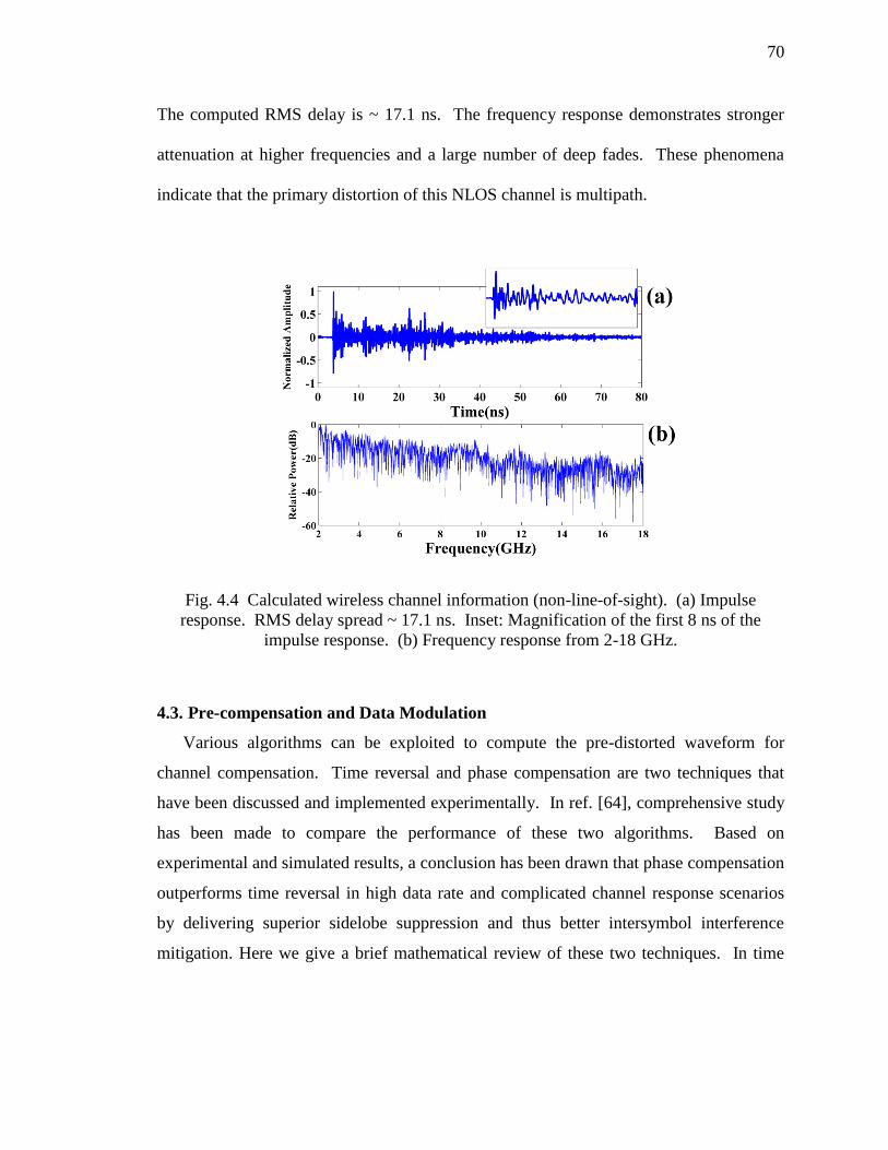
70
The computed RMS delay is ~ 17.1 ns. The frequency response demonstrates stronger
attenuation at higher frequencies and a large number of deep fades. These phenomena
indicate that the primary distortion of this NLOS channel is multipath.
Fig. 4.4 Calculated wireless channel information (non-line-of-sight). (a) Impulse
response. RMS delay spread ~ 17.1 ns. Inset: Magnification of the first 8 ns of the
impulse response. (b) Frequency response from 2-18 GHz.
4.3. Pre-compensation and Data Modulation
Various algorithms can be exploited to compute the pre-distorted waveform for
channel compensation. Time reversal and phase compensation are two techniques that
have been discussed and implemented experimentally. In ref. [64], comprehensive study
has been made to compare the performance of these two algorithms. Based on
experimental and simulated results, a conclusion has been drawn that phase compensation
outperforms time reversal in high data rate and complicated channel response scenarios
by delivering superior sidelobe suppression and thus better intersymbol interference
mitigation. Here we give a brief mathematical review of these two techniques. In time
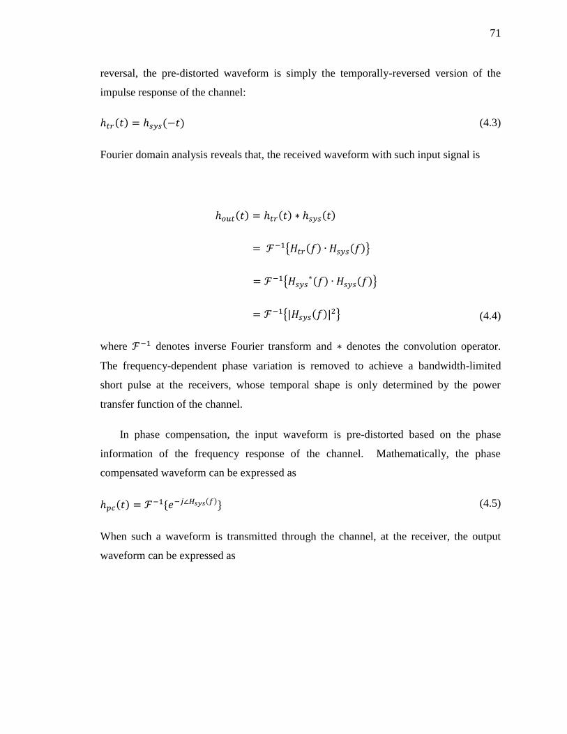
71
reversal, the pre-distorted waveform is simply the temporally-reversed version of the
impulse response of the channel:
ℎ𝑡𝑟(𝑡) = ℎ𝑠𝑦𝑠(−𝑡) (4.3)
Fourier domain analysis reveals that, the received waveform with such input signal is
ℎ𝑜𝑢𝑡(𝑡) = ℎ𝑡𝑟(𝑡) ∗ ℎ𝑠𝑦𝑠(𝑡)
= ℱ−1{𝐻𝑡𝑟(𝑓) ∙ 𝐻𝑠𝑦𝑠(𝑓)}
= ℱ−1{𝐻𝑠𝑦𝑠∗(𝑓) ∙ 𝐻𝑠𝑦𝑠(𝑓)}
= ℱ−1{|𝐻𝑠𝑦𝑠(𝑓)|2} (4.4)
where ℱ−1 denotes inverse Fourier transform and ∗ denotes the convolution operator.
The frequency-dependent phase variation is removed to achieve a bandwidth-limited
short pulse at the receivers, whose temporal shape is only determined by the power
transfer function of the channel.
In phase compensation, the input waveform is pre-distorted based on the phase
information of the frequency response of the channel. Mathematically, the phase
compensated waveform can be expressed as
ℎ𝑝𝑐(𝑡) = ℱ−1{𝑒−𝑗∠𝐻𝑠𝑦𝑠(𝑓)} (4.5)
When such a waveform is transmitted through the channel, at the receiver, the output
waveform can be expressed as
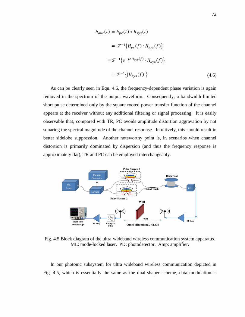
72
ℎ𝑜𝑢𝑡(𝑡) = ℎ𝑝𝑐(𝑡) ∗ ℎ𝑠𝑦𝑠(𝑡)
= ℱ−1{𝐻𝑝𝑐(𝑓) ∙ 𝐻𝑠𝑦𝑠(𝑓)}
= ℱ−1{𝑒−𝑗∠𝐻𝑠𝑦𝑠(𝑓) ∙ 𝐻𝑠𝑦𝑠(𝑓)}
= ℱ−1{|𝐻𝑠𝑦𝑠(𝑓)|} (4.6)
As can be clearly seen in Equ. 4.6, the frequency-dependent phase variation is again
removed in the spectrum of the output waveform. Consequently, a bandwidth-limited
short pulse determined only by the square rooted power transfer function of the channel
appears at the receiver without any additional filtering or signal processing. It is easily
observable that, compared with TR, PC avoids amplitude distortion aggravation by not
squaring the spectral magnitude of the channel response. Intuitively, this should result in
better sidelobe suppression. Another noteworthy point is, in scenarios when channel
distortion is primarily dominated by dispersion (and thus the frequency response is
approximately flat), TR and PC can be employed interchangeably.
Fig. 4.5 Block diagram of the ultra-wideband wireless communication system apparatus.
ML: mode-locked laser. PD: photodetector. Amp: amplifier.
In our photonic subsystem for ultra wideband wireless communication depicted in
Fig. 4.5, which is essentially the same as the dual-shaper scheme, data modulation is
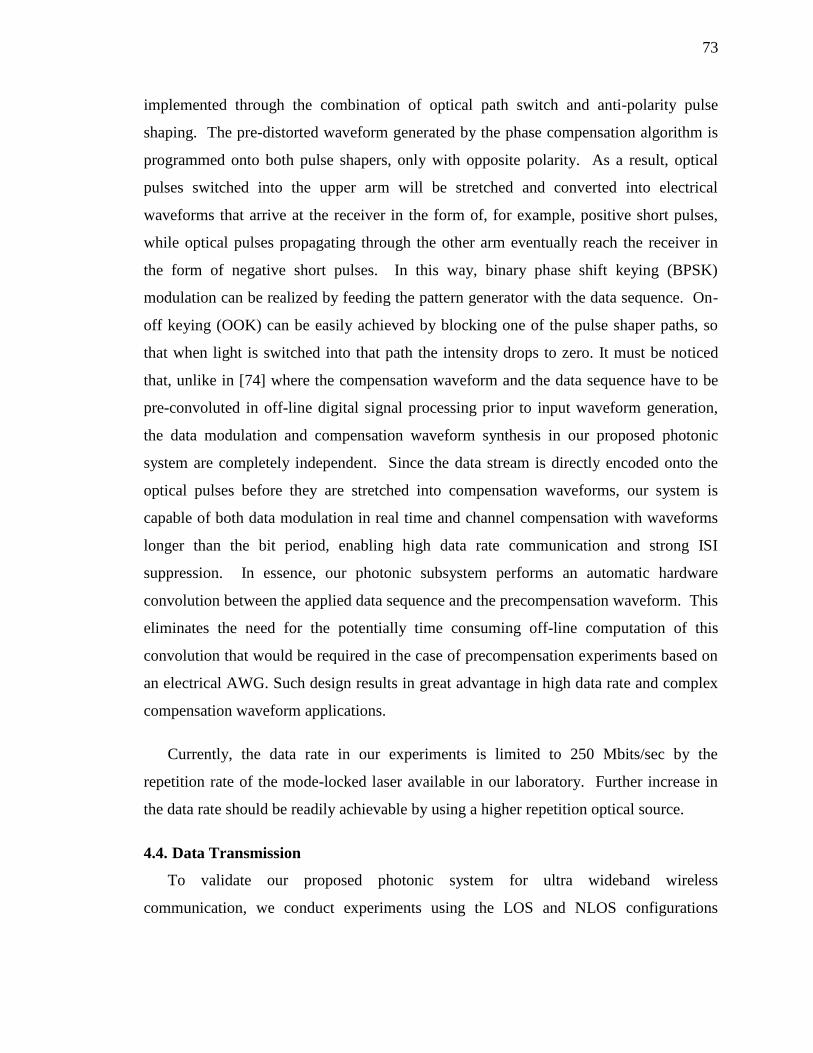
73
implemented through the combination of optical path switch and anti-polarity pulse
shaping. The pre-distorted waveform generated by the phase compensation algorithm is
programmed onto both pulse shapers, only with opposite polarity. As a result, optical
pulses switched into the upper arm will be stretched and converted into electrical
waveforms that arrive at the receiver in the form of, for example, positive short pulses,
while optical pulses propagating through the other arm eventually reach the receiver in
the form of negative short pulses. In this way, binary phase shift keying (BPSK)
modulation can be realized by feeding the pattern generator with the data sequence. On-
off keying (OOK) can be easily achieved by blocking one of the pulse shaper paths, so
that when light is switched into that path the intensity drops to zero. It must be noticed
that, unlike in [74] where the compensation waveform and the data sequence have to be
pre-convoluted in off-line digital signal processing prior to input waveform generation,
the data modulation and compensation waveform synthesis in our proposed photonic
system are completely independent. Since the data stream is directly encoded onto the
optical pulses before they are stretched into compensation waveforms, our system is
capable of both data modulation in real time and channel compensation with waveforms
longer than the bit period, enabling high data rate communication and strong ISI
suppression. In essence, our photonic subsystem performs an automatic hardware
convolution between the applied data sequence and the precompensation waveform. This
eliminates the need for the potentially time consuming off-line computation of this
convolution that would be required in the case of precompensation experiments based on
an electrical AWG. Such design results in great advantage in high data rate and complex
compensation waveform applications.
Currently, the data rate in our experiments is limited to 250 Mbits/sec by the
repetition rate of the mode-locked laser available in our laboratory. Further increase in
the data rate should be readily achievable by using a higher repetition optical source.
4.4. Data Transmission
To validate our proposed photonic system for ultra wideband wireless
communication, we conduct experiments using the LOS and NLOS configurations
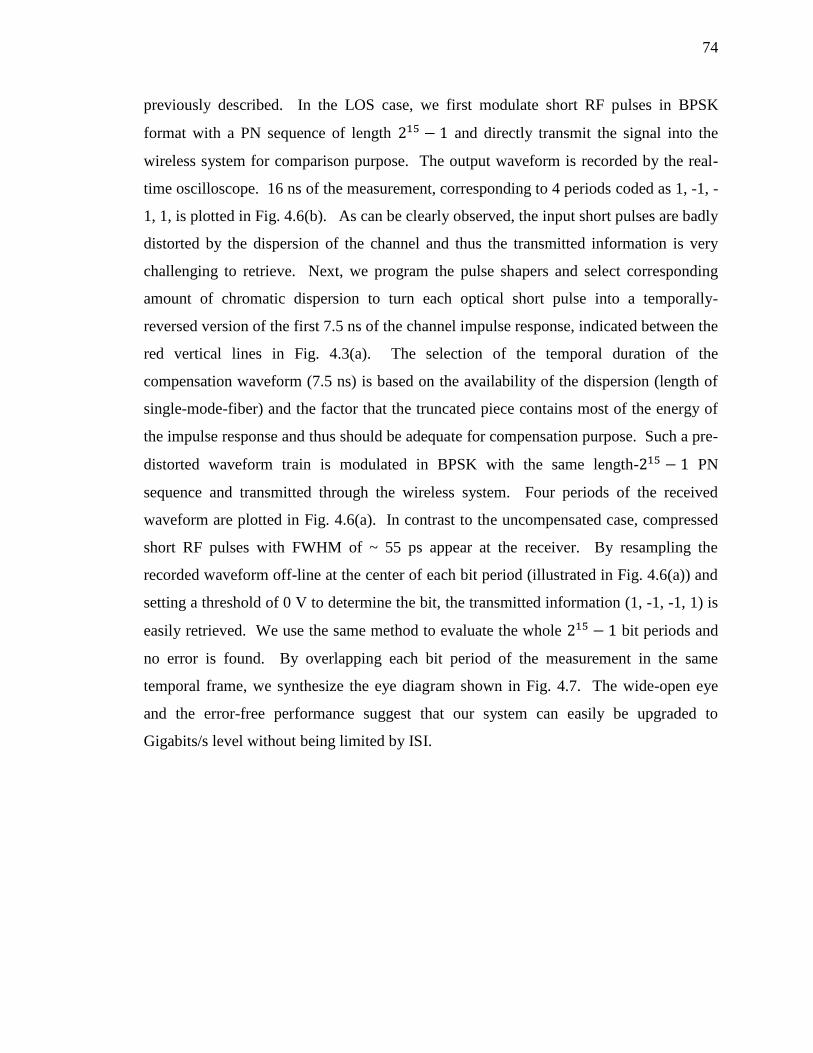
74
previously described. In the LOS case, we first modulate short RF pulses in BPSK
format with a PN sequence of length 215 − 1 and directly transmit the signal into the
wireless system for comparison purpose. The output waveform is recorded by the real-
time oscilloscope. 16 ns of the measurement, corresponding to 4 periods coded as 1, -1, -
1, 1, is plotted in Fig. 4.6(b). As can be clearly observed, the input short pulses are badly
distorted by the dispersion of the channel and thus the transmitted information is very
challenging to retrieve. Next, we program the pulse shapers and select corresponding
amount of chromatic dispersion to turn each optical short pulse into a temporally-
reversed version of the first 7.5 ns of the channel impulse response, indicated between the
red vertical lines in Fig. 4.3(a). The selection of the temporal duration of the
compensation waveform (7.5 ns) is based on the availability of the dispersion (length of
single-mode-fiber) and the factor that the truncated piece contains most of the energy of
the impulse response and thus should be adequate for compensation purpose. Such a pre-
distorted waveform train is modulated in BPSK with the same length-215 − 1 PN
sequence and transmitted through the wireless system. Four periods of the received
waveform are plotted in Fig. 4.6(a). In contrast to the uncompensated case, compressed
short RF pulses with FWHM of ~ 55 ps appear at the receiver. By resampling the
recorded waveform off-line at the center of each bit period (illustrated in Fig. 4.6(a)) and
setting a threshold of 0 V to determine the bit, the transmitted information (1, -1, -1, 1) is
easily retrieved. We use the same method to evaluate the whole 215 − 1 bit periods and
no error is found. By overlapping each bit period of the measurement in the same
temporal frame, we synthesize the eye diagram shown in Fig. 4.7. The wide-open eye
and the error-free performance suggest that our system can easily be upgraded to
Gigabits/s level without being limited by ISI.
75
Fig. 4.6 Received signals with BPSK data modulation (line-of-sight). (a) With 7.5 ns
pre-distorted waveform as input. Red dots indicate the sampling position for BER
calculation. (b) With short pulse inputs
Fig. 4.7 Eye diagram of the received signal corresponding to the situation of Fig. 4.6(a).
In the NLOS case, for comparison, we first transmit an on-off-keyed sequence of
short RF pulses directly generated from the laser through O/E conversion into the
wireless system. In this experiment on-off keying is achieved by blocking one of the
pulse shaper paths, so that when light is switched into that path the intensity drops to
zero. The output waveform is recorded by the real-time oscilloscope, and 16 ns of the
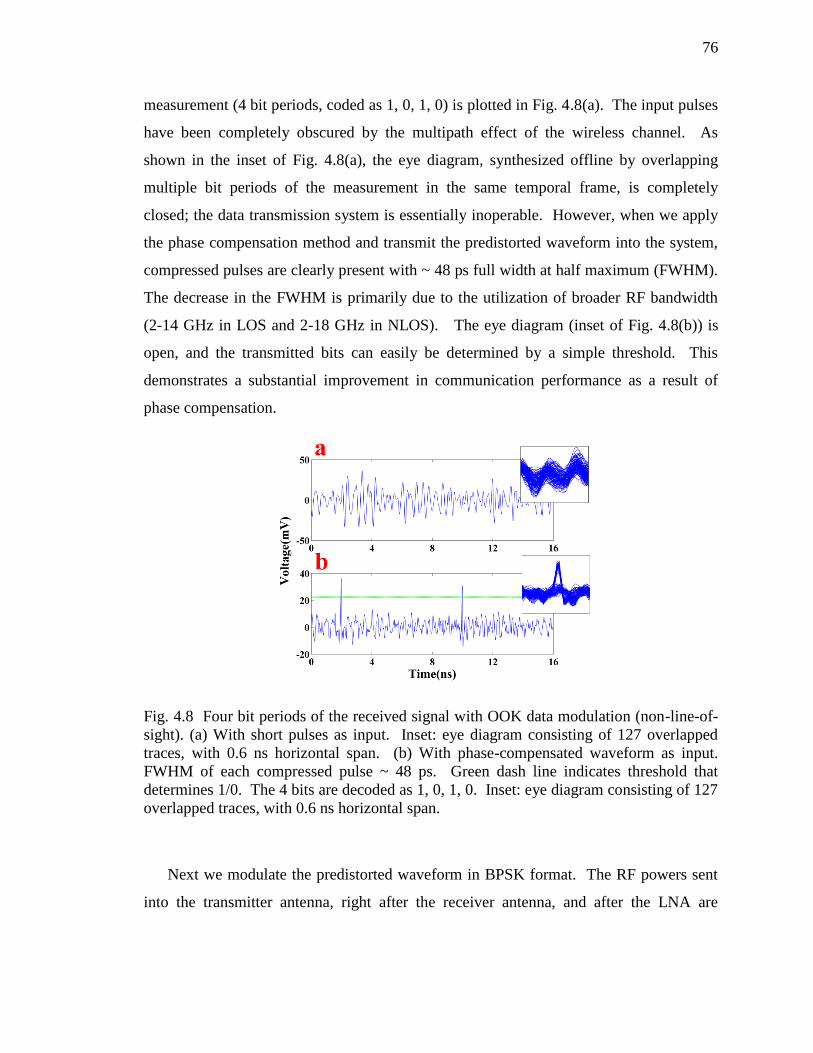
76
measurement (4 bit periods, coded as 1, 0, 1, 0) is plotted in Fig. 4.8(a). The input pulses
have been completely obscured by the multipath effect of the wireless channel. As
shown in the inset of Fig. 4.8(a), the eye diagram, synthesized offline by overlapping
multiple bit periods of the measurement in the same temporal frame, is completely
closed; the data transmission system is essentially inoperable. However, when we apply
the phase compensation method and transmit the predistorted waveform into the system,
compressed pulses are clearly present with ~ 48 ps full width at half maximum (FWHM).
The decrease in the FWHM is primarily due to the utilization of broader RF bandwidth
(2-14 GHz in LOS and 2-18 GHz in NLOS). The eye diagram (inset of Fig. 4.8(b)) is
open, and the transmitted bits can easily be determined by a simple threshold. This
demonstrates a substantial improvement in communication performance as a result of
phase compensation.
Fig. 4.8 Four bit periods of the received signal with OOK data modulation (non-line-of-
sight). (a) With short pulses as input. Inset: eye diagram consisting of 127 overlapped
traces, with 0.6 ns horizontal span. (b) With phase-compensated waveform as input.
FWHM of each compressed pulse ~ 48 ps. Green dash line indicates threshold that
determines 1/0. The 4 bits are decoded as 1, 0, 1, 0. Inset: eye diagram consisting of 127
overlapped traces, with 0.6 ns horizontal span.
Next we modulate the predistorted waveform in BPSK format. The RF powers sent
into the transmitter antenna, right after the receiver antenna, and after the LNA are
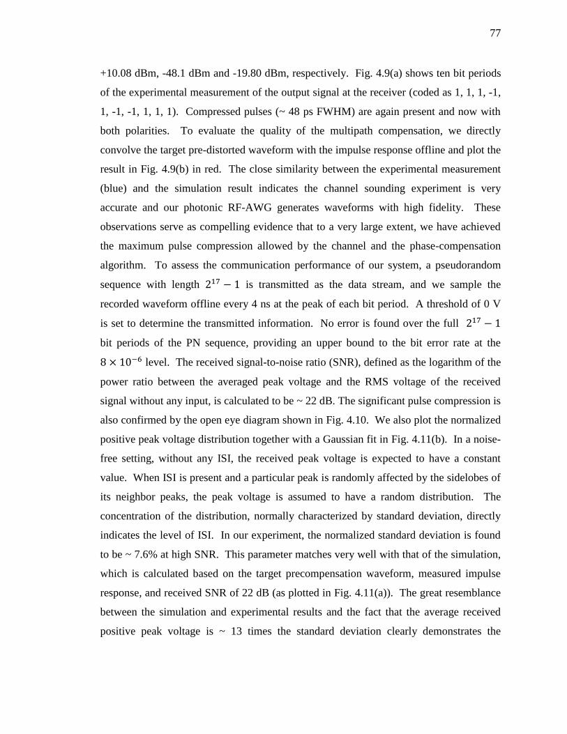
77
+10.08 dBm, -48.1 dBm and -19.80 dBm, respectively. Fig. 4.9(a) shows ten bit periods
of the experimental measurement of the output signal at the receiver (coded as 1, 1, 1, -1,
1, -1, -1, 1, 1, 1). Compressed pulses (~ 48 ps FWHM) are again present and now with
both polarities. To evaluate the quality of the multipath compensation, we directly
convolve the target pre-distorted waveform with the impulse response offline and plot the
result in Fig. 4.9(b) in red. The close similarity between the experimental measurement
(blue) and the simulation result indicates the channel sounding experiment is very
accurate and our photonic RF-AWG generates waveforms with high fidelity. These
observations serve as compelling evidence that to a very large extent, we have achieved
the maximum pulse compression allowed by the channel and the phase-compensation
algorithm. To assess the communication performance of our system, a pseudorandom
sequence with length 217 − 1 is transmitted as the data stream, and we sample the
recorded waveform offline every 4 ns at the peak of each bit period. A threshold of 0 V
is set to determine the transmitted information. No error is found over the full 217 − 1
bit periods of the PN sequence, providing an upper bound to the bit error rate at the
8 × 10⁻⁶ level. The received signal-to-noise ratio (SNR), defined as the logarithm of the
power ratio between the averaged peak voltage and the RMS voltage of the received
signal without any input, is calculated to be ~ 22 dB. The significant pulse compression is
also confirmed by the open eye diagram shown in Fig. 4.10. We also plot the normalized
positive peak voltage distribution together with a Gaussian fit in Fig. 4.11(b). In a noise-
free setting, without any ISI, the received peak voltage is expected to have a constant
value. When ISI is present and a particular peak is randomly affected by the sidelobes of
its neighbor peaks, the peak voltage is assumed to have a random distribution. The
concentration of the distribution, normally characterized by standard deviation, directly
indicates the level of ISI. In our experiment, the normalized standard deviation is found
to be ~ 7.6% at high SNR. This parameter matches very well with that of the simulation,
which is calculated based on the target precompensation waveform, measured impulse
response, and received SNR of 22 dB (as plotted in Fig. 4.11(a)). The great resemblance
between the simulation and experimental results and the fact that the average received
positive peak voltage is ~ 13 times the standard deviation clearly demonstrates the
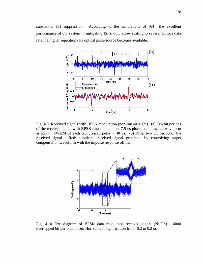
78
substantial ISI suppression. According to the simulations of [64], the excellent
performance of our system in mitigating ISI should allow scaling to several Gbits/s data
rate if a higher repetition rate optical pulse source becomes available.
Fig. 4.9 Received signals with BPSK modulation (non-line-of-sight). (a) Ten bit periods
of the received signal with BPSK data modulation, 7.5 ns phase-compensated waveform
as input. FWHM of each compressed pulse ~ 48 ps. (b) Blue: two bit period of the
received signal. Red: simulated received signal generated by convolving target
compensation waveform with the impulse response offline.
Fig. 4.10 Eye diagram of BPSK data modulated received signal (NLOS). 4000
overlapped bit periods. Inset: Horizontal magnification from -0.2 to 0.2 ns.
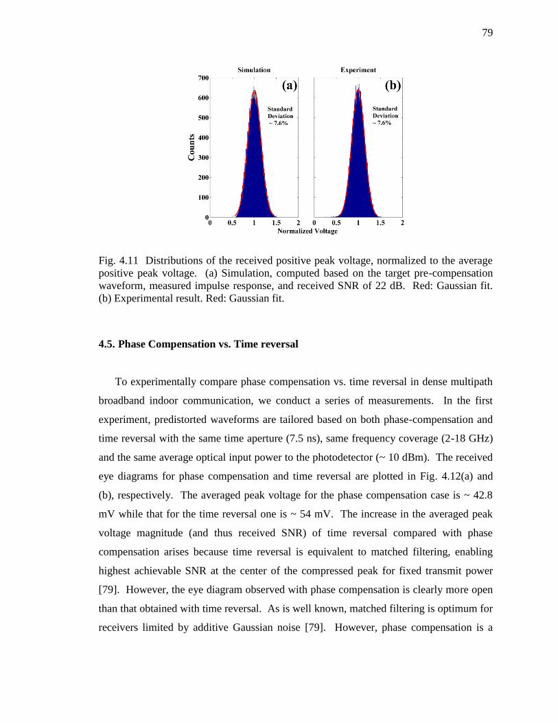
79
Fig. 4.11 Distributions of the received positive peak voltage, normalized to the average
positive peak voltage. (a) Simulation, computed based on the target pre-compensation
waveform, measured impulse response, and received SNR of 22 dB. Red: Gaussian fit.
(b) Experimental result. Red: Gaussian fit.
4.5. Phase Compensation vs. Time reversal
To experimentally compare phase compensation vs. time reversal in dense multipath
broadband indoor communication, we conduct a series of measurements. In the first
experiment, predistorted waveforms are tailored based on both phase-compensation and
time reversal with the same time aperture (7.5 ns), same frequency coverage (2-18 GHz)
and the same average optical input power to the photodetector (~ 10 dBm). The received
eye diagrams for phase compensation and time reversal are plotted in Fig. 4.12(a) and
(b), respectively. The averaged peak voltage for the phase compensation case is ~ 42.8
mV while that for the time reversal one is ~ 54 mV. The increase in the averaged peak
voltage magnitude (and thus received SNR) of time reversal compared with phase
compensation arises because time reversal is equivalent to matched filtering, enabling
highest achievable SNR at the center of the compressed peak for fixed transmit power
[79]. However, the eye diagram observed with phase compensation is clearly more open
than that obtained with time reversal. As is well known, matched filtering is optimum for
receivers limited by additive Gaussian noise [79]. However, phase compensation is a
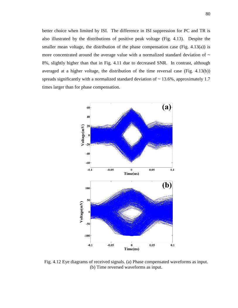
80
better choice when limited by ISI. The difference in ISI suppression for PC and TR is
also illustrated by the distributions of positive peak voltage (Fig. 4.13). Despite the
smaller mean voltage, the distribution of the phase compensation case (Fig. 4.13(a)) is
more concentrated around the average value with a normalized standard deviation of ~
8%, slightly higher than that in Fig. 4.11 due to decreased SNR. In contrast, although
averaged at a higher voltage, the distribution of the time reversal case (Fig. 4.13(b))
spreads significantly with a normalized standard deviation of ~ 13.6%, approximately 1.7
times larger than for phase compensation.
Fig. 4.12 Eye diagrams of received signals. (a) Phase compensated waveforms as input.
(b) Time reversed waveforms as input.
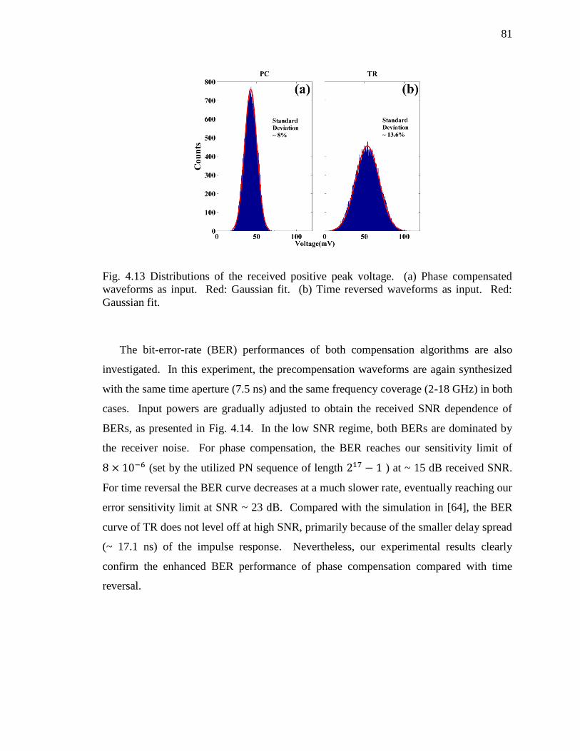
81
Fig. 4.13 Distributions of the received positive peak voltage. (a) Phase compensated
waveforms as input. Red: Gaussian fit. (b) Time reversed waveforms as input. Red:
Gaussian fit.
The bit-error-rate (BER) performances of both compensation algorithms are also
investigated. In this experiment, the precompensation waveforms are again synthesized
with the same time aperture (7.5 ns) and the same frequency coverage (2-18 GHz) in both
cases. Input powers are gradually adjusted to obtain the received SNR dependence of
BERs, as presented in Fig. 4.14. In the low SNR regime, both BERs are dominated by
the receiver noise. For phase compensation, the BER reaches our sensitivity limit of
8 × 10⁻⁶ (set by the utilized PN sequence of length 217 − 1 ) at ~ 15 dB received SNR.
For time reversal the BER curve decreases at a much slower rate, eventually reaching our
error sensitivity limit at SNR ~ 23 dB. Compared with the simulation in [64], the BER
curve of TR does not level off at high SNR, primarily because of the smaller delay spread
(~ 17.1 ns) of the impulse response. Nevertheless, our experimental results clearly
confirm the enhanced BER performance of phase compensation compared with time
reversal.
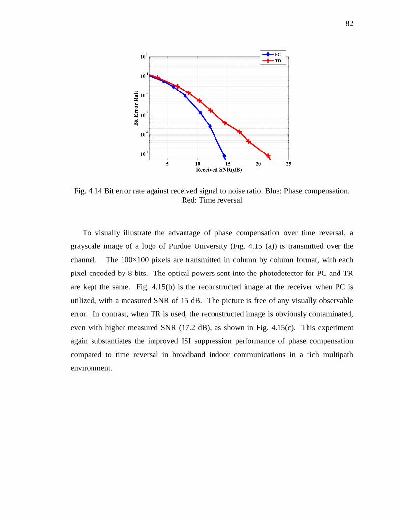
82
Fig. 4.14 Bit error rate against received signal to noise ratio. Blue: Phase compensation.
Red: Time reversal
To visually illustrate the advantage of phase compensation over time reversal, a
grayscale image of a logo of Purdue University (Fig. 4.15 (a)) is transmitted over the
channel. The 100×100 pixels are transmitted in column by column format, with each
pixel encoded by 8 bits. The optical powers sent into the photodetector for PC and TR
are kept the same. Fig. 4.15(b) is the reconstructed image at the receiver when PC is
utilized, with a measured SNR of 15 dB. The picture is free of any visually observable
error. In contrast, when TR is used, the reconstructed image is obviously contaminated,
even with higher measured SNR (17.2 dB), as shown in Fig. 4.15(c). This experiment
again substantiates the improved ISI suppression performance of phase compensation
compared to time reversal in broadband indoor communications in a rich multipath
environment.
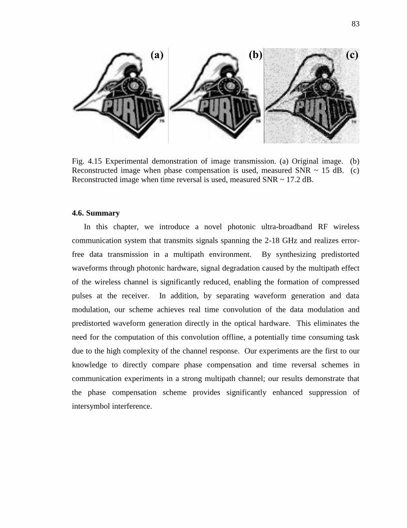
83
Fig. 4.15 Experimental demonstration of image transmission. (a) Original image. (b)
Reconstructed image when phase compensation is used, measured SNR ~ 15 dB. (c)
Reconstructed image when time reversal is used, measured SNR ~ 17.2 dB.
4.6. Summary
In this chapter, we introduce a novel photonic ultra-broadband RF wireless
communication system that transmits signals spanning the 2-18 GHz and realizes error-
free data transmission in a multipath environment. By synthesizing predistorted
waveforms through photonic hardware, signal degradation caused by the multipath effect
of the wireless channel is significantly reduced, enabling the formation of compressed
pulses at the receiver. In addition, by separating waveform generation and data
modulation, our scheme achieves real time convolution of the data modulation and
predistorted waveform generation directly in the optical hardware. This eliminates the
need for the computation of this convolution offline, a potentially time consuming task
due to the high complexity of the channel response. Our experiments are the first to our
knowledge to directly compare phase compensation and time reversal schemes in
communication experiments in a strong multipath channel; our results demonstrate that
the phase compensation scheme provides significantly enhanced suppression of
intersymbol interference.
84
5. REVIEW AND FUTURE RESEARCH DIRECTIONS
5.1. Review
In this work, we experimentally demonstrate advanced photonic techniques based on
optical pulse shaping and frequency-to-time mapping for various broadband radio
frequency applications. In Chapter 1, we introduce the unique advantages of broadband
radio frequency applications as well as the current obstacles that prevent the full
utilization of the potentials provided by the enormous bandwidth.
Chapter 2 focuses on the generation of arbitrary radio frequency waveforms using
ultrafast photonic techniques. Photonic RF-AWG based on optical pulse shaping and
FTM have generated impressive broadband waveforms, but with limited time aperture
and non-repeating period. This restriction constrains the synthesized waveforms in
applications such as unambiguous ranging and spread spectrum channel sounding with
severe multipath distortions. Two novel modulation techniques, namely amplitude
mismatched pseudorandom sequence modulation and phase shifted pseudorandom
sequence modulation, are proposed and mathematically studied to break the
aforementioned restriction and arbitrarily expand the time aperture of the generated
waveform. Experimental apparatuses based on differential detection and dual shapers are
assembled to employ these modulation schemes and generate arbitrary RF waveforms.
Arbitrary radio frequency waveforms, with wide frequency coverage (from DC up to ~
40 GHz), long time aperture and non-repeating period (up to ~ 4 microseconds) and high
average power (100% duty cycle) have been experimentally demonstrated. In addition,
the synthesized waveforms exhibit excellent long term stability and repeatability.
Furthermore, capitalizing on the scalability of the proposed photonic RF-AWG and the
ultra-high speed of a specially engineered photodetector, we extend the RF-AWG to the
microwave W-band. For the first time to our knowledge, arbitrary W-band waveforms
85
covering the full bandwidth and with microsecond level time aperture are experimentally
generated.
In Chapter 3, waveforms introduced in Chapter 2 are utilized in ranging experiments
to highlight the advantages of our proposed RF-AWG techniques. In 2 – 12 GHz
frequency band, ranging experiments are conducted to confirm the superiority of our
generated waveforms in delivering high average power and long unambiguous detection
range. In the microwave W-band, record 3.9 mm ranging resolution and up to ~ 9 m
unambiguous detection range are experimentally demonstrated using a photonic-assisted
ranging system.
Chapter 4 starts with addressing the need for multipath compensation in broadband
wireless communication. Based on the photonic RF-AWG system described in previous
chapter, a broadband communication system spanning the 2-18 GHz is proposed. This
system is capable of performing spread spectrum channel sounding, pre-compensation
based waveform generation and data modulation in optical hardware. Utilizing such
system, error-free data transmissions in both OOK and BPSK formats are accomplished
at 250 Mbits/sec. This result, to my knowledge, was the first experimental demonstration
of photonic-assisted broadband wireless communication in a highly complex and dense
multipath indoor environment. In addition, our experiments are the first to our
knowledge to directly compare phase compensation and time reversal schemes in
communication experiments in a strong multipath channel; our results demonstrate that
the phase compensation scheme provides significantly enhanced suppression of
intersymbol interference. We believe our work is a significant step towards the next
generation ultra-broadband wireless communication.
5.2. Future Research Directions
One interesting research direction is to increase the data rate of the current wireless
communication system introduced in Chapter 4, especially the NLOS one which is of
greater interest. In [64], simulation results based on multiple NLOS channel impulse
responses with an average RMS delay of 19 ns suggested that a wireless communications
system can operate at a data rate of 1 Gbits/sec without exhibiting an error floor in the
86
BER curve. Considering the fact that our channel has a shorter RMS delay (~ 17 ns) and
thus less channel distortion, a data rate of 1 Gbits/sec should be readily achievable by
using a higher repetition optical source. A special engineering effort is required to
assemble such a broadband optical source. Subsequently, further investigation on the
wireless channel is needed to provide a comprehensive understanding of the
communication system. For instance, broadband communication is usually characterized
by limited spatial coherence. Data transmission will be completely disrupted with even a
few decimeters displacement of the receiver [44]. As a result, a time-varying channel or
a moving receiver poses extra requirements on the configurability of the system.
Another interesting aspect to investigate is the cell area. The distribution of the
wireless accessing points directly dictates the complexity of the wireless channel for each
receiver, which eventually determines the maximum achievable data rate. For instance, if
there is at least one accessing point in each room, the wireless channel between the
accessing point and the receiver will always stay in line-of-sight. The reduced
complexity of this type of channel compared with non-line-of-sight ones may enable
much higher data rate and fast processing speed for the central office.
Last but not the least, integration of the photonically enabled broadband wireless
communication system is another long term research direction. From the ROF point of
view, it is important that both the central office transmitter and receiving device be
created with reasonable physical size and efficient power consumption. Si-photonics has
demonstrated great potentials in the integration of optical functionalities and should be
considered as the most promising approach.

LIST OF REFERENCES
87
LIST OF REFERENCES
[1] T. W. Barrett, "History of ultrawideband (UWB) radar & communications: pioneers
and innovators," in Proc. Progress in Electromagnetics Symposium, 2000, pp. 1-42.
[2] A. B. Carlson and P. B. Crilly, Communication systems. New York (N.Y.): McGraw-
Hill, 2010.
[3] M. G. Di Benedetto, UWB communication systems: a comprehensive overview vol.
5: Hindawi Publishing Corporation, 2006.
[4] T. F. Tseng, J. M. Wun, W. Chen, S. W. Peng, J. W. Shi, and C. K. Sun, "High-
depth-resolution 3-dimensional radar-imaging system based on a few-cycle W-band
photonic millimeter-wave pulse generator," Optics Express, vol. 21, pp. 14109-
14119, Jun 17 2013.
[5] Y. Kado and T. Nagatsuma, "Exploring sub-THz waves for communications,
imaging, and gas sensing," Piers 2009 Beijing: Progess in Electromagnetics
Research Symposium, Proceedings I and Ii, pp. 42-47, 2009.
[6] J. Federici and L. Moeller, "Review of terahertz and subterahertz wireless
communications," Journal of Applied Physics, vol. 107, Jun 1 2010.
[7] J. W. Shi, C. B. Huang, and C. L. Pan, "Millimeter-wave photonic wireless links for
very high data rate communication," NPG Asia Materials, vol. 3, pp. 41-48, Apr
2011.
[8] N. W. Chen, J. W. Shi, H. J. Tsai, J. M. Wun, F. M. Kuo, J. Hesler, et al., "Design
and demonstration of ultra-fast W-band photonic transmitter-mixer and detectors for
25 Gbits/sec error-free wireless linking," Optics Express, vol. 20, pp. 21223-21234,
Sep 10 2012.
[9] X. Y. Li, Z. Dong, J. J. Yu, N. Chi, Y. F. Shao, and G. K. Chang, "Fiber-wireless
transmission system of 108 Gb/s data over 80 km fiber and 2 x 2 multiple-input
multiple-output wireless links at 100 GHz W-band frequency," Optics Letters, vol.
37, pp. 5106-5108, Dec 15 2012.
[10] S. Koenig, D. Lopez-Diaz, J. Antes, F. Boes, R. Henneberger, A. Leuther, et al.,
"Wireless sub-THz communication system with high data rate," Nature Photonics,
vol. 7, pp. 977-981, Dec 2013.
[11] T. Nagatsuma, S. Horiguchi, Y. Minamikata, Y. Yoshimizu, S. Hisatake, S. Kuwano,
et al., "Terahertz wireless communications based on photonics technologies," Optics
Express, vol. 21, pp. 23736-23747, Oct 7 2013.
[12] K. B. Cooper, R. J. Dengler, N. Llombart, T. Bryllert, G. Chattopadhyay, E.
Schlecht, et al., "Penetrating 3-D imaging at 4-and 25-m range using a
submillimeter-wave radar," IEEE Transactions on Microwave Theory and
Techniques, vol. 56, pp. 2771-2778, Dec 2008.
88
[13] K. B. Cooper, R. J. Dengler, N. Llombart, A. Talukder, A. V. Panangadan, C. S.
Peay, et al., "Fast, high-resolution terahertz radar imaging at 25 meters," Terahertz
Physics, Devices, and Systems IV: Advanced Applications in Industry and Defense,
vol. 7671, 2010.
[14] R. W. McMillan, "Terahertz imaging, millimeter-wave radar," Advances in Sensing
with Security Applications, vol. 2, pp. 243-268, 2006.
[15] M. Tonouchi, "Cutting-edge terahertz technology," Nature Photonics, vol. 1, pp. 97-
105, Feb 2007.
[16] J. A. Zeitler and L. F. Gladden, "In-vitro tomography and non-destructive imaging at
depth of pharmaceutical solid dosage forms," European Journal of Pharmaceutics
and Biopharmaceutics, vol. 71, pp. 2-22, Jan 2009.
[17] D. M. Sheen, J. L. Fernandes, J. R. Tedeschi, D. L. McMakin, A. M. Jones, W. M.
Lechelt, et al., "Wide-bandwidth, wide-beamwidth, high-resolution, millimeter-wave
imaging for concealed weapon detection," Passive and Active Millimeter-Wave
Imaging XVI, vol. 8715, 2013.
[18] H. J. Hansen, "Standoff detection using millimeter and submillimeter wave
spectroscopy," Proceedings of the IEEE, vol. 95, pp. 1691-1704, Aug 2007.
[19] L. Chao, M. N. Afsar, and K. A. Korolev, "Millimeter wave dielectric spectroscopy
and breast cancer imaging," 2012 7th European Microwave Integrated Circuits
Conference (Eumic), pp. 572-575, 2012.
[20] J. L. Neill, B. J. Harris, A. L. Steber, K. O. Douglass, D. F. Plusquellic, and B. H.
Pate, "Segmented chirped-pulse Fourier transform submillimeter spectroscopy for
broadband gas analysis," Optics Express, vol. 21, pp. 19743-19749, Aug 26 2013.
[21] A. P. Colombo, Y. Zhou, K. Prozument, S. L. Coy, and R. W. Field, "Chirped-pulse
millimeter-wave spectroscopy: Spectrum, dynamics, and manipulation of Rydberg-
Rydberg transitions," Journal of Chemical Physics, vol. 138, Jan 7 2013.
[22] Tektronix. Radio-Frequency Arbitrary Waveform Generator - AWG70000A.
Available: HTTP://WWW.TEK.COM/DATASHEET/AWG70000A/AWG70000A-SERIES-
DATASHEET [23] J. D. McKinney and A. M. Weiner, "Photonic synthesis of ultrabroadband arbitrary
electromagnetic waveforms," in Microwave Photonics, C. H. Lee, Ed., ed: CRC
Press, 2013.
[24] J. P. Yao, "Photonics for ultrawideband communications," IEEE Microwave
Magazine, vol. 10, pp. 82-95, Jun 2009.
[25] J. D. McKinney, D. E. Leaird, and A. M. Weiner, "Millimeter-wave arbitrary
waveform generation with a direct space-to-time pulse shaper," Optics Letters, vol.
27, pp. 1345-1347, Aug 1 2002.
[26] J. Chou, Y. Han, and B. Jalali, "Adaptive RF-photonic arbitrary waveform
generator," IEICE Transactions on Electronics, vol. E86c, pp. 1226-1229, Jul 2003.
[27] I. S. Lin, J. D. McKinney, and A. M. Weiner, "Photonic synthesis of broadband
microwave arbitrary waveforms applicable to ultra-wideband communication," IEEE
Microwave and Wireless Components Letters, vol. 15, pp. 226-228, Apr 2005.
[28] C. B. Huang, D. E. Leaird, and A. M. Weiner, "Time-multiplexed photonically
enabled radio-frequency arbitrary waveform generation with 100 ps transitions,"
Optics Letters, vol. 32, pp. 3242-3244, Nov 15 2007.

89
[29] C. M. Long, D. E. Leaird, and A. M. Weiner, "Photonically enabled agile rf
waveform generation by optical comb shifting," Optics Letters, vol. 35, pp. 3892-
3894, Dec 1 2010.
[30] C. Wang and J. P. Yao, "Large time-bandwidth product microwave arbitrary
waveform generation using a spatially discrete chirped fiber bragg grating," Journal
of Lightwave Technology, vol. 28, pp. 1652-1660, Jun 1 2010.
[31] J. M. Wun, C. C. Wei, J. H. Chen, C. S. Goh, S. Y. Set, and J. W. Shi, "Photonic
chirped radio-frequency generator with ultra-fast sweeping rate and ultra-wide
sweeping range," Optics Express, vol. 21, pp. 11475-11481, May 6 2013.
[32] H. Al-Raweshidy and S. Komaki, Radio over fiber technologies for mobile
communications networks: Artech House, 2002.
[33] V. Torres-Company, A. J. Metcalf, D. E. Leaird, and A. M. Weiner, "Multichannel
radio-frequency arbitrary waveform generation based on multiwavelength comb
wwitching and 2-D line-by-line pulse shaping," IEEE Photonics Technology Letters,
vol. 24, pp. 891-893, Jun 1 2012.
[34] V. Torres-Company and A. M. Weiner, "Optical frequency comb technology for
ultra-broadband radio-frequency photonics," Laser & Photonics Reviews, vol.8, pp
368-393, May 2014.
[35] A. M. Weiner, "Ultrafast optical pulse shaping: a tutorial review," Optics
Communications, vol. 284, pp. 3669-3692, Jul 15 2011.
[36] A. Dezfooliyan and A. M. Weiner, "Photonic synthesis of high fidelity microwave
arbitrary waveforms using near field frequency to time mapping," Optics Express,
vol. 21, pp. 22974-22987, Sep 23 2013.
[37] V. Torres-Company, D. E. Leaird, and A. M. Weiner, "Dispersion requirements in
coherent frequency-to-time mapping," Optics Express, vol. 19, pp. 24718-24729,
Nov 21 2011.
[38] J. R. Klauder, A. C. Price, S. Darlington, and W. J. Albersheim, "The theory and
design of chirp radars," Bell System Technical Journal, vol. 39, pp. 745-808, 1960.
[39] Y. Li, A. Dezfooliyan, and A. M. Weiner, "Photonic synthesis of spread spectrum
radio frequency waveforms with arbitrarily long time apertures," Lightwave
Technology, Journal of, vol. 32, pp. 3580-3587, 2014.
[40] F. J. Macwilliams and N. J. A. Sloane, "Pseudo-random sequences and arrays,"
Proceedings of the IEEE, vol. 64, pp. 1715-1730, 1976.
[41] S. R. J. Axelsson, "Noise radar using random phase and frequency modulation,"
IEEE Transactions on Geoscience and Remote Sensing, vol. 42, pp. 2370-2384, Nov
2004.
[42] A. W. Rihaczek, Principles of high-resolution radar. New York,: McGraw-Hill,
1969.
[43] R. Zetik, J. Sachs, and R. S. Thoma, "UWB short-range radar sensing," IEEE
Instrumentation & Measurement Magazine, vol. 10, pp. 39-45, Apr 2007.
[44] A. Dezfooliyan and A. M. Weiner, "Microwave photonics for space-time
compression of ultrabroadband signals through multipath wireless channels," Optics
Letters, vol. 38, pp. 4946-4949, Dec 1 2013.
[45] R. N. Bracewell, The Fourier Transform and Its Applications: McGraw Hill, 2000.
90
[46] J. D. McKinney, "Background-free arbitrary waveform generation via polarization
pulse shaping," IEEE Photonics Technology Letters, vol. 22, pp. 1193-1195, Aug 15
2010.
[47] Y. Li, A. Rashidinejad, J.-M. Wun, D. E. Leaird, J.-W. Shi, and A. M. Weiner,
"Photonic generation of W-band arbitrary waveforms with high time-bandwidth
products enabling 3.9mm range resolution," Optica, vol. 1, pp. 446-454, 2014/12/20
2014.
[48] L. A. Samoska, "An overview of solid-state integrated circuit amplifiers in the
submillimeter-wave and THz regime," IEEE Transactions on Terahertz Science and
Technology, vol. 1, pp. 9-24, Sep 2011.
[49] A. Kanno and T. Kawanishi, "Broadband frequency-modulated continuous-wave
signal generation by optical modulation technique," Lightwave Technology, Journal
of, vol. PP, pp. 1-1, 2014.
[50] A. J. Seeds and K. J. Williams, "Microwave photonics," Journal of Lightwave
Technology, vol. 24, pp. 4628-4641, Dec 2006.
[51] J. Capmany and D. Novak, "Microwave photonics combines two worlds," Nature
Photonics, vol. 1, pp. 319-330, Jun 2007.
[52] F. Quinlan, T. M. Fortier, H. Jiang, A. Hati, C. Nelson, Y. Fu, et al., "Exploiting shot
noise correlations in the photodetection of ultrashort optical pulse trains," Nature
Photonics, vol. 7, pp. 290-293, Apr 2013.
[53] T. M. Fortier, M. S. Kirchner, F. Quinlan, J. Taylor, J. C. Bergquist, T. Rosenband,
et al., "Generation of ultrastable microwaves via optical frequency division," Nature
Photonics, vol. 5, pp. 425-429, Jul 2011.
[54] J. W. Shi, F. M. Kuo, and J. E. Bowers, "Design and analysis of ultra-high-speed
near-ballistic uni-traveling-carrier photodiodes under a 50-Omega load for high-
power performance," IEEE Photonics Technology Letters, vol. 24, pp. 533-535, Apr
1 2012.
[55] N.-W. Chen, H.-J. Tsai, F.-M. Kuo, and J.-W. Shi, "High-speed-band integrated
photonic transmitter for radio-over-fiber applications," Microwave Theory and
Techniques, IEEE Transactions on, vol. 59, pp. 978-986, 2011.
[56] A. Rashidinejad, Y. Li, J.-M. Wun, D. E. Leaird, J.-W. Shi, and A. M. Weiner,
"Photonic generation and wireless transmission of W-band arbitrary waveforms with
high time-bandwidth products," in CLEO: 2014, San Jose, California, 2014, p.
SM1G.1.
[57] N. Levanon, "Radar principles," New York, Wiley-Interscience, 1988, 320 p., vol. 1,
1988.
[58] J. W. Shi, F. M. Kuo, N. W. Chen, S. Y. Set, C. B. Huang, and J. E. Bowers,
"Photonic generation and wireless transmission of linearly/nonlinearly continuously
tunable chirped millimeter-wave waveforms with high time-bandwidth product at
W-band," IEEE Photonics Journal, vol. 4, pp. 215-223, Feb 2012.
[59] H. B. Gao, C. Lei, M. H. Chen, F. J. Xing, H. W. Chen, and S. Z. Xie, "A simple
photonic generation of linearly chirped microwave pulse with large time-bandwidth
product and high compression ratio," Optics Express, vol. 21, pp. 23107-23115, Oct
7 2013.
91
[60] S. T. Cundiff and A. M. Weiner, "Optical arbitrary waveform generation," Nature
Photonics, vol. 4, pp. 760-766, Nov 2010.
[61] R. J. Fontana, "Recent system applications of short-pulse ultra-wideband (UWB)
technology," Microwave Theory and Techniques, IEEE Transactions on, vol. 52, pp.
2087-2104, 2004.
[62] J. D. McKinney, D. Peroulis, and A. M. Weiner, "Dispersion limitations of ultra-
wideband wireless links and their compensation via photonically enabled arbitrary
waveform generation," IEEE Transactions on Microwave Theory and Techniques,
vol. 56, pp. 710-719, Mar 2008.
[63] J. D. McKinney and A. M. Weiner, "Compensation of the effects of antenna
dispersion on UWB waveforms via optical pulse-shaping techniques," IEEE
Transactions on Microwave Theory and Techniques, vol. 54, pp. 1681-1686, Apr
2006.
[64] A. Dezfooliyan and A. M. Weiner, "Phase compensation communication technique
against time reversal for ultra-wideband channels," IET Communications, vol. 7, pp.
1287-1295, Aug 13 2013.
[65] N. Levanon and E. Mozeson, Radar signals: John Wiley & Sons, 2004.
[66] A. Rashidinejad and A. M. Weiner, "Photonic radio-frequency arbitrary waveform
generation with maximal time-bandwidth product capability," Journal of Lightwave
Technology, vol. 32, pp. 3383-3393, Oct 15 2014.
[67] A. Y. Nashashibi, K. Sarabandi, P. Frantzis, R. D. De Roo, and F. T. Ulaby, "An
ultrafast wide-band millimeter-wave (MMW) polarimetric radar for remote sensing
applications," IEEE Transactions on Geoscience and Remote Sensing, vol. 40, pp.
1777-1786, Aug 2002.
[68] H. Essen, M. Hägelen, A. Wahlen, K. Schulz, K. Jäger, and M. Hebel, "ISAR
imaging of helicopters using millimeter wave radars," International Journal of
Microwave and Wireless Technologies, vol. 1, pp. 171-178, 2009.
[69] E. Rubiola, Phase noise and frequency stability in oscillators. Cambridge, UK ; New
York: Cambridge University Press, 2009.
[70] X. B. Yu, T. B. Gibbon, R. Rodes, T. T. Pham, and I. T. Monroy, "System wide
implementation of photonically generated impulse radio ultra-wideband for gigabit
fiber-wireless access," Journal of Lightwave Technology, vol. 31, pp. 264-275, Jan
15 2013.
[71] R. R. Lopez, A. Caballero, X. B. Yu, T. B. Gibbon, J. B. Jensen, and I. T. Monroy,
"A comparison of electrical and photonic pulse generation for IR-UWB on fiber
links," IEEE Photonics Technology Letters, vol. 22, pp. 263-265, Mar 1 2010.
[72] S. L. Pan and J. P. Yao, "UWB-over-fiber communications: modulation and
transmission," Journal of Lightwave Technology, vol. 28, pp. 2445-2455, Aug 15
2010.
[73] H. Shams, A. Kaszubowska-Anandarajah, P. Perry, and L. P. Barry, "Optical
generation, fiber distribution and air transmission for ultra wide band over fiber
system," Ofc: 2009 Conference on Optical Fiber Communication, Vols 1-5, pp.
2814-2816, 2009.
92
[74] I. H. Naqvi, G. El Zein, G. Lerosey, J. de Rosny, P. Besnier, A. Tourin, et al.,
"Experimental validation of time reversal ultra wide-band communication system for
high data rates," IET Microwaves Antennas & Propagation, vol. 4, pp. 643-650,
May 2010.
[75] J. R. Foerster, "The effects of multipath interference on the performance of UWB
systems in an indoor wireless channel," IEEE VTC 53rd Vehicular Technology
Conference, Spring 2001, Vols 1-4, Proceedings, pp. 1176-1180, 2001.
[76] A. Dezfooliyan and A. M. Weiner, "Evaluation of time domain propagation
measurements of UWB systems using spread spectrum channel sounding," Antennas
and Propagation, IEEE Transactions on, vol. 60, pp. 4855-4865, 2012.
[77] A. F. Molisch, "Ultrawideband propagation channels-theory, measurement, and
modeling," Vehicular Technology, IEEE Transactions on, vol. 54, pp. 1528-1545,
2005.
[78] Y. Li and A. M. Weiner, "Photonic-assisted broadband wireless communication with
on-line channel compression," in Optical Fiber Communication Conference, Los
Angeles, California, 2015, p. W3F.3.
[79] M. B. Pursley, Introduction to digital communications. Upper Saddle River, NJ:
Pearson/Prentice Hall, 2005.

VITA
93
VITA
Yihan Li was born in Xuzhou, China in 1988. He received the B.S. degree in
Optical Information Science and Technology from the University of Science and
Technology of China (USTC), Hefei, China, in 2010.
From 2008 to 2010 he was a Research Assistant with the Key Laboratory of
Optoelectronic Science and Technology, USTC, Hefei, China. He joined Institute of
Physics, Chinese Academy of Science, Beijing, China, as a Research Assistant briefly in
2010. Since 2010, he has been a Ph.D. student and a Research Assistant with the
Ultrafast Optics and Optical Fiber Communications Laboratory, Purdue University, West
Lafayette. His research interests include ultrafast optics, optical pulse shaping,
microwave photonics and wideband RF wireless communications.