PHOTOMETRIC STEREO SHAPE-AND-ALBEDO … · PHOTOMETRIC STEREO SHAPE-AND-ALBEDO-FROM-SHADING FOR PIXEL-LEVEL RESOLUTION LUNAR SURFACE RECONSTRUCTION Wai Chung Liu, Bo Wu* Dept. of

PHOTOMETRIC STEREO SHAPE-AND-ALBEDO-FROM-SHADING FOR PIXEL-

LEVEL RESOLUTION LUNAR SURFACE RECONSTRUCTION

Wai Chung Liu, Bo Wu*

Dept. of Land Surveying and Geo-Informatics, Faculty of Construction and Environment, The Hong Kong Polytechnic University,

Hung Hom, Hong Kong – [email protected]; [email protected]

Commission III, ICWG III/II

KEY WORDS: Moon, DEM, Shape and Albedo from Shading, Photometric Stereo, LROC NAC

ABSTRACT:

Shape and Albedo from Shading (SAfS) techniques recover pixel-wise surface details based on the relationship between terrain

slopes, illumination and imaging geometry, and the energy response (i.e., image intensity) captured by the sensing system. Multiple

images with different illumination geometries (i.e., photometric stereo) can provide better SAfS surface reconstruction due to the

increase in observations. Photometric stereo SAfS is suitable for detailed surface reconstruction of the Moon and other extra-

terrestrial bodies due to the availability of photometric stereo and the less complex surface reflecting properties (i.e., albedo) of the

target bodies as compared to the Earth. Considering only one photometric stereo pair (i.e., two images), pixel-variant albedo is still a

major obstacle to satisfactory reconstruction and it needs to be regulated by the SAfS algorithm. The illumination directional

difference between the two images also becomes an important factor affecting the reconstruction quality. This paper presents a

photometric stereo SAfS algorithm for pixel-level resolution lunar surface reconstruction. The algorithm includes a hierarchical

optimization architecture for handling pixel-variant albedo and improving performance. With the use of Lunar Reconnaissance

Orbiter Camera - Narrow Angle Camera (LROC NAC) photometric stereo images, the reconstructed topography (i.e., the DEM) is

compared with the DEM produced independently by photogrammetric methods. This paper also addresses the effect of illumination

directional difference in between one photometric stereo pair on the reconstruction quality of the proposed algorithm by both

mathematical and experimental analysis. In this case, LROC NAC images under multiple illumination directions are utilized by the

proposed algorithm for experimental comparison. The mathematical derivation suggests an illumination azimuthal difference of 90

degrees between two images is recommended to achieve minimal error in SAfS reconstruction while results using real data presents

similar pattern. Although the algorithm is designed for lunar surface reconstruction, it is likely to be applicable on other extra-

terrestrial bodies such as Mars. The results and findings from this research is of significance for the practical use of photometric

stereo and SAfS in the domain of planetary remote sensing and mapping.

1. INTRODUCTION

Shape and Albedo from Shading (SAfS) is characterized by its

ability to reconstruct 3D shapes with subtle details on an image.

It is able to produce DEMs and other 3D shapes with resolution

comparable to the image(s). SAfS utilizes the relationship

between 3D geometry and energy reflection for reconstruction,

and therefore it also works on single image shape recovery. The

geometric information retrieval from SAfS can be less stable

compared to other modelling techniques such as

photogrammetry and laser altimetry, this is because SAfS deals

with the relative difference between adjacent pixels and extra

uncertainties are introduced by the reflecting behaviour of

surface material (i.e., reflectance models and albedo). Yet, it is

able to produce terrain models where other modelling

techniques are not available, and with details better than those

techniques (Wu et al., 2017).

SAfS techniques depend largely on the understanding of

reflectance models which describe the relationship between

surface orientation and energy response. This research has been

long studied and various practical models were developed

(McEwen, 1991; Hapke, 2002). Horn (1977; 1990) studied and

formulated the algorithm for shape recovery from shading

information; the use of SfS techniques in lunar mapping was

also suggested (Horn, 1990) due to the less complex surface

albedo on moon and perhaps other extra-terrestrial bodies.

Grumpe et al. (2014) and Wu et al. (2017) combined and

regulated SfS or SAfS by low-resolution lunar DEMs obtained

from photogrammetry and laser altimetry. This strategy allows

generation of pixel-level resolution lunar DEMs with their

overall geometry comparable to the low-resolution DEMs.

Photometric stereo refers to imaging the same object under

different illumination conditions (Woodham, 1980), shading

from various illumination direction can provide extra

information about the underlying shape and thus improving the

quality of 3D reconstruction. Woodham (1980) developed the

basic theory of photometric stereo as a way to obtain surface

orientation and verified with synthetic examples. Lohse and

Heipke (2004) developed the Multi-Image Shape from Shading

(MI-SfS) algorithm for lunar mapping. The core concept of MI-

SfS is similar to photometric stereo and they were able to

produce high resolution lunar DEMs where image matching

fails due to less distinctive texture.

In photometric stereo the azimuthal differences between

illumination directions may affect the quality of reconstruction,

this is more apparent when only one photometric stereo pair

(i.e., two images) is available. This paper firstly describes an

iterative hierarchical SAfS algorithm using photometric stereo,

followed by the mathematical derivation of the effect of

illumination azimuthal differences on SAfS performance. The

derivation is then verified by real data using LROC NAC

images and the described SAfS algorithm. Each of the SAfS

results only utilizes one pair of photometric stereo (i.e., double

image SAfS). The analysis and findings are concluded

afterwards.

The International Archives of the Photogrammetry, Remote Sensing and Spatial Information Sciences, Volume XLII-3/W1, 2017 2017 International Symposium on Planetary Remote Sensing and Mapping, 13–16 August 2017, Hong Kong

This contribution has been peer-reviewed. https://doi.org/10.5194/isprs-archives-XLII-3-W1-91-2017 | © Authors 2017. CC BY 4.0 License. 91

mailto:[email protected]

mailto:[email protected]

2. PHOTOMETRIC STEREO SAFS

2.1 Overview of approach

Photometric stereo SAfS majorly contains two steps: (1)

Gradient estimation from reflectance; and (2) Shape

reconstruction from gradients. The first step ‘Gradient

estimation from reflectance’ estimates the surface normal of

each pixel base on the image intensity, geometric reflectance

function and albedo. The output of this step is a vector field and

each vector on the field represents a surface normal. This

surface normal field is able to reproduce the captured image

through the geometric reflectance function and the albedo. The

second step ‘Shape reconstruction from gradients’ generates the

DEM according to the computed surface normal by evaluating

the relationship between adjacent height nodes. After this step,

the DEM should inherit as much information in the surface

normal field as possible and will be able to preserve subtle

details on the images.

The algorithm uses a hierarchical optimization strategy by

down-sampling the images and an initial DEM (i.e., can be

initialized by a flat plane, etc.) before SAfS and increases its

resolution by a factor of 2 iteratively until it reaches the desired

resolution. The current architecture is also named Cascade

Multi-grid (Capanna et al., 2013) which will not revisit and

optimize lower resolution components again; however general

control throughout all hierarchies is present to regulate

optimization. Optimization per hierarchy is iterative and will

terminate when stopping criteria is satisfied. The reconstruction

adopts the Modified Jacobi relaxation scheme (Horn, 1990) to

balance between convergence and data inter-dependencies.

2.2 Reflectance-based shape reconstruction

Shape reconstruction from shading information depends on the

relationship between the surface normal of the object (i.e.,

slopes and aspects) and the intensity captured by sensors under

certain illumination and imaging geometry. The illumination

and imaging conditions are usually known as assumed in this

article. At any pixel, the recorded intensity I can be expressed

as:

𝐼 = 𝐴𝐺(𝑝, 𝑞) (1)

where 𝐼 = image intensity

𝐴= albedo

𝐺(𝑝, 𝑞) = geometric reflectance function

Albedo A represents the ability of the surface material to scatter

or reflect incoming light. The value of albedo lies between zero

to unity while it is very unlikely that (A = 0). The value of

albedo can be obtained empirically or be estimated using certain

initial estimates of the underlying shape (e.g., assuming to be a

flat plane initially). 𝐺(𝑝, 𝑞) denotes the geometric reflectance

function which relates surface normal (p,q) of a point and its

reflectance. Well-known reflectance models include the

Lambertian model, the Lunar-Lambertian model

(McEwen,1991) and Hapke model (Hapke, 2002). The surface

normal (p,q) of a point is described by the partial derivatives

(i.e., tangent) of the surface (𝑍 = 𝑆(𝑥, 𝑦)) along x- and y-

direction at that point:

𝑝 = 𝜕𝑆(𝑥,𝑦)

𝜕𝑥; 𝑞 =

𝜕𝑆(𝑥,𝑦)

𝜕𝑦 (2)

Given certain initial estimate of the surface normal [𝑝0

𝑞0] and

albedo A, the observation equation can be setup by linearizing

𝐺(𝑝, 𝑞) to solve for iterative update of the surface normal:

𝜕𝐺0

𝜕𝑝∆𝑝 +

𝜕𝐺0

𝜕𝑞∆𝑞 =

𝐼

𝐴− 𝐺0 (3)

where 𝐺0 = 𝐺(𝑝0, 𝑞0)

∆𝑝 = update for p

∆𝑞 = update for q

With multiple images (i.e., photometric stereo pairs), a set of

equation (3), one for each image, can be setup and the

optimization can be expressed as minimizing the error term:

∑ (𝐺0|𝑘 +𝜕𝐺0

𝜕𝑝|𝑘∆𝑝 +

𝜕𝐺0

𝜕𝑞|𝑘∆𝑞 −

𝐼𝑘

𝐴)2

𝑘1 (4)

where (𝑘 ≥ 2) = number of available image

A vector field representing the surface normal at each pixel is

produced after the aforementioned optimization. Shape recovery

from surface normal requires the surface normal field to be

integrable, which is formulated as:

𝜕𝑝

𝜕𝑦=

𝜕𝑞

𝜕𝑥 (5)

This implies that for all possible routes between any two points

on a surface, the integrated (i.e., summed) height differences of

each route must be identical. Some works enforce such

condition directly on the surface normal field (Frankot and

Chellappa, 1988; Horn, 1990). This research enforces

integrability by directly adjusting the elevation nodes of the

underlying DEM such that the DEM best represents the surface

normal vector field resulted from equation (4). The pixel-variant

albedo can be retrieved from the optimized SAfS DEM and the

images.

3. EFFECT OF ILLUMINATION DIRECTIONAL

DIFFERENCE TO PHOTOMETRIC STEREO SAFS

3.1 Derivation of Photometric Stereo SAfS solution

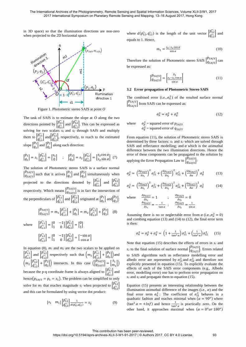
Considering any single point O on a surface, photometric stereo

SAfS estimates its surface normal by evaluating the slope of O

along each of the available illumination directions. Now

consider Figure 1 for the case of only one photometric stereo

pair is available (i.e., double image SAfS): centring at point O, a

unit vector [𝑝𝐿1̂

𝑞𝐿1̂] is pointing towards the illumination direction 1,

the horizontal axis p of the Cartesian coordinate frame is

aligned to [𝑝𝐿1̂

𝑞𝐿1̂] so that ([

𝑝𝐿1̂

𝑞𝐿1̂] = [

10]) . Another unit vector

[𝑝𝐿2̂

𝑞𝐿2̂] is pointing towards illumination direction 2 which is 𝛼

degrees counter-clockwise from illumination direction 1. The

relationship between the two unit vectors can be denoted as:

[𝑝𝐿2̂

𝑞𝐿2̂] = 𝑅(𝛼) [

𝑝𝐿1̂

𝑞𝐿1̂] = [

cos 𝛼 − sin 𝛼sin 𝛼 cos 𝛼

] [10] = [

cos𝛼sin 𝛼

] (6)

The term 𝛼 is the azimuthal difference between the two

illumination directions, 𝛼 is negative when the rotation is in

clock-wise direction. It is assumed that the zenith angles of both

illumination sources are non-zero (i.e., not parallel to the Z-axis


This contribution has been peer-reviewed. https://doi.org/10.5194/isprs-archives-XLII-3-W1-91-2017 | © Authors 2017. CC BY 4.0 License.

92

in 3D space) so that the illumination directions are non-zero

when projected to the 2D horizontal space.

Figure 1. Photometric stereo SAfS at point O

The task of SAfS is to estimate the slope at O along the two

directions pointed by [𝑝𝐿1̂

𝑞𝐿1̂] and [

𝑝𝐿2̂

𝑞𝐿2̂]. This can be expressed as

solving for two scalars s1 and s2 through SAfS and multiply

them to [𝑝𝐿1̂

𝑞𝐿1̂] and[

𝑝𝐿2̂

𝑞𝐿2̂], respectively, to reach to the estimated

slope [𝑝1

𝑞1] and [

𝑝2

𝑞2] along each direction:

[𝑝1

𝑞1] = 𝑠1 [

𝑝𝐿1̂

𝑞𝐿1̂] = [

𝑠1

0] ; [

𝑝2

𝑞2] = 𝑠2 [

𝑝𝐿2̂

𝑞𝐿2̂] = [

𝑠2cos 𝛼𝑠2 sin 𝛼] (7)

The solution of Photometric stereo SAfS is a surface normal

[𝑝𝑆𝐴𝑓𝑆

𝑞𝑆𝐴𝑓𝑆] such that it arrives [

𝑝1

𝑞1] and [

𝑝2

𝑞2] simultaneously when

projected to the directions denoted by [𝑝𝐿1̂

𝑞𝐿1̂] and [

𝑝𝐿2̂

𝑞𝐿2̂]

respectively. Which means [𝑝𝑆𝐴𝑓𝑆

𝑞𝑆𝐴𝑓𝑆] is in fact the intersection of

the perpendiculars of [𝑝𝐿1̂

𝑞𝐿1̂] and [

𝑝𝐿2̂

𝑞𝐿2̂] originated at [

𝑝1

𝑞1] and[

𝑝2

𝑞2]:


𝑞𝑆𝐴𝑓𝑆] = 𝑚1 [

𝑝⊥1̂

𝑞⊥1̂] + [

𝑝1

𝑞1] = 𝑚2 [

𝑝⊥2̂

𝑞⊥2̂] + [

𝑝2

𝑞2] (8)

where [𝑝⊥1̂

𝑞⊥1̂] = [

0 −11 0

] [𝑝𝐿1̂

𝑞𝐿1̂] = [

01]

[𝑝⊥2̂

𝑞⊥2̂] = [

0 −11 0

] [𝑝𝐿2̂

𝑞𝐿2̂] = [

−sin 𝛼cos 𝛼

]

In equation (8), m1 and m2 are the two scalars to be applied on

[𝑝⊥1̂

𝑞⊥1̂] and [

𝑝⊥2̂

𝑞⊥2̂] respectively such that (𝑚1 [

𝑝⊥1̂

𝑞⊥1̂] + [

𝑝1

𝑞1])and

(𝑚2 [𝑝⊥2̂

𝑞⊥2̂] + [

𝑝2

𝑞2]) intersects. In this case ([

𝑝𝑆𝐴𝑓𝑆

𝑞𝑆𝐴𝑓𝑆] = [

𝑠1

𝑚1])

because the p-q coordinate frame is always aligned to [𝑝𝐿1̂

𝑞𝐿1̂] and

hence(𝑝𝑆𝐴𝑓𝑆 = 𝑝1 = 𝑠1). The problem can be simplified to only

solve for m1 that reaches magnitude s2 when projected to [𝑝𝐿2̂

𝑞𝐿2̂]

and this can be formulated by using vector dot product:

[𝑠1 𝑚1] [𝑝𝐿2̂

𝑞𝐿2̂]

1

𝑑(𝑝𝐿2̂,𝑞𝐿2̂)= 𝑠2 (9)

where 𝑑(𝑝𝐿2̂, 𝑞𝐿2̂) is the length of the unit vector [𝑝𝐿2̂

𝑞𝐿2̂] and

equals to 1. Hence,

𝑚1 =𝑠2−𝑠1 cos 𝛼

sin𝛼 (10)

Therefore the solution of Photometric stereo SAfS [𝑝𝑆𝐴𝑓𝑆

𝑞𝑆𝐴𝑓𝑆] can

be expressed as:


𝑞𝑆𝐴𝑓𝑆] = [

𝑠1𝑠2−𝑠1 cos 𝛼

sin𝛼

] (11)

3.2 Error propagation of Photometric Stereo SAfS

The combined error (i.e.,𝜎𝑛2 ) of the resulted surface normal


𝑞𝑆𝐴𝑓𝑆] from SAfS can be expressed as:

𝜎𝑛2 = 𝜎𝑝

2 + 𝜎𝑞2 (12)

where 𝜎𝑝2 = squared error of 𝑝𝑆𝐴𝑓𝑆

𝜎𝑞2 = squared error of 𝑞𝑆𝐴𝑓𝑆

From equation (11), the solution of Photometric stereo SAfS is

determined by three factors: s1 and s2 which are solved through

SAfS and reflectance modelling; and 𝛼 which is the azimuthal

difference between the two illumination directions. Hence the

error of these components can be propagated to the solution by

applying the Error Propagation Law to [𝑝𝑆𝐴𝑓𝑆

𝑞𝑆𝐴𝑓𝑆]:

𝜎𝑝2 = (

𝜕𝑝𝑆𝐴𝑓𝑆

𝜕𝑠1)2

𝜎𝑠12 + (


𝜕𝑠2)2

𝜎𝑠22 + (


𝜕𝛼)2

𝜎𝛼2 (13)

𝜎𝑞2 = (

𝜕𝑞𝑆𝐴𝑓𝑆

𝜕𝑠1)2

𝜎𝑠12 + (


𝜕𝑠2)2

𝜎𝑠22 + (


𝜕𝛼)2

𝜎𝛼2 (14)

where 𝜕𝑝𝑆𝐴𝑓𝑆

𝜕𝑠1= 1 ;


𝜕𝑠2= 0


𝜕𝑠1= −

1

tan𝛼 ;


𝜕𝑠2=

1

sin𝛼

Assuming there is no or neglectable error from 𝛼 (i.e.,𝜎𝛼2 = 0)

and combing equation (13) and (14) to (12), the final error term

is then:

𝜎𝑛2 = 𝜎𝑝

2 + 𝜎𝑞2 = (1 +

1

tan2 𝛼) 𝜎𝑠1

2 + (1

sin2 𝛼)𝜎𝑠2

2 (15)

Note that equation (15) describes the effects of errors in s1 and

s2 to the final solution of surface normal [𝑝𝑆𝐴𝑓𝑆

𝑞𝑆𝐴𝑓𝑆]. Errors related

to SAfS algorithms such as reflectance modelling error and

albedo error are represented by 𝜎𝑠12 and 𝜎𝑠2

2 and therefore not

explicitly presented in equation (15). To explicitly evaluate the

effects of each of the SAfS error components (e.g., Albedo

error, modelling error) one has to perform error propagation on

s1 and s2 and propagate them to equation (15).

Equation (15) presents an interesting relationship between the

illumination azimuthal difference of the images (i.e., 𝛼) and the

final error term 𝜎𝑛2 : The coefficient of 𝜎𝑠1

2 behaves in a

quadratic fashion and reaches minimal when (𝛼 = 90𝑜) where

(tan2 𝛼 = +𝐼𝑛𝑓) and hence 1

tan2 𝛼 is practically zero. On the

other hand, it approaches maximal when (𝛼 = 0𝑜𝑜𝑟 180𝑜)



93

where (tan2 𝛼 = 0) and hence (1

tan2 𝛼= +𝐼𝑛𝑓). The coefficient

of 𝜎𝑠22 behaves in similar pattern where

1

sin2 𝛼 reaches minimal

when (𝛼 = 90𝑜) and maximal when (𝛼 = 0𝑜𝑜𝑟 180𝑜).

Considering both terms, 𝜎𝑛2 approaches minimal when (𝛼 =

90𝑜), which implies photometric stereo pair (i.e., two images)

with azimuthal difference 𝛼 close to 90o is likely to produce

better SAfS results and the performance decreases as 𝛼 deviates

from 90o. One reasoning for such behaviour is that at 90o both

directions are independent from each other and therefore 𝜎𝑠12

will only affect 𝑝𝑆𝐴𝑓𝑆 and 𝜎𝑝2 while 𝜎𝑠2

2 will only affect 𝑞𝑆𝐴𝑓𝑆

and 𝜎𝑞2; while in other cases 𝜎𝑠1

2 will affect both [𝑝𝑆𝐴𝑓𝑆

𝑞𝑆𝐴𝑓𝑆] as well

as [𝜎𝑝

2

𝜎𝑞2] and its effect increases as the two directions get closer

to be collinear. At 0o or 180o, the two illumination directions

become collinear (coplanar in 3D space) and therefore it is

insufficient to obtain [𝑝𝑆𝐴𝑓𝑆

𝑞𝑆𝐴𝑓𝑆] accurately without external

constraints.

4. EXPERIMENTAL ANALYSIS

4.1 Validation procedure

In order to verify the error propagation model described in

section 3, real lunar images and reference DEM data were used

and the results were analysed. The validation includes two parts.

One is a check of the surface normals which is directly related

to the previously described theoretical analysis. The other is a

comparison on the final generated DEMs.

The general routine for the validation is as follows: (1) Generate

SAfS DEM for each photometric stereo pair; (2) Resample the

SAfS DEMs so that they synchronized with the reference DEM;

(3) Shift vertically the SAfS DEMs by aligning their mid-point

heights to that of the of reference DEM; (4) Calculate angular

and vertical error.

Angular error refers to the angle between the surface normal on

SAfS DEM and that on the reference DEM. It is calculated by

using vector dot product and evaluated at each point (x,y):

𝑒𝑥,𝑦𝑎𝑛𝑔

= cos−1 (𝑛𝑆𝐴𝑓𝑆

𝑇 𝑛𝑟𝑒𝑓

𝑑(𝑛𝑆𝐴𝑓𝑆)𝑑(𝑛𝑟𝑒𝑓))|

𝑥,𝑦

(16)

where 𝑒𝑥,𝑦𝑎𝑛𝑔

= angular error at point (x,y)

𝑛𝑆𝐴𝑓𝑆 =

[ 𝜕𝑍𝑆𝐴𝑓𝑆

𝜕𝑥𝜕𝑍𝑆𝐴𝑓𝑆

𝜕𝑦

1 ]

; 𝑛𝑟𝑒𝑓 = [

𝑝𝑟𝑒𝑓

𝑞𝑟𝑒𝑓

1]

𝑑(𝑛) = √𝑛𝑇𝑛

In addition to the angular analysis which is more directly

correlated to the error propagation in section 3, vertical error

analysis is also conducted and analysed for a more

comprehensive evaluation. Vertical error refers to the height

difference between the SAfS DEM and the reference DEM in

absolute value and is evaluated at each point (x,y):

𝑒𝑥,𝑦𝑣𝑒𝑟𝑡 = |𝑍𝑆𝐴𝑓𝑆 − 𝑍𝑟𝑒𝑓|𝑥,𝑦

(17)

where 𝑒𝑥,𝑦𝑣𝑒𝑟𝑡 = vertical error at point (x,y)

𝑍𝑆𝐴𝑓𝑆 = height of SAfS DEM at point (x,y)

𝑍𝑟𝑒𝑓 = height of reference DEM at point (x,y)

The quality of a photometric stereo pair is described by the

mean and maximum errors of all points within the domain. The

albedo is also set to constant for all pairs so that the error

brought by albedo will be consistent for all set.

4.2 Dataset

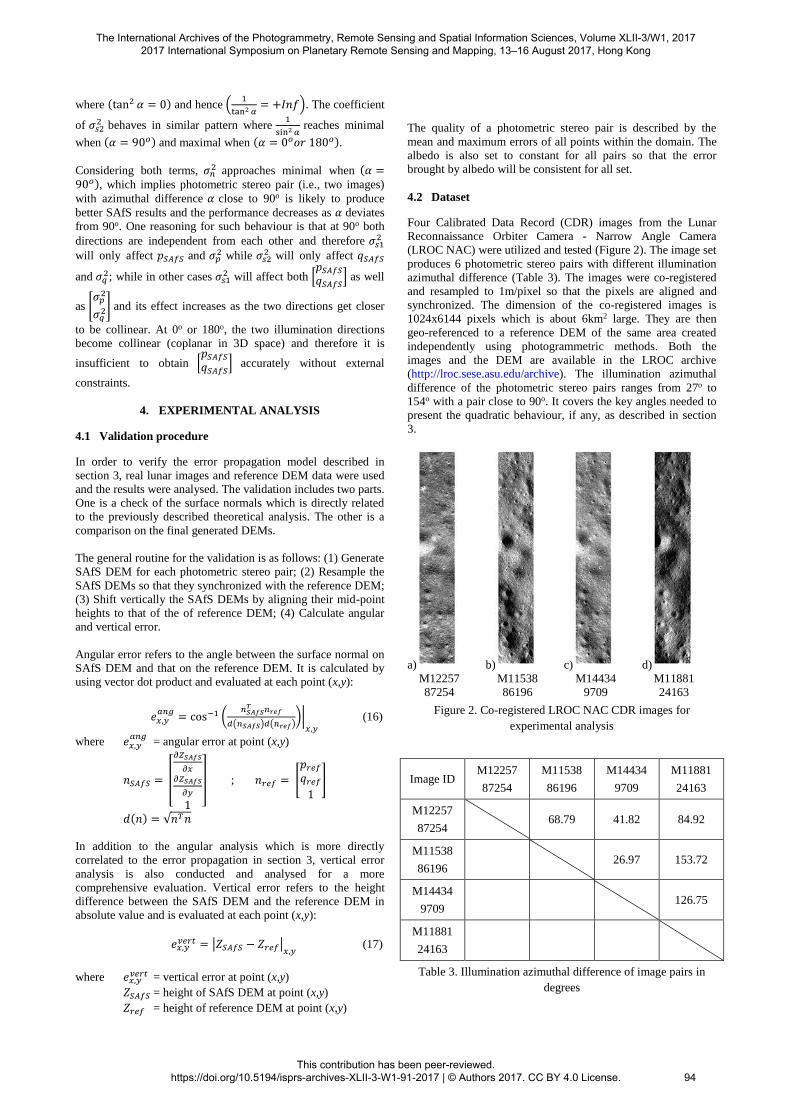
Four Calibrated Data Record (CDR) images from the Lunar

Reconnaissance Orbiter Camera - Narrow Angle Camera

(LROC NAC) were utilized and tested (Figure 2). The image set

produces 6 photometric stereo pairs with different illumination

azimuthal difference (Table 3). The images were co-registered

and resampled to 1m/pixel so that the pixels are aligned and

synchronized. The dimension of the co-registered images is

1024x6144 pixels which is about 6km2 large. They are then

geo-referenced to a reference DEM of the same area created

independently using photogrammetric methods. Both the

images and the DEM are available in the LROC archive

(http://lroc.sese.asu.edu/archive). The illumination azimuthal

difference of the photometric stereo pairs ranges from 27o to

154o with a pair close to 90o. It covers the key angles needed to

present the quadratic behaviour, if any, as described in section

3.

a) b) c) d)

M12257

87254

M11538

86196

M14434

9709

M11881

24163

Figure 2. Co-registered LROC NAC CDR images for

experimental analysis

Image ID M12257

87254

M11538

86196

M14434

9709

M11881

24163

M12257

87254 68.79 41.82 84.92

M11538

86196 26.97 153.72

M14434

9709 126.75

M11881

24163

Table 3. Illumination azimuthal difference of image pairs in

degrees



94

http://lroc.sese.asu.edu/archive

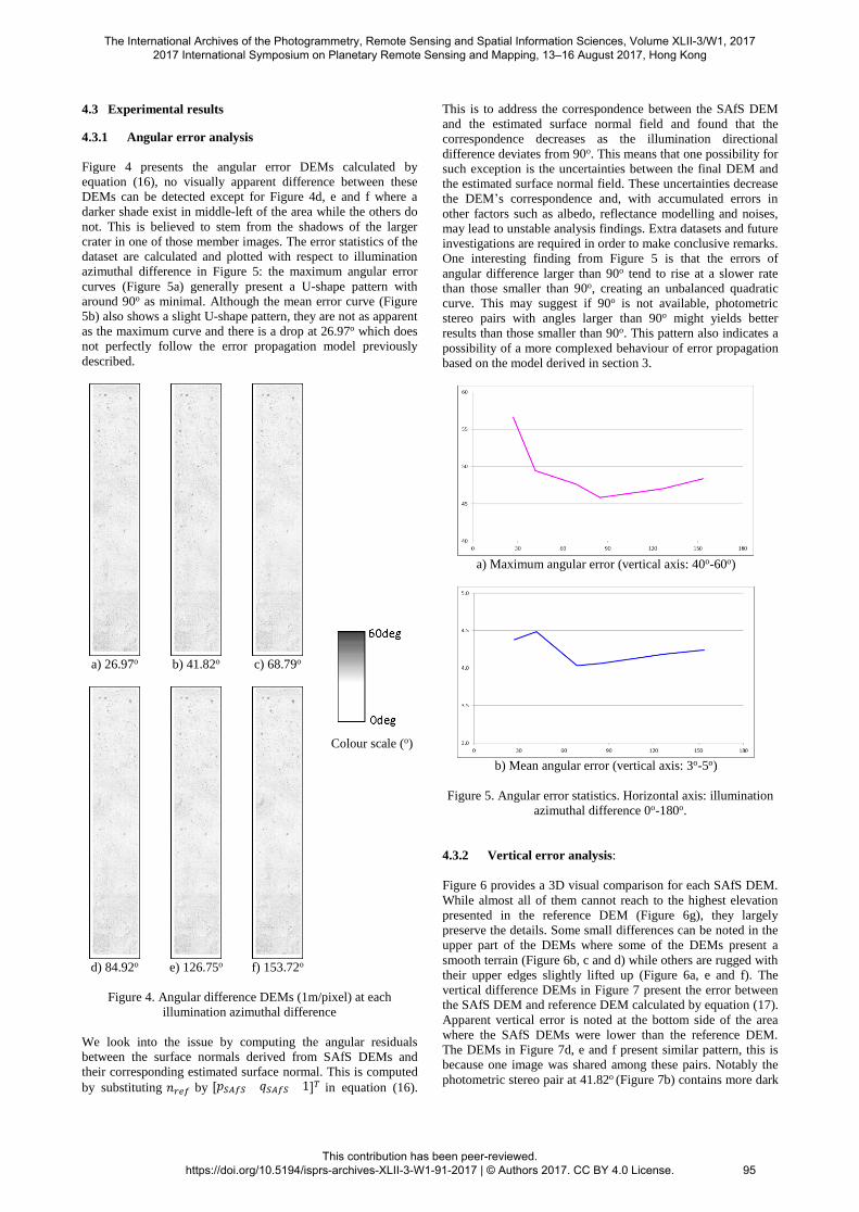
4.3 Experimental results

4.3.1 Angular error analysis

Figure 4 presents the angular error DEMs calculated by

equation (16), no visually apparent difference between these

DEMs can be detected except for Figure 4d, e and f where a

darker shade exist in middle-left of the area while the others do

not. This is believed to stem from the shadows of the larger

crater in one of those member images. The error statistics of the

dataset are calculated and plotted with respect to illumination

azimuthal difference in Figure 5: the maximum angular error

curves (Figure 5a) generally present a U-shape pattern with

around 90o as minimal. Although the mean error curve (Figure

5b) also shows a slight U-shape pattern, they are not as apparent

as the maximum curve and there is a drop at 26.97o which does

not perfectly follow the error propagation model previously

described.

a) 26.97o

b) 41.82o

c) 68.79o

Colour scale (o)

d) 84.92o

e) 126.75o

f) 153.72o

Figure 4. Angular difference DEMs (1m/pixel) at each

illumination azimuthal difference

We look into the issue by computing the angular residuals

between the surface normals derived from SAfS DEMs and

their corresponding estimated surface normal. This is computed

by substituting 𝑛𝑟𝑒𝑓 by [𝑝𝑆𝐴𝑓𝑆 𝑞𝑆𝐴𝑓𝑆 1]𝑇 in equation (16).

This is to address the correspondence between the SAfS DEM

and the estimated surface normal field and found that the

correspondence decreases as the illumination directional

difference deviates from 90o. This means that one possibility for

such exception is the uncertainties between the final DEM and

the estimated surface normal field. These uncertainties decrease

the DEM’s correspondence and, with accumulated errors in

other factors such as albedo, reflectance modelling and noises,

may lead to unstable analysis findings. Extra datasets and future

investigations are required in order to make conclusive remarks.

One interesting finding from Figure 5 is that the errors of

angular difference larger than 90o tend to rise at a slower rate

than those smaller than 90o, creating an unbalanced quadratic

curve. This may suggest if 90o is not available, photometric

stereo pairs with angles larger than 90o might yields better

results than those smaller than 90o. This pattern also indicates a

possibility of a more complexed behaviour of error propagation

based on the model derived in section 3.

a) Maximum angular error (vertical axis: 40o-60o)

b) Mean angular error (vertical axis: 3o-5o)

Figure 5. Angular error statistics. Horizontal axis: illumination

azimuthal difference 0o-180o.

4.3.2 Vertical error analysis:

Figure 6 provides a 3D visual comparison for each SAfS DEM.

While almost all of them cannot reach to the highest elevation

presented in the reference DEM (Figure 6g), they largely

preserve the details. Some small differences can be noted in the

upper part of the DEMs where some of the DEMs present a

smooth terrain (Figure 6b, c and d) while others are rugged with

their upper edges slightly lifted up (Figure 6a, e and f). The

vertical difference DEMs in Figure 7 present the error between

the SAfS DEM and reference DEM calculated by equation (17).

Apparent vertical error is noted at the bottom side of the area

where the SAfS DEMs were lower than the reference DEM.

The DEMs in Figure 7d, e and f present similar pattern, this is

because one image was shared among these pairs. Notably the

photometric stereo pair at 41.82o (Figure 7b) contains more dark



95

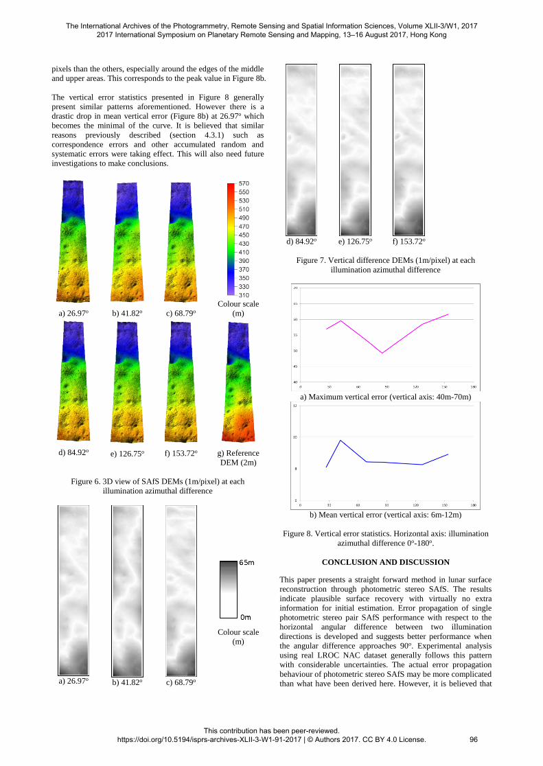
pixels than the others, especially around the edges of the middle

and upper areas. This corresponds to the peak value in Figure 8b.

The vertical error statistics presented in Figure 8 generally

present similar patterns aforementioned. However there is a

drastic drop in mean vertical error (Figure 8b) at 26.97o which

becomes the minimal of the curve. It is believed that similar

reasons previously described (section 4.3.1) such as

correspondence errors and other accumulated random and

systematic errors were taking effect. This will also need future

investigations to make conclusions.

a) 26.97o

b) 41.82o

c) 68.79o

Colour scale

(m)

d) 84.92o

e) 126.75o

f) 153.72o

g) Reference

DEM (2m)

Figure 6. 3D view of SAfS DEMs (1m/pixel) at each


a) 26.97o

b) 41.82o

c) 68.79o

Colour scale

(m)

d) 84.92o

e) 126.75o

f) 153.72o

Figure 7. Vertical difference DEMs (1m/pixel) at each


a) Maximum vertical error (vertical axis: 40m-70m)

b) Mean vertical error (vertical axis: 6m-12m)

Figure 8. Vertical error statistics. Horizontal axis: illumination

azimuthal difference 0o-180o.

CONCLUSION AND DISCUSSION

This paper presents a straight forward method in lunar surface

reconstruction through photometric stereo SAfS. The results

indicate plausible surface recovery with virtually no extra

information for initial estimation. Error propagation of single

photometric stereo pair SAfS performance with respect to the

horizontal angular difference between two illumination

directions is developed and suggests better performance when

the angular difference approaches 90o. Experimental analysis

using real LROC NAC dataset generally follows this pattern

with considerable uncertainties. The actual error propagation

behaviour of photometric stereo SAfS may be more complicated

than what have been derived here. However, it is believed that



96

the error propagation model described here provides the basic

structure for future derivation of more sophisticated models.

ACKNOWLEDGEMENTS

The work was supported by a grant from the Research Grants

Council of Hong Kong (Project No: PolyU 152086/15E) and a

grant from the National Natural Science Foundation of China

(Project No: 41471345).

REFERENCES

Capanna, C., Gesquière, G., Jorda, L., Lamy, P., Vibert, D.,

2013. Three-dimensional reconstruction using multiresolution

photoclinometry by deformation. The Visual Computer, 29(6-8),

pp. 825-835.

Frankot, R. T., Chellappa, R., 1988. A Method for Enforcing

Integrability in Shape from Shading Algorithms. IEEE

Transactions on Pattern Analysis and Machine Intelligence,

10(4), pp. 439-451.

Grumpe, A., Belkhir, F., Wöhler, C., 2014. Construction of

lunar DEMs based on reflectance modelling. Advances in Space

Research, 53(12), pp. 1735-1767.

Horn, B. K. P., 1977. Understanding Image Intensities.

Artificial Intelligence, 8(2), pp. 201-231.

Horn, B. K. P., 1990. Height and Gradient from Shading.

International Journal of Computer Vision, 5(1), pp. 37-75.

Hapke, B., 2002. Bidirectional Reflectance Spectroscopy. 5.

The Coherent Backscatter Opposition Effect and Anisotropic

Scattering. Icarus, 157(2002), pp. 523-534.

Lohse, V., Heipke, C., 2004. Multi-image Shape-from-shading:

Derivation of Planetary Digital Terrain Models Using

Clementine Images. The International Archives of the

Photogrammetry, 35(B4), pp. 828-833.

McEwen, A. S., 1991. Photometric Functions for

Photoclinometry and Other Applications. Icarus, 92(1991), pp.

298-311.

Woodham, R. J., 1980. Photometric method for determining

surface orientation from multiple images. Optical Engineering,

19(1), pp. 139-144.

Wu, B., Liu, W.C., Grumpe, A., Wöhler, C., 2017. Construction

of Pixel-Level Resolution DEMs from Monocular Images by

Shape and Albedo from Shading Constrained with Low-

Resolution DEM. ISPRS Journal of Photogrammetry and

Remote Sensing, doi: 10.1016/j.isprsjprs.2017.03.007.


This contribution has been peer-reviewed. https://doi.org/10.5194/isprs-archives-XLII-3-W1-91-2017 | © Authors 2017. CC BY 4.0 License. 97

Documents

PHOTOMETRIC STEREO SHAPE-AND-ALBEDO … · PHOTOMETRIC STEREO SHAPE-AND-ALBEDO-FROM-SHADING FOR PIXEL-LEVEL RESOLUTION LUNAR SURFACE RECONSTRUCTION Wai Chung Liu, Bo Wu* Dept. of