arX

iv:1

308.

0507

v1 [

mat

h.N

A]

2 A

ug 2

013

Uniformly accurate numerical schemes for highly oscillatory

Klein-Gordon and nonlinear Schrodinger equations

Philippe Chartier ∗ Nicolas Crouseilles † Mohammed Lemou ‡

Florian Mehats §

August 16, 2018

Abstract

This work is devoted to the numerical simulation of nonlinear Schrodinger andKlein-Gordon equations. We present a general strategy to construct numerical schemeswhich are uniformly accurate with respect to the oscillation frequency. This is astronger feature than the usual so called “Asymptotic preserving” property, the lastbeing also satisfied by our scheme in the highly oscillatory limit. Our strategy enablesto simulate the oscillatory problem without using any mesh or time step refinement,and the orders of our schemes are preserved uniformly in all regimes. In other words,since our numerical method is not based on the derivation and the simulation ofasymptotic models, it works in the regime where the solution does not oscillate rapidly,in the highly oscillatory limit regime, and in the intermediate regime with the sameorder of accuracy. In the same spirit as in [5], the method is based on two mainingredients. First, we embed our problem in a suitable “two-scale” reformulation withthe introduction of an additional variable. Then a link is made with classical strategiesbased on Chapman-Enskog expansions in kinetic theory despite the dispersive contextof the targeted equations, allowing to separate the fast time scale from the slow one.Uniformly accurate (UA) schemes are eventually derived from this new formulationand their properties and performances are assessed both theoretically and numerically.

Contents

1 Introduction 2

2 Two-scale formulation of the oscillatory equation 42.1 Setting of the problem . . . . . . . . . . . . . . . . . . . . . . . . . . . . . . 42.2 Bounds in Hσ of the solution of the transport equation . . . . . . . . . . . 52.3 A formal Chapman-Enskog expansion . . . . . . . . . . . . . . . . . . . . . 62.4 Estimates of time derivatives . . . . . . . . . . . . . . . . . . . . . . . . . . 8

∗INRIA-Rennes Bretagne Atlantique, IPSO Project†INRIA-Rennes Bretagne Atlantique, IPSO Project‡CNRS and IRMAR, Universite de Rennes 1 and INRIA-Rennes Bretagne Atlantique, IPSO Project§IRMAR, Universite de Rennes 1 and INRIA-Rennes Bretagne Atlantique, IPSO Project

1

3 First order scheme 113.1 Local truncation error . . . . . . . . . . . . . . . . . . . . . . . . . . . . . . 133.2 Global error . . . . . . . . . . . . . . . . . . . . . . . . . . . . . . . . . . . . 143.3 Choice of the initial data for the first order scheme . . . . . . . . . . . . . . 15

4 A second order scheme 154.1 Local truncation error . . . . . . . . . . . . . . . . . . . . . . . . . . . . . . 164.2 Global error . . . . . . . . . . . . . . . . . . . . . . . . . . . . . . . . . . . . 184.3 Choice of the initial data for the second order scheme . . . . . . . . . . . . 20

5 Applications and numerical results 215.1 The nonlinear Klein-Gordon equation in the nonrelativistic limit regime . . 215.2 The nonlinear Schrodinger equation in a highly oscillatory regime . . . . . . 31

1 Introduction

This work is concerned with the numerical solution of highly-oscillatory differential equa-tions in an infinite dimensional setting. Our main two applications here are the nonlinearSchrodinger equation and the nonlinear Klein-Gordon equation, although, prior to ad-dressing them specifically, we envisage the more general situation of an abstract differen-tial equation in a Hilbert space. To be a bit more specific, we shall consider equations ofthe form

d

dtuε(t) = F(t, t/ε, uε(t)), t ∈ [0, T ], uε(0) = u0, (1.1)

where the vector field (t, τ, u) 7→ F(t, τ, u) is supposed to be periodic of period P withrespect to the variable τ (we shall denote T ≡ R/(PZ)). The parameter ε is supposedto have a positive real value in an interval of the form ]0, ε0] for some ε0 > 0. However,ε is not necessarily vanishing and may be as well thought of as being close to 1: thismeans we can consider equation (1.1) simultaneously in different regimes, namely highly-oscillatory for small values of ε or smooth for larger values of ε, and our aim is to designa versatile numerical method, capable of handling these two extreme regimes as much asall intermediate ones.

Generally speaking, standard numerical methods for equation (1.1) exhibit errors ofthe form ∆tp/εq for some positive p and q. The user of such methods is thus forced torestrict the step-size ∆t to values less than εq/p in order to obtain some accuracy. Thisbecomes an unacceptable constraint for vanishing values of ε. Whenever equation (1.1)admits a limit model, Asymptotic-Preserving (AP) schemes [10] have been designed toovercome this restriction: the methods we construct obey the corresponding requirement,i.e. they degenerate into a consistent numerical scheme for the limit model whenever εtends to zero.

As favorable as this property may seem, the error behavior of an AP scheme may dete-riorate for “intermediate” regimes where ε is neither very small nor large. The derivationof asymptotic models for (1.1) has been the subject of many works – see e.g. [3, 4, 15, 16]for time-averaging techniques and [1, 8, 14] for homogenization techniques – and a hierar-chy of averaged vector fields and models at different orders of ε can be classically written

2

from asymptotic expansions of the solution. However, these asymptotic models are validonly when ε is small enough and any numerical methods based on the direct approxima-tion of such averaged vector fields introduce a truncation index n and a correspondingincompressible error εn.

In sharp contrast, our strategy in this paper consists in developing numerical schemesthat solve directly (1.1) for a wide range of ε-values with uniform accuracy. The mainoutput of our work are numerical methods for highly oscillatory equations of type (1.1),which are uniformly accurate (UA) with respect to the parameter ε ∈]0, ε0], ε0 > 0. Thesemethods, as we shall demonstrate, are able to capture the various scales occurring in thesystem, while keeping numerical parameters (for instance ∆t) independent of the degreeof stiffness (ε).

The main idea underlying our strategy (see also [5]) consists in separating the two timescales naturally present in (1.1), namely the slow time t and the fast time t/ε. To thisaim, we embed the solution uε into a two-variable function (t, τ) ∈ [0, T ] × T 7→ U ε(t, τ)while imposing that U ε coincides with uε on the diagonal τ = t/ε. Clearly, this impliesthat

d

dtuε(t) = ∂tU

ε(t, t/ε) +1

ε∂τU

ε(t, t/ε) = F(t, t/ε, U ε(t, t/ε)).

By virtue of the “separation” principle, we then consider the equation over the whole(t, τ)-domain, i.e.

∂tUε(t, τ) +

1

ε∂τU

ε(t, τ) = F(t, τ, U ε(t, τ)). (1.2)

An observation of paramount importance is that no initial condition for (1.2) is evident,since only the value U ε(0, 0) = u0 is prescribed: consequently, as such, the transportequation (1.2) is not a Cauchy problem and may have many solutions. This apparentobstacle is in fact the way out to our numerical difficulties: given that for any smoothinitial condition U ε(0, τ) = U ε

0 (τ) satisfying U ε0 (0) = u0, we can recover the solution uε

from the values of U ε on the diagonal τ = t/ε, the missing Cauchy condition should beregarded as an additional degree of freedom.

Now, it turns out that for some specific choice of U ε0 , it is possible to prove that

U ε and its time-derivatives are bounded on [0, T ] × T uniformly w.r.t. ε. The pointis, in this two-scale formulation (1.2) of (1.1), that stiffness is confined in the sole term1ε∂τU

ε. Interpreting this singularly perturbed term as a “collision” operator, we can derivethe asymptotic behavior of U ε through a Chapman-Enskog expansion (see for instance[6]) from which averaged models (first and second order) can easily be obtained. Theinitial datum U ε

0 is then chosen so as to satisfy this expansion at t = 0, a requirementcompatible with U ε

0 (0) = u0. Two numerical schemes are then proposed for this augmentedproblem, following the strategy in [5]. In the present work, these schemes are proved to beuniformly accurate with respect to ε: they have respectively orders 1 and 2 uniformly inε. These properties are assessed by numerical experiments on the nonlinear Klein-Gordonand Schrodinger equations.

This paper is organized as follows. In Section 2.1, we present the two-scale formulationin a general framework and perform in Subsection 2.3 the Chapman-Enskog expansion ofU ε. The question of the choice of the initial datum U ε(0, τ) for this augmented equation

3

(1.2) is addressed. In Section 3, a first-order numerical scheme is introduced and analyzedwhile a second-order one is similarly studied in Section 4. Finally, Section 5 is devoted toa series of numerical tests which confirm the theoretical properties of our schemes whenapplied to the Schrodinger and Klein-Gordon equations and demonstrate the relevance ofour strategy.

2 Two-scale formulation of the oscillatory equation

In this section, we formulate and analyze the equation obtained by decoupling the slowvariable t and the fast one τ = t/ε.

2.1 Setting of the problem

Given ε0 > 0, we consider the following highly-oscillatory evolution problem

∂tuε = F(t, t/ε, uε), t ≥ 0, ε ∈]0, ε0], uε(0) = u0, (2.1)

where the unknown t 7→ uε(t) is a smooth map onto a Sobolev space Hs (either Hs(Tdx)

or Hs(Rd) with d ≥ 1) and the vector-field (t, τ, u) 7→ F(t, τ, u) ∈ Hs is a smooth map,P -periodic w.r.t. τ ∈ T (T ≡ R/PZ). Let us emphasize that F may also depend on ε,although we shall not reflect specifically this dependence: whenever this is the case, allbounds on F and its derivatives then implicitly hold uniformly in ε. In order to work inBanach algebras, we require that s > d/2 + 8, a condition whose necessity will becomeapparent for the numerical schemes.

As described in the Introduction section, we envisage uε(t) as the diagonal solution ofthe following transport equation which constitutes our starting point:

∂tUε +

1

ε∂τU

ε = F(t, τ, U ε), U ε(0, τ) = U ε0 (τ), (2.2)

where the unknown is now the function (t, τ) 7→ U ε(t, τ) ∈ Hs. The choice of the Cauchycondition U ε

0 (τ) is discussed below, but it is already clear that uε(t) and U ε(t, t/ε) coincideprovided that U ε

0 (0) = u0.For our purpose, we shall need that the vector field F obeys the following assumption,

where each derivation w.r.t. t or τ typically costs 2 derivatives in the space variable.Indeed, for applications to nonlinear Klein-Gordon or Schrodinger equation – see (5.7)and (5.12) –, one has in mind vector fields of the form

F(t, τ, U ε) = f(eit∆U ε, eiτ∆U ε

),

where f is a smooth function.

Assumption (A) For all α ∈ {0 · · · 3}, β ∈ {0, 1} and γ ∈ {0 · · · 3}, for all s, σ such that

s ≥ σ > 2(α + β) + d/2, the functional ∂αt ∂βτ ∂

γuF is continuous and locally bounded from

R+ × T×Hs toL(Hσ × . . .×Hσ

︸ ︷︷ ︸γ times

,Hσ−2(α+β)).

4

2.2 Bounds in Hσ of the solution of the transport equation

Similar related transport equations will occur in our analysis, with possibly other functionsthan F and initial conditions with various regularities. A somehow preliminary result thusconcerns the existence and uniqueness of the solution of the general Cauchy problem

∂tΦε +

1

ε∂τΦ

ε = G(t, τ,Φε), Φε(0, τ) = Φε0(τ) ∈ Hσ, (2.3)

where Φε0 (possibly) depends on ε ∈]0, ε0] and is assumed to be not identically zero.

Proposition 2.1 Let T > 0, let σ > d/2 and suppose that G is a locally Lipschitz con-tinuous map from [0, T ]×T×Hσ into Hσ, that it admits derivatives ∂τG and ∂uG whichare continuous and locally bounded from [0, T ] × T × Hσ into, respectively, Hσ−2 andL(Hσ−2,Hσ−2). If Φε

0 ∈ C0(T;Hσ)∩C1(T;Hσ−2) is uniformly bounded in ε ∈]0, ε0] withrespect to the L∞

τ (Hσ) norm then, for any κ > 1, there exists 0 < Tκ ≤ T such that forall ε ∈]0, ε0], equation (2.3) has a unique solution Φε ∈ C0([0, Tκ]× T;Hσ) and we have

∀t ∈ [0, Tκ], supε∈]0,ε0]

‖Φε(t, ·)‖L∞τ (Hσ) ≤ κ sup

ε∈]0,ε0]‖Φε

0(·)‖L∞τ (Hσ). (2.4)

Moreover, Φε has first derivatives w.r.t. both t and τ which are functions of C0([0, Tκ]×T;Hσ−2). If in addition, G satisfies the estimate

∀(t, τ) ∈ [0, T ]× T, ∀v ∈ Hσ, ‖G(t, τ, v)‖Hσ ≤ CG‖v‖Hσ +DG

for some positive constants CG and DG, then equation (2.3) has a unique solution inC0([0, T ] × T;Hσ) satisfying

∀t ∈ [0, T ], supε∈]0,ε0]

‖Φε(t, ·)‖L∞τ (Hσ) ≤ ( sup

ε∈]0,ε0]‖Φε

0(·)‖L∞τ (Hσ) +DGt)e

tCG .

Proof. Considering a smooth solution Φε(t, τ) of (2.3) and denoting ϕε(t, τ) = Φε(t, τ +t/ε), it is easy to check that

∂tϕε(t, τ) = ∂tΦ

ε(t, τ + t/ε) +1

ε∂τΦ

ε(t, τ + t/ε) = G(t, τ + t/ε, ϕε(t, τ)),

so that the smooth function t 7→ ϕε(t, τ), parametrized by (τ, ε) ∈ T×]0, ε0], is thensolution of the ordinary differential equation

∂tϕε(t, τ) = G(t, τ + t/ε, ϕε(t, τ)), ϕε(0, τ) = Φε

0(τ). (2.5)

According to Cauchy-Lipschitz theorem in Hσ (a Banach space), equation (2.5) has aunique maximal solution on an interval of the form [0, T ε

max[ (when 0 < T εmax < T ) or a

solution on [0, T ], which furthermore satisfies the following inequality

‖ϕε(t, τ)‖Hσ ≤ ‖Φε0(τ)‖Hσ +

∫ t

0‖G(θ, τ + θ/ε, ϕε(θ, τ)‖Hσdθ.

DenoteR = sup

ε∈]0,ε0]‖Φε

0(τ)‖Hσ

5

andMκ = sup{‖G(t, τ, u)‖Hσ , 0 ≤ t ≤ T, τ ∈ T, ‖u‖Hσ ≤ κR}.

Now, as long as ‖ϕε(t, τ)‖Hσ ≤ R, we have

‖ϕε(t, τ)‖Hσ ≤ ‖Φε0(τ)‖Hσ + tMκ,

so that

T εmax ≥ Tκ := min

(T,

(κ− 1)R

Mκ

)> 0

and estimate (2.4) holds. Now, since ∂τG (resp. ∂uG) is a continuous and locally boundedfunction from [0, T ]×T×Hσ toHσ−2 (resp. to L(Hσ−2,Hσ−2)), then ψε(t, τ) := ∂τϕ

ε(t, τ)is the unique solution on [0, Tκ] of the linear differential equation in Hσ−2

∂tψε(t, τ) = (∂τG)(t, τ + t/ε, ϕε(t, τ)) + ∂uG(t, τ + t/ε, ϕε(t, τ))ψε(t, τ),

ψε(0, τ) = ∂τΦε0(τ) ∈ Hσ−2.

Hence ϕε has first derivatives ∂tϕε in Hσ and ∂τϕ

ε in Hσ−2. Finally, since Φε(t, τ) =ϕε(t, τ − t/ε), we have

∂τΦε(t, τ) = ∂τϕ

ε(t, τ − t/ε) and ∂tΦε(t, τ) = ∂tϕ

ε(t, τ − t/ε)− 1

ε∂τϕ

ε(t, τ − t/ε)

so that Φε has also first derivatives inHσ−2. Finally, the proof of the subsequent assertionsin Proposition 2.1 can be done in the same way, the last estimate being a consequence ofthe Gronwall lemma.

Remark 2.2 From previous formulae, it appears that ∂tΦε exists in Hσ−2 but is not

necessarily uniformly bounded in ε. In order to get a solution Φε with uniformly boundedfirst derivatives, we have to consider an appropriate ε-dependent initial condition Φε

0. Inthe next two subsections, we shall consider a formal expansion of Φε in ε so as to determinehow this initial condition should be prescribed.

2.3 A formal Chapman-Enskog expansion

In this subsection, we analyze formally the behavior of (2.2) in the limit ε → 0 underthe assumption that its solution U ε has uniformly bounded (in ε) derivatives up to order3. Following [5], we thus consider the linear operator L, defined for all periodic (regular)function τ ∈ T 7→ h(τ) by

Lh = ∂τh.

This operator is skew-adjoint with respect to the L2(T) scalar product and its kernel isthe set of constant functions. The L2-projector on this kernel is the averaging operator

Πh :=1

P

∫ P

0h(τ)dτ

which obviously satisfies ΠL ≡ 0. On the set of functions with vanishing average, L isinvertible with inverse defined by

(L−1h)(τ) = (I−Π)

∫ τ

0h(θ)dθ.

6

In order to alleviate notations, we further introduce A := L−1(I − Π) which operates onthe set of periodic functions onto the set of zero-average periodic functions.

The Chapman-Enskog expansion (see for instance [6]) consists in writing the solutionU ε(t, τ) in the form

U ε(t, τ) = Uε(t) + hε(t, τ), (2.6)

whereUε(t) = Π (U ε(t, τ)) , Πhε = 0,

and then, under some regularity assumptions on U ε with respect to t and ε, one seeks thecorrection hε as an expansion in powers of ε:

hε(t, τ) = εh1(t, τ,Uε(t)) + ε2h2(t, τ,U

ε(t)) + . . . . (2.7)

Inserting the decomposition (2.6) into (2.2) leads to

∂tUε + ∂th

ε +1

εLhε = F(t, τ,Uε + hε). (2.8)

Projecting on the kernel of L and taking into account that Πhε = 0, we obtain

∂tUε = Π(F(t, τ,Uε + hε)) , (2.9)

and then subtracting from (2.8)

∂thε +

1

εLhε = (I−Π) (F(t, τ,Uε + hε)) . (2.10)

Since hε belongs to the range of L, we get

hε = εA (F(t, τ,Uε + hε))− εL−1(∂thε). (2.11)

Therefore, provided hε and its first time derivative are uniformly bounded w.r.t. ε, wefirst deduce from this last equation that hε = O(ε). Now if we additionally assume thatthe second and third time derivatives are uniformly bounded w.r.t. ε, then, by a simpleinduction on (2.11), we get

hε(t, τ) = εh1(t, τ,Uε) + ε2h2(t, τ,U

ε) +O(ε3),

with h1 and h2 defined by

h1(t, τ, U) =AF(t, τ, U), (2.12)

h2(t, τ, U) =A∂uF(t, τ, U)AF(t, τ, U) −A2(∂uF(t, τ, U)ΠF(t, τ, U) + ∂tF(t, τ, U)

).

(2.13)

Inserting these corrections into equation (2.9) yields the first and second order averagedmodels

∂tUε = ΠF(t, τ,Uε) +O(ε),

∂tUε = ΠF(t, τ,Uε) + εΠ(∂uF(t, τ,Uε)AF(t, τ,Uε)) +O(ε2).

7

Anticipating on next sections, let us now briefly address the crucial issue of the initialcondition for (2.2). According to the above calculations, one expects to get a smoothsolution of (2.2) if the initial condition U ε

0 follows the same expansion as above, i.e.

U ε0 (τ) = Uε

0 + εAF0(τ,Uε0) (2.14)

+ ε2(A∂uF0(τ,U

ε0)AF0(τ,U

ε0)−A2∂uF0(τ,U

ε0)ΠF0(τ,U

ε0)−A2(∂tF)0(τ,U

ε0))

)

where we have denoted by a subindex 0 the evaluation of functions at t = 0 and whereUε

0 := Uε(0) is chosen so as to be compatible with U ε0 (0) = u0 which is the initial condition

for the original problem (2.1). Starting from Uε0 = u0 + O(ε) and inserting successively

higher-order terms in the previous equation, we can obtain the expression of Uε0 and then

of U ε0 (τ). For instance, we have

Uε0 = u0 + εΠ

∫ τ

0(I−Π)F0(θ, u0)dθ +O(ε2),

so that

U ε0 (τ) = u0 + ε

∫ τ

0(I−Π)F0(θ, u0)dθ +O(ε2)

which provides an initial condition for our first order numerical scheme (see Subsection3.3). The explicit computation of second order terms is postponed to Subsection 4.3.

2.4 Estimates of time derivatives

In this subsection, we indeed prove that the initial condition (2.14) ensures that timederivatives of U ε up to order 3 are uniformly bounded in ε. In the sequel, the followingfunctional space will be useful:

Xσ =⋂

0≤2ℓ<σ−d/2

Cℓ(T;Hσ−2ℓ). (2.15)

Proposition 2.3 Suppose that F satisfies Assumption (A) and let s > d/2+8 and κ > 1.Consider the following initial condition

∀τ ∈ T, U ε(0, τ) = U ε0 (τ) = Uε

0 + (εh1 + ε2h2)(0, τ,Uε0) + ε3rε(τ), (2.16)

where Uε0 ∈ Hs+2 is assumed to be uniformly bounded in ε ∈]0, ε0], where h1 and h2 are

given by (2.12) and (2.13), and where the remainder term rε is assumed to be bounded inXs uniformly in ε. Then the following holds:

(i) U ε0 is uniformly bounded in L∞

τ (Hs) and there exists Tκ > 0 such that, for all ε ∈]0, ε0], equation (2.2), subject to the initial condition (2.16), has a unique solutionU ε(t, τ) ∈ C0([0, Tκ]× T;Hs), which satisfies the uniform bound

∀t ∈ [0, Tκ], supε∈]0,ε0]

‖U ε(t)‖L∞τ (Hs) ≤ κ sup

ε∈]0,ε0]‖U ε

0‖L∞τ (Hs). (2.17)

8

(ii) Moreover, for any Tκ for which (2.17) holds, the solution U ε satisfies the followingestimates

∀t ∈ [0, Tκ], supε∈]0,ε0]

‖∂αt ∂βτ U ε(t)‖L∞τ (Hs−2(α+β)) ≤ C, α = 0, 1, 2, 3, β = 0, 1,

(2.18)for some constant C > 0.

Proof. We prove this proposition in several steps.

Existence of U ε and uniform bound. Let us first estimate the initial condition definedby (2.16). From (2.12), (2.13), one gets

U ε0 = Uε

0 + εAF0 + ε2A∂uF0AF0 − ε2A2∂uF0ΠF0 − ε2A2(∂tF)0 + ε3rε, (2.19)

where, for conciseness, we have further omitted the dependence1 of F0 in τ and Uε0. We

notice that, by Assumption (A), we have

F0, ∂uF0AF0, ∂uF0ΠF0 ∈ Xs+2, and (∂tF)0 ∈ Xs,

with norms uniformly bounded w.r.t. ε. Hence, observing that A and Π are boundedoperators on C0(T;Hσ), for all σ, one deduces that U ε

0 belongs to Xs and is uniformlybounded w.r.t. ε. Hence, according to Proposition 2.1, U ε exists on an interval [0, Tκ]independent of ε, and satisfies

∀0 ≤ t ≤ Tκ, supε∈]0,ε0]

‖U ε(t, ·)‖L∞τ (Hs) ≤ κ sup

ε∈]0,ε0]‖U ε

0 (·)‖L∞τ (Hs).

Furthermore, derivatives of U ε w.r.t. t and τ exist and are functions with values in Hs−2.

Estimate of the first derivative in t. The first derivative V ε = ∂tUε satisfies the

equation

∂tVε +

1

ε∂τV

ε = ∂uF(t, τ, U ε)V ε + ∂tF(t, τ, U ε) (2.20)

with initial condition

V ε0 = F0(U

ε0 )−

1

εLU ε

0 .

From (2.19) and LA = (I−Π), LA2 = A, we obtain

V ε0 = F0(U

ε0 )−F0 +ΠF0 − ε(I−Π)∂uF0AF0 + εA∂uF0ΠF0 + εA(∂tF)0 − ε2Lrε.

Taylor-Lagrange expansions with integral remainder at order one and two give2

F0(Uε0 )−F0 =

∫ 1

0∂uF0(U

ε0 + µ(U ε

0 −Uε0))dµ

(U ε0 −Uε

0

)= OXs(ε)

= ∂uF0(Uε0) (U

ε0 −Uε

0) +

∫ 1

0(1− µ)∂2uF0(U

ε0 + µ(U ε

0 −Uε0))dµ

(U ε0 −Uε

0, Uε0 −Uε

0

)

= ε∂uF0AF0 +OXs(ε2),

1In the sequel, we explicitly mention the dependence F0(Uε0 ) while F0 stands for F(0, τ,Uε

0) and (∂tF)0stands for ∂tF(0, τ,Uε

0).2The notation OXσ is used here for terms uniformly bounded in T with the appropriate Xσ-norm.

9

where we used that rε is uniformly bounded in Xs. Therefore3

V ε0 = ΠF0 +OXs−2(ε) (2.21)

= ΠF0 + ε∂uF0AF0 − ε(I−Π)∂uF0AF0 + εA∂uF0ΠF0 + εA(∂tF)0 +OXs−2(ε2)

= ΠF0 + εΠ∂uF0AF0 + εA∂uF0ΠF0 + εA(∂tF)0 +OXs−2(ε2). (2.22)

In particular, V ε0 ∈ C0(T;Hs−2) ∩ C1(T;Hs−4) and is uniformly bounded in L∞

τ (Hs−2)w.r.t. ε. According to the second part of Proposition 2.1 (for σ = s− 2) with

G(t, τ, V ) = ∂uF(t, τ, U ε(t, τ))V + ∂tF(t, τ, U ε(t, τ))

which is a map from R+ × T×Hs−2 into Hs−2, we thus have an estimate of the form

∀t ∈ [0, Tκ], supε∈]0,ε0]

‖V ε(t, ·)‖L∞τ (Hs−2) ≤

(sup

ε∈]0,ε0]‖V ε

0 (τ)‖L∞τ (Hs−2) +DGTκ

)eTκCG .

Estimate of the second derivative in t. We proceed in an analogous way for W ε =∂2t U

ε = ∂tVε ∈ Hs−4 by considering

∂tWε +

1

ε∂τW

ε =∂2uF(t, τ, U ε)(V ε, V ε) + 2∂t∂uF(t, τ, U ε)V ε

+ ∂2tF(t, τ, U ε) + ∂uF(t, τ, U ε)W ε. (2.23)

The initial condition for W ε can be obtained from (2.20) at t = 0 and (2.22)

W ε0 = −1

εLV ε

0 + ∂uF0(Uε0 )V

ε0 + (∂tF)0(U

ε0 )

= −1

εL(εA∂uF0ΠF0 + εA(∂tF)0

)+ ∂uF0(U

ε0 )V

ε0 + (∂tF)0(U

ε0 ) +OXs−4(ε)

= −(I−Π)∂uF0ΠF0 − (I−Π)(∂tF)0 + ∂uF0ΠF0 + (∂tF)0 +OXs−4(ε)

= Π∂uF0ΠF0 +Π(∂tF)0 +OXs−4(ε), (2.24)

which is uniformly bounded in the Hs−4-norm w.r.t. both ε and τ . By Proposition 2.1applied to W ε(t, τ) with σ = s− 4, one gets that W ε is uniformly bounded in L∞

τ (Hs−4).

Estimate of the third derivative in t. Finally, we derive the equation for Y ε(t, τ) =∂tW

ε(t, τ), which reads

∂tYε +

1

ε∂τY

ε = ∂3uF(t, τ, U ε)(V ε, V ε, V ε) + 3∂t∂2uF(t, τ, U ε)(V ε, V ε)

+ 3∂2uF(t, τ, U ε)(V ε,W ε) + 3∂2t ∂uF(t, τ, U ε)V ε

+ 3∂t∂uF(t, τ, U ε)W ε + ∂3tF(t, τ, U ε) + ∂uF(t, τ, U ε)Y ε. (2.25)

We then extract Y ε0 (τ) = ∂tW

ε(0, τ) from (2.23):

Y ε0 = −1

εLW ε

0 + ∂2uF0(Uε0 )(V

ε0 , V

ε0 ) + 2(∂t∂uF)0(U

ε0 )V

ε0 + (∂2t F)0(U

ε0 ) + ∂uF0(U

ε0 )W

ε0 .

The only source of concern could come from the term in factor of 1ε . However, it is clear

from the expression (2.24) of W ε0 that LW ε

0 = OXs−6(ε), so that

Y ε0 = OXs−6(1), (2.26)

3Notice that LXσ is continuously embedded in Xσ−2.

10

and according to Proposition 2.1, Y ε(t, τ) is thus uniformly bounded in τ and ε in theHs−6-norm, since the source-term ∂3tF(t, τ, U ε) is uniformly bounded in Hs−6.

Estimate of derivatives in τ . Using equation (2.2) on U ε, (2.20) on V ε and (2.23) onW ε, we have

∂τUε = ε(−∂tU ε + F(t, τ, U ε) = ε(−V ε + F(t, τ, U ε),

∂τVε = ε(−∂tV ε + ∂uF(t, τ, U ε)V ε) = ε(−W ε + ∂uF(t, τ, U ε)V ε),

∂τWε = ε(−∂tW ε + ∂2uF(t, τ, U ε)(V ε, V ε)

+ 2∂t∂uF(t, τ, U ε)V ε + ∂2tF(t, τ, U ε) + ∂uF(t, τ, U ε)W ε).

Since the terms in the parentheses of the right-hand sides are uniformly bounded in (t, τ, ε)respectively in Hs−2, Hs−4 and Hs−6 using Assumption (A), we deduce that ∂τU

ε =OHs−2(ε), ∂τV

ε = OHs−4(ε), and ∂τWε = OHs−6(ε). The estimate of ∂τY

ε = ∂3t ∂τUε

from (2.25) however requires some additional argument since Zε = ∂tYε is not necessarily

uniformly bounded. We thus consider the equation satisfied by Zε = ∂τYε obtained by

differentiation w.r.t. to τ of equation (2.25). This equation is of the form

∂tZε +

1

ε∂τ Z

ε = S(t, τ, U ε, V ε,W ε, Y ε, ∂τUε, ∂τV

ε, ∂τWε) + ∂uF(t, τ, U ε)Zε,

and its initial condition can be obtained by differentiating Y ε0 w.r.t. τ , leading to Zε

0 =OXs−8(1) and hence, once again by Proposition 2.1, Zε is uniformly bounded in L∞

τ (Hs−8),since the source-term S lies in C0([0, Tκ]× T;Hs−8).

Remark 2.4 If in Proposition 2.3 we modify the hypotheses as follows: s > d/2 + 4 andwe assume the following initial condition

∀τ ∈ T, U ε(0, τ) = U ε0 (τ) = Uε

0 + εh1(0, τ,Uε0) + ε2rε(τ), (2.27)

where Uε0 ∈ Hs is uniformly bounded in ε, where h1 is given by (2.12), and where the

remainder term rε is assumed to be bounded in Xs uniformly in ε, then the conclusionsof this Proposition are modified as follows: Item (i) is unchanged, and (ii) is replaced by:

(ii) For any Tκ for which (2.17) holds, the solution U ε satisfies the following estimates

∀t ∈ [0, Tκ], supε∈]0,ε0]

‖∂αt U ε(t)‖L∞τ (Hs−2α) ≤ C, α = 0, 1, 2, (2.28)

for some constant C > 0.

3 First order scheme

This section is devoted to the construction and the numerical analysis of a first ordernumerical scheme. We only focus on the time discretization, and the other variable τ iskept at the continuous level. We thus define a uniform grid tn = n∆t of a time interval[0, Tκ], n = 0, 1, ..., N, with N∆t = Tκ (recall that [0, Tκ] is the interval of time on whichthe solution U ε of (2.2) is well-defined irrespectively of ε) and consider the following

11

numerical scheme for this equation. Denoting U εn ≈ U ε(tn, τ) and U

εn+1 ≈ U ε(tn+1, τ), it

advances the solution from time tn to time tn+1 through the inductive equation

U εn+1(τ) = U ε

n(τ) + ∆tF(tn, τ, Uεn(τ)) −

∆t

ε∂τU

εn+1(τ). (3.1)

This scheme does not define U εn+1 in a unique way, unless we impose – assuming that

U εn is periodic with period P – that U ε

n+1 is periodic with the same period. Under thisrequirement, pre-multiplying (3.1) by eµτ with µ = ε

∆t , we have

∂τ (eµτU ε

n+1) = µeµτ (U εn+1 +

1

µ∂τU

εn+1) = µeµτ (U ε

n +∆tF(tn, τ, Uεn))

so that, upon integrating from τ to τ + P , we obtain

(eµP − 1)eµτU εn+1(τ) = µ

∫ τ+P

τeµθ

(U εn(θ) + ∆tF(tn, θ, U

εn(θ))

)dθ,

or in more concise manner

U εn+1(τ) =

µ

exp(µP )− 1

∫ τ+P

τeµ(θ−τ)

(U εn(θ) + ∆tF(tn, θ, U

εn(θ))

)dθ. (3.2)

Note that it is straightforward to check that U εn+1, as given by formula (3.2), is periodic of

period P . This last equation defines precisely the scheme whose convergence we now wishto investigate. From previous computations, we observe that the operator Qµ = I + 1

µ∂τplay a central role. We thus briefly study its properties in the following proposition.

Proposition 3.1 Let σ ∈ R. The operator Qµ, defined from the set C1(T;Hσ) ontoC0(T;Hσ) by

∀τ ∈ T, (Qµg)(τ) = g(τ) +1

µ(∂τg)(τ)

is invertible and its inverse, which is defined on C0(T;Hσ) with values in C1(T;Hσ), canbe explicitly written as

∀τ ∈ T, (Q−1µ g)(τ) =

µ

exp(µP )− 1

∫ τ+P

τeµ(θ−τ)g(θ)dθ.

Moreover, it satisfies the following estimate:

∀g ∈ C0(T;Hσ), ‖Q−1µ g‖L∞

τ (Hσ) ≤ ‖g‖L∞τ (Hσ)

Proof. The inversion formula has been proven above. As for the estimate, it stems fromthe identity

µ

exp(µP )− 1

∫ τ+P

τeµ(θ−τ)dθ = 1.

12

3.1 Local truncation error

Proposition 3.2 Let s > d/2+4, κ > 1 and Uε0 uniformly bounded in Hs with respect to

ε. Consider U ε the solution of equation (2.2) with initial condition (2.27), and fix ∆t = Tκ

Nfor some N ∈ N

∗. The consistency error ℓeεn+1 for the numerical scheme (3.1) or (3.2),defined for n = 0, . . . , N − 1 by

ℓeεn+1 := U ε(tn+1)− U εn+1 (3.3)

where(QµU

εn+1)(·) = U ε(tn, ·) + ∆tF(tn, ·, U ε(tn, ·))

satisfies the following estimate

supε∈]0,ε0]

‖ℓeεn+1‖L∞τ (Hs−4) ≤ C∆t2 (3.4)

for some positive error constant C.

Proof. In the sequel, we shall omit the variable τ unless explicitly needed, as it playsessentially no role in subsequent computations. From the equation satisfied by U ε(t, τ)(see (2.2)), we have

QµUε(tn+1) = U ε(tn+1) + ∆t

(F(tn+1, U

ε(tn+1))− ∂tUε(tn+1)

),

so thatQµ(ℓe

εn+1) = gn, (3.5)

with

gn := U ε(tn+1)− U ε(tn) + ∆t(F(tn+1, U

ε(tn+1))−F(tn, Uε(tn))− ∂tU

ε(tn+1)).

By Taylor expansion (with integral remainder) at t = tn+1 we get, on the one hand,

U ε(tn)− U ε(tn+1) = (−∆t)∂tUε(tn+1) +

∫ tn

tn+1

(tn − t)∂2t Uε(t)dt,

and on the other hand,

F(tn+1, Uε(tn+1)) = F(tn, U

ε(tn)) +

∫ tn+1

tn

(∂tF(t, U ε(t)) + ∂uF(t, U ε(t))∂tU

ε(t))dt,

so that

gn = ∆t

∫ tn+1

tn

(∂tF(t, U ε(t)) + ∂uF(t, U ε(t))∂tU

ε(t) +(tn − t)

∆t∂2tU

ε(t))dt.

According to Remark 2.4 and the Assumption (A) on F , the quantities supt∈[0,Tκ] ‖∂αt U ε‖L∞τ (Hs−2α), α =

0, 1, 2 are uniformly bounded in ε, so that

supε∈]0,ε0]

‖gn‖L∞τ (Hs−4) ≤ C∆t2, (3.6)

and by Proposition 3.1, we get the desired estimate.

13

3.2 Global error

Theorem 3.3 Let s > d/2 + 4, κ > 1 and Uε0 uniformly bounded in Hs with respect to

ε. Let U ε be the unique solution of (2.2) on [0, Tκ] subject to the initial condition (2.27),and let (U ε

n)0≤n≤N be defined for all τ ∈ T by (3.2) with U ε0 again defined by (2.27). Then

there exists ∆t0 > 0 and C > 0 such that the following estimate holds

∀∆t < ∆t0, supε∈]0,ε0]

‖U ε(tn)− U εn‖L∞

τ (Hs−4) ≤ C∆t, (3.7)

for all n = 0, . . . , N , where Tκ = N∆t is the final time.

Proof. The global error eεn+1 := U ε(tn+1)− U εn+1 can be decomposed into two parts

eεn+1 =(U ε(tn+1)− U ε

n+1

)

︸ ︷︷ ︸local error ℓeεn+1

+(U εn+1 − U ε

n+1

)

︸ ︷︷ ︸transported error teεn+1

whereQµU

εn = U ε(tn) + ∆tF(tn, U

ε(tn)).

We haveQµe

εn+1 = Qµℓe

εn+1 +Qµte

εn+1

with (see equation (3.5))Qµℓe

εn+1 = gn

andQµte

εn+1 = eεn +∆t

(F(tn, U

ε(tn))−F(tn, Uεn)).

Let R > 0 be fixed. As long as supε∈]0,ε0] ‖eεn‖L∞τ (Hs−4) < R (recall that eε0 = 0), we have

for λ ∈ [0, 1]

‖λU εn + (1− λ)U ε(tn)‖L∞

τ (Hs−4) ≤ ‖U ε(tn)‖L∞τ (Hs−4) + λ‖eεn‖L∞

τ (Hs−4) ≤ C0 +R

independently of ε, where we used the uniform bound on U ε given in Remark 2.4. Thenwe can use the local bound of ∂uF provided by Assumption (A) in order to obtain

‖F(tn, Uεn)−F(tn, U

ε(tn))‖L∞τ (Hs−4) ≤

∫ 1

0

∥∥∥∂uF(tn, λUεn + (1− λ)U ε(tn))e

εn

∥∥∥L∞τ (Hs−4)

dλ

≤ C1‖eεn‖L∞τ (Hs−4).

Finally, using estimate (3.4) of Proposition 3.2 and Proposition 3.1, we have

‖eεn+1‖L∞τ (Hs−4) ≤ (1 + C1∆t)‖eεn‖L∞

τ (Hs−4) + C2∆t2

and a discrete Gronwall lemma provides us with the bound

‖eεn+1‖L∞τ (Hs−4) ≤

C2∆t

C1(exp(C1Tκ)− 1).

By induction, we can a posteriori verify that ‖eεn‖Hs−4 < R for all n = 0, · · · , N , provided∆t < ∆t0 with ∆t0 := RC1 e

−C1Tκ /C2. This completes the proof.

14

3.3 Choice of the initial data for the first order scheme

So far, we have addressed the question of numerical approximation of the augmentedproblem (2.2), subject to an initial condition U ε

0 (τ) satisfying (2.27). We now come backto our original problem (2.1), and recall that if U ε

0 (0) = u0, then uε(t) can be recovered

as the diagonal uε(t) = U ε(t, t/ε), so the global estimate (3.7) yields

∀∆t < ∆t0, supε∈]0,ε0]

‖uε(tn)− U εn(tn/ε)‖Hs−4 ≤ C∆t.

In practice, if the only known initial data is u0, we proceed as follows to construct asuitable associated initial data U ε

0 . We set

U ε0 (τ) := u0 + εh1(0, τ, u0)− εh1(0, 0, u0) = u0 + ε

∫ τ

0(I−Π)F0(θ, u0)dθ, (3.8)

and

Uε0 := ΠU ε

0 = u0 + εΠ

∫ τ

0(I−Π)F0(θ, u0)dθ.

In the numerical Section 5, this choice of initial data will be referred to as first order initialdata. Then, (2.27) is satisfied if the remainder term is defined by

rε(τ) :=1

ε2(U ε

0 (τ)−Uε0 − εh1(0, τ,U

ε0)) =

1

ε(h1(0, τ, u0)− h1(0, τ,U

ε0)) .

From Assumption (A), it is easy to prove that, as soon as u0 ∈ Hs, the function Uε0 and r

ε

are uniformly bounded respectively in Hs and Xs (this space is defined by (2.15)), whichis enough to apply Theorem 3.3.

4 A second order scheme

We now present a two-stage second order scheme. The first stage is composed of half-a-stepof the first-order scheme presented in previous section:

U εn+1/2 = U ε

n +∆t

2F(tn, U

εn)−

∆t

2ε∂τU

εn+1/2, (4.1)

while the second stage computes the updated approximation U εn+1 as follows:

U εn+1 = U ε

n +∆tF(tn+1/2, Uεn+1/2)−

∆t

2ε∂τ (U

εn + U ε

n+1). (4.2)

As in the previous section, a more concise version of the scheme reads

Q2µUεn+1/2 = U ε

n +∆t

2F(tn, U

εn), (4.3)

Q2µUεn+1 = (2I−Q2µ)U

εn +∆tF(tn+1/2, U

εn+1/2). (4.4)

Prior to proving our main result, we state an elementary result which is an essentialingredient of subsequent proofs.

15

Lemma 4.1 Consider a function g ∈ L2(T;Hσ) with σ ∈ R. The following estimateshold true for the operator Qµ defined in Proposition 3.1:

∀β ∈ [−1, 1], ‖((1 + β)Q−1µ − βI)g‖L2

τ (Hσ) ≤ ‖g‖L2

τ (Hσ), (4.5)

with equality for |β| = 1, and

‖∂τQ−1µ g‖L2

τ (Hσ) ≤ 2µ‖g‖L2

τ (Hσ). (4.6)

Proof. Let g ∈ L2(T;Hσ) and ((1 + β)Q−1µ − βI)g = f . This last equality is clearly

equivalent to

g − f =1

µ∂τ (βg + f).

Taking the inner product against βg + f in the real Hilbert space L2τ (H

σ) and using theskew-symmetry of ∂τ , we get

‖f‖2L2τ (H

σ) − β‖g‖2L2τ (H

σ) = (1− β)〈f, g〉L2τ (H

σ) ≤ (1− β)‖f‖L2τ (H

σ)‖g‖L2τ (H

σ).

This proves the case of equality in (4.5) and also implies

(‖f‖L2τ (H

σ) + β‖g‖L2τ (H

σ))(‖f‖L2τ (H

σ) − ‖g‖L2τ (H

σ)) ≤ 0,

which ends the proof of inequality (4.5). To prove (4.6), we simply remark that

∂τQ−1µ g = µ(g −Q−1

µ g),

and use (4.5) with β = 0.

4.1 Local truncation error

Proposition 4.2 Let s > d/2 + 8, κ > 1 and Uε0 uniformly bounded in Hs+2 with respect

to ε. Consider U ε the solution of equation (2.2) with initial condition (2.16) given byProposition 2.3, and fix ∆t = Tκ

N for some N ∈ N∗. The local truncation error ℓen+1 for

the scheme (4.1)-(4.2) defined for n = 0, . . . , N − 1 by ℓeεn+1 := U ε(tn+1)− U εn+1 where

Q2µUεn+1/2 = U ε(tn) +

∆t

2F(tn, U

ε(tn)),

Q2µUεn+1 = (2I−Q2µ)U

ε(tn) + ∆tF(tn+1/2, Uεn+1/2),

satisfies the following estimates

supε∈]0,ε0]

‖ℓeεn+1‖L∞τ (Hs−4−2k) ≤ C(∆t)2+k, (4.7)

andsup

ε∈]0,ε0]‖∂τ ℓeεn+1‖L∞

τ (Hs−6−2k) ≤ C(∆t)2+k, (4.8)

for k ∈ {0, 1} and for some positive error constant C.

16

Proof. From the equation satisfied by U ε(t, τ) at tn and tn+1 we have

(2I−Q2µ)Uε(tn) = U ε(tn)−

∆t

2

(F(tn, U

ε(tn))− ∂tUε(tn)

),

Q2µUε(tn+1) = U ε(tn+1) +

∆t

2

(F(tn+1, U

ε(tn+1))− ∂tUε(tn+1)

)

so that(Q2µℓe

εn+1) = gn

with

gn := U ε(tn+1)− U ε(tn) +∆t

2

(F(tn+1, U

ε(tn+1)) + F(tn, Uε(tn))− 2F(tn+1/2, U

εn+1/2)

)

− ∆t

2

(∂tU

ε(tn+1) + ∂tUε(tn)

). (4.9)

Now, by a symmetric Taylor expansion, it is straightforward to show that

U ε(tn+1)− U ε(tn) =∆t

2

(∂tU

ε(tn+1) + ∂tUε(tn)

)+Rn,

with

Rn :=1

2

∫ tn+1

tn

(tn − t)(tn+1 − t)∂3t Uε(t)dt.

This remainder term can be estimated in two different ways. First, using the uniformbound of ‖∂3t U ε‖L∞

τ (Hs−6) in (2.18), we get directly

‖Rn‖L∞τ (Hs−6) ≤ C∆t3.

Second, integrating by parts Rn = 12

∫ tn+1

tn(tn+ tn+1−2t)∂2t U

ε(t)dt, and using the uniform

bound of ‖∂2t U ε‖L∞τ (Hs−4) in (2.18), we obtain

‖Rn‖L∞τ (Hs−4) ≤ C∆t2.

Here and in the sequel, C denotes a generic positive constant independent of ε ∈]0, ε0].Next, from the proof of Proposition 3.2, we have the estimate

‖U εn+1/2 − U ε(tn+1/2)‖L∞

τ (Hs−4) ≤ C∆t2

from which we get

‖F(tn+1/2, Uε(tn+1/2))−F(tn+1/2, U

εn+1/2)‖L∞

τ (Hs−4) ≤ C∆t2,

where we have used the local boundedness of ∂uF and the uniform boundedness of U ε.Using once more a Taylor expansion (of the function t 7→ F(t, U ε(t)) around t = tn+1/2), itstems from the local boundedness of the first and second derivatives of F , and the uniformboundedness of the first and second time derivatives of U ε,

‖F(tn+1, Uε(tn+1)) + F(tn, U

ε(tn))− 2F(tn+1/2, Uε(tn+1/2))‖L∞

τ (Hs−4) ≤ C∆t2.

This eventually leads to

supε∈]0,ε0]

‖gn‖L∞τ (Hs−4−2k) ≤ C∆t3 + sup

ε∈]0,ε0]‖Rn‖L∞

τ (Hs−4−2k) ≤ C(∆t)2+k

for k ∈ {0, 1}. The estimate (4.7) then follows from the properties of the inversion formulafor Q2µ.

17

The estimate (4.8) can be obtained in a similar way. Denoting

G(t, τ, U ε, V ε) = ∂τF(t, τ, U ε) + ∂uF(t, τ, U ε)V ε,

we see that the derivative w.r.t. τ of the scheme (4.3), (4.4) yields the following schemeon the unknown V ε = ∂τU

ε:

Q2µVεn+1/2 = V ε

n +∆t

2G(tn, U ε

n, Vεn ),

Q2µVεn+1 = (2I−Q2µ)V

εn +∆tG(tn+1/2, U

εn+1/2, V

εn+1/2).

The only difference is now that the r.h.s. G is a now a map from R+ × T × Hs−2 intoHs−2 which has, according to Proposition 2.3, uniformly bounded derivatives ∂αt G for theL∞t,τ (H

s−2(α+1)) norm for α = 0, 1, 2, 3.

4.2 Global error

Theorem 4.3 Let s > d/2 + 8, κ > 1 and Uε0 uniformly bounded in Hs+2 with respect to

ε. Let U ε be the unique solution of (2.2) on [0, Tκ] subject to the initial condition (2.16)given by Proposition 2.3, and let (U ε

n)0≤n≤N be defined for all τ ∈ T by (4.3) with U ε0 again

defined by (2.16). Then there exists ∆t0 > 0 and C > 0 such that the following estimateholds

∀∆t < ∆t0, supε∈]0,ε0]

‖U ε(tn)− U εn‖L∞

τ (Hs−8) ≤ C∆t2, (4.10)

for all n = 0, . . . , N , where Tκ = N∆t is the final time.

Proof. Let R > 0 and let us assume for the time being, that eεn satisfies the uniformestimate

supε∈]0,ε0]

‖eεn‖L∞τ (Hs−6) ≤ R, (4.11)

for all n ≤ N , so that all terms like ∂uF(t, ·, λU ε(tn, ·) + (1 − λ)U εn(·)) are also uniformly

bounded from Assumption (A) and Proposition 2.3. This hypothesis can eventually bejustified by induction as in Theorem 3.3, using (4.15) that we will obtained in the midstof the proof.

The global error eεn+1 = U ε(tn+1)− U εn+1 can be decomposed into two parts as

eεn+1 =(U ε(tn+1)− U ε

n+1

)

︸ ︷︷ ︸local error ℓeεn+1

+(U εn+1 − U ε

n+1

),

︸ ︷︷ ︸transported error teεn+1

where

Q2µUεn+1/2 = U ε(tn) +

∆t

2F(tn, U

ε(tn)),

Q2µUεn+1 = (2I−Q2µ)U

ε(tn) + ∆tF(tn+1/2, Uεn+1/2).

We thus haveQ2µe

εn+1 = Q2µℓe

εn+1 +Q2µte

εn+1

withQ2µℓe

εn+1 = gn ,

18

gn being still defined by (4.9), and

Q2µteεn+1 =

(2I−Q2µ

)eεn +∆t

(F(tn+1/2, U

εn+1/2)−F(tn+1/2, U

εn+1/2)

). (4.12)

Step 1: second order estimate of the global error in L2τ (H

s−6). In this first step,we prove the following estimate on the global error:

∀∆t < ∆t0, supε∈]0,ε0]

‖eεn‖L2τ (H

s−6) ≤ C∆t2. (4.13)

The second term of the r.h.s. of (4.12) can be bounded as follows∥∥∥F(tn+1/2, U

εn+1/2)−F(tn+1/2, U

εn+1/2)

∥∥∥L2τ (H

s−6)

=∥∥∥∫ 1

0∂uF

(tn+1/2, λU

εn+1/2 + (1− λ)U ε

n+1/2

)(U εn+1/2 − U ε

n+1/2

)dλ

∥∥∥L2τ (H

s−6)

≤ C1‖eεn+1/2‖L2τ (H

s−6)

where eεn+1/2 = U εn+1/2 − U ε

n+1/2 can also be bounded by using the properties of Q−12µ

(Lemma 4.1 for β = 0)

‖eεn+1/2‖L2τ (H

s−6) ≤ (1 + C2∆t)‖eεn‖L2τ (H

s−6). (4.14)

Using inequality (4.5) in Lemma 4.1 for β = 0 and β = 1, together with the local errorestimate (4.7) established above, we finally have

‖eεn+1‖L2τ (H

s−6) ≤(1 + C1∆t(1 + C2∆t)

)‖eεn‖L2

τ (Hs−6) + C3∆t

3

and owing to a discrete version of Gronwall lemma, we end up with a L2 estimate for eεn

‖eεn‖L2τ (H

s−6) ≤ C∆t2.

Step 2: first order estimate of the global error in L∞τ (Hs−6). In this second step,

we prove:∀∆t < ∆t0, sup

ε∈]0,ε0]‖eεn‖L∞

τ (Hs−6) ≤ C∆t. (4.15)

To this aim, we estimate ∂τ eεn in L2

τ (Hs−6). Using (4.5) for β = 1 (remarking that Q−1

2µ

and ∂τ commute) and (4.6), we deduce from (4.12) that

‖∂τ teεn+1‖L2τ (H

s−6) ≤ ‖∂τ eεn‖L2τ (H

s−6) + 4µ∆tC1(1 +C2∆t)‖eεn‖L2τ (H

s−6).

Therefore, since µ = ε/∆t, we deduce from (4.13), from the local truncation error (4.8)(with k = 0) and, again, from Lemma 4.1 that

‖∂τ eεn+1‖L2τ (H

s−6) ≤ ‖∂τ eεn‖L2τ (H

s−6) + C∆t2,

which gives directly (4.15) after summation and after using the Sobolev embedding ofH1

τ (Hs−6) into L∞

τ (Hs−6).At this stage, we can already ensure that (4.11) is satisfied, provided that ∆t < ∆t0

with ∆t0 := R/C, the constant C being given in (4.15).

Step 3: second order estimate of the global error in L∞τ (Hs−8). The last step of the

proof consists in proving the same estimate as (4.13) for ∂τeεn, but in L

2τ (H

s−8). This proof

19

is similar as Step 1, up to replacing the vector field F(t, U) by G(t, U, V ) = ∂τF(t, U) +∂uF(t, U)V and the local truncation error (4.7) by (4.8) (with k = 1). Therefore, we pointout the following estimate on G. If U , U belong to a bounded set of L∞

τ (Hs−6) and if V ,V belong to a bounded set of L2

τ (Hs−8), then, for all t,

∥∥∥G(t, U , V )− G(t, U, V )∥∥∥L2τ (H

s−8)

≤∥∥∥∂τF(t, U )− ∂τF(t, U)

∥∥∥L2τ (H

s−8)+

∥∥∥∂uF(t, U)V − ∂uF(t, U)V∥∥∥L2τ (H

s−8)

≤ C‖U − U‖L2τ (H

s−8) +∥∥∥(∂uF(t, U )− ∂uF(t, U))V

∥∥∥L2τ (H

s−8)+

∥∥∥∂uF(t, U)(V − V )∥∥∥L2τ (H

s−8)

≤ C‖U − U‖L2τ (H

s−8) + C‖U − U‖L∞τ (Hs−8)‖V ‖L2

τ (Hs−8) + C‖V − V ‖L2

τ (Hs−8)

≤ C‖U − U‖L2τ (H

s−8) + C‖∂τ U − ∂τU‖L2τ (H

s−8) + C‖V − V ‖L2τ (H

s−8),

where the Sobolev embedding of H1τ (H

s−8) into L∞τ (Hs−8) has been used for the last

inequality. With U = U εn+1/2, U = U ε

n+1/2, V = ∂τ Uεn+1/2, V = ∂τU

εn+1/2 and using (4.14)

and (4.13), we have∥∥∥G(t, U , V )− G(t, U, V )

∥∥∥L2τ (H

s−8)≤ C∆t2 +C‖∂τ eεn+1/2‖L2

τ (Hs−8).

Arguing like in Step 1, we deduce that ‖∂τ eεn+1‖L2τ (H

s−8) ≤ (1+C∆t)‖∂τ eεn‖L2τ (H

s−8)+C∆t3

and we finally conclude that

supε∈]0,ε0]

‖eεn‖H1τ (H

s−8) ≤ C∆t2.

The Sobolev embedding of H1τ (H

s−8) into L∞τ (Hs−8) allows again to obtain the desired

error estimatesup

ε∈]0,ε0]‖eεn‖L∞

τ (Hs−8) ≤ C∆t2.

4.3 Choice of the initial data for the second order scheme

As in Subsection 3.3, let us explain our strategy to construct the initial condition U ε0 (τ)

for the augmented problem (2.2), as soon as the initial condition u0 for (2.1) is known.We set4

U ε0 (τ) :=u0 + εh1(τ, u0)− εh1(0, u0) + ε2h2(τ, u0)− ε2h2(0, u0)

− ε2∂uh1(τ, u0)h1(0, u0) + ε2∂uh1(0, u0)h1(0, u0), (4.16)

where h1 and h2 are defined by (2.12) and (2.13), and

Uε0 := ΠU ε

0 = u0 − εh1(0, u0)− ε2h2(0, u0) + ε2∂uh1(0, u0)h1(0, u0).

In the numerical Section 5, this choice of initial data will be referred to as second orderinitial data. Assuming that u0 ∈ Hs+4, one deduces from Assumption (A) that Uε

0 is

4For simplicity, we omit here the t dependency in h1 and h2 which are all evaluated at t = 0.

20

uniformly bounded in Hs+2. Next, consider the remainder term defined according to(2.16) by

rε(τ) :=1

ε3(U ε0 (τ)−Uε

0 − εh1(τ,Uε0)− ε2h2(τ,U

ε0)).

By Taylor expansions, one gets

rε(τ) =1

ε2(h1(τ, u0)− ε∂uh1(τ, u0)h1(0, u0)− h1(τ,U

ε0) + εh2(τ, u0)− εh2(τ,U

ε0))

=1

ε2(h1(τ, u0)− ε∂uh1(τ, u0)h1(0, u0)− h1(τ, u0 − εh1(0, u0)) +OXs(ε2)

)

= OXs(1).

The above choice of initial data ensures the validity of the assumptions of Theorem 4.3.

5 Applications and numerical results

In this section, we apply our two-scale technique in two situations. We first presentnumerical experiments for the nonlinear Klein-Gordon equation in the nonrelativistic limitregime, then we consider a stiffer problem, the nonlinear Schrodinger equation in a highlyoscillatory regime.

A special care will be given to the choice of the initial condition U ε0 (τ) for the aug-

mented problem, that will be constructed from the initial condition u0. The possiblechoices will be:

– the uncorrected initial data U ε0 = u0,

– the first order initial data U ε0 given by (3.8),

– the second order initial data U ε0 given by (4.16),

– a third order initial data U ε0 obtained by pushing the Chapman-Enskog expansion of

Subsection 2.3 to the order three.

5.1 The nonlinear Klein-Gordon equation in the nonrelativistic limit

regime

In this subsection, we consider the following nonlinear Klein-Gordon (NKG) equation:

ε∂ttu−∆u+1

εu+ f(u) = 0, x ∈ R

d, t > 0, (5.1)

with initial conditions given as

u(0, x) = φ(x), ∂tu(0, x) =1

εγ(x), x ∈ R

d. (5.2)

The unknown is the function u(t, x) : R1+d → C and the parameter ε > 0 is inversely

proportional to the square of the speed of light. The nonlinearity is assumed to be a smoothfunction f satisfying f(0) = 0, f(R) ⊂ R and the gauge invariance f(eisu) = eisf(u) for

21

all u ∈ C, s ∈ R. This implies in particular that f satisfies f(z) = f(z) for all z ∈ C.The limit ε → 0 in equation (5.1), (5.2), referred to as the nonrelativistic limit, has beenstudied in [11, 12, 13]. The regime of small ε (but not zero) is highly oscillatory and hasbeen recently explored numerically in [2] by Gauschi-type exponential methods, allowingfor time steps of order O(ε). In [7], a different approach is proposed, based on asymptoticexpansions with respect to ε. None of these methods is uniformly accurate in ε ∈ (0, 1].We apply here our two-scale reformulation technique which naturally leads to uniformlyaccurate numerical schemes.

It is convenient to rewrite (5.1) under the equivalent form of a first order system intime (see e.g. [13, 7]). Setting

v+ = u− iε(1 − ε∆)−1/2∂tu, v− = u− iε(1 − ε∆)−1/2∂tu, (5.3)

and denoting

f(v+, v−) =

(f(

1

2(v+ + v−)) , f(

1

2(v+ + v−))

),

we obtain that (5.1), (5.2) is equivalent to the following system on the unknown v =(v+, v−):

i∂tv = −1

ε(1− ε∆)1/2v − (1− ε∆)−1/2f(v), (5.4)

v(0, ·) = (v+(0, ·), v−(0, ·)) =(φ− i(1− ε∆)−1/2∂tγ , φ− i(1 − ε∆)−1/2∂tγ

). (5.5)

Finally, introducing the filtered unknown

u = e−i tε

√1−ε∆v,

we obtain the following equation:

∂tu = i(1− ε∆)−1/2e−i tε

√1−ε∆f

(ei

tε

√1−ε∆u

). (5.6)

Note that (5.6) is under the form (2.1) if we set

F(t, τ, u, ε) = i(1− ε∆)−1/2e−iτe−itAε f(eiτ eitAεu

)(5.7)

with

Aε =1

ε

(√1− ε∆− 1

).

This self-adjoint operator is not singular as ε→ 0: for all ε > 0, we have

0 ≤ Aε ≤ −1

2∆

in the sense of operators. It can be checked that this vector field F satisfies Assumption(A).

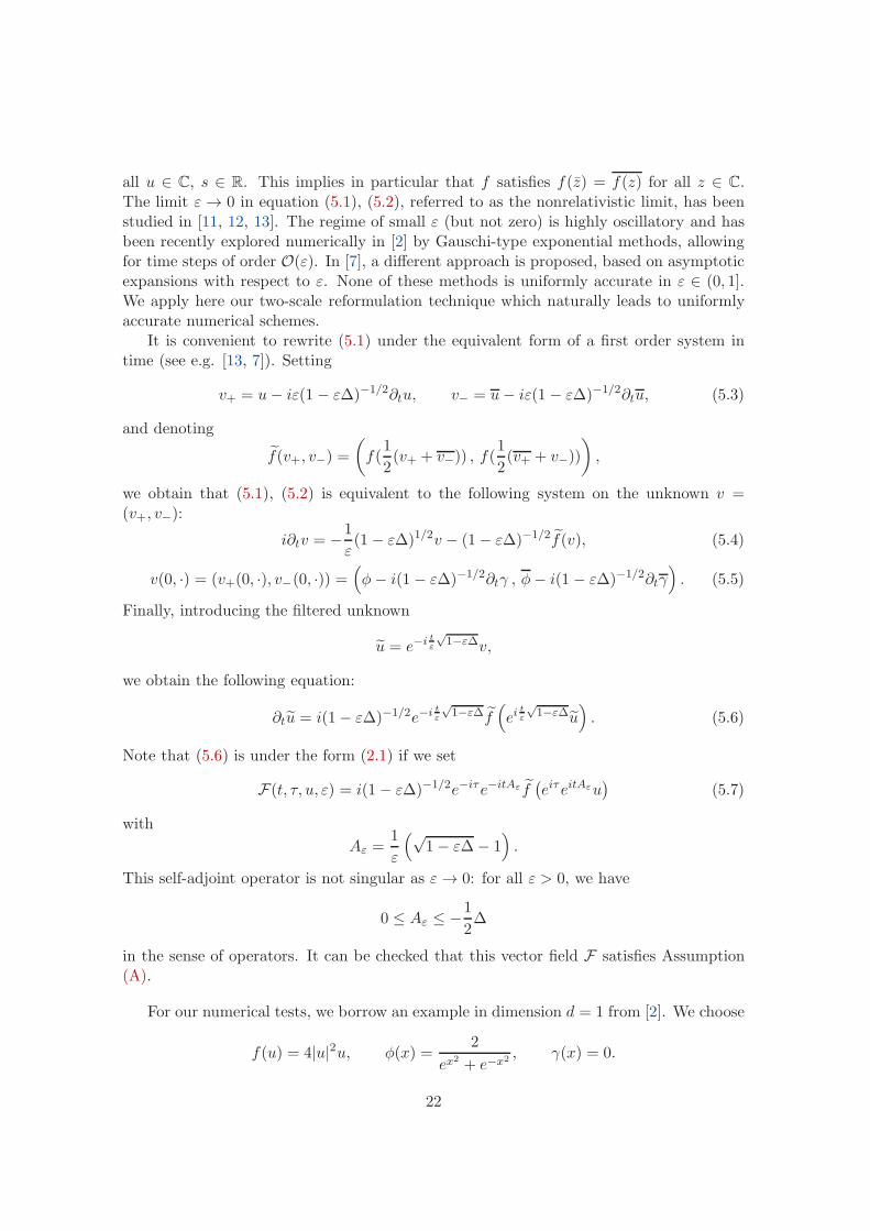
For our numerical tests, we borrow an example in dimension d = 1 from [2]. We choose

f(u) = 4|u|2u, φ(x) =2

ex2 + e−x2 , γ(x) = 0.

22

The final time of the simulations is Tf = 0.4. The computational domain in x is [−8, 8]and is large enough for periodic boundary conditions to be taken, with no significativeerror compared to the solution in the whole space (this feature is a posteriori checked).For the numerical evaluations of the function F in our scheme, a spectral method is usedin the x variable and the fast Fourier transform is used in the practical implementation.For the series of tests, the reference solution is computed as follows. For ε ≥ 10−2,we use the Yoshida fourth order splitting method [17] with ∆x = 16/256 = 0.0625,∆t = ε Tf/2000. For smaller values of ε, we rather use our second order uniformly accuratescheme, with small grid steps: ∆x = 16/256 = 0.0625, ∆t = 2π/512000 ≈ 1.2 × 10−5,∆τ = 2π/128 ≈ 0.05. We shall use the Hs relative error of a given numerical schemewhich we define as

Es =‖uref (tfinal, ·) − unum(tfinal, ·)‖Hs

‖uref (tfinal, ·)‖Hs

, (5.8)

where unum(tfinal, ·) is the approximated solution obtained by the considered numericalscheme, at the final time tfinal of the simulation. In order to validate the referencesolution and show the behavior of a non uniformly accurate scheme, we first compare thereference solution uref (tfinal, x) to the numerical solution uStrang(tfinal, x) computed withthe following Strang splitting algorithm for (5.4):

– Step 1 for t ∈ [tn, tn + ∆t2 ]: we solve

i∂tv1 = −1

ε(1 − ε∆)1/2v1, v1|t=tn = vn

which has an explicit solution in the Fourier space.

– Step 2 for t ∈ [tn, tn +∆t]: we solve

i∂tv2 = −(1− ε∆)−1/2f(v2), v2|t=tn = v1|t=tn+∆t2

which has also an explicit solution (remark indeed that the solution v2 = (v2+, v2−) of thisequation satisfies v2+ + v2− =constant).

– Step 3 for t ∈ [tn + ∆t2 , tn +∆t]: we solve

i∂tv3 = −1

ε(1− ε∆)1/2v3, , v3|t=tn+

∆t2

= v2|t=tn+∆t

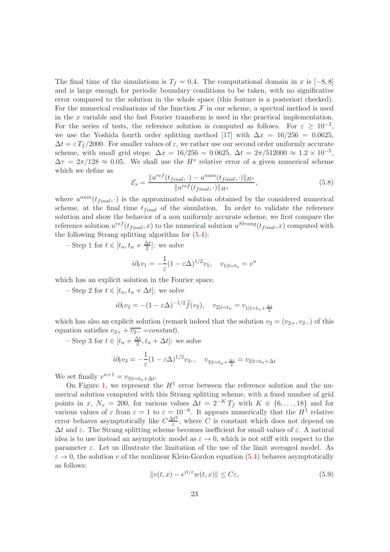
We set finally vn+1 = v3|t=tn+∆t.On Figure 1, we represent the H1 error between the reference solution and the nu-

merical solution computed with this Strang splitting scheme, with a fixed number of gridpoints in x, Nx = 200, for various values ∆t = 2−K Tf with K ∈ {6, . . . , 18} and forvarious values of ε from ε = 1 to ε = 10−6. It appears numerically that the H1 relativeerror behaves asymptotically like C∆t2

ε , where C is constant which does not depend on∆t and ε. The Strang splitting scheme becomes inefficient for small values of ε. A naturalidea is to use instead an asymptotic model as ε→ 0, which is not stiff with respect to theparameter ε. Let us illustrate the limitation of the use of the limit averaged model. Asε→ 0, the solution v of the nonlinear Klein-Gordon equation (5.4) behaves asymptoticallyas follows:

‖v(t, x) − eit/εw(t, x)‖ ≤ Cε, (5.9)

23

10−6

10−5

10−4

10−3

10−2

10−12

10−10

10−8

10−6

10−4

10−2

Delta t

H1 e

rror

Slope 2

ε=1ε=0.1ε=0.01ε=0,001ε=0,0001ε=0,00001

(a) Error with respect to ∆t

10−6

10−4

10−2

100

10−15

10−10

10−5

100

105

epsilon

H1 e

rror

∆ t=2−6 Tf

∆ t=2−7 Tf

∆ t=2−8 Tf

∆ t=2−9 Tf

∆ t=2−10 Tf

∆ t=2−11 Tf

∆ t=2−12 Tf

∆ t=2−13 Tf

∆ t=2−14 Tf

∆ t=2−15 Tf

∆ t=2−16 Tf

∆ t=2−17 Tf

∆ t=2−18 Tf

(b) Error with respect to ε

Figure 1: (NKG) H1 relative error (in log-log scale)for the Strang splitting scheme.

where w solves the averaged equation

i∂tw = −1

2∆w +

1

2π

∫ 2π

0e−iτ f

(eiτw

)dτ. (5.10)

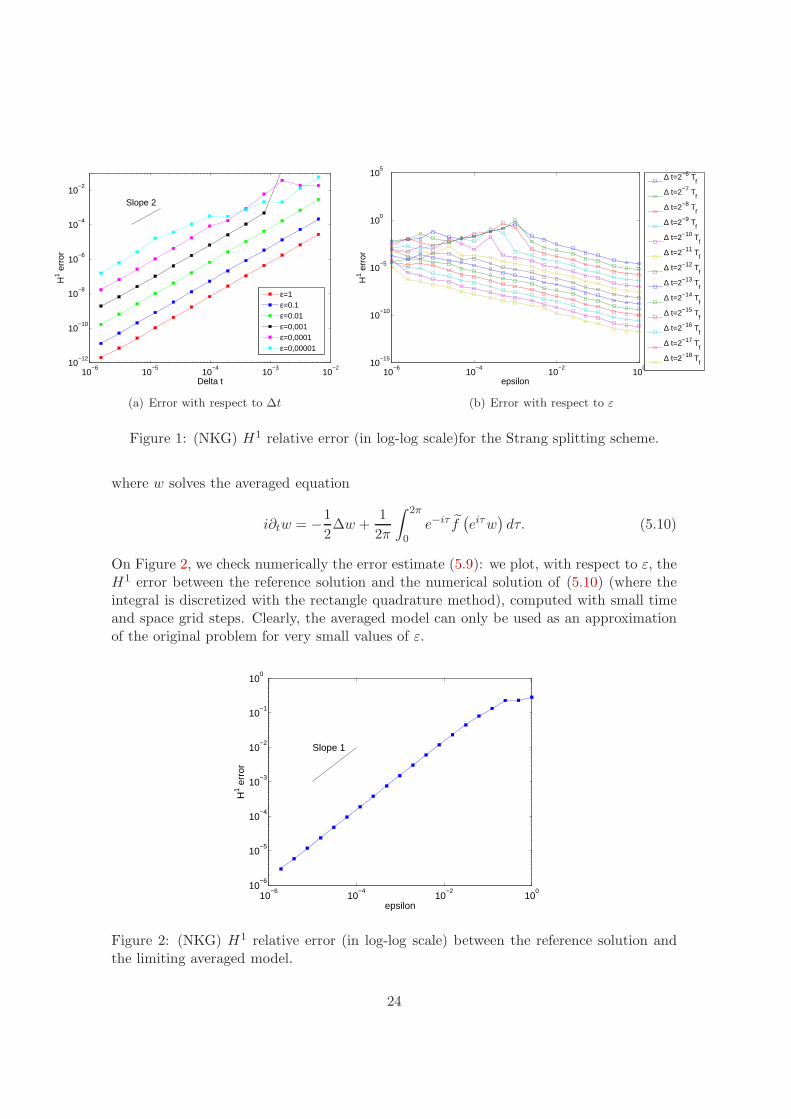
On Figure 2, we check numerically the error estimate (5.9): we plot, with respect to ε, theH1 error between the reference solution and the numerical solution of (5.10) (where theintegral is discretized with the rectangle quadrature method), computed with small timeand space grid steps. Clearly, the averaged model can only be used as an approximationof the original problem for very small values of ε.

10−6

10−4

10−2

100

10−6

10−5

10−4

10−3

10−2

10−1

100

epsilon

H1 e

rror

Slope 1

Figure 2: (NKG) H1 relative error (in log-log scale) between the reference solution andthe limiting averaged model.

24

Instead, our two-scale method naturally leads to uniformly accurate numerical schemes.Let us now illustrate this property by studying the behavior of our first and second orderschemes with respect to the various numerical parameters.

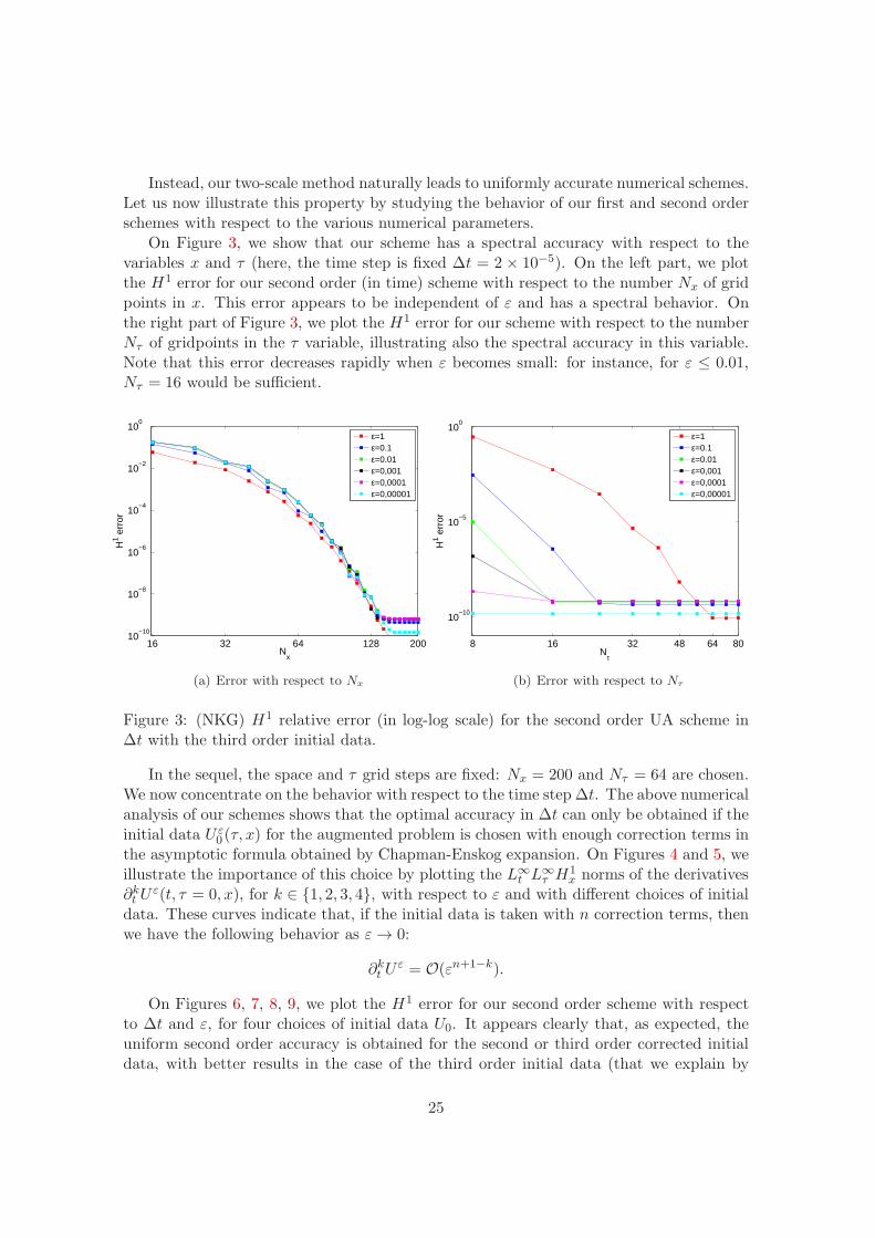
On Figure 3, we show that our scheme has a spectral accuracy with respect to thevariables x and τ (here, the time step is fixed ∆t = 2 × 10−5). On the left part, we plotthe H1 error for our second order (in time) scheme with respect to the number Nx of gridpoints in x. This error appears to be independent of ε and has a spectral behavior. Onthe right part of Figure 3, we plot the H1 error for our scheme with respect to the numberNτ of gridpoints in the τ variable, illustrating also the spectral accuracy in this variable.Note that this error decreases rapidly when ε becomes small: for instance, for ε ≤ 0.01,Nτ = 16 would be sufficient.

16 32 64 128 20010

−10

10−8

10−6

10−4

10−2

100

Nx

H1 e

rror

ε=1ε=0.1ε=0.01ε=0,001ε=0,0001ε=0,00001

(a) Error with respect to Nx

8 16 32 48 64 80

10−10

10−5

100

Nτ

H1 e

rror

ε=1ε=0.1ε=0.01ε=0,001ε=0,0001ε=0,00001

(b) Error with respect to Nτ

Figure 3: (NKG) H1 relative error (in log-log scale) for the second order UA scheme in∆t with the third order initial data.

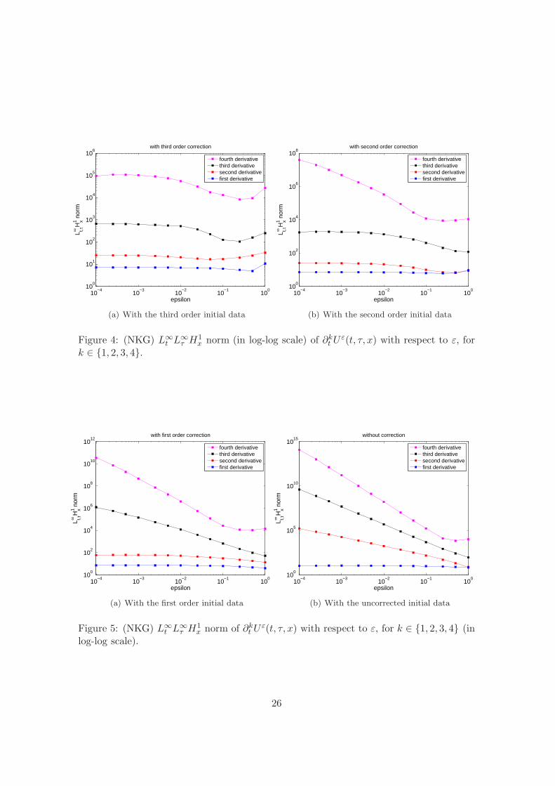
In the sequel, the space and τ grid steps are fixed: Nx = 200 and Nτ = 64 are chosen.We now concentrate on the behavior with respect to the time step ∆t. The above numericalanalysis of our schemes shows that the optimal accuracy in ∆t can only be obtained if theinitial data U ε

0 (τ, x) for the augmented problem is chosen with enough correction terms inthe asymptotic formula obtained by Chapman-Enskog expansion. On Figures 4 and 5, weillustrate the importance of this choice by plotting the L∞

t L∞τ H

1x norms of the derivatives

∂kt Uε(t, τ = 0, x), for k ∈ {1, 2, 3, 4}, with respect to ε and with different choices of initial

data. These curves indicate that, if the initial data is taken with n correction terms, thenwe have the following behavior as ε→ 0:

∂kt Uε = O(εn+1−k).

On Figures 6, 7, 8, 9, we plot the H1 error for our second order scheme with respectto ∆t and ε, for four choices of initial data U0. It appears clearly that, as expected, theuniform second order accuracy is obtained for the second or third order corrected initialdata, with better results in the case of the third order initial data (that we explain by

25

10−4

10−3

10−2

10−1

100

100

101

102

103

104

105

106

epsilon

L∞ t,τH

1 x nor

m

with third order correction

fourth derivativethird derivativesecond derivativefirst derivative

(a) With the third order initial data

10−4

10−3

10−2

10−1

100

100

102

104

106

108

epsilon

L∞ t,τH

1 x nor

m

with second order correction

fourth derivativethird derivativesecond derivativefirst derivative

(b) With the second order initial data

Figure 4: (NKG) L∞t L

∞τ H

1x norm (in log-log scale) of ∂kt U

ε(t, τ, x) with respect to ε, fork ∈ {1, 2, 3, 4}.

10−4

10−3

10−2

10−1

100

100

102

104

106

108

1010

1012

epsilon

L∞ t,τH

1 x nor

m

with first order correction

fourth derivativethird derivativesecond derivativefirst derivative

(a) With the first order initial data

10−4

10−3

10−2

10−1

100

100

105

1010

1015

epsilon

L∞ t,τH

1 x nor

m

without correction

fourth derivativethird derivativesecond derivativefirst derivative

(b) With the uncorrected initial data

Figure 5: (NKG) L∞t L

∞τ H

1x norm of ∂kt U

ε(t, τ, x) with respect to ε, for k ∈ {1, 2, 3, 4} (inlog-log scale).

26

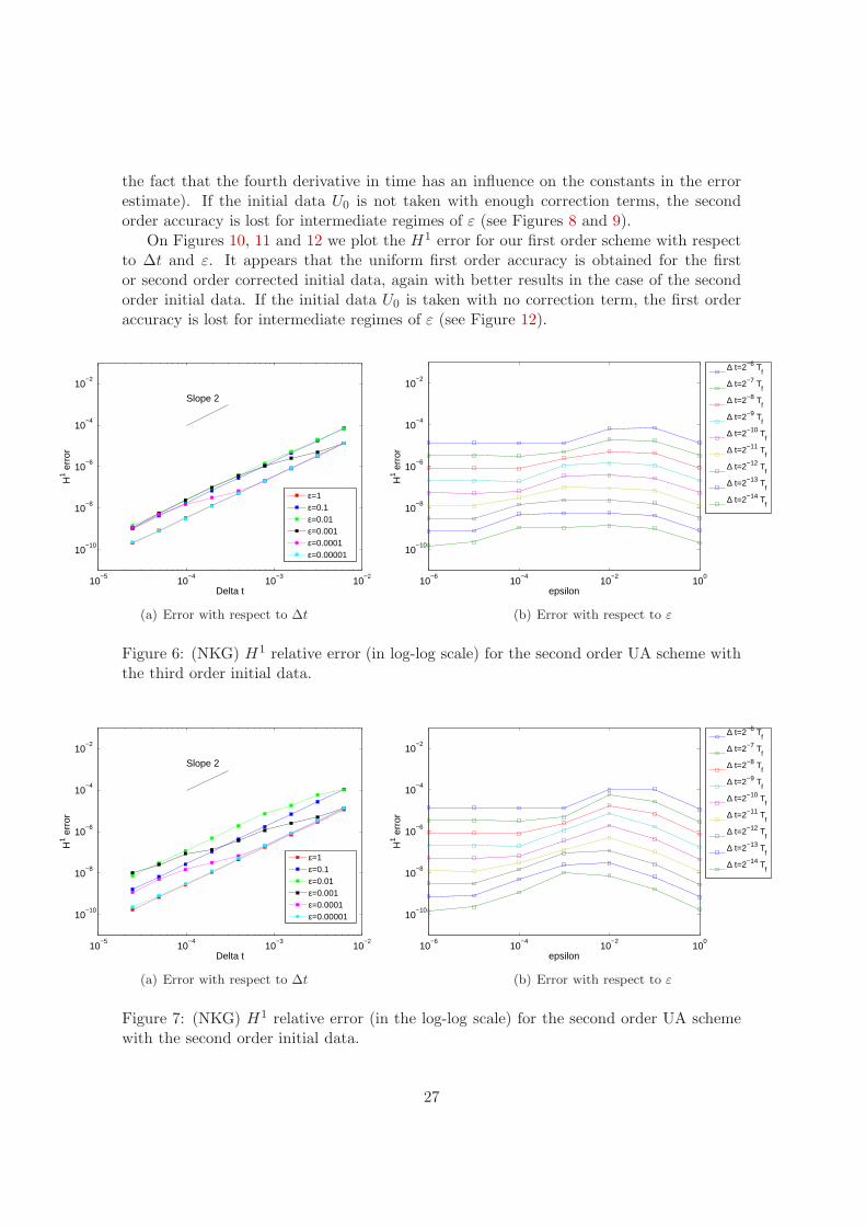
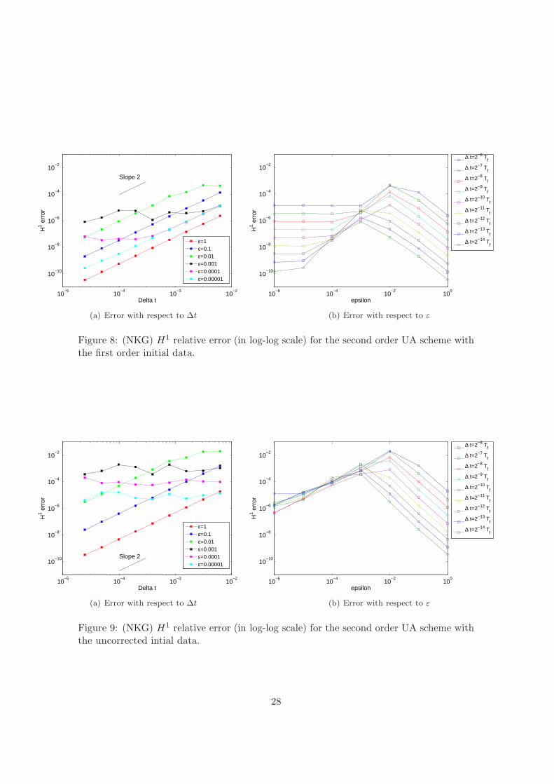
the fact that the fourth derivative in time has an influence on the constants in the errorestimate). If the initial data U0 is not taken with enough correction terms, the secondorder accuracy is lost for intermediate regimes of ε (see Figures 8 and 9).

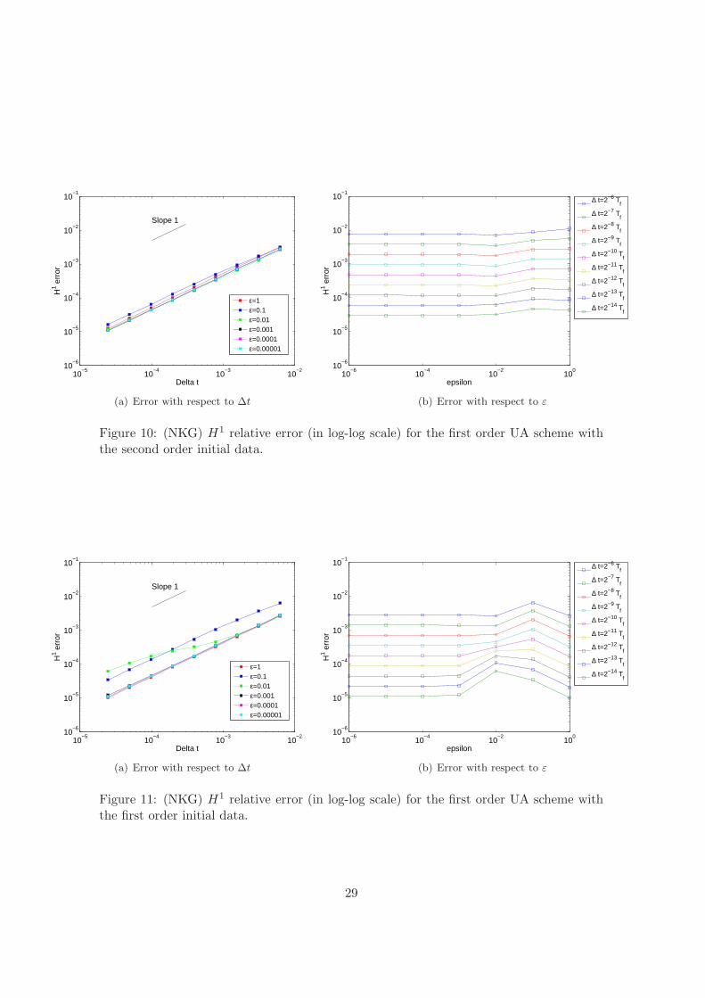
On Figures 10, 11 and 12 we plot the H1 error for our first order scheme with respectto ∆t and ε. It appears that the uniform first order accuracy is obtained for the firstor second order corrected initial data, again with better results in the case of the secondorder initial data. If the initial data U0 is taken with no correction term, the first orderaccuracy is lost for intermediate regimes of ε (see Figure 12).

10−5

10−4

10−3

10−2

10−10

10−8

10−6

10−4

10−2

Delta t

H1 e

rror

Slope 2

ε=1ε=0.1ε=0.01ε=0.001ε=0.0001ε=0.00001

(a) Error with respect to ∆t

10−6

10−4

10−2

100

10−10

10−8

10−6

10−4

10−2

epsilon

H1 e

rror

∆ t=2−6 Tf

∆ t=2−7 Tf

∆ t=2−8 Tf

∆ t=2−9 Tf

∆ t=2−10 Tf

∆ t=2−11 Tf

∆ t=2−12 Tf

∆ t=2−13 Tf

∆ t=2−14 Tf

(b) Error with respect to ε

Figure 6: (NKG) H1 relative error (in log-log scale) for the second order UA scheme withthe third order initial data.

10−5

10−4

10−3

10−2

10−10

10−8

10−6

10−4

10−2

Delta t

H1 e

rror

Slope 2

ε=1ε=0.1ε=0.01ε=0.001ε=0.0001ε=0.00001

(a) Error with respect to ∆t

10−6

10−4

10−2

100

10−10

10−8

10−6

10−4

10−2

epsilon

H1 e

rror

∆ t=2−6 Tf

∆ t=2−7 Tf

∆ t=2−8 Tf

∆ t=2−9 Tf

∆ t=2−10 Tf

∆ t=2−11 Tf

∆ t=2−12 Tf

∆ t=2−13 Tf

∆ t=2−14 Tf

(b) Error with respect to ε

Figure 7: (NKG) H1 relative error (in the log-log scale) for the second order UA schemewith the second order initial data.

27

10−5

10−4

10−3

10−2

10−10

10−8

10−6

10−4

10−2

Delta t

H1 e

rror

Slope 2

ε=1ε=0.1ε=0.01ε=0.001ε=0.0001ε=0.00001

(a) Error with respect to ∆t

10−6

10−4

10−2

100

10−10

10−8

10−6

10−4

10−2

epsilon

H1 e

rror

∆ t=2−6 Tf

∆ t=2−7 Tf

∆ t=2−8 Tf

∆ t=2−9 Tf

∆ t=2−10 Tf

∆ t=2−11 Tf

∆ t=2−12 Tf

∆ t=2−13 Tf

∆ t=2−14 Tf

(b) Error with respect to ε

Figure 8: (NKG) H1 relative error (in log-log scale) for the second order UA scheme withthe first order initial data.

10−5

10−4

10−3

10−2

10−10

10−8

10−6

10−4

10−2

Delta t

H1 e

rror

Slope 2

ε=1ε=0.1ε=0.01ε=0.001ε=0.0001ε=0.00001

(a) Error with respect to ∆t

10−6

10−4

10−2

100

10−10

10−8

10−6

10−4

10−2

epsilon

H1 e

rror

∆ t=2−6 Tf

∆ t=2−7 Tf

∆ t=2−8 Tf

∆ t=2−9 Tf

∆ t=2−10 Tf

∆ t=2−11 Tf

∆ t=2−12 Tf

∆ t=2−13 Tf

∆ t=2−14 Tf

(b) Error with respect to ε

Figure 9: (NKG) H1 relative error (in log-log scale) for the second order UA scheme withthe uncorrected intial data.

28

10−5

10−4

10−3

10−2

10−6

10−5

10−4

10−3

10−2

10−1

Delta t

H1 e

rror

Slope 1

ε=1ε=0.1ε=0.01ε=0.001ε=0.0001ε=0.00001

(a) Error with respect to ∆t

10−6

10−4

10−2

100

10−6

10−5

10−4

10−3

10−2

10−1

epsilon

H1 e

rror

∆ t=2−6 Tf

∆ t=2−7 Tf

∆ t=2−8 Tf

∆ t=2−9 Tf

∆ t=2−10 Tf

∆ t=2−11 Tf

∆ t=2−12 Tf

∆ t=2−13 Tf

∆ t=2−14 Tf

(b) Error with respect to ε

Figure 10: (NKG) H1 relative error (in log-log scale) for the first order UA scheme withthe second order initial data.

10−5

10−4

10−3

10−2

10−6

10−5

10−4

10−3

10−2

10−1

Delta t

H1 e

rror

Slope 1

ε=1ε=0.1ε=0.01ε=0.001ε=0.0001ε=0.00001

(a) Error with respect to ∆t

10−6

10−4

10−2

100

10−6

10−5

10−4

10−3

10−2

10−1

epsilon

H1 e

rror

∆ t=2−6 Tf

∆ t=2−7 Tf

∆ t=2−8 Tf

∆ t=2−9 Tf

∆ t=2−10 Tf

∆ t=2−11 Tf

∆ t=2−12 Tf

∆ t=2−13 Tf

∆ t=2−14 Tf

(b) Error with respect to ε

Figure 11: (NKG) H1 relative error (in log-log scale) for the first order UA scheme withthe first order initial data.

29

10−5

10−4

10−3

10−2

10−6

10−5

10−4

10−3

10−2

10−1

Delta t

H1 e

rror

Slope 1

ε=1ε=0.1ε=0.01ε=0.001ε=0.0001ε=0.00001

(a) Error with respect to ∆t

10−6

10−4

10−2

100

10−6

10−5

10−4

10−3

10−2

10−1

epsilon

H1 e

rror

∆ t=2−6 Tf

∆ t=2−7 Tf

∆ t=2−8 Tf

∆ t=2−9 Tf

∆ t=2−10 Tf

∆ t=2−11 Tf

∆ t=2−12 Tf

∆ t=2−13 Tf

∆ t=2−14 Tf

(b) Error with respect to ε

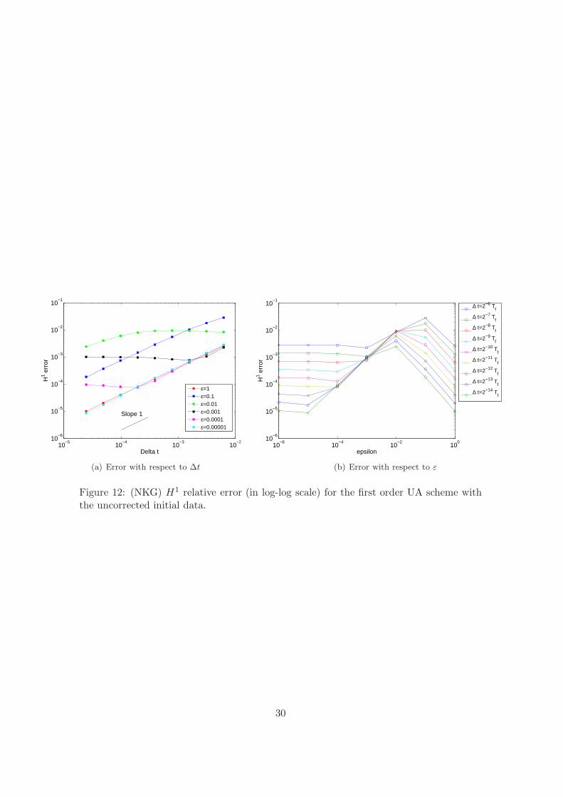
Figure 12: (NKG) H1 relative error (in log-log scale) for the first order UA scheme withthe uncorrected initial data.

30

5.2 The nonlinear Schrodinger equation in a highly oscillatory regime

In this subsection, we consider the cubic nonlinear Schrodinger (NLS) equation under thefollowing form:

i∂tu = −1

ε∆u+ γ(x)|u|2u, u(0, x) = u0(x), (5.11)

on the torus x ∈ [0, a]d.For numerical simulations, our precise example is the one in dimension d = 1 studied

in [9] and in [3]. We take γ(x) = 2 cos(2x), the space domain in x is [0, 2π], the initialdata is

u0(x) = cos x+ sinx

and the final time of the simulation is Tf = 0.4.As for the nonlinear Klein-Gordon case, let us first show that (5.11) fits with our

general framework. The filtered wavefunction

u = e−i tε∆u,

satisfies the equation

i∂tu = e−i tε∆

(γ(x)

∣∣∣eitε∆u

∣∣∣2ei

tε∆u

),

which is again under the form (2.1) with

F(t, τ, u, ε) = −ie−iτ∆(γ∣∣eiτ∆u

∣∣2 eiτ∆u). (5.12)

Here again, it can be checked that this vector field F satisfies Assumption (A). Thespectrum of the Laplace operator −∆ on the torus x ∈ [0, a]d is

{(2π/a)2|k|2 = (2π/a)2 (k21 + · · · + k2d) ; k ∈ Z

d}⊂ (2π/a)2N

so that τ 7→ eiτ∆ is periodic, with period P = a2

2π , and F is also periodic w.r.t. τ .

In order to validate our approach, we now proceed with similar numerical tests asin the case of the NKG equation. The reference solution is computed as follows. Forε ≥ 10−2, we use the Yoshida fourth order splitting method [17] with ∆x = 2π/128,∆t = ε Tf/32768. For smaller values of ε, we rather use our second order scheme, withthe following parameters: ∆x = 2π/128 ≈ 0.05, ∆t = 2π/512000 ≈ 1.2 × 10−5, ∆τ =2π/4096 ≈ 1.5 × 10−3.

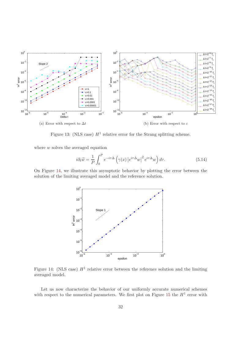
We first plot on Figure 13 the H1 error between the numerical solution computedwith the standard Strang splitting scheme for NLS (with a fixed, large enough, number ofpoints in x, Nx = 128) and the reference solution. It appears again that the error behaves

asymptotically like C∆t2

ε , where C does not depend on ∆t and ε.As ε→ 0, the solution of (5.11) behaves as

‖u(t, x) − eitε∆w(t, x)‖ ≤ Cε, (5.13)

31

10−6

10−5

10−4

10−3

10−2

10−12

10−10

10−8

10−6

10−4

10−2

100

Delta t

H1 e

rror

Slope 2

ε=1ε=0.1ε=0.01ε=0.001ε=0.0001ε=0.00001

(a) Error with respect to ∆t

10−6

10−4

10−2

100

10−12

10−10

10−8

10−6

10−4

10−2

100

epsilon

H1 e

rror

∆ t=2−6 Tf

∆ t=2−7 Tf

∆ t=2−8 Tf

∆ t=2−9 Tf

∆ t=2−10 Tf

∆ t=2−11 Tf

∆ t=2−12 Tf

∆ t=2−13 Tf

∆ t=2−14 Tf

∆ t=2−15 Tf

∆ t=2−16 Tf

∆ t=2−17 Tf

∆ t=2−18 Tf

(b) Error with respect to ε

Figure 13: (NLS case) H1 relative error for the Strang splitting scheme.

where w solves the averaged equation

i∂tw =1

P

∫ P

0e−iτ∆

(γ(x)

∣∣eiτ∆w∣∣2 eiτ∆w

)dτ. (5.14)

On Figure 14, we illustrate this asymptotic behavior by plotting the error between thesolution of the limiting averaged model and the reference solution.

10−6

10−4

10−2

100

10−6

10−5

10−4

10−3

10−2

10−1

100

epsilon

H1 e

rror

Slope 1

Figure 14: (NLS case) H1 relative error between the reference solution and the limitingaveraged model.

Let us now characterize the behavior of our uniformly accurate numerical schemeswith respect to the numerical parameters. We first plot on Figure 15 the H1 error with

32

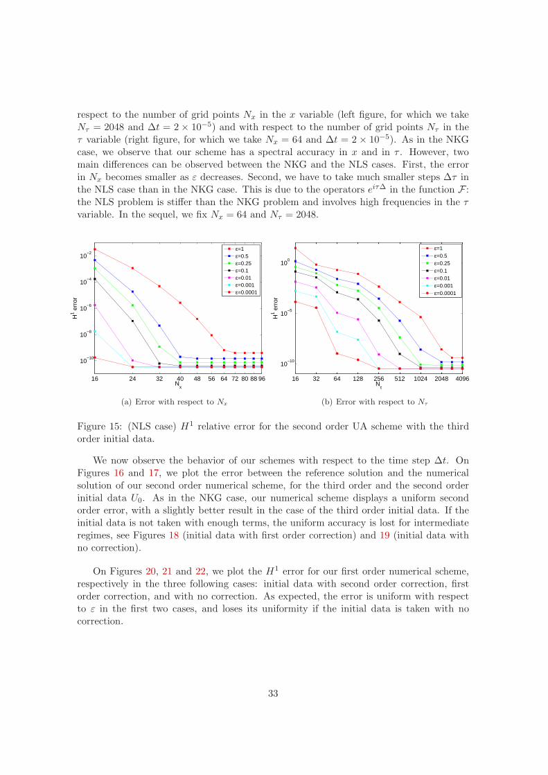
respect to the number of grid points Nx in the x variable (left figure, for which we takeNτ = 2048 and ∆t = 2× 10−5) and with respect to the number of grid points Nτ in theτ variable (right figure, for which we take Nx = 64 and ∆t = 2 × 10−5). As in the NKGcase, we observe that our scheme has a spectral accuracy in x and in τ . However, twomain differences can be observed between the NKG and the NLS cases. First, the errorin Nx becomes smaller as ε decreases. Second, we have to take much smaller steps ∆τ inthe NLS case than in the NKG case. This is due to the operators eiτ∆ in the function F :the NLS problem is stiffer than the NKG problem and involves high frequencies in the τvariable. In the sequel, we fix Nx = 64 and Nτ = 2048.

16 24 32 40 48 56 64 72 80 88 96

10−10

10−8

10−6

10−4

10−2

Nx

H1 e

rror

ε=1ε=0.5ε=0.25ε=0.1ε=0.01ε=0.001ε=0.0001

(a) Error with respect to Nx

16 32 64 128 256 512 1024 2048 4096

10−10

10−5

100

Nτ

H1 e

rror

ε=1ε=0.5ε=0.25ε=0.1ε=0.01ε=0.001ε=0.0001

(b) Error with respect to Nτ

Figure 15: (NLS case) H1 relative error for the second order UA scheme with the thirdorder initial data.

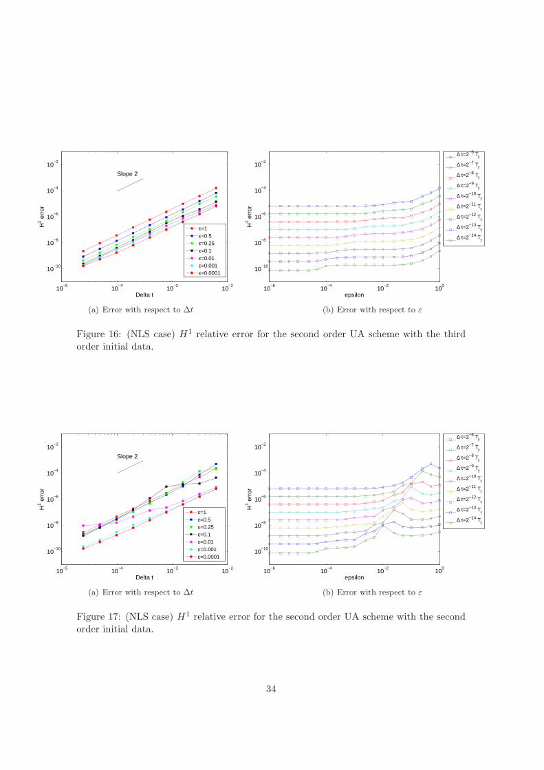
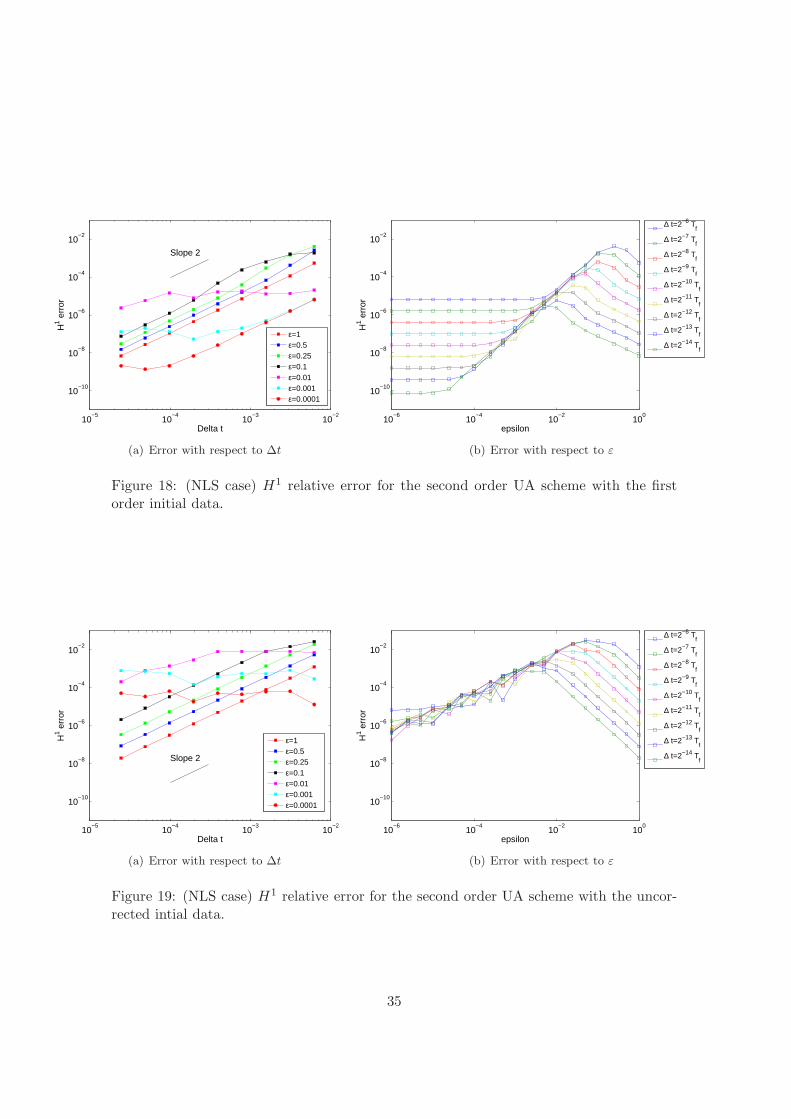
We now observe the behavior of our schemes with respect to the time step ∆t. OnFigures 16 and 17, we plot the error between the reference solution and the numericalsolution of our second order numerical scheme, for the third order and the second orderinitial data U0. As in the NKG case, our numerical scheme displays a uniform secondorder error, with a slightly better result in the case of the third order initial data. If theinitial data is not taken with enough terms, the uniform accuracy is lost for intermediateregimes, see Figures 18 (initial data with first order correction) and 19 (initial data withno correction).

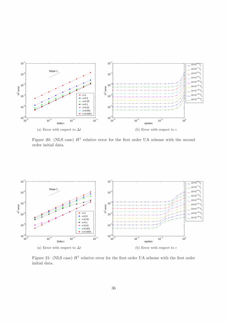
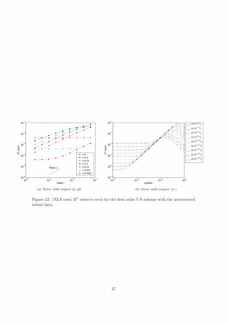
On Figures 20, 21 and 22, we plot the H1 error for our first order numerical scheme,respectively in the three following cases: initial data with second order correction, firstorder correction, and with no correction. As expected, the error is uniform with respectto ε in the first two cases, and loses its uniformity if the initial data is taken with nocorrection.

33

10−5

10−4

10−3

10−2

10−10

10−8

10−6

10−4

10−2

Delta t

H1 e

rror

Slope 2

ε=1ε=0.5ε=0.25ε=0.1ε=0.01ε=0.001ε=0.0001

(a) Error with respect to ∆t

10−6

10−4

10−2

100

10−10

10−8

10−6

10−4

10−2

epsilon

H1 e

rror

∆ t=2−6 Tf

∆ t=2−7 Tf

∆ t=2−8 Tf

∆ t=2−9 Tf

∆ t=2−10 Tf

∆ t=2−11 Tf

∆ t=2−12 Tf

∆ t=2−13 Tf

∆ t=2−14 Tf

(b) Error with respect to ε

Figure 16: (NLS case) H1 relative error for the second order UA scheme with the thirdorder initial data.

10−5

10−4

10−3

10−2

10−10

10−8

10−6

10−4

10−2

Delta t

H1 e

rror

Slope 2

ε=1ε=0.5ε=0.25ε=0.1ε=0.01ε=0.001ε=0.0001

(a) Error with respect to ∆t

10−6

10−4

10−2

100

10−10

10−8

10−6

10−4

10−2

epsilon

H1 e

rror

∆ t=2−6 Tf

∆ t=2−7 Tf

∆ t=2−8 Tf

∆ t=2−9 Tf

∆ t=2−10 Tf

∆ t=2−11 Tf

∆ t=2−12 Tf

∆ t=2−13 Tf

∆ t=2−14 Tf

(b) Error with respect to ε

Figure 17: (NLS case) H1 relative error for the second order UA scheme with the secondorder initial data.

34

10−5

10−4

10−3

10−2

10−10

10−8

10−6

10−4

10−2

Delta t

H1 e

rror

Slope 2

ε=1ε=0.5ε=0.25ε=0.1ε=0.01ε=0.001ε=0.0001

(a) Error with respect to ∆t

10−6

10−4

10−2

100

10−10

10−8

10−6

10−4

10−2

epsilon

H1 e

rror

∆ t=2−6 Tf

∆ t=2−7 Tf

∆ t=2−8 Tf

∆ t=2−9 Tf

∆ t=2−10 Tf

∆ t=2−11 Tf

∆ t=2−12 Tf

∆ t=2−13 Tf

∆ t=2−14 Tf

(b) Error with respect to ε

Figure 18: (NLS case) H1 relative error for the second order UA scheme with the firstorder initial data.

10−5

10−4

10−3

10−2

10−10

10−8

10−6

10−4

10−2

Delta t

H1 e

rror

Slope 2

ε=1ε=0.5ε=0.25ε=0.1ε=0.01ε=0.001ε=0.0001

(a) Error with respect to ∆t

10−6

10−4

10−2

100

10−10

10−8

10−6

10−4

10−2

epsilon

H1 e

rror

∆ t=2−6 Tf

∆ t=2−7 Tf

∆ t=2−8 Tf

∆ t=2−9 Tf

∆ t=2−10 Tf

∆ t=2−11 Tf

∆ t=2−12 Tf

∆ t=2−13 Tf

∆ t=2−14 Tf

(b) Error with respect to ε

Figure 19: (NLS case) H1 relative error for the second order UA scheme with the uncor-rected intial data.

35

10−5

10−4

10−3

10−2

10−6

10−5

10−4

10−3

10−2

10−1

Delta t

H1 e

rror

Slope 1

ε=1ε=0.5ε=0.25ε=0.1ε=0.01ε=0.001ε=0.0001

(a) Error with respect to ∆t

10−6

10−4

10−2

100

10−6

10−5

10−4

10−3

10−2

10−1

epsilon

H1 e

rror

∆ t=2−6 Tf

∆ t=2−7 Tf

∆ t=2−8 Tf

∆ t=2−9 Tf

∆ t=2−10 Tf

∆ t=2−11 Tf

∆ t=2−12 Tf

∆ t=2−13 Tf

∆ t=2−14 Tf

(b) Error with respect to ε

Figure 20: (NLS case) H1 relative error for the first order UA scheme with the secondorder initial data.

10−5

10−4

10−3

10−2

10−6

10−5

10−4

10−3

10−2

10−1

Delta t

H1 e

rror

Slope 1

ε=1ε=0.5ε=0.25ε=0.1ε=0.01ε=0.001ε=0.0001

(a) Error with respect to ∆t

10−6

10−4

10−2

100

10−6

10−5

10−4

10−3

10−2

10−1

epsilon

H1 e

rror

∆ t=2−6 Tf

∆ t=2−7 Tf

∆ t=2−8 Tf

∆ t=2−9 Tf

∆ t=2−10 Tf

∆ t=2−11 Tf

∆ t=2−12 Tf

∆ t=2−13 Tf

∆ t=2−14 Tf

(b) Error with respect to ε

Figure 21: (NLS case) H1 relative error for the first order UA scheme with the first orderinitial data.

36

10−5

10−4

10−3

10−2

10−6

10−5

10−4

10−3

10−2

10−1

Delta t

H1 e

rror

Slope 1

ε=1ε=0.5ε=0.25ε=0.1ε=0.01ε=0.001ε=0.0001

(a) Error with respect to ∆t

10−6

10−4

10−2

100

10−6

10−5

10−4

10−3

10−2

10−1

epsilon

H1 e

rror

∆ t=2−6 Tf

∆ t=2−7 Tf

∆ t=2−8 Tf

∆ t=2−9 Tf

∆ t=2−10 Tf

∆ t=2−11 Tf

∆ t=2−12 Tf

∆ t=2−13 Tf

∆ t=2−14 Tf

(b) Error with respect to ε

Figure 22: (NLS case) H1 relative error for the first order UA scheme with the uncorrectedinitial data.

37

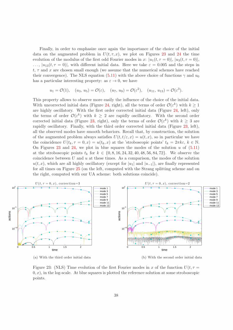
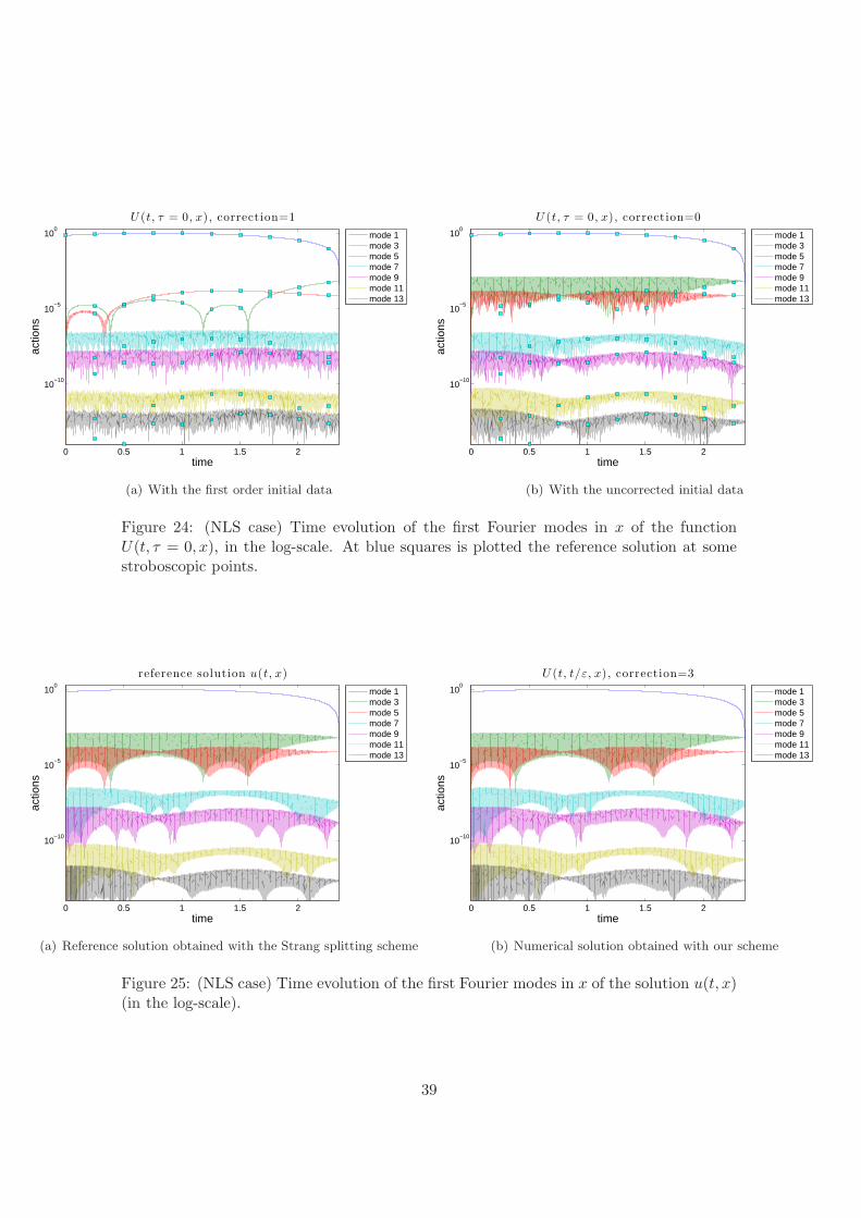
Finally, in order to emphasize once again the importance of the choice of the initialdata on the augmented problem in U(t, τ, x), we plot on Figures 23 and 24 the timeevolution of the modulus of the first odd Fourier modes in x: |u1(t, τ = 0)|, |u3(t, τ = 0)|,. . . , |u13(t, τ = 0)|, with different initial data. Here we take ε = 0.005 and the steps int, τ and x are chosen small enough (we assume that the numerical schemes have reachedtheir convergence). The NLS equation (5.11) with the above choice of functions γ and u0has a particular interesting property: as ε→ 0, we have

u1 = O(1), (u3, u5) = O(ε), (u7, u9) = O(ε2), (u11, u13) = O(ε3).

This property allows to observe more easily the influence of the choice of the initial data.With uncorrected initial data (Figure 24, right), all the terms of order O(εk) with k ≥ 1are highly oscillatory. With the first order corrected initial data (Figure 24, left), onlythe terms of order O(εk) with k ≥ 2 are rapidly oscillatory. With the second ordercorrected initial data (Figure 23, right), only the terms of order O(εk) with k ≥ 3 arerapidly oscillatory. Finally, with the third order corrected initial data (Figure 23, left),all the observed modes have smooth behaviors. Recall that, by construction, the solutionof the augmented problem always satisfies U(t, t/ε, x) = u(t, x), so in particular we havethe coincidence U(tk, τ = 0, x) = u(tk, x) at the ’stroboscopic points’ tk = 2πkε, k ∈ N.On Figures 23 and 24, we plot in blue squares the modes of the solution u of (5.11)at the stroboscopic points tk for k ∈ {0, 8, 16, 24, 32, 40, 48, 56, 84, 72}. We observe thecoincidence between U and u at these times. As a comparison, the modes of the solutionu(t, x), which are all highly oscillatory (except for |u1| and |u−1|), are finally representedfor all times on Figure 25 (on the left, computed with the Strang splitting scheme and onthe right, computed with our UA scheme: both solutions coincide).

0 0.5 1 1.5 2

10−10

10−5

100

time

actio

ns

U (t, τ = 0, x), correction=3

mode 1mode 3mode 5mode 7mode 9mode 11mode 13

(a) With the third order initial data

0 0.5 1 1.5 2

10−10

10−5

100

time

actio

ns

U (t, τ = 0, x), correction=2

mode 1mode 3mode 5mode 7mode 9mode 11mode 13

(b) With the second order initial data

Figure 23: (NLS) Time evolution of the first Fourier modes in x of the function U(t, τ =0, x), in the log-scale. At blue squares is plotted the reference solution at some stroboscopicpoints.

38

0 0.5 1 1.5 2

10−10

10−5

100

time

actio

ns

U (t, τ = 0, x), correction=1

mode 1mode 3mode 5mode 7mode 9mode 11mode 13

(a) With the first order initial data

0 0.5 1 1.5 2

10−10

10−5

100

time

actio

ns

U (t, τ = 0, x), correction=0

mode 1mode 3mode 5mode 7mode 9mode 11mode 13

(b) With the uncorrected initial data

Figure 24: (NLS case) Time evolution of the first Fourier modes in x of the functionU(t, τ = 0, x), in the log-scale. At blue squares is plotted the reference solution at somestroboscopic points.

0 0.5 1 1.5 2

10−10

10−5

100

time

actio

ns

reference solution u(t, x)

mode 1mode 3mode 5mode 7mode 9mode 11mode 13

(a) Reference solution obtained with the Strang splitting scheme

0 0.5 1 1.5 2

10−10

10−5

100

time

actio

ns

U (t, t/ε, x), correction=3

mode 1mode 3mode 5mode 7mode 9mode 11mode 13

(b) Numerical solution obtained with our scheme

Figure 25: (NLS case) Time evolution of the first Fourier modes in x of the solution u(t, x)(in the log-scale).

39

References

[1] G. Allaire, Homogenization and two-scale convergence, SIAM J. Math. Anal. 23,1482–1518, 1992.

[2] W. Bao, X. Dong, Analysis and comparison of numerical methods for the Klein-Gordon equation in the nonrelativistic limit regime, Numer. Math. 120, 189–229, 2012.

[3] F. Castella, P. Chartier, A. Murua, F. Mehats, Stroboscopic averagingfor the nonlinear Schrodinger equation, preprint HAL-00732850 (http://hal.archives-ouvertes.fr).

[4] P. Chartier, A. Murua, J. M. Sanz-Serna, Higher-order averaging, formal seriesand numerical integration I: B-series, Found. Comput. Math., 10, No. 6, 695–727,2010.

[5] N. Crouseilles, M. Lemou, F. Mehats, Asymptotic preserving schemes for highlyoscillatory kinetic equations, J. Comp. Phys. 248, 287–308, 2013.

[6] P. Degond, Macroscopic limits of the Boltzmann equation: a review in Modeling andcomputational methods for kinetic equations, P. Degond, L. Pareschi, G. Russo (eds),Modeling and Simulation in Science, Engineering and Technology Series, Birkhauser,2003, pp. 3–57.

[7] E. Faou, K. Schratz, Asymptotic Preserving schemes for the Klein-Gordon equationin the non-relativistic limit regime, to appear in Numer. Math.

[8] E. Frenod, P.-A. Raviart, E. Sonnendrucker, Two scale expansion of a singu-larly perturbed convection equation, J. Maths. Pures Appl. 80, 815–843, 2001.

[9] B. Grebert, C. Villegas-Blas, On the energy exchange between resonant modesin nonlinear Schrodinger equations, Ann. Inst. H. Poincare Anal. Non Lineaire 28,127–134, 2011.

[10] S. Jin, Efficient asymptotic-preserving (AP) schemes for some multiscale kineticequations, SIAM J. Sci. Comput. 21, 441–454, 1999.

[11] S. Machihara, The nonrelativistic limit of the nonlinear Klein-Gordon equation,Funkcial. Ekvac. 44, 243–252, 2001.

[12] S. Machihara, K. Nakanishi, T. Ozawa, Nonrelativistic limit in the energy spacefor nonlinear Klein- Gordon equations, Math. Ann. 322, 603–621, 2002.

[13] N. Masmoudi, K. Nakanishi, From nonlinear Klein-Gordon equation to a systemof coupled nonlinear Schrodinger equations, Math. Ann. 324, 359–389, 2002.

[14] G. Nguetseng, A general convergence result for a functional related to the theoryof homogenization, SIAM J. Math. Anal. 20, 608–623, 1989.

[15] L. M. Perko, Higher order averaging and related methods for perturbed periodic andquasi-periodic systems, SIAM J. Applied. Math. 17, 698–724, 1969.

40

[16] J. A. Sanders, F. Verhulst, Averaging methods in nonlinear dynamical systems,Applied Mathematical Sciences, Vol. 59. Springer-Verlag, 1985.

[17] H. Yoshida, Construction of higher order symplectic integrators, Phys. Lett. A 150no. 5-7, 262–268, 1990.

41