Phenomenological model of bacterial aerotaxis with a

Nonlinear Analysis: Modelling and Control, 2013, Vol. 18, No. 2, 227–249 227

Phenomenological model of bacterial aerotaxiswith a negative feedback∗

Vladas Skakauskasa,1, Pranas Katauskisa, Remigijus Šimkusb,Feliksas Ivanauskasa

aFaculty of Mathematics and Informatics, Vilnius UniversityLT-03225 Vilnius, [email protected]; [email protected]; [email protected] University Institute of BiochemistryLT-08662 Vilnius, [email protected]

Received: 25 June 2012 / Revised: 26 February 2013 / Published online: 18 April 2013

Abstract. A phenomenological model for the suspension of the aerotactic swimming micro-organisms placed in a chamber with its upper surface open to air is presented. The model wasconstructed to embody some complexity of the aerotaxis phenomenon, especially, changes inthe average bacteria drift velocity under changing environmental conditions. It was assumed thateffective forces applied to the cell (gravitational, drag, and thrust) should be essential for theoverall system dynamics; and that bacterial propulsion force, but not their swimming velocity, isproportional to the gradient of the oxygen concentration. Mathematically, the model consists ofthree coupled equations for the oxygen dynamics; for the cell conservation; and for the balance offorces acting on bacteria. An analytical steady-state solution is given for the shallow and deep layersand numerical results are given for the steady-state and initial value problems which are comparedwith corresponding ones to the Keller–Segel model.

Keywords: bioconvection, thermo-bioconvection, swimming microorganisms, oxytactic bacteria.

1 Introduction

The term aerotaxis (or oxytaxis) refers to the situation where bacterium moves towardsor away from air or oxygen. Aerotaxis can be regarded as a kind of the more generalprocess, chemotaxis, which is a motion of bacteria towards a favorable chemical field. Thebasic mathematical model in chemotaxis was introduced by Keller and Segel (KS) [1, 2].In its original form this model consists of four coupled reaction–advection–diffusionequations. Under the quasi-steady-state assumptions this model can be reduced to twocoupled parabolic equations for the concentration of microorganisms and the attracting

∗This work was supported by the Research Council of Lithuania (project No. MIP-052/2012).1Corresponding author.

c© Vilnius University, 2013

228 V. Skakauskas et al.

species (attractants). Mathematical modeling of chemotaxis on the basis of the KS modelhas developed into a large and diverse discipline [3, 4]. KS type equations were used todescribe the oxytactic motion of bacteria in a water column as well [5–7]. Hillesdon,Pedley and Kessler (HPK) [6] and Hillesdon and Pedley (HP) [7] considered dynamicsof an oxytactic bacteria Bacillus subtilis suspension placed in a chamber with its uppersurface open to air. In the HPK model the phenomena of gravitational sedimentation,bulk fluid motion, and diffusion of inactive cells were assumed to be negligible. Theassumption that the sedimentation rate is much smaller than the typical cell swimmingspeed is inaccurate in the case of inactive cells [7]. The typical form of the KS model forthe oxytactic bacteria is [5–7]:

∂C

∂t= div(κ1∇C)− κ2(C)B,

∂B

∂t= div

(−κ3(C)B∇C + κ4(C)∇B

).

(1)

Here C and B are the oxygen and cells concentrations, κ1 and κ4(C) are the diffusivityof oxygen and bacterial cells, κ2(C) is the oxygen consumption rate by cells, v =κ3(C)∇C is the oxytactic bacteria drift velocity, κ3(C) is the oxytactic sensitivity, ∇and div are the gradient and divergence operators. In the steady-state, wide chamber, andconstant κ1, . . . , κ4 case, HPK gave an analytic solution of the model for both shallowand deep chambers. In the deep chamber case, the authors neglected diffusion of inactivecells and therefore one constant was not determined. This constant was obtained bynumerically solving the initial value problem. In the time-dependent one-dimensionalcase with constant κ1 and depending on C coefficients κ2, κ3, and κ4, HPK solvedmodel (1) numerically using the method of lines. HP examined the stability of the steady-state solution.

To describe the convective chemotaxis Dombrowski et al. [8], Tuval et al. [9] general-ized the KS model by including the bulk fluid motion. This model describes the collectivebehavior (bioconvection) of a suspension of oxytactic bacteria in an incompressible fluidunder assumptions [10] that the contribution of bacteria to the bacteria–fluid suspensionis sufficiently small and that more detailed cell–cell interactions (e.g., of hydrodynamictype) are neglected. In [10], this model was studied numerically in detail. The solvabilityof the model was examined by Lorz [11], Duan et al. [12], and Di Francesco et al. [13].Becker et al. [14] and Kuznetsov [15, 16] generalized the KS model and studied thebioconvection of oxytactic cells in a fluid saturated porous medium. Kuznetsov also in-vestigated models for the thermo-bioconvection of oxytactic cells in a fluid layer [17–19]and in a fluid saturated porous layer [15, 16] and carried out the stability analysis oftheir steady-state solutions. In all models of bioconvection and thermo-bioconvection,the oxytactic bacteria drift velocity, as in the KS model, is proportional to the gradientof oxygen concentration while the gravitational force is approximated by the buoyancyterm. Papers of Alloui et al. [20,21] are devoted to numerical study of the development ofgravitactic bioconvection and thermo-bioconvection of swimming microorganisms whichare little denser than water and move randomly, but on the average, upwardly against

www.mii.lt/NA

Phenomenological model of bacterial aerotaxis with a negative feedback 229

gravity. Alloui et al. [22] also carried out the linear stability analysis of the thermo-bioconvection of swimming against gravity microorganisms.

We note three problems that arise in mathematical modeling of bacterial aerotaxis.Firstly, it should be noted, that an important aspect of KS chemotaxis models is theexpected onset of chemotactic collapse [3, 4, 23]. This term refers to the fact that, undersuitable circumstances, the whole population should concentrate in a single point in finitetime. However, it seems likely, that real bacterium is searching for the optimal place to be.Therefore, the overcrowding of bacteria in small space domains is unrealistic due to lackof nutrition for population in this domain. A number of modifications have been madeto the minimal KS model of auto-aggregation that allows preventing such unrealisticsingularities [4]. In general, this means, that in real systems there are certain dispersalmechanisms, which can be regarded as a negative chemotaxis and/or the suppression ofthe positive chemotaxis. The corresponding dispersal mechanisms were not taken intoaccount in the KS type models of aerotaxis. Secondly, in real systems, the responseof microorganisms to oxygen is much more complicated than the simplest KS modelsuggests [24–27]. It is known, that dependently on the type of bacteria and local environ-mental conditions, oxygen can act as an attractant or as a repellent ( [24,25] and referencestherein). The positive aerotaxis (oxygen is attractant) results in aggregation of cells at theoxygen-exposed surfaces and the negative aerotaxis (oxygen is repellent) imply dispersalof the cell. Thus, again, a certain mechanism of the suppression of the positive aerotaxisshould be included to the overall dynamic system. Thirdly, a common feature of manychemotaxis models based on the approximation of the cells drift velocity by the gradientof the chemoattractant or chemorepellent is to incorporate some complexity of the chemo-taxis into the equations through a chemotactic sensitivity function (see system (1)). Butdifferent microorganisms detect spatial gradients of the chemical signal through distinctmechanisms. Certain cells [28], such as Dystyostelium discoideum, fibroblasts and leuko-cytes, can detect and respond to a small gradient in the chemical signal across the lengthof their body using a process of internal amplification and polarisation. Smaller cells [29],such as E. coli, detect a gradient by sampling the concentration at different time pointsand modifying their movement accordingly. The observation that the gradient sensedby bacteria is temporal means that bacteria possess a memory, which compares pastinformation with present information to make a decision. This memory is long enoughso that the bacteria can make an accurate comparison between two points more distal thanthe bacterial body length. In both cases, the signal detected by the cell is intrinsicallynon-local and it may therefore be appropriate to consider movement based on non-localgradient by the integration of the signal by the cell over some region. For cells whichdetect a gradient in the chemical signal across the length of their body, Othmer and Hillen[30] approximated their drift velocity by the formula χCn/(ωρ)

∫Sn−1 σB(t, x+ ρσ) dσ

where ω = |Sn−1|, Sn−1 denotes the (n − 1)-dimensional unit sphere in Rn, andρ is the radius of a sphere which enclose the cell. Analytical and numerical study ofthis model is given in [31]. Studies of smaller cells revealed (see [28] and literaturetherein) that, like many other sensory systems, the chemotactic response involves twoprocesses: excitation and adaptation. When bacteria are stimulated, their swimming modeare changed instantaneously. This initial process, termed excitation, is very fast. Later on,

Nonlinear Anal. Model. Control, 2013, Vol. 18, No. 2, 227–249


bacteria resume their prestimulus behaviour, even though the stimulus is still present.This process, termed adaptation, is relatively slow (in the range of seconds or minutes).Adaptation thus enable bacteria to adjust to changes in the stimulus intensity and respondto new stimuli. Models of KS type are based on the quasi-steady-state approximation ofthe cells drift velocity and therefore cannot describe correctly the adaptation period.

The aim of this paper is study of the dynamics of the dilute suspensions of aerotac-tic bacteria by the modified KS model. To describe some complexity of the aerotaxisphenomenon (especially, the bacteria adaptation period under changes in environmentalconditions), we replace the quasi-steady-state equation v = κ3(C)∇C by the momentumequation for cells drift velocity. In the modified model it is assumed that 1) gravitational,drag, and thrust forces applied to the cell are not negligible and 2) that bacterial thrustforce, but not its average drift velocity, is proportional to the gradient of the oxygenconcentration. The model consists of three coupled equations: 1) the equations for oxygendynamics; 2) cell conservation equation; and 3) momentum equation for the cells drift ve-locity. This original model of oxytaxis is termed as FB (Feedback/Force balance) model.In the wide chamber case, we give an analytic solution of the model for both shallowand deep chambers and discuss the numerical results of the initial value and steady-state problems. We also solved the KS model and using numerical results demonstratedifference between the FB and KS models.

The paper is organized as follows. In the auxiliary Section 2, we introduce the KSmodel and give a detail derivation of its steady-state solution found by HPK. In Section 3,we present the FB model and demonstrate its steady-state solution. In Section 4, we com-pare numerical results for the KS and FB models. Some remarks in Section 5 concludethe paper.

2 The one-dimensional Keller–Segel (KS) model

In this auxiliary section, we introduce the KS model and give a detail derivation of itssteady-state solution which was found by HPK [6]. Let x be the vertical coordinate. Inthe one-dimensional case, Eqs. (1) can be written in the form

∂C

∂t=

∂

∂x

(κ1∂C

∂x

)− κ2(C)B, x ∈ (0, h),

∂B

∂t=

∂

∂x

(−κ3(C)B

∂C

∂x+ κ4(C)

∂B

∂x

), x ∈ (0, h),

(2)

C(0, x) = C0, B(0, x) = B0, C(t, h) = C0,

∂C

∂x

∣∣∣∣x=0

=∂B

∂x

∣∣∣∣x=0

= 0,(κ3(C)B

∂C

∂x− κ4(C)

∂B

∂x

)∣∣∣∣x=h

= 0.

(3)

www.mii.lt/NA


Here x = 0 and x = h correspond to the bottom and surface of the chamber, theconstant C0 is the initial and atmosphere oxygen concentration, B0 is the initial cellsconcentration. The total number of cells is equal to the hB0.

Now we introduce the dimensionless variables. Set Θ = (C − Cmin)/(C0 − Cmin),where Cmin is the minimal value of the oxygen concentration necessary for cells tobe active. Let κ2(C) = κ20w2(Θ), κ3(C) = κ30w3(Θ), κ4(C) = κ40w4(Θ), withconstants κ20, κ30, and κ40. Assuming that κ1 is also constant HPK considered the casewhere w2 = w3, w4 = w2

2 , with w2 the Heaviside step function. Set x = hx̄, B = B0B̄,t = (h2/κ40)t̄. Omitting the bar, we rewrite (2), (3) in the dimensionless form

∂Θ

∂t= δ

(∂2Θ

∂x2− β2w2(Θ)B

), x ∈ (0, 1),

∂B

∂t=

∂

∂x

(w4(Θ)

∂B

∂x− αw3(Θ)B

∂Θ

∂x

), x ∈ (0, 1),

∂Θ

∂x

∣∣∣∣x=0

=∂B

∂x

∣∣∣∣x=0

= 0,(w4(Θ)

∂B

∂x− αw3(Θ)B

∂Θ

∂x

)∣∣∣∣x=1

= 0,

Θ(t, 1) = 1,

B(0, x) = Θ(0, x) = 1,

(4)

where δ = κ1/κ40, β2 = B0κ20h2/(κ1(C0 − Cmin)), α = κ30(C0 − Cmin)/κ40.

Note that α is swimming upwards parameter. Integrating over (0, 1) Eq. (4)2 and usingconditions (4)3,4, we get that

∫ 1

0B(t, x) dx = 1 is preserved. In the steady-state case,

system (4) reads

Θ′′ = β2w2(Θ)B,(w4(Θ)B′ − αw3(Θ)BΘ′

)′= 0,

Θ(1) = 1,

w4(1)B′(1)− αw3(1)B(1)Θ′(1) = 0,

Θ′(0) = B′(0) = 0.

(5)

In addition, we formulate the condition1∫

0

B(x) dx = 1. (6)

Now we derive the HPK steady-state solution of system (5) and (6).

2.1 The shallow layer case (Θ > 0 ∀x ∈ (0,1])

Integrating (5)2 and using condition (5)4 we get the equation

w4(Θ)B′ = αw3(Θ)BΘ′. (7)



In this section, we consider the case w2 = w3 = w4 = 1. From (5)1 and (7) we getthe equationB′ = αβ−2θ′θ′′ which has the solutionB = (α/2)β−2(θ′)2+B(0). Hence,

Θ′ = β

√2

α

√B −B(0). (8)

From (7) and (8) we derive the equation

B′ = αβB

√2

α

(B −B(0)

)which has the solution

B = B(0) cos−2(ξx), ξ = β

√αB(0)

2∈(

0,π

2

). (9)

Then combining (8) and (9) we get

Θ′ =2

αξ tan(ξx), Θ(1) = 1.

Hence

Θ = 1− 2

αln

cos(ξx)

cos ξ. (10)

Since Θ must be nonnegative the condition cos(ξx)/ cos ξ 6 eα/2 has to be satisfied forall x ∈ [0, 1]. Hence cos ξ > e−α/2 or cos−2 ξ 6 eα and 0 6 ξ 6 arccos e−α/2. Fromcondition (6) and Eq. (9) we get the equation

q

ξ= tan ξ, (11)

where q = αβ2/2. Eq. (11) has a unique solution ξ = ξ(q) ∈ (0, arccos e−α/2) growingtogether with q since dξ/dq > 0. Then, from Eqs. (9)2 and (11) it follows that B(0) =ξ2(q)/q and cos−2 ξ(q) = 1 + tan2 ξ(q) = 1 + q2/ξ2(q) 6 eα. Thus arccos e−α/2 >ξ(q) > q/

√eα − 1 = αβ2/(2

√eα − 1) and, hence,

β2 6 β2∗ =

2

α

√eα − 1 arccos e−α/2. (12)

Thus θ(0) > 0 if 0 < β < β∗, and θ(0) = 0 if β = β∗. Values of β that satisfy theinequality β 6 β∗ correspond to a shallow chamber. All others correspond to a deepchamber. Note that ∂Θ/∂q = (2/α)(− tan ξ + x tanxξ) dξ/dq < 0 ∀x ∈ (0, 1).

2.2 The deep layer case

In this case β > β∗ and positiveΘ determined by Eq. (10) does not exist for all x ∈ [0, 1].Θ is positive in a layer (x∗, 1],Θ(x∗) = 0, where x∗ > 0 is unknown a priori. There is not

www.mii.lt/NA


enough oxygen available in the layer [0, x∗] and cells are inactive. Therefore w2(Θ) = 0and we have to consider the task Θ′′ = 0, Θ′(0) = Θ(x∗) = 0. Hence, Θ = 0 forall x ∈ [0, x∗]. Independently of w3 and w4 from (7) it follows that B(x) = B(x∗)∀x ∈ [0, x∗], where B(x∗) is also unknown a priori.

HPK neglected diffusion of inactive cells and therefore B(x∗) was not determined bythe conditions of the steady-state case. HPK determined it by solving the initial valueproblem. Differently from HPK, we postulate the continuity of B and B′ at x∗. We alsouse the continuity condition for Θ and Θ′ at x∗. In (x∗, 1] we have to solve Eqs. (5)1,2,3,4and (6). Let w2 = w3 = w4 = 1. By the argument used for the shallow chamber and bythe continuity conditions at x∗ we get

B = B(x∗) cos−2(ξ̃(x− x∗)

), ξ̃ = β

√αB(x∗)

2,

Θ = 1− 2

αln

cos(ξ̃(x− x∗))cos(ξ̃(1− x∗))

> 0(13)

for x ∈ (x∗, 1] and (1− x∗)ξ̃ ∈ (0, π/2). Due to the condition Θ(x∗) = 0 it follows that−α/2 = ln cos(ξ̃(1− x∗)). Hence

tan(ξ̃(1− x∗)

)=√

eα − 1. (14)

At last, from condition (6) we get

1 = B(x∗)x∗ +

1∫x∗

B(x) dx = B(x∗)

(x∗ +

1

ξ̃ tan(ξ̃(1− x∗))

). (15)

Combining the last two equations and using the definition of ξ̃ we get the equation

1 =2ξ̃2

αβ2

(x∗ +

√eα − 1

ξ̃

)which has the solution

ξ̃ =

√eα − 1 + 2x∗αβ2 −

√eα − 1

2x∗. (16)

Now from (14) it follows that (1− x∗)ξ̃ = η(α) := arccos e−α/2. Hence,

1− x∗2x∗

(√eα − 1 + 2x∗αβ2 −

√eα − 1

)= η(α).

This equation has the solution

x∗ = 1− η

√(η −

√eα − 1 )2 + 2αβ2 − (η −

√eα − 1 )

αβ2∈ (0, 1) (17)



such that dx∗/dβ > 0. Combining (16) and (17) we derive an equation for ξ̃ and thenfrom (15) get an equation for B(x∗):

ξ̃ =αβ2√

(η −√

eα − 1 )2 + 2αβ2 − (η −√

eα − 1 )> 0,

B(x∗) =2αβ2

[√

(η −√

eα − 1 )2 + 2αβ2 − (η −√

eα − 1 )]2.

(18)

We see that the steady-state solution does not depend on the positive diffusivity of inactivecells.

In Section 4, we give the numerical solution of the initial value problem (4) deter-mined by using the finite-difference scheme.

3 The feedback/force balance (FB) model

Keller and Segel neglected the bulk fluid velocity and approximated the average ve-locity of swimming upwards oxytactic bacteria by the quasi steady-state formula v =κ3(C)∇C. We also neglect the bulk fluid motion but, to describe some complexity ofthe aerotaxis phenomenon (especially, the bacteria adaptation period under changes inenvironmental conditions), we use the momentum equation for cells which includes thegravitational sedimentation of cells, swimming upwardly strength (force which arisesfrom chemotaxis and enables cells to swim), and resistance force to movement of cellsthrough the fluid. We postulate that swimming upwards strength of cells, but not their av-erage velocity, is parallel and proportional to ∇C. For simplicity, we neglect the bacteriato bacteria communication and convective acceleration, (v ·∇)v, terms in the momentumequation for cells. In the one-dimensional case, the model consists of the equations

∂C

∂t=

∂

∂x

(κ1∂C

∂x

)− κ2(C)B, x ∈ (0, h),

∂B

∂t=

∂

∂x

(−Bv + κ4(C)

∂B

∂x

), x ∈ (0, h),

B∂v

∂t= −Bg̃ − κ5(C)v + κ̃3(C)

∂C

∂x, x ∈ (0, h),

(19)

subject to the conditions

C(0, x) = C0, B(0, x) = B0, v(0, x) = v0,

C(t, h) = C0,∂C

∂x

∣∣∣∣x=0

= 0,(Bv − κ4(C)

∂B

∂x

)∣∣∣∣x=0;h

= 0.

(20)

Here κ1 = const, g̃ = g(1 − ρw/ρB) where g is the acceleration due to the gravity, ρwand ρB are the water (fluid) and a cell density. Note that the dimensions of κ3 in Section 2

www.mii.lt/NA


and κ̃3 in Section 3 are different. Integrating Eq. (19)3 we get a non-local in time equationfor average cells drift velocity v,

v(t, x) = v0(x)Π(0, t, x) +

t∫0

(−B(ξ, x)g̃ + κ̃3

(C(ξ, x)

)∂C(ξ, x)

∂x

)Π(ξ, t, x) dξ

where Π(ξ, t, x) = exp{−∫ tξκ5(C(τ, x)) dτ}.

Let κ2(C) = κ20w2(Θ), κ̃3(C) = κ̃30w3(Θ), κ4(C) = κ40w4(Θ), κ5(C) =κ50w5(Θ), Θ = (C−Cmin)/(C0−Cmin), x = x̄h, B = B0B̄, t = (h2/κ40)t̄, v = v∗v̄.Omitting the bar we rewrite system (19) and (20) in the dimensionless form

∂Θ

∂t= δ

(∂2Θ

∂x2− β2w2(Θ)B

), x ∈ (0, 1),

∂B

∂t=

∂

∂x

(w4(Θ)

∂B

∂x− γBv

), x ∈ (0, 1),

B∂v

∂t= −ρ1B − ρ3w5(Θ)v + ρ2w3(Θ)

∂Θ

∂x, x ∈ (0, 1),

(21)

Θ(0, x) = 1, B(0, x) = 1, v(0, x) = v0,

∂Θ

∂x

∣∣∣∣x=0

= 0, Θ|x=1 = 1,(w4(Θ)

∂B

∂x− γvB

)∣∣∣∣x=0;1

= 0.

(22)

Here δ = κ1/κ40, γ = v∗h/κ40, β2 = B0κ20h2/(κ1(C0−Cmin)), ρ1 = g̃h2/(κ40v∗) =

g̃h3/(γκ240), ρ2 = κ̃30h(C0 − Cmin)/(v∗B0κ40), ρ3 = h2κ50/(B0κ40).Note, that model (21)–(22) preserves condition

∫ 1

0B(t, x) dx = 1. Determining a1 =

ρ1γ/ρ3 and a2 = ρ2γ/ρ3 we rewrite Eq. (21)3 in the form

B∂v

∂t=ρ3γ

(−a1B − γω5(Θ)v + a2ω3(Θ)

∂Θ

∂x

).

Now we consider the steady-state case.

3.1 The shallow chamber case (Θ > 0 ∀x ∈ (0,1])

We study the case where w2(Θ) = w3(Θ) = w4(Θ) = w5(Θ) = 1. From Eqs. (21) and(22) we get

Θ′′ = β2B,

γvB = B′,

v =1

ρ3(ρ2Θ

′ − ρ1B) =a2γΘ′ − a1

γB,

Θ′(0) = 0, Θ(1) = 1.

(23)



In addition, we formulate the condition

1∫0

B(x) dx = 1. (24)

Integrating (23)1 and using (24) we get

Θ′(1) = β2. (25)

Then from Eqs. (23)1,2,3 it follows that

γv =B′

B= β2 dB

dΘ′= a2Θ

′ − a1B. (26)

The last equation of (26) is linear and integrates to get

B(x) = B̂(Θ′, B(0)

)=

(B(0) +

a2a21β2

)exp

(− a1β2Θ′)

+a2a1Θ′ − a2

a21β2. (27)

From (26) we can see that v = 0 and dB/dΘ′ = 0 at B = (ρ2/ρ1)Θ′. Now, insertingthis value of B into (27), we get

Θ′ =β2

a1ln

(1 +

B(0)a21a2β2

). (28)

Then from (26) and (23)1 it follows that

B′′|B=ρ2ρ1Θ′ =

{B′

γ

ρ3(ρ2Θ

′ − ρ1B) +Bγ

ρ3(ρ2Θ

′′ − ρ1B′)}∣∣∣∣

B=(ρ2/ρ1)Θ′

= B2 ρ2ρ3γβ2 > 0.

Hence, (28) is the point of a minimum of B and

minB =ρ2ρ1

β2

a1ln

(1 +

a21B(0)

a2β2

)> 0.

We integrate Eqs. (23)1 and (27) and use condition (23)4 to get

β2x = x̂(Θ′, B(0)

):=

Θ′∫0

dy

B̂(y,B(0)). (29)

From here and by (25) we get the equation for B(0),

β2 =

β2∫0

dy

B̂(y,B(0)). (30)

www.mii.lt/NA


After this equation is solved for B(0), we determine B = B̂(Θ′, B(0)) by Eq. (27),x = x̂(Θ′, B(0)) by Eq. (29), and v by (23)3 for Θ′ ∈ [0, β2].

At last, using (29) we integrate the equation dΘ = Θ′ dx to get

Θ = 1− 1

β2

β2∫Θ′

y dy

B̂(y,B(0)). (31)

This formula shows that Θ > 0 for all x ∈ [0, 1] if

β2 6 β̃2∗ :=

β̃2∗∫

0

y dy

B̂(y,B(0)). (32)

Values β that satisfy condition β 6 β̃∗ correspond to shallow chamber. Substitutingy = β̃2

∗z, B(0) = β̃2∗B̃(0) we rewrite Eqs. (30) and (31) in the form

β̃2∗ =

1∫0

dz

B̃(z, B̃(0)), 1 =

1∫0

z dz

B̃(z, B̃(0)), (33)

where B̃(z, B̃(0)) = (B̃(0) + a2/a21) exp(−a1z) + a2z/a1 − a2/a21.

From (33)2 we determine B̃(0) and then by (33)1 find β̃2∗ . Clearly, β̃2

∗ > 1.

3.2 The deep chamber case (β > β̃∗)

Since function (31) is not positive for all x > 0, we divide (0, 1] into two intervals (0, x̃∗]and (x̃∗, 1], Θ(x̃∗) = 0. In (x̃∗, 1], Θ > 0, and cells consume oxygen and are active.Since Θ(x̃∗) = 0, there is not enough oxygen available in (0, x̃∗). Hence, cells areinactive and therefore κ2(Θ) = 0 ∀x ∈ [0, x̃∗]. Thus in (0, x̃∗) we have the system

Θ′′ = 0, Θ(x̃∗) = 0, Θ′(0) = 0,

γvB = w4(Θ)B′,

v =1

ρ3w5(Θ)

(ρ2ω3(Θ)Θ′ − ρ1B

).

It is easy to see that Θ = 0, v = −ρ1B/(ρ3w5(Θ)) < 0, B′ = −qB2, q = γρ1/(ρ3w4(0)w5(0)) ∀x ∈ (0, x̃∗). Therefore

B(x) =B(x̃∗)

1− qB(x̃∗)(x̃∗ − x)=

B(0)

1 + qxB(0). (34)

In (x̃∗, 1), we consider the case w2 = w3 = w4 = w5 = 1, and solve Eqs. (23) withconditions Θ(1) = 1, Θ(x̃∗) = Θ′(x̃∗) = 0. By the argument used for the shallow



chamber we get

x− x̃∗ =1

β2

Θ′∫0

dy

B̂(y,B(x̃∗)),

Θ = 1− 1

β2

Θ′(1)∫Θ′

y dy

B̂(y,B(x̃∗)),

B(x) = B̂(Θ′, B(x̃∗)

),

(35)

where

B̂(Θ′, B(x̃∗)

)=

(B(x̃∗) +

a2a21β2

)exp

(− a1β2Θ′)

+a2a1Θ′ − a2

a21β2.

From condition (24) by Eqs. (23)1 and (34) we derive the equation

1 =

x̃∗∫0

B dx+1

β2

1∫x̃∗

Θ′′ dx =1

β2Θ′(1) +B(0)

x∗∫0

dx

1 + a1xB(0)

=1

β2Θ′(1) +

1

a1ln(1 + a1x̃∗B(0)

)=

1

β2Θ′(1)− 1

a1ln(1− a1x̃∗B(x̃∗)

).

Hence,

Θ′(1) = β2u(x̃∗, B(x̃∗)

),

u(x̃∗, B(x̃∗)

)= 1 +

1

a1ln(1− a1x̃∗B(x̃∗)

)> 0

(36)

provided that B(x̃∗) < (1− e−a1)/(a1x̃∗). Inserting x = 1, Θ′(x̃∗) determined by (36)into Eq. (35)1 and Θ(x̃∗) = 0, Θ′(x̃∗) from (36) into Eq. (35)2 we get

β2 =

β2u(x̃∗,B(x̃∗))∫0

y dy

B̂(y,B(x̃∗)), 1− x̃∗ =

1

β2

β2u(x̃∗,B(x̃∗))∫0

dy

B̂(y,B(x̃∗)),

which by substitution y = β2u(x̃∗, B(x̃∗))ξ can be transformed into1− x̃∗ =

1∫0

u(x̃∗, B(x̃∗)) dξ

B̂(β2u(x̃∗, B(x̃∗))ξ,B(x̃∗)),

1 = β2

1∫0

u2(x̃∗, B(x̃∗)) ξ dξ

B̂(β2u(x̃∗, B(x̃∗))ξ,B(x̃∗)).

(37)

In Section 4, we solve initial value problem (21)–(22) by using the finite-differencescheme.

www.mii.lt/NA


4 Numerical results4.1 The initial-value problem for KS and FB modelsProblems (4) and (21)–(22) are nonlinear and no their analytical solutions could be de-rived. To solve these problems the finite-difference technique [32] was used. An implicitfinite-difference schemes (see Appendix) were applied. The approximation resulted in thesystems of linear algebraic equations with tridiagonal matrix which are solved effectivelyby using the elimination method [32]. To find a numerical solution the uniform discretegrids in space and time directions were introduced. The constant dimensionless steps ofsize 0.001 in space and time directions were used. The difference schemes preserve a dis-crete analogue of condition

∫ 1

0B(t, x) dx = 1. Digital experiments show that numerical

solutions of both models for large time practically coincide with their exact steady-statesolutions. The numerical experiments for different values of space and time steps showthat the difference schemes are stable.

Numerical experiments performed for system (21)–(22) with w2(Θ) = 1, x ∈ (0, 1),show that, in the case of deep and some shallow layers, Θ becomes negative near thebottom of the chamber for small time, but later it becomes positive and tends to correctsteady-state value as time grows. To preserve the positivity of Θ we used w2(Θ) = 0for x ∈ (0, x∗) and w2(Θ) = 1 for x ∈ (x∗, 1). The similar scheme was used to solvesystem (4).

4.2 The steady-state Keller–Segel modelIn the case of the shallow chamber, for fixed α and β, we determine q = αβ2/2 and byEq. (12) calculate β∗. Then, for β < β∗, to find ξ we solve Eq. (11) by splitting the intervalin half. Knowing q and ξ(q) we determine B(0) = 2αξ2/β2 and from Eqs. (9) and (10)find B and Θ for x ∈ [0, 1]. Numerical results are demonstrated in Figs. 1–4 and Table 1.

In the deep layer case for fixed α and β, we calculate η(α), then, by Eqs. (17) and(18), determine x∗, ξ̃, and B(x∗). Finally, by Eqs. (13) find B(x) and Θ(x). Numericalresults are exhibited in Figs. 5, 6 and Table 1.

4.3 The steady-state FB modelIn the shallow chamber case, to determine B̃(0), for fixed a1 and a2, we solve (33)2 bysplitting the interval in half. Knowing B̃(0) we determine β̃∗ from Eq. (33)1. Then byformula B(0) = β̃∗B̃(0) we calculate B(0). Now, from Eqs. (29) and (31) for givenβ and B(0), we determine x(Θ′) and Θ(Θ′) for Θ′ ∈ [0, β2]. Results are exhibited inFigs. 1–4 and Table 2.

In the deep layer case, in order to determine x̃∗ and B(x̃∗), for fixed β, a1, and a2,we solve system (37). This system is solved by determining numerically the point of theintersection of curves (37)1 and (37)2. Each curve we draw by determining B(x̃∗) ofargument x̃∗. To calculate B(x̃∗) for a given x̃∗ we use a method of splitting the intervalin half. Then, knowing x̃∗, β, B(x̃∗), from Eq. (35) we determine x(Θ′) and Θ(Θ′) forΘ′ ∈ [0, β2]. At last, by Eq. (34), we calculate B(x) for x ∈ [0, x̃∗] and, for given γ, findv by equation v = (1/γ)(a2Θ

′ − a1B), x ∈ [0, 1]. Results are exhibited in Figs. 5, 6 andTable 2.



4.4 Analysis of the numerical results

The selection of parameters for numerical simulation approximately corresponds to thepractically relevant values reported in the literature with the significant ranges in variationto allow demonstration of different regimes of microorganisms transport. We employ pa-rameters that were used in the most calculations in [6,26,27]: κ1 = 2.12 ·10−3 mm2 s−3,κ20 = 105 s−1, κ40 ∈ (1.3 · 10−4, 1.3 · 10−3) mm2 s−1, B0 = 105 mm−3, C0 = 1.5 ·1014 mm−3, v∗ = 7.4 · 10−3 mm s−1. In all calculations we used δ = 16.3 and γ = 460.

Plots in Figs. 1–4 and 5, 6 depict the behaviour of bacteria and oxygen concentrationsB and Θ for shallow and deep chambers, respectively.

0,0 0,2 0,4 0,6 0,8 1,0

0,0

0,2

0,4

0,6

0,8

1,0

Θ

x

(a)

0,0 0,2 0,4 0,6 0,8 1,0

0,5

1,0

1,5

2,0

2,5

B

x

(b)

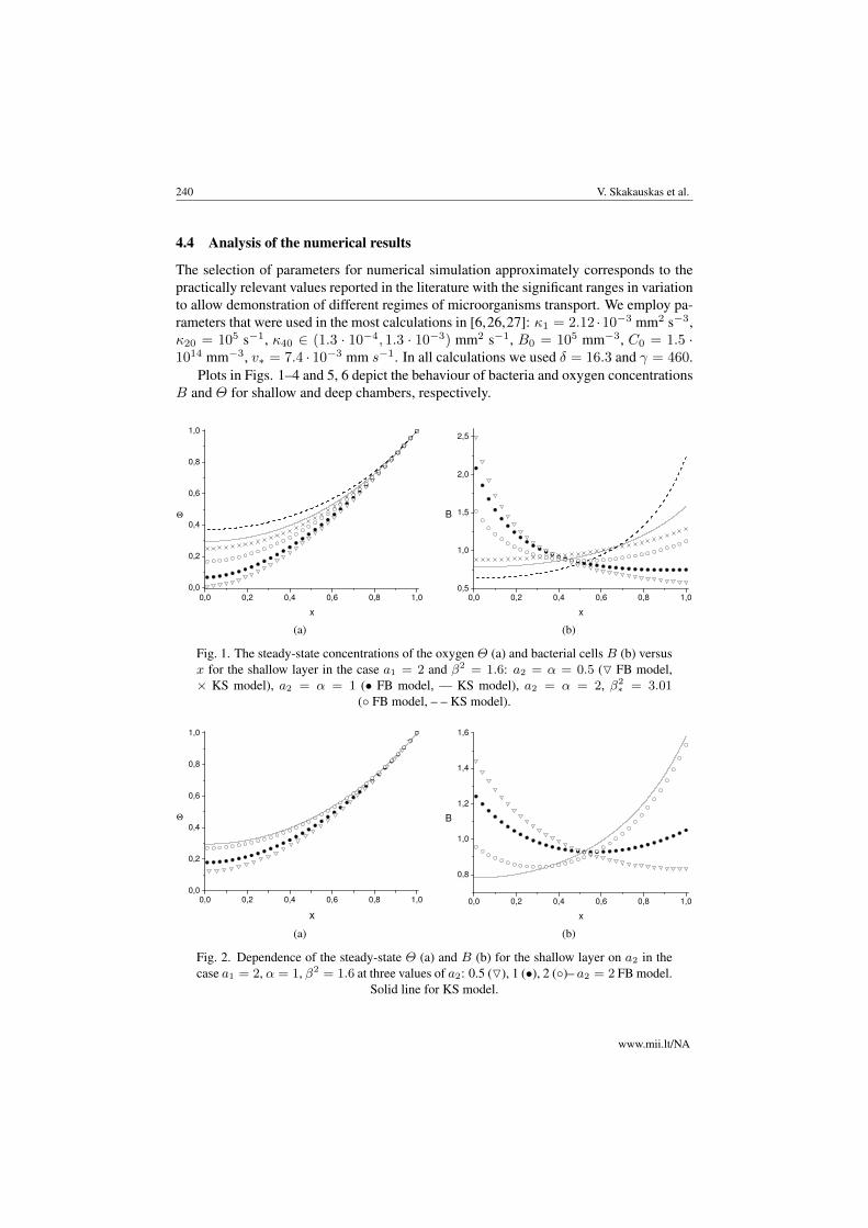
Fig. 1. The steady-state concentrations of the oxygen Θ (a) and bacterial cells B (b) versusx for the shallow layer in the case a1 = 2 and β2 = 1.6: a2 = α = 0.5 (O FB model,× KS model), a2 = α = 1 (• FB model, — KS model), a2 = α = 2, β2

∗ = 3.01(◦ FB model, – – KS model).

0,0 0,2 0,4 0,6 0,8 1,0

0,0

0,2

0,4

0,6

0,8

1,0

Θ

x

(a)

0,0 0,2 0,4 0,6 0,8 1,0

0,8

1,0

1,2

1,4

1,6

B

x

(b)

Fig. 2. Dependence of the steady-state Θ (a) and B (b) for the shallow layer on a2 in thecase a1 = 2, α = 1, β2 = 1.6 at three values of a2: 0.5 (O), 1 (•), 2 (◦)– a2 = 2 FB model.

Solid line for KS model.

www.mii.lt/NA


0,0 0,2 0,4 0,6 0,8 1,0

0,0

0,2

0,4

0,6

0,8

1,0

Θ

x

(a)

0,0 0,2 0,4 0,6 0,8 1,0

1,0

1,5

2,0

B

x

(b)

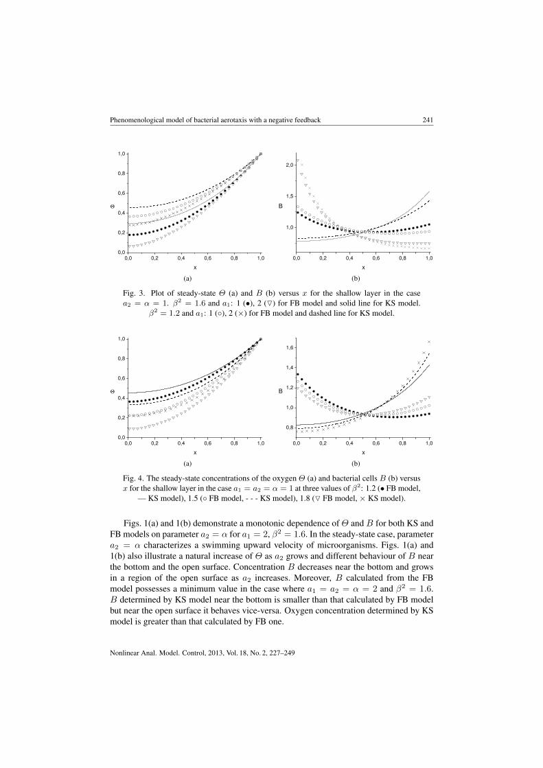
Fig. 3. Plot of steady-state Θ (a) and B (b) versus x for the shallow layer in the casea2 = α = 1. β2 = 1.6 and a1: 1 (•), 2 (O) for FB model and solid line for KS model.

β2 = 1.2 and a1: 1 (◦), 2 (×) for FB model and dashed line for KS model.

0,0 0,2 0,4 0,6 0,8 1,0

0,0

0,2

0,4

0,6

0,8

1,0

Θ

x

(a)

0,0 0,2 0,4 0,6 0,8 1,0

0,8

1,0

1,2

1,4

1,6

B

x

(b)

Fig. 4. The steady-state concentrations of the oxygen Θ (a) and bacterial cells B (b) versusx for the shallow layer in the case a1 = a2 = α = 1 at three values of β2: 1.2 (• FB model,

— KS model), 1.5 (◦ FB model, - - - KS model), 1.8 (O FB model, × KS model).

Figs. 1(a) and 1(b) demonstrate a monotonic dependence of Θ and B for both KS andFB models on parameter a2 = α for a1 = 2, β2 = 1.6. In the steady-state case, parametera2 = α characterizes a swimming upward velocity of microorganisms. Figs. 1(a) and1(b) also illustrate a natural increase of Θ as a2 grows and different behaviour of B nearthe bottom and the open surface. Concentration B decreases near the bottom and growsin a region of the open surface as a2 increases. Moreover, B calculated from the FBmodel possesses a minimum value in the case where a1 = a2 = α = 2 and β2 = 1.6.B determined by KS model near the bottom is smaller than that calculated by FB modelbut near the open surface it behaves vice-versa. Oxygen concentration determined by KSmodel is greater than that calculated by FB one.



0,0 0,2 0,4 0,6 0,8 1,0

0,0

0,2

0,4

0,6

0,8

1,0

Θ

x

(a)

0,0 0,2 0,4 0,6 0,8 1,0

0,6

0,8

1,0

1,2

1,4

1,6

1,8

2,0

2,2

B

x

(b)

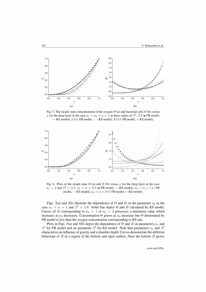
Fig. 5. The steady-state concentrations of the oxygen Θ (a) and bacterial cells B (b) versusx for the deep layer in the case a1 = a2 = α = 1 at three values of β2: 2.5 (• FB model,

— KS model), 3.5 (◦ FB model, - - - KS model), 4.5 (O FB model, × KS model).

0,0 0,2 0,4 0,6 0,8 1,0

0,0

0,2

0,4

0,6

0,8

1,0

Θ

x

(a)

0,0 0,2 0,4 0,6 0,8 1,0

0,5

1,0

1,5

2,0

2,5

B

x

(b)

Fig. 6. Plots of the steady-state Θ (a) and B (b) versus x for the deep layer in the casea1 = 2 and β2 = 3.5: a2 = α = 0.5 (• FB model, — KS model), a2 = α = 1 (◦ FB

model, - - KS model), a2 = α = 2 (O FB model, × KS model).

Figs. 2(a) and 2(b) illustrate the dependence of Θ and B on the parameter a2 in thecase a1 = α = 1 and β2 = 1.6. Solid line depict Θ and B calculated by KS model.Curves of B corresponding to a2 = 1 or a2 = 2 possesses a minimum value whichincreases as a2 decreases. Concentration Θ grows as a2 increases but Θ determined byFB model is less than the oxygen concentration corresponding to KS one.

Plots in Figs. 3(a) and 3(b) depict the dependence of Θ and B on parameters a1 andβ2 for FB model and on parameter β2 for KS model. Note that parameters a1 and β2

characterize an influence of gravity and a chamber depth. Curves demonstrate the differentbehaviour of B in a region of the bottom and open surface. Near the bottom B grows

www.mii.lt/NA


as a1 increases but far from the bottom it behaves vice-versa. Figure also demonstrates thedifferent behaviour ofB determined by both KS and FB models. Oxygen concentrationΘdecreases for all x as a1 or β2 increases.

Plots in Figs. 4(a) and 4(b) depict the dependence of Θ and B on parameter β2 forboth KS and FB models and demonstrate their monotonic behaviour as β2 grows. Valuesof B that correspond to KS and FB models near the bottom are larger than correspondingones near the open surface. Values of Θ determined by KS model for all x are larger thatthose corresponding with FB model.

Figs. 5(a) and 5(b), 6(a) and 6(b) demonstrate the dependence of Θ and B on param-eters β2 and a2, respectively, for a deep chamber. We observe a monotonic behaviourof B for both KS and FB models with respect to parameter β2. But this behaviour issimilar near the bottom and the open surface and is different in the intermediate region(see Figs. 5(a) and 5(b)). The qualitative behaviour of B and Θ with respect to a2 issimilar to that of the shallow chamber (see Figs. 6(a) and 6(b)).

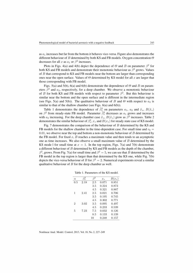
Table 1 demonstrates the dependence of β̃2∗ on parameters a1, a2 and x̃∗, B(x̃∗)

on β2 from steady-state FB model. Parameter β̃2∗ decreases as a1 grows and increases

with a2 increasing. For the deep chamber case x̃∗, B(x̃∗) grow as β2 increases. Table 2demonstrates the similar behaviour of β2

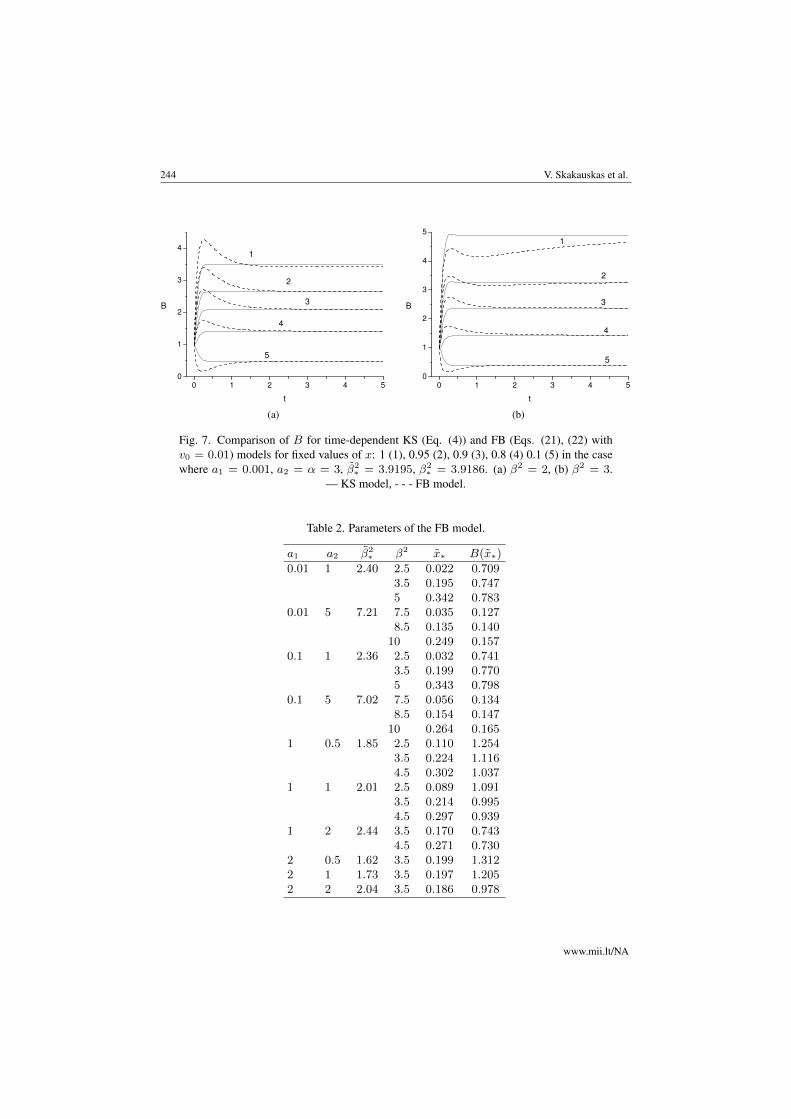
∗ , x∗ andB(x∗) for steady state case of KS model.Fig. 7 demonstrates the comparison of the behaviour of B determined by the KS and

FB models for the shallow chamber in the time-dependent case. For small time and v0 =0.01, we observe near the top and bottom a non-monotonic behaviour ofB determined bythe FB model. For fixed x, B reaches a maximum value and then tends to an asymptoticone as time increases. We also observe a small maximum value of B determined by theKS mode l for small time at x = 1. In the top region, Figs. 7(a) and 7(b) demonstratea different behaviour of B determined by KS and FB models as the depth of the chamber,β2, grows. From Fig. 7(a) for small time and β2 = 5, we can see thatB determined by theFB model in the top region is larger than that determined by the KS one, while Fig. 7(b)depicts the vice-versa behaviour of B for β2 = 2. Numerical experiments reveal a similarqualitative behaviour of B for the deep chamber as well.

Table 1. Parameters of the KS model.

α β2∗ β2 x∗ B(x∗)

0.5 2.18 2.5 0.071 0.8513.5 0.224 0.8734.5 0.321 0.887

1 2.41 2.5 0.021 0.7063.5 0.195 0.7454.5 0.302 0.771

2 3.02 3.5 0.095 0.4974.5 0.233 0.539

5 7.23 7.5 0.032 0.1268.5 0.133 0.139

10 0.248 0.157



0 1 2 3 4 5

0

1

2

3

4

5

4

3

2

B

t

1

(a)

0 1 2 3 4 5

0

1

2

3

4

5

5

4

3

2

B

t

1

(b)

Fig. 7. Comparison of B for time-dependent KS (Eq. (4)) and FB (Eqs. (21), (22) withv0 = 0.01) models for fixed values of x: 1 (1), 0.95 (2), 0.9 (3), 0.8 (4) 0.1 (5) in the casewhere a1 = 0.001, a2 = α = 3, β̃2

∗ = 3.9195, β2∗ = 3.9186. (a) β2 = 2, (b) β2 = 3.

— KS model, - - - FB model.

Table 2. Parameters of the FB model.

a1 a2 β̃2∗ β2 x̃∗ B(x̃∗)

0.01 1 2.40 2.5 0.022 0.7093.5 0.195 0.7475 0.342 0.783

0.01 5 7.21 7.5 0.035 0.1278.5 0.135 0.140

10 0.249 0.1570.1 1 2.36 2.5 0.032 0.741

3.5 0.199 0.7705 0.343 0.798

0.1 5 7.02 7.5 0.056 0.1348.5 0.154 0.147

10 0.264 0.1651 0.5 1.85 2.5 0.110 1.254

3.5 0.224 1.1164.5 0.302 1.037

1 1 2.01 2.5 0.089 1.0913.5 0.214 0.9954.5 0.297 0.939

1 2 2.44 3.5 0.170 0.7434.5 0.271 0.730

2 0.5 1.62 3.5 0.199 1.3122 1 1.73 3.5 0.197 1.2052 2 2.04 3.5 0.186 0.978

www.mii.lt/NA


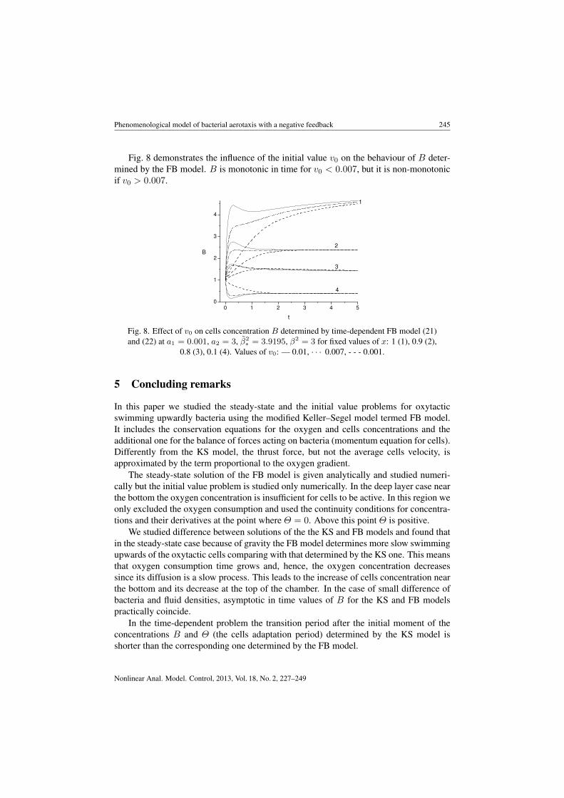
Fig. 8 demonstrates the influence of the initial value v0 on the behaviour of B deter-mined by the FB model. B is monotonic in time for v0 < 0.007, but it is non-monotonicif v0 > 0.007.

0 1 2 3 4 5

0

1

2

3

4

4

3

2

B

t

1

Fig. 8. Effect of v0 on cells concentration B determined by time-dependent FB model (21)and (22) at a1 = 0.001, a2 = 3, β̃2

∗ = 3.9195, β2 = 3 for fixed values of x: 1 (1), 0.9 (2),0.8 (3), 0.1 (4). Values of v0: — 0.01, · · · 0.007, - - - 0.001.

5 Concluding remarks

In this paper we studied the steady-state and the initial value problems for oxytacticswimming upwardly bacteria using the modified Keller–Segel model termed FB model.It includes the conservation equations for the oxygen and cells concentrations and theadditional one for the balance of forces acting on bacteria (momentum equation for cells).Differently from the KS model, the thrust force, but not the average cells velocity, isapproximated by the term proportional to the oxygen gradient.

The steady-state solution of the FB model is given analytically and studied numeri-cally but the initial value problem is studied only numerically. In the deep layer case nearthe bottom the oxygen concentration is insufficient for cells to be active. In this region weonly excluded the oxygen consumption and used the continuity conditions for concentra-tions and their derivatives at the point where Θ = 0. Above this point Θ is positive.

We studied difference between solutions of the the KS and FB models and found thatin the steady-state case because of gravity the FB model determines more slow swimmingupwards of the oxytactic cells comparing with that determined by the KS one. This meansthat oxygen consumption time grows and, hence, the oxygen concentration decreasessince its diffusion is a slow process. This leads to the increase of cells concentration nearthe bottom and its decrease at the top of the chamber. In the case of small difference ofbacteria and fluid densities, asymptotic in time values of B for the KS and FB modelspractically coincide.

In the time-dependent problem the transition period after the initial moment of theconcentrations B and Θ (the cells adaptation period) determined by the KS model isshorter than the corresponding one determined by the FB model.



We hope that the model of the FB type with an additional term of bacteria to bacteriacommunication in the differential equation for v could be regarded as phenomenologicaleffective one to capture the possible variability of the oxytactic bacteria response to theenvironmental changes in real systems.

Appendix

To find the numerical solution of problem (21) and (22) the finite-difference scheme wasused.

Assume that tj = jτ , 0 6 j 6 M , τ = T/M , xi = ih, 0 6 i 6 N , h = 1/N . Setθji = θ(tj , xi), bji = b(tj , xi), vji = v(tj , xi).

Approximating the differential equations (21) with an implicit scheme the followingfinite difference equations are obtained:

θj+1i − θjiτ

= δ

(θj+1i−1 − 2θj+1

i + θj+1i+1

h2− β2bji

),

bj+1i − bjiτ

=bj+1i−1 − 2bj+1

i + bj+1i+1

h2− γ

vji+1bji+1 − v

ji−1b

ji−1

2h,

bjivj+1i − vjiτ

=ρ3γ

(−a1bji + a2

θji+1 − θji−1

2h− γvji

),

i = 1, 2, . . . , N − 1; j = 0, 1, . . . ,M − 1.

(A.1)

The boundary and initial conditions (22) are approximated by

bj+11 − bj+1

0

h− γ v

j1bj1 + vj0b

j0

2= 0,

bj+1N − bj+1

N−1h

− γvjN−1b

jN−1 + vjNb

jN

2= 0,

θj+11 = θj+1

0 , θj+1N = 1,

θ0i = 1, b0i = 1, v0i = v0,

i = 0, 1, . . . , N ; j = 0, 1, . . . ,M − 1.

(A.2)

To get the discrete form of Eq. (21)3 at x = 0 and 1 we use the difference equations

bj0vj+10 − vj0τ

=ρ3γ

(−a1bj0 − γv

j0

),

bjNvj+1N − vjN

τ=ρ3γ

(−a1bjN + a2

θjN − θjN−1

h− γvjN

),

j = 0, 1, . . . ,M − 1.

(A.3)

www.mii.lt/NA


To write the difference scheme to KS model the following approximation of (4)2 andboundary conditions for function B instead of Eqs. (A.1)2 and (A.2)1,2 are used:

bj+1i − bjiτ

=bj+1i−1 − 2bj+1

i + bj+1i+1

h2

−αh

(bji+1 + bji

2

θji+1 − θji

h−bji + bji−1

2

θji − θji−1

h

),

i = 1, 2, . . . , N − 1; j = 0, 1, . . . ,M − 1,

(A.4)

bj+11 = bj+1

0 ,

bj+1N − bjN−1

h− α

bjN−1 + bjN2

θjN − θjN−1

h= 0,

j = 0, 1, . . . ,M − 1.

(A.5)

From (A.1)2, (A.2)1,2 or (A.4), (A.5) the discrete analogue of condition (6)h∑N−1i=1 bj+1

i = h∑N−1i=1 bji , j = 0, 1, . . . ,M − 1, follows.

References

1. E.F. Keller, L.A. Segel, Model for chemotaxis, J. Theor. Biol., 30:225–234, 1971.

2. E.F. Keller, L.A. Segel, Travelling bands of chemotaxis bacteria, J. Theor. Biol., 30:235–248,1971.

3. D. Horstmann, From 1970 until present: The Keller–Segel model in chemotaxis and itsconsequences. I, Jahresberichte DMV, 105(3):103–165, 2003.

4. T. Hillen, K.J. Painter, A user’s guide to PDE models for chemotaxis, J. Math. Biol., 58:183–217, 2009.

5. N.A. Hill, T.J. Pedley, Bioconvection, Fluid Dyn. Res., 37:1–20, 2005.

6. A.J. Hillesdon, T.J. Pedley, J.O. Kessler, The development of concentration gradients ina suspension of chemotactic bacteria, Bull. Math. Biol., 57(2):299–344, 1995.

7. A.J. Hillesdon, T.J. Pedley, Bioconvection in suspensions of oxytactic bacteria: Linear theory,J. Fluid Mech., 324:223–259, 1996.

8. C. Dombrowski, L. Cisneros, S. Shatkaew, R. Goldstein, J. Kessler, Self-concentration andlarge-scale coherence in bacterial dynamics, Phys. Rev. Lett., 93, 098103, 2004.

9. I. Tuval, L. Cisneros, C. Dombrowski, C. Wolgemuth, J. Kessler, R. Goldstein, Bacterialswimming and oxygen transport near contact lines, Proc. Natl Acad. Sci., 102:2277–2282,2005.

10. A. Chertock, K. Fellner, A. Kurganov, A. Lorz, P.A. Markowich, Sinking, merging andstationary plumes in a coupled chemotaxis-fluid model: A high-resolution numerical approach,J. Fluid Mech., 694:155–190, 2012.



11. A. Lorz, Coupled chenmotaxis fluid model, Math. Models Meth. Appl. Sci., 20:1–17, 2010.

12. R.-J. Duan, A. Lorz, P. Markovich, Global solutions to the coupled chemotaxis-fluid equations,Commun. Part. Diff. Equ., 35:1–39, 2010.

13. M. Di Francesco, A. Lorz, P. Markovich, Chemotaxis-fluid coupled model for swimmingbacteria with nonlinear diffusion: Global existence and asymptotic behaviour, Discrete Contin.Dyn. Syst. A, 28(4):1437–1453, 2010.

14. S.M. Becker, A.V. Kuznetsov, A.A. Avramenko, Numerical modelling of a falling biocon-vection plume in a porous medium, Fluid Dyn. Res., 33:323–339, 2004.

15. A.V. Kuznetsov, A.A. Avramenko, Analysis of stability of bioconvection of motile oxytacticbacteria in a horizontal fluid saturated porous layer, Int. Commun. Heat Mass Transfer, 30:593–602, 2003.

16. A.V. Kuznetsov, A.A. Avramenko, P. Geng, Analytical investigation of a falling plume causedby bioconvection of oxytactic bacteria in a fluid saturated porous medium, Int. J. Eng. Sci.,42:557–569, 2004.

17. A.V. Kuznetsov, Thermo-bioconvection in a suspension of oxytactic bacteria, Int. Commun.Heat Mass Transfer, 32:991–999, 2005.

18. A.V. Kuznetsov, Investigation of the onset of thermo-bioconvection in a suspension of oxytacticmicroorganisms in a shallow fluid layer heated from below, Theor. Comput. Fluid. Dyn.,19(4):287–299, 2005.

19. A.V. Kuznetsov, The onset of thermo-bioconvection in a shallow fluid saturated porous layerheated from below in a suspension of oxytactic microorganisms, Eur. J. Mech. B Fluids,25:223–233, 2006.

20. Z. Alloui, T.H. Nguyen, E. Bilgen, Bioconvection of gravitactic microorganisms in a verticalcylinder, Int. J. Heat Mass Transfer, 32:739–747, 2005.

21. Z. Alloui, T.H. Nguyen, E. Bilgen, Numerical investigation of thermo-bioconvection in a sus-pension of gravitactic microorganisms, Int. J. Heat Mass Transfer, 50:1435–1441, 2007.

22. Z. Alloui, T.H. Nguyen, E. Bilgen, Stability analysis of thermo-bioconvection in suspensions ofgravitactic microorganisms in a fluid layer, Int. Commun. Heat Mass Transfer, 33:1198–1206,2006.

23. M.A. Herrero, J.J.L. Velazquez, Chemotactic collapse for the Keller–Segel model, J. Math.Biol., 35:177–194, 1996.

24. B.L. Taylor, I.B. Zhulin, M.S. Johnson, Aerotaxis and other energy sensing behavior in bac-teria, Ann. Rev. Microbiol., 53:103–128, 1999.

25. J. Shioi, C.V. Dang, B.L. Taylor, Oxygen as attractant and repellent in bacterial chemotaxis,J. Bacteriol., 169(7):3118–3123, 1987.

26. R. Baronas, R. Šimkus, Modeling the bacterial self-organization in a circular container alongthe contact line as detected by bioluminescence imaging, Nonlinear Anal. Model. Control,16(3):270–282, 2011.

www.mii.lt/NA


27. R. Šimkus, R. Baronas, Metabolic self-organization of bioluminescent Escherichia coli,Luminescence, 26(6):716–721, 2011.

28. M. Eisenbach, Chemotaxis, Imperial College Press, London, 2004.

29. R.M. Macnab, D.E. Koshland, Jr., The gradient-sensing mechanism in bacerial chemotaxis,Proc. Nat. Acad. Sci. USA, 69(9):2509–2512, 1972.

30. H.G. Othmer, T. Hillen, The diffusion limit of transport equations II: Chemotaxis equations,SIAM J. Appl. Math., 62(4):1222–1250, 2002.

31. T. Hillen, K. Painter, C. Schmeiser, Global existence for chemotaxis with finite sampling radius,Discr. Cont. Dyn. Syst. B, 7(1):125–144, 2007.

32. A.A. Samarskii, The Theory of Difference Schemes, Marcel Dekker, New York, 2001.


Documents

Phenomenological model of bacterial aerotaxis with a