PHENOMENA THAT DETERMINE KNOCK ONSET IN SPARK …

PHENOMENA THAT DETERMINEKNOCK ONSET IN SPARK-IGNITED ENGINES

by

Bridget M. Revier

B.S., Chemical EngineeringB.S., Chemistry

Rose-Hulman Institute of Technology, 2004

Submitted to the Department of Mechanical Engineeringin Partial Fulfillment of the Requirements for the Degree of

Master of Science in Mechanical Engineering

at the

Massachusetts Institute of Technology

June 2006

0 2006 Massachusetts Institute of TechnologyAll Rights Reserved

Signature of the A uthor ................................ r . ....... .. . .. ... ........Departn of Mechanical Engineering

May 17, 2006

C ertified b y .................................................................... ....-- -- -- -John B. Heywood

Sun Jae Professor of Mechanical EngineeringThesis Advisor

A ccepted by.......................................

ASSACHUSETTS INSTITUTE ProfeOF TECHNOLOGY Ch

JU L 14 2006 BARKER

LIBRARIES

Lallit Anandssor, Department of Mechanical Engineeringairman, Department of Graduate Committee

M

(page intentionally left blank)

2

PHENOMENA THAT DETERMINEKNOCK ONSET IN SPARK-IGNITED ENGINES

by

Bridget M. Revier

Submitted to the Department of Mechanical Engineeringon May 17, 2006 in Partial Fulfillment of the

Requirements for the Degree of Master of Science inMechanical Engineering

ABSTRACT

Experiments were carried out to collect in-cylinder pressure data and microphone signalsfrom a single-cylinder test engine using spark timings before, at, and after knock onsetfor four different octane-rated toluene reference fuels. This data was then processed andanalyzed in various ways to gain insight into the autoignition phenomena that lead toknock. This was done to develop a more fundamentally based prediction methodologythat incorporates both a physical and chemical description of knock. The collected datawas also used to develop a method of data processing that would detect knock in realtime without the need to have an operator listening to the engine.

Bandpass filters and smoothing techniques were used to process the data. The processeddata was then used to determine knock intensities for each cycle for both the cylinderpressure data and microphone signal. Also, the rate of build-up before reaching peakamplitude in a bandpass filtered pressure trace was found. A trend was found showingthat cycles with knock intensities greater than 1 bar with rapid build-up (5-10oscillations) before reaching the peak are the type the cycles whose autoignition eventslead to engine knock. The cylinder pressure knock intensities and microphone knockintensities were plotted and then fit with a linear trendline. The R2 value for these lineartrendlines will transition from considerably lower values to values greater than 0.85 at thespark timing of knock onset.

It is believed that the higher cylinder pressure knock intensities, in conjunction with thefaster build-up of 5-10 oscillations before reaching peak, helps to explain the knockphenomena. It supports conclusions from previous works that the end gas contains oneor more hot spots that autoignite in sequence causing pressure gradients that can triggerrapid pressure oscillations. These pressure oscillations can cause block and headvibrations that lead to audible noise outside the engine

Thesis Advisor: John B. HeywoodTitle: Sun Jae Professor of Mechanical Engineering

3


4

I would like to thank my friends, family, and coworkersfor the great deal of support they have provided me

throughout this endeavor.

5


6

TABLE OF CONTENTS

A B S T R A C T ........................................................................................................................ 3TABLE OF CONTENTS ................................................................................................ 7L IST O F T A B L E S ......................................................................................................... . 9L IST O F FIG U R E S .......................................................................................................... 11

CHAPTER 1: INTRODUCTION ................................................................................. 131.1 KNOCK FUNDAMENTALS............................................................................. 13

1.1.1 K nock D efinition ........................................................................................... 131.1.2 Factors that Affect Engine Knock................................................................. 14

1.2 PR EV IO U S W O R K .............................................................................................. 151.2.1 Brief Overview of Knock Detection Methods ............................................. 151.2.2 Variation in Levels of Pressure Waves ......................................................... 161.2.3 Proposed Mechanisms for the Increase in Pressure Oscillation Amplitude .... 17

1.3 RESEARCH OBJECTIVES............................................................................... 20

CHAPTER 2: EXPERIMENTAL METHOD .............................................................. 212.1 TEST CELL SETUP........................................................................................... 21

2.1.1 Engine Specifications.................................................................................... 212.1.2 Dynamometer Specifications ........................................................................ 21

2.1.3 A ir and Fuel System s .................................................................................... 222.2 ENGINE CONTROL AND MEASUREMENTS ............................................... 23

2.2.1 Engine C ontrol U nit...................................................................................... 232.2.2 Intake Pressure Control and Measurement .................................................. 24

2.2.3 Temperature Control and Measurement ...................................................... 24

2.2.4 Air Flow Measurement ................................................................................. 24

2.2.5 Fuel Flow Measurement ............................................................................... 24

2.2.6 Air-Fuel Ratio Measurement ....................................................................... 252.2.7 Cylinder Pressure Measurement ................................................................... 252.2.8 K nock D etection ........................................................................................... 252.2.9 Microphone Measurement ............................................................................ 26

2.3 EXPERIMENTAL PROCEDURES AND INFORMATION ............................ 262.3.1 Experimental Procedure............................................................................... 262.3.2 Experimental Fuels ...................................................................................... 27

CHAPTER 3: DATA AND DATA PROCESSING METHODS.................................. 293.1 D A T A SE T S ...................................................................................................... . 29

3.1.1 Experimental Conditions .............................................................................. 293.1.2 F ilter Param eters .......................................................................................... . 303.1.3 Smoothing Technique ................................................................................... 313.1.4 Microphone Signal Processing ..................................................................... 32

3.2 DATA PROCESSING AND ANALYZATION ................................................. 333.2.1 Determining the Cylinder Pressure Signal Frequencies .............................. 33

3.2.2 Knock Indications in Filtered Cylinder Pressure Signal............................... 35

3.2.3 Data Analysis Method for Cylinder Pressure without Filtering ................... 42

7

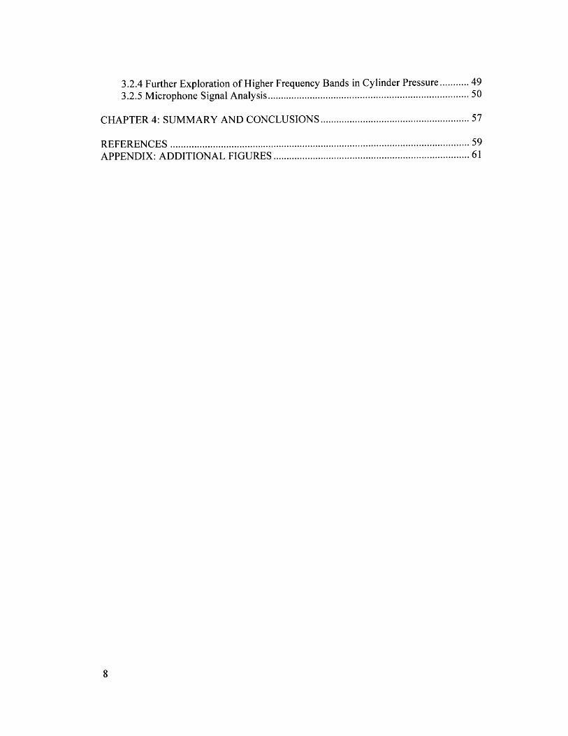
3.2.4 Further Exploration of Higher Frequency Bands in Cylinder Pressure........ 49

3.2.5 M icrophone Signal A nalysis........................................................................ 50

CHAPTER 4: SUMMARY AND CONCLUSIONS.................................................... 57

R E F E R E N C E S ................................................................................................................. 59APPENDIX: ADDITIONAL FIGURES ...................................................................... 61

8

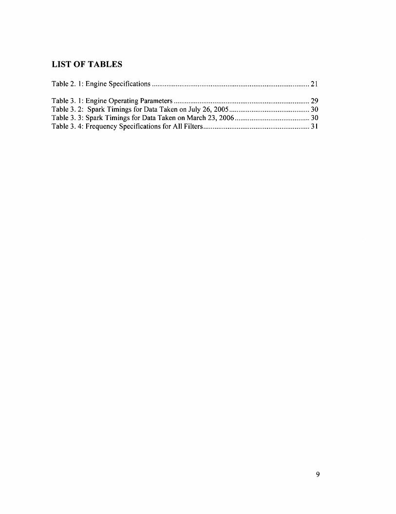
LIST OF TABLES

Table 2. 1: Engine Specifications ................................................................................. 21

Table 3. 1: Engine Operating Parameters ..................................................................... 29Table 3. 2: Spark Timings for Data Taken on July 26, 2005........................................ 30Table 3. 3: Spark Timings for Data Taken on March 23, 2006................................... 30Table 3. 4: Frequency Specifications for All Filters.................................................... 31

9


10

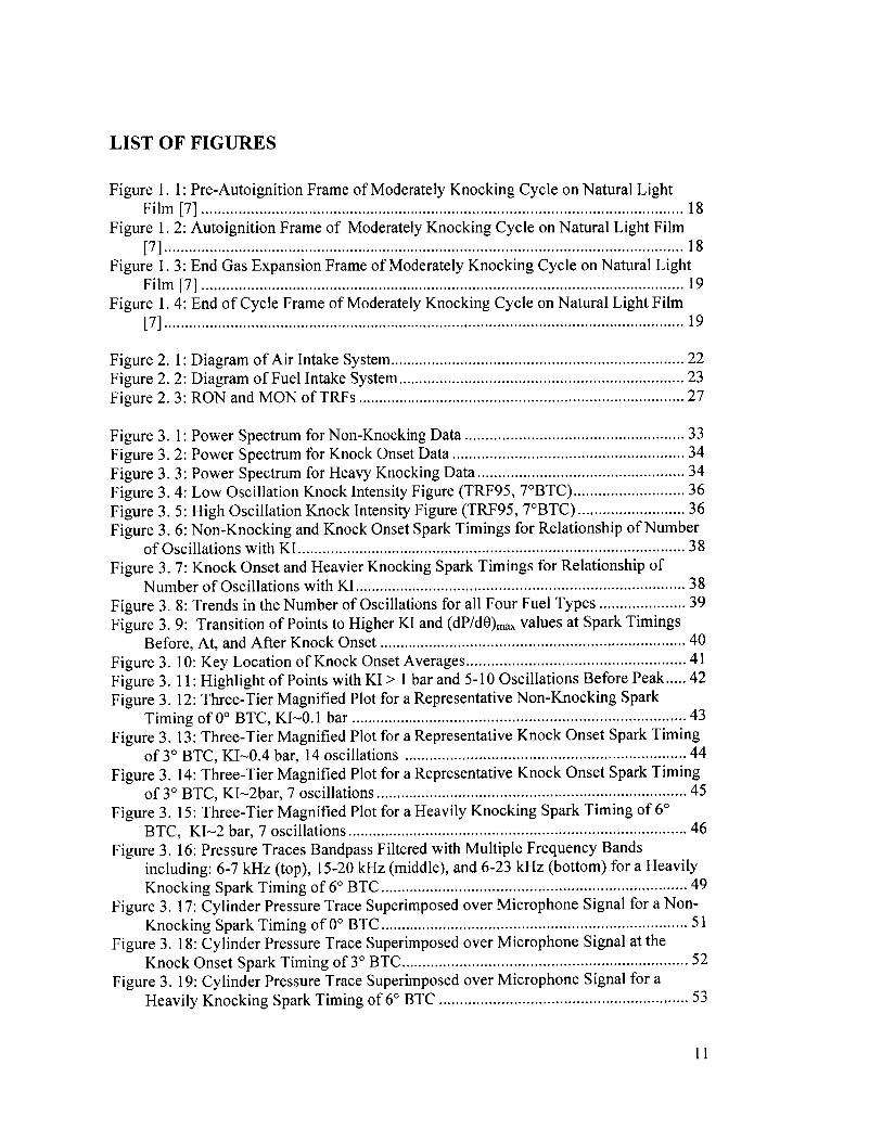
LIST OF FIGURES

Figure 1. 1: Pre-Autoignition Frame of Moderately Knocking Cycle on Natural LightF ilm [7 ] ..................................................................................................................... 18

Figure 1. 2: Autoignition Frame of Moderately Knocking Cycle on Natural Light Film[7 ] .............................................................................................................................. 1 8

Figure 1. 3: End Gas Expansion Frame of Moderately Knocking Cycle on Natural LightF ilm [7 ] ..................................................................................................................... 19

Figure 1. 4: End of Cycle Frame of Moderately Knocking Cycle on Natural Light Film[7 ] .............................................................................................................................. 19

Figure 2. 1: Diagram of Air Intake System ................................................................... 22Figure 2. 2: Diagram of Fuel Intake System ................................................................. 23Figure 2. 3: RON and M ON of TRFs .......................................................................... 27

Figure 3. 1: Power Spectrum for Non-Knocking Data .................................................. 33Figure 3. 2: Power Spectrum for Knock Onset Data .................................................... 34Figure 3. 3: Power Spectrum for Heavy Knocking Data ............................................. 34Figure 3. 4: Low Oscillation Knock Intensity Figure (TRF95, 70BTC)....................... 36Figure 3. 5: High Oscillation Knock Intensity Figure (TRF95, 70BTC)...................... 36Figure 3. 6: Non-Knocking and Knock Onset Spark Timings for Relationship of Number

of O scillations w ith K I........................................................................................... 38Figure 3. 7: Knock Onset and Heavier Knocking Spark Timings for Relationship of

N um ber of O scillations w ith K I............................................................................. 38Figure 3. 8: Trends in the Number of Oscillations for all Four Fuel Types ................. 39Figure 3. 9: Transition of Points to Higher KI and (dP/dO)max values at Spark Timings

Before, At, and A fter Knock Onset ....................................................................... 40Figure 3. 10: Key Location of Knock Onset Averages.................................................. 41Figure 3. 11: Highlight of Points with KI > 1 bar and 5-10 Oscillations Before Peak..... 42Figure 3. 12: Three-Tier Magnified Plot for a Representative Non-Knocking Spark

Tim ing of 00 BTC, K I-0. 1 bar ............................................................................ 43Figure 3. 13: Three-Tier Magnified Plot for a Representative Knock Onset Spark Timing

of 30 BTC, KI-0.4 bar, 14 oscillations ............................................................... 44Figure 3. 14: Three-Tier Magnified Plot for a Representative Knock Onset Spark Timing

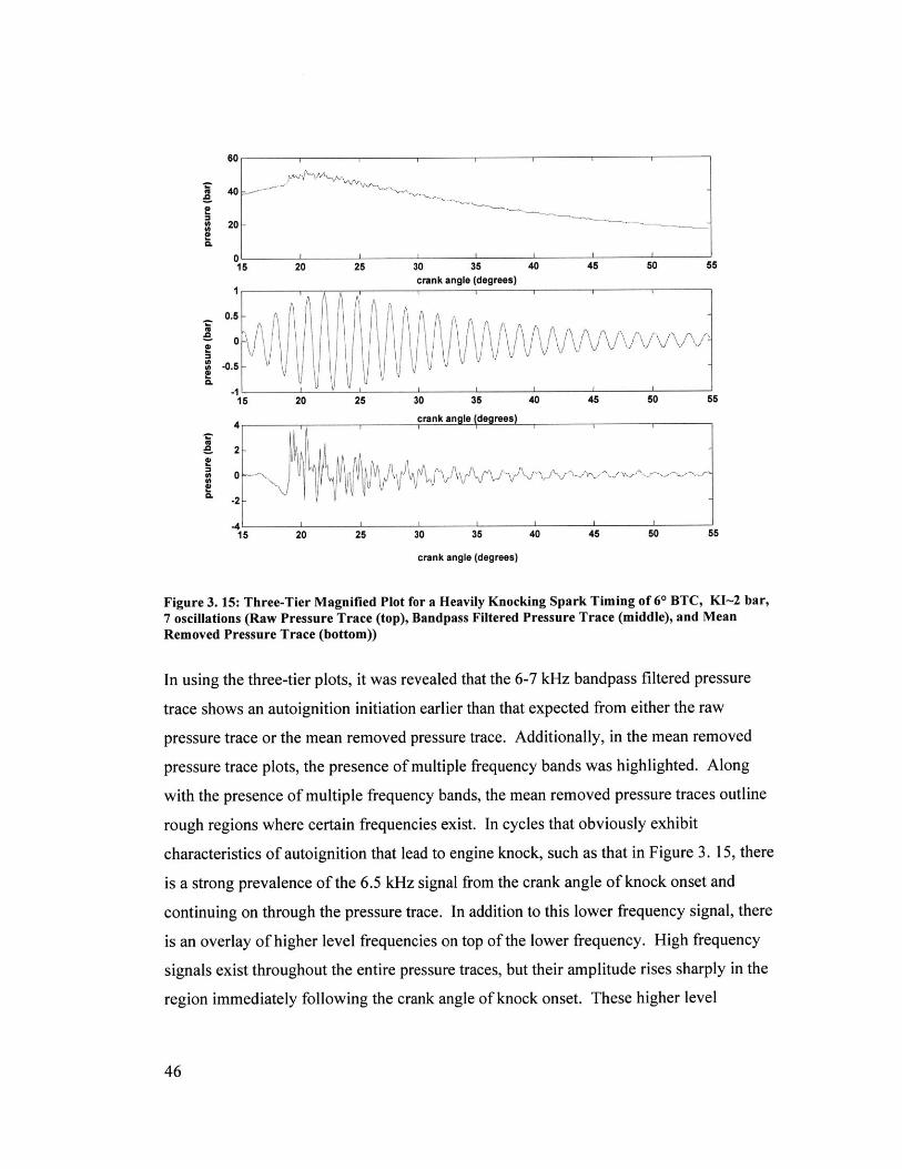
of 30 BTC, KI-2bar, 7 oscillations ....................................................................... 45Figure 3. 15: Three-Tier Magnified Plot for a Heavily Knocking Spark Timing of 60

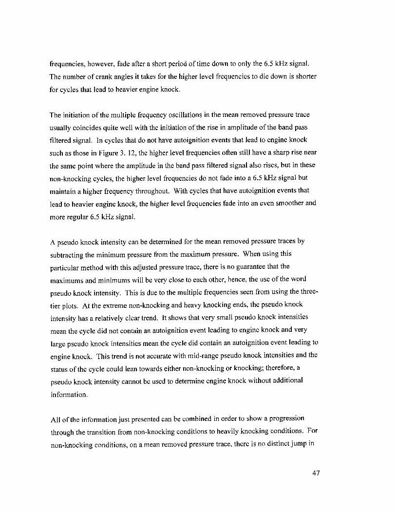
B TC , K I-2 bar, 7 oscillations ............................................................................... 46Figure 3. 16: Pressure Traces Bandpass Filtered with Multiple Frequency Bands

including: 6-7 kHz (top), 15-20 kHz (middle), and 6-23 kHz (bottom) for a HeavilyKnocking Spark Tim ing of 60 BTC..................................................................... 49

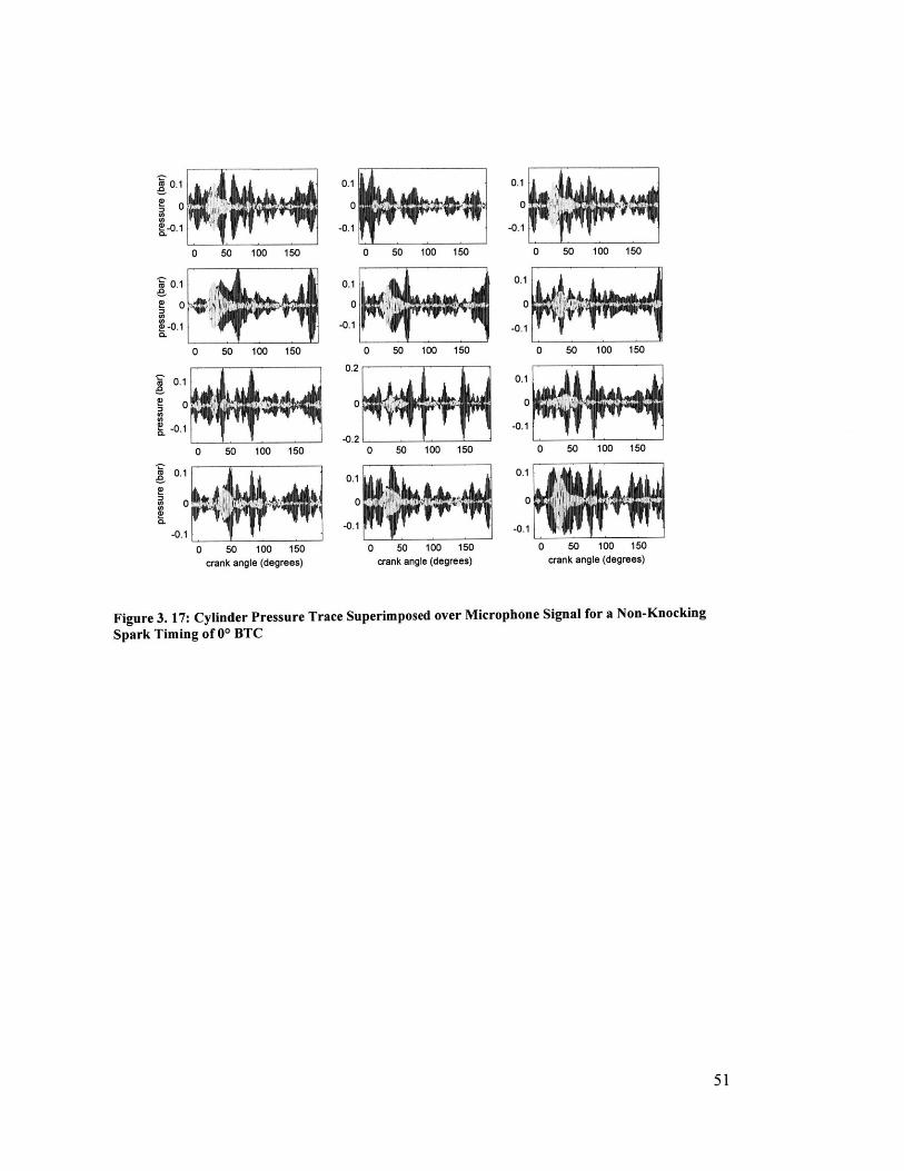
Figure 3. 17: Cylinder Pressure Trace Superimposed over Microphone Signal for a Non-Knocking Spark Tim ing of 00 BTC ....................................................................... 51

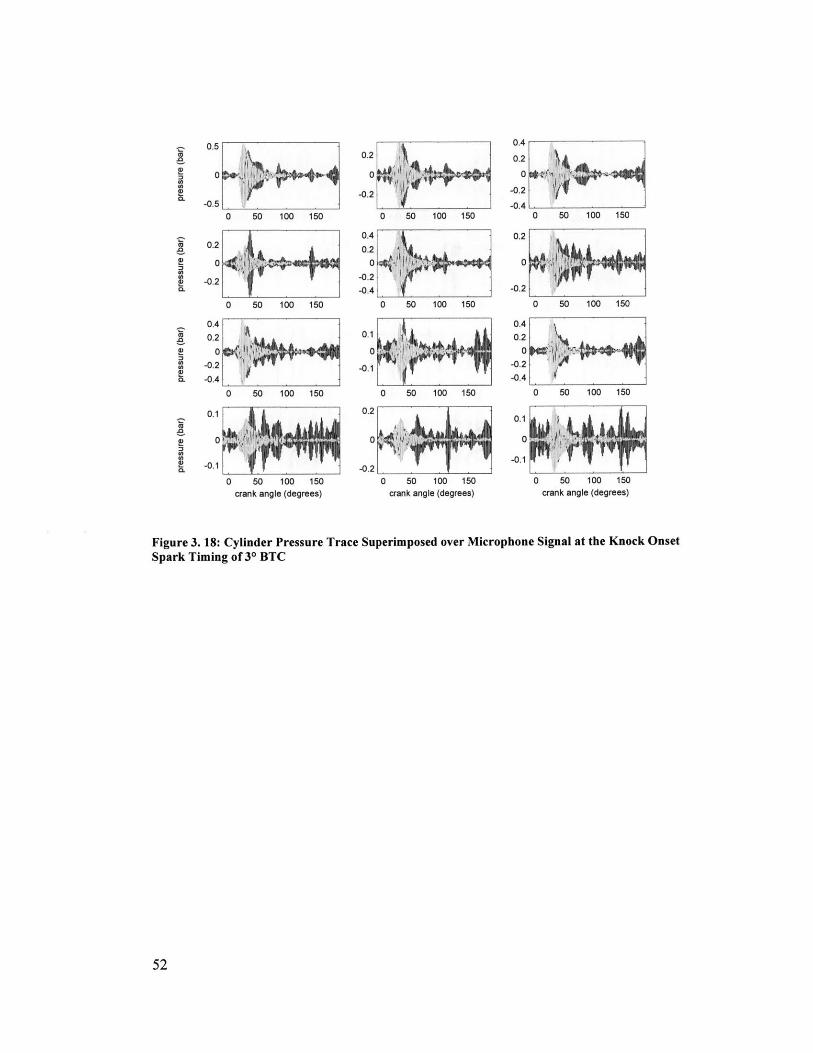
Figure 3. 18: Cylinder Pressure Trace Superimposed over Microphone Signal at theKnock Onset Spark Timing of 30 BTC................................................................ 52

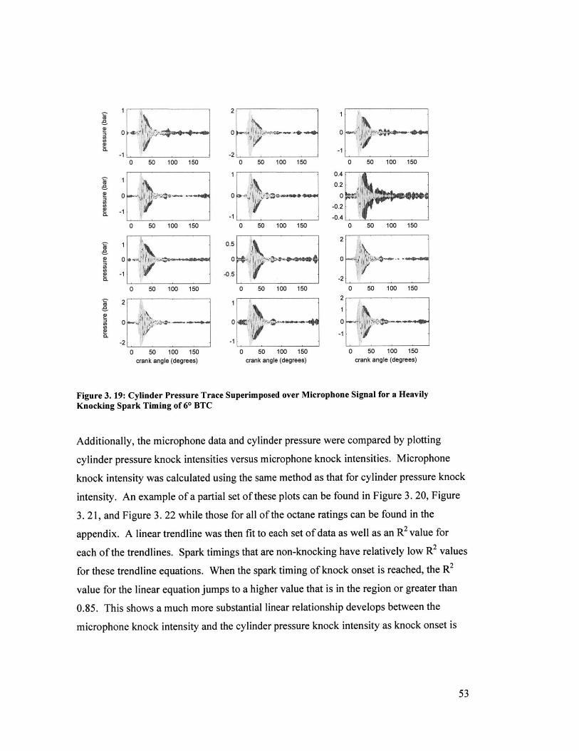
Figure 3. 19: Cylinder Pressure Trace Superimposed over Microphone Signal for aHeavily Knocking Spark Timing of 60 BTC ........................................................ 53

11

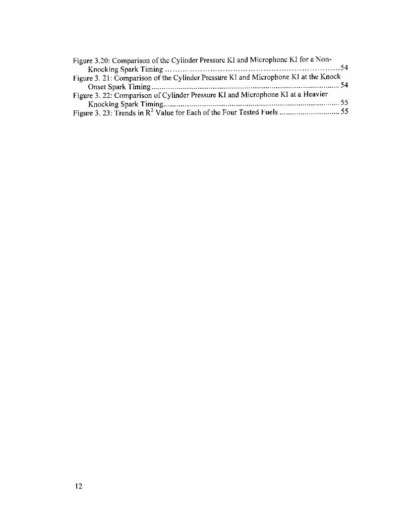
Figure 3.20: Comparison of the Cylinder Pressure KI and Microphone KI for a Non-

Knocking Spark Tim ing .................................................................. 54Figure 3. 21: Comparison of the Cylinder Pressure KI and Microphone KI at the Knock

O nset Spark T im ing ...................................................................................... ......... 54Figure 3. 22: Comparison of Cylinder Pressure KI and Microphone KI at a Heavier

K nocking Spark T im ing........................................................................................ 55Figure 3. 23: Trends in R2 Value for Each of the Four Tested Fuels ........................... 55

12

CHAPTER 1: INTRODUCTION

1.1 KNOCK FUNDAMENTALSKnock is a highly researched area because it is not adequately understood. Many also

believe knock to be a significant barrier to greatly improving the performance of spark-

ignited gasoline engines through turbocharging. Turbocharging forces more air into the

cylinder. This increase in air density causes a turbocharged engine to produce higher

brake mean effective pressures (BMEP) without greatly increasing the engine friction.

This means that an engine can be downsized while still meeting the same torque

requirements and increasing its part load efficiency. This path of turbocharging and

downsizing is similar to what has previously been done with diesel engines. The

challenge in turbocharging gasoline engines is the increased knock severity. Engine

knock is an unacceptable combustion phenomenon for the following two reasons: the

sound is unpleasant and undesirable to the passengers in a vehicle, and at a high enough

intensity, knock can lead to engine damage.

1.1.1 Knock Definition

Engine knock is a knocking or pinging sound that can be heard outside an operating

engine. It is caused by the rapid autoignition of a portion of the in-cylinder charge that

generates a local pressure pulse creating pressure oscillations. These oscillation then

propagate across the cylinder in a manner which creates noise outside the engine.[1] This

autoignition is usually initiated from one or more hot-spots in the end gas, the unburned

mixture ahead of the flame front. Not all autoignition events will lead to knock.

Many methods for the detection of knock onset have been explored. A brief list includes

the use of processed cylinder pressures, accelerometers to detect engine vibrations,

optical detectors, spark plug ionization probes, heat transfer data, as well as microphones

and the ear alone. For this work, knock onset is defined as the instant at which a

knocking or pinging sound can be heard through a set of headphones attached to a

microphone in the test cell. This microphone/headphone setup will be explained in more

detail in Section 2.2.8.

13

1.1.2 Factors that Affect Engine Knock

The thermodynamic state of the end gas in the cylinder is greatly affected by cylinder

pressure. An increase in end gas pressure increases end gas temperature which in turn

increases reaction rates. Factors that affect cylinder pressure are inlet pressure, air-fuel

ratio, spark timing, compression ratio, engine speed, charge preparation, and combustion

chamber geometry. Factors that affect end gas temperature and composition are mixture

composition and initial temperature. Following is a brief description of each of these

factors:

* Inlet pressure: A higher inlet pressure forces a larger amount of air-fuel mixture

into the cylinder which increases cylinder pressure and increases engine torque

output.

* Air-fuel ratio: Variations in the amount of excess air or excess fuel in the

cylinder changes the combustion rates and the energy release which in turn affects

cylinder pressure and end gas temperatures.

* Spark timing: Earlier spark timing causes earlier combustion which results in

higher cylinder pressures because combustion takes place in a smaller volume.

Knock is more likely with an earlier spark timing because the maximum end gas

temperature is increased.

* Compression ratio: A higher compression ratio leaves a smaller volume available

for combustion which increases cylinder pressure and end gas temperatures.

* Engine speed: A slower engine speed means that each cycle lasts longer resulting

in an end gas at a higher pressure and temperature for a longer period of time

making an autoignition event more likely to occur.

* Charge preparation: The amount of turbulence, swirl, and tumble affects the

homogeneity of the mixture as well as the end gas location in the cylinder.

" Combustion chamber geometry: The general shape of the combustion chamber, as

well as spark plug location, affects the flame front area and the distance the flame

front must travel. A small flame front or large distance slows combustion

increasing the likelihood of an autoignition event.

* Mixture composition: The mixture composition, including air-fuel ratio and

residual fraction, affects the ratio of specific heats (y) as per Equation (1.1).

14

T - ,(1.1)

A higher y, which is caused by a higher air-fuel ratio or a lower residual fraction,

leads to higher compression temperatures. The type of fuel and fuel additives can

also have an effect.

* Initial temperature: A higher initial temperature leads to a higher compression

temperature as shown in Equation (1.1). Initial temperature can be affected by the

temperature of the inlet air, heat transfer, and the residual gas fraction and

temperature.

1.2 PREVIOUS WORKWhile extensive work has been done in the field of engine knock research, this section

reviews some of the research that is most relevant to the specific objectives outlined in

the next section. Varying definitions and descriptions of knock are also included.

1.2.1 Brief Overview of Knock Detection MethodsLee, et al. [2] affirmed that cylinder pressure data gives the most accurate information

regarding knock; however, they also confirmed that there is a great deal of disagreement

on how cylinder pressure data should be processed and used. One method of data

processing proposed by this team was to use three narrow bandpass filters for the first,

second, and third harmonic knock frequencies. It was mentioned that the results attained,

especially that of knock intensity, vary with engine operating conditions, sensor location,

and the fuel used. Some of their other suggestions included: using a piece of tubing that

is funnel shaped at the ends as a wave guide to pick up the pressure signals with a

microphone and also combining audible detection by the ear alone with observation of

the vibration signal.

Various measures were used by Kaneyasu, et al. [3] to determine knock onset. These

methods included the use of a piezoelectric accelerometer to detect engine vibrations. A

cylinder pressure sensor was used in conjunction with the engine vibration data. The

15

cylinder pressure data was bandpass filtered at the most representative resonant

frequency and integrated. Knock intensity was determined by monitoring the signal to

noise ratio of the spectra.

Chiriac, Radu, and Apostolescu [4] also used a signal to noise ratio approach for finding

the crank angle of knock onset but acknowledged in the paper that there were problems

with the use of this method. Instead, they used a plot of knock intensity versus spark

timing in order to determine the knock threshold.

1.2.2 Variation in Levels of Pressure Waves

It is not necessary for each individual cycle in an engine to be rapidly autoigniting in

order to consider the engine as a whole to be knocking. In fact, it may be possible to

achieve full engine knock, under certain circumstances such as when using fuels that

have lower octane numbers, with as few as 6% of the cycles rapidly autoigniting.

It is stated in a paper by Grandin, et al. [5] that only autoignition events that cause a fast

energy release that produce pressure gradients triggering pressure oscillations at natural

frequencies will lead to the noise that generates engine knock.

Bradley and Morley [6] concluded from their studies that the spatial gradient of

temperature around the hot spots in the cylinder is important. More specifically, it is the

ratio of the temperature gradient in the hot spot to the critical temperature gradient that is

important. The critical temperature gradient is defined at the instant when the

autoignition front travels at the acoustic speed into the unburned mixture. When this

ratio is within a certain range, the major heat release is in the form of an acoustic wave,

and this wave may or may not reinforce the chemical wave. The act of these waves

reinforcing or canceling each other may differentiate between a knocking and non-

knocking individual cycle.

Konig and Sheppard [7] stated a similar proposal in an earlier paper. They state that

autoignition occurring late in a cycle does not lead to rapid pressure oscillations but

rather acts more like an extension of the main flame. They define autoignition as a

16

chemical reaction which accelerates to spontaneous, light-emitting ignition and knock as

abnormal oscillations in the cylinder pressure during combustion. They also

characterized knock by carbon formation and high velocity post-knock gas motions.

1.2.3 Proposed Mechanisms for the Increase in Pressure Oscillation AmplitudePan and Sheppard [8] maintain that rather than a single hot spot causing engine knock,

multiple hot spots are required. They found that pressure emanating from the first hot

spot will modify the temperature gradient around adjacent hot spots. This can lead to the

displacement of a second hot spot at a lower temperature by the expansion of the first hot

spot. The second hot spot may initially react more slowly than the first but can exhibit a

more violent reaction of the developing detonation type which leads to engine knock.

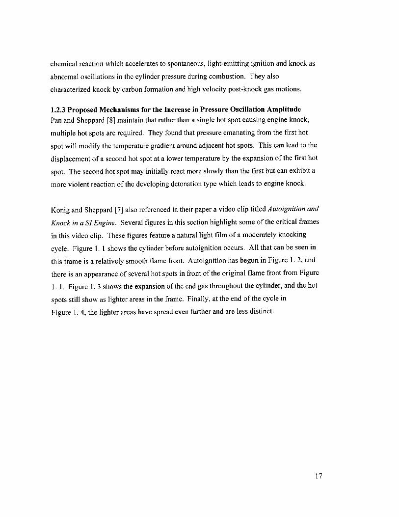
Konig and Sheppard [7] also referenced in their paper a video clip titled Autoignition and

Knock in a SI Engine. Several figures in this section highlight some of the critical frames

in this video clip. These figures feature a natural light film of a moderately knocking

cycle. Figure 1. 1 shows the cylinder before autoignition occurs. All that can be seen in

this frame is a relatively smooth flame front. Autoignition has begun in Figure 1. 2, and

there is an appearance of several hot spots in front of the original flame front from Figure

1. 1. Figure 1. 3 shows the expansion of the end gas throughout the cylinder, and the hot

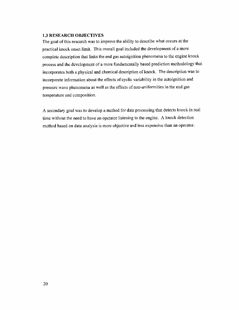
spots still show as lighter areas in the frame. Finally, at the end of the cycle in

Figure 1. 4, the lighter areas have spread even further and are less distinct.

17

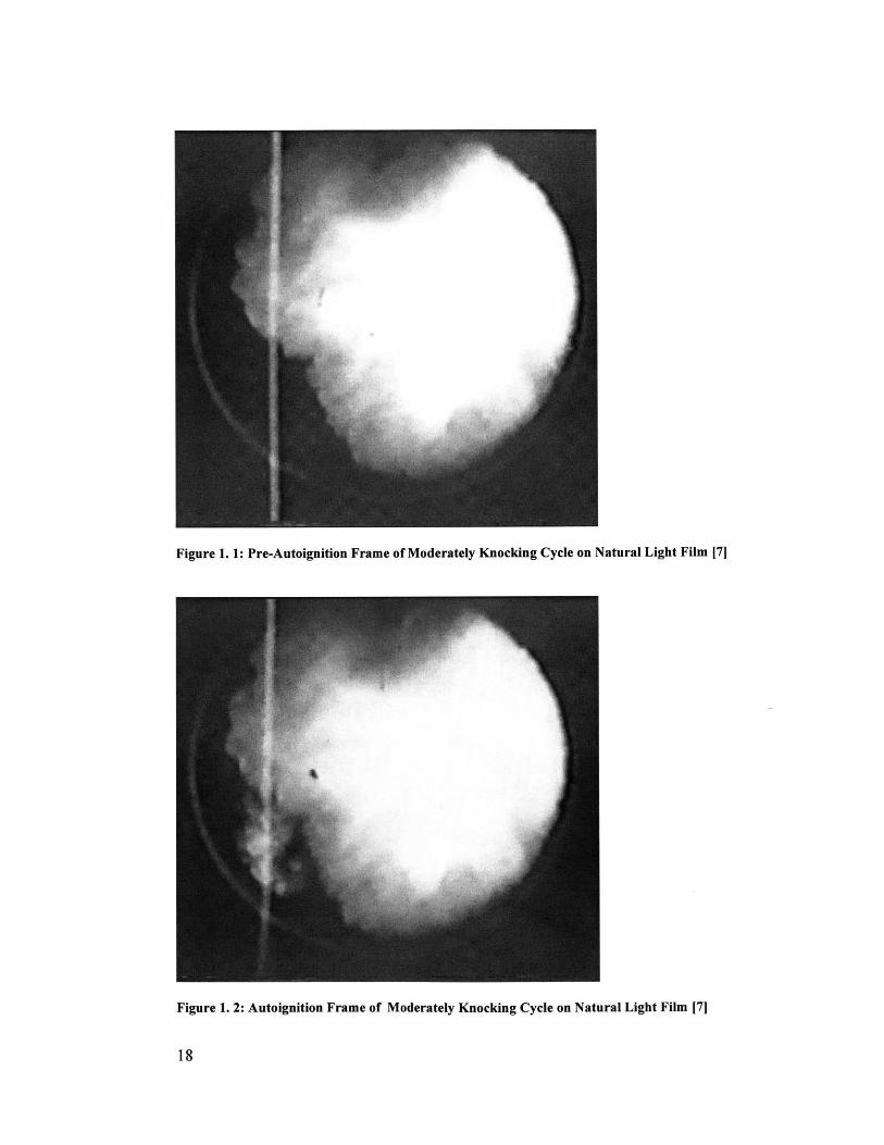
Figure 1. 1: Pre-Autoignition Frame of Moderately Knocking Cycle on Natural Light Film [7]

Figure 1. 2: Autoignition Frame of Moderately Knocking Cycle on Natural Light Film [7]

18

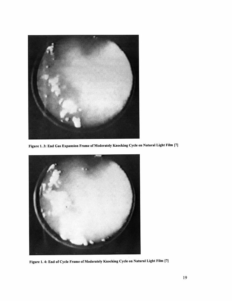
Figure 1. 3: End Gas Expansion Frame of Moderately Knocking Cycle on Natural Light Film [7]

Figure 1. 4: End of Cycle Frame of Moderately Knocking Cycle on Natural Light Film [71

19

1.3 RESEARCH OBJECTIVES

The goal of this research was to improve the ability to describe what occurs at the

practical knock onset limit. This overall goal included the development of a more

complete description that links the end gas autoignition phenomena to the engine knock

process and the development of a more fundamentally based prediction methodology that

incorporates both a physical and chemical description of knock. The description was to

incorporate information about the effects of cyclic variability in the autoignition and

pressure wave phenomena as well as the effects of non-uniformities in the end gas

temperature and composition.

A secondary goal was to develop a method for data processing that detects knock in real

time without the need to have an operator listening to the engine. A knock detection

method based on data analysis is more objective and less expensive than an operator.

20

CHAPTER 2: EXPERIMENTAL METHOD

2.1 TEST CELL SETUP

The test cell consists of a single-cylinder test engine, a variable frequency dynamometer,

and various pieces of control and test equipment.

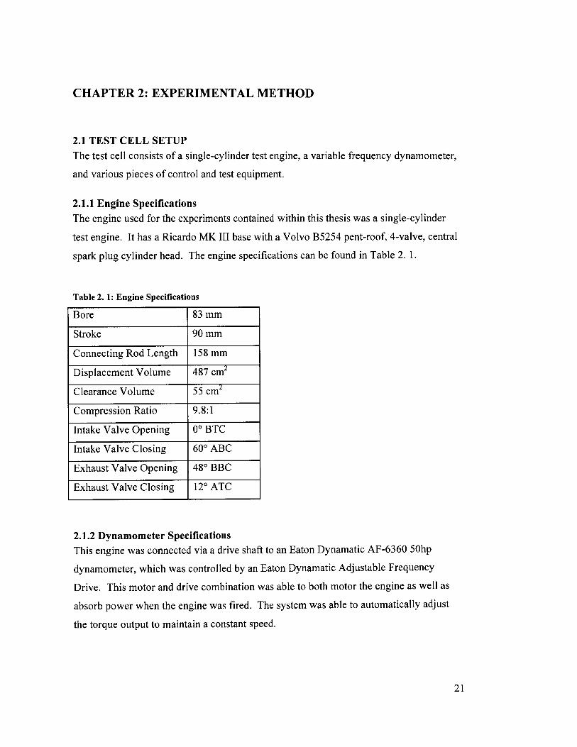
2.1.1 Engine Specifications

The engine used for the experiments contained within this thesis was a single-cylinder

test engine. It has a Ricardo MK III base with a Volvo B5254 pent-roof, 4-valve, central

spark plug cylinder head. The engine specifications can be found in Table 2. 1.

Table 2. 1: Engine Specifications

Bore 83 mm

Stroke 90 mm

Connecting Rod Length 158 mm

Displacement Volume 487 cm 2

Clearance Volume 55 cm2

Compression Ratio 9.8:1

Intake Valve Opening 00 BTC

Intake Valve Closing 600 ABC

Exhaust Valve Opening 480 BBC

Exhaust Valve Closing 120 ATC

2.1.2 Dynamometer Specifications

This engine was connected via a drive shaft to an Eaton Dynamatic AF-6360 50hp

dynamometer, which was controlled by an Eaton Dynamatic Adjustable Frequency

Drive. This motor and drive combination was able to both motor the engine as well as

absorb power when the engine was fired. The system was able to automatically adjust

the torque output to maintain a constant speed.

21

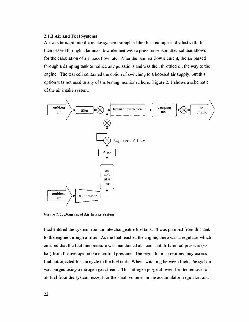
2.1.3 Air and Fuel Systems

Air was brought into the intake system through a filter located high in the test cell. It

then passed through a laminar flow element with a pressure sensor attached that allows

for the calculation of air mass flow rate. After the laminar flow element, the air passed

through a damping tank to reduce any pulsations and was then throttled on the way to the

engine. The test cell contained the option of switching to a boosted air supply, but this

option was not used in any of the testing mentioned here. Figure 2. 1 shows a schematic

of the air intake system.

ambient fitrlamninar flow element damping to n

Regulator to 0-1 bar

filter

rairtankat 4bar

ambient

Figure 2. 1: Diagram of Air Intake System

Fuel entered the system from an interchangeable fuel tank. It was pumped from this tank

to the engine through a filter. As the fuel reached the engine, there was a regulator which

ensured that the fuel line pressure was maintained at a constant differential pressure (-3

bar) from the average intake manifold pressure. The regulator also returned any excess

fuel not injected for the cycle to the fuel tank. When switching between fuels, the system

was purged using a nitrogen gas stream. This nitrogen purge allowed for the removal of

all fuel from the system, except for the small volumes in the accumulator, regulator, and

22

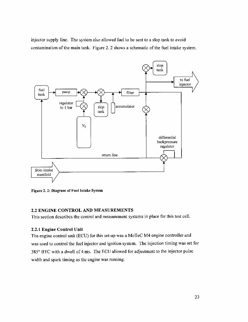
injector supply line. The system also allowed fuel to be sent to a slop tank to avoid

contamination of the main tank. Figure 2. 2 shows a schematic of the fuel intake system.

sloptank

tan PUMP filter A

regulatorto I bar slop acuutr

tank

N2

dba

return line

to fuelinjector

ifferentialckpressureregulator

from intakemanifold

Figure 2. 2: Diagram of Fuel Intake System

2.2 ENGINE CONTROL AND MEASUREMENTS

This section describes the control and measurement systems in place for this test cell.

2.2.1 Engine Control Unit

The engine control unit (ECU) for this set-up was a MoTeC M4 engine controller and

was used to control the fuel injector and ignition system. The injection timing was set for

3850 BTC with a dwell of 4 ms. The ECU allowed for adjustment to the injector pulse

width and spark timing as the engine was running.

23

2.2.2 Intake Pressure Control and Measurement

The manifold pressure was controlled by manually adjusting a throttle valve from outside

the test cell through the use of a stepper motor. Pressure transducers measuring absolute

pressure were used to measure intake pressure at two locations. The first location, which

measured the pressure of the air damping tank, was between the air flow meter and the

throttle plate. The second location, which was used to measure manifold absolute

pressure (MAP), was between the throttle plate and the engine. Both measurements had

digital readouts to display the results.

2.2.3 Temperature Control and Measurement

The temperatures of engine coolant and engine oil were controlled. The engine coolant

temperature was maintained between 90 'C and 95 'C by an electric heater/electronic

thermostat and cold water heat exchanger/mechanical thermostat combination. The oil

temperature was maintained between 70 'C and 80 'C by an electric heater/electronic

thermostat. The engine had four temperature measurement locations including the engine

coolant inlet, the intake air in the tank between the flow meter and the throttle plate, the

engine oil inlet, and the engine exhaust approximately 2 cm from the exhaust port outlet.

2.2.4 Air Flow Measurement

The volumetric flow rate of air was determined with the use of a differential pressure

sensor across a laminar flow element. The volumetric flow rate was then converted to a

mass flow rate using the ideal gas law as well as the air tank pressure and temperature

measurements. A humidity measurement was used to correct the air mass flow rate for

water content. The accuracy of the air mass flow rate was approximately 2%.

2.2.5 Fuel Flow Measurement

The fuel injector pulse width was used for determining the amount of fuel injected during

each cycle. This method allows for fast measurements with an accuracy of roughly 2%.

As mentioned earlier, the fuel pressure regulator maintains a constant differential

between the average intake manifold pressure and the fuel injector supply line pressure.

When the injector is open there is a constant flow through the injector orifice. Using a

previously completed experimental calibration, the injector pulse width can be used to

calculate the mass of injected fuel. The limitations in accuracy for this method are due to

24

pressure variations across the injector caused by high-speed fluctuations in the intake

manifold pressure as well as effects caused by variations in fuel density caused by

temperature variations.

2.2.6 Air-Fuel Ratio MeasurementA Universal Exhaust Gas Oxygen (UEGO) sensor was used to measure exhaust gas

oxygen content. The UEGO reading was then converted to an air-fuel equivalence ratio

or lambda reading with the use of a Horiba Mexa- 11 O analyzer.

2.2.7 Cylinder Pressure MeasurementCylinder pressure was measured using a Kistler 6125A piezoelectric pressure transducer

with a flame arrestor. The current signal from this pressure transducer was converted to a

voltage signal with the use of a charge amplifier. This voltage signal was then collected

at a rate of approximately ten times per crank angle degree using a National Instruments

6023E data acquisition card triggered by a BEI crankshaft encoder. A program written in

National Instruments LabVIEW recorded 100 cycles of cylinder pressure data when

triggered.

This cylinder pressure data in combination with a version of Sloan Automotive

Laboratory's burn rate analysis software, modified for use with high acquisition speed

data, was used to calculate:

* Peak pressure

* Crank angle of peak pressure

* 0-10% mass fraction burned time



* Net Indicated Mean Effective Pressure (NIMEP)

2.2.8 Knock DetectionA microphoned audible knock method was used to detect knock onset. A microphone

hung ~1/4 inch above the valve cover of the engine. This microphone was connected to

an equalizer set to remove all frequencies except those near 6 kHz and 12 kHz. The

25

audio signal was then passed to a set of headphones where the operator could listen to the

signal in order to detect knocking conditions.

This knock detection method was chosen because it was shown effective in previous

work [9] and because it avoided the complexity of a sensor-based knock detection

system. It can be roughly estimated that microphone knock occurs at a spark timing 2

crank angle degrees more retarded than knock that can be detected by the naked ear. This

method is somewhat subjective, but on average, between two different operators, the

knock limit is agreed upon within two octane numbers or 2 crank angle degrees.

2.2.9 Microphone MeasurementThe National Instruments LabVIEW software was also set up to record the signal heard

by the microphone. One hundred cycles of the microphone signal could be recorded

simultaneously with the cylinder pressure data.

2.3 EXPERIMENTAL PROCEDURES AND INFORMATION

Tests were completed to collect data that could be analyzed in order to gain a better

understand the knock onset phenomena.

2.3.1 Experimental Procedure

Before beginning any experiments, both the dynamometer and engine were fully warmed

up. Below is a list of the steps taken in order to complete a spark timing sweep.

Experimental results were recorded in a spreadsheet which was used to calculate burn

angles and other relevant parameters.

1. Set the engine speed with the dynamometer controller.

2. Position the throttle plate to the wide-open position.

3. Make an initial estimate of the maximum brake torque (MBT) timing from

previous trends.

4. Adjust the fuel injector pulse width using the MoTeC ECU until a stoichiometric

air-fuel ratio is achieved.

5. Using the microphone and headphones, find the spark timing at which knock

onset occurs. Advance the spark timing by 3' CA.

26

6. Record operating conditions and cylinder pressure data.

7. Retard the spark timing in increments of 1* CA, repeating Step 6 for each

increment until the spark timing is 3* CA more retarded than the knock onset

timing. While retarding the spark timing, minor adjustments to the throttle

position may need to be made in order to maintain a stoichiometric exhaust air-

fuel ratio. Care should be taken to avoid exceeding the maximum cylinder

pressure of 110 bar, an exhaust temperature greater than 750* C, or any extreme

knocking condition that might lead to engine damage.

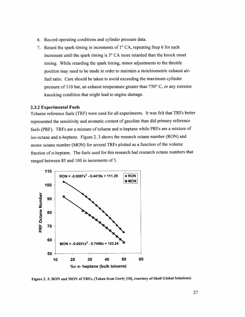
2.3.2 Experimental Fuels

Toluene reference fuels (TRF) were used for all experiments. It was felt that TRFs better

represented the sensitivity and aromatic content of gasoline than did primary reference

fuels (PRF). TRFs are a mixture of toluene and n-heptane while PRFs are a mixture of

iso-octane and n-heptane. Figure 2. 3 shows the research octane number (RON) and

motor octane number (MON) for several TRFs plotted as a function of the volume

fraction of n-heptane. The fuels used for this research had research octane numbers that

ranged between 85 and 100 in increments of 5.

110 -RON = -0.0097x 2 - 0.4419x + 111.29 + RON

E MON100 -

90 -Ez0c 80

0u700.

60MON = -0.0031x2 - 0.7498x + 103.24

5010 20 30 40 50 60

%v n- heptane (bulk toluene)

Figure 2. 3: RON and MON of TRFs, (Taken from Gerty [101, courtesy of Shell Global Solutions)

27


28

CHAPTER 3: DATA AND DATA PROCESSING METHODS

3.1 DATA SETSAll cylinder pressure and microphone data were acquired at a high acquisition speed of

90 kHz, which at an engine speed of 1500 RPM is equivalent to 10 samples per crank

angle degree. Data acquisition was triggered for every cycle by the BDC signal.

Previously, most cylinder pressure data had been obtained using a lower sampling

frequency of only 1 sample per crank angle degree. It was determined, however, that this

slower sampling rate did not allow for an adequate observation of the more subtle

behaviors of the cylinder pressure during conditions of engine knock.

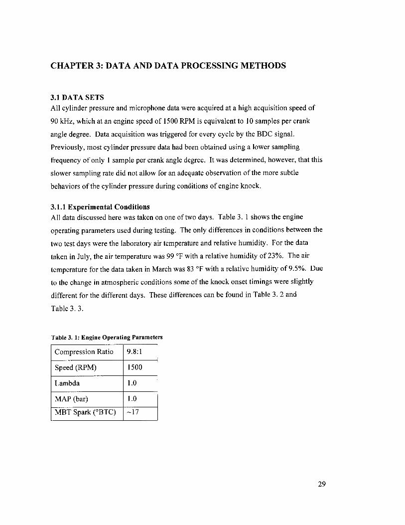
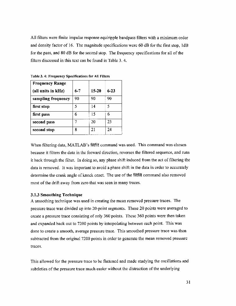
3.1.1 Experimental ConditionsAll data discussed here was taken on one of two days. Table 3. 1 shows the engine

operating parameters used during testing. The only differences in conditions between the

two test days were the laboratory air temperature and relative humidity. For the data

taken in July, the air temperature was 99 'F with a relative humidity of 23%. The air

temperature for the data taken in March was 83 'F with a relative humidity of 9.5%. Due

to the change in atmospheric conditions some of the knock onset timings were slightly

different for the different days. These differences can be found in Table 3. 2 and

Table 3. 3.

Table 3. 1: Engine Operating Parameters

Compression Ratio 9.8:1

Speed (RPM) 1500

Lambda 1.0

MAP (bar) 1.0

MBT Spark (*BTC) ~17

29

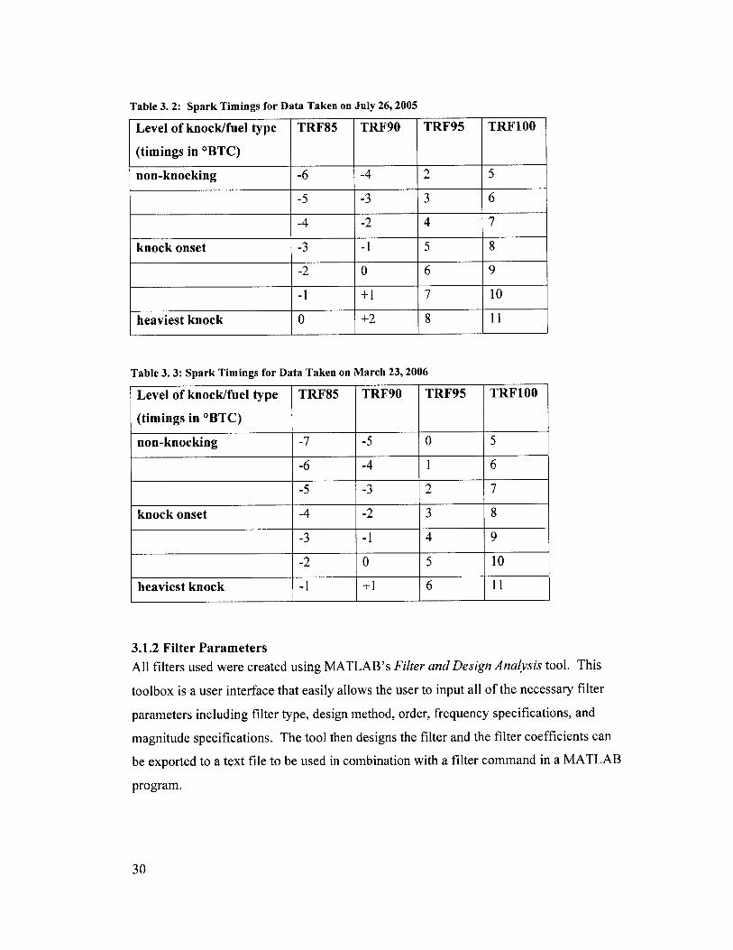
Table 3. 2: Spark Timings for Data Taken on July 26, 2005

Level of knock/fuel type TRF85 TRF90 TRF95 TRF100

(timings in OBTC)

non-knocking -6 -4 2 5

-5 -3 3 6

-4 -2 4 7

knock onset -3 -1 5 8

-2 0 6 9

-1 +1 7 10

heaviest knock 0 +2 8 11

Table 3. 3: Spark Timings for Data Taken on March 23, 2006

Level of knock/fuel type TRF85 TRF90 TRF95 TRF100

(timings in OBTC)

non-knocking -7 -5 0 5

-6 -4 1 6

-5 -3 2 7

knock onset -4 -2 3 8

-3 -1 4 9

-2 0 5 10

heaviest knock -1 +1 6 11

3.1.2 Filter Parameters

All filters used were created using MATLAB's Filter and Design Analysis tool. This

toolbox is a user interface that easily allows the user to input all of the necessary filter

parameters including filter type, design method, order, frequency specifications, and

magnitude specifications. The tool then designs the filter and the filter coefficients can

be exported to a text file to be used in combination with a filter command in a MATLAB

program.

30

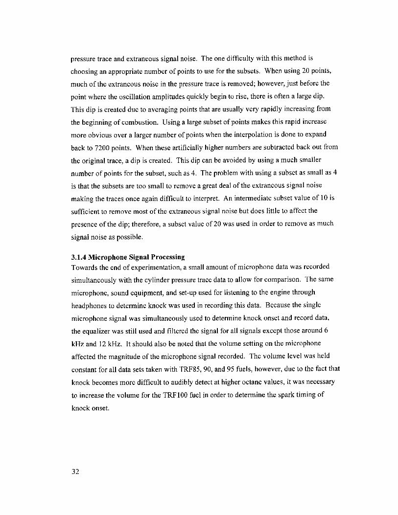
All filters were finite impulse response equiripple bandpass filters with a minimum order

and density factor of 16. The magnitude specifications were 60 dB for the first stop, 1dB

for the pass, and 80 dB for the second stop. The frequency specifications for all of the

filters discussed in this text can be found in Table 3. 4.

Table 3. 4: Frequency Specifications for All Filters

Frequency Range

(all units in kHz) 6-7 15-20 6-23

sampling frequency 90 90 90

first stop 5 14 5

first pass 6 15 6

second pass 7 20 23

second stop 8 21 24

When filtering data, MATLAB's filtfilt command was used. This command was chosen

because it filters the data in the forward direction, reverses the filtered sequence, and runs

it back through the filter. In doing so, any phase shift induced from the act of filtering the

data is removed. It was important to avoid a phase shift in the data in order to accurately

determine the crank angle of knock onset. The use of the filtfilt command also removed

most of the drift away from zero that was seen in many traces.

3.1.3 Smoothing TechniqueA smoothing technique was used in creating the mean removed pressure traces. The

pressure trace was divided up into 20-point segments. These 20 points were averaged to

create a pressure trace consisting of only 360 points. These 360 points were then taken

and expanded back out to 7200 points by interpolating between each point. This was

done to create a smooth, average pressure trace. This smoothed pressure trace was then

subtracted from the original 7200 points in order to generate the mean removed pressure

traces.

This allowed for the pressure trace to be flattened and made studying the oscillations and

subtleties of the pressure trace much easier without the distraction of the underlying

31

pressure trace and extraneous signal noise. The one difficulty with this method is

choosing an appropriate number of points to use for the subsets. When using 20 points,

much of the extraneous noise in the pressure trace is removed; however, just before the

point where the oscillation amplitudes quickly begin to rise, there is often a large dip.

This dip is created due to averaging points that are usually very rapidly increasing from

the beginning of combustion. Using a large subset of points makes this rapid increase

more obvious over a larger number of points when the interpolation is done to expand

back to 7200 points. When these artificially higher numbers are subtracted back out from

the original trace, a dip is created. This dip can be avoided by using a much smaller

number of points for the subset, such as 4. The problem with using a subset as small as 4

is that the subsets are too small to remove a great deal of the extraneous signal noise

making the traces once again difficult to interpret. An intermediate subset value of 10 is

sufficient to remove most of the extraneous signal noise but does little to affect the

presence of the dip; therefore, a subset value of 20 was used in order to remove as much

signal noise as possible.

3.1.4 Microphone Signal ProcessingTowards the end of experimentation, a small amount of microphone data was recorded

simultaneously with the cylinder pressure trace data to allow for comparison. The same

microphone, sound equipment, and set-up used for listening to the engine through

headphones to determine knock was used in recording this data. Because the single

microphone signal was simultaneously used to determine knock onset and record data,

the equalizer was still used and filtered the signal for all signals except those around 6

kHz and 12 kHz. It should also be noted that the volume setting on the microphone

affected the magnitude of the microphone signal recorded. The volume level was held

constant for all data sets taken with TRF85, 90, and 95 fuels, however, due to the fact that

knock becomes more difficult to audibly detect at higher octane values, it was necessary

to increase the volume for the TRF 100 fuel in order to determine the spark timing of

knock onset.

32

3.2 DATA PROCESSING AND ANALYZATIONThis section contains a summary of the successful data processing and analysis methods

found throughout this research.

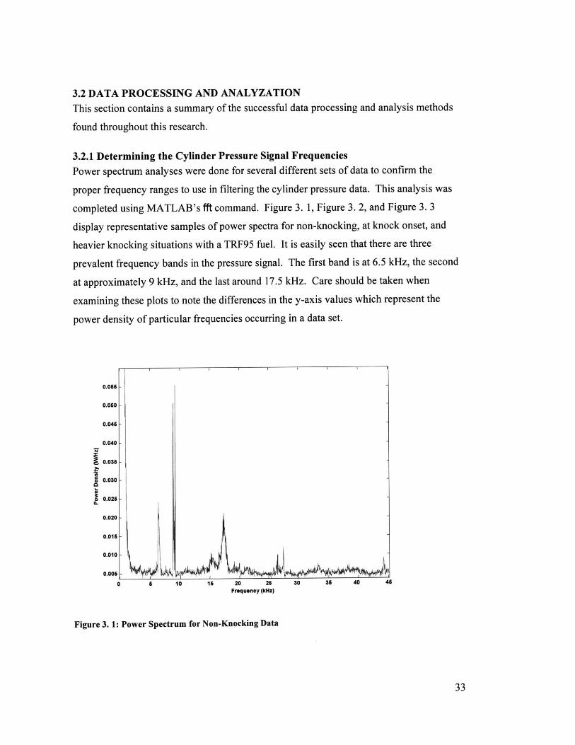
3.2.1 Determining the Cylinder Pressure Signal Frequencies

Power spectrum analyses were done for several different sets of data to confirm the

proper frequency ranges to use in filtering the cylinder pressure data. This analysis was

completed using MATLAB's fft command. Figure 3. 1, Figure 3. 2, and Figure 3. 3

display representative samples of power spectra for non-knocking, at knock onset, and

heavier knocking situations with a TRF95 fuel. It is easily seen that there are three

prevalent frequency bands in the pressure signal. The first band is at 6.5 kHz, the second

at approximately 9 kHz, and the last around 17.5 kHz. Care should be taken when

examining these plots to note the differences in the y-axis values which represent the

power density of particular frequencies occurring in a data set.

5 10 16 20 26Frequency (kHz)

30 36 40 45

Figure 3. 1: Power Spectrum for Non-Knocking Data

33

0.066

0.060

IF~

CL

0.046 -

0.040 -

0.036 -

0.030 -

0.026 -

0.020 -

0.015 -IJL0.010

0.0051-0

I

0.30f '

0.25

0.20

0.15

0.10

0.05

SI

5 10 15 20 25

Frequency (kHz)

30 35 40

Figure 3. 2: Power Spectrum for Knock Onset Data

5 10 15 20 25

Frequency (kHz)

30 35 40 45

Figure 3. 3: Power Spectrum for Heavy Knocking Data

34

(A

0a0

0

0

I(0

Sa0

00.

2.0

1.8

1.6

1.4

1.2

1.0

0.8

0.6

0.4

0.2

0.0

- Ii

II

) 1k\2~ \/\

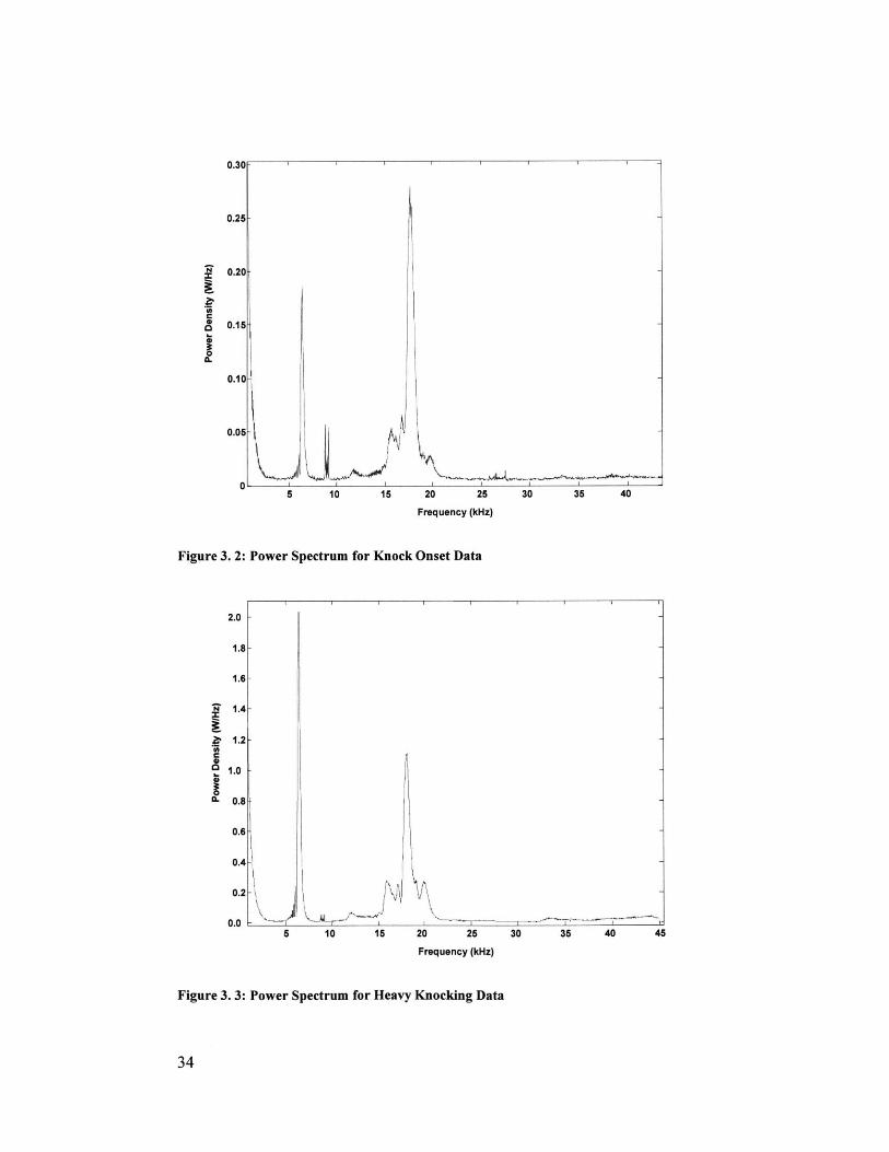
For data sets that are non-knocking (Figure 3. 1), the second band shows the most

prevalence, with the first and third showing considerably smaller power densities.

Progressing to the knock onset power spectrum (Figure 3. 2), the power density of the

second band maintains the same numeric power density value, but there is a dramatic

increase in the power density for both the first and third bands. A nearly ten-fold

increase in the first band and an over ten-fold increase in the third band are observed. It

is not always the case, that the third band shows a greater prominence than the first.

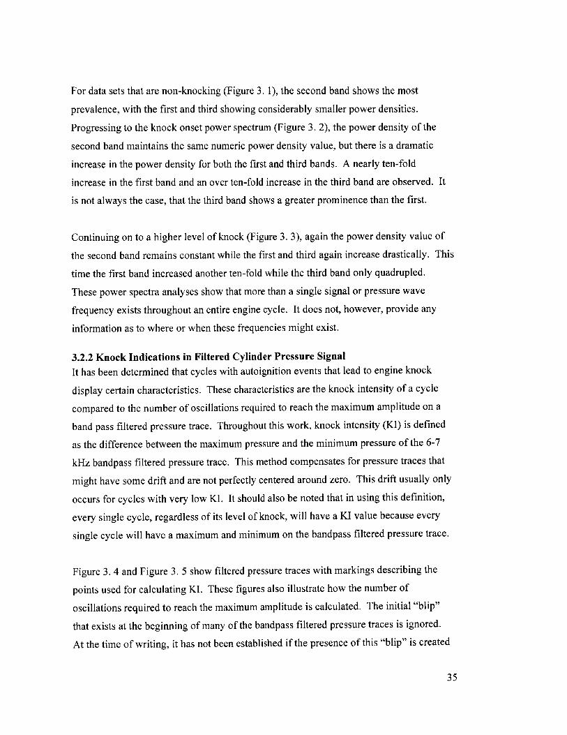
Continuing on to a higher level of knock (Figure 3. 3), again the power density value of

the second band remains constant while the first and third again increase drastically. This

time the first band increased another ten-fold while the third band only quadrupled.

These power spectra analyses show that more than a single signal or pressure wave

frequency exists throughout an entire engine cycle. It does not, however, provide any

information as to where or when these frequencies might exist.

3.2.2 Knock Indications in Filtered Cylinder Pressure SignalIt has been determined that cycles with autoignition events that lead to engine knock

display certain characteristics. These characteristics are the knock intensity of a cycle

compared to the number of oscillations required to reach the maximum amplitude on a

band pass filtered pressure trace. Throughout this work, knock intensity (KI) is defined

as the difference between the maximum pressure and the minimum pressure of the 6-7

kHz bandpass filtered pressure trace. This method compensates for pressure traces that

might have some drift and are not perfectly centered around zero. This drift usually only

occurs for cycles with very low KI. It should also be noted that in using this definition,

every single cycle, regardless of its level of knock, will have a KI value because every

single cycle will have a maximum and minimum on the bandpass filtered pressure trace.

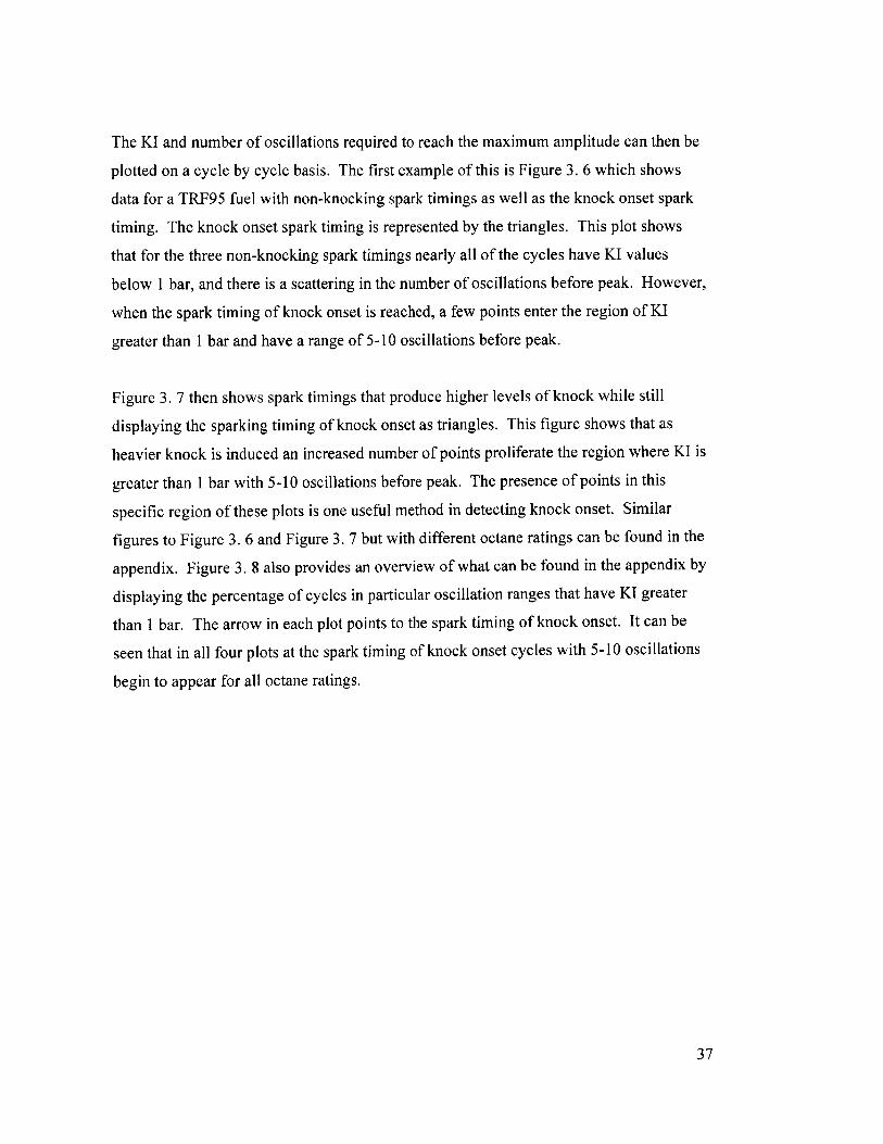
Figure 3. 4 and Figure 3. 5 show filtered pressure traces with markings describing the

points used for calculating KI. These figures also illustrate how the number of

oscillations required to reach the maximum amplitude is calculated. The initial "blip"

that exists at the beginning of many of the bandpass filtered pressure traces is ignored.

At the time of writing, it has not been established if the presence of this "blip" is created

35

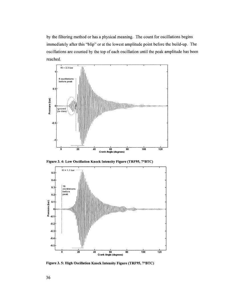
by the filtering method or has a physical meaning. The count for oscillations begins

immediately after this "blip" or at the lowest amplitude point before the build-up. The

oscillations are counted by the top of each oscillation until the peak amplitude has been

reached.

K1= 2.3

5 osctathbefore p

(to date)

bar

ns

MA

20 40 60Crank Angle (degrees)

0 100 120

Figure 3. 4: Low Oscillation Knock Intensity Figure (TRF95, 7 0BTC)

0 20 40 60Crank Angle (degrees)

80 100 120

Figure 3. 5: High Oscillation Knock Intensity Figure (TRF95, 70BTC)

36

I

0.5

0

-0.5

1

0

0.5

0.4

0.3

0.2

0.1

.010

.0.2

-0.3

-0.4

-015

KI = 1A bar

before

VW %A\wwwwvVWMA wvvWA-4wN

I ~

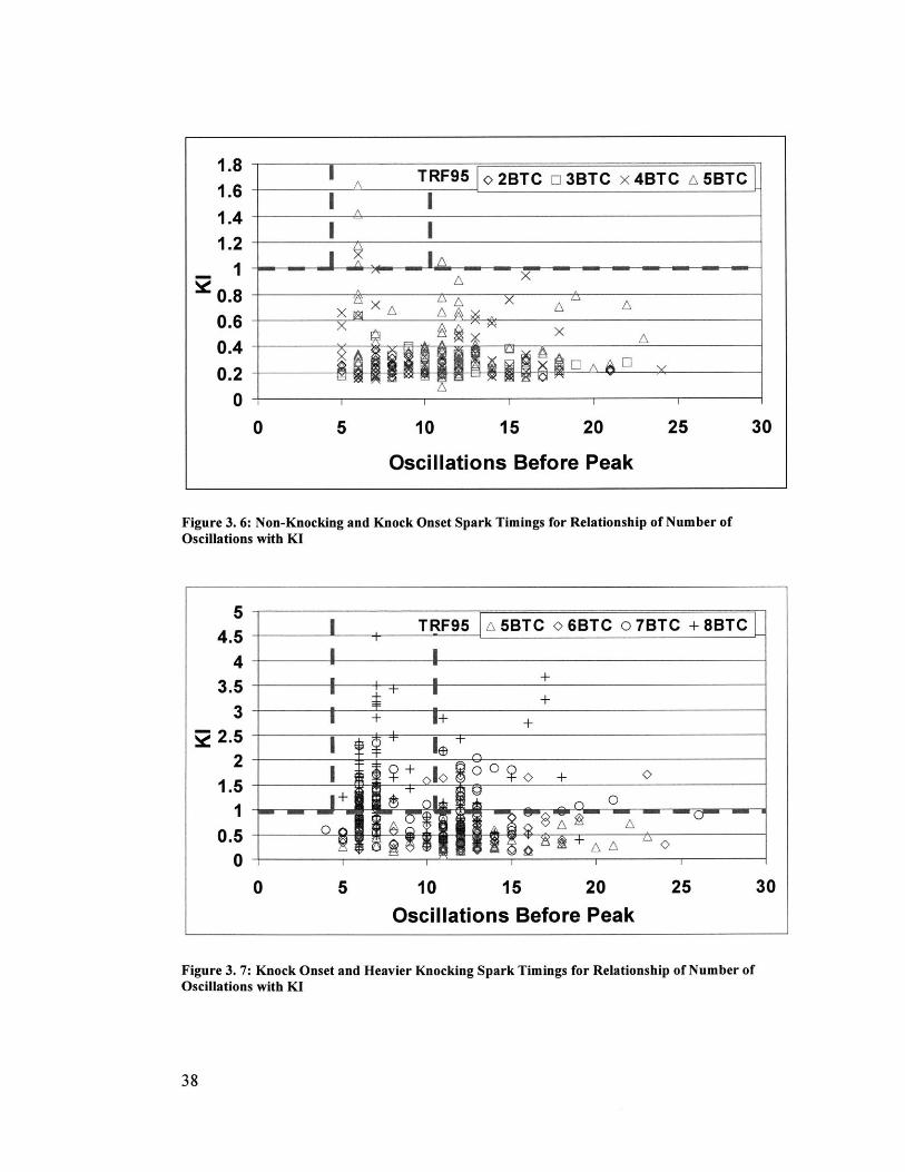
The KI and number of oscillations required to reach the maximum amplitude can then be

plotted on a cycle by cycle basis. The first example of this is Figure 3. 6 which shows

data for a TRF95 fuel with non-knocking spark timings as well as the knock onset spark

timing. The knock onset spark timing is represented by the triangles. This plot shows

that for the three non-knocking spark timings nearly all of the cycles have KI values

below 1 bar, and there is a scattering in the number of oscillations before peak. However,

when the spark timing of knock onset is reached, a few points enter the region of KI

greater than 1 bar and have a range of 5-10 oscillations before peak.

Figure 3. 7 then shows spark timings that produce higher levels of knock while still

displaying the sparking timing of knock onset as triangles. This figure shows that as

heavier knock is induced an increased number of points proliferate the region where KI is

greater than 1 bar with 5-10 oscillations before peak. The presence of points in this

specific region of these plots is one useful method in detecting knock onset. Similar

figures to Figure 3. 6 and Figure 3. 7 but with different octane ratings can be found in the

appendix. Figure 3. 8 also provides an overview of what can be found in the appendix by

displaying the percentage of cycles in particular oscillation ranges that have KI greater

than 1 bar. The arrow in each plot points to the spark timing of knock onset. It can be

seen that in all four plots at the spark timing of knock onset cycles with 5-10 oscillations

begin to appear for all octane ratings.

37

1.81.61.4

1.2

0.80.60.40.2

00 5 10 15 20 25 30

Oscillations Before Peak

Figure 3. 6: Non-Knocking and Knock Onset Spark Timings for Relationship of Number ofOscillations with KI

54.5 +T RF95 F_ 5BT C o 6BT C o 7BT C + 8BT C

43.5

0

22.5 + 1 +2

1.5 +1+

0.5-+

0 1

0 5 10 15 20 25 30


Figure 3. 7: Knock Onset and Heavier Knocking Spark Timings for Relationship of Number ofOscillations with KI

38

TRF95 1 2BTC E 3BTC x 4BTC A 5BTC

I IA

I Ax A X x x A

A A ^ A

I I I I

1 0 0 - - - - - - - - - - - - - - - .- - - - - - - - - -

TRF8S -+-5-10 oscIGations - >1 )0o scaUIs nsS0-

80

70

so-o60(A

o 40-

30-

20

10

4 -6 -4 -3 -2 -1 0spark timing

100 -1 TRF95 + 5-10 os0Cllains 4 :11osoflafons

iD 80

70

60

50

40

30

20

10

0 .. ... ~.~ .

2 3 4 6 6 7 8spark timing

100 -

90-

080

70C260

=50

040

030

:120 -

10

0:u

TRF90 * -10 oswiiianans -U->10 osolastron

"A4 -3 .2 -1

spak timing

0IM

0

0.2

80

70

80

10

0

0 1 2

.... ..... .. ..... .. ... ... ... ... ........... ..... .... ...... ......... .....-*. .... .... ...

5 6 7 8 9 10 11

Figure 3. 8: Trends in the Number of Oscillations for all Four Fuel Types

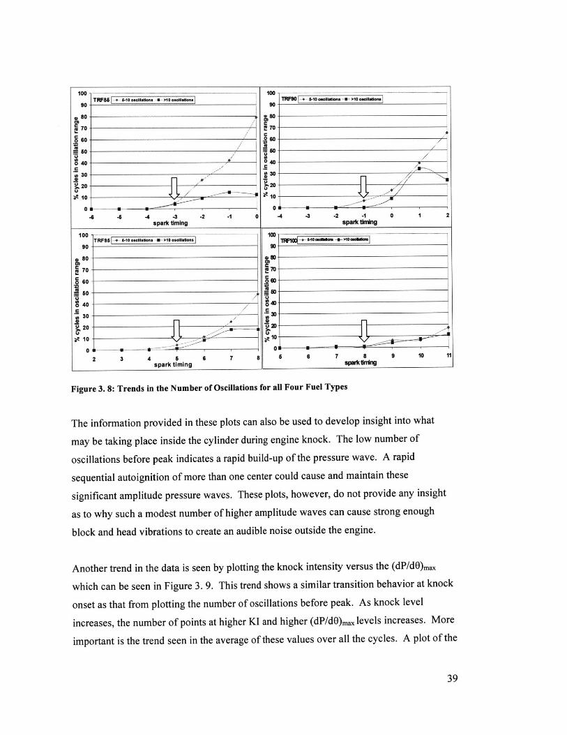
The information provided in these plots can also be used to develop insight into what

may be taking place inside the cylinder during engine knock. The low number of

oscillations before peak indicates a rapid build-up of the pressure wave. A rapid

sequential autoignition of more than one center could cause and maintain these

significant amplitude pressure waves. These plots, however, do not provide any insight

as to why such a modest number of higher amplitude waves can cause strong enough

block and head vibrations to create an audible noise outside the engine.

Another trend in the data is seen by plotting the knock intensity versus the (dP/d6)ma

which can be seen in Figure 3. 9. This trend shows a similar transition behavior at knock

onset as that from plotting the number of oscillations before peak. As knock level

increases, the number of points at higher KI and higher (dP/dO)ma levels increases. More

important is the trend seen in the average of these values over all the cycles. A plot of the

39

-.5j

.1

spark tinfng

-

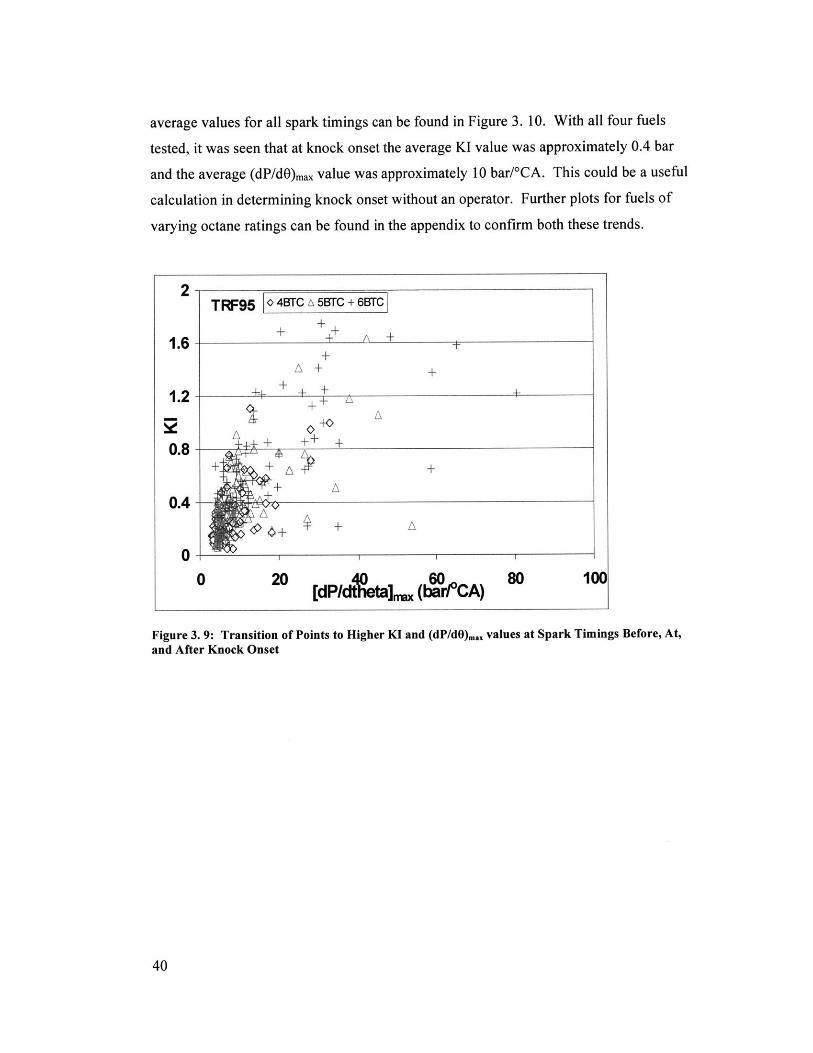
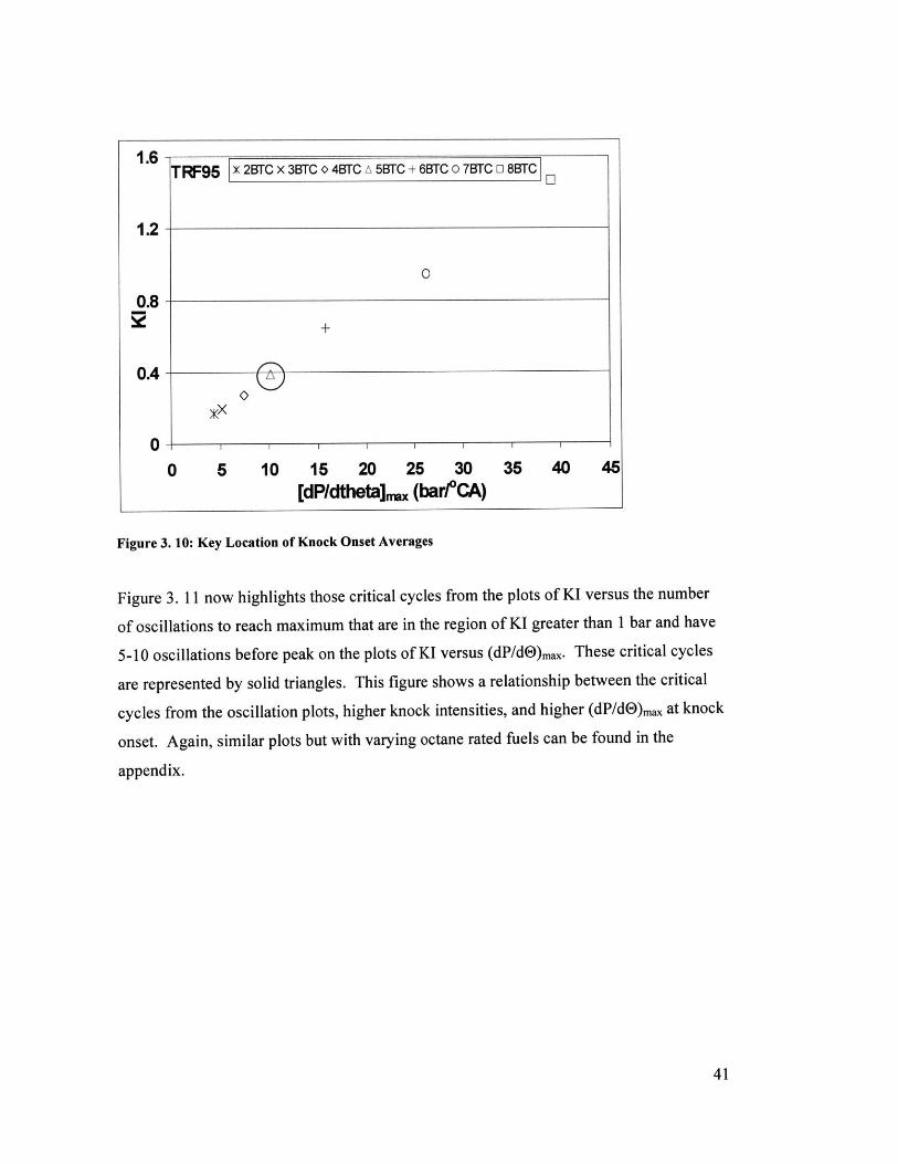
average values for all spark timings can be found in Figure 3. 10. With all four fuels

tested, it was seen that at knock onset the average KI value was approximately 0.4 bar

and the average (dP/dO)max value was approximately 10 bar/*CA. This could be a useful

calculation in determining knock onset without an operator. Further plots for fuels of

varying octane ratings can be found in the appendix to confirm both these trends.

2

1.6

1.2

0.8

0.4

0

0 20

TRF95 104BTCA 5BTC + 6BrC

++

+ + +

+ +

+ + + \ A

+ + + +

+ +A

++

4d 60[dP/dffietaJ3 (bar/ 0CA)

80 100

Spark Timings Before, At,

40

Figure 3. 9: Transition of Points to Higher KI and (dP/dO)max values atand After Knock Onset

1.6

1.2

0

0.8

0.4-

0 5 10 15 20 25 30 35 40 45[dPdtheta]rmx (bar/*CA)

Figure 3. 10: Key Location of Knock Onset Averages

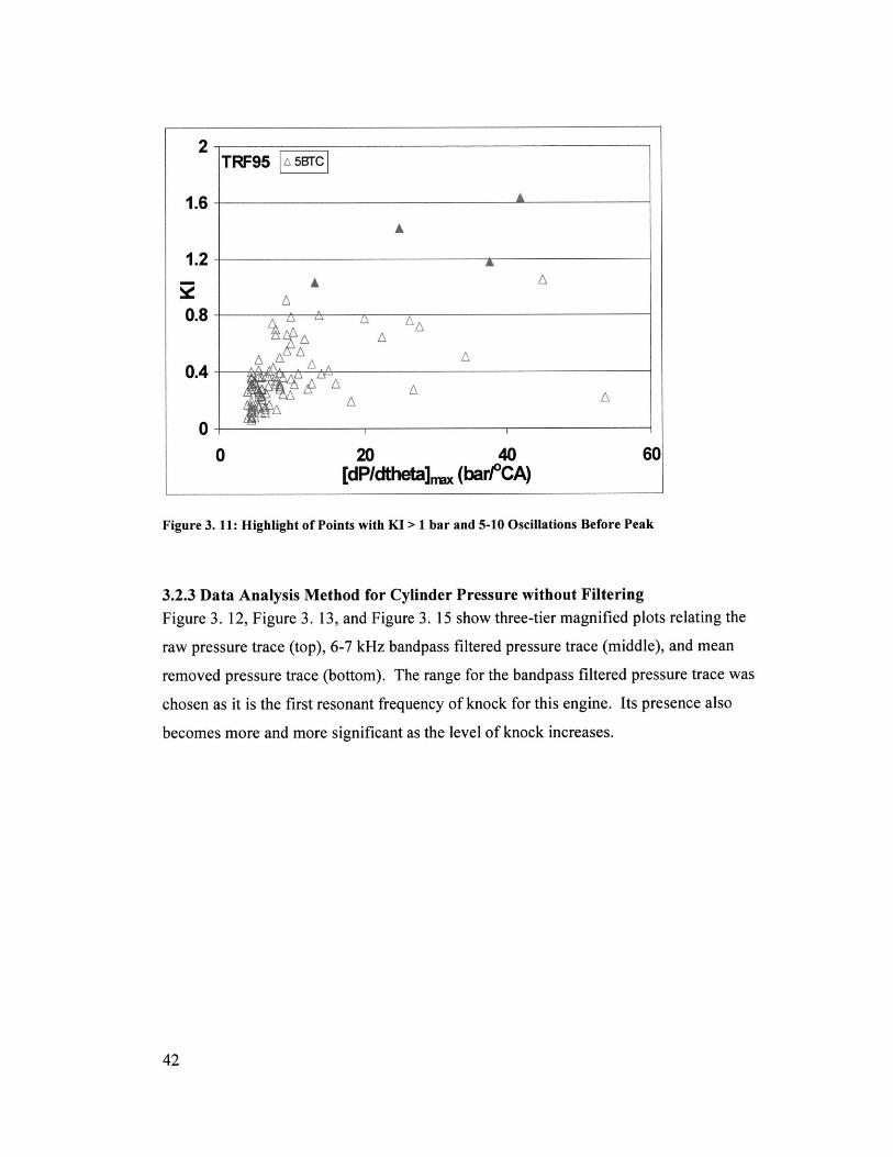
Figure 3. 11 now highlights those critical cycles from the plots of KI versus the number

of oscillations to reach maximum that are in the region of KI greater than 1 bar and have

5-10 oscillations before peak on the plots of KI versus (dP/dO)m.. These critical cycles

are represented by solid triangles. This figure shows a relationship between the critical

cycles from the oscillation plots, higher knock intensities, and higher (dP/d)ma at knock

onset. Again, similar plots but with varying octane rated fuels can be found in the

appendix.

41

TRF95 X 2ETC X 3BTC 0 4BTC A 51TC + 6BTC 0 7BTC 0 8BTC

2

1.6 A

A

1.2- A

A

0.8 L A

0. A

L_

00 20 40 60

[dP/dtheta]max (barf*CA)

Figure 3. 11: Highlight of Points with KI > 1 bar and 5-10 Oscillations Before Peak

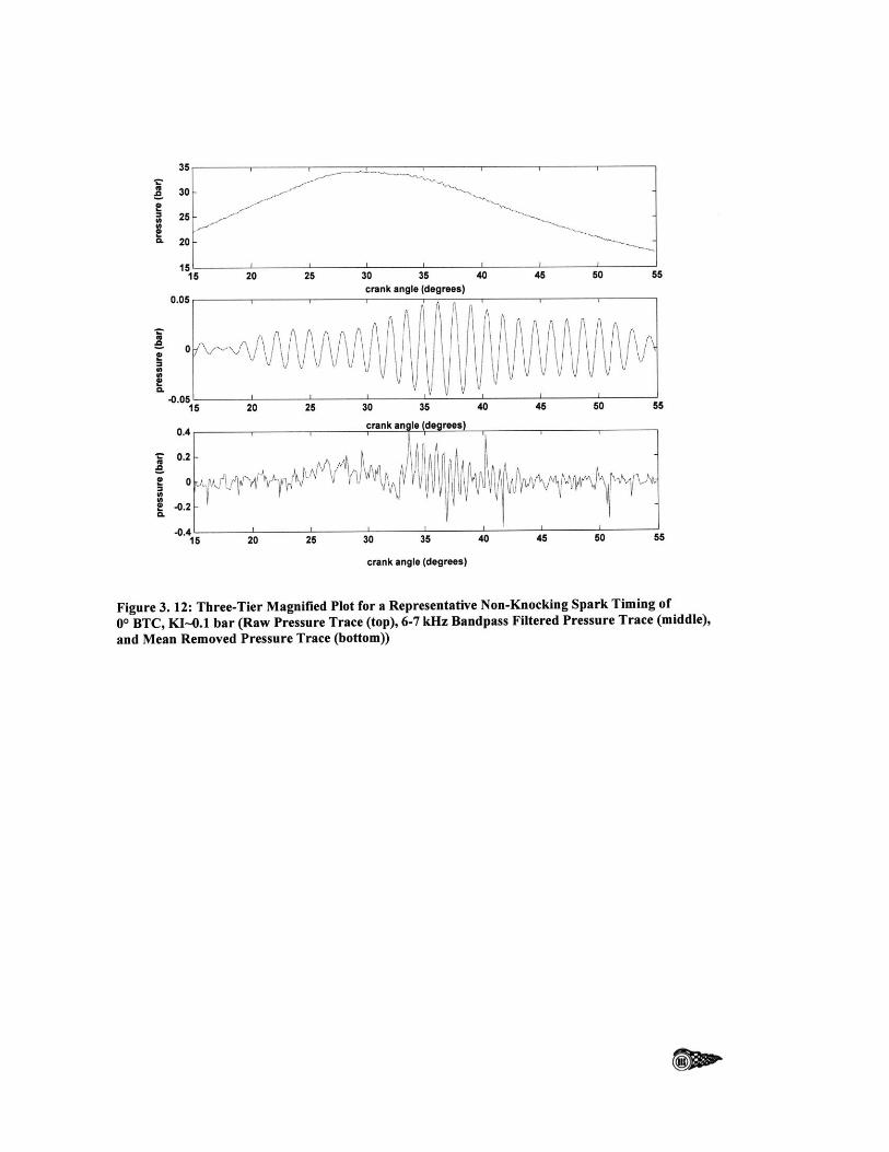
3.2.3 Data Analysis Method for Cylinder Pressure without FilteringFigure 3. 12, Figure 3. 13, and Figure 3. 15 show three-tier magnified plots relating the

raw pressure trace (top), 6-7 kHz bandpass filtered pressure trace (middle), and mean

removed pressure trace (bottom). The range for the bandpass filtered pressure trace was

chosen as it is the first resonant frequency of knock for this engine. Its presence also

becomes more and more significant as the level of knock increases.

42

TRF95

30-

25-

20-

15 20 25 30 35 40 45 50 5crank angle (degrees)

flR A

5

\J \i /

ir f 1" A A

n. R

20 25 30 35 40 45 50 55

15 20 25 30 35 40 45 50 55

crank angle (degrees)

Figure 3. 12: Three-Tier Magnified Plot for a Representative Non-Knocking Spark Timing of

00 BTC, KI~0.1 bar (Raw Pressure Trace (top), 6-7 kHz Bandpass Filtered Pressure Trace (middle),

and Mean Removed Pressure Trace (bottom))

U

.0

e

UInea.

0

1CU,

C.

1C

CL

0

0.051I I

0.4

0.2

0

-0.2


VI N 4IN %"'kA '

"j Ii iVi1VII V

.

50

40

30 -

20 -

101 2 L L 4 4L j15 20 25 30 35 40 45 50 5crank angle (degrees)

0.2 - -

0.1 A 5 I I V 1kJ

-0.1 - V

-0.21 L I

i5 20 25 30 35 40 45 50 5

1- crank angle (degrees)

0.5-

-05-.5 20 25 30 35


5

5

40 45 50 55

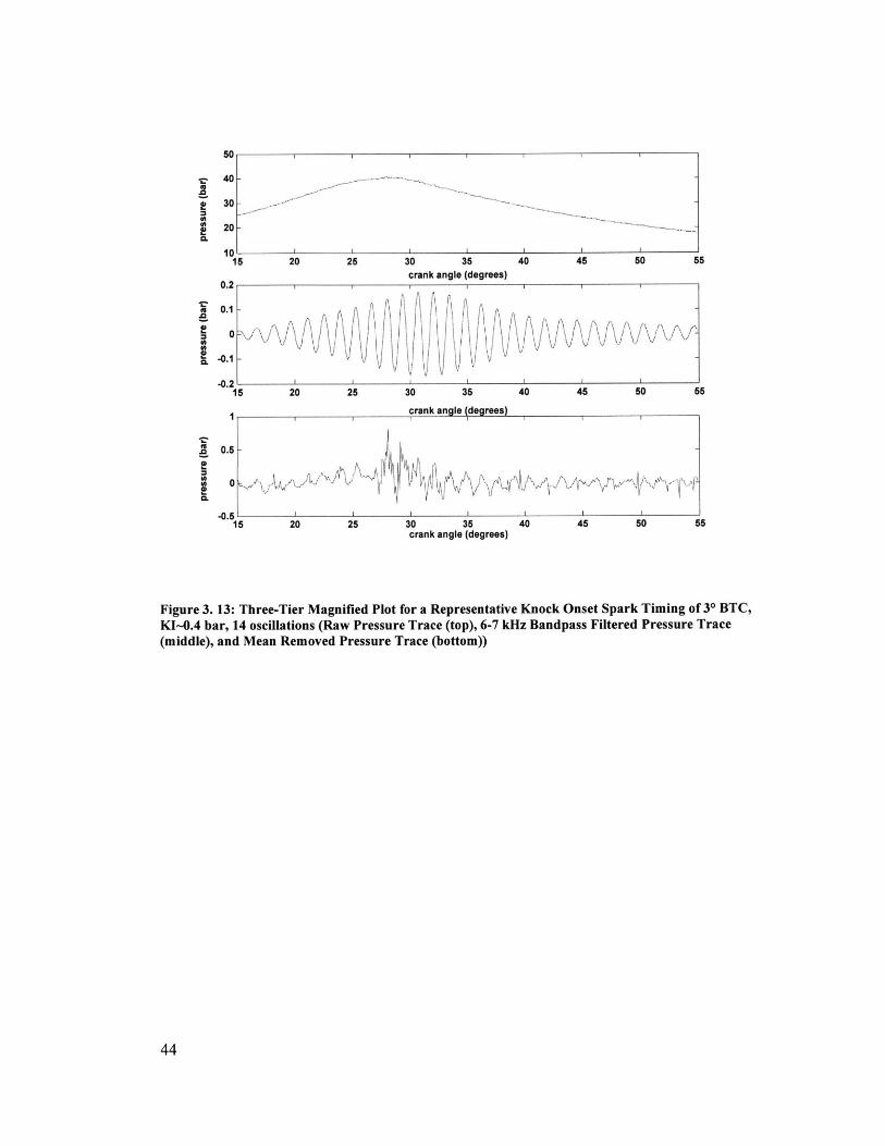
Figure 3. 13: Three-Tier Magnified Plot for a Representative Knock Onset Spark Timing of 3* BTC,KI~0.4 bar, 14 oscillations (Raw Pressure Trace (top), 6-7 kHz Bandpass Filtered Pressure Trace(middle), and Mean Removed Pressure Trace (bottom))

44

a 40-

30-

-. 20- -


1

0.5- \

0.

36 -0.5 -

115 20 25 30 35 40 45 50 55

4 crank angle (degrees)

r 2- -2J 0

II

! -2-a.

-4 L15 20 25 30 35 40 45 50 55


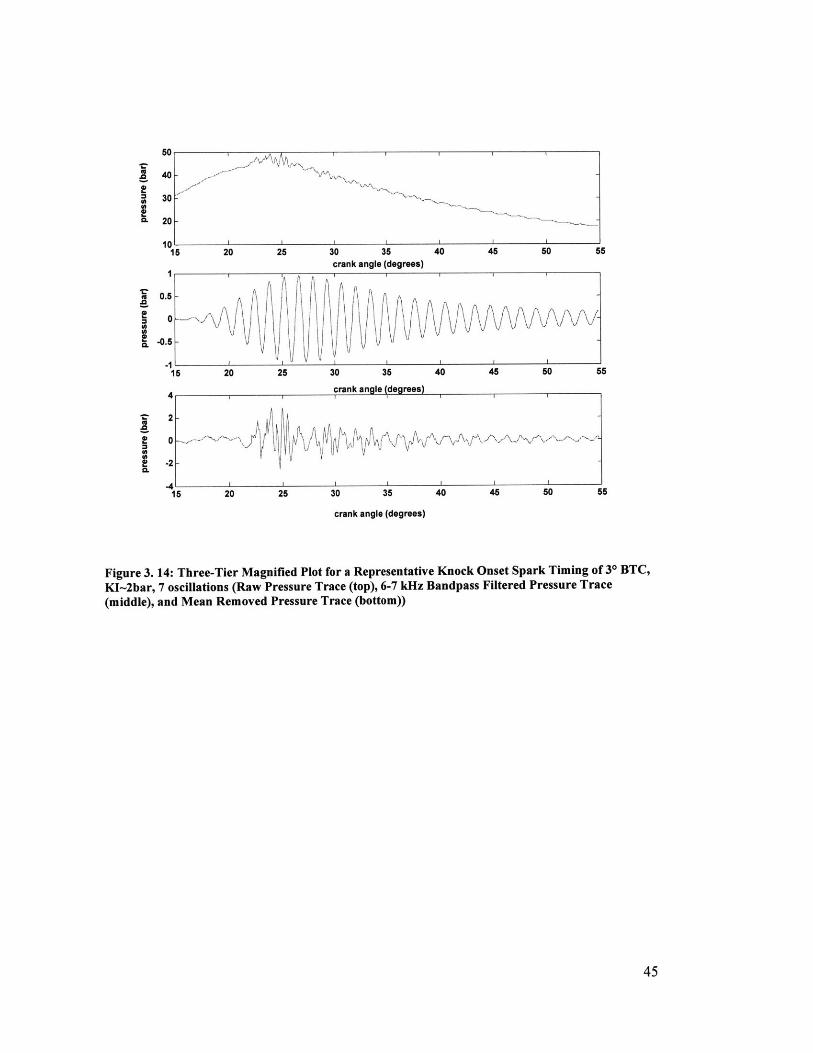
Figure 3. 14: Three-Tier Magnified Plot for a Representative Knock Onset Spark Timing of 3* BTC,

KI-2bar, 7 oscillations (Raw Pressure Trace (top), 6-7 kHz Bandpass Filtered Pressure Trace

(middle), and Mean Removed Pressure Trace (bottom))

45

60 20 25 3 3I 4 4550

20- 2. 2. ....4..4......5CL

0- -


Fiue3 5:TreTe Mgife Ptfr HeiyKnkigSprTiigf6*BCKI2b,

-0.5- 1 A A

-1 .0. IV I

15 20 25 30 35 40 45 50 5

R4ecrank angle (degrees)

~. 2

-2

15 20 25 30 35 40 45 50 55


Figure 3. 15: Three-Tier Magnified Plot for a Heavily Knocking Spark Timing of 60 BTC, Ki-2 bar,7 oscillations (Raw Pressure Trace (top), Bandpass Filtered Pressure Trace (middle), and MeanRemoved Pressure Trace (bottom))

In using the three-tier plots, it was revealed that the 6-7 kHz bandpass filtered pressure

trace shows an autoignition initiation earlier than that expected from either the raw

pressure trace or the mean removed pressure trace. Additionally, in the mean removed

pressure trace plots, the presence of multiple frequency bands was highlighted. Along

with the presence of multiple frequency bands, the mean removed pressure traces outline

rough regions where certain frequencies exist. In cycles that obviously exhibit

characteristics of autoignition that lead to engine knock, such as that in Figure 3. 15, there

is a strong prevalence of the 6.5 kHz signal from the crank angle of knock onset and

continuing on through the pressure trace. In addition to this lower frequency signal, there

is an overlay of higher level frequencies on top of the lower frequency. High frequency

signals exist throughout the entire pressure traces, but their amplitude rises sharply in the

region immediately following the crank angle of knock onset. These higher level

46

frequencies, however, fade after a short period of time down to only the 6.5 kHz signal.

The number of crank angles it takes for the higher level frequencies to die down is shorter

for cycles that lead to heavier engine knock.

The initiation of the multiple frequency oscillations in the mean removed pressure trace

usually coincides quite well with the initiation of the rise in amplitude of the band pass

filtered signal. In cycles that do not have autoignition events that lead to engine knock

such as those in Figure 3. 12, the higher level frequencies often still have a sharp rise near

the same point where the amplitude in the band pass filtered signal also rises, but in these

non-knocking cycles, the higher level frequencies do not fade into a 6.5 kHz signal but

maintain a higher frequency throughout. With cycles that have autoignition events that

lead to heavier engine knock, the higher level frequencies fade into an even smoother and

more regular 6.5 kHz signal.

A pseudo knock intensity can be determined for the mean removed pressure traces by

subtracting the minimum pressure from the maximum pressure. When using this

particular method with this adjusted pressure trace, there is no guarantee that the

maximums and minimums will be very close to each other, hence, the use of the word

pseudo knock intensity. This is due to the multiple frequencies seen from using the three-

tier plots. At the extreme non-knocking and heavy knocking ends, the pseudo knock

intensity has a relatively clear trend. It shows that very small pseudo knock intensities

mean the cycle did not contain an autoignition event leading to engine knock and very

large pseudo knock intensities mean the cycle did contain an autoignition event leading to

engine knock. This trend is not accurate with mid-range pseudo knock intensities and the

status of the cycle could lean towards either non-knocking or knocking; therefore, a

pseudo knock intensity cannot be used to determine engine knock without additional

information.

All of the information just presented can be combined in order to show a progression

through the transition from non-knocking conditions to heavily knocking conditions. For

non-knocking conditions, on a mean removed pressure trace, there is no distinct jump in

47

the pseudo knock intensity level showing an autoignition initiation point. This trace does

not have any areas with distinct frequencies. The entire trace appears to be full of noise.

As the knock onset point is approached, a few cycles will begin to have characteristics

more like those seen in the knock onset cycles including higher jumps in pseudo knock

intensity level. With the exception of a few random cycles that are not able to maintain

engine and head vibrations strong enough to create an audible knock event, these cycles

do not contain the 6.5 kHz signal late in the trace that appears at the knock onset point.

At knock onset, using the mean removed pressure traces, an autoignition initiation point

can be identified where there is a sudden jump in the pseudo knock intensity level. At

this point, there is also the presence of more than one frequency in the signal for a short

period of time, roughly 5-10 crank angle degrees. This period of multiple frequencies

quickly fades to a signal that only contains the 6.5 kHz frequency after a short period of

time in those cycles that contain autoignition events that lead to engine knock.

Depending on the octane rating of the fuel used, the percentage of cycles that behave in

this manner at the knock onset conditions ranges from 5-50%. Those cycles that do not

show autoignition events that lead to engine knock either look like those described in the

paragraph above regarding non-knocking cycles or have an appearance somewhere

between these two descriptions. These cycles will still contain the multiple frequencies

for a short period of time with a less distinct beginning, but will not fade into a clear 6.5

kHz signal. The presence of higher order frequencies persists.

For heavier knocking conditions, on a mean removed pressure trace, the sudden jump in

the pseudo knock intensity level is even greater than that seen at knock onset conditions.

The larger amplitudes in these signals make the noise before the autoignition initiation

point much less significant; however, the multiple frequencies are still easily seen for a

short period of time, roughly 5-10 crank angle degrees, before they fade to only the 6.5

kHz signal. Again, because of the larger amplitude, this 6.5 kHz signal will actually

appear to be smoother and contain less noise.

48

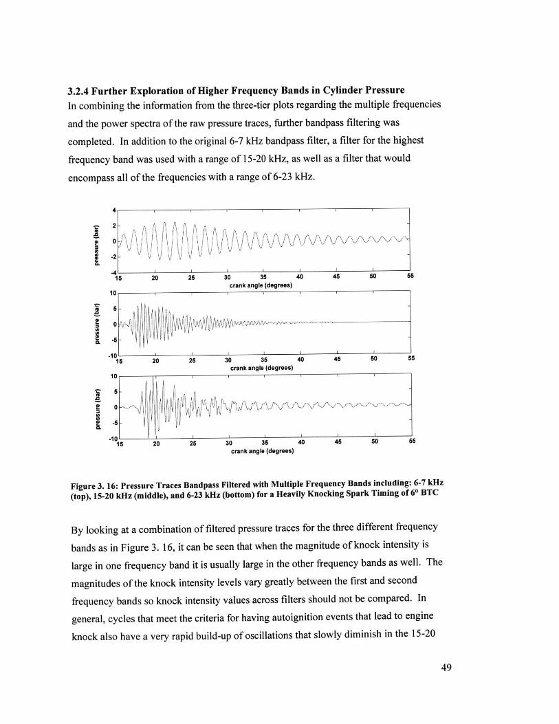
3.2.4 Further Exploration of Higher Frequency Bands in Cylinder Pressure

In combining the information from the three-tier plots regarding the multiple frequencies

and the power spectra of the raw pressure traces, further bandpass filtering was

completed. In addition to the original 6-7 kHz bandpass filter, a filter for the highest

frequency band was used with a range of 15-20 kHz, as well as a filter that would

encompass all of the frequencies with a range of 6-23 kHz.

2- ! I A

0

415 20 25 30 35 40 45 50 55

crank angle (degrees)'10-

5-

. -5-

_10- L


10

. 5-

pil 0-----0

CL 10 I15 20 25 30 35 40 45 50 55


Figure 3. 16: Pressure Traces Bandpass Filtered with Multiple Frequency Bands including: 6-7 kHz

(top), 15-20 kHz (middle), and 6-23 kHz (bottom) for a Heavily Knocking Spark Timing of 60 BTC

By looking at a combination of filtered pressure traces for the three different frequency

bands as in Figure 3. 16, it can be seen that when the magnitude of knock intensity is

large in one frequency band it is usually large in the other frequency bands as well. The

magnitudes of the knock intensity levels vary greatly between the first and second

frequency bands so knock intensity values across filters should not be compared. In

general, cycles that meet the criteria for having autoignition events that lead to engine

knock also have a very rapid build-up of oscillations that slowly diminish in the 15-20

49

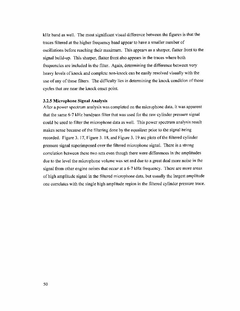
kHz band as well. The most significant visual difference between the figures is that the

traces filtered at the higher frequency band appear to have a smaller number of

oscillations before reaching their maximum. This appears as a sharper, flatter front to the

signal build-up. This sharper, flatter front also appears in the traces where both

frequencies are included in the filter. Again, determining the difference between very

heavy levels of knock and complete non-knock can be easily resolved visually with the

use of any of these filters. The difficulty lies in determining the knock condition of those

cycles that are near the knock onset point.

3.2.5 Microphone Signal AnalysisAfter a power spectrum analysis was completed on the microphone data, it was apparent

that the same 6-7 kHz bandpass filter that was used for the raw cylinder pressure signal

could be used to filter the microphone data as well. This power spectrum analysis result

makes sense because of the filtering done by the equalizer prior to the signal being

recorded. Figure 3. 17, Figure 3. 18, and Figure 3. 19 are plots of the filtered cylinder

pressure signal superimposed over the filtered microphone signal. There is a strong

correlation between these two sets even though there were differences in the amplitudes

due to the level the microphone volume was set and due to a great deal more noise in the

signal from other engine noises that occur at a 6-7 kHz frequency. There are more areas

of high amplitude signal in the filtered microphone data, but usually the largest amplitude

one correlates with the single high amplitude region in the filtered cylinder pressure trace.

50

0.1.0

0 50 100 150

0

01 50 100 150

001,~

0 50 10 15

crn an0.(eres

0.2

0

0 50 100 150

0

0 50 100 150

0

0 50 100 150

0

0 50 100 150crank angle (degrees)

0.1

0-01I0 50 100 150

0.1 A0

-0

0 50 100 150

0.1

0

0 50 100 150


Figure 3. 17: Cylinder Pressure Trace Superimposed over Microphone Signal for a Non-Knocking

Spark Timing of 00 BTC

51

0.5

-0.50 50 100 150

0.2

0

-0.2

0 50 100 150

0.40.2

0

-0.4

0 50 100 150

0 50crank angle (degrees)

0.2

0

-0.2WV

0 50 100 150

0.4

0.2

02-0.4

0 50 1045

0 50 100 150

0.2

0

-0.2

0 50 100 150


04

0 50 100 150

0.2

02-0.4

0 50 100 150


Figure 3. 18: Cylinder Pressure Trace Superimposed over Microphone Signal at the Knock OnsetSpark Timing of 3 BTC

52

C)

U)

2

a

0L

-1

0

0 50 100 150

0 50 100 150

1 ' '

-1

0 50 100 150

1 c

0 50 100 150

2

-21


0

-210 50 100 150

1

-1 , , , .

0 50 100 150

0.5

-0.5

0 50 100 150

1

1

-1 ,0 50 100 150


Figure 3. 19: Cylinder Pressure Trace Superimposed over Microphone Signal for a HeavilyKnocking Spark Timing of 60 BTC

Additionally, the microphone data and cylinder pressure were compared by plotting

cylinder pressure knock intensities versus microphone knock intensities. Microphone

knock intensity was calculated using the same method as that for cylinder pressure knock

intensity. An example of a partial set of these plots can be found in Figure 3. 20, Figure

3. 21, and Figure 3. 22 while those for all of the octane ratings can be found in the

appendix. A linear trendline was then fit to each set of data as well as an R2 value for

each of the trendlines. Spark timings that are non-knocking have relatively low R2 values

for these trendline equations. When the spark timing of knock onset is reached, the R2

value for the linear equation jumps to a higher value that is in the region or greater than

0.85. This shows a much more substantial linear relationship develops between the

microphone knock intensity and the cylinder pressure knock intensity as knock onset is

53

10

0 50 100 150

0.4

0.2

-0.2

-0.40 50 100 150

2

-2

0 50 100 150

2

0


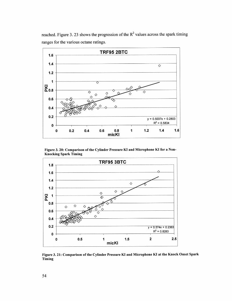
reached. Figure 3. 23 shows the progression of the R2 values across the spark timing

ranges for the various octane ratings.

1.6

1.4

1.2

1

0.8

0.6

0.4

0.2

00 0.2 0.4 0.6 0.8

micKI1 1.2 1.4 1.6

Figure 3. 20: Comparison of the Cylinder Pressure KI and Microphone KI for a Non-Knocking Spark Timing

1.8

1.6

1.4

1.2

0.I

0.8

0.6

0.4

0.2

00 0.5 1 1.5 2 2.5

micKI

Figure 3. 21: Comparison of the Cylinder Pressure KI and Microphone KI at the Knock Onset SparkTiming

54

.

TRF95 2BTC

y = 0.5037x + 0.2803R2 = 0.5834

TRF95 3BTC

0 V

y = 0.574x + 0.2363R2 = 0.8283

2.5

2

1.5

1

0.5

00 0.5 1 1.5

micKI

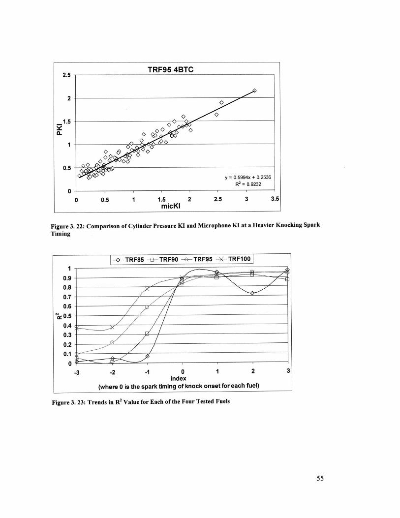
Figure 3.Timing

2 2.5 3 3.5

22: Comparison of Cylinder Pressure KI and Microphone KI at a Heavier Knocking Spark

+T RF85 -49- TRF90 ,-e- TRF95 -X- T RF100

0.90.80.70.6

S0.50.4

0.3

0.20.1

0

-3 -2 -1 0 1 2 3index

(where 0 is the spark timing of knock onset for each fuel)

Figure 3. 23: Trends in R2 Value for Each of the Four Tested Fuels

TRF95 4BTC

y = 0.5994x + 0.2536R2 = 0.9232

-

55


56

CHAPTER 4: SUMMARY AND CONCLUSIONS

The data presented in this work confirms that the cylinder pressure signal contains

multiple frequencies of interest. The first is near 6.5 kHz which is the resonant frequency

of the cylinder. Another is near 17.5 kHz which is close to the third harmonic of the

resonance frequency. While filtering is useful, using a smoothing technique to find a

mean pressure trace and then subtracting it from the original pressure trace may be an

adequate means of data processing for evaluation of the data.

Using either bandpass filtered data or mean removed pressure data, a knock intensity can

be determined that gives significant insight into the type of autoignition event that may

have occurred during a cycle and whether or not that autoignition event will lead to

engine knock. Microphone signal data can also be bandpass filtered and knock intensities

can be calculated from this data also providing information on the type of autoignition

during a cycle. This bandpass filtered microphone data has similar bursts of oscillations

to those found in the bandpass filtered pressure traces.

The figures regarding the number of oscillations before peak in a bandpass filtered

pressure trace support the ideas from previous work that the end gas contains one or more

hot spots that autoignite causing pressure gradients that can trigger rapid pressure

oscillations. These pressure oscillations can cause block and head vibrations that lead to

audible noise outside the engine. The number of oscillations before peak amplitude is

related to how rapidly the pressure oscillations are able to build up, while the knock

intensity is related to the amount of energy available for release as noise for that

particular cycle.

The mean removed pressure traces show that there is a gradual build-up to more intense

autoigniting cycles as conditions transition from non-knocking to knock onset and on to

heavier knock. This transition includes a period of higher frequency pressure waves that

set up the autoignition process, presumably in a similar manner to those seen in the video

frames from Pan and Sheppard [7]. These higher frequency pressure waves then decay to

a single base frequency of 6.5 kHz for the tests completed in this work.

57

There are three promising methods that could potentially be used in for determining

knock onset without the need to have an operator constantly sitting at the engine and

listening. The first uses plots of the knock intensity versus the number of oscillations

before the peak of a lowest frequency (in this instance a 6-7 kHz) bandpass filtered

pressure trace. On these plots, cycles begin to appear in the region of KI greater than 1

bar and a short 5-10 oscillation build-up to peak. The second method looks at the

average KI over all the cycles and the average (dP/dO)max over all cycles. Using the data

taken thus far, trends have shown that knock onset correlates with an average KI of-0.4

bar and an average (dP/d)max of-10 bar/ 'CA. The third possible method uses the R2

values from linear trendlines on plots of cylinder pressure knock intensity versus

microphone signal knock intensity. As the R2 value takes a jump from distinctively

lower values into a region of values greater than 0.85, knock onset occurs.

Future work should consist of more extensive microphone signal testing and analysis as

well as an expansion of test fuels. Additional microphone data is needed to confirm the

relationship between the various knock intensities. Moving the microphone to various

locations around the outside of the engine including different heights could possibly give

insight into where the end gas or hot spots might be more prevalent and may lead to a

better description of what is physically taking place in the cylinder. Further processing of

the microphone data in various manners could also be done in order to look for any

further in-cylinder details. As for fuels, in addition to the TRFs tested, PRFs should also

be investigated in order to determine if the same trends are seen for a different type of

fuel. Once trends have been confirmed with PRFs, unleaded test gasolines of various

octane ratings should be used in order to confirm that fuels more like those used in the

real world also behave as predicted.

58

REFERENCES

[1] Heywood, J.B., Internal Combustion Engine Fundamentals, McGraw Hill Inc.,New York, 1988.

[2] Lee, J., Hwang, S., Lim, J., et al., "A New Knock-Detection Method usingCylinder Pressure, Block Vibration and Sound Pressure Signals from a SIEngine," SAE 981436.

[3] Kaneyasu, M., et al., "Engine Knock Detection Using Multi-Spectrum Method,"SAE 920702.

[4] Chiriac, R., Radu, B., and Apostolescu, N., "Defining Knock Characteristics andAutoignition Conditions of LPG with a Possible Correlation for the ControlStrategy in a SI Engine," SAE 2006-01-0227.

[5] Grandin, B., Denbratt, I., et al., "Heat Release in the End-Gas Prior to Knock inLean, Rich and Stoichiometric Mixtures With and Without EGR," SAE 2002-01-0239.

[6] Bradley, D., Morley, C., et al., "Amplified Pressure Waves During Autoignition:Relevance to CAI Engines," SAE 2002-01-2868.

[7] Konig, G. and Sheppard, C.G.W., "End Gas Autoignition and Knock in a SparkIgnition Engine," SAE 902135.

[8] Pan, J. and Sheppard, C.G.W., "A Theoretical and Experimental Study of theModes of End Gas Autoignition Leading to Knock in S.I.Engines," SAE 942060.

[9] Topinka, J., Knock Behavior of a Lean-Burn, H2 and CO Enhanced, SI GasolineEngine Concept, M.S. Thesis, MIT, May 2002.

[10] Gerty, M.D., Effects of Operating Conditions, Compression Ratio, and Gasoline,Reformate on SI Engine Knock Limits, M.S. Thesis, MIT, May 2005.

59


60

APPENDIX: ADDITIONAL FIGURES

61

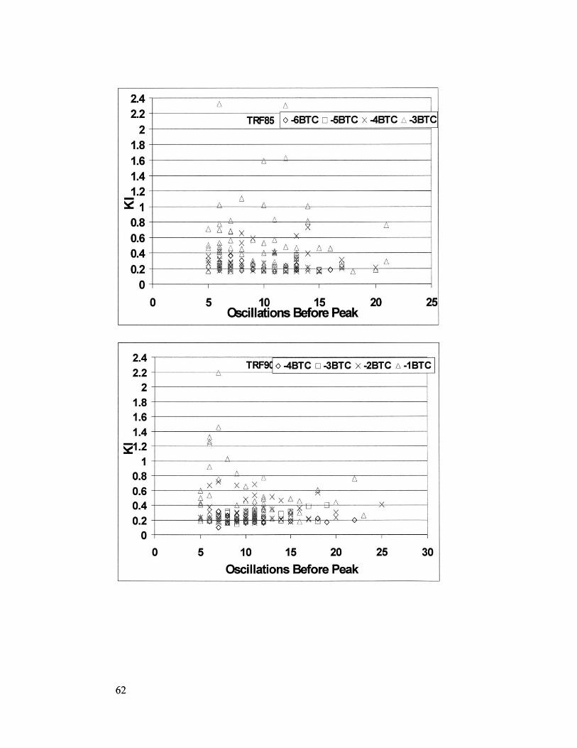
2.4

2.2 TRF85 -6BTC -6BTCx -4BTC -3BTC2-

1.8-1.6- A

1.4-1.2-

0.8-0.6- AXAL

0.4 -0.2-

0- 1

0 5 10 15 20 25Oscillations Before Peak

2.4-TRF9( o -4BTC E -3BTC x -2BTC A -1BTC

2.22

1.81.61.4 -

21.2'1 A^

0.8 ^ Ax xx0.6 A A

0.4-A XA~

0.2 - -A

0-

0 5 10 15 20 25 30Oscillations Before Peak

62

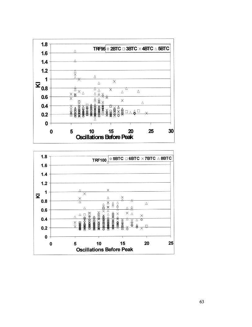
1.8

1.6 T9 2TC 3BTC x 4BTCA 5BTC

1.4 A

1.2 21 x

x A

A

I - -C. A X-

X14 XR A X( A A A

AA

00 5 10 15 20 25 30

Oadilltons Before Peak

1.8 - -- T RF 00 o 5BTC n 6BTC x 7BTC L, 8BTC

1.6 -

1.4

1.2A X x

x A x0.8

0.6-ILM x n x

0.4- Z A A

0.2-

0-0 5 10 15 20 25


63

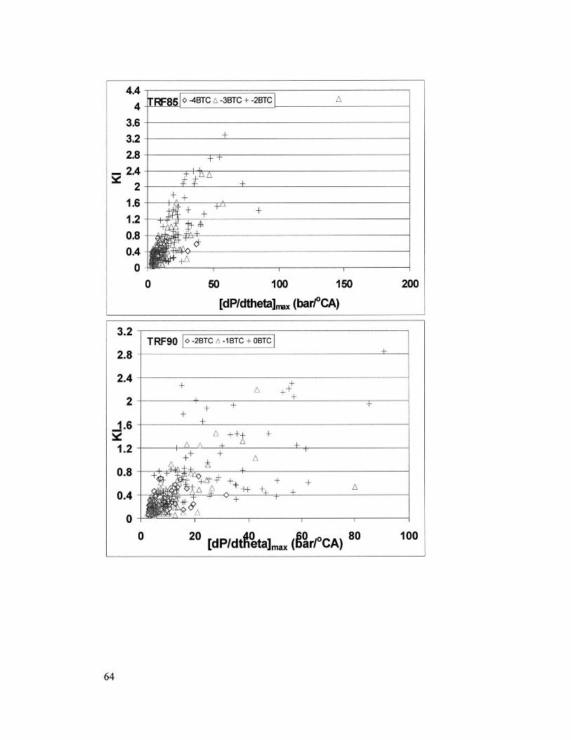
4.44

3.63.22.8

. 2.4

1.61.2

0.80.4

00 6c 100 1

[dP/dtheta]m. (bar/*CA)

50 200

3.2TRF90 1 -2BTC A -1BTC + OBTC

2.8

2.4 -

2 ++ ++

1.6- +

1.2 - wN +++. + ++

0.8 + +

0.4A +

0

0 20 [dP/dteta]mx(gar/oCA) 80 100

64

+

A

+ +

+

A +^+

& m

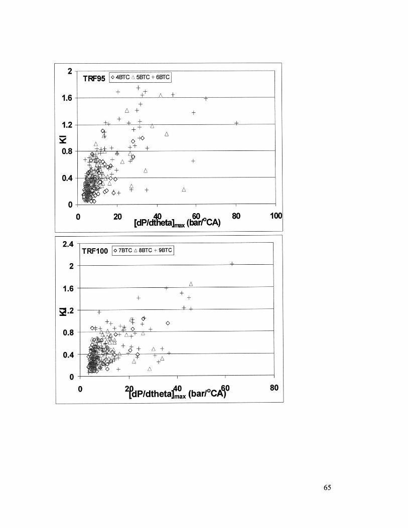
20 [ d 60[dP/dtheta,. (bareCA)

2fdP/dtheta1- (bar/OCAD

2TRF95 1 4TC A 5BTC + 6BTC

+ A +

+

+

+ + LALi+

+A

++

++ AI

1.6

1.2

0.8

0.4

0

0

2.4

2

1.6

0.8

0.4

0

80 100

TRF100 107BTC A8 BTC + 9BTC

++

+ + +-++

A +A

+1+A-

0 80

65

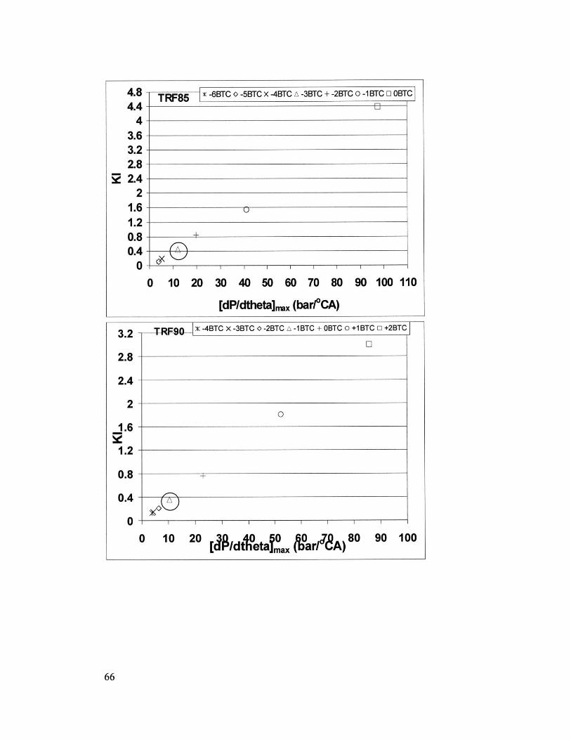
4.8 TRF85 -6BTC 0 -5BTC x -4BTC A -3BTC + -2BTC O -1BTC OBTC

4.4 L4

3.63.22.8

S2.42

1.6-1.20.8+0.4-0 - I I I I

0 10 20 30 40 50 60 70 80 90 100 110

[dP/dtheta]fx (bar/*CA)

3.2 7-- X -4BTC x -3BTC 0 -2BTC z -1BTC + OBTC o +1BTC 0 +2BTC

2.8

2.4

2

1.6

1.2

0.8

0.4

0

0 10 20 [0dt4 etam (arI eA) 80 90 100

66

0

I Ii i i i

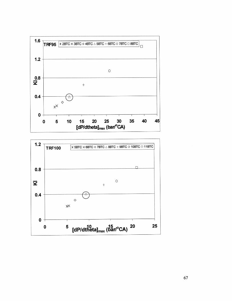
1.6

1.2

0.8

0.4

0

0 5 10 15 20 25 30[dP/dtheta]J (bar/*CA)

35 40 45

1.2

0.8

0.4

025205 [P 0m ( *

[dP/dtheta~max (br/ CA)0

TRF95 r) BCX3T BCA5T BC07T BCIF

0

0+

6:X

TRFIOO K5BTCX 6BTCc07BTC A 8BTC+9BTCO O1BTC E 11BTC

0

/"A

x)

67

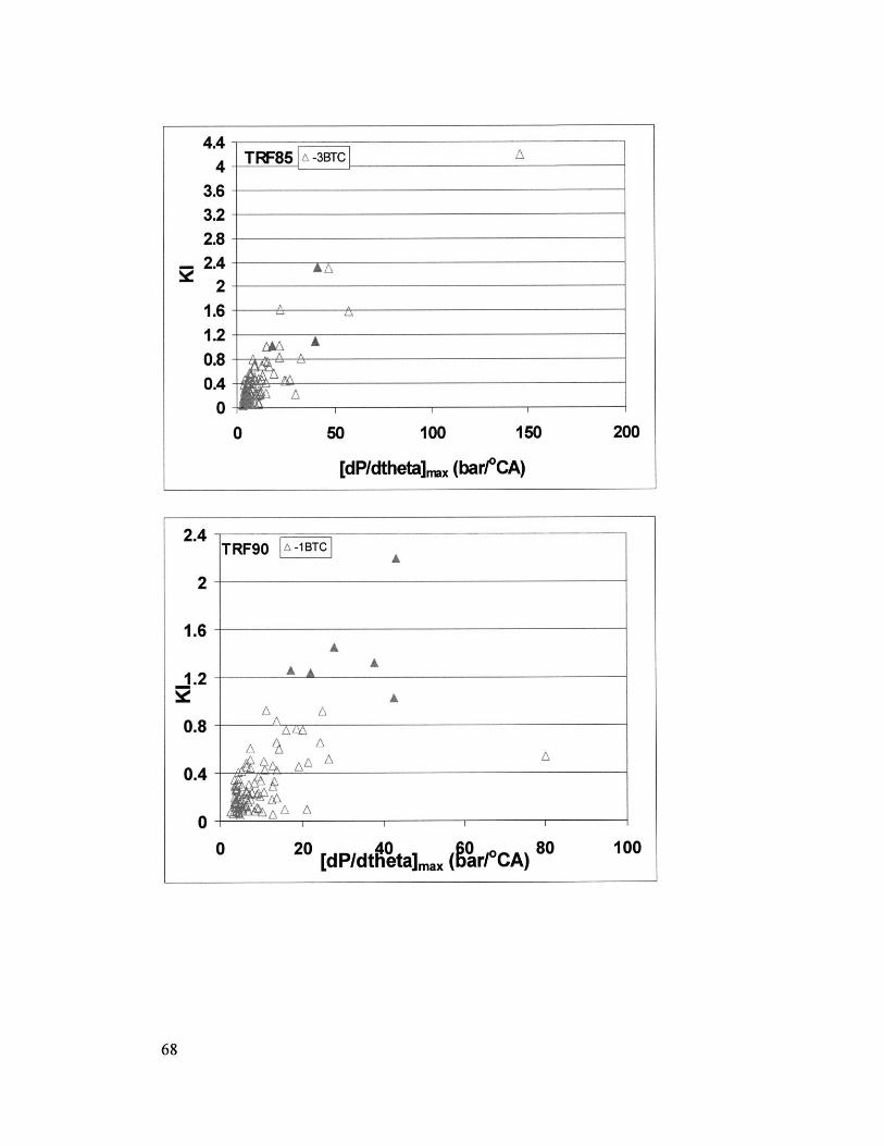
4.44 TRF86 F a-3rc

3.6-3.22.82.4- AA

2-

1.6 -1.2

A A\ A0.8 A A

0.40

0 50 100 150 200

[dP/dtheta]J. (bar/*CA)

2.4TRF90 -

2A

1.6A

1.2 AAA

A A

0.4 -

0 2\ I ( CA

0 20 t40 60 80 100EdPldthetamax (arI 0CA)

68

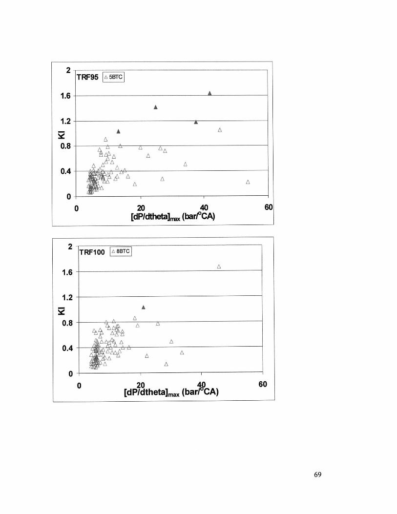
20[dP/dtheta]nm

2

1.6

1.2

0.8

0.4

00

TRF95 A5BTC

A

A

AA AAAA A

A t~

. A A-A

40(bar/*CA)

60

2TRF100 L 8BTC

1.6 A

1.2

A

0.8 AA AA

0.4

0

0 20 40 60[dP/dtheta]max (barl"CA)

69

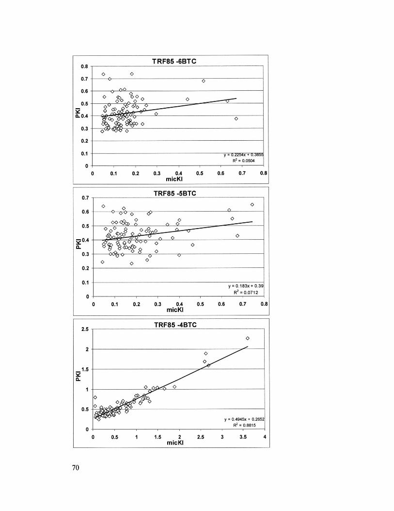
TRF85 -6BTC0.8

0.7

0.6 0

0.5

CL 0.4

0. 3

0.2

0.1 y =0.2254X + U.3U55R2 = 0.05040

0 0.1 0.2 0.3 0.4 0.5 0.6 0.7 0.8micKI

0.7 - TRF85 -5BTC

0.6 0

0.5 0.6

0.4

0.3

0.2

0.1y = 0.183x + 0.39

R2 = 0.07120

0 0.1 0.2 0.3 0.4 0.5 0.6 0.7 0.8micKi

2.5 TRF85 -4BTC

2

1.5

0.5

y = 0.4945x + 0.2652R2 = 0.8815

01 1

0 0.5 1 1.5 2 2.5 3 3.5 4micKI

70

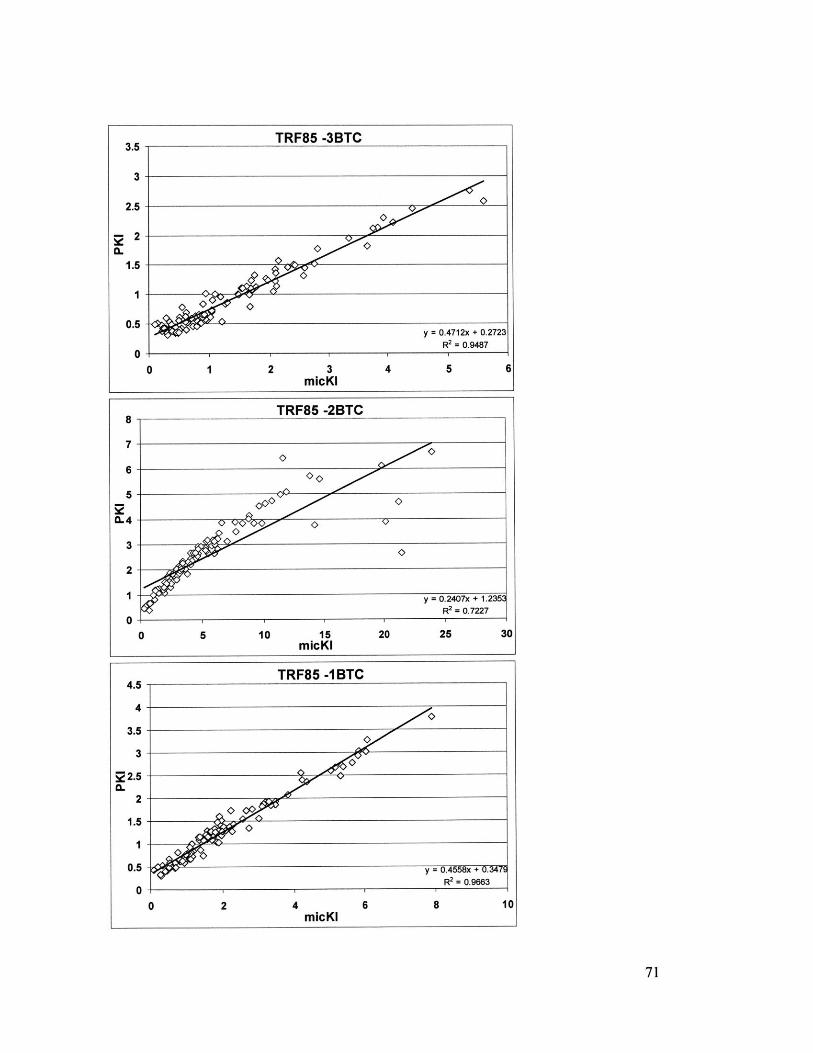
3.5

3

2.5

- 2

1.5

1

0.5

00

TRF85 -3BTC

1 2 3micKi

4 5 6

8 ___ _ TRF85 -2BTC

7.-

6

CL4

3 -, 0 -

2

y =0.2407x + 1.2353R2e 0.7227

00 5 10 15 20 25 30

micKI

TRF85 -1 BTC4.5

4.

3.5

3

22.5

2

1.5

1

0.5 - y =0.4558x + 0.3479R 2 = 0.9663

00 2 4 6 8 10

micKI

71

y = O.4712x + 0.2723R2 = 0.9487

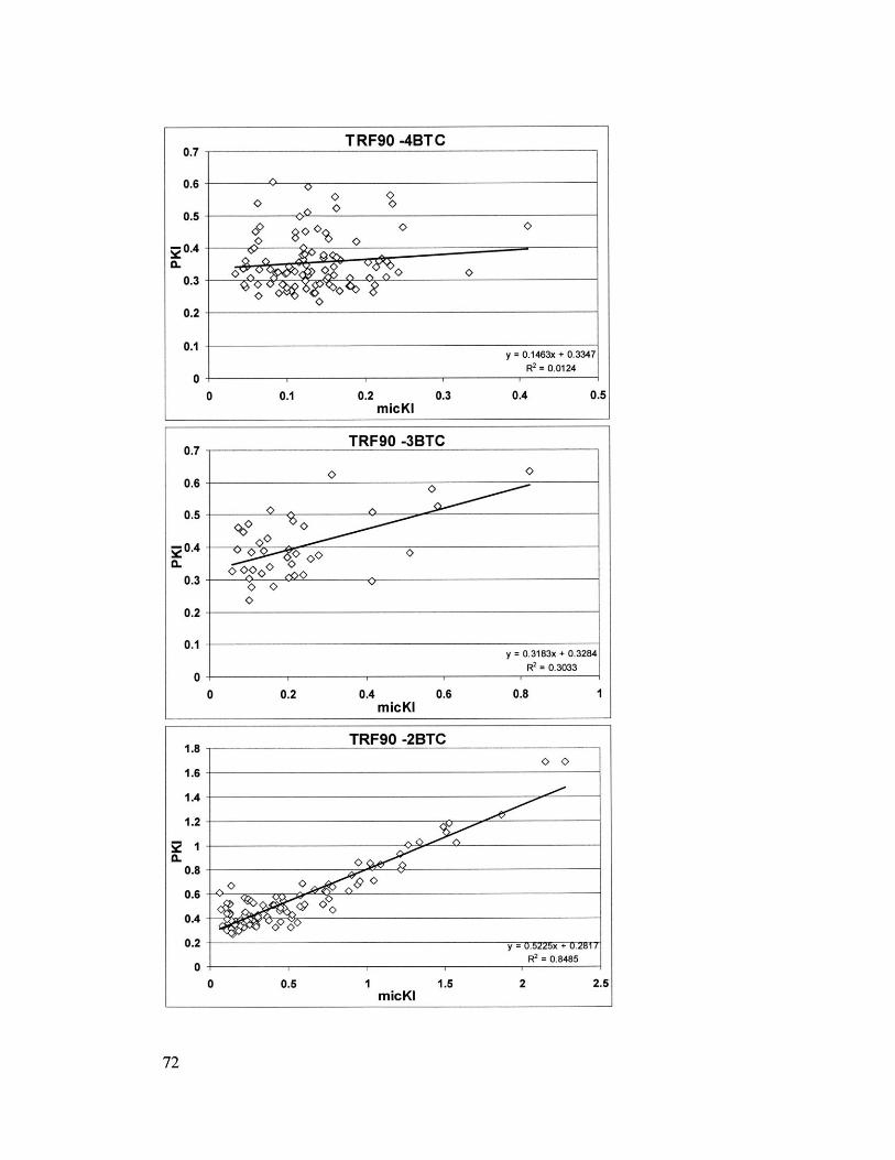
0.7

0.6

0.5

20.4I-

0.3

0.2

0.1

00

0.7

0.6

0.5

0.40.

0.3

0.2

0.1

00

0.1

0.2

0.2

0.4

micKi

micKi

0.3

0.6

0.4

0.8

0.5

1

y 0.5225x + U.281/R2 = 0.8485

0 0.5 ImicKi

1.5 2 2.5

TRF90 -4BTC

09 O>

y = 0.1463x + 0.3347R2 = 0.0124

TRF90 -3BTC

y = 0.3183x + 0.3284R2 = 0.3033

TRF90 -2BTC

0~c

1.8

1.6

1.4

1.2

0.8

0.6

0.4

0.2

0

72

-

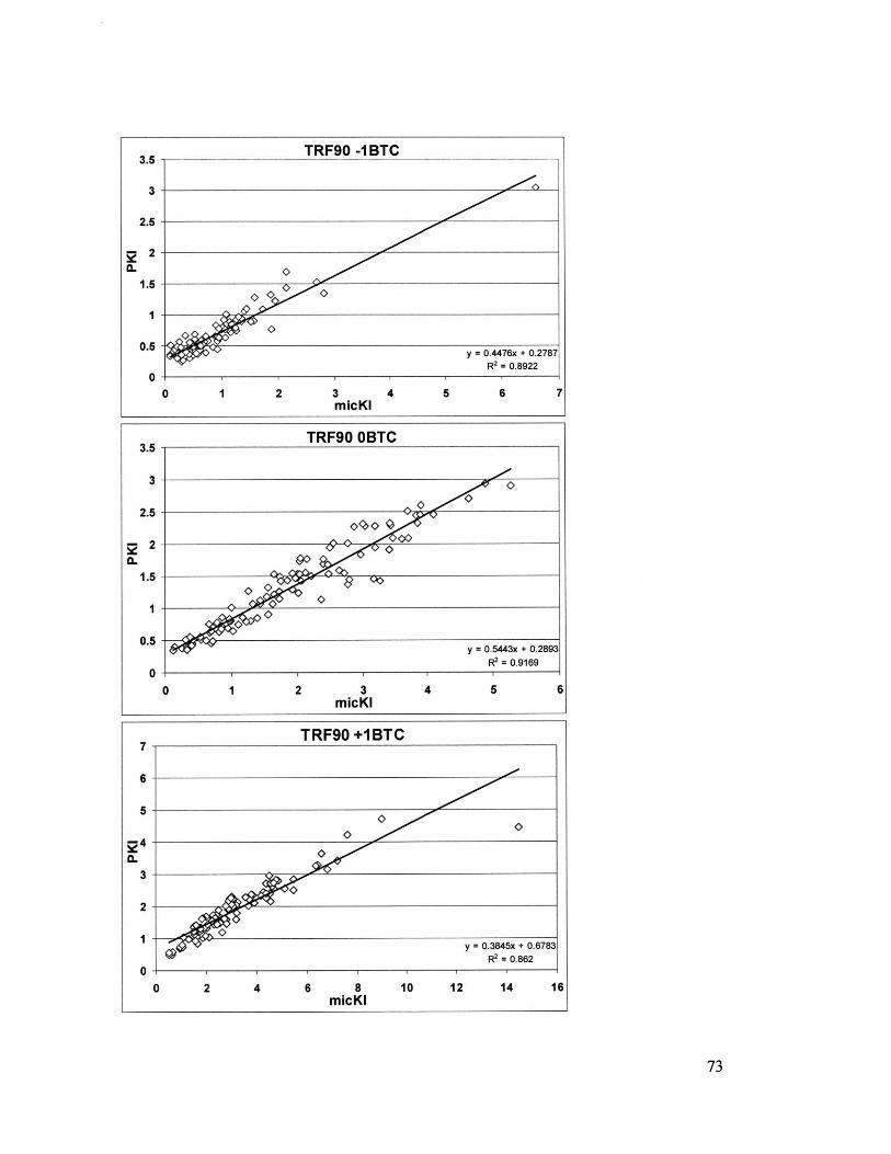
0 1 2 3 4 5 6micKi

0 I 2 3micKi

4 5

7

6

5

3

2

1

00 2 4 6 8

micKi10 12 14 16

3.5

3

2.5

22IL

TRF90 -1BTC__ _

y = 0.4476x + 0.2787R2 = 0.8922

1.5

1

0.5

0

3.5

3

2.5

7

22C-

TRF90 OBTC

y = 0.5443x + 0.2893R = 0.9169

1.5

I

0.5

0

T RF90 +1BT C

6

y = 0.3845x + 0.6783R2= 0.862

73

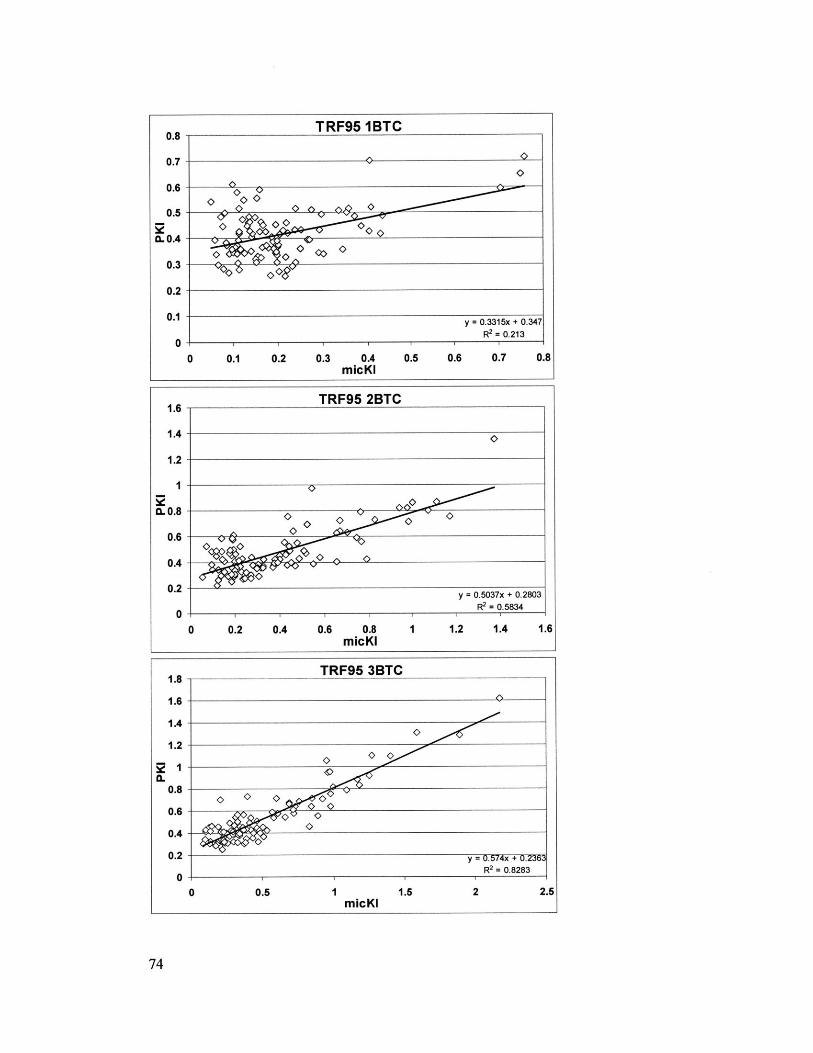
0.8

0.7

0.6

0.5

0.0.4

0.3

0.2

0.1

00 0.1 0.2 0.3 0.4

micKi0.5 0.6 0.7 0.8

1.6 TRF95 2BTC

1.4

1.2

1

CL 0.8 > 00

0.6 C>C>

0.4 -

0.2 y = 0.5037x + 0.2803

o R2 = 0.5834

0 0.2 0.4 0.6 0.8 1 1.2 1.4 1.6micKi

1.8

1.6

1.4

1.2

0.I

0.8

0.6

0.4

0.2

00 0.5 I

micKi1.5 2 2.5

74

TRF95 IBTC

00

y = 0.3315x + 0.347R2= 0.213

------ -- TRF95 3BTC

y =0.574x + 0.2363R 2 = 0.8283

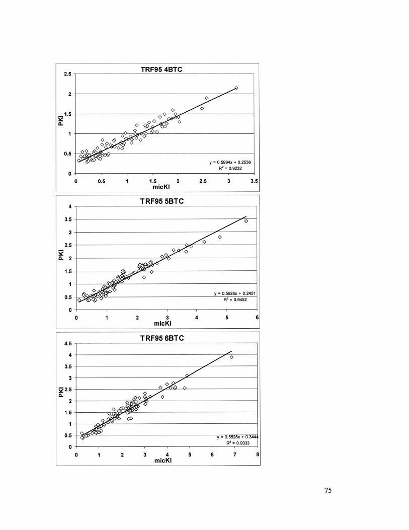
2.5

2

1.5

1

0.5

0

0 0.5 1.5micKi

2 2.5 3 3.5

TRF95 5BTC4

3.5

3

2.5

1.5

1

y = 0.5926x + 0.24510.5 O R2= 0.9452

00 1 2 3 4 5 6

micKi

TRF95 6BTC4.5

4

3.5

3

22.5

2

1.5

0.5

0

y = 0.5528x + 0.344R

2= 0.9333

0 1 2 3 4micKI

5 6 7 8

TRF95 4BTC

y = 0.5994x + 0.2536R2= 0.9232

75

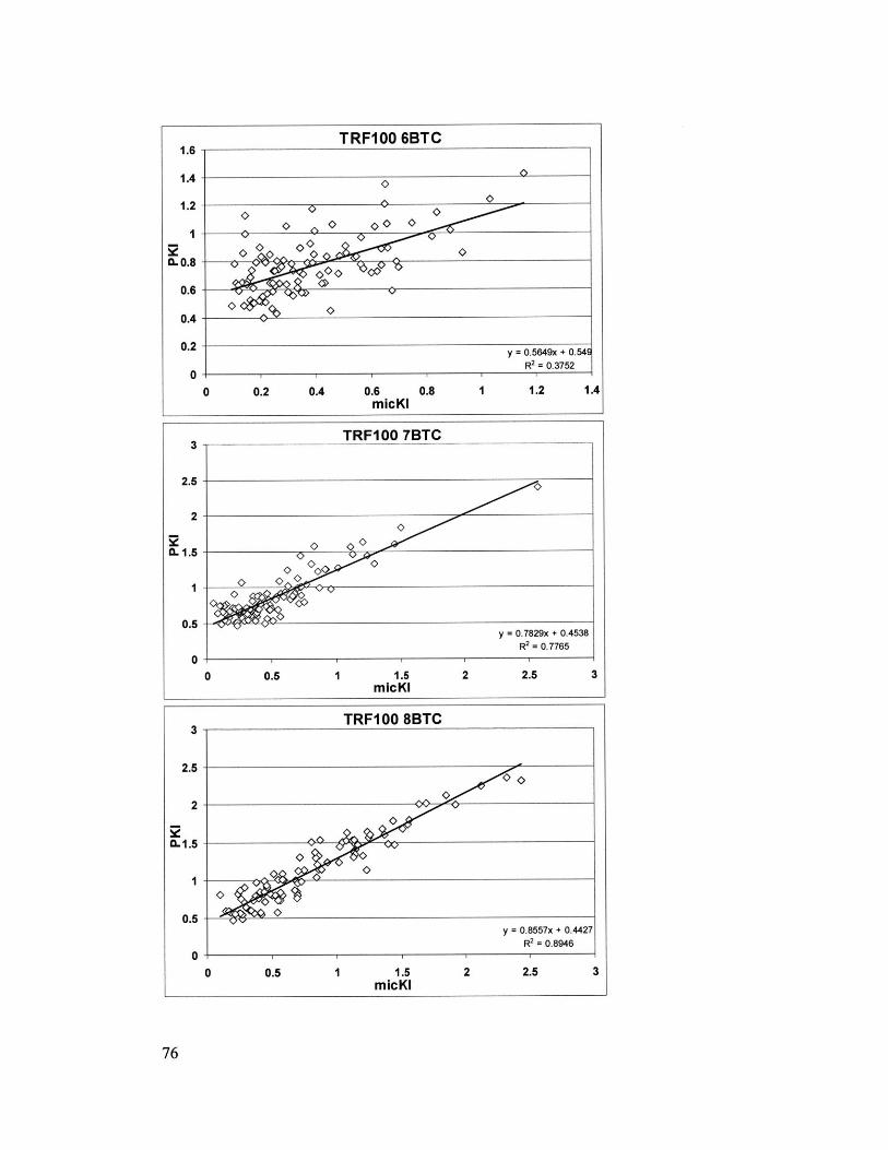
'0

y = 0.5649x + 0.54R2 = 0.3752

0 0.2 0.4 0.6 0.8 1 1.2 1.4micKi

0 0.5 1 1.5micKi

0 0.5 1 1.5micKi

2 2.5 3

2 2.5 3

TRFIOO 6BTC1.6

1.4

1.2

1

IL0.8

0.6

0.4

0.2

0

3

2.5

2

0. 1.5

y = 0.7829x + 0.4538R2 = 0.7765

1

0.5

0

TRFIOO 8BTC3

2.5

2

C0.1.5

1

0.5

0

o' 0

y = 0.8557x + 0.4427R2 = 0.8946

76

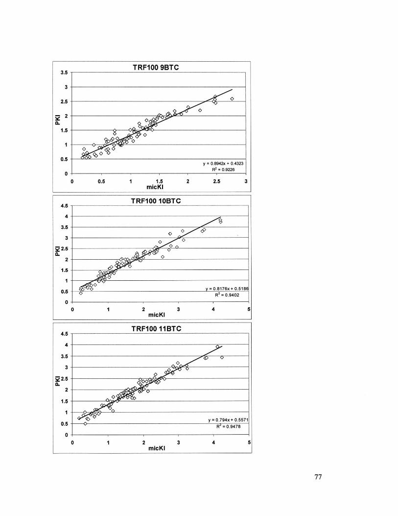
TRF100 9BTC3.5

3

2.5

-2

1.5

0.5y = 0.8942x + 0.4323

R2 = 0.92260

0 0.5 1 1.5 2 2.5 3micKI

TRF100 IOBTC4.5 -

4

3.5

3

22.5 -

2

1.5

I

0.5 y =0.8176x + 0.518R2 0.9402

00 1 2 3 4 5

micKi

TRFIOO 11BTC4.5

4

3.5

3

22.5'a.

2

1.5

y. 0.794x +0.5571R 2= 0.9478

0 1 2 3 4 5micKi

77


78

Documents

PHENOMENA THAT DETERMINE KNOCK ONSET IN SPARK …