Filtered Multitone Modulationand Equalization Techniques

PhD Third Progress Seminar Report

Submitted in the partial fulfillment of the requirements

for the degree of

Doctor of Philosophy

by

Santosh V JadhavRoll No. 02407802

under the guidance of

Prof. Vikram M Gadre

Department of Electrical Engineering

Indian Institute of Technology, Bombay

June 2005

Acknowledgement

I would like to express my sincere gratitude to my guide, Prof. Dr. Vikram M. Gadre for his help

and guidance during the course of my progress seminar. I am also thankful to Dr. K. L. Asanare,

Director, FAMT for his continuous encouragement and support.

I would also like to thank members of ”Modem Group”, Satyam and Chirag for the discussions

we had, which helped a lot during preparation of this seminar.

Santosh V JadhavJune 2005

i

Contents

List of figures iv

Abstract 1

1 Introduction 1

2 Multicarrier Modulation: OFDM to FMT 4

2.1 OFDM Modulation . . . . . . . . . . . . . . . . . . . . . . . . . . . . . . . . . . . 4

2.1.1 Need of Cyclic Prefix(CP) . . . . . . . . . . . . . . . . . . . . . . . . . . . 6

2.1.2 OFDM generation . . . . . . . . . . . . . . . . . . . . . . . . . . . . . . . 7

2.1.3 Virtual Carriers . . . . . . . . . . . . . . . . . . . . . . . . . . . . . . . . . 7

2.1.4 Performance with Frequency and Timing Errors . . . . . . . . . . . . . . . 8

2.2 Reason to introduce FMT . . . . . . . . . . . . . . . . . . . . . . . . . . . . . . . 9

3 Filtered Multitone Modulation 10

3.1 FMT as a Multirate Filter Bank . . . . . . . . . . . . . . . . . . . . . . . . . . . . 10

3.1.1 FMT Transmitter . . . . . . . . . . . . . . . . . . . . . . . . . . . . . . . . 10

3.1.2 FMT Receiver . . . . . . . . . . . . . . . . . . . . . . . . . . . . . . . . . . 13

3.1.3 Perfect reconstruction condition . . . . . . . . . . . . . . . . . . . . . . . . 16

3.1.4 Prototype Design . . . . . . . . . . . . . . . . . . . . . . . . . . . . . . . . 17

3.2 OFDM as a filter bank . . . . . . . . . . . . . . . . . . . . . . . . . . . . . . . . . 18

4 Equalization in FMT 19

4.1 Conventional Equalizers: . . . . . . . . . . . . . . . . . . . . . . . . . . . . . . . . 20

4.1.1 Computation of the MMSE equalizer coefficients based on channel estimation 21

ii

4.1.2 Simulation Results with DFE and Linear equalizers . . . . . . . . . . . . . 24

4.2 Turbo Equalizer . . . . . . . . . . . . . . . . . . . . . . . . . . . . . . . . . . . . . 26

4.3 Proposed equalization scheme . . . . . . . . . . . . . . . . . . . . . . . . . . . . . 27

4.3.1 SISO equalizer . . . . . . . . . . . . . . . . . . . . . . . . . . . . . . . . . 29

4.3.2 SISO Decoder . . . . . . . . . . . . . . . . . . . . . . . . . . . . . . . . . . 29

4.3.3 Simulation Results . . . . . . . . . . . . . . . . . . . . . . . . . . . . . . . 30

5 Conclusion and Future scope 33

5.1 Conclusion . . . . . . . . . . . . . . . . . . . . . . . . . . . . . . . . . . . . . . . . 33

5.2 Future Scope . . . . . . . . . . . . . . . . . . . . . . . . . . . . . . . . . . . . . . 34

iii

List of Figures

1.1 OFDM: Subchannel frequency response for first 6 subchannels . . . . . . . . . . . 2

1.2 FMT: Subchannel frequency response for first 6 subchannels . . . . . . . . . . . . 2

2.1 OFDM Communication System . . . . . . . . . . . . . . . . . . . . . . . . . . . . 7

3.1 Ideal Frequency Response of the low pass prototype . . . . . . . . . . . . . . . . . 11

3.2 Frequency shifted version of the prototype . . . . . . . . . . . . . . . . . . . . . . 11

3.3 Direct implementation of FMT system . . . . . . . . . . . . . . . . . . . . . . . . 12

3.4 FMT Transmitter: Efficient Implementation . . . . . . . . . . . . . . . . . . . . . 14

3.5 FMT Receiver: Efficient Implementation . . . . . . . . . . . . . . . . . . . . . . . 16

4.1 Equivalent subchannel . . . . . . . . . . . . . . . . . . . . . . . . . . . . . . . . . 19

4.2 Per subchannel equalization . . . . . . . . . . . . . . . . . . . . . . . . . . . . . . 19

4.3 Equivalent impulse response of ith subchannel, γ = 14, FIR prototype: Hamming,

fc = 0.38/T . . . . . . . . . . . . . . . . . . . . . . . . . . . . . . . . . . . . . . . 20

4.4 Linear equalizer for FMT(overlap=γ) . . . . . . . . . . . . . . . . . . . . . . . . . 20

4.5 Differential Feedback Equalizer(DFE) for FMT(overlap=γ) . . . . . . . . . . . . . 20

4.6 Results without TCM(M=64, γ = 14, FIR prototype: Hamming fc = 0.38/T ) . . 25

4.7 Results with TCM(M=64, γ = 14, FIR prototype: Hamming fc = 0.38/T ) . . . . 25

4.8 Basic Turbo-FMT System . . . . . . . . . . . . . . . . . . . . . . . . . . . . . . . 28

4.9 Turbo FMT Equalizer . . . . . . . . . . . . . . . . . . . . . . . . . . . . . . . . . 28

4.10 BER performance for MMSE-DFE . . . . . . . . . . . . . . . . . . . . . . . . . . 31

4.11 BER performance for MMSE-LE . . . . . . . . . . . . . . . . . . . . . . . . . . . 31

iv

Abstract

Among various multicarrier modulation techniques used to combat Inter Symbol Interference(ISI),

Filtered Multitone (FMT) modulation is a filter bank based scheme where modulation filter has

a nearly rectangular frequency domain amplitude characteristics. We will see that at the expense

of higher computational complexity FMT obtains higher spectral efficiency than conventional

OFDM. Due to violation of Perfect Reconstruction (PR) condition in FMT, we would still have ISI

even without the effect of channel or additive noise. The approach followed in FMT is to remove

ICI almost completely and then to remove remaining ISI per subchannel using equalization.

Here, conventional techniques of equalization(MMSE-DFE and MMSE-LE) are outlined along

with its applications to FMT. Subsequently, performance evaluation of proposed scheme of Turbo

Equalization to FMT is done. We have obtained very impressive gains by using turbo equalization

based schemes in FMT at the cost of increased computational complexity.

Chapter 1

Introduction

High data rate wireless communications are limited not only by additive noise but often more

significantly by the intersymbol interference (ISI) owing to multipath propagation [1]. The effects

of the ISI are negligible so long as the delay spread of the multipath channel is significantly shorter

than the duration of one transmitted symbol. This implies that the symbol rate is limited by the

channel memory. Multicarrier modulation is an approach to overcome this limitation [2, 3, 4].

Here, a set of subcarriers is used to transmit the information symbols in parallel in so called

subchannels. This allows a higher data rate to be transmitted by ensuring that the subchannel

symbol duration exceeds that of the channel memory.

There are several approaches to multicarrier transmission. The spectral partitioning can generally

be realized in the form of overlapping or non-overlapping subbands.

The multicarrier techniques used in today’s standards are based on sinc(f) overlapping methods

in which adjacent carriers are at the nulls of the sinc(f) function as shown in figure 1.1. A guard

interval is added to each transmitted symbol to avoid ISI which occurs in multipath channels and

destroys orthogonality. At the receiver, the guard interval is removed. If the guard interval length

is longer than the maximum delay in the radio channel, zero ISI occurs and the orthogonality

between subcarriers is maintained. In this case multipath channel only changes the amplitude

and the phase of the subcarrier signals which can be easily equalised with a set of complex gain

coefficients. However, the longer the delay spread of the channel, the higher the transmission

inefficiency. These methods are known as Discrete Multitone Modulation (DMT) or Orthogonal

Frequency Division Multiplexing (OFDM) when used in wireless systems [5].

In contrast, in FMT modulation, the spectral partitioning is based on non-overlapping methods.

1

Figure 1.1: OFDM: Subchannel frequency response for first 6 subchannels

Figure 1.2: FMT: Subchannel frequency response for first 6 subchannels

This filter bank modulation technique is based on M-branch filters that are frequency shifted

versions of a low pass prototype. The prototype filter, achieves high level of spectral containment

such that the Interchannel Interference (ICI) is negligible compared to the other noise signals

in the system and the subcarriers can be considered close to orthogonal, whatever the length

of the multipath channel(see figure 1.2). In this way, FMT does not need the use of the cyclic

prefix used in DMT/OFDM to maintain subcarrier orthogonality in the presence of multipath,

thereby, improving the total throughput. However, per subchannel equalization is needed in order

to reduce the remaining intersymbol interference [6].

2

These improvements are at the expense of higher complexity owing to filter bank implementation

and equalization requirements.

The remainder of the report is organised as follows:

chapter 2 gives an overview of conventional OFDM multicarrier modulation used to combat the

effects of multipath propagation, highlighting the main problems that FMT is trying to solve.

chapter 3 describes the FMT modulation from the point of view of filter bank theory. An

efficient FMT implementation using the M polyphase components of the prototype filter and the

Fast Fourier Transform (FFT) will be introduced. Reasons for the introduction of equalization

will also be presented.

chapter 4 will present the performance of conventional equalizers to FMT. The need for iterative

joint equalization and coding is explained. Subsequently the performance of proposed scheme of

Turbo Equalizer is also evaluated.

chapter 5 draws conclusions and discusses areas for future research.

3

Chapter 2

Multicarrier Modulation: OFDM toFMT

Among various proposed solutions to combat effects of ISI, Multi-Carrier(MC) modulation is both

elegant and efficient. Various manifestations include, Orthogonal Frequency Division Multiplexing

(OFDM) [5], Filtered Multitone(FMT) [7], Discrete Multitone (DMT) [8] and Discrete Wavelet

Multitone (DWMT) [9].

2.1 OFDM Modulation

The multicarrier techniques that are used in today’s standards are based on sinc(f) overlapping

methods. These methods are known as Discrete Multitone Modulation (DMT) or Orthogonal

Frequency Division Multiplexing (OFDM) when it is used in a wireless environments and a cyclic

prefix is added [5].

The baseband representation of the OFDM signal consisting of M subcarriers is given by [10]:

s(t) =∞∑

k=−∞

M−1∑i=0

A(i)(t− kT ).eji 2πT

t (2.1)

where g(t) is a rectangular pulse of duration T , A(i)(k) are QAM or QPSK symbols and T is the

OFDM symbol duration. In the previous representation, each of the M subcarriers is centered at

frequency fi = i/T Hz with i = 0.1. · · · , M − 1.

A single DMT symbol in the time domain can be described as:

u(t) =

[M−1∑i=0

A(i)ej 2πT

it

].g(t) (2.2)

where:

g(t) =

{1 0 ≤ t ≤ T0 otherwise

(2.3)

4

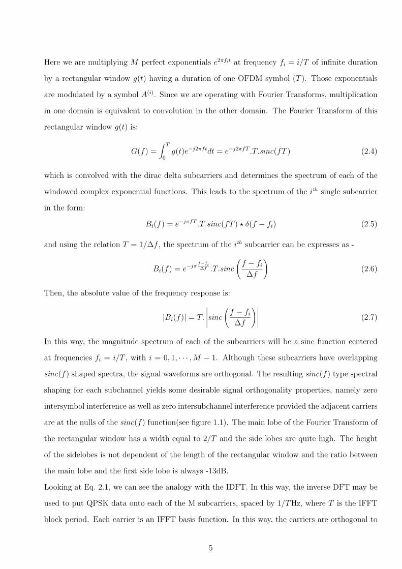
Here we are multiplying M perfect exponentials e2πfit at frequency fi = i/T of infinite duration

by a rectangular window g(t) having a duration of one OFDM symbol (T ). Those exponentials

are modulated by a symbol A(i). Since we are operating with Fourier Transforms, multiplication

in one domain is equivalent to convolution in the other domain. The Fourier Transform of this

rectangular window g(t) is:

G(f) =∫ T

0g(t)e−j2πftdt = e−j2πfT .T.sinc(fT ) (2.4)

which is convolved with the dirac delta subcarriers and determines the spectrum of each of the

windowed complex exponential functions. This leads to the spectrum of the ith single subcarrier

in the form:

Bi(f) = e−jπfT .T.sinc(fT ) ? δ(f − fi) (2.5)

and using the relation T = 1/∆f , the spectrum of the ith subcarrier can be expresses as -

Bi(f) = e−jπf−fi∆f .T.sinc

(f − fi

∆f

)(2.6)

Then, the absolute value of the frequency response is:

|Bi(f)| = T.

∣∣∣∣∣sinc

(f − fi

∆f

)∣∣∣∣∣ (2.7)

In this way, the magnitude spectrum of each of the subcarriers will be a sinc function centered

at frequencies fi = i/T , with i = 0, 1, · · · , M − 1. Although these subcarriers have overlapping

sinc(f) shaped spectra, the signal waveforms are orthogonal. The resulting sinc(f) type spectral

shaping for each subchannel yields some desirable signal orthogonality properties, namely zero

intersymbol interference as well as zero intersubchannel interference provided the adjacent carriers

are at the nulls of the sinc(f) function(see figure 1.1). The main lobe of the Fourier Transform of

the rectangular window has a width equal to 2/T and the side lobes are quite high. The height

of the sidelobes is not dependent of the length of the rectangular window and the ratio between

the main lobe and the first side lobe is always -13dB.

Looking at Eq. 2.1, we can see the analogy with the IDFT. In this way, the inverse DFT may be

used to put QPSK data onto each of the M subcarriers, spaced by 1/THz, where T is the IFFT

block period. Each carrier is an IFFT basis function. In this way, the carriers are orthogonal to

5

each other and may be demodulated by an equivalent FFT process without mutual interference

at the receiver.

Basically, the OFDM/DMT spectrum fulfills Nyquist’s criterion for an intersymbol interference

free pulse shape, which is present in the frequency domain and not in the time domain. Therefore,

instead of intersymbol interference(ISI), it is intercarrier interference(ICI) that is avoided by

having the maximum of one subcarrier spectrum corresponding to the zero crossing of all the

others.

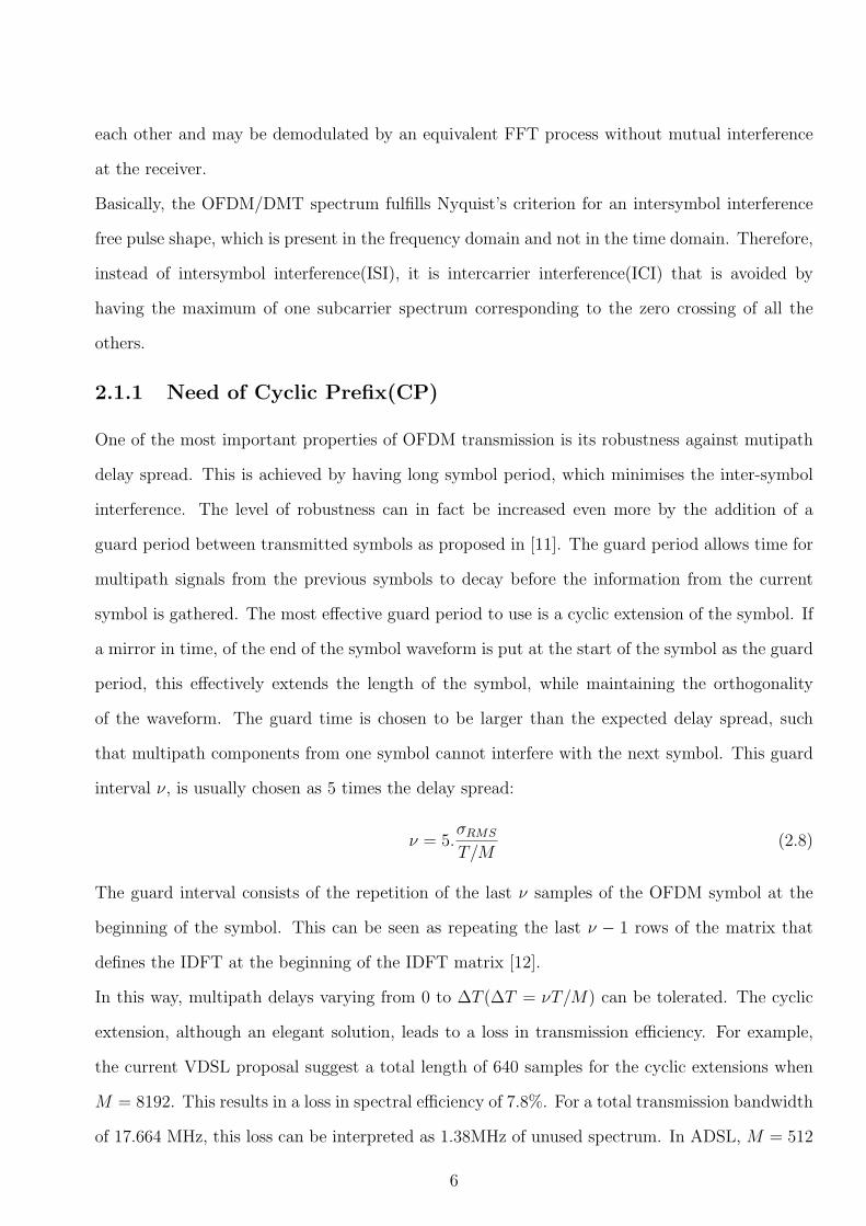
2.1.1 Need of Cyclic Prefix(CP)

One of the most important properties of OFDM transmission is its robustness against mutipath

delay spread. This is achieved by having long symbol period, which minimises the inter-symbol

interference. The level of robustness can in fact be increased even more by the addition of a

guard period between transmitted symbols as proposed in [11]. The guard period allows time for

multipath signals from the previous symbols to decay before the information from the current

symbol is gathered. The most effective guard period to use is a cyclic extension of the symbol. If

a mirror in time, of the end of the symbol waveform is put at the start of the symbol as the guard

period, this effectively extends the length of the symbol, while maintaining the orthogonality

of the waveform. The guard time is chosen to be larger than the expected delay spread, such

that multipath components from one symbol cannot interfere with the next symbol. This guard

interval ν, is usually chosen as 5 times the delay spread:

ν = 5.σRMS

T/M(2.8)

The guard interval consists of the repetition of the last ν samples of the OFDM symbol at the

beginning of the symbol. This can be seen as repeating the last ν − 1 rows of the matrix that

defines the IDFT at the beginning of the IDFT matrix [12].

In this way, multipath delays varying from 0 to ∆T (∆T = νT/M) can be tolerated. The cyclic

extension, although an elegant solution, leads to a loss in transmission efficiency. For example,

the current VDSL proposal suggest a total length of 640 samples for the cyclic extensions when

M = 8192. This results in a loss in spectral efficiency of 7.8%. For a total transmission bandwidth

of 17.664 MHz, this loss can be interpreted as 1.38MHz of unused spectrum. In ADSL, M = 512

6

Figure 2.1: OFDM Communication System

and the cyclic extension is 32 samples so the loss of efficiency is 6.25% [13]. In a DAB system,

this loss is 25% [14] and in HIPERLAN/2, 16 cyclic samples are added to the 64 data samples or

equaivalently, a loss in efficiency of 20% [15].

2.1.2 OFDM generation

Figure 2.1 shows a typical OFDM based communication system. To generate the OFDM signal,

the incoming serial data is first converted from serial to parallel and grouped into x bits each to

form a complex symbol (e.g. QPSK). The complex symbols are modulated in a baseband fashion

by the IDFT and converted back to serial data for transmission. A guard interval is inserted

between symbols to avoid intersymbol interference (ISI). The discrete symbols are converted to

analog and lowpass filtered before RF up-conversion. Then data stream is fed into the channel.

The receiver performs the inverse process of the transmitter. A one tap equalizer is used on each

subchannel to correct channel distortion. The tap coefficients of the filter q(i) are calculated based

on channel information [16].

Finally the data from the QPSK decoders is multiplexed back into a single serial data stream

which is passed on to the error correction decoder. This can correct errors which typically occur

when multipath causes selective fading of some carriers.

2.1.3 Virtual Carriers

Apart from the inefficiency of the cyclic prefix, another problem with OFDM is that it needs

Virtual Carriers(VC). Looking at the frequency response for one of the subchannels, we see that

it has high side lobes in adjacent channels that will be distorted by the DAC filter. Thus,

7

VCs are inserted into the roll off region of the DAC interpolation filter, i.e. null symbols are

transmitted to limit distortion, which further reduces transmission efficiency [17]. As we will see,

FMT needs fewer virtual carriers so it improves the total throughput. In HIPERLAN/2, 12 out

of 64 subcarriers are used as VCs which leads to an inefficiency of 18.75% [15].

2.1.4 Performance with Frequency and Timing Errors

The performance of the synchronization subsystem, in particular, the accuracy of frequency and

timing estimation, is a major influence on the overall OFDM system performance due to the over-

lapping subchannel spectra. For a single carrier system, these inaccuracies only give degradation

in the received SNR, rather than introducing interference.

Effects of Frequency Shift on OFDM

Carrier frequency errors which are caused by the mismatch between the oscillator in the trans-

mitter and in the receiver, result in a shift of the received signal’s spectrum in the frequency

domain. If the frequency error is an integer multiple I of the subcarrier spacing ∆f , then the

received frequency domain subcarriers are shifted by I.∆f . The subcarriers are still mutually

orthogonal, but the received data symbols, which were mapped to the OFDM spectrum, are in

the wrong position in the demodulated spectrum, resulting in a BER of 0.5.

If the carrier frequency error is not an integer multiple of the subcarrier spacing, then energy

spills over between the subcarriers, resulting in loss of their mutual orthogonality, In other words,

interference is observed between the subcarriers, which degrades the BER of the system.

If δf is the frequency offset, the total amount of ICI experienced by subcarrier i is the sum of the

interference amplitude contributions of all the other subcarriers in the OFDM symbol

Ii =∑j,j 6=i

Aj.Bj(fi + δf) (2.9)

The effects of Oscillator Phase Noise

A practical oscillator does not produce a carrier at exactly one frequency, but rather a carrier

that is phase modulated by random phase jitter [18]. As a result, the instantaneous frequency,

which is the time derivative of the phase, is never perfectly constant causing ICI in the OFDM

8

receiver. This becomes a particularly grave problem for systems operating above 25GHz since at

these frequencies it is difficult to find accurate and stable yet inexpensive oscillators.

Peak to Average Power Ratio

An OFDM signal is the sum of many subcarrier signals that are modulated independently by dif-

ferent modulation symbols. Therefore, they can give a large peak to average power ratio (PAPR)

when added coherently. Therefore, RF power amplifiers should be operated in a large linear

operating region, otherwise, the signal peaks get into the nonlinear region of the power amplifier

causing signal distortion. This distortion introduces intermodulation among the subcarriers and

also out of band radiation [10]

2.2 Reason to introduce FMT

Based on this overview we will highlight the main problems in OFDM that FMT will address.

Cyclic Prefix:

The cyclic extension, although an elegant solution, leads to a loss in transmission efficiency. For

instance, HIPERLAN/2 uses 16 samples out of 80 for the cyclic prefix, which leads to a loss in

bandwidth efficiency of 20%.

Virtual carriers:

Since the sidelobes of the OFDM signal are high (the first sidelobe of a sinc signal is only 13dB

lower than the main lobe, independent of the number of subcarriers), there is significant power

leaking into adjacent bands. In order to reduce interference into adjacent bands, a number of

subcarriers at the dge of the multiplex are not used. These virtual carriers are also introduced

because the low pass filter following the Digital to Analogue Conversor will distort the subcarriers

close to the pass band edges. In HIPERLAN/2, 12 out of 64 subcarriers are virtual carriers which

is 18.75% of the total number of subcarriers. Due to he high spectral containment of FMT, it

needs fewer virtual carriers which will provide a higher data throughput.

Although FMT modulation goes someway to addressing the highlighted problems, it comes at

the expense of higher computational complexity.

9

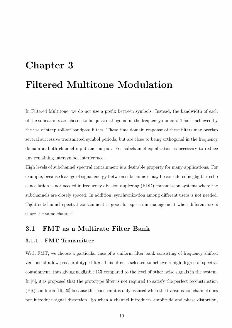
Chapter 3

Filtered Multitone Modulation

In Filtered Multitone, we do not use a prefix between symbols. Instead, the bandwidth of each

of the subcarriers are chosen to be quasi orthogonal in the frequency domain. This is achieved by

the use of steep roll-off bandpass filters. These time domain response of these filters may overlap

several successive transmitted symbol periods, but are close to being orthogonal in the frequency

domain at both channel input and output. Per subchannel equalization is necessary to reduce

any remaining intersymbol interference.

High levels of subchannel spectral containment is a desirable property for many applications. For

example, because leakage of signal energy between subchannels may be considered negligible, echo

cancellation is not needed in frequency division duplexing (FDD) transmission systems where the

subchannels are closely spaced. In addition, synchronization among different users is not needed.

Tight subchannel spectral containment is good for spectrum management when different users

share the same channel.

3.1 FMT as a Multirate Filter Bank

3.1.1 FMT Transmitter

With FMT, we choose a particular case of a uniform filter bank consisting of frequency shifted

versions of a low pass prototype filter. This filter is selected to achieve a high degree of spectral

containment, thus giving negligible ICI compared to the level of other noise signals in the system.

In [6], it is proposed that the prototype filter is not required to satisfy the perfect reconstruction

(PR) condition [19, 20] because this constraint is only assured when the transmission channel does

not introduce signal distortion. So when a channel introduces amplitude and phase distortion,

10

the objective of high spectral containment is more easily achieved if the perfect reconstruction

constraint is relaxed although we will need to use equalization to remove ISI.

We can use any of the well known methods (e.g. Window, Remez, etc [21]) to design the lowpass

prototype filter h(n) with the objective of obtaining a symmetric Finite Impulse Response(FIR)

filter with real coefficients that would approximate the ideal frequency response H(f) shown in

figure 3.1.

Figure 3.1: Ideal Frequency Response of the low pass prototype

With FMT, orthogonality between subchannels is ensured by using non-overlapping spectral char-

acteristics as compared with the overlapping sinc(f) type spectra employed in OFDM. Since the

linear transmission medium does not destroy orthogonality achieved in this manner, cyclic pre-

fixing is not needed. Clearly, the required amount of spectral containment must be achieved with

acceptable filtering complexity. In a critically sampled filter bank [20], the frequency separation

of the pass bands will be 1/T with a total of M bands. In this way, each of the transmitter pass

band filters will be frequency-shifted versions of the low pass filter as shown in figure 3.2:

Figure 3.2: Frequency shifted version of the prototype

h(i)(n) =1√M

h(n).ej2π iM

n, n = 0, 1, · · · , Mγ − 1, and i = 0, 1, · · · , M − 1 (3.1)

The length of the prototype filter Mγ is a multiple of the number of subchannels M . Parameter

γ is called the overlap [20, 7] since it is the number of blocks (each of M samples) to which the

prototype is expanded. Usual values for γ in FMT are between 8 and 20. In figure 1.2 we show

the frequency response of the first 6 subchannels of a 64 subchannel system using a prototype

with overlap γ = 14. Since the out of band power is lower than 55dB in adjacent bands and even

11

less for other bands, we can consider that the ICI is zero compared with other noise signals in

the system such as AWGN.

The direct implementation of the FMT filter bank(both transmitter and receiver) is shown in

figure 3.3. The inputs are QAM or QPSK symbols not necessarily from the same constellation.

After upsampling by a factor of M (see [21]), each modulation symbol is filtered at a rate M/T

(where T is the FMT symbol period) by the subchannel filter defined in Eq. 3.1 centred at

frequency fi = i/T . The transmit signal x(n) is obtained at the transmission rate M/T by

adding together the M filter output signals that have been appropriately frequency shifted.

Figure 3.3: Direct implementation of FMT system

In the notation and figures, we have denoted k as the index for samples with a sampling period

equal to T and n for the samples with a sampling period equal to T/M . The system shown

in Figure 3.3 would not be practical if we could not derive an efficient implementation since all

the filtering operations are performed in parallel and at a rate M/T . We will now see how to

derive from figure 3.3, an efficient implementation that makes use of the Inverse Discrete Fourier

Transform (IDFT).

When analysing multirate signal processing systems we usually arrive at the situation where filter

responses are better described in terms of their polyphase components [20].

If we take the prototype h(n) with Z transform

H(z) =∞∑

n=−∞h(n)z−n (3.2)

we can always partition the index n into M phases, where each phase is characterized by choosing

12

indices which are identical modulo M . Then for any integer M , we can decompose H(z) as:

H(z) =∞∑

n=−∞h(nM)z−nM + z−1

∞∑n=−∞

h(nM + 1)z−nM + · · ·+ z−(M−1)∞∑

n=−∞h(nM + M − 1)z−nM

(3.3)

Thus, the kth phase of h(n) is defined by:

h(k)(m) = h(mM + k) (3.4)

We now apply the polyphase representation to show how the computationally efficient implemen-

tation can be applied to the structure of trasmitter section of the figure 3.3.

Using the filter definition from Eq. 3.1, the signal at the channel input in figure 3.3 is given by:

x(n) =1√M

M−1∑i=0

∞∑k=−∞

A(i)(k)h(n− kM)ej2πi(n−kM)/M (3.5)

x(n) =∞∑

k=−∞h(n− kM)

1√M

M−1∑i=0

A(i)(k)ej2πin/M (3.6)

A change of notation n = lM +m allows us to introduce the polyphase components of h(n). With

the notations x(lM + m) = x(m)(l) and h(lM + m) = h(m)(l) for m = 0, 1, · · · , M − 1, we obtain:

x(m)(l) =∞∑

k=−∞h(m)(l − k)

{1√M

M−1∑i=0

A(i)(k)ej2πim/M

}(3.7)

x(m)(l) =∞∑

k=−∞h(m)(l − k)a(m)(k) (3.8)

where a(m)(k), 0 ≤ m ≤ M − 1, is the IDFT of A(i)(k) that may be efficiently implemented with

the Inverse Fast Fourier Transform (IFFT). The mth output of the IFFT is filtered by the mth

polyphase component of h(n) and this filtering operation is performed at rate 1/T and not M/T .

From Eq. 3.7 we can derive the efficient implementation shown in Figure 3.4.

We can see in figure 3.4 that the filtering operation is performed at rate 1/T instead of M/T . At

each instant, only the output of one polyphase filter needs to be computed due to the Parallel to

Serial (P/S) and not the entire M samples as required in figure 3.3.

3.1.2 FMT Receiver

In the receiver filter bank architecture shown in figure 3.3, the receiving filters {g(i)(n)} are

designed to be matched to the corresponding ones in the transmitter, i.e. from Eq. 3.1 Gi(f) =

13

Figure 3.4: FMT Transmitter: Efficient Implementation

(H(i)(f))∗. Using the property of DTFT (H(i)(f))∗F−1

−→ (h(i)(−n))∗, let -

g′(i)(n) = (h(i)(−n))∗ (3.9)

therefore:

g′(i)(n) =1√M

h(−n).e−j 2πM

(−n)i, n = −Mγ + 1, · · · , 0, (3.10)

However, this filter is not causal. Since g(n) is defined for n = −Mγ + 1, · · · ,−1, 0 we need to

apply a minimum delay of Mγ− 1 samples to make it causal. However, differently to some other

publications eg [22], we will apply a delay which is a multiple of the block size M. Specifically, we

delay it by Mγ samples and we call this response g(i)(n). This sample delay difference compared

with other publications is what will allow us to define the efficient implementation. We should

note that since we are using multirate blocks, this difference of one sample makes a change to the

overall response of the filter. In the efficient implementation, it will also allow us to take blocks

of M samples in a different way, otherwise, there will be an offset in the way we take the blocks

of samples in the transmitter and in the receiver. Applying a delay of Mγ samples to Eq. 3.10,

the matched filter will maximize the SNR at that specific instant [1]. Therefore, the system will

have an overall delay of γ blocks. However, since the prototype was not designed with the perfect

reconstruction constraint, we cannot say that the output of the filter bank is A(k − γ).

Applying the delay to the receiver filters in Eq. 3.10 we obtain:

g(i)(n) = g′(i)(n−Mγ) (3.11)

g(i)(n) =1√M

h(−(n−Mγ)).ej 2πM

(n−Mγ)i, n = 1, 2, · · · , Mγ (3.12)

14

which simplifies to:

g(i)(n) =1√M

h(Mγ − n).ej 2πM

ni, n = 1, 2, · · · , Mγ (3.13)

and since h(n) is symmetric, then the receiver filter at the ith subchannel is:

g(i)(n) =1√M

h(n− 1).ej 2πM

ni, n = 1, 2, · · · , Mγ (3.14)

Applying Eq. 3.12, at the output of the ith subchannel in figure 3.3 we get:

B(i)(k) =Mγ∑n=1

y(kM − n)g(i)(n) =1√M

Mγ∑n=1

y(kM − n)h(n− 1).ej 2πM

ni, (3.15)

To introduce the polyphase components of h(n) defined in Eq. 3.4 we decompose n as n =

lM + t, l = 0, 1, · · · , γ − 1 and t = 1, 2, · · · , M to yield,

B(i)(k) =1√M

M∑t=1

γ−1∑l=0

y(kM − lM − t)h(lM + t− 1).ej 2πM

(lM+t)i (3.16)

=1√M

M∑t=1

γ−1∑l=0

y((k − l)M − t)h(lM + t− 1).ej 2πM

ti (3.17)

If we make a change of variable p = t− 1:

B(i)(k) =1√M

M−1∑p=0

γ−1∑l=0

y((k − l)M − (p + 1))h(lM + p).ej 2πM

(p+1)i (3.18)

and applying:

ej 2πM

(p+1)i = e−j 2πM

(M−p−1)i (3.19)

we obtain:

B(i)(k) =1√M

M−1∑p=0

γ−1∑l=0

y((k − l)M − p− 1)h(lM + p)

.e−j 2πM

(M−p−1)i (3.20)

From Eq. 3.20 we are able to derive the efficient implementation shown in figure 3.5 where we

apply the DFT operation (efficiently implemented with the FFT) to the M outputs of the M

polyphase filters.

We can also see from Eq. 3.20 that the implementation in figure 3.5 is mirrored (matched) to the

implementation in figure 3.4. Since the prototype is symmetric and has Mγ samples, for each

of the polyphase components h(i)(n) = h(nM + i), the matched filter is actually h(M−i−1)(n).

That is why they are in reverse order to the ones in figure 3.4, since the whole implementation is

matched to that of figure 3.4.

15

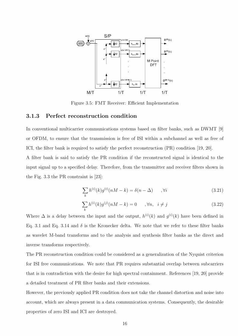
Figure 3.5: FMT Receiver: Efficient Implementation

3.1.3 Perfect reconstruction condition

In conventional multicarrier communications systems based on filter banks, such as DWMT [9]

or OFDM, to ensure that the transmission is free of ISI within a subchannel as well as free of

ICI, the filter bank is required to satisfy the perfect reconstruction (PR) condition [19, 20].

A filter bank is said to satisfy the PR condition if the reconstructed signal is identical to the

input signal up to a specified delay. Therefore, from the transmitter and receiver filters shown in

the Fig. 3.3 the PR constraint is [23]:

∑k

h(i)(k)g(i)(nM − k) = δ(n−∆) ,∀i (3.21)

∑k

h(i)(k)g(j)(nM − k) = 0 ,∀n, i 6= j (3.22)

Where ∆ is a delay between the input and the output, h(i)(k) and g(i)(k) have been defined in

Eq. 3.1 and Eq. 3.14 and δ is the Kronecker delta. We note that we refer to these filter banks

as wavelet M-band transforms and to the analysis and synthesis filter banks as the direct and

inverse transforms respectively.

The PR reconstruction condition could be considered as a generalization of the Nyquist criterion

for ISI free communications. We note that PR requires substantial overlap between subcarriers

that is in contradiction with the desire for high spectral containment. References [19, 20] provide

a detailed treatment of PR filter banks and their extensions.

However, the previously applied PR condition does not take the channel distortion and noise into

account, which are always present in a data communication systems. Consequently, the desirable

properties of zero ISI and ICI are destroyed.

16

The approach followed in FMT is to remove ICI almost completely irrespective of the channel

and then to remove the remaining ISI per subchannel using equalization. Therefore, by relaxing

the PR constraints and introducing signal equalization at the receiver, filters that achieve high

spectral containment can be found. In the FMT filter bank, the design criterion will be high

spectral containment. High spectral containment will avoid ICI but ISI will now exist in each

subchannel and it will need to be removed.

We note that only a perfect brick wall filter would achieve PR and also satisfy the previously

outlined FMT principles. Unfortunately this filter is not practical since it would require an

infinitely long prototype filter.

3.1.4 Prototype Design

In FMT modulation, the prototype filter completely defines the system. The choice of the pro-

totype filter for the realization of the polyphase filter bank allows various tradeoffs between the

number of subchannels, the level of spectral containment, the complexity of implementation and

signal latency to be made. These tradeoffs are possible because the number of subchannels can be

reduced without incurring a transmission efficiency loss, whereas in OFDM the minimum number

of subchannels is constrained by efficiency requirements owing to the use of the cyclic prefix.

Since we are not required to design a prototype based on the PR constraint, we will focus on

prototypes that accomplish high levels of spectral containment with the minimum complexity.

This prototype filter approximates an ideal filter which has a frequency response equal to zero

outside the interval |f | ≤ 12T

Hz as shown in figure 3.1. In the design of the low pass filter h(n),

the sampling rate will be the highest system rate i.e., M/T . Therefore, the digital frequency (at

sampling rate M/T ) limit will be 1/(2M) (see figure 3.1). We will approximate this response with

a linear phase FIR prototype filter with Mγ real coefficients. In this way, each of the polyphase

filters will be a filter with real coefficients and length γ. We also note that the prototype is

symmetric but that the polyphase components are not.

17

3.2 OFDM as a filter bank

We can view conventional OFDM modulation from the same point of view as FMT. In this

situation, the low pass prototype is a rectangular pulse in the time domain i.e. a sinc function

in the frequency domain. The length of the overlap in this case will be γ = 1. As we have seen

in the previous section, the higher the overlap, the higher the spectral containment. This is the

reason that we do not accomplish high spectral containment in OFDM. However, in this case the

prototype accomplishes perfect reconstruction.

Although all subchannels overlap in frequency, the system exhibits neither ISI nor ICI (PR con-

dition) as long as the channel is non dispersive, at the expense of high spectral overlap.

Figure 2.1 shows the block diagram of a OFDM/DMT system. All the filters depicted at the

output branches of the IDFT block have the trivial impulse response

h(i)(k) = δ(k), for i = 0, 1, · · · , M − 1 (3.23)

where h(i)(k) represents the ith polyphase components of a prototype filter h(n) with impulse

response:

h(n) = 1, for n = 0, 1, · · · , M − 1 (3.24)

When the prototype h(n) is an ideal rectangular pulse in time, the system will be called OFDM/DMT.

Alternatively, when h(n) is designed to minimize the overlap between the frequency response of

two adjacent subchannels(i.e., an ideal rectangular pulse in the frequency domain) the corre-

sponding system is called FMT.

18

Chapter 4

Equalization in FMT

Since in the prototype filter design we try to have all the spectra contained in 1/(2T ), the Nyquist

criterion will not be accomplished owing to the rapid decay of the frequency response before

f = 1/(2T ). The longer the overlap γ, the flatter can be the filter passband out to frequencies

close to f = 1/(2T ) and so less ISI will be introduced.

Figure 4.1: Equivalent subchannel

Assuming that the subchannels are well separated in frequency , the overall response for each of

the subchannels will be independent of the adjacent channels (no ICI) and it can be considered

equivalent to the cascade of the ith transmitter filter, the multipath channel, c(n), and the ith

receiver filter as shown in figure 4.1. This response will need to be equalized by a per subchannel

equalizer as shown in figure 4.2.

Figure 4.2: Per subchannel equalization

It is important to note that even without the effect of the channel and the additive noise, we

would still have ISI due to violation of the PR reconstruction condition. In figure 4.3, we show

19

the impulse response of the ith subchannel without the effect of the multipath channel. For an

overlap value γ, the length of the equivalent channel has (2γ − 1) samples.

Figure 4.3: Equivalent impulse response of ith subchannel, γ = 14, FIR prototype: Hamming,fc = 0.38/T

4.1 Conventional Equalizers:

Linear equalizer and Decision Feedback equalizer(DFE) are well established and effective ap-

proaches for the mitigation of the ISI effects(see figures 4.4 and 4.5 respectively).

Figure 4.4: Linear equalizer for FMT(overlap=γ)

Figure 4.5: Differential Feedback Equalizer(DFE) for FMT(overlap=γ)

20

Here no of taps are chosen on the basis of overall subchannel impulse response. Two optimality

criteria have been used to optimize the coefficients of DFE filters, namely the Zero Forcing (ZF)

criterion and the Minimum Mean Square Error(MMSE) criterion.

4.1.1 Computation of the MMSE equalizer coefficients based on chan-nel estimation

DFE equalizer

Here equalizer is used at the output of each of the subchannels. In the equalizer, the input B(i)(k),

the desired output, A(i)(k) and the filter tap weights are all assumed to be complex variables.

The estimated error e(i)(k) at the decision device is also complex and we may write :

e(i)(k) = d(i)(k)− y(i)(k) (4.1)

where d(i)(k) is the output of the slicer and y(i)(k) the output of filtering operation. The MMSE

criterion to compute the tap coeficients will minimize:

E|e(i)(k)|2 = E|d(i)(k)− y(i)(k)|2 (4.2)

Here we consider a DFE with γ feedforward tap coefficients and γ − 1 feedback tap coefficients.

Then it is mathematically convenient to define an augmented response vector for the DFE as:

wi = [w∗FF,i(0), w∗

FF,i(1), · · · , w∗FF,i(γ − 1),−w∗

FB,i(1),−w∗FB,i(2), · · · ,−w∗

FB,i(γ − 1)]T (4.3)

and the corresponding augmented DFE input vector x(i)(k):

x(i)(k) = [B(i)(k), B(i)(k−1), · · · , B(i)(k−γ +1), d(i)(k−1), d(i)(k−2), · · · , d(i)(k−γ +1)]T (4.4)

where B(i)(k) is the output of multirate filter bank:

B(i)(k) =Neq−1∑n=0

h(i)eq (n)A(i)(k − n) + n(i)

r (k) (4.5)

where h(i)eq is the overall response of the ith subchannel. With ideal channel it is -

h(i)eq (k) =

(g(i)(n) ? h(i)(n)

)↓M

(4.6)

Therefore the output of the DFE operation is -

y(i)(k) = wHi x(i)(k) (4.7)

21

We now assume that the decisions are correct, d(i)(k) = A(i)(k−2γ +1). Thus data in the tapped

delay line becomes:

x(i)(k) = [B(i)(k), B(i)(k−1), · · · , B(i)(k−γ+1), A(i)(k−2γ), A(i)(k−2γ−1), · · · , A(i)(k−3γ+2)]T

(4.8)

The MMSE for the MMSE-DFE is [24]:

σ2MMSE−DFE,i = min

wi

E{|d(i)(k)− y(i)(k)|2

}(4.9)

When the filter taps are set to the optimal values, the principle of orthogonality for the complex

case [25] gives -

E{e(i)∗

o (k)x(i)(k − p)} = 0, for p = 0, 1, · · · , 2γ − 2 (4.10)

Where e(i)o is the optimum estimation error computed with the optimum Wiener-Hopf taps (wo,i):

e(i)o (k) = A(i)(k − 2γ + 1)− wH

o,ix(i)(k) (4.11)

e(i)∗

o (k) = A(i)∗(k − 2γ + 1)− x(i)H

(k)wo,i (4.12)

From above equations, the orthogonality defined in Eq. 4.10 can be packed together as:

Ee(i)∗

o (k).x(i)(k) = E{[

A(i)∗(k − 2γ + 1)− x(i)H

(k)wo,i

]x(i)(k)

}= [0, 0, · · · , 0]T (4.13)

Solving above equation, the Wiener-Hopf optimal coefficients are:

wo,i =(R(i)

xx

)−1p(i) (4.14)

where:

p(i) = E{A(i)∗(k − 2γ + 1)x(i)(k)

}=

σ2A(i)heq,i(2γ − 1)

σ2A(i)heq,i(2γ − 2)

· · ·σ2

A(i)heq,i(γ)0· · ·0

(2γ−1)×1

(4.15)

and

(4.16)

where we have applied:

22

• noise uncorrelated with the data

• data input, A(i)(k), are independent at different sampling times and variance σ2A(i)

and the autocorrelation function R(i)xx

in Eq. 4.29 is defined as:

R(i)xx

= E{x(i)(k)x(i)H

(k)}

(4.17)

Since the noise is uncorrelated with the data, we can represent the autocorrelation matrix Rxx as

the addition of two matrices, one depending on the data and the other depending on the noise.

Rxx = Rxxdata + Rxxnoise (4.18)

We now divide the matrix Rxxdata into four different matrix blocks:

Aγ×γ, B(γ−1)×(γ−1), Cγ×(γ−1), D(γ−1)×γ (4.19)

Rxxdata =

[A CD B

](2γ−1)×(2γ−1)

(4.20)

These matrices are defined as:

[A]i,j = σ2A

Neq−1∑t=0

heq(t)h∗eq(t + i− j) i, j = 1, 2, · · · , γ (4.21)

[B]i,j = σ2Aδ(i− j) i, j = 1, 2, · · · , γ − 1 (4.22)

[C]i,j = heq(2γ + j − i)σ2A i = 1, 2, · · · , γ, j = 1, 2, · · · , γ − 1 (4.23)

[D]j,i = [C]∗i,j j = 1, 2, · · · , γ − 1, i = 1, 2, · · · , γ (4.24)

In Rxxnoise, since the data is uncorrelated with the noise, the only elements nonzero will be a

block matrix Eγ×γ

Rxxnoise =

[E 00 0

](2γ−1)×(2γ−1)

(4.25)

[E]i,j = σ2n

Mγ∑n1=1

g(i)(n1).g(i)∗(n1 + i− j) (4.26)

where σ2n is noise variance.

23

Linear Equalizer:

In linear equalizer augmented response vector is:

wi = [w(i)∗(0), w(i)∗(1), · · · , w(i)∗(2γ − 2)]T (4.27)

and LE input vector x(i)(k):

x(i)(k) = [B(i)(k), B(i)(k − 1), · · · , B(i)(k − 2γ + 2)]T (4.28)

Solving in the same way as DFE, the Wiener-Hopf optimal coefficients for LE are:

wo,i =(R(i)

xx

)−1p(i) (4.29)

where:

p(i) =

σ2

A(i)heq,i(2γ − 1)σ2

A(i)heq,i(2γ − 2)σ2

A(i)heq,i(2γ − 3)· · ·

σ2A(i)heq,i(1)

(2γ−1)×1

(4.30)

and

Rxx = Rxxdata + Rxxnoise (4.31)

all are of dimension (2γ − 1)× (2γ − 1)

[Rxxdata]i,j = σ2A

Neq−1∑t=0

heq(t)h∗eq(t + i− j) i, j = 1, 2, · · · , (2γ − 1) (4.32)

and

[Rxxnoise]i,j = σ2n

Mγ∑n1=1

g(i)(n1).g(i)∗(n1 + i− j) (4.33)

4.1.2 Simulation Results with DFE and Linear equalizers

Simulation is performed on uniformly distributed constellation symbols and MMSE-LE, MMSE-

DFE equalizers are used. Results without TCM and with Ungerboek-based TCM are shown in

figures 4.6 and 4.7 respectively. Here for FMT MMSE-DFE based equalizer gives slightly better

results than MMSE-LE.

24

Figure 4.6: Results without TCM(M=64, γ = 14, FIR prototype: Hamming fc = 0.38/T )

Figure 4.7: Results with TCM(M=64, γ = 14, FIR prototype: Hamming fc = 0.38/T )

25

4.2 Turbo Equalizer

The process of making hard decisions on the channel symbols actually destroys information per-

taining to how likely each of the possible channel symbols might have been, however. This

additional ”soft” information can be converted into probabilities that each of the received code

word bits takes on the value of zero or one that, after deinterleaving, is precisely the form of infor-

mation that can be exploited by a BER optimal decoding algorithm. Many practical systems use

this form of soft-input error control decoding by passing soft information between an equalizer

and decoding algorithm.

The remarkable performance of turbo codes makes it clear that the soft information need not only

flow in one direction. Once the error control decoding algorithm processes the soft information

it can, in turn, generate its own soft information indicating the relative likelihood of each of the

transmitted bits. This soft information from the decoder could then be properly interleaved and

taken into account in the equalization process, creating a feedback loop between the equalizer

and decoder, through which each of the constituent algorithms communicates its belief about the

relative likelihood that each given bits takes on a particular value. This process is often termed

”belief propagation” or ”message passing” and has a number of important connections to methods

in artificial intelligence, statistical inference, and graphical learning theory. The feedback loop

structure for bidirectional flow of soft information is essentially the process of turbo equalization.

When processing soft information as an input to the equalizer or decoder, it is assumed that

the soft information about each bit (or channel symbol) is an independent piece of information.

This enables simple, fast algorithms to be used for each of the equalizer and decoder. If the

decoder formulates its soft information about a given bit, based on soft information provided

to it from the equalizer about exactly the same bit, then the equalizer can not consider this

information to be independent of its channel observations. In effect, this would create a feedback

loop in the overall process of length two: the equalizer informs the decoder about a given bit,

and then the decoder simply reinforms the equalizer what it already knows. To avoid such short

cycles in the feedback and in hopes of avoiding local minima and limit cycle behaviour in the

process, when soft information is passed between constituent algorithms, such information is never

formed based on the information passed into the algorithm concerning the same bit. Basically,

26

this amounts to the equalizer only telling the decoder new information about a given bit based

on information it gathered from distant parts of the received signal. Similarly, the decoder only

tells the equalizer information it gathered from distant parts of the encoded bit stream. As a

result, the iterative equalization and decoding process can continue for many iterations before

cycles are introduced, which eventually limits further improvements. This process of only passing

”extrinsic information” between constituent decoders is essential to the performance of turbo

decoding algorithms.

In all these systems, maximum a posteriori (MAP) based techniques, most often a Viterbi Al-

gorithm(VA) producing soft output information, are used exclusively for both equalization and

decoding [26, 27]. The more complex BCJR algorithm [28] were implemented in [27].

The MAP/ML-based solutions often suffer from high computational load for channels with long

memory or large constellation sizes(expensive equalizer) or convolutional codes with long mem-

ory(expensive decoder). This situation is exacerbated by the need to perform equalization and

decoding several times for each block of data. Recently, reduced complexity structure of soft-in

soft-out (SISO) equalizers were introduced using linear equalizer(LE) and DFE based on MMSE

criteria[29, 30]. The MAP equalizer is thus replaced with an LE or DFE, whose filter parameters

are updated for every output symbol of the equalizer.

To overcome the problems of the conventional equalization schemes and to introduce more flexi-

bility to FMT system, we propose turbo equalization as a viable solution.

4.3 Proposed equalization scheme

Figure 4.8 depicts the basic system investigated. The (binary) data dj is encoded with a (binary)

convolutional encoder yielding code symbols xj, which are mapped to the alphabet B of the

signal constellation. Here, for simplicity we assume binary phase shift keying (BPSK), i.e., B ∈

{−1, +1}. The interleaver permutes the code symbols xj and outputs xn. This operation is

denoted by xn =∏

(xj), where∏

(.) is a fixed random interleaver. The permutation∏−1(.), the

de-interleaver, reverses the∏

(.) operation. The noise is modelled as additive white Gaussian

noise (AWGN) and independent of the data.

A turbo equalizer consists of a SISO Equalizer and a SISO decoder, operating in an iterative

27

Figure 4.8: Basic Turbo-FMT System

manner. The L-value operator L(x), called log likelihood ratio (LLR), is applied to quantities

x ∈ {−1, +1} and is given by

L(x) ≡ logP (x = +1)

P (x = −1)(4.34)

The equalizer inputs a priori L1(xn) LLR and outputs a posteriori LLR minus a priori LLR

called the extrinsic LLR LE(xn). For the initial equalization step, no a priori information is

available and hence we have L1(xn) = 0. The equalizer output after interleaving is considered

to be a priori LLR L2(xj) for the decoder. The decoder also computes extrinsic LLRs LD(xj)

which after de-interleaving is given to the equalizer as input. Note that L2(xj) =∏−1(LE(xn))

and L1(xn) =∏

(LD(xn)). The SISO decoder also computes the data bit estimates. A suitably

chosen termination criterion stops the iterative process. The resulting turbo equalization scheme

for FMT system is shown in figure 4.9.

Figure 4.9: Turbo FMT Equalizer

28

4.3.1 SISO equalizer

We have not shown the subcarrier dependence in many equations so as not to make them very

confusing. The signal model can be represented in a compact form as: zn = Hxn + wn, where

zn is the channel observation, xn is the transmitted signal, H is the channel convolution ma-

trix and wn is AWGN with variance σ2 = No/2 per dimension. The overall channel response,

(h(m)eq (k)), k = 0, 1, · · · , 2γ − 2 of the mth subchannel due to transmit and receive filters is inde-

pendent of subchannel index. Thus, the overall channel memory is µ = 2γ − 2.

h(m)eq =

1

M

Mγ−1∑m=0

h(n)h(kM − n− 1) (4.35)

We have considered both MMSE-LE and MMSE-DFE, as developed in [29, 30], for the SISO

equalization task. Since overall channel impulse response is designed to be real, therefore we will

have only real tap coefficients. In exact implementation, we will have time varying coefficients.

We can also use approximate implementation in which we use time invariant coefficients, thus

reducing computational complexity at slight performance loss.

4.3.2 SISO Decoder

For the decoding stage, we consider a binary rate-1/n convolutional code with constraint length k.

The BCJR decoding algorithm [28] is known to yield the optimal symbol estimate with minimum

symbol-error rate. The essential part is the BCJR algorithm’s ability to yield soft information in

the form of a posteriori LLRs for coded and information bits. Using the same notation as in [28],

for stage t of the code trellis transiting from state St−1 = s′ to St = s associated with input dt and

output xj = (x1t x

2t · · · , xn

t )(where {xj} ↔ {xkt } with j = (t− 1)n + k for a rate-1/n convolutional

code), we have

Λ(xkt ) = log

∑S+

k

αt−1(s′) γt(s

′, s) βt(s)

∑S−

k

αt−1(s′) γt(s

′, s) βt(s)(4.36)

29

where S+k is the set of pairs (s′, s) such that the kth coded bit at stage t is 1 and S−

k is corresponding

set for -1, and for information bit it is defined as

Λ(dt) = log

∑U+

k

αt−1(s′) γt(s

′, s) βt(s)

∑U−

k

αt−1(s′) γt(s

′, s) βt(s)(4.37)

where U+k is the set of pairs (s′, s) such that kth information bit at stage t is 1 and U−

k is

corresponding set for 0. The terms αt(s), βt(s) are defined with forward and backward recursion

as(τ denotes the frame length of information bits),

αt(s) =∑s′

αt−1(s′) γt(s

′, s), 1 ≤ t ≤ τ (4.38)

βt(s) =∑s′

βt+1(s′) γt+1(s, s

′), τ − 1 ≥ t ≥ 0 (4.39)

and γt(s′, s) denotes the transition probability for the branch s′ → s for the stage t of the code

trellisγt(s

′, s) = P (St = s|St−1 = s′) =∏n

l=1 P (xlt)

=∏n

l=112[1 + xl

t tanh(L2(xlt))]

(4.40)

So the extrinsic information produced by the decoder can be computed as

LD(xkt ) = log

∑S+

k

αt−1(s′)βt(s)

n∏l=1,l 6=k

P (xlt)

∑S−

k

αt−1(s′)βt(s)

n∏l=1,l 6=k

P (xlt)

= ΛD(xkt )− L2(x

kt )

(4.41)

where again {xj} ↔ {xkt } with j = (t − 1)n + k for a rate-1/n convolutional code. These after

interleaving are again passed to the SISO equalizer.

4.3.3 Simulation Results

Now, we evaluate the performance of our proposed turbo equalization based schemes. The channel

bandwidth is taken to be 20 MHz with 64 subcarrier frequency slots. BPSK modulation is used to

map the bitstream into an information symbol sequence. The sampling rate is 20 Msamples/sec.

FMT symbol duration (T) is taken as 3.2 s to achieve spectral efficiency of 1 bit/sec/Hz (for

uncoded system). We assume the channel is known only to the receiver through the use of pilot

30

Figure 4.10: BER performance for MMSE-DFE

Figure 4.11: BER performance for MMSE-LE

tones. We have used Hamming window with cutoff frequency, fcutoff = 0.315/T . The overlap

factor γ is 10. The simulations have been performed on 2000 FMT blocks of length 64 each. We

took a perfectly terminated rate-1/2 convolutional encoder having the generator polynomial G =

[7 5]. The length of the equalizer filter was 36. A random interleaver of length 640 was taken. In

figure 4.10 and 4.11 we show the BER performance as a function of SNR for the turbo equalization

based scheme using MMSE-DFE and MMSE-LE, respectively. We performed 8 iterations for each

scheme.

For the first iteration the performance of MMSE-DFE is much better than MMSE-LE as ex-

31

pected. In the absence of any a priori information, MMSE-DFE which uses non-linear equalizer

outperforms it’s linear counterpart MMSE-LE except at low SNR (0-5 dB). Over the subsequent

iterations (from 2 to 8), we see that the performance of MMSE-LE improves substantially com-

pared to MMSE-DFE. This can be explained from the fact that DFE uses a slicer in the feedback

loop. This hard limiting destroys the soft information in the received signal. On the other hand,

LE maintains the fidelity of soft information with iterations and thus gives impressive gains. Thus,

MMSE-LE achieves a gain of 2.37 dB against MMSE-DFE at BER = 10-4 after 8 iterations. We

attained convergence by fifth iteration in both schemes.

32

Chapter 5

Conclusion and Future scope

5.1 Conclusion

• In this report we presented the theory of FMT modulation and detailed its advantages

and limitations when used in wireless environments. We have seen, that at the expense

of higher computational complexity and better spectral containment, we obtain a higher

spectral efficiency than conventional OFDM.

• Multiple Access Filtered Multitone(MA-FMT) in the uplink is potentially attractive for

future wireless access. The interesting thing about FMT is that since the ICI is negligible,

it is a good option for spectrum management in which we assign different subcarriers to

different users. In this way, we can allocate different users in different subchannels without

need for frame synchronization among different users.

• Broadband Fixed Wireless Access in which there is a long delay spread and the need for

a long CP results in a loss of efficiency in conventional OFDM. In addition, since the

transmitter and receiver are not mobile, the multipath channel is more static than other

wireless systems(e.g. mobile phone networks), therefore training sequences to initialize the

channel equalizer do not need to be sent as often.

• We obtained very impressive gains by using turbo equalization based schemes in FMT

system at the cost of increased computational complexity. However, we can use approximate

implementation to bring down complexity at slight performance loss. The complexity of the

system is mainly due to iterations and we obtain impressive gain with iterations. Thus, we

obtained a simple-to-design system providing excellent tradeoff between performance and

33

complexity. Therefore, it may be a valid alternative to OFDM in wireless applications.

5.2 Future Scope

• For our proposed turbo equalization scheme, the modulation scheme considered is BPSK.

The scheme needs to be derived for other higher order constellations(QPSK, QAM).

• Design of Turbo Equalization for STBC-FMT with reasonable amount of complexity.

• Multiuser detection in FMT systems.

• Applying the FMT system when flat fading assumption fails.

• Any other scheme as an alternative to OFDM considering complexity aspect in FMT.

34

Bibliography

[1] J. G. Proakis, Digital Communication. McGraw-Hill.

[2] R. W. Chang, “High speed multichannel data transmission with bandlimited orthogonal

signals,” Bell System Technology Journal, vol. 45, pp. 1745–1796, 1966.

[3] B. R. Saltzberg, “Performance of an efficient parallel data transmission systems,” IEEE

Transactions of Communication Technology, vol. 15, No. 6, pp. 805–811, Dec. 1967.

[4] B. Hirosaki, “An orthogonal multiplexed qam system using the discrete fourier transform,”

IEEE Transactions on Communications, vol. COM-29, No. 7, July 1981.

[5] R. V. N. R. Prasad, OFDM for Wireless Multimedia Communications. Artech House Pub-

lishers, 2000.

[6] S. O. G Cherubini, E Eleftheriou, “Filtered multitone modulation for vdsl,” Proc. IEEE

Globecom’99, Rio de Janeiro, Brazil, pp. 1139–1144, December 1999.

[7] S. O. G Cherubini, E Eleftheriou and J. M. Cioffi, “Filter bank modulation techniques for

very high speed digital subscriber lines,” IEEE Communications Magazine, vol. 38, pp. 98–

104, May 2000.

[8] J. A. C. Bingham, “Multicarrier modulation for data transmission: An idea whose time has

come,” IEEE Communications Magazine, pp. 22.12–11.17, June 1972.

[9] S. D. Sandberg and M. A. Tzannes, “Overlapped discrete multitone modulation for high

speed copper wire communications,” IEEE Journal of Selected Areas in Communications,

vol. 13, pp. 1571–1585, Dec. 1995.

35

[10] S. H. Muller and J. B. Huber, “Ofdm with reduced peak to average power ratio by optimum

combination of partial transmit sequences,” IEE Electronics Letters, vol. 33, no. 5, pp. 368–

369, February 1997.

[11] S. B. Weinstein and P. M. Ebert, “Data transmission by frequency division multiplexing

using the discrete fourier transform,” IEEE Trans. Comm., vol. COM-19, pp. 628–634, Oct.

1971.

[12] P. P. Vaidyanathan, “Filter banks in digital communications,” IEEE Circuits and Systems

Magazine, vol. 1, no. 2, second quarter 2001.

[13] J. A. C. Bingham, ADSL, VDSL and Multicarrier Modulation. Wiley Series in Telecom-

munications and Signal Processing, 2000.

[14] ETSI, “Radio broadcasting systems: Digital audio broadcasting to mobile, portable and fixed

receivers,” European Telecommunication Standard, pp. 300–401, Feb. 1995.

[15] “Broadband radio access networks(bran); hiperlan 2; physical(phy) layer,” ETSI TS 101

475, vol. 1.1.1, Dec. 2001.

[16] W. Zou and Y. Wu., “Cofdm: An overview,” IEEE Transactions on Broadcasting, vol. 41,

no. 1, pp. 1–8, March 1995.

[17] M. Faulkner and S. He, “The effect of filtering on the performance of ofdm systems,” Proc.

ACTS’98 Summit, Rhodes(Greece), pp. 817–822, June 1998.

[18] C. Muschallik, “Influence of rf oscillators on an ofdm signal,” IEEE Transactions on Con-

sumer Electronics, vol. 41, no. 3, pp. 592–603, August 1995.

[19] P. P. Vaidyanathan, Multirate Systems and Filter Banks. Englewood Cliffs, Prentice Hall,

1993.

[20] H. S. Malvar, Signal Processing with Lapped Transforms. Artech House, Boston, 1992.

[21] A. V. Oppenheim, R. W. Schafer, and J. R. Buck, Discrete Time Signal Processing, 2nd ed.

Upper Saddle River, NJ: Prentice-Hall Inc., 1999.

36

[22] L. T. N Benvenuto, S Tomasin, “Receiver architectures for fmt broadband wireless systems,”

IEEE 53rd VTC Spring, Rhodes Island(Greece), vol. 1, pp. 643–647, 1999.

[23] M. J. M. A N Akansu, Wavelet, Subband and Block Transforms in Communications and

Multimedia. Kluwer Academic Publishers, Boston, 1999.

[24] S. Haykin, Adaptive Filter Theory, 4th ed. Prentice Hall, 2002.

[25] ——, Digital Communications. John Wiley and Sons, NY, 1988.

[26] C. D. et al., “Iterative correction of intersymbol interference: Turbo equalization,” Eur.

Trans. Telecom., vol. 6, pp. 507–511, Sept. Oct. 1995.

[27] G. Bauch and V. Franz, “A comparison of soft-in/soft-out algorithms for turbo detection,”

Proc. Int. Conf. Telecomm., pp. 259–263, June 1998.

[28] L. R. B. et. al., “Optimal decoding of linear codes for minimizing symbol error rate,” IEEE

Trans. on Info. Tech., vol. IT-20, pp. 284–287, March 1974.

[29] A. S. Michael Tucher, Ralf Koetter, “Turbo equalization:principles and new results,” IEEE

Trans. on Comm., vol. 50, pp. 754–767, May 2002.

[30] ——, “Mmse equalization using a priori information,” IEEE Trans. on SP, vol. 50, pp.

673–683, March 2002.

37