Embed Size (px)
Citation preview
Ph.D. Thesis
Production Optimization of OilReservoirs
Carsten Völcker
Department of Informatics and Mathematical ModellingTechnical University of Denmark
Kongens LyngbyIMM-PHD-2011-265

Preface
This thesis was prepared at the Department of Informatics and Mathemat-ical Modelling and the Center for Energy Resources Engineering, TechnicalUniversity of Denmark (DTU), in partial fulllment of the requirements forreceiving the Ph.D. degree. The work presented in this thesis was carriedout from January 2008 to March 2011.During the course of the work presented in this thesis, a number of peoplehave provided their help and support, for which I am very grateful. First ofall I would like to thank my supervisors at DTU, John Bagterp Jørgensen,Per Grove Thomsen and Erling Halfdan Stenby. I would also like to thankMorten Rode Kristensen, Hans Bruun Nielsen, Jan Frydendall, Allan PeterEngsig-Karup, Bernd Dammann and Fabrice Delbary.Finally, I wish to thank my family, girlfriend and friends for continuoussupport.
Kongens Lyngby, October 2011
Carsten Völcker
iii

Summary
With an increasing demand for oil and diculties in nding new major oilelds, research on methods to improve oil recovery from existing elds ismore necessary now than ever. The subject of this thesis is to constructecient numerical methods for simulation and optimization of oil recoverywith emphasis on optimal control of water ooding with the use of smart-well technology.We have implemented immiscible ow of water and oil in isothermal reser-voirs with isotropic heterogenous permeability elds. We use the method oflines for solution of the partial dierential equation (PDE) system that gov-erns the uid ow. We discretize the two-phase ow model spatially usingthe nite volume method (FVM), and we use the two point ux approxima-tion (TPFA) and the single-point upstream (SPU) scheme for computingthe uxes.We propose a new formulation of the dierential equation system that arisesas a consequence of the spatial discretization of the two-phase ow model.Upon discretization in time, the proposed equation system ensures the massconserving property of the two-phase ow model. For the solution of thespatially discretized two-phase ow model, we develop mass conserving ex-plicit singly diagonally implicit Runge-Kutta (ESDIRK) methods with em-bedded error estimators for adaptive step size control. We demonstrate thathigh order ESDIRK methods are more ecient than the low-order methodsmost commonly used in reservoir simulators. Most commercial reservoirsimulation tools use step size control, which is based on heuristics. Thesecan neither deliver solutions with predetermined accuracy or guarantee the
v
convergence in the modied Newton iterations. We have established pre-dictive step size control based on error estimates, which can be calculatedfrom the embedded ESDIRK methods. We change the step size control inorder to minimize the computational cost per simulation. To our knowledge,there have been no previous attempts in applying ESDIRK integration orerror based step size control for computation of the water ooding process,neither for commercial purposes nor in simulators developed for researchpurposes, with exception of the work that we present in this thesis.We implement a numerical method for nonlinear model predictive control(NMPC) along with smart-well technology to maximize the net presentvalue (NPV) of an oil reservoir. The optimization is based on quasi-Newtonsequential quadratic programming (SQP) with line-search and BFGS ap-proximations of the Hessian, and the adjoint method for ecient computa-tion of the gradients. We demonstrate that the application of NMPC foroptimal control of smart-wells has the potential to increase the economicvalue of an oil reservoir.
This thesis consists of a summary report and ve research papers submitted,reviewed and published in proceedings in the period 2009 - 2011.
Resumé
Med en stigende efterspørgsel efter olie og vanskeligheder med at nde nyestore oliefelter, er forskning i metoder til at forbedre olieudvinding fra deeksisterende felter mere nødvendig nu end nogensinde. Emnet for denneafhandling er at konstruere eektive numeriske metoder til simulering ogoptimering af olieudvinding med særlig vægt på optimal kontrol af vandin-jektion med brug af smart-well teknologi.Vi har implementeret ikke-blandbar strømning af vand og olie i isotermereservoirer med isotrope heterogene permeabilitets felter. Vi bruger "methodof lines" til løsning af det partielle dierentialligningssystem (PDE), dermodellerer væskestrømmen. Vi diskretiserer to-fase strømningsmodellenspatialt ved hjælp af nite volume metoden (FVM), og vi bruger to-punktsux tilnærmeslen (TPFA) og et-punkts opstrøms metoden (SPU) til atberegne uxen af væskerne.Vi foreslår en ny formulering af det dierentialligningssystem, der opstårsom følge af den spatiale diskretisering af to-fase strømningsmodellen. Detny dierentialligningssystem sikrer to-fase strømningsmodellens massebe-varende egenskab under temporal diskretisering. Til løsning af den spa-tialt diskretiserede to-fase strømningsmodel, udvikler vi massebevarende"explicit singly diagonally implicit Runge-Kutta" (ESDIRK) metoder medind-byggede fejl estimatorer til adaptiv skridtlængdekontrol. Vi viser, at hø-jere ordens ESDIRK metoder er mere eektive end de lav-ordens metoder,der oftest anvendes i reservoir simulatorer. De este kommercielle reser-voir simuleringsværktøjer bruger skridtlængde kontrol, som er baseret påheuristikker. Disse kan hverken levere løsninger med forudbestemt nøj-
vii

agtighed eller garantere konvergens i de modicerede Newton iterationer.Vi har etableret prædiktiv skridtlængde kontrol baseret på fejlestimater,der kan beregnes ved hjælp af de indlejrede ESDIRK metoder. Vi ændrerskridtlængdekontrollen med henblik på at minimere den beregningsmæssigeomkostning per simulering. Så vidt vi ved, er der ikke tidligere gjort forsøgpå at anvende ESDIRK integration eller skridtlængde kontrol baseret påfejlestimater til beregning af vandinjektionsprocessen, hverken til kommer-cielle formål eller i simulatorer udviklet til forskningsformål, med undtagelseaf det arbejde, som vi præsenterer i denne afhandling.Vi implementerer en numerisk metode til ikke-lineær modelbaseret kontrol(NMPC) sammen med smart-well teknologi til at maksimere nutidsvær-dien (NPV) af et oliereservoir. Optimeringen er baseret på quasi-Newtonsekventiel kvadratisk programmering (SQP) med linie-søgning og BFGS ap-proksimationer af Hessian matricen, og den adjungerede metode til eektivberegning af gradienterne. Vi viser, at anvendelsen af NMPC til optimalkontrol af smart-wells har potentiale til at øge den økonomiske værdi af etoliereservoir.
Denne afhandling består af en sammenfattende rapport samt fem forsknings-artikler indsendt, revideret og oentliggjort i perioden 2009 - 2011.

Contents
Preface iii
Summary v
Resumé vii
1 Introduction 1
1.1 Motivation . . . . . . . . . . . . . . . . . . . . . . . . . . . . . . . . . . . 11.2 Literature Review . . . . . . . . . . . . . . . . . . . . . . . . . . . . . . . 61.3 Objectives and Main Contributions . . . . . . . . . . . . . . . . . . . . . 81.4 Outline . . . . . . . . . . . . . . . . . . . . . . . . . . . . . . . . . . . . . 9
2 Reservoir Model 11
2.1 Governing Equations . . . . . . . . . . . . . . . . . . . . . . . . . . . . . 122.2 Initial and Boundary Conditions . . . . . . . . . . . . . . . . . . . . . . 132.3 Constitutive Models . . . . . . . . . . . . . . . . . . . . . . . . . . . . . 142.4 Transport Model . . . . . . . . . . . . . . . . . . . . . . . . . . . . . . . 232.5 Well Models . . . . . . . . . . . . . . . . . . . . . . . . . . . . . . . . . . 232.6 State Transformation . . . . . . . . . . . . . . . . . . . . . . . . . . . . . 272.7 Summary . . . . . . . . . . . . . . . . . . . . . . . . . . . . . . . . . . . 27
3 Spatial Discretization 29
3.1 Nomenclature . . . . . . . . . . . . . . . . . . . . . . . . . . . . . . . . . 313.2 Finite Volume Approach . . . . . . . . . . . . . . . . . . . . . . . . . . . 333.3 Calculation of Transmissibility . . . . . . . . . . . . . . . . . . . . . . . 373.4 Dierential Equation Model . . . . . . . . . . . . . . . . . . . . . . . . . 393.5 Structure of the Jacobian Matrix . . . . . . . . . . . . . . . . . . . . . . 403.6 Building the Dierential Equation Model and the Jacobian Matrix . . . 463.7 Summary . . . . . . . . . . . . . . . . . . . . . . . . . . . . . . . . . . . 49
ix
4 Temporal Discretization 51
4.1 Integration Methods . . . . . . . . . . . . . . . . . . . . . . . . . . . . . 534.2 Error and Convergence Measures . . . . . . . . . . . . . . . . . . . . . . 594.3 Step Size Selection . . . . . . . . . . . . . . . . . . . . . . . . . . . . . . 624.4 Choice of Methods . . . . . . . . . . . . . . . . . . . . . . . . . . . . . . 704.5 Summary . . . . . . . . . . . . . . . . . . . . . . . . . . . . . . . . . . . 75
5 Production Optimization 77
5.1 Optimal Control Problem . . . . . . . . . . . . . . . . . . . . . . . . . . 795.2 Single Shooting Optimization . . . . . . . . . . . . . . . . . . . . . . . . 815.3 Gradient Computation by the Adjoint Method . . . . . . . . . . . . . . 825.4 Sequential Quadratic Programming . . . . . . . . . . . . . . . . . . . . . 855.5 Water Flooding Production Optimization . . . . . . . . . . . . . . . . . 865.6 Summary . . . . . . . . . . . . . . . . . . . . . . . . . . . . . . . . . . . 93
6 Conclusion 101
Bibliography 105
Appendices 117
A Derivatives of the Flux Term 119
A.1 Derivatives of the Flux Term Fα,i with respect to Pi and Si . . . . . . . 119A.2 Derivatives of the Flux Term Fα,i with respect to Pj and Sj . . . . . . . 121
B ESDIRK Coecients 123
C Nomenclature 125
C.1 Physical Quantities . . . . . . . . . . . . . . . . . . . . . . . . . . . . . . 125C.2 Commonly used Abbreviations . . . . . . . . . . . . . . . . . . . . . . . 128
D Paper A 131
E Paper B 139
F Paper C 147
G Paper D 163
H Paper E 169

CHAPTER 1Introduction
The motivation and background for the work presented in this thesis isgiven in Section 1.1. Section 1.2 is an overview of relevant literature onreservoir optimization. In Section 1.3 we summarize the objectives and keycontributions of this work, and in Section 1.4 we outline the remainder ofthe thesis.
1.1 Motivation
The global oil consumption is increasing and the most available resources arebeing exhausted. On the same time it gets increasingly more dicult to ndnew major oil elds. Consequently, future oil production may become highlydemanding nancially as well as technologically. Either by producing fromcomplicated reservoirs (e.g. deep sea reservoirs, Arctic environment, extraheavy oil or oil sands) or by producing oil remaing in reservoirs after currentconventional production. Currently, it is expected that the world's oil eldshave an average recovery below 50%. With an increasing demand for oil anddiculties in nding new major oil elds, the research in ecient explorationof existing elds is becoming increasingly important. In particular, this
1

1. Introduction
Figure 1.1: An o-shore oil eld with multiple horizontal wells.
is highly relevant for the Danish North Sea oil elds where the expectedaverage oil recovery is less than 30%.Oil is produced from subsurface reservoirs, which are formations of porousrock, enclosed by impermeable layers. The reservoir uids, mainly oil, gasand water, are contained inside the microscopic pores of the rock underhigh temperature and pressure. The reservoir rock is not only porous butalso permeable, i.e. the pores are interconnected, and we may induce uidow by adding a pressure gradient in the reservoir. In particular, we willconsider two-phase ow, which describes combined ow of water and oil inreservoirs, exploited as a mechanism for oil production optimization.The development of an oil eld essentially consists of drilling wells intothe reservoir rock and connecting them to surface facilities from which theoil can be transported to reneries for processing, see Figure 1.1. In gen-eral, the depletion process of a reservoir consists of two production phases,
2
1.1. Motivation
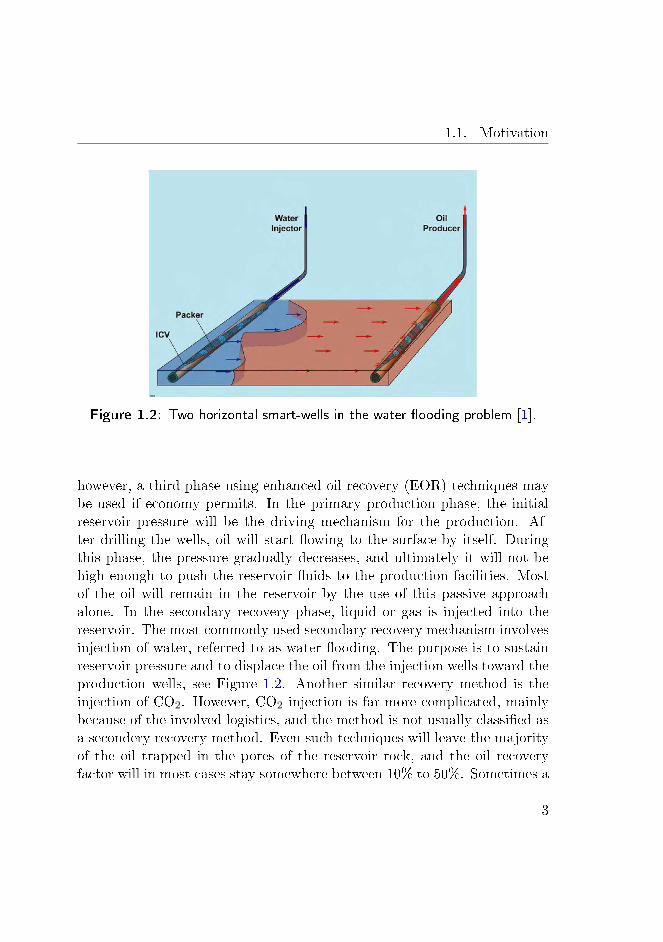
Figure 1.2: Two horizontal smart-wells in the water ooding problem [1].
however, a third phase using enhanced oil recovery (EOR) techniques maybe used if economy permits. In the primary production phase, the initialreservoir pressure will be the driving mechanism for the production. Af-ter drilling the wells, oil will start owing to the surface by itself. Duringthis phase, the pressure gradually decreases, and ultimately it will not behigh enough to push the reservoir uids to the production facilities. Mostof the oil will remain in the reservoir by the use of this passive approachalone. In the secondary recovery phase, liquid or gas is injected into thereservoir. The most commonly used secondary recovery mechanism involvesinjection of water, referred to as water ooding. The purpose is to sustainreservoir pressure and to displace the oil from the injection wells toward theproduction wells, see Figure 1.2. Another similar recovery method is theinjection of CO2. However, CO2 injection is far more complicated, mainlybecause of the involved logistics, and the method is not usually classied asa secondery recovery method. Even such techniques will leave the majorityof the oil trapped in the pores of the reservoir rock, and the oil recoveryfactor will in most cases stay somewhere between 10% to 50%. Sometimes a
3
1. Introduction
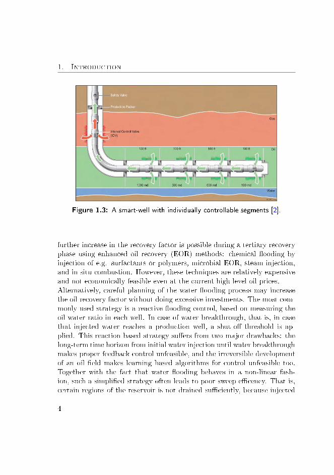
Figure 1.3: A smart-well with individually controllable segments [2].
further increase in the recovery factor is possible during a tertiary recoveryphase using enhanced oil recovery (EOR) methods: chemical ooding byinjection of e.g. surfactants or polymers, microbial EOR, steam injection,and in-situ combustion. However, these techniques are relatively expensiveand not economically feasible even at the current high level oil prices.Alternatively, careful planning of the water ooding process may increasethe oil recovery factor without doing excessive investments. The most com-monly used strategy is a reactive ooding control, based on measuring theoil-water ratio in each well. In case of water breakthrough, that is, in casethat injected water reaches a production well, a shut-o threshold is ap-plied. This reaction based strategy suers from two major drawbacks: thelong-term time horizon from initial water injection until water breakthroughmakes proper feedback control unfeasible, and the irreversible developmentof an oil eld makes learning based algorithms for control unfeasible too.Together with the fact that water ooding behaves in a non-linear fash-ion, such a simplied strategy often leads to poor sweep ecency. That is,certain regions of the reservoir is not drained suciently, because injected
4
1.1. Motivation
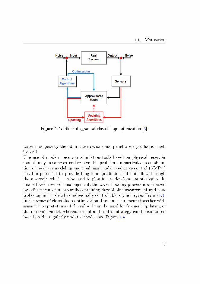
Figure 1.4: Block diagram af closed-loop optimization [3].
water may pass by the oil in those regions and penetrate a production wellinstead.The use of modern reservoir simulation tools based on physical reservoirmodels may to some extend resolve this problem. In particular, a combina-tion of reservoir modeling and nonlinear model predictive control (NMPC)has the potential to provide long-term predictions of uid ow throughthe reservoir, which can be used to plan future development strategies. Inmodel based reservoir management, the water ooding process is optimizedby adjustment of smart-wells containing down-hole measurement and con-trol equipment as well as individually controllable segments, see Figure 1.3.In the sense of closed-loop optimization, these measurements together withseismic interpretations of the subsoil may be used for frequent updating ofthe reservoir model, whereas an optimal control strategy can be computedbased on the regularly updated model, see Figure 1.4.
5
1. Introduction
1.2 Literature Review
Research on optimization of oil reservoirs using gradient based algorithmsand the adjoint approach for gradient computation has been conducted byother authors. There are three major topics when it comes to optimizationof oil reservoirs: optimal well placement, history matching and productionoptimization. Both optimal well placement and history matching are outsidethe scope of this work. We will therefore only briey comment on thesetwo subjects. Regarding production optimization, we will mainly focuson research that involves the adjoint method, when applied to the waterooding process.Drilling of wells is extremely expensive. Thus, determination of the number,type and location of wells are among the most important decision factors inthe early stages of reservoir development planning. Optimal well placementis therefore an issue of ongoing research [4, 5, 6]. Common for these groupsis the use of gradient based optimization algorithms and the adjoint modelfor gradient computation.The rst applications of gradient based optimization using the adjoint ap-proach in the oil production industry was for history matching. Historymatching used for reservoir optimization was pioonered by [7, 8].Within the research area of production optimization, [9] was among therst to formulate the problem of production optimization in the context ofan optimal control problem, using the adjoint method for gradient compu-tation of the objective function. His work was mainly focused on tertiaryrecovery techniques, such as chemical ooding. Later, [10, 1] optimized thewater ooding process, see Figure 1.2, and demonstrated that smart-welltechnology, see Figure 1.3, combined with optimal control has the potentialto increase net present value (NPV) of a reservoir. Through their work,gradient based optimization using the adjoint model has received signi-cant attention in the society of petroleum engineers. Smart-wells are eithercompleted with bang-bang type valves, i.e. on-o valves, or completed withvariable-setting valves. It has been shown that the shape of the optimal solu-tions will sometimes be of the bang-bang type [11, 12]. This type of solutionwas also to some extent demonstrated in [10, 1]. Solutions of the bang-bang
6
1.2. Literature Review
type may be implemented with simple on-o valves, which has the advan-tage of being less expensive than variable-setting valves. That is why theshape of optimal solutions is still an open issue in the reservoir commuity.Based on their work, several research groups have become interested in theuse of smart-well technology combined with optimal control. Common forall groups is the use of gradient based optimization methods that include theadjoint model for gradient computation [13, 14, 15, 16, 17]. Numerous otherissues related to production optimization of oil reservoirs are open to ongo-ing research. In particular, state constraint handling [18, 14, 15, 19, 20, 21],which is a very important topic in practical reservoir management, e.g.bounds on the reservoir pressure to avoid fracturing of the reservoir rock orlimits on the amount of produced water. Another topic of relevance, is thecalculation of the second derivative, the Hessian, of the objective function.The most common approach is to use BFGS approximations of the Hessian.However, to gain more accuracy and better convergence toward an optimalsolution, second order adjoints may be an alternative [22].Both history matching and production optimization are building blocks ina closed-loop optimizer, see Figure 1.4, in which the red loop represents thehistory matching, while the blue loop represents the production optimiza-tion. Production optimization is an open-loop optimizer, which is basedon response from the reservoir model, whereas history matching updatesthe model based on production data and seismic interpretations. Long-term reservoir management requires a closed loop approach, where prop-erties such as permeability and porosity of the reservoir rock are updatedfrequently and uncertainties on such properties are quantied. It is mostcommon to close the loop using the ensemble Kalman lter (EnKF) forhistory matching in conjunction with a gradient based algorithm for pro-duction optimization. The EnKF provides model updates and quantiesmodel uncertainties based on an ensemble of dierent reservoir properties,e.g. ensembles of permeability and porosity. Some of the earliest attemptsof linking the EnKF and gradient based optimization using the adjointmodel for gradient computation can be found in [23, 10, 24, 25, 26]. Therehas also been attempts on combining an estimator and an optimizer, whereboth production data mists and production optimization has been com-
7

1. Introduction
puted using the adjoint approach [27, 28]. However, the methods describedabove for history matching and production optimization all have the poten-tial to increase the economic value of an oil reservoir. This is demonstratedin a recent benchmark study of the water ooding process performed on asynthetic data set [29].
1.3 Objectives and Main Contributions
The primary objective of the work in this thesis is the implementation of aframework for oil production optimization by water ooding. We will usean explicit singly diagonally implicit Runge-Kutta (ESDIRK) method asa tool for ecient integration of the reservoir model. To achieve this wemust understand the underlying processes of both reservoir simulation andmethods for production optimization. Reservoir models may generate large-scale optimization problems. That is why single-shooting using adjoints forgradient computation is the most widely used method for production opti-mization of oil reservoirs, and it is also the reason why we have chosen thismethod. Good convergence in the single-shooting method requires an e-cient and accurate numerical integration. ESDIRK methods with adaptivestep size control has such properties.Computation of adjoints involves the gradients of the model. These arecomputed by ESDIRK integration during simulations. Thus, to ecientlycompute the adjoints, we need an implementation of both model and inte-grator that facilitates the reuse of gradient information. This suggests thatwe need a reservoir simulator, a method for numerical integration and anadjoint model, where we have full access to the source code.For the simulation we implement a two-phase ow simulator. We spatiallydiscretize the ow equations by the nite volume method (FVM), in whichwe use the two-point ux approximation (TPFA) and single-point upstream(SPU) weighting of the uid terms. We use vertical injection and productionwells of the Peaceman type.For the numerical integration we develop and implement mass conservingESDIRK methods with embedded error estimators for adaptive step size
8

1.4. Outline
control. The two-phase ow problem is based on conservation of mass. Wepropose a new dierential equation model that upon temporal discretizationmaintains such a property. The spatially discretized two-phase ow problemcan be directly formulated using this model.For the optimization we use a gradient based algorithm, in which we includethe adjoint model for computing the gradient of the objective function. Weuse BFGS updates for computing the Hessian of the objective function. Wedo not have access to any real production data, thus, we perform open-loopoptimization (the blue loop in Figure 1.4). We focus on optimal controlof injection rates and bottom hole pressures (BHPs) of injection wells andproduction wells, respectively. The objective is to increase oil productionusing water ooding and thereby maximize net present value (NPV) of thereservoir.The main contributions of this work are:
• The formulation of a new dierential equation model that upon tem-poral discretization maintains the mass conserving property of thespatially discretized two-phase ow problem.
• The development of mass conserving ESDIRK methods with embed-ded error estimators for adaptive step size control.
• The application of ESDIRK integration and error based step size con-trol for computation of the water ooding process.
To our knowledge, there have been no previous attempts on applying ES-DIRK methods and error based step size control for computation of thewater ooding process. Neither for commercial purposes nor in simulatorsdeveloped for research purposes, with exception of the work that we presentin this thesis and in the papers A - E, included in this thesis.
1.4 Outline
This thesis is divided into 5 chapters and 8 appendices. The backgroundand motivation behind the project is given in Chapter 1. The model of
9

1. Introduction
the combined ow of water and oil in a reservoir is decribed in Chapter2, together with a description of the well models. The reservoir model isessentially a system of partial dierential equations. The methods for spatialand temporal discretization that we use to extract the solution from thissystem is given in Chapter 3 and 4, respectively. In Chapter 5 we presentthe water ooding process and the problem of maximizing net present valueof a reservoir. Chapter 6 concludes the study.In Appendix A we describe the derivation of selected Jacobian elementsin details. Appendix B includes the coecients for the numerical integra-tion methods. Appendix C contains a list of the physical quantities thatdescribes the reservoir model and the well models along with a list of com-monly used abbreviations. In appendix D - H we include ve conferencepapers A - E that have been reviewed, presented and published in proceed-ings. The material presented in the papers and in the thesis overlap to someextend. However, they are complementary, since both contain details thatare not presented elsewhere.
10
CHAPTER 2Reservoir Model
Oil reservoirs are characterized by complex geometry, spatially variable ge-ological properties, e.g. porosity and permeability of a porous medium, andcomplex uid mixtures of water and multiple oil and gas components. Inreservoir simulation, we are interested in describing the transport of thesedierent components through the porous medium. In general, a componentcan exist in any uid phase, and as a result we must solve one equationper component times a set of phase equilibrium relations. Compositionalreservoir models, which treats every component in every uid phase individ-ually, are computationally expensive to simulate, even with today's modernsupercomputers. The complexity of the model can be reduced by lump-ing the hydrocarbon components into pseudo components. The black oilmodel, which is common in the petroleum industry, is a simplied isother-mal compositional reservoir model. Besides water, it contains only twopseudo hydrocarbon components: oil and gas. In the black oil model it isassumed that water and oil are immiscible, and that water does not vaporizeinto the gas phase. Thus, the water phase consists of the water componentalone. The gas can dissolve in both the water phase and the oil phase, andit is not uncommon that black oil models allow oil to vaporize into the gas
11

2. Reservoir Model
phase.With respect to computation time it is less demanding to simulate the blackoil model compared to compositional simulation. However, the physics aretreated less realistically in the black oil formulation. Because of the reducedcomputational cost of the black oil model, this formulation is relevant inproduction optimization, which requires frequent updating/simulation ofthe reservoir model. In the present work we use a simplied version of theblack oil formulation: a two-phase system containing only water and oilwith complete immiscibility [30, 31, 32, 33, 34]. The simplication elimi-nates the phase equilibrium relation due to the solubility of gas in the oilphase. In this way we reduce the computational cost per simulation. Thesimplied description of the reservoir uids is sucient for demonstratingthe production optimization technique utilized in Chapter 5.This chapter is organized as follows. In the rst two sections we presentthe equations that govern the two-phase ow problem together with theinitial and boundary conditions. In Section 2.3 we describe the constutivemodels, divided into properties concerning the reservoir rock and propertiesconcerning the reservoir uids. Section 2.4 describes the transport modelgoverned by Darcy's law. The well models [35] that we use are presentedin Section 2.5. Finally, in Section 2.6 we discuss how to derive the primaryvariables of the system.
2.1 Governing Equations
Consider the spatial domain Ω ⊂ R3 and the time domain T = t ∈ R : t ≥0. The boundary of the spatial domian is ∂Ω ⊂ R3 and the boundary of thetime domain is ∂T = t ∈ R : t = 0. The water and oil phases are indexedas α ∈ w, o. Let Cα = Cα(t, s), be the mass concentrations of water andoil in the reservoir (mass per unit volume of reservoir) as functions of timet ∈ T and position s ∈ Ω. The mass balances of the reservoir uids areexpressed by the following system of partial dierential equations
∂Cα∂t
= −∇ · Fα +Qα t ∈ T \ ∂T s ∈ Ω \ ∂Ω (2.1)
12
2.2. Initial and Boundary Conditions
Qinjα Qproα
Ω ∂Ω
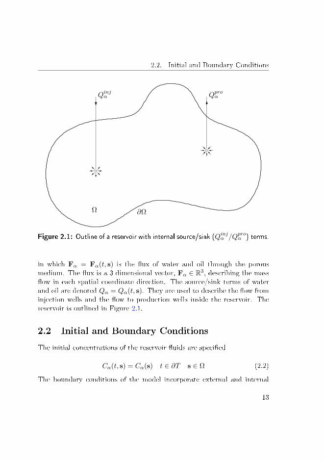
Figure 2.1: Outline of a reservoir with internal source/sink (Qinjα /Qproα ) terms.
in which Fα = Fα(t, s) is the ux of water and oil through the porousmedium. The ux is a 3-dimensional vector, Fα ∈ R3, describing the massow in each spatial coordinate direction. The source/sink terms of waterand oil are denoted Qα = Qα(t, s). They are used to describe the ow frominjection wells and the ow to production wells inside the reservoir. Thereservoir is outlined in Figure 2.1.
2.2 Initial and Boundary Conditions
The initial concentrations of the reservoir uids are specied
Cα(t, s) = Cα(s) t ∈ ∂T s ∈ Ω (2.2)
The boundary conditions of the model incorporate external and internal
13

2. Reservoir Model
conditions. External boundary conditions dene spatial limits of the reser-voir. Internal boundary conditions dene well placements. Both externaland internal conditions are specied by dening ow rates across a boundaryor pressure at a boundary, which corresponds to Neumann or Dirichlet typeconditions. For external boundaries we will assume a Neumann conditioncorresponding to no ow across the reservoir boundaries
Fα(t, s) = 0 t ∈ T s ∈ ∂Ω (2.3)
Internal boundaries due to injection and production wells are treated seper-ately in Section 2.5.
2.3 Constitutive Models
The concentrations of water and oil in the reservoir may be expressed as
Cα = φραSα (2.4)
φ is the porosity of the reservoir rock. ρα = ρα(Pα) is the density ofeach reservoir uid in particular. The density depends on the pressurePα = Pα(t, s) in the uid. Sα = Sα(t, s) is the saturation of the uid. Thesaturation represents the volumetric fraction of the uid occupying the voidspace (pore space volume). As water and oil jointly ll the entire void spaceof the reservoir, the following saturation constraint holds
Sw + So = 1 (2.5)
Water and oil are transported by convection through the porous medium.Therefore, the uxes can be expressed as
Fα = ραuα (2.6)
uα = uα(Pw, Sw) are the velocities at which the uid phases individuallyow through the porous medium. They are modelled in terms of Darcy owin Section 2.4.
14
2.3. Constitutive Models
To complete the two-phase ow model we must introduce several otherquantities, namely permeability, relative permeability, capillary pressureand viscosity. Porosity and permeability are quantities that characterizethe porous medium in which the reservoir uids reside. Density, relativepermeability, capillary pressure and viscosity are all properties of the reser-voir uids. In the following we will describe these quantities and providethe models needed for completing the two-phase ow model.
2.3.1 Porosity
The reservoir uids are trapped inside the pores of a porous medium, e.g.chalk or sandstone formations. The porosity is the volumetric fraction ofthe total bulk volume that is not occupied by solid matter (reservoir rock),ie. it is the fraction of the total bulk volume that may contain the reservoiruids (water, oil). Let V be the total bulk volume of the reservoir and letVp be the pore volume (PV), i.e. void space of the reservoir rock, then theporosity is dened as φ = Vp/V . Since changes in rock characteristica arenot included in our model, the porosity is constant over time but may varyat dierent locations in the reservoir, such that φ = φ(s).
2.3.2 Permeability
The permeability is a measure of the capacity of a porous medium to conductuids through its interconnected pores. It is dened for single-phase owand often referred to as absolute permeability. The concept of permeabilityis of importance in determining the connectivity and preferred ow directionin the reservoir. The permeability is dened as a tensor k of size 3× 3. Intheory k is a full tensor, however, in many practical situations it is possibleto assume that k is a diagonal tensor given by
k =
kxx 0 00 kyy 00 0 kzz
(2.7)
15
2. Reservoir Model
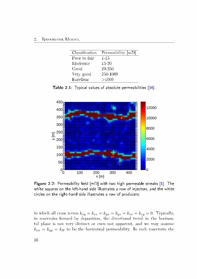
Classication Permeability [mD]
Poor to fair 1-15Moderate 15-20Good 20-250Very good 250-1000Excellent >1000
Table 2.1: Typical values of absolute permeabilities [34].
x [m]
y [m
]
0 100 200 300 4000
50
100
150
200
250
300
350
400
450
0
2000
4000
6000
8000
10000
12000
Figure 2.2: Permeability eld [mD] with two high permeable streaks [1]. Thewhite squares on the left-hand side illustrates a row of injectors, and the whitecircles on the right-hand side illustrates a row of producers.
in which all cross terms kxy = kxz = kyx = kyz = kzx = kzy = 0. Typically,in reservoirs formed by deposition, the directional trend in the horizon-tal plane is not very distinct or even not apparent, and we may assumekxx = kyy = kH to be the horizontal permeability. In such reservoirs the
16
2.3. Constitutive Models
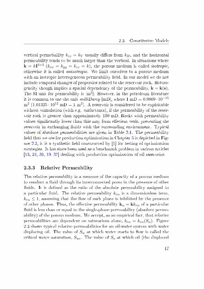
vertical permebaility kzz = kV usually diers from kH , and the horizontalpermeability tends to be much larger than the vertical. In situations wherek = kI3×3 (kxx = kyy = kzz = k), the porous medium is called isotropic,otherwise it is called anisotropic. We limit ourselves to a porous mediumwith an isotropic heterogeneous permeability eld. In our model we do notinclude temporal changes of properties related to the reservoir rock. Hetero-geneity though implies a spatial dependency of the permeability, k = k(s).The SI unit for permeability is [m2]. However, in the petroleum literatureit is common to use the unit milliDarcy [mD], where 1 mD = 0.9869 · 10−15
m2 (1.01325 · 1012 mD = 1 m2). A reservoir is considered to be exploitablewithout stimulation (with e.g. surfactants), if the permeability of the reser-voir rock is greater than approximately 100 mD. Rocks with permeabilityvalues signicantly lower than this may form eecient seals, preventing thereservoir in exchanging uids with the surrounding environment. Typicalvalues of absolute permeabilities are given in Table 2.1. The permeabilityeld that we use for production optimization in Chapter 5 is depicted in Fig-ure 2.2, it is a synthetic eld constructed by [1] for testing of optimizationstrategies. It has since been used as a benchmark problem in various articles[13, 24, 36, 19, 37] dealing with production optimization of oil reservoirs.
2.3.3 Relative Permeability
The relative permeability is a measure of the capacity of a porous mediumto conduct a uid through its interconnected pores in the presence of otheruids. It is dened as the ratio of the absolute permeability assigned toa particular uid. The relative permeability krα is a dimensionless term.krα ≤ 1, assuming that the ow of each phase is inhibited by the presenceof other phases. Thus, the eective permeability kα = kkrα of a particularuid is less than or equal to the single-phase permeability (absolute perme-ability) of the porous medium. We accept, as an empirical fact, that relativepermeabilities are dependent on saturations alone, krα = krα(Sα). Figure2.3 shows typical relative permeabilities for an oil-water system with waterdisplacing oil. The value of Sw at which water starts to ow is called thecritical water saturation, Swc. The value of So at which oil (the displaced
17
2. Reservoir Model
0 0.1 0.2 0.3 0.4 0.5 0.6 0.7 0.8 0.9 10
0.1
0.2
0.3
0.4
0.5
0.6
0.7
0.8
0.9
1
← Swc
1−Sor
→
Sw
k rα
k
rw
kro
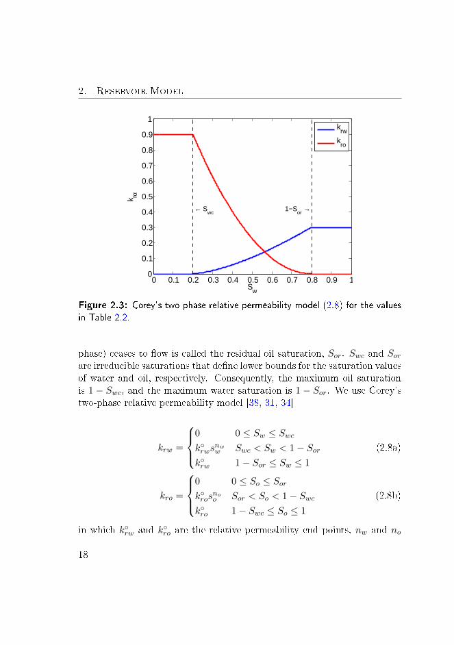
Figure 2.3: Corey's two-phase relative permeability model (2.8) for the valuesin Table 2.2.
phase) ceases to ow is called the residual oil saturation, Sor. Swc and Sorare irreducible saturations that dene lower bounds for the saturation valuesof water and oil, respectively. Consequently, the maximum oil saturationis 1 − Swc, and the maximum water saturation is 1 − Sor. We use Corey'stwo-phase relative permeability model [38, 31, 34]
krw =
0 0 ≤ Sw ≤ Swckrws
nww Swc < Sw < 1− Sor
krw 1− Sor ≤ Sw ≤ 1
(2.8a)
kro =
0 0 ≤ So ≤ Sorkros
noo Sor < So < 1− Swc
kro 1− Swc ≤ So ≤ 1
(2.8b)
in which krw and kro are the relative permeability end points, nw and no
18

2.3. Constitutive Models
Symbol Description Value Unit
Swc Critical water saturation 0.2 -Sor Residual oil saturation 0.2 -krw Water end point relative permeability 0.3 -kro Oil end point relative permeability 0.9 -nw Water Corey exponent 1.5 -no Oil Corey exponent 2.0 -
Table 2.2: The values used for illustration of the Corey's two-phase relativepermeability model (2.8) in Figure 2.3.
are the Corey exponents and sw and so are the normalized saturations
sw =Sw − Swc
1− Swc − Sor(2.9a)
so =So − Sor
1− Swc − Sor(2.9b)
of the water phase and the oil phase. Figure 2.3 is constructed using theparameters in Table 2.2.
2.3.4 Capillary Pressure
In immiscible oil-water systems, water is most often wetting the surface ofthe reservoir rock, meaning that water tends to maintain contact with therock, thus displacing the oil. Due to interfacial tension between the non-wetting and the wetting phase uids, the pressure in the non-wetting uid ishigher than the pressure in the wetting uid. The dierence between thesetwo pessures is the capillary pressure
Pcow = Po − Pw (2.10)
Empirically, it is accepted, that the capillary pressure depends on the sat-uration of the wetting uid, such that Pcow = Pcow(Sw). Eects due to
19

2. Reservoir Model
capillarity becomes less signicant in highly permeable and highly porousmedia. In dense formations with very small pores, capillarity introduces adiusive term into (2.1) [39]. However, we assume zero capillary pressure
Pcow = 0 (2.11)
since no additional insight for the optimization problem is gained by includ-ing capillarity.
2.3.5 Density
Depending upon how uids respond to pressure, they can be classied ascompressible, slightly compressible or incompressible. Constant water den-sity is normally a valid assumption. Some oil components may exhibit sig-nicant density changes with pressure, especially if the oil phase containslarge quantities of dissolved gas. For a gas phase compressibility is veryimportant. However, we consider a water/oil system, in which we assumeboth the water phase and the oil phase to behave like slightly compressibleuids at reservoir conditions. For isothermal conditions the compressibilityof a uid is dened by
cα =1
ρα
∂ρα∂Pα
∣∣∣∣T
(2.12)
where ρα = ρα(Pα) is the uid density (at constant temperature T ). As-suming the uid compressibility to be constant over the pressure range ofinterest, integration of (2.12) yields the following equation of state
ρα = ραecα(Pα−P
α) (2.13)
where ρα is the density at reference pressure Pα. The relation (2.13) between
density and pressure is depicted in Figure 2.4 using the reference values inTable 2.3. Using a Taylor series expansion, we see that
ρα = ρα
[1 + cα(Pα − P α) +
1
2!c2α(Pα − P α)2 + · · ·
](2.14)
20

2.3. Constitutive Models
150 160 170 180 190 200 210 220 230 240 2501001
1002
1003
Pw [atm]
ρ w [k
g/m
3 ]
150 160 170 180 190 200 210 220 230 240 250801
802
803
Po [atm]
ρ o [kg/
m3 ]
Figure 2.4: The uid density (2.13) for the values in Table 2.3.
Symbol Description Value Unit
ρw Water density (at 1 atm) 1000 kg·m−3
ρo Oil density (at 1 atm) 800 kg·m−3
cw Water compressibility 10−5 atm−1
co Oil compressibility 10−5 atm−1
Table 2.3: The values used for illustration of the uid density (2.13) in Figure2.4.
and since we assume the uids to be only slightly compressible, i.e. thecompressibility cα is small (typically in the range from 10−10 to 10−9 Pa−1
[34]), we can neglect all high order terms and approximate (2.13) with thelinear relationship
ρα ≈ ρα[1 + cα(Pα − P α)] (2.15)
using a reference density and pressure at reservoir conditions.
21
2. Reservoir Model
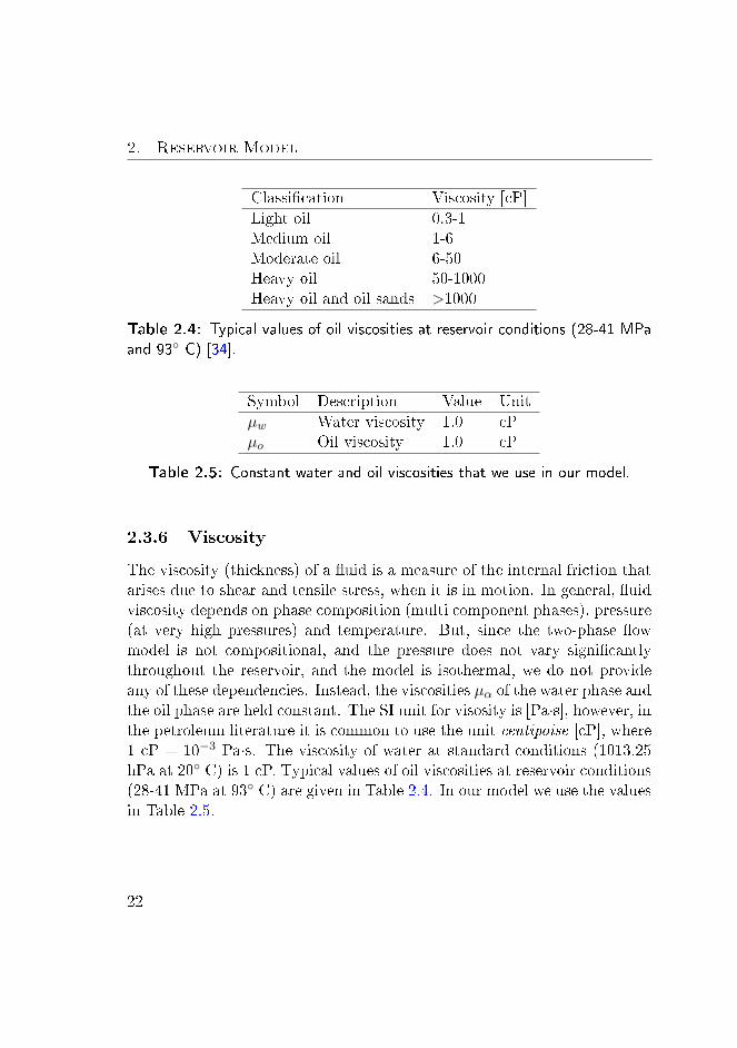
Classication Viscosity [cP]
Light oil 0.3-1Medium oil 1-6Moderate oil 6-50Heavy oil 50-1000Heavy oil and oil sands >1000
Table 2.4: Typical values of oil viscosities at reservoir conditions (28-41 MPaand 93 C) [34].
Symbol Description Value Unit
µw Water viscosity 1.0 cPµo Oil viscosity 1.0 cP
Table 2.5: Constant water and oil viscosities that we use in our model.
2.3.6 Viscosity
The viscosity (thickness) of a uid is a measure of the internal friction thatarises due to shear and tensile stress, when it is in motion. In general, uidviscosity depends on phase composition (multi component phases), pressure(at very high pressures) and temperature. But, since the two-phase owmodel is not compositional, and the pressure does not vary signicantlythroughout the reservoir, and the model is isothermal, we do not provideany of these dependencies. Instead, the viscosities µα of the water phase andthe oil phase are held constant. The SI unit for visosity is [Pa·s], however, inthe petroleum literature it is common to use the unit centipoise [cP], where1 cP = 10−3 Pa·s. The viscosity of water at standard conditions (1013.25hPa at 20 C) is 1 cP. Typical values of oil viscosities at reservoir conditions(28-41 MPa at 93 C) are given in Table 2.4. In our model we use the valuesin Table 2.5.
22

2.4. Transport Model
2.4 Transport Model
The ow of the reservoir uids is driven by spatial dierences in pressure(pressure gradient) and gravity. Fluid ow in a porous medium at low tomoderate velocities is governed by Darcy's law [40, 31]
uα = −λαk∇Φα (2.16)
in which λα = krαµα
is the phase mobility. Darcy's law is a linear relationshipbetween the phase velocity uα = uα(Pα, Sα) and the ow potential eld
∇Φα = ∇Pα − ραg∇z (2.17)
where ∇Pα is the pressure gradient, g is the gravitational acceleration andz is the depth (downward positive). We do not include gravitational eectsin the model, that is g = 0 in (2.17).
2.5 Well Models
Although we have not presented any method for spatial discretization yet,we will use the concept of grid blocks in this section. A grid block is anite control volume of the total bulk volume of the reservoir. We willprovide a detailed description of the nite volume approach in Chapter 3.Injection wells and production wells (injectors and producers) are locatedand perforated in a single grid block, e.g. as illustrated in Figure 2.5.Injectors are used for injection of the phase, which in our case is water,displacing the reservoir uids. Producers are used for prodution of thedisplaced reservoir uids. Let N be the set of grid blocks, I ⊂ N be theset of grid blocks containing an injector, and P ⊂ N be the set of gridblocks containing a producer. Thus, if i ∈ I then the ith grid block ispenetrated by an injection well, and if i ∈ P then it is penetrated by aproduction well. Injectors are operated at variable (volumetric) injectionrates, whereas producers are operated at variable bottom hole pressures(BHPs). The BHP is the pressure inside the well at reservoir depth.
23
2. Reservoir Model
Qinjα Qproα
Ω ∂Ω
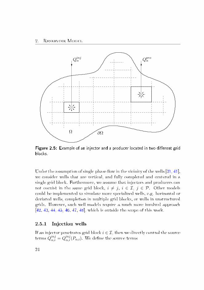
Figure 2.5: Example of an injector and a producer located in two dierent gridblocks.
Under the assumption of single-phase ow in the vicinity of the wells [31, 41],we consider wells that are vertical, and fully completed and centered in asingle grid block. Furthermore, we assume that injectors and producers cannot coexist in the same grid block, i 6= j, i ∈ I, j ∈ P. Other modelscould be implemented to simulate more specialized wells, e.g. horizontal ordeviated wells, completion in multiple grid blocks, or wells in unstructuredgrids. However, such well models require a much more involved approach[42, 43, 44, 45, 46, 47, 48], which is outside the scope of this work.
2.5.1 Injection wells
If an injector penetrates grid block i ∈ I, then we directly control the sourceterms Qinjα,i = Qinjα,i (Pα,i). We dene the source terms
24

2.5. Well Models
Qinjα,i =
(qinjα
V
)
i
i ∈ I (2.18a)
as the rate of injected mass qinjα,i of each phase averaged over the grid blockvolume Vi (the rate of injected mass per unit volume of reservoir). Usually,only water is injected to keep the pressure in the reservoir above a certainlevel, implying that
qinjw,i = (ρwqinj)i i ∈ I (2.19a)
qinjo,i = 0 i ∈ I (2.19b)
in which qinji is the volumetric injection rate of water into grid block i ∈ I.
2.5.2 Production wells
If a producer penetrates grid block i ∈ P, then we can only indirectlycontrol the sink terms Qproα,i = Qproα,i (Pα, Sα)i, since the produced liquid is acomposition of oil and water. We dene the sink terms
Qproα,i =
(qproα
V
)
i
i ∈ P (2.20a)
as the rate of produced mass qproα,i of each phase averaged over the grid blockvolume Vi (the rate of produced mass per unit volume of reservoir). Theset of producers are modelled as
qproα,i = −(WIραλα)i(Pα − P bh)i i ∈ P (2.21)
where WIi denotes the well index, and P bhi denotes the BHP of the pro-duction well in grid block i ∈ P. Each producer enters the reservoir modelthrough a well index. The well index captures the interaction between the
25

2. Reservoir Model
well and the reservoir, i.e. making the well model account for both geomet-ric characteristics of the well and properties of the surrounding reservoirrock. Specically, for each grid block i ∈ P containing a well, the quantityWIi relates the ow rate of the well to the local BHP and the pressure in thegrid block. For vertical wells in non-square Cartesian grids (cuboid grids)with anisotropic permeability elds (assuming diagonal tensors), Peaceman[35] derived an analytical expression for WIi. The Peaceman well index isgiven as
WIi =
(θ√kxxkyyh
ln(re/rw) + s
)
i
i ∈ P (2.22)
θ is the angle open to ow (e.g. 2π for a well in the interior and π2 for
a corner well), kxx and kyy are permeability components in the x- and y-directions as dened in (2.7), ∆x and ∆y are the grid block sizes, h is theheight of the well (grid block height in the z-direction), rw is the wellboreradius, and
re,i = 0.28
√√kyy/kxx∆x2 +
√kxx/kyy∆y2
4√kyy/kxx + 4
√kxx/kyy
i
i ∈ P (2.23)
is the equivalent radius. re is the radial position (centered around the well)at which the pressure in the well block, computed by the simulator, is equalto the pressure obtained by the analytical model. The skin s in (2.22) is adimensionless factor included to match the theoretical productivity of thewell with actual conditions. Thus, the skin factor accounts for damage or in-uences that are impairing the well productivity, or stimulation (fracturing,acidization, etc.) that enhances productivity. We assume ideal conditions,that is s = 0.
26
2.6. State Transformation
2.6 State Transformation
Considering the algebraic constraints (2.5) and (2.11), we dene
S = Sw = 1− So (2.24a)
P = Po = Pw (2.24b)
where S = S(t, s) is the saturation of water, and P = P (t, s) is the phasepressure (reservoir pressure, since Po = Pw). Throughout the rest of thisthesis we will refer to S and P as saturation and pressure respectively. Inthe two-phase ow model (2.1) - (2.17), we may use (S, P ) as state variablesinstead of (Cw, Co). (2.4), (2.5), (2.10) and (2.11) may be used to computeS and P given Cw and Co. Implying that we may state the initial conditions(2.2) as initial saturation and pressure
S(t, s) = S(s) t ∈ δT s ∈ Ω (2.25a)
P (t, s) = P (s) t ∈ δT s ∈ Ω (2.25b)
2.7 Summary
We have described the two-phase ow problem, the well models, and theprimary variables of the model. The two phases are oil and water. Themodel consists of two partial dierential equations representing conservationof mass. Mass is transported by convection at a velocity determined byDarcy's law. Relative permeabilites are determined by a Corey expressionand we assume zero capillary pressure. The uid densities are describedby an equation of state relating the densities to pressure. The porosity ishomogeneous and we assume a heterogenous isotropic permeability eld.We use vertical injection and production wells of the Peaceman type. Theprimary variables of the model are reservoir pressure and water saturation.
27

CHAPTER 3Spatial Discretization
In this chapter, we describe how we obtain the discrete representations forthe spatial derivative operators in the two-phase ow equations (2.1). Forthe purpose of spatial discretization we have a variety of methods to choosefrom. Most of the methods are variations and combinations of three wellknown methods: the nite dierence method (FDM), the nite volumemethod (FVM), and the nite element method (FEM).The FDM is considered the oldest of the three methods, and because of itssimplicity and intuitive approach it is still widely used [49, 34]. The methodrepresents the spatial derivatives in discrete grid points. FD schemes aresuciently robust and ecient for a large number of problems, and exten-sions to higher order approximations of the solution is relatively straight-forward to obtain. However, higher order nite dierence stencils are oftenconstructed locally for each spatial dimension. This limits the geometricexibility of the method, making it less suitable for handling domains withcomplex geometry, e.g. in terms of local grid renements for dealing withabrupt changes in absolute permeability.The FVM is a control volume formulation that uses an element based dis-cretization. Due to the control volume formulation, FVMs maintain local
29
3. Spatial Discretization
conservation of mass, energy and momentum, which cannot in general beguaranteed for FDMs. The FVM represents the physical domain by a col-lection of small control volumes that jointly ll the entire domain. Theelements may have dierent sizes and may be organized in an unstruc-tured manner. The solution is approximated on the element by the cellaverage at the center of the element. The classic nite volume scheme ispurely local, thus, no limitations are imposed on the grid structure, andthe method generalizes easily to unstructured grids in higher dimensions.This ensures geometric exibility of the method. The FVM reduces theux term to a surface integral by the use of Gauss' divergence theorem, andtherefore we must evaluate the uxes at the boundaries. The interface uxbetween neighbouring elements is most often computed by the two pointux approximation (TPFA) [32, 65, 50]. The TPFA is a low order approx-imation. High order approximations are not straightforward to obtain inunstructured grids, which is one of the major drawbacks of the FVM. Highorder reconstructions of interface values by the use of multi point ux ap-proximations (MPFA) involve information from more than two cells. Thisintroduces the need for particular grid structures, which jeopardizes thegeometric exibility of the FVM in higher dimensions. In particular, forporous media ow in an anisotropic permebaility eld on non-k-orthogonalgrids, TPFA gives an error in the solution [51, 52]. However, to be able tosolve the ow equations on general grids, variations of both TPFA [53] andMPFA [54, 55, 56, 57, 58] methods have been suggested.The FEM has initially been developed for structural stress analysis. As thename of the method suggests, it is element based. It ensures geometric ex-ibility and allow dierent element sizes. A recent employment of the FEMin reservoir simulation can be found in [59]. High order discrete approxi-mations of the solution are relatively simple to obtain in the nite elementsetting. In particular, local basis functions allows for dierent orders of ap-proximation in each element. However, the basis functions are symmetricin space, and this may cause stability issues for problems based on conser-vation laws, in which information ows in specic directions. These issuesmay be solved by the discontinuous Galerkin nite element method (DG-FEM). The DG-FEM is basically a hybrid between the FEM and FVM.
30

3.1. Nomenclature
The method ensures exibility both in terms geometry and in the choiceof the numerical ux, high order approximations are relatively simple toobtain on general grids, and it maintains local conservation. On the nega-tive side, the number of unknowns increases and DG-FEM solvers can becomputationally expensive in comparison to FVM and FEM solvers. How-ever, because of the appealing properties, the method is gaining interest inreservoir simulation [60, 61, 62] and a general description of the DG-FEMis found in [63].Because of the close relation to the conservation laws, we have chosen theFVM for spatial discretization. We assume an isotropic permeability eld,thus, we use the TPFA to reconstruct the discrete ux terms. In Section 3.1and 3.2 we describe how we derive the spatially dicretized ow equations.Section 3.3 discusses how to evaluate the transmissibilities. In Section 3.4we present a new dierential equation model for the spatially dicretized owequations, as proposed in Paper A. Finally, in the last section we illustratethe Jacobian structure of the spatially discretized model.
3.1 Nomenclature
For the nite volume approach, we divide the spatial domain Ω into Nsubregions Ωi with boundaries ∂Ωi, i ∈ N = 1, 2, . . . , N, such that
⋃
i∈NΩi = Ω (3.1a)
(Ωi\∂Ωi) ∩ (Ωj\∂Ωj) = ∅ i, j ∈ N i 6= j (3.1b)
where N is the set of indices of non-overlapping control volumes that coverthe whole domain Ω. This is illustrated in Figure 3.1. In the followingwe will use Figure 3.1 to explain the problem setup and the symbols used.Dene
γij = Ωi ∩ Ωj i, j ∈ N i 6= j (3.2)
and for the ith control volume Ωi, let N (i) ⊂ N denote the set of indices ofneighbouring subregions. Then
31
3. Spatial Discretization
γij = Ωi ∩ Ωj i ∈ N j ∈ N (i) (3.3)
denotes the interface between two adjacent control volumes. In particular
γij 6= ∅ i ∈ N j ∈ N (i) (3.4a)
γij = ∅ i ∈ N j /∈ N (i) (3.4b)
Each control volume contains a nodal point. Properties of the model arerepresented at the nodal points as the average over the control volumessurrounding them. The nodal point of the ith control volume is locatedsuch that
si ∈ Ωi i ∈ N (3.5)
and we dene
sij = sj − si i ∈ N j ∈ N (i) (3.6)
as the internode connection between the grid node locations of two neigh-bouring grid blocks i and j. For the discrete spatial domain we assumethat
sij ⊥ γij i ∈ N j ∈ N (i) (3.7)
by construction. Figure 3.1 illustrates a 2-D grid maintaining the propertyin (3.7). Because the location of the grid nodes si and sj are taken asthe circumcenters of each block, we see that sij (perpendicular) bisects theinterface γij , in this particular example.For the spatial discretization below we use the following notation: ψij meansthat we evaluate the property ψ at the interface γij , and ψi means that weevaluate the property ψ at the nodal point si. In particular, for propertiesdepending on both time and space we have ψi = ψ(t, si), and for timeinvariant properties that only depend on space we have ψi = ψ(si).
32

3.2. Finite Volume Approach
Qinjα Qproα
Ω
Ωj
sjsi
sij γij
nij
∂Ω
Ωi
∂Ωj
∂Ωi
Figure 3.1: A reservoir spatially discretized by the FVM.
3.2 Finite Volume Approach
By integration of (2.1) over the control volume Ωi we obtain the integralform of the governing equations
∂
∂t
∫
Ωi
CαdV = −∫
Ωi
∇ · FαdV +
∫
Ωi
QαdV i ∈ N (3.8)
The volume integral on the left-hand side in (3.8), the accumulation term,is discretized using the average value of the accumulated mass Cα over thecontrol volume
∫
Ωi
CαdV ≈ (CαV )i i ∈ N (3.9)
33

3. Spatial Discretization
The volume integral in the second term on the right-hand side in (3.8), thesource term, is discretized using the average value of the source Qα over thecontrol volume
∫
Ωi
QαdV ≈ (QαV )i i ∈ N (3.10)
In particular, Qα,i = 0, i /∈ I∪P. Remember that I is dened in Section 2.5as the set of indices of grid blocks containing an injector, and P is denedas the set of indices of grid blocks containing a producer.The volume integral in the rst term on the right-hand side in (3.8), theconvective (ux) term, is rewritten as an integral over the entire boundingsurface of the control volume by application of Gauss' divergence theorem
∫
Ωi
∇ · FαdV =
∫
∂Ωi
n · FαdA i ∈ N (3.11)
where n is a unit vector normal to the surface elements dA of control volumeΩi. Using (3.4), we may rewrite (3.11) as follows
∫
Ωi
∇ · FαdV =∑
j∈N (i)
∫
γij
n · FαdA i ∈ N (3.12)
in which we sum over interfaces between the ith control volume and itsneighbouring subregions Ωj , j ∈ N (i). We approximate the surface integralsin (3.12) using the midpoint rule
∫
Ωi
∇ · FαdV ≈∑
j∈N (i)
(n · FαA)ij i ∈ N (3.13)
where nij is the normal vector of interface γij (pointing outwards in relationto Ωi), Fα,ij is the ux across interface γij , and Aij is the area of interfaceγij . We now evaluate the uxes across the interfaces using the TPFA.Remembering (2.6), (2.16), (2.17), and neglecting gravity, the ux acrossinterface γij becomes
Fα,ij = −(ραλαk∇P )ij i ∈ N j ∈ N (i) (3.14)
34

3.2. Finite Volume Approach
where the properties ρα,ij , λα,ij , kij , and the pressure gradient ∇Pij areevaluated at interface γij . Substituting the ux in (3.13) with (3.14) yields
∫
Ωi
∇ · FαdV ≈ −∑
j∈N (i)
nij · (ραλαk∇P )ijAij
= −∑
j∈N (i)
Aij(ραλα)ijnij · (k∇P )ij
i ∈ N (3.15)
We only consider isotropic permeability elds, kij = kijI. Consequently
∫
Ωi
∇ · FαdV ≈ −∑
j∈N (i)
(Ak)ij(ραλα)ijnij · ∇Pij i ∈ N (3.16)
The ux over interface γij is driven by the pressure gradient ∇Pij . For theTPFA we use a rst order approximation of the pressure gradient
∇Pij ≈(
∆P
∆s
s
∆s
)
ij
i ∈ N j ∈ N (i) (3.17)
where ∆Pij = Pj − Pi is the pressure dierence between the nodal pointssi and sj of two adjacent control volumes Ωi and Ωj . We dene sij =sj − si, such that ∆sij = |sij | is the internode distance between si and sj .Substitution of ∇Pij in (3.16) with (3.17) yields
∫
Ωi
∇ · FαdV ≈ −∑
j∈N (i)
(Ak)ij(ραλα)ijnij ·(
∆P
∆s
s
∆s
)
ij
i ∈ N (3.18)
which we rearrange
∫
Ωi
∇·FαdV ≈ −∑
j∈N (i)
(Ak
∆s
)
ij
(ραλα)ij∆Pijnij ·( s
∆s
)ij
i ∈ N (3.19)
Because of the relation in (3.7), the grid is constructed such that
35
3. Spatial Discretization
nij =( s
∆s
)ij
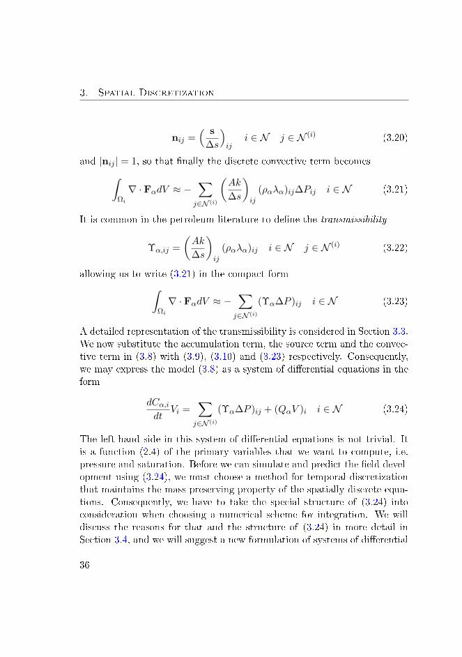
i ∈ N j ∈ N (i) (3.20)
and |nij | = 1, so that nally the discrete convective term becomes
∫
Ωi
∇ · FαdV ≈ −∑
j∈N (i)
(Ak
∆s
)
ij
(ραλα)ij∆Pij i ∈ N (3.21)
It is common in the petroleum literature to dene the transmissibility
Υα,ij =
(Ak
∆s
)
ij
(ραλα)ij i ∈ N j ∈ N (i) (3.22)
allowing us to write (3.21) in the compact form
∫
Ωi
∇ · FαdV ≈ −∑
j∈N (i)
(Υα∆P )ij i ∈ N (3.23)
A detailed representation of the transmissibility is considered in Section 3.3.We now substitute the accumulation term, the source term and the convec-tive term in (3.8) with (3.9), (3.10) and (3.23) respectively. Consequently,we may express the model (3.8) as a system of dierential equations in theform
dCα,idt
Vi =∑
j∈N (i)
(Υα∆P )ij + (QαV )i i ∈ N (3.24)
The left-hand side in this system of dierential equations is not trivial. Itis a function (2.4) of the primary variables that we want to compute, i.e.pressure and saturation. Before we can simulate and predict the eld devel-opment using (3.24), we must choose a method for temporal discretizationthat maintains the mass preserving property of the spatially discrete equa-tions. Consequently, we have to take the special structure of (3.24) intoconsideration when choosing a numerical scheme for integration. We willdiscuss the reasons for that and the structure of (3.24) in more detail inSection 3.4, and we will suggest a new formulation of systems of dierential
36

3.3. Calculation of Transmissibility
equations for process simulation problems that are based on conservationof mass, energy, and momentum.
3.3 Calculation of Transmissibility
In this section we describe how to compute the transmissibility (3.22) forgrid blocks of unequal size and varying permeability. Transmissibility isformed as the product of two parts. The rst part, the geometric part,contains the eects of absolute permeability and grid geometry. The secondpart, the uid part, depends purely on uid properties. These parts aregiven seperate designations since they are treated dierently.
3.3.1 Treatment of the Geometric Part
We designate the geometric part
Γij =
(Ak
∆s
)
ij
i ∈ N j ∈ N (i) (3.25)
When the reservoir is discretized spatially, the permeability is approximatedby a piecewise constant function, where ki is the average grid block perme-ability of each control volume Ωi. Consider an irregular grid with blocks ofunequal size. We focus on two adjacent grid blocks i ∈ N and j ∈ N (i), ofpermeabilities ki and kj . In general, grid geometry such as the area Aij ofthe interface and the internode distance ∆sij are straightforward to com-pute. However, the value to use for the interface permeability kij in (3.25)is not obvious if ki and kj dier.The ow between two adjacent grid blocks is expected to be predominatedby the block with the lowest permeability. This suggests a harmonic aver-aging of the absolute permeabilities of neighbouring grid blocks along theirinterfaces [64, 34]. Imposing ux continuity across the grid block interfacesleads to
kij =∆sij
∆si/ki + ∆sj/kji ∈ N j ∈ N (i) (3.26)
37
3. Spatial Discretization
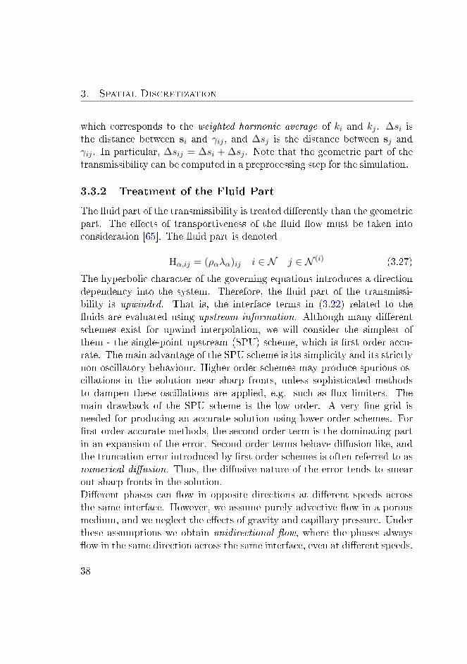
which corresponds to the weighted harmonic average of ki and kj . ∆si isthe distance between si and γij , and ∆sj is the distance between sj andγij . In particular, ∆sij = ∆si + ∆sj . Note that the geometric part of thetransmissibility can be computed in a preprocessing step for the simulation.
3.3.2 Treatment of the Fluid Part
The uid part of the transmissibility is treated dierently than the geometricpart. The eects of transportiveness of the uid ow must be taken intoconsideration [65]. The uid part is denoted
Hα,ij = (ραλα)ij i ∈ N j ∈ N (i) (3.27)
The hyperbolic character of the governing equations introduces a directiondependency into the system. Therefore, the uid part of the transmissi-bility is upwinded. That is, the interface terms in (3.22) related to theuids are evaluated using upstream information. Although many dierentschemes exist for upwind interpolation, we will consider the simplest ofthem - the single-point upstream (SPU) scheme, which is rst order accu-rate. The main advantage of the SPU scheme is its simplicity and its strictlynon-oscillatory behaviour. Higher order schemes may produce spurious os-cillations in the solution near sharp fronts, unless sophisticated methodsto dampen these oscillations are applied, e.g. such as ux limiters. Themain drawback of the SPU scheme is the low order. A very ne grid isneeded for producing an accurate solution using lower order schemes. Forrst order accurate methods, the second order term is the dominating partin an expansion of the error. Second order terms behave diusion-like, andthe truncation error introduced by rst order schemes is often referred to asnumerical diusion. Thus, the diusive nature of the error tends to smearout sharp fronts in the solution.Dierent phases can ow in opposite directions at dierent speeds acrossthe same interface. However, we assume purely advective ow in a porousmedium, and we neglect the eects of gravity and capillary pressure. Underthese assumptions we obtain unidirectional ow, where the phases alwaysow in the same direction across the same interface, even at dierent speeds.
38
3.4. Dierential Equation Model
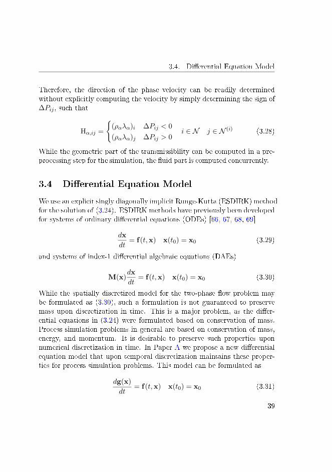
Therefore, the direction of the phase velocity can be readily determinedwithout explicitly computing the velocity by simply determining the sign of∆Pij , such that
Hα,ij =
(ραλα)i ∆Pij < 0
(ραλα)j ∆Pij > 0i ∈ N j ∈ N (i) (3.28)
While the geometric part of the transmissibility can be computed in a pre-processing step for the simulation, the uid part is computed concurrently.
3.4 Dierential Equation Model
We use an explicit singly diagonally implicit Runge-Kutta (ESDIRK) methodfor the solution of (3.24). ESDIRK methods have previously been developedfor systems of ordinary dierential equations (ODEs) [66, 67, 68, 69]
dx
dt= f(t,x) x(t0) = x0 (3.29)
and systems of index-1 dierential algebraic equations (DAEs)
M(x)dx
dt= f(t,x) x(t0) = x0 (3.30)
While the spatially discretized model for the two-phase ow problem maybe formulated as (3.30), such a formulation is not guaranteed to preservemass upon discretization in time. This is a major problem, as the dier-ential equations in (3.24) were formulated based on conservation of mass.Process simulation problems in general are based on conservation of mass,energy, and momentum. It is desirable to preserve such properties uponnumerical discretization in time. In Paper A we propose a new dierentialequation model that upon temporal discretization maintains these proper-ties for process simulation problems. This model can be formulated as
dg(x)
dt= f(t,x) x(t0) = x0 (3.31)
39

3. Spatial Discretization
in which x = x(t) are the system states, g(x) are the properties conserved,while the right-hand side function f(t,x) has the usual interpretation. Ingeneral, problems based on conservation of mass, energy, and momentum,can directly be formulated as the model (3.31). Upon discretization in timethis model preserves mass, energy, and momentum. This is not in generalthe case, if these problems are expressed as (3.30) using the chain rule, i.e.dg(x)dt = dg(x)
dxdxdt = M(x)dxdt with M(x) = dg(x)
dx . In Section 4.1.3 and 4.1.4we will formulate Runge-Kutta and ESDIRK methods for the purpose ofsolving dierential equation models that has the structure of (3.31).In the two-phase ow problem considered, x is a vector with pressure andwater saturation in each grid block, g(x) is a vector with oil and waterconcentrations in each grid block, and f(t,x) is a vector with the uxesof oil and water into each grid block plus any sources/sinks due to wells.Consequently, the spatially discretized model for two-phase ow (3.24) hasthe structure of (3.31).
3.5 Structure of the Jacobian Matrix
The application of ESDIRK methods for solution of the dierential equationmodel (3.31) involves the Jacobian of the residual form of this model. In par-ticular, for solution of the two-phase ow model considered using ESDIRKmethods, we must derive the Jacobian of (3.24) with respect to pressureand saturation. Since each grid block is associated with two equations (onefor oil and one for water) and two unknowns (pressure and saturation), theJacobian matrix will be of size 2N × 2N . Because the ux term in (3.24) isdependent on pressure and saturation in several grid blocks, we will use theux term to illustrate the non-zero structure of the Jacobian matrix. Thenet ux of oil and water into the ith grid block is
Fα,i =∑
j∈N (i)
(Υα∆P )ij i ∈ N (3.32)
Dene the vector
40
3.5. Structure of the Jacobian Matrix
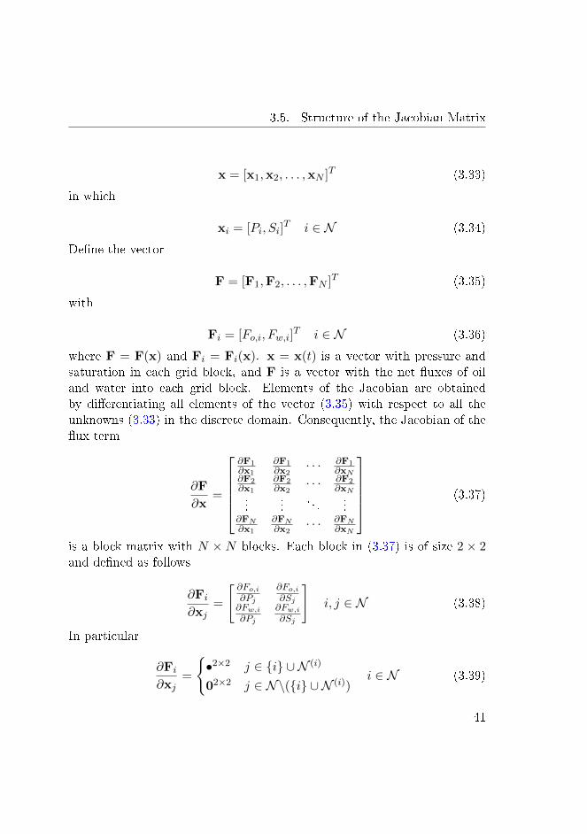
x = [x1,x2, . . . ,xN ]T (3.33)
in which
xi = [Pi, Si]T i ∈ N (3.34)
Dene the vector
F = [F1,F2, . . . ,FN ]T (3.35)
with
Fi = [Fo,i, Fw,i]T i ∈ N (3.36)
where F = F(x) and Fi = Fi(x). x = x(t) is a vector with pressure andsaturation in each grid block, and F is a vector with the net uxes of oiland water into each grid block. Elements of the Jacobian are obtainedby dierentiating all elements of the vector (3.35) with respect to all theunknowns (3.33) in the discrete domain. Consequently, the Jacobian of theux term
∂F
∂x=
∂F1∂x1
∂F1∂x2
· · · ∂F1∂xN
∂F2∂x1
∂F2∂x2
· · · ∂F2∂xN
......
. . ....
∂FN∂x1
∂FN∂x2
· · · ∂FN∂xN
(3.37)
is a block matrix with N ×N blocks. Each block in (3.37) is of size 2 × 2and dened as follows
∂Fi∂xj
=
[∂Fo,i∂Pj
∂Fo,i∂Sj
∂Fw,i∂Pj
∂Fw,i∂Sj
]i, j ∈ N (3.38)
In particular
∂Fi∂xj
=
•2×2 j ∈ i ∪ N (i)
02×2 j ∈ N\(i ∪ N (i))i ∈ N (3.39)
41
3. Spatial Discretization
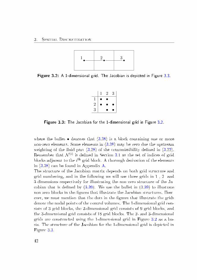
1 32
Figure 3.2: A 1-dimensional grid. The Jacobian is depicted in Figure 3.3.
1 2 3
1 • •2 • • •3 • •
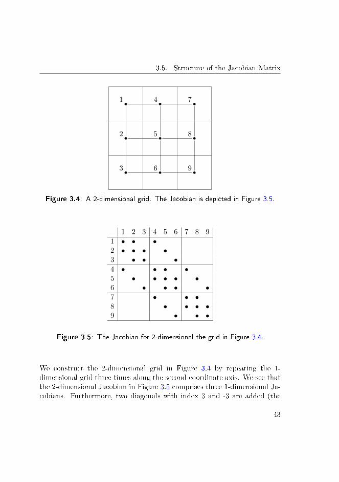
Figure 3.3: The Jacobian for the 1-dimensional grid in Figure 3.2.
where the bullet • denotes that (3.38) is a block containing one or morenon-zero elements. Some elements in (3.38) may be zero due the upstreamweighting of the uid part (3.28) of the transmissibility dened in (3.22).Remember that N (i) is dened in Section 3.1 as the set of indices of gridblocks adjacent to the ith grid block. A thorough derivation of the elementsin (3.38) can be found in Appendix A.The structure of the Jacobian matrix depends on both grid structure andgrid numbering, and in the following we will use three grids in 1-, 2- and3-dimensions respectively for illustrating the non-zero structure of the Ja-cobian that is dened by (3.39). We use the bullet in (3.39) to illustratenon-zero blocks in the gures that illustrate the Jacobian structures. How-ever, we must mention that the dots in the gures that illustrate the gridsdenote the nodal points of the control volumes. The 1-dimensional grid con-sists of 3 grid blocks, the 2-dimensional grid consists of 9 grid blocks, andthe 3-dimensional grid consists of 18 grid blocks. The 2- and 3-dimensionalgrids are constructed using the 1-dimensional grid in Figure 3.2 as a ba-sis. The structure of the Jacobian for the 1-dimensional grid is depicted inFigure 3.3.
42
3.5. Structure of the Jacobian Matrix
1 74
2
3
5
6
8
9
Figure 3.4: A 2-dimensional grid. The Jacobian is depicted in Figure 3.5.
1 2 3 4 5 6 7 8 9
1 • • •2 • • • •3 • • •4 • • • •5 • • • • •6 • • • •7 • • •8 • • • •9 • • •
Figure 3.5: The Jacobian for 2-dimensional the grid in Figure 3.4.
We construct the 2-dimensional grid in Figure 3.4 by repeating the 1-dimensional grid three times along the second coordinate axis. We see thatthe 2-dimensional Jacobian in Figure 3.5 comprises three 1-dimensional Ja-cobians. Furthermore, two diagonals with index 3 and -3 are added (the
43

3. Spatial Discretization
3i2
1
2
3
i1
i3 1
2
1 2
Figure 3.6: A 3-dimensional grid. The Jacobian is depicted in Figure 3.7.
main diagonal has index 0). These diagonals represent the new connectionsestablished by repeating the 1-dimensional grid. Let us use the grid blockwith index 2 in the 2-dimensional grid to illustrate the non-zero structuredened by (3.39): the grid is identied by the setN = 1, 2, 3, 4, 5, 6, 7, 8, 9,and N (2) = 1, 3, 5 is the set of grid blocks adjacent to the 2nd grid block.Implying that
∂F2
∂xj=
•2×2 j ∈ 1, 2, 3, 502×2 j ∈ 4, 6, 7, 8, 9
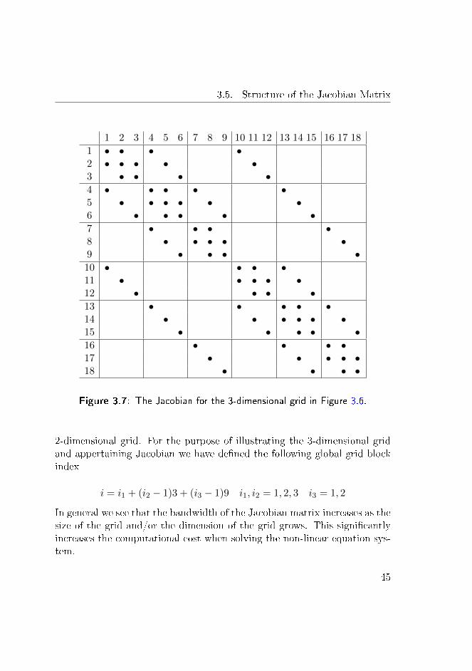
is the non-zero structure that describes the connections associated withblock number 2 in the 2-dimensional grid.The 3-dimensional grid in Figure 3.6 is constructed by repeating the 2-dimensional grid two times along the third coordinate axis. We see thatthe 3-dimensional Jacobian in Figure 3.7 comprises two 2-dimensional Ja-cobians. In addition, two diagonals with index 9 and -9 are added. Thesediagonals represent the new connections established by the repetition of the
44
3.5. Structure of the Jacobian Matrix
1 2 3 4 5 6 7 8 9 10 11 12 13 14 15 16 17 18
1 • • • •2 • • • • •3 • • • •4 • • • • •5 • • • • • •6 • • • • •7 • • • •8 • • • • •9 • • • •10 • • • •11 • • • • •12 • • • •13 • • • • •14 • • • • • •15 • • • • •16 • • • •17 • • • • •18 • • • •
Figure 3.7: The Jacobian for the 3-dimensional grid in Figure 3.6.
2-dimensional grid. For the purpose of illustrating the 3-dimensional gridand appertaining Jacobian we have dened the following global grid blockindex
i = i1 + (i2 − 1)3 + (i3 − 1)9 i1, i2 = 1, 2, 3 i3 = 1, 2
In general we see that the bandwidth of the Jacobian matrix increases as thesize of the grid and/or the dimension of the grid grows. This signicantlyincreases the computational cost when solving the non-linear equation sys-tem.
45
3. Spatial Discretization
The Jacobian matrices in Figure 3.3, 3.5 and 3.7 are not symmetric. Thisis because upwinding of the uid part of the transmissibility introducesasymmetry in the blocks (3.38). In general, the SPU scheme generatesasymmetric Jacobian matrices, which is a drawback in terms of solving thesystem of non-linear equations. However, assuming unidirectional ow andusing a sequential method for temporal discretization (see Section 4.1), areordering strategy can be applied [61]. The idea is to obtain a triangu-lar structure of the Jacobian. This may reduce the computational cost ofthe solution procedure. This adds another advantage to the SPU scheme,besides its simplicity and its non-oscillating behavior mentioned above.
3.6 Building the Dierential Equation Model and
the Jacobian Matrix
To solve the spatially discretized two-phase ow model using ESDIRKmeth-ods, we must interpret (3.24) so that we can formulate the problem in theform of (3.31). Dene the vector
C = [C1,C2, . . . ,CN ]T (3.40)
with the accumulation terms in (3.24), in which
Ci = [Co,i, Cw,i]T i ∈ N (3.41)
where C = C(x) and Ci = Ci(x). Dene the vector
Q = [Q1,Q2, . . . ,QN ]T (3.42)
with the source terms in (3.24), where
Qi = [Qo,i, Qw,i]T i ∈ N (3.43)
in which we dene Q = Q(x) and Qi = Qi(x). In Algorithm 3.6.1 we showhow to build the dierential equation model (3.31).As mentioned in Section 3.5, ESDIRK methods require the Jacobian of theresidual form of the dierential equation model (3.31). Therefore, we must
46
3.6. Building the Dierential Equation Model and the Jacobian Matrix
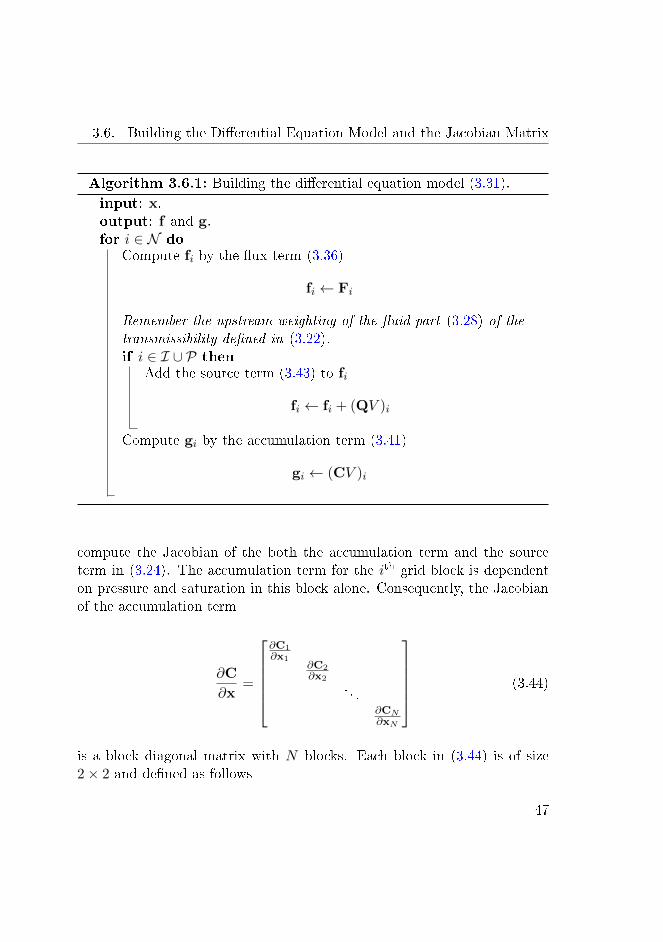
Algorithm 3.6.1: Building the dierential equation model (3.31).
input: x.output: f and g.for i ∈ N do
Compute fi by the ux term (3.36)
fi ← Fi
Remember the upstream weighting of the uid part (3.28) of thetransmissibility dened in (3.22).if i ∈ I ∪ P then
Add the source term (3.43) to fi
fi ← fi + (QV )i
Compute gi by the accumulation term (3.41)
gi ← (CV )i
compute the Jacobian of the both the accumulation term and the sourceterm in (3.24). The accumulation term for the ith grid block is dependenton pressure and saturation in this block alone. Consequently, the Jacobianof the accumulation term
∂C
∂x=
∂C1∂x1
∂C2∂x2
. . .∂CN∂xN
(3.44)
is a block diagonal matrix with N blocks. Each block in (3.44) is of size2× 2 and dened as follows
47

3. Spatial Discretization
Algorithm 3.6.2: Building the Jacobian matrix, ∂f∂x , of the right-
hand side and the Jacobian matrix, ∂g∂x , the left-hand side of the
dierential equation model (3.31).
input: x.output: ∂f
∂x and ∂g∂x .
for i ∈ N do
Compute ∂fi∂xi
by the Jacobian of the ux term (3.38)
∂fi∂xi← ∂Fi
∂xi
for j ∈ N (i) do
Compute ∂fi∂xj
by the Jacobian of the ux term (3.38)
∂fi∂xj← ∂Fi
∂xj
Remember the upstream weighting of the uid part (3.28) ofthe transmissibility dened in (3.22).if i ∈ I ∪ P then
Add the Jacobian of the source term (3.47) to ∂fi∂xi
∂fi∂xi← ∂fi
∂xi+∂Qi
∂xiVi
Compute ∂gi∂xi
by the Jacobian of the accumulation term (3.45)
∂gi∂xi← ∂Ci
∂xiVi
∂Ci
∂xi=
[∂Co,i∂Pi
∂Co,i∂Si
∂Cw,i∂Pi
∂Cw,i∂Si
]i ∈ N (3.45)
48
3.7. Summary
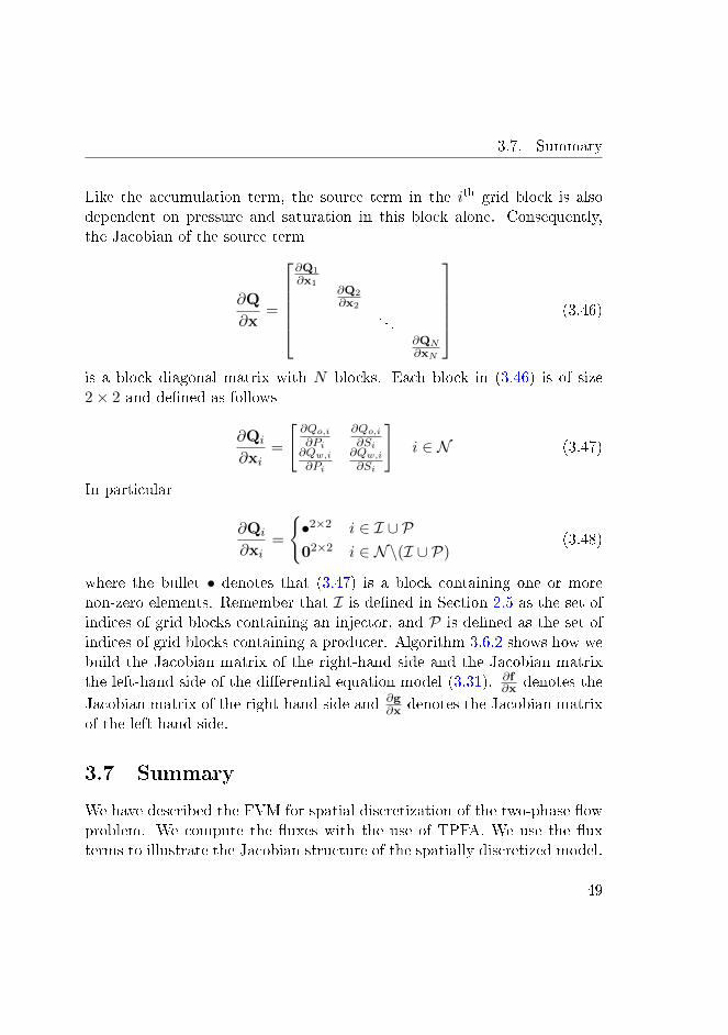
Like the accumulation term, the source term in the ith grid block is alsodependent on pressure and saturation in this block alone. Consequently,the Jacobian of the source term
∂Q
∂x=
∂Q1
∂x1∂Q2
∂x2
. . .∂QN∂xN
(3.46)
is a block diagonal matrix with N blocks. Each block in (3.46) is of size2× 2 and dened as follows
∂Qi
∂xi=
[∂Qo,i∂Pi
∂Qo,i∂Si
∂Qw,i∂Pi
∂Qw,i∂Si
]i ∈ N (3.47)
In particular
∂Qi
∂xi=
•2×2 i ∈ I ∪ P02×2 i ∈ N\(I ∪ P)
(3.48)
where the bullet • denotes that (3.47) is a block containing one or morenon-zero elements. Remember that I is dened in Section 2.5 as the set ofindices of grid blocks containing an injector, and P is dened as the set ofindices of grid blocks containing a producer. Algorithm 3.6.2 shows how webuild the Jacobian matrix of the right-hand side and the Jacobian matrixthe left-hand side of the dierential equation model (3.31). ∂f
∂x denotes the
Jacobian matrix of the right-hand side and ∂g∂x denotes the Jacobian matrix
of the left-hand side.
3.7 Summary
We have described the FVM for spatial discretization of the two-phase owproblem. We compute the uxes with the use of TPFA. We use the uxterms to illustrate the Jacobian structure of the spatially discretized model.
49
3. Spatial Discretization
We describe how to evaluate the interface transmissibilities: the geometricalpart of the transmissibilities is computed by a harmonic averaging of the ab-solute permeabilities, and the uid part is upwinded using the SPU scheme.We have presented a new dierential equation model, as proposed in Pa-per A. This model maintains the mass preserving property of the spatiallydiscretized two-phase ow problem upon temporal discretization. Manyprocess simulation problems are derived upon conservation of mass, energyand momentum, and therefore we may use (3.31) as a formulation for suchsystems in general.
50
CHAPTER 4Temporal Discretization
One of the key aspects in reservoir simulation is the integration of thedierential equation system constituting the model. The number and thetype of equations to be solved depend on the geological characteristics ofthe reservoir, the characteristics of the reservoir uids, and the oil recoveryprocess to be modelled. As a consequence of the system complexity it isnecessary to nd approximate solutions by numerical integration. Choosingthe appropriate method of integration involves deciding on factors such asthe order of the integration scheme, stability properties, and concern oncomputational eciency. In addition, a robust adaptive step size controlis essential to an ecient numerical integration. An adaptive step sizeselection aims to keep the error estimate of the solution bounded, i.e. closeto a user-specied tolerance by adjusting the size of the time step.The implicit pressure explicit saturation (IMPES) method [70, 71, 72], thesequential implicit method (SIM) [73, 74], and the implicit Euler method,normally referred to as the fully implicit method (FIM), are commonlyused for temporal discretization in reservoir simulation. The IMPES schemebenets from the explicit treatment of the saturation, the SIM benets fromthe sequential approach, while the FIM oers unconditionally stability in
51
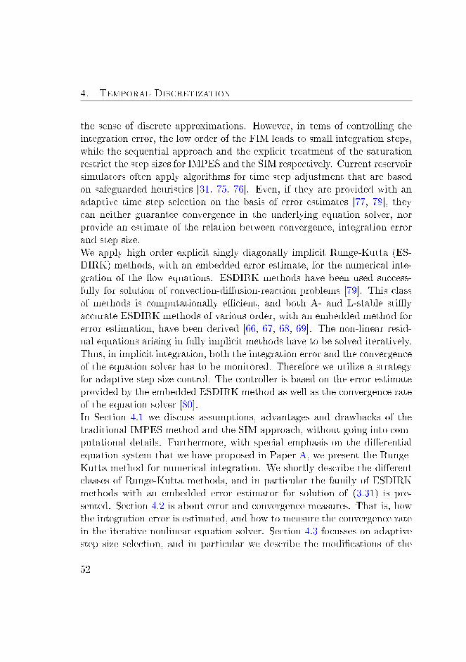
4. Temporal Discretization
the sense of discrete approximations. However, in tems of controlling theintegration error, the low order of the FIM leads to small integration steps,while the sequential approach and the explicit treatment of the saturationrestrict the step sizes for IMPES and the SIM respectively. Current reservoirsimulators often apply algorithms for time step adjustment that are basedon safeguarded heuristics [31, 75, 76]. Even, if they are provided with anadaptive time step selection on the basis of error estimates [77, 78], theycan neither guarantee convergence in the underlying equation solver, norprovide an estimate of the relation between convergence, integration errorand step size.We apply high order explicit singly diagonally implicit Runge-Kutta (ES-DIRK) methods, with an embedded error estimate, for the numerical inte-gration of the ow equations. ESDIRK methods have been used success-fully for solution of convection-diusion-reaction problems [79]. This classof methods is computationally ecient, and both A- and L-stable stiyaccurate ESDIRK methods of various order, with an embedded method forerror estimation, have been derived [66, 67, 68, 69]. The non-linear resid-ual equations arising in fully implicit methods have to be solved iteratively.Thus, in implicit integration, both the integration error and the convergenceof the equation solver has to be monitored. Therefore we utilize a strategyfor adaptive step size control. The controller is based on the error estimateprovided by the embedded ESDIRK method as well as the convergence rateof the equation solver [80].In Section 4.1 we discuss assumptions, advantages and drawbacks of thetraditional IMPES method and the SIM approach, without going into com-putational details. Furthermore, with special emphasis on the dierentialequation system that we have proposed in Paper A, we present the Runge-Kutta method for numerical integration. We shortly describe the dierentclasses of Runge-Kutta methods, and in particular the family of ESDIRKmethods with an embedded error estimator for solution of (3.31) is pre-sented. Section 4.2 is about error and convergence measures. That is, howthe integration error is estimated, and how to measure the convergence ratein the iterative nonlinear equation solver. Section 4.3 focusses on adaptivestep size selection, and in particular we describe the modications of the
52
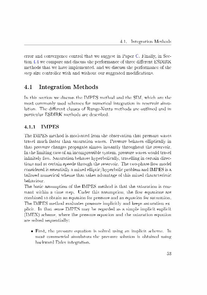
4.1. Integration Methods
error and convergence control that we suggest in Paper C. Finally, in Sec-tion 4.4 we compare and discuss the performance of three dierent ESDIRKmethods that we have implemented, and we discuss the performance of thestep size controller with and without our suggested modications.
4.1 Integration Methods
In this section we discuss the IMPES method and the SIM, which are themost commonly used schemes for numerical integration in reservoir simu-lation. The dierent classes of Runge-Kutta methods are outlined and inparticular ESDIRK methods are described.
4.1.1 IMPES
The IMPES method is motivated from the observation that pressure wavestravel much faster than saturation waves. Pressure behaves elliptically inthat pressure changes propagate almost instantly throughout the reservoir.In the limiting case of an incompressible system, pressure waves would travelinnitely fast. Saturation behaves hyperbolically, travelling in certain direc-tions and at certain speeds through the reservoir. The two-phase ow modelconsidered is essentially a mixed elliptic/hyperbolic problem and IMPES is atailored numerical scheme that takes advantage of this mixed characteristicbehaviour.The basic assumption of the IMPES method is that the saturation is con-stant within a time step. Under this assumption, the ow equations arecombined to obtain an equation for pressure and an equation for saturation.The IMPES method evaluates pressure implicitly and keeps saturation ex-plicit. In that sense IMPES may be regarded as a simple implicit-explicit(IMEX) scheme, where the pressure equation and the saturation equationare solved sequentially:
• First, the pressure equation is solved using an implicit scheme. Inmost commercial simulators the pressure solution is obtained usingbackward Euler integration.
53
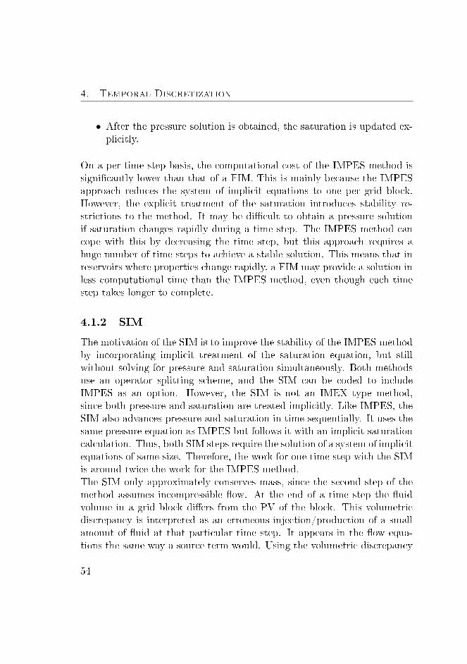
4. Temporal Discretization
• After the pressure solution is obtained, the saturation is updated ex-plicitly.
On a per time step basis, the computational cost of the IMPES method issignicantly lower than that of a FIM. This is mainly because the IMPESapproach reduces the system of implicit equations to one per grid block.However, the explicit treatment of the saturation introduces stability re-strictions to the method. It may be dicult to obtain a pressure solutionif saturation changes rapidly during a time step. The IMPES method cancope with this by decreasing the time step, but this approach requires ahuge number of time steps to achieve a stable solution. This means that inreservoirs where properties change rapidly, a FIM may provide a solution inless computational time than the IMPES method, even though each timestep takes longer to complete.
4.1.2 SIM
The motivation of the SIM is to improve the stability of the IMPES methodby incorporating implicit treatment of the saturation equation, but stillwithout solving for pressure and saturation simultaneously. Both methodsuse an operator splitting scheme, and the SIM can be coded to includeIMPES as an option. However, the SIM is not an IMEX type method,since both pressure and saturation are treated implicitly. Like IMPES, theSIM also advances pressure and saturation in time sequentially. It uses thesame pressure equation as IMPES but follows it with an implicit saturationcalculation. Thus, both SIM steps require the solution of a system of implicitequations of same size. Therefore, the work for one time step with the SIMis around twice the work for the IMPES method.The SIM only approximately conserves mass, since the second step of themethod assumes incompressible ow. At the end of a time step the uidvolume in a grid block diers from the PV of the block. This volumetricdiscrepancy is interpreted as an erroneous injection/production of a smallamount of uid at that particular time step. It appears in the ow equa-tions the same way a source term would. Using the volumetric discrepancy
54
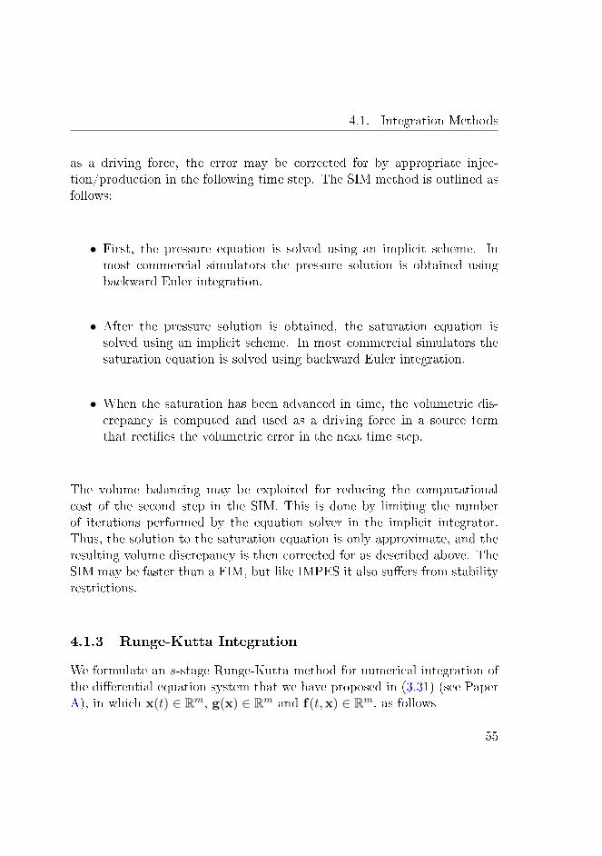
4.1. Integration Methods
as a driving force, the error may be corrected for by appropriate injec-tion/production in the following time step. The SIM method is outlined asfollows:
• First, the pressure equation is solved using an implicit scheme. Inmost commercial simulators the pressure solution is obtained usingbackward Euler integration.
• After the pressure solution is obtained, the saturation equation issolved using an implicit scheme. In most commercial simulators thesaturation equation is solved using backward Euler integration.
• When the saturation has been advanced in time, the volumetric dis-crepancy is computed and used as a driving force in a source termthat recties the volumetric error in the next time step.
The volume balancing may be exploited for reducing the computationalcost of the second step in the SIM. This is done by limiting the numberof iterations performed by the equation solver in the implicit integrator.Thus, the solution to the saturation equation is only approximate, and theresulting volume discrepancy is then corrected for as described above. TheSIM may be faster than a FIM, but like IMPES it also suers from stabilityrestrictions.
4.1.3 Runge-Kutta Integration
We formulate an s-stage Runge-Kutta method for numerical integration ofthe dierential equation system that we have proposed in (3.31) (see PaperA), in which x(t) ∈ Rm, g(x) ∈ Rm and f(t,x) ∈ Rm, as follows
55
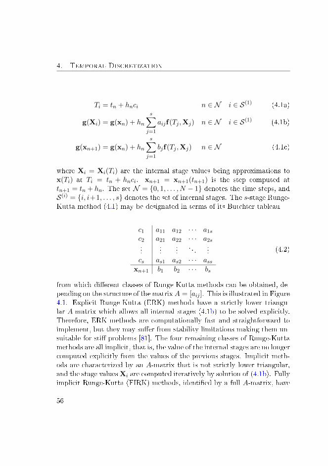
4. Temporal Discretization
Ti = tn + hnci n ∈ N i ∈ S(1) (4.1a)
g(Xi) = g(xn) + hn
s∑
j=1
aijf(Tj ,Xj) n ∈ N i ∈ S(1) (4.1b)
g(xn+1) = g(xn) + hn
s∑
j=1
bjf(Tj ,Xj) n ∈ N (4.1c)
where Xi = Xi(Ti) are the internal stage values being approximations tox(Ti) at Ti = tn + hnci. xn+1 = xn+1(tn+1) is the step computed attn+1 = tn + hn. The set N = 0, 1, . . . , N − 1 denotes the time steps, andS(i) = i, i+1, . . . , s denotes the set of internal stages. The s-stage Runge-Kutta method (4.1) may be designated in terms of its Butchter tableau
c1 a11 a12 · · · a1s
c2 a21 a22 · · · a2s...
......
. . ....
cs as1 as2 · · · assxn+1 b1 b2 · · · bs
(4.2)
from which dierent classes of Runge-Kutta methods can be obtained, de-pending on the structure of the matrixA = [aij ]. This is illustrated in Figure4.1. Explicit Runge-Kutta (ERK) methods have a strictly lower triangu-lar A-matrix which allows all internal stages (4.1b) to be solved explicitly.Therefore, ERK methods are computationally fast and straightforward toimplement, but they may suer from stability limitations making them un-suitable for sti problems [81]. The four remaining classes of Runge-Kuttamethods are all implicit, that is, the value of the internal stages are no longercomputed explicitly from the values of the previous stages. Implicit meth-ods are characterized by an A-matrix that is not strictly lower triangular,and the stage valuesXi are computed iteratively by solution of (4.1b). Fullyimplicit Runge-Kutta (FIRK) methods, identied by a full A-matrix, have
56
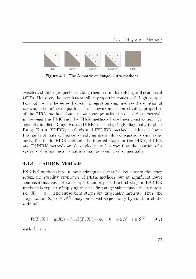
4.1. Integration Methods
0 0 0 00
γγ
γγ
γγ
γγ
γ
ERK DIRK SDIRK ESDIRK FIRK
Figure 4.1: The A-matrix of Runge-Kutta methods.
excellent stability properties making them usefull for solving sti systems ofODEs. However, the excellent stability properties comes with high compu-tational cost in the sense that each integration step involves the solution ofms coupled nonlinear equations. To achieve some of the stability propertiesof the FIRK methods but at lower computational cost, various methodsin between the ERK and the FIRK methods have been constructed. Di-agonally implicit Runge-Kutta (DIRK) methods, singly diagonally implicitRunge-Kutta (SDIRK) methods and ESDIRK methods all have a lowertriangular A-matrix. Instead of solving ms nonlinear equations simultane-ously, like in the FIRK method, the internal stages in the DIRK, SDIRKand ESDIRK methods are decoupled in such a way that the solution of ssystems of m nonlinear equations may be conducted sequentially.
4.1.4 ESDIRK Methods
ESDIRK methods have a lower triangular A-matrix. By construction theyretain the stability properties of FIRK methods but at signicant lowercomputational cost. Because c1 = 0 and a11 = 0 the rst stage in ESDIRKmethods is explicitly implying that the rst stage value equals the last step,i.e. X1 = xn. The subsequent stages are diagonally implicit. Thus, thestage values Xi, i ∈ S(2), may be solved sequentially by solution of theresidual
R(Ti,Xi) = g(Xi)− hnγf(Ti,Xi)−ψi = 0 n ∈ N i ∈ S(2) (4.3)
with the term
57
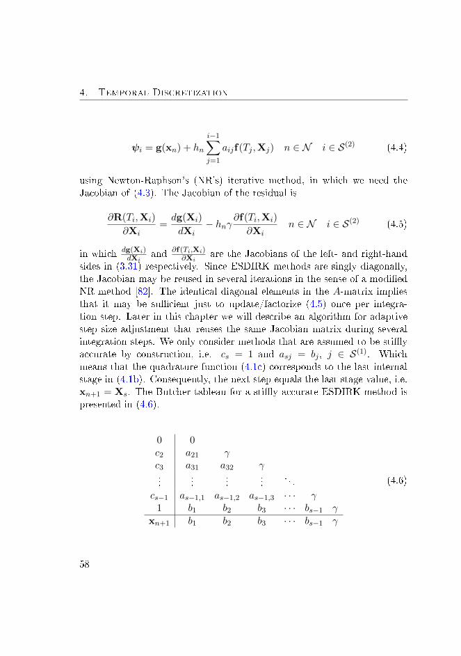
4. Temporal Discretization
ψi = g(xn) + hn
i−1∑
j=1
aijf(Tj ,Xj) n ∈ N i ∈ S(2) (4.4)
using Newton-Raphson's (NR's) iterative method, in which we need theJacobian of (4.3). The Jacobian of the residual is
∂R(Ti,Xi)
∂Xi=dg(Xi)
dXi− hnγ
∂f(Ti,Xi)
∂Xin ∈ N i ∈ S(2) (4.5)
in which dg(Xi)dXi
and ∂f(Ti,Xi)∂Xi
are the Jacobians of the left- and right-handsides in (3.31) respectively. Since ESDIRK methods are singly diagonally,the Jacobian may be reused in several iterations in the sense of a modiedNR method [82]. The identical diagonal elements in the A-matrix impliesthat it may be sucient just to update/factorize (4.5) once per integra-tion step. Later in this chapter we will describe an algorithm for adaptivestep size adjustment that reuses the same Jacobian matrix during severalintegration steps. We only consider methods that are assumed to be stiyaccurate by construction, i.e. cs = 1 and asj = bj , j ∈ S(1). Whichmeans that the quadrature function (4.1c) corresponds to the last internalstage in (4.1b). Consequently, the next step equals the last stage value, i.e.xn+1 = Xs. The Butcher tableau for a stiy accurate ESDIRK method ispresented in (4.6).
0 0c2 a21 γc3 a31 a32 γ...
......
.... . .
cs−1 as−1,1 as−1,2 as−1,3 · · · γ1 b1 b2 b3 · · · bs−1 γ
xn+1 b1 b2 b3 · · · bs−1 γ
(4.6)
58
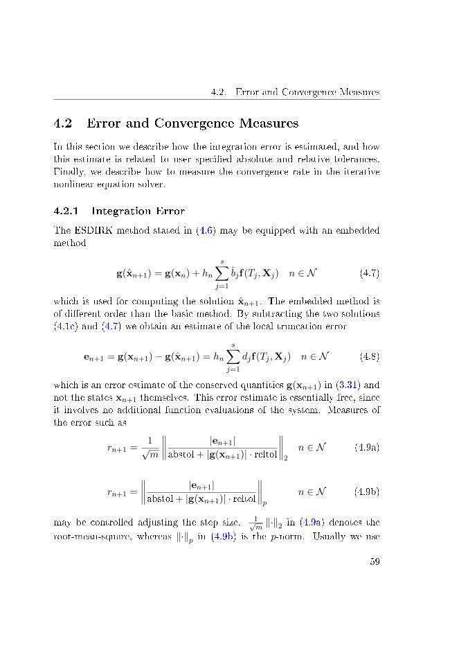
4.2. Error and Convergence Measures
4.2 Error and Convergence Measures
In this section we describe how the integration error is estimated, and howthis estimate is related to user specied absolute and relative tolerances.Finally, we describe how to measure the convergence rate in the iterativenonlinear equation solver.
4.2.1 Integration Error
The ESDIRK method stated in (4.6) may be equipped with an embeddedmethod
g(xn+1) = g(xn) + hn
s∑
j=1
bjf(Tj ,Xj) n ∈ N (4.7)
which is used for computing the solution xn+1. The embedded method isof dierent order than the basic method. By subtracting the two solutions(4.1c) and (4.7) we obtain an estimate of the local truncation error
en+1 = g(xn+1)− g(xn+1) = hn
s∑
j=1
djf(Tj ,Xj) n ∈ N (4.8)
which is an error estimate of the conserved quantities g(xn+1) in (3.31) andnot the states xn+1 themselves. This error estimate is essentially free, sinceit involves no additional function evaluations of the system. Measures ofthe error such as
rn+1 =1√m
∥∥∥∥|en+1|
abstol + |g(xn+1)| · reltol
∥∥∥∥2
n ∈ N (4.9a)
rn+1 =
∥∥∥∥|en+1|
abstol + |g(xn+1)| · reltol
∥∥∥∥p
n ∈ N (4.9b)
may be controlled adjusting the step size. 1√m‖·‖2 in (4.9a) denotes the
root-mean-square, whereas ‖·‖p in (4.9b) is the p-norm. Usually we use
59
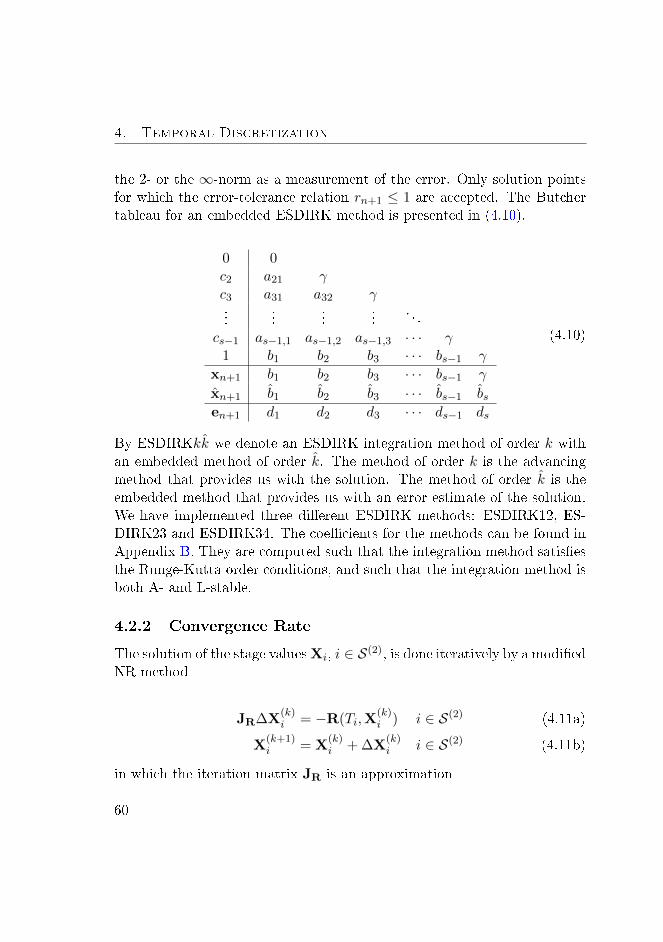
4. Temporal Discretization
the 2- or the ∞-norm as a measurement of the error. Only solution pointsfor which the error-tolerance relation rn+1 ≤ 1 are accepted. The Butchertableau for an embedded ESDIRK method is presented in (4.10).
0 0c2 a21 γc3 a31 a32 γ...
......
.... . .
cs−1 as−1,1 as−1,2 as−1,3 · · · γ1 b1 b2 b3 · · · bs−1 γ
xn+1 b1 b2 b3 · · · bs−1 γ
xn+1 b1 b2 b3 · · · bs−1 bsen+1 d1 d2 d3 · · · ds−1 ds
(4.10)
By ESDIRKkk we denote an ESDIRK integration method of order k withan embedded method of order k. The method of order k is the advancingmethod that provides us with the solution. The method of order k is theembedded method that provides us with an error estimate of the solution.We have implemented three dierent ESDIRK methods: ESDIRK12, ES-DIRK23 and ESDIRK34. The coecients for the methods can be found inAppendix B. They are computed such that the integration method satisesthe Runge-Kutta order conditions, and such that the integration method isboth A- and L-stable.
4.2.2 Convergence Rate
The solution of the stage valuesXi, i ∈ S(2), is done iteratively by a modiedNR method
JR∆X(k)i = −R(Ti,X
(k)i ) i ∈ S(2) (4.11a)
X(k+1)i = X
(k)i + ∆X
(k)i i ∈ S(2) (4.11b)
in which the iteration matrix JR is an approximation
60
4.2. Error and Convergence Measures
JR ≈∂R(Ti,X
(k)i )
∂X(k)i
(4.12)
to the Jacobian (4.5) of the residual (4.3). We solve the linear equationsystem (4.11a) with a direct method. We use sparse LU-factorizations,because the Jacobian is nonsymmetric, see Section 3.5. The controller needsto supervise the equation solver and answer questions like: when should theJacobian be evaluated/factorized, and what restrictions should be put onthe step size to ensure good convergence? To help answer these questions,the convergence rate of the NR solver is monitored and measured. Forreasons of robustness, the convergence rate is measured by the residuals[83]
α = maxi,k
r(k)R,i
r(k−1)R,i
i ∈ S(2) (4.13)
in which the iteration error of the kth iteration is computed as the followingresidual-tolerance relation
r(k)R,i =
1√m
∥∥∥∥∥|R(Ti,X
(k)i )|
abstol + |g(X(k)i )| · reltol
∥∥∥∥∥2
i ∈ S(2) (4.14a)
r(k)R,i =
∥∥∥∥∥|R(Ti,X
(k)i )|
abstol + |g(X(k)i )| · reltol
∥∥∥∥∥p
i ∈ S(2) (4.14b)
using the same componentwise absolute and relative error tolerances as in(4.9). For robustness the iteration sequence should be contractive. If forsome k during the iterations α ≥ 1 the iteration sequence is terminated. Inthe event of termination either a Jacobian update/factorization is called foror the step size is restricted. In case of convergence, the equation solver is
successfully stopped when r(k)R,i ≤ τ . The choice of τ aects the eciency
of the controller [81]. We must choose τ 1, such that the error estimate
61
4. Temporal Discretization
will not be dominated by the contribution from the iteration error. A largevalue of τ may lead to one or more large components in the integrationerror, with too many rejected steps as a result. We have chosen τ = 0.1as a compromise between robustness and computational speed. In Algo-rithm 4.2.1 we present an outline of the ESDIRK integration method usingadaptive step size control.
4.3 Step Size Selection
Adaptive step size selection is, in essence, a control problem, with the ob-jective of producing numerical solutions for which the integration error (4.8)is kept within a certain tolerance. We have modied and implemented analgorithm for adaptive step size selection originally developed by [80]. Ourmodications concern: the error control, the convergence control, and asimplication of the algorithm in general. In this section we briey describethe key parts of the control strategy and the modications of the error andconvergence control that we propose. The motivation for our modicationsand the modied version of the algorithm can be found in Paper C. Beforewe continue let us mention that we have two possible candidates for thenext step size, hn+1. The rst candidate, hr, is based on an estimate of theintegration error. The second candidate, hα, is based on the convergencerate in the equation solver. This is seen in Figure 4.2, depicting a blockdiagram of the modied control strategy.
4.3.1 Error Control
The original algorithm uses two rules for controlling the error of the so-lution: the asymptotic rule for step size adjustment, and a proportionalintegral (PI) step size controller. We start by describing the rules above,and nally the modication that we propose. The asymptotic rule for stepsize selection, which is the conventional control law that is commonly im-plemented in ODE solvers, is as follows
62

4.3. Step Size Selection
Algorithm 4.2.1: ESDIRK integration using adaptive step size control.
input: x0, t0 and tf (the nal time).output: xn+1N−1
n=0 .while tn < tf do
Assign
T1 ← tn
X1 ← xn
for i ∈ S(2) doCompute the stage value time Ti by (4.1a).Assign
Xi ← xn
Compute the residual R(Ti,Xi) by (4.3).while iterations not converged do
Compute the stage value Xi by solution of (4.11).
Compute the residual-tolerance relation r(k)R,i by (4.14).
Compute the convergence rate α by (4.13).
Assign
tn+1 ← Ts
xn+1 ← Xs
Compute the error-tolerance relation rn+1 by (4.9).Apply step size control cf. Algorithm 4.3.3.
hr =
(ε
rn+1
)1/k
hn n ∈ N (4.15)
The asymptotic step size selection rule uses only current information aboutthe step size and the error in order to achieve rn+1 = ε. Occasionally,
63
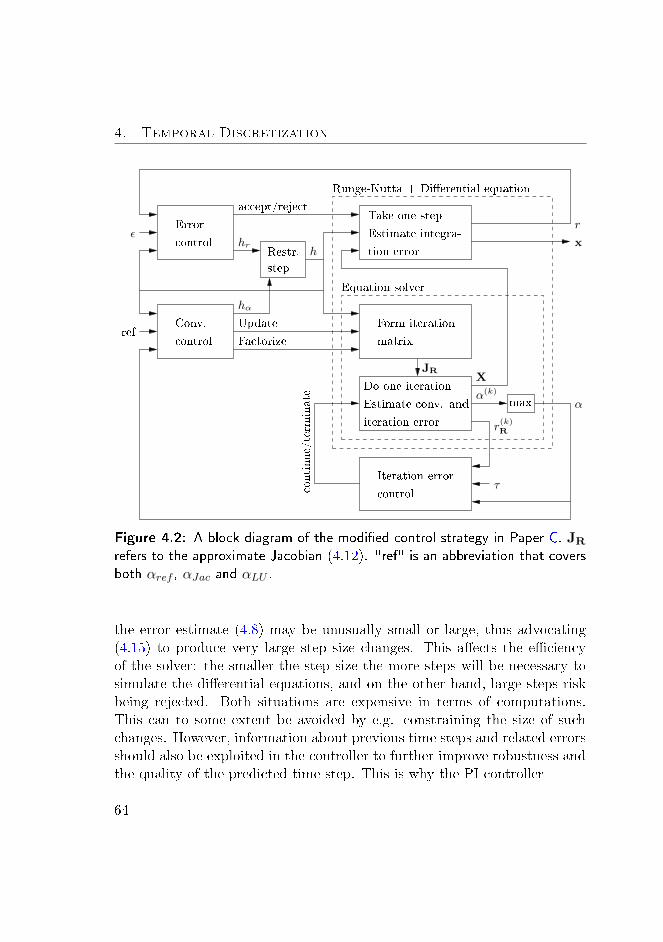
4. Temporal Discretization
Do one iteration
continue/term
inate
Update
accept/reject
Factorize
τ
α
x
JR
α(k)
Equation solver
iteration error
ε
Estimate conv. and
ref
r
X
Runge-Kutta + Dierential equation
hα
Iteration error
control
hrh
r(k)R
Conv.
control
control
ErrorTake one step
Estimate integra-
tion errorRestr.
step
max
Form iteration
matrix
Figure 4.2: A block diagram of the modied control strategy in Paper C. JR
refers to the approximate Jacobian (4.12). "ref" is an abbreviation that coversboth αref , αJac and αLU .
the error estimate (4.8) may be unusually small or large, thus advocating(4.15) to produce very large step size changes. This aects the eciencyof the solver: the smaller the step size the more steps will be necessary tosimulate the dierential equations, and on the other hand, large steps riskbeing rejected. Both situations are expensive in terms of computations.This can to some extent be avoided by e.g. constraining the size of suchchanges. However, information about previous time steps and related errorsshould also be exploited in the controller to further improve robustness andthe quality of the predicted time step. This is why the PI controller
64
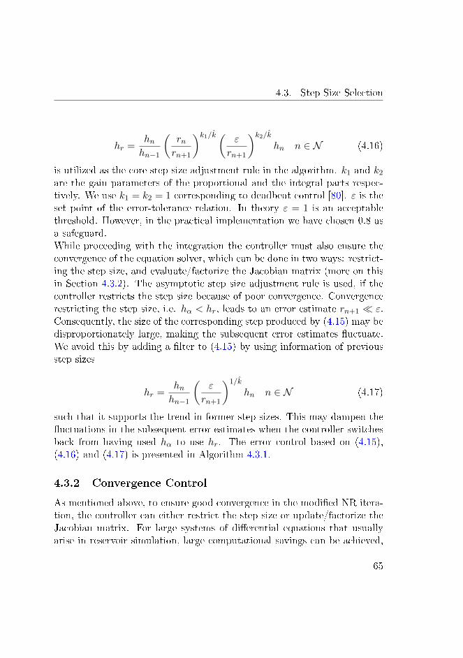
4.3. Step Size Selection
hr =hnhn−1
(rnrn+1
)k1/k ( ε
rn+1
)k2/khn n ∈ N (4.16)
is utilized as the core step size adjustment rule in the algorithm. k1 and k2
are the gain parameters of the proportional and the integral parts respec-tively. We use k1 = k2 = 1 corresponding to deadbeat control [80]. ε is theset point of the error-tolerance relation. In theory ε = 1 is an acceptablethreshold. However, in the practical implementation we have chosen 0.8 asa safeguard.While proceeding with the integration the controller must also ensure theconvergence of the equation solver, which can be done in two ways: restrict-ing the step size, and evaluate/factorize the Jacobian matrix (more on thisin Section 4.3.2). The asymptotic step size adjustment rule is used, if thecontroller restricts the step size because of poor convergence. Convergencerestricting the step size, i.e. hα < hr, leads to an error estimate rn+1 ε.Consequently, the size of the corresponding step produced by (4.15) may bedisproportionately large, making the subsequent error estimates uctuate.We avoid this by adding a lter to (4.15) by using information of previousstep sizes
hr =hnhn−1
(ε
rn+1
)1/k
hn n ∈ N (4.17)
such that it supports the trend in former step sizes. This may dampen theuctuations in the subsequent error estimates when the controller switchesback from having used hα to use hr. The error control based on (4.15),(4.16) and (4.17) is presented in Algorithm 4.3.1.
4.3.2 Convergence Control
As mentioned above, to ensure good convergence in the modied NR itera-tion, the controller can either restrict the step size or update/factorize theJacobian matrix. For large systems of dierential equations that usuallyarise in reservoir simulation, large computational savings can be achieved,
65
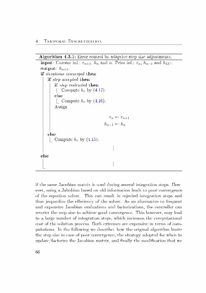
4. Temporal Discretization
Algorithm 4.3.1: Error control by adaptive step size adjustments.
input: Current inf.: rn+1, hn and α. Prior inf.: rn, hn−1 and hLU .output: hn+1.if iterations converged then
if step accepted then
if step restricted thenCompute hr by (4.17).
elseCompute hr by (4.16).
Assign
rn ← rn+1
hn−1 ← hn
elseCompute hr by (4.15).
...
else...
if the same Jacobian matrix is used during several integration steps. How-ever, using a Jabobian based on old information leads to poor convergenceof the equation solver. This can result in rejected integration steps andthus jeopardize the eeciency of the solver. As an alternative to frequentand expensive Jacobian evaluations and factorizations, the controller canrestrict the step size to achieve good convergence. This however, may leadto a large number of integration steps, which increases the computationalcost of the solution process. Both extremes are expensive in terms of com-putations. In the following we describe: how the original algorithm limitsthe step size in case of poor convergence, the strategy adopted for when toupdate/factorize the Jacobian matrix, and nally the modication that we
66

4.3. Step Size Selection
suggest.The Jacobian is not evaluated at every integration step. Thus, the Jacobianis an approximation calculated at some solution point. The approximationwill deteriorate gradually for the subsequent steps, but at least we expectgood convergence at this point. However, in some cases the distance betweenthe stage points may be too large, and the convergence will be poor althoughthe Jacobian is based on current data. In this case, the only option is todecrease the distance between the stage points by reducing the step size. Ifconvergence is poor, i.e. if α > αref the step size should be chosen as
hα =αrefα
hn n ∈ N (4.18)
to achieve α = αref in the next step [80]. The main purpose of the steplength control is to comply with the accuracy requirement. Therefore, thestep size suggested by (4.18) has to be coordinated with one from the errorcontrol. Consequently, if poor convergence is observed in spite of a Jacobianbased on current data, the step size is implemented as
hn+1 = min(hr, hα) n ∈ N (4.19)
restricting the step size by convergence if hα < hr. Slow convergence inthe equation solver can to some extend be avoided by step size reductions.However, considering (4.5) we see that a step size change may imply afactorization of the Jacobian matrix. In some cases however, it is not enoughsimply to factorize the Jacobian matrix. To ensure convergence, it may benecessary to both evaluate and factorize the Jacobian. This implies, thatwe need a factorization/evaluation strategy for the Jacobian matrix. Bymonitoring the relative step size change since the last factorization wasdone, the following relation
|hn+1 − hLU |/hLU > αLU n ∈ N (4.20)
is used as a rule for when a factorization should be applied. The strategytries to anticipate possible convergence failures and factorizes the Jacobian,if a planned step size change is likely to jeopardize convergence. Should poor
67

4. Temporal Discretization
convergence be experienced despite of a recent factorization, the followingrule
α− |hn+1 − hLU |/hLU > αJac n ∈ N (4.21)
determines whether the Jacobian should be updated instead [84]. Thisstrategy both monitors the convergence rate and balances the amount ofcomputational time spent on Jacobian updates and factorizations versusfunction evaluations in the equation solver.When convergence restricts the step size, i.e. hα < hr, any value of α thatdeviates from αref will be brought to the reference in one step. This may bea too agressive strategy, making the subsequent error estimates uctuate.We prevent this to some extent by using (4.17) instead of (4.15) for thesubsequent calculation of hr. In addition, we modify (4.18) to
hα =(αref
α
)1/khn n ∈ N (4.22)
such that the convergence restriction becomes less agressive. Thus, we mayavoid that the corresponding error estimate deviates too much, and we get asmoother transition in the error estimate when the controller switches backfrom having used hα to use hr.The eciency of an implicit integration method depends highly on the con-vergence in the equation solver, i.e. the value of the set point αref . In mostcases, any value 0.2 < αref < 0.5 is acceptable as reference for the conver-gence rate, with robustness favoring the lower values. We use αref = 0.4in our implementation [85, 80]. For the administration of the Jacobian, wehave chosen αJac = 0.2 and αLU = 0.2. For the two-phase ow problem,this choice seems like a good balance between the computational load of theequation solver in comparison to the computational cost of Jacobian eval-uations/factorizations. With these settings we try to minimize the totalcomputational time spent on the solution process. The maximum numberof iterations allowed in the equation solver is 10. The convergence controlbased on (4.19), (4.20), (4.21) and (4.22) is presented in Algorithm 4.3.2.
68
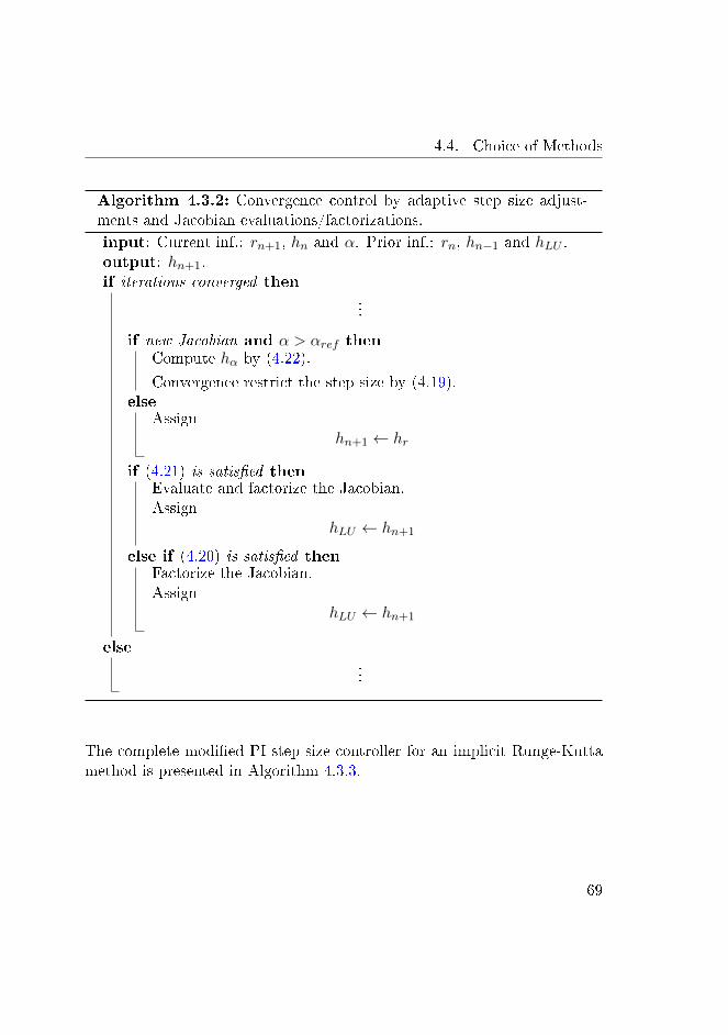
4.4. Choice of Methods
Algorithm 4.3.2: Convergence control by adaptive step size adjust-ments and Jacobian evaluations/factorizations.
input: Current inf.: rn+1, hn and α. Prior inf.: rn, hn−1 and hLU .output: hn+1.if iterations converged then
...
if new Jacobian and α > αref thenCompute hα by (4.22).
Convergence restrict the step size by (4.19).else
Assignhn+1 ← hr
if (4.21) is satised thenEvaluate and factorize the Jacobian.Assign
hLU ← hn+1
else if (4.20) is satised thenFactorize the Jacobian.Assign
hLU ← hn+1
else...
The complete modied PI step size controller for an implicit Runge-Kuttamethod is presented in Algorithm 4.3.3.
69
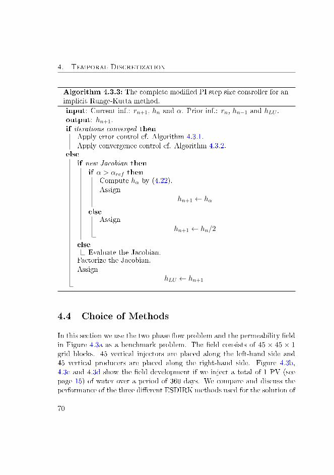
4. Temporal Discretization
Algorithm 4.3.3: The complete modied PI step size controller for animplicit Runge-Kutta method.
input: Current inf.: rn+1, hn and α. Prior inf.: rn, hn−1 and hLU .output: hn+1.if iterations converged then
Apply error control cf. Algorithm 4.3.1.Apply convergence control cf. Algorithm 4.3.2.
else
if new Jacobian then
if α > αref thenCompute hα by (4.22).Assign
hn+1 ← hα
elseAssign
hn+1 ← hn/2
elseEvaluate the Jacobian.
Factorize the Jacobian.Assign
hLU ← hn+1
4.4 Choice of Methods
In this section we use the two-phase ow problem and the permeability eldin Figure 4.3a as a benchmark problem. The eld consists of 45 × 45 × 1grid blocks. 45 vertical injectors are placed along the left-hand side and45 vertical producers are placed along the right-hand side. Figure 4.3b,4.3c and 4.3d show the eld development if we inject a total of 1 PV (seepage 15) of water over a period of 360 days. We compare and discuss theperformance of the three dierent ESDIRK methods used for the solution of
70
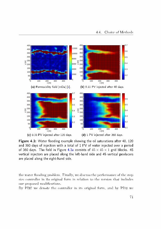
4.4. Choice of Methods
x [m]
y [m
]
0 100 200 300 4000
50
100
150
200
250
300
350
400
450
0
2000
4000
6000
8000
10000
12000
(a) Permeability eld [mDa] [1].
x [m]
y [m
]
0 100 200 300 4000
50
100
150
200
250
300
350
400
450
0.2
0.3
0.4
0.5
0.6
0.7
(b) 0.11 PV injected after 40 days.
x [m]
y [m
]
0 100 200 300 4000
50
100
150
200
250
300
350
400
450
0.2
0.3
0.4
0.5
0.6
0.7
(c) 0.33 PV injected after 120 days.
x [m]
y [m
]
0 100 200 300 4000
50
100
150
200
250
300
350
400
450
0.1
0.2
0.3
0.4
0.5
0.6
(d) 1 PV injected after 360 days.
Figure 4.3: Water ooding example showing the oil saturations after 40, 120and 360 days of injection with a total of 1 PV of water injected over a periodof 360 days. The eld in Figure 4.3a consists of 45 × 45 × 1 grid blocks. 45vertical injectors are placed along the left-hand side and 45 vertical producersare placed along the right-hand side.
the water ooding problem. Finally, we discuss the performance of the stepsize controller in its original form in relation to the version that includesour proposed modications.By PI97 we denote the controller in its original form, and by PI10 we
71

4. Temporal Discretization
refer to the modied version (according to Paper C). For the work-precisiondiagrams we used a xed absolute tolerance of 10−8 and relative tolerancesin the range from 10−8 to 10−2. We denote these as signicant digits (SDs),such that SD = 4 corresponds to a relative tolerance of 10−4. The numberof function evaluations, which are listed in the following, can be directlyequated with the number of iterations in the equation solver.
4.4.1 Choice of ESDIRK Methods
From the work-precision diagram in Figure 4.4a, we see that the total com-putational cost of ESDIRK12 increases in a more profound way than theother two methos. This is due to the small step sizes, which are necessaryfor the method in order to satisfy the required accuracy of the solution.This implies an increased workload of the equation solver when trying toretain (rR)ki ≤ τ . In addition, small step sizes lead to an increase in over-head time, which can be seen in Figure 4.4b. As can be seen in Figure 4.4cand Figure 4.4d, ESDIRK23 and ESDIRK34 are better at maintaining anappropriate distribution of the workload as the requirements in accuracy in-crease. Except for SD = 2, we can observe from the work-precision diagramof the three methods, that ESDIRK23 is overall the most computationallyecient method for temporal discretization of the two-phase ow problem.
4.4.2 Choice of step size Controller
The step size sequences for the PI97 and the PI10 controllers are depictedin Figure 4.5a and in Figure 4.5b respectively. It must be mentioned thatnStep, nFail and nSlow refer to the number of timesteps used in order toobtain the solution, the number of steps rejected by the error control, i.e.rn+1 > 1, and the amount of steps rejected because the maximum numberof iterations is reached. By comparing the performance of the two con-trollers, we see that fewer Jacobian evaluations/factorizations are requiredby the PI10 controller in the sense of maintaining good convergence in theequation solver. Thus fewer iterations are necessary in order to completethe integration. Because of the less aggressive step size change suggested by
72
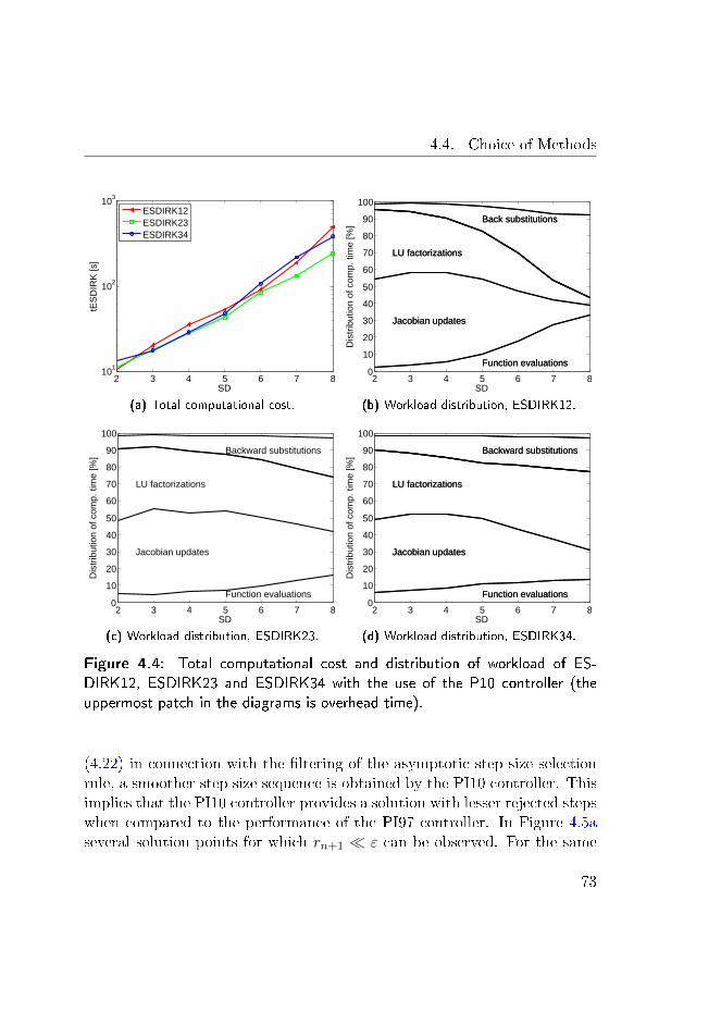
4.4. Choice of Methods
2 3 4 5 6 7 810
1
102
103
SD
tES
DIR
K [s
]
ESDIRK12ESDIRK23ESDIRK34
(a) Total computational cost.
2 3 4 5 6 7 80
10
20
30
40
50
60
70
80
90
100
SD
Dis
trib
utio
n of
com
p. ti
me
[%]
Function evaluations
Jacobian updates
LU factorizations
Back substitutions
Function evaluations
Jacobian updates
LU factorizations
Back substitutions
(b) Workload distribution, ESDIRK12.
2 3 4 5 6 7 80
10
20
30
40
50
60
70
80
90
100
SD
Dis
trib
utio
n of
com
p. ti
me
[%]
Function evaluations
Jacobian updates
LU factorizations
Backward substitutions
(c) Workload distribution, ESDIRK23.
2 3 4 5 6 7 80
10
20
30
40
50
60
70
80
90
100
SD
Dis
trib
utio
n of
com
p. ti
me
[%]
Function evaluations
Jacobian updates
LU factorizations
Backward substitutions
Function evaluations
Jacobian updates
LU factorizations
Backward substitutions
(d) Workload distribution, ESDIRK34.
Figure 4.4: Total computational cost and distribution of workload of ES-DIRK12, ESDIRK23 and ESDIRK34 with the use of the P10 controller (theuppermost patch in the diagrams is overhead time).
(4.22) in connection with the ltering of the asymptotic step size selectionrule, a smoother step size sequence is obtained by the PI10 controller. Thisimplies that the PI10 controller provides a solution with lesser rejected stepswhen compared to the performance of the PI97 controller. In Figure 4.5aseveral solution points for which rn+1 ε can be observed. For the same
73
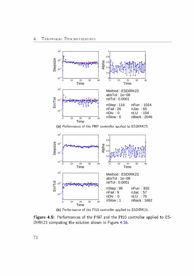
4. Temporal Discretization
0 10 20 30 4010
−2
10−1
100
101
Time
Ste
psiz
e
0 10 20 30 40
10−2
100
102
Time
Err
/Tol
0 10 20 30 400
0.2
0.4
0.6
0.8
1
Time
Alp
ha
Method : ESDIRK23absTol : 1e−08relTol : 0.0001
nStep : 116nFail : 26nDiv : 0nSlow : 6
nFun : 1024nJac : 65nLU : 104nBack : 2046
(a) Performance of the PI97 controller applied to ESDIRK23.
0 10 20 30 4010
−2
10−1
100
101
Time
Ste
psiz
e
0 10 20 30 40
10−2
100
102
Time
Err
/Tol
0 10 20 30 400
0.2
0.4
0.6
0.8
1
Time
Alp
ha
Method : ESDIRK23absTol : 1e−08relTol : 0.0001
nStep : 96nFail : 9nDiv : 0nSlow : 1
nFun : 832nJac : 57nLU : 76nBack : 1662
(b) Performance of the PI10 controller applied to ESDIRK23.
Figure 4.5: Performances of the PI97 and the PI10 controller applied to ES-DIRK23 computing the solution shown in Figure 4.3b.
74
4.5. Summary
solution points the corresponding step sizes are small. Due to the ability of(4.22) to increase the step size as well, this behaviour is only to a lesser ex-tent observed in Figure 4.5b. Hence the PI10 controller may produce largerstep sizes in situations where the integration error and the convergence rateare below their respective set points. In Figure 4.6 we compare the compu-tational cost of the two controllers. We notice, that in comparison to thePI97 controller, a better performance is obtained in the range from 2 to 5SDs for the PI10 controller. The requirements for the accuracy in reservoirsimulation is often within the range mentioned above. Therefore, we pro-pose the use of the modied step length controller in Paper C for implicitintegration of dynamic systems such as the two-phase ow problem.
4.5 Summary
We have described the most commonly used schemes for temporal discretiza-tion in reservoir simulation: the FIM, the IMPES method and the SIM.With special emphasies on the dierential equation system (3.31) that wepropose in Paper A, we have presented three dierent ESDIRK methodswith an embedded error estimator: ESDIRK12, ESDIRK23 and ESDIRK34.All three methods are both A- and L-stable, as well as stiy accurate. Wehave described an adaptive step size control that is based on the embed-ded error estimator. In particular, we have described the modications ofthe error and convergence control that we suggest in Paper C. Finally, wehave discussed the performance of the three ESDIRK methods, and theperformance of the step size controller both in its original form and withthe modications that we suggest.
75

4. Temporal Discretization
2 3 4 5 6 7 810
1
102
103
SD
tES
DIR
K12
[s]
PI97PI10
(a) Total computational cost, ESDIRK12.
2 3 4 5 6 7 810
1
102
103
SD
tES
DIR
K23
[s]
PI97PI10
(b) Computational cost of ESDIRK23.
2 3 4 5 6 7 810
1
102
103
SD
tES
DIR
K34
[s]
PI97PI10
(c) Computational cost of ESDIRK34.
2 3 4 5 6 7 80.8
0.9
1
1.1
1.2
1.3
SD
Rel
ativ
e sp
eedu
p
ESDIRK12ESDIRK23ESDIRK34
(d) Relative speedup, tPI10tPI97
.
Figure 4.6: Comparison of the PI97 and the PI10 controller separately usedwith ESDIRK12, ESDIRK 23 and ESDIRK34.
76

CHAPTER 5Production Optimization
Petroleum reservoirs are subsurface formations of porous rocks with hy-drocarbons trapped in the pores. Initially, the reservoir pressure may besuciently large to push the uids to the production facilities. However,as the uids are produced the pressure declines and production reducesover time. When the natural pressure becomes insucient, the pressuremust be maintained articially by injection of water. Conventional tech-nologies for recovery leaves more than 50% of the oil in the reservoir. Wellswith adjustable downhole ow control devices coupled with modern con-trol technology oer the potential to increase the oil recovery signicantly.Optimal control of smart-wells have been introduced [1]. In these applica-tions, downhole sensor equipment and remotely controlled valves are usedin combination with large-scale subsurface ow models and gradient basedoptimization methods in a NMPC framework to increase the productionand economic value of an oil reservoir [15, 25, 13, 26, 19]. Wether the ob-jective is to maximize recovery or some nancial measure like net presentvalue (NPV), the increased production is achieved by manipulation of thewell rates and BHPs of the injection and production wells. The optimalwater injection rates and production well BHPs are computed by solution
77
5. Production Optimization
of a large-scale constrained optimal control problem.In this chapter, we focus on maximizing the economical value of an oil eldand describe the gradient based method to compute the optimal controlstrategy. The discrete-time optimal control problem can be solved usingsingle-shooting [86, 87], multiple-shooting [88, 89], and the simultaneousmethod [90, 91, 92]. Reservoir models are large-scale and the number ofstates are easily in the order of magnitude of 105-106 for realistic problems.Thus, we describe a single-shooting algorithm for solution of the non-linearconstrained optimal control problem. An ESDIRK method with an adaptivestep size control, see Chapter 4 and Paper C, is used for computationallyecient solution of the model. The gradients are eciently computed usingthe adjoint method [93, 36, 22, 37]. The constrained optimization is per-formed using quasi-Newton sequential quadratic programming (SQP) withline-search and modied BFGS approximations [94]. The adjoint equationsassociated with the integration scheme are solved by integrating backwardsin time. The necessary information for the adjoint computation is com-puted and stored during the forward solution of the model. The backwardadjoint computation assembles this information to compute the gradients[13]. With the use of the spatial discretization presented in Section 3.1 -3.2, we demonstrate the optimal control strategy using the 2-dimensionalwater ooding example presented in Chapter 2.The chapter is organized as follows. Section 5.1 states the general con-strained optimal control problem using the novel representation of the sys-tem dynamics that we propose in Section 3.4 and Paper A. The numericalmethods for the constrained optimal control problem are described in Sec-tion 5.2 - 5.4. Section 5.5 describes specic details related to the objectivefunction and the constraints for the water ooding production optimiza-tion problem. In this section we also describe the numerical case studyillustrating the optimization algorithm when applied to the water oodingproblem.
78
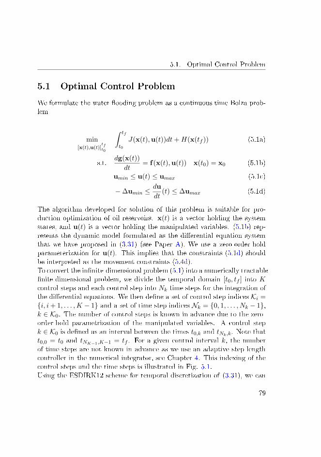
5.1. Optimal Control Problem
5.1 Optimal Control Problem
We formulate the water ooding problem as a continuous time Bolza prob-lem
min[x(t),u(t)]
tft0
∫ tf
t0
J(x(t),u(t))dt+H(x(tf )) (5.1a)
s.t.dg(x(t))
dt= f(x(t),u(t)) x(t0) = x0 (5.1b)
umin ≤ u(t) ≤ umax (5.1c)
−∆umin ≤du
dt(t) ≤ ∆umax (5.1d)
The algorithm developed for solution of this problem is suitable for pro-duction optimization of oil reservoirs. x(t) is a vector holding the systemstates, and u(t) is a vector holding the manipulated variables. (5.1b) rep-resents the dynamic model formulated as the dierential equation systemthat we have proposed in (3.31) (see Paper A). We use a zero-order-holdparameterization for u(t). This implies that the constraints (5.1d) shouldbe interpreted as the movement constraints (5.4d).To convert the innite-dimensional problem (5.1) into a numerically tractablenite-dimensional problem, we divide the temporal domain [t0, tf ] into Kcontrol steps and each control step into Nk time steps for the integration ofthe dierential equations. We then dene a set of control step indices Ki =i, i+ 1, . . . ,K − 1 and a set of time step indices Nk = 0, 1, . . . , Nk − 1,k ∈ K0. The number of control steps is known in advance due to the zero-order-hold parametrization of the manipulated variables. A control stepk ∈ K0 is dened as an interval between the times t0,k and tNk,k. Note thatt0,0 = t0 and tNK−1,K−1 = tf . For a given control interval k, the numberof time steps are not known in advance as we use an adaptive step lengthcontroller in the numerical integrator, see Chapter 4. This indexing of thecontrol steps and the time steps is illustrated in Fig. 5.1.Using the ESDIRK12 scheme for temporal discretization of (3.31), we can
79

5. Production Optimization
u0
x0
xn,k uk+1
uk+1 − uk
tn,k
uk
t0 t0,k tft0,k+1
tn+1,k
xn+1,k
Figure 5.1: The zero order hold parametrization and the relation between thecontrol steps and the time steps. For a given time step tn,k in a given controlstep k the optimal control problem can be described by the system states xn,kand the control settings uk.
compute the trajectory xn+1,kNk−1n=0 K−1
k=0 as the solution of the system ofdierence equations
g(xn+1,k) = g(xn,k)− f(xn+1,k,uk)hn,k n ∈ Nk k ∈ K0 (5.2)
in which x(tn,k) = xn,k and u(tn,k) = uk. For notational convenience wedene the residual function
Rn+1,k(xn+1.k,xn,k,uk) =
g(xn+1,k)− g(xn,k)− f(xn+1,k,uk)hn,k = 0(5.3)
and formulate the continuous-time optimal control problem (5.1) as thefollowing discrete-time optimal control problem
80
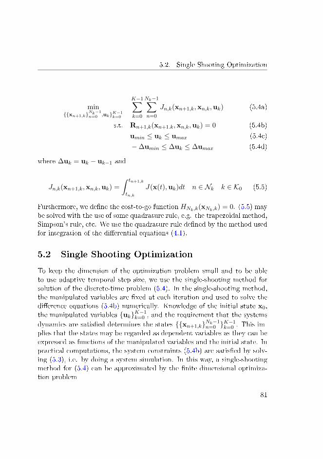
5.2. Single Shooting Optimization
minxn+1,k
Nk−1n=0 ,ukK−1
k=0
K−1∑
k=0
Nk−1∑
n=0
Jn,k(xn+1,k,xn,k,uk) (5.4a)
s.t. Rn+1,k(xn+1.k,xn,k,uk) = 0 (5.4b)
umin ≤ uk ≤ umax (5.4c)
−∆umin ≤ ∆uk ≤ ∆umax (5.4d)
where ∆uk = uk − uk−1 and
Jn,k(xn+1,k,xn,k,uk) =
∫ tn+1,k
tn,k
J(x(t),uk)dt n ∈ Nk k ∈ K0 (5.5)
Furthermore, we dene the cost-to-go function HNk,k(xNk,k) = 0. (5.5) maybe solved with the use of some quadrature rule, e.g. the trapezoidal method,Simpson's rule, etc. We use the quadrature rule dened by the method usedfor integration of the dierential equations (4.1).
5.2 Single Shooting Optimization
To keep the dimension of the optimization problem small and to be ableto use adaptive temporal step size, we use the single-shooting method forsolution of the discrete-time problem (5.4). In the single-shooting method,the manipulated variables are xed at each iteration and used to solve thedierence equations (5.4b) numerically. Knowledge of the initial state x0,the manipulated variables ukK−1
k=0 , and the requirement that the systems
dynamics are satised determines the states xn+1,kNk−1n=0 K−1
k=0 . This im-plies that the states may be regarded as dependent variables as they can beexpressed as functions of the manipulated variables and the initial state. Inpractical computations, the system constraints (5.4b) are satised by solv-ing (5.3), i.e. by doing a system simulation. In this way, a single-shootingmethod for (5.4) can be approximated by the nite dimensional optimiza-tion problem
81

5. Production Optimization
minukK−1
k=0
ψ(ukK−1k=0 ,x0) (5.6a)
s.t. umin ≤ uk ≤ umax (5.6b)
−∆umin ≤ ∆uk ≤ ∆umax (5.6c)
in which
ψ(ukK−1k=0 ,x0) =
K−1∑
k=0
Nk−1∑
n=0
Jn,k(xn+1,k,xn,k,uk) :
Rn+1,k(xn+1,k,xn,k,uk) = 0 n ∈ Nk k ∈ K0
(5.7)
is the objective function that only depends on the manipulated variablesand the xed initial state.
5.3 Gradient Computation by the Adjoint
Method
In solving the reduced system (5.6), we must compute the gradient ∇ukψ.The system states in dynamic optimization problems are dependent on thecontrol variables, in the sense that any past change of the control variableshas an inuence on all subsequent system states. Consequently, the gradientinformation of (5.7) is not directly accessible. The necessary information forcomputing∇ukψ is obtained during the simulation step at each optimizationiteration in the single-shooting approach. The adjoint method uses thisinformation eciently to compute the gradients.Assume that the manipulated variables ukK−1
k=0 satises the input con-straints (5.4c) and (5.4d). Thus, we may dene the Lagrangian of (5.4) asfollows
82
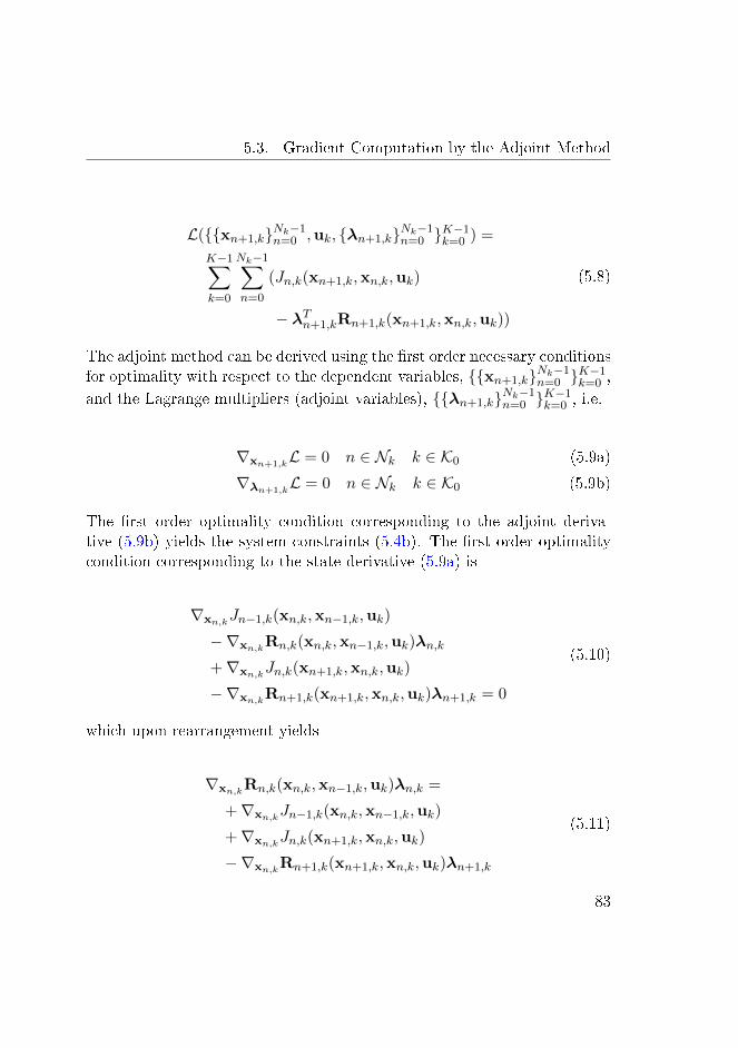
5.3. Gradient Computation by the Adjoint Method
L(xn+1,kNk−1n=0 ,uk, λn+1,kNk−1
n=0 K−1k=0 ) =
K−1∑
k=0
Nk−1∑
n=0
(Jn,k(xn+1,k,xn,k,uk)
− λTn+1,kRn+1,k(xn+1,k,xn,k,uk))
(5.8)
The adjoint method can be derived using the rst order necessary conditionsfor optimality with respect to the dependent variables, xn+1,kNk−1
n=0 K−1k=0 ,
and the Lagrange multipliers (adjoint variables), λn+1,kNk−1n=0 K−1
k=0 , i.e.
∇xn+1,kL = 0 n ∈ Nk k ∈ K0 (5.9a)
∇λn+1,kL = 0 n ∈ Nk k ∈ K0 (5.9b)
The rst order optimality condition corresponding to the adjoint deriva-tive (5.9b) yields the system constraints (5.4b). The rst order optimalitycondition corresponding to the state derivative (5.9a) is
∇xn,kJn−1,k(xn,k,xn−1,k,uk)
−∇xn,kRn,k(xn,k,xn−1,k,uk)λn,k
+∇xn,kJn,k(xn+1,k,xn,k,uk)
−∇xn,kRn+1,k(xn+1,k,xn,k,uk)λn+1,k = 0
(5.10)
which upon rearrangement yields
∇xn,kRn,k(xn,k,xn−1,k,uk)λn,k =
+∇xn,kJn−1,k(xn,k,xn−1,k,uk)
+∇xn,kJn,k(xn+1,k,xn,k,uk)
−∇xn,kRn+1,k(xn+1,k,xn,k,uk)λn+1,k
(5.11)
83

5. Production Optimization
from which we can compute the adjoint variables λnk in a backward recur-sion. The Lagrange multiplier at the nal time is λNK−1,K−1 = 0 since thecost-to-go function is zero. λNK−1,K−1 = 0 is used to initialize the back-ward march for computation of the adjoint variables λn,k, n ∈ Nk, k ∈ K0.Special attention must be given when computing λ0,k+1 at the transitionbetween uk and uk+1 for k ∈ 0, 1, . . . ,K − 2. At this point, the left-handside and the rst term on the right-hand side in (5.11) both belong to con-trol step uk, while the second and third term on the right-hand side belongto control step uk+1. When the state variables xn+1,kNk−1
n=0 K−1k=0 and the
adjoint variables λn+1,kNk−1n=0 K−1
k=0 satisfy (5.9), we have
ψ(ukK−1k=0 ,x0) =
L(xn+1,kNk−1
n=0 ,uk, λn+1,kNk−1n=0 K−1
k=0 ) :
Rn+1,k(xn+1,k,xn,k,uk) = 0 n ∈ Nk k ∈ K0
(5.12)
such that we can compute the sensitivity ∇ukψ as the sensitivity ∇ukL.Thus, considering the partial derivatives of (5.8) with respect to the manip-ulated variables ukK−1
k=0 , we may compute the gradients of the objectivefunction of the reduced system (5.6) as follows
∇ukψ(ukK−1k=0 ,x0) =
Nk−1∑
n=0
(∇ukJn,k(xn+1,k,xn,k,uk)
−∇ukRn+1,k(xn+1,k,xn,k,uk)λn+1,k)
k ∈ K0 (5.13)
The gradients ∇ukψ may be computed using (5.13) in combination withsolution of the adjoint equations (5.11) marching backwards. In Algorithm5.3.1 we show how to compute the gradients ∇ukψ, k ∈ K, using adjointsin a single shooting framework.
84
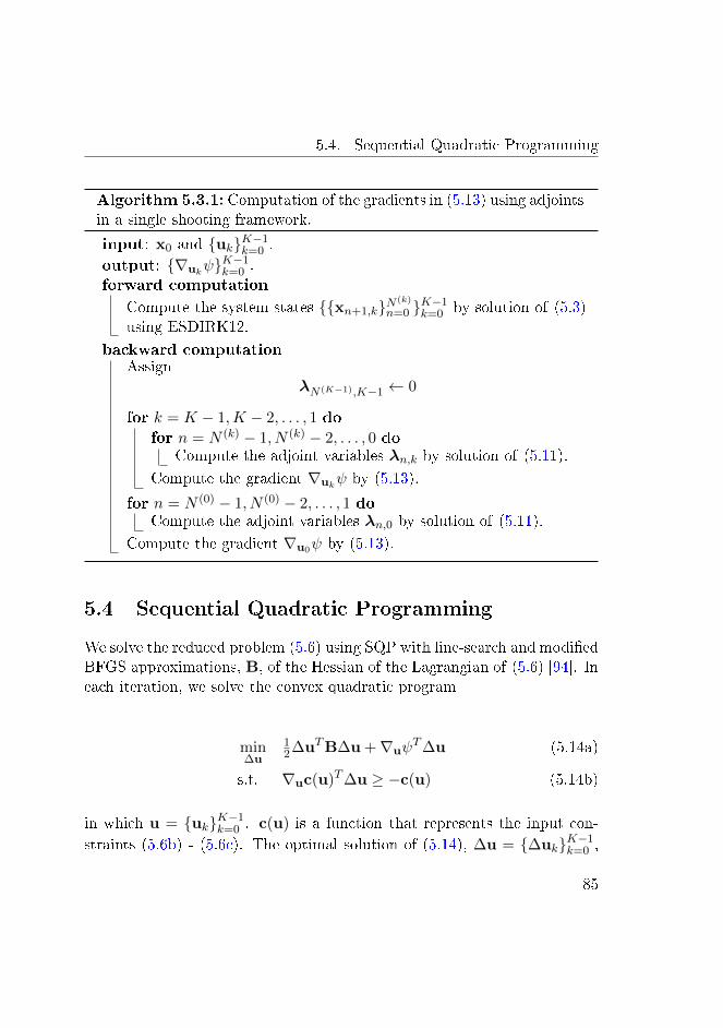
5.4. Sequential Quadratic Programming
Algorithm 5.3.1: Computation of the gradients in (5.13) using adjointsin a single shooting framework.
input: x0 and ukK−1k=0 .
output: ∇ukψK−1k=0 .
forward computation
Compute the system states xn+1,kN(k)
n=0 K−1k=0 by solution of (5.3)
using ESDIRK12.
backward computationAssign
λN(K−1),K−1 ← 0
for k = K − 1,K − 2, . . . , 1 do
for n = N (k) − 1, N (k) − 2, . . . , 0 doCompute the adjoint variables λn,k by solution of (5.11).
Compute the gradient ∇ukψ by (5.13).
for n = N (0) − 1, N (0) − 2, . . . , 1 doCompute the adjoint variables λn,0 by solution of (5.11).
Compute the gradient ∇u0ψ by (5.13).
5.4 Sequential Quadratic Programming
We solve the reduced problem (5.6) using SQP with line-search and modiedBFGS approximations, B, of the Hessian of the Lagrangian of (5.6) [94]. Ineach iteration, we solve the convex quadratic program
min∆u
12∆uTB∆u +∇uψ
T∆u (5.14a)
s.t. ∇uc(u)T∆u ≥ −c(u) (5.14b)
in which u = ukK−1k=0 . c(u) is a function that represents the input con-
straints (5.6b) - (5.6c). The optimal solution of (5.14), ∆u = ∆ukK−1k=0 ,
85

5. Production Optimization
Algorithm 5.4.1: Solution of the reduced problem (5.6) in an SQPframework using line-search and modied BFGS approximations.
input: x0 and an initial control strategy u.output: Optimal solution of u.while not optimal do
Compute ∆u by solving (5.14).Compute the line-search parameter α using Powell's exact penaltyfunction and update the manipulated variables u by (5.15).Compute the gradients ∇ukψK−1
k=0 cf. Algorithm 5.3.1.Update the Hessian in (5.14) using modied BFGS approximations.
combined with a line-search method based on Powell's exact penalty func-tion [95] are used to determine the next iterate
u(i+1) = u(i) + α(i)∆u(i) (5.15)
α(i) is the line-search parameter. Algorithm 5.4.1 outlines how we solve thereduced problem (5.6) in an SQP framework using line-search and modiedBFGS approximations.
5.5 Water Flooding Production Optimization
The objective of oil reservoir management is to maximize the economicvalue of the oil reservoir. Essentially, we want to produce as much oil aspossible while keeping the operational cost at a minimum. We do thisby maximizing the net present value (NPV). Consequently, the stage costJ(t) = J(t, x(t), u(t)) in (5.1) becomes
86

5.5. Water Flooding Production Optimization
J(t) = −e−dt ∑
j∈N pro
(rproo
ρoqproo,j (t)− rprow
ρwqprow,j(t)
)
−∑
j∈N injrinjw qinjj (t)
(5.16)
The factor e−dt accounts for the time value of capital. The terms contribut-ing to J(t) are the value of the produced oil, the cost of separating waterfrom the produced oil, and the cost of water injection. rproo is the oil price,rprow is the cost of water separation, and rinjw is the water injection cost.qproo,j (t) is the oil production and qprow,j(t) is the water production at produc-
tion wells, j ∈ N pro, at time t. qinjj (t) is the rate of injected water at the
injection wells, j ∈ N inj , at time t. The term d denotes the continuousdiscount rate (cost of capital per unit time).For water ooding using multiple injectors and producers, the well rates andpressures are adjusted by the optimal control problem (5.1) such that theNPV is maximized [1, 26]. The inequality constraints in (5.1) are boundconstraints (5.1c) and rate-of-change constraints (5.1d). The bound con-straints correspond to limitations on the water injection for each injectionwell and limitations on the BHP for each production well. The lower boundson the water injection rates are zero, while the upper bound is computedsuch that no more than a predened number of pore volumes (PVs) of waterare allowed to be injected over the time horizon considered, [t0, tf ]. Thatis, PVmax is the maximum amount of water that may be injected into thereservoir during the planned production period T = [t0, tf ]. These boundconstraints implies that we will implicitly satisfy
0 ≤N inj∑
j=1
K−1∑
k=0
Nk−1∑
n=0
∫ tn+1,k
tn,k
qinjj (t)dt ≤ PVmax (5.17)
The reservoir uids are trapped inside the pores of a porous medium. ThePV of a reservoir is dened by the fraction (the porosity) of the porous
87
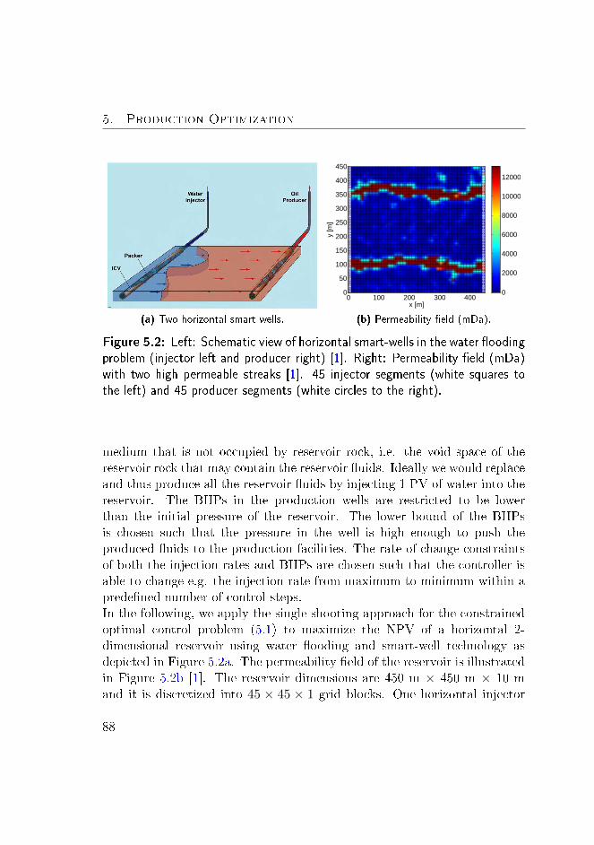
5. Production Optimization
(a) Two horizontal smart-wells.
x [m]
y [m
]
0 100 200 300 4000
50
100
150
200
250
300
350
400
450
0
2000
4000
6000
8000
10000
12000
(b) Permeability eld (mDa).
Figure 5.2: Left: Schematic view of horizontal smart-wells in the water oodingproblem (injector left and producer right) [1]. Right: Permeability eld (mDa)with two high permeable streaks [1]. 45 injector segments (white squares tothe left) and 45 producer segments (white circles to the right).
medium that is not occupied by reservoir rock, i.e. the void space of thereservoir rock that may contain the reservoir uids. Ideally we would replaceand thus produce all the reservoir uids by injecting 1 PV of water into thereservoir. The BHPs in the production wells are restricted to be lowerthan the initial pressure of the reservoir. The lower bound of the BHPsis chosen such that the pressure in the well is high enough to push theproduced uids to the production facilities. The rate-of-change constraintsof both the injection rates and BHPs are chosen such that the controller isable to change e.g. the injection rate from maximum to minimum within apredened number of control steps.In the following, we apply the single shooting approach for the constrainedoptimal control problem (5.1) to maximize the NPV of a horizontal 2-dimensional reservoir using water ooding and smart-well technology asdepicted in Figure 5.2a. The permeability eld of the reservoir is illustratedin Figure 5.2b [1]. The reservoir dimensions are 450 m × 450 m × 10 mand it is discretized into 45 × 45 × 1 grid blocks. One horizontal injector
88

5.5. Water Flooding Production Optimization
Symbol Description Value Unit
φ Porosity 0.2 -
Swc Critical water saturation 0.20 -Sor Residual oil saturation 0.15 -krw Water end point relative permeability 0.6 -kro Oil end point relative permeability 0.8 -nw Corey exponent, water 1.5 -no Corey exponent, oil 2.0 -
ρw Water density (at 1 atm) 1000 kg·m−3
ρo Oil density (at 1 atm) 800 kg·m−3
cw Water compressibility 10−5 atm−1
co Oil compressibility 10−5 atm−1
µw Water viscosity 1.0 cPµo Oil viscosity 1.0 cP
Sinit Initial water saturation 0.3 -Pinit Initial reservoir pressure 200 atm
Table 5.1: Reservoir properties.
Symbol Description Value Unit
rproo Oil price 283,0 $/m3
rprow Cost of water separation 31,5 $/m3
rinjw Cost of water injection 5,0 $/m3
d Discount rate 0 -
Table 5.2: Economic data [15, 26, 36].
divided into 45 individually controllable segments is positioned on the left-hand side of the reservoir (white squares, rst segment at (x, y) = (5, 5) m,last segment at (x, y) = (5, 445) m), and one horizontal producer dividedinto 45 individually controllable segments is positioned on the right-handside of the reservoir (white circles, rst segment at (x, y) = (445, 5) m,last segment at (x, y) = (445, 445) m). In this setup we mimic horizontal
89

5. Production Optimization
Symbol Description Value Unit
qinjmin Min. water injection rate per injector 0 m3·d−1
qinjmax Max. water injection rate per injector 50 m3·d−1
P bhmin Min. BHP in the producers 150 atmP bhmax Max. BHP in the producers 200 atm
∆qinjmin Min. rate of change of the water injection -3.85 m3·d−1
∆qinjmax Max. rate of change of the water injection 3.85 m3·d−1
∆P bhmin Min. rate of change of the BHP -3.85 atm∆P bhmax Max. rate of change of the BHP 3.85 atm
PVmax Max. amount of water allowed for injection 4Vp m3
T Planned production period 728 d
Table 5.3: Controller settings.
wells by composing multiple vertical wells. Each vertical well is completedin adjacent grid blocks, see Section 2.5, such that a vertical well mimics ahorizontal well segment. Table 5.1 lists the geological properties and theuid properties of the reservoir. The economical data are listed in Table5.2 [15, 26]. The discount rate is zero, d = 0 [36]. Table 5.3 provides theconstraints of the injection rates and the BHPs as well as the maximumallowed number of PVs to be injected during the production period.We apply two dierent production strategies. In the rst approach, weinject 2.00 PV over a period of 728 days (2 years) using xed injectionrates and BHPs. Throughout the 2-year production period, all injectorsegments are assigned the same constant injection rate, and all producersegments are assigned the same constant BHP. In the second approach, weapply optimized well rates and BHPs to the injectors and the producers,respectively. Each well segment is adjusted individually by the optimizerevery 28 days. As shown in Figure 5.3a, this strategy leads to an optimalproduction period of 374 days (1 year and 10 days) with an injection of only1.00 PV of water in total. Figure 5.3b illustrates injected PVs as function oftime. Figure 5.4a and 5.4b depicts the recovery factor (produced oil relatedto the initial mass of oil in the reservoir) and the water cut (produced
90
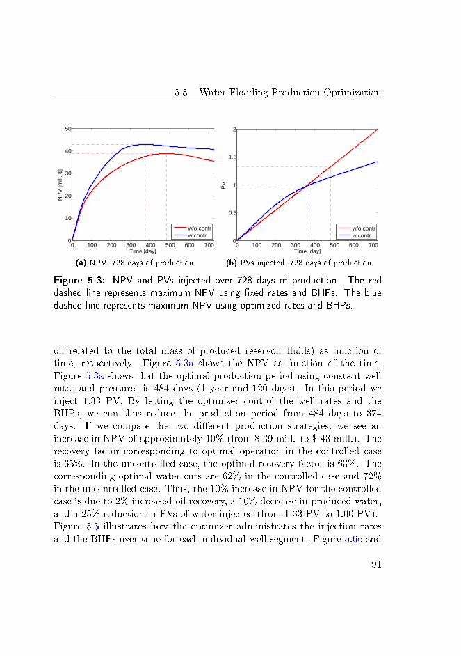
5.5. Water Flooding Production Optimization
0 100 200 300 400 500 600 7000
10
20
30
40
50
Time [day]
NP
V [m
ill. $
]
w/o contrw contr
(a) NPV, 728 days of production.
0 100 200 300 400 500 600 7000
0.5
1
1.5
2
Time [day]
PV
w/o contrw contr
(b) PVs injected, 728 days of production.
Figure 5.3: NPV and PVs injected over 728 days of production. The reddashed line represents maximum NPV using xed rates and BHPs. The bluedashed line represents maximum NPV using optimized rates and BHPs.
oil related to the total mass of produced reservoir uids) as function oftime, respectively. Figure 5.3a shows the NPV as function of the time.Figure 5.3a shows that the optimal production period using constant wellrates and pressures is 484 days (1 year and 120 days). In this period weinject 1.33 PV. By letting the optimizer control the well rates and theBHPs, we can thus reduce the production period from 484 days to 374days. If we compare the two dierent production strategies, we see anincrease in NPV of approximately 10% (from $ 39 mill. to $ 43 mill.). Therecovery factor corresponding to optimal operation in the controlled caseis 65%. In the uncontrolled case, the optimal recovery factor is 63%. Thecorresponding optimal water cuts are 62% in the controlled case and 72%in the uncontrolled case. Thus, the 10% increase in NPV for the controlledcase is due to 2% increased oil recovery, a 10% decrease in produced water,and a 25% reduction in PVs of water injected (from 1.33 PV to 1.00 PV).Figure 5.5 illustrates how the optimizer administrates the injection ratesand the BHPs over time for each individual well segment. Figure 5.6c and
91
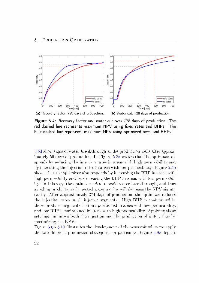
5. Production Optimization
0 100 200 300 400 500 600 7000
0.1
0.2
0.3
0.4
0.5
0.6
0.7
0.8
Time [day]
Rec
over
y
w/o contrw contr
(a) Recovery factor, 728 days of production.
0 100 200 300 400 500 600 7000
0.1
0.2
0.3
0.4
0.5
0.6
0.7
0.8
Time [day]W
ater
cut
w/o contrw contr
(b) Water cut, 728 days of production.
Figure 5.4: Recovery factor and water cut over 728 days of production. Thered dashed line represents maximum NPV using xed rates and BHPs. Theblue dashed line represents maximum NPV using optimized rates and BHPs.
5.6d show signs of water-breakthrough at the production wells after approx-imately 50 days of production. In Figure 5.5a we see that the optimizer re-sponds by reducing the injection rates in areas with high permeability andby increasing the injection rates in areas with low permeability. Figure 5.5bshows that the optimizer also responds by increasing the BHP in areas withhigh permeability and by decreasing the BHP in areas with low permeabil-ity. In this way, the optimizer tries to avoid water breakthrough, and thusavoiding production of injected water as this will decrease the NPV signi-cantly. After approximately 374 days of production, the optimizer reducesthe injection rates in all injector segments. High BHP is maintained inthose producer segments that are positioned in areas with low permeability,and low BHP is maintained in areas with high permeability. Applying thesesettings minimizes both the injection and the production of water, therebymaximizing the NPV.Figure 5.6 - 5.10 illustrates the development of the reservoir when we applythe two dierent production strategies. In particular, Figure 5.9e depicts
92
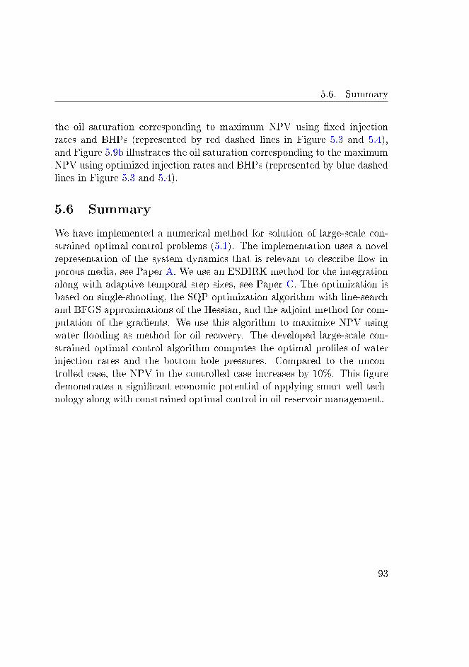
5.6. Summary
the oil saturation corresponding to maximum NPV using xed injectionrates and BHPs (represented by red dashed lines in Figure 5.3 and 5.4),and Figure 5.9b illustrates the oil saturation corresponding to the maximumNPV using optimized injection rates and BHPs (represented by blue dashedlines in Figure 5.3 and 5.4).
5.6 Summary
We have implemented a numerical method for solution of large-scale con-strained optimal control problems (5.1). The implementation uses a novelrepresentation of the system dynamics that is relevant to describe ow inporous media, see Paper A. We use an ESDIRK method for the integrationalong with adaptive temporal step sizes, see Paper C. The optimization isbased on single-shooting, the SQP optimization algorithm with line-searchand BFGS approximations of the Hessian, and the adjoint method for com-putation of the gradients. We use this algorithm to maximize NPV usingwater ooding as method for oil recovery. The developed large-scale con-strained optimal control algorithm computes the optimal proles of waterinjection rates and the bottom hole pressures. Compared to the uncon-trolled case, the NPV in the controlled case increases by 10%. This guredemonstrates a signicant economic potential of applying smart well tech-nology along with constrained optimal control in oil reservoir management.
93

5. Production Optimization
Time [day]
y [m
]
0 200 400 6000
50
100
150
200
250
300
350
400
450
12
14
16
18
20
22
24
26
28
30
32
(a) Individual injection rates (m3/day) of 45 injectors.
Time [day]
y [m
]
0 200 400 6000
50
100
150
200
250
300
350
400
450
150
155
160
165
170
175
(b) Individual BHPs (atm) of 45 producers.
Figure 5.5: Injection rates and BHPs over 728 days of production, updatedeach 28 days. The injectors and producers are depicted in Figure 5.2b.
94

5.6. Summary
x [m]
y [m
]
0 100 200 300 4000
50
100
150
200
250
300
350
400
450
0.15
0.2
0.25
0.3
0.35
0.4
0.45
0.5
0.55
0.6
0.65
(a) 0.07 PV, 25 days, xed.
x [m]
y [m
]
0 100 200 300 4000
50
100
150
200
250
300
350
400
450
0.15
0.2
0.25
0.3
0.35
0.4
0.45
0.5
0.55
0.6
0.65
(b) 0.07 PV, 25 days, optimized.
x [m]
y [m
]
0 100 200 300 4000
50
100
150
200
250
300
350
400
450
0.15
0.2
0.25
0.3
0.35
0.4
0.45
0.5
0.55
0.6
0.65
(c) 0.14 PV, 50 days, xed.
x [m]
y [m
]
0 100 200 300 4000
50
100
150
200
250
300
350
400
450
0.15
0.2
0.25
0.3
0.35
0.4
0.45
0.5
0.55
0.6
0.65
(d) 0.14 PV, 50 days, optimized.
x [m]
y [m
]
0 100 200 300 4000
50
100
150
200
250
300
350
400
450
0.15
0.2
0.25
0.3
0.35
0.4
0.45
0.5
0.55
0.6
0.65
(e) 0.21 PV, 75 days, xed.
x [m]
y [m
]
0 100 200 300 4000
50
100
150
200
250
300
350
400
450
0.15
0.2
0.25
0.3
0.35
0.4
0.45
0.5
0.55
0.6
0.65
(f) 0.24 PV, 75 days, optimized.
Figure 5.6: Oil saturations after 25, 50 and 75 days of production. Leftcolumn: with the use of xed injection rates and BHPs. Right column: withthe use of optimized injection rates and BHPs.
95

5. Production Optimization
x [m]
y [m
]
0 100 200 300 4000
50
100
150
200
250
300
350
400
450
0.15
0.2
0.25
0.3
0.35
0.4
0.45
0.5
0.55
0.6
0.65
(a) 0.28 PV, 100 days, xed.
x [m]
y [m
]
0 100 200 300 4000
50
100
150
200
250
300
350
400
450
0.15
0.2
0.25
0.3
0.35
0.4
0.45
0.5
0.55
0.6
0.65
(b) 0.33 PV, 100 days, optimized.
x [m]
y [m
]
0 100 200 300 4000
50
100
150
200
250
300
350
400
450
0.15
0.2
0.25
0.3
0.35
0.4
0.45
0.5
0.55
0.6
0.65
(c) 0.41 PV, 125 days, xed.
x [m]
y [m
]
0 100 200 300 4000
50
100
150
200
250
300
350
400
450
0.15
0.2
0.25
0.3
0.35
0.4
0.45
0.5
0.55
0.6
0.65
(d) 0.50 PV, 125 days, optimized.
x [m]
y [m
]
0 100 200 300 4000
50
100
150
200
250
300
350
400
450
0.15
0.2
0.25
0.3
0.35
0.4
0.45
0.5
0.55
0.6
0.65
(e) 0.56 PV, 150 days, xed.
x [m]
y [m
]
0 100 200 300 4000
50
100
150
200
250
300
350
400
450
0.15
0.2
0.25
0.3
0.35
0.4
0.45
0.5
0.55
0.6
0.65
(f) 0.64 PV, 150 days, optimized.
Figure 5.7: Oil saturations after 100, 150 and 200 days of production. Leftcolumn: with the use of xed injection rates and BHPs. Right column: withthe use of optimized injection rates and BHPs.
96
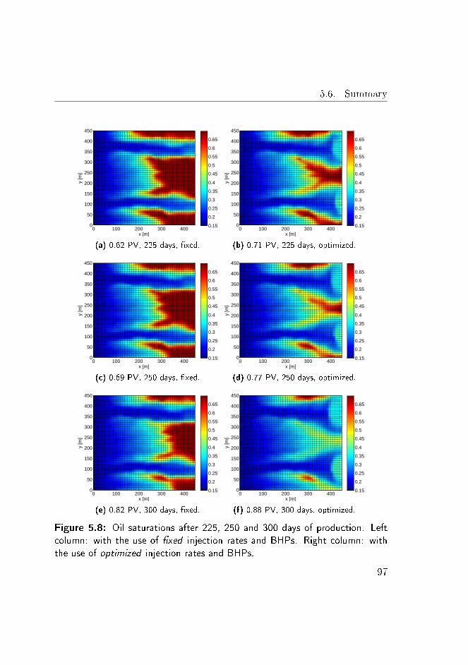
5.6. Summary
x [m]
y [m
]
0 100 200 300 4000
50
100
150
200
250
300
350
400
450
0.15
0.2
0.25
0.3
0.35
0.4
0.45
0.5
0.55
0.6
0.65
(a) 0.62 PV, 225 days, xed.
x [m]
y [m
]
0 100 200 300 4000
50
100
150
200
250
300
350
400
450
0.15
0.2
0.25
0.3
0.35
0.4
0.45
0.5
0.55
0.6
0.65
(b) 0.71 PV, 225 days, optimized.
x [m]
y [m
]
0 100 200 300 4000
50
100
150
200
250
300
350
400
450
0.15
0.2
0.25
0.3
0.35
0.4
0.45
0.5
0.55
0.6
0.65
(c) 0.69 PV, 250 days, xed.
x [m]
y [m
]
0 100 200 300 4000
50
100
150
200
250
300
350
400
450
0.15
0.2
0.25
0.3
0.35
0.4
0.45
0.5
0.55
0.6
0.65
(d) 0.77 PV, 250 days, optimized.
x [m]
y [m
]
0 100 200 300 4000
50
100
150
200
250
300
350
400
450
0.15
0.2
0.25
0.3
0.35
0.4
0.45
0.5
0.55
0.6
0.65
(e) 0.82 PV, 300 days, xed.
x [m]
y [m
]
0 100 200 300 4000
50
100
150
200
250
300
350
400
450
0.15
0.2
0.25
0.3
0.35
0.4
0.45
0.5
0.55
0.6
0.65
(f) 0.88 PV, 300 days, optimized.
Figure 5.8: Oil saturations after 225, 250 and 300 days of production. Leftcolumn: with the use of xed injection rates and BHPs. Right column: withthe use of optimized injection rates and BHPs.
97
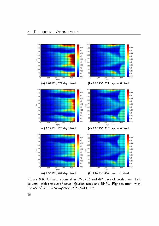
5. Production Optimization
x [m]
y [m
]
0 100 200 300 4000
50
100
150
200
250
300
350
400
450
0.15
0.2
0.25
0.3
0.35
0.4
0.45
0.5
0.55
0.6
0.65
(a) 1.04 PV, 374 days, xed.
x [m]
y [m
]
0 100 200 300 4000
50
100
150
200
250
300
350
400
450
0.15
0.2
0.25
0.3
0.35
0.4
0.45
0.5
0.55
0.6
0.65
(b) 1.00 PV, 374 days, optimized.
x [m]
y [m
]
0 100 200 300 4000
50
100
150
200
250
300
350
400
450
0.15
0.2
0.25
0.3
0.35
0.4
0.45
0.5
0.55
0.6
0.65
(c) 1.17 PV, 425 days, xed.
x [m]
y [m
]
0 100 200 300 4000
50
100
150
200
250
300
350
400
450
0.15
0.2
0.25
0.3
0.35
0.4
0.45
0.5
0.55
0.6
0.65
(d) 1.07 PV, 425 days, optimized.
x [m]
y [m
]
0 100 200 300 4000
50
100
150
200
250
300
350
400
450
0.15
0.2
0.25
0.3
0.35
0.4
0.45
0.5
0.55
0.6
0.65
(e) 1.33 PV, 484 days, xed.
x [m]
y [m
]
0 100 200 300 4000
50
100
150
200
250
300
350
400
450
0.15
0.2
0.25
0.3
0.35
0.4
0.45
0.5
0.55
0.6
0.65
(f) 1.14 PV, 484 days, optimized.
Figure 5.9: Oil saturations after 374, 425 and 484 days of production. Leftcolumn: with the use of xed injection rates and BHPs. Right column: withthe use of optimized injection rates and BHPs.
98

5.6. Summary
x [m]
y [m
]
0 100 200 300 4000
50
100
150
200
250
300
350
400
450
0.15
0.2
0.25
0.3
0.35
0.4
0.45
0.5
0.55
0.6
0.65
(a) 1.44 PV, 525 days, xed.
x [m]
y [m
]
0 100 200 300 4000
50
100
150
200
250
300
350
400
450
0.15
0.2
0.25
0.3
0.35
0.4
0.45
0.5
0.55
0.6
0.65
(b) 1.19 PV, 525 days, optimized.
x [m]
y [m
]
0 100 200 300 4000
50
100
150
200
250
300
350
400
450
0.15
0.2
0.25
0.3
0.35
0.4
0.45
0.5
0.55
0.6
0.65
(c) 1.72 PV, 625 days, xed.
x [m]
y [m
]
0 100 200 300 4000
50
100
150
200
250
300
350
400
450
0.15
0.2
0.25
0.3
0.35
0.4
0.45
0.5
0.55
0.6
0.65
(d) 1.30 PV, 625 days, optimized.
x [m]
y [m
]
0 100 200 300 4000
50
100
150
200
250
300
350
400
450
0.15
0.2
0.25
0.3
0.35
0.4
0.45
0.5
0.55
0.6
0.65
(e) 2.00 PV, 728 days, xed.
x [m]
y [m
]
0 100 200 300 4000
50
100
150
200
250
300
350
400
450
0.15
0.2
0.25
0.3
0.35
0.4
0.45
0.5
0.55
0.6
0.65
(f) 1.42 PV, 728 days, optimized.
Figure 5.10: Oil saturations after 525, 625 and 728 days of production. Leftcolumn: with the use of xed injection rates and BHPs. Right column: withthe use of optimized injection rates and BHPs.
99

CHAPTER 6Conclusion
The primary focus of the work in this thesis has been the application of massconserving high order explicit singly diagonal implicit Runge-Kutta (ES-DIRK) methods with embedded error estimators for step size control andthe adjoint approach for gradient computation in a single-shooting frame-work with emphasis on optimal control of the water ooding process foroil recovery. The overall achievements of the work are summarized in thischapter.
• We have implemented the immiscible two-phase ow problem for sim-ulation of combined ow of water and oil in isothermal reservoirs withheterogenous isotropic permeability eld. The well models are basedon the Peaceman well index for vertical wells in non-square Cartesiangrids. Injection wells are operated at variable injection rates, whereasproduction wells are operated at variable bottom hole pressure (BHP).
• The uid ow in the reservoir model is governed by a system of partialdierential equations (PDEs). We use the method of lines for solutionof the model. We have discretized the model spatially using the nite
101
6. Conclusion
volume method (FVM), and we have applied the two point ux ap-proximation (TPFA) and the single-point upstream (SPU) scheme forcomputing the interface uxes of the water and oil phases. We solvethe spatially discretized model using a fully implicit mass conservinghigh order method for numerical integration.
• We have proposed a new mass conserving formulation of the dier-ential equation system that arise as a consequence of the spatial dis-cretization of the two-phase ow model. The two-phase ow modelis developed under the assumption of mass conservation. In general,process system models are based on conservation of mass, energy andmomentum, and they can be directly represented in the form of theproposed dierential equation system. Upon discretization in time,the proposed equation system ensures the preservation of such prop-erties.
• We have presented the family of Runge-Kutta integration methods,and we have developed new mass conserving ESDIRK methods withembedded error estimators for adaptive step size control. In situationswhere solutions with high accuracy is required, we have demonstratedthat high-order ESDIRK methods can provide a solution of the wa-ter ooding problem more eciently than the traditional low-ordermethods, often referred to in the petroleum literature as: the implicitpressure explicit saturation (IMPES) method, the sequential implicitmethod (SIM), and the fully implicit method (FIM).
• Current reservoir simulation tools use step size control, which is basedon safeguarded heuristics. These can neither deliver solutions withpredetermined accuracy or guarantee the convergence in the modiedNewton-Raphson (NR) iterations. We have established predictive stepsize control based on error estimates, which can be calculated from theembedded ESDIRK methods. The adaptive step size control monitorsboth the integration error of the solution and the convergence of theiterative solver. We have added some modications to both error andconvergence monitoring in order to achieve a smoother control of the
102
integration error. In this way we minimize the computational cost persimulation of the two-phase ow problem.
• We have used nonlinear model predictive control (NMPC) to maxi-mize the net present value (NPV) of an oil reservoir by manipulat-ing injection rates and BHPs of injection wells and production wells,respectively. We have implemented a single-shooting method for so-lution of large-scale constrained optimization problems. The forwardintegration is done using ESDIRK methods along with adaptive tem-poral step sizes. The optimization is based on quasi-Newton sequentialquadratic programming (SQP) with line-search and BFGS approxi-mations of the Hessian, and the adjoint method for ecient computa-tion of the gradients. We have demonstrated that the application ofNMPC for optimal control of smart-wells has the potential to increasethe economic value of an oil reservoir.
103


Bibliography
[1] D. Brouwer and J.-D. Jansen, Dynamic optimization of wateroodingwith smart wells using optimal control theory, SPE Journal, vol. 9,no. 4, pp. 391402, 2004.
[2] M. Konopczynski, Design and modelling of intelligent well downholevalves for adjustable ow control of smart wells, presented at the SPEATW Modeling and Optimization of Smart Wells, 2005.
[3] D. Brouwer, G. Nævdal, J. Jansen, E. Vefring, and C. vanKruijsdijk, Improved reservoir management through optimal controland continuous model updating, in SPE Annual Technical Conferenceand Exhibition, Houston, Texas, 2004.
[4] M. Handels, M. Zandvliet, R. Brouwer, and J. D. Jansen, Adjoint-based well-placement optimization under production constraints, inSPE Reservoir Simulation Symposium. Houston, Texas, U.S.A.:Society of Petroleum Engineers, 2007.
[5] M. Zandvliet, Model-based lifecycle optimization of well locationsand production settings in petroleum reservoirs, Ph.D. dissertation,2008.
[6] P. Sarma and W. H. Chen, Applications of optimal controltheory for ecient production optimisation of realistic reservoirs,in International Petroleum Technology Conference. Kuala Lumpur,Malaysia: International Petroleum Technology Conference, 2008.
105
Bibliography
[7] W. Chen, G. Gavalas, J. Seinfeld, and M. Wasserman, A newalgorithm for automatic history matching, no. 12, 1974.
[8] G. CHAVENT, M. DUPUY, and P. LEMONNIER, History matchingby use of optimal theory, no. 02, 1975.
[9] W. F. Ramirez, Application of Optimal Control Theory to EnhancedOil Recovery, ser. Developments in Petroleum Science. New York,US: Elsevier Science Inc., 1987, vol. 21.
[10] D. R. Brouwer, Dynamic water ood optimization with smart wellsusing optimal control theory, Ph.D. dissertation, Delft, NL, 2004.
[11] B. Sudaryanto and Y. C. Yortsos, Optimization of uid frontdynamics in porous media using rate control. i. equal mobility uids,Physics of Fluids, vol. 12, no. 7, pp. 16561670, 2000.
[12] B. Sudaryanto and Y. C. Yortsos, Optimization of displacements inporous media using rate control, in SPE Annual Technical Conferenceand Exhibition. New Orleans, Louisiana: Copyright 2001, Society ofPetroleum Engineers Inc., 2001.
[13] P. Sarma, K. Aziz, and L. Durlofsky, Implementation of adjoint solu-tion for optimal control of smart wells, in SPE Reservoir SimulationSymposium. The Woodlands, Texas: 2005,. Society of Petroleum En-gineers Inc., 2005.
[14] P. de Montleau, A. Cominelli, K. Neylon, D. Rowan, I. Pallister,O. Tesaker, and I. Nygard, Production optimization under constraintsusing adjoint gradients, in Proceedings of ECMOR X. Amsterdam,NL: European Association of Geoscientists and Engineers, Sept. 2006.
[15] J. F. B. M. Kraaijevanger, P. J. Egberts, J. R. Valstar, and H. W. Bu-urman, Optimal waterood design using the adjoint method, in SPEReservoir Simulation Symposium. Houston, Texas, U.S.A.: Society ofPetroleum Engineers, 2007.
106
Bibliography
[16] G. van Essen, M. Zandvliet, P. V. den Hof, O. Bosgra, and J.-D.Jansen, Robust waterooding optimization of multiple geologicalscenarios, SPE Journal, no. 03, 2009.
[17] G. van Essen, J.-D. Jansen, R. Brouwer, S. G. Douma, M. Zandvliet,K. I. Rollett, and D. Harris, Optimization of smart wells in the st.joseph eld, SPE Reservoir Evaluation & Engineering, no. 08, 2010.
[18] P. Sarma, W. H. Chen, L. J. Durlofsky, and K. Aziz, Productionoptimization with adjoint models under nonlinear control-statepath inequality constraints, in Intelligent Energy Conference andExhibition. Amsterdam, The Netherlands: Society of PetroleumEngineers, 2006.
[19] E. Suwartadi, S. Krogstad, and B. Foss, On state constraints of adjointoptimization in oil reservoir waterooding, in SPE/EAGE ReservoirCharacterization and Simulation Conference. Abu Dhabi, UAE: So-ciety of Petroleum Engineers, 2009.
[20] E. Suwartadi, S. Krogstad, and B. Foss, A lagrangian-barrier functionfor adjoint state constraints optimization of oil reservoirs water ood-ing, in Decision and Control (CDC), 2010 49th IEEE Conference on,dec. 2010, pp. 3884 3889.
[21] E. Suwartadi, S. Krogstad, and B. Foss, Nonlinear output constraintshandling for production optimization of oil reservoirs, ComputationalGeosciences, pp. 119, 2011, 10.1007/s10596-011-9253-3.
[22] E. Suwartadi, S. Krogstad, and B. Foss, Second-order adjoint-basedcontrol for multiphase ow in subsurface oil reservoirs, in Decision andControl (CDC), 2010 49th IEEE Conference on, dec. 2010, pp. 18661871.
[23] G. Naevdal, T. Mannseth, and E. H. Vefring, Instrumented wells andnear-well reservoir monitoring through ensemble kalman lter, in Pro-ceedings of ECMOR VIII. Freiberg, DE: European Association ofGeoscientists and Engineers, Sept. 2002.
107
Bibliography
[24] G. Naevdal, D. Brouwer, and J.-D. Jansen, Waterooding usingclosed-loop control, pp. 3760, 2006-03-26.
[25] J.-D. Jansen, O. H. Bosgra, and P. M. Van den Hof, Model-based con-trol of multiphase ow in subsurface oil reservoirs, Journal of ProcessControl, vol. 18, no. 9, pp. 846855, Oct. 2008.
[26] J.-D. Jansen, R. Brouwer, and S. G. Douma, Closed loop reservoirmanagement, in SPE Reservoir Simulation Symposium. The Wood-lands, Texas: Society of Petroleum Engineers, 2009.
[27] P. Sarma, L. Durlofsky, K. Aziz, and W. Chen, Ecient real-timereservoir management using adjoint-based optimal control and modelupdating, Computational Geosciences, vol. 10, pp. 336, 2006,10.1007/s10596-005-9009-z.
[28] C. Chen, G. Li, and A. C. Reynolds, Robust constrained optimizationof short and long-term npv for closed-loop reservoir management, inSPE Reservoir Simulation Symposium. The Woodlands, Texas, USA:Society of Petroleum Engineers, 2011.
[29] L. Peters, R. Arts, G. Brouwer, C. Geel, S. Cullick, R. J. Lorentzen,Y. Chen, N. Dunlop, F. C. Vossepoel, R. Xu, P. Sarma, A. H.Alhuthali, and A. Reynolds, Results of the brugge benchmark studyfor ooding optimization and history matching, SPE ReservoirEvaluation & Engineering, no. 06, 2010.
[30] D. W. Peaceman, Fundamentals of Numerical Reservoir Simulation.Amsterdam, Holland: Developments in Petroleum Science, 1977, vol. 6.
[31] K. Aziz and A. Settari, Petroleum Reservoir Simulation, 1st ed. Lon-don: Applied Science Publishers Ltd, 1979.
[32] H. Tchelepi and K. Aziz, Advances in reservoir simulation, in InProceedings of the 8th International Forum on Reservoir Simulation,Stresa, Italy, 2005.
108
Bibliography
[33] M. G. Gerritsen and L. J. Durlofsky, Modeling uid ow in oilreservoirs, Annual Review of Fluid Mechanics, vol. 37, no. 1, pp.211238, 2005.
[34] Z. Chen, Reservoir Simulation : Mathematical Techniques in Oil Re-covery. Philadelphia: Society for Industrial and Applied Mathematics(SIAM), 2007.
[35] D. W. Peaceman, Interpretation of well-block pressures in numericalreservoir simulation with nonsquare grid blocks and anisotropic perme-ability, SPEJ, Society of Petroleum Engineers Journal, vol. 23, no. 3,pp. 531543, 1983.
[36] P. Sarma, W. H. Chen, L. J. Durlofsky, and K. Aziz, Production op-timization with adjoint models under nonlinear control-state path in-equality constraints, SPE Reservoir Evaluation & Engineering, vol. 11,no. 2, pp. 326339, 2008.
[37] J. D. Jansen, Adjoint-based optimization of multi-phase ow throughporous media - a review, Computers & Fluids, vol. 46, no. 1, pp.40 51, 2011, <ce:title>10th ICFD Conference Series on NumericalMethods for Fluid Dynamics (ICFD 2010)</ce:title>.
[38] A. T. Corey, The interrelation between gas and oil relative permeabil-ities, Producers Monthly, vol. 19, pp. 38 41, 1954.
[39] R. A. Berenblyum, A. A. Shapiro, E. H. Stenby, K. Jessen, and F. M.Orr Jr., Black oil streamline simulator with capillary eects, Proceed-ings - SPE Annual Technical Conference and Exhibition, pp. 133141,2003.
[40] H. P. G. Darcy, Les Fontaines Publiques de la Ville de Dijon, Dalmont,Paris, 1856.
[41] D. Peaceman, Interpretation of well-block pressures in numericalreservoir simulation (includes associated paper 6988), no. 06, 1978.
109
Bibliography
[42] J. H. Abou-Kassem and K. Aziz, Analytical well models for reservoirsimulation, no. 08, 1985.
[43] C. Palagi and K. Aziz, Modeling vertical and horizontal wells withvoronoi grid, SPE Reservoir Engineering, no. 02, 1994.
[44] J. A. Holmes, Modeling advanced wells in reservoir simulation, SPEJournal of Petroleum Technology, no. 11, 2001.
[45] C. Wolfsteiner, L. Durlofsky, and K. Aziz, Approximate model forproductivity of nonconventional wells in heterogeneous reservoirs,SPE Journal, no. 06, 2000.
[46] C. Wolfsteiner, L. J. Durlofsky, and K. Aziz, Calculation of well in-dex for nonconventional wells on arbitrary grids, Computational Geo-sciences, vol. 7, no. 1, pp. 6182, 2003.
[47] C. Guichard, J. Brac, R. Eymard, and R. Masson, Finite volumeschemes for multiphase ow simulation on near well grids, in Pro-ceedings of ECMOR XII. Oxford, UK: European Association of Geo-scientists and Engineers, Sept. 2010.
[48] I. Aavatsmark and R. Klausen, Well index in reservoir simulation forslanted and slightly curved wells in 3d grids, SPE Journal, no. 03,2003.
[49] R. J. LeVeque, Finite dierence methods for ordinary and partialdierential equations : Steady-State and Time-Dependent Problems.Philadelphia, US: Society for Industrial and Applied Mathematics(SIAM), 2007.
[50] I. Aavatsmark, Interpretation of a two-point ux stencil for skewparallelogram grids, Computational Geosciences, vol. 11, pp. 199206,2007, 10.1007/s10596-007-9042-1.
[51] M. G. Edwards and C. F. Rogers, Finite volume discretizationwith imposed ux continuity for the general tensor pressure
110

Bibliography
equation, Computational Geosciences, vol. 2, pp. 259290, 1998,10.1023/A:1011510505406.
[52] G. T. Eigestad and R. A. Klausen, On the convergence of themulti-point ux approximation o-method: Numerical experimentsfor discontinuous permeability, Numerical Methods for PartialDierential Equations, vol. 21, no. 6, pp. 10791098, 2005.
[53] Y. Chen, B. Mallison, and L. Durlofsky, Nonlinear two-point uxapproximation for modeling full-tensor eects in subsurface owsimulations, Computational Geosciences, vol. 12, pp. 317335, 2008,10.1007/s10596-007-9067-5.
[54] I. Aavatsmark, An introduction to multipoint ux approximations forquadrilateral grids, Computational Geosciences, vol. 6, pp. 405432,2002, 10.1023/A:1021291114475.
[55] Q.-Y. Chen, R. T. Miin, J. Wan, and Y. Yang, A new multipointux approximation for reservoir simulation, in SPE ReservoirSimulation Symposium, Houston, Texas, U.S.A., 2007.
[56] I. Aavatsmark, G. Eigestad, B.-O. Heimsund, B. Mallison,J. Nordbotten, and E. Øian, A new nite-volume approach to ecientdiscretization on challenging grids, SPE Journal, no. 09, 2010.
[57] E. Keilegavlen and I. Aavatsmark, Monotonicity for control vol-ume methods on unstructured grids, in Proceedings of ECMOR XI.Bergen, Norway: European Association of Geoscientists and Engineers,Sept. 2008.
[58] R. Yorgova and I. Aavatsmark, Modication of a reservoir grid toachieve monotonicity of the control volume method, in Proceedings ofECMOR XII. Oxford, UK: European Association of Geoscientists andEngineers, Sept. 2010.
111

Bibliography
[59] Z. Chen, G. Huan, and Y. Ma, Computational Methods for MultiphaseFlows in Porous Media, 2nd ed., ser. Computational science & engi-neering. Philadelphia: Society for Industrial and Applied Mathematics(SIAM), 2006.
[60] Y. Epshteyn and B. Riviere, Fully implicit discontinuous niteelement methods for two-phase ow, Applied Numerical Mathematics,vol. 57, no. 4, pp. 383 401, 2007.
[61] J. R. Natvig and K.-A. Lie, Fast computation of multiphase ow inporous media by implicit discontinuous galerkin schemes with opti-mal ordering of elements, Journal of Computational Physics, vol. 227,no. 24, pp. 10 10810 124, 2008.
[62] G. Pencheva, S. Thomas, and M. Wheeler, Mortar coupling of discon-tinuous galerkin and mixed nite element methods, in Proceedings ofECMOR XI. Bergen, Norway: European Association of Geoscientistsand Engineers, Sept. 2008.
[63] J. S. Hesthaven and T. Warburton, Nodal Discontinuous GalerkinMethods : Algorithms, Analysis and Applications. New York, USA:Springer Science+Business Media, LLC, 2008.
[64] J. D. Huppler, Waterood relative permeabilities in composite cores,J. Pet. Technol., vol. 21, pp. 539540, 1969.
[65] H. Versteeg and W. Malalasekera, An Introduction to ComputationalFluid Dynamics : The Finite Volume Method, 2nd ed. Harlow, Eng-land: Pearson Education Limited, 2007.
[66] R. Alexander, Design and implementation of dirk integrators for stisystems, Applied Numerical Mathematics, vol. 46, no. 1, pp. 1 17,2003.
[67] A. Kværnø, Singly diagonally implicit runge-kutta methods with anexplicit rst stage, BIT Numerical Mathematics, vol. 44, pp. 489 502, 2004.
112
Bibliography
[68] M. R. Kristensen, J. B. Jørgensen, P. G. Thomsen, and S. B. Jøgensen,An esdirk method with sensitivity analysis capabilities, Computers& Chemical Engineering, vol. 28, no. 12, pp. 2695 2707, 2004.
[69] J. B. Jørgensen, M. R. Kristensen, and P. G. Thomsen, A family of es-dirk integration methods, manuscript for SIAM Journal on ScienticComputing, 2008.
[70] J. Sheldon, B. Zondek, and W. C. Jr., One-dimensional,incompressible, noncapillary, two-phase uid ow in a porousmedium, 1959.
[71] H. Stone and A. G. Jr., Analysis of gas-cap or dissolved-gas drivereservoirs, no. 06, 1961.
[72] K. Coats, A note on impes and some impes-based simulation models,SPE Journal, vol. 5, no. 3, pp. 245251, 2000.
[73] A. Spillette, J. Hillestad, and H. Stone, A high-stability sequentialsolution approach to reservoir simulation, in Fall Meeting of theSociety of Petroleum Engineers of AIME, Las Vegas, Nevada, 1973.
[74] J. Watts, A compositional formulation of the pressure and saturationequations, SPE Reservoir Engineering, no. 05, 1986.
[75] J. Grabowski, P. Vinsome, R. C. Lin, G. Behie, and B. Rubin, Afully implicit general purpose nite-dierence thermal model for insitu combustion and steam, in SPE Annual Technical Conference andExhibition, Las Vegas, Nevada, 1979.
[76] K. H. Coats, In-situ combustion model, no. 12, 1980.
[77] R. Mehra, M. Hadjito, and J. K. Donnelly, An automatictime-step selector for reservoir models, in SPE Reservoir SimulationSymposium, New Orleans, Louisiana, 1982.
[78] P. Sammon and B. Rubin, Practical control of timestep selection inthermal simulation, SPE Reservoir Engineering, no. 03, 1986.
113
Bibliography
[79] C. A. Kennedy and M. H. Carpenter, Additive runge-kutta schemesfor convection-diusion-reaction equations, Applied Numerical Math-ematics, vol. 44, no. 1-2, pp. 139 181, 2003.
[80] K. Gustafsson, Control of error and convergence in ODE solvers,Ph.D. dissertation, Department of Automatic Control, Lund Univer-sity, Sweden, Mar. 1992.
[81] E. Hairer and G. Wanner, Solving Ordinary Dierential Equations II:Sti and Dierential-Algebraic Problems, 2nd ed. Springer, 1996.
[82] R. Alexander, The modied newton method in the solution of stiordinary dierential equations, Mathematics of Computation, vol. 57,no. 196, pp. 673701, 1991.
[83] N. Houbak, S. Nörsett, and P. Thomsen, Displacement or residual testin the application of implicit methods for sti problems, IMA Journalof Numerical Analysis, vol. 5, no. 3, pp. 297305, 1985.
[84] K. Gustafsson and G. Söderlind, Control strategies for the iterativesolution of nonlinear equations in ode solvers, SIAM J. Sci. Comput.,vol. 18, no. 1, pp. 2340, 1997.
[85] G. Söderlind, Folklore and fudge factors in the implementation of xed-point and Newton iterations for nonlinear ODEs, Talk presented at"Workshop on the Numerical Solution of Sti ODEs", Sept. 15-17,NTH, Trondheim, Norway, 1986.
[86] D. Kraft, On converting optimal control problems into nonlinear pro-gramming problems, in Computational mathematical programming(Bad Windsheim, 1984), ser. NATO Adv. Sci. Inst. Ser. F Comput.Systems Sci. Berlin: Springer, 1985, vol. 15, pp. 261280.
[87] M. Schlegel, K. Stockmann, T. Binder, and W. Marquardt, Dynamicoptimization using adaptive control vector parameterization, Com-puters & Chemical Engineering, vol. 29, no. 8, pp. 1731 1751,2005.
114
Bibliography
[88] H. G. Bock and K. J. Plitt, A multiple shooting algorithm for directsolution of optimal control problems, in Proceedings of 9th IFAC WorldCongress. Budapest, Hungary: Pergamon Press, 1984, pp. 243247.
[89] D. B. Leineweber, I. Bauer, H. G. Bock, and J. P. Schlöder, Anecient multiple shooting based reduced sqp strategy for large-scaledynamic process optimization. part 1: theoretical aspects, Computers& Chemical Engineering, vol. 27, no. 2, pp. 157 166, 2003.
[90] L. T. and Biegler, An overview of simultaneous strategies fordynamic optimization, Chemical Engineering and Processing: ProcessIntensication, vol. 46, no. 11, pp. 1043 1053, 2007, <ce:title>SpecialIssue on Process Optimization and Control in Chemical Engineeringand Processing</ce:title>.
[91] J. T. Betts, Practical methods for optimal control using nonlinear pro-gramming, ser. Advances in Design and Control. Philadelphia, PA:Society for Industrial and Applied Mathematics (SIAM), 2001, vol. 3.
[92] L. T. Biegler, Nonlinear programming, ser. MOS-SIAM Series on Opti-mization. Philadelphia, PA: Society for Industrial and Applied Math-ematics (SIAM), 2010, vol. 10, concepts, algorithms, and applicationsto chemical processes.
[93] J. B. Jørgensen, Adjoint sensitivity results for predictive control, state-and parameter-estimation with nonlinear models, in European ControlConference 2007, 2007.
[94] J. Nocedal and S. J. Wright, Numerical Optimization, 2nd ed. NewYork, USA: Springer Series in Operations Research and Financial En-gineering, 2006.
[95] M. Powell, A fast algorithm for nonlinearly constrained optimizationcalculations, in Numerical Analysis, ser. Lecture Notes in Mathemat-ics, G. Watson, Ed. Springer Berlin / Heidelberg, 1978, vol. 630, pp.144157, 10.1007/BFb0067703.
115


Appendices
117

APPENDIX ADerivatives of the Flux Term
The following sections describe the elements in (3.38), which are derivativesof the ux term (3.32) with respect to pressure and saturation. The rstsection deals with the derivatives of the oil and water uxes into grid-blocki ∈ N with respect to pressure, Pi, and saturation, Si, in the block. Thesecond section deals with the derivatives of the oil and water uxes intothe ith grid-block with respect to pressure, Pj , and saturation, Sj , in theneighbouring blocks, j ∈ N (i).
A.1 Derivatives of the Flux Term Fα,i withrespect to Pi and Si
The derivative of the ux term Fα,i with respect to Pi is
119

A. Derivatives of the Flux Term
∂Fα,i∂Pi
=∑
j∈N (i)
∂(Υα∆P )ij∂Pi
=∑
j∈N (i)
(∂Υα,ij
∂Pi∆Pij + Υα,ij
∂∆Pij∂Pi︸ ︷︷ ︸=−1
)
=∑
j∈N (i)
Γij
∂Hα,i∂Pi
∆Pij −Hα,i ∆Pij < 0∂Hα,j∂Pi︸ ︷︷ ︸=0
∆Pij −Hα,j ∆Pij > 0
=∑
j∈N (i)
Γij
−Hα,i(1− cα∆Pij) ∆Pij < 0
−Hα,j ∆Pij > 0
i ∈ N (A.1)
The derivative of the ux term Fα,i with respect to Si is
∂Fα,i∂Si
=∑
j∈N (i)
∂(Υα∆P )ij∂Si
=∑
j∈N (i)
(∂Υα,ij
∂Si∆Pij + Υα,ij
∂∆Pij∂Si︸ ︷︷ ︸=0
)
=∑
j∈N (i)
Γij
∂Hα,i∂Si
∆Pij ∆Pij < 0∂Hα,j∂Si︸ ︷︷ ︸=0
∆Pij ∆Pij > 0
=∑
j∈N (i)
Γij
Hα,iσα,i∆Pij ∆Pij < 0
0 ∆Pij > 0
i ∈ N (A.2)
where we have dened
120
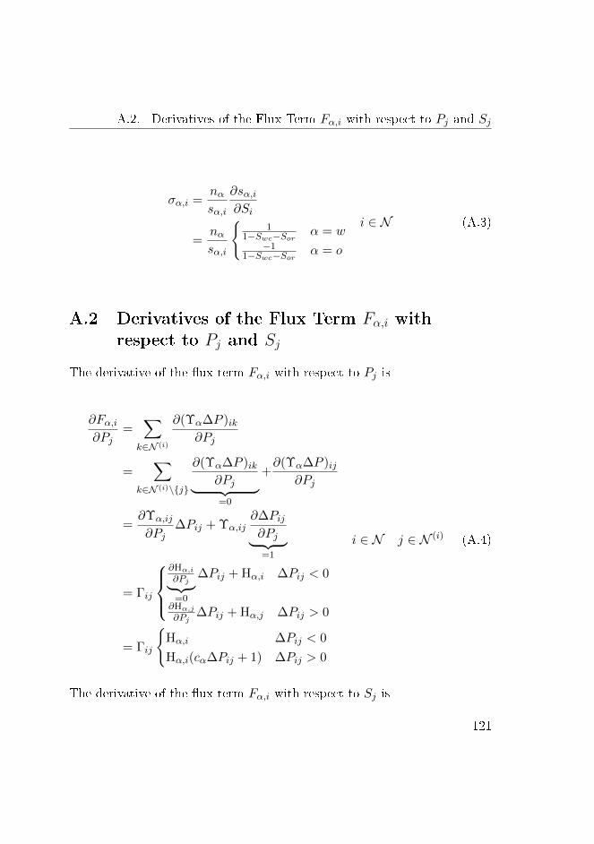
A.2. Derivatives of the Flux Term Fα,i with respect to Pj and Sj
σα,i =nαsα,i
∂sα,i∂Si
=nαsα,i
1
1−Swc−Sor α = w−1
1−Swc−Sor α = o
i ∈ N (A.3)
A.2 Derivatives of the Flux Term Fα,i withrespect to Pj and Sj
The derivative of the ux term Fα,i with respect to Pj is
∂Fα,i∂Pj
=∑
k∈N (i)
∂(Υα∆P )ik∂Pj
=∑
k∈N (i)\j
∂(Υα∆P )ik∂Pj︸ ︷︷ ︸=0
+∂(Υα∆P )ij
∂Pj
=∂Υα,ij
∂Pj∆Pij + Υα,ij
∂∆Pij∂Pj︸ ︷︷ ︸=1
= Γij
∂Hα,i∂Pj︸ ︷︷ ︸=0
∆Pij + Hα,i ∆Pij < 0
∂Hα,j∂Pj
∆Pij + Hα,j ∆Pij > 0
= Γij
Hα,i ∆Pij < 0
Hα,i(cα∆Pij + 1) ∆Pij > 0
i ∈ N j ∈ N (i) (A.4)
The derivative of the ux term Fα,i with respect to Sj is
121
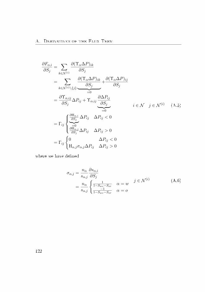
A. Derivatives of the Flux Term
∂Fα,i∂Sj
=∑
k∈N (i)
∂(Υα∆P )ik∂Sj
=∑
k∈N (i)\j
∂(Υα∆P )ik∂Sj︸ ︷︷ ︸=0
+∂(Υα∆P )ij
∂Sj
=∂Υα,ij
∂Sj∆Pij + Υα,ij
∂∆Pij∂Sj︸ ︷︷ ︸=0
= Γij
∂Hα,i∂Sj︸ ︷︷ ︸=0
∆Pij ∆Pij < 0
∂Hα,j∂Sj
∆Pij ∆Pij > 0
= Γij
0 ∆Pij < 0
Hα,jσα,j∆Pij ∆Pij > 0
i ∈ N j ∈ N (i) (A.5)
where we have dened
σα,j =nαsα,j
∂sα,i∂Sj
=nαsα,j
1
1−Swc−Sor α = w−1
1−Swc−Sor α = o
j ∈ N (i) (A.6)
122
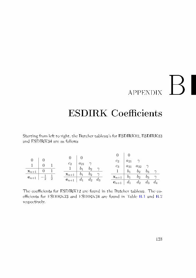
APPENDIX BESDIRK Coecients
Starting from left to right, the Butcher tableau's for ESDIRK12, ESDIRK23and ESDIRK34 are as follows
0 01 0 1
xn+1 0 1
en+1 −12
12
0 0c2 a21 γ1 b1 b2 γ
xn+1 b1 b2 γ
en+1 d1 d2 d3
0 0c2 a21 γc3 a31 a32 γ1 b1 b2 b3 γ
xn+1 b1 b2 b3 γ
en+1 d1 d2 d3 d4
The coecients for ESDIRK12 are found in the Butcher tableau. The co-ecients for ESDIRK23 and ESDIRK34 are found in Table B.1 and B.2respectively.
123
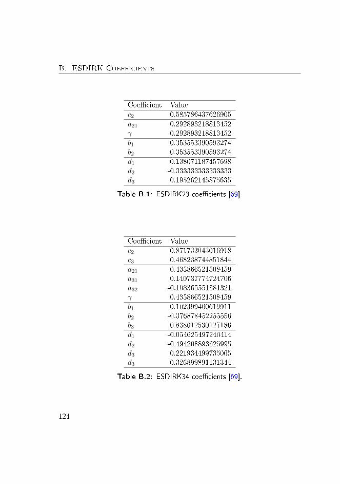
B. ESDIRK Coefficients
Coecient Value
c2 0.585786437626905
a21 0.292893218813452γ 0.292893218813452
b1 0.353553390593274b2 0.353553390593274
d1 0.138071187457698d2 -0.333333333333333d3 0.195262145875635
Table B.1: ESDIRK23 coecients [69].
Coecient Value
c2 0.871733043016918c3 0.468238744851844
a21 0.435866521508459a31 0.140737774724706a32 -0.108365551381321γ 0.435866521508459
b1 0.102399400619911b2 -0.376878452255556b3 0.838612530127186
d1 -0.054625497240414d2 -0.494208893625995d3 0.221934499735065d3 0.326899891131344
Table B.2: ESDIRK34 coecients [69].
124
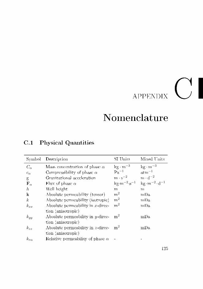
APPENDIX CNomenclature
C.1 Physical Quantities
Symbol Description SI Units Mixed Units
Cα Mass concentration of phase α kg ·m−3 kg ·m−3
cα Compressibility of phase α Pa−1 atm−1
g Gravitational acceleration m · s−2 m · d−2
Fα Flux of phase α kg·m−2·s−1 kg ·m−2 ·d−1
h Well height m mk Absolute permeability (tensor) m2 mDak Absolute permeability (isotropic) m2 mDakxx Absolute permeability in x-direc-
tion (anisotropic)m2 mDa
kyy Absolute permeability in y-direc-tion (anisotropic)
m2 mDa
kzz Absolute permeability in z-direc-tion (anisotropic)
m2 mDa
krα Relative permeability of phase α - -
125

C. Nomenclature
Symbol Description SI Units Mixed Units
krw Water end point relative perme-ability (krw = krw when 1−Sor ≤Sw ≤ 1)
- -
kro Oil end point relative permeabil-ity (kro = kro when 1 − Swc ≤So ≤ 1)
- -
nα Corey exponent of phase α - -Pα Pressure of phase α Pa atmP α Reference pressure of phase α
with density ρα
Pa atm
P bh Bottom hole pressure in producer Pa atmPcow Capillary pressure due to interfa-
cial tension between the oil phaseand the water phase
Pa atm
Qα Source/sink terms of phase α dueto injectors/producers
kg·m−3·s−1 kg ·m−3 ·d−1
Qinjα Source term (injector) of phase α kg·m−3·s−1 kg ·m−3 ·d−1
Qproα Sink term (producer) of phase α kg·m−3·s−1 kg ·m−3 ·d−1
qinj Volumetric water injection rate m3 · s−1 m3 · d−1
qinjα Mass injection rate of phase α kg · s−1 kg · d−1
qproα Mass production rate of phase α kg · s−1 kg · d−1
re Equivalent radius (radial dis-tance from the well at which thepressure obtained by the reser-voir model and the pressure ob-tained by the well model areequivalent)
m m
rw Well bore radius m mSα Saturation of phase α - -Swc Critical water saturation (water
does not to ow when 0 ≤ Sw ≤Swc)
- -
126
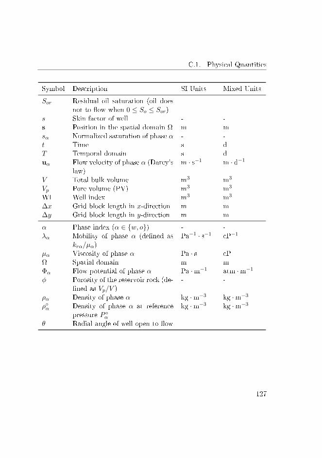
C.1. Physical Quantities
Symbol Description SI Units Mixed Units
Sor Residual oil saturation (oil doesnot to ow when 0 ≤ So ≤ Sor)
- -
s Skin factor of well - -s Position in the spatial domain Ω m msα Normalized saturation of phase α - -t Time s dT Temporal domain s duα Flow velocity of phase α (Darcy's
law)m · s−1 m · d−1
V Total bulk volume m3 m3
Vp Pore volume (PV) m3 m3
WI Well index m3 m3
∆x Grid block length in x-direction m m∆y Grid block length in y-direction m m
α Phase index (α ∈ w, o) - -λα Mobility of phase α (dened as
krα/µα)Pa−1 · s−1 cP−1
µα Viscosity of phase α Pa · s cPΩ Spatial domain m mΦα Flow potential of phase α Pa ·m−1 atm ·m−1
φ Porosity of the reservoir rock (de-ned as Vp/V )
- -
ρα Density of phase α kg ·m−3 kg ·m−3
ρα Density of phase α at referencepressure P α
kg ·m−3 kg ·m−3
θ Radial angle of well open to ow - -
127

C. Nomenclature
C.2 Commonly used Abbreviations
Abbreviation Description
BFGS Broyden-Fletcher-Goldfarb-ShannoBHP Bottom hole pressureDG-FEM Discontinuous Galerkin nite element methodDIRK Diagonally implicit Runge-KuttaEnKF Ensemble Kalman lterEOR Enhanced oil recoveryERK Explicit Runge-KuttaESDIRK Explicit singly diagonally implicit Runge-Kutta
ESDIRKkk Explicit singly diagonally implicit Runge-Kutta methodof order k with an embedded method of order k (ES-DIRK12, ESDIRK23 and ESDIRK34), see page 60
FDM Finite dierence methodFEM Finite element methodFIM Fully implicit methodFIRK Fully implicit Runge-KuttaFVM Finite volume methodIMEX Implicit-explicitIMPES Implicit pressure explicit saturationMPFA Multi-point ux approximationNMPC Nonlinear model predictive controlNPV Net present valueNR Newton-RaphsonODE Ordinary dierential equationPDE Partial dierential equationPI Proportional-integralPI97 Proportional-integral step size controller (original), see
page 71PI10 Proportional-integral step size controller (modied), see
page 71
128

C.2. Commonly used Abbreviations
Abbreviation Description
PV Pore volume Vp (void space of the reservoir rock contain-ing the reservoir uids)
SD Sigicant digitSDIRK Singly diagonally implicit Runge-KuttaSIM Sequential implicit methodSPU Single-point upstreamSQP Sequential quadratic programmingTPFA Two-point ux approximationWI Well index
129

APPENDIX DPaper A
Simulation of Subsurface Two-Phase Flowin an Oil Reservoir
Authors:
Carsten Völcker, John Bagterp Jørgensen, Per Grove Thomsen andErling Halfdan Stenby
Published in:
Proceedings of European Control Conference 2009 (ECC'09)Budapest, Hungary23-26 August 2009
131
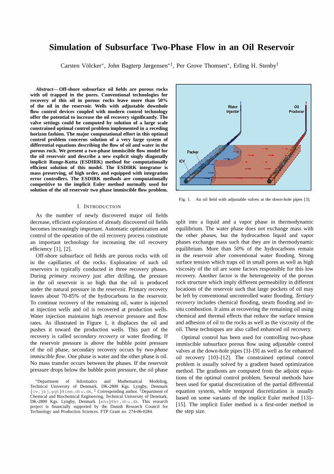
Simulation of Subsurface Two-Phase Flow in an Oil Reservoir
Carsten Volcker∗, John Bagterp Jørgensen∗‡, Per Grove Thomsen∗, Erling H. Stenby†
Abstract— Off-shore subsurface oil fields are porous rockswith oil trapped in the pores. Conventional technologies forrecovery of this oil in porous rocks leave more than 50%of the oil in the reservoir. Wells with adjustable downholeflow control devices coupled with modern control technologyoffer the potential to increase the oil recovery significantly. Thevalve settings could be computed by solution of a large scaleconstrained optimal control problem implemented in a recedinghorizon fashion. The major computational effort in this optimalcontrol problem concerns solution of a very large system ofdifferential equations describing the flow of oil and water in theporous rock. We present a two-phase immiscible flow model forthe oil reservoir and describe a new explicit singly diagonallyimplicit Runge-Kutta (ESDIRK) method for computationallyefficient solution of this model. The ESDIRK integrator ismass preserving, of high order, and equipped with integrationerror controllers. The ESDIRK methods are computationallycompetitive to the implicit Euler method normally used forsolution of the oil reservoir two phase immiscible flow problem.
I. I NTRODUCTION
As the number of newly discovered major oil fieldsdecrease, efficient exploration of already discovered oil fieldsbecomes increasingly important. Automatic optimization andcontrol of the operation of the oil recovery process constitutean important technology for increasing the oil recoveryefficiency [1], [2].
Off-shore subsurface oil fields are porous rocks with oilin the capillaries of the rocks. Exploration of such oilreservoirs is typically conducted in three recovery phases.During primary recovery just after drilling, the pressurein the oil reservoir is so high that the oil is producedunder the natural pressure in the reservoir. Primary recoveryleaves about 70-85% of the hydrocarbons in the reservoir.To continue recovery of the remaining oil, water is injectedat injection wells and oil is recovered at production wells.Water injection maintains high reservoir pressure and flowrates. As illustrated in Figure 1, it displaces the oil andpushes it toward the production wells. This part of therecovery is calledsecondary recoveryor water flooding. Ifthe reservoir pressure is above the bubble point pressureof the oil phase, secondary recovery occurs bytwo-phaseimmiscible flow. One phase is water and the other phase is oil.No mass transfer occurs between the phases. If the reservoirpressure drops below the bubble point pressure, the oil phase
∗Department of Informatics and Mathematical Modeling,Technical University of Denmark, DK-2800 Kgs. Lyngby, Denmarkcv,jbj,pgt @imm.dtu.dk , ‡ Corresponding author.†Department ofChemical and Biochemical Engineering, Technical University of Denmark,DK-2800 Kgs. Lyngby, Denmarkehs @kt.dtu.dk . This researchproject is financially supported by the Danish Research Council forTechnology and Production Sciences. FTP Grant no. 274-06-0284.
Fig. 1. An oil field with adjustable valves at the down-hole pipes [3].
split into a liquid and a vapor phase in thermodynamicequilibrium. The water phase does not exchange mass withthe other phases, but the hydrocarbon liquid and vaporphases exchange mass such that they are in thermodynamicequilibrium. More than 50% of the hydrocarbons remainin the reservoir after conventional water flooding. Strongsurface tension which traps oil in small pores as well as highviscosity of the oil are some factors responsible for this lowrecovery. Another factor is the heterogeneity of the porousrock structure which imply different permeability in differentlocations of the reservoir such that large pockets of oil maybe left by conventional uncontrolled water flooding.Tertiaryrecoveryincludes chemical flooding, steam flooding and in-situ combustion. It aims at recovering the remaining oil usingchemical and thermal effects that reduce the surface tensionand adhesion of oil to the rocks as well as the viscosity of theoil. These techniques are also called enhanced oil recovery.
Optimal control has been used for controlling two-phaseimmiscible subsurface porous flow using adjustable controlvalves at the down-hole pipes [3]–[9] as well as for enhancedoil recovery [10]–[12]. The constrained optimal controlproblem is usually solved by a gradient based optimizationmethod. The gradients are computed from the adjoint equa-tions of the optimal control problem. Several methods havebeen used for spatial discretization of the partial differentialequation system, while temporal discretization is usuallybased on some variants of the implicit Euler method [13]–[15]. The implicit Euler method is a first-order method inthe step size.

There is evidence, that high-order integration methodshave the potential to produce faster computation when ap-plied for temporal discretization of models describing multi-phase flows in porous media [16]. In this paper we developa model for two-phase immiscible flow in a porous medium.A finite volume method is used for spatial discretizationof the resulting system of partial differential equations. Anexplicit singly diagonally implicit Runge-Kutta (ESDIRK)method is used for temporal discretization. Newly developedESDIRK methods with mass preserving properties, error esti-mators and automatic step size controllers are presented. Theefficiency of the methods are demonstrated on simulationexamples.
II. 1-D IMENSIONAL MODEL
In this Section we describe a one-dimensional model fortwo-phase immiscible flow in a porous medium. This modelis important in its own right but also important for numericalstudies of solution procedures [17], [18]. The two phases areoil and water. The model consists of two partial differentialequations representing conservation of mass. Mass is trans-ported by convection at a velocity determined by Darcy’s law.Relative permeabilites are determined by a Corey expressionand we assume zero capillary pressure. The fluid densitiesare described by an equation of state relating the densitiesto pressure.
A. Conservation Equations and Boundary Conditions
Consider the one-dimensional spatial domainΩ = x ∈ R : 0 ≤ x ≤ L and the time domainT = t ∈ R : t ≥ 0. The boundary of the spatial domainis δΩ = x ∈ R : x = 0 ∧ x = L and the interior of thespatial domain isΩo = x ∈ R : 0 < x < L. The mass ofoil and water is conserved. SimilarlyδT = t ∈ R : t = 0andT o = t ∈ R : t > 0.
We consider a two-phase flow of oil and water withcomplete immiscibility. LetCw = Cw(t, x) and Co =Co(t, x) be the concentrations of water and oil (kg water/oilper volume reservoir) in the reservoir as function of timet ∈ T and positionx ∈ Ω. The mass balances for water andoil in the reservoir is expressed by the following system ofpartial differential equations
∂Cw
∂t= −∂Nw
∂x+ qw t ∈ T o, x ∈ Ωo (1a)
∂Co
∂t= −∂No
∂x+ qo t ∈ T o, x ∈ Ωo (1b)
Nw = Nw(t, x) andNo = No(t, x) are the fluxes of waterand oil through the porous medium. The source/sink terms ofwater and oil are denotedqw = qw(t, x) and qo = qo(t, x).They are used to describe the flow from injection wells andthe flow to production wells.
The initial concentrations of water and oil in the reservoirare specified
Cw(t, x) = Cw0(x) t ∈ δT, x ∈ Ω (2a)
Co(t, x) = Co0(x) t ∈ δT, x ∈ Ω (2b)
as well as the flux of water and oil at the boundaries
Nw(t, x) = 0 t ∈ T, x ∈ δΩ (3a)
No(t, x) = 0 t ∈ T, x ∈ δΩ (3b)
B. Constitutive Models
The concentrations of water and oil in the reservoir maybe expressed as
Cw = φρw(Pw)Sw (4a)
Co = φρo(Po)So (4b)
φ is the porosity of the reservoir rock. The porosity is thevolumetric fraction of void space that can be occupied by thereservoir fluids (water and oil). We assume the porosity to beconstant.ρw = ρw(Pw) andρo = ρo(Po) are the densities ofwater and oil. These densities depend on the water pressurePw and the oil pressurePo, respectively.Sw andSo are calledthe saturations of water and oil, respectively. They representthe volumetric fraction of water and oil in the void space.Consequently, as water and oil jointly fills the entire voidspace
Sw + So = 1 (5)
Water and oil are transported by convection through theporous medium. Therefore, the water and oil fluxes can beexpressed as
Nw = ρw(Pw)uw(Pw, Sw) (6a)
No = ρo(Po)uo(Po, So) (6b)
uw = uw(Pw, Sw) and uo = uo(Po, So) are the linearvelocities of each phase.
The flow through the porous medium is pressure drivenand can be expressed using Darcy’s law
uw = −kkrw(Sw)
µw
∂Pw
∂x(7a)
uo = −kkro(So)
µo
∂Po
∂x(7b)
k = k(x) denotes the permeability of the porous medium.The permeabilities depend only on the spatial position in thereservoir.µw andµo are the viscosities of oil and water. Therelative permeabilities of each phasekrw = krw(Sw) andkro = kro(So) are nonlinear functions of the saturation ofthe associated phase.
The relative permeabilities are approximated by the Coreyrelations
sw =Sw − Swc
1− Swc − Sor(8a)
so =So − Sor
1− Swc − Sor(8b)
krw(Sw) =
0 0 ≤ Sw ≤ Swc
krw0snww Swc < Sw < 1− Sor
krw0 1− Sor ≤ Sw ≤ 1
(8c)
kro(So) =
0 0 ≤ So ≤ Sor
kro0snoo Sor < So < 1− Swc
kro0 1− Swc ≤ So ≤ 1
(8d)

krw0, kro0, nw and no are determined experimentally foreach particular porous medium.Swc is the critical watersaturation andSor is the residual oil saturation.sw and soare the reduced saturations.
Assuming that the fluid compressibilitiescw and co areconstant over the pressure range of interest, the fluid densitiescan be expressed using the following equation of states
ρw = ρw0ecw(Pw−Pw0) (9a)
ρo = ρo0eco(Po−Po0) (9b)
ρw0 = ρw(Pw0) andρo0 = ρo(Po0) are the densities at thereference pressuresPw0 andPo0.
The pressure in the wetting fluid (the water in this case)is less than in the non-wetting fluid. The pressure differenceis given by the capillary pressure, which is assumed to be afunction of the water saturation
Pcow(Sw) = Po − Pw (10)
In highly permeable and highly porous media the capillaryeffects are small. In dense formations with very small poresthe capillary pressure introduces a diffusive term into (1)[19]. The irreducible saturationsSwc andSor can partly beexplained by the capillary effects in the porous medium, sothe capillary pressure is to some extend taken into accountthrough the relative permeabilities. In this model we assumezero capillary pressure
Pcow(Sw) = 0 (11)
C. Well Models
The injector and producer wells are all located at pointlocations. LetI denote an index set for the injectors andP denote an index set for the producers. Then the injectorsare located atxI,j for j ∈ I and the producers are locatedat xP,j for j ∈ P. Let δI,j = δ(x − xI,j) and δP,j =δ(x− xP,j) denote Dirac’s delta function.
Then the set of injector wells may be modeled as
qw = qw(t, x) = ρw(Pw)qjδI,j j ∈ I (12a)
qo = qo(t, x) = 0 j ∈ I (12b)
in which qj is the volumetric injection rate of water atinjection well j ∈ I. The set of producer wells are modeledas
qw = −αjwjρw(Pw)krw(Sw)
µw(Pw − Pwell,j)δP,j (13a)
qo = −αjwjρo(Po)kro(So)
µo(Po − Pwell,j)δP,j (13b)
in which j ∈ P. Pwell,j is the pressure at the well.αj ∈[0, 1] is the position of the control valve andwj is the well-index for production wellj ∈ P [13]–[15].
D. State Transformation
Let P = P (t, x) = Po(t, x) be the oil pressure andS =S(t, x) = Sw(t, x) be the water saturation. In the two-phaseimmiscible flow model (1)-(11), we may use(S, P ) as state
variables instead of(Cw, Co). (4), (5), (10) and (11) may beused to computeS andP givenCw andCo.
This imply that we may state the initial conditions (2) asinitial saturations and pressures
S(t, x) = S0(x) t ∈ δT, x ∈ Ω (14a)
P (t, x) = P0(x) t ∈ δT, x ∈ Ω (14b)
III. G ENERAL 3-DIMENSIONAL MODEL
Consider the time domainT = t ∈ R : t ≥ 0 and the
spatial domainΩ ⊂ R3. Let ∇ =[
∂∂x
∂∂y
∂∂z
]T. Using
the state variablesS = S(t, x, y, z) = Sw(t, x, y, z) andP =P (t, x, y, z) = Po(t, x, y, z) for t ∈ T and(x, y, z) ∈ Ω, wemay generalize the mass balances of the 1-D model to thegeneral 3-D model
∂Cw
∂t= −∇ ·Nw + qw t ∈ T o, (x, y, z) ∈ Ωo (15a)
∂Co
∂t= −∇ ·No + qo t ∈ T o, (x, y, z) ∈ Ωo (15b)
Nw =[Nw,x Nw,y Nw,z
]Tand No =[
No,x No,y No,z
]Tare 3-dimensional flux vectors
with the mass flux in each spatial direction as coordinates.The initial conditions with(S, P ) as state variables are
S(t, x, y, z) = S0(x, y, z) t ∈ δT, (x, y, z) ∈ Ω (16a)
P (t, x, y, z) = P0(x, y, z) t ∈ δT, (x, y, z) ∈ Ω (16b)
The zero net influx condition at the spatial boundary can beexpressed as
Nw(t, x, y, z) · n(x, y, z) = 0 t ∈ T, (x, y, z) ∈ δΩ (17a)
No(t, x, y, z) · n(x, y, z) = 0 t ∈ T, (x, y, z) ∈ δΩ (17b)
n(x, y, z) for (x, y, z) ∈ δΩ is a normal vector the boundaryδΩ.
The flux of water and oil is by convection. Therefore, theflux vectors are
Nw = ρw(Pw)uw (18a)
No = ρo(Po)uo (18b)
in whichuw anduo are linear velocities governed by Darcy’slaw
uw = −Kkrw(Sw)
µw(∇Pw − ρw(Pw)g∇z) (19a)
uo = −Kkro(So)
µo(∇Po − ρo(Po)g∇z) (19b)
with K = diag(kx, ky, kz) being a diagonal permeabilitymatrix. OftenK = kI.
The fluid and rock properties are determined in the samewas as for the 1-dimensional model. The source terms atinjection wells and the sink terms at production wells aredetermined by a trivial extension of Dirac’s delta-function tothe 3-dimensional case, i.e.δj = δ(x−xj)δ(y−yj)δ(z−zj).

IV. F INITE VOLUME DISCRETIZATION
In this section we present a method for spatial discretiza-tion of the two-phase immiscible flow problem. Using Gauss’divergence theorem, (15) may be expressed in integral form
∂
∂t
∫
Ω
CwdV = −∫
δΩ
(Nw · n)dS +
∫
Ω
qwdV (20a)
∂
∂t
∫
Ω
CodV = −∫
δΩ
(No · n)dS +
∫
Ω
qodV (20b)
n is an outward pointing normal vector on the boundary.The model integral form then consists of (20) along with theinitial conditions (16) and the boundary conditions (17). Inthis section we describe a finite volume method for spatialdiscretization of this model. For notational simplicity weconsider the equation
∂
∂t
∫
Ω
CdV = −∫
δΩ
(N · n)dS +
∫
Ω
qdV (21)
and the structured grid of finite volumes
Ωi,j,k = (x, y, z) ∈ R3 : xi− ≤ x ≤ xi+,yj− ≤ y ≤ yj+, zk− ≤ z ≤ zk+
(22)
with xi− =∑i−1
l=1 ∆xl, xi = xi− + 12∆xi, and xi+ =
xi−+∆xi. Similar definitions apply in they andz directions.Ωi,j,k is a finite volume with mid-point in(xi, yj , zk). δΩi,j,k
is the boundary of the finite volumeΩi,j,k. The concentrationin each control volumeΩi,j,k is obtained using
∂
∂t
∫
Ωi,j,k
CdV = −∫
δΩi,j,k
(N · n)dS +
∫
Ωi,j,k
qdV (23)
∀(i, j, k) along with the initial and boundary conditions. Theaccumulation term is
∂
∂t
∫
Ωi,j,k
CdV =dCi,j,k
dt(t)Vi,j,k (24)
with Vi,j,k = ∆xi∆yj∆zk. The flux term on the boundarymay be expressed as∫
δΩi,j,k
(N · n)dS =
Sx,j,k(Nx(t, xi+, yj , zk)−Nx(t, xi−, yj , zk))+
Sy,i,k(Ny(t, xi, yj+, zk)−Ny(t, xi, yj−, zk))+
Sz,i,j(Nz(t, xi, yj , zk+)−Nz(t, xi−, yj , zk−))
(25)
with Sx,j,k = ∆yj∆zk, Sy,i,k = ∆xi∆zk, andSz,i,j = ∆xi∆yj . Define the fluid transmissibilityζi,j,k =ρ(Pi,j,k)kr(Si,j,k)/µ. The fluxes in the x-direction are
Nx,i+,j,k = −kx,i+,j,kζi+,j,kPi+1,j,k − Pi,j,k
xi+1 − xi(26a)
Nx,i−,j,k = −kx,i−,j,kζi−,j,kPi,j,k − Pi−1,j,k
xi − xi−1(26b)
∆Nx,i,j,k = Nx,i+,j,k −Nx,i−,j,k (26c)
To have flux continuity across interfaces,kx,i+,j,k andkx,i−,j,k are computed using the harmonic average for thepermeabilities in the adjacent grid blocks
∆xi +∆xi−1
kx,i−,j,k=
∆xikx,i,j,k
+∆xi−1
kx,i−1,j,k(27a)
∆xi+1 +∆xikx,i+,j,k
=∆xi+1
kx,i+1,j,k+
∆xikx,i,j,k
(27b)
Due to the hyperbolic nature of the equation, the fluidtransmissibilities,ζi+,j,k and ζi−,j,k, are computed usingupstream information. The single point upstream scheme is
ζi+,j,k =
ζi+1,j,k Pi+1,j,k − Pi,j,k ≥ 0
ζi,j,k Pi+1,j,k − Pi,j,k < 0(28a)
ζi−,j,k =
ζi,j,k Pi,j,k − Pi−1,j,k ≥ 0
ζi−1,j,k Pi,j,k − Pi−1,j,k < 0(28b)
Similar expressions are derived for the fluxes in the y- and z-directions. In the z-direction we incorporate the gravity termin the flow direction test.
The source/sink term of (23) becomes∫
Ωi,j,k
qdV = qi,j,k(t)Vi,j,k (29)
Consequently, we may express the model (23) as a systemof ordinary differential equations in the form
dCi,j,k
dt= −
(∆Nx,i,j,k
∆xi+
∆Ny,i,j,k
∆yj+
∆Nz,i,j,k
∆zk
)
+ qi,j,k
(30)
V. ESDIRK
In this section we describe a method for temporal dis-cretization of the two-phase immiscible flow model.
A. New Differential Equation Model
Explicit Singly Diagonally Implicit Runge-Kutta (ES-DIRK) methods has previously been developed for systemof ordinary differential equations [20]–[23]
d
dtx(t) = f(t, x(t)) x(t0) = x0 (31)
and systems of index-1 differential algebraic equations [23],[24]
M(t, x(t))d
dtx(t) = f(t, x(t)) x(t0) = x0 (32)
While the spatially discretized model for the immiscible two-phase flow problem may be formulated as (32), the mainproblem with such a formulation is that it is not guaranteedto preserve mass upon discretization in time. This is amajor problem, as the differential equations was formulatedbased on conservation of mass. Process simulation problemsin general are based on conservation of mass, energy andmomentum. It is desirable to preserve such properties uponnumerical discretization in time.
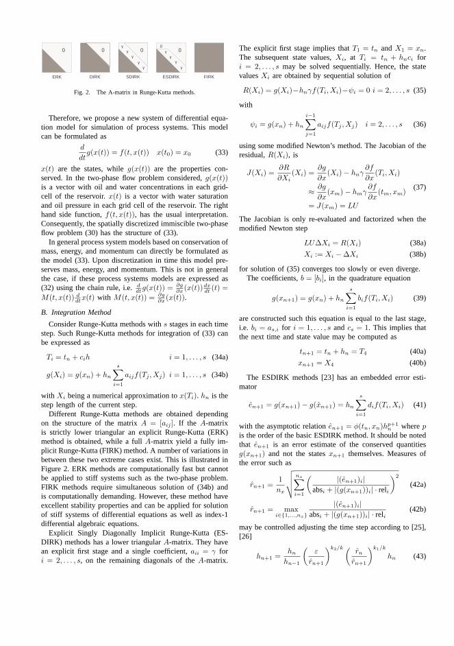
0 0 0 00
γγ
γγ
γγ
γγ
γ
ERK DIRK SDIRK ESDIRK FIRK
Fig. 2. The A-matrix in Runge-Kutta methods.
Therefore, we propose a new system of differential equa-tion model for simulation of process systems. This modelcan be formulated as
d
dtg(x(t)) = f(t, x(t)) x(t0) = x0 (33)
x(t) are the states, whileg(x(t)) are the properties con-served. In the two-phase flow problem considered,g(x(t))is a vector with oil and water concentrations in each grid-cell of the reservoir.x(t) is a vector with water saturationand oil pressure in each grid cell of the reservoir. The righthand side function,f(t, x(t)), has the usual interpretation.Consequently, the spatially discretized immiscible two-phaseflow problem (30) has the structure of (33).
In general process system models based on conservation ofmass, energy, and momentum can directly be formulated asthe model (33). Upon discretization in time this model pre-serves mass, energy, and momentum. This is not in generalthe case, if these process systems models are expressed as(32) using the chain rule, i.e.ddtg(x(t)) =
∂g∂x (x(t))
dxdt (t) =
M(t, x(t)) ddtx(t) with M(t, x(t)) = ∂g
∂x (x(t)).
B. Integration Method
Consider Runge-Kutta methods withs stages in each timestep. Such Runge-Kutta methods for integration of (33) canbe expressed as
Ti = tn + cih i = 1, . . . , s (34a)
g(Xi) = g(xn) + hn
s∑
i=1
aijf(Tj , Xj) i = 1, . . . , s (34b)
with Xi being a numerical approximation tox(Ti). hn is thestep length of the current step.
Different Runge-Kutta methods are obtained dependingon the structure of the matrixA = [aij ]. If the A-matrixis strictly lower triangular an explicit Runge-Kutta (ERK)method is obtained, while a fullA-matrix yield a fully im-plicit Runge-Kutta (FIRK) method. A number of variations inbetween these two extreme cases exist. This is illustrated inFigure 2. ERK methods are computationally fast but cannotbe applied to stiff systems such as the two-phase problem.FIRK methods require simultaneous solution of (34b) andis computationally demanding. However, these method haveexcellent stability properties and can be applied for solutionof stiff systems of differential equations as well as index-1differential algebraic equations.
Explicit Singly Diagonally Implicit Runge-Kutta (ES-DIRK) methods has a lower triangularA-matrix. They havean explicit first stage and a single coefficient,aii = γ fori = 2, . . . , s, on the remaining diagonals of theA-matrix.
The explicit first stage implies thatT1 = tn andX1 = xn.The subsequent state values,Xi, at Ti = tn + hnci fori = 2, . . . , s may be solved sequentially. Hence, the statevaluesXi are obtained by sequential solution of
R(Xi) = g(Xi)−hnγf(Ti, Xi)−ψi = 0 i = 2, . . . , s (35)
with
ψi = g(xn) + hn
i−1∑
j=1
aijf(Tj , Xj) i = 2, . . . , s (36)
using some modified Newton’s method. The Jacobian of theresidual,R(Xi), is
J(Xi) =∂R
∂Xi(Xi) =
∂g
∂x(Xi)− hnγ
∂f
∂x(Ti, Xi)
≈ ∂g
∂x(xm)− hmγ
∂f
∂x(tm, xm)
= J(xm) = LU
(37)
The Jacobian is only re-evaluated and factorized when themodified Newton step
LU∆Xi = R(Xi) (38a)
Xi := Xi −∆Xi (38b)
for solution of (35) converges too slowly or even diverge.The coefficients,b = [bi], in the quadrature equation
g(xn+1) = g(xn) + hn
s∑
i=1
bif(Ti, Xi) (39)
are constructed such this equation is equal to the last stage,i.e. bi = as,i for i = 1, . . . , s and cs = 1. This implies thatthe next time and state value may be computed as
tn+1 = tn + hn = T4 (40a)
xn+1 = X4 (40b)
The ESDIRK methods [23] has an embedded error esti-mator
en+1 = g(xn+1)− g(xn+1) = hn
s∑
i=1
dif(Ti, Xi) (41)
with the asymptotic relationen+1 = φ(tn, xn)hp+1n wherep
is the order of the basic ESDIRK method. It should be notedthat en+1 is an error estimate of the conserved quantitiesg(xn+1) and not the statesxn+1 themselves. Measures ofthe error such as
rn+1 =1
nx
√√√√nx∑
i=1
( |(en+1)i|absi + |(g(xn+1))i| · reli
)2
(42a)
rn+1 = maxi∈1,...,nx
|(en+1)i|absi + |(g(xn+1))i| · reli
(42b)
may be controlled adjusting the time step according to [25],[26]
hn+1 =hnhn−1
(ε
rn+1
)k2/k ( rnrn+1
)k1/k
hn (43)
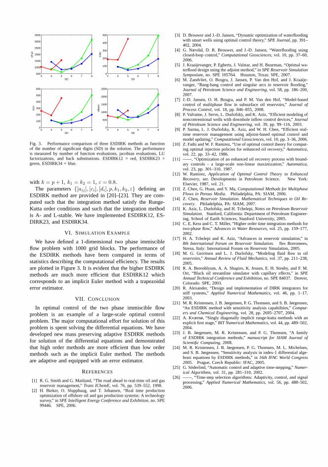
3 4 5 6 7 8500
1000
1500
2000
2500
3000
3500
SD
nFun
3 4 5 6 7 80
100
200
300
400
500
SD
nJac
3 4 5 6 7 80
100
200
300
400
500
600
SD
nLU
3 4 5 6 7 80
500
1000
1500
2000
2500
SD
nBac
k
Fig. 3. Performance comparison of three ESDIRK methods as functionof the number of significant digits (SD) in the solution. The performanceis measured by number of function evaluations, jacobian evaluations, LUfactorizations, and back substitutions. ESDIRK12 = red, ESDIRK23 =green, ESDIRK34 = blue.
with k = p+ 1, k1 = k2 = 1, ε = 0.8.The parameters[aij ], [ci], [di], p, k1, k2, ε defining an
ESDIRK method are provided in [20]–[23]. They are com-puted such that the integration method satisfy the Runge-Kutta order conditions and such that the integration methodis A- and L-stable. We have implemented ESDIRK12, ES-DIRK23, and ESDIRK34.
VI. SIMULATION EXAMPLE
We have defined a 1-dimensional two phase immiscibleflow problem with 1000 grid blocks. The performance ofthe ESDIRK methods have been compared in terms ofstatistics describing the computational efficiency. The resultsare plotted in Figure 3. It is evident that the higher ESDIRKmethods are much more efficient that ESDIRK12 whichcorresponds to an implicit Euler method with a trapezoidalerror estimator.
VII. C ONCLUSION
In optimal control of the two phase immiscible flowproblem is an example of a large-scale optimal controlproblem. The major computational effort for solution of thisproblem is spent solving the differential equations. We havedeveloped new mass preserving adaptive ESDIRK methodsfor solution of the differential equations and demonstratedthat high order methods are more efficient than low ordermethods such as the implicit Euler method. The methodsare adaptive and equipped with an error estimator.
REFERENCES
[1] R. G. Smith and G. Maitland, “The road ahead to real-time oil and gasreservoir management,”Trans IChemE, vol. 76, pp. 539–552, 1998.
[2] H. Bieker, O. Slupphaug, and T. Johansen, “Real time productionoptimization of offshore oil and gas production systems: A technologysurvey,” inSPE Intelligent Energy Conference and Exhibition, no. SPE99446. SPE, 2006.
[3] D. Brouwer and J.-D. Jansen, “Dynamic optimization of waterfloodingwith smart wells using optimal control theory,”SPE Journal, pp. 391–402, 2004.
[4] G. Nævdal, D. R. Brouwer, and J.-D. Jansen, “Waterflooding usingclosed-loop control,”Computational Geosciences, vol. 10, pp. 37–60,2006.
[5] J. Kraaijevanger, P. Egberts, J. Valstar, and H. Buurman, “Optimal wa-terflood design using the adjoint method,” inSPE Reservoir SimulationSymposium, no. SPE 105764. Houston, Texas: SPE, 2007.
[6] M. Zandvliet, O. Bosgra, J. Jansen, P. Van den Hof, and J. Kraaije-vanger, “Bang-bang control and singular arcs in reservoir flooding,”Journal of Petroleum Science and Engineering, vol. 58, pp. 186–200,2007.
[7] J.-D. Jansen, O. H. Bosgra, and P. M. Van den Hof, “Model-basedcontrol of multiphase flow in subsurface oil reservoirs,”Journal ofProcess Control, vol. 18, pp. 846–855, 2008.
[8] P. Valvatne, J. Serve, L. Durlofsky, and K. Aziz, “Efficient modeling ofnonconventional wells with downhole inflow control devices,”Journalof Petroleum Science and Engineering, vol. 39, pp. 99–116, 2003.
[9] P. Sarma, L. J. Durlofsky, K. Aziz, and W. H. Chen, “Efficient real-time reservoir management using adjoint-based optimal control andmodel updating,”Computational Geosciences, vol. 10, pp. 3–36, 2006.
[10] Z. Fathi and W. F. Ramirez, “Use of optimal control theory for comput-ing optimal injection policies for enhanced oil recovery,”Automatica,vol. 22, pp. 33–42, 1986.
[11] ——, “Optimization of an enhanced oil recovery process with bound-ary controls - a large-scale non-linear maximization,”Automatica,vol. 23, pp. 301–310, 1987.
[12] W. Ramirez, Application of Optimal Control Theory to EnhancedRecovery, ser. Developments in Petroleum Science. New York:Elsevier, 1987, vol. 21.
[13] Z. Chen, G. Huan, and Y. Ma,Computational Methods for MultiphaseFlows in Porous Media. Philadelphia, PA: SIAM, 2006.
[14] Z. Chen,Reservoir Simulation. Mathematical Techniques in Oil Re-covery. Philadelphia, PA: SIAM, 2007.
[15] K. Aziz, L. Durlofsky, and H. Tchelepi,Notes on Petroleum ReservoirSimulation. Stanford, California: Department of Petroleum Engineer-ing, School of Earth Sciences, Stanford University, 2005.
[16] C. E. Kess and C. T. Miller, “Higher order time integration methods fortwo-phase flow,”Advances in Water Resources, vol. 25, pp. 159–177,2002.
[17] H. A. Tchelepi and K. Aziz, “Advances in reservoir simulation,” in8th International Forum on Reservoir Simulation. Iles Borromees,Stresa, Italy: International Forum on Reservoir Simulation, 2005.
[18] M. G. Gerritsen and L. J. Durlofsky, “Modeling fluid flow in oilreservoirs,”Annual Review of Fluid Mechanics, vol. 37, pp. 211–238,2005.
[19] R. A. Berenblyum, A. A. Shapiro, K. Jessen, E. H. Stenby, and F. M.Orr, “Black oil streamline simulator with capillary effects,” inSPEAnnual Technical Conference and Exhibition, no. SPE 84037. Denver,Colorado: SPE, 2003.
[20] R. Alexander, “Design and implementation of DIRK integrators forstiff systems,” Applied Numerical Mathematics, vol. 46, pp. 1–17,2003.
[21] M. R. Kristensen, J. B. Jørgensen, P. G. Thomsen, and S. B. Jørgensen,“An ESDIRK method with sensitivity analysis capabilities,”Comput-ers and Chemical Engineering, vol. 28, pp. 2695–2707, 2004.
[22] A. Kværnø, “Singly diagonally implicit runge-kutta methods with anexplicit first stage,”BIT Numerical Mathematics, vol. 44, pp. 489–502,2004.
[23] J. B. Jørgensen, M. R. Kristensen, and P. G. Thomsen, “A familyof ESDIRK integration methods,”manuscript for SIAM Journal ofScientific Computing, 2008.
[24] M. R. Kristensen, J. B. Jørgensen, P. G. Thomsen, M. L. Michelsen,and S. B. Jørgensen, “Sensitivity analysis in index-1 differential alge-braic equations by ESDIRK methods,” in16th IFAC World Congress2005. Prague, Czech Republic: IFAC, 2005.
[25] G. Soderlind, “Automatic control and adaptive time-stepping,”Numer-ical Algorithms, vol. 31, pp. 281–310, 2002.
[26] ——, “Time-step selection algorithms: Adaptivity, control, and signalprocessing,”Applied Numerical Mathematics, vol. 56, pp. 488–502,2006.


APPENDIX EPaper B
Adaptive Stepsize Control in Implicit Runge-Kutta Methodsfor Reservoir Simulation
Authors:
Carsten Völcker, John Bagterp Jørgensen, Per Grove Thomsen andErling Halfdan Stenby
Published in:
Proceedings of 9th International Symposium on Dynamics and Controlof Process Systems (DYCOPS 2010)Leuven, Belgium5-7 July 2010
139

Adaptive Stepsize Control in Implicit
Runge-Kutta Methods for Reservoir
Simulation ?
Carsten Volcker ∗ John Bagterp Jørgensen ∗
Per Grove Thomsen ∗ Erling Halfdan Stenby ∗∗
∗ Department of Informatics and Mathematical Modeling, TechnicalUniversity of Denmark, DK-2800 Kgs. Lyngby, Denmark (e-mail:
cv,jbj,[email protected])∗∗ Department of Chemical and Biochemical Engineering, TechnicalUniversity of Denmark, DK-2800 Kgs. Lyngby, Denmark (e-mail:
Abstract: This paper concerns predictive stepsize control applied to high order methods fortemporal discretization in reservoir simulation. The family of Runge-Kutta methods is presentedand in particular the explicit singly diagonally implicit Runge-Kutta (ESDIRK) methods aredescribed. A predictive stepsize adjustment rule based on error estimates and convergencecontrol of the integrated iterative solver is presented. We try to improve the predictive stepsizecontrol by smoothing the stepsize sequence through combining the control of error with thecontrol of convergence.
Keywords: Reservoir simulation, Runge-Kutta methods, convergence control, stepsize selection.
1. INTRODUCTION
Reservoir simulators are computer programs that solvethe equations for heat and mass flow in porous media.Numerical integration is one of the basic steps involved inthe simulation process. The number and type of equationsto be solved depend on the geological characteristics of thereservoir, the characteristics of the oil and the oil recoveryprocess to be modeled. Choosing the appropriate methodof integration involves deciding on factors such as theorder of the integration scheme, stability properties andconcern on computational efficiency. ESDIRK methodshave been applied successfully for solution of convection-diffusion-reaction problems, see Kennedy and Carpenter(2003). This class of methods is computationally efficient,and both A- and L-stable and stiffly accurate ESDIRKmethods of various order with an embedded method forerror estimation have been derived by Kværnø (2004) andJørgensen et al. (2008). In addition, a robust adaptivestepsize selection is essential to an efficient numericalintegration. An adaptive stepsize selection aims to keepthe error estimate bounded i.e. close to a user-specifiedtolerance by adjusting the timestep. Gustafsson (1992)suggested a strategy for stepsize selection based on therigorous error estimates provided by embedded Runge-Kutta methods.We have applied the controller by Gustafsson and Soder-lind (1997) to three different ESDIRK methods used forsolving a two-phase reservoir model. Although the controlstrategy has proven efficient we observed that certain steps
? This research project is financially supported by the DanishResearch Council for Technology and Production Sciences. FTPGrant no. 274-06-0284.
were rejected due to irregularities in the stepsize selection.We found that a different interaction between the error andthe convergence control in the stepsize selection processmay solve this problem. The idea is to combine the controlof error with control of convergence in the inner iterationsin a simple logic that minimizes the number of rejectedsteps and thereby improves the efficiency.
2. DIFFERENTIAL EQUATION MODEL
In this section we briefly outline the two-phase flow prob-lem and we present the typical formulation of a system ofordinary differential equations (ODE) based on conserva-tion laws.
2.1 The two-phase flow problem
We consider immiscible two-phase flow of oil and water inporous media. Let Po = Po(t, x) be the pressure of oil andSw = Sw(t, x) be the saturation of water, as function oftime t ≥ 0 and position x ⊂ R2, and let Cw = Cw(Po, Sw)and Co = Co(Po, Sw) be the mass concentrations of waterand oil respectively. Then the mass balances for water andoil in the reservoir is expressed by the following system ofpartial differential equations
∂
∂tCw= −∇ · Fw +Qw (1a)
∂
∂tCo = −∇ · Fo +Qo (1b)
Fw = Fw(Po, Sw) and Fo = Fo(Po, Sw) are the fluxes ofwater and oil through the porous media. The source/sink
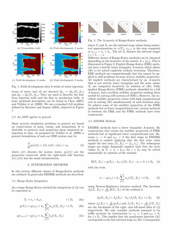
x [m]
y [m
]
0 100 200 300 4000
100
200
300
400
2000
4000
6000
8000
10000
12000
(a) Permeability field.
x [m]
y [m
]
0 100 200 300 4000
100
200
300
400
0
0.2
0.4
0.6
(b) Field development, 3 weeks.
x [m]
y [m
]
0 100 200 300 4000
100
200
300
400
0
0.2
0.4
0.6
(c) Field development, 6 weeks.
x [m]
y [m
]
0 100 200 300 4000
100
200
300
400
0.1
0.2
0.3
0.4
0.5
0.6
0.7
(d) Field development, 9 weeks.
Fig. 1. Field development after 9 weeks of water injection.
terms of water and oil are denoted Qw = Qw(Po, Sw)and Qo = Qo(Po, Sw). They are used to describe the flowfrom injection wells and the flow to production wells. Amore profound description can be found in Chen (2007)and Volcker et al. (2009). We use a standard 2-D problemdefined by Brouwer and Jansen (2004), depicted in Figure1.
2.2 An ODE system in general
Many process simulation problems in general are basedon conservation of mass, energy and momentum. It isdesirable to preserve such properties upon numerical in-tegration in time. As proposed by Volcker et al. (2009) ageneral formulation of such an ODE system may be
d
dtg(x(t)) = f(t, x(t)) x(t0) = x0 (2)
where x(t) denotes the system states, g(x(t)) are theproperties conserved, while the right-hand side functionf(t, x(t)) has the usual interpretation.
3. INTEGRATION METHODS
In this section different classes of Runge-Kutta methodsare outlined. In particular ESDIRKmethods are described.
3.1 Runge-Kutta Integration
An s-stage Runge-Kutta method for integration of (2) canbe expressed as
Ti = tn + hnci i ∈ S1 (3a)
g(Xi) = g(xn) + hn
s∑
j=1
aijf(Tj , Xj) i ∈ S1 (3b)
g(xn+1) = g(xn) + hn
s∑
j=1
bjf(Tj , Xj) (3c)
0 0 0 00
γγ
γγ
γγ
γγ
γ
ERK DIRK SDIRK ESDIRK FIRK
Fig. 2. The A-matrix of Runge-Kutta methods.
where Ti and Xi are the internal stage values being numer-ical approximations to x(Ti). xn+1 is the step computedat tn+1 = tn + hn. The set Si denotes the internal stagesi, i+ 1, . . . , s.Different classes of Runge-Kutta methods can be obtaineddepending on the structure of the matrix A = [aij ]. This isillustrated in Figure 2. Explicit Runge-Kutta (ERK) meth-ods have a strictly lower triangular A-matrix which allows(3b) to be solved explicitly without iterations. Therefore,ERK methods are computationally fast but cannot be ap-plied to stiff problems because of poor stability properties.All implicit methods are characterized by an A-matrixthat is not strictly lower triangular and the state valuesXi are computed iteratively by solution of (3b). Fullyimplicit Runge-Kutta (FIRK) methods, identified by a fullA-matrix, have excellent stability properties making themusefull for solving stiff systems of ODE’s. However, the ex-cellent stability properties comes with high computationalcost in solving (3b) simultaneously at each iteration step.To achieve some of the stability properties of the FIRKmethods but at lower computational cost, various methodsin between the ERK and the FIRK methods have beenconstructed.
3.2 ESDIRK Methods
ESDIRK methods have a lower triangular A-matrix. Byconstruction they retain the stability properties of FIRKmethods but at significant lower computational cost. Be-cause c1 = 0 and a11 = 0 the first stage in ESDIRKmethods is explicit implying that the first state valueequals the last step (T1, X1) = (tn, xn). The subsequentstages are singly diagonally implicit such that the statevalues Xi at Ti = tn + hnci for i ∈ S2 may be solvedsequentially by solution of the residual
R(Ti, Xi) = g(Xi)− hnγf(Ti, Xi)− ψi = 0 i ∈ S2 (4)
with the term
ψi = g(xn) + hn
i−1∑
j=1
aijf(Tj , Xj) i ∈ S2 (5)
using Newton-Raphson’s iterative method. The JacobianJR(Ti, Xi) =
∂∂Xi
R(Ti, Xi) of the residual is
JR(Ti, Xi) = Jg(Xi)− hnγJf (Ti, Xi) i ∈ S2 (6)
where Jg(Xi) =d
dXig(Xi) and Jf (Ti, Xi) =
∂∂Xi
f(Ti, Xi)
are the Jacobiants of the right- and left-hand sides of (2)respectively. We only consider methods assumed to bestiffly accurate by construction i.e. cs = 1 and asj = bjfor j ∈ S1. This implies that the quadrature function (3c)corresponds to the last internal stage in (3b). Consequently
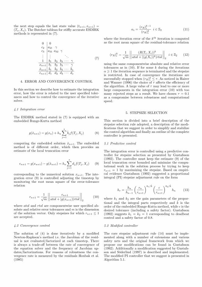
the next step equals the last state value (tn+1, xn+1) =(Ts, Xs). The Butcher tableau for stiffly accurate ESDIRKmethods is represented in (7).
0 0c2 a21 γc3 a31 a32 γ...
.... . .
1 b1 b2 b3 · · · γxn+1 b1 b2 b3 · · · γxn+1 b1 b2 b3 · · · bsen+1 d1 d2 d3 · · · ds
(7)
4. ERROR AND CONVERGENCE CONTROL
In this section we describe how to estimate the integrationerror, how the error is related to the user specified toler-ances and how to control the convergence of the iterativesolver.
4.1 Integration error
The ESDIRK method stated in (7) is equipped with anembedded Runge-Kutta method
g(xn+1) = g(xn) + hn
s∑
j=1
bjf(Tj , Xj) (8)
computing the embedded solution xn+1. The embeddedmethod is of different order, which then provides anestimate of the local truncation error
en+1 = g(xn+1)− g(xn+1) = hn
s∑
j=1
djf(Tj , Xj) (9)
corresponding to the numerical solution xn+1. The inte-gration error (9) is controlled adjusting the timestep bymonitoring the root mean square of the error-tolerancerelation
rn+1 =1√m
∣∣∣∣∣∣∣∣
en+1
atol + |g(xn+1)|rtol
∣∣∣∣∣∣∣∣2
(10)
where atol and rtol are componentwise user specified ab-solute and relative error tolerances and m is the dimensionof the solution vector. Only stepsizes for which rn+1 ≤ 1are accepted.
4.2 Convergence control
The solution of (4) is done iteratively by a modifiedNewton-Raphson’s method i.e. the Jacobian of the resid-ual is not evaluated/factorized at each timestep. Thereis always a trade-off between the rate of convergence ofthe equation solver and the frequency of Jacobian up-dates/factorizations. For reasons of robustness the con-vergence rate is measured by the residuals Houbak et al.(1985)
αi =(rR)
k−1i
(rR)kii ∈ S2 (11)
where the iteration error of the kth iteration is computedas the root mean square of the residual-tolerance relation
(rR)ki =
1√m
∣∣∣∣∣∣∣∣
(R(Ti, Xi))k
atol + |(g(Xi))k|rtol
∣∣∣∣∣∣∣∣2
i ∈ S2 (12)
using the same componentwise absolute and relative errortolerances as in (10). If for some k during the iterationsα ≥ 1 the iteration sequence is terminated and the stepsizeis restricted. In case of convergence the iterations aresuccessfully stopped when (rR)
ki ≤ τ . As noticed in Hairer
and Wanner (1996) the choice of τ affects the efficiency ofthe algorithm. A large value of τ may lead to one or morelarge components in the integration error (10) with toomany rejected steps as a result. We have chosen τ = 0.1as a compromise between robustness and computationalspeed.
5. STEPSIZE SELECTION
This section is divided into a brief description of thestepsize selection rule adopted, a description of the modi-fications that we suggest in order to simplify and stabilizethe control algorithm and finally an outline of the completecontroller is presented.
5.1 Predictive control
The integration error is controlled using a predictive con-troller for stepsize selection as presented by Gustafsson(1992). The controller must keep the estimate (9) of thelocal truncation error bounded and minimize the compu-tational work in the solution process by trying to keeprn+1 = 1 by maximizing the stepsize. Based on empiri-cal evidence Gustafsson (1992) suggested a proportionalintegral (PI) stepsize adjustment rule on the form
hr =hnhn−1
(rnrn+1
)k1/k ( ε
rn+1
)k2/k
hn (13)
where k1 and k2 are the gain parameters of the propor-
tional and the integral parts respectively and k is theorder of the embedded Runge-Kutta method, while ε is thedesired tolerance (including a safety factor). Gustafsson(1992) suggests k1 = k2 = 1 corresponding to deadbeatcontrol and a safety factor of 0.8.
5.2 Modified controller
The core stepsize adjustment rule (14) must be imple-mented along with a number of extensions and varioussafety nets and the original framework from which wepropose our modifications can be found in Gustafsson(1992). Additionally a modification suggested by Gustafs-son and Soderlind (1997) is described and implemented.The modified PI controller that we suggest is presented inAlgorithm 5.1.
Since we are only considering stiffly accurate methodsthe order reduction for stiff systems can be avoided, seeProthero and Robinson (1974). Consequently the strategy
described by Gustafsson (1992) for estimating k aftersuccessive rejects can be omitted. This does not makeany noticeable change in the controller performance butsimplifies the algorithm a great deal.Besides the frequency of Jacobian updates/factorizationsthe stepsize is the only available control variable affectingthe convergence rate of the equation solver. In order toassure convergence in the equation solver the stepsize hasto be restrained in some situations. If convergence is tooslow i.e. if α > αref Gustafsson (1992) suggest the stepsizeto be chosen as
hα =αref
αhn (14)
to obtain α = αref in the next step. The stepsize suggestedby (15) must be coordinated with the requirements fromthe error control. If α > αref the stepsize in Gustafsson(1992) is implemented as
hn+1 = min(hr, hα) (15)
restraining the stepsize if hα < hr. The strategy adoptedby (15) and (16) may be too aggressive in the sense thatthe corresponding error estimate (10) becomes very lowcompared to ε. Hence the subsequent stepsize estimatedby the asymptotic controller
hr =
(ε
rn+1
)1/k
hn (16)
will be too large making the error estimate and thereby thestepsize fluctuate wildly. We try to avoid this by modifying(15) to
hα =(αref
α
)1/khn (17)
which means that the deviation of the convergence ratefrom αref is not necessarily corrected in one step. If a stephas been rejected and restricted by slow convergence, thenin combination (17) is filtered by the relation between theprevious accepted step and the current accepted step
hr =hnhn−1
(ε
rn+1
)1/k
hn (18)
which further reduces the stepsize following a convergencerestricted step. If the current step is accepted we neglectthe condition α > αref on (16). In addition (14) is al-ways used estimating the next stepsize, whenever a stepis accepted. Consequently we allow the convergence of theequation solver to gain more influence on the stepsize se-lection. While Gustafsson (1992) suggests 0.2 . αref . 0.5as set-points for the convergence rate we chose αref = 0.6.This value favours robustness and a minimum amount ofwork needed to complete the integration fairly equal.Slow convergence in the equation solver and in particularrejected steps because of convergence failure is very costly.
This can to some extend be controlled by the stepsize butalso by the frequency of Jacobian updates/factorizations.Considering (6) we see that stepsize changes invokes arefactorization of the Jacobian but not necessarily a Ja-cobian reevaluation - if on the other hand the Jacobian isupdated a factorization is always called for. Good conver-gence can be obtained by both updating and factorizingthe Jacobian at every stepsize change. For large systemsthough this may be the dominating part of the computa-tions and large savings can be made by utilizing a strat-egy for reusing the same Jacobian for several timesteps.Gustafsson (1992) monitors the relative stepsize changesince the last factorization was done and suggests
|hn+1 − hLU |/hLU > αLU (19)
as a refactorization strategy. The strategy is preventive inthe sense that it tries to avoid convergence failures by fac-torizing whenever planning to do a stepsize change that islikely to jeopardize convergence. Should poor convergencebe experienced despite a factorization based on currentdata, say α > αJac, then a reevaluation of the Jacobianis called for. Gustafsson and Soderlind (1997) suggests thecombination
α− |hn+1 − hLU |/hLU > αJac (20)
as decision for when to compute a new Jacobian. Besidesmonitoring the convergence rate of the equation solver thisstrategy also trades Jacobian updates with factorizationsand function evaluations. The value of αref sets an upperlimit on αJac and αLU , see Gustafsson (1992). In the two-phase flow problem the administration of the Jacobianis expensive compared to one iteration. This argues forlarge values of αJac and αLU . To be more specific it ismore costly to update the Jacobian than factorizing it,consequently we have chosen αJac = 0.5 and αLU = 0.3.Because of the large value of αJac we allow a fairly largemaximum number of iterations in the equation solver,setting kmax = 20.
5.3 The complete controller
The complete modified PI controller for an implicit Runge-Kutta method is outlined in Algorithm 5.1. The controllerincludes three main parts:
• A stepsize selection rule based on both the error-tolerance relation and the convergence of the equationsolver.
• An update/factorization strategy for the Jacobianthat supervises the convergence and the iterationerror of the equation solver.
• A strategy for handling convergence failures.
6. CHOICE OF METHODS
In this section the two-phase flow problem is used as abenchmark. We compare and discuss the performance ofthe controller by Gustafsson and Soderlind (1997) andthe controller suggested in Algorithm 5.1 when applied tothree different ESDIRK methods.In this section ESDIRKkk refers to an ESDIRK method of
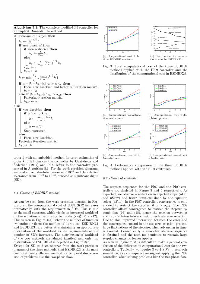
Algorithm 5.1: The complete modified PI controller foran implicit Runge-Kutta method.
if iterations converged then
hr ←(εr
)1/kh
if step accepted thenif step restricted then
hr ← hhacc
hrelse
hr ← hhacc
(racc
r
)1/khr
racc ← rhacc ← h
h← min
(hr,(αref
α
)1/kh
)
if α− |h− hLU |/hLU > αJac thenForm new Jacobian and factorize iteration matrix.hLU ← h
else if |h− hLU |/hLU > αLU thenFactorize iteration matrix.hLU ← h
elseif new Jacobian then
if α > αref then
h←(αref
α
)1/kh
elseh← h/2
Step restricted.else
Form new Jacobian.Factorize iteration matrix.hLU ← h
order k with an embedded method for error estimation oforder k. PI97 denotes the controller by Gustafsson andSoderlind (1997) and PI09 refers to the controller pre-sented in Algorithm 5.1. For the work-precision diagramswe used a fixed absolute tolerance of 10−8 and the relativetolerances from 10−2 to 10−8, denoted as significant digits(SD).
6.1 Choice of ESDIRK method
As can be seen from the work-precision diagram in Fig-ure 3(a), the computational cost of ESDIRK12 increasesdramatically with the requirement in SD’s. This is dueto the small stepsizes, which yields an increased workloadof the equation solver trying to retain (rR)
ki ≤ τ (12).
This is seen in Figure 4(a), where the number of functionevaluations reflects the number of iterations. ESDIRK23and ESDIRK34 are better at maintaining an appropriatedistribution of the workload as the requirements of thenumber in SD’s increases. The distribution of workloadof the two methods are almost identical and only thedistribution of ESDIRK23 is depicted in Figure 3(b).Except for SD = 2 we observe from the work-precisiondiagram of the three methods, that ESDIRK23 is the mostcomputationally efficient method for temporal discretiza-tion of problems like the two-phase flow.
2 3 4 5 6 7 810
0
101
102
103
SD
tES
DIR
K [s
]
ESDIRK12ESDIRK23ESDIRK34
(a) Computational cost of thethree ESDIRK methods.
2 3 4 5 6 7 80
10
20
30
40
50
60
70
80
90
100
SD
Dis
trib
utio
n of
com
p. ti
me
[%]
Function evaluations
Jacobian updates
LU factorizations
Backward substitutions
Other comptations
(b) Distribution of computa-tional cost in ESDIRK23.
Fig. 3. Total computational cost of the three ESDIRKmethods applied with the PI09 controller and thedistribution of the computational cost in ESDIRK23.
2 3 4 5 6 7 810
−1
100
101
102
103
SD
tFun
[s]
ESDIRK12ESDIRK23ESDIRK34
(a) Computational cost of func-tion evaluations.
2 3 4 5 6 7 810
0
101
102
SD
tJac
[s]
ESDIRK12ESDIRK23ESDIRK34
(b) Computational cost of Ja-cobian updates.
2 3 4 5 6 7 810
0
101
102
SD
tLU
[s]
ESDIRK12ESDIRK23ESDIRK34
(c) Computational cost of LUfactorizations.
2 3 4 5 6 7 810
−1
100
101
102
103
SDtB
ack
[s]
ESDIRK12ESDIRK23ESDIRK34
(d) Computational cost of backsubstitutions.
Fig. 4. Performance comparison of the three ESDIRKmethods applied with the PI09 controller.
6.2 Choice of controller
The stepsize sequences for the PI97 and the PI09 con-trollers are depicted in Figure 5 and 6 respectively. Asexpected, we observe a reduction in rejected steps (nFailand nSlow) and fewer iterations done by the equationsolver (nFun). In the PI97 controller, convergence is onlyallowed to restrict the stepsize, if α > αref . The PI09controller allows convergence to restrict the stepsize bycombining (16) and (18), hence the relation between αand αref is taken into account in each stepsize selection.Due to this improved interaction between the error andthe convergence control in the stepsize selection process,large fluctuations of the stepsize, when advancing in time,is avoided. Consequently a smoother stepsize sequenceis obtained and the need for heuristics to restrain largestepsize changes no longer applies.As seen in Figure 7, it is difficult to make a general con-clusion of the difference in computational cost for the twocontrollers. Typically we require 3 to 4 SD’s in reservoirsimulation, as a consequence we suggest applying the PI09controller, when solving problems like the two-phase flow.
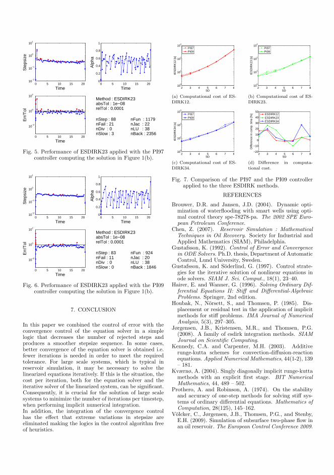
0 5 10 15 2010
−2
10−1
100
101
Time
Ste
psiz
e
0 5 10 15 20
10−2
100
102
Time
Err
/Tol
0 5 10 15 200
0.2
0.4
0.6
0.8
1
TimeA
lpha
Method : ESDIRK23absTol : 1e−08relTol : 0.0001
nStep : 88nFail : 21nDiv : 0nSlow : 3
nFun : 1179nJac : 22nLU : 38nBack : 2356
Fig. 5. Performance of ESDIRK23 applied with the PI97controller computing the solution in Figure 1(b).
0 5 10 15 2010
−2
10−1
100
101
Time
Ste
psiz
e
0 5 10 15 20
10−2
100
102
Time
Err
/Tol
0 5 10 15 200
0.2
0.4
0.6
0.8
1
Time
Alp
ha
Method : ESDIRK23absTol : 1e−08relTol : 0.0001
nStep : 83nFail : 11nDiv : 0nSlow : 0
nFun : 924nJac : 20nLU : 38nBack : 1846
Fig. 6. Performance of ESDIRK23 applied with the PI09controller computing the solution in Figure 1(b).
7. CONCLUSION
In this paper we combined the control of error with theconvergence control of the equation solver in a simplelogic that decreases the number of rejected steps andproduces a smoother stepsize sequence. In some cases,better convergence of the equation solver is obtained i.e.fewer iterations is needed in order to meet the requiredtolerance. For large scale systems, which is typical inreservoir simulation, it may be necessary to solve thelinearized equations iteratively. If this is the situation, thecost per iteration, both for the equation solver and theiterative solver of the linearized system, can be significant.Consequently, it is crucial for the solution of large scalesystems to minimize the number of iterations per timestep,when performing implicit numerical integration.In addition, the integration of the convergence controlhas the effect that extreme variations in stepsize areeliminated making the logics in the control algorithm freeof heuristics.
2 3 4 5 6 7 810
0
101
102
103
SD
tES
DIR
K12
[s]
PI97PI09
(a) Computational cost of ES-DIRK12.
2 3 4 5 6 7 810
0
101
102
103
SD
tES
DIR
K23
[s]
PI97PI09
(b) Computational cost of ES-DIRK23.
2 3 4 5 6 7 810
0
101
102
103
SD
tES
DIR
K34
[s]
PI97PI09
(c) Computational cost of ES-DIRK34.
2 3 4 5 6 7 8−20
−10
0
10
20
30
40
50
SD
Diff
eren
ce in
com
p. ti
me
[%]
ESDIRK12ESDIRK23ESDIRK34
(d) Difference in computa-tional cost.
Fig. 7. Comparison of the PI97 and the PI09 controllerapplied to the three ESDIRK methods.
REFERENCES
Brouwer, D.R. and Jansen, J.D. (2004). Dynamic opti-mization of waterflooding with smart wells using opti-mal control theory spe-78278-pa. The 2002 SPE Euro-pean Petroleum Conference.
Chen, Z. (2007). Reservoir Simulation : MathematicalTechniques in Oil Recovery. Society for Industrial andApplied Mathematics (SIAM), Philadelphia.
Gustafsson, K. (1992). Control of Error and Convergencein ODE Solvers. Ph.D. thesis, Department of AutomaticControl, Lund University, Sweden.
Gustafsson, K. and Soderlind, G. (1997). Control strate-gies for the iterative solution of nonlinear equations inode solvers. SIAM J. Sci. Comput., 18(1), 23–40.
Hairer, E. and Wanner, G. (1996). Solving Ordinary Dif-ferential Equations II: Stiff and Differential-AlgebraicProblems. Springer, 2nd edition.
Houbak, N., Norsett, S., and Thomsen, P. (1985). Dis-placement or residual test in the application of implicitmethods for stiff problems. IMA Journal of NumericalAnalysis, 5(3), 297–305.
Jørgensen, J.B., Kristensen, M.R., and Thomsen, P.G.(2008). A family of esdirk integration methods. SIAMJournal on Scientific Computing.
Kennedy, C.A. and Carpenter, M.H. (2003). Additiverunge-kutta schemes for convection-diffusion-reactionequations. Applied Numerical Mathematics, 44(1-2), 139– 181.
Kværnø, A. (2004). Singly diagonally implicit runge-kuttamethods with an explicit first stage. BIT NumericalMathematics, 44, 489 – 502.
Prothero, A. and Robinson, A. (1974). On the stabilityand accuracy of one-step methods for solving stiff sys-tems of ordinary differential equations. Mathematics ofComputation, 28(125), 145–162.
Volcker, C., Jørgensen, J.B., Thomsen, P.G., and Stenby,E.H. (2009). Simulation of subsurface two-phase flow inan oil reservoir. The European Control Conference 2009.

APPENDIX FPaper C
Explicit Singly Diagonally Implicit Runge-kutta Methodsand Adaptive Stepsize Control for Reservoir Simulation
Authors:
Carsten Völcker, John Bagterp Jørgensen, Per Grove Thomsen andErling Halfdan Stenby
Published in:
Proceedings of 12th European Conference on the Mathematicsof Oil Recovery (ECMOR XII)Oxford, UK6-9 September 2010
147

Explicit Singly Diagonally Implicit Runge-kutta Methods andAdaptive Stepsize Control for Reservoir Simulation
Carsten Volcker∗ John Bagterp Jørgensen∗
Per Grove Thomsen∗ Erling Halfdan Stenby∗∗
∗ Department of Informatics and Mathematical Modeling, Technical University of Denmark,DK-2800 Kgs. Lyngby, Denmark (e-mail: cv,jbj,[email protected])
∗∗ Department of Chemical and Biochemical Engineering, Technical University of Denmark,DK-2800 Kgs. Lyngby, Denmark (e-mail: [email protected])
Abstract
The implicit Euler method, normally refered to as the fully implicit (FIM) method, and theimplicit pressure explicit saturation (IMPES) method are the traditional choices for temporaldiscretization in reservoir simulation. The FIM method offers unconditionally stability in thesense of discrete approximations, while the IMPES scheme benefits from the explicit treatmentof the saturation. However, in tems of controlling the integration error, the low order of theFIM method leads to small integration steps, while the explicit treatment of the saturation mayrestrict the stepsizes for the IMPES scheme. Current reservoir simulators apply timesteppingalgorithms that are based on safeguarded heuristics, and can neither guarantee convergencein the underlying equation solver, nor provide estimates of the relations between convergence,integration error and stepsizes.We establish predictive stepsize control applied to high order methods for temporal discretiza-tion in reservoir simulation. The family of Runge-Kutta methods is presented and in particularthe explicit singly diagonally implicit Runge-Kutta (ESDIRK) method with an embedded errorestimate is described. A predictive stepsize adjustment rule based on error estimates and con-vergence control of the integrated iterative solver is presented. We try to improve the predictivestepsize control through an extended communication between the convergence rate, the errorcontrol and the stepsize.
Keywords: Reservoir simulation, implicit Runge-Kutta methods, ESDIRK, Newton-Raphson,convergence control, error control, stepsize selection.
Introduction
Reservoir simulators are computer programs that solve the equations for heat and mass flow inporous media. Numerical integration is one of the basic steps involved in the simulation process.The number and type of equations to be solved depend on the geological characteristics of thereservoir, the characteristics of the reservoir fluids, and the oil recovery process to be modeled.Choosing the appropriate method of integration involves deciding on factors such as the order ofthe integration scheme, stability properties, and concern on computational efficiency. ESDIRKmethods have been applied successfully for solution of convection-diffusion-reaction problems(Kennedy and Carpenter (2003)). This class of methods is computationally efficient, and bothA- and L-stable stiffly accurate ESDIRK methods of various order, with an embedded methodfor error estimation, have been derived by Kværnø (2004) and Jørgensen et al. (2008). In ad-dition, a robust adaptive stepsize selection is essential to an efficient numerical integration. Anadaptive stepsize selection aims to keep the error estimate bounded i.e. close to a user-specifiedtolerance by adjusting the timestep. The nonlinear residual equations arising in fully implicitmethods has to be solved iteratively. Thus in implicit integration the convergence in the equa-tion solver has to be monitored. Gustafsson (1992) suggested a strategy for stepsize selectionbased on the error estimates provided by embedded Runge-Kutta methods.
ECMOR XII – 12th European Conference on the Mathematics of Oil Recovery6 – 9 September 2010, Oxford, UK
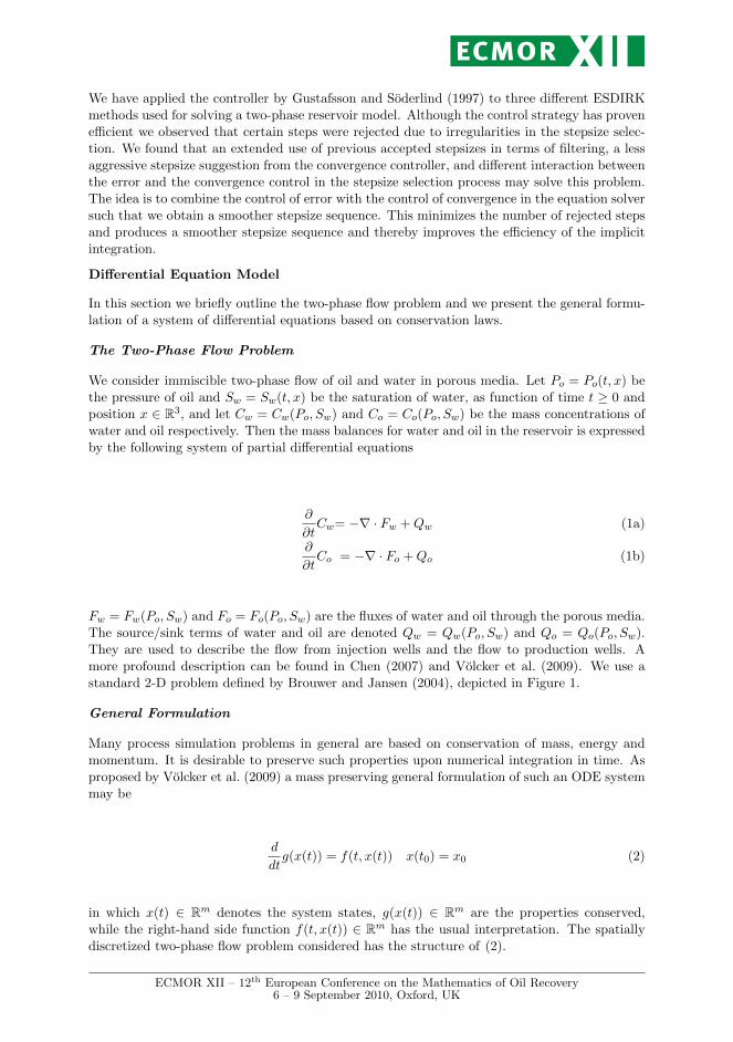
We have applied the controller by Gustafsson and Soderlind (1997) to three different ESDIRKmethods used for solving a two-phase reservoir model. Although the control strategy has provenefficient we observed that certain steps were rejected due to irregularities in the stepsize selec-tion. We found that an extended use of previous accepted stepsizes in terms of filtering, a lessaggressive stepsize suggestion from the convergence controller, and different interaction betweenthe error and the convergence control in the stepsize selection process may solve this problem.The idea is to combine the control of error with the control of convergence in the equation solversuch that we obtain a smoother stepsize sequence. This minimizes the number of rejected stepsand produces a smoother stepsize sequence and thereby improves the efficiency of the implicitintegration.
Differential Equation Model
In this section we briefly outline the two-phase flow problem and we present the general formu-lation of a system of differential equations based on conservation laws.
The Two-Phase Flow Problem
We consider immiscible two-phase flow of oil and water in porous media. Let Po = Po(t, x) bethe pressure of oil and Sw = Sw(t, x) be the saturation of water, as function of time t ≥ 0 andposition x ∈ R3, and let Cw = Cw(Po, Sw) and Co = Co(Po, Sw) be the mass concentrations ofwater and oil respectively. Then the mass balances for water and oil in the reservoir is expressedby the following system of partial differential equations
∂
∂tCw= −∇ · Fw +Qw (1a)
∂
∂tCo = −∇ · Fo +Qo (1b)
Fw = Fw(Po, Sw) and Fo = Fo(Po, Sw) are the fluxes of water and oil through the porous media.The source/sink terms of water and oil are denoted Qw = Qw(Po, Sw) and Qo = Qo(Po, Sw).They are used to describe the flow from injection wells and the flow to production wells. Amore profound description can be found in Chen (2007) and Volcker et al. (2009). We use astandard 2-D problem defined by Brouwer and Jansen (2004), depicted in Figure 1.
General Formulation
Many process simulation problems in general are based on conservation of mass, energy andmomentum. It is desirable to preserve such properties upon numerical integration in time. Asproposed by Volcker et al. (2009) a mass preserving general formulation of such an ODE systemmay be
d
dtg(x(t)) = f(t, x(t)) x(t0) = x0 (2)
in which x(t) ∈ Rm denotes the system states, g(x(t)) ∈ Rm are the properties conserved,while the right-hand side function f(t, x(t)) ∈ Rm has the usual interpretation. The spatiallydiscretized two-phase flow problem considered has the structure of (2).
ECMOR XII – 12th European Conference on the Mathematics of Oil Recovery6 – 9 September 2010, Oxford, UK

x [m]
y [m
]
0 100 200 300 4000
50
100
150
200
250
300
350
400
450
0
2000
4000
6000
8000
10000
12000
(a) Permeability field [mDa].
x [m]
y [m
]
0 100 200 300 4000
50
100
150
200
250
300
350
400
450
0.2
0.3
0.4
0.5
0.6
0.7
(b) Oil saturation, 0.1 PVI.
x [m]
y [m
]
0 100 200 300 4000
50
100
150
200
250
300
350
400
450
0.2
0.3
0.4
0.5
0.6
0.7
(c) Oil saturation, 0.3 PVI.
x [m]
y [m
]
0 100 200 300 4000
50
100
150
200
250
300
350
400
450
0.1
0.2
0.3
0.4
0.5
0.6
(d) Oil saturation, 1 PVI.
Figure 1 Water flooding example, 1 pore volume injected (PVI) over 360 days.
Integration Methods
In this section different classes of Runge-Kutta methods are outlined. In particular ESDIRKmethods are described.
Runge-Kutta Integration
An s-stage Runge-Kutta method for integration of (2) can be expressed as
Ti = tn + hnci i ∈ S1 (3a)
g(Xi) = g(xn) + hn
s∑
j=1
aijf(Tj , Xj) i ∈ S1 (3b)
g(xn+1) = g(xn) + hn
s∑
j=1
bjf(Tj , Xj) (3c)
where Xi are the internal stage values being numerical approximations to x(Ti). xn+1 is thestep computed at tn+1 = tn + hn. The set Si denotes the internal stages i, i + 1, . . . , s. Thes-stage Runge-Kutta method (3) may be denoted in terms of its Butchter tableau
c1 a11 a12 · · · a1sc2 a21 a22 · · · a2s...
......
. . ....
cs as1 as2 · · · assxn+1 b1 b2 · · · bs
(4)
ECMOR XII – 12th European Conference on the Mathematics of Oil Recovery6 – 9 September 2010, Oxford, UK
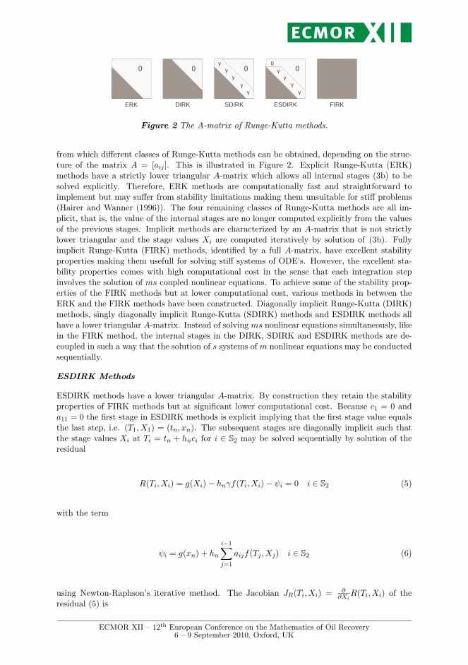
0 0 0 00
γγ
γγ
γγ
γγ
γ
ERK DIRK SDIRK ESDIRK FIRK
Figure 2 The A-matrix of Runge-Kutta methods.
from which different classes of Runge-Kutta methods can be obtained, depending on the struc-ture of the matrix A = [aij ]. This is illustrated in Figure 2. Explicit Runge-Kutta (ERK)methods have a strictly lower triangular A-matrix which allows all internal stages (3b) to besolved explicitly. Therefore, ERK methods are computationally fast and straightforward toimplement but may suffer from stability limitations making them unsuitable for stiff problems(Hairer and Wanner (1996)). The four remaining classes of Runge-Kutta methods are all im-plicit, that is, the value of the internal stages are no longer computed explicitly from the valuesof the previous stages. Implicit methods are characterized by an A-matrix that is not strictlylower triangular and the stage values Xi are computed iteratively by solution of (3b). Fullyimplicit Runge-Kutta (FIRK) methods, identified by a full A-matrix, have excellent stabilityproperties making them usefull for solving stiff systems of ODE’s. However, the excellent sta-bility properties comes with high computational cost in the sense that each integration stepinvolves the solution of ms coupled nonlinear equations. To achieve some of the stability prop-erties of the FIRK methods but at lower computational cost, various methods in between theERK and the FIRK methods have been constructed. Diagonally implicit Runge-Kutta (DIRK)methods, singly diagonally implicit Runge-Kutta (SDIRK) methods and ESDIRK methods allhave a lower triangular A-matrix. Instead of solvingms nonlinear equations simultaneously, likein the FIRK method, the internal stages in the DIRK, SDIRK and ESDIRK methods are de-coupled in such a way that the solution of s systems of m nonlinear equations may be conductedsequentially.
ESDIRK Methods
ESDIRK methods have a lower triangular A-matrix. By construction they retain the stabilityproperties of FIRK methods but at significant lower computational cost. Because c1 = 0 anda11 = 0 the first stage in ESDIRK methods is explicit implying that the first stage value equalsthe last step, i.e. (T1, X1) = (tn, xn). The subsequent stages are diagonally implicit such thatthe stage values Xi at Ti = tn + hnci for i ∈ S2 may be solved sequentially by solution of theresidual
R(Ti, Xi) = g(Xi)− hnγf(Ti, Xi)− ψi = 0 i ∈ S2 (5)
with the term
ψi = g(xn) + hn
i−1∑
j=1
aijf(Tj , Xj) i ∈ S2 (6)
using Newton-Raphson’s iterative method. The Jacobian JR(Ti, Xi) = ∂∂Xi
R(Ti, Xi) of theresidual (5) is
ECMOR XII – 12th European Conference on the Mathematics of Oil Recovery6 – 9 September 2010, Oxford, UK
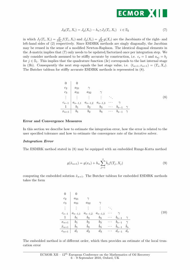
JR(Ti, Xi) = Jg(Xi)− hnγJf (Ti, Xi) i ∈ S2 (7)
in which Jf (Ti, Xi) =∂
∂Xif(Ti, Xi) and Jg(Xi) =
ddXi
g(Xi) are the Jacobiants of the right- andleft-hand sides of (2) respectively. Since ESDIRK methods are singly diagonally, the Jacobianmay be reused in the sense of a modified Newton-Raphson. The identical diagonal elements inthe A-matrix implies that (7) only needs to be updated/factorized once per integration step. Weonly consider methods assumed to be stiffly accurate by construction, i.e. cs = 1 and asj = bjfor j ∈ S1. This implies that the quadrature function (3c) corresponds to the last internal stagein (3b). Consequently the next step equals the last stage value, i.e. (tn+1, xn+1) = (Ts, Xs).The Butcher tableau for stiffly accurate ESDIRK methods is represented in (8).
0 0c2 a21 γc3 a31 a32 γ...
......
.... . .
cs−1 as−1,1 as−1,2 as−1,3 · · · γ1 b1 b2 b3 · · · bs−1 γ
xn+1 b1 b2 b3 · · · bs−1 γ
(8)
Error and Convergence Measures
In this section we describe how to estimate the integration error, how the error is related to theuser specified tolerance and how to estimate the convergence rate of the iterative solver.
Integration Error
The ESDIRK method stated in (8) may be equipped with an embedded Runge-Kutta method
g(xn+1) = g(xn) + hn
s∑
j=1
bjf(Tj , Xj) (9)
computing the embedded solution xn+1. The Butcher tableau for embedded ESDIRK methodstakes the form
0 0c2 a21 γc3 a31 a32 γ...
......
.... . .
cs−1 as−1,1 as−1,2 as−1,3 · · · γ1 b1 b2 b3 · · · bs−1 γ
xn+1 b1 b2 b3 · · · bs−1 γ
xn+1 b1 b2 b3 · · · bs−1 bsen+1 d1 d2 d3 · · · ds−1 ds
(10)
The embedded method is of different order, which then provides an estimate of the local trun-cation error
ECMOR XII – 12th European Conference on the Mathematics of Oil Recovery6 – 9 September 2010, Oxford, UK
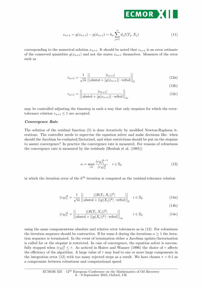
en+1 = g(xn+1)− g(xn+1) = hn
s∑
j=1
djf(Tj , Xj) (11)
corresponding to the numerical solution xn+1. It should be noted that en+1 is an error estimateof the conserved quantities g(xn+1) and not the states xn+1 themselves. Measures of the errorsuch as
rn+1 =1√m
∣∣∣∣∣∣∣∣
|en+1|abstol + |g(xn+1)| · reltol
∣∣∣∣∣∣∣∣2
(12a)
(12b)
rn+1 =
∣∣∣∣∣∣∣∣
|en+1|abstol + |g(xn+1)| · reltol
∣∣∣∣∣∣∣∣∞
(12c)
may be controlled adjusting the timestep in such a way that only stepsizes for which the error-tolerance relation rn+1 ≤ 1 are accepted.
Convergence Rate
The solution of the residual function (5) is done iteratively by modified Newton-Raphson it-erations. The controller needs to supervise the equation solver and make decisions like: whenshould the Jacobian be evaluated/factorized, and what restrictions should be put on the stepsizeto assure convergence? In practice the convergence rate is measured. For reasons of robustnessthe convergence rate is measured by the residuals (Houbak et al. (1985))
α = maxi,k
(rR)k−1i
(rR)kii ∈ S2 (13)
in which the iteration error of the kth iteration is computed as the residual-tolerance relation
(rR)ki =
1√m
∣∣∣∣∣∣∣∣
|(R(Ti, Xi))k|
abstol + |(g(Xi))k| · reltol
∣∣∣∣∣∣∣∣2
i ∈ S2 (14a)
(14b)
(rR)ki =
∣∣∣∣∣∣∣∣
|(R(Ti, Xi))k|
abstol + |(g(Xi))k| · reltol
∣∣∣∣∣∣∣∣∞
i ∈ S2 (14c)
using the same componentwise absolute and relative error tolerances as in (12). For robustnessthe iteration sequence should be contractive. If for some k during the iterations α ≥ 1 the itera-tion sequence is terminated. In the event of termination either a Jacobian update/factorizationis called for or the stepsize is restricted. In case of convergence, the equation solver is success-fully stopped when (rR)
ki ≤ τ . As noticed in Hairer and Wanner (1996) the choice of τ affects
the efficiency of the algorithm. A large value of τ may lead to one or more large components inthe integration error (12) with too many rejected steps as a result. We have chosen τ = 0.1 asa compromise between robustness and computational speed.
ECMOR XII – 12th European Conference on the Mathematics of Oil Recovery6 – 9 September 2010, Oxford, UK
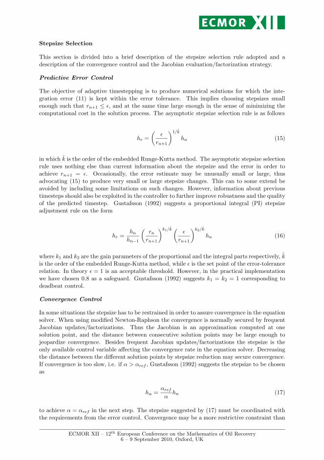
Stepsize Selection
This section is divided into a brief description of the stepsize selection rule adopted and adescription of the convergence control and the Jacobian evaluation/factorization strategy.
Predictive Error Control
The objective of adaptive timestepping is to produce numerical solutions for which the inte-gration error (11) is kept within the error tolerance. This implies choosing stepsizes smallenough such that rn+1 ≤ ε, and at the same time large enough in the sense of minimizing thecomputational cost in the solution process. The asymptotic stepsize selection rule is as follows
hr =
(ε
rn+1
)1/k
hn (15)
in which k is the order of the embedded Runge-Kutta method. The asymptotic stepsize selectionrule uses nothing else than current information about the stepsize and the error in order toachieve rn+1 = ε. Occasionally, the error estimate may be unusually small or large, thusadvocating (15) to produce very small or large stepsize changes. This can to some extend beavoided by including some limitations on such changes. However, information about previoustimesteps should also be exploited in the controller to further improve robustness and the qualityof the predicted timestep. Gustafsson (1992) suggests a proportional integral (PI) stepsizeadjustment rule on the form
hr =hnhn−1
(rnrn+1
)k1/k ( ε
rn+1
)k2/k
hn (16)
where k1 and k2 are the gain parameters of the proportional and the integral parts respectively, kis the order of the embedded Runge-Kutta method, while ε is the set point of the error-tolerancerelation. In theory ε = 1 is an acceptable threshold. However, in the practical implementationwe have chosen 0.8 as a safeguard. Gustafsson (1992) suggests k1 = k2 = 1 corresponding todeadbeat control.
Convergence Control
In some situations the stepsize has to be restrained in order to assure convergence in the equationsolver. When using modified Newton-Raphson the convergence is normally secured by frequentJacobian updates/factorizations. Thus the Jacobian is an approximation computed at onesolution point, and the distance between consecutive solution points may be large enough tojeopardize convergence. Besides frequent Jacobian updates/factorizations the stepsize is theonly available control variable affecting the convergence rate in the equation solver. Decreasingthe distance between the different solution points by stepsize reduction may secure convergence.If convergence is too slow, i.e. if α > αref , Gustafsson (1992) suggests the stepsize to be chosenas
hα =αref
αhn (17)
to achieve α = αref in the next step. The stepsize suggested by (17) must be coordinated withthe requirements from the error control. Convergence may be a more restrictive constraint than
ECMOR XII – 12th European Conference on the Mathematics of Oil Recovery6 – 9 September 2010, Oxford, UK
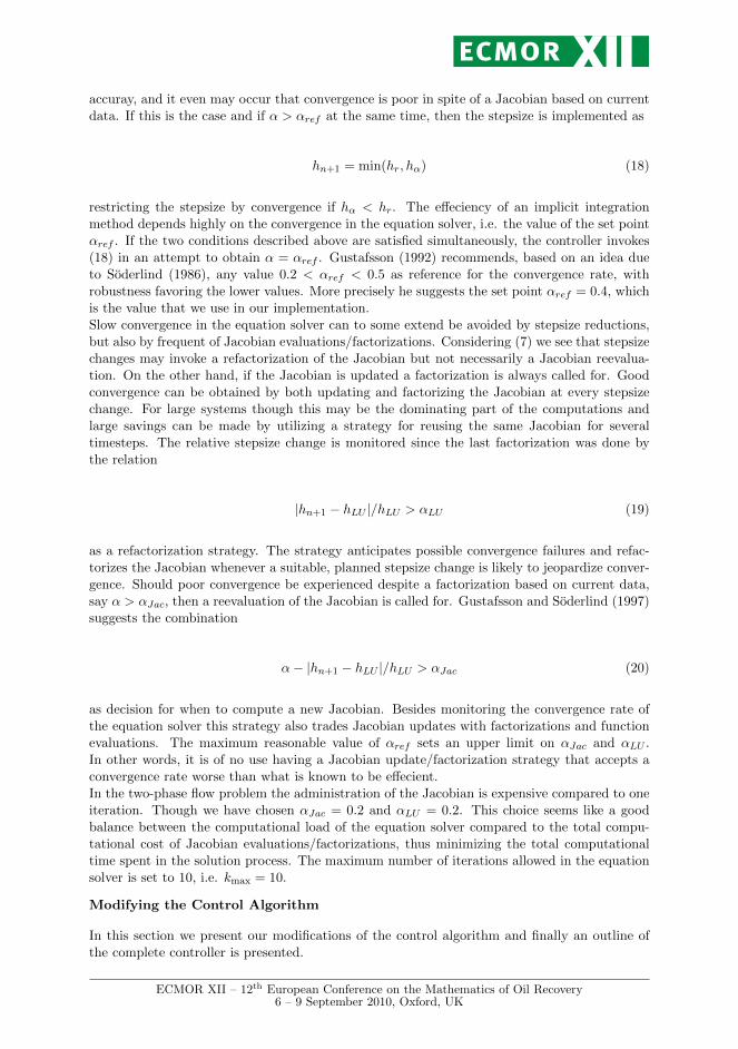
accuray, and it even may occur that convergence is poor in spite of a Jacobian based on currentdata. If this is the case and if α > αref at the same time, then the stepsize is implemented as
hn+1 = min(hr, hα) (18)
restricting the stepsize by convergence if hα < hr. The effeciency of an implicit integrationmethod depends highly on the convergence in the equation solver, i.e. the value of the set pointαref . If the two conditions described above are satisfied simultaneously, the controller invokes(18) in an attempt to obtain α = αref . Gustafsson (1992) recommends, based on an idea dueto Soderlind (1986), any value 0.2 < αref < 0.5 as reference for the convergence rate, withrobustness favoring the lower values. More precisely he suggests the set point αref = 0.4, whichis the value that we use in our implementation.Slow convergence in the equation solver can to some extend be avoided by stepsize reductions,but also by frequent of Jacobian evaluations/factorizations. Considering (7) we see that stepsizechanges may invoke a refactorization of the Jacobian but not necessarily a Jacobian reevalua-tion. On the other hand, if the Jacobian is updated a factorization is always called for. Goodconvergence can be obtained by both updating and factorizing the Jacobian at every stepsizechange. For large systems though this may be the dominating part of the computations andlarge savings can be made by utilizing a strategy for reusing the same Jacobian for severaltimesteps. The relative stepsize change is monitored since the last factorization was done bythe relation
|hn+1 − hLU |/hLU > αLU (19)
as a refactorization strategy. The strategy anticipates possible convergence failures and refac-torizes the Jacobian whenever a suitable, planned stepsize change is likely to jeopardize conver-gence. Should poor convergence be experienced despite a factorization based on current data,say α > αJac, then a reevaluation of the Jacobian is called for. Gustafsson and Soderlind (1997)suggests the combination
α− |hn+1 − hLU |/hLU > αJac (20)
as decision for when to compute a new Jacobian. Besides monitoring the convergence rate ofthe equation solver this strategy also trades Jacobian updates with factorizations and functionevaluations. The maximum reasonable value of αref sets an upper limit on αJac and αLU .In other words, it is of no use having a Jacobian update/factorization strategy that accepts aconvergence rate worse than what is known to be effecient.In the two-phase flow problem the administration of the Jacobian is expensive compared to oneiteration. Though we have chosen αJac = 0.2 and αLU = 0.2. This choice seems like a goodbalance between the computational load of the equation solver compared to the total compu-tational cost of Jacobian evaluations/factorizations, thus minimizing the total computationaltime spent in the solution process. The maximum number of iterations allowed in the equationsolver is set to 10, i.e. kmax = 10.
Modifying the Control Algorithm
In this section we present our modifications of the control algorithm and finally an outline ofthe complete controller is presented.
ECMOR XII – 12th European Conference on the Mathematics of Oil Recovery6 – 9 September 2010, Oxford, UK
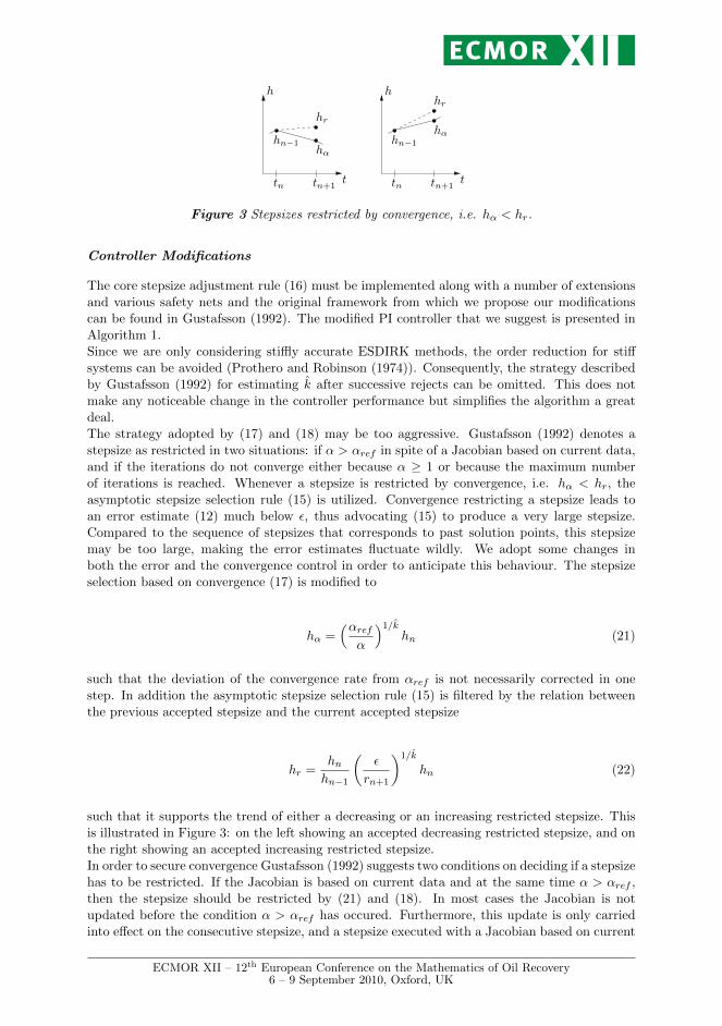
tttn+1
h h
tn+1tn tn
hn−1hα
hn−1
hαhr
hr
Figure 3 Stepsizes restricted by convergence, i.e. hα < hr.
Controller Modifications
The core stepsize adjustment rule (16) must be implemented along with a number of extensionsand various safety nets and the original framework from which we propose our modificationscan be found in Gustafsson (1992). The modified PI controller that we suggest is presented inAlgorithm 1.Since we are only considering stiffly accurate ESDIRK methods, the order reduction for stiffsystems can be avoided (Prothero and Robinson (1974)). Consequently, the strategy describedby Gustafsson (1992) for estimating k after successive rejects can be omitted. This does notmake any noticeable change in the controller performance but simplifies the algorithm a greatdeal.The strategy adopted by (17) and (18) may be too aggressive. Gustafsson (1992) denotes astepsize as restricted in two situations: if α > αref in spite of a Jacobian based on current data,and if the iterations do not converge either because α ≥ 1 or because the maximum numberof iterations is reached. Whenever a stepsize is restricted by convergence, i.e. hα < hr, theasymptotic stepsize selection rule (15) is utilized. Convergence restricting a stepsize leads toan error estimate (12) much below ε, thus advocating (15) to produce a very large stepsize.Compared to the sequence of stepsizes that corresponds to past solution points, this stepsizemay be too large, making the error estimates fluctuate wildly. We adopt some changes inboth the error and the convergence control in order to anticipate this behaviour. The stepsizeselection based on convergence (17) is modified to
hα =(αref
α
)1/khn (21)
such that the deviation of the convergence rate from αref is not necessarily corrected in onestep. In addition the asymptotic stepsize selection rule (15) is filtered by the relation betweenthe previous accepted stepsize and the current accepted stepsize
hr =hnhn−1
(ε
rn+1
)1/k
hn (22)
such that it supports the trend of either a decreasing or an increasing restricted stepsize. Thisis illustrated in Figure 3: on the left showing an accepted decreasing restricted stepsize, and onthe right showing an accepted increasing restricted stepsize.In order to secure convergence Gustafsson (1992) suggests two conditions on deciding if a stepsizehas to be restricted. If the Jacobian is based on current data and at the same time α > αref ,then the stepsize should be restricted by (21) and (18). In most cases the Jacobian is notupdated before the condition α > αref has occured. Furthermore, this update is only carriedinto effect on the consecutive stepsize, and a stepsize executed with a Jacobian based on current
ECMOR XII – 12th European Conference on the Mathematics of Oil Recovery6 – 9 September 2010, Oxford, UK
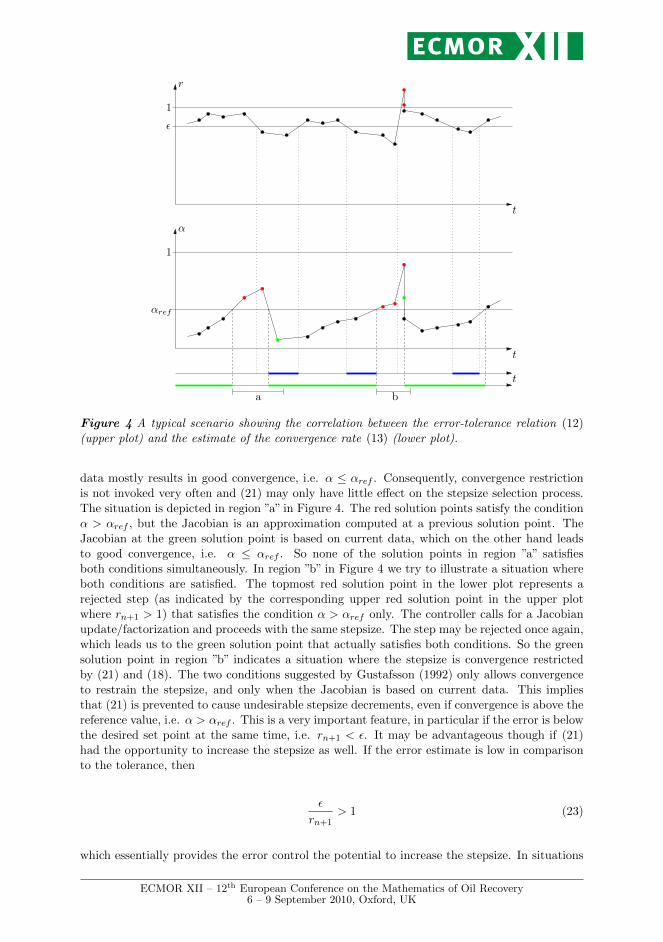
1
1
t
t
t
r
α
ε
ba
αref
Figure 4 A typical scenario showing the correlation between the error-tolerance relation (12)(upper plot) and the estimate of the convergence rate (13) (lower plot).
data mostly results in good convergence, i.e. α ≤ αref . Consequently, convergence restrictionis not invoked very often and (21) may only have little effect on the stepsize selection process.The situation is depicted in region ”a” in Figure 4. The red solution points satisfy the conditionα > αref , but the Jacobian is an approximation computed at a previous solution point. TheJacobian at the green solution point is based on current data, which on the other hand leadsto good convergence, i.e. α ≤ αref . So none of the solution points in region ”a” satisfiesboth conditions simultaneously. In region ”b” in Figure 4 we try to illustrate a situation whereboth conditions are satisfied. The topmost red solution point in the lower plot represents arejected step (as indicated by the corresponding upper red solution point in the upper plotwhere rn+1 > 1) that satisfies the condition α > αref only. The controller calls for a Jacobianupdate/factorization and proceeds with the same stepsize. The step may be rejected once again,which leads us to the green solution point that actually satisfies both conditions. So the greensolution point in region ”b” indicates a situation where the stepsize is convergence restrictedby (21) and (18). The two conditions suggested by Gustafsson (1992) only allows convergenceto restrain the stepsize, and only when the Jacobian is based on current data. This impliesthat (21) is prevented to cause undesirable stepsize decrements, even if convergence is above thereference value, i.e. α > αref . This is a very important feature, in particular if the error is belowthe desired set point at the same time, i.e. rn+1 < ε. It may be advantageous though if (21)had the opportunity to increase the stepsize as well. If the error estimate is low in comparisonto the tolerance, then
ε
rn+1> 1 (23)
which essentially provides the error control the potential to increase the stepsize. In situations
ECMOR XII – 12th European Conference on the Mathematics of Oil Recovery6 – 9 September 2010, Oxford, UK
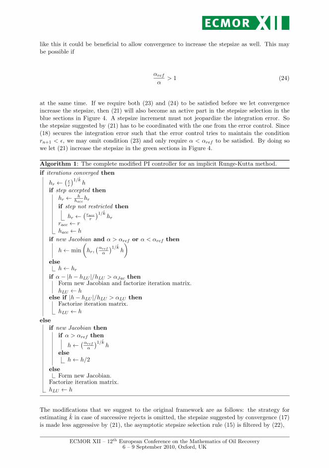
like this it could be beneficial to allow convergence to increase the stepsize as well. This maybe possible if
αref
α> 1 (24)
at the same time. If we require both (23) and (24) to be satisfied before we let convergenceincrease the stepsize, then (21) will also become an active part in the stepsize selection in theblue sections in Figure 4. A stepsize increment must not jeopardize the integration error. Sothe stepsize suggested by (21) has to be coordinated with the one from the error control. Since(18) secures the integration error such that the error control tries to maintain the conditionrn+1 < ε, we may omit condition (23) and only require α < αref to be satisfied. By doing sowe let (21) increase the stepsize in the green sections in Figure 4.
Algorithm 1: The complete modified PI controller for an implicit Runge-Kutta method.
if iterations converged then
hr ←(εr
)1/kh
if step accepted then
hr ← hhacc
hrif step not restricted then
hr ←(raccr
)1/khr
racc ← rhacc ← h
if new Jacobian and α > αref or α < αref then
h← min
(hr,(αref
α
)1/kh
)
elseh← hr
if α− |h− hLU |/hLU > αJac thenForm new Jacobian and factorize iteration matrix.hLU ← h
else if |h− hLU |/hLU > αLU thenFactorize iteration matrix.hLU ← h
elseif new Jacobian then
if α > αref then
h←(αref
α
)1/kh
elseh← h/2
elseForm new Jacobian.
Factorize iteration matrix.hLU ← h
The modifications that we suggest to the original framework are as follows: the strategy forestimating k in case of successive rejects is omitted, the stepsize suggested by convergence (17)is made less aggressive by (21), the asymptotic stepsize selection rule (15) is filtered by (22),
ECMOR XII – 12th European Conference on the Mathematics of Oil Recovery6 – 9 September 2010, Oxford, UK
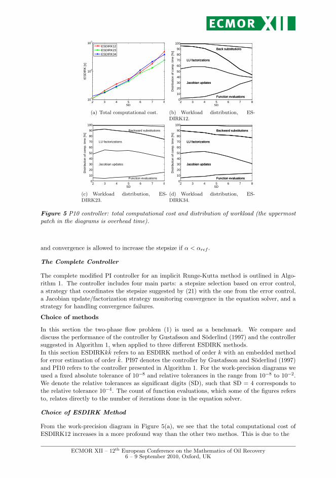
2 3 4 5 6 7 810
1
102
103
SD
tES
DIR
K [s
]
ESDIRK12ESDIRK23ESDIRK34
(a) Total computational cost.
2 3 4 5 6 7 80
10
20
30
40
50
60
70
80
90
100
SD
Dis
trib
utio
n of
com
p. ti
me
[%]
Function evaluations
Jacobian updates
LU factorizations
Back substitutions
Function evaluations
Jacobian updates
LU factorizations
Back substitutions
(b) Workload distribution, ES-DIRK12.
2 3 4 5 6 7 80
10
20
30
40
50
60
70
80
90
100
SD
Dis
trib
utio
n of
com
p. ti
me
[%]
Function evaluations
Jacobian updates
LU factorizations
Backward substitutions
(c) Workload distribution, ES-DIRK23.
2 3 4 5 6 7 80
10
20
30
40
50
60
70
80
90
100
SD
Dis
trib
utio
n of
com
p. ti
me
[%]
Function evaluations
Jacobian updates
LU factorizations
Backward substitutions
Function evaluations
Jacobian updates
LU factorizations
Backward substitutions
(d) Workload distribution, ES-DIRK34.
Figure 5 P10 controller: total computational cost and distribution of workload (the uppermostpatch in the diagrams is overhead time).
and convergence is allowed to increase the stepsize if α < αref .
The Complete Controller
The complete modified PI controller for an implicit Runge-Kutta method is outlined in Algo-rithm 1. The controller includes four main parts: a stepsize selection based on error control,a strategy that coordinates the stepsize suggested by (21) with the one from the error control,a Jacobian update/factorization strategy monitoring convergence in the equation solver, and astrategy for handling convergence failures.
Choice of methods
In this section the two-phase flow problem (1) is used as a benchmark. We compare anddiscuss the performance of the controller by Gustafsson and Soderlind (1997) and the controllersuggested in Algorithm 1, when applied to three different ESDIRK methods.In this section ESDIRKkk refers to an ESDIRK method of order k with an embedded methodfor error estimation of order k. PI97 denotes the controller by Gustafsson and Soderlind (1997)and PI10 refers to the controller presented in Algorithm 1. For the work-precision diagrams weused a fixed absolute tolerance of 10−8 and relative tolerances in the range from 10−8 to 10−2.We denote the relative tolerances as significant digits (SD), such that SD = 4 corresponds tothe relative tolerance 10−4. The count of function evaluations, which some of the figures refersto, relates directly to the number of iterations done in the equation solver.
Choice of ESDIRK Method
From the work-precision diagram in Figure 5(a), we see that the total computational cost ofESDIRK12 increases in a more profound way than the other two methos. This is due to the
ECMOR XII – 12th European Conference on the Mathematics of Oil Recovery6 – 9 September 2010, Oxford, UK
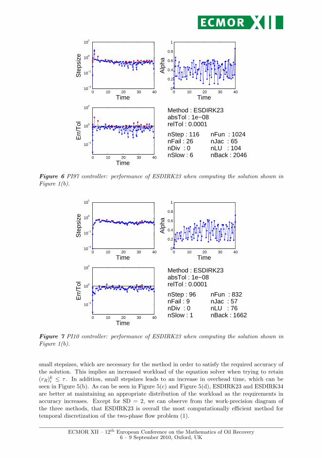
0 10 20 30 4010
−2
10−1
100
101
Time
Ste
psiz
e
0 10 20 30 40
10−2
100
102
Time
Err
/Tol
0 10 20 30 400
0.2
0.4
0.6
0.8
1
Time
Alp
ha
Method : ESDIRK23absTol : 1e−08relTol : 0.0001
nStep : 116nFail : 26nDiv : 0nSlow : 6
nFun : 1024nJac : 65nLU : 104nBack : 2046
Figure 6 PI97 controller: performance of ESDIRK23 when computing the solution shown inFigure 1(b).
0 10 20 30 4010
−2
10−1
100
101
Time
Ste
psiz
e
0 10 20 30 40
10−2
100
102
Time
Err
/Tol
0 10 20 30 400
0.2
0.4
0.6
0.8
1
Time
Alp
ha
Method : ESDIRK23absTol : 1e−08relTol : 0.0001
nStep : 96nFail : 9nDiv : 0nSlow : 1
nFun : 832nJac : 57nLU : 76nBack : 1662
Figure 7 PI10 controller: performance of ESDIRK23 when computing the solution shown inFigure 1(b).
small stepsizes, which are necessary for the method in order to satisfy the required accuracy ofthe solution. This implies an increased workload of the equation solver when trying to retain(rR)
ki ≤ τ . In addition, small stepsizes leads to an increase in overhead time, which can be
seen in Figure 5(b). As can be seen in Figure 5(c) and Figure 5(d), ESDIRK23 and ESDIRK34are better at maintaining an appropriate distribution of the workload as the requirements inaccuracy increases. Except for SD = 2, we can observe from the work-precision diagram ofthe three methods, that ESDIRK23 is overall the most computationally efficient method fortemporal discretization of the two-phase flow problem (1).
ECMOR XII – 12th European Conference on the Mathematics of Oil Recovery6 – 9 September 2010, Oxford, UK

2 3 4 5 6 7 810
1
102
103
SD
tES
DIR
K12
[s]
PI97PI10
(a) Totsl computational cost, ES-DIRK12.
2 3 4 5 6 7 810
1
102
103
SD
tES
DIR
K23
[s]
PI97PI10
(b) Computational cost of ES-DIRK23.
2 3 4 5 6 7 810
1
102
103
SD
tES
DIR
K34
[s]
PI97PI10
(c) Computational cost of ES-DIRK34.
2 3 4 5 6 7 80.8
0.9
1
1.1
1.2
1.3
SD
Rel
ativ
e sp
eedu
p
ESDIRK12ESDIRK23ESDIRK34
(d) Relative speedup, tPI10tPI97
.
Figure 8 Comparison of the PI97 and the PI10 controller applied to the three ESDIRK methods.
Choice of Controller
The stepsize sequences for the PI97 and the PI10 controllers are depicted in Figure 6 and inFigure 7 respectively. It must be mentioned that nStep, nFail and nSlow refers to the number oftimesteps used in order to obtain the solution, the number of steps rejected by the error control,i.e. rn+1 > 1, and the amount of steps rejected because the maximum number of iterationsis reached. By comparing the performance of the two controllers, we see that fewer Jacobianevaluations/factorizations is required by the PI10 controller in the sense of maintaining goodconvergence in the equation solver. Thus fewer iterations is necessary in order to complete theintegration. Because of the less aggressive stepsize change suggested by (21) in connection withthe filtering of the asymptotic stepsize selection rule, a smoother stepsize sequence is obtained bythe PI10 controller. This implies that the PI10 controller provides a solution with lesser rejectedsteps when compared to the performance of the PI97 controller. In Figure 6 several solutionpoints for which rn+1 ε ca be observed. For the same solution points the correspondingstepsizes are small. Due to the ability of (21) to increase the stepsize as well, this behaviouris only to a lesser extend observed in Figure 7. Hence the PI10 controller may produce largerstepsizes in situations where the integration error and the convergence rate are below theirrespective set points. In Figure 8 we compare the computational cost of the two controllers.We notice, that in comparison to the PI97 controller, a better performance is obtained in therange from 2 to 5 SD’s for the PI10 controller. Since high accuracy is not required in reservoirsimulation, we suggest the application of the stepsize controller presented in Algorithm 1 forimplicit integration of dynamical systems like the two-phase flow problem.
Conclusion
We have established a predictive stepsize control applied to high order methods for temporaldiscretization of the two-phase flow problem. The family of Runge-Kutta methods has been
ECMOR XII – 12th European Conference on the Mathematics of Oil Recovery6 – 9 September 2010, Oxford, UK
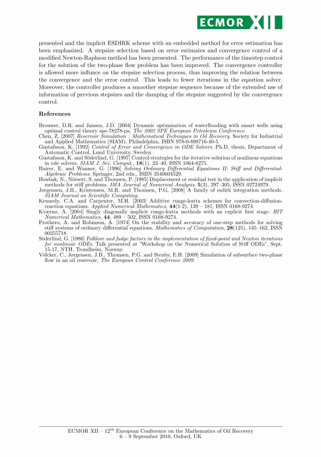
presented and the implicit ESDIRK scheme with an embedded method for error estimation hasbeen emphasized. A stepsize selection based on error estimates and convergence control of amodified Newton-Raphson method has been presented. The performance of the timestep controlfor the solution of the two-phase flow problem has been improved. The convergence controlleris allowed more influnce on the stepsize selection process, thus improving the relation betweenthe convergence and the error control. This leads to fewer iterations in the eqaution solver.Moreover, the controller produces a smoother stepsize sequence because of the extended use ofinformation of previous stepsizes and the damping of the stepsize suggested by the convergencecontrol.
References
Brouwer, D.R. and Jansen, J.D. [2004] Dynamic optimization of waterflooding with smart wells usingoptimal control theory spe-78278-pa. The 2002 SPE European Petroleum Conference.
Chen, Z. [2007] Reservoir Simulation : Mathematical Techniques in Oil Recovery. Society for Industrialand Applied Mathematics (SIAM), Philadelphia, ISBN 978-0-898716-40-5.
Gustafsson, K. [1992] Control of Error and Convergence in ODE Solvers. Ph.D. thesis, Department ofAutomatic Control, Lund University, Sweden.
Gustafsson, K. and Soderlind, G. [1997] Control strategies for the iterative solution of nonlinear equationsin ode solvers. SIAM J. Sci. Comput., 18(1), 23–40, ISSN 1064-8275.
Hairer, E. and Wanner, G. [1996] Solving Ordinary Differential Equations II: Stiff and Differential-Algebraic Problems. Springer, 2nd edn., ISBN 3540604529.
Houbak, N., Norsett, S. and Thomsen, P. [1985] Displacement or residual test in the application of implicitmethods for stiff problems. IMA Journal of Numerical Analysis, 5(3), 297–305, ISSN 02724979.
Jørgensen, J.B., Kristensen, M.R. and Thomsen, P.G. [2008] A family of esdirk integration methods.SIAM Journal on Scientific Computing.
Kennedy, C.A. and Carpenter, M.H. [2003] Additive runge-kutta schemes for convection-diffusion-reaction equations. Applied Numerical Mathematics, 44(1-2), 139 – 181, ISSN 0168-9274.
Kværnø, A. [2004] Singly diagonally implicit runge-kutta methods with an explicit first stage. BITNumerical Mathematics, 44, 489 – 502, ISSN 0168-9274.
Prothero, A. and Robinson, A. [1974] On the stability and accuracy of one-step methods for solvingstiff systems of ordinary differential equations. Mathematics of Computation, 28(125), 145–162, ISSN00255718.
Soderlind, G. [1986] Folklore and fudge factors in the implementation of fixed-point and Newton iterationsfor nonlinear ODEs. Talk presented at ”Workshop on the Numerical Solution of Stiff ODEs”, Sept.15-17, NTH, Trondheim, Norway.
Volcker, C., Jørgensen, J.B., Thomsen, P.G. and Stenby, E.H. [2009] Simulation of subsurface two-phaseflow in an oil reservoir. The European Control Conference 2009.
ECMOR XII – 12th European Conference on the Mathematics of Oil Recovery6 – 9 September 2010, Oxford, UK
APPENDIX GPaper D
NMPC for Oil Reservoir Production Optimization
Authors:
Carsten Völcker, John Bagterp Jørgensen, Per Grove Thomsen andErling Halfdan Stenby
Published in:
Proceedings of 21st European Symposium on Computer-AidedProcess Engineering (ESCAPE21)Chalkidiki, Greece29 May - 1 June 2011
163
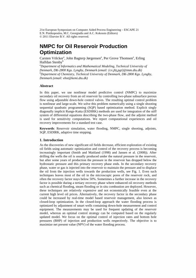
21st European Symposium on Computer Aided Process Engineering – ESCAPE 21 E.N. Pistikopoulos, M.C. Georgiadis and A.C. Kokossis (Editors) © 2011 Elsevier B.V. All rights reserved.
NMPC for Oil Reservoir Production Optimization Carsten Völckera, John Bagterp Jørgensena, Per Grove Thomsena, Erling Halfdan Stenbyb
aDepartment of Informatics and Mathematical Modeling, Technical University of Denmark, DK-2800 Kgs. Lyngby, Denmark (email: cv,jbj,[email protected])
bDepartment of Chemistry, Technical University of Denmark, DK-2800 Kgs. Lyngby, Denmark (email: [email protected])
Abstract
In this paper, we use nonlinear model predictive control (NMPC) to maximize secondary oil recovery from an oil reservoir by controlling two-phase subsurface porous flow using adjustable down-hole control valves. The resulting optimal control problem is nonlinear and large-scale. We solve this problem numerically using a single shooting sequential quadratic programming (SQP) based optimization method. Explicit singly diagonally implicit Runge-Kutta (ESDIRK) methods are used for integration of the stiff system of differential equations describing the two-phase flow, and the adjoint method is used for sensitivity computations. We report computational experiences and oil recovery improvements for a standard test case.
Keywords: Reservoir simulation, water flooding, NMPC, single shooting, adjoints, SQP, ESDIRK, adaptive time stepping.
1. Introduction As the discoveries of new significant oil fields decrease, efficient exploration of existing oil fields using automatic optimization and control of the recovery process is becoming increasingly important (Smith and Maitland (1998) and Jansen et al. (2008)). After drilling the wells the oil is usually produced under the natural pressure in the reservoir, but after some years of production the pressure in the reservoir has dropped below the hydrostatic pressure and this primary recovery phase ends. In the secondary recovery phase, water or gas is injected into the reservoir to maintain the pressure and to displace the oil from the injection wells towards the production wells, see Fig. 1. Even such techniques leaves most of the oil in the microscopic pores of the reservoir rock, and often the recovery factor stays below 50%. Sometimes a further increase in the recovery factor is possible during a tertiary recovery phase where enhanced oil recovery methods such as chemical flooding, steam flooding or in situ combustion are deployed. However, these techniques are relatively expensive and not economically feasible even at the current high level oil prices. Alternatively, the recovery factor in the secondary phase could be increased by real-time model based reservoir management, also known as closed-loop optimization. In the closed-loop approach the water flooding process is optimized by adjustment of smart wells containing down-hole measurement and control equipment. The measurements may be used for frequent updating of the reservoir model, whereas an optimal control strategy can be computed based on the regularly updated model. We focus on the optimal control of injection rates and bottom hole pressures (BHP) of injection and production wells respectively. The objective is to maximize net present value (NPV) of the water flooding process.
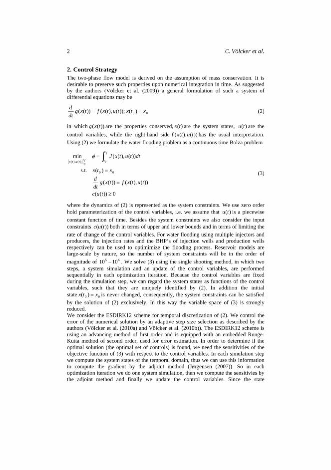
2 C. Völcker et al.
2. Control Strategy The two-phase flow model is derived on the assumption of mass conservation. It is desirable to preserve such properties upon numerical integration in time. As suggested by the authors (Völcker et al. (2009)) a general formulation of such a system of differential equations may be
00 )());(),(())(( xtxtutxftxgdt
d (2)
in which are the properties conserved, are the system states, are the
control variables, while the right-hand side has the usual interpretation.
Using (2) we formulate the water flooding problem as a continuous time Bolza problem
))(( txg )(tx
),(( txf
)(tu
))(tu
0))((
))(),(())((
)(s.t.
))(),((min
00
)(),( 00
tuc
tutxftxgdt
d
xtx
dttutxJf
ftt
t
ttutx
(3)
where the dynamics of (2) is represented as the system constraints. We use zero order hold parameterization of the control variables, i.e. we assume that is a piecewise
constant function of time. Besides the system constraints we also consider the input constraints both in terms of upper and lower bounds and in terms of limiting the
rate of change of the control variables. For water flooding using multiple injectors and producers, the injection rates and the BHP’s of injection wells and production wells respectively can be used to optimimize the flooding process. Reservoir models are large-scale by nature, so the number of system constraints will be in the order of
magnitude of . We solve (3) using the single shooting method, in which two steps, a system simulation and an update of the control variables, are performed sequentially in each optimization iteration. Because the control variables are fixed during the simulation step, we can regard the system states as functions of the control variables, such that they are uniquely identified by (2). In addition the initial state is never changed, consequently, the system constraints can be satisfied
by the solution of (2) exclusively. In this way the variable space of (3) is strongly reduced.
)(tu
))(( tuc
510
0x
610
0 )(tx
We consider the ESDIRK12 scheme for temporal discretization of (2). We control the error of the numerical solution by an adaptive step size selection as described by the authors (Völcker et al. (2010a) and Völcker et al. (2010b)). The ESDIRK12 scheme is using an advancing method of first order and is equipped with an embedded Runge-Kutta method of second order, used for error estimation. In order to determine if the optimal solution (the optimal set of controls) is found, we need the sensitivities of the objective function of (3) with respect to the control variables. In each simulation step we compute the system states of the temporal domain, thus we can use this information to compute the gradient by the adjoint method (Jørgensen (2007)). So in each optimization iteration we do one system simulation, then we compute the sensitivies by the adjoint method and finally we update the control variables. Since the state
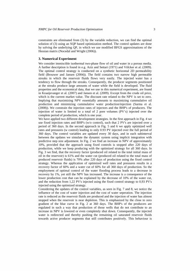
NMPC for Oil Reservoir Production Optimization 3
constraints are eliminated from (3) by the variable reduction, we can find the optimal solution of (3) using an SQP based optimization method. The control updates are done by solving the underlying QP, in which we use modified BFGS approximations of the Hessian matrix (Nocedal and Wright (2006)).
3. Numerical Experiment We consider immiscible isothermal two-phase flow of oil and water in a porous media. A further description is found in e.g. Aziz and Settari (1971) and Völcker et al. (2009). The optimal control strategy is conducted on a synthetic horizontal 2D permeability field (Brouwer and Jansen (2004)). The field contains two narrow high permeable streaks in which the reservoir fluids flows very easily. The injected water has a tendency to flow through the streaks. Consequently, the producer segments positioned at the streaks produce large amounts of water while the field is developed. The fluid properties and the economical data, that we use in this numerical experiment, are found in Kraaijevanger et al. (2007) and Jansen et al. (2009). Except from the crude oil price, which is the current market value. The discount rate related to the NPV is set to zero. Implying that maximizing NPV essentially amounts to maximizing cummulative oil production and minimizing cummulative water production/injection (Sarma et al. (2008)). We constrain the injection rates of injectors and the BHP's of producers. The injection of water is limited to a total of 2 pore volumes (PV’s) injected over the complete period of production, which is one year. We have applied two different development strategies. In the first approach in Fig. 4 we use fixed injection rates and BHP's (w/o control), such that 2 PV's are injected over a period of 360 days. In the second approach in Fig. 5 and 6 we apply optimized well rates and pressures (w control) leading to only 0.93 PV injected over the full period of 360 days. The control variables are updated every 30 days, and in each subinterval between the updates we simulate the dynamic system using implicit integration with predictive step size adjustment. In Fig. 2 we find an increase in NPV of approximately 10%, provided that the approach using fixed controls is stopped after 220 days of production, while we keep producing with the optimized strategy for all 360 days. In Fig. 3 we find, that the recovery factor (produced oil related to the total initial mass of oil in the reservoir) is 61% and the water cut (produced oil related to the total mass of produced reservoir fluids) is 70% after 220 days of production using the fixed control strategy. Whereas the application of optimized well rates and pressures results in a recovery factor of 60% and a water cut of 60% for all 360 days of production. So the employment of optimal control of the water flooding process leads to a decrease in recovery by 1%, yet still the NPV has increased. The increase is a consequence of the lower production cost that can be explained by the decrease of 10% of the water cut, and the reduction from 1,22 PV's injected using the fixed control strategy to 0,93 PV's injected using the optimized strategy. Considering the updates of the control variables, as seen in Fig. 7 and 8, we notice the influence of the cost of water injection and the cost of water seperation. The injection rate is reduced as the reservoir fluids are produced and the injection of water has almost stopped when the reservoir is near depletion. This is emphasized by the close to zero gradient of the blue curve in Fig. 2 at 360 days. The BHP's of the producers are regulated in such a way that production of those wells that do not contribute to an increase in NPV is lowered or even completely shut down. Consequently, the injected water is redirected and thereby pushing the remaining oil saturated reservoir fluids towards active producer segments that still contributes positively. This behaviour is
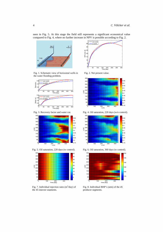
4 C. Völcker et al.
seen in Fig. 5. At this stage the field still represents a significant economical value compared to Fig. 4, where no further increase in NPV is possible according to Fig. 2.
x [m]
y [m
]
0 100 200 300 4000
50
100
150
200
250
300
350
400
450
0.15
0.2
0.25
0.3
0.35
0.4
0.45
0.5
0.55
0.6
0.65
0 50 100 150 200 250 300 3500
0.2
0.4
0.6
Time [day]
Rec
over
y
w/o contrw contr
0 50 100 150 200 250 300 3500
0.2
0.4
0.6
0.8
Time [day]
Wat
er c
ut
w/o contrw contr
Fig. 3. Recovery factor and water cut.
Fig. 1. Schematic view of horizontal wells in the water flooding problem.
0 50 100 150 200 250 300 3500
5
10
15
20
25
30
35
Time [day]
NP
V [m
ill. $
]
w/o contrw contr
Fig. 2. Net present value.
Fig. 4. Oil saturation, 220 days (w/o control).
x [m]
y [m
]
0 100 200 300 4000
50
100
150
200
250
300
350
400
450
0.15
0.2
0.25
0.3
0.35
0.4
0.45
0.5
0.55
0.6
0.65
x [m]
y [m
]
0 100 200 300 4000
50
100
150
200
250
300
350
400
450
0.15
0.2
0.25
0.3
0.35
0.4
0.45
0.5
0.55
0.6
0.65
Fig. 5. Oil saturation, 220 days (w control). Fig. 6. Oil saturation, 360 days (w control).
Time [day]
y [m
]
0 100 200 3000
50
100
150
200
250
300
350
400
450
5
10
15
20
25
30
35
40
45
Time [day]
y [m
]
0 100 200 3000
50
100
150
200
250
300
350
400
450
175
180
185
190
195
200
Fig. 8. Individual BHP’s (atm) of the 45 producer segments.
Fig. 7. Individual injection rates (m3/day) of the 45 injector segments.
NMPC for Oil Reservoir Production Optimization 5
4. Conclusion In this paper, we applied a single shooting SQP based optimization method for production optimization of an oil reservoir. We use a fully implicit integration scheme equipped with an adpative step size control for efficient integration of the model equations, and we compute the sensitivities by the adjoint method. We demonstrate the method on a simple water flooding problem using linear input constraints and low frequency updates of the control variables. The numerical results show an increase of the economical value. A further increase of the economical value of existing oil fields demonstrates the potential of model based optimization as a good alternative to finding new ones.
5. References Aziz, K. and Settari, A. (1971). Petroleum Reservoir Simulation. Applied Science Publishers Ltd,
London, first edition. Brouwer, D.R. and Jansen, J.-D. (2004). Dynamic optimization of waterflooding with smart wells
using optimal control theory. SPE Journal, 9(4), 391-402. Jansen, J.-D., Bosgra, O.H. and Van den Hof, P.M. (2008). Model-Based Control of Multiphase
Flow in Subsurface Oil Reservoirs. Journal of Process Control, 18, 2008, 846-855. Jansen, J.-D., Brouwer, R. and Douma, S.G. (2009). Closed Loop Reservoir Management. SPE
Reservoir Simulation Symposium, Society of Petroleum Engineers, The Woodlands, Texas, 2009.
Jørgensen, J.B. (2007). Adjoint Sensitivity Results for Predictive Control, State- and Parameter-Estimation with Nonlinear Models. Proceedings of the European Control Conference 2007, Kos, Greece, July 2-5, 2007, 3649-3656.
Kraaijevanger, J.F.B.M., Egberts, P.J., Valstar, J.R. and Buurman, H.W. (2007). Optimal Waterflood Design Using the Adjoint Method. SPE Reservoir Simulation Symposium, Society of Petroleum Engineers, Houston, Texas, USA, 2007.
Nocedal, J. and Wright, S.J. (2006). Numerical Optimization. Springer Series in Operations Research and Financial Engineering, New York, USA, 2006, second edition.
Sarma, P., Chen, W.H., Durlofsky, L.J. and Aziz, K. (2008). Production Optimization with Adjoint Models under Nonlinear Control-State Path Inequality Constraints. SPE Evaluation & Engineering, 11(2), 2008, 326-339.
Smith, R.G. and Maitland, G. (1998). The Road Ahead to Real-Time Oil and Gas Reservoir Management. Trans IchemE, 76, 1998, 539-552.
Völcker C., Jørgensen J.B., Thomsen, P.G. and Stenby E.H. (2009). Simulation of subsurface two-phase flow in an oil reservoir. Proceedings of the European Control Conference 2009, Budapest, Hungary, August 23-26, 2009, 1221-1226.
Völcker C., Jørgensen J.B., Thomsen, P.G. and Stenby E.H. (2010a). Adaptive Stepsize Control in Implicit Runge-Kutta Methods for Reservoir Simulation. Proceedings of the 9th International Symposium on Dynamics and Control of Process Systems, Leuven, Belgium, July 5-7, 2010.
Völcker C., Jørgensen J.B., Thomsen, P.G. and Stenby E.H. (2010b). Explicit Singly Diagonally implicit Runge-Kutta Methods and Adaptive Stepsize Control for Reservoir Simulation. Proceedings of the 12th European Conference on the Mathematics of Oil Recovery, Oxford, England, September 6-9, 2010.

APPENDIX HPaper E
Oil Reservoir Production Optimizationusing Optimal Control
Authors:
Carsten Völcker, John Bagterp Jørgensen and Erling Halfdan Stenby
Published in:
Proceedings of 50th IEEE Conference on Decision and Controland European Control Conference (CDC - ECC 2011)Orlando, Florida12-15 December 2011
169

Oil Reservoir Production Optimization using Optimal Control
Carsten Volcker, John Bagterp Jørgensen and Erling Halfdan Stenby
Abstract—Practical oil reservoir management in-volves solution of large-scale constrained optimal con-trol problems. In this paper we present a numericalmethod for solution of large-scale constrained optimalcontrol problems. The method is a single-shootingmethod that computes the gradients using the ad-joint method. We use an Explicit Singly DiagonallyImplicit Runge-Kutta (ESDIRK) method for the in-tegration and a quasi-Newton Sequential QuadraticProgramming (SQP) algorithm for the constrainedoptimization. We use this algorithm in a numericalcase study to optimize the production of oil froman oil reservoir using water flooding and smart welltechnology. Compared to the uncontrolled case, theoptimal operation increases the Net Present Value ofthe oil field by 10%.
I. Introduction
Petroleum reservoirs are subsurface formations ofporous rocks with hydrocarbons trapped in the pores.Initially, the reservoir pressure may be sufficiently largeto push the fluids to the production facilities. However,as the fluids are produced the pressure declines andproduction reduces over time. When the natural pressurebecomes insufficient, the pressure must be maintainedartificially by injection of water. Conventional technolo-gies for recovery leaves more than 50% of the oil in thereservoir. Wells with adjustable downhole flow controldevices coupled with modern control technology offerthe potential to increase the oil recovery significantly.[1] introduces optimal control of smart wells. In theseapplications, downhole sensor equipment and remotelycontrolled valves are used in combination with large-scalesubsurface flow models and gradient based optimizationmethods in a Nonlinear Model Predictive Control frame-work to increase the production and economic valueof an oil reservoir [2]–[6]. Wether the objective is tomaximize recovery or some financial measure like NetPresent Value, the increased production is achieved bymanipulation of the well rates and bottom-hole pressuresof the injection and production wells. The optimal waterinjection rates and production well bottom-hole pressuresare computed by solution of a large-scale constrainedoptimal control problem.
This research project is financially supported by the DanishResearch Council for Technology and Production Sciences. FTPGrant no. 274-06-0284
C. Volcker and J.B. Jørgensen are with the Department of Infor-matics and Mathematical Modeling, Technical University of Den-mark, DK-2800 Kgs. Lyngby, Denmark cv,[email protected]
E.H. Stenby is with the Department of Chemistry, Techni-cal University of Denmark, DK-2800 Kgs. Lyngby, [email protected]
Fig. 1. Schematic view of horizontal wells in the water floodingproblem [1].
In this paper, we focus on maximizing the economicalvalue of an oil field and describe the gradient basedmethod to compute the optimal control strategy. An Ex-plicit Singly Diagonally Implicit Runge-Kutta (ESDIRK)method with an adaptive step size control is used forcomputationally efficient solution of the model [7], [8].The gradients are computed by the adjoint method [9].The adjoint equations associated with the integrationscheme are solved by integrating backwards in time.The necessary information for the adjoint computationis computed and stored during the forward solution ofthe model. The backward adjoint computation assemblesthis information to compute the gradients [9], [10]. Wedemonstrate the optimal control strategy using a 2-dimensional water-flooding example as illustrated in Fig.1.
The paper is organized as follows. Section II brieflyintroduces the two phase flow model. Section III statesthe general constrained optimal control problem usinga novel representation of the system dynamics. Thenumerical methods for the constrained optimal controlproblem are described in Section IV. Section V describesspecific details related to the objective function and theconstraints for the water flooding production optimiza-tion problem. Section VI describes a numerical case studyillustrating the method. Conlcusions are presented inSection VII.
II. Two-Phase Flow Model
In this section we briefly state the governing equationsof an oil reservoir model. We consider isothermal two-
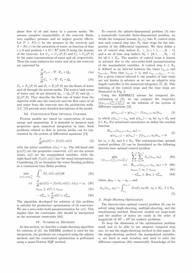
phase flow of oil and water in a porous media. Weassume complete immiscibility of the reservoir fluids,zero capillary pressure and we neglect gravity effects.Let P = P (t, r) be the pressure in the reservoir andS = S(t, r) be the saturation of water, as function of timet ≥ 0 and position r ∈ Ω ⊂ R3 with Ω being the domainof the reservoir. Let Cw = Cw(P, S) and Co = Co(P, S)be the mass concentrations of water and oil, respectively.Then the mass balances for water and oil in the reservoirare expressed by
∂
∂tCw= −∇ · Fw +Qw (1a)
∂
∂tCo = −∇ · Fo +Qo (1b)
Fw = Fw(P, S) and Fo = Fo(P, S) are the fluxes of waterand oil through the porous media. The source/sink termsof water and oil are denoted Qw = Qw(P, S) and Qo =Qo(P, S). They describe the flow rate of water from theinjection wells into the reservoir and the flow rates of oiland water from the reservoir into the production wells.[11]–[13] provide more detailed descriptions of the model.
III. Continuous-Time Optimal Control
Process models are based on conservation of mass,energy and momentum. It is desirable to preserve suchproperties upon numerical integration in time. Suchproblems related to flow in porous media can be rep-resented by the system of differential equations [13]
d
dtg(x(t)) = f(x(t), u(t)) (2)
with the initial condition x(t0) = x0. The left-hand sideg(x(t)) are the properties conserved, x(t) are the systemstates, u(t) are the manipulated variables, while theright-hand side f(x(t), u(t)) has the usual interpretation.Considering (2) we formulate the water flooding problemas a continuous time Bolza problem
min[x(t),u(t)]
tft0
∫ tf
t0
J(t, x(t), u(t))dt (3a)
s.t.d
dtg(x(t)) = f(x(t), u(t)), x(t0) = x0 (3b)
umin ≤ u(t) ≤ umax (3c)
− u∆min ≤d
dtu(t) ≤ u∆max (3d)
The algorithm developed for solution of this problemis suitable for production optimization of oil reservoirs.We use a zero-order-hold parameterization for u(t). Thisimplies that the constraints (3d) should be interpretedas the movement constraints (6d).
IV. Numerical Methods
In this section, we describe a single-shooting algorithmfor solution of (3). An ESDIRK method is used for theintegration, the gradients are computed using the adjointmethod, and the constrained optimization is performedusing a quasi-Newton SQP method.
To convert the infinite-dimensional problem (3) intoa numerically tractable finite-dimensional problem, wedivide the temporal domain [t0, tf ] into K control stepsand each control step into Nk time steps for the inte-gration of the differential equations. We then define aset of control step indices Ki = i, i + 1, . . . ,K − 1and a set of time step indices Nk = 0, 1, . . . , Nk − 1for all k ∈ K0. The number of control steps is knownin advance due to the zero-order-hold parametrizationof the manipulated variables. A control step k ∈ K0
is defined as an interval between the times tnk=0 andtnk=Nk
. Note that tn0=0 = t0 and tnK−1=NK−1= tf .
For a given control interval k, the number of time stepsare not known in advance as we use an adaptive steplength controller in the numerical integrator [7], [8]. Thisindexing of the control steps and the time steps areillustrated in Fig. 2.
Using the ESDIRK12 scheme for temporal dis-cretization of (2), we can compute the trajectoryxnk+1Nk−1
nk=0 K−1k=0 as the solution of the system of
difference equations [13]
g(xnk+1) = g(xnk)− f(xnk+1, uk)hnk
(4)
in which x(tnk) = xnk
and u(tnk) = uk for nk ∈ Nk and
k ∈ K0. For notational convenience we define the residualfunction
Rnk+1(xnk+1, xnk, uk) =
g(xnk+1)− g(xnk)− f(xnk+1, uk)hnk
= 0(5)
for nk ∈ Nk and k ∈ K0. The continuous-time optimalcontrol problem (3) can be formulated as the followingdiscrete-time optimal control problem
minxnk+1Nk−1
nk=0 ,ukK−1k=0
K−1∑
k=0
Nk−1∑
nk=0
Jnk(xnk
, uk) (6a)
s.t. Rnk+1(xnk+1, xnk, uk) = 0 (6b)
umin ≤ uk ≤ umax (6c)
− u∆min ≤ ∆uk ≤ u∆max (6d)
where ∆uk = uk − uk−1 and
Jnk(xnk
, uk) =
∫ tnk+1
tnk
J(x(t), uk)dt, nk ∈ Nk, k ∈ K0
(7)
A. Single-Shooting Optimization
The discrete-time optimal control problem (6) can besolved using single-shooting, multiple-shooting, and thesimultaneous method. Reservoir models are large-scaleand the number of states are easily in the order ofmagnitude of 105 − 106 for realistic problems.
To keep the dimension of the optimization problemsmall and to be able to use adaptive temporal stepsize, we use the single-shooting method in this paper. Inthe single-shooting method, the manipulated variables,u, are fixed at each iteration and used to solve thedifference equations (6b) numerically. Knowledge of the
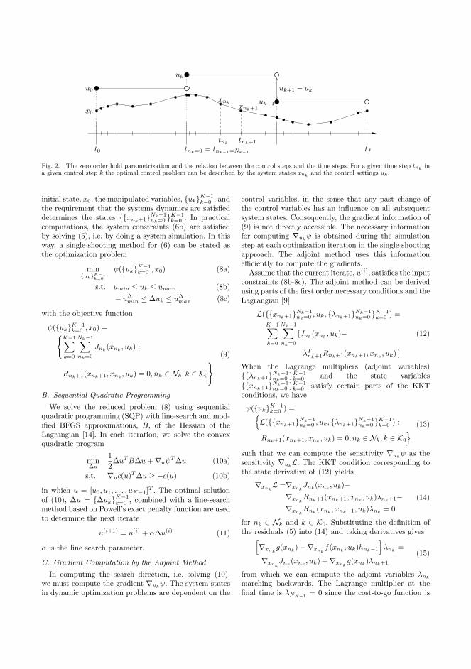
u0
x0
xnkxnk+1
uk+1
uk+1 − uk
tnktnk+1
uk
t0 tnk=0 = tnk−1=Nk−1tf
Fig. 2. The zero order hold parametrization and the relation between the control steps and the time steps. For a given time step tnk ina given control step k the optimal control problem can be described by the system states xnk and the control settings uk.
initial state, x0, the manipulated variables, ukK−1k=0 , and
the requirement that the systems dynamics are satisfieddetermines the states xnk+1Nk−1
nk=0 K−1k=0 . In practical
computations, the system constraints (6b) are satisfiedby solving (5), i.e. by doing a system simulation. In thisway, a single-shooting method for (6) can be stated asthe optimization problem
minukK−1
k=0
ψ(ukK−1k=0 , x0) (8a)
s.t. umin ≤ uk ≤ umax (8b)
− u∆min ≤ ∆uk ≤ u∆max (8c)
with the objective function
ψ(ukK−1k=0 , x0) =
K−1∑
k=0
Nk−1∑
nk=0
Jnk(xnk
, uk) :
Rnk+1(xnk+1, xnk, uk) = 0, nk ∈ Nk, k ∈ K0
(9)
B. Sequential Quadratic Programming
We solve the reduced problem (8) using sequentialquadratic programming (SQP) with line-search and mod-ified BFGS approximations, B, of the Hessian of theLagrangian [14]. In each iteration, we solve the convexquadratic program
min∆u
1
2∆uTB∆u+∇uψ
T∆u (10a)
s.t. ∇uc(u)T∆u ≥ −c(u) (10b)
in which u = [u0, u1, . . . , uK−1]T . The optimal solution
of (10), ∆u = ∆ukK−1k=0 , combined with a line-search
method based on Powell’s exact penalty function are usedto determine the next iterate
u(i+1) = u(i) + α∆u(i) (11)
α is the line search parameter.
C. Gradient Computation by the Adjoint Method
In computing the search direction, i.e. solving (10),we must compute the gradient ∇uk
ψ. The system statesin dynamic optimization problems are dependent on the
control variables, in the sense that any past change ofthe control variables has an influence on all subsequentsystem states. Consequently, the gradient information of(9) is not directly accessible. The necessary informationfor computing ∇uk
ψ is obtained during the simulationstep at each optimization iteration in the single-shootingapproach. The adjoint method uses this informationefficiently to compute the gradients.
Assume that the current iterate, u(i), satisfies the inputconstraints (8b-8c). The adjoint method can be derivedusing parts of the first order necessary conditions and theLagrangian [9]
L(xnk+1Nk−1nk=0 , uk, λnk+1Nk−1
nk=0 K−1k=0 ) =
K−1∑
k=0
Nk−1∑
nk=0
[Jnk(xnk
, uk)−
λTnk+1Rnk+1(xnk+1, xnk, uk) ]
(12)
When the Lagrange multipliers (adjoint variables)λnk+1Nk−1
nk=0 K−1k=0 and the state variables
xnk+1Nk−1nk=0 K−1
k=0 satisfy certain parts of the KKTconditions, we have
ψ(ukK−1k=0 ) =
L(xnk+1Nk−1nk=0 , uk, λnk+1Nk−1
nk=0 K−1k=0 ) :
Rnk+1(xnk+1, xnk, uk) = 0, nk ∈ Nk, k ∈ K0
(13)
such that we can compute the sensitivity ∇ukψ as the
sensitivity ∇ukL. The KKT condition corresponding to
the state derivative of (12) yields
∇xnkL =∇xnk
Jnk(xnk
, uk)−∇xnk
Rnk+1(xnk+1, xnk, uk)λnk+1−
∇xnkRnk
(xnk, xnk−1, uk)λnk
= 0
(14)
for nk ∈ Nk and k ∈ K0. Substituting the definition ofthe residuals (5) into (14) and taking derivatives gives
[∇xnk
g(xnk)−∇xnk
f(xnk, uk)hnk−1
]λnk
=
∇xnkJnk
(xnk, uk) +∇xnk
g(xnk)λnk+1
(15)
from which we can compute the adjoint variables λnk
marching backwards. The Lagrange multiplier at thefinal time is λNK−1
= 0 since the cost-to-go function is
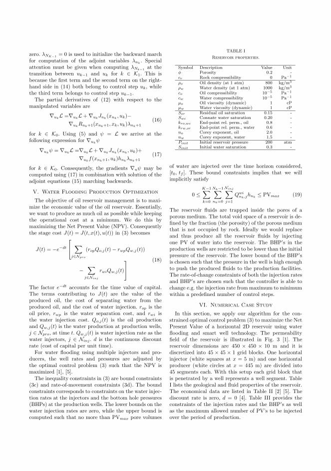
zero. λNK−1= 0 is used to initialize the backward march
for computation of the adjoint variables λnk. Special
attention must be given when computing λNk−1at the
transition between uk−1 and uk for k ∈ K1. This isbecause the first term and the second term on the right-hand side in (14) both belong to control step uk, whilethe third term belongs to control step uk−1.
The partial derivatives of (12) with respect to themanipulated variables are
∇ukL =∇uk
L+∇ukJnk
(xnk, uk)−
∇ukRnk+1(xnk+1, xk, uk)λnk+1
(16)
for k ∈ K0. Using (5) and ψ = L we arrive at thefollowing expression for ∇uk
ψ
∇ukψ = ∇uk
L =∇ukL+∇uk
Jnk(xnk
, uk)+
∇ukf(xnk+1, uk)hnk
λnk+1
(17)
for k ∈ K0. Consequently, the gradients ∇uψ may becomputed using (17) in combination with solution of theadjoint equations (15) marching backwards.
V. Water Flooding Production Optimization
The objective of oil reservoir management is to maxi-mize the economic value of the oil reservoir. Essentially,we want to produce as much oil as possible while keepingthe operational cost at a minimum. We do this bymaximizing the Net Present Value (NPV). Consequentlythe stage cost J(t) = J(t, x(t), u(t)) in (3) becomes
J(t) = −e−dt
∑
j∈Npro
(ropQo,j(t)− rwpQw,j(t))
−∑
j∈Ninj
rwiQw,j(t)
(18)
The factor e−dt accounts for the time value of capital.The terms contributing to J(t) are the value of theproduced oil, the cost of separating water from theproduced oil, and the cost of water injection. rop is theoil price, rwp is the water separation cost, and rwi isthe water injection cost. Qo,j(t) is the oil productionand Qw,j(t) is the water production at production wells,j ∈ Npro, at time t. Qw,j(t) is water injection rate as thewater injectors, j ∈ Ninj . d is the continuous discountrate (cost of capital per unit time).
For water flooding using multiple injectors and pro-ducers, the well rates and pressures are adjusted bythe optimal control problem (3) such that the NPV ismaximized [1], [5].
The inequality constraints in (3) are bound constraints(3c) and rate-of-movement constraints (3d). The boundconstraints corresponds to constraints on the water injec-tion rates at the injectors and the bottom hole pressures(BHPs) at the production wells. The lower bounds on thewater injection rates are zero, while the upper bound iscomputed such that no more than PVmax pore volumes
TABLE I
Reservoir properties.
Symbol Description Value Unitφ Porosity 0.2 -cr Rock compressibility 0 Pa−1
ρo Oil density (at 1 atm) 800 kg/m3
ρw Water density (at 1 atm) 1000 kg/m3
co Oil compressibility 10−5 Pa−1
cw Water compressibility 10−5 Pa−1
µo Oil viscosity (dynamic) 1 cPµw Water viscosity (dynamic) 1 cPSor Residual oil saturation 0.15 -Swc Connate water saturation 0.20 -kro,wc End-point rel. perm., oil 0.8 -krw,or End-point rel. perm., water 0.6 -no Corey exponent, oil 2.0 -nw Corey exponent, water 1.5 -Pinit Initial reservoir pressure 200 atmSinit Initial water saturation 0.3 -
of water are injected over the time horizon considered,[t0, tf ]. These bound constraints implies that we willimplicitly satisfy
0 ≤K−1∑
k=0
Nk−1∑
nk=0
Ninj∑
j=1
Qwink,j
hnk≤ PVmax (19)
The reservoir fluids are trapped inside the pores of aporous medium. The total void space of a reservoir is de-fined by the fraction (the porosity) of the porous mediumthat is not occupied by rock. Ideally we would replaceand thus produce all the reservoir fluids by injectingone PV of water into the reservoir. The BHP’s in theproduction wells are restricted to be lower than the initialpressure of the reservoir. The lower bound of the BHP’sis chosen such that the pressure in the well is high enoughto push the produced fluids to the production facilities.The rate-of-change constraints of both the injection ratesand BHP’s are chosen such that the controller is able tochange e.g. the injection rate from maximum to minimumwithin a predefined number of control steps.
VI. Numerical Case Study
In this section, we apply our algorithm for the con-strained optimal control problem (3) to maximize the NetPresent Value of a horizontal 2D reservoir using waterflooding and smart well technology. The permeabilityfield of the reservoir is illustrated in Fig. 3 [1]. Thereservoir dimensions are 450 × 450 × 10 m and it isdiscretized into 45 × 45 × 1 grid blocks. One horizontalinjector (white squares at x = 5 m) and one horizontalproducer (white circles at x = 445 m) are divided into45 segments each. With this setup each grid block thatis penetrated by a well represents a well segment. TableI lists the geological and fluid properties of the reservoir.The economical data are listed in Table II [2] [5]. Thediscount rate is zero, d = 0 [4]. Table III provides theconstraints of the injection rates and the BHP’s as wellas the maximum allowed number of PV’s to be injectedover the period of production.
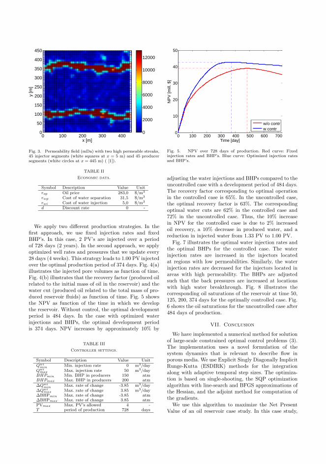
x [m]
y [m
]
0 100 200 300 4000
50
100
150
200
250
300
350
400
450
0
2000
4000
6000
8000
10000
12000
Fig. 3. Permeability field (mDa) with two high permeable streaks,45 injector segments (white squares at x = 5 m) and 45 producersegments (white circles at x = 445 m) ( [1]).
TABLE II
Economic data.
Symbol Description Value Unitrop Oil price 283,0 $/m3
rwp Cost of water separation 31,5 $/m3
rwi Cost of water injection 5,0 $/m3
d Discount rate 0 -
We apply two different production strategies. In thefirst approach, we use fixed injection rates and fixedBHP’s. In this case, 2 PV’s are injected over a periodof 728 days (2 years). In the second approach, we applyoptimized well rates and pressures that we update every28 days (4 weeks). This strategy leads to 1.00 PV injectedover the optimal production period of 374 days. Fig. 4(a)illustrates the injected pore volumes as function of time.Fig. 4(b) illustrates that the recovery factor (produced oilrelated to the initial mass of oil in the reservoir) and thewater cut (produced oil related to the total mass of pro-duced reservoir fluids) as function of time. Fig. 5 showsthe NPV as function of the time in which we developthe reservoir. Without control, the optimal developmentperiod is 484 days. In the case with optimized waterinjections and BHPs, the optimal development periodis 374 days. NPV increases by approximately 10% by
TABLE III
Controller settings.
Symbol Description Value UnitQwi
min Min. injection rate 0 m3/dayQwi
max Max. injection rate 50 m3/dayBHPmin Min. BHP in producers 150 atmBHPmax Max. BHP in producers 200 atm∆Qwi
min Max. rate of change -3.85 m3/day∆Qwi
max Max. rate of change 3.85 m3/day∆BHPmin Max. rate of change -3.85 atm∆BHPmax Max. rate of change 3.85 atmPVmax Max. PV’s allowed 4 -T period of production 728 days
0 100 200 300 400 500 600 7000
10
20
30
40
50
Time [day]
NP
V [m
ill. $
]
w/o contrw contr
Fig. 5. NPV over 728 days of production. Red curve: Fixedinjection rates and BHP’s. Blue curve: Optimized injection ratesand BHP’s.
adjusting the water injections and BHPs compared to theuncontrolled case with a development period of 484 days.The recovery factor corresponding to optimal operationin the controlled case is 65%. In the uncontrolled case,the optimal recovery factor is 63%. The correspondingoptimal water cuts are 62% in the controlled case and72% in the uncontrolled case. Thus, the 10% increasein NPV for the controlled case is due to 2% increasedoil recovery, a 10% decrease in produced water, and areduction in injected water from 1.33 PV to 1.00 PV.
Fig. 7 illustrates the optimal water injection rates andthe optimal BHPs for the controlled case. The waterinjection rates are increased in the injectors locatedat regions with low permeabilities. Similarly, the waterinjection rates are decreased for the injectors located inareas with high permeability. The BHPs are adjustedsuch that the back pressures are increased at locationswith high water breakthrough. Fig. 8 illustrates thecorresponding oil saturations of the reservoir at time 50,125, 200, 374 days for the optimally controlled case. Fig.6 shows the oil saturations for the uncontrolled case after484 days of production.
VII. Conclusion
We have implemented a numerical method for solutionof large-scale constrained optimal control problems (3).The implementation uses a novel formulation of thesystem dynamics that is relevant to describe flow inporous media. We use Explicit Singly Diagonally ImplicitRunge-Kutta (ESDIRK) methods for the integrationalong with adaptive temporal step sizes. The optimiza-tion is based on single-shooting, the SQP optimizationalgorithm with line-search and BFGS approximations ofthe Hessian, and the adjoint method for computation ofthe gradients.
We use this algorithm to maximize the Net PresentValue of an oil reservoir case study. In this case study,

0 100 200 300 400 500 600 7000
0.5
1
1.5
2
Time [day]
PV
w/o contrw contr
(a) PV injected.
0 100 200 300 400 500 600 7000
0.2
0.4
0.6
Time [day]
Rec
over
y
w/o contrw contr
0 100 200 300 400 500 600 7000
0.2
0.4
0.6
Time [day]
Wat
er c
ut
w/o contrw contr
(b) Recovery factor (top) and water cut (bottom).
Fig. 4. Production data over 728 days of production. Red: Fixed injection rates and BHP’s. Blue: Optimized injection rates and BHP’s.
Time [day]
y [m
]
0 200 400 600
5
10
15
20
25
30
35
40
45
12
14
16
18
20
22
24
26
28
30
32
(a) Individual injection rates (m3/day) of 45 injectors.
Time [day]
y [m
]
0 200 400 6000
50
100
150
200
250
300
350
400
450
150
155
160
165
170
175
(b) Individual BHP’s (atm) of 45 producers.
Fig. 7. Injection rates and BHP’s over 728 days of production, updated each 28 days. The injectors and producers are depicted in Figure3.
we use water flooding to produce the oil. The developedlarge-scale constrained optimal control algorithm com-putes the optimal profiles of water injection rates andthe bottom hole pressures. Compared to the uncontrolledcase, the Net Present Value in the controlled case in-creases by 10%. This figure demonstrates a significanteconomic potential of applying smart well technologyalong with constrained optimal control in oil reservoirmanagement.
References
[1] D. Brouwer and J.-D. Jansen, “Dynamic optimization of wa-terflooding with smart wells using optimal control theory,”SPE Journal, vol. 9, no. 4, pp. 391–402, 2004.
[2] J. F. B. M. Kraaijevanger, P. J. Egberts, J. R. Valstar, andH. W. Buurman,“Optimal waterflood design using the adjointmethod,” in SPE Reservoir Simulation Symposium. Houston,Texas, U.S.A.: Society of Petroleum Engineers, 2007.
[3] J.-D. Jansen, O. H. Bosgra, and P. M. Van den Hof, “Model-based control of multiphase flow in subsurface oil reservoirs,”Journal of Process Control, vol. 18, no. 9, pp. 846–855, Oct.2008.
[4] P. Sarma, W. H. Chen, L. J. Durlofsky, and K. Aziz, “Produc-tion optimization with adjoint models under nonlinear control-state path inequality constraints,” SPE Reservoir Evaluation& Engineering, vol. 11, no. 2, pp. 326–339, 2008.
[5] J.-D. Jansen, R. Brouwer, and S. G. Douma, “Closed loopreservoir management,” in SPE Reservoir Simulation Sympo-sium. The Woodlands, Texas: Society of Petroleum Engi-neers, 2009.
[6] E. Suwartadi, S. Krogstad, and B. A. Foss, “On state con-straints of adjoint optimization in oil reservoir waterflooding,”in SPE/EAGE Reservoir Characterization and SimulationConference. Abu Dhabi, UAE: Society of Petroleum Engi-neers, 2009.
[7] C. Volcker, J. B. Jørgensen, P. G. Thomsen, and E. H. Stenby,“Adaptive stepsize control in implicit runge-kutta methodsfor reservoir simulation,” 9th International Symposium onDynamics and Control of Process Systems, 2010.
[8] ——,“Explicit singly diagonally implicit runge-kutta methods

x [m]
y [m
]
0 200 400 6000
5
10
15
20
25
30
35
40
45
0.15
0.2
0.25
0.3
0.35
0.4
0.45
0.5
0.55
0.6
0.65
(a) 0.14 PV injected after 50 days.
x [m]
y [m
]
0 200 400 6000
5
10
15
20
25
30
35
40
45
0.15
0.2
0.25
0.3
0.35
0.4
0.45
0.5
0.55
0.6
0.65
(b) 0.41 PV injected after 125 days.
x [m]
y [m
]
0 200 400 6000
5
10
15
20
25
30
35
40
45
0.15
0.2
0.25
0.3
0.35
0.4
0.45
0.5
0.55
0.6
0.65
(c) 0.64 PV injected after 200 days.
x [m]
y [m
]
0 200 400 6000
50
100
150
200
250
300
350
400
450
0.15
0.2
0.25
0.3
0.35
0.4
0.45
0.5
0.55
0.6
0.65
(d) 1.00 PV injected after 374 days.
Fig. 8. Oil saturations after 50, 125, 200 and 374 days of production using optimized injection rates and BHP’s.
and adaptive stepsize control for reservoir simulation,” 12thEuropean Conference on the Mathematics of Oil Recovery,2010.
[9] J. B. Jørgensen, “Adjoint sensitivity results for predictive con-trol, state- and parameter-estimation with nonlinear models,”in Proceedings of the European Control Conference 2007, Kos,Greece, July 2-5 2007, pp. 3649–3656.
[10] P. Sarma, K. Aziz, and L. Durlofsky, “Implementation ofadjoint solution for optimal control of smart wells,” in SPEReservoir Simulation Symposium. The Woodlands, Texas:2005,. Society of Petroleum Engineers Inc., 2005.
[11] K. Aziz and A. Settari, Petroleum Reservoir Simulation,1st ed. London: Applied Science Publishers Ltd, 1979.
[12] Z. Chen, Reservoir Simulation : Mathematical Techniques inOil Recovery. Philadelphia: Society for Industrial and AppliedMathematics (SIAM), 2007.
[13] C. Volcker, J. B. Jørgensen, P. G. Thomsen, and E. H. Stenby,“Simulation of subsurface two-phase flow in an oil reservoir,”in Proceedings of the European Control Conference 2009,Budapest, Hungary, August 23-26 2009, pp. 1221–1226.
[14] J. Nocedal and S. J. Wright, Numerical Optimization, 2nd ed.New York, USA: Springer Series in Operations Research andFinancial Engineering, 2006.
x [m]
y [m
]
0 200 400 6000
50
100
150
200
250
300
350
400
450
0.15
0.2
0.25
0.3
0.35
0.4
0.45
0.5
0.55
0.6
0.65
Fig. 6. Oil saturation 484 days of production using fixed injectionrates and BHP’s.