Embed Size (px)
Citation preview

Stochastic Hub and Spoke Networks
Edward Eric Hult
Homerton College
Judge Business School
University of Cambridge
A thesis submitted for the degree of
Doctor of Philosophy
2011

I would like to dedicate this thesis to my loving wife who has been by my side through
all my ups and downs, who has supported me and helped me, during the entire course
of my Ph.D., which has been both a very emotional and intellectually challenging
journey. Without her, things would not be the same.
i

Declaration of Originality
I declare, as the author of this thesis, the work and research presented here is, to the best
of my knowledge and belief, original except where due acknowledgement, in accordance
with the standard referencing practices, is made in the text of the thesis. I certify that the
work has not been previously submitted for a degree or diploma at any other institution.
I declare that no ideas, techniques, or any other material from the work of other people is
included in my thesis where full acknowledgement is not made with the exception of the
work contributed by my two supervisors Daniel Ralph and Houyuan Jiang in Chapter
2. Chapter 2 is a co-authored paper, where I am the first author, together with my two
supervisors. Apart from standard supervision input, both Daniel Ralph and Houyuan
Jiang have contributed with the write up of Chapter 2 and in addition Houyuan Jiang
has assisted in producing the majority of the C++ code referred to in this chapter.
Edward E. Hult, 18 May 2011
ii

Acknowledgement
It is difficult to overstate my gratitude to my first and second Ph.D. supervisors, Prof.
Daniel Ralph and Dr. Houyuan Jiang, for all their invaluable help. I have learned a
lot from them during my time at Cambridge and I would like to thank them for always
challenging me and questioning me, teaching me to always make sure I could fully
motivate and understand any new ideas I brought to the table. I would like to thank
them for all the great, lively, and very useful meetings we have had over the last few
years and for all their useful tips and tricks for attacking and overcoming any problems
which have been encountered along the way. Most importantly I would like to thank
them for all their time they have given me and all their patience they have shown me,
during the course of my Ph.D. degree.
I would also like to thank my sister in law, Britt Hult, for her time, help and useful
comments, proof reading this thesis.
Additionally, I would like to thank my friends and family who have been there for me,
especially my parents who have always inspired me and motivated me to always stay
the course, no matter how hard things get.
iii
Abstract
Transportation systems such as mail, freight, passenger and even telecommunication
systems most often employ a hub and spoke network structure since correctly designed
they give a strong balance between high service quality and low costs resulting in an
economically competitive operation. In addition, consumers are increasingly demanding
fast and reliable transportation services, with services such as next day deliveries and
fast business and pleasure trips becoming highly sought after. This makes finding an
efficient design of a hub and spoke network of the utmost importance for any competing
transportation company. However real life situations are complicated, dynamic and
often require responses to many different fixed and random events. Therefore modeling
the question of what is an optimal hub and spoke network structure and finding an
optimal solution is very difficult. Due to this, many researchers and practitioners alike
make several assumptions and simplifications on the behavior of such systems to allow
mathematical models to be formulated and solved optimally or near optimally within
a practical timeframe. Some assumptions and simplifications can however result in
practically poor network design solutions being found. This thesis contributes to the
research of hub and spoke networks by introducing new stochastic models and fast
solution algorithms to help bridge the gap between theoretical solutions and designs
that are useful in practice.
Three main contributions are made in the thesis. First, in Chapter 2, a new formulation
and solution algorithms are proposed to find exact solutions to a stochastic p-hub center
problem. The stochastic p-hub center problem is about finding a network structure,
where travel times on links are stochastic, which minimizes the longest path in the
network to give fast delivery guarantees which will hold for some given probability.
Second, in Chapter 3, the stochastic p-hub center problem is looked at using a new
methodological approach which gives more realistic solutions to the network structures
when applied to real life situations. In addition a new service model is proposed where
volume of flow is also accounted for when considering the stochastic nature of travel
times on links. Third, in Chapter 4, stochastic volume is considered to account for
capacity constraints at hubs and, de facto, reduce the costs embedded in excessive hub
volumes. Numerical experiments and results are conducted and reported for all models
in all chapters which demonstrate the efficiency of the new proposed approaches.
iv
Contents
1 Introduction 1
1.1 The Hub and Spoke Network Design . . . . . . . . . . . . . . . . . . . . 1
1.2 Contributions . . . . . . . . . . . . . . . . . . . . . . . . . . . . . . . . . 5
1.3 Literature Review . . . . . . . . . . . . . . . . . . . . . . . . . . . . . . . 6
2 Paper One 10
2.1 Introduction . . . . . . . . . . . . . . . . . . . . . . . . . . . . . . . . . . 11
2.1.1 Literature review . . . . . . . . . . . . . . . . . . . . . . . . . . . 13
2.2 The Stochastic Hub Center Problem and a Reformulation . . . . . . . . . 15
2.3 Solution Methods . . . . . . . . . . . . . . . . . . . . . . . . . . . . . . . 19
2.3.1 SpHCP-Pull, preprocessing . . . . . . . . . . . . . . . . . . . . . . 19
2.3.2 SpHCP-Push, separation algorithm . . . . . . . . . . . . . . . . . 20
2.4 Numerical Results . . . . . . . . . . . . . . . . . . . . . . . . . . . . . . . 22
2.5 Conclusion . . . . . . . . . . . . . . . . . . . . . . . . . . . . . . . . . . . 28
3 Paper Two 31
3.1 Introduction . . . . . . . . . . . . . . . . . . . . . . . . . . . . . . . . . . 32
3.1.1 Literature review . . . . . . . . . . . . . . . . . . . . . . . . . . . 35
3.2 New Methodological Approach to a Stochastic p-hub Center Problem . . 38
v

3.2.1 Variable departure times . . . . . . . . . . . . . . . . . . . . . . . 39
3.2.2 Preset departure times . . . . . . . . . . . . . . . . . . . . . . . . 46
3.2.3 Numerical results . . . . . . . . . . . . . . . . . . . . . . . . . . . 51
3.3 The Service Cost Problem . . . . . . . . . . . . . . . . . . . . . . . . . . 56
3.3.1 Stochastic formulation . . . . . . . . . . . . . . . . . . . . . . . . 57
3.3.2 Reformulations . . . . . . . . . . . . . . . . . . . . . . . . . . . . 58
3.3.3 Numerical results . . . . . . . . . . . . . . . . . . . . . . . . . . . 61
3.4 Conclusion . . . . . . . . . . . . . . . . . . . . . . . . . . . . . . . . . . . 64
4 Paper Three 70
4.1 Introduction . . . . . . . . . . . . . . . . . . . . . . . . . . . . . . . . . . 71
4.1.1 Literature review . . . . . . . . . . . . . . . . . . . . . . . . . . . 73
4.2 The Stochastic Capacitated Single Allocation Hub Location Problem . . 76
4.3 Sample Average Approximation . . . . . . . . . . . . . . . . . . . . . . . 80
4.3.1 Convergence . . . . . . . . . . . . . . . . . . . . . . . . . . . . . . 81
4.4 Solution Method . . . . . . . . . . . . . . . . . . . . . . . . . . . . . . . 83
4.5 Numerical Results . . . . . . . . . . . . . . . . . . . . . . . . . . . . . . . 86
4.5.1 Main run . . . . . . . . . . . . . . . . . . . . . . . . . . . . . . . 87
4.5.2 Effects of using different sample sizes . . . . . . . . . . . . . . . . 89
4.5.3 Stochastic vs. deterministic solutions . . . . . . . . . . . . . . . . 91
4.6 Conclusion . . . . . . . . . . . . . . . . . . . . . . . . . . . . . . . . . . . 94
5 Conclusion 95
5.1 Future Research . . . . . . . . . . . . . . . . . . . . . . . . . . . . . . . . 97
vi
List of Figures
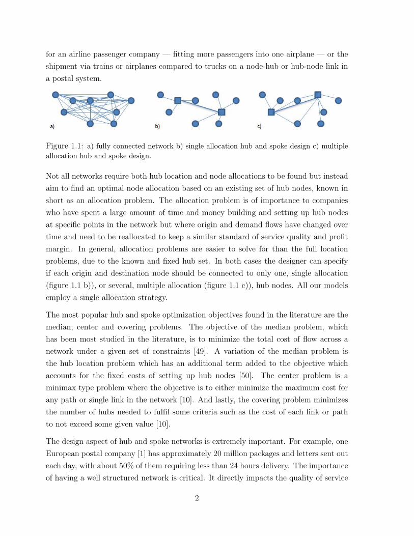
1.1 a) fully connected network b) single allocation hub and spoke design c) multiple
allocation hub and spoke design. . . . . . . . . . . . . . . . . . . . . . . . . 2
2.1 Performance of CPU times for SpHCPL, SpHCPL-Pull, and SpHCPL-Push:
The top panel for the CAB dataset and the bottom panel for the AP dataset. 27
2.2 Sensitivity results of the CPU times in coefficient of variation ν and service
level parameter γ for test example AP 25.2. . . . . . . . . . . . . . . . . . . 28
3.1 Origin-destination path via hub nodes. . . . . . . . . . . . . . . . . . . . . . 32
3.2 Departure times for a deterministic model. . . . . . . . . . . . . . . . . . . . 34
3.3 Example network. . . . . . . . . . . . . . . . . . . . . . . . . . . . . . . . 66
3.4 Critical section of a network. . . . . . . . . . . . . . . . . . . . . . . . . . . 67
3.5 Decreasing values. . . . . . . . . . . . . . . . . . . . . . . . . . . . . . . . 68
4.1 Origin - destination path. . . . . . . . . . . . . . . . . . . . . . . . . . . . 71
4.2 Cumulative distribution graph for total volume flowing into a hub, showing the
VaRγ , CVaRγ and the hub capacity, Γ. . . . . . . . . . . . . . . . . . . . . 79
4.3 Number of times an optimal solution was found from 100 different runs for
each sample size S = {100, 200, 400, 600, 800}. . . . . . . . . . . . . . . . . . 89
4.4 Average solution times over ten different runs for each sample size S =
{100, 200, 300, 400, 500, 600, 700, 800, 900, 1000}. . . . . . . . . . . . . . . . . 90
vii
List of Tables
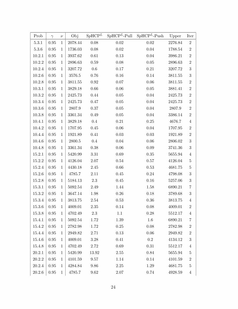
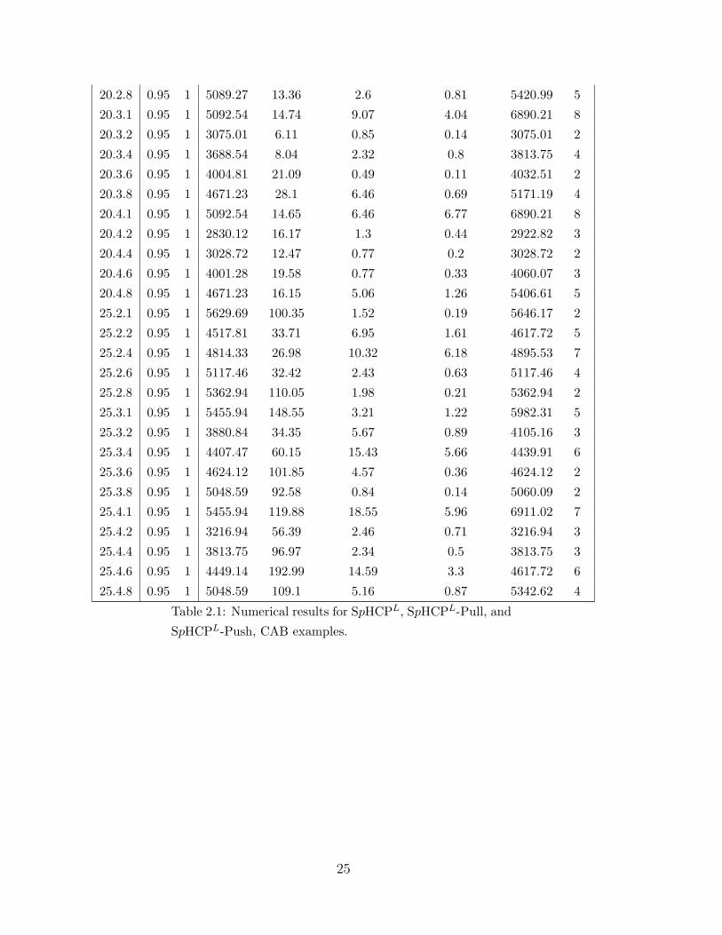
2.1 Numerical results for SpHCPL, SpHCPL-Pull, and SpHCPL-Push, CAB
examples. . . . . . . . . . . . . . . . . . . . . . . . . . . . . . . . . . . . 25
2.2 Numerical results for SpHCPL, SpHCPL-Pull, and SpHCPL-Push, AP
examples. . . . . . . . . . . . . . . . . . . . . . . . . . . . . . . . . . . . 26
3.1 Departure times from each ghost node kθ, θ = {1, ..., 4}, to nodes m,
m = {Paris, Rome, New York}. . . . . . . . . . . . . . . . . . . . . . . . 49
3.2 Numerical results for SpHCPDVL , CAB examples. . . . . . . . . . . . . . 52
3.3 Numerical results for SpHCPDVL , AP examples. . . . . . . . . . . . . . . 53
3.4 Test results for SpHCPDVL using different step sizes. . . . . . . . . . . . . 54
3.5 Numerical results for SpHCPDFL , CAB examples. . . . . . . . . . . . . . 55
3.6 Numerical results for SpHCPDFL AP, examples. . . . . . . . . . . . . . . . 56
3.7 Numerical results for SCP CAB, examples. . . . . . . . . . . . . . . . . . 63
3.8 Numerical results for SCP AP, examples. . . . . . . . . . . . . . . . . . . 64
4.1 Numerical results for AP examples 10LL - 25TT, S = 400. . . . . . . . . 88
4.2 Numerical results for AP examples 40LL - 50TT, S = 200. . . . . . . . . 89
4.3 Expected capacity breaches at different hubs for AP 20 examples. . . . . 92
4.4 Cost and capacity breach differences for AP 20LT and 20TT examples. . 93
viii

Chapter 1
Introduction
Different network systems are found everywhere in our world, from DNA strands which
make up life to the early Roman water management and road network systems to modern
day transportation systems and social networks such as Facebook and Twitter. The
topic of this PhD thesis is an in-depth research study on a specific type of network
system known as hub and spoke networks. Specifically the design phase of such systems
is studied considering optimization tools and solution procedures. Special emphasis is
made on the stochastic properties of such networks and how they can be incorporated
into solvable mathematical programming models.
1.1 The Hub and Spoke Network Design
Hub and spoke networks are used and found in many different areas, such as shipping and
postal mail systems, air and rail transportation, and telecommunication networks [3, 13].
Given multiple origin nodes which each need to be connected to multiple destination
nodes it becomes economically and practically infeasible to connect every origin and
destination node (OD pair) with a direct single link connection. Instead a hub and
spoke network aggregates multiple origin flows at a single hub node where the high
volume aggregated flow travels from one hub to another via a hub-hub link as shown
in figure 1.1, all hub nodes are assumed to be fully connected. Arriving at the second
hub node the flow then gets split up and sorted for shipment to each of its respective
destination nodes. Travel or shipment along a hub-hub link is often quicker and less
expensive per unit flow due to the aggregation of flows. Examples include larger jets
1
for an airline passenger company — fitting more passengers into one airplane — or the
shipment via trains or airplanes compared to trucks on a node-hub or hub-node link in
a postal system.
Figure 1.1: a) fully connected network b) single allocation hub and spoke design c) multipleallocation hub and spoke design.
Not all networks require both hub location and node allocations to be found but instead
aim to find an optimal node allocation based on an existing set of hub nodes, known in
short as an allocation problem. The allocation problem is of importance to companies
who have spent a large amount of time and money building and setting up hub nodes
at specific points in the network but where origin and demand flows have changed over
time and need to be reallocated to keep a similar standard of service quality and profit
margin. In general, allocation problems are easier to solve for than the full location
problems, due to the known and fixed hub set. In both cases the designer can specify
if each origin and destination node should be connected to only one, single allocation
(figure 1.1 b)), or several, multiple allocation (figure 1.1 c)), hub nodes. All our models
employ a single allocation strategy.
The most popular hub and spoke optimization objectives found in the literature are the
median, center and covering problems. The objective of the median problem, which
has been most studied in the literature, is to minimize the total cost of flow across a
network under a given set of constraints [49]. A variation of the median problem is
the hub location problem which has an additional term added to the objective which
accounts for the fixed costs of setting up hub nodes [50]. The center problem is a
minimax type problem where the objective is to either minimize the maximum cost for
any path or single link in the network [10]. And lastly, the covering problem minimizes
the number of hubs needed to fulfil some criteria such as the cost of each link or path
to not exceed some given value [10].
The design aspect of hub and spoke networks is extremely important. For example, one
European postal company [1] has approximately 20 million packages and letters sent out
each day, with about 50% of them requiring less than 24 hours delivery. The importance
of having a well structured network is critical. It directly impacts the quality of service
2

provided where design decisions affect economic viability through cost and reliability of
deliveries. The choice of optimal hub locations and/or node allocations is however not
an easy task. The economy of scale on hub-hub links make hub and node allocation
choices far from obvious with the addition of accounting for many other factors which
are not always clear or easy to capture. Each system has its own unique characteristics
and often has multiple dynamic and unpredictable or random elements to it which need
to be considered. On the other hand, good hub and spoke network designs can still be
found by simplifying some appropriate network characteristics. However, as can be seen
throughout the hub and spoke literature, as we will demonstrate in Sections 1.3, 2.1.1,
3.1.1 and 4.1.1 by citing some of the academic literature, the computational difficulty
of solving even simple hub and spoke design problems has led to a somewhat narrow
research output. This research pool can be divided up into two different focus areas.
The first aims to create new or expand on existing models in an attempt to create more
realistic representations of real life systems. The second focuses on reformulating and/or
constructing new solution methods to existing models to improve upon the computa-
tional performance allowing larger sized networks to be solved. These areas of research
are of importance to hub and spoke design since they both, in their own right, contribute
to bridging the gap between small solvable theoretical models and large computationally
infeasible real life systems. This thesis contributes to both of these research areas by
working in the realm of stochastic optimization.
Due to the complexity of solving for optimal hub and spoke network designs, the vast
majority of the literature simplifies all stochastic events which take place in a real life
system by assuming average values [6, 9, 10, 12, 16, 16, 17, 18, 20, 22, 23, 24, 25, 27, 28,
36, 37, 38, 40, 41, 45, 47, 48, 50, 53, 49, 52, 56, 60, 61, 66, 67, 68, 70, 71, 72, 74, 80],
[alternatively see the two literature review papers [3, 13] which have over 100 references
each of papers considering deterministic hub and spoke network designs]. Even though
such simplification may be sensible in some cases, there are many situations where such
simplifications can result in poor designs due to the flaw of averages [62]. The flaw of
averages simply states: “plans based on the assumption that average conditions will
occur are usually wrong” [63]. In optimal decision making, such as in hub and spoke
network design, Rosenhead et al. [59] divided decision making into three categories —
certainty, risk and uncertainty. All deterministic situations are classified as certainty,
i.e. everything is known and no randomness exists. For risk and uncertainty situations,
random events occur, which is the norm in everyday life. For risk, the random events are
governed by probability distributions which are known. For uncertainty, no properties
3
of the random events are available. The facility location literature, among others, has
picked up on the importance of incorporating stochastic optimization and has produced
a vast pool of research papers covering the different decision making environments [69].
For hub and spoke network design models, risk and uncertainty research is very limited
but is nonetheless very important to consider, see for example the Appendix of Chapter
3: “Example A: Importance of considering stochastic link travel times”. The three
papers presented in this thesis all deal within the risk environment.
Risk modeling has been around for some time and has played a vital role in financial
modeling. In 1952 Markowitz [46] introduced modern portfolio theory by studying the
trade off between risk and expected return. The models included either fixing risk
and maximizing the expected return or fixing the expected return and minimizing risk.
By changing the fixed parameters, one can create an efficient frontier and then choose
the optimal portfolio depending on one’s risk preference. The random events in these
models follow a Gaussian distribution and the risk is defined as the variance. Another,
and probably the most common, risk measure in finance is value-at-risk (VaR) which
first became widely used in the early 1990s following the stock market crash of 1987,
also known as Black Monday [35]. The idea behind VaR is to minimize the value, φ,
which a loss should not exceed for a given probability level γ. In general this differs from
a mean-variance model, where one either minimizes the risk or maximizes the expected
return, and instead finds the setup which gives the smallest loss for a given confidence
interval. Although VaR gives a minimum value φ which should not be exceeded for some
probability, it does not account for how bad things might get when φ is exceeded. To be
able to account for this, Rockafellar and Uryasev [57] introduced conditional value-at-
risk (CVaR). CVaR states that for a lower value φ, such that the cost does not exceed φ
with a probability γ, then CVaR is the expected value when φ is exceeded. For example,
if 95% of the time it takes a postal company less than 24 hours to deliver a package from
A to B, then CVaR calculates the expected time when the delivery exceeds 24 hours.
Since CVaR is the expected value when VaR is breached, we automatically get a small
VaR value as well when we minimize CVaR. On the other end, if whatever happens
when some value is breached does not incur extra costs based on the size of the breach,
but instead results in some known fixed cost, one can instead minimize the probability
of exceeding such a value by formulating a minimum probability model. This list is far
from comprehensive but highlights some key risk measures which can be used for hub
and spoke design problems.
4
1.2 Contributions
We present three different stand alone papers which make up Chapters 2, 3 and 4 of
this thesis. Our first paper is a computational contribution applied on a stochastic
uncapacitated single allocation p-hub center problem proposed in Sim et al. [65]. The
problem considers the stochastic nature of travel times on links and the authors construct
heuristic methods to find approximate solutions to networks of up to 40 nodes in size.
We contribute to this problem by finding exact solutions to 50 node networks. We first
propose a new and more efficient formulation to the problem in [65] which allows exact
solutions to be found for networks up to 25 nodes in size. We then preprocess the model,
reducing its size, which further allows us to solve 40 node networks exactly. Lastly we
propose a separation algorithm which effectively solves 50 node networks to optimality.
Our second paper, Chapter 3, further extends the methodology proposed in [65] and used
in Chapter 2. We show that specifically accounting for departure times at hub nodes in
the model can lead to better and more practical network designs. Two different models
are proposed where one allows optimal departure times to be solved for while the other
assumes a fixed list of departure times are available for each potential hub to hub link.
Solutions are found by reformulating the models into an approximate linear model, using
a step function, and an equivalent linear model, respectively, by assuming independent
normal distributions on the link travel times. Further we prove that the optimal location-
allocation solutions to the approximation model are a subset of the optimal solutions to
the original stochastic model when the step sizes are small enough. Computational tests
are also presented which demonstrate the effectiveness of the solution formulations. In
addition we also propose a new model in the second paper for a hub allocation problem.
The objective of this model is to minimize the probability of all paths of over exceeding
some guaranteed delivery time. There is a cost function associated with each path which
accounts for the volume along the paths. The purpose of the model is to maximize the
percent of total packages which can be delivered on time as opposed to paths which
deliver within some probability on time. Three solution approaches are also presented
and tested for this new model where fixed departure times are assumed.
In our third paper, Chapter 4, we consider a capacitated single allocation hub location
problem with stochastic demand. Most real life systems have some type of capacity
constraints on the amount of incoming flow a hub can handle. Considering the daily
fluctuations of flow volume is important. Knowing that the average traffic flow falls
5
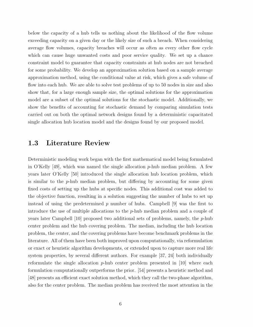
below the capacity of a hub tells us nothing about the likelihood of the flow volume
exceeding capacity on a given day or the likely size of such a breach. When considering
average flow volumes, capacity breaches will occur as often as every other flow cycle
which can cause huge unwanted costs and poor service quality. We set up a chance
constraint model to guarantee that capacity constraints at hub nodes are not breached
for some probability. We develop an approximation solution based on a sample average
approximation method, using the conditional value at risk, which gives a safe volume of
flow into each hub. We are able to solve test problems of up to 50 nodes in size and also
show that, for a large enough sample size, the optimal solutions for the approximation
model are a subset of the optimal solutions for the stochastic model. Additionally, we
show the benefits of accounting for stochastic demand by comparing simulation tests
carried out on both the optimal network designs found by a deterministic capacitated
single allocation hub location model and the designs found by our proposed model.
1.3 Literature Review
Deterministic modeling work began with the first mathematical model being formulated
in O’Kelly [49], which was named the single allocation p-hub median problem. A few
years later O’Kelly [50] introduced the single allocation hub location problem, which
is similar to the p-hub median problem, but differing by accounting for some given
fixed costs of setting up the hubs at specific nodes. This additional cost was added to
the objective function, resulting in a solution suggesting the number of hubs to set up
instead of using the predetermined p number of hubs. Campbell [9] was the first to
introduce the use of multiple allocations to the p-hub median problem and a couple of
years later Campbell [10] proposed two additional sets of problems, namely, the p-hub
center problem and the hub covering problem. The median, including the hub location
problem, the center, and the covering problems have become benchmark problems in the
literature. All of them have been both improved upon computationally, via reformulation
or exact or heuristic algorithm developments, or extended upon to capture more real life
system properties, by several different authors. For example [37, 24] both individually
reformulate the single allocation p-hub center problem presented in [10] where each
formulation computationally outperforms the prior. [54] presents a heuristic method and
[48] presents an efficient exact solution method, which they call the two-phase algorithm,
also for the center problem. The median problem has received the most attention in the
6
literature where some sort of computational improvements or extensions can be found
in for example [6, 40, 41, 10, 66, 53, 12, 25, 52, 67, 68, 70, 27, 56, 71, 72, 22, 23, 20, 16,
18, 16, 60]. Further literature review discussions can be found in Sections 2.1.1, 3.1.1
and 4.1.1. We also refer the interested reader to the two literature review papers [3, 13].
We now move on to talk about the work done on stochastic hub and spoke problems as
this is where the contributions of this thesis are found.
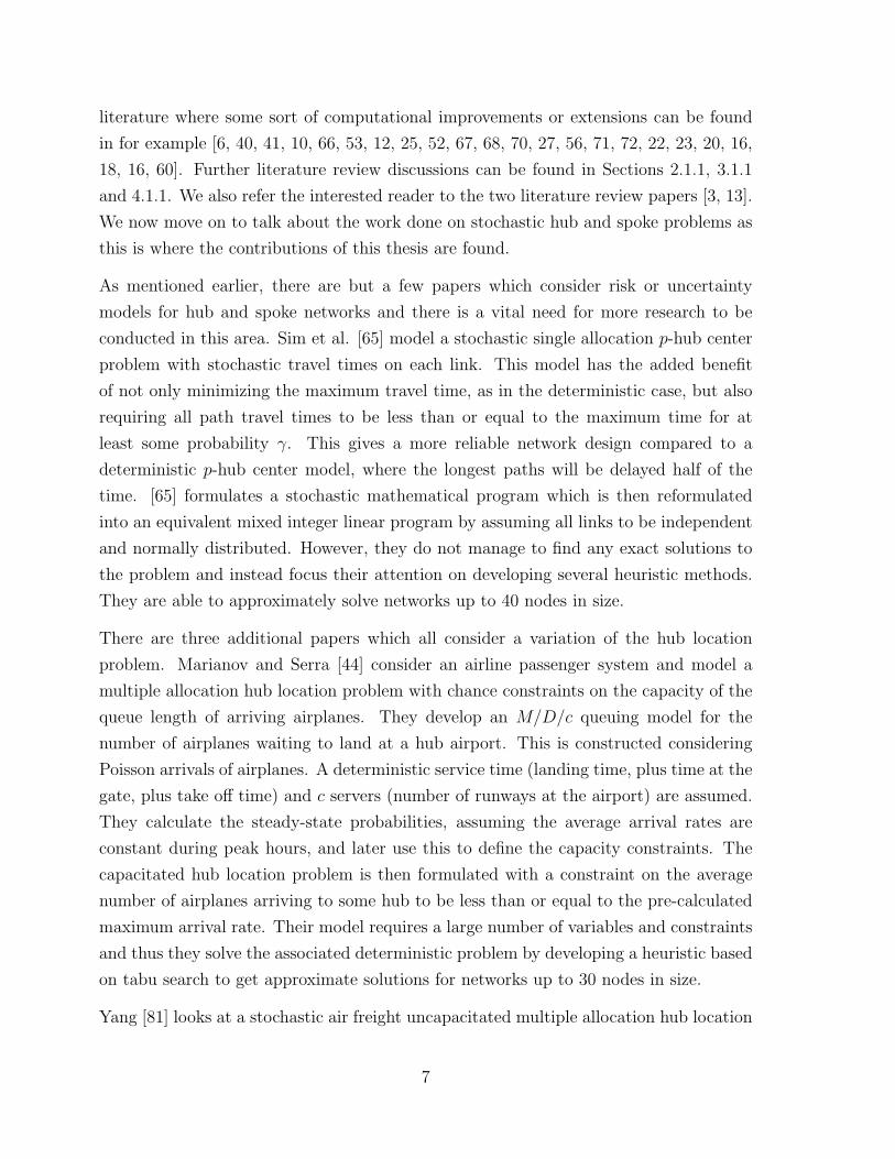
As mentioned earlier, there are but a few papers which consider risk or uncertainty
models for hub and spoke networks and there is a vital need for more research to be
conducted in this area. Sim et al. [65] model a stochastic single allocation p-hub center
problem with stochastic travel times on each link. This model has the added benefit
of not only minimizing the maximum travel time, as in the deterministic case, but also
requiring all path travel times to be less than or equal to the maximum time for at
least some probability γ. This gives a more reliable network design compared to a
deterministic p-hub center model, where the longest paths will be delayed half of the
time. [65] formulates a stochastic mathematical program which is then reformulated
into an equivalent mixed integer linear program by assuming all links to be independent
and normally distributed. However, they do not manage to find any exact solutions to
the problem and instead focus their attention on developing several heuristic methods.
They are able to approximately solve networks up to 40 nodes in size.
There are three additional papers which all consider a variation of the hub location
problem. Marianov and Serra [44] consider an airline passenger system and model a
multiple allocation hub location problem with chance constraints on the capacity of the
queue length of arriving airplanes. They develop an M/D/c queuing model for the
number of airplanes waiting to land at a hub airport. This is constructed considering
Poisson arrivals of airplanes. A deterministic service time (landing time, plus time at the
gate, plus take off time) and c servers (number of runways at the airport) are assumed.
They calculate the steady-state probabilities, assuming the average arrival rates are
constant during peak hours, and later use this to define the capacity constraints. The
capacitated hub location problem is then formulated with a constraint on the average
number of airplanes arriving to some hub to be less than or equal to the pre-calculated
maximum arrival rate. Their model requires a large number of variables and constraints
and thus they solve the associated deterministic problem by developing a heuristic based
on tabu search to get approximate solutions for networks up to 30 nodes in size.
Yang [81] looks at a stochastic air freight uncapacitated multiple allocation hub location
7

problem (UMAHLP) where seasonal variations on demand, as well as seasonal variations
on the discount factors for hub to hub flights, are accounted for. The model is separated
into two stages. The first stage determines the number and location of hubs, taking
into account the solution found from the second stage flight routing problem, where
stochasticity of the seasonal demands and discount factors appear. They rewrite the
two stage model as an extensive form, combining both stages into the same problem to
allow exact solutions to be found. All scenarios from the second stage are accounted for
in the extensive form. They assume a discrete probability distribution, involving three
possible scenarios representing average values for each of the three seasonal variations.
The paper includes and solves a case study of a 10 node air freight network in Taiwan
and China.
Contreras et al. [15] also study a stochastic uncapacitated multiple allocation hub lo-
cation problem. They look at three different cases. First they consider a stochastic
UMAHLP where demand is stochastic. They show that in such circumstances the
stochastic model is equivalent to the deterministic problem where demand is consid-
ered on an average basis, i.e. there is no flaw of averages. Second they consider a
different stochastic UMAHLP where transportation costs on all paths are stochastic,
but assume the costs are all dependent on a single random parameter. They also show
here, as in the first case, that the stochastic model is equivalent to the deterministic
problem, where costs are based on average values. In the third case they similarly ac-
count for stochastic transportation costs on all paths, but now assume all path costs are
independent and described by some known probability distributions. They construct a
Monte-Carlo simulation, using a sample average approximation method coupled with a
Benders’ decomposition algorithm, as a solution approach for the later problem. They
are able to approximately solve the third case model for networks of up to 50 nodes in
size.
There are a lot of existing gaps, both computational and methodological, in the stochas-
tic hub and spoke literature. For example, no existing models consider what percent
of packages actually arrive on time, or account for daily flow volume variations from
different origin nodes and the problems this may cause when capacity constraints exist.
Filling some of these major gaps, like the two just mentioned and more, is the main
contribution of this thesis, to further develop stochastic hub and spoke optimization
models and methods. More research is still however needed and is discussed further in
the conclusion, Chapter 5.
8
Although the location and allocation problem is the topic of this thesis, it is still worth
quickly mentioning some of the other design aspects considered in a working hub and
spoke system. Transportation networks may optimize the unloading, sorting and loading
operations at a hub node. This is of special importance for sea freight terminals where
large volumes of containers are gathered at each port [73]. For truck to truck or truck
to train or airplane (or vice versa) transfers, the cross docking problem is an important
design strategy. The purpose with a cross docking terminal is to unload, sort and load
cargo from different sources onto waiting outbound vehicles. Well planned assignment
of trucks to docks is the key aspect to achieving less costly and fast transfers. Incoming
trucks can be assigned directly to a docking station or asked to wait in a queuing
area until an appropriate docking station is freed up. The queuing system is often
unavoidable, due to trucks generally outnumbering the number of docking stations and
the arrival of a high number of trucks at the same time during peak periods. Due to
the growing number of shipments on a global scale, a common scenario nowadays is
the large queue times of waiting trucks. Many cross docking models are set up slightly
differently with different assumptions, due to the fact that there are very many different
types of docking stations, for example in [82] there are 32 models proposed. However,
papers such as [8, 51] propose a more standard base case model. Similarly, work is also
done for flight gate assignment problems where one of the more common objectives is to
minimize the walking distance of connecting passengers (or sometimes goods) from one
flight to the next [21]. In addition, some hub and spoke networks also need to consider
the vehicle routing problem. The vehicle routing problem optimizes the delivery and
pick up of, for example, mail and cargo from the local buildings which are associated
with each of the individual origin and destination nodes. The vehicle routing problem
can also be found in many other applications outside of hub and spoke networks [31].
9
Chapter 2
Paper One
Exact Computational Approaches to a StochasticUncapacitated Single Allocation p-Hub Center
Problem
Edward Hult, Houyuan Jiang, Daniel Ralph
Judge Business School, University of Cambridge, Trumpington Street, Cambridge CB2 1AG,
United Kingdom, {e.hult,h.jiang,[email protected]}
Abstract
The stochastic uncapacitated single allocation p-hub center problem is an extension of
the deterministic version which aims to minimize the longest origin-destination path in
a hub and spoke network. Considering the stochastic nature of travel times on links is
important when designing a network to guarantee the quality of service measured by a
maximum delivery time for a proportion of all deliveries. We propose an efficient refor-
mulation for a stochastic p-hub center problem and develop exact solution approaches
based on preprocessing and a separation algorithm. We report numerical results to
show effectiveness of our new reformulations and approaches by finding global solutions
of small-medium sized problems.
10

Keywords: Hub location; Center problem; Stochastic programming; Separation algo-
rithm.
2.1 Introduction
Transportation of goods and people plays a vital role in the economy. One of the key
elements affecting the efficiency of shipping services is the network structure. Hub and
spoke networks are often employed to balance cost of building and maintaining services
between pairs of nodes and having short routes, in terms of distance or time, between
pairs of nodes. The hub and spoke structure has found wide application, in air and rail
transportation, postal mail systems, and telecommunication networks [3, 13].
Although traffic flows are patently uncertain, with stochastic travel time on links and
stochastic volumes between nodes to name just two sources of uncertainty, the main
work in the design of hub and spoke networks has focussed on deterministic hub location
models. In this literature stochastic data are replaced by averages. This may be sensible
in some cases but can suggest network designs that are far from optimal, on average, in
a stochastic environment. This phenomenon has been recognized in the facility location
literature [7, 76] and is an instance of a more general notion, the so-called flaw of
averages [62] which merely says that knowing the average values of stochastic inputs to
a process is not enough to determine its average output.
The benefit of deterministic network design is the relative tractability of this problem.
The deterministic model underlying our work is the so-called p-center problem which,
given a list of N nodes and number p less than N , is to identify p nodes as hubs in order to
minimize the maximum travel time across the network. Although this is a combinatorial
optimization problem, progress has been impressive. For instance the work of Meyer et
al. [48] shows that combining clever integer linear programming reformulations with
hybrid algorithms, in a branch and bound framework, can achieve global optimality in
reasonable time for networks of up to 400 nodes.
We consider a stochastic version of the uncapacitated single allocation p-hub center
problem which is the same problem proposed by Sim et al. [65]. The challenge is the
computational burden of dealing with the stochastic problem since it is not obvious how
11

to take advantage of the formulations and methods that are efficient for deterministic
problems. For instance in [65], exact solution seems to be out of the question and even
heuristic methods are at their limits when N = 50. We approach the goal of finding
global solutions in reasonable time in three steps. First we formulate a stochastic model
with chance constraints, second we develop a compact integer linear program (ILP)
reformulation of the stochastic model under certain conditions, and thirdly we adopt
and manipulate various methods and techniques such as preprocessing and introduce a
separation algorithm to find efficient solution procedures.
Beyond exact solutions, exact methods can provide some guarantees on approximation.
For example, an exact solution method based on branch & bound gives guaranteed upper
and lower bounds during execution, even if you stop before an exact solution is found.
However, heuristic methods, even when they identify feasible points, typically are not
associated with guarantees on the quality of such points. The quality of the solution
identified by a heuristic is typically only estimated by extension of empirical results
on problems for which the exact solutions are known. This is not to say heuristics
are not useful: they play an important role and are very powerful for solving large
complicated life sized problems which exact solution methods fail to solve in reasonable
time. However, our main contribution is being able to efficiently solve 40 and 50 node
networks exactly. This is computationally similar to, or better than, the performance of
the heuristic methods proposed in [65] which solve 40 node networks.
Although our stochastic model is similar to that in [65], our reformulation is an ILP using
O(N2) binary variables and O(N3) constraints (see Proposition 2.2.1). This formulation
is compact relative to the reformulation model of [65] (as can be found in the Appendix)
which has O(N4) constraints and O(N4) binary variables. Nevertheless computational
efficiency benefits considerably from preprocessing and separation algorithm approaches.
Indeed the building blocks of our approach — compact ILP reformulations and hybrids
of branch and bound with higher level algorithms — are standard; our contribution is
in part the development of a new reformulation but mainly to demonstrate the value of
exploring generic ILP tools in the stochastic case.
The paper is organised as follows. We review the hub and spoke literature in Section
2.1.1. In Section 2.2 we present the stochastic p-hub center problem (SpHCP) and
establish our compact integer linear programming reformulation (SpHCPL). In Section
2.3, we propose pull (preprocessing) and push (separation algorithm) methods for solving
the ILP reformulation exactly. In Section 2.4, we report numerical results in which exact
12
solution of the stochastic p-hub problem for up to N = 50 is routine.
2.1.1 Literature review
Sim et at. [65] are the first to consider the single allocation p-hub center problem with
stochastic travel times on each link. They formulate a stochastic mathematical program
and then reformulate the problem into an integer linear program by assuming travel time
on links have independent normal distributions. Since exact solutions to this problem
are hard to get the authors focus their attention on developing several heuristic methods
to approximately solve network sizes up to 40 nodes.
In addition to [65] we mention three other hub and spoke papers considering stochas-
tic properties. Marianov and Serra [44] consider a hub location problem with chance
constraints where the arrival times of incoming aircraft are stochastic. They build an
M/D/c queuing model which considers the number of airplanes waiting to land based
on an assumed Poisson arrival rate of the aircraft. The result from the M/D/c queuing
model is then used as a hard constraint requiring the average number of airplanes, arriv-
ing to some hub, to be less than or equal to the found value. They developed a heuristic
algorithm based on tabu search and are able to solve networks up to 30 nodes in size.
Yang [81] looks at an air freight hub location problem where demand and the associated
discount factors on hub-hub links are stochastic. The model is separated into two stages
where the first stage determines the number and location of hubs taking into account
stochasticity that appears in the second stage flight routing problem. [81] assumes a
discrete probability distribution involving only three possible scenarios on demand. The
paper includes a case study of a 10 node air freight network in Taiwan and China. Con-
treras et al. [15] study the uncapacitated multiple allocation hub location problem and
include stochastic properties of both demand and transportation cost. For the rather
special case in which a single random parameter affects the transportation cost on all
links equally, they show that their stochastic model is equivalent to the deterministic
problem in which all random variables are replaced by their average values, i.e., there
is no flaw of averages. For independent transportation costs, however, where the uncer-
tainty of a link cost is independent of all other links in the network, the same cannot
be done. They therefore move on to approximately solve the latter problem for network
sizes up to 50 nodes using Monte-Carlo simulation coupled with Benders’ decomposition.
Although the literature on stochastic hub and spoke networks is small, there is a rel-
13
atively larger pool of research done on deterministic problems. Hub location became
a recognised field of study in the late 1980s. The state-of-the-art for the research in
hub location can be found in two review papers [3, 13]. Attention has focussed on
two themes: proposing mathematical models such as median, center and covering hub
problems to approximate the real-world business challenges, and developing efficient
numerical approaches for solving these proposed mathematical models. Computational
methods dominate the hub location literature. Unsurprisingly, as the number of nodes
in the network grows, exact methods are more prone to computational difficulties —
such as excessive time or memory requirements — than are heuristics.
Campbell [10] is the first to introduce and study the p-hub center problem in the hub
literature. This includes the deterministic version of the problem we study which is
motivated by a hub system involving perishable or time sensitive items in which cost
refers to time.
Campbell [10] defines the uncapacitated single allocation p-hub center problem
(USApHCP) as a quadratic programming problem and proposes a linear programming
reformulation using O(N4) variables where, as above, N is the number of nodes in the
network. The same problem has been studied by several different authors aiming to
speed up the computational efficiency. Kara and Tansel [37] present an equivalent re-
formulation using O(N2) variables and O(N3) constraints. An additional improvement
on the computational performance of the USApHCP was found by Ernst et al. [24] by
reformulating it using what they call the radius approach, which requires only O(N2)
variables and O(N2) constraints. The radius approach can solve test problems that have
up to 200 nodes in the network. Recently a new 2-phase method combining a branch
and bound algorithm and the radius approach was introduced by Meyer et al. [48] and
can solve test examples that have up to 400 nodes. Jutte et al. [36] give a polyhedral
analysis on the hub center problem based on the radius approach.
The other two standard problems in the hub literature are the p-hub median prob-
lem and the hub covering problem which both follow the same trend with different
researchers trying to either improve on the original formulation computationally or to
study extensions and/or variations to the problem. The p-hub median problem, which
is to minimize the total cost of all flows between all OD pairs over the network, has
received more attention in the literature. Transportation costs between hub nodes are
usually discounted by a factor to reflect economies of scale. O’Kelly [49] is the first to
formulate a hub location problem mathematically. Campbell [9, 10] later produces the
14

first integer linear programming formulations for single and multiple allocation p-hub
median problems. Skorin-Kapov et al. [67] reformulate the linear formulation to produce
exact solutions in quicker times. Ernst and Krishnamoorthy [25] present a very efficient
reformulation requires O(N3) variables and O(N3) constraints. Recent advances for the
hub median problems can be found in [16, 60].
The third standard problem is the hub covering problem, first mathematically formulated
by Campbell [10]. The motivation is to find a set of hubs so that the cost of opening
hubs or the number of hubs to use is minimized subject to delivering a certain service.
We refer the interested reader to Alumur and Kara [3] for additional details on hub
covering.
2.2 The Stochastic Hub Center Problem and a Re-
formulation
Here we present the stochastic p-hub center problem (SpHCP for short) after Sim et
al. [65] and, in the deterministic case, Campbell [10]. This is a quadratic program
which has O(N2) binary variables and O(N4) constraints. In Proposition 2.2.1 we show
it has an integer linear program representation of O(N2) binary variables and O(N3)
constraints.
Consider a network consisting of N nodes, denoted by N and options to link any pair
of nodes. The designer wants to select p hubs in N and to assign each node in Nto exactly one hub. If k and m are hub nodes and nodes i and j are allocated to k
and m, respectively, then the path for delivering the goods from node i to node j is
i→ k → m→ j. Assume that Dij represents random travel time between nodes i and j
with an average travel time of dij and a standard deviation of σij. Assume α ∈ (0, 1) is
the discount factor for travel times over hub arcs (links between hub nodes). The total
travel time along the path i→ k → m→ j is Tijkm = Dik + αDkm +Dmj.
Let β be the nominal maximum travel times between all OD pairs in the network.
Assume γ ∈ [0, 1] is the service level. Then the service level guarantee means that for
any nodes i and j, with probability of γ, the travel time for the goods delivered from i
to j will not exceed β. For instance if β = 24 hours and γ = 0.95, then the service level
guarantee requires that the travel time from i to j will not exceed 24 hours for 95% of
journeys. This type of service level guarantee is often employed in call centers and other
15
telecommunication services [30, 32]. Clearly, the designer prefers a smaller value for β
and a larger value for γ. However, these two parameters usually act against each other.
For example, a large value of γ often results in a relatively large value of β.
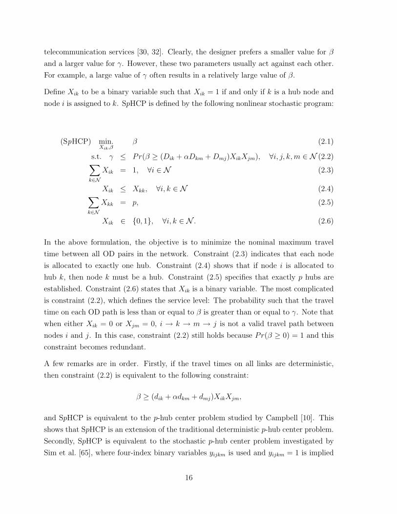
Define Xik to be a binary variable such that Xik = 1 if and only if k is a hub node and
node i is assigned to k. SpHCP is defined by the following nonlinear stochastic program:
(SpHCP) min.Xik,β
β (2.1)
s.t. γ ≤ Pr(β ≥ (Dik + αDkm +Dmj)XikXjm), ∀i, j, k,m ∈ N (2.2)∑k∈N
Xik = 1, ∀i ∈ N (2.3)
Xik ≤ Xkk, ∀i, k ∈ N (2.4)∑k∈N
Xkk = p, (2.5)
Xik ∈ {0, 1}, ∀i, k ∈ N . (2.6)
In the above formulation, the objective is to minimize the nominal maximum travel
time between all OD pairs in the network. Constraint (2.3) indicates that each node
is allocated to exactly one hub. Constraint (2.4) shows that if node i is allocated to
hub k, then node k must be a hub. Constraint (2.5) specifies that exactly p hubs are
established. Constraint (2.6) states that Xik is a binary variable. The most complicated
is constraint (2.2), which defines the service level: The probability such that the travel
time on each OD path is less than or equal to β is greater than or equal to γ. Note that
when either Xik = 0 or Xjm = 0, i → k → m → j is not a valid travel path between
nodes i and j. In this case, constraint (2.2) still holds because Pr(β ≥ 0) = 1 and this
constraint becomes redundant.
A few remarks are in order. Firstly, if the travel times on all links are deterministic,
then constraint (2.2) is equivalent to the following constraint:
β ≥ (dik + αdkm + dmj)XikXjm,
and SpHCP is equivalent to the p-hub center problem studied by Campbell [10]. This
shows that SpHCP is an extension of the traditional deterministic p-hub center problem.
Secondly, SpHCP is equivalent to the stochastic p-hub center problem investigated by
Sim et al. [65], where four-index binary variables yijkm is used and yijkm = 1 is implied
16

by Xik = Xjm = 1.
It is easy to define and understand SpHCP. Also, up to this point, we have not needed
specific assumptions on either the probability distribution of link travel times Dik, or
on the relationship between these random travel times for different links. However, this
formulation involves both integer variables and the stochastic constraint (2.2). These
features make the above formulation computationally intractable. In the sequel, we aim
to convert the above formulation into a computationally tractable deterministic integer
linear program based on two techniques: linearizing quadratic terms, and replacing
probabilistic expressions by equivalent deterministic counterparts. To this end, we make
one more assumption which states that, first, Dij is normally distributed and, second, is
mutually and stochastically independent of Dk` for any nodes i, j, k, ` with (i, j) 6= (k, `).
Based on this assumption, the total travel time Tijkm = Dik+αDkm+Dmj along the path
i → k → m → j is also normally distributed with a mean of tijkm = dik + αdkm + dmj
and a standard deviation of δijkm =√
(σik)2 + α2(σkm)2 + (σmj)2.
The fact that Tijkm has a normal distribution shows that the stochastic constraint (2.2)
is equivalent to a deterministic and quadratic constraint:
β ≥ (tijkm + zγδijkm)XikXjm, ∀i, j, k,m ∈ N ,
where zγ is the z-value for a standard normal distribution and satisfies the equation
Pr(Z ≤ zγ) = γ and Z is a standard normally distributed random variable. Now we can
apply some standard tricks for reformulating a quadratic inequality as a linear inequality.
Evidently, the optimal value for β is nonnegative. Because Xik is a binary variable, it is
easy to verify that constraints β ≥ (tijkm + zγδijkm)XikXjm for all i, j, k,m ∈ N can be
collectively replaced by constraints:
β ≥ (tijkm + zγδijkm)(Xik +Xjm − 1), ∀i, j, k,m ∈ N .
Furthermore, constraint β ≥ (tijkm + zγδijkm)XikXjm or constraint β ≥ (tijkm +
zγδijkm)(Xik +Xjm− 1) is redundant if either Xik = 0 or Xjm = 0. In view of constraint
(2.3), for any fixed i, j,m, constraints β ≥ (tijkm + zγδijkm)(Xik +Xjm − 1) for all k are
equivalent to a single constraint
β ≥∑k∈N
(tijkm + zγδijkm)(Xik +Xjm − 1), ∀i, j,m ∈ N . (2.7)
17

By the above two reformulation techniques, we have obtained an equivalent deterministic
integer linear program for the SpHCP.
Proposition 2.2.1 Assume that for all i, j ∈ N , Dij are mutually and stochastically
independent and normally distributed. Then the stochastic optimization problem SpHCP
defined by (2.1)-(2.6) is equivalent to the following integer linear program:
(SpHCPL) min.Xik,β
β
s.t. (2.3), (2.4), (2.5), (2.6), (2.7).
Having introducing SpHCP and its deterministic counterpart SpHCPL, we make three
remarks in addition to the two made earlier in this section. First, Sim et al. [65] de-
rive a deterministic counterpart from their stochastic optimization problem and the
deterministic counterpart is also an integer linear program. However, the determin-
istic formulation in Sim et al. [65] has 2N4 + N2 + N + 1 constraints and N4 + N2
binary variables, whereas our SpHCPL has only N3 + N2 + N + 1 constraints and N2
binary variables. This seems computationally more promising in terms of both computer
memory and CPU times. Second, the appendix of [65] gives an alternative ILP represen-
tation, with O(N2) variables and O(N4) constraints, requiring an extra assumption on
the stochastic variables, a kind of stochastic triangle inequality. Third, when random-
ness of travel times is removed, SpHCPL is similar to the integer linear programming
formulation studied in Kara and Tansel [37]. The only difference is in the constraint
(2.7) for defining the lower bound β on the objective function, which in [37] is given by
β ≥∑
k∈N (dik + αdkm)Xik + dmjXjm, for each i, j and m in N .
It is important to note that the same approach can be applied for any distribution of
the travel time between nodes provided that the percentiles TDijkm are known in advance,
where TDijkm satisfies the equation Pr(Dij + αDkm + Dmj ≤ TDijkm) = γ. If, unlike the
normal distribution, these percentiles cannot be computed directly, then they can be
found by sampling or simulation techniques which can be carried out independently
from and prior to solving SpHCPL.
18
2.3 Solution Methods
Looking ahead to Section 2.4, our preliminary computational experience in applying
CPLEX to SpHCPL indicates that this combination of model and software is adequate
for problems up of to 25 nodes (Table 2.1). However N = 25 is small for the standard
dataset of test problems, the Australian Post (AP) [26], where deterministic problems of
hundreds of nodes can be solved exactly [48], reasonably quickly. Therefore, in the follow-
ing two subsections, we investigate two computational approaches for solving SpHCPL
more efficiently. These are called pull and push approaches, respectively.
In the pull approach, we aim to remove redundant constraints related to (2.7) and to
add some valid cuts. The push approach is a separation algorithm in which we start
with no or a few constraints of type (2.7) and we gradually add more such constraints if
required. It is worthwhile to mention that Camargo et al. [20] solve the uncapacitated
multiple allocation problem using the Benders’ decomposition approach, which allows
them to solve test examples with a network size of up to 200 nodes.
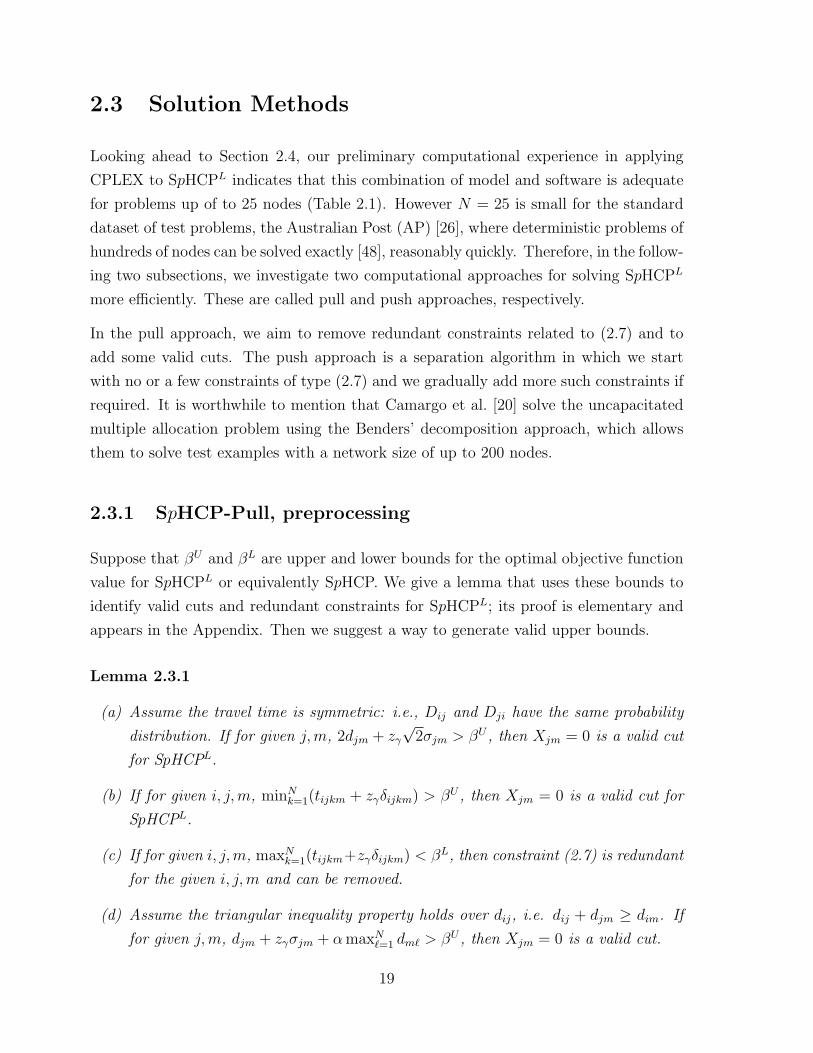
2.3.1 SpHCP-Pull, preprocessing
Suppose that βU and βL are upper and lower bounds for the optimal objective function
value for SpHCPL or equivalently SpHCP. We give a lemma that uses these bounds to
identify valid cuts and redundant constraints for SpHCPL; its proof is elementary and
appears in the Appendix. Then we suggest a way to generate valid upper bounds.
Lemma 2.3.1
(a) Assume the travel time is symmetric: i.e., Dij and Dji have the same probability
distribution. If for given j,m, 2djm + zγ√
2σjm > βU , then Xjm = 0 is a valid cut
for SpHCPL.
(b) If for given i, j,m, minNk=1(tijkm + zγδijkm) > βU , then Xjm = 0 is a valid cut for
SpHCPL.
(c) If for given i, j,m, maxNk=1(tijkm+zγδijkm) < βL, then constraint (2.7) is redundant
for the given i, j,m and can be removed.
(d) Assume the triangular inequality property holds over dij, i.e. dij + djm ≥ dim. If
for given j,m, djm + zγσjm + αmaxN`=1 dm` > βU , then Xjm = 0 is a valid cut.
19
(e) If Xjm = 0 is a valid cut, then for any i and the corresponding j,m, constraint
(2.7) is redundant for SpHCPL.
Based on Lemma 2.3.1, if an upper bound and/or a lower bound for SpHCPL are avail-
able, then we can obtain a better integer linear program than SpHCPL by adding some
additional cuts and by removing some redundant constraints. We call this modified in-
teger linear programming formulation SpHCPL-Pull. The exact format of SpHCPL-Pull
depends on the test example and available upper and lower bounds.
Next we design a heuristic method for deriving an upper bound.
Define d̃ik = dik + zγσik. It is easy to verify that Pr(Dik ≤ d̃ik) = γ, which represents
the service level on the link between i and k. Based on d̃ik, we construct a new network
whose network structure is identical to the existing network, but the direct stochastic
travel time Dik between i and k is replaced by the deterministic travel time d̃ik. For this
new network, we follow Ernst et al. [24] to propose the radius-based formulation:
(Heuristic) min.Xik,rk,β
β
s.t. rk ≥ d̃ikXik,∀i, k ∈ Nβ ≥ rk + rm + αd̃km, ∀k,m ∈ N
(2.3), (2.4), (2.5), (2.6).
Here rk represents the radius of hub node k. When k is not a hub node, rk = 0 holds
automatically. If for all i, k, Dik is a random variable with a single pulse, then Dik =
d̃ik = dik and the above formulation reduces to the radius-based formulation proposed
in Ernst et al. [24]. In terms of computational times, the radius-based formulation is the
state-of-the-art integer linear programming formulation for the single allocation p-hub
center problem. The optimal solution for (Heuristic) gives a feasible solution for SpHCP,
which in turn generates an upper bound for SpHCP.
2.3.2 SpHCP-Push, separation algorithm
In this subsection we focus on the so-called push approach SpHCPL-Push, which is a
separation algorithm. SpHCPL-Push consists of two separate components: so-called
restrictive master problems and, to check their optimality, subproblems. A restrictive
master problem is a modification of SpHCPL by ignoring some constraints of type (2.7).
A subproblem is to check whether or not the most recent restrictive master problem
20

indeed gives an optimal solution to SpHCPL or SpHCP. This can be done by checking
whether or not any constraint of type (2.7) violates if β in (2.7) is replaced by the
optimal objective function value of the most recent restrictive master problem. If not,
an optimal solution for SpHCPL is obtained. Otherwise, such violating constraints are
added to the most recent master problem to form an updated restrictive master problem.
Due to the special structure of SpHCPL, we only need to check constraint violations
for some selected ones of type (2.7). Suppose X∗ik and β∗ are the optimal solution and
the optimal objective function value for the most recent restrictive master problem,
respectively. If X∗jm = 0, then for any i and the corresponding j,m, {X∗ik} satisfies
constraint β∗ ≥∑N
k=1(tijkm + zγδijkm)(X∗ik + X∗jm − 1) automatically, which implies
that there is no need to check constraint violations for any i and the corresponding
j,m. If X∗jm = 1 and constraint β∗ ≥∑
k∈N TDijkmX
∗ik is violated, then for any i and
the corresponding j,m, constraint (2.7) is added to the most recent restrictive master
problem. Note that for any j, there is exactly one m such that X∗jm = 1. Therefore,
we add at most N2 constraints of type (2.7) to the new restrictive master problem.
The above argument also shows that the subproblem can be solved in polynomial time:
checking if Xjm = 0, and checking if β∗ ≥∑N
k=1(tijkm + zγδijkm)X∗ik is violated when
Xjm = 1.
The SpHCPL-Push approach cycles iteratively between restrictive master problems and
subproblems and terminates when an optimal solution for SpHCPL is found. Because
there are exactly N3 constraints of type (2.7) and at least one new and different con-
straint of type (2.7) is added to the restrictive master problem, an optimal solution for
SpHCPL can be found in at most N3 iterations between the restrictive master problem
and the subproblem. The SpHCPL-Push approach as well as some related results is
outlined below.
21
SpHCPL-Push:
Step 1 Generate an initial restrictive master problem: Modifying SpHCPL by removing
all the constraints of type (2.7).
Step 2 Solve the most recent restrictive master problem. Let X∗ik and β∗ be its optimal
solution and optimal objective function value, respectively.
Step 3 Solve the subproblem by checking constraint violations for (2.7) based on the
procedure described above. If there is no constraint violation, terminate and an
optimal solution for SpHCPL is obtained. Otherwise, go to Step 4.
Step 4 Add newly violating constraints to the most recent restrictive master problem
to form a new restrictive master problem. Go to Step 2.
Proposition 2.3.1
(a) The subproblem in SpHCPL-Push is polynomially solvable.
(b) An optimal solution for SpHCPL can be obtained after at most N3 iterations be-
tween the restrictive master problem and the subproblem.
2.4 Numerical Results
In this section, we test the computational performance of the approaches proposed in
the previous sections using well-known test examples from two libraries of test problems,
(CAB) [29, 49] and (AP) [26]. Our code is written in C++, integer linear programs are
solved using ILOG CPLEX Version 12.1, and all of the numerical experiments are carried
out on a HP Pavilion laptop with an Intel(R)Core(TM)2 CPU processor with 3.00 GB
RAM.
The standard CAB and AP test examples are designed for the deterministic p-median
hub location problem. Recall that Dik is assumed to be normally distributed with a
mean of dik and a standard deviation of σik. In our test examples, we assume that dik
takes the value given in the (deterministic) test libraries and σik = νdik, for a constant
ν called the coefficient of variation. In our runs we set ν = 1 and γ = 0.95 for all test
examples and later check the sensitivity of the CPU times with respect to both γ and
ν.
22

We test three approaches: SpHCPL, SpHCPL-Pull, and SpHCPL-Push and let each
run for a maximum of 1 CPU hour (3600 CPU seconds). However, for some of the
smaller test problems which were not solved within the 1 hour time limit, by SpHCPL
or SpHCPL-Pull, a 2 hour time limit was tried but resulted in no additional solutions
found. Note that the problem (Heuristic) introduced in Section 2.3.1 is used for finding
an upper bound for SpHCPL-Pull. Numerical results are shown in the tables below. For
each test problem, we report:
Prob problem name (for CAB examples, a name has a format of N.p.q such that α =
q/10, with the exception of q = 1 then α = q, and for AP examples, a name has a
format of N.p and α = 0.75),
Obj optimal objective function value,
Upper objective function value of the feasible solution generated from (Heuristic) which
provides an upper bound to Obj,
SpHCPL CPU time of running SpHCPL,
SpHCPL-Pull CPU time of running SpHCPL-Pull,
SpHCPL-Push CPU time of running SpHCPL-Push, and
Iter number of iterations for SpHCPL-Push.
For network sizes of 25 nodes or fewer (table 2.1), all methods perform relatively well. In
comparison to the test runs in Sim et al. [65] — where the computational demands of the
ILP formulation of [65] meant that only heuristic approaches could be usefully employed
— our standard SpHCPL formulation appears to be very promising because CPLEX
produces globally optimal solutions for all problems within a few minutes. Moreover,
the difference between SpHCPL-Pull and SpHCPL-Push is very small for network sizes
of 25 nodes or fewer as can be seen in tables 2.1 and 2.2.
For network sizes of 40 nodes or more (table 2.2), however, we can no longer solve
the test problems using SpHCPL with one exception, 40.2, or solve networks of size 50
nodes using SpHCPL-Pull within 1 CPU hour. What is interesting is that SpHCPL-Push
performs very well for the test examples with 40 or 50 nodes.
23
Prob γ ν Obj SpHCPL SpHCPL-Pull SpHCPL-Push Upper Iter
5.3.1 0.95 1 2078.44 0.08 0.02 0.02 2276.84 2
5.3.6 0.95 1 1736.03 0.08 0.02 0.04 1788.54 2
10.2.1 0.95 1 3937.62 0.61 0.13 0.04 3986.21 2
10.2.2 0.95 1 2896.63 0.59 0.08 0.05 2896.63 2
10.2.4 0.95 1 3207.72 0.6 0.17 0.21 3207.72 3
10.2.6 0.95 1 3576.5 0.76 0.16 0.14 3811.55 3
10.2.8 0.95 1 3811.55 0.92 0.07 0.06 3811.55 2
10.3.1 0.95 1 3829.18 0.66 0.06 0.05 3881.41 2
10.3.2 0.95 1 2425.73 0.44 0.05 0.04 2425.73 2
10.3.4 0.95 1 2425.73 0.47 0.05 0.04 2425.73 2
10.3.6 0.95 1 2807.9 0.37 0.05 0.04 2807.9 2
10.3.8 0.95 1 3361.34 0.49 0.05 0.04 3386.14 2
10.4.1 0.95 1 3829.18 0.4 0.21 0.25 4676.7 4
10.4.2 0.95 1 1707.95 0.45 0.06 0.04 1707.95 2
10.4.4 0.95 1 1921.89 0.41 0.03 0.03 1921.89 2
10.4.6 0.95 1 2800.5 0.4 0.04 0.06 2806.02 3
10.4.8 0.95 1 3361.34 0.38 0.06 0.09 3741.36 3
15.2.1 0.95 1 5420.99 3.31 0.69 0.35 5655.94 4
15.2.2 0.95 1 4126.04 2.07 0.54 0.57 4126.04 5
15.2.4 0.95 1 4430.18 2.45 0.66 0.53 4681.75 5
15.2.6 0.95 1 4785.7 2.11 0.45 0.24 4798.08 3
15.2.8 0.95 1 5184.13 2.3 0.45 0.16 5257.06 3
15.3.1 0.95 1 5092.54 2.49 1.44 1.58 6890.21 7
15.3.2 0.95 1 3647.14 1.98 0.26 0.18 3789.68 3
15.3.4 0.95 1 3813.75 2.54 0.53 0.36 3813.75 4
15.3.6 0.95 1 4009.01 2.35 0.14 0.08 4009.01 2
15.3.8 0.95 1 4702.49 2.3 1.1 0.28 5512.17 4
15.4.1 0.95 1 5092.54 1.72 1.39 1.6 6890.21 7
15.4.2 0.95 1 2782.98 1.72 0.25 0.08 2782.98 2
15.4.4 0.95 1 2949.82 2.71 0.13 0.06 2949.82 2
15.4.6 0.95 1 4009.01 3.28 0.41 0.2 4134.12 3
15.4.8 0.95 1 4702.49 2.72 0.69 0.31 5512.17 4
20.2.1 0.95 1 5420.99 13.92 2.55 0.84 5655.94 5
20.2.2 0.95 1 4101.59 9.57 1.14 0.14 4101.59 2
20.2.4 0.95 1 4284.84 9.86 2.25 1.29 4681.75 5
20.2.6 0.95 1 4785.7 9.62 2.07 0.74 4928.59 4
24
20.2.8 0.95 1 5089.27 13.36 2.6 0.81 5420.99 5
20.3.1 0.95 1 5092.54 14.74 9.07 4.04 6890.21 8
20.3.2 0.95 1 3075.01 6.11 0.85 0.14 3075.01 2
20.3.4 0.95 1 3688.54 8.04 2.32 0.8 3813.75 4
20.3.6 0.95 1 4004.81 21.09 0.49 0.11 4032.51 2
20.3.8 0.95 1 4671.23 28.1 6.46 0.69 5171.19 4
20.4.1 0.95 1 5092.54 14.65 6.46 6.77 6890.21 8
20.4.2 0.95 1 2830.12 16.17 1.3 0.44 2922.82 3
20.4.4 0.95 1 3028.72 12.47 0.77 0.2 3028.72 2
20.4.6 0.95 1 4001.28 19.58 0.77 0.33 4060.07 3
20.4.8 0.95 1 4671.23 16.15 5.06 1.26 5406.61 5
25.2.1 0.95 1 5629.69 100.35 1.52 0.19 5646.17 2
25.2.2 0.95 1 4517.81 33.71 6.95 1.61 4617.72 5
25.2.4 0.95 1 4814.33 26.98 10.32 6.18 4895.53 7
25.2.6 0.95 1 5117.46 32.42 2.43 0.63 5117.46 4
25.2.8 0.95 1 5362.94 110.05 1.98 0.21 5362.94 2
25.3.1 0.95 1 5455.94 148.55 3.21 1.22 5982.31 5
25.3.2 0.95 1 3880.84 34.35 5.67 0.89 4105.16 3
25.3.4 0.95 1 4407.47 60.15 15.43 5.66 4439.91 6
25.3.6 0.95 1 4624.12 101.85 4.57 0.36 4624.12 2
25.3.8 0.95 1 5048.59 92.58 0.84 0.14 5060.09 2
25.4.1 0.95 1 5455.94 119.88 18.55 5.96 6911.02 7
25.4.2 0.95 1 3216.94 56.39 2.46 0.71 3216.94 3
25.4.4 0.95 1 3813.75 96.97 2.34 0.5 3813.75 3
25.4.6 0.95 1 4449.14 192.99 14.59 3.3 4617.72 6
25.4.8 0.95 1 5048.59 109.1 5.16 0.87 5342.62 4
Table 2.1: Numerical results for SpHCPL, SpHCPL-Pull, and
SpHCPL-Push, CAB examples.
25

Prob γ ν Obj SpHCPL SpHCPL-Pull SpHCPL-Push Upper Iter
5.2 0.95 1 60402 0.08 0.02 0.05 61525.2 3
5.3 0.95 1 60402 0.07 0.03 0.06 65123.5 3
10.2 0.95 1 87498.2 0.69 0.11 0.04 87498.2 2
10.3 0.95 1 73634.5 0.69 0.1 0.09 75413.2 3
10.4 0.95 1 70902.5 0.53 0.04 0.04 70902.5 2
10.5 0.95 1 70902.5 0.33 0.09 0.15 75086.6 3
20.2 0.95 1 99570.1 8.3 3.13 0.24 99570.1 3
20.3 0.95 1 93111.2 17.91 0.97 0.25 94036.9 3
20.4 0.95 1 90871.9 13.23 2.65 1.75 100351 5
20.5 0.95 1 90871.9 16.5 2.54 1.23 100351 5
20.10 0.95 1 90871.9 4.74 2.47 1.47 100351 5
25.2 0.95 1 114205 51.99 6.2 0.63 115289 3
25.3 0.95 1 109781 53.8 30.53 7.44 120714 6
25.4 0.95 1 109781 30.97 9.17 6.08 120714 7
25.5 0.95 1 109781 37.74 12.36 6.75 120714 7
25.10 0.95 1 109781 16.27 8.86 7.42 120714 14
40.2 0.95 1 131626 1904.91 58.54 2.41 133652 3
40.3 0.95 1 121203 * 278.7 19.19 126088 6
40.4 0.95 1 114571 * 901.98 107.36 131814 7
40.5 0.95 1 114571 * 85.27 125.44 131814 9
40.10 0.95 1 114571 * 150.62 253.41 131814 9
50.2 0.95 1 133722 * * 196.88 141971 6
50.3 0.95 1 120783 * * 70.16 124513 5
50.4 0.95 1 117921 * * 2651.61 131557 10
50.5 0.95 1 117921 * * 1192.33 134376 11
50.10 0.95 1 117921 * * 739.38 134376 19
Table 2.2: Numerical results for SpHCPL, SpHCPL-Pull, and
SpHCPL-Push, AP examples.
To visualize the relative performance among all three numerical methods, we plot the
ratio of the CPU time for each method against the best CPU time among the three
methods. This relative performance of CPU times is given in figure 2.1, which shows
that SpHCPL-Push is a clear winner. We remark that the graphs are truncated at the
performance ratios of 20 and 80 for the CAB and AP datasets, respectively.
26
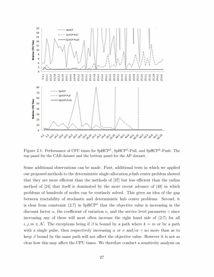
Figure 2.1: Performance of CPU times for SpHCPL, SpHCPL-Pull, and SpHCPL-Push: Thetop panel for the CAB dataset and the bottom panel for the AP dataset.
Some additional observations can be made. First, additional tests in which we applied
our proposed methods to the deterministic single-allocation p-hub center problem showed
that they are more efficient than the methods of [37] but less efficient than the radius
method of [24] that itself is dominated by the more recent advance of [48] in which
problems of hundreds of nodes can be routinely solved. This gives an idea of the gap
between tractability of stochastic and deterministic hub center problems. Second, it
is clear from constraint (2.7) in SpHCPL that the objective value is increasing in the
discount factor α, the coefficient of variation ν, and the service level parameter γ since
increasing any of these will most often increase the right hand side of (2.7) for all
i, j,m ∈ N . The exceptions being if β is bound by a path where k = m or by a path
with a single pulse, then respectively increasing α or ν and/or γ no more than as to
keep β bound by the same path will not affect the objective value. However it is not as
clear how this may affect the CPU times. We therefore conduct a sensitivity analysis on
27

a single test problem, AP 25.2, for a fixed value of γ = 0.95 and ν = 1 respectively. We
check sensitivity of the CPU times of the three methods as functions of ν (γ, resp.) and
observe that the CPU times are not very sensitive to either service level γ or coefficient
of variation ν as can be seen in figure 2.2.
Figure 2.2: Sensitivity results of the CPU times in coefficient of variation ν and service levelparameter γ for test example AP 25.2.
2.5 Conclusion
In this paper we introduce a new formulation (Proposition 2.2.1) for the stochastic unca-
pacitated single allocation p-hub center problem together with two solution procedures
for finding globally optimal solutions based on a preprocessing approach and a separation
algorithm.
The combination of modeling and optimization techniques allows us to solve small to
medium-sized problems in reasonable time. This is in contrast to the original formula-
tion of the problem in Sim et al. [65] where computational difficulties led to the use of
heuristics for even small problems. Of note is the separation algorithm approach where
the subproblem is polynomially solvable, requiring at most N3 iterations. The combi-
nation of the new model formulation and the separation algorithm, we are able to solve
test examples up to 50 nodes in size.
28

Appendix
Proof of Lemma 2.3.1.
(a) Suppose that Xjm = 1. Let j = i and m = k. Then constraint (2.7) reduces to
β ≥ tjjmm + zγδjjmm = 2djm + zγ√
2σjm, which implies that a feasible solution with
Xjm = 1 gives a worse objective function value than the current available upper bound
βU . Hence, Xjm = 0 is a valid cut for SpHCPL.
(b) Suppose that Xjm = 1. Then constraint (2.7) reduces to
N∑k=1
(tijkm + zγδijkm)Xik ≥N
mink=1
(tijkm + zγδijkm)N∑k=1
Xik =N
mink=1
(tijkm + zγδijkm),
which is greater than βU according to the assumption. This shows that any feasible
solution with Xjm = 1 gives a worse objective function value than βU . Therefore,
Xjm = 0 is a valid cut for SpHCPL.
(c) Suppose that Xjm = 1. Then constraint (2.7) reduces to
β ≥N∑k=1
(tijkm+zγδijkm)Xik ≤N
maxk=1
(tijkm+zγδijkm)N∑k=1
Xik =N
maxk=1
(tijkm+zγδijkm) < βL,
which is redundant for the given i, j,m.
(d) Suppose that Xjm = 1 and assume dmi = maxN`=1 dm` and Xin = 1. It follows from
constraint (2.7) and the triangle inequality property that
β ≥ (tijnm + zγδijnm)
= din + αdnm + dmj + zγ√
(σin)2 + α2(σnm)2 + (σmj)2
≥ αdim + dmj + zγσmj
= dmj + αmaxN`=1 dm` + zγσmj
> βU .
This shows that any feasible solution with Xjm = 1 gives a worse objective function
value than βU . Hence Xjm = 0 is a valid cut.
(e) When Xjm = 0, the right-hand side of constraint (2.7) for any i and the corresponding
j,m is non-positive. Clearly, this constraint is redundant for SpHCPL.
29

ILP reformulation in Sim et al. [65]
min.Xik,Yikmj ,β
β
s.t. β ≥ (dik + αkm + dmj + zγ
√σ2ik + α2σ2
km + σ2mj)Yikmj, ∀i, j, k,m ∈ N
Yikmj ≥ Zik + Zjm − 1, ∀i, j, k,m ∈ N∑k∈N
Zik = 1, ∀i ∈ N
Zik ≤ Zkk, ∀i, k ∈ N∑k∈N
Zkk = p
Yikmj ∈ {0, 1}, ∀i, j, k,m ∈ N
Xik ∈ {0, 1}, ∀i, k ∈ N
30
Chapter 3
Paper Two
Service Risk in Hub and Spoke Networks
Edward Hult
Judge Business School, University of Cambridge, Trumpington Street, Cambridge CB2 1AG,
United Kingdom, {[email protected]}
Abstract
The stochastic single allocation p-hub center problem aims to find the shortest service
or delivery time guarantee over all paths in a hub and spoke network. This guarantee is
set to hold for a minimum probability γ. The model considers the important stochastic
nature of travel times on links but, unlike the deterministic single allocation p-hub
center problem, departure times at hub nodes are not accounted for automatically. Not
accounting for departure times may result in a non-optimal solution design for real
life networks. We propose two new methodological approaches, motivated from talks
with a few different European transportation companies, respectively accounting for
variable and fixed departure times at hub nodes. An approximation solution is proposed
for the variable departure times model using a step function where we prove that the
optimal location-allocation solutions to the approximation model converge to the optimal
location-allocation solutions of the original stochastic model when the step size is small
31

enough. In addition a linear model is formulated to give exact solutions to the stochastic
p-hub center model with fixed departure times. We also propose a different risk model,
using fixed departure times, which minimizes the penalty cost for origin-destination pairs
missing some given maximum delivery service guarantee. The purpose is to maximize
the volume of packages which arrive on time in contrast to the center problem which is
path based. Three exact solution approaches are also constructed and numerical results
are reported for all new models demonstrating the effectiveness of the respective solution
approaches.
Keywords: Hub location; Center problem; Stochastic programming.
3.1 Introduction
In hub and spoke networks the flow of packages from origin to destination is designed to
be simple and cost efficient. All packages from different origin nodes are collected and
brought, often by truck, to a relatively nearby hub. The packages at the hub are then
sorted and consolidated into bigger delivery vehicles, such as airplanes or trains, for a
quicker and more cost effective transfer to a relatively far off located hub. If the origin-
destination nodes are geographically close this second leg is skipped if both nodes are
connected to the same hub. At the second hub, packages are disaggregated and sorted
for distribution to all the directly connected destination nodes. A typical delivery path
is shown in figure 3.1.
Figure 3.1: Origin-destination path via hub nodes.
Fast delivery times and strong service guarantees are vital aspects for modern day trans-
portation and delivery companies. This paper presents new mathematical modeling
tools, for network managers, providing effective design solutions. An effective solution
provides a design which is practical and provides both fast and reliable delivery time
32

guarantees. The main focus of the paper is on mail and parcel delivery networks but
many of the ideas developed here can be directly applied to any hub and spoke type
network.
The majority of work done on hub and spoke systems in the literature assumes deter-
ministic network properties, for example demand and link travel times are based on
average values. However, assuming fixed travel times on links in a network when con-
sidering delivery times and service guarantees is a very big assumption and can lead to
poor solutions with huge additional costs, see for example Example A in the Appendix.
Strong assumptions are however not uncommon in the mathematical modeling commu-
nity and many researchers and practitioners alike will often make several assumptions
and simplifications when designing models due to the dynamic and highly complicated
properties of real life systems. This paper aims to help bridge the gap between theo-
retically solvable models and practical and useful design solutions for real life mail and
parcel delivery systems.
In our quest to help bridge the theory-practice gap we contacted four European mail
and parcel companies including a major European postal company. We did this to find
out what the industry’s thoughts are on considering stochastic travel times in the design
process of the network. In our talks with the different companies they all emphasized
the importance of having a well structured and well timed network based on stochastic
link travel times. This is because at each hub there is a set departure time, which must
be based on the variations of each link’s travel time, so that incoming units can arrive
on time. In the classic p-hub center problem, first studied by Campbell [10], which
minimizes the maximum delivery time, link travel times, and therefore also departure
times, are based on average values [38, 74]. This creates a problem since any travel time
variation longer than the average on a link will miss the delivery time guarantee or will
delay the departure time at the upcoming hub causing a chain effect delay for multiple
delivery destinations or a missed departure altogether.
Sim et al. [65] and later Hult et al. [33] consider the stochastic nature of travel times
on links and solve the stochastic uncapacitated single allocation p-hub center problem.
They minimize the maximum delivery time β for a guaranteed service level in a network.
The service level is the probability that the travel time on each origin-destination path
is less than or equal to β is greater than the given probability γ. However, for the
delivery path to hold all incoming packages must arrive at each hub before the set
departure time from hub k to hub m and from hub m to destination node j. In the
33
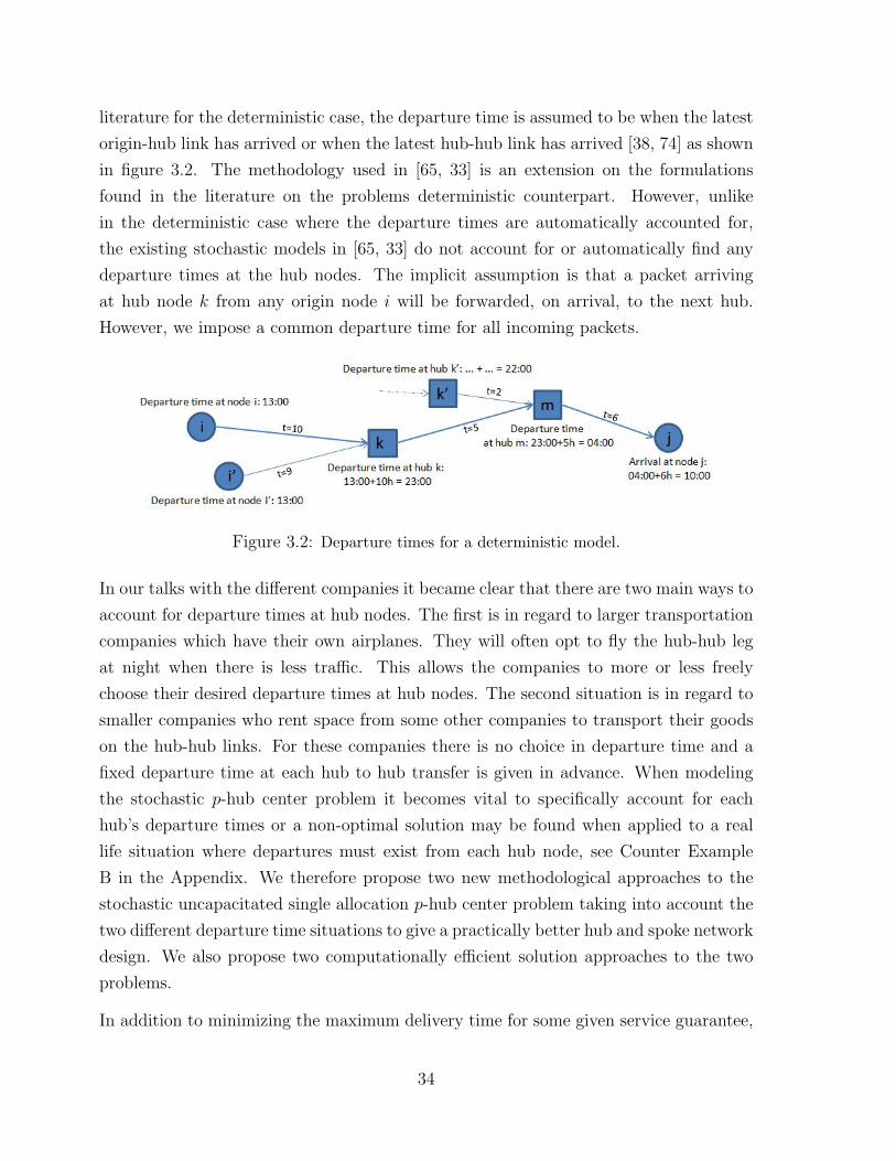
literature for the deterministic case, the departure time is assumed to be when the latest
origin-hub link has arrived or when the latest hub-hub link has arrived [38, 74] as shown
in figure 3.2. The methodology used in [65, 33] is an extension on the formulations
found in the literature on the problems deterministic counterpart. However, unlike
in the deterministic case where the departure times are automatically accounted for,
the existing stochastic models in [65, 33] do not account for or automatically find any
departure times at the hub nodes. The implicit assumption is that a packet arriving
at hub node k from any origin node i will be forwarded, on arrival, to the next hub.
However, we impose a common departure time for all incoming packets.
Figure 3.2: Departure times for a deterministic model.
In our talks with the different companies it became clear that there are two main ways to
account for departure times at hub nodes. The first is in regard to larger transportation
companies which have their own airplanes. They will often opt to fly the hub-hub leg
at night when there is less traffic. This allows the companies to more or less freely
choose their desired departure times at hub nodes. The second situation is in regard to
smaller companies who rent space from some other companies to transport their goods
on the hub-hub links. For these companies there is no choice in departure time and a
fixed departure time at each hub to hub transfer is given in advance. When modeling
the stochastic p-hub center problem it becomes vital to specifically account for each
hub’s departure times or a non-optimal solution may be found when applied to a real
life situation where departures must exist from each hub node, see Counter Example
B in the Appendix. We therefore propose two new methodological approaches to the
stochastic uncapacitated single allocation p-hub center problem taking into account the
two different departure time situations to give a practically better hub and spoke network
design. We also propose two computationally efficient solution approaches to the two
problems.
In addition to minimizing the maximum delivery time for some given service guarantee,
34

as in the stochastic p-hub center problem, it became clear from our talks that companies
are interested in finding a network setup which looks at the percent of packages which
are delivered in time and not just paths which deliver in time. To accommodate this
we propose a new model, with three accompanying solution approaches, which we call
the Service Cost Problem (SCP) and is introduced in Section 3.3. This differs from the
stochastic p-hub center problem by taking into account the volume on paths for a given
delivery time, such as a 24 hour delivery guarantee.
The paper is set up in the following way. A deeper look at the literature is presented
in Section 3.1.1. In Section 3.2 the two new methodological approaches to a stochastic
p-hub center problem are introduced in Sections 3.2.1 and 3.2.2 together with their
respective models and solution procedures. Numerical results are presented in Section
3.2.3. In Section 3.3 the new service cost problem is introduced and formulated in
Section 3.3.1. Solution procedures are presented in 3.3.2 and numerical results given in
Section 3.3.3. The paper ends with a short conclusion in Section 3.4.
3.1.1 Literature review
Hub and spoke research is a relatively new field of research and O’Kelly [49] was the
first to formulate a hub location problem mathematically, named the single allocation
p-hub median problem. Campbell [9] and [10] later produced the first linear integer
programming formulations for the multiple and single allocation p-hub median problems
respectively. The goal here is to minimize the total cost of flow across the network
by finding p number of hub nodes and allocating each additional node to one (single
allocation) or more (multiple allocation) hubs. Additionally Campbell [10] introduced
two other main problems which have become standard in the hub and spoke literature,
the p-hub center problem and the hub covering problem. The p-hub center problem aims
to minimize a defined maximum cost over the links or paths, for example minimizing
the maximum travel time for any origin-destination pair. The hub covering problem is
about finding a set of hubs so that the distances for origin and destination nodes to hub
nodes fulfill a certain criterion. The objective can for example be to minimize the cost of
opening hubs to reach all destinations or to maximize the flow under a set of constraints.
The p-hub median problem has received the most attention in the literature but all three
have been studied with a focus on either improving the computational performance or
creating different model variations to represent more realistic systems.
35

Strong computational improvements on the p-hub median problem were made in Skorin-
Kapov et al. [67] and in Ernst and Krishnamoorthy [25]. Later Camargo et al. [20]
solved the uncapacitated multiple allocation problem using Benders’ decomposition, al-
lowing network sizes of up to 200 nodes to be solved in a few hours. Contreras et al. [16]
solved the capacitated single allocation problem using column generation together with
a Lagrangean relaxation also solving networks up to 200 nodes. Other variations on the
median problem can be found in, for example, Elhedhli and Hu [23] who consider conges-
tion effects at hub nodes, adding a non-linear congestion cost function to the objective of
the uncapacitated single allocation p-hub median problem. Costa et al. [18] remodeled
the capacitated single allocation hub location problem, which itself is a variation of the
p-hub median problem also introduced in [10], by removing the capacity constraints and
instead adding a second objective function to the formulation, minimizing the time a
hub takes to process the incoming flow. Martin and Roman [47] and Sasaki [61] use
one-hub models for capturing competition properties in airline companies. Marianov et
al. [45] studied competition in a hub network aimed to maximize the total captured flow
by using a constraint for the travel cost stating that if the travel cost is not less than a
certain market value between an OD pair, then there will be no flow between that OD
pair.
The p-hub center problem, also first discussed by Campbell [10], aims to minimize the
maximum cost of a defined type of flow over a link or path, for example minimizing the
maximum length of travel for any origin-destination pair. The original formulations of
the uncapacitated single allocation p-hub center problem [10] consisted of a quadratic
programming formulation and also a linear programming formulation using O(n4) vari-
ables. Kara and Tansel [37] later improved on this by formulating the problem using
O(n2) variables and O(n3) constraints. An additional improvement on the computa-
tional performance was found by Ernst et al. [24] by reformulating it using what they
called the radius of hub k resulting in an O(n2) variable and constraint formulation. The
radius of hub k model solves problem sizes consisting of 100 nodes without any major
concerns. Meyer et al. [48] introduced a very efficient 2-phase method which can solve
400 node networks in a relatively short period of time. They use a branch and bound
algorithm to find potential optimal hubs and then solve the allocation problem sepa-
rately for each node in the branch and bound forest. Kara and Tansel [38] modeled the
latest arrival hub location problem taking into the account the departure times at each
hub. However, the departure times at each hub are assumed to be at the time the last
cargo arrives at the hub and this was shown in [74] to be equivalent to the methodology
36
of the original p-hub center problem. Yaman et al. [80] also develop a latest arrival hub
location problem in which they allow stopovers to occur on the node-hub links, such as
when a truck may stop at several nodes on its way to the hub node. They solve network
sizes of up to 16 nodes.
Many variations exist for deterministic hub and spoke problems and the interested reader
is referred to the two literature review papers [3, 13]. As for stochastic hub and spoke
research the literature is much smaller. Marianov and Serra [44] developed a heuristic
algorithm based on tabu search to solve a hub location problem with chance constraints.
They build an M/D/c queuing model which considers the number of airplanes waiting to
land based on an assumed Poisson arrival rate of the aircraft. The result from theM/D/c
queuing model is then used in the chance constraint requiring the average number of
airplanes, arriving to some hub, to be less than or equal to the found value. They are
able to solve networks up to 30 nodes in size. Sim et at. [65] developed a stochastic
version of the single allocation p-hub center problem based on normally distributed link
travel times. They developed several heuristic methods to approximately solve network
sizes up to 40 nodes. Later Hult et al. [33] studied the same problem as [65] but
presented exact solution methods based on preprocessing and a separation algorithm
which are able to solve up to 50 node networks. Yang [81] developed a two stage
model considering stochastic demand and stochastic discount factors on the hub-hub
links for an air freight hub location problem. They consider three possible discrete
scenarios on demand and conduct a case study of a 10 node air freight network in
Taiwan and China. Contreras et al. [15] constructed and solved, using Monte-Carlo
simulation coupled with Benders’ decomposition, a stochastic uncapacitated multiple
allocation hub location problem using stochastic independent transportation costs. They
are able to approximately solve networks up to 50 nodes in size. There is a much
larger pool of research done in the similar but, modeling wise, simpler field of stochastic
facility location problems. The interested reader is referred to the large stochastic facility
location literature review paper [69].
37
3.2 New Methodological Approach to a Stochastic
p-hub Center Problem
Given a network of N nodes denoted by N , the designer wants to find an optimal single
allocation solution for each node in N to a set of p hubs in N so as to minimise the
longest path, β, in the network. β is set such that all deliveries from an origin-destination
pair (OD pair) arrive before the maximum time β for at least a given probability γ. For
each OD pair i → j, shipments are transported via some hub nodes k and m where
k may be equal to m in some cases. We assume all hub nodes to be fully connected.
Define Xik to be a binary variable such that Xik = 1 if and only if node i is allocated to
hub node k.
Assume T 1ik to be the stochastic travel time from node i to hub k plus the time for
unloading, sorting and loading after arrival. Similarly assume T 2mj to be the stochastic
travel time from hub m to node j plus the time from the latest arrival, Am, to hub m
until the actual departure time from m to node j. The random time from the latest
arrival to departure accounts not only for possible random effects of unloading, sorting
and loading times but also accounts for possible randomness in the travel times on
the incoming hub-hub links, although according to the talks we had with the different
companies, the hub-hub links are often very reliable and have low variance. Assume all
T 1ik and all T 2
mj are independent and normally distributed random variables where t1ikand t2mj are the means and σ1
ik and σ2mj are the standard deviations respectively. Define
tkm to be the expected travel time for each hub-hub link and α as the discount factor
associated with the hub to hub transfers. The triangle inequality is assumed to hold for
all mean travel times but not for their respective variances.
To find an optimal solution to the uncapacitated single allocation p-hub center problem
with stochastic travel times we need to incorporate and account for departure times.
Not doing so may lead to non-optimal solutions, as seen in Counter Example B in the
Appendix. In addition a delay in the departure from a hub to hub link can cause a chain
effect delay across the network resulting in several OD pairs missing their guaranteed
delivery times. The departure time for each hub-hub link, k to m, is modelled in
two different ways, depending upon the type of transportation company, and each are
discussed further in the following two sections. The departure time, Am, from hub m to
destination node j, is more flexible, due to the more flexible modes of transportation in
regards to departure times used on the hub-node links. Although it is modelled to depart
38
when the last leg has arrived it allows for delays to account for sorting and loading times
of the goods. The sorting and loading times are captured by the stochastic travel time
T 2mj. In addition we assume that all origin node shipments depart at the same time,
for example at 16:00 from each origin depot. This can however very simply be modified
by adding the constant ti onto T 1ik in all formulations (for example T 1
ikXik turns into
(T 1ik + ti)Xik) which represents a positive or negative number associated with a later or
earlier departure time than the norm for each origin node i respectively.
3.2.1 Variable departure times
Larger delivery companies which have access to their own airplanes, for the hub-hub link
transfers, often opt to fly at night. At night there is less passenger travel and finding
a departure time becomes less about checking what slot times are available and more
about figuring out when will the packages arrive and how long will it take to sort and
load them onto the outbound flights.
To capture this additional question we propose a stochastic p-hub center model which
also solves for an optimal departure time, Dk, from each hub k to all hubs m. We model
the flow through the network in the following way. The packages flow from an origin
node i departing at time “zero”. T 1ik time units later they have arrived and been sorted
and will get loaded to depart from hub k to hub m by time Dk. From k they travel
to hub m taking αtkm time units, where α is the discount factor, associated with the
often faster mode of transportation, for travel times over hub arcs. At hub m they wait
till the time Am for when the last cargo has arrived. Everything then gets loaded onto
outbound trucks from hub m to be delivered to some destination node j which takes T 2mj
time units from Am and arrives before the maximum time β with a minimum probability
γ.
We assume all departures from a hub k can be made simultaneously. This assumption
is the same and in accordance with the literature for the deterministic versions of the
problem and is satisfactory since only the longest path in the network realistically needs
to depart on the found departure time for the delivery service to hold. All other paths
can depart in order of length and will most often not delay the delivery service. The
exception is if two paths are of same length which both make up the longest path in
the network and are routed via the same hub k to go to two different hubs m and m′,
then one will have to wait till the other has departed and may cause the path on the
39

later departing flight to slightly increase β so as to hold with a probability γ. This effect
however is very small given the entire length of the paths and will have a very small
impact on the optimality of the network structure.
The stochastic p-hub center problem with variable departure times (SpHCPDV ) lets
the designer solve for the optimal hub locations and node allocations and the optimal
departure times at each hub while minimizing the nominal maximum travel time for all
OD pairs via the decision variables Xik, Dk, Am and β respectively.
(SpHCPDV )
min.Xik,Dk,Am,β
β (3.1)
s.t. γ ≤ Pr[T 1ikXik ≤ Dk ∩ (Am + T 2
mj)Xjm ≤ β],∀i, j, k,m ∈ N (3.2)
Am ≥ (Dk + αtkm)XkkXmm, ∀k,m ∈ N (3.3)∑k∈N
Xik = 1, ∀i ∈ N (3.4)
Xik ≤ Xkk, ∀i, k ∈ N (3.5)∑k∈N
Xkk = p (3.6)
Xik ∈ {0, 1}, ∀i, k ∈ N (3.7)
Dk ≥ 0, ∀k ∈ N (3.8)
Am ≥ 0, ∀m ∈ N (3.9)
The objective function (3.1) minimizes the maximum travel time β for all paths in the
network. The chance constraints (3.2) state that the probability of a path i− k−m− jto arrive before the time β is greater than or equal to γ. Constraint (3.3) finds the latest
arrival from all incoming hub links to hub m. Constraints (3.4)-(3.7) are standard for
the uncapacitated single allocation p-hub problem and respectively state that all nodes
must be assigned to exactly one hub, a node can only be assigned to a node k if k is a
hub node, exactly p hubs should be found and lastly all Xik are binary.
Going forward we have two objectives. One is to reduce the size of the formulation,
from O(N4) to O(N2) constraints, and the second, to make the chance constraints (3.2)
linear. The goal is to find solutions to midsized problems within reasonable time.
We note that (Dk + αtkm)XkkXmm in (3.3) could be directly inserted into constraint
40
(3.2) since the binding link i− k will always result in the latest arrivals to hub m from
k due to the variable departure time Dk. This allows constraints (3.2) and (3.3) to be
replaced by:
γ ≤ Pr[T 1ikXik ≤ Dk ∩ ((Dk + αtkm)XkkXmm + T 2
mj)Xjm ≤ β], ∀i, j, k,m ∈ N (3.10)
and thus also eliminating the need for the decision variable Am. In addition due to
the independence of the random variables T 1ik and T 2
mj, (3.10) can also be rewritten by
adding the decision variables p1 and p2 using the following set of constraints:
p1 ≤ Pr[T 1ikXik ≤ Dk], ∀i, k ∈ N (3.11)
p2 ≤ Pr[((Dk + αtkm)XkkXmm + T 2mj)Xjm ≤ β], ∀j, k,m ∈ N (3.12)
γ ≤ p1p2 (3.13)
By adding the decision variables rm, (3.12) can be changed to:
p2 ≤ Pr[T 2mjXjm ≤ rm], ∀j,m ∈ N (3.14)
β ≥ Dk + αtkm + rm, ∀k,m ∈ N (3.15)
Constraints (3.14) and (3.15) are equivalent to (3.12) since β in (3.15) must be greater
than or equal to the departure time from hub k plus the travel time from hub k to hub m
plus the longest time required for packages to travel from hub m to some destination node
j whose time is guaranteed to hold for a minimum probability p2 in (3.14). Additionally
if k and/or m are not hub nodes (3.15) will not be binding since, for example, if k is
not a hub then Dk will be zero and k will be allocated to some other hub node k′. This
holds since
β ≥ Dk′ + αtk′m + rm ≥ tkk′ + zp1σkk′ + αtk′m + rm ≥ αtkm + rm
due to the triangle inequality of the mean times and where zp1 is the z-value from the
standard normal distribution table for the probability p1.
This results in an O(|N |2) instead of an O(|N |4) constraint formulation which we call
41
SpHCPDV 2and is equivalent to SpHCPDV .
(SpHCPDV 2
)
min.Xik,Dk,rm,p1,p2,β
β
s.t. rm ≥ 0, ∀m ∈ N (3.16)
p1 ≥ 0 (3.17)
p2 ≥ 0 (3.18)
(3.4), (3.5), (3.6), (3.7), (3.8)
(3.11), (3.13), (3.14), (3.15)
In SpHCPDV 2, Dk and rm also represent the radius of hub k and hub m for collection
and distribution respectively. This is similar to the radius of hub k formulation by Ernst
et al. [24] for the deterministic p-hub center problem, but here with chance constraints.
However, the chance constraints (3.11) and (3.14) will still cause computational prob-
lems. We therefore reformulate SpHCPDV 2into an approximate deterministic linear
formulation using a step function which can be optimally solved. The step function is
in regards to the probability of reaching the different departure times at the different
hubs and destination nodes and is defined by the set L where
L = {(P 1l , P
2l ) ∈ [γ, 1] | P 1
l = γ + lδ, P 1l P
2l = γ, l = 0, . . . , L}
for δL = 1−γ. When |L| → ∞ we will show that the optimal solutions will be the same
since all probability combinations of P 1l and P 2
l will be accounted for and will correspond
with p1 and p2 in SpHCPDV 2. Moreover, the optimal location-allocation solution, X∗ik,
converges with an increasing |L|.
Since the two vectors P 1l and P 2
l have the set L of possible probability combinations we
can pre-calculate the parameters t1ikl and t2mjl so that
P 1l = Pr[T 1
ik ≤ t1ikl] (3.19)
and
P 2l = Pr[T 2
mj ≤ t2mjl] (3.20)
hold. Since T 1ik and T 2
mj are assumed to be normally distributed this can be calculated
42
by setting t1ikl = t1ik + z1l σ
1ik and t2mjl = t2mj + z2
l σ2mj where z1
l and z2l represent the z-
value from the standard normal distribution table for each of the probabilities P 1l and P 2
l
respectively. However, if T 1ik and T 2
mj are not normally distributed t1ikl and t2mjl can easily
be estimated by simulation and/or sampling at this stage for each of their respective
different probabilities in P 1l and P 2
l .
Since γ = P 1l P
2l = Pr[T 1
ik ≤ t1ikl]Pr[T2mj ≤ t2mjl] we can set:∑
l∈L
t1iklXikYl ≤ Dk, ∀i, k ∈ N (3.21)
and ∑l∈L
t2mjlXjmYl ≤ rm, ∀m, j ∈ N (3.22)
where Yl is a binary variable equal to one if the probability combination (P 1l , P
2l ) ∈ L
is chosen and will guarantee that P 1l ≤ Pr[T 1
ikXik ≤ Dk] and P 2l ≤ Pr[T 2
mjXjm ≤ rm]
for the chosen l ∈ L. Note that the same probability combination is chosen for all
outbound and inbound links, since all outbound links are connected to all inbound
links. This allows us to reformulate SpHCPDV 2into an approximate linear formulation
using the decision variables Xik, Yl, Dk, rm and β with a step function consisting of
different probability combinations (P 1l , P
2l ) ∈ L represented by t1ikl and t2mjl.
(SpHCPDVL )
min.Xik,Yl,Dk,rm,β
β
s.t. Dk ≥∑l∈L
t1ikl(Xik + Yl − 1), ∀i, k ∈ N (3.23)
rm ≥∑l∈L
t2mjl(Xjm + Yl − 1), ∀m, j ∈ N (3.24)
1 =∑l∈L
Yl (3.25)
Yl ∈ {0, 1}, ∀l ∈ L (3.26)
(3.4), (3.5), (3.6), (3.7), (3.8), (3.15), (3.16)
Constraints (3.23) and (3.24) are linearizations of (3.21) and (3.22) and calculate the
43

radii of hubs k and m respectively for a chosen l ∈ L. Constraint (3.25) allows only one
probability combination to be chosen and (3.26) is the binary constraint.
We now show that for |L| large enough, the optimal location-allocation solution, Xik,
for SpHCPDVL will also be optimal for SpHCPDV 2
. First off, it is good to note that there
will always exist a feasible and optimal solution to both SpHCPDV 2and SpHCPDV
L , as
long as |N | ≥ p > 0, since Dk, rm and β are decision variables.
Definition 3.2.1 Define F as the set of location-allocation solutions Xik, for all i, k of
(3.4) - (3.7) and denote an arbitrary location-allocation solution by f ∈ F .
It is clear that F has finite cardinality, and is the set of feasible location-allocation
solutions for each of the problems SpHCPDV 2and SpHCPDV
L .
Definition 3.2.2 For each solution f ∈ F there exists an optimal value β, which is the
minimum value of the objective function with respect to minimizing the longest path in
the network, defined as βf and βLf for SpHCPDV 2and SpHCPDV
L , respectively. βf and
βLf are found by minimizing the decision variables Dk, rm, p1, p2 and Dk, rm, Yl for
SpHCPDV 2and SpHCPDV
L , respectively, for each solution f ∈ F .
Lemma 3.2.1 Solving for an optimal βf gives equality of constraint (3.13), γ = p1p2.
Proof: Remembering that T 1ik and T 2
mj are normally distributed, we know that the
cumulative distributions Pr[T 1ik ≤ ζ] and Pr[T 2
mj ≤ ζ] are strictly decreasing for each
i, k ∈ N and m, j ∈ N . With this property in mind, it is clear that if a gap γ < p1p2
exists, reducing the values of the decision variables Dk and rm on the binding constraints
of (3.11) and (3.14), respectively, will remove the gap and give a lower βf value from
(3.15) for any given f ∈ F .
Lemma 3.2.2 βLf → βf as |L| → ∞ ∀f ∈ F .
Proof: Assume D∗k, r∗m, p1∗ and p2∗ are the optimal solutions when solving for βf for
a given f ∈ F denoted by X ′′ik. Also assume DLk , rLm and Y L
l are the optimal solutions
when solving for βLf for the same f ∈ F and assume l′ is the value of index l ∈ L for
when Y Ll′ = 1. From (3.11) we get
p1∗ = mini,k∈N
(Pr[T 1ikX
′′ik ≤ D∗k])
44

and from (3.23) we get
DLk = max
i∈N(t1ikl′X
′′ik) (3.27)
which from (3.19) results in
P 1l′ = Pr[T 1
ik ≤ t1ikl′ ] = mini,k∈N
(Pr[T 1ikX
′′ik ≤ t1ikl′X
′′ik]) = min
i,k∈N(Pr[T 1
ikX′′ik ≤ DL
k ]).
The possible values of DLk , when it is binding as in (3.27), are bound by the possible
choices of l′ ∈ L. However, when |L| → ∞ the possible values of DLk , when binding,
becomes continuous as Dk is in SpHCPDV 2. Therefore when |L| → ∞
| mini,k∈N
(Pr[T 1ikX
′′ik ≤ D∗k])− min
i,k∈N(Pr[T 1
ikX′′ik ≤ DL
k ])| → 0
which gives |D∗k − DLk | → 0 and |p1∗ − P 1
l | → 0. The same steps can be taken using
constraints (3.14), (3.20) and (3.24) to show that |r∗m − rLm| → 0 and |p2∗ − P 2l | → 0.
Therefore from (3.15) we get βLf → βf for any given f ∈ F .
Definition 3.2.3 The set O is a subset of F which represents the optimal location-
allocation solutions for SpHCPDV 2.
Lemma 3.2.3 There exists a positive gap ε such that βf∗ + ε < βf , ∀f ∗ ∈ O and
∀f ∈ F \ O.
Lemma 3.2.3 holds since F is discrete and finite, therefore all βf ∀f ∈ F are discrete
and finite.
Definition 3.2.4 The set OL is a subset of F which represents the optimal location-
allocation solutions for SpHCPDVL when |L| <∞.
Proposition 3.2.1 OL ⊆ O when |L| is large enough.
Proof: Let ε be as in Lemma 3.2.3. Take L large enough such that |βLf − βf | < ε/2 for
every f ∈ F . Now take f ∗ ∈ O and f ∈ F \ O and observe that βLf∗ < βf∗ + ε/2 <
βf − ε/2 < βLf where the first and third inequalities are due to the approximation
45
property above and the middle one is from Lemma 3.2.3. This implies that f cannot be
optimal for SpHCPDVL , hence the result follows.
3.2.2 Preset departure times
Smaller and medium sized shipping companies, who don’t have their own airplanes, will
rent cargo space from some other companies for the hub-hub link transfers (this may also
include rental space on other modes of transportation such as trains). In such cases the
shipping company in question has no choice on the departure times from any hub k to
some other hub m. The departure time is given beforehand and the shipping company
is forced to design its delivery network around these departure times. To model this
we use a set of fixed parameters which represents all the preassigned departure times
dkm for all possible hubs k to m. In some cases, on busy hub-hub links, there may
exist a competing cargo space rental company (offering a similar rental space service)
which may be of interest for the shipping company in question. This may result in a
hub node having two different departure time choices from a hub k to a hub m which
the shipping company wants to consider. To capture this in the model we add a ghost
node to the network which has the second departure time choice to hub m. Even though
the network now has an additional node it will not change the solution properties or
the layout of the original network, see definition 3.2.5 and proposition 3.2.2 below for a
formal description.
In this model we first formulate and then solve exactly, via an equivalent linear reformu-
lation, the stochastic uncapacitated single allocation p-hub center problem with preset
(or fixed) departure times, SpHCPDF . SpHCPDF finds the minimum maximum travel
time and the associated optimal location-allocation solution by finding the optimal val-
ues for the decision variables Xik, Am and β.
(SpHCPDF )
min.Xik,Am,β
β
s.t. γ ≤ Pr[T 1ikXik ≤ dkm ∩ (Am + T 2
mj)Xjm ≤ β],∀i, j, k,m ∈ N(3.28)
Am ≥ (dkm + αtkm)XkkXmm, ∀k,m ∈ N (3.29)
(3.4), (3.5), (3.6), (3.7), (3.9)
46
Constraints (3.28) and (3.29) are similar to (3.2) and (3.3) respectively differing only in
that the variable departure time Dk has been replaced by the fixed departure list dkm.
In addition, unlike (Dk +αtkm)XkkXmm in SpHCPDV , (dkm +αtkm)XkkXmm cannot be
inserted into constraint (3.28) directly since the latest arrival at hub m may not be from
the same hub k as the binding link i− k due to the preset departure times.
Similarly, the chance constraint (3.28) makes SpHCPDF very hard to solve. However,
we can formulate an equivalent linear reformulation of the model which can be solved
exactly. Since we have a list of all departure times, dkm, for all possible hubs k to possible
hubs m, we can precalculate γikm = Pr[Tik ≤ dkm] for all i, k,m. In addition, since T 1ik
and T 2mj are independent, we can rewrite constraint (3.28) as:
γ ≤ Pr[T 1ikXik ≤ dkm ∩ (Am + T 2
mj)Xjm ≤ β]
= Pr[T 1ikXik ≤ dkm]Pr[(Am + T 2
mj)Xjm ≤ β]
⇒
γXikXjm ≤ Pr[T 1ikXik ≤ dkm]Pr[(Am + T 2
mj)Xjm ≤ β]XikXjm
= Pr[T 1ik ≤ dkm]Pr[Am + T 2
mj ≤ β]XikXjm
= γikmPr[Am + T 2mj ≤ β]XikXjm
⇒γ
γikmXikXjm ≤ Pr[Am + T 2
mj ≤ β]XikXjm, ∀i, j, k,m ∈ N . (3.30)
Due to the normal distribution we can solve for β by rewriting (3.30) as:
(Am + tmj + zikmσmj)XikXjm ≤ β, ∀i, j, k,m ∈ N (3.31)
where zikm is the corresponding z-value for each γγikm
from the standard normal distri-
bution table. If γikm is zero it can be replaced by a very small value close to but greater
than zero with no loss of precision. It is easy to see that the larger zikm is the larger β
will need to be for all valid paths. To this end we introduce a new variable Zm which
represents the largest zikm value at each hub m. By doing so we are able to formulate
an equivalent 2-index linear formulation to SpHCPDF using the decision variables Xik,
47
Am, Zm and β.
(SpHCPDFL )
min.Xik,Am,Zm,β
β
s.t. β ≥ Am + (tmj +M)Xjm + Zmσmj −M, ∀m, j ∈ N (3.32)
Am ≥ (dkm + αtkm)(Xkk +Xmm − 1), ∀k,m ∈ N (3.33)
Zm ≥∑k∈N
zikm(Xik +Xmm − 1) ∀i,m ∈ N (3.34)
Zm ≥ 0, ∀m ∈ N (3.35)
(3.4), (3.5), (3.6), (3.7), (3.9)
Constraint (3.32), with the help of (3.34), is an equivalent linear formulation of (3.31)
which in turn is equivalent to (3.28). Constraint (3.32) holds, since if either k or m are
not hub nodes then Am and Zm will be zero from (3.33) and (3.34) respectively, and if j
is not connected to m then the big constant M will make (3.32) non-binding. Constraint
(3.33) finds the latest arrival at hub m and constraint (3.34) finds the larges zikm value
for all incoming links to hub m. Note that we can sum over all k in (3.34) which holds
from (3.4) since∑
k∈N Xik = 1.
As mentioned earlier, if any considered hub-hub link has a choice in departure times, both
SpHCPDF and SpHCPDFL will capture this if we insert a ghost node into the network,
representing the new departure time, without affecting the original network properties.
We now formally state this for any number of different departure time choices.
Definition 3.2.5 A ghost node kθ, for node k ∈ N , is a node that is added to the
network which represents alternative departure times to the other potential hub nodes
m ∈ N \ k. Each ghost node has identical travel times to and from all other nodes in Nas the original node k. Let Gkm represent the number of departure times to choose from
for a given node k ∈ N to a given node m ∈ N if k and m were to become hub nodes.
There is one ghost node for each of the different possible combinations of departure times
from node k (the original node k can now also be referred to as one of the ghost nodes).
Gk is the set of ghost nodes kθ, ∀θ ∈ Gk, where |Gk| =∏
m∈N\kGkm.
For example, if London, Paris, Rome and New York are potential hub nodes where,
from London, there exist two alternative departure times to Paris, 10:00 and 14:00, and
two to Rome, 11:00 and 13:00, and one to New York, 15:00. Then node k (assuming
48

k is London) would be replaced by the four ghost nodes in Gk = {k1, k2, k3, k4} which
account for all the possible departure time combinations as shown in table 3.1.
Paris Rome New York
dkθm 10:00 14:00 11:00 13:00 15:00
k1 x x x
k2 x x x
k3 x x x
k4 x x x
Table 3.1: Departure times from each ghost node kθ, θ =
{1, ..., 4}, to nodes m, m = {Paris, Rome, New York}.
If there are a lot of alternative departure time choices to account for the network size will
explode. This is due to the fact that for each node k ∈ N , |Gk| grows exponentially fast
resulting in a network size∑
k∈N∏
m∈N\kGkm. This makes the problem computationally
impossible to solve. However, in practice, few nodes will have multiple possibilities and,
additionally, delivery companies of this type will often work with one main contractor
at a hub node and will most often not have negotiated with several contractors for the
same hub-hub link resulting in different departure time choices for that link. Therefore
the method described above will often work well in practice.
Proposition 3.2.2 Considering the solution found from solving SpHCPDF or
SpHCPDFL with added ghost nodes, we can take the following steps to get a solution
design for the original network without affecting the found optimal solution.
i) If no nodes in Gk have been chosen as a hub, then all nodes but one in Gk can manually
be removed from the network.
ii) If one node in Gk has been chosen as a hub, then all other nodes in Gk can manually
be removed from the network.
iii) Assuming there exists an optimal solution for p hubs which is no worse than the
optimal solution found using p − q hubs for 0 ≤ q < p. Then, if there are qk > 1
nodes in Gk which have been chosen as hubs, all allocations to the hubs in Gk can
manually be reallocated to a single node in Gk as follows. For each destination m
find the latest departure time to m from the chosen hubs in Gk. Now choose the
ghost node in Gk with these departure times. All other nodes in Gk can manually
49
be removed from the network. Additionally pick qk − 1 non-hub nodes in N to be
merely self allocated hub nodes, and which do not affect β when turned into hubs.
Proof
i) Only one node in Gk needs to remain and since all nodes in Gk are identical, apart
from the hub to hub departure times which are of no concern here, it does not
matter which node in Gk remains.
ii) Only one node is needed and the one chosen as the hub represents the optimal
departure times and is therefore kept.
iii) Looking at the example in table 3.1, assume k2 and k3 are chosen as hubs. We
would then manually reallocate all allocations of k2 and k3 to node k4 and make
k4 a hub node and remove k1, k2 and k3 from the network. The optimal solution
remains the same due to the fact that the packages from an earlier departure, for
example, k2 to Rome at 11:00, will have to wait at Rome till the arrival of the
packages from the later departure from k3 to Rome which departs at 13:00, until
they can continue their journey to some chosen destination node. In other words,
the bottleneck is at the second hub node where all packages need to wait until the
last packages have arrived before moving on with their journey.
A remark on the assumption which is stated in proposition 3.2.2 iii). This assumption is
not always true and for cases when it is not, it is strongly recommended that the network
designer considers only using p− q hubs. Although unlikely, such a situation may occur
due to the requirement that a node is allocated to itself if it is a hub node. For example
if all remaining choices of nodes to become hubs all have very late departure times to
one or more hub nodes. Alternatively, since the model does not allow three hub stops,
the link travel times from the to be hub nodes to one or more of the other hubs may be
very volatile. Both of these situations may result in a larger β when forced to choose
additional hub nodes.
50

3.2.3 Numerical results
In this section, we test the computational performance of the solution approaches to
the new proposed models in the previous two sections. In addition we conduct a study
to see how using different step sizes in SpHCPDVL affects the solution outcome for a
few randomly chosen test examples. Numerical tests are conducted using the well-
known test examples from two libraries of test problems, Civil Aeronautics Board Survey
(CAB) [29, 49] and Australian Post (AP) [26]. Our code is written in C++, integer
linear programs are solved using ILOG CPLEX Version 12.1, and all of the numerical
experiments are carried out on a HP Pavilion laptop with an Intel(R)Core(TM)2 CPU
processor with 3.00 GB RAM.
The standard CAB and AP test examples are designed for the deterministic p-hub
median problem. Recall that T 1ik and T 2
mj are assumed to be normally distributed with
means of t1ik and t2mj and standard deviations of σ1ik and σ2
mj respectively. In our runs we
set t1ik and t2mj equal to the given values in the deterministic test libraries between each
node i−k and m− j respectively. In addition we set σ1ik = νt1ik and σ2
mj = νt2mj where ν
is a constant called the coefficient of variation which we set to 0.5. For the service level
we set γ = 0.95 for all test runs.
Numerical results are shown in the tables below where we report the optimal objective
value found (Obj) for each test problem (Prob) as well as the associated CPU time
(CPU) in seconds. The problem name for CAB examples, tables 3.2, 3.4 and 3.5, has
the format N.p.q such that α = q/10, with the exception of when q = 1 then α = q.
For AP examples, tables 3.3 and 3.6, the name has a format of N.p and α = 0.75. All
test problems were solved in a short time where for the larger sized problems it took
CPLEX less then 20 CPU minutes to produces globally optimal solutions. This is very
promising and demonstrates the effectiveness of the developed solution methods for each
of the respective problems.
Numerical results for SpHCPDVL
Here we report the numerical results for SpHCPDVL using a step function of size L = 9
in L. This size, although small, is sufficient for the purpose of these tests as can also be
seen from the study conducted in Section 3.2.3 ahead. All problems were solved with
no occurring concerns for both the CAB and AP test libraries where only the larger
problems moved from taking a few seconds to a few minutes to be solved optimally.
51
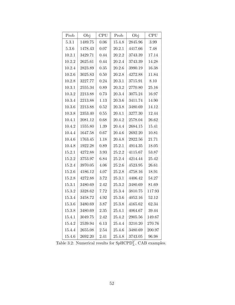
Prob Obj CPU Prob Obj CPU
5.3.1 1489.75 0.06 15.4.8 2845.96 3.99
5.3.6 1478.43 0.07 20.2.1 4417.66 7.48
10.2.1 3429.71 0.44 20.2.2 3743.39 17.14
10.2.2 2625.61 0.44 20.2.4 3743.39 14.28
10.2.4 2823.89 0.35 20.2.6 3990.19 16.38
10.2.6 3025.83 0.50 20.2.8 4272.88 11.84
10.2.8 3227.77 0.24 20.3.1 3715.91 8.10
10.3.1 2555.34 0.89 20.3.2 2770.80 25.16
10.3.2 2213.88 0.73 20.3.4 3075.24 16.97
10.3.4 2213.88 1.13 20.3.6 3411.74 14.90
10.3.6 2213.88 0.52 20.3.8 3480.69 14.12
10.3.8 2353.40 0.55 20.4.1 3277.30 12.44
10.4.1 2081.12 0.68 20.4.2 2578.04 26.62
10.4.2 1555.80 1.39 20.4.4 2684.15 15.41
10.4.4 1647.58 0.67 20.4.6 2692.20 10.81
10.4.6 1763.45 1.18 20.4.8 2922.56 21.71
10.4.8 1922.28 0.89 25.2.1 4914.35 18.05
15.2.1 4272.88 3.93 25.2.2 4115.67 53.87
15.2.2 3753.97 6.84 25.2.4 4214.44 25.42
15.2.4 3970.05 4.06 25.2.6 4523.95 26.61
15.2.6 4186.12 4.07 25.2.8 4758.16 18.91
15.2.8 4272.88 3.72 25.3.1 4406.42 54.27
15.3.1 3480.69 2.42 25.3.2 3480.69 81.69
15.3.2 3328.62 7.72 25.3.4 3810.75 117.93
15.3.4 3458.72 4.92 25.3.6 4052.16 52.12
15.3.6 3480.69 3.87 25.3.8 4165.62 62.34
15.3.8 3480.69 2.35 25.4.1 4064.67 39.44
15.4.1 3049.75 2.42 25.4.2 2905.56 149.67
15.4.2 2539.94 6.13 25.4.4 3210.20 270.76
15.4.4 2655.08 2.54 25.4.6 3480.69 200.97
15.4.6 2692.20 2.41 25.4.8 3743.05 96.98
Table 3.2: Numerical results for SpHCPDVL , CAB examples.
52

Prob Obj CPU Prob Obj CPU
5.2 49424 0.05 25.4 72022 53.63
5.3 30973 0.06 25.5 66953 29.83
10.2 79857 1.06 25.10 45553 5.63
10.3 59522 0.85 40.2 118406 270.62
10.4 55998 0.59 40.3 103972 828.23
10.5 45453 0.57 40.4 88333 1025.70
20.2 90874 9.00 40.5 81401 820.31
20.3 77681 29.39 40.10 52807 259.80
20.4 68648 21.20 50.2 118194 882.46
20.5 60880 12.77 50.3 102390 1077.73
20.10 40860 3.79 50.4 93490 1093.30
25.2 99611 52.51 50.5 77119 1080.28
25.3 84007 43.91 50.10 58359 1008.95
Table 3.3: Numerical results for SpHCPDVL , AP examples.
Step size test for SpHCPDVL
In this section we conduct a study on how the size of the step functions in SpHCPDVL
affects the solution outputs. We randomly chose five test problems of varying size from
the CAB library to conduct the test on. We solved each test problem using a step size
of L = {9, 49, 199, 499}. In four out of the five cases, each solution using the different
step sizes resulted in identical location-allocation solutions. The objective values do
decrease slightly with an increasing step size, due to better found departure times, and
are reported below.
The fifth problem, test problem 10.3.4, gave the same location-allocation solution for
L = 9, L = 49 and L = 499 but not for L = 199. However, it did give the same optimal
objective value as L = 499 which itself only differed 0.01 from the other two step size
solutions which were equivalent. This simply suggests that non-unique optimal location-
allocation solutions exist for 10.3.4. The test results are in other words very promising
and seem to suggest that SpHCPDVL may very well be finding the optimal location-
allocation solution to SpHCPDV with a step size of only L = 9, from proposition 3.2.1,
for these test problems.
53
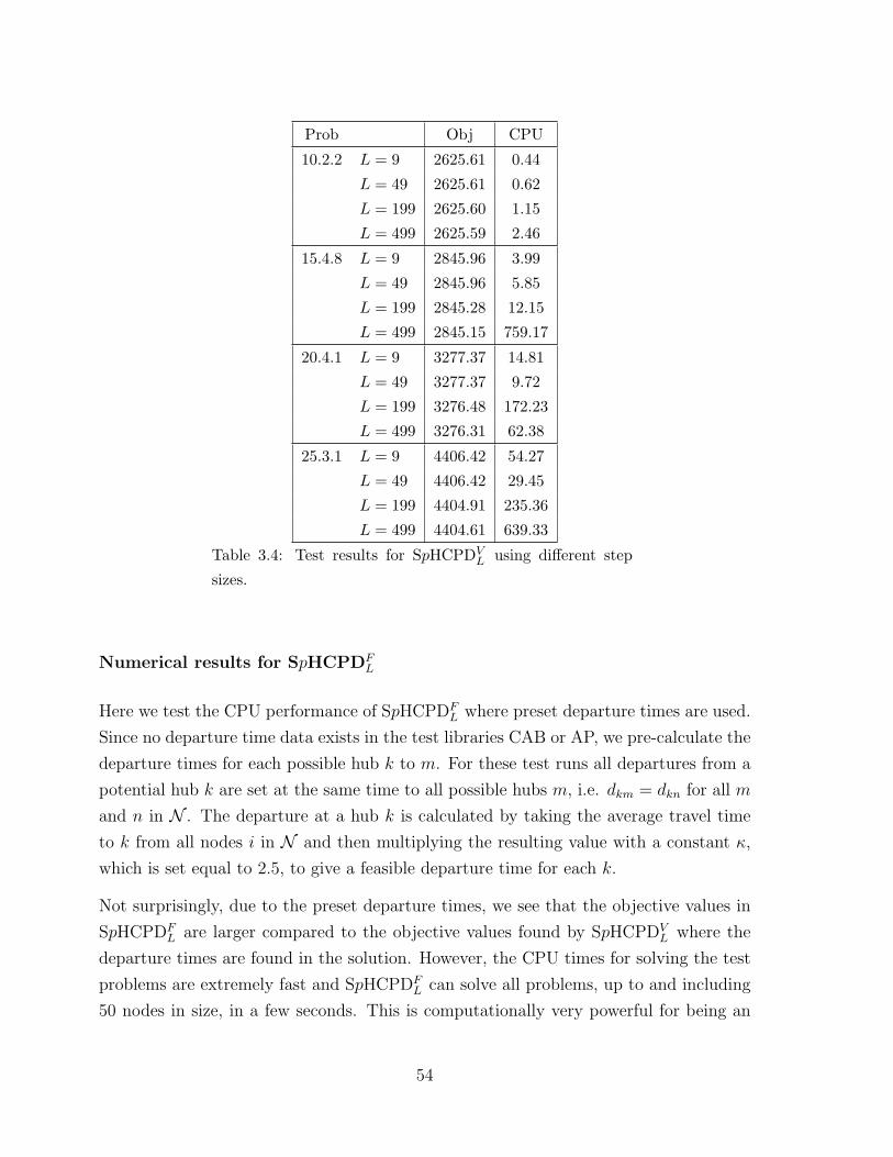
Prob Obj CPU
10.2.2 L = 9 2625.61 0.44
L = 49 2625.61 0.62
L = 199 2625.60 1.15
L = 499 2625.59 2.46
15.4.8 L = 9 2845.96 3.99
L = 49 2845.96 5.85
L = 199 2845.28 12.15
L = 499 2845.15 759.17
20.4.1 L = 9 3277.37 14.81
L = 49 3277.37 9.72
L = 199 3276.48 172.23
L = 499 3276.31 62.38
25.3.1 L = 9 4406.42 54.27
L = 49 4406.42 29.45
L = 199 4404.91 235.36
L = 499 4404.61 639.33
Table 3.4: Test results for SpHCPDVL using different step
sizes.
Numerical results for SpHCPDFL
Here we test the CPU performance of SpHCPDFL where preset departure times are used.
Since no departure time data exists in the test libraries CAB or AP, we pre-calculate the
departure times for each possible hub k to m. For these test runs all departures from a
potential hub k are set at the same time to all possible hubs m, i.e. dkm = dkn for all m
and n in N . The departure at a hub k is calculated by taking the average travel time
to k from all nodes i in N and then multiplying the resulting value with a constant κ,
which is set equal to 2.5, to give a feasible departure time for each k.
Not surprisingly, due to the preset departure times, we see that the objective values in
SpHCPDFL are larger compared to the objective values found by SpHCPDV
L where the
departure times are found in the solution. However, the CPU times for solving the test
problems are extremely fast and SpHCPDFL can solve all problems, up to and including
50 nodes in size, in a few seconds. This is computationally very powerful for being an
54

exact solution formulation to a stochastic p-hub location problem.
Prob Obj CPU Prob Obj CPU
5.3.1 2739.09 0.04 15.4.8 4733.14 0.30
5.3.6 2493.88 0.05 20.2.1 5821.31 0.61
10.2.1 4220.99 0.10 20.2.2 4853.97 0.53
10.2.2 3420.11 0.12 20.2.4 5096.31 0.63
10.2.4 3615.17 0.11 20.2.6 5337.98 0.52
10.2.6 3817.11 0.11 20.2.8 5579.64 0.55
10.2.8 4019.05 0.15 20.3.1 5078.66 0.65
10.3.1 4220.99 0.13 20.3.2 4324.26 0.47
10.3.2 3406.88 0.10 20.3.4 4384.23 1.05
10.3.4 3535.26 0.11 20.3.6 4595.33 1.01
10.3.6 3774.55 0.13 20.3.8 4837.00 0.76
10.3.8 4013.85 0.13 20.4.1 5078.66 0.75
10.4.1 4220.99 0.14 20.4.2 4324.26 0.36
10.4.2 3406.88 0.12 20.4.4 4353.66 0.85
10.4.4 3535.26 0.11 20.4.6 4595.32 0.80
10.4.6 3774.55 0.11 20.4.8 4837.00 0.64
10.4.8 4013.85 0.12 25.2.1 5718.37 1.25
15.2.1 5729.99 0.24 25.2.2 4792.52 1.42
15.2.2 4731.39 0.15 25.2.4 5045.48 1.44
15.2.4 5005.00 0.20 25.2.6 5286.22 1.73
15.2.6 5246.66 0.19 25.2.8 5502.29 1.33
15.2.8 5488.33 0.21 25.3.1 5207.32 0.92
15.3.1 4974.84 0.23 25.3.2 4677.12 1.12
15.3.2 4221.27 0.17 25.3.4 4677.12 0.52
15.3.4 4280.42 0.26 25.3.6 4723.99 0.57
15.3.6 4491.51 0.21 25.3.8 4965.65 1.77
15.3.8 4733.17 0.24 25.4.1 5207.32 0.51
15.4.1 4974.81 0.26 25.4.2 4677.12 0.80
15.4.2 4220.42 0.17 25.4.4 4677.12 1.07
15.4.4 4249.81 0.22 25.4.6 4723.99 1.35
15.4.6 4491.48 0.23 25.4.8 4965.65 1.96
Table 3.5: Numerical results for SpHCPDFL , CAB examples.
55

Prob Obj CPU Prob Obj CPU
5.2 62722 0.03 25.4 103304 1.86
5.3 71154 0.04 25.5 103304 1.51
10.2 81661 0.18 25.10 103304 4.24
10.3 79742 0.13 40.2 135659 6.45
10.4 80716 0.10 40.3 112144 9.73
10.5 81975 0.15 40.4 112144 10.39
20.2 102596 0.79 40.5 112144 31.35
20.3 92824 0.97 40.10 112144 10.50
20.4 91779 0.87 50.2 127218 13.06
20.5 91779 1.84 50.3 115588 34.08
20.10 92820 0.84 50.4 112324 37.71
25.2 109210 1.98 50.5 112324 41.65
25.3 103304 1.90 50.10 112324 30.28
Table 3.6: Numerical results for SpHCPDFL AP, examples.
3.3 The Service Cost Problem
The deterministic and stochastic p-hub center problems, as discussed above, aim to min-
imize the longest path in the network. This is important to consider since an important
aspect for any transportation company to have, to be competitively strong, is to be able
to provide fast delivery times for all origin-destination paths. The stochastic version
of the problem further looks at the reliability of the paths and finds a network setup
such that the maximum delivery time is not breached for at least a probability γ. For
some delivery networks however, there may already exist a natural maximum delivery
time, such as a 24 hour delivery service, which the transportation company wishes to
meet. In these cases the delivery service aspect of the design process comes down to
the reliability of delivering under such a time. In our talks with the different delivery
companies it became clear that apart from a path based reliability it is also important
to consider volume based reliability, i.e. to look at the total percent of packages that
make it on time instead of considering the percent of times a path makes it on time.
The main problem which all transportation companies face is minimizing the overall cost.
When an OD pair misses its delivery time guarantee a cost is incurred on the company.
56

This cost may for example be in overtime working hours, refunds to customers due to
service failure or loss of unhappy customers to the competition in the future. This goes
hand in hand with the volume associated with the OD pair in question and, hence, the
importance of considering the total percent of packages that miss or make their delivery
time guarantees.
To tackle this problem we introduce a new model, which we call the Service Cost Problem
(SCP), which aims to minimize the costs involved, given a maximum delivery time, if
an OD pair does not meet its delivery guarantee. We base this model in accordance
with companies that do not have their own aircraft for the hub-hub links and therefore
look to rent cargo space for the hub link transfers as discussed in Section 3.2.2. Due
to computational complexities, we make a simplification to the network setup but one
which has minimal impact on the solution quality. Instead of considering a location
problem (finding hub locations and node-hub allocations) we instead consider only the
allocation part of the problem for a given hub set. We find that for companies which
rent cargo space this simplification does not affect the network setup by much, since
such companies already know where there is space to be rented and which of these hubs
they wish to utilise for their network design, hence a fixed hub set is already more or
less given.
3.3.1 Stochastic formulation
Working off the same notations as in Section 3.2, we define Cij to be the cost function
representing the cost if an OD pair misses its service guarantee. Each of the costs are
associated with the expected volume on the respective OD pairs. The objective is to
minimize the sum product of Cij multiplied with the probability for the OD path not
meeting the given delivery time β̃ which, for example, may be the latest arrival time
needed to make the departure of the local delivery truck delivering all packages and
letters to the local buildings in the area. Given the set of departure times dkm for all
hub nodes in the hub set H of size p, we can calculate, prior to solving the model, the
departure times Am from hub m to node j, which we here call dm. We do this by setting
dm = maxk
(dkm + αtkm), ∀m ∈ H.
57

This lets us formulate the following single allocation stochastic program.
(SCP)
min.Xik
∑i,j∈N
Cij∑k,m∈H
Pr[T 1ik > dkm ∪ dm + T 2
mj > β̃]XikXjm (3.36)
s.t.∑k∈H
Xik = 1, ∀i ∈ N \ H (3.37)
Xkk = 1, ∀k ∈ H (3.38)
Xik ∈ {0, 1}, ∀i ∈ N ,∀k ∈ H. (3.39)
The objective function (3.36) minimizes the sum of the cost for possibly missing the
delivery time for each OD pair. Pr[T 1ik > dkm ∪ dm + T 2
mj > β̃] is the probability that
packages on path i − k − m − j are not delivered under the given maximum delivery
time β̃, i.e. either link i − k will not make the departure at hub k or the departure
from hub m or the travel time from m to j will get delayed missing the delivery time
β̃. Constraint (3.37) makes sure each node is connected to exactly one hub where (3.38)
assigns each hub to be allocated to itself. (3.39) is the binary constraint.
3.3.2 Reformulations
Due to the difficulty of solving the objective function (3.36) we formulate two linear
equivalent reformulations to SCP in addition to an exact separation algorithm in pursuit
of finding a computationally effective solution approach.
We start by making the objective function linear by adding N2 variables and N2p con-
straints resulting in formulation SCP1 presented below. Next we develop a second for-
mulation, SCP2, to see if one computationally outperforms the other. Due to the fact
that p is often small in comparison to N , we develop this formulation using O(N2p2)
variables but with a factor p fewer constraints than SCP1. Although SCP1 only has
N2p+N constraints, a separation algorithm is developed based on SCP1 which initially
removes N2p constraints to see if this can be computationally beneficial. A separation
algorithm is not developed for SCP2 since the number of constraints here is even smaller.
Due to the fact that the hub set and departure times are known we can first calculate
the probability for each of the possible paths for each OD pair missing the delivery
guarantee, i.e. the probability Pr[T 1ik > dkm ∪ dm + T 2
mj > β̃] for all i, j in N and k,m
in H. Since T 1ik and T 2
mj are independent normal distributions we can easily calculate
58

γijkm where
γijkm = Pr[T 1ik > dkm ∪ dm + T 2
mj > β̃]
= 1− Pr[T 1ik ≤ dkm ∩ dm + T 2
mj ≤ β̃]
= 1− Pr[T 1ik ≤ dkm]Pr[dm + T 2
mj ≤ β̃].
If however T 1ik and T 2
mj are non-normal distributions γijkm could instead be estimated
via simulation and/or sampling. By replacing Pr[T 1ik > dkm ∪ dm + T 2
mj > β̃] in (3.36)
with γijkm we get the equivalent quadratic reformulation of SCP.
(SCPQ)
min.Xik
∑i,j∈N
Cij∑k,m∈H
γijkmXikXjm (3.40)
s.t. (3.37), (3.38), (3.39)
We make the quadratic term in (3.40) linear by introducing a set of continuous decision
variables Vij. Vij is set equal to∑
k,m∈H γijkmXikXjm which is equivalent to Vij ≥∑k∈H γijkm(Xik + Xjm − 1) for all m in H since each node is connected to exactly one
hub. This results in formulation SCP1.
(SCP1)
min.Xik,Vij
∑i,j∈N
CijVij (3.41)
s.t. Vij ≥∑k∈H
γijkm(Xik +Xjm − 1), ∀i, j ∈ N ,∀m ∈ H (3.42)
Vij ≥ 0, ∀i, j ∈ N (3.43)
(3.37), (3.38), (3.39)
Next we formulate SCP2 which has more variables but fewer constraints than SCP1.
Instead of the continuous decision variables Vij we introduce the positive continuous
decision variables Zijkm which are equal to one if OD pair i− j goes via hubs k and m
59

respectively.
(SCP2)
min.Xik,Zijkm
∑i,j∈N
Cij∑k,m∈H
γijkmZijkm (3.44)
s.t.∑k,m∈H
Zijkm = 1, ∀i, j ∈ N , (3.45)
MXik ≥∑j∈N
∑m∈H
Zijkm, ∀i ∈ N ,∀k ∈ H (3.46)
MXjm ≥∑i∈N
∑k∈H
Zijkm, ∀j ∈ N ,∀m ∈ H (3.47)
Zijkm ≥ 0, ∀i, j ∈ N ,∀k,m ∈ H (3.48)
(3.37), (3.38), (3.39)
The objective function (3.44) is equivalent to (3.40), which in turn is equivalent to (3.36),
since constraint (3.45) allows there to be only one path for each OD pair. Additionally,
constraints (3.46) and (3.47) allow only a path to be valid if i is connected to k and j
to m, respectively. M is a big constant.
The separation algorithm we construct for SCP1 is similar to that in [33]. The algorithm
iterates around a master problem and a subproblem which respectively solves a cut down
version of SCP1 and then checks if an optimal solution has been found for SCP1. The
steps of the algorithm are outlined below, and a more detailed description can be found
in [33].
(SCP1-Push)
Step 1 Generate an initial master problem by removing all of the constraints of type
(3.42) in SCP1.
Step 2 Solve the most recently generated master problem. Let X∗ik and V ∗ij be its
optimal solutions.
Step 3 Solve the subproblem by checking constraint violations for (3.42) when X∗jm = 1.
If there is no constraint violation an optimal solution has been found. Otherwise
go to Step 4.
Step 4 Generate a new master problem by adding the new constraint violations from
Step 3 to the master problem. Go to Step 2.
60

3.3.3 Numerical results
In this section we test the computational performance of SCP1, SCP2 and SCP1-Push.
Numerical tests are conducted using an identical setup as described in Section 3.2.3.
Departure times from each hub k to hub m are calculated in the same way as described
in Section 3.2.3. The fixed hub set for each test problem consists of the hub nodes
found from solving SpHCPDFL , presented in Section 3.2.2, for each of the respective test
problems in the CAB and AP libraries. Cij is calculated by taking the average volume
between each OD pair given by the test libraries multiplied with 1000.
In the tables below for each test problem (Prob) we present the optimal objective func-
tion (Obj) and CPU times in seconds for each of the three solution approaches SCP1,
SCP2 and SCP1-Push respectively as well as the number of iterations (Iter) required to
find the optimal solution using SCP1-Push.
CPU performance on the CAB test problems is relatively similar for all three solution
approaches as can be seen in table 3.7. For the AP test problems, table 3.8, we can
see that for some of the test problems, specifically 25.10 and 40.10, SCP1 and SCP1-
Push, respectively, take relatively long to solve. It is well known that different ILP
formulations for the same problem can result in large variations in CPU times due to
the fact that different formulations may require more or less of the branch & bound
tree to be searched before an optimal solution is found, as often demonstrated with the
famous pigeon hole problem [34]. It is observed from the computational runs here that
solving SCP1, and the subproblems in SCP1-Push, for 25.10 and 40.10 respectively, the
branch & bound method struggles to make progress, closing the gap between the lower
and upper bounds, requiring a larger portion of the tree to be searched. For example,
for problem 25.10, solving SCP1, over 500,000 nodes in the tree are searched before
an optimal solution is found. This is compared to solving SCP2 where the initial LP
relaxation of SCP2 finds an optimal integer solution straight away. This naturally has
a major effect on the total CPU time required to solve the problem as can be seen in
table 3.8. An additional observation is that some of the subproblems in SCP1-Push, for
test problem 40.10, are requiring much more of the tree to be searched than if solving
the full formulation, SCP1, directly. This is not uncommon as branch & bound solution
times can sometimes vary drastically, even with only minor changes to the formulation
setup. Thus the results show that using a similar “push” approach as in [33] does, for
the most part, not improve on the computational performance compared to SCP1, and
although all methods give impressive computational results, the winner here is SCP2.
61

Prob Obj SCP1 SCP2 SCP1-Push Iter
5.3.1 214.82 0.02 0.02 0.03 3
5.3.6 335.52 0.01 0.02 0.03 3
10.2.1 125.69 0.03 0.03 0.04 3
10.2.2 647.80 0.04 0.02 0.04 3
10.2.4 333.78 0.02 0.03 0.04 3
10.2.6 187.93 0.02 0.02 0.05 3
10.2.8 149.84 0.02 0.02 0.04 3
10.3.1 122.53 0.03 0.04 0.07 4
10.3.2 256.69 0.03 0.04 0.04 3
10.3.4 228.86 0.03 0.04 0.04 3
10.3.6 183.66 0.03 0.04 0.04 3
10.3.8 146.71 0.03 0.04 0.04 3
10.4.1 122.53 0.04 0.04 0.09 5
10.4.2 256.69 0.04 0.04 0.04 3
10.4.4 228.86 0.04 0.04 0.05 3
10.4.6 183.66 0.04 0.04 0.04 3
10.4.8 146.71 0.04 0.04 0.04 3
15.2.1 1505.59 0.05 0.08 0.07 3
15.2.2 573.61 0.04 0.06 0.06 3
15.2.4 1552.28 0.04 0.04 0.06 3
15.2.6 1534.06 0.05 0.04 0.06 3
15.2.8 1518.72 0.04 0.04 0.06 3
15.3.1 86.35 0.06 0.08 0.08 3
15.3.2 601.26 0.06 0.06 0.10 4
15.3.4 592.92 0.06 0.06 0.08 4
15.3.6 170.51 0.06 0.09 0.09 3
15.3.8 110.97 0.06 0.06 0.06 3
15.4.1 95.09 0.06 0.08 0.10 4
15.4.2 505.47 0.07 0.08 0.11 4
15.4.4 489.93 0.07 0.08 0.09 4
15.4.6 294.21 0.07 0.08 0.10 4
15.4.8 165.61 0.06 0.08 0.10 4
20.2.1 1643.08 0.15 0.21 0.16 3
20.2.2 807.88 0.08 0.09 0.09 3
20.2.4 1695.25 0.09 0.10 0.12 3
20.2.6 1674.93 0.08 0.07 0.10 3
62
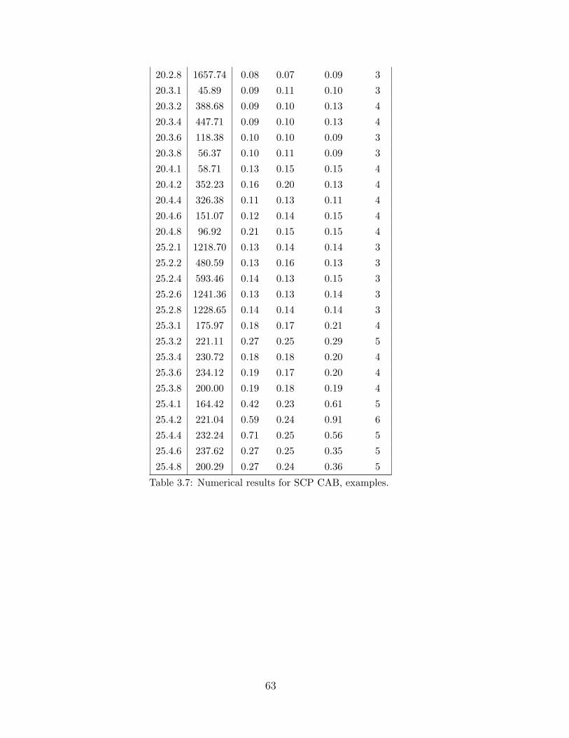
20.2.8 1657.74 0.08 0.07 0.09 3
20.3.1 45.89 0.09 0.11 0.10 3
20.3.2 388.68 0.09 0.10 0.13 4
20.3.4 447.71 0.09 0.10 0.13 4
20.3.6 118.38 0.10 0.10 0.09 3
20.3.8 56.37 0.10 0.11 0.09 3
20.4.1 58.71 0.13 0.15 0.15 4
20.4.2 352.23 0.16 0.20 0.13 4
20.4.4 326.38 0.11 0.13 0.11 4
20.4.6 151.07 0.12 0.14 0.15 4
20.4.8 96.92 0.21 0.15 0.15 4
25.2.1 1218.70 0.13 0.14 0.14 3
25.2.2 480.59 0.13 0.16 0.13 3
25.2.4 593.46 0.14 0.13 0.15 3
25.2.6 1241.36 0.13 0.13 0.14 3
25.2.8 1228.65 0.14 0.14 0.14 3
25.3.1 175.97 0.18 0.17 0.21 4
25.3.2 221.11 0.27 0.25 0.29 5
25.3.4 230.72 0.18 0.18 0.20 4
25.3.6 234.12 0.19 0.17 0.20 4
25.3.8 200.00 0.19 0.18 0.19 4
25.4.1 164.42 0.42 0.23 0.61 5
25.4.2 221.04 0.59 0.24 0.91 6
25.4.4 232.24 0.71 0.25 0.56 5
25.4.6 237.62 0.27 0.25 0.35 5
25.4.8 200.29 0.27 0.24 0.36 5
Table 3.7: Numerical results for SCP CAB, examples.
63
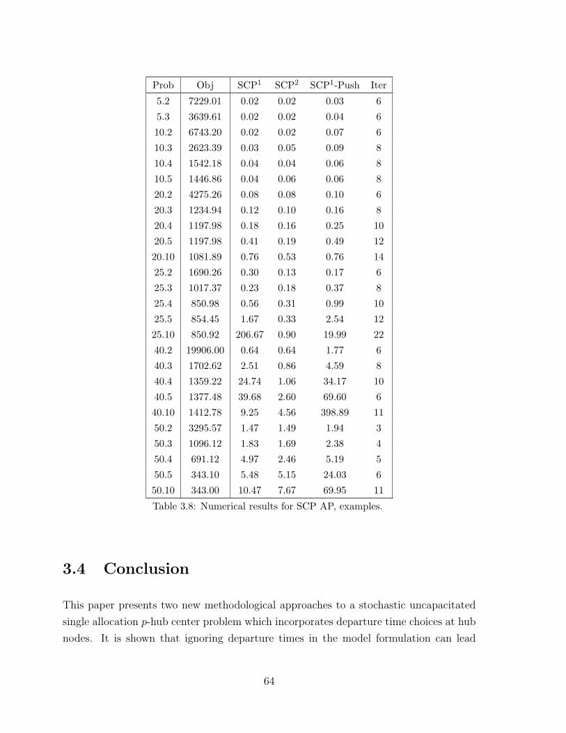
Prob Obj SCP1 SCP2 SCP1-Push Iter
5.2 7229.01 0.02 0.02 0.03 6
5.3 3639.61 0.02 0.02 0.04 6
10.2 6743.20 0.02 0.02 0.07 6
10.3 2623.39 0.03 0.05 0.09 8
10.4 1542.18 0.04 0.04 0.06 8
10.5 1446.86 0.04 0.06 0.06 8
20.2 4275.26 0.08 0.08 0.10 6
20.3 1234.94 0.12 0.10 0.16 8
20.4 1197.98 0.18 0.16 0.25 10
20.5 1197.98 0.41 0.19 0.49 12
20.10 1081.89 0.76 0.53 0.76 14
25.2 1690.26 0.30 0.13 0.17 6
25.3 1017.37 0.23 0.18 0.37 8
25.4 850.98 0.56 0.31 0.99 10
25.5 854.45 1.67 0.33 2.54 12
25.10 850.92 206.67 0.90 19.99 22
40.2 19906.00 0.64 0.64 1.77 6
40.3 1702.62 2.51 0.86 4.59 8
40.4 1359.22 24.74 1.06 34.17 10
40.5 1377.48 39.68 2.60 69.60 6
40.10 1412.78 9.25 4.56 398.89 11
50.2 3295.57 1.47 1.49 1.94 3
50.3 1096.12 1.83 1.69 2.38 4
50.4 691.12 4.97 2.46 5.19 5
50.5 343.10 5.48 5.15 24.03 6
50.10 343.00 10.47 7.67 69.95 11
Table 3.8: Numerical results for SCP AP, examples.
3.4 Conclusion
This paper presents two new methodological approaches to a stochastic uncapacitated
single allocation p-hub center problem which incorporates departure time choices at hub
nodes. It is shown that ignoring departure times in the model formulation can lead
64

to non-optimal design solutions. Both variable and fixed departure time choices are
modeled together with effective solution reformulations. Numerical tests are conducted
showing the efficiency of the solution formulations on network sizes of up to 50 nodes
using the standard CAB and AP test libraries.
In addition a new service cost problem is introduced for an allocation network. A
stochastic formulation is given, where travel time on links are random, and three different
solution approaches are presented. This problem minimizes the cost of origin-destination
pairs missing their service guarantees for a given maximum delivery time. Numerical
results are shown also using the standard CAB and AP test libraries.
65
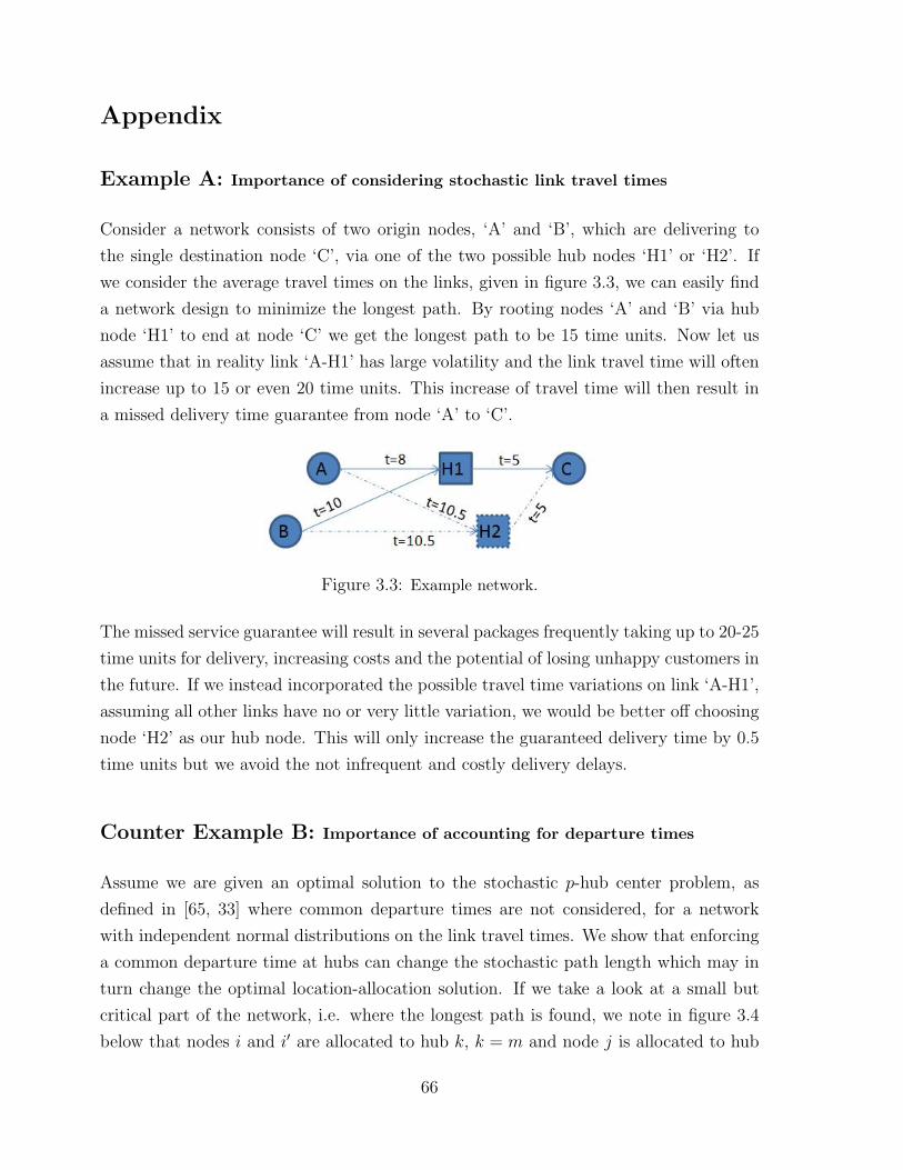
Appendix
Example A: Importance of considering stochastic link travel times
Consider a network consists of two origin nodes, ‘A’ and ‘B’, which are delivering to
the single destination node ‘C’, via one of the two possible hub nodes ‘H1’ or ‘H2’. If
we consider the average travel times on the links, given in figure 3.3, we can easily find
a network design to minimize the longest path. By rooting nodes ‘A’ and ‘B’ via hub
node ‘H1’ to end at node ‘C’ we get the longest path to be 15 time units. Now let us
assume that in reality link ‘A-H1’ has large volatility and the link travel time will often
increase up to 15 or even 20 time units. This increase of travel time will then result in
a missed delivery time guarantee from node ‘A’ to ‘C’.
Figure 3.3: Example network.
The missed service guarantee will result in several packages frequently taking up to 20-25
time units for delivery, increasing costs and the potential of losing unhappy customers in
the future. If we instead incorporated the possible travel time variations on link ‘A-H1’,
assuming all other links have no or very little variation, we would be better off choosing
node ‘H2’ as our hub node. This will only increase the guaranteed delivery time by 0.5
time units but we avoid the not infrequent and costly delivery delays.
Counter Example B: Importance of accounting for departure times
Assume we are given an optimal solution to the stochastic p-hub center problem, as
defined in [65, 33] where common departure times are not considered, for a network
with independent normal distributions on the link travel times. We show that enforcing
a common departure time at hubs can change the stochastic path length which may in
turn change the optimal location-allocation solution. If we take a look at a small but
critical part of the network, i.e. where the longest path is found, we note in figure 3.4
below that nodes i and i′ are allocated to hub k, k = m and node j is allocated to hub
66
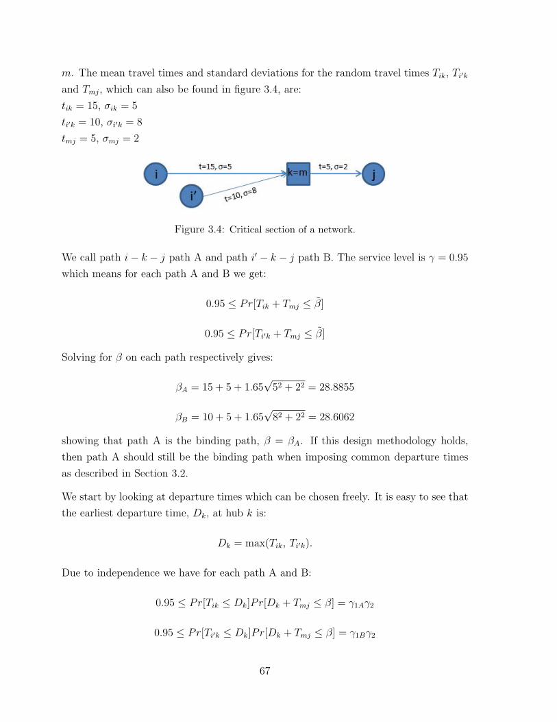
m. The mean travel times and standard deviations for the random travel times Tik, Ti′k
and Tmj, which can also be found in figure 3.4, are:
tik = 15, σik = 5
ti′k = 10, σi′k = 8
tmj = 5, σmj = 2
Figure 3.4: Critical section of a network.
We call path i− k − j path A and path i′ − k − j path B. The service level is γ = 0.95
which means for each path A and B we get:
0.95 ≤ Pr[Tik + Tmj ≤ β̃]
0.95 ≤ Pr[Ti′k + Tmj ≤ β̃]
Solving for β on each path respectively gives:
βA = 15 + 5 + 1.65√
52 + 22 = 28.8855
βB = 10 + 5 + 1.65√
82 + 22 = 28.6062
showing that path A is the binding path, β = βA. If this design methodology holds,
then path A should still be the binding path when imposing common departure times
as described in Section 3.2.
We start by looking at departure times which can be chosen freely. It is easy to see that
the earliest departure time, Dk, at hub k is:
Dk = max(Tik, Ti′k).
Due to independence we have for each path A and B:
0.95 ≤ Pr[Tik ≤ Dk]Pr[Dk + Tmj ≤ β] = γ1Aγ2
0.95 ≤ Pr[Ti′k ≤ Dk]Pr[Dk + Tmj ≤ β] = γ1Bγ2
67
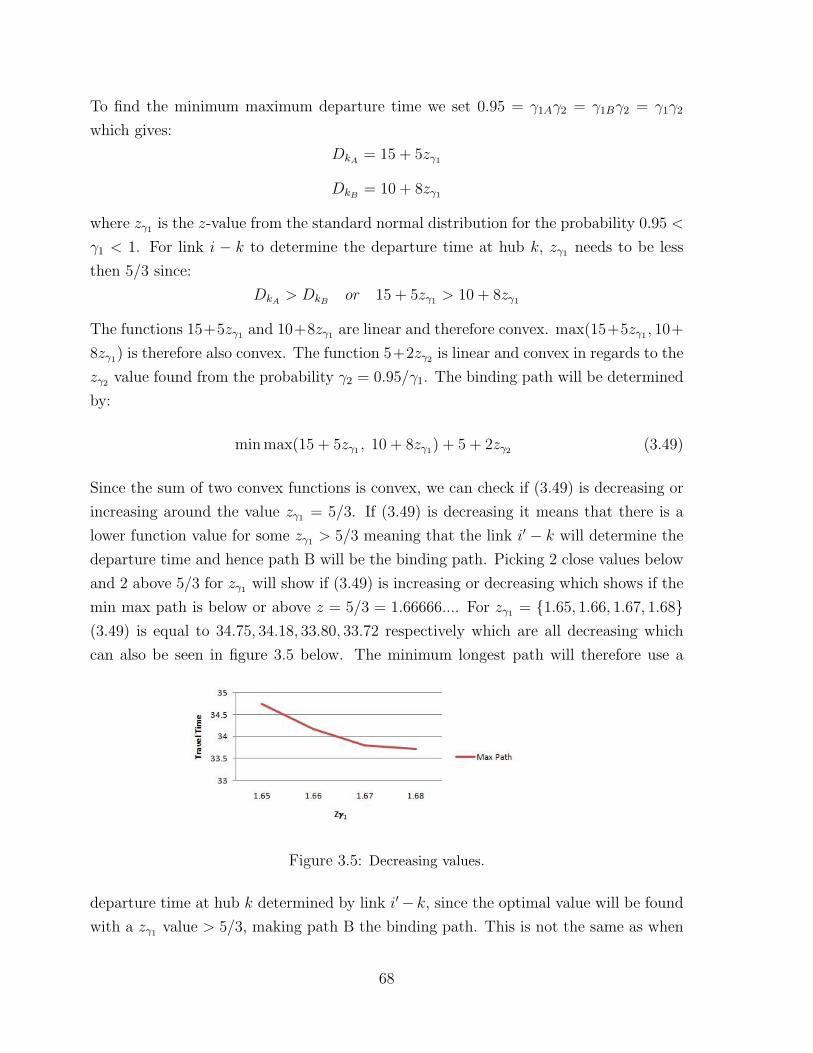
To find the minimum maximum departure time we set 0.95 = γ1Aγ2 = γ1Bγ2 = γ1γ2
which gives:
DkA = 15 + 5zγ1
DkB = 10 + 8zγ1
where zγ1 is the z-value from the standard normal distribution for the probability 0.95 <
γ1 < 1. For link i − k to determine the departure time at hub k, zγ1 needs to be less
then 5/3 since:
DkA > DkB or 15 + 5zγ1 > 10 + 8zγ1
The functions 15+5zγ1 and 10+8zγ1 are linear and therefore convex. max(15+5zγ1 , 10+
8zγ1) is therefore also convex. The function 5+2zγ2 is linear and convex in regards to the
zγ2 value found from the probability γ2 = 0.95/γ1. The binding path will be determined
by:
min max(15 + 5zγ1 , 10 + 8zγ1) + 5 + 2zγ2 (3.49)
Since the sum of two convex functions is convex, we can check if (3.49) is decreasing or
increasing around the value zγ1 = 5/3. If (3.49) is decreasing it means that there is a
lower function value for some zγ1 > 5/3 meaning that the link i′ − k will determine the
departure time and hence path B will be the binding path. Picking 2 close values below
and 2 above 5/3 for zγ1 will show if (3.49) is increasing or decreasing which shows if the
min max path is below or above z = 5/3 = 1.66666.... For zγ1 = {1.65, 1.66, 1.67, 1.68}(3.49) is equal to 34.75, 34.18, 33.80, 33.72 respectively which are all decreasing which
can also be seen in figure 3.5 below. The minimum longest path will therefore use a
Figure 3.5: Decreasing values.
departure time at hub k determined by link i′− k, since the optimal value will be found
with a zγ1 value > 5/3, making path B the binding path. This is not the same as when
68

departure times are not accounted for and hence the given solution may not be optimal
when departure times are added.
For fixed and given departure times, here dk, the same can easily be shown. We set
dk = 23.5 which gives for each path A and B:
0.95/(Pr[Tik ≤ dk]) ≤ Pr[dk + Tmj ≤ β]
0.95/(Pr[Ti′k ≤ dk]) ≤ Pr[dk + Tmj ≤ β]
Solving for β on each path respectively with dk = 23.5 gives:
βA = 33.56
βB = 33.7
showing that path B is now the binding path, β = βB, and the solution found with the
original model is non-optimal.
69

Chapter 4
Paper Three
Modeling Risk in the Capacitated Single AllocationHub Location Problem
Edward Hult
Judge Business School, University of Cambridge, Trumpington Street, Cambridge CB2 1AG,
United Kingdom, {[email protected]}
Abstract
The capacitated single allocation hub location problem aims to design a hub and spoke
network minimizing the total flow and hub setup costs. Hub capacity limits are modeled
as constraints based on average flow volumes. This may however result in big capac-
ity breaches at hub nodes and can lead to high costs and poor service quality across
the network. We propose extending the deterministic version by introducing stochastic
origin-destination flow volumes to account for the risk of breaching hub capacity lim-
its. We formulate a chance constraint model incorporating the conditional value-at-risk
which is a safe measure to assure capacity limits are not breached with at least a prob-
ability γ. In addition, we propose a linear sample average approximation model as a
strong solution method, whose solution converges to a solution of the original problem
70
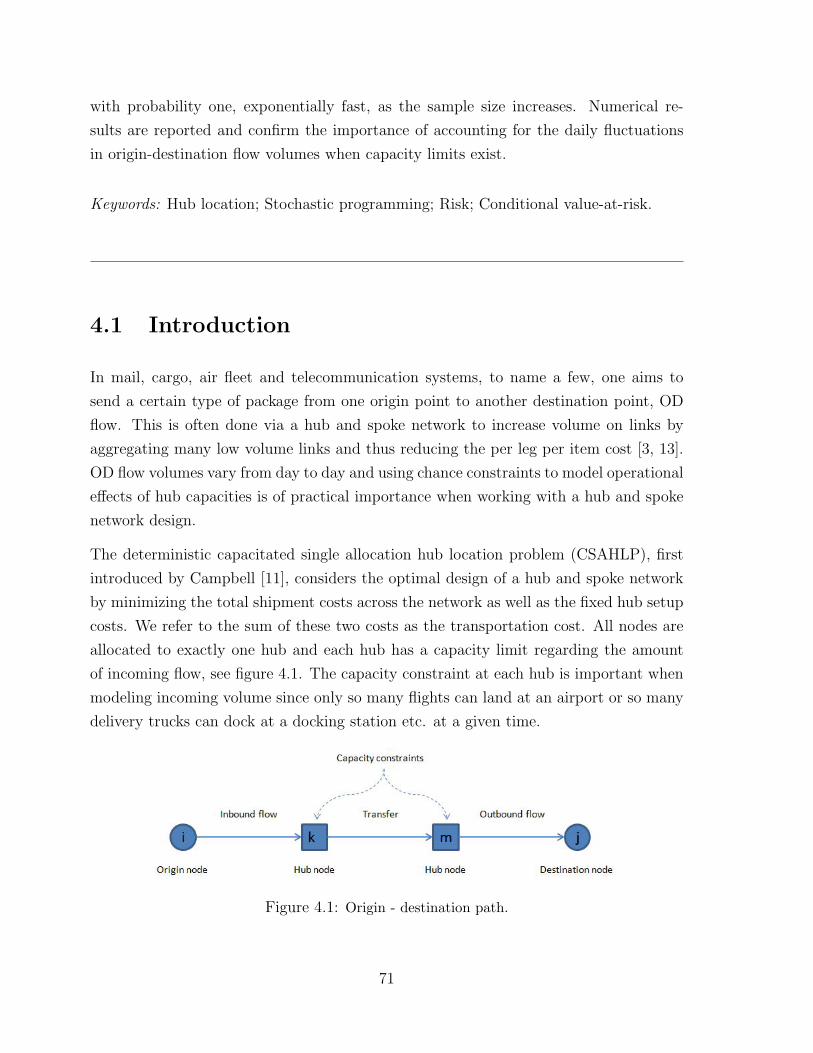
with probability one, exponentially fast, as the sample size increases. Numerical re-
sults are reported and confirm the importance of accounting for the daily fluctuations
in origin-destination flow volumes when capacity limits exist.
Keywords: Hub location; Stochastic programming; Risk; Conditional value-at-risk.
4.1 Introduction
In mail, cargo, air fleet and telecommunication systems, to name a few, one aims to
send a certain type of package from one origin point to another destination point, OD
flow. This is often done via a hub and spoke network to increase volume on links by
aggregating many low volume links and thus reducing the per leg per item cost [3, 13].
OD flow volumes vary from day to day and using chance constraints to model operational
effects of hub capacities is of practical importance when working with a hub and spoke
network design.
The deterministic capacitated single allocation hub location problem (CSAHLP), first
introduced by Campbell [11], considers the optimal design of a hub and spoke network
by minimizing the total shipment costs across the network as well as the fixed hub setup
costs. We refer to the sum of these two costs as the transportation cost. All nodes are
allocated to exactly one hub and each hub has a capacity limit regarding the amount
of incoming flow, see figure 4.1. The capacity constraint at each hub is important when
modeling incoming volume since only so many flights can land at an airport or so many
delivery trucks can dock at a docking station etc. at a given time.
Figure 4.1: Origin - destination path.
71
This paper considers the CSAHLP with stochastic OD flows and accounts for its random
volume fluctuations on a daily basis. When designing networks it is often much easier
to work with, construct and solve deterministic models rather than models accounting
for random or unknown events. However, deterministic models do not always repre-
sent reality closely enough to be beneficial. Here for example, volume is an important
parameter which is far from static but is a key component in the deterministic CSAHLP.
When considering stochastic volume there are two types of situations which can be
studied. The first, which is often found in stochastic facility location median problems,
is the possible permanent volume changes that may take place in some future event.
The second, which is what we consider here, is the fluctuation of volume generated from
each origin node i on a daily basis. When designing a network based on capacitated flow
volumes it is extremely important to consider this daily fluctuation on each origin node.
It is important since if ignored, or assumed constant, hub nodes may often receive more
flow than they are capable of handling leading to major congestion problems, soaring
costs and poor services by the company. For example, if the average inflowing volume
to a hub is equal to the hub’s capacity, it will lead to an overflow of volume at the
hub up to 50 percent of the time. This is especially true if the volume distributions
from the nodes are tail heavy since this can lead to a breach in capacity more often
than 50 percent of the time. Due to this, the optimal solutions found by the existing
deterministic models in the literature may in actuality give a poor network design. In
addition, the few stochastic models in the literature cannot handle different variations
of OD flow volumes on a daily basis and provide limited benefits for transportation
companies who want to guard against high volume fluctuations of incoming flow to a
hub node during a given time [44, 81, 15]. We therefore propose a new model which
incorporates a risk measure to account for different volume fluctuations from different
origin nodes.
For the CSAHLP with stochastic OD flow volumes, we introduce a chance constraint
formulation which accounts for the risk of breaching the capacity limits at each of the
different hubs. We want to set the value-at-risk (VaR) to be less than or equal to each
hub’s capacity, where the probability of flow exceeding the capacity is not more than
γ. However, VaR is hard to solve since even if a normal distribution is assumed on the
OD flows, one ends up with a non-linear binary formulation which is extremely hard
to solve for any but very small sized networks. We therefore apply the risk measure
conditional value-at-risk (CVaR) [57], also known as expected or mean shortfall and tail
value-at-risk [58]. We here denote CVaR, for each hub k, as CV aRkγ, which states that
72

for a lower value φk, such that φk is not exceeded with a probability γ, then CV aRkγ is
the expected value when φk is exceeded. Since CV aRkγ automatically calculates φk, we
get the capacity at each hub to hold at least γ100% of the time when we set CV aRkγ as
a capacity constraint to be less than or equal to each hub’s capacity limit. This holds
since φk will always be less than or equal to CV aRkγ and is a great strength of the risk
measure.
In addition, we formulate a sample average approximation (SAA) method which we
show also solves the CVaR model with probability one for large enough sample sizes. It
is also shown that it converges exponentially fast with an increase of the sample size.
Convergence statements and their proofs are not new within the SAA literature and it
has been shown that, for models with specific properties, the above statement holds true
[5, 39]. We show that the SAA convergence proof presented for the models in Atlason
et al. [5] also holds true for our models. We can therefore find a reliable solution which
solves for a safe VaR while considering the important random OD flow fluctuations.
In Section 4.1.1 we review the hub and spoke literature as well as the facility location lit-
erature in regards to stochastic and deterministic hub location problems and stochastic
demand median problems, respectively. In Section 4.2 we model the stochastic CSAHLP
with chance constraints. In Section 4.3 we formulate the SAA model and show that the
solution found for the SAA model converges to the solution of the original model with
an increasing sample size. In Section 4.4 we give an equivalent but smaller sized linear
formulation which can be solved using any standard mixed integer linear programing
solver. In Section 4.5 several numerical tests are conducted on up to 50 node networks.
Simulation runs are also conducted on the optimal network setups found from our pro-
posed model as well as the optimal solution from the existing deterministic models, which
confirm the importance of modeling stochastic volume when considering hub capacities.
4.1.1 Literature review
The capacitated single allocation hub location problem was first introduced by Campbell
[11] who formulated a linear model with O(n4) variables and constraints. This model
was later computationally improved by Ernst et al. [28] who used the uncapacitated
p-hub median model from Ernst et al. [25] to formulate a tighter CSAHLP model. This
formulation has been the computationally fastest MILP formulation, but was shown
recently by Correia et al. [17] to be incomplete for some problems, giving infeasible values
73
to some variables. To fix this they added an additional set of constraints. A variation
to the standard problem is presented by Costa et al. [18], who remove the capacity
constraint and instead add a second objective function to the formulation minimizing
the time a hub takes to process the incoming flow. This was done to try to spread
out the volume more cost beneficially without using a hard constraint on the maximum
capacity.
For stochastic hub and spoke network design there is a limited pool of existing research.
There are a few papers on stochastic hub location problems but none of these accounts
for different variations of stochastic volume originating from each origin node when ca-
pacity constraints are present. Marianov and Serra [44] build an M/D/c queuing model
for the number of airplanes waiting to land assuming Poisson arrivals of airplanes. They
solve the capacitated multiple allocation hub location problem with capacity constraints
on the number of airplanes allowed in the queue for some probability. The queuing
model calculates the capacity beforehand and then they set the average incoming flights
to each hub to be less than or equal to the found maximum capacity. They develop
a heuristic algorithm based on tabu search and solve up to 30 node networks. Yang
[81] looks at an air freight uncapacitated multiple allocation hub location problem with
stochastic demand and stochastic discount factors on the hub-hub links. They formu-
late a two stage model where the first is a deterministic model, taking into account the
solution found from the second stage model, and solves for the number and locations of
hub nodes. The second stage solves the flight routing problem considering the stochas-
tic properties. This is reformulated into one extended model considering three discrete
scenarios of the stochastic outcomes. They look at and solve a case study of a 10 node
air freight network in Taiwan and China. Contreras et al. [15] look at the stochastic
uncapacitated hub location problem with random demand and random transportation
costs. They show that considering stochastic demand, when no capacity constraints
exist, or stochastic dependent transportation costs results in the same models as the
respective deterministic models. They then move on to model the uncapacitated hub
location problem with stochastic independent transportation costs which they approx-
imately solve, using Monte-Carlo simulation coupled with Benders’ decomposition, for
up to 50 node networks. None of the existing hub location papers, however, consider the
daily fluctuations of the OD flow volumes for networks which have capacity constraints
on the incoming flow to each hub. Since many hub and spoke networks have constraints
on the amount of flow their hub nodes can efficiently handle, this is a significant gap in
the literature. Filling this gap is the main contribution of this paper.
74

In addition to the three hub location problems, Sim et al. [65] consider stochastic
travel times for the single allocation p-hub center problem. They assume independent
normal distributions on the travel times for each link and develop heuristic methods to
approximately solve network sizes up to 40 nodes. Hult et al. [33] look at the same
stochastic p-hub center problem as in [65] but present exact solution methods based on
preprocessing and a separation algorithm to solve up to 50 node networks.
There is a much larger pool of stochastic research done in the facility location literature.
Looking at the literature using uncertain demand for median type problems there is one
big difference however, which is that most facility location problems look at how demand
might permanently change in the future and thus change the cost of flow through the
network, differing from the every day fluctuations we are interested in. Earlier work on
the stochastic demand p-median facility location problem used a mean outcome model
where the expected volume was calculated from different possible scenarios of how future
demand may look, see for example Sheppard [64] and Weaver and Church [78]. Louveaux
[43] presents a similar version of the p-median problem but includes capacity constraints
and instead maximizes the expected utility of profit. Carbone [14] minimizes a chance
constrained upper bound on the total demand weighted distance, choosing p facilities to
hold for a given probability. Zhou and Liu [83] present a few different risk models for
the capacitated median facility location problem. Demand is stochastic and due to the
capacity constraints at the facilities, customers may not only be supplied by the nearest
factory. They set up three different formulations, an expected value model which is
linear, a chance-constrained model which provides a confidence level β (minimizing the
value which the cost needs to be less than for a probability β), and also a dependent-
chance model which maximizes the probability that the cost does not exceed some given
value. They then solve these approximately by using a hybrid intelligent algorithm
consisting of simulations, a genetic algorithm and the simplex algorithm. Wen and
Iwamura [79] solve the same stochastic facility location-allocation problem as [83] above.
They model it as a chance-constrained model as well but under the Hurwicz criterion,
i.e. a weighted balance between minimizing the value which the cost should be less than
for some confidence level and the min-max value which the cost should be more than for
the same confidence level. They then solve this model using fuzzy simulation. Wang [76]
uses probabilistic demand constraints for the median location problem, minimizing the
total travel cost with unknown demand and then solves this exactly by considering all
possible combinations of random demands. This model can however only be used to solve
small networks. He also approximates the problem by assuming normal distributions but
75
exact solution times are still very large for small sized problems. Albareda-Sambola et al.
[2] formulate the facility location problem with Bernoulli demands. They set capacity
constraints for the facilities and use a penalty cost if demand exceeds the capacity.
They also require a minimum number of customers to be allocated to a facility for it
to be opened. They solve the resulting stochastic assignment problem both by using
simulation and a heuristic algorithm. Wagner et al. [75] formulate the uncapacitated
median facility location problem with stochastic demands. They model it using the risk
measure value-at-risk borrowed from the finance literature which minimizes the value
the cost needs to be less than or equal to for a given probability/risk. They solve
this using simulated data and by deriving a convex nonlinear program and design a
branch-and-bound algorithm. Their initial model can solve problems up to 25 nodes
in size, they can however solve problems up to 40 nodes in some special cases. There
are many different variations to the stochastic facility location problem that consider
different objective functions and/or other stochastic properties in comparison to the
median type problems mentioned here. The interested reader is referred to, for more
details on different stochastic facility location problems, the literature review paper by
Snyder [69].
4.2 The Stochastic Capacitated Single Allocation
Hub Location Problem
We here introduce the CSAHLP with stochastic OD flows using chance constraints,
V aRkγ. To make this computationally feasible, we immediately remodel via CV aRk
γ.
This safely sets V aRkγ less than or equal to the capacity limit at each hub for a given
probability. We refer to this model as the stochastic capacitated single allocation hub
location problem with chance constraints or, stochastic capacitated hub location problem
(SCHLP), for short.
Define a set of nodes N to be allocated to an unknown set of hub nodes H ⊆ N .
Each node i is allocated to exactly one hub and all hub nodes are assumed to be fully
connected. The shipment cost per unit flow from node i to k is represented by tik and
Xik is the binary variable which is equal to one if and only if node i is allocated to k
for all i, k ∈ N . Since each node is allocated to itself if it is a hub node Xkk equals one
if node k is a hub. Zijkm are the binary variables which are equal to one if and only
76

if the path OD pair i − j takes is via hub nodes k and m. χ, δ and α are economies
of scale where α, which is less than or equal to both χ and δ, is the economy of scale
for consolidation. Fk is the fixed hub setup cost at node k and Γk is the maximum
capacity at hub k. Let ζ denote the probability distribution of the random flow volume
where Wij(ζ) is the stochastic volume of flow between OD pair i − j. Wij is the mean
and σ̃2ij is the variance of Wij(ζ). We also define Oi(ζ) as the stochastic volume of flow
generated at origin node i where Oi(ζ) =∑
jWij(ζ). Oi is the mean and σ2i is the
variance of Oi(ζ). Similarly we define Dj(ζ) as the stochastic demand of flow arriving
at node j where Dj(ζ) =∑
iWij(ζ) and Dj is the mean and σ̂2j the variance of Dj(ζ).
Additionally Hk( ~O(ζ), ~Xk) is the total volume flowing into hub k which is dependent
on the decision variables Xik, Hk( ~O(ζ), ~Xk) =∑
i∈N Oi(ζ)Xik. V aRkγ(Hk( ~O(ζ), ~Xk)) is
the value-at-risk for SCHLP, which is the value, depending on the chosen hub k, which
the total volume flowing into the hub will not exceed by a probability γ. Similarly the
conditional value-at-risk, CV aRkγ(Hk( ~O(ζ), ~Xk)), is the expected volume of flow into
each hub k conditional on flow exceeding V aRkγ(Hk( ~O(ζ), ~Xk)).
We formulate SCHLP by setting CV aRkγ(Hk( ~O(ζ), ~Xk)) as a constraint. The idea with
the model is to make sure capacity holds at each hub k at least γ100% of the time. Setting
CV aRkγ(Hk( ~O(ζ), ~Xk)) less than or equal to the capacity of hub k ensures that the
associated VaR constraint holds, namely, capacity is not breached more than γ100% of
the time. This is actually very robust with respect to minimizing the chance of breaching
the capacity constraint when high values of γ are used, see Section 4.5.3. In addition to
approximating V aRkγ(Hk( ~O(ζ), ~Xk)), CV aR
kγ(Hk( ~O(ζ), ~Xk)), used as a constraint, has
an added benefit. It guards against extreme volume events the (1− γ)100% of the time
the capacity does not hold, by, for example, denying several origin nodes with tail heavy
flow distributions to be assigned to the same hub. We now formulate SCHLP using the
decision variables Xik and Zijkm.
77

(SCHLP) min.Xik,Zijkm
E[∑i,k∈N
tikXik(χOi(ζ) + δDi(ζ))] + E[∑
i,j,k,m∈N
αtkmWij(ζ)Zijkm] +∑k∈N
FkXkk (4.1)
s.t. 0 ≤ ΓkXkk − CV aRkγ(Hk( ~O(ζ), ~Xk)), ∀k ∈ N (4.2)∑
k∈N
Xik = 1, ∀i ∈ N (4.3)
Xik ≤ Xkk, ∀i, k ∈ N (4.4)∑k,m∈N
Zijkm = 1, ∀i, j ∈ N (4.5)
Zijkm ≤ Xik, ∀i, j, k,m ∈ N (4.6)
Zijkm ≤ Xjm, ∀i, j, k,m ∈ N (4.7)
Zijkm ∈ {0, 1}, ∀i, j, k,m ∈ N (4.8)
Xik ∈ {0, 1}, ∀i, k ∈ N (4.9)
The objective function consists of three terms which all define the transportation cost.
The expected shipment cost on node-hub links and hub-node links are respectively cal-
culated in the first term. The expected shipment cost on the hub-hub links is calculated
in the second term and the fixed hub setup cost is calculated in the third term. Con-
straint (4.2) is the approximate chance constraint and sets CV aRkγ(Hk( ~O(ζ), ~Xk)) to be
less than or equal to the capacity at each hub k. Constraint (4.3) allows each node to
be allocated to exactly one hub node and (4.4) forces each node allocation to be to a
hub node. Constraint (4.5) makes sure only one path is chosen for each OD pair and
constraints (4.6) and (4.7) make sure i is connected to k and j is connected to m for the
chosen OD path. Constraints (4.8) and (4.9) are the binary constraints.
A few remarks on the model are in order. First, as mentioned above, any feasible hub
allocation flows through the network will not violate any hub constraints with at least
a probability γ. This can be seen visually in figure 4.2 where CVaRγ is the average
value of the shaded area. Second, one cannot guarantee that a capacity breach will
never occur since extreme instances do happen, but by increasing γ the chance of a
breach is lessened. This however may in turn increase the transportation cost setup
and γ needs therefore to be chosen in regard to the user’s risk preference. Thirdly,
similar to the deterministic models, it is assumed that at each node the origin and
demand volumes are similar and therefore here it is also assumed that they have the
78

Figure 4.2: Cumulative distribution graph for total volume flowing into a hub, showing theVaRγ , CVaRγ and the hub capacity, Γ.
same probability distributions. Thus if a hub k can handle the inbound flow from all
nodes i which are allocated to it, it can also later handle all the flow arriving to it
from the other hub nodes due to the same total inbound and outbound flow volumes.
However if this is not the case then one can simply modify the above formulation by
adding the additional set of risk constraints 0 ≤ ΓkXkk − CV aRkγ(H
′k(~D(ζ), ~Xk)) for
all k ∈ N , where H ′k(~D(ζ), ~Xk) =
∑i∈N Di(ζ)Xik. This holds since the total transfer
volume arriving to a hub from all other hubs will equal the total outbound volume,∑i∈N Di(ζ)Xik, it delivers.
Since we are not concerned with possible permanent changes to flow volume in the
future but are instead considering daily fluctuations, the total shipment cost function
can be reformulated as a deterministic function using average flow volumes without loss
of precision. This is due to the fact that the location-allocation solution found will,
over time, average out the fluctuating transportation costs associated with the random
volumes. From basic probability theory we know that for some random variables V1 and
V2 and for some constants (or fixed decision variable) a1 and a2, the following expectation
holds:
E[a1V1 + a2V2] = a1E[V1] + a2E[V2]
Therefore we can reformulate the first two terms in the objective function in (4.1) in the
same way.
79

E[∑i,k∈N
tikXik(χOi(ζ) + δDi(ζ))] + E[∑
i,j,k,m∈N
αtkmWij(ζ)Zijkm] +∑k∈N
FkXkk =∑i,k∈N
tikXik(χE[Oi(ζ)] + δE[Di(ζ)]) +∑
i,j,k,m∈N
αtkmE[Wij(ζ)]Zijkm +∑k∈N
FkXkk =∑i,k∈N
tikXik(χOi + δDi) +∑
i,j,k,m∈N
αtkmWijZijkm +∑k∈N
FkXkk (4.10)
This allows us to use the average values for the shipment costs in CSAHLP which can
be formulated as
(SCHLP2) min.Xik,Zijkm
∑i,k∈N
tikXik(χOi + δDi) +∑
i,j,k,m∈N
αtkmWijZijkm +∑k∈N
FkXkk
s.t. 0 ≤ ΓkXkk − CV aRkγ(Hk( ~O(ζ), ~Xk)), ∀k ∈ N
(4.3)− (4.9)
Even though we can use average values for the shipment costs we still have the condi-
tional value-at-risk constraint (4.2) to deal with which is the topic of the next section.
4.3 Sample Average Approximation
Financial models using CVaR can efficiently be estimated for any formulation by using
data sampling to give an LP approximation, see for example [4, 42, 57, 58]. For SCHLP2
the same can be done.
Since the CVaR constraint (4.2) is hard to deal with directly, we can estimate the CVaR
function by taking S data samples from Oi(ζ) for all i ∈ N . This is also referred to as
a sample average approximation (SAA) method. SAA problems are well studied in the
literature where many papers look at convergence rates for different problems, see for
example [5, 39, 77].
Taking S samples of Oi(ζ), denoted as Ois(ζs) for s ∈ S = {1, . . . , S}, we get,
CV aRk
γS(Hk( ~Os(ζs), ~Xk)). CV aRk
γS(Hk( ~Os(ζs), ~Xk)) is a SAA of S independent and
identically distributed realizations of CV aRkγ(Hk( ~O(ζ), ~Xk)) (given explicitly in (4.17)
below), where ζ is replaced by its SAA ζ1, . . . , ζS and CVaR is applied to the corre-
sponding discrete approximation Hk( ~Oi1(ζ1), ~Xik), . . . , Hk( ~OS(ζS), ~Xk) of the original
80
distribution Hk( ~Oi(ζ), ~Xik). This is the average value of these quantities conditional on
not falling below their 100γ percentile. In Section 4.4 we show that for any given Xik
solution
Pr[ limS→∞
CV aRk
γS(Hk( ~Os(ζs), ~Xk)) = CV aRkγ(Hk( ~O(ζ), ~Xk))] = 1, ∀k ∈ N .
Thus we can formulate SCHLP2 as a SAA model, SCHLP2S, as
(SCHLP2S ) min.Xik,Zijkm
∑i,k∈N
tikXik(χOi + δDi) +∑
i,j,k,m∈N
αtkmWijZijkm +∑k∈N
FkXkk
s.t. 0 ≤ ΓkXkk − CV aRk
γS(Hk( ~Os(ζs), ~Xk)), ∀k ∈ N (4.11)
(4.3)− (4.9)
4.3.1 Convergence
Our purpose is to show that the convergence framework of [5] applies above, hence the
following result holds:
Theorem 4.3.1 The optimal solutions of SCHLP2S are a subset of the optimal solutions
of SCHLP2 with probability 1 when S is large. Furthermore a solution of SCHLP2S con-
verges to a solution of SCHLP2 with probability 1 exponentially fast when S is increased,
for example,
Pr[|CV aRk
γS(Hk( ~Os(ζs), ~Xk))− CV aRkγ(Hk( ~O(ζ), ~Xk))| ≥ ε] ≤ ae−bS
for some constants ε, a, b > 0 that are independent of S.
We assume, as in [19] which is used in [5], that ζ ∈ Rm denotes any random variable
that takes values in Rm and for which there exists c > 0, θ0 > 0, η(·) : Rm → R1 such
that
|Hk( ~O(ζ), ~Xk)| ≤ cη(ζ), E[eθη(ζ)] <∞,
for any solution Xik and for all 0 ≤ θ ≤ θ0. This is in accordance with assumptions of
Theorem 3.1 of [19] (to the expectation of (4.17), the SAA of the CV aRkγ(Hk( ~O(ζ), ~Xk)),
given later in Section 4.4).
81
In [5] a generalization of the theorem above is shown to hold in the context of a call
center model where the number of incoming calls are stochastic. Note that [5] insist on
integer distributions but Theorem 4.3.1 above holds because [5] is built on [19] which
allows for any distributions ζ satisfying the above conditions. The two models proposed
in [5], which we here call G1 and G2, are defined below where G1 is the original model
with chance constraints and G2 is the SAA model of G1.
(G1) min.y
f(y)
s.t. y ∈ Y
g(y) ≥ 0
(G2) min.y
f(y)
s.t. y ∈ Y
gn(y) ≥ 0
In [5] they define the finite set Y as
Y = {y ≥ 0 and integer : ∃ 0 ≤ x ∈ X and integer withAx ≥ y}.
In Y , X is a compact set of integer decision variables and the entries in the matrix A
are either 0 or 1. The function f(y) is defined as the linear cost function
f(y) = min.{x≥0,x integer:x∈X,Ax≥y}
cTx
where c represents some positive cost parameters. g(y) is a function whose ith component
is the expected value gi(y) = E[Gi(y, ξ)], where ξ is assumed to be a distribution of
integer valued random variables. Additionally Gi(y, ξ) is defined, for each period i, as
Gi(y, ξ) = Si(y, ξ) − γiN i(ξ) where Si(y, ξ) is the number of calls answered within a
pre-specified time limit, N i(ξ) is the number of incoming calls and γi is the minimum
acceptable service level. It is assumed an algebraic expression of g(y) is complex and
not available. Therefore instead of solving (G1) directly, SAA is used to formulate (G2)
using n samples from g(y) by simulation and by taking n samples from the distribution
of ξ to get gn(y) = 1n
∑ns=1 G(y, ξs) where gin(y) is a sample mean of n independent and
identically distributed realizations of gi(y) and is the ith component of gn(y). G1 and
G2 are linear with the exceptions of g(y) and gn(y). Additionally they assume g(y) to
82
be finite for all y ∈ Y and that a global optimum exists for G1.
It is easy to see that SCHLP2 and SCHLP2S have the same properties as G1 and G2,
respectively, where ζ replaces ξ. The objective functions and constraints are all linear
except for the chance constraint where the chance constraints can be estimated via
sampling. Both model pairs also have feasible sets consisting of finitely many integer
points. We also assume the capacity constraints are relaxed enough to allow for a
feasible solution to exist for SCHLP2 and thus a global optimal solution must also exist.
Therefore, since theorem 4.3.1 holds when applied for G1 and G2 as proven in [5], it will
also hold for SCHLP2 and SCHLP2S.
4.4 Solution Method
We know from the previous sections that, with probability 1, SCHLP2 can be solved
exactly through SCHLP2S for S large enough. There are however a lot (quadratically
many in the number of nodes) of variables and constraints in SCHLP2S which will cause
computational difficulties even if S is small. We therefore propose to reformulate both
SCHLP2 and SCHLP2S into two equivalent and computationally more tractable reformu-
lations, SCHLP3 and SCHLP3S, which respectively find the same optimal network designs
as SCHLP2 and SCHLP2S. Note we introduce SCHLP3 not for any direct computational
purpose, but to make a notational bridge between SCHLP2 and the linear SAA sub-
problem SCHLP3LS , defined at the end of this section, that is essential for computational
tractability.
We first start by removing the binary variables Zijkm which also allows the removal of the
constraints (4.5), (4.6), (4.7) and (4.8) since their only purpose it to define the feasible
values of Zijkm. The purpose of Zijkm was to help account for the volume on each hub link
in the objective function by considering which hubs each origin and destination nodes
were connected to. This can however also be done by introducing the continuous decision
variables Y ikm, which each represent the volume on hub-hub link k−m originating from
node i. The use of the decision variables Y ikm for the deterministic capacitated single
allocation hub location problem was first introduced in [28] and later completed in [17].
83
SCHLP2 can be reformulated into the following equivalent formulation.
(SCHLP3) min.Xik,Y
ikm
∑i,k∈N
tikXik(χOi + δDi) +∑
i,k,m∈N
αtkmYikm +∑
k∈N
FkXkk (4.12)
s.t.∑m∈N
Y ikm −
∑m∈N
Y imk = OiXik −
∑j∈N
WijXjk, ∀i, k ∈ N (4.13)∑m∈N ,m 6=k
Y ikm ≤ OiXik, ∀i, k ∈ N (4.14)
Y ikm ≥ 0, ∀i, k,m ∈ N . (4.15)
(4.2), (4.3), (4.4), (4.9)
Recall that (4.2) is the probabilistic constraint 0 ≤ ΓkXkk −CV aRk
γ(Hk( ~O(ζ), ~Xk)), ∀k ∈ N . Constraints (4.13) and (4.14) assign the hub-
hub link flows to Y ikm and (4.15) are the variable constraints. This formulation can
similarly be used for the SAA model SCHLP2S by replacing (4.2) with (4.11) resulting
in
(SCHLP3S ) min.
Xik,Yikm
∑i,k∈N
tikXik(χOi + δDi) +∑
i,k,m∈N
αtkmYikm +∑
k∈N
FkXkk
s.t. (4.3), (4.4), (4.9), (4.11), (4.13), (4.14), (4.15)
Next we consider how to calculate CV aRk
γS(Hk( ~Os(ζs), ~Xk)). Rockafellar and Uryasev
[57] gave a linear approximation reformulation of
min.xCV aRγ(f(x,y))
where x is a vector of decision variables and y is a vector of random variables, by
sampling the data of y generating a collection of sampled vectors ys of size S.
min.φ,x
φ+1
S(1− γ)
∑s∈S
Θs
s.t. Θs ≥ f(x,ys)− φ, ∀s ∈ S
Θs ≥ 0, ∀s ∈ S
84

φ represents the VaRγ value which is a great strength of the reformulation, since VaRγ
can otherwise be hard to find in and of itself. Rockafellar and Uryasev [58] showed that
the same reformulation can be made when CVaR are constraints.
To this end we derive an algebraic expression for V aRkγ(Hk( ~O(ζ), ~Xk)) and
CV aRkγ(Hk( ~O(ζ), ~Xk)) for each hub k as
V aRkγ(Hk( ~O(ζ), ~Xk)) : Φk
γ = min{φk : Pr[∑i∈N
Oi(ζ)Xik ≤ φk] ≥ γ} (4.16)
CV aRkγ(Hk( ~O(ζ), ~Xk)) : Ψk
γ = E[∑i∈N
Oi(ζ)Xik|∑i∈N
Oi(ζ)Xik ≥ Φkγ]
= Φkγ + E[
∑i∈N
OiXik − Φkγ|
∑i∈N
Oi(ζ)Xik ≥ Φkγ]
= Φkγ +
1
1− γE[(
∑i∈N
OiXik − Φkγ)
+]
= Φkγ +
1
1− γE[max(0,
∑i∈N
Oi(ζ)Xik − Φkγ)].(4.17)
This allows us to calculate CV aRk
γS(Hk( ~Os(ζs), ~Xk)) by solving
φk +1
S(1− γ)
∑s∈S
max(0,∑i∈N
OisXik − φk), ∀k ∈ N (4.18)
where φk is the variable in Φkγ from (4.16). It is now easy to see that for any given Xik
solution
Pr[ limS→∞
CV aRk
γS(Hk( ~Os(ζs), ~Xk)) = CV aRkγ(Hk( ~O(ζ), ~Xk))] = 1, ∀k ∈ N
since from the strong law of large numbers we know that
Pr[ limS→∞
1
S
∑s∈S
max(0,∑i∈N
OisXik − φk) = E[max(0,∑i∈N
Oi(ζ)Xik − φk)]] = 1, ∀k ∈ N .
From (4.18) we can reformulate SCHLP3S as an equivalent linear SAA model SCHLP3L
S .
85

(SCHLP3LS ) min.
Xik,Yikm,φk,Θks
∑i,k∈N
tikXik(χOi + δDi) +∑
i,k,m∈N
αtkmYikm +
∑k∈N
FkXkk
s.t. ΓkXkk ≥ φk +1
S(1− γ)
∑s∈S
Θks, ∀k ∈ N (4.19)
Θks ≥∑i∈N
OisXik − φk, ∀k ∈ N , ∀s ∈ S (4.20)
Θks ≥ 0, ∀k ∈ N , ∀s ∈ S (4.21)
(4.3), (4.4), (4.9), (4.13), (4.14), (4.15)
Constraints (4.19), (4.20) and (4.21) are the linear equivalent constraints of (4.11) where
CV aRk
γS(Hk( ~Os(ζs), ~Xk)) is defined in and linearized from (4.18). Θks are continuous
variables. This model is now in the format of a standard mixed integer linear pro-
gram, and thus solving it can be attempted using any commercial mixed integer linear
programming solver.
4.5 Numerical Results
The computational performance of SCHLP3LS is tested in this section using the well-
known Australian Post (AP) test examples [26] which have data regarding the costs
of setting up hubs as well as the hubs’ maximum capacities. For each test set |N | =
{10, 20, 25, 40, 50}, problems with both tight (T) and loose (L) fixed hub costs as well
as both tight (T) and loose (L) volume capacities are considered. The (T) costs have
a higher hub setup cost at the nodes which have high volume flows, making it more
difficult for the model to nominate these as hub nodes which would otherwise be a natural
selection. Similarly the (T) capacity problems have stricter capacity constraints. The
combination of (T) and (L) costs and capacities results in four test problems for each
network size. Each test problem is named after its size and type of cost and capacity,
for example 10TL represents the test problem where |N | = 10 using (T) costs and (L)
capacities. The sampled sets were generated in C++ by randomly selecting the total
outgoing volume for each origin node i from a uniform distribution between 0.5Oi and
1.5Oi. A different seed was used to generate different random data for each run based on
the computer clock time. All code is written in C++ and is solved using ILOG CPLEX
Version 12.1, and the numerical experiments were carried out on a HP Pavilion laptop
86
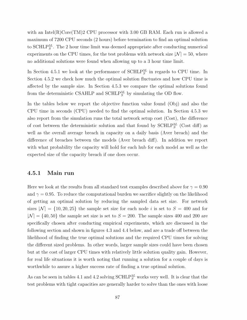
with an Intel(R)Core(TM)2 CPU processor with 3.00 GB RAM. Each run is allowed a
maximum of 7200 CPU seconds (2 hours) before termination to find an optimal solution
to SCHLP3LS . The 2 hour time limit was deemed appropriate after conducting numerical
experiments on the CPU times, for the test problems with network size |N | = 50, where
no additional solutions were found when allowing up to a 3 hour time limit.
In Section 4.5.1 we look at the performance of SCHLP3LS in regards to CPU time. In
Section 4.5.2 we check how much the optimal solution fluctuates and how CPU time is
affected by the sample size. In Section 4.5.3 we compare the optimal solutions found
from the deterministic CSAHLP and SCHLP3LS by simulating the OD flow.
In the tables below we report the objective function value found (Obj) and also the
CPU time in seconds (CPU) needed to find the optimal solution. In Section 4.5.3 we
also report from the simulation runs the total network setup cost (Cost), the difference
of cost between the deterministic solution and that found by SCHLP3LS (Cost diff) as
well as the overall average breach in capacity on a daily basis (Aver breach) and the
difference of breaches between the models (Aver breach diff). In addition we report
with what probability the capacity will hold for each hub for each model as well as the
expected size of the capacity breach if one does occur.
4.5.1 Main run
Here we look at the results from all standard test examples described above for γ = 0.90
and γ = 0.95. To reduce the computational burden we sacrifice slightly on the likelihood
of getting an optimal solution by reducing the sampled data set size. For network
sizes |N | = {10, 20, 25} the sample set size for each node i is set to S = 400 and for
|N | = {40, 50} the sample set size is set to S = 200. The sample sizes 400 and 200 are
specifically chosen after conducting empirical experiments, which are discussed in the
following section and shown in figures 4.3 and 4.4 below, and are a trade off between the
likelihood of finding the true optimal solutions and the required CPU times for solving
the different sized problems. In other words, larger sample sizes could have been chosen
but at the cost of larger CPU times with relatively little solution quality gain. However,
for real life situations it is worth noting that running a solution for a couple of days is
worthwhile to assure a higher success rate of finding a true optimal solution.
As can be seen in tables 4.1 and 4.2 solving SCHLP3LS works very well. It is clear that the
test problems with tight capacities are generally harder to solve than the ones with loose
87
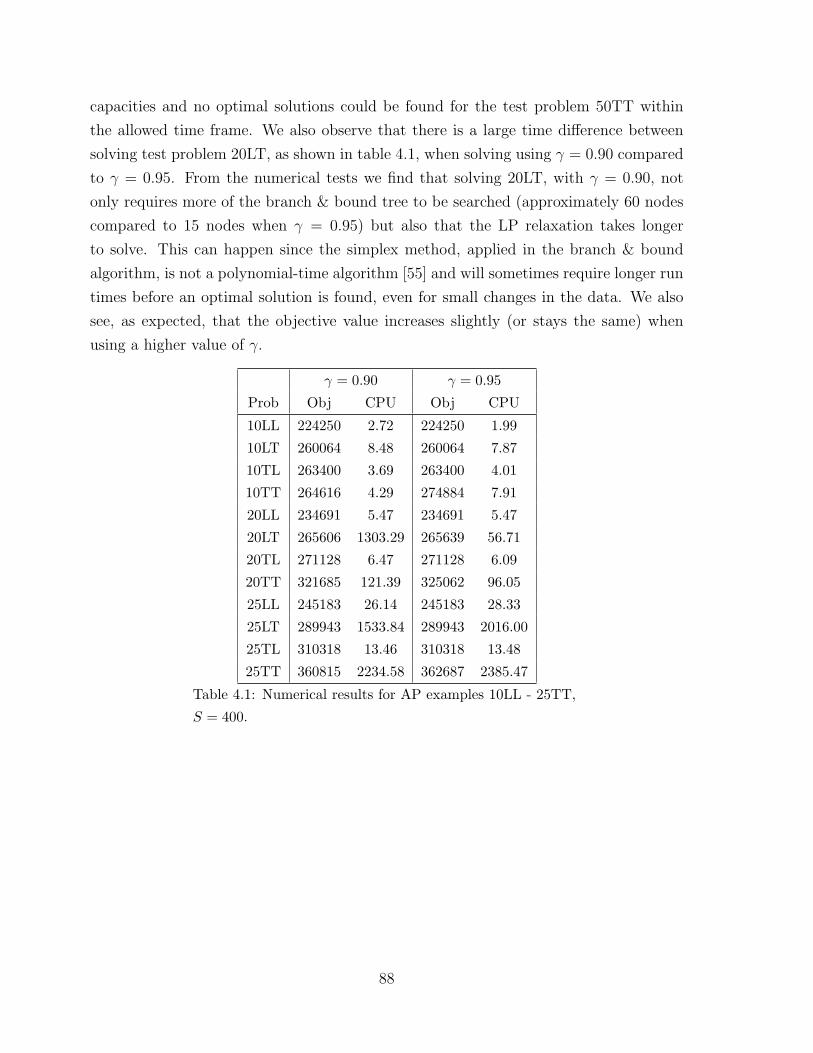
capacities and no optimal solutions could be found for the test problem 50TT within
the allowed time frame. We also observe that there is a large time difference between
solving test problem 20LT, as shown in table 4.1, when solving using γ = 0.90 compared
to γ = 0.95. From the numerical tests we find that solving 20LT, with γ = 0.90, not
only requires more of the branch & bound tree to be searched (approximately 60 nodes
compared to 15 nodes when γ = 0.95) but also that the LP relaxation takes longer
to solve. This can happen since the simplex method, applied in the branch & bound
algorithm, is not a polynomial-time algorithm [55] and will sometimes require longer run
times before an optimal solution is found, even for small changes in the data. We also
see, as expected, that the objective value increases slightly (or stays the same) when
using a higher value of γ.
γ = 0.90 γ = 0.95
Prob Obj CPU Obj CPU
10LL 224250 2.72 224250 1.99
10LT 260064 8.48 260064 7.87
10TL 263400 3.69 263400 4.01
10TT 264616 4.29 274884 7.91
20LL 234691 5.47 234691 5.47
20LT 265606 1303.29 265639 56.71
20TL 271128 6.47 271128 6.09
20TT 321685 121.39 325062 96.05
25LL 245183 26.14 245183 28.33
25LT 289943 1533.84 289943 2016.00
25TL 310318 13.46 310318 13.48
25TT 360815 2234.58 362687 2385.47
Table 4.1: Numerical results for AP examples 10LL - 25TT,
S = 400.
88

γ = 0.90 γ = 0.95
Prob Obj CPU Obj CPU
40LL 242114 56.08 242114 55.01
40LT 294407 2200.66 295251 1475.11
40TL 306461 103.47 306461 178.9
40TT 386788 5791.23 387090 1250.65
50LL 238595 289.69 239817 686.06
50LT 280582 2905.48 280582 478.79
50TL 324277 1628.93 324975 2870.41
50TT * * * *
Table 4.2: Numerical results for AP examples 40LL - 50TT,
S = 200.
4.5.2 Effects of using different sample sizes
The more data we sample in SCHLP3LS , the more hopeful we are that the location-
allocation part of the solution to this problem also solves SCHLP3. To see how sensitive
the optimal solution is in regards to the sample size we solve SCHLP3LS for the test
problems 10LT and 20TT, for sample sizes S = {100, 200, 400, 600, 800}, using γ = 0.95,
100 times each using different sampled data sets each time by applying a different seed
to the function generating the random data.
Figure 4.3: Number of times an optimal solution was found from 100 different runs for eachsample size S = {100, 200, 400, 600, 800}.
89
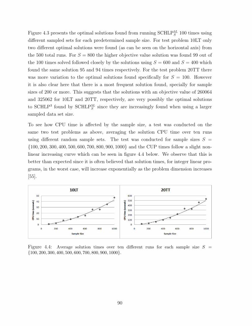
Figure 4.3 presents the optimal solutions found from running SCHLP3LS 100 times using
different sampled sets for each predetermined sample size. For test problem 10LT only
two different optimal solutions were found (as can be seen on the horizontal axis) from
the 500 total runs. For S = 800 the higher objective value solution was found 99 out of
the 100 times solved followed closely by the solutions using S = 600 and S = 400 which
found the same solution 95 and 94 times respectively. For the test problem 20TT there
was more variation to the optimal solutions found specifically for S = 100. However
it is also clear here that there is a most frequent solution found, specially for sample
sizes of 200 or more. This suggests that the solutions with an objective value of 260064
and 325062 for 10LT and 20TT, respectively, are very possibly the optimal solutions
to SCHLP3 found by SCHLP3LS since they are increasingly found when using a larger
sampled data set size.
To see how CPU time is affected by the sample size, a test was conducted on the
same two test problems as above, averaging the solution CPU time over ten runs
using different random sample sets. The test was conducted for sample sizes S =
{100, 200, 300, 400, 500, 600, 700, 800, 900, 1000} and the CUP times follow a slight non-
linear increasing curve which can be seen in figure 4.4 below. We observe that this is
better than expected since it is often believed that solution times, for integer linear pro-
grams, in the worst case, will increase exponentially as the problem dimension increases
[55].
Figure 4.4: Average solution times over ten different runs for each sample size S ={100, 200, 300, 400, 500, 600, 700, 800, 900, 1000}.
90

4.5.3 Stochastic vs. deterministic solutions
In this section we look at the difference between the optimal solutions found by the
deterministic CSAHLP and the SCHLP3LS . We solve the four different test problems
for |N | = 20. For SCHLP3LS we test both γ = 0.95 (SCHLP3L
S -0.95) and γ = 0.85
(SCHLP3LS -0.85) using a sampled set size S = 400. We then simulate the origin volumes,
Oi(ζ) at each node i, 10,000 times from the same distribution as the sampled data, i.e.
a uniform distribution between 0.5Oi and 1.5Oi, which we run on the optimal network
setups found by each model. This makes it possible to calculate the probability for a
capacity breach to occur at each hub as well as what the average size of the breach is
expected to be.
Table 4.3 presents the results of the simulations and shows what hubs were chosen (Hub),
the capacity constraint at the different chosen hubs (Capacity), the average volume of
flow arriving to each hub (Average flow), the standard deviation of the incoming flow
(S.t.d.), the probability a capacity is expected to hold for (γk = Pr[∑
iOi(ζ)Xik ≤ Γk]),
and what the expected size of the capacity breach will be if it occurs (CV aRγk =
E[∑
iOi(ζ)Xik|∑
iOi(ζ)Xik > Γk]), for each selected hub. It is clear from the runs
that when the hubs have loose (L) capacity constraints using the SCHLP3LS model to
find an optimal network setup gives limited benefits compared to using the deterministic
CSAHLP model. This is not surprising since capacities are large for the (L) capacity
constraint problems and thus capacity overruns are intrinsically unlikely. However, for
hubs which have tight (T) capacity constraints there is a huge difference. For the
test problems 20LT and 20TT, using the setup found from the deterministic model,
40%−50% of the time the volume flowing into some of the hubs will exceed hub capacity;
and on average, these breaches are 13% in excess of capacity. In contrast, capacity
breaches at the hubs using the setup found from SCHLP3LS -0.95 will at most occur 1%
of the time with, in general, a much smaller (than 13%) expected average breach size.
For SCHLP3LS -0.85, hub 14 in 20LT and hubs 10 and 19 for 20TT hold capacity 94, 94
and 96 percent of the time, respectively. These are otherwise the major problem hubs
in the deterministic model solutions as mentioned above. Although not as robust as
when using the design found from SCHLP3LS -0.95, as would be expected, it still gives
a remarkable improvement compared to the design found from the deterministic model
regarding avoidance of capacity breaches.
91
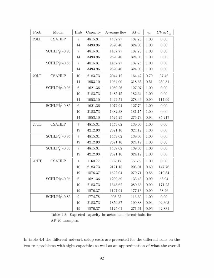
Prob Model Hub Capacity Average flow S.t.d. γk CV aRγk
20LL CSAHLP 7 4815.31 1457.77 137.78 1.00 0.00
14 3493.96 2520.40 324.03 1.00 0.00
SCHLP3LS -0.95 7 4815.31 1457.77 137.78 1.00 0.00
14 3493.96 2520.40 324.03 1.00 0.00
SCHLP3LS -0.85 7 4815.31 1457.77 137.78 1.00 0.00
14 3493.96 2520.40 324.03 1.00 0.00
20LT CSAHLP 10 2183.73 2044.12 164.42 0.79 97.46
14 1953.10 1934.00 318.65 0.51 259.81
SCHLP3LS -0.95 6 1621.36 1069.26 127.07 1.00 0.00
10 2183.73 1485.15 182.64 1.00 0.00
14 1953.10 1422.51 278.46 0.99 117.99
SCHLP3LS -0.85 6 1621.36 1072.94 127.70 1.00 0.00
10 2183.73 1382.38 181.15 1.00 0.00
14 1953.10 1524.25 276.73 0.94 85.217
20TL CSAHLP 7 4815.31 1459.02 139.03 1.00 0.00
19 4212.93 2521.16 324.12 1.00 0.00
SCHLP3LS -0.95 7 4815.31 1459.02 139.03 1.00 0.00
19 4212.93 2521.16 324.12 1.00 0.00
SCHLP3LS -0.85 7 4815.31 1459.02 139.03 1.00 0.00
19 4212.93 2521.16 324.12 1.00 0.00
20TT CSAHLP 1 1160.77 332.17 77.75 1.00 0.00
10 2183.73 2121.15 205.01 0.60 147.76
19 1576.37 1522.04 279.71 0.56 219.34
SCHLP3LS -0.95 6 1621.36 1209.59 133.43 0.99 53.94
10 2183.73 1643.62 280.63 0.99 171.25
19 1576.37 1127.94 177.13 0.99 58.26
SCHLP3LS -0.85 9 1774.78 993.55 116.30 1.00 0.00
10 2183.73 1859.37 199.88 0.94 92.303
19 1576.37 1125.01 271.61 0.96 42.831
Table 4.3: Expected capacity breaches at different hubs for
AP 20 examples.
In table 4.4 the different network setup costs are presented for the different runs on the
two test problems with tight capacities as well as an approximation of what the overall
92
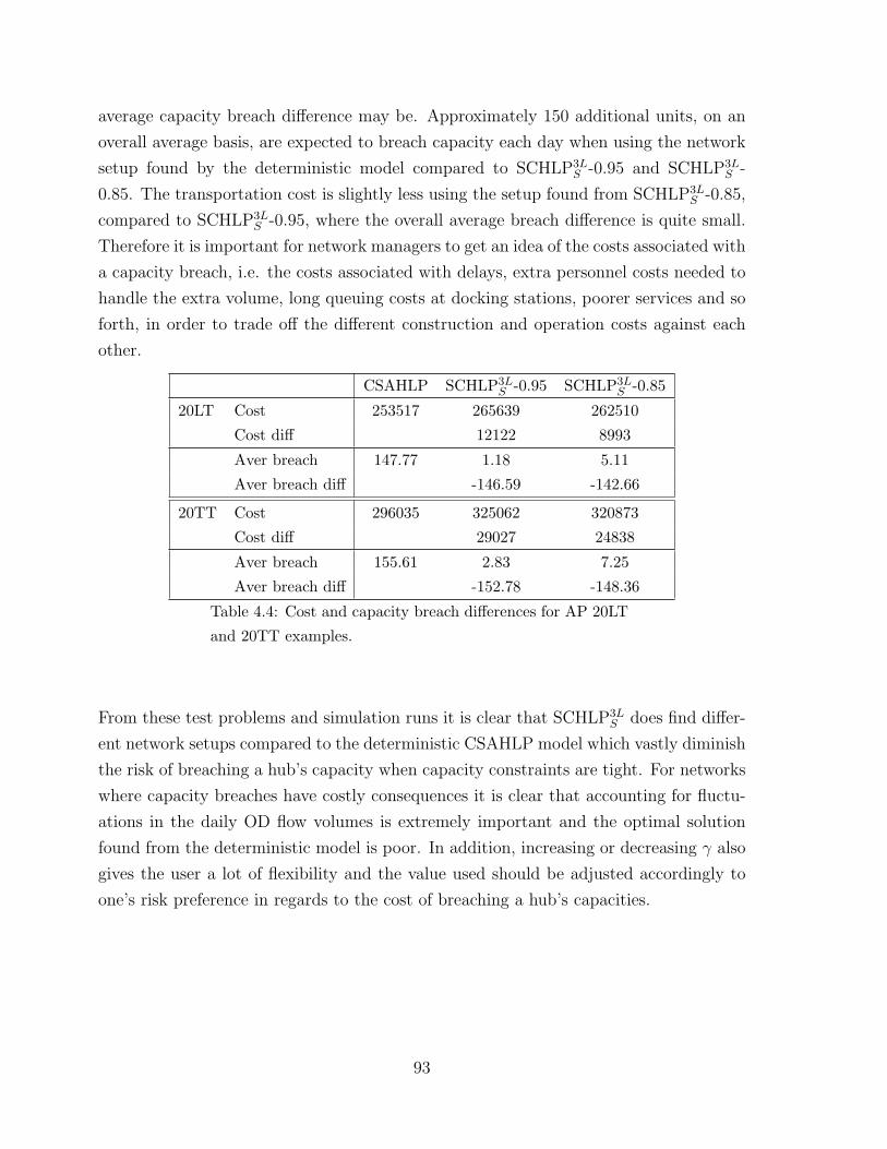
average capacity breach difference may be. Approximately 150 additional units, on an
overall average basis, are expected to breach capacity each day when using the network
setup found by the deterministic model compared to SCHLP3LS -0.95 and SCHLP3L
S -
0.85. The transportation cost is slightly less using the setup found from SCHLP3LS -0.85,
compared to SCHLP3LS -0.95, where the overall average breach difference is quite small.
Therefore it is important for network managers to get an idea of the costs associated with
a capacity breach, i.e. the costs associated with delays, extra personnel costs needed to
handle the extra volume, long queuing costs at docking stations, poorer services and so
forth, in order to trade off the different construction and operation costs against each
other.
CSAHLP SCHLP3LS -0.95 SCHLP3L
S -0.85
20LT Cost 253517 265639 262510
Cost diff 12122 8993
Aver breach 147.77 1.18 5.11
Aver breach diff -146.59 -142.66
20TT Cost 296035 325062 320873
Cost diff 29027 24838
Aver breach 155.61 2.83 7.25
Aver breach diff -152.78 -148.36
Table 4.4: Cost and capacity breach differences for AP 20LT
and 20TT examples.
From these test problems and simulation runs it is clear that SCHLP3LS does find differ-
ent network setups compared to the deterministic CSAHLP model which vastly diminish
the risk of breaching a hub’s capacity when capacity constraints are tight. For networks
where capacity breaches have costly consequences it is clear that accounting for fluctu-
ations in the daily OD flow volumes is extremely important and the optimal solution
found from the deterministic model is poor. In addition, increasing or decreasing γ also
gives the user a lot of flexibility and the value used should be adjusted accordingly to
one’s risk preference in regards to the cost of breaching a hub’s capacities.
93

4.6 Conclusion
The introduction of stochastic volume into the capacitated single allocation hub location
problem is presented and studied in this paper. The contribution of the paper is to give
better decision tools to managers when designing a hub and spoke network with capacity
constraints by being able to include the realistic and important random changes that
OD flow volumes have on a daily basis. A model with chance constraints is developed
and formulated using the risk measure conditional value-at-risk due to its effectiveness
in finding a safe value-at-risk guaranteeing that the capacity will hold with a probability
greater then or equal to γ. In addition it buffers against extreme volume increases which
can have fatal affects on a network. The model is reformulated into a strong approximate
linear formulation using sampled data, a SAA model, whose solution converges to a
solution of the original problem with probability one, exponentially fast, as the sample
size S increases. The SAA model can, in principle, be solved using any standard mixed
integer linear programing solver.
Numerical tests are conducted on the linear SAA model and show that we can solve
several test problems up to a size of 50 nodes. In addition simulation tests are carried
out and clearly show that accounting for random changes in the OD flow volumes is very
important when capacity constraints are tight as this drastically reduces the chance of
a capacity breach to occur.
94
Chapter 5
Conclusion
For transportation companies, network infrastructure and operations are critical com-
ponents which directly affect the economic health of the company. The design aspect of
a hub and spoke network for a transportation company, be it mail, cargo, air passenger
or something else, is by no means an easy or straightforward undertaking. In addition
the design aspect is not only a onetime project at the birth of the company but is an
ongoing process. For example, many post and mail companies are continuously consid-
ering how to restructure their network, in regards to number and placement of hubs,
node allocations, departure times etc., to optimize operations as demand changes over
time [1].
The academic management science and operation research hub and spoke literature aims
to help network managers, with their goal of finding an optimal hub and spoke design,
by providing new mathematical programming tools. Different modeling objectives result
in different design benefits which help different managers in different ways. Due to the
extreme complexities of finding optimal solutions to large scale systems, which consider
all parameters — dynamic, static and stochastic — and all the different variables, there
exists a gap between solvable models and the possibility of finding a real life global
optimum. Many simplified models can however still provide valuable feedback to real
life design questions. The purpose of the academic literature is not only to try to reduce
the theory practice gap but to also design simplified solvable models which still provide
valuable design suggestions.
The hub and spoke mathematical modeling literature started with one model [49], and
evolved from there. As the evolution of hub and spoke optimization started taking
95

place, heuristic algorithms, different exact solution methods and model variations began
to appear [3, 13]. This evolution is still going strong and hub and spoke modeling is now
taking steps into the world of stochastic optimization. This is an important step since
many critical network characteristics are missed when only considering averages [62].
This thesis contributes to the hub and spoke literature by being on the front line of
exploring and developing solvable models considering important stochastic processes.
The results from this thesis are very promising. For the first time exact solutions are
being found for medium sized stochastic hub and spoke problems by implementing more
efficient reformulations and solution algorithms as demonstrated in Chapter 2. Even the
approximation models in Chapters 3 and 4 seem to suggest that optimal solutions are
also possibly being found for many of the medium sized network problems. In addition,
important design questions are being answered by the solutions of these models. For
example, Chapter 3 is devoted to showing how to structure a network to be able to
provide both fast and reliable delivery services. In particular, how does one minimize
the longest path in the network so as to provide competitively fast delivery times no
matter where in the network a customer wants to ship from and to, while accounting
for the following issues: (i) random travel times for each leg as well as the random
unloading, sorting and loading times at hubs, (ii) finding and/or making sure departure
times are met even though times before everything has arrived and been loaded are
random, (iii) making sure each delivery reaches its destination node before the found
minimax time for at least some acceptable probability level γ. Also in Chapter 3, the
additional problem of maximizing the number of total packages which are delivered in
time by accounting for the costs and probabilities of late deliveries, for certain network
structures, is modeled and then solved numerically. In Chapter 4, network managers
can now find more reliable network structures that minimize costs while safely guarding
against hub capacity breaches by accounting for the daily volume fluctuations of OD
flows. In so doing, costs can be reduced by limiting the possibility of delays, extended
working hours, large queues, loss of unhappy customers, etc., due to over capacity volume
flows at hub nodes which cannot be handled efficiently. All these questions are very
important during the design phase of a hub and spoke network and solutions are now
available to find where important real life stochastic processes are considered.
It is important to note however, that cost and time minimizations don’t always go hand
in hand and each network manager will have to weigh one against the other depending
upon capital and operational budgets, existing competition and type of service. The
service cost model, presented in Chapter 3, is however a promising type of hybrid where
96

costs of missed delivery times are considered. More on this together with some future
research suggestions are discussed in the following section.
5.1 Future Research
The hope is that future research will continue developing stochastic optimization models
and methods building on, among others, the model designs and methodologies presented
in the preceding chapters. The well known question, which is of great practical impor-
tance, of how to deal with the dual, and often opposing, objective functions of mini-
mizing delivery times and network costs simultaneously, is an important future research
question. The service cost problem, introduced in Chapter 3, has great potential as a
stepping stone to solving this problem. As mentioned, it is a type of hybrid model which
considers the cost of missed delivery times and can therefore more easily be extended to
account for the total network costs, as opposed to a center type problem where travel
time has no direct network cost relationship. This would be both a very intriguing and
important future research question to consider while keeping the stochastic travel time
properties and incorporating stochastic demand if capacity constraints are present. How-
ever, prior to this step it may be well worth first looking into and developing appropriate
formulations and solution algorithms to solving the location-allocation problem, for both
variable and fixed departure times applied on the service cost problem. Additionally,
research on how to account for stochastic OD flow volumes and looking into how/if this
can affect the probability of a path making it on time, due to possible congestion at
hub nodes on high volume days, for the service cost problem, is important. Finding
efficient models and solution methods for these questions would be a major contribution
and very beneficial to network managers. They would have tools which would allow
optimal or near optimal solutions to be found while accounting for important real life
system components such as increasing the probability of goods being delivered on time,
accounting for departure times at hub nodes, considering stochastic network effects on
the demand and travel times, while all at the same time minimizing the overall network
costs.
An alternative approach to the dual objective function problem discussed above is to
add probabilistic time constraints to the stochastic hub location problem presented in
Chapter 4. This would not account for the costs of missed deliveries but would minimize
the costs associated with the network setup while guarding against capacity constraint
97
violations while at the same time guaranteeing delivery time services. In addition,
one could further look into whether the stochastic travel times of arriving goods into
a hub are affecting the congestion at each hub node in a positive or a negative way.
Understanding this and developing efficient models and solution methods would be of
great value for network system designers.
Another important future research question is in regards to the new stochastic p-hub
center problems also introduced in Chapter 3. The two different departure time models
presented in Chapter 3 are appropriate and of great importance for delivery companies,
however, the models could further be developed to better fit airline passenger hub and
spoke systems where an airline company may have multiple slot time departure options
to choose from for all hub-hub links. The second model presented in Chapter 3 can
handle some departure time options but would explode in size if multiple options were
available for every hub-hub link, which may be the case for some airline companies.
Developing this would therefore be a very beneficial research question.
Several other interesting research questions exist such as modelling a robust approach
for handling uncertainty environments for the center, covering and median type prob-
lems while incorporating hub departure times. Accounting for risk or uncertainty in a
competitive environment where one considers the actions of competing players in the
system would also be an interesting and important question. This would bring game the-
ory into the stochastic hub and spoke literature as well. Lastly, looking into additional
improvements of existing models, to be able to solve even larger networks, is always a
sought after and appreciated research question.
Thus it is clear that there are many interesting future research areas for stochastic
optimization, and we hope to see at least some of them taken up in the future. Only
in this way will the field continue to develop. The very human nature of wanting to
explore, improve, understand and find solutions is what makes us great and allows us
to grow as a species. If a person can answer just a single research question, it will mean
the world, since only then can we keep developing. “Almost everything you do will seem
insignificant, but it is important that you do it” — Gandhi.
98

Bibliography
[1] Personal communication, National postal company, Europe, 2009.
[2] M. Albareda-Sambola, E. Fernndez, and F. S. da Gama. The facility location
problem with Bernoulli demands. Omega, 39(3):335 – 345, 2011.
[3] S. Alumur and B. Y. Kara. Network hub location problems: The state of the art.
European Journal of Operational Research, 190(1):1–21, 2008.
[4] F. Andersson, H. Mausser, D. Rosen, and S. Uryasev. Credit risk optimization
with conditional value-at-risk criterion. Mathematical Programming, 89(2):273–291,
2001.
[5] J. Atlason, M. Epelman, and S. Henderson. Call center staffing with simulation
and cutting plane methods. Annals of Operations Research, 127:333–358, 2004.
[6] T. Aykin. On ‘A quadratic integer program for the location of interacting hub
facilities’. European Journal of Operational Research, 46:409–411, 1990.
[7] O. Baron, O. Berman, and D. Krass. Facility location with stochastic demand and
constraints on waiting time. Manufacturing & Service Operations Management,
10:484–505, 2008.
[8] N. Boysen, M. Fliedner, and A. Scholl. Scheduling inbound and outbound trucks
at cross docking terminals. OR Spectrum, 32:135–161, 2010.
[9] J. F. Campbell. Location and allocation for distribution systems with transship-
ments and transportation economies of scale. Annals of Operations Research, 40:77–
99, 1992.
[10] J. F. Campbell. Integer programming formulations of discrete hub location prob-
lems. European Journal of Operational Research, 72:387–405, 1994.
99
[11] J. F. Campbell. Integer programming formulations of discrete hub location prob-
lems. European Journal of Operational Research, 72:387–405, 1994.
[12] J. F. Campbell. Hub location and the p-hub median problem. Operations Research,
44(6):923–935, 1996.
[13] J. F. Campbell, A. Ernst, and M. Krishnamoorthy. Hub location problems. In
H. Hamacher and Z. Drezner, editors, Location Theory: Applications and Theory,
pages 373–406. Springer-Verlag, 2001.
[14] R. Carbone. Public facilities location under stochastic demand. ONFOR, 12:261–
270, 1974.
[15] I. Contreras, J.-F. Cordeau, and G. Laporte. Stochastic uncapacitated hub loca-
tion. HEC Montreal and Interuniversity Research Centre on Enterprise Networks,
Logistics and Transportation (CIRRELT), Montreal, Canada, 2010.
[16] I. Contreras, J. A. Diaz, and E. Fernandez. Branch-and-price for large-scale ca-
pacitated hub location problems with single assignment. INFORMS Journal on
Computing, 23:41–55, 2011.
[17] I. Correia, S. Nickel, and F. S. da Gama. The capacitated single-allocation hub
location problem revisited: A note on a classical formulation. European Journal of
Operational Research, 207:92–96, 2010.
[18] M. da Graca Costa, M. E. Captivo, and J. Climaco. Capacitated single allocation
hub location problem - a bi-criteria approach. Computers & Operations Research,
35:3671–3695, 2008.
[19] L. Dai, C. H. Chen, and J. R. Birge. Convergence properties of two-stage stochastic
programming. Journal of Optimization Theory and Applications, 106(3):489–509,
2000.
[20] R. S. de Camargo, G. Miranda, and H. P. Luna. Benders decomposition for the
uncapacitated multiple allocation hub location problem. Computers & Operations
Research, 35(4):1047–1064, 2008.
[21] U. Dorndorf, A. Drexl, Y. Nikulin, and E. Pesch. Flight gate scheduling: State-of-
the-art and recent developments. Omega, 35:326–334, 2007.
100

[22] J. Ebery. Solving large single allocation p-hub location problems with 2 or 3 hubs.
European Journal of Operational Research, 128(2):447–458, 2001.
[23] S. Elhedhli and F. X. Hu. Hub-and-spoke network design with congestion. Com-
puters & Operations Research, 32:1615–1632, 2005.
[24] A. T. Ernst, H. Hamacher, H. Jiang, M. Krishnamoorthy, and G. Woeginger. Un-
capacitated single and multiple allocation p-hub center problems. Computers &
Operations Research, 36(7):2230–2241, 2009.
[25] A. T. Ernst and M. Krishnamoorthy. Efficient algorithms for the uncapacitated
single allocation p-hub median problem. Location Science, 4:139–154, 1996.
[26] A. T. Ernst and M. Krishnamoorthy. Exact and heuristic algorithms for the unca-
pacitated multiple allocation p-hub median problem. European Journal of Opera-
tional Research, 104(1):100–112, 1998.
[27] A. T. Ernst and M. Krishnamoorthy. An exact solution approach based on shortest-
paths for p-hub median problems. INFORMS Journal on Computing, 10(2):149–
162, 1998.
[28] A. T. Ernst and M. Krishnamoorthy. Solution algorithms for the capacitated single
allocation hub location problem. Annals of Operations Research, 86:141–159, 1999.
[29] A. S. Fotheringham. A new set of spatial interaction models: The theory of com-
peting destinations. Environment and Planning A, pages 15–36, 1983.
[30] O. Garnett, A. Mandelbaum, and M. Reiman. Designing a call center with impa-
tient customers. Manufacturing and Service Operations Management, 4(3):208–227,
2002.
[31] G. Ghiani, F. Guerriero, G. Laporte, and R. Musmanno. Real-time vehicle routing:
Solution concepts, algorithms and parallel computing strategies. European Journal
of Operational Research, 151:1–11, 2003.
[32] I. Gurvich, M. Armony, and A. Mandelbaum. Service-level differentiation in call
centers with fully flexible servers. Management Science, 54(2):279–294, 2008.
[33] E. Hult, H. Jiang, and D. Ralph. Exact computational approaches to a stochas-
tic uncapacitated single allocation p-hub center problem. Judge Business School,
University of Cambridge, Trumpington Street, Cambridge, United Kingdom, 2011.
101
[34] E. L. Johnson, G. L. Nemhauser, and M. W. Savelsbergh. Progress in linear
programming-based algorithms for integer programming: An exposition. INFORMS
Journal on Computing, 12(1):2–23, 2000.
[35] P. Jorion. Value at Risk: The new benchmark for managing financial risk. The
McGraw-Hill Companies, Inc., 2007.
[36] S. Juette, O. Gavriliouk, and H. Hamacher. Polyhedral analysis of uncapacitated
single allocation p-hub center problems. Technical Report 109, FB Mathematik,
TU Kaiserslautern, 2007.
[37] B. Y. Kara and B. C. Tansel. On the single-assignment p-hub center problem.
European Journal of Operational Research, 125(3):648–655, 2000.
[38] B. Y. Kara and B. C. Tansel. The latest arrival hub location problem. Management
Science, 47(10):1408–1420, 2001.
[39] A. Kleywegt, A. Shapiro, and T. Homen-De-Mello. The sample average approxima-
tion method for stochastic discrete optimization. SIAM Journal on Optimization,
12(2):479–502, 2001.
[40] J. G. Klincewicz. Heuristics for the p-hub location problem. European Journal of
Operational Research, 53(1):25–37, 1991.
[41] J. G. Klincewicz. Avoiding local optima in the p-hub location problem using tabu
search and grasp. Annals of Operations Research, 40:283–302, 1992.
[42] P. Krokhmal, J. Palmquist, and S. Uryasev. Portfolio optimization with conditional
value-at-risk objective and constraints. Journal of Risk, 4(2):43–68, 2002.
[43] F. Y. Louveaux. Discrete stochastic location models. Annals of Operations Re-
search, 6:23–34, 1986.
[44] V. Marianov and D. Serra. Location models for airline hubs behaving as M/D/c
queues. Computers & Operations Research, 30:983–1003, 2003.
[45] V. Marianov, D. Serra, and C. ReVelle. Location of hubs in a competitive environ-
ment. European Journal of Operational Research, 114:363–371, 1999.
[46] H. M. Markowitz. Portfolio selection. The Journal of Finance, 7:77–91, 1952.
102

[47] J. C. Martin and C. Roman. Hub location in the South-Atlantic airline market: A
spatial competition game. Transportation Research Part A, pages 865–888, 2003.
[48] T. Meyer, A. T. Ernst, and M. Krishnamoorthy. A 2-phase algorithm for solving
the single allocation p-hub center problem. Computers & Operations Research,
36(12):3143–3151, 2009.
[49] M. E. O’Kelly. A quadratic integer program for the location of interacting hub
facilities. European Journal of Operational Research, 32:393–404, 1987.
[50] M. E. O’Kelly. Hub facility location with fixed costs. Papers in Regional Science:
The Journal of the RSAI, 71:293–306, 1992.
[51] M. E. O’Kelly. Routing traffic at hub facilities. Networks and Spatial Economics,
10(2):173–191, 2010.
[52] M. E. O’Kelly, D. Bryan, D. Skorin-Kapov, and J. Skorin-Kapov. Hub network de-
sign with single and multiple allocation: A computational study. Location Science,
4(3):125–138, 1996.
[53] M. E. O’Kelly, D. Skorin-Kapov, and J. Skorin-Kapov. Lower bounds for the hub
location problem. Management Science, 41(4):713–721, 1995.
[54] P. Pamuk and C. Sepil. A solution to the hub center problem via a single-relocation
algorithm with tabu search. IEE Transactions, 33:399–411, 2001.
[55] C. H. Papadimitriou and K. Steiglitz. Combinatorial Optimization Algorithms and
Complexity. Dover Publications, Inc., 1998.
[56] H. Pirkul and D. A. Schilling. An efficient procedure for designing single allocation
hub and spoke systems. Management Science, 44(12):S235–S242, 1998.
[57] R. T. Rockafellar and S. Uryasev. Optimization of conditional value-at-risk. The
Journal of Risk, 2(3), 2000.
[58] R. T. Rockafellar and S. Uryasev. Conditional value-at-risk for general loss distri-
butions. Journal of Banking & Finance, 26:1443–1471, 2002.
[59] J. Rosenhead, M. Elton, and S. Gupta. Robustness and optimality as criteria for
strategic decisions. Operational Research Quarterly (1970-1977), 23(4):413–431,
1972.
103

[60] H. W. Samir Elhedhli. A Lagrangean heuristic for hub-and-spoke system design
with capacity selection and congestion. INFORMS Journal on Computing, 22:282–
296, 2010.
[61] M. Sasaki. Hub network design model in a competitive environment with flow
threshold. Journal of the Operations Research Society of Japan, 48:158–171, 2005.
[62] S. Savage. Decision Making with Insight. Duxbury Press, 2003.
[63] S. Savage. Flaw of averages. San Jose Mercury News, 2008.
[64] E. Sheppard. A conceptual framework for dynamic location-allocation analysis.
Environment and Planning A, 6:547–564, 1974.
[65] T. Sim, T. Lowe, and B. Thomas. The stochastic p-hub center problem with service-
level constraints. Computers & Operations Research, 36:3166–3177, 2009.
[66] D. Skorin-Kapov and J. Skorin-Kapov. On tabu search for the location of interacting
hub facilities. European Journal of Operational Research, 73:502–509, 1994.
[67] D. Skorin-Kapov, J. Skorin-Kapov, and M. E. O’Kelly. Tight linear programming
relaxations of uncapacitated p-hub median problems. European Journal of Opera-
tional Research, 94:582–593, 1996.
[68] K. Smith, M. Krishnamoorthy, and M. Palaniswami. Neural versus traditional
approaches to the location of interacting hub facilities. Location Science, 4:155–
171, 1996.
[69] L. V. Snyder. Facility location under uncertainty: a review. IIE Transactions,
38:537–554, 2006.
[70] J. Sohn and S. Park. A linear program for the two-hub location problem. European
Journal of Operational Research, 100(3):617–622, 1997.
[71] J. Sohn and S. Park. Efficient solution procedure and reduced size formulations for
p-hub location problems. European Journal of Operational Research, 108(1):118–
126, 1998.
[72] J. Sohn and S. Park. The single allocation problem in the interacting three hub
network. Networks, 35:17–25, 2000.
104

[73] D. Steenken, S. Voss, and R. Stahlbock. Container terminal operation and op-
erations research - a classification and literature review. OR Spectrum, 26:3–49,
2004.
[74] B. Wagner. A note on ‘the latest arrival hub location problem’. Management
Science, 50:1751–1752, 2004.
[75] M. R. Wagner, J. Bhadury, and S. Peng. Risk management in uncapacitated fa-
cility location models with random demands. Computers & Operations Research,
36:1002–1011, 2009.
[76] J. Wang. The β-reliable median on a network with discrete probabilistic demand
weights. Operations Research, 55:966–975, 2007.
[77] W. Wang and S. Ahmed. Sample average approximation of expected value con-
strained stochastic programs. Operations Research Letters, 36:515–519, 2008.
[78] J. R. Weaver and R. L. Church. Computational procedures for location problems
on stochastic networks. Transportation Science, 17:168–180, 1983.
[79] M. Wen and K. Iwamura. Fuzzy facility location-allocation problem under the
Hurwicz criterion. European Journal of Operational Research, 184:627–635, 2008.
[80] H. Yaman, B. Kara, and B. Tansel. The latest arrival hub location problem for cargo
delivery systems with stopovers. Transportation Research Part B, 41(8):906–919,
2007.
[81] T.-H. Yang. Stochastic air freight hub location and flight routes planning. Applied
Mathematical Modelling, 33:4424–4430, 2009.
[82] W. Yu. Operational strategies for cross docking systems. Iowa State University,
Ph.D. Dissertation, 2002.
[83] J. Zhou and B. Liu. New stochastic models for capacitated location-allocation
problem. Computers & Industrial Engineering, 45:111–125, 2003.
105