Embed Size (px)
Citation preview
1
PhD Thesis
ASSESSING PROCESS DESIGN WITH REGARD TO MPC PERFORMANCE USING A NOVEL
MULTI-MODEL PREDICTION METHOD
Flavio A. M. Strutzel
Supervisor:
I. David L. Bogle
21st November 2017

Declaration
2
Declaration
I, Flavio Augusto Martins Strutzel, confirm that the work presented in this Thesis is
my own. Where information has been derived from other sources, I confirm that this has
been indicated in the Thesis.
Signature:____________________________
Date: 21/11/2017
3
Abstract
Model Predictive Control (MPC) is nowadays ubiquitous in the chemical industry
and offers significant advantages over standard feedback controllers. Notwithstanding,
projects of new plants are still being carried out without assessing how key design
decisions, e.g., selection of production route, plant layout and equipment, will affect
future MPC performance. The problem addressed in this Thesis is comparing the
economic benefits available for different flowsheets through the use of MPC, and thus
determining if certain design choices favour or hinder expected profitability. The
Economic MPC Optimisation (EMOP) index is presented to measure how disturbances
and restrictions affect the MPC’s ability to deliver better control and optimisation.
To the author’s knowledge, the EMOP index is the first integrated design and control
methodology to address the problem of zone constrained MPC with economic
optimisation capabilities (today's standard in the chemical industry). This approach
assumes the availability of a set of linear state-space models valid within the desired
control zone, which is defined by the upper and lower bounds of each controlled and
manipulated variable. Process economics provides the basis for the analysis. The index
needs to be minimised in order to find the most profitable steady state within the zone
constraints towards which the MPC is expected to direct the process. An analysis of the
effects of disturbances on the index illustrates how they may reduce profitability by
restricting the ability of an MPC to reach dynamic equilibrium near process constraints,
which in turn increases product quality giveaway and costs. Hence the index monetises
the required control effort.
Since linear models were used to predict the dynamic behaviour of chemical
processes, which often exhibit significant nonlinearity, this Thesis also includes a new
multi-model prediction method. This new method, called Simultaneous Multi-Linear
Prediction (SMLP), presents a more accurate output prediction than the use of single
linear models, keeping at the same time much of their numerical advantages and their
relative ease of obtainment. Comparing the SMLP to existing multi-model approaches,
the main novelty is that it is built by defining and updating multiple states simultaneously,
thus eliminating the need for partitioning the state-input space into regions and
Abstract
4
associating with each region a different state update equation. Each state’s contribution
to the overall output is obtained according to the relative distance between their
identification point, i.e., the set of operating conditions at which an approximation of the
nonlinear model is obtained, and the current operating point, in addition to a set of
parameters obtained through regression analysis.
Additionally, the SMLP is built upon data obtained from step response models that
can be obtained by commercial, black-box dynamic simulators. These state-of-the-art
simulators are the industry’s standard for designing large-scale plants, the focus of this
Thesis. Building an SMLP system yields an approximation of the nonlinear model, whose
full set of equations is not of the user’s knowledge. The resulting system can be used for
predictive control schemes or integrated process design and control. Applying the SMLP
to optimisation problems with linear restrictions results in convex problems that are easy
to solve. The issue of model uncertainty was also addressed for the EMOP index and
SMLP systems. Due to the impact of uncertainty, the index may be defined as a numeric
interval instead of a single number, within which the true value lies.
A case of study consisting of four alternative designs for a realistically sized crude
oil atmospheric distillation plant is provided in order to demonstrate the joint use and
applicability of both the EMOP index and the SMLP. In addition, a comparison between
the EMOP index and a competing methodology is presented that is based on a case study
consisting of the activated sludge process of a wastewater treatment plant.
Keywords
Integrated Process Design and Control, Simultaneous Process Design and Control,
Model Predictive Control, MPC, Zone Constrained MPC, Zone Control, Controllability
Analysis, Crude Oil Distillation, Linear Hybrid Systems, Multi-model MPC, Activated
Sludge Wastewater Treatment.
Impact Statement
5
Impact Statement
This Thesis presents two main novel elements: a new integrated process design and
control approach; and a new method for approximating nonlinear systems as a collection
of linear state-space models.
The first contribution, called EMOP index methodology, can be used as a decision-
making tool during the design phase of new chemical, petrochemical and oil refining
units. It provides a performance ranking of candidate designs based on their expected
operating expenses (OPEX) in a number of production scenarios. The main case study
presented in this Thesis, which studied realistic designs for a crude oil distillation unit,
demonstrated that the selection of a suboptimal flowsheet can increase OPEX from 2%
to 55% relative to the optimal flowsheet. Even the lower range of this figure translates
into expressive amounts of money being wasted, especially given the long life-cycles of
the chemical industry’s projects. Design teams working for project companies or their
clients should apply the EMOP index because it is the first Controllability Analysis
method adequate for the special case of zone constrained model predictive control (MPC),
the chemical industry’s de facto standard for advanced control systems. Also, like any
method of Controllability Analysis, the EMOP index can be used to discover serious
controllability issues in the early design phase, which has the potential of saving millions
of dollars by avoiding delays in the project completion to implement corrections, or
avoiding a lifetime of troubled operation, if corrections are not implemented. Unlike most
methods, however, EMOP can provide an estimative for the losses such controllability
issues can create. Inside academia, this work can have an impact by inspiring research on
new methods for zone constrained MPC, as well as new efforts to monetise
controllability.
The second contribution is a linear state-space formulation capable of accurately
representing inherently nonlinear processes without incurring in the mathematical
disadvantages of using nonlinear models. Called Simultaneous Multi-Linear Prediction
(SMLP), this formulation can be applied with MPC, yielding more precise control actions
by reducing the prediction error. Nonetheless, the advantage of providing a better
approximation of nonlinear models is even more relevant when the prediction is used for
integrated process design and control. In this field, even small accuracy gains are

Impact Statement
6
extremely important and may impact the layout choice for a new plant. A comparison
between a PieceWise Affine system (a standard multi-model formulation) and the SMLP
showed that the later provided an accuracy gain of 44.86%, using the nonlinear model as
a reference. Another advantage is the economy of both computational time and
engineering man-hours required as compared to developing a nonlinear, rigorous first-
principles or hybrid model for a complex industrial process. SMLP may inspire further
developments in the Linear Hybrid Systems framework, and automation suppliers may
embed SMLP in their MPC solutions.

Acknowledgements
7
Acknowledgements
I thank CAPES and Brazil’s ministry of education for the financial support and
scholarship. I appreciate the confidence placed in me by the Brazilian Government.
I thank Prof David Bogle for his support and advice. His contribution to this Thesis
was invaluable.
I thank parents Marcos and Jane, my brothers Sergio and Fernando and all my family
for the love, support and patience without which nothing would this project would never
have taken place.
I thank Petrobras Company and the University of Sao Paulo for the encouragement
and training as an engineer in my formative years. Special thanks go to the engineers
Oswaldo Luiz Carrapiço, Antonio Carlos Zanin, and Prof Darci Odloak.
I thank University College London for the excellent environment, the guidance and
the opportunity.
8
Table of Contents
Declaration ........................................................................................................................ 2
Abstract ............................................................................................................................. 3
Impact Statement ............................................................................................................... 5
Acknowledgements ........................................................................................................... 7
Table of Contents ............................................................................................................. 8
Notation List ................................................................................................................... 11
Acronyms List ................................................................................................................. 20
List of Figures ................................................................................................................. 22
List of Tables................................................................................................................... 24
1 Introduction and Motivation .................................................................................... 26
1.1 The Integrated Process Design and Control Framework .................................. 26
1.2 A Classification for Integrated Process Design and Control Methods ............. 28
1.3 Model Predictive Control and the Monetisation of Control Performance ....... 30
1.4 Project Motivation ............................................................................................ 33
1.5 Thesis Organisation .......................................................................................... 35
2 Literature Review .................................................................................................... 37
2.1 Review of Integrated Process and Control Design Methodologies .................. 37
5. Review of Integrated Process Design and Model Predictive Control .................. 37
2.1.1 Concepts and Measures of Controllability ................................................ 38
2.1.2 Process-Oriented Methods for Controllability Analysis ........................... 56
2.1.3 Integrated Process Design and Control Framework - Methods of
Integrated Control and Process Synthesis ................................................................ 62
2.1.4 Conclusions from the Review of Integrated Process Design and Control
Framework ............................................................................................................... 76
2.2 Review of Model Predictive Control ................................................................ 77
2.2.1 Robust Model Predictive Control and Techniques to Enforce Stability ... 80
2.2.2 Zone Constrained Model Predictive Control ............................................ 83
2.2.3 Interfaces of industrial MPC implementations ......................................... 87
2.2.4 Conclusions from the Model Predictive Control Review ......................... 88
Table of Contents
9
2.3 Review of Integrated Process Design and Model Predictive Control
Methodologies ............................................................................................................. 88
2.3.1 Embedding MPC in Flowsheet Analysis .................................................. 89
2.3.2 Conclusions from the review of integrated process design and MPC
methodologies .......................................................................................................... 95
2.4 The Linear Hybrid Systems framework ........................................................... 98
2.5 Conclusions from the Literature Review ........................................................ 101
3 Assessing Plant Design for MPC Performance ..................................................... 102
3.1 A State-Space Methodology ........................................................................... 109
3.2 Index for Control Bound Violations ............................................................... 111
3.3 An Economic Optimisation Index .................................................................. 112
3.4 The Simplified Economic MPC Optimisation Index (EMOP) ...................... 114
3.5 Ensuring Viable Solutions .............................................................................. 116
3.6 EMOP Index Interpretation and Tuning ......................................................... 120
3.7 Including price variations in the EMOP cost function ................................... 122
3.8 Exploring the Relation between the Regulatory Control Layer, MPC Layer and
the EMOP Index ........................................................................................................ 123
3.9 Using the EMOP index to compare plants with radically different layouts ... 125
3.10 Conclusions concerning the EMOP index ...................................................... 128
4 The simultaneous multi-linear prediction .............................................................. 130
4.1.1 Generating sub-models............................................................................ 132
4.1.2 Introducing the Simultaneous Multi-Linear Prediction (SMLP) ............ 133
4.1.3 SMLP Method 1 – the MIMO parametrisation ....................................... 134
4.1.4 SMLP Method 2 – Operating point (OP) defined as the input vector .... 143
4.1.5 SMLP Method 3 – the SISO parametrisation ......................................... 144
4.1.6 The stability of an SMLP system ............................................................ 148
4.1.7 Reachability of an SMLP system ............................................................ 149
4.1.8 Filtering sub-state changes ...................................................................... 150
5 Quantifying the effects of model uncertainty in the joint use of the EMOP index
and the SMLP ................................................................................................................ 151
5.1.1 An alternative method to modelling uncertainty – the model identification
error-based approach.............................................................................................. 160
6 Case of Study - EMOP Index for an Oil Distillation Process Unit........................ 163
6.1 Describing the Control Problem ..................................................................... 163
6.2 Measuring the Economic Impact of the Control Effort .................................. 167
6.3 Defining parameters for the measurement of a monetised control cost ......... 168
Table of Contents
10
6.4 Results and Discussion ................................................................................... 172
6.4.1 Applying the SMLP approach for the Crude Oil distillation .................. 173
6.4.2 Scenario 1 – Simultaneous control and optimisation while handling a
measured disturbance ............................................................................................. 175
6.4.3 Scenario 2 – Price changes ...................................................................... 177
6.4.4 Selecting the Best Plant ........................................................................... 179
6.4.5 Effect of Soft-Landing matrices and error penalization matrices ........... 180
6.4.6 Optimisation algorithm and computational cost ..................................... 181
6.4.7 Model uncertainty - obtaining a EMOP index interval for one of the
designs 182
6.4.8 Conclusions from the Crude Oil Distillation Study Case ....................... 184
7 Comparison between two Integrated Process Design and Control Methodologies
186
7.1 Description of an Activated Sludge Wastewater Treatment Plant ................. 187
7.1.1 Mathematical model of the ASP for substrate removal .......................... 187
7.1.2 Results from the Integrated Design (ID) Methodology (Francisco et al.,
2011) 191
7.1.3 Nonlinear State-Space Model for the ASP.............................................. 193
7.1.4 Applying the Economic MPC Optimisation index to the ASP ............... 196
7.1.5 Computational cost of the ASP case study ............................................. 199
7.2 Using the ASP as a case study to benchmark the Simultaneous Multi-Linear
Prediction (SMLP) .................................................................................................... 199
7.2.1 A linearised state-space model for the ASP ............................................ 200
7.2.2 PWA and SMLP representations of the ASP .......................................... 202
7.2.3 Comparison of results ............................................................................. 203
7.3 Final considerations about the Simultaneous Multi-Linear Prediction method
205
8 Conclusions ............................................................................................................ 207
References ..................................................................................................................... 210
Appendix ....................................................................................................................... 224
Notation List
11
Notation List
Roman alphabet
Symbol Definition Unit
������ State-space disturbance matrix along the prediction horizon
������ State-space input matrix along the control horizon
��� Target for state change of the subsystem ϑ
� Target for state change of the SMLP system
�,� Initial state of the subsystem ϑ
�, Target state of the subsystem ϑ
����� average value of the CV with quality threshold through the
prediction horizon
������ Value of CV quality threshold value for which the price
variation occurs
��� State-space model system matrix of sub-model ϑ
�� Settler area m�
��� State-space model input matrix of sub-model ϑ
��� State-space model output matrix of sub-model ϑ
�� Dissolved oxygen (DO) concentration at the output of the
aeration tanks input flow mg/L
�� Saturation oxygen (DO) concentration in the aeration tanks ���
�� State-space model disturbance matrix of sub-model ϑ
! Space of possible disturbance values
�� Measured vector of disturbance variables (DVs)
"�#$ Absolute value of prediction error of sub-model ϑ relative to
step n
&',( Error relative to controlled variable i at each instant k
&)'*$ Linearisation error for a single sub-model ϑ
+(� Aeration factor
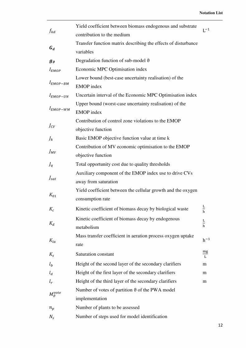
Notation List
12
+(, Yield coefficient between biomass endogenous and substrate
contribution to the medium L.�
/� Transfer function matrix describing the effects of disturbance
variables
0� Degradation function of sub-model ϑ
23456 Economic MPC Optimisation index
23456.74 Lower bound (best-case uncertainty realisation) of the
EMOP index
23456.89 Uncertain interval of the Economic MPC Optimisation index
23456.:4 Upper bound (worst-case uncertainty realisation) of the
EMOP index
;<= Contribution of control zone violations to the EMOP
objective function
;( Basic EMOP objective function value at time k
;4= Contribution of MV economic optimisation to the EMOP
objective function
;> Total opportunity cost due to quality thresholds
;�?@ Auxiliary component of the EMOP index use to drive CVs
away from saturation
AB� Yield coefficient between the cellular growth and the oxygen
consumption rate
AC Kinetic coefficient of biomass decay by biological waste �D
A, Kinetic coefficient of biomass decay by endogenous
metabolism
�D
A)? Mass transfer coefficient in aeration process oxygen uptake
rate h.�
A� Saturation constant ���
FG Height of the second layer of the secondary clarifiers m
F, Height of the first layer of the secondary clarifiers m
FH Height of the third layer of the secondary clarifiers m
I$JK@L Number of votes of partition ϑ of the PWA model
implementation
MN Number of plants to be assessed
O� Number of steps used for model identification
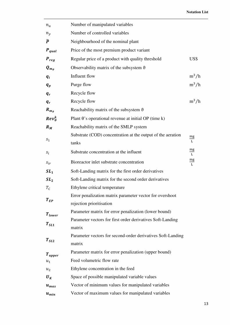
Notation List
13
MP Number of manipulated variables
MQ Number of controlled variables
RS Neighbourhood of the nominal plant
R���� Price of the most premium product variant
RT�0 Regular price of a product with quality threshold US$
U�� Observability matrix of the subsystem ϑ
�V Influent flow mW h⁄
�Y Purge flow mW h⁄
�T Recycle flow
�T Recycle flow mW h⁄
Z�� Reachability matrix of the subsystem ϑ
Z��[\ Plant θ’s operational revenue at initial OP (time k)
Z Reachability matrix of the SMLP system
^� Substrate (COD) concentration at the output of the aeration
tanks
���
^' Substrate concentration at the influent ���
^'H Bioreactor inlet substrate concentration ���
_`� Soft-Landing matrix for the first order derivatives
_` Soft-Landing matrix for the second order derivatives
a< Ethylene critical temperature
bcR Error penalization matrix parameter vector for overshoot
rejection prioritisation
b�de�T Parameter matrix for error penalization (lower bound)
b_`� Parameter vectors for first order derivatives Soft-Landing
matrix
b_` Parameter vectors for second-order derivatives Soft-Landing
matrix
b�YY�T Parameter matrix for error penalization (upper bound)
f� Feed volumetric flow rate
f� Ethylene concentration in the feed
g! Space of possible manipulated variable values
��� Vector of minimum values for manipulated variables
��Vh Vector of maximum values for manipulated variables
Notation List
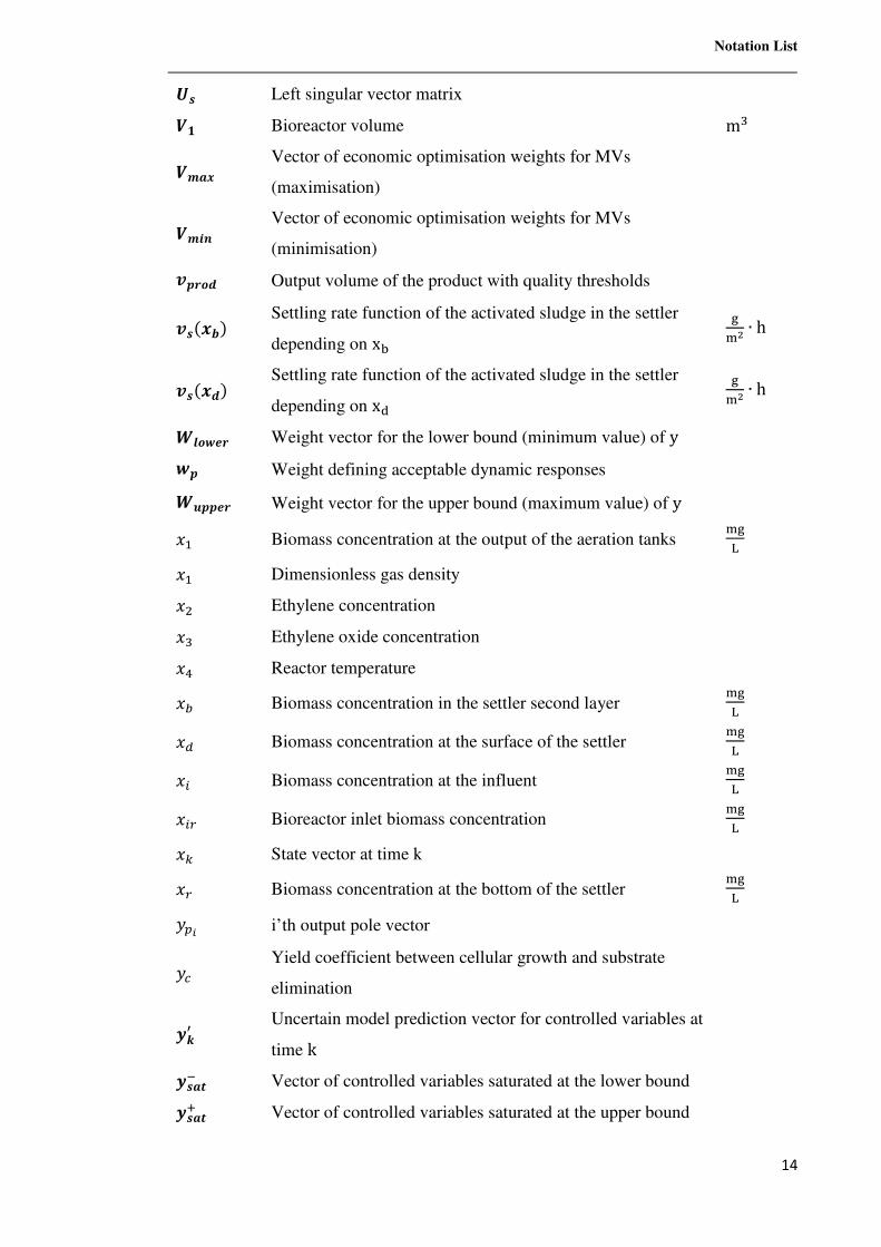
14
gi Left singular vector matrix
j� Bioreactor volume mW
j�� Vector of economic optimisation weights for MVs
(maximisation)
j�Vh Vector of economic optimisation weights for MVs
(minimisation)
�YTd� Output volume of the product with quality thresholds
�iklm Settling rate function of the activated sludge in the settler
depending on xo
��p ∙ h
�ik�m Settling rate function of the activated sludge in the settler
depending on xr
��p ∙ h
s�de�T Weight vector for the lower bound (minimum value) of y
eY Weight defining acceptable dynamic responses
s�YY�T Weight vector for the upper bound (maximum value) of y
u� Biomass concentration at the output of the aeration tanks ���
u� Dimensionless gas density
u� Ethylene concentration
uW Ethylene oxide concentration
uv Reactor temperature
uG Biomass concentration in the settler second layer ���
u, Biomass concentration at the surface of the settler ���
u' Biomass concentration at the influent ���
u'H Bioreactor inlet biomass concentration ���
u( State vector at time k
uH Biomass concentration at the bottom of the settler ���
wNx i’th output pole vector
wC Yield coefficient between cellular growth and substrate
elimination
�\y Uncertain model prediction vector for controlled variables at
time k
�i�{. Vector of controlled variables saturated at the lower bound �i�{| Vector of controlled variables saturated at the upper bound
Notation List
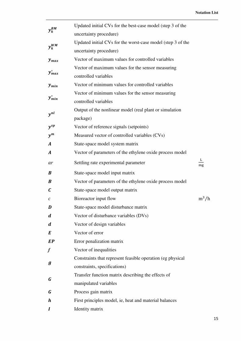
15
�\� Updated initial CVs for the best-case model (step 3 of the
uncertainty procedure)
�\s Updated initial CVs for the worst-case model (step 3 of the
uncertainty procedure)
��� Vector of maximum values for controlled variables
���∗ Vector of maximum values for the sensor measuring
controlled variables
��Vh Vector of minimum values for controlled variables
��Vh∗ Vector of minimum values for the sensor measuring
controlled variables
�h� Output of the nonlinear model (real plant or simulation
package)
�iY Vector of reference signals (setpoints)
�� Measured vector of controlled variables (CVs)
� State-space model system matrix
� Vector of parameters of the ethylene oxide process model
~� Settling rate experimental parameter ���
� State-space model input matrix
� Vector of parameters of the ethylene oxide process model
� State-space model output matrix
� Bioreactor input flow mW h⁄
State-space model disturbance matrix
� Vector of disturbance variables (DVs)
� Vector of design variables
c Vector of error
cR Error penalization matrix
f Vector of inequalities
0 Constraints that represent feasible operation (eg physical
constraints, specifications)
/ Transfer function matrix describing the effects of
manipulated variables
/ Process gain matrix
� First principles model, ie, heat and material balances
� Identity matrix
Notation List
16
� Current time discrete time
K One-degree-of-freedom proportional controller
� Number of time increments of the control horizon
n Measurement noise
M� Settling rate experimental parameter
��� Oxygen uptake rate ��� ∙ h
� prediction horizon
P Plant
P Positive definite solution of the Riccati equation
� Bioreactor input flow
U LQR weight
Z Input suppression factor
i Laplace variable
S Sensitivity Function
t Time s or h
T Complementary Sensitivity Function
� Absolute value of the vector of manipulated variables (MVs)
V Right singular vector matrix
V A locally positive function
� Yield of ethylene oxide
� Vector of controlled variables (CVs)
Notation List
17
Greek Alphabet
Symbol Definition Unit
� Auxiliary variable that denoting time
��,�. Minimum negative relative model mismatch relative to DVs
��,�| Maximum positive relative model mismatch relative to DVs
��,�. Minimum negative relative model mismatch relative to MVs
��,�| Maximum positive relative model mismatch relative to MVs
��. DV negative uncertainty matrix
��| DV positive uncertainty matrix
��. MV negative uncertainty matrix
��| MV positive uncertainty matrix
� Vector of parameters of the ethylene oxide process model
�Qx,� Realisation of the uncertainty between y� and d�
�QxP� Realisation of the uncertainty between y� and u�
���\ Matrix generated by the product between the DVs set its bounded
uncertainty realisation
���\ Matrix generated by the product between the MVs set its bounded
uncertainty realisation
� State of the ASP model
∆ Sampling period
∆�y Interval of disturbance magnitude of the uncertain model
∆�\ DV vector at k
∆�! Matrix of DV values along the prediction horizon as planned at k
∆R���� Added value, ie, product price difference between premium priced
and regular product
∆� MV movement, control action
∆�y Interval of control action magnitude of the uncertain model
∆�\ MV vector at k
∆�! Matrix of MV values along the control horizon as planned at k
∆wQx,Px?�N
Norm of the amplitude of the dynamic response of the multi-linear
system to a step at the end of the prediction horizon, for a certain
CV/MV couple
Notation List
18
∆w�# steady-state response amplitude of plant data relative to the nth
step
∆��y Prediction mismatch between the nominal model and the best-case
model
∆w',y
Change in the steady-state output prediction caused by a bounded
realisation of DV uncertainty
∆w'P Output change caused by an MV movement ∆u�
∆w',y
Change in the steady-state output prediction caused by a bounded
realisation of DV uncertainty
∆w'Py Change in the steady-state output prediction caused by a bounded
realisation of MV uncertainty
∆�Y� Model mismatch value at the end of the prediction horizon
∆������ Difference between the key CV quality threshold value for which
the price variation occurs, y�����, and the average value of the key
CV through the prediction horizon, y����
∆�sy Prediction mismatch between the nominal model and the worst-
case model
�[|
Expected deviations of uncertain parameters in the positive
direction
�[.
Expected deviations of uncertain parameters in the negative
direction
$ Weight of sub-model ϑ in the main prediction
[ Uncertain parameters
[` Lower bound on uncertain parameters
[¡ Nominal value of the uncertain parameters
[g Upper bound uncertain parameters
� Auxiliary binary variable
¢ Vector of eigenvalues
£ Relative gain array
¤ Auxiliary binary variable
¤�� Maximum growth rate of the microorganisms h.�
�YTd� Volume produced of product with quality threshold
¥ Set of possible plants
¦� Singular value

Notation List
19
¦ Vector of singular values
§ Diagonal matrix of singular values
¨ Time
©� Distance coefficient of model ϑ
ª Range of uncertain parameters
«h� Relative prediction error of sub-model ϑ relative to the nth step
«�V,���
Model mismatch between the simultaneous multi-linear prediction
system and sub-model ϑ concerning d� and y¬
«�V,�V�
Model mismatch between the simultaneous multi-linear prediction
system and sub-model ϑ concerning u� and y¬
Flexibility function
® Feasibility function
¯ Frequency
Acronyms List
20
Acronyms List
Acronym Definition
BIBO Bounded-Input Bounded-Output
BWA Analytical Bounds Worst-case Approach
CLF Control Lyapunov Function
CV Controlled variable
DAE Differential Equations
DC Disturbance Cost
DCN Disturbance Condition Number
DIC Decentralized Integral Controllable
DMC Dynamic Matrix Control
DOI Dynamic Operability Index
EMOP Economic MPC Optimisation index
EMPC Economic MPC
GDP Generalised Disjunctive Programming
GPC Generalized Predictive Control
HEN Heat Exchanger Network
HWA Hybrid Worst-Case Approach
IC Integral Controllable
ICI Controllable with Integrity
ICPS Integrated control and process synthesis
IHMPC Infinite Horizon Model predictive control
IMC Internal Model Control
IPDCF Integrated process design and control framework
ISE Integrated Squared Error
KKT Karush-Kuhn-Tucker
LCA Life Cycle Assessment
LDMC Linear Dynamic Matrix Control
LQR Linear–Quadratic Regulator
MAC Model Algorithmic Control
MIC Morari Indexes of Integral Controllability
MIDO Mixed-Integer Dynamic Optimisation
Acronyms List
21
MIMO Multiple Inputs Multiple Outputs
MINLP Mixed-Integer Nonlinear Problem
MIOCP Mixed-Integer Optimal Control Problem
MPC Model predictive control
MV Manipulated variables
NLP Nonlinear Optimisation Problem
NMPC Nonlinear Model Predictive Control
OCI Output Controllability Index
OP Operating point
OPEX Operating expenses
PID Proportional–integral–derivative
PWA PieceWise Affine
PWARX PieceWise Autoregressive Exogenous
QDMC Quadratic Dynamic Matrix Control
QP Quadratic program
RHPT Right Half-Plane Transmission
RTO Real-Time Optimisation
SARX Switched Autoregressive Exogenous
SISO Single-Input Single-Output
SMLP Simultaneous Multi-Linear Prediction
SP Setpoint
SQP Sequential Quadratic Programming
SVA Structured Singular Value Analysis
List of Figures
22
List of Figures
Fig. 1 – The typical hierarchy of control systems. ...................................................................... 32
Fig. 2 – MPC can be used to minimise the quality giveaway. .................................................... 33
Fig. 3 – Searching for the best path to the optimal operating point for a control zone system with
two controlled variables. ............................................................................................................. 35
Fig. 4 – Feedback system with controller /°, disturbance /� and plant /................................ 45
Fig. 5 – Regions of feasible operation for feasible and infeasible design (flexibility test
problem). ..................................................................................................................................... 49
Fig. 6 – How an MPC controller handles the zone control problem. .......................................... 86
Fig. 7 – Error calculation for Zone Constrained MPC. ............................................................... 86
Fig. 8 – Interfaces of an industrial MPC implementation. .......................................................... 87
Fig. 9 – The operating point moves through the boundaries of a PWA system. ....................... 100
Fig. 10 – Workflow of the joint use of the EMOP index and the SMLP. ................................. 104
Fig. 11 – EMOP index increase due to first-order soft-landing matrix for a system with 9 CVs
and unitary first-order derivative at the end of prediction. ....................................................... 127
Fig. 12 – The output prediction can be generated by multiple simultaneous states, each one with
its own update rule (SMLP system), or by a single state which continuously changes update rule
(PWA system). .......................................................................................................................... 133
Fig. 8 – The vectors connecting the operating point (±R) and �R� and �R . ......................... 136
Fig. 9 – The “degradation functions”, 0� and 0 , are functions of the “distance coefficients” ©�
and © . ...................................................................................................................................... 138
Fig. 10 – Data workflow of the first SMLP method. The distance coefficients are functions of
the output, and the new prediction is provided by the multiplication of the sub-model outputs
and the averaged weights. ......................................................................................................... 140
Fig. 11 – Data workflow of the second SMLP method. The distance coefficients are now
functions of the input vector instead of the output vector. ........................................................ 143
Fig. 12 – Data workflow of the third SMLP method. The averaged weights are now used to
obtain the new sub-states. ......................................................................................................... 146
Fig. 18 – Uncertainty in the magnitude of the steady-state output change, given a certain input
change. ...................................................................................................................................... 151
Fig. 19 – Model mismatch between sub-models 1, 2 and 3. ..................................................... 152
Fig. 20 – Uncertainty in the magnitude of an unknown input change, given a certain output
change. ...................................................................................................................................... 155
Fig. 21 – The inclusion of an anti-saturation parameter in Step 2 of the EMOP index evaluation
for uncertain models. ................................................................................................................ 160
Fig. 22 – Representation of model error for a step test. ............................................................ 161
Fig. 23 – Plant 1 – Simplified Process Flowsheet. .................................................................... 164
Fig. 24 – Plant 2 – Simplified Process Flowsheet – Plant with Product Tanks. ....................... 166
Fig. 25 – Plant 4 – Simplified Process Flowsheet – Plant with Pre-flash Drum. ...................... 167
Fig. 26 – Effect of Soft-Landing matrices _`� − 1_` − 1 for plant 1, scenario 1, for various
values of �. ................................................................................................................................ 180
Fig. 27 – Plant and controller layout for the ASP for substrate elimination. ............................ 187
Fig. 28 – Economic MPC Optimisation index versus global index defined in Eq. 181............ 197

List of Figures
23
Fig. 29 – Dynamic Response Plant A – Controlled Variables. ................................................. 198
Fig. 30 – Dynamic Response Plant A – Manipulated Variables and Disturbances. ................. 199
Fig. 31 – Predictions generated by the SMLP and PWA systems and by the ASP nonlinear
model. ....................................................................................................................................... 204
List of Tables
24
List of Tables
Table 1 – Alternative robust MPC schemes. ............................................................................... 82
Table 2 – Paper comparison of integrated process design and MPC methodologies. ................ 95
Table 3 – Crude Oil Costs and Product Prices. ......................................................................... 164
Table 4 – Description and limits for the controlled variables. .................................................. 165
Table 5 – Description and limits for the manipulated variables. ............................................. 165
Table 6 – Column Sizing Parameters for Plants 1, 2, 3 and 4. .................................................. 167
Table 7 – Energy consumption by the fired heater. .................................................................. 169
Table 8 – Increase in energy consumption by the fired heater. ................................................ 169
Table 9 – Input-based IPs identification points 1, 2 and 3. ....................................................... 173
Table 10 – Output-based IPs Identification points 1, 2 and 3. .................................................. 173
Table 11 – Residual from regression analysis for the SMLP problem. .................................... 174
Table 12 – Initial values for process outputs. ........................................................................... 175
Table 13 – Initial values for process inputs. ............................................................................. 176
Table 14 – Inputs for the scenario 1. ......................................................................................... 176
Table 15 – Output predictions for the scenario 1. ..................................................................... 176
Table 16 – Cost function values for each plant – scenario 1. ................................................... 177
Table 17 – New Crude Oil Costs and Product Prices. .............................................................. 178
Table 18 – Inputs for the scenario 1. ......................................................................................... 178
Table 19 – Output predictions for the scenario 2. ..................................................................... 178
Table 20 – Cost function values for each plant – scenario 1. ................................................... 178
Table 21 – Average index for each plant. ................................................................................ 179
Table 22 – Effect of SL matrices. ............................................................................................. 180
Table 23 – Plant 3 - uncertain model’s CVs. ............................................................................ 182
Table 24 – Plant 3 uncertain model’s MVs. .............................................................................. 183
Table 25 – Plant 3 uncertain model’s EMOP index. ................................................................. 183
Table 26 – Complexity comparison between study cases. ........................................................ 184
Table 27 – Operational, biological and physical parameters for the selected activated sludge
process. ..................................................................................................................................... 191
Table 28 – Candidate designs for the Active Sludge Process (Francisco et al., 2011). ............ 192
Table 29 – Global Index for the ASP candidate designs. ......................................................... 193
Table 30 – States of the ASP model. ........................................................................................ 194
Table 31 – ASP Process inputs. ................................................................................................ 194
Table 32 – ASP process disturbances. ...................................................................................... 194
Table 33 – EMOP index for the alternative ASP flowsheets. ................................................... 197
Table 34 – Input-based IPs identification points 1, 2 and 3. ..................................................... 202
Table 35 – Plant 1 – Sub-model 1 – Transfer Function Numerator Parameters. ...................... 229
Table 36 – Plant 1 – Sub-model 1 – Transfer Function Denominator Parameters. .................. 230
Table 37 – Plant 1 – Sub-model 2 – Transfer Function Numerator Parameters. ...................... 231
Table 38 – Plant 1 – Sub-model 2 – Transfer Function Denominator Parameters. .................. 232
Table 39 – Plant 1 – Sub-model 3 – Transfer Function Numerator Parameters. ...................... 233
Table 40 – Plant 1 – Sub-model 3 – Transfer Function Denominator Parameters. .................. 234
List of Tables
25
Table 41 – Plant 2 – Sub-model 1 – Transfer Function Numerator Parameters. ...................... 235
Table 42 – Plant 2 – Sub-model 1 – Transfer Function Denominator Parameters. .................. 236
Table 43 – Plant 2 – Sub-model 2 – Transfer Function Numerator Parameters. ...................... 237
Table 44 – Plant 2 – Sub-model 2 – Transfer Function Denominator Parameters. .................. 238
Table 45 – Plant 2 – Sub-model 3 – Transfer Function Numerator Parameters. ...................... 239
Table 46 – Plant 2 – Sub-model 3 – Transfer Function Denominator Parameters. .................. 240
Table 47 – Plant 3 – Sub-model 1 – Transfer Function Numerator Parameters. ...................... 241
Table 48 – Plant 3 – Sub-model 1 – Transfer Function Denominator Parameters. .................. 242
Table 49 – Plant 3 – Sub-model 2 – Transfer Function Numerator Parameters. ...................... 243
Table 50 – Plant 3 – Sub-model 2 – Transfer Function Denominator Parameters. .................. 244
Table 51 – Plant 3 – Sub-model 3 – Transfer Function Numerator Parameters. ...................... 245
Table 52 – Plant 3 – Sub-model 3 – Transfer Function Denominator Parameters. .................. 246
Table 53 – Plant 4 – Sub-model 1 – Transfer Function Numerator Parameters. ...................... 247
Table 54 – Plant 4 – Sub-model 1 – Transfer Function Denominator Parameters. .................. 248
Table 55 – Plant 4 – Sub-model 2 – Transfer Function Numerator Parameters. ...................... 249
Table 56 – Plant 4 – Sub-model 2 – Transfer Function Denominator Parameters. .................. 250
Table 57 – Plant 4 – Sub-model 3 – Transfer Function Numerator Parameters. ...................... 251
Table 58 – Plant 4 – Sub-model 3 – Transfer Function Denominator Parameters. .................. 252
Table 59 – Crude oil distillation – Plant 1 – Positive Uncertainty Parameters for the MVs. ... 253
Table 60 – Crude oil distillation – Plant 1 – Negative Uncertainty Parameters for the MVs. .. 253
Table 61 – Crude oil distillation – Plant 1 – Positive Uncertainty Parameters for the DV. ...... 253
Table 62 – Crude oil distillation – Plant 1 – Negative Uncertainty Parameters for the DV. .... 253

1 Introduction and Motivation
26
1 Introduction and Motivation
1.1 The Integrated Process Design and Control Framework
Optimisation methodologies are applied to several areas of chemical engineering
to solve a wide range of problems. Among these, two of the most relevant are process
control and optimal process design. Both require careful consideration at the design phase
of chemical engineering projects.
The design of a new chemical plant, or process synthesis, involves projecting
process equipment and assembling them in the correct layout to meet production goals
(carry out a chemical reaction, separation process, etc.). During the design phase, the
project engineer should optimise the correlation between return on capital and invested
capital. Sometimes achieving higher efficiency and smaller operational costs may offset
a larger initial investment, and such trade-offs are fundamental to the process synthesis
problem.
On the other hand, the design of a control system involves analysing the dynamic
behaviour of a certain plant and selecting a convenient control structure and a set of tuning
parameters to achieve the desired performance. The control system must be able to reject
disturbances successfully, and to keep stable the key variables. The unstable operation
could lead to safety and environmental constraint violations and reduced profits. Different
control structures need to be tested for any given process flowsheet, and their performance
must be evaluated and benchmarked to provide input to the decision process.
The traditional approach has been solving these problems separately, in a
sequential approach. In industrial projects, they are often carried out by different groups
of professionals with different expertise. Usually, the first step is the creation of a
flowsheet by the process design team to meet production requirements, in which the
process route, equipment layout, products and raw materials are defined based on an
optimal set of steady-state conditions. Next, the control design team evaluates process
dynamics in order to assess whether or not the desired set of operating conditions can be
achieved and maintained. The strictly necessary modifications to this end are then
proposed, i.e., at this phase changes are normally kept at the bare minimum with a view

1 Introduction and Motivation
27
to avoiding delays and friction between the teams. This situation is far from ideal because
even if control and optimal process design may often be regarded as separated areas in
chemical engineering practice, in reality, they are deeply related. Process design decisions
have a very significant impact on control system performance, which in turn is extremely
important to guarantee stable and profitable operation.
In the chemical industry, the goal of any chemical plant is to produce products
that fulfil all specifications while obtaining maximum revenue with minimum cost. To
reach such a goal it is necessary to provide the plant with a correctly engineered control
system, which must possess a convenient set of controlled and manipulated variables,
clearly defined control objectives and convenient tuning parameters. The operation must
be stable and optimised, and the plants must be operated as flexibly as possible to adapt
satisfactorily to changes in the process such as varying product demand and
specifications, and oscillation in feed composition, flowrate, pressure and temperature. In
such a context, the application of appropriate process control strategies allows for the
successful operation of the plants improving profitability by increasing product
throughput and yield of higher valued products and by decreasing energy consumption
and pollution. They also help process automation, which reduces operational costs.
Many recent works published in control theory have focused on the development
of new algorithms, but we believe this field has matured, and larger gains may be achieved
by switching the focus back to the process itself, and especially its design phase.
Assuming that the control system is well engineered, the limitations on its ability to
control and optimise chemical plants are mostly related to the plant’s characteristics.
Ultimately, the degree to which controlled variables can keep at their desired values in
the face of disturbances and saturation of control elements is defined by process
dynamics, which, in turn, is reflected in the plant’s model.
For example, plant equipment can be undersized from a control performance
perspective leading to intrinsically poor control performance. Or an exceedingly small
feed drum may imply in the impossibility of properly controlling the feed flow rate. To
avoid uncontrollable plants, a common solution has been enlarging equipment to ensure
a stable dynamic behaviour. Adding these overdesign factors certainly improves control
response, but if these are exaggerated, they may also lead to the specification of
unnecessarily expensive designs. In brief, a trade-off normally exists between capital cost
savings and the robustness of the plant design.

1 Introduction and Motivation
28
How can the correct equipment size be known? How to select the best plant
layout? The integrated process design and control framework (IPDCF) has been
suggested as an attractive alternative to overcome the issues associated with the sequential
approach traditionally used in the design of industrial process units (Sharifzadeh, 2013).
It consists of solving, iteratively or simultaneously, both the control and flowsheet design
optimisation problems while adding stability concerns as restrictions. In this way, a
systematic analysis of plant dynamics is incorporated into the process design procedure
to obtain a compromise solution between profitability and smooth and stable operation.
Significant progress has been made in the IPDCF, but untapped opportunities for
contributions remain. The present work is an addition to the IPDCF aiming at providing
a new analytical tool to assess plant design. The goal of this project is to address the
limitations possessed by currently available methodologies in some situations that will be
discussed in the next Sections.
1.2 A Classification for Integrated Process Design and Control Methods
The IPDCF is based on the fact that the achievable dynamic performance is a
property of the plant and inherent to process design. The performance will depend on
aspects of the plant units and their configuration, creating both unit and system holdups
and sensitivities, and on the type of control exercised (Morari, 1983a,b; Edgar, 2004).
The integrated design philosophy contemplates the important trade-off between
profitability and controllability, incorporating the assessment of dynamic behaviour in
the initial steps of process design. Predicting whether dynamic behaviour requirements
are met as early as possible in the design phase is greatly advantageous since this
information unlocks economic benefits and improved plant operation. Consequently,
there has been a growing recognition of the need to consider the controllability and
resiliency of a chemical process during design stage (Pistikopoulos and Van Schijndel,
1999).
According to Lewin (1999), IPDCF methods can be classified into two main
classes: (i) methods which enable screening alternative designs for controllability,
henceforth referred as Controllability Analysis; and (ii) methods which integrate the
design of the process and the control system, henceforth referred as Integrated Control
and Process Synthesis (ICPS). The fundamentals of both classes are now going to be
provided, but further details can be found in the Literature Review, Chapter 2.
1 Introduction and Motivation
29
The first class focuses on plant controllability. Roughly, the concept of
controllability denotes the ability to control the main variables of a process unit around
their desirable values using only certain admissible manipulations. The exact definition
varies within the framework or the type of models applied. Controllability is a concept
that arises from the analysis of the fundamental limitations to the performance of control
systems, which were first studied in a systematic way in Morari (1983a,b) making use of
the perfect control concept. These studies gave birth to a series of indicators for the
evaluation of open and closed-loop controllability, allowing comparison and
classification of flowsheets regarding operational characteristics. Some measures using
this concept include resiliency indices (Morari, 1983b), disturbance condition numbers
(Skogestad and Morari, 1987) and the relative disturbance array (Stanley, Marino-
Galarraga and McAvoy, 1985).
While this class of methods has the advantage of being easily integrated into
traditional design procedures, the indices are often calculated based on either steady state
or linear dynamic models, introducing significant approximations and reducing the rigour
of the analysis. Also, the relation between the indices and the closed-loop performance
may be unclear, which becomes evident by the large number of papers where the authors
verify their findings through closed-loop dynamic simulations (Lewin, 1999).
Controllability Analysis received a large number of contributions in the decades of 1980s
and 1990s, but fewer in recent years. Formal definitions of the measures and methods of
Controllability Analysis are given in Sections 2.1.1 and 2.1.2.
The second class, ICPS, consists of solving mass and energy balances for the
flowsheet, sizing equipment and evaluating control performance at the same time for a
certain flowsheet. The simultaneous optimisation of both the process and the control
scheme is parameterised by means of a so-called superstructure in which dynamic
performance requirements are included as constraints to optimal design. The aim is
replacing the methods for early process synthesis traditionally used to obtain flowsheets,
which rely on heuristic methods and simulation, by a single layer optimisation problem
with embedded control structures. Alternative designs can be compared based on, for
example, the Integrated Squared Error (ISE) for specific disturbance scenarios
(Schweiger and Floudas, 1999), evaluating the system's dynamic feasibility and stability.
Methods of this class can be numerically intensive, limiting their applicability to
small or medium scale case studies and requiring specific assumptions on the control
1 Introduction and Motivation
30
system to be used. However, aided by the ever-increasing availability of computing
power, the ICPS has received several contributions in recent years, and there is already a
sizable body of work continuously expanding its practical applicability. In most of these
works, a correlation between key sizing/layout parameters and control performance is
established resulting in a cost function for which an optimisation solver will attempt to
find the global solution. Structural changes in the process design and the control structure
can be incorporated by adding integer decisions in the analysis by solving an intensive
MINLP (Mixed Integer Nonlinear Programming) formulation. However, the addition of
integer variables increases the problem's dimensionality, turning it even more expensive
regarding required computing power and time. A downside to ICPS is that, if the
optimisation is too radical, flowsheets thus designed may depend on the good functioning
of the control system to be stable. Problems with sensors and control elements such as
valves are bigger issues for these precisely designed plants which, by design, have little
room available for control system malfunctioning. ICPS is discussed in further detail in
Chapter 2 for classic feedback control, and in Section 2.3 for Model Predictive Control.
1.3 Model Predictive Control and the Monetisation of Control
Performance
One way of monetising control performance is to evaluate the profitability or
OPEX (Operating expenses) of the industrial unit with the control system activated, then
deactivate the system and evaluate it again, and then subtract the latter figure from the
former. The difference observed, i.e, the increase in profit (or reduction of expenses), can
be explained by the reduced variability of the operating conditions that arise from the
actions of the control system when the system successfully controlled.
But how does reduced variability leads to higher revenue? It allows the operating
team to drive the process closer to restrictions, enabling the reduction of the product
quality giveaway. The giveaway gap is the difference between the quality of the product
and the quality specification. It means that the manufacturer produces products of better
quality than needed, which has an effect on the cost (lower yield, more energy, higher
temperature, more reflux, etc.). Restrictions related to safety also restrict profitability,
e.g., the maximum temperature and pressure admissible by a chemical reactor nay restrict
conversion. Hence a well-engineered control system is able to maximise operating
revenue of the plant through the expansion of the range of feasible and stable operating
points (OP), which can be sustained without producing off-spec products or
compromising safety.
1 Introduction and Motivation
31
Any configuration of the control system is able defines the sustainable OP range
up to a certain degree, but some types of controllers yield broader ranges than others and
for the same control system configuration, the tuning parameters being used also affect
the OP range. Most of the methodologies developed for the IPDCF of chemical processes
have feedback controllers such as PID (proportional–integral–derivative) embedded in
the analysis. PIDs are SISO (Single-Input Single-Output) feedback controllers, which
normally operate with a single setpoint (SP), and are standard in the chemical industry as
well as numerous other applications. Ideally, SPs are set at each variable’s economic
optimal OP, as defined by the project team.
In practice, for multivariable problems, this approach introduces a well-known
conflict between control goals. The issue arises as each PID tries to keep its controlled
variable (CV) at the required SP without regard to disturbing other variables. Since most
systems do not possess enough degrees of freedom, either due to the lack of manipulated
variables (MV) or saturation of control elements, meeting all control goals simultaneously
is frequently impossible (González and Odloak, 2009). Advanced “decoupling”
techniques can help lessen the problem, but nevertheless, interactions between controllers
inevitably impose limits to feasible OPs. In short, one should look at the bigger picture
and consider the problem of interactions between SISO controllers to define optimal SPs.
Model Predictive Control (MPC) is a more powerful kind of control structure that
has matured for almost four decades of development in which it has been widely
implemented and recognised. MPC control schemes are popular solutions to meet the
control requirements of complex chemical processes due to their capacity for handling
multivariable systems with the inverse response, as well as time delayed and highly
nonlinear systems. MPC is a far more suitable for use with MIMO (Multiple Inputs
Multiple Outputs) systems with strong interactions since it controls simultaneously all
variables and minimises the global error according to control goal prioritisation (Morari
and Lee, 1999). More information concerning MPC is provided in Section 2.2.
The MPC packages may replace PID controllers entirely in some processes, but
they are more commonly encountered operating in conjunction with them. In this
arrangement, MPCs normally occupy a higher position in the control hierarchy and
provide SPs to PIDs (Scattolini, 2009). Moreover, by introducing economic goals in their
objective functions or integrating with a Real-Time Optimisation (RTO) layer, some
MPC schemes are designed to drive the plant as close as possible to the economically
optimal operating point (Limon et al., 2013). Fig. 1 presents the standard hierarchy of
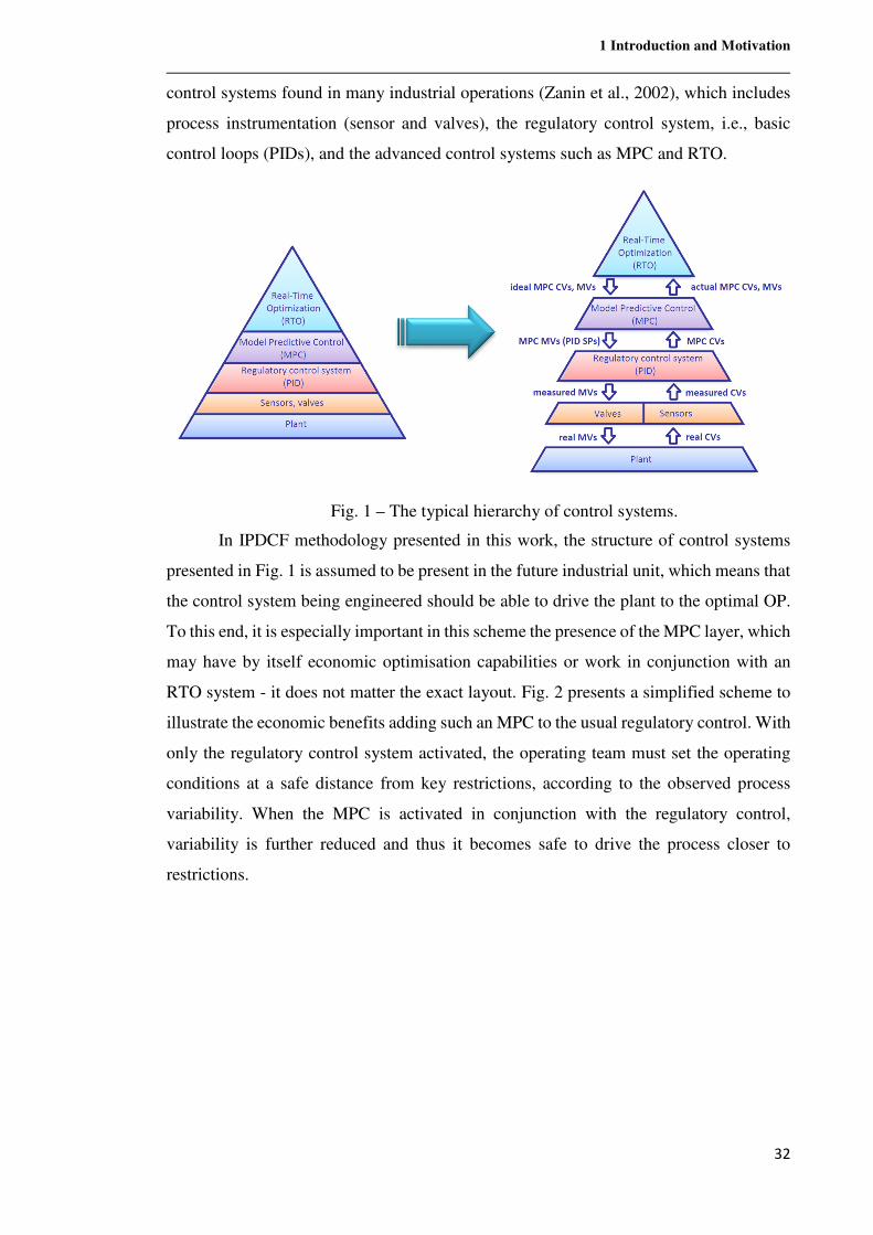
1 Introduction and Motivation
32
control systems found in many industrial operations (Zanin et al., 2002), which includes
process instrumentation (sensor and valves), the regulatory control system, i.e., basic
control loops (PIDs), and the advanced control systems such as MPC and RTO.
Fig. 1 – The typical hierarchy of control systems.
In IPDCF methodology presented in this work, the structure of control systems
presented in Fig. 1 is assumed to be present in the future industrial unit, which means that
the control system being engineered should be able to drive the plant to the optimal OP.
To this end, it is especially important in this scheme the presence of the MPC layer, which
may have by itself economic optimisation capabilities or work in conjunction with an
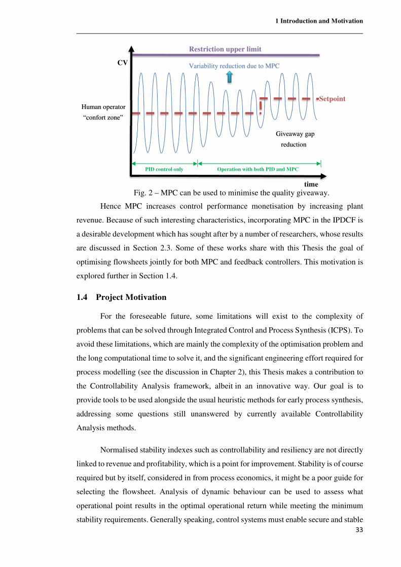
RTO system - it does not matter the exact layout. Fig. 2 presents a simplified scheme to
illustrate the economic benefits adding such an MPC to the usual regulatory control. With
only the regulatory control system activated, the operating team must set the operating
conditions at a safe distance from key restrictions, according to the observed process
variability. When the MPC is activated in conjunction with the regulatory control,
variability is further reduced and thus it becomes safe to drive the process closer to
restrictions.
1 Introduction and Motivation
33
Fig. 2 – MPC can be used to minimise the quality giveaway.
Hence MPC increases control performance monetisation by increasing plant
revenue. Because of such interesting characteristics, incorporating MPC in the IPDCF is
a desirable development which has sought after by a number of researchers, whose results
are discussed in Section 2.3. Some of these works share with this Thesis the goal of
optimising flowsheets jointly for both MPC and feedback controllers. This motivation is
explored further in Section 1.4.
1.4 Project Motivation
For the foreseeable future, some limitations will exist to the complexity of
problems that can be solved through Integrated Control and Process Synthesis (ICPS). To
avoid these limitations, which are mainly the complexity of the optimisation problem and
the long computational time to solve it, and the significant engineering effort required for
process modelling (see the discussion in Chapter 2), this Thesis makes a contribution to
the Controllability Analysis framework, albeit in an innovative way. Our goal is to
provide tools to be used alongside the usual heuristic methods for early process synthesis,
addressing some questions still unanswered by currently available Controllability
Analysis methods.
Normalised stability indexes such as controllability and resiliency are not directly
linked to revenue and profitability, which is a point for improvement. Stability is of course
required but by itself, considered in from process economics, it might be a poor guide for
selecting the flowsheet. Analysis of dynamic behaviour can be used to assess what
operational point results in the optimal operational return while meeting the minimum
stability requirements. Generally speaking, control systems must enable secure and stable
Restriction upper limit
Setpoint
PID control only Operation with both PID and MPC
CV
time
Human operator
“confort zone”
Variability reduction due to MPC
Giveaway gap
reduction
1 Introduction and Motivation
34
process operation, environmental compliance, on spec product quality and economic
optimality. Since these goals are deeply related to plant revenue and can often be
translated into monetary values, monetising control performance is possible and arguably
should be one of the objectives of Controllability Analysis. For this reason, it would be
desirable to have an approach relating explicitly the process dynamics and the amount of
the control effort to operational revenue.
The speed with which a controller can return the process to the original operating
region is less important than the ability to operate close to the restrictions on the controlled
variables since it is a well-known fact that economically optimum OPs usually lie on
constraint intersections (Narraway and Perkins, 1993). Nowadays it is not such a strong
assumption that, if sensors and control elements work properly, every one of the available
world-class MPC packages will be able to drive the process to this optimal OP (Angeli,
2012) since they possess economic optimisation capabilities. But if we can assume this
as a fact, how should the design of chemical processes be affected? This Thesis provides
a new methodology with embedded MPC that can be used to select the best among a
number of candidate process designs for any given continuous or semi-continuous
process. The following questions need to be addressed to accomplish this goal:
• Within the range of all possible operating points or conditions available
for a given plant, what is the most profitable?
• Is the path from an arbitrary initial operating point to this desired point
feasible? Does it violate operational constraints? To what extent? Are
these violations acceptable?
• Can the optimal operating point be sustained by the said plant?
• Given a number of different plant designs, how does each plant’s optimal
operating point compares based on revenue?
• Given a set of controlled and manipulated variables and their bounds, what
effect has a certain plant layout modification on monetised MPC
performance?
• How changes in product specifications affect plant revenue? Should they
lead to further changes in the layout?
Hence, the problem being addressed is finding the optimal feasible operating point
that exists within the range of possible conditions for a certain flowsheet while assuming
MPC. To this end, we must also consider control goal definitions of the embedded MPC
1 Introduction and Motivation
35
structure, which affect this problem. While the optimal operating point analysis will be
similar to that of PIDs if the embedded MPC has fixed SPs, MPC can also operate with
flexible control goals known as “control zones”. The use of control zones changes how
the optimal feasible operating point of a flowsheet is defined in comparison to a fixed SP
approach. In this case, a variable can move inside its control zone without penalisation
(see the description of this MPC formulation in Section 2.2.2). Fig. 3 presents a diagram
showing that the interaction of control and process design can affect not only the optimum
operating point but also the desired trajectory to reach it from an initial state.
Fig. 3 – Searching for the best path to the optimal operating point for a control zone system with two controlled variables.
Zone constrained MPC has become the advanced control method of choice in the
chemical industries such petroleum refining and petrochemical processes. Being a very
useful variant of MPC, it is time for a methodology addressing it to be included in the
IPDCF. Hence, a method to assess dynamic behaviour valid for any zone constrained
MPC is presented in this Thesis. It consists of evaluating in a number of scenarios the
Economic MPC Optimisation (EMOP) index of each alternative plant design. The EMOP
index is an assessment tool based on a monetised measure of the required control effort,
enabling flowsheet benchmark.
1.5 Thesis Organisation
This Thesis is organised into eight Chapters. This introduction was the first
Chapter. Chapter 2 is the Literature Review, which contains a comprehensive review of
the IPDCF (Integrated Process Design and Control Framework), a short review of MPC
and a review of existing IPDCF strategies that embed MPC structures. Chapter 3 details
the EMOP index methodology, a new IPDCF method; Chapter 4 contains the

1 Introduction and Motivation
36
Simultaneous Multi-Linear Prediction (SMLP), a multiple state-space model approach
developed to improve the accuracy of the EMOP index by reducing nonlinearity-related
error. In Chapter 5, an extension is presented to address the issue of model uncertainty.
Chapter 6 features a case of study concerning the assessment of four possible layouts for
a crude oil distillation unit for which the full methodology is applied. The results obtained
for this case study are discussed and interpreted. Chapter 7 compares the EMOP index
methodology to another integrated process design and control method by applying them
to the same case study, the active sludge of a wastewater treatment plant. In Section 7.2,
the same model is used to benchmark the SMLP in comparison to other multi-model
approaches. Final conclusions are presented in Chapter 8.
2 Literature Review
37
2 Literature Review
This Literature Review Chapter of this PhD Thesis presents a comprehensive
survey of the Integrated Process and Control Design Framework.
2.1 Review of Integrated Process and Control Design Methodologies
The main contribution of this Thesis can be classified as part of the Integrated
Process and Control Design Framework, and for this reason, a general view of it is
presented in this Chapter. Relevant concepts are presented in this Chapter intending to
provide a theoretical background for the EMOP index methodology. This Literature
Review is organised in following items:
1. Concepts and Measures of Controllability;
2. Process-Oriented Methods for Controllability Analysis;
3. Integrated Process Design and Control Framework - Methods of Integrated
Control and Process Synthesis;
4. Review of Model Predictive Control;
5. Review of Integrated Process Design and Model Predictive Control
Methodologies;
6. The Linear Hybrid Systems framework;
7. Conclusions from the Literature Review.
Key controllability concepts and measures are discussed in the first item, as well
as the fundamental limitations to control performance. The second item focuses on
Controllability Analysis methods that deal with complications such as systems with
recycles, systems with steady-state multiplicity and methods that integrate rigorous
modelling and passivity theory. The third item presents methods with embedded
Controllability Analysis which also present integrated design optimisation problems.
Such integrated problems have design variables to affecting feedback control structures,
plant layout and sizing parameters. These first three items make up the bulk of the IPDCF.
Being numerous and sharing fewer similarities to the EMOP methodology, these works
are only briefly discussed, with a view to the completeness of this review, through Section
2.1.

2 Literature Review
38
The fifth item is discussed in Section 2.3 and consists of integrated design and
control papers with embedded MPC. Since there are few papers in this category and these
are more closely related to this PhD project, an elaborate discussion is provided for each
one of them. Item four consists of a quick introduction to MPC, which is presented in
Section 2.2.
2.1.1 Concepts and Measures of Controllability
This Section introduces a series of efforts made over the years towards measuring
controllability. A plant is controllable if there exists a controller (connecting plant
measurements and plant inputs) that yields acceptable performance for all expected plant
variations (Skogestad and Postlethwaite, 1996). According to this view, controllability is
independent of the controller, being a property of the plant (or process) alone. Thus, it
can only be modified by changing the plant itself, that is, by (plant) design changes. Such
changes may include:
• Changing the apparatus itself, e.g. type, size, layout, etc.;
• Relocating sensors and actuators;
• Adding new equipment to dampen disturbances;
• Adding extra sensors;
• Signal Processing, e.g., signal filter;
• Adding extra actuators;
• Changing the control objectives.
A plethora of methods were proposed over the years with the purpose of
evaluating a plant’s sensitivity to disturbances, which can be controller-independent
(open loop analysis) or not (closed loop analysis). ‘Controllability Analysis’ currently
covers to the assessment of flowsheet properties such as State Controllability, resiliency,
flexibility, operability, switchability and stability, among others, all of which will be
reviewed in the next subsections. These measures are often summarised in the form of
indexes that show the effects of perturbations on controlled variables and operational
constraints and their propagation through the process.
Let us start this discussion on methods of Controllability Analysis defining the
“Input-Output” controllability. The evaluation of controllability was first introduced by
Ziegler and Nichols (1943). Skogestad and Postlethwaite (1996) provided the following
definition for Input-Output controllability:
2 Literature Review
39
Definition 2.1.1.1 Input-output controllability is the ability to achieve
acceptable control performance; that is, to keep the outputs (�) within
specified bounds or displacements from their references (�iY), in spite of
unknown but bounded variations, such as disturbances (�) and plant
changes (including uncertainty), using available inputs (�) and available
measurements (�� or ��).
This seminal idea implies that the process performance depends on the
availability of both measured and manipulated variables. Input-Output Controllability can
also be described as the ability of an external input (the vector of controlled variables) to
move the output from any initial condition to any final condition in a finite time
interval. Note that being controllable, in this narrow definition of controllability, does not
mean that once a state is reached, that state can be maintained. It merely means that said
state can be reached within a reasonable timeframe. Later methodologies for investigating
the open-loop, input-output controllability of a process include Biss and Perkins (1993).
The concept of “input-output” controllability, insufficient as it is to guarantee
proper closed-loop dynamic behaviour, paved the way to a broader theoretical
background and more restricted definitions. For instance, Integral controllability is
another, more rigorous, criterium. According to Campo and Morari (1994), a plant with
a given control configuration is Integral Controllable (IC) if it is stable with all controllers
operating and suitably tuned and remains stable when the gains of all controllers are
detuned simultaneously by the same factor ∈ µ0,1·. If multiloop SISO controllers are
used, integral controllability is an important criterion in the variable pairing. Yu and
Luyben (1986) eliminated pairings with negative Morari Indexes of Integral
Controllability (MIC) to ensure integral controllability. The MICs are the eigenvalues of
the G|k0m matrix (the plant steady-state gain matrix with the signs adjusted so that all
diagonal elements have positive signs). If all of the individual loops are integrally
controllable, a negative value of any of the eigenvalues of G|k0m means that the variable
pairing will produce an unstable closed-loop system if each loop is detuned at an arbitrary
rate. It should be noticed that for 3 x 3 or higher order systems, there are instances for
which no variable pairing will give MICs that are all positive.
Campo and Morari (1994) also defined systems which are Controllable with
Integrity (ICI), i.e., a system that is IC, and remains IC, if any number and combination
of controllers are taken out of service (set on manual mode).
2 Literature Review
40
Even if more restrictive, ICI is not yet the ideal degree of controllability. Usually,
it is desired to design systems that reach the classification of Decentralized Integral
Controllable (DIC). The system is DIC if it is ICI and remains stable when any number
of controllers are detuned by individual factors ' ∈ µ0,1·, ¹ = 1,… , MC, where MC is the
number of active controllers. Besides being the most demanding property, DIC is also the
one most difficult to ascertain because of the complexity of the problem (Skogestad and
Morari, 1988).
Also, Wolff et al. (1992), Wolff et al. (1994) and Wolff (1994) propose procedures
to evaluate the inherent control properties of chemical plants using analytic tools. Wolff
et al. (1992) present a method to assess linear controllability, combining different
controllability measures (RGA, Section 2.1.1.7, DCN, 2.1.1.6, among others) that
complement each other for an enhanced understanding of the process behaviour. In Wolff
et al. (1994) a systematic study of the operability and decentralised control system design
of the total plant is presented. It involves the optimised selection of manipulated and
controlled variables, and flexibility and Controllability Analysis using linear
controllability indices.
The Controllability Analysis based on dynamic models may be carried out by
computing some indicator of the evolution of model outputs throughout a predefined time
horizon. A typical technique is to obtain the integral of the square control error (ISE)
using the dynamic nonlinear model. Some examples of the use of this index can be found
in Schweiger and Floudas (1997), Bansal et al. (1998), Asteasuain et al. (2006, 2007) and
Revollar et al. (2010a). Also in Flores-Tlacuahuac and Biegler (2007), where aside from
the ISE, they use additionally the time to steady state. In Exler et al. (2008) a set of
performance indexes, including the ISE and other open loop measures, is evaluated for
the activated sludge process, as well as pumping energy and the aeration energy in the
system (the same process used as case study in Chapter 7).
2.1.1.1 State Controllability
Over the years the rise of the state-space framework enabled further controllability
definitions. The state of a deterministic system is the set of values of all the system's state
variables (those variables characterised by dynamic equations), that completely describes
the system at any given time. In particular, if the states at present and all current and future
values of the control actions are known, no additional information on the system is needed
to predict future conditions.
2 Literature Review
41
The term ‘State Controllability’, is a concept first introduced by Kalman (1960)
that describes the ability of an external input to move the internal state of a system from
an initial state to any other final state in a finite time interval. A system is state-
controllable if there exists an input which can achieve the desired state in a given time
(Ogata, 1997). Skogestad and Postlethwaite (1996) provided a formal definition for State
Controllability:
Definition 2.1.1.1.1 State Controllability. The dynamical system ¼ =� + ��, or equivalently the pair k�,�m, is said to be state controllable if,
for any initial state k¾m = ¾, any time ¿� > 0 and any final state �, there
exists an input �k{m such that k{�m = �. Otherwise the system is said to be
state uncontrollable.
Rosenbrock (1970) gives a thorough discussion of the issues of State
Controllability and also defines the term ‘functional controllability’, defined as the
capability of a dynamical system of having its output changed to reproduce certain
trajectories belonging to given a class output sub-spaces. This concept turns out to be
related to the property of ‘invertibility’ of the process model, as investigated in Morari
(1983a,b). Additionally, some particular concepts of controllability and observability for
nonlinear systems in state-space are developed in Hermann and Krener (1977). A system
is State Observable if we can obtain the value of all individual states by measuring the
output wk¿m over some time period. According to Skogestad and Postlethwaite (1996),
State Observability can be defined as follows:
Definition 2.1.1.1.2 State Observability. The dynamical system ¼ =� + ��, � = � (or the pair k�, �m) is said to be State Observable if,
for any time ¿� > 0, the initial state k¾m = ¾ can be determined from
the time history of the input �k{m and the output�k{m in the interval µ0;¿�·. Otherwise the system, or k�, �m, is said to be state unobservable. Let Â' be
the i’th eigenvalue of �, ¿' be the corresponding eigenvector, �¿' = �Â', and wNx = �¿' the i’th output pole vector. Then the system k�, �m is State
Observable if and only if wNx ≠ 0, ∀¹.
In words, a system is State Observable if and only if all its output pole vectors are
nonzero. Some works are found in the literature where the methodology to integrate
design and control focuses in analysing the State Controllability of nonlinear systems.
The works by Ochoa (2005) and Ochoa and Alvarez (2005), are interesting contributions

2 Literature Review
42
where the integrated design is carried out to ensure the local controllability of input affine,
nonlinear systems, by means of some metrics for practical controllability based on state-
space theory. They concern different aspects of the process, such as the available degrees
of freedom for control, the rank of the local controllability matrix, the system invertibility,
and the range of available control actions and the existence of a linear reachability
trajectory. These indices are examined to address problems such as misleading
interactions between inputs and states, wrong selection of manipulated variables or final
control elements and physical restrictions of the states, which preclude the assurance of
practical controllability. The procedure uses the phenomenological model of the process
and selects the manipulated variables and the best structure (pairing) for control. It also
includes the determination of the available operation range for the input variables and the
selection of perturbations tolerances under different scenarios. The method addresses the
plant optimisation as a function of the investment and operation costs while including the
evaluation of the controllability metrics and considering the restrictions imposed by them.
At last, the control system is designed to suit the optimal plant, knowing that its
controllability is assured at the desired operating point. Authors present an ammonium-
water separation process with a reactor-flash-exchanger plant, as a design example.
An extension of this work to undertake the integrated design of coupled systems
is found in Munoz et al. (2008), where a methodology is proposed to verify the
controllability of coupled systems based on the computation of the accessibility
distribution and the controllable/non-controllable states decomposition. In Alvarez
(2008) the Hankel Matrix is proposed as controllability measure. In Lamanna et al. (2009)
the state-space practical Controllability Analysis is used to impose restrictions in the
integrated design of a sulfidation tower by integrated-optimisation methods. Calderón et
al. (2012a) propose the redesign for a wastewater treatment plant based on the results of
the nonlinear State Controllability Analysis of the system. The set theory is used to check
the controllability limits of the system including disturbances limits and constraints on
control inputs. In Calderón et al. (2012b) a comparison between differential geometric
and set-theoretical (randomised algorithms) methods to consider the nonlinear State
Controllability is presented. A detailed description of the methodology to assess nonlinear
State Controllability in the integrated design framework can be found in Alvarez (2012).
2.1.1.2 Dynamic Resiliency - Perfect Control and its Limitations
Morari (1983a, 1983b) suggested making the problem of controllability
assessment independent of the controller selection problem. This is done by finding a
2 Literature Review
43
plant's best achievable closed-loop control performance for all possible constant
parameter linear controllers. This target, the upper bound on the achievable closed-loop
performance, is defined as the plant's dynamic resilience. Thus, "dynamic resilience" is
an expression of the plant's inherent limitation on the closed-loop system's dynamic
response which is not biased by specific choices of controllers. Furthermore, dynamic
Resiliency is concerned with fast and smooth changeover and recovery from process
disturbance, with the ultimate goal of determining the inherent dynamic characteristic of
a plant independently of the selection of a particular controller or another.
The higher the Dynamic Resilience of a plant the closer it is to be a perfectly
controllable plant, i.e., a plant for which perfect control is achievable. Perfect control can
be defined as a series of control actions such that all the outputs are held at their nominal
values in the steady state, i.e., no offset occurs. Hence, a perfect controller ensures total
disturbance rejection. Let us consider a linear transfer function model of the form given
by Eq. 1:
�kim = /kim�kim + /�kim�kim Eq. 1
where � is the vector of manipulated variables (MVs), � is the vector of
disturbance variables (DVs), � is the vector of controlled variables (CVs) and / and /�
are transfer function matrices describing respectively the effects of MVs and DVs. All
these parameters of Eq. 1 are Laplace transforms in the s-domain, where s is a complex
number frequency parameter. The objective is to minimise the error, c = � − �iY, where
�iY is the vector of reference signals (setpoints). Perfect control is theoretically possible
when we have at least as MVs inputs as CVs. Mathematically, the set of perfect control
actions is defined as the solution to the following problem:
g�Vh = ��� �Vh�‖�‖ i. {./� + /�� = ¾ Eq. 2
Where omitted the Laplace transfer function notation. For square plants (same
number of inputs and outputs) the perfect control problem of Eq. 2 has a unique solution
given by Eq. 3:
� = −/.�/�� Eq. 3
Eq. 3 represents a perfect feedforward controller, assuming d is measurable. An
important fact is that perfect control requires the controller to somehow generate an
inverse of G. According to Morari (1983a), perfect control cannot be achieved if:
2 Literature Review
44
• / contains Right-Half-Plane-Transmission zeros (since then /.� is
unstable and has an inverse response, see Section 2.1.1.4);
• / contain time delays (since then /.� contains a prediction);
• / has more poles than zeros (since then /.� is unrealisable);
• / is uncertain (since then the exact /.� cannot be obtained);
• Input vector �kim reaches saturation.
Since one or more of those restrictions are always present for industrial plants,
perfect control is not physically realisable (Skogestad and Wolff, 1992). Controllability
Analysis involves using qualitative and quantitative methods to assess how controllable
is a plant, i.e., how close its achievable control performance is to perfect control.
Let us address the issue of model uncertainty. / may be uncertain due to a series
of factors. For instance, frequently the exact values of parameters that are inputted to the
model are unknown and cannot be exactly inferred. Another kind of uncertainty is the
parametric variability, that comes from the variability of input variables of the model.
Structural uncertainty may also be presented, which is also known as model inadequacy,
model bias, or model discrepancy. It depends on how accurately a mathematical model
describes the true system for a real-life situation, because models are almost always only
approximations to reality. Algorithmic uncertainty, also known as numerical uncertainty
or discrete uncertainty, arises from numerical errors and numerical approximations per
implementation of the computer model, whose implementation is necessary when models
are too complicated to solve exactly (a frequent situation in chemical engineering).
Experimental uncertainty, also known as observation error, this comes from the
variability of measurements, which is inevitable and can be noticed by repeating a
measurement for many times using the same settings for all inputs/variables. Details
concerning the plethora of uncertainty definitions can be found in Iman and Helton
(1988). An adequate definition of model uncertainty for the purpose of process control
was provided in Skogestad and Morari (1986):
Definition 2.1.1.2.1 Model uncertainty. Assuming that the plant R is linear
and time invariant, but that its exact mathematical description is unknown.
However, it is known to be in a specified “neighbourhood” of the “nominal”
system, whose mathematical “model” RS is available. This neighborhood
will be denoted the uncertainty “set”; it defines the set of possible plants ¥.
In some cases the uncertainty set ¥ may include a finite number of plants.
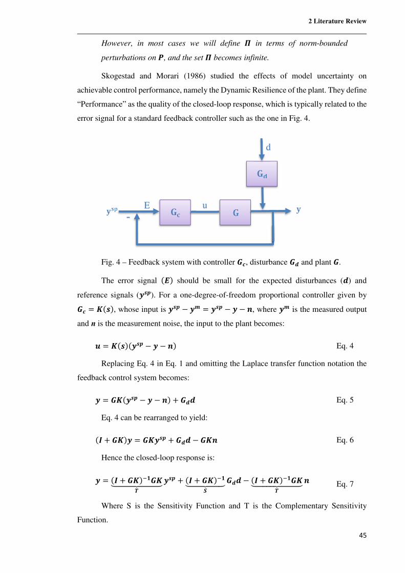
2 Literature Review
45
However, in most cases we will define ¥ in terms of norm-bounded
perturbations on R, and the set ¥ becomes infinite.
Skogestad and Morari (1986) studied the effects of model uncertainty on
achievable control performance, namely the Dynamic Resilience of the plant. They define
“Performance” as the quality of the closed-loop response, which is typically related to the
error signal for a standard feedback controller such as the one in Fig. 4.
Fig. 4 – Feedback system with controller /°, disturbance /� and plant /.
The error signal kcm should be small for the expected disturbances (�) and
reference signals (�iY). For a one-degree-of-freedom proportional controller given by
/° = !kim, whose input is �iY − �� = �iY − � − h, where �� is the measured output
and n is the measurement noise, the input to the plant becomes:
� = !kimk�iY − � − hm Eq. 4
Replacing Eq. 4 in Eq. 1 and omitting the Laplace transfer function notation the
feedback control system becomes:
� = /!k�iY − � − hm + /�� Eq. 5
Eq. 4 can be rearranged to yield:
k� + /!m� = /!�iY + /�� − /!h Eq. 6
Hence the closed-loop response is:
� = k� + /!m.�/!ÇÈÈÈÈÉÈÈÈÈÊb
�iY + k� + /!m.�ÇÈÈÉÈÈÊ_
/�� − k� + /!m.�/!ÇÈÈÈÈÉÈÈÈÈÊb
h Eq. 7
Where S is the Sensitivity Function and T is the Complementary Sensitivity
Function.
ËÌÍ ÎÏ Î Ë -
E u
ÎÐ
d
2 Literature Review
46
The control error is
c = � − �iY = −_�iY + _/�� − bh Eq. 8
In Eq. 8 we have used the fact that b − � = −_. The corresponding plant signal is
provided by
� = !_�iY −!_/�� − !_h Eq. 9
When the measurement noise can be neglected the Sensitivity Function (_)
describes the relationship between �iY, d and E. The term Sensitivity Function is natural
because S gives the sensitivity reduction afforded by feedback.
c = � − �iY = _k/�� − �iYm Eq.10
To have "good" performance, _ has to be ''small". The magnitude of S may be
measured using the singular value ¦�. At a given frequency Ó, ¦�Ô_kÕÓmÖ represents the
"worst" amplification k‖c‖� ‖/�� − �iY‖�⁄ m of k/�� − �iYm. By "worst" we mean that
k/�� − �iYm is in the direction giving rise to the largest amplification. A typical
performance specification is provided by Eq. 11:
c¦�k_m ≤ ØeYØ.�
Eq. 11
where eYkim is a weight which is used to define what dynamic responses are
acceptable. Therefore, the Sensitivity Function is a measure of the Dynamic Resilience
of a plant.
Weitz and Lewin (1996) proposed a procedure for Dynamic Resilience analysis
that relies on a modelling strategy which makes use of linear approximations, which are
obtained from the simulation of the steady-state flowsheet. Karafyllis and Kokossis
(2002) introduced Disturbance Resiliency Index (DRI) as a measure for the integration
of design and control. The measure reflects on the ability of the process to reject
disturbances and prevent saturation in the manipulated variables. The measure is defined
mathematically, and a set of properties and theorems are proved to enable its use. For a
large number of systems and networks, the application of the theory yields analytical
expressions one can study and analyse. In other cases, it yields bounding expressions that
one can embed in optimisation formulations and mathematical models. The measure
quantifies the disturbance resiliency properties of a process. Compared to the works of
Halemane and Grossmann (1983) and Grossmann, Halemane and Swaney (1983), it has
the advantage of a clear extension to the dynamical properties of the system.
2 Literature Review
47
2.1.1.3 Feasibility and Flexibility Analysis
Flexibility is the ability to obtain feasible steady-state operation at a number of
given operating points, i.e. over a range of uncertain conditions. These uncertain
conditions can be defined from expected variations in raw material and process
performance.
The flexibility analysis involves two important problems: the feasibility test and
the quantification of the inherent flexibility of a process (Grossmann and Morari, 1984).
The feasibility test problem determines the existence of at least one set of manipulated
variables that can be selected during plant operation, such that, for every possible
realisation of the uncertain parameters all the process constraints are satisfied (Halemane
and Grossmann, 1983).
Let us see how these problems we can be systematically addressed through
mathematical formulations developed by Grossmann and co-workers (Grossmann et al.,
1983; Grossmann and Straub, 1991). We will consider simple vertex solution methods as
well as an active set method, which does not necessarily have to examine all the vertex
points or even assume that critical points correspond to vertices. The basic model assumed
for the flexibility analysis involves the following vectors of variables and parameters: �,
the vector of design variables corresponding to the structure and equipment sizes of the
plant; the state variables that define the system (e.g. flows, temperatures); � the control
variables that can be adjusted during operation (e.g. flows, utility loads), [ the uncertain
parameters (e.g. inlet conditions, reaction rate constants). Eq. 12 represents a first
principles model, i.e., heat and material balances:
�k�, , �, [m = 0 Eq. 12
where by definition dimÚ�Û = dimÚÛ. The constraints that represent feasible
operation (e.g. physical constraints, specifications) are given by Eq. 13:
0k�, , �, [m ≤ 0 Eq. 13
Although in principle flexibility can be analysed directly in terms of Eq. 12 and
Eq. 13, for simplicity in this discussion the state variables from Eq. 12 are eliminated. In
this way, the state variables become an implicit function of �, � and [. That is, =k�, �, [m. Eq. 13 thus becomes:
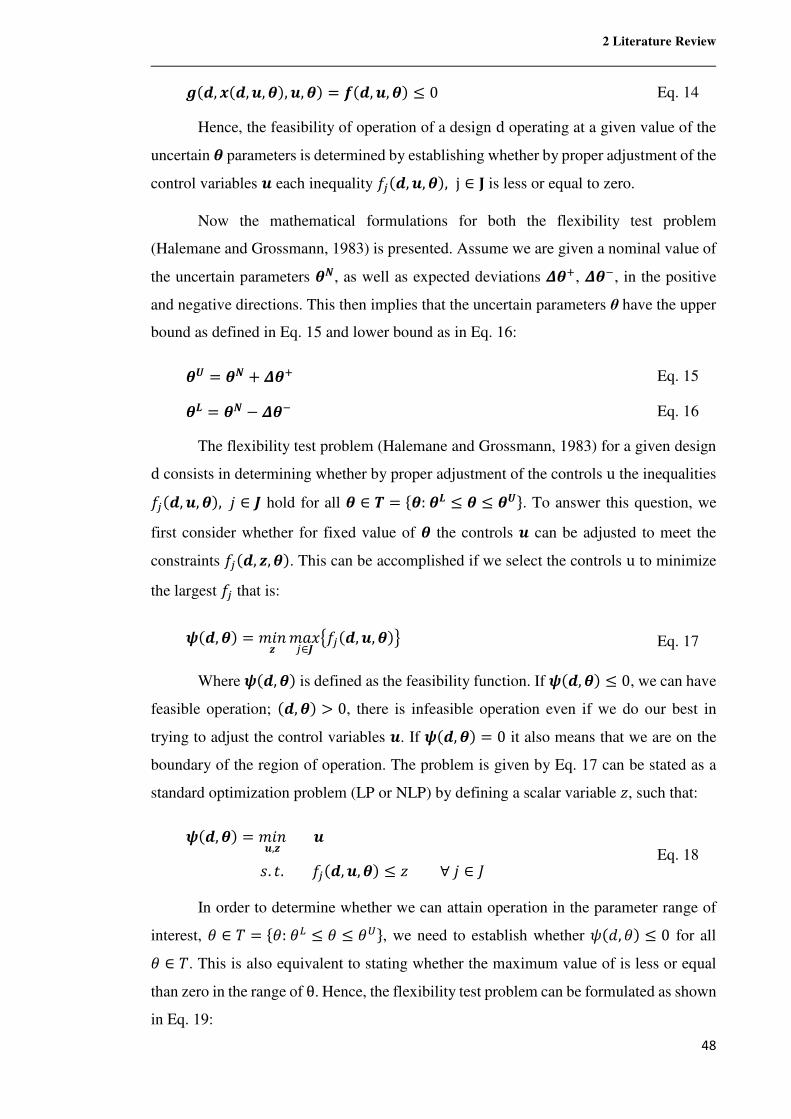
2 Literature Review
48
0k�, k�, �, [m, �, [m = Ük�, �, [m ≤ 0 Eq. 14
Hence, the feasibility of operation of a design d operating at a given value of the
uncertain [ parameters is determined by establishing whether by proper adjustment of the
control variables � each inequality +Ýk�, �, [m, j ∈ ß is less or equal to zero.
Now the mathematical formulations for both the flexibility test problem
(Halemane and Grossmann, 1983) is presented. Assume we are given a nominal value of
the uncertain parameters [¡, as well as expected deviations �[|, �[., in the positive
and negative directions. This then implies that the uncertain parameters θ have the upper
bound as defined in Eq. 15 and lower bound as in Eq. 16:
[g = [¡ + �[| Eq. 15
[` = [¡ − �[. Eq. 16
The flexibility test problem (Halemane and Grossmann, 1983) for a given design
d consists in determining whether by proper adjustment of the controls u the inequalities
+Ýk�, �, [m, à ∈ á hold for all [ ∈ ª = Ú[:[` ≤ [ ≤ [gÛ. To answer this question, we
first consider whether for fixed value of [ the controls � can be adjusted to meet the
constraints +Ýk�, ã, [m. This can be accomplished if we select the controls u to minimize
the largest +Ý that is:
®k�, [m = �¹Mã�~uÝ∈á
ä+Ýk�, �, [må Eq. 17
Where ®k�, [m is defined as the feasibility function. If ®k�, [m ≤ 0, we can have
feasible operation; k�, [m > 0, there is infeasible operation even if we do our best in
trying to adjust the control variables �. If ®k�, [m = 0 it also means that we are on the
boundary of the region of operation. The problem is given by Eq. 17 can be stated as a
standard optimization problem (LP or NLP) by defining a scalar variable æ, such that:
®k�, [m = �¹M�,ã
�
^. ¿.+Ýk�, �, [m ≤ æ∀à ∈ ; Eq. 18
In order to determine whether we can attain operation in the parameter range of
interest, ç ∈ è = Úç:çé ≤ ç ≤ ç8Û, we need to establish whether êkë, çm ≤ 0 for all
ç ∈ è. This is also equivalent to stating whether the maximum value of is less or equal
than zero in the range of θ. Hence, the flexibility test problem can be formulated as shown
in Eq. 19:
2 Literature Review
49
ìk�m = �~u[∈ª
äÜÕk�, [må Eq. 19
Where k�m corresponds to the flexibility function of design � over the range ª.
If k�m ≤ 0, it then means that feasible operation can be attained over the parameter
range Τ, and shown in the item a, Fig. 5. However, if k�m > 0 it means that at least for
part of the range of ª, feasible operation cannot be achieved (see item b, Fig. 5). Also,
the value of [that is determined in Eq. 19 can be regarded as critical for the parameter
range ª since it is the one where the feasibility of operation is the smallest (k�m ≤ 0) or
where maximum constraint violation occurs (k�m > 0).
Fig. 5 – Regions of feasible operation for feasible and infeasible design (flexibility test problem).
Finally, by substituting Eq. 17 in Eq. 19, the general mathematical formulation of
the flexibility test problem yields Eq. 20:
k�m = �~u[∈ª
�¹Mã�~uÕ∈á
+Ýk�, �, [m Eq. 20
Works based on these principles include the iterative methodology which has been
proposed in Bandoni et al. (1994) and Bahri et al. (1996) in order to analyse the steady-
state flexibility of a chemical plant. In this method, to ensure the feasible operation of the
plant, the optimum point is moved to somewhere inside the feasible region (called back-
off point). Therefore, having disturbances in the system will not cause any constraint
violation. The amount of back-off can be used as a measure of the flexibility of the plant.
Bahri, Bandoni and Romagnoli (1997) propose an integrated flexibility and
Controllability Analysis based on dynamic mixed-integer nonlinear programming that
2 Literature Review
50
consists of a two-stage problem for each iteration of the algorithm. These two stages are
called outer and inner loops, and each loop has been formulated as a semi-infinite
optimisation problem. Outer loops give the optimal operating conditions for a given set
of disturbances. In the inner loops, the feasibility of the operating conditions proposed in
the last outer loop is tested. In this stage, the disturbance realisations that produce most
constraint violations are found (if any) and passed to the next outer loop. In this way, the
authors claim, the effect of disturbances on the process design and operation, as well as
its ideal performance, under a variety of control schemes can be estimated. The method
is illustrated using a mini-integrated plant as a case study.
Bansal et al. (2000b) propose a parametric programming framework for feasibility
test, flexibility index, design optimization, and stochastic flexibility of linear systems,
providing an explicit information about the dependence of the system flexibility on the
values of the design variables. A case study of a double-effect distillation system (where
the overhead vapour from one column is used to supply the reboiler heat for another
column operating at a lower pressure), for which a dual approach is described: in the first,
the steady-state process design and the control system were optimised sequentially;
potential operability bottlenecks are identified. In the second approach, the process design
and the control system are optimised simultaneously leading to increased economic
benefit. Bansal et al. (2002a) generalise and unify this approach for the flexibility analysis
and design of nonlinear systems. Recent works dealing with flexibility evaluation are
Lima et al. (2010a,b), Chang et al. (2009) and Adi and Chang (2011).
2.1.1.4 Operability and Switchability Analysis
Operability is the ability of the plant to provide acceptable static and dynamic
operational performance. Operability includes flexibility, switchability, controllability
and several other issues. Switchability is the ability to switch between operating points.
For service plants, fast switching may be desirable to minimise loss of product and energy
consumption. Although controllability and flexibility are strongly related concepts
(Grossmann and Morari, 1984), controllability deals with the dynamic operation, and it
is a measure of the achievable dynamic performance, while flexibility is focused on the
steady-state operation and it is the capability to handle alternate operating conditions.
Dynamic feasibility is a commonly used term that encompasses both a static
aspect, which is incorporated into flexibility and a dynamic aspect, which is part of

2 Literature Review
51
switchability. The feasibility analysis problem is to determine if a given design can
feasibly operate over the considered range of uncertainty.
In Mohideen et al. (1996a) dynamic feasibility analysis is included in the
integrated design problem, verifying the operation and control constraints all over the
uncertainty range of the parameters in the established time horizon.
Bahri et al. (1996a, 1997) propose the dynamic operability analysis within the
process synthesis and control structure selection problem. This analysis includes aspects
as stability, controllability and flexibility; its objective is to optimise the process economy
subject to feasible regulatory dynamics. Stands out the use of the backwards margin based
on the dynamic nonlinear model. It relates the economic aspects with the operability, by
fixing the distance between the optimal steady-state operating point and the dynamic
operating point of the plant. They also consider the dynamic feasibility and indexes as the
ISE and the steady-state time. In Ekawati and Bahri (2003) this analysis is completed by
introducing the Output Controllability Index, OCI (Vinson and Georgakis, 2000).
In Novak Pintaric and Kravanja (2004) flexibility and static operability analysis
are introduced in the problem formulation by determining in a first stage, the optimal
flexible structure and optimal oversizing of the process units that guarantee feasibility of
the design for a fixed degree of flexibility. In a second stage, the structural alternatives
and additional manipulative variables are included in the mathematical model to
introduce additional degrees of freedom for efficient control. Malcolm et al. (2007)
contemplates the process and control design over a set of uncertain parameters by solving
the steady-state flexibility test and the dynamic flexibility test.
Vinson and Georgakis (2000, 2002) define the Output Controllability Index (OCI)
or Operability Index (OI) which is a steady state and nonlinear measure of the ability of
a design to reach all points of the desired output space and to reject the expected
disturbances using input actions not exceeding the available input space. It has been
proven to be effective for both linear and nonlinear processes. Its extension to a dynamic
analysis called Dynamic Operability Index (DOI) is presented in Uzturk and Georgakis
(2002). These operability analysis tools are exploited in Subramanian et al. (2001) for
examining the inherent steady state operability of continuous processes, using as an
example a CSTR system. They propose an approach that further extends the original OI
formulation to include nonsquare systems, distinguishing different categories for process
outputs: (1) set-point controlled, with outputs to be controlled at a desired value, and (2)
2 Literature Review
52
set-interval controlled, with outputs to be controlled within the desired range. In
Georgakis et al. (2003) a similar methodology is presented. An extension of the
operability analysis for plantwide systems is applied to the Tennessee Eastman process
in Subramanian and Georgakis (2005).
Psarris and Floudas (1991) claim that the location of Right-Half-Plane-
Transmission (RHPT) zeros is essential for the assessment of dynamic operability since
if RHPT zeros are close to the origin of the complex plane severe limitations are imposed
to the closed-loop performance of multivariable systems. The authors claim that in
multivariable systems with time delays, infinite transmission zeros may be present which
makes their numerical determination and therefore the assessment of dynamic operability
is very difficult. The methodology presented in Psarris and Floudas (1991) provides a tool
for assessment of dynamic operability of MIMO delay systems through the
characterisation of the transmission zeros by using the theory of the distribution of roots
of quasi-polynomials to identify systems with infinite RHPT zeros.
Other studies which develop strategies to incorporate controllability and
operability insights into the practice of process design include Grossmann and Morari
(1984), Grossmann and Floudas (1987), Grossmann and Straub (1991) and Dimitriadis
and Pistikopoulos (1995).
2.1.1.5 Disturbance Cost Index
Lewin (1996) presented the Disturbance Cost index, DC, a frequency-dependent
resiliency index defined as the control effort required in rejecting the worst-case
disturbance, intended to provide guidance as part of a modern process design
methodology. As most indexes, the DC represents a measure of the control effort (which
can be roughly defined as how much the controller needs to move manipulated variables
compared to their ranges) required to reject the worst-case disturbance, normalised to
enable comparison between different plants. The authors justified the introduction of this
index by discussing the incapability of the previously mentioned measures for quantifying
the disturbance resiliency properties of a linear process.
Let us assuming perfect disturbance rejection by the control system and a linear
dynamic model for the process. The norm of the actuator response computed,‖u‖, is a
function of the disturbance direction. The relative cost of rejecting a particular disturbance
d can be computed as a function of its direction, .i.e., a quantitative measure of the control
effort to reject a given disturbance vector is the Euclidean norm. Hence, this norm,‖u‖,
2 Literature Review
53
is defined as the Disturbance Cost. The DC index was extended by Solovyev and Lewin
(2002) to address nonlinear, state-space models.
Lewin and Bogle (1996) applied the DC index to perform the selection of the
optimal operating point for a continuous industrial polymerization reactor. For each
operating point, the DC contours were plotted as functions of disturbance frequency and
direction, yielding a graphical representation of the space of disturbance realisations the
control loop is able to reject.
A measure similar to the DC has been proposed in Narraway et al. (1991), which
presents a method to evaluate the impact of disturbances on plant economic performance
in alternative process structures or alternative control schemes for a given process. The
best operating point in the absence of disturbances is obtained by nonlinear steady-state
optimisation, and frequency response analysis of a linearized plant dynamic model is used
to estimate the effects of disturbances on this ideal performance under a variety of control
strategies. A modification of this method is presented in Narraway and Perkins (1993). In
this work, they provide a measure of the best achievable economic performance as the
amount that the operating point must be backed off from constraints active at the optimal
operating point to accommodate the effects of disturbances. The back-off idea is also used
to measure the effect of dynamical performance on economics because the required back
off represent the necessary extra cost to ensure that none of the operating constraints
which affect controllability is violated. Perfect control is assumed and integer
programming techniques are used for screening the potential control structures which are
then all subjected to controllability analyses or are used as control structures for nonlinear
dynamic economic analysis.
2.1.1.6 Disturbance Condition Number
The effectiveness of disturbance suppression in a multivariable control system can
depend strongly on the direction of the disturbance. Among the indexes proposed to
assess the resilience of chemical plants subject to disturbances, there is the method for
quantifying the effect of disturbance direction on closed-loop performance presented in
Skogestad and Morari (1987). There is a bound on the magnitude was obtained for the
worst-case relative gain by studying the direction of a disturbance, resulting in the
introduction of the Disturbance Condition Number (DCN). For a particular plant, the
DCN indicates the magnitude of the MV input magnitude necessary in order to
compensate for the effect of a disturbance of unitary magnitude in comparison to a
2 Literature Review
54
disturbance whose direction is the best possible. The “best” disturbance direction is the
one requiring the least action by the MVs. The Disturbance Condition Number is only a
good indication of which set-point vector will be difficult to track (Lewin, 1996).
2.1.1.7 Additional Controllability measures – the Relative Gain Array and Singular-
Value Decomposition
The singular values of a matrix are a measure of how close the matrix is to be
“singular”, i.e., to have a determinant that is zero. The N singular values of a real NxN
matrix A are defined as the square root of the eigenvalues of the matrix formed by
multiplying the original matrix by its transpose:
ð'µñ· = òÂ'µñóñ·,¹ = 1,… ,O Eq. 21
The minimum singular value was introduced as a controllability index by
Skogestad and Morari (1987), who suggested that a smaller minimum singular value
implies that large input magnitudes may be needed, and such plants are undesirable. The
SVD on G and Gr is useful for examining which manipulated input combinations have
the largest effect and which disturbances give the largest output variations. It can also be
used to predict directional sensitivity of a process. The process gain matrix is decomposed
into three matrices, as shown in Eq. 22:
/ = gi§jb Eq. 22
where Uõ is the left singular vector matrix, Σ the diagonal matrix of singular
values, ordered, and V the right singular vector matrix. The left and right singular vector
matrices are both orthonormal matrices, i.e., each column of the matrix is orthogonal to
all other columns, and the columns each are unit length. The diagonal singular value
matrix is ordered so that the largest singular value is in the (1, 1) position. Note that the
standard notation for SVD is to use U to represent the left singular vector matrix. When
performing singular value analysis, it is important to scale the inputs and outputs to cover
the same range.
“Condition number” is another important controllability index based on singular
value analysis. It is defined as the ratio between the largest singular value and the smallest
nonzero singular value. Plants with large condition number are called ill-conditioned and
require widely different input magnitudes depending on the direction of the desired output
2 Literature Review
55
(i.e. the plant is sensitive to unstructured input uncertain) (McAvoy and Braatz, 2003).
Note that the condition number is scaling dependent.
SVD can be used to assess just how well an algebraic process control problem is
posed and whether any sensitivity problems can be expected when it is solved. Early
application of SVD to process control systems was carried out by researchers at the
University of Tennessee (Downs and Moore, 1981; Moore, 1986). Lau et al. (1985) used
SVD to design multivariable control systems. Grosdidier et al. (1985) established a
quantitative relationship between the condition number of a process gain matrix and its
relative gain. Skogestad and Morari (1987) derived conditions for robust stability that
involved the condition number. A number of useful results on applying SVD to process
control problems are collected by Skogestad and Postlethwaite (1996). This includes the
result that saturation of the manipulated variable is a potential problem if the minimum
singular value of the process gain matrix is less than 1. They also show that the
multivariable effects of input uncertainties are small for processes with small condition
numbers. McAvoy and Braatz (2003) used SVD to analyse a process gain matrix,
focusing on the case where the process gain matrix has a large maximum singular value,
with its minimum singular value being either large or small. It is shown that the closed-
loop control of such processes can result in poor transient performance as a result of valve
accuracy considerations, even if the condition number is small and the minimum singular
value is large, which would indicate no performance limitations according to existing
controllability criteria.
Another widely used controllability measure is the RGA which was introduced by
Bristol, 1966. For instance, consider a plant defined by a square MIMO model /kim, as
shown in Eq. 6:
�kim = /kim�kim Eq. 23
The relative gain array is defined as the ratio of process gain as seen by a given
controller with all other loops open to the process gain as seen by a given controller with
all other loops closed and can be computed by Eq. 7:
£kim = /kim⨂÷/.�kimøb Eq. 24
where the ⨂ symbol indicates element-by-element multiplication (Schur
product). An important property of the RGA is that it is scaling independently. The
elements in the RGA can be numbers that vary from very large negative values to very
2 Literature Review
56
large positive values. The larger the values of the elements of RGA, the more sensitive
the transfer function will be in relation to errors. The closer the number is to 1, the less
difference closing the other loop makes on the loop being considered. For interactive
plants which do not have large RGA elements, a decoupler may be useful. In particular,
this applies to the case where the RGA-elements vary in magnitude with frequency, and
it may be difficult to find a good pairing for decentralised control (Skogestad and Hovd,
1990). The problem with pairing in order of avoiding interaction is that the interaction is
not necessarily always the undesirable thing. Therefore, the use of the RGA to decide
how to pair variables is not an effective tool for Controllability Analysis. In Barton et al.
(1992), the controllability of plant designs previously obtained by economic optimisation
of stationary models is evaluated, the steady-state Relative Gain Array is used to
determine the best input-output pairings, and the limitations to the functional
controllability are analysed. Then, the designs are modified in order to improve their
deficiencies.
The RGA and the determinant of the gain matrix provide useful information about
integral controllability and integrity (e.g., failure tolerance), which are important issues
in decentralised control. The RGA also gives information about robustness with respect
to modelling errors and input uncertainty. Based on these interesting properties,
Häggblom (2008) used the RGA to consider model uncertainty explicitly and thus
investigate the integral controllability and integrity of uncertain systems.
2.1.2 Process-Oriented Methods for Controllability Analysis
Several approaches where systematic actions are taken to improve some
controllability measures of plant performance and economic indicators have appeared in
the literature. They screen preliminary alternatives either by constraining some
controllability indicators or by optimising them, allowing the process or control design to
be carried out accordingly. Since the stated optimisation problems allow for the
consideration of process and control specifications as well as constraints, these methods
are used for accommodating decision variables within a unique integrated-optimisation
framework to solve both process design and the control-systems design (Perkins and
Walsh, 1996).
Among the opening contributors for controllability assessment and its
incorporation into process synthesis and the selection of the control structure, Morari and
Stephanopoulos (1980) discuss the structural design of alternative regulatory control
schemes to satisfy a posed objective. They use structural models to describe the

2 Literature Review
57
interactions among the units of a plant and the physicochemical phenomena occurring in
the various units. They discuss the relevance of controllability and observability in the
synthesis of control structures and use modified versions to develop all the alternative
feasible regulatory structures in an algorithmic fashion. Various examples are presented
to illustrate the developed concepts and strategies, including the application of the overall
synthesis method to an integrated chemical plant.
Marselle et al. (1982) present a heat exchanger network synthesis technique that
takes into account aspects of flexibility and resiliency, leading to networks flexible to
changes in the plant operating conditions. The method involves the structural and
parametric design of the network and the synthesis of the regulatory control structure.
The objective is to find the structure able to operate feasibly in a specific range of
uncertain parameters while achieving the maximum energy recovery. Saboo and Morari
(1984) develop a rigorous synthesis technique based on the fundamental properties for
maximum energy recovery in heat exchanger systems which leads to networks that can
handle specific inlet temperature variations and also guarantee maximum energy
recovery. In Morari et al. (1985) these techniques are extended to the synthesis of the heat
exchanger network and the control structure for a sequence of two exothermic open-loop
unstable continuous stirred tank reactors.
Modern chemical plants are highly integrated and interconnected which invariably
introduce a dynamic coupling between the process units. Material and energy recycle
affects process performance leading to complex dynamic behaviours, such as inverse
response, open loop instability and unexpected behaviour. Among the several authors
who proposed strategies to quantify the impact of such effects on controllability, we may
highlight Denn and Lavie (1982), Morud and Skogestad (1994), McAvoy and Miller
(1999), Jacobsen (1997), Dimian et al. (1997), Semino and Giuliani (1997), Bildea and
Dimian (2003), Lakshminarayanan (2004) and Bildea et al. (2004).
Zheng and Mahajanam (1999) have pointed out that there are very few indices
available which establish a direct relationship between cost and controllability. They
propose an index to quantify the cost associated with dynamic controllability of a process
with a given control structure, focusing on the additional surge volume (or overdesign)
required to achieve the control objectives. Such cost/controllability index is used to
quantify the cost associated with dynamic controllability. Establishing a relationship
between capital costs and controllability as a way to monetise control performance is an
2 Literature Review
58
interesting idea, and closely related to the motivation of this PhD project. However, here
we place focus instead on operating costs and plant revenue.
Along similar lines, Zheng et al. (1999) propose a hierarchical procedure where
alternative plantwide control systems are synthesised and compared regarding economics.
They describe the design procedure for an existing plant (a simple reactor-separator-
recycle system) and also show how the interesting problem of determining the optimum
surge capacities of a process can be addressed through simple modifications.
We may also highlight works such as Stephanopoulos et al. (1979), Morari et al.
(1980), Morari et al. (1987) and the series “Design of Resilient Processing Plants”
(Lenhoff and Morari, 1982; Marselle et al., 1982; Morari, 1983; Saboo and Morari, 1984;
Holt and Morari, 1985a,b; Morari et al., 1985; Saboo et al., 1985; Skogestad and Morari,
1987).
2.1.2.1 Controllability Analysis of Systems with Recycles
Luyben and co-workers present a series of papers devoted to the study of
dynamics and control of recycling systems in chemical processes (Luyben, 1993a, 1993b,
1993c, 1994, 1999; Tyreus and Luyben, 1993). The special dynamic behaviour of
recycling systems, identified in the works just mentioned, are important in the
development of process design methodologies, in the subsequent works of the authors.
Particularly, Elliott and Luyben (1995) present a capacity-based economic approach
which allows comparing and screening quantitatively conceptual plant designs assessing
both, steady-state economics and dynamic controllability of the process.
The alternative plant designs are evaluated considering their ability to maximise
annual profit in the presence of their associated peak disturbances. The method deals
explicitly with the impact of product quality variability on plant profits, considering the
losses generated in the fraction of the time that the product is outside the limits of desired
specifications. A reactor/stripper recycle system is considered as a case study. The
methodology is applied in the design of a complex recycle system consisting of one
reactor and two distillation columns in Elliott and Luyben (1996). In this case study, the
approach is used to design parameter alternatives, conceptual design flowsheet
alternatives, and control structure alternatives for the system.
Luyben and Luyben (1996) deal with the plantwide design and control of a
complex process containing two reaction steps, three distillation columns, two recycle
flows and six chemical components. A heuristic design procedure and a nonlinear
2 Literature Review
59
optimisation are used to determine an approximate economically optimal steady-state
design; the sensitivity to design parameters and specifications is evaluated and control
strategies are developed using guidelines from previous plantwide control studies. In
Luyben (2000), the trade-off between the reactor size, recycle flow rate and reactor inlet
temperature of a gas-phase reactor/recycle plant in the steady-state design is studied, as
well as the economic impact of inert components in the feed stream. In a second step,
alternative control structures are evaluated and basic control strategies are applied in the
presence of large disturbances. Reyes and Luyben (2000) present a similar study for an
irreversible reaction system with a reactor feed preheating system (feed-effluent heat
exchanger and furnace) where the steady-state economics and the dynamic controllability
of this dual-recycled system are compared with those of single-recycle processes. Both
Reyes and Luyben (2001a) and Reyes and Luyben (2001b) focused on processes with
realistic separation systems (a distillation column) for gas-phase tubular reactors with a
liquid recycle and with a dual recycle system.
Other contributions are found in the works of Cheng and Yu (2003) and Kiss et
al. (2005). The former explores the dynamics of simple recycle plants under different
process designs using different control structures. The recycle dynamics is evaluated
using transfer-function-based linear analysis and also validated using rigorous nonlinear
simulation; finally, implications to control structure design are specified for different
levels of reactor conversions. Kiss et al. (2005) address the design of recycling systems
involving multiple reactions. They use the mass balance model of the plant to capture the
interaction between units and to predict the main pattern of behaviour. After choosing the
method of controlling the plantwide material balance, the nonlinear analysis reveals
regions of infeasibility, high sensitivity, state multiplicity, and instability.
2.1.2.2 Controllability Analysis Based on Steady-State Multiplicity Analysis
Input multiplicities occur when more than one set of manipulated variables (MVs)
can produce the desired steady-state output (CVs). Multiplicities are related to the
stability and desirability of any intended loop pairing of MVs and CVs. The danger under
the existence of input multiplicities is the undetected transition from one steady-state to
another. It is thus a good policy to examine the steady-state behaviour to detect
multiplicities since the possibility of an undetected transition to an unanticipated, and
perhaps economically undesirable, the steady-state operating condition is best eliminated
at the system design stage (Koppel, 1982).
2 Literature Review
60
Some interesting works are focused on integrating operability criteria into
chemical reactors design based on the steady state multiplicity analysis. Several
preliminary results by Russo and Bequette (1995, 1996, 1997, 1998) use the bifurcation
based approach to study the behaviour of CSTRs showing that the infeasible operation
regions that affect open loop and closed loop performance can be avoided with some
parameter modifications in the design stage. More recently, Altimari and Bildea (2009)
tackle the integrated design and control of plantwide systems. Their methodology
evaluates the steady-state multiplicity and allows selecting possible flowsheets and
admissible control structures regarding feasibility. Guidelines are derived which enable
the selection of reactor parameters in a way that guarantees wide margins of plant
operating conditions from infeasibility boundaries. While thorough analysis is provided
on the interaction between reactor design and plant operability, no connection to process
economics is discussed. In the current project, we wish to link the idea of steady-state
multiplicity to operating cost and revenue.
The influence of input/output multiplicity on stability and non-minimum phase
behaviour of chemical reaction systems is studied in Yuan et al. (2009), Yuan et al.
(2011), Wang et al. (2011) and Wang et al. (2013). With a focus on inherently safer
designs, their study reveals how the essential properties of a process change with
variations in its operating conditions. A systematic framework that includes multiplicity
and phase behaviour together with open loop stability analysis over the entire feasible
operation region of plantwide processes is presented in Yuan et al. (2012b).
Yuan et al. (2009), address a strategy for classifying the process operating region
into distinct zones at the early stage of process design, based on stability/instability and
minimum/non-minimum phase behaviour analysis. Ma et al. (2010) presented an
approach using continuation and optimisation methods for modifying a process design to
avoid the issues caused by input multiplicity. Wang et al. (2011) conclude that stability
and phase behaviour should be analysed considering the overall system rather than
individual units because those properties may differ from the global system. Yuan et al.
(2011) present a methodology that explores the open and closed-loop controllability of
the liquid-phase catalytic oxidation of toluene. They evaluate set-point tracking and
disturbances rejection in various sub-regions with different controllability characteristics.
2 Literature Review
61
2.1.2.3 Controllability Analysis Based on Phenomenological Models and the Passivity
Theory
Put together in this section are the procedures where the phenomenological
knowledge of the process is used to distinguish the designs with best dynamic
performance, using sensibility analysis of thermodynamic properties or, specifically, the
passivity theory.
In fact, several works can be found in the literature that takes advantage of
mathematical models and thermodynamic properties of a process to improve process
synthesis, integrating sensitivity to perturbations and other control aspects. In Gani et al.
(1997), different process flowsheets and equipment design parameters are generated
through simulations using simple or rigorous models of the process, analysing at every
step different process features, and including environmental aspects and controllability.
In Russel et al. (2002), more emphasis is given to the analysis of the process model as a
preliminary solution step for integration of design and control problems. In Li et al.
(2003), a systematic sensitivity analysis of the process model is developed to select the
best control structure. In Ramirez Jimenez and Gani (2007a,b), a model based analysis
methodology for the integrated design and control is presented, using first-principles
phenomenological models of different complexities to identify the interactions between
the process and design variables. Parametric sensitivity analysis is performed to
determine the control structure.
In Hamid et al. (2010) the simultaneous process and control system design of a
process is addressed by the reverse design algorithm approach. The formulation of the
integrated optimisation process design and process control problem is decomposed in four
subproblems easier to solve. The search space is reduced by considering thermodynamic
and feasibility aspects, the concepts of the attainable region (AR) and driving force (DF)
are used to locate the optimal process-controller design in terms of the optimal condition
of operation from design and control viewpoints. The AR concept is used to find the
optimal (design target) values of the process variables for any reaction system. The DF
concept is used in this methodology to find the optimal (design target) values of the
process variables for separation systems. The final selection and verification are
performed according to the value of the objective function. Alvarado-Morales et al.
(2010) extend this methodology, proposing a framework that combines the simultaneous
process design and controller design methodology and the process-group contribution
(PGC) methodology. A process flowsheet can be described by means of a set of process-
2 Literature Review
62
groups bonded together to represent the structure. The PGC methodology has been used
to generate and test feasible design candidates based on the principles of the group-
contribution approach used in chemical property estimation. It is applied to the bioethanol
production process; however, this is a general framework that can be applied to different
processes.
A category of process control algorithms based on thermodynamic-models was
proposed in Ydstie and Viswanath (1994) and incorporated in the Integrated Process and
Control Design Framework by Meeuse et al. (2000, 2001), Meeuse (2002) and Meeuse
and Grievink (2002). These works embed Controllability Analysis within the process
synthesis, assessing sensitivity to perturbations by means of the passivity theory.
A passive component may be either a component that consumes (but does not produce)
energy (thermodynamic passivity) or a component that is incapable of power
gain (incremental passivity). Passivity is then a property that can be used to demonstrate
that passive passivity systems will be stable under specific criteria. The passivity systems
are a class of processes that dissipate certain types of physical or virtual energy, defined
by Lyapunov-like functions. The authors use the passivity framework, linked to process
thermodynamics, in process input-output Controllability Analysis. This approach allows
for studying the stability of distributed systems and the selection of the manipulated and
measured variables pairing alternatives that ensure stability and efficient plant operation
by relating the entropy production sensibility of the plant with its sensibility to
perturbations. Specifically, in Meeuse (2002) and Meeuse and Grievink (2004),
controllability conditions are incorporated in the process synthesis by considering
thermodynamic aspects of the process, to derive some design guidelines.
2.1.3 Integrated Process Design and Control Framework - Methods of Integrated
Control and Process Synthesis
This section will focus on the available methods of Integrated Control and Process
Synthesis, the second class of methods defined in Lewin (1999). Works that fall into this
classification are used to generate process flowsheets, embedding Controllability
Analysis in the process synthesis. Different operability and sensitivity qualities are and
explored to determine plantwide process structure, and also to provide insight into control
system design.
The dynamic performance measures are introduced in the process design,
originating a single optimisation scenario which may additionally contain the tuning of
2 Literature Review
63
the controllers and even the selection of the control structure. The formulation of the
optimisation problem contains decision variables, objective functions and constraints
related to economics as well as operating and control performance aspects. Thus, this
approach provides the possibility of carrying out at once the process and the control
system design by solving the optimisation problem, providing the plant design that best
satisfies the compromise between economic and control aspects and all the criterion
considered in the problem formulation.
Pioneering works that introduced the idea of integrating the process design and
the controllability issues in a comprehensive optimisation problem were those by Lenhoff
and Morari (1982), Palazoglu and Arkun (1986) and Georgiou and Floudas (1990),
among others. In Lenhoff and Morari (1982) an optimisation based design approach
considering economic and dynamic aspects simultaneously is proposed, taking into
account process structural decisions, parametric changes and the control structure
selection which leads to a multiobjective optimisation problem. Georgiou and Floudas
(1990) developed a systematic framework for control system synthesis. They used the
generic rank of a process structural matrix as an index of structural controllability to select
the best process configuration, computed by solving an integer-linear optimisation
problem.
Perkins and Walsh (1996) pointed out the notable trend towards the use of
optimisation as a tool for the integration of process design and process control, which was
enabled by advances in computational hardware and optimisation methods and driven by
the need to place control design decisions on the same basis as process design decisions.
2.1.3.1 The Integrated Control and Process Synthesis Problem
A complete formulation of the integrated design of a process includes in addition
to the determination of the plant dimensions and operating conditions, the selection of the
plant topology (process synthesis) and the selection of the control structure (input-output
pairing and control scheme). When the process synthesis is considered, the optimisation
problem is posed based on a superstructure containing all the possible alternatives of the
process (algorithmic synthesis or automatic synthesis), aimed to find the optimal
flowsheet in the economic and controllable sense. The selection of the control system
configuration can also be embedded in a superstructure. This formulation involves
continuous variables, representing the dimensions and operating conditions, and discrete
variables, related to the process/controller structure.
2 Literature Review
64
As both discrete and continuous variables are embedded into this problem, it can
be formulated naturally as a mixed-integer dynamic optimisation (MIDO) problem. The
integer variables take care of discrete decisions (i.e. flowsheet structure, the number of
control loops, the number of distillation columns, etc.), while the continuous variables are
normally related to design variables (i.e. flows, temperatures, composition, etc.). As many
chemical processes feature nonlinear behaviour around optimal design regions, it is likely
that the MIDO problem gives rise to a nonlinear optimisation formulation.
Walsh and Perkins (1996) and Narraway and Perkins (1993) were among the first
to consider general mathematical programming techniques for the simultaneous synthesis
and control problem using dynamic process models, proposing methods that possess an
explicit economic component was presented for optimal plant design involving a classical
feedback control structure. In practice, similar approaches involve attributing a cost to a
control performance measure such as the integral error, e.g., ISE or IAE, performing a
worst-case design optimisation for tuning one or more PID controllers for optimal system
response and then varying a number of equipment design parameters, then repeating the
process until the global solution is found. This avoids equipment oversizing and thus
decreases costs. Dimitriadis and Pistikopoulos (1995) applied the ideas reported in
Halemane and Grossmann (1983) to systems described by sets of differential and
algebraic equations.
Different formulations of the integrated design including the process synthesis and
the selection of the control structure are found in the literature. Luyben and Floudas
(1994a) present a general formulation of the problem considering a superstructure for the
process synthesis that includes all possible design alternatives of interest and open-loop
steady-State Controllability measures. Mohideen et al. (1996a) propose a unified process
synthesis optimisation framework for obtaining process designs together with the control
structure and controller design under uncertainty. The objective is to design the process
and the required control scheme at a minimum total annualised cost which comprises
investment and operating costs including controller costs. It results in an optimum set of
design variables, the best selection/pairing of controlled-manipulated variables and the
optimal values of the controller parameters. Similar formulations and solution procedures
were reported in Bahri, Bandoni and Romagnoli (1997) and Schweiger and Floudas
(1999). The main drawback of these methodologies stems from the fact that the combined
design and control problem, a mixed-integer dynamic optimisation (MIDO) problem, is
solved as a mixed integer nonlinear programming (MINLP) problem by transforming the
2 Literature Review
65
system of differential and algebraic equations into algebraic equations by using either full
discretisation or integration. In the former case, the size of the resulting MINLP is
explosive, and in the latter case, extensive dual information is needed to formulate a
(mixed integer linear) master problem that is ever increasing in size.
The Mixed-Integer Dynamic Optimisation algorithms reported in the literature are
based on complete discretisation (Mohideen et al., 1996a), on an adjoint-based approach
(Sakizlis et al., 2001), and on an outer approximation (Bansal et al., 2003). None of these
methods are guaranteed to find the exact global optimum of the underlying optimisation
problem. Therefore, the need for new global mixed-integer dynamic optimisation
algorithms becomes extremely important in preventing the generation of economically
unfavourable designs.
Some other works addressing the complete integrated design problem involving
closed-loop behaviour analysis into the optimisation are Mohideen et al. (1996b), Bahri
et al. (1996a), Bansal et al. (2000a), Kookos and Perkins (2001), Ekawati (2003), Flores-
Tlacuahuac and Biegler (2007) and Revollar et al. (2012). Angira (2005), Angira and
Alladwar (2007), Babu and Angira (2006), Angira and Babu (2006) used evolutionary
solution methods for solving the nonlinear, mixed integer nonlinear and dynamic
optimisation problems encountered in chemical engineering. But these techniques are not
applied and tested on Mixed-Integer Dynamic Optimisation problems that arise from the
simultaneous process design and control. Sánchez-Sánchez and Ricardez-Sandoval
(2013a), Trainor et al. (2013) and Sharifzadeh and Thornhill (2013) also develop fully
integrated process synthesis and control formulations.
A number of works carry out the integrated design considering only the process
synthesis and the determination of the optimal plant dimensions, operating conditions and
even the controller parameters: Schweiger and Floudas (1997), Bahri et al. (1997),
Gutierrez (2000), Sakizlis et al. (2003, 2004), Malcolm et al. (2007), Revollar et al. (2008)
and the recent contributions of Revollar et al. (2010a), Revollar (2011) and Sánchez-
Sánchez and Ricardez-Sandoval (2013b). Some other works focus on process
dimensioning and determination of optimal operating conditions including the selection
of the control structure and controller tuning: Narraway and Perkins (1994), Asteasuain
et al. (2005, 2006, 2007), Patel et al. (2007) and Flores-Tlacuahuac and Biegler (2008).
Other works considering fixed structures are Lenhoff and Morari (1982),
Palazoglu and Arkun (1986), Luyben and Floudas (1994b), Gutiérrez and Vega (2000),
Blanco and Bandoni (2003), Chawankul et al. (2007), Miranda et al. (2008), Grosch et al.
2 Literature Review
66
(2008), Kim and Linninger (2010), Francisco et al. (2011) and Ricardez-Sandoval (2012).
Large scale systems are addressed in recent works as Exler et al. (2008), Moon et al.
(2011), Ricardez-Sandoval et al. (2009c, 2010, 2011) and Munoz et al. (2012).
2.1.3.2 Integrated Control and Process Synthesis with Guaranteed Robust Performance
A fundamental question about control algorithms is its robustness to model
uncertainty and noise. When we say that a control system is robust we mean that stability
is maintained and that the performance specifications are met for a specified range of
model variations and a class of noise signals (uncertainty range). To be meaningful, any
statement about “robustness” of a particular control algorithm must make reference to a
specific uncertainty range as well as specific stability and performance criteria.
The robust control framework makes use of a terminal cost that is also a Control
Lyapunov Function for the system. Control Lyapunov Functions (CLFs) are an extension
of standard Lyapunov functions and were originally introduced by Sontag (1983). CLF is
a Lyapunov function Vkxm for a system with control inputs. They allow the constructive
design of controllers and the Lyapunov function that proves their stability. The ordinary
Lyapunov function is used to test whether a dynamical system is stable (more
restrictively, asymptotically stable). That is, whether the system starting in a state x ≠ 0
in some domain D will remain in D, or for asymptotic stability will eventually return to
x = 0. A CLF, however, is used to test whether a system is feedback stabilizable, that is
whether for any state x there exists a control ukx, tm such that the system can be brought
to the zero state by applying a control action u. Consider a nonlinear control system x¼ =fkx, um, where x ∈ ℝýþ and u ∈ ℝý� . The following definition is valid.
Definition 2.1.3.2.1 Control Lyapunov Function. A locally positive
function j ∶ ℝMu → ℝ+ is called a Control Lyapunov Function (CLF) for a
control system if Eq. 25 is valid.
∀ ≠ 0,∃� ¹M+ ��j�� +k, �m� < 0 Eq. 25
Eq. 25 is a key condition; it says that for each state we can find a control � that
will reduce the magnitude of j. Intuitively, if in each state we can always find a way to
reduce the j, we should eventually be able to bring the j to zero, that is to bring the
system to a stop. This is made rigorous by the following result:
2 Literature Review
67
Artstein's theorem. The dynamical system has a differentiable control-
Lyapunov function if and only if there exists a regular stabilizing
feedback �km.
A complete treatment is given in Krstic (1995). In general, it is difficult to find a
CLF for a given system. However, for many classes of systems, there are specialized
methods that can be used. One of the simplest is to use the Jacobian linearization of the
system around the desired equilibrium point and generate a CLF by solving a Linear–
Quadratic Regulator (LQR) problem. The problem of minimizing a quadratic
performance index, Eq. 26, subject to ¼ = � + �� and k¾m = ¾, results in finding
the positive definite solution of the Riccati equation, P, Eq. 27:
; = ÷bk¿mUk¿m +�bZ�k¿møë¿�B Eq. 26
�bR + R� − R�Z.��bR + U = 0 Eq. 27
where Z is the factor of input suppression and U is the LQR weight. The optimal
control action is given by Eq. 28:
� = −Z.��bR Eq. 28
where j = bR is a CLF for the system. In the case of the nonlinear system
¼ = +k, �m, � and � are taken as:
� = � k,�m� �kB,Bm
Eq. 29
� = � k,�m�� �kB,Bm
Eq. 30
The CLF jkum = bR is valid in a region around the equilibrium k0,0m. More
complicated methods for finding control Lyapunov functions are often required and many
techniques have been developed. An overview of some of these methods can be found in
Jadbabaie (2001).
In the recent years, robust approaches using CLFs have been introduced in the
integrated process design and control formulations. They consider the uncertainties
existing in real processes to provide robustness properties to the obtained plants and the
worst-case variability. In these approaches, the process nonlinear dynamic model is
2 Literature Review
68
represented as uncertain models that can be used to calculate bounds on the variables that
are involved in the objective function and the constraints of the problem under
consideration (Ricardez-Sandoval et al., 2010).
In many works, the effects of uncertainties and perturbations are ignored or else
very simple perturbations profiles are considered (Narraway and Perkins, 1994;
Schweiger and Floudas, 1997; Bahri, 1996; Kookos and Perkins, 2001). Nevertheless, in
Bandoni et al. (1994) an algorithm for the worst-case is presented, to compute the
maximum variation of the uncertain parameters that can take place without impairing the
feasibility of the process. Another group of publications can be found, focused on
studying the effects of different settings of perturbations and parameter uncertainties on
the process economics and dynamic performance (Mohideen et al., 1996a, 1996b; Bahri
et al., 1996b, 1997; Bansal et al., 2000a; Asteasuain et al., 2007).
In Chawankul et al. (2007) robust integrated design has been developed,
particularly quantifying the uncertainties as a family of linear models around the nominal
model. These uncertain models have been typically used in robust control, and they have
also been used for integrated design in Francisco et al. (2011). However, most of the
robust integrated design methods consider parametric uncertainty. In Moon et al. (2011)
some uncertain scenarios are considered varying process parameters. In Munoz et al.
(2012), an extension of the normal vector method is developed to consider simultaneously
disturbances and uncertain model and process parameters. Ricardez-Sandoval et al.
(2009a) consider model parametric uncertainty that is translated to an uncertain state-
space model. In this study, uncertain dynamic models of the process, obtained from the
nonlinear dynamic closed-loop process model, were used to estimate analytical bounds
on the worst-case variability and the process feasibility constraints. The bounds were
computed using a formulation introduced by the authors based on a Structured Singular
Value analysis named ‘Analytical Bounds Worst-case Approach’ (BWA). Later this
approach was extended to a robust Finite Impulse Response model with uncertain
parameters (Ricardez-Sandoval et al., 2009b, 2009c, 2010). In Ricardez-Sandoval et al.
(2011), the uncertainty of process physical parameters was addressed. Sánchez-Sánchez
and Ricardez-Sandoval (2013a,b) include process synthesis and control structure
decisions, but using again the uncertain Finite Impulse Response model.
As for the treatment of disturbances, Chawankul et al. (2007) only consider
sinusoidal time-varying disturbances, and Gerhard et al. (2005) and Monnigmann and
Marquardt (2005) are also limited to particular disturbances. Other works consider a
2 Literature Review
69
general form of the disturbances, by means of their maximal magnitude. Particularly,
Ricardez-Sandoval et al. (2008, 2009a, 2009b, 2009c, 2010, 2011) assume general
disturbances of bounded magnitude, carefully calculating the worst-case disturbance.
Francisco et al. (2011) also consider the maximal magnitude of the disturbances based on
the actual weather profiles.
In Monnigmann and Marquardt (2005) a method is proposed that establishes
robust measures based on a minimal distance between the uncertain parameter space
region and the critical boundaries. Later, in Grosch et al. (2008), constraints are imposed
simultaneously on time-domain performance indicators and the asymptotic dynamic
process behaviour while optimising the steady-state profit of the plant, accounting for the
effect of uncertainty in both, design and model parameters. This approach is difficult to
apply in the presence of more than one disturbance, then, to overcome its disadvantages.
Munoz et al. (2012) use an extension of the normal vector approach proposed in
Monnigmann and Marquardt (2002) to consider the simultaneously robust asymptotic
stability of steady states despite parametric uncertainty and robust feasibility of the
transient behaviour despite disturbances.
In particular, several articles by Ricardez-Sandoval and co-workers present a
robust approach based methodology that performs the simultaneous design and control
under disturbances and process model parameters uncertainties. In Chawankul et al.
(2007) a measure of the closed loop output performance is introduced based on the output
widest variability caused by model uncertainties and constraints related to the robust
stability of the plant imposed. Furthermore, this performance index is added to the
objective function as a cost associated with the variability. In Ricardez-Sandoval et al.
(2008, 2009a, 2009b) a new technique is presented to assess the flexibility, stability and
controllability of a process. In this method, the infinite time horizon bounds are estimated
for the worst-case scenarios, enforcing process feasibility constraints by using the
Structured Singular Value Analysis (SVA), avoiding expensive dynamic optimisations.
This methodology is improved in Ricardez-Sandoval et al. (2009c) to reduce the
computational requirements of the method towards its application to large-scale
processes; the methodology is referred as the Analytical Bounds Worst-case Approach
(BWA). However, a disadvantage of this approach is the conservatism resulting from the
use of analytical bounds. In Ricardez-Sandoval et al. (2010) a method named Hybrid
Worst-Case Approach (HWA) is proposed. It combines the analytical calculation of the
worst-case disturbance and dynamic simulations using the mechanistic closed-loop
2 Literature Review
70
process model to calculate variability. It is expected to reduce the conservatism in the
final design at the expense of additional computational time in the calculations. Ricardez-
Sandoval et al. (2011) have expanded hybrid worst-case approach considering time-
varying disturbances and parametric model uncertainties, making it suitable for
application to large-scale systems.
In Sánchez-Sánchez and Ricardez-Sandoval (2013a) is presented a method for
optimal process synthesis and control structure selection that simultaneously evaluates
dynamic flexibility and dynamic feasibility in the presence of the worst-case (critical)
time-trajectories in the disturbances. Furthermore, a robust stability test based on
Quadratic Lyapunov theory is included in this methodology to ensure that the optimal
design is asymptotically stable for any of the magnitude-bounded perturbations
considered in the analysis. The disturbances are treated as stochastic time-discrete
unmeasured inputs. The work of Trainor et al. (2013) adopts this methodology for the
design of a ternary distillation system treating disturbances as random time-dependent
bounded perturbations. It presents a methodology for the optimal process and control
design of dynamic systems under uncertainty that incorporates robust feasibility and
stability analyses formulated as convex mathematical problems. This approach is
computationally attractive since it does not require the solution of a MINLP. A norm-
bounded metric based on Structured Singular Value (SSV) analysis is employed to
estimate the worst-case deviation in the process constraints in the presence of critical
realisations in the disturbances.
In Gutierrez et al. (2013) an integrated design methodology focused on the
selection of an optimal control structure is addressed by adding a communication cost
function within the overall cost function. Different control structures composed of
centralised and fully decentralised predictive controllers are considered in the analysis. A
cost function related to the worst-case closed-loop variability is calculated using
analytical bounds derived from tests used for robust control design.
In Matallana et al. (2011) a design methodology based on the optimisation of the
domain of attraction is proposed. The idea is to simultaneously ensure asymptotic stability
and an optimum domain of attraction of the resulting operating point in a certain sense.
The approach consists of maximising the radius of a ball in the state's space within which
negative definiteness of the time derivative of a quadratic type Lyapunov function can be
ensured.
2 Literature Review
71
In Francisco et al. (2011) and Francisco (2011) norm based indexes for
controllability are considered. They allow for including robust performance conditions
within the integrated design procedure by using a polyhedral uncertainty region, limited
by multiple linearized models. The multiobjective problem stated include investment,
operating costs, and dynamical indexes based on the weighted sum of some norms of
different closed-loop transfer functions of the system.
2.1.3.3 Probabilistic Based Integrated Control and Process Synthesis Methods
Some of the recent works presented in the literature for optimal design considers
a stochastic or probabilistic-based approach. Most of the design procedures ensure the
appropriate process performance in the presence of uncertainties and disturbances
focusing on the worst-case scenario given by the critical realisations in the disturbances
and the uncertain system’s parameters that produce the largest deviations in the controlled
variables, demanding major control efforts to maintain the desired operating conditions.
This is called the worst-case process variability (Bahakim and Ricardez-Sandoval, 2014).
The overestimation of the uncertainties, typical in process design methodologies, leads to
conservative design decisions resulting in an unnecessary deterioration of the objective
function, In such sense, probabilistic programming is a promising solution for solving
optimisation problems under uncertainty in the process industry (Li et al., 2008) allowing
to take into account the probability of occurrence of the worst-case variability in the
process variables.
Few works have introduced such considerations in the integrated design
formulation. Ricardez-Sandoval (2012) introduces a distribution analysis on the worst-
case variability in the integrated design framework. The worst-case variability is
approximated by normal distribution functions to estimate the largest variability expected
for the process variables at a user-defined probability limit. Thus, the user can rank the
goals of the design according to its particular criterion. The worst-case variability
estimates are used to evaluate the process constraints, the system’s dynamic performance
and the system’s cost function enabling the assessment of the optimal process design by
assigning different probability levels to the process variables used to evaluate the process
constraints and the process economics. In Bahakim and Ricardez-Sandoval (2014) an
optimisation framework for achieving a feasible and stable optimal process design in the
presence of stochastic disturbances while using advanced model-based control scheme is
proposed.
2 Literature Review
72
2.1.3.4 Examining the Control Structures used in Integrated Control and Process
Synthesis
In several formulations of the integrated optimisation of process design and
control the controller parameters are introduced as decision variables in the optimisation,
while in others they are tuned empirically. Some formulations focus in the analysis of the
open loop system to obtain an optimal and controllable design for any possible controller,
as in Luyben and Floudas (1994a), Grosch et al. (2008), Matallana et al. (2011) and
Guerra et al. (2012). In some works, the notion of perfect control is assumed in the
optimisation formulation avoiding the complexity associated with the controllers’
evaluation. Sharifzadeh and Thornhill (2012) propose a simplified optimisation
framework with a multiobjective function taking advantage of the perfect control concept,
which is the best performance that a given control structure can achieve. Later this
approach is introduced in the integrated design formulation in Sharifzadeh and Thornhill
(2013). Perfect control is also supposed in Narraway and Perkins (1993, 1994) and Blanco
and Bandoni (2003).
The usual type of controller included in most of the integrated optimisation based
formulations independently of the scope of the problem is the feedback decentralized PI
or PID (Narraway et al., 1991; Walsh and Perkins, 1994; Bahri, 1996; Schweiger and
Floudas, 1997; Bansal et al., 2002b; Exler et al., 2008; Grosch et al., 2008; Ricardez-
Sandoval et al., 2011; Sánchez-Sánchez and Ricardez-Sandoval, 2013a,b; Gutierrez et al.,
2013; Trainor et al., 2013; Ricardez-Sandoval, 2012). An early step towards the
application of advanced control schemes is observed in Kookos and Perkins (2001) where
a multivariable PI is implemented. Asteasuain et al. (2006) combines a scheme of
feedback PI and feedforward multivariable control, while Asteasuain et al. (2007) use a
PI multivariable controller and a relation control scheme is used. The parameters of the
PI controller are considered decision variables in the optimisation problem. Nevertheless,
in Bahri (1996) and Bahri et al. (1997) pre-designed PI controllers that are more fine-
tuned after the procedure, in Dominguez et al. (2009) the PID IMC tuning method
(Skogestad, 2003) is used to include the controller design within the integrated design
framework.
In Patel et al. (2007) and Miranda et al. (2008), optimal controllers are considered.
Malcolm et al. (2007) and Moon et al. (2011) use Linear Quadratic Regulators (LQR).
Finally, Lu et al. (2010) consider a fuzzy-model-based controller which estimate the
process behaviour and derive fuzzy rules to guarantee stability, robustness and feasibility.
2 Literature Review
73
Focusing on the synthesis of a control system structure, Lin et al. (1991) establish
the concept of Output Structural Controllability (OSC) and derive a condition to ensure
Output Structural Controllability of a process explaining how to use it for the selection of
the control schemes in chemical plants. Later, Hopkins et al. (1998) make use of this
index (OSC) for integrating process design and control in the process and control structure
synthesis. Also, Lee et al. (2001) study the structural controllability concept about the
propagation paths of the perturbations. They use only the structural digraph of the plant
and their relative order matrices, without knowledge of other process details, to select the
best flowsheets and discard non-controllable alternatives.
2.1.3.5 Multi-Objective Control and Process Synthesis Problems
The mathematical formulation of the optimisation depends on the scope of the
problem, the techniques used for introducing the quantification of controllability and
other properties related to dynamic performance, the control scheme and the treatment of
disturbances and uncertainties. The multi-objective nature of the integrated process and
control design can be addressed using an optimisation problem with different cost
functions, or problems with just one objective function based on economic aspects and
constraints related to dynamic performance indices.
Palazoglu and Arkun (1986) formulate a multi-objective optimisation using
robustness indices as constraints to quantify the dynamic operability which is illustrated
by solving design and operability problems of a CSTRs system. In Luyben and Floudas
(1994a) a Mixed-Integer Nonlinear Problem (MINLP), multi-objective programming
problem is posed, where economic objectives and some linear controllability indexes are
optimised. In Schweiger and Floudas (1997) the Mixed-Integer Optimal Control Problem
(MIOCP) is simplified into a Mixed-Integer Nonlinear Problem with Differential
Equations (MINLP/DAE). Imposing different limits to the constraints, Pareto curves can
be developed to reveal compromise solutions.
Blanco and Bandoni (2003) introduce controllability measures in this type of
formulation using the eigenvalues optimisation theory. Matallana et al. (2011) maximise
the region of asymptotic stability of the equilibrium point, which results in a bi-level
optimisation problem with non-differentiable inner subproblems, which is solved using a
stochastic (derivative free) algorithm in the outer level. Sharifzadeh and Thornhill (2012)
propose a simplified optimisation framework with a multiobjective function taking
advantage of the perfect control concept which is extended in Sharifzadeh and Thornhill
2 Literature Review
74
(2013) introducing the inversely controlled process model which results in a dynamic
optimisation formulation that is solved by sequential integration and by full discretisation.
Alhammadi and Romagnoli (2004) proposed an integrated framework for
plantwide control and dynamic modelling that incorporated not only the usual metrics
such as controllability and economic performance but also environmental performance
and energy integration, resulting in a multi-objective optimisation problem. The impact
of energy integration is evaluated by embedding thermal pinch analysis to examine the
trade-off over a number of Heat Exchanger Network (HEN) designs. In addition, an
environmental performance measure is added to the optimisation problem by adding the
Life Cycle Assessment (LCA) index to the cost function. The solution is obtained by a
sequential approach that consists of four steps: economic and environmental optimisation;
HEN design optimisation; Controllability Analysis; and plant-wide control and dynamics
modelling. The method was applied to a large scale Vinyl Chloride Monomer plant.
In Asteasuain et al. (2006), the optimisation based simultaneous design and
control of a polymerisation reactor translates into a multi-objective, Mixed-Integer
Dynamic Optimisation Problem (MIDO). The two objectives are an economic function
with the investment and operation costs, and a dynamic index similar to the ISE-related
to the product quality. The problem is solved by the application of a decomposition
algorithm where there is a master mixed-integer, the MINLP and an associated dynamic
optimisation problem.
Miranda et al. (2008) formulate the problem focusing on the application of optimal
control theory, relying on Pontryagin’s minimum principle. The Euler–Lagrange
equations are derived from the underlying optimisation problem which is then solved by
using a discretisation technique.
Malcolm et al. (2007) and Moon et al. (2011) propose a new mathematical
methodology to reduce the combinatorial complexity of multi-objective integrated design
and control by embedding control for specific process designs. The optimal design
problem is solved using the Nelder–Mead simplex method. Other alternative optimisation
formulations and methods have been applied successfully to solve the complex integrated
design problem, for instance, multi-objective formulations are successfully solved with
stochastic optimisation methods based on genetic algorithms in Revollar et al. (2010b,
2010c).
2 Literature Review
75
2.1.3.6 Formulations with an economic objective function and controllability constraints
In these works, different formulations of the optimisation problem are considered,
introducing the controllability issues or dynamic performance indices as constraints.
Although it is not equivalent to multi-objective formulations, it may simplify the
optimisation problems, once the particular bounds have been carefully selected.
In Bahri (1996) the economics of the process is optimised and feasible regulatory
dynamics is ensured by means of constraints on the dynamic operability conditions. The
problem is solved with the application of a two-level iterative algorithm. On the first level
the structure, dimensions and operating conditions are obtained through an MINLP. On
the second level, the feasibility of the solution is examined using the resolution of the
associated NLP problems. This methodology is also applied in Bahri et al. (1996a) and
Bahri et al. (1997), while in Ekawati and Bahri (2003) it is enlarged by adding a new
controllability index to perform the dynamic operability analysis.
Mohideen et al. (1996a) propose a general formulation containing the total annual
cost as the minimizing function, subject to the constraints associated with (a) the
differential and algebraic equations of the process model, (b) the feasibility of the
operation, (c) the trajectory and (d) the variability of the process due to perturbations and
uncertainties. This formulation results into a MIDO. The proposed algorithm for its
resolution requires the decomposition in two subproblems and the application of an
iterative procedure, starting with the determination of the optimal process design and
control structure to end with the evaluation of the feasibility of the process operation
throughout the possible range of perturbations and uncertainties. This framework is also
adopted in the works of Bansal et al. (2002b), Sakizlis et al. (2003) and Sakizlis et al.
(2004).
Kookos and Perkins (2001) propose a decomposition algorithm, based on upper
and lower bounds on the economic performance of the flowsheet. The lower bounds are
generated by solving the optimisation problem involving flowsheet layout and control
structure, while a restricted dynamic optimisation problem with fixed layout yields the
upper bounds and time-invariant design parameters. The bounds generated get
progressively tighter as the method iterates, eventually providing the optimal design.
In Flores-Tlacuahuac and Biegler (2007) an algorithm based on the transformation
of a MIDO problem into a MINLP program is proposed. Three MINLP formulations are
developed and evaluated: a nonconvex formulation, the conventional Big-M formulation
and Generalised Disjunctive Programming (GDP).
2 Literature Review
76
In Chawankul et al. (2007) the variability of the controlled output is included in
the objective function, imposing constraints on the manipulated variables to improve
disturbance rejection and to ensure robust stability. In this work, the nonlinear plant is
represented by a family of linear models.
Asteasuain et al. (2007) is an extension of Asteasuain et al. (2006) adding
uncertainties and perturbations while using only one objective function related to the
product quality. A two-level optimisation algorithm is applied to solve the problem. An
initial set of uncertain parameters is considered and then extended up to the complete
dominion of uncertainty to find the maximum violation of the operation constraints.
It is important to note that, it is quite difficult to disconnect the formulation of the
integrated optimisation problems from the solution approaches. Note that some common
approaches result in Nonlinear Optimisation Problems (NLP), MINLP and MIDO.
Nevertheless, some algorithms have been developed to solve the MIDO problem and can
be classified depending on the reformulation of the original MIDO problem into an
MINLP problem or a bi-level optimisation problem (Sakizlis et al., 2004; Hamid, 2011).
Moreover, another classification can be made taking into account the optimisation
methods applied for the resolution of the integrated design problem. Thus, the
optimisation strategies basically can be deterministic methods or alternative methods such
as stochastic and hybrid algorithms (Egea et al., 2007). For instance, in Exler et al. (2008),
Lamanna et al. (2009), Francisco et al. (2009), Revollar et al. (2010a) and Revollar et al.
(2012), stochastic methods as tabu search, simulated annealing and genetic algorithms
are applied to solving different problems.
2.1.4 Conclusions from the Review of Integrated Process Design and Control
Framework
This section provided a review of Integrated Process Design and Control methods.
The main definitions and methods were presented with a view to enabling a holistic
approach when making important design choices such as plant layout and equipment
sizing. The reader should now understand that process design and control design are
strongly correlated, and an integrated optimisation problem has advantages such as
increased robustness and better design from an economic standpoint.
Also, the reader is now familiar with the numerous integrated methodologies,
which may be roughly classified as either part of the sequential or the simultaneous
frameworks. In the sequential framework, often called Controllability Analysis, the
2 Literature Review
77
process design is fixed, and its properties are evaluated to assess whether or not a good
control performance can be obtained. In the simultaneous framework, here called
Integrated Control and Process Synthesis, the process design is not fixed. Key parameters
and decision variables are varied by optimisation algorithms, whose objective functions
have embedded some measure of controllability. When the simultaneous framework is
applied, the optimal layout can be obtained which reaches a compromise between
profitability and stability. Arguably, Integrated Control and Process Synthesis is the ideal
approach for designing new plants; but if for any reason a situation presents itself where
its use is infeasible, then Controllability Analysis must be carried out to avoid
uncontrollable plants to be designed.
A key weakness of the IPDCF is that no single method is adequate to all processes
since none can address all possible future control issues. Several classes are available,
each encompassing dozens of methods. Only expert knowledge of the process and
extensive simulation of its dynamic behaviour can help determine which method provides
the optimal flowsheet and control system. At least a couple distinct IPDCF methods
should be tested and benchmarked during the design phase so that the engineering team
can be confident in the choices made. Another weakness is the possibility of an overly
ambitious reduction of oversizing coefficients of key equipment. Plants thus designed
may become unstable in actual operation due to unpredictable factors.
2.2 Review of Model Predictive Control
According to Skogestad and Postlethwaite (1996), while controllability is a
property of the flowsheet and thus independent of the controller, it is dependent on the
definition of control objectives. Indeed, in this report, we make the case that using Model
Predictive Control (MPC), and especially Zone Constrained MPC, fundamentally
changes the way control objectives are defined and thus controllability should be
measured accordingly. Since the use of MPC structures is assumed and it is key for the
hypothesis developed here, a short review of this class of control algorithms will now be
presented.
MPC algorithms (also referred to as Receding Horizon Control and Moving
Horizon Optimal Control) make use of explicit process models to predict the future
response of a plant. It is widely regarded by both industry and academia as an effective
means to deal with multivariable constrained control problems. The MPC algorithm
attempts to optimise future plant behaviour at each control interval by defining an
2 Literature Review
78
optimised sequence of future manipulated variable adjustments. It controls a subset of
future points in time for each output and compares them with the chosen reference
trajectory. After the optimal sequence of moves for each input is found by an optimisation
solver, the first input is then sent to the process, and at the next control interval, the
calculation is repeated. One of MPC’s strength lies in its use of step response data, which
are physically intuitive, and in the fact that it can handle hard constraints explicitly
through on-line optimisation. At the dynamic optimisation level, an MPC controller must
compute a set of input adjustments that will drive the process to the desired steady-state
operating point without violating constraints. The constraints to the MPC control problem
can be hard or soft, ranked in order of priority, and the models may be both
phenomenological or result of the impulse response of plant.
MPC was first developed to meet the control needs of power plants and petroleum
refineries, but nowadays it can now be found in a wide variety of application areas
including several chemical processes, food processing, automotive, and aerospace
industry.
Although the appearing of receding horizon control ideas which later lead to MPC
can be traced back to the work of Kalman (1960) in the early 1960s, the real breakthrough
in MPC theory and also the first industrial application were made by Charles R. Cutler,
at the time an employee of Shell Oil Company in Houston, Texas. He proposed the
Dynamic Matrix Control (DMC) algorithm (Cutler and Ramaker, 1979). The original
DMC was later expanded to multivariable control with constraints (Cutler, 1983), and to
use Linear programming techniques based solvers (LDMC) (Morshedi et al. 1985), and
finally to make use of quadratic programming (QDMC) solvers in order to quickly find
the optimal solution for linear systems (Garcia, Morshedi, 1986). This last paper was
given some detail now because the authors showed how the DMC objective function
could be re-written in the form of a standard QP, which was an important breakthrough.
The original DMC algorithm provided excellent control of unconstrained
multivariable processes. Constraint handling, however, was still somewhat ad hoc. This
weakness was addressed by posing the DMC algorithm as a quadratic program (QP) in
which input and output constraints appear explicitly, and a quadratic performance
objective is evaluated over a finite prediction horizon. Future plant output behaviour
specified by trying to follow the SP as closely as possible subject to a move suppression
term. The optimal inputs were the solution to the quadratic program. QP itself is one of
2 Literature Review
79
the simplest possible optimisation problems since the Hessian of the QP is positive
definite for linear plants, and thus the resulting optimisation problem is convex.
The technical success meant that essentially all vendors had adopted a DMC-like
approach in their commercial MPC packages and this fact had a significant impact on
process control industry. There is probably not a single major oil company in the world,
where DMC or a similar product is not employed. Cutler later left Shell to start his
company which was later purchased by Aspen Technology, that no offers the DMC+
package.
But other early implementations of MPC were proposed, including Model
Algorithmic Control (MAC) (Rouhani, Mehra, 1982), and Internal Model Control (IMC)
(Garcia and Morari, 1982), and the first comprehensive exposition of Generalized
Predictive Control (GPC) (Clarke et al. 1987), all of which also have demonstrated their
effectiveness in industrial applications.
Let us now make a quick comparison between DMC and GPC. At first sight, their
concepts are similar, but the goals behind the development of DMC and GPC are not the
same. DMC was conceived to use a time-domain model (finite impulse or step response
model) in order to handle constrained, multivariable control problems which are typical
for the oil and some chemical industries. Before MPC became popular this problem was
handled by feedback controllers improved by selectors, overrides, decouplers, time-delay
compensators, etc.
GPC was intended to offer a new adaptive control alternative, and stochastic
aspects played a key role in GPC, while the original DMC formulation was completely
deterministic. The GPC approach is awkward for multivariable constrained systems
which are much more commonly encountered in the oil and chemical industries than
situations where adaptive control is needed (Rashid, Moses 2000).
IMC was probably as technically capable as DMC, and its implementation was
very similar, but it never enjoyed the same kind of popularity. However, some of its ideas,
such as the robustness filter recommended by IMC theory were later used in the
development of robust MPC (Morari and Zafiriou, 1989). This was another breakthrough
that opened the way to numerous works that propose guaranteed stability up to this day.
Robust MPC is a subfield of robust control, whose main motivation for researchers has
been the development of robust control theories that can guarantee closed-loop stability
in the presence of modelling errors. Using models with polytopic uncertainty, this set of
2 Literature Review
80
techniques is based on the use of Lyapunov functions. Stability is guaranteed by means
of enforcing that the MPC cost function is a strictly decreasing Lyapunov function for the
closed-loop. The receding horizon state feedback control law robustly asymptotically
stabilises the closed-loop system (see Section 2.1.3.2).
2.2.1 Robust Model Predictive Control and Techniques to Enforce Stability
Below we briefly review some of the popular techniques used in the literature to
“enforce” closed loop stability. A robust control system can account for bounded
disturbances while still ensuring that state constraints are met.
Morari and co-workers were responsible for the early efforts into adapting the
robust control framework to include MPC schemes. Works such as Campo and Morari
(1987), Kothare, Balakrishnan and Morari (1996) and Bemporad and Morari (1999)
provided the basis for robust model predictive control by formulating the cost functions
as Lyapunov equations, resulting in the nominal stability of the closed control loop. Lee,
Morari and Garcia (1994) is also a very relevant paper which helped establish state-space
models as the standard for modern MPC formulations. Finally, MPC surveys such as
Garcia, Prett and Morari (1989) and Morari and Lee (1999) provided interesting and
useful overviews on robust MPC theory for beginners as well as experienced researchers.
The seminal idea that prompted the establishment of the robust MPC framework
is the set of “Terminal Constraint” techniques, an approach firstly proposed in Kwon and
Pearson (1977). According to Bemporad and Morari (1999), this set of techniques can be
divided into two main classes. In the first class, the objective function is defined in such
a way that it corresponds to a Lyapunov function. The second explicitly requires that the
difference between current state and reference shrinks in some norm through the
prediction horizon.
The main drawback of using terminal constraints is that the control effort required
to steer the state to the reference can be large, especially if a short control horizon is used,
and therefore feasibility is a critical issue. Feasibility is limited to the “domain of
attraction” of the closed-loop (MPC+plant) is defined as the set of initial states that can
be steered to the reference values. This is a problem because the range of operating points
where a plant is expected to operate may be considerably larger than the set of initial
states which steerable to the reference in an arbitrary number of steps. Also, the speed of
control actions can be negatively affected because of the artificial terminal constraint. A
variation of the terminal constraint idea has been proposed where only the unstable modes
2 Literature Review
81
are forced to zero at the end of the horizon (Rawlings and Muske, 1993). This mitigates
some of the mentioned problems.
Let us briefly discuss other important contributions to the robust MPC field.
Nominally stable MPC algorithms that use terminal constraints include: Infinite Output
Prediction Horizon (Keerthi and Gilbert, 1988; Rawlings and Muske, 1993; Zheng and
Morari 1995); the terminal Weighting Matrix (Kwon et al. 1983; Kwon and Byun 1989);
Invariant Terminal Set (Scokaert and Rawlings 1996); Contraction Constraint (Polak and
Yang 1993a,b; Zheng 1995).
Mhaskar, El-Farra and Christofides (2005) presented a Lyapunov-based model
predictive control framework for switched nonlinear systems (models that switch at
prescribed times). Mhaskar, El-Farra and Christofides (2006) consider the problem of the
stabilisation of nonlinear systems subject to state and control constraints. An auxiliary
Lyapunov-based analytical bounded control design is proposed to characterise a “stability
region” of the MPC and also provide a feasible initial guess to the optimisation problem.
It is also worth citing Heidarinejad, Liu and Christofides (2012) which proposes an
Economic MPC (EMPC) of nonlinear process systems using Lyapunov techniques, and
Liu, de la Peña and Christofides (2009) and Christofides et al. (2013) which introduce the
concept of Distributed MPC, a robust MPC scheme which establishes communication
between several different MPC controllers in order to achieve better closed-loop control
performance. Specifically, each of the distributed algorithms comprehends both a local
controller, who optimises a local (non-cooperative) cost function and also a global
controller which handles a global (cooperative) cost function that refers to other
distributed algorithms.
Allgöwer and co-workers contributed to several widely cited works on robust
MPC theory. Among them we could highlight Chen and Allgower (1998), Allgöwer et
al. (1999) and Findeisen and Allgöwer (2002), all of which helped establish the field of
Nonlinear Model Predictive Control (NMPC) taking advantage of better nonlinear
optimisation algorithms and increased computational power available in the late 1990’s
and early 2000’s. NMPC is making use of nonlinear state-space models do better predict
the process outputs and provide more efficient control actions, but it also results in a
control problem for which is much harder to find the globally optimal solution.
Odloak and co-workers contributed to several works on Infinite horizon MPC
(IHMPC), including González, Perez and Odloak (2009) and Rodrigues and Odloak
2 Literature Review
82
(2003a), which expanded IHMPC to integrating processes, and González and Odloak
(2009), which introduced a Zone Constrained IHMPC (see Section 2.2.2). We may define
IHMPC as an inherently robust MPC framework for constrained linear systems, which
makes use of an infinite prediction horizon by replacing the infinite horizon objective by
a finite one after defining a penalty weight matrix (terminal cost) at the end of the input
horizon. The terminal weight is obtained from the solution of a discrete-time Lyapunov
equation. Stability is guaranteed as long as the related optimisation problem is feasible.
Also, features were added that enabled the IHMPC to handle common industrial problems
such as zone constrained MPC and integrating processes, as well adapting IHMPC for
use with models with polytopic uncertainty (Rodrigues and Odloak, 2003b), and
providing robust integration with real-time optimisation packages (Alvarez et al., 2009).
Although terminal constraint techniques are very popular and effective for
guaranteeing closed-loop MPC stability, some alternative robust MPC schemes were
proposed. Some of them are outlined in Table 1.
Table 1 – Alternative robust MPC schemes.
Min-Max MPC
(Scokaert and Mayne, 1998)
In this formulation, the optimisation is performed on all possible
evolutions of the disturbance. This is the optimal solution to linear
robust control problems; however, it carries a high computational
cost.
Constraint Tightening MPC
(Richards and How, 2006)
Here the state constraints are enlarged by a given margin so that a
trajectory can be guaranteed to be found in any evolution of
disturbance.
Tube MPC
(Langson et al. 2004)
This uses an independent nominal model of the system and uses a
feedback controller to ensure the actual state converges to the
nominal state. The amount of separation required from the state
constraints is determined by the robust positively invariant (RPI) set,
which is the set of all possible state deviations that may be
introduced by a disturbance with the feedback controller.
Multi-Stage MPC
(Lucia et al. 2013)
This uses a scenario-tree formulation by approximating the
uncertainty space with a set of samples, and the approach is non-
conservative because it takes into account that the measurement
information is available at every time stages in the prediction and
the decisions at every stage can be different and can act as recourse
to counteract the effects of uncertainties. The drawback of the
approach, however, is that the size of the problem grows
exponentially with the number of uncertainties and the prediction
horizon.
2 Literature Review
83
2.2.2 Zone Constrained Model Predictive Control
Zone constrained MPC was briefly cited in the introductory Section and, being a
key element of this project, it shall now be described in further detail. Zone constrained
MPC is not a unique class of MPC algorithms, but rather an alternative way of defining
the control objectives which can be applied to any MPC scheme.
In the ‘perfect’ model predictive control framework the goal is the complete
rejection of the disturbances, and thus it is required that the output variables return to and
remain in the original state before the end of the prediction horizon. But it does not matter
how advanced or robust a controller may be if the processes do not possess an equal or
superior number of unsaturated manipulated variables compared to the number controlled
variables, a solution for the perfect control problem does not exist.
So in most control applications, these restrictions apply and thus perfect control is
not attainable, but even so, all controlled variables need to be kept within certain limits.
This is the reason why most commercial MPC controllers in the chemical industry operate
with a variation of partial control often denominated “zone control” or “zone constraints”,
in which every controlled variable has maximum and minimum desired values, so that
the control problem is not to keep each one at a fixed set-point but instead to keep them
all inside the zones bounded by their maximum and minimum values.
However, the zone constrained MPC will not be able to keep all controlled
variables within their desired control zones all of the time due to the lack of degrees of
freedom, and then some restrictions are eventually violated. This may happen because
there may be disturbances acting in the process, or the zones that were defined are too
narrow, or perhaps the inputs to the process are already saturated. The zone control
restrictions to the MPC problem are sometimes called “soft constraints” since they can be
eventually violated. Likewise, every manipulated variable also has its required maximum
and minimum values. The MPC controller cannot violate these restrictions; hence they
are called a set of “hard constraints”. These manipulated variable restrictions are
associated with physical constraints. For example, a control valve cannot have percentage
opening outside the 0-100% range, or the operating temperature of a reactor must obey
its metallurgical limit, and a plant feed flow cannot be negative and so on. On the other
hand, the soft constraints are usually related to product or process specifications and are
defined by process dynamics and thus cannot be set to a specific value forthwith. Please
note that classical set-point MPC is just a special case of zone control MPC, in which
2 Literature Review
84
output maximum and minimum limits are equal. Zone control MPC also may encompass
any kind economic or robust MPC, being, in reality, the most generic MPC definition.
In fact, virtually all MPC packages commercialised globally are a combination of
zone constrained MPC and economic MPC, and some of them also claim to have robust
performance. Among these packages, we can mention Honeywell™ MPC, Shell-
Yokogawa Exa-SMOC™, Emerson DeltaV™ Predict and AspenTech DMCplus™ as
offering simultaneously both process (zone) control and economic optimisation, in a
combination that has become a standard feature for industrial control applications to
perform. Schemes with guaranteed stability are not as popular in the industry since they
result in unnecessarily slow control actions (as stated by Bemporad and Morari (1999),
Robust MPC control actions may be excessively conservative).
Whereas most recent academic research has been focusing on robust MPC,
comparatively fewer contributions have been made for optimising zone constrained MPC.
Some examples of research concerning zone control are found in González and Odloak
(2009), Grosman et al. (2010), Luo et al. (2012) and Zhang et al. (2011). There is also a
more sizeable bibliography of works covering the integration of economic optimisation
and MPC control, such as Porfírio and Odloak (2011), Gouvêa and Odloak (1998) and
Adetola and Guay (2010).
In zone control each controlled variable has a minimum and maximum desired
variable but some of these constraints may have more importance than others and, for this
reason, when defining the MPC control problem it is common practice to assign each
controlled variable a weight value, which establishes the relative priority each bound will
have in the solution. For example, constraints to the process, the equipment and
environmental safety normally have precedence over those concerning product
specifications. Henceforth these weight values that relate the comparative importance of
each controlled variable will be denominated �',PNNLH and �',)K�LH, meaning the weights
respectively for the upper (maximum value) and lower (minimum value) bounds of
controlled variablew', where ¹ = 1,… , MQ, and MQ is the number of controlled variables.
Let us now present a quick example to further clarify Zone Constrained MPC. For
instance, consider now a system controlled by an MPC controller that consists of two
controlled variables, w� andw�, a single manipulated variable, f�, and a single
disturbance, ë�. Also, consider that y� has a higher weight in the control problem thany�,
so that ��,PNNLH =��,)K�LH = 2 and��,PNNLH =��,)K�LH = 0.5, and that the zone
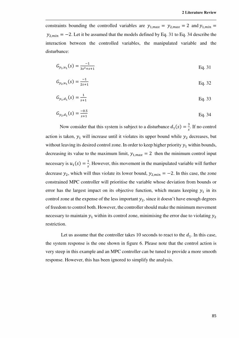
2 Literature Review
85
constraints bounding the controlled variables are w�,�?� = w�,�?� = 2 andw�,�'* =w�,�'* = −2. Let it be assumed that the models defined by Eq. 31 to Eq. 34 describe the
interaction between the controlled variables, the manipulated variable and the
disturbance:
�Q�,P�k^m = .�W�p|�|� Eq. 31
�Qp,P�k^m = .���|� Eq. 32
�Q�,,�k^m = ��|� Eq. 33
�Qp,,�k^m = .B.��|� Eq. 34
Now consider that this system is subject to a disturbanceë�k^m = W�. If no control
action is taken, w� will increase until it violates its upper bound while w� decreases, but
without leaving its desired control zone. In order to keep higher priority w� within bounds,
decreasing its value to the maximum limit, w�,�?� = 2 then the minimum control input
necessary isf�k^m = ��. However, this movement in the manipulated variable will further
decreasew�, which will thus violate its lower bound, w�,�'* = −2. In this case, the zone
constrained MPC controller will prioritise the variable whose deviation from bounds or
error has the largest impact on its objective function, which means keeping w� in its
control zone at the expense of the less important w�, since it doesn’t have enough degrees
of freedom to control both. However, the controller should make the minimum movement
necessary to maintain w� within its control zone, minimising the error due to violating w�
restriction.
Let us assume that the controller takes 10 seconds to react to the ë�. In this case,
the system response is the one shown in figure 6. Please note that the control action is
very steep in this example and an MPC controller can be tuned to provide a more smooth
response. However, this has been ignored to simplify the analysis.
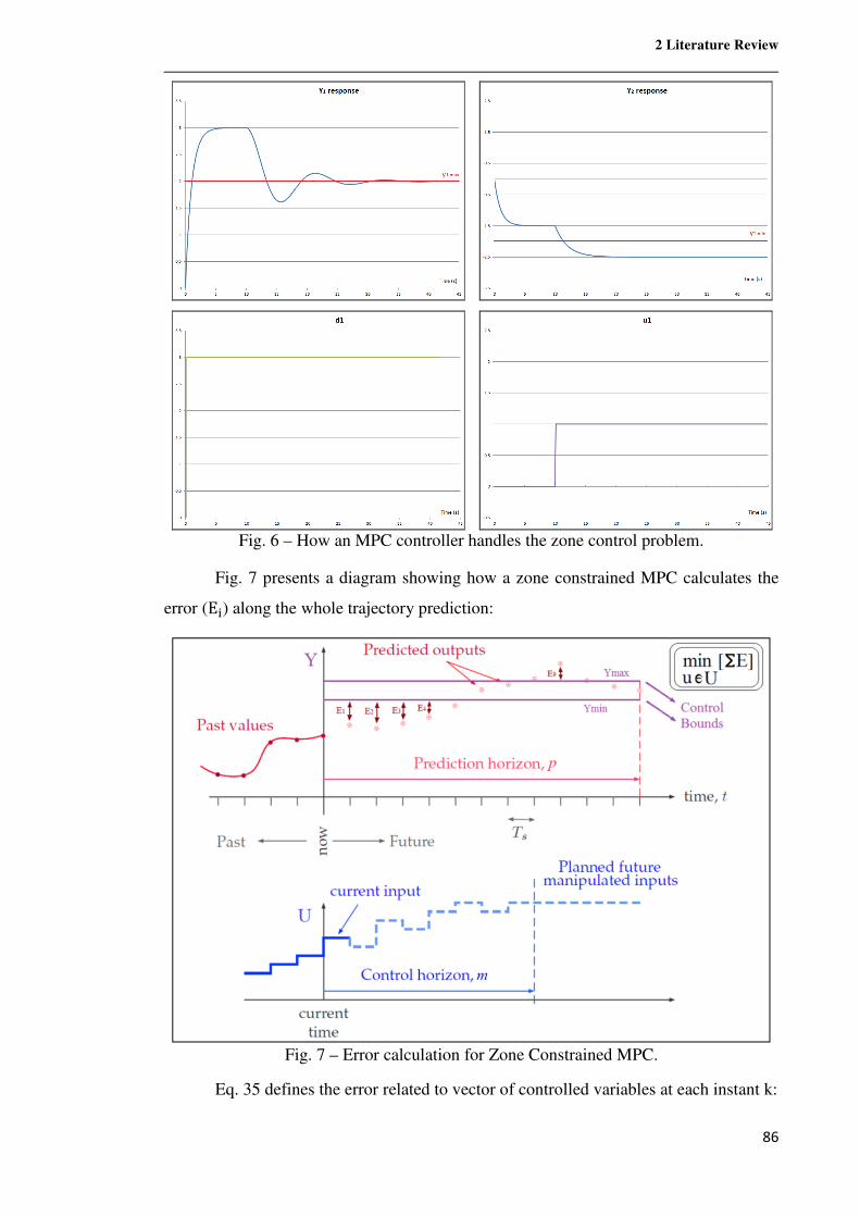
2 Literature Review
86
Fig. 6 – How an MPC controller handles the zone control problem.
Fig. 7 presents a diagram showing how a zone constrained MPC calculates the
error (E¬) along the whole trajectory prediction:
Fig. 7 – Error calculation for Zone Constrained MPC.
Eq. 35 defines the error related to vector of controlled variables at each instant k:
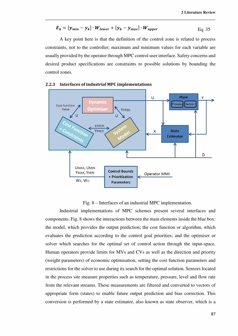
2 Literature Review
87
c\ = µ��Vh − �\· ∙ s�de�T + µ�\ − ���· ∙ s�YY�T Eq. 35
A key point here is that the definition of the control zone is related to process
constraints, not to the controller; maximum and minimum values for each variable are
usually provided by the operator through MPC control user interface. Safety concerns and
desired product specifications are constraints to possible solutions by bounding the
control zones.
2.2.3 Interfaces of industrial MPC implementations
Fig. 8 – Interfaces of an industrial MPC implementation.
Industrial implementations of MPC schemes present several interfaces and
components. Fig. 8 shows the interactions between the main elements inside the blue box:
the model, which provides the output prediction; the cost function or algorithm, which
evaluates the prediction according to the control goal priorities; and the optimiser or
solver which searches for the optimal set of control action through the input-space.
Human operators provide limits for MVs and CVs as well as the direction and priority
(weight parameters) of economic optimisation, setting the cost function parameters and
restrictions for the solver to use during its search for the optimal solution. Sensors located
in the process site measure properties such as temperature, pressure, level and flow rate
from the relevant streams. These measurements are filtered and converted to vectors of
appropriate form (states) to enable future output prediction and bias correction. This
conversion is performed by a state estimator, also known as state observer, which is a
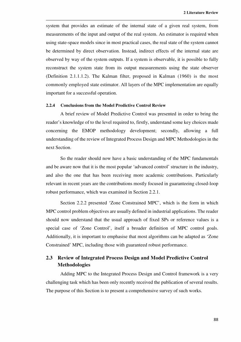
2 Literature Review
88
system that provides an estimate of the internal state of a given real system, from
measurements of the input and output of the real system. An estimator is required when
using state-space models since in most practical cases, the real state of the system cannot
be determined by direct observation. Instead, indirect effects of the internal state are
observed by way of the system outputs. If a system is observable, it is possible to fully
reconstruct the system state from its output measurements using the state observer
(Definition 2.1.1.1.2). The Kalman filter, proposed in Kalman (1960) is the most
commonly employed state estimator. All layers of the MPC implementation are equally
important for a successful operation.
2.2.4 Conclusions from the Model Predictive Control Review
A brief review of Model Predictive Control was presented in order to bring the
reader’s knowledge of to the level required to, firstly, understand some key choices made
concerning the EMOP methodology development; secondly, allowing a full
understanding of the review of Integrated Process Design and MPC Methodologies in the
next Section.
So the reader should now have a basic understanding of the MPC fundamentals
and be aware now that it is the most popular ‘advanced control’ structure in the industry,
and also the one that has been receiving more academic contributions. Particularly
relevant in recent years are the contributions mostly focused in guaranteeing closed-loop
robust performance, which was examined in Section 2.2.1.
Section 2.2.2 presented ‘Zone Constrained MPC’, which is the form in which
MPC control problem objectives are usually defined in industrial applications. The reader
should now understand that the usual approach of fixed SPs or reference values is a
special case of ‘Zone Control’, itself a broader definition of MPC control goals.
Additionally, it is important to emphasise that most algorithms can be adapted as ‘Zone
Constrained’ MPC, including those with guaranteed robust performance.
2.3 Review of Integrated Process Design and Model Predictive Control
Methodologies
Adding MPC to the Integrated Process Design and Control framework is a very
challenging task which has been only recently received the publication of several results.
The purpose of this Section is to present a comprehensive survey of such works.
2 Literature Review
89
2.3.1 Embedding MPC in Flowsheet Analysis
As discussed in the Literature Review of Methods of Integrated Control and
Process Synthesis, Chapter 2, there are several interesting papers where the integrated
design methodology is applied to determinate the optimal design and control structure for
a given process. Most of them undertake challenging issues in the integrated design
framework such as alternative procedures to evaluate controllability, uncertainties
handling techniques, the inclusion of different control strategies or address a complex
application. An important aspect of these works on integrated design is the type of
controllers and control strategies considered. Given how necessary and widespread
considered conventional feedback controllers such as PI or PID are for the control of
continuous processes such as those found in the chemical industry, it is only natural that
the bulk of simultaneous design and control methodologies developed for chemical
processes use this kind of control structure in their analysis, and these works were covered
in Section 2.1. The works that deal with advanced control structures, such as the hugely
popular Model Predictive Control, are yet few. All of them, to the author’s knowledge,
are discussed in this Section.
Until now, MPC schemes appear seldom in the framework’s literature because the
application of advanced control strategies in the integrated design framework is limited
by the complexity of the resulting optimisation problems. However, the availability of
improved computational resources allowing more powerful optimisation and computing
methods, together with mature Controllability Analysis tools and advanced control
technologies, provide the necessary driving force to address advanced control techniques,
which introduce significant improvements in the process dynamic performance,
particularly in the multivariable cases. MPC has become the advanced control method of
choice in the chemical industries such oil refining for mixture separation, reactors and
product blending, and for this reason, its insertion in the integrated design framework is
a desirable development.
Integrated design of the chemical processes and MPC controller problem consists
of simultaneously determining the plant and MPC controller parameters together with a
steady state working point, while the investment and operating costs are minimised.
Applied in the design stage of a plant design, the MPC control has a higher potential for
reducing the necessity for oversizing than the usual feedback controllers like the PID
controller, especially for systems with large delays, nonlinear response, and MIMO
system with considerable loop interactions.
2 Literature Review
90
Perhaps Brengel and Seider (1992) was the first work to propose advanced
strategies to extend the integrated design approach to use a nonlinear MPC control. The
nonlinear analysis was carried to obtain more economical designs that are flexible and
controllable in regimes characterised by greater sensitivities to modelling errors
(process/model mismatch) and changes in set-points, and in the rejection of disturbances
are more difficult to achieve. Through the applications of nonlinear programming for
multi-objective design, operations and control optimisation, they argue that it should be
possible to reduce the occurrence of overdesign in the process industries. The MPC
control is formulated as an NLP that includes a differential-algebraic by the state-space
model for the process. An interesting Section of this paper is the one which approaches
“coordinated optimisations”. The NLP solver uses the process model to evaluate the
design objective function as well as the controllability of the proposed design, as the
design optimisation proceeds. The idea is to simulate several disturbance scenarios and
to penalise the design objective for poor controllability, which results in decreased
profitability due to off-spec production. This was achieved by combining the two NLPs
for design and control such that the results of each one affect the other. A nonlinear
fermentation process was used as a study case and a coordinated optimisation strategy to
solve the simultaneous problem is proposed, where the economic objective function is
penalised by deficient controllability. This translates into a bi-level programming
problem (BPP) which is later on simplified to obtain a solution, which can be classified
as a multi-objective formulation (see Section 2.1.3.5). This work was published before
robust MPC became the norm is thus no attention is paid to guaranteed closed-loop
stability.
Loeblein and Perkins (1999) introduce a methodology for analysing the economic
performance of different structures of an integrated MPC and on-line optimisation
system. The tuning of non-constrained MPC and the evaluation of its performance within
the optimisation framework are performed. The variance of the constrained variables of
a closed-loop system subject to stochastic disturbances is calculated and then the
necessary amount of back-off from the constraints due to disturbance realisations is
analysed and later related to process economics. A simulated case study of a fluid-
catalytic cracker is used to illustrate the methodology, but it consisted only of the riser-
regenerator section. Monte Carlo simulations were used to confirm method predictions.
Although process simulation was available, the magnitude of model uncertainty was just
assumed. Also, no guidance was provided on how to obtain the uncertainty parameters.
2 Literature Review
91
Contributions made in recent years include Sakizlis et al. (2003) and Sakizlis et
al. (2004), which presented an extension of the process and control design framework that
incorporates parametric model-based predictive controllers. Applying parametric
programming for the controller derivation, the authors removed the need for solving an
optimisation problem online by giving rise to a closed-form controller structure.
Parametric programming algorithms derive the explicit mapping of the optimal control
actions in the space of the state measurements. Thus, a simple explicit state feedback
controller was derived that moves off-line the embedded on-line control optimisation and
preserves all the beneficial features of MPC. The solution consists of a set of affine
control functions in terms of the states and a set of regions where these functions are valid.
This mapping of the manipulated inputs in the state space constitutes a feedback
parametric control law for the system. The authors applied this strategy to a typical
Benzene/Toluene distillation column, proving significant economic and operability
benefits. The embedded MPC structure added terminal constraints to guarantee Lyapunov
closed-loop stability, which is missing in some similar works.
Baker and Swartz (2006) discussed the advantages of integrated design and the
importance of accounting for actuator saturation, which could lead to suboptimal designs.
In order to consider actuator saturation effects in the integrated design and control, which
results in model discontinuities, and to avoid potential difficulties with a sequential
solution approach in which the integration of the model differential-algebraic equation
system is separated from the optimisation, they followed a simultaneous solution
approach in which the actuator saturation is handled through mixed-integer constraints.
The authors also considered integrated design and control with constrained model
predictive control (MPC). The resulting problem shares the characteristic of model
discontinuity with the actuator saturation problem above, but is more complex, since the
control calculation involves the solution of a quadratic programming (QP) problem at
every sampling period. When embedded within a design optimisation problem, this
results in a multi-level optimisation problem. The authors proposed a simultaneous
solution approach in which the MPC optimisation subproblems are replaced by their
Karush-Kuhn-Tucker (KKT) optimality conditions. This results in a single-level
optimisation problem with complementarity constraints. An interior point algorithm
designed for mathematical programs with complementarity constraints was found to solve
the problem more reliably and significantly faster than a mixed-integer quadratic
2 Literature Review
92
programming formulation. However, it is not made clear by the authors how the
process/model mismatch could be handled using the methodology.
An approach to deal with process/model mismatch is given in Chawankul et al.
(2007). A variability cost is attributed each CV and the sum of capital and operating costs
are added into a single objective function. The MPC internal model is a nominal linear
model with parameter uncertainty, resulting in a robust model that represents the
nonlinear process by a family of linear models. This approach avoided nonlinear dynamic
simulations, offering computational advantages. The worst-case variability was
quantified and its associated economic cost was calculated and referred to as the robust
variability cost. This integrated method was applied to design a multi-component
distillation column. A downside is that this methodology uses as process model a dynamic
matrix of response coefficients. This approach is not as flexible and rigorous as state-
space models, and thus it has for long been abandoned by most of the academia
(Lundström et al., 1995; Lee, Morari and Garcia, 1994).
Francisco et al. (2011), whose methodology is intended to provide simultaneously
the plant dimensions, the control parameters and a steady state working point using an
IHMPC formulation with a terminal penalty and a model uncertainty approach for
robustness. The optimisation problem is a multi-objective nonlinear constrained
optimisation problem, including capital and operating costs and controllability indexes.
Differently, from the previous works reviewed here, the authors used an MPC formulation
which operates over an infinite horizon in order to guarantee stability. This IHMPC was
implemented with a terminal penalty and a multi-model approach for robust performance.
As it is often the case in integrated design papers, the methodology presented made use
of norm-based indexes to assess controllability. The optimisation problem is stated as a
multi-objective nonlinear constrained optimisation problem. The objective functions
include investment, operating costs and dynamical controllability indexes based on the
weighted sum of some norms of different closed-loop transfer functions of the system.
The paper illustrated the application of the proposed methodology with the design of the
activated sludge process of a wastewater treatment plant. A comparison between this
procedure and the Economic MPC Optimisation index is presented in Section 7.2.
However, performing this comparison was made somewhat difficult by the fact that
Francisco et al. (2011) presented several controllability indexes without discussing how
they should be prioritised, or how the different measures are related to each other.
2 Literature Review
93
Sánchez-Sánchez and Ricardez-Sandoval (2013a) presented a new integration of
process flowsheet and control design methodology that incorporates MPC strategy in the
robust analysis (see Section 2.1.4.2 for other robust methodologies). It consists of several
layers of optimisation problems: dynamic flexibility analysis, a robust dynamic feasibility
analysis, a nominal stability analysis, and a robust asymptotic stability analysis. The
robust dynamic feasibility test implements a norm-bounded analysis that computes the
critical realisations in the disturbances that produce the worst-case variability in the
outputs. Likewise, process asymptotic stability is enforced by adding a formal asymptotic
stability test. Those layers enable the specification of an optimal design that remains
feasible and asymptotically stable despite critical realisations in the disturbances. The
methodology incorporates structural decisions in the analysis for the selection of an
optimal process flowsheet while formulating the analysis as a convex problem for which
efficient numerical algorithms exist. The simultaneous process flowsheet and MPC
design method were tested on a system of Continuous Stirred Tank Reactors. It is worth
noting that the MPC formulation embedded in the analysis is perhaps over-simplistic
since no effort was made to ensure the stability of the closed loop. Sakizlis et al. (2004)
have a better approach in this particular case.
An updated method was presented by Bahakim and Ricardez-Sandoval (2014),
involving the identification of an internal MPC model and solving an optimisation
problem at each time step in which the MPC algorithm rejected stochastic-based worst-
case disturbances. The control performance was added to a design cost function that also
included the capital costs derived from equipment sizing parameters. The authors discuss
the idea behind most of the optimisation -based approaches for simultaneous design and
control, which is to determine the disturbances that produce the largest deviations in key
controlled variables and therefore demand significant efforts from the control system to
maintain the process within specifications in the presence of these conditions. Often
termed worst-case scenario, this strategy is used by the simultaneous design and control
methodologies to evaluate a design cost function. The several process constraints have to
be considered in the analysis as well in order to contemplate the worst-case scenario in a
safe and acceptable fashion without violating the critical operating restrictions of the
system. An issue that this approach has is the challenge presented to the user in providing
adequate parameters for the worst-variability distribution function. The assumption that
this advanced degree of process knowledge is available is quite strong.
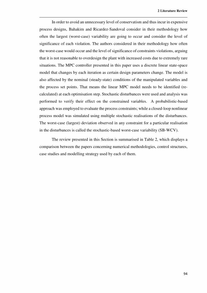
2 Literature Review
94
In order to avoid an unnecessary level of conservatism and thus incur in expensive
process designs, Bahakim and Ricardez-Sandoval consider in their methodology how
often the largest (worst-case) variability are going to occur and consider the level of
significance of each violation. The authors considered in their methodology how often
the worst-case would occur and the level of significance of constraints violations, arguing
that it is not reasonable to overdesign the plant with increased costs due to extremely rare
situations. The MPC controller presented in this paper uses a discrete linear state-space
model that changes by each iteration as certain design parameters change. The model is
also affected by the nominal (steady-state) conditions of the manipulated variables and
the process set points. That means the linear MPC model needs to be identified (re-
calculated) at each optimisation step. Stochastic disturbances were used and analysis was
performed to verify their effect on the constrained variables. A probabilistic-based
approach was employed to evaluate the process constraints; while a closed-loop nonlinear
process model was simulated using multiple stochastic realisations of the disturbances.
The worst-case (largest) deviation observed in any constraint for a particular realisation
in the disturbances is called the stochastic-based worst-case variability (SB-WCV).
The review presented in this Section is summarised in Table 2, which displays a
comparison between the papers concerning numerical methodologies, control structures,
case studies and modelling strategy used by each of them.
2 Literature Review
95
Table 2 – Paper comparison of integrated process design and MPC methodologies.
Numerical
Methodology MPC
Structure Case Study
Process
Case Study Scale /
Complexity Model
Brengel and Seider (1992)
NLP (omotopy-
continuation method)
Nonlinear Economic
Fermentation
Plant Small/Low Phenomelological
Loeblein and Perkins (1999)
Quadratic programming
(QP)
Linear Unconstrained
Fluid-Catalytic Cracker
Small/Low (linear
model, 3 outputs, 2
inputs)
Hybrid Model
Sakizlis et al. (2004)
Mixed-Integer
Nonlinear Programming
(MINLP)
Parametric Binary
Distillation Small/Low Phenomenological
Baker and Swartz (2006)
NLP (Interior Point
Algorithm) Linear CSTR Small/Low Phenomenological
Chawankul et al. (2007)
Linear Programming
(LP) Linear
Binary Distillation
Small/Low
Phenomenological/Step test
Francisco et al. (2011)
Sequential Quadratic
Programming (SQP) and
Multi-Objective
Goal Attainment
Optimisation
Infinite Horizon
Activated Sludge Process
(Wastewater Treatment)
Small/Low Phenomenological
Sanchez-Sanchez and Ricardez-Sandoval (2013)
Mixed-Integer
Nonlinear Programming (MINLP) and
Quadratic Programming
(QP)
Linear Constrained
CSTR Small/Low Phenomenological
Bahakim and Ricardez-Sandoval (2014)
Global Optimisation
(Genetic Algorithms)
Linear Wastewater
plant Small/Low Phenomenological
2.3.2 Conclusions from the review of integrated process design and MPC methodologies
MPC control has a higher potential for reducing the necessity for oversizing than
the usual feedback controllers like the PID controller, especially for systems with large
delays, nonlinear response, and MIMO system with considerable loop interactions. While
it is desirable to incorporate MPC in the simultaneous design and control methodology,
significant computational challenges that arise from the methodologies already proposed

2 Literature Review
96
with this goal, e.g., the need to identify an internal MPC model and solve an optimisation
problem (which may or not be convex) at each time step and simulating the resulting
system. This is an issue that the works reviewed in this Section could not entirely
overcome with the possible exception of Sakizlis et al. (2004), which proposes a different
approach using parametric MPC that does not require dynamic simulations.
Even without embedding MPC, finding the global solution for plantwide
optimisation can be already a challenging task as NLP and MINLP problems are
notoriously hard to solve (Sakizlis et al., 2004). Even without accounting for control
performance of the resulting flowsheet, plantwide optimisation is not commonly
employed in most projects of chemical and petrochemical plants due to the complexity of
the resulting problems and the inherent difficulty of achieving a global solution for several
thousands of nonlinear and often discontinuous equations. Hence for industrial
applications, plantwide optimisation has often been rejected in favour of sequential design
strategies. This framework consists of defining the design of each single equipment as a
segregated optimisation problem, and using one subsystem’s solution to provide next
one’s input conditions, and thus reducing the number of variables and computing time.
This approach currently works better for the large problem and will remain to do so for
the foreseeable future.
The existing framework concerning integrated process design and MPC
methodologies is subject to these same restrictions applicable to standalone plantwide
optimisation, but when MPC is embedded in the objective function, these become more
limiting. Therefore, in addition to not being effective under circumstances where
plantwide optimisation is unsuitable, the body of work covered in this Section adds
another layer of numerical and modelling complexity. As stated by Ricardez-Sandoval et
al. (2009), the algorithmic framework involving MPC is computationally demanding even
when a small number of process units are considered. Of course, it is true that the works
discussed in this Section were undoubtedly successful in addressing ideally behaved
processes such as binary distillation columns of chemically similar solvents and other
separation processes of mixtures presenting near-ideal behaviour, i.e., systems whose
deviation from Raoult's law can be ignored, or non-ideal solutions to which Raoult's law
applies and fugacity and activity coefficients can be easily calculated. For a process that
can be easily and satisfactory modelled such as these, the available integrated MPC and
design problem framework was proven to be adequate.
2 Literature Review
97
Additionally, the range of problems to which these procedures may be applied is
further restricted by the use of phenomenological models by all works reviewed here.
While very general and elegant, this kind of model is not adequate for all kinds of
processes.
For example, difficulties arise when dealing with petroleum fractions: each
subsystem usually has well over one hundred non-ideal hypothetical components; and the
severe operating conditions mean that the behaviour of gases, solutions and mixtures is
also non-ideal; multiphase flow is very common and hard to model adequately; equipment
designs are intricate. Some petroleum refining processes such as delayed coker cannot be
satisfyingly modelled phenomenologically, and in this cases, design teams use
commercial process simulators whose models rely on statistical information, e.g., neural
networks or hybrid models, which are closed-source intellectual property. That being the
case, the user is not provided with the set of equations being used. For those reasons, and
the time and engineering effort required for rigorous modelling is always very large and,
unless models are linearised, even with the optimisation solvers and processing power
available at the time of writing, it is doubtful that a solution could be found in reasonable
time. To avoid these issues, the state-space models used by the EMOP method are
obtained through the classical approach of assessing the dynamic response to step
increments in the MVs and DVs, as discussed in Chapter 3.
Another problem with the methodologies discussed here is that they always
assume that a certain MPC formulation will be used, instead of being valid for any generic
MPC algorithm. Furthermore, the control objectives were defined as SPs and not as
control zones, which are more general formulations (see Section 2.2.2 for details). Given
the usefulness and popularity of these control schemes, this is restrictive and an important
omission.
Briefly, not all process design necessities and use cases are covered by the body
of work presented in this Section. There is an important gap. Precisely the kind of process
that is hard to model and numerically demanding would benefit greatly from improved
design, which could guarantee longer operating times and greater profitability for capital-
intensive industrial operations. The EMOP method addresses this challenge.
2 Literature Review
98
2.4 The Linear Hybrid Systems framework
This Thesis presents a novel method for the linear approximation of nonlinear
systems using multiple linear models, called Simultaneous Multi-Linear Prediction
(SMLP), which is detailed in Section 4. For this reason, it is necessary to provide some
information about the state-of-art multi-model approaches that are currently available
alternatives as to the SMLP. Such approaches can be classified into the Linear Hybrid
Systems framework, presented in this Section.
A hybrid system is a collection of digital programs interacting with each other and
with an analogue environment. Each logic state of the digital part of the hybrid system
acts on the analogue part inducing a different operational mode. On the other hand, the
evolution of the analogue part triggers switches in the states of the digital part. Many
physical phenomena admit a natural hybrid description, such as control valve saturation;
digital controllers embedded in a continuous process, which act on on/off valves; process
equipment switching; switching on and off the electrical motor of pumps and
compressors, and many others complications that demand adequate modelling. Moreover,
some of the linear hybrid classes can be used to reduce the prediction error induced by
process nonlinearity, a goal that the current work shares. Christophersen (2006) defined
a general class of Linear Hybrid Systems that includes the following classes:
• Mixed logical dynamical systems;
• Linear complementary systems;
• Max-min-plus-scaling systems;
• Polyhedral piecewise affine systems or piecewise affine systems;
Bemporad and Morari (1999) introduced the mixed logical dynamical systems. In
this framework, auxiliary variables are used to transform logical facts involving
continuous variables into linear inequalities. These auxiliary variables are incorporated
into the state-space and used to update the state vector, expressing relations that describe
interdependent physical laws, logic rules, and operating constraints. Saturation functions,
discrete inputs, qualitative outputs, bilinear systems and finite state machines can be
modelled by this class, which also provides a multi-model approach by expressing
nonlinear dynamic systems through combinational logic as piecewise linear time-
invariant dynamic systems.
Another hybrid system class was introduced in the seminal paper Heemels et al.
(2000), which used ideas from the theory of the linear complementarity systems (LCS).
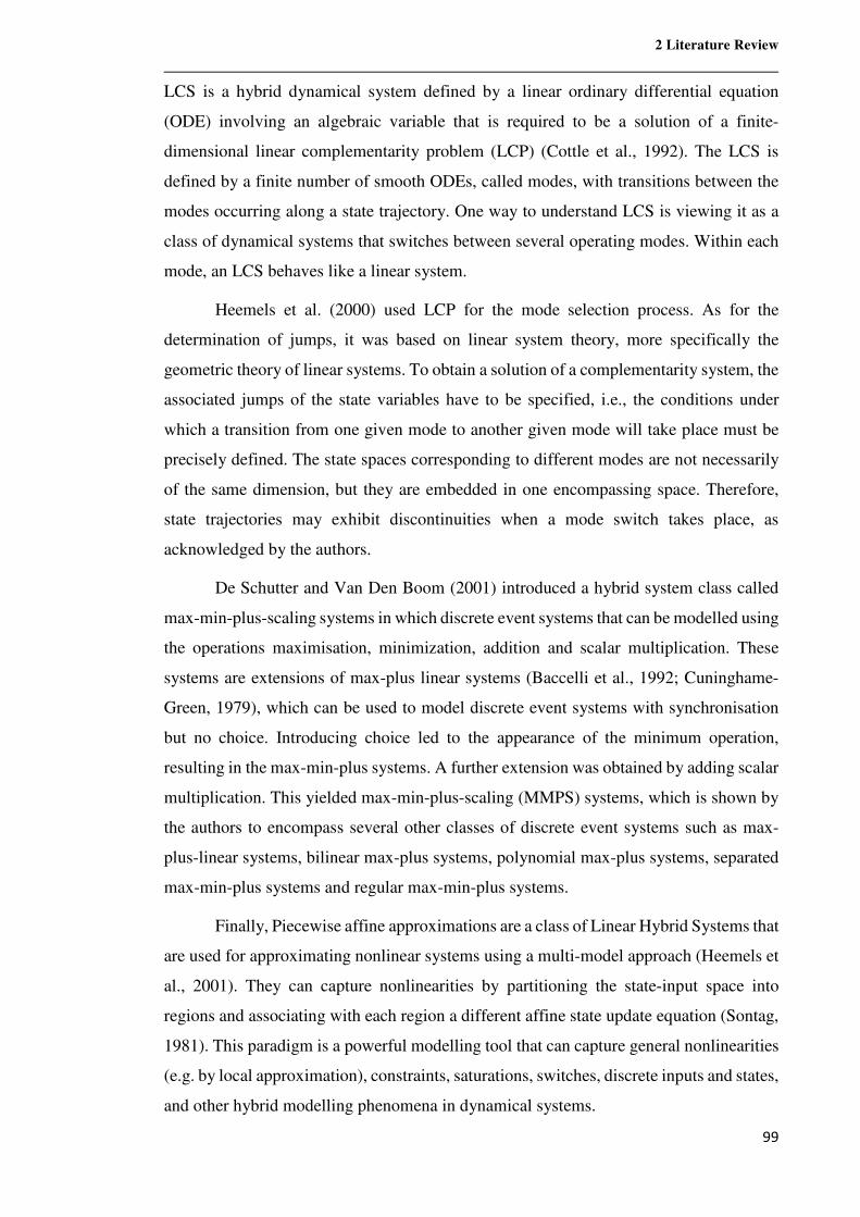
2 Literature Review
99
LCS is a hybrid dynamical system defined by a linear ordinary differential equation
(ODE) involving an algebraic variable that is required to be a solution of a finite-
dimensional linear complementarity problem (LCP) (Cottle et al., 1992). The LCS is
defined by a finite number of smooth ODEs, called modes, with transitions between the
modes occurring along a state trajectory. One way to understand LCS is viewing it as a
class of dynamical systems that switches between several operating modes. Within each
mode, an LCS behaves like a linear system.
Heemels et al. (2000) used LCP for the mode selection process. As for the
determination of jumps, it was based on linear system theory, more specifically the
geometric theory of linear systems. To obtain a solution of a complementarity system, the
associated jumps of the state variables have to be specified, i.e., the conditions under
which a transition from one given mode to another given mode will take place must be
precisely defined. The state spaces corresponding to different modes are not necessarily
of the same dimension, but they are embedded in one encompassing space. Therefore,
state trajectories may exhibit discontinuities when a mode switch takes place, as
acknowledged by the authors.
De Schutter and Van Den Boom (2001) introduced a hybrid system class called
max-min-plus-scaling systems in which discrete event systems that can be modelled using
the operations maximisation, minimization, addition and scalar multiplication. These
systems are extensions of max-plus linear systems (Baccelli et al., 1992; Cuninghame-
Green, 1979), which can be used to model discrete event systems with synchronisation
but no choice. Introducing choice led to the appearance of the minimum operation,
resulting in the max-min-plus systems. A further extension was obtained by adding scalar
multiplication. This yielded max-min-plus-scaling (MMPS) systems, which is shown by
the authors to encompass several other classes of discrete event systems such as max-
plus-linear systems, bilinear max-plus systems, polynomial max-plus systems, separated
max-min-plus systems and regular max-min-plus systems.
Finally, Piecewise affine approximations are a class of Linear Hybrid Systems that
are used for approximating nonlinear systems using a multi-model approach (Heemels et
al., 2001). They can capture nonlinearities by partitioning the state-input space into
regions and associating with each region a different affine state update equation (Sontag,
1981). This paradigm is a powerful modelling tool that can capture general nonlinearities
(e.g. by local approximation), constraints, saturations, switches, discrete inputs and states,
and other hybrid modelling phenomena in dynamical systems.
2 Literature Review
100
PWA systems can approximate nonlinear systems via multiple linearisations at
different operating points (OP) (Sontag, 1981; Ferrari-Trecate et al., 2003; Roll et al.,
2004). Space is partitioned through a series of linear approximations. As the plant
operating point moves throughout the state-input space, the state update equation is
changed according to the linear model valid locally, as shown in Fig. 9. The larger the
number of partitions the closer the approximations become to the nonlinear model.
Fig. 9 – The operating point moves through the boundaries of a PWA system.
A Literature Review of switched and PWA models is presented in Roll (2003),
and a tutorial paper in Paoletti et al. (2007). A survey on switched and piecewise affine
system identification is presented in Garulli et al. (2012), from which the main approaches
on the topic were presented. These main types of approaches were classified as
optimisation-based, algebraic and recursive methods for Switched Autoregressive
Exogenous (SARX) models, optimisation-based and clustering-based methods for
PieceWise ARX (PWARX) models, and batch and recursive methods for state-space
systems. According to Garulli et al. (2012), a common feature of the approaches, which
is present in works such as Vidal et al. (2003), Roll et al. (2004), Ferrari-Trecate et al.
(2003), Nakada et al. (2005), Juloski et al. (2005) and Bemporad et al. (2005), is that they
lead to suboptimal solutions to the problem of inferring a PWARX model from data,
while keeping an affordable computational burden.
In Section 4 a few shortcomings of PWA systems while used to represent model
nonlinearity are discussed. These shortcomings motivated the development of the SMLP
method, and in that Section it is discussed how it addressed them.
Changes in the state
update equation
StateX
Partition boundaries M�
M�
MW
Mv
M�
2 Literature Review
101
2.5 Conclusions from the Literature Review
Considering the discussion presented in this Chapter, it becomes clear that the
most obvious gap in the existing Integrated Control and Process Synthesis (ICPS) body
of work is the lack of an MPC-embedded method suitable for large-scale plants. This is
in part caused by the increased complexity of the MPC control problem as compared to
relatively simple feedback control structures, resulting in numerical and modelling
challenges. Another issue is that while feedback controllers consist mostly in standardised
PIDs, hundreds of distinct MPC algorithms exist, and each of the ICPS methods with
embedded MPC discussed in Section 2.3 uses a different algorithm in their cost functions
and simulations. Since the closed loop behaviour is being considered, the conclusions
obtained by these methods are not valid for other algorithms, and even for different
selections of tuning parameters. Furthermore, the closed loop analysis results in an
optimisation problem composed of several layers that can be rapidly become intractable
for larger systems, which are the main subjects of this work. Another gap currently found
in the ICPS framework is the lack of a method with control goals defined as zones.
Therefore, it is desirable to devise a methodology capable of fillings these gaps while
tackling the challenge of a high computational demand. With this in mind, the Economic
MPC Optimisation index is introduced in the next Chapter.
3 Assessing Plant Design for MPC Performance
102
3 Assessing Plant Design for MPC Performance
The starting point of the Economic MPC Optimisation index methodology is a set
of previously generated candidate designs, which are kept fixed during the analysis. Since
the approach adopted is sequential, one could classify the EMOP methodology as part of
the Controllability Analysis framework (Sections 2.1.1 and 2.1.2) rather than ICPS
(Section 2.1.3). At the same time, the sequential approach opens an interesting possibility:
using the EMOP index in addition to any ICPS procedure in order to test and validate the
flowsheets generated (as done in Section 7.2 for the activated sludge process). Another
relevant choice made during the design of the EMOP methodology was to deal only with
open loop dynamic behaviour and make no assumptions towards closed-loop
performance since these cannot be generalised across different MPC algorithms. The
main drawback of dealing solely with the open-loop is the need of all plants to be
bounded-input, bounded-output stable while closed-loop methods can design plants with
less rigorous degrees of stability.
For the goal of embedding MPC in the IPDCF while dealing with large-scale,
complex systems, segregating the problems of optimising capital expenditures (CAPEX)
and operating expenses (OPEX) was the sensible choice. Restricting the analysis to
OPEX greatly simplifies modelling and simulation and avoids the use of decision
variables and the need for mixed-integer programming. This is the first reason why the
candidate flowsheets were fixed; the second reason is to enable the use of commercial
simulation packages to provide the models instead of first-principle models for most
usage scenarios. The EMOP index makes use of multiple linear state-space models
obtained through step-test model identification, a classic approach, using identification
data provided by any given dynamic simulator. Although first-principle models can be
used for simple processes, model identification is recommended for complex systems
instead of iteratively solving mass and energy balances for each cost function evaluation.
Using both a sequential approach and step response models greatly reduces the
numerical complexity of the resulting problem, enabling the analysis of larger systems
than similar methodologies. Even if the models thus obtained are linear, the effect of
process nonlinearity in the analysis can be mitigated by the use of multiples models
(Chapter 4) and by bounding results according to model uncertainty (Chapter 5).
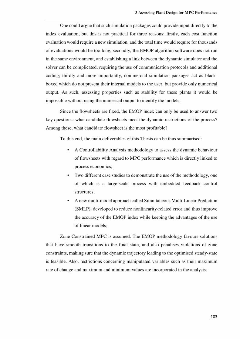
3 Assessing Plant Design for MPC Performance
103
One could argue that such simulation packages could provide input directly to the
index evaluation, but this is not practical for three reasons: firstly, each cost function
evaluation would require a new simulation, and the total time would require for thousands
of evaluations would be too long; secondly, the EMOP algorithm software does not run
in the same environment, and establishing a link between the dynamic simulator and the
solver can be complicated, requiring the use of communication protocols and additional
coding; thirdly and more importantly, commercial simulation packages act as black-
boxed which do not present their internal models to the user, but provide only numerical
output. As such, assessing properties such as stability for these plants it would be
impossible without using the numerical output to identify the models.
Since the flowsheets are fixed, the EMOP index can only be used to answer two
key questions: what candidate flowsheets meet the dynamic restrictions of the process?
Among these, what candidate flowsheet is the most profitable?
To this end, the main deliverables of this Thesis can be thus summarised:
• A Controllability Analysis methodology to assess the dynamic behaviour
of flowsheets with regard to MPC performance which is directly linked to
process economics;
• Two different case studies to demonstrate the use of the methodology, one
of which is a large-scale process with embedded feedback control
structures;
• A new multi-model approach called Simultaneous Multi-Linear Prediction
(SMLP), developed to reduce nonlinearity-related error and thus improve
the accuracy of the EMOP index while keeping the advantages of the use
of linear models;
Zone Constrained MPC is assumed. The EMOP methodology favours solutions
that have smooth transitions to the final state, and also penalises violations of zone
constraints, making sure that the dynamic trajectory leading to the optimised steady-state
is feasible. Also, restrictions concerning manipulated variables such as their maximum
rate of change and maximum and minimum values are incorporated in the analysis.
3 Assessing Plant Design for MPC Performance
104
Fig. 10 provides a workflow showing the order by which the methodologies
presented in this Thesis should be performed, including the EMOP index and SMLP
modelling.
Fig. 10 – Workflow of the joint use of the EMOP index and the SMLP.
Dynamic
Simulation
Flowsheet
Design
Generation
Simulation
Numeric Output
Step Response
Model
Identification
Generation
of the SMLP
Systems
Stability
Check
Economic Analysis
to Obtain Cost
Function Parameters
EMOP Index
Tuning (MV
restrictions)
Simulation of
Scenarios (initial
state, DV profiles,
restrictions)
Running Solver
/ Output
Prediction
EMOP Index Value
for each Scenario
and Flowsheet
EMOP Index
Ranking of
Flowsheets
1 2 3
456
7 8 9
101112
• Production targets/market conditions;
• Alternative process routes;
• Alternative process equipment technologies;
• Alternative control and instrumentation systems.
3 Assessing Plant Design for MPC Performance
105
Now each step shown in Fig. 10 is discussed in detail. The whole of these
procedures compose the EMOP index method which is one of the main deliverables of
this Thesis.
Preliminary research
Preliminary research normally includes research of market conditions and the
definition of the product being marketed; product prices and production targets; research
of alternative process routes, equipment technologies; energy and raw materials costs; but
seldom involves alternatives for control systems and instrumentation. This a standard
procedure in process engineering.
Step 1 – Flowsheet Design Generation
In this step, the candidate flowsheets are defined based on the findings of the
preliminary research. It is assumed that operation is continuous for all plants and that
control zones will be defined for each plant.
At this point, the design team has usually picked out one of the alternative process
routes and has some idea of the layout to be chosen. Differences between flowsheets
might be subtle, such as different embedded regulatory control loop structures, or they
might be moderate, e.g., different equipment layout, sizing and specifications for
operating conditions. However, it is possible the information yielded by preliminary
research was not enough to decide upon a single process route. In this case, considerable
differences among flowsheets may arise, with production routes and layouts altogether
different. In this case, the reader should consult Section 3.9.
Step 2 – Dynamic Simulation or Rigorous Modelling
Dynamic simulations of all flowsheets defined in Step 1 may be carried out in a
commercial simulation package such as Petro-Sim®, UniSim®, Hysys®, etc. As
previously discussed in this Chapter, these state-of-the-art simulators will support our
integrated design and control approach, which is intended for large-scale, complex
processes for which the full set of equations is unavailable. However, nothing prevents a
first principles model to be used if the process is relatively simple. The dynamic
simulations or first-principles model shall be referred in this Thesis as the nonlinear
model.
3 Assessing Plant Design for MPC Performance
106
Step 3 – Simulation Numeric Output (Optional)
If dynamic simulation was used, attention must be paid to the consistency of the
data generated. Its numeric output must be validated through a sufficiently broad range
of operating conditions. Output and input data must be stored in convenient data formats
such as .csv or .xlsx to be handled in the software environment containing the
optimisation solver, e.g., MATLAB®, GAMS®, etc. In this Thesis, the simulation data
is presented as a series of linear transfer functions in the Laplace domain describing the
relation between each CV, MV and DV, since this format is compact and convenient.
Step 4 – Step Response Model Identification (Optional)
Linearising the nonlinear model brings advantages when using optimisation
solvers to find the optimal operating point, resulting always in convex problems for which
fast conversion can be obtained. In this Thesis, each linearisation or approximation of the
nonlinear model is called a sub-model.
Each sub-model is to be obtained through model identification on a set of data
generated by step increments on MVs and DVs. Alternatively, the relay response could
be used. Tests may be performed on a dynamic simulator or on an experimental pilot
plant, or even on a real industrial unit, for the sake of the methodology, it is indifferent.
Let us refer to the data thus obtained as the nonlinear model data, from which the sub-
models are derived and validated. The initial state from which a test is performed will be
referred as an identification point (IP) or epicentre, and it will be considered the epicentre
of the resulting sub-model. For each input/output couple of the MIMO system, different
values for the sub-model’s order should be tested, and the order adopted is the one that
minimises the residue between the nonlinear model data and the sub-model being
considered. This procedure avoids model overfitting or underfitting, both of which can
have catastrophic results especially when the operating point (OP) is removed from the
vicinity of the model’s epicentre. In this Thesis, the identification data used was different
from the validation data, and we consider this to be a good practice.
3 Assessing Plant Design for MPC Performance
107
Step 5 – Generation of the SMLP Systems (Optional)
This step is optional as the user may also use the nonlinear model, a single linear
model or any other multi-model approach to predict plant behaviour.
The SMLP is a method for obtaining a prediction for the future values of an output
vector. Three main elements are used to provide this prediction: the initial state, the input
profiles and the set of sub-models (linear approximations of a nonlinear model) identified
at distinct states, yielded by Step 4. Hence the SMLP consists of the representation of a
flowsheet as a collection of linear state-space models, which are combined to yield an
overall output prediction.
The greater the number of sub-models, the better the resilience of the resulting
SMLP system with regard to process nonlinearity. The location of the epicentres of the
sub-models is key to the SMLP method. The control engineer should select epicentres
that are representative of the most common or critical operating conditions. In similar
fashion to the sub-model validation of Step 4, the SMLP system should be validated
against a test data set. Described in detail in Chapter 4 of this Thesis, the SMLP method
has 3 variants. These variants present a trade-off between the accuracy displayed while
emulating the nonlinear model and the time and effort required to assemble the system.
Step 6 – Stability Check
Being an open-loop reachability problem, the EMOP index only makes sense for
Bounded-Input Bounded-Output (BIBO) stable flowsheets. We are interested in the
optimal steady-state which is unbiased by the upper layer (MPC) control scheme. This
optimal OP cannot be obtained for unbounded responses. The classical stability criteria
for MIMO systems is detailed by Lyapunov (1892) (see Section 2.1.3.2). If an SMLP
system is being used, the reader is encouraged to perform the stability check presented in
Section 4.1.6.
Step 7 – Economic Analysis to Obtain Cost Function Parameters
This step provides the link between process economics and dynamics by
evaluating the impact of plant dynamic behaviour and disturbances on revenue and
OPEX. Basically, each variable receives a price tag based on product prices, quality, and
costs. This step is discussed in Sections 3.3, 3.4, 3.7 and 3.9 as the cost function is
constructed step by step. While there is no universal approach to perform this Step, since
it depends on the process and control goals considered, the main case study of this Thesis
which is shown in Chapter 6 can serve as a guideline.
3 Assessing Plant Design for MPC Performance
108
Step 8 – EMOP Index Tuning (MV restrictions)
The EMOP index is an open-loop analysis intended to find each’s flowsheet
optimal OP. There is, of course, a transient between the initial state and the optimal OP
and, just like an MPC, the OP is reached by manipulating process inputs. However, the
optimisation problem is reduced by the lack of feedback. In MPC the prediction horizon
keeps being shifted forward and for this reason, MPC is sometimes called receding
horizon control. The EMOP uses a fixed horizon instead of a receding horizon. Since no
measurement noise and no unmeasured disturbances are present, states can be calculated
from the state-space model (Section 3.1 and Appendix) without the need of using state
estimators.
There is, however, the need to ensure a smooth transition and no bound violation
between initial and optimal OPs, and this subject is covered in Sections 3.5, 3.6 and 3.8.
The control bounds on MVs usually reflect safety concerns. They may be related to
equipment restrictions such as the maximum pressure and temperature tolerated by
vessels, the minimum flow rate and the maximum head of pumps and compressors, etc.
They may also refer to limits on feed, reflux or output flow rates.
Step 9 – Simulation of Scenarios (initial state, DV profiles, restrictions)
Process knowledge is paramount for the correct implementation of the EMOP
method. This knowledge ideally encompasses the most commonly encountered
disturbances encountered for the flowsheets being assessed, e.g., changing feed
composition and production targets, changes in operating conditions such as variate
bounds in temperature, pressure, product quality, etc. These scenarios consist of a range
of operating conditions that reflect situations that are either very commonly experienced
or uncommon but critical.
Step 10 – Running Solver / Output Prediction
Based on the scenarios defined in Step 9, the solver searches for the series of
control actions leading to the OP of minimal OPEX/maximum revenue. Ideally, the same
scenarios are evaluated for every flowsheet, i.e., the same changes in operating conditions
are going to happen to all flowsheets. If this is unpractical due to existing differences in
the flowsheets, the reader should use the method described in section 3.9.
While the SMLP system is linear, nonlinear restrictions and variate parameters
introduce nonlinearities into the optimisation problem. The solver to be used must be able
to handle such complications. For the case studies presented in this Thesis, we found out
3 Assessing Plant Design for MPC Performance
109
that the Interior-Point Algorithm with Analytic Hessian provided by MATLAB® 2016b
(fmincon) was able to yield the desired results.
Step 11 – EMOP Index Value for each Scenario and Flowsheet
The gap between the EMOP indexes evaluated at the final and initial OPs yields
a monetised measure of Controllability based on dynamic behaviour differences between
flowsheets. This value is closely related to expected differences in OPEX between plants.
The basic mathematical formula for the EMOP index evaluation is provided in Section
3.4. The version incorporating smoothness concerns is presented in Section 3.5, and the
version with variate product prices is given in Section 3.7.
Step 12 – EMOP Index Ranking of Flowsheets
The indexes yielded by each scenario must be combined into a single index that
describes the overall quality of dynamic response for a certain flowsheet. A weighted
geometric average is suggested. The ranking of overall EMOP indexes shows the most
favourable among the set of candidate flowsheets.
3.1 A State-Space Methodology
Most MPC schemes make use of linear state-space models, which can be
identified with relative ease through step tests of the manipulated inputs. The prediction
yielded by space-state models can also be used to evaluate the EMOP index of a
flowsheet. Lee et al. (1994) proposed a generic linear state-space model representation in
the incremental form as defined in Eq. 36 and Eq. 37:
�\ = �\ Eq. 36
\|� = �\ + �∆�\ + �∆�\ Eq. 37
where � ∈ ℝ*� is the vector of process outputs, ∈ ℝ*� is the state vector, � ∈ℝ*� is the control input vector, � ∈ ℝ*� is the disturbance vector and ∆�\ and ∆�\ are
the matrices of MVs and DVs increments defined respectively by Eq. 38 and Eq. 39:
3 Assessing Plant Design for MPC Performance
110
∆�\ = �\|� − �\�\| − �\|�⋮�\|� − �\|�.�
" Eq. 38
∆�\ = �\|� − �\�\| − �\|�⋮�\|Y − �\|Y.�
" Eq. 39
where � is the prediction horizon and � is the number of time increments of the
control horizon, which is also the number of control actions performed. Here we assume
that the number of DV movements is equal to the prediction horizon.
The model formulation defined by Eq. 36 and Eq. 37 makes use of deviation
variables and represents a process flowsheet that is assumed to be fixed during the
analysis (this approach does not aim to replace early stage process synthesis usually based
on steady-state information). Any steady state corresponds to a point where ∆�\ = ¾ and
there is no need to know the explicit value of � at the steady state corresponding to a
particular output SP. The matrices of the linear state-space model can be identified with
relative ease through step tests of the manipulated inputs. Obtaining models from the
analytical step response is a model identification procedure that has been widely used in
the MPC framework as an option to phenomenological modelling.
This state-space representation may be applied to time delayed stable, unstable
and integrating systems as long as matrices�, �, � and can be defined to properly
represent these complications. The state-space model formulation as proposed in Strutzel
et al. (2013) meets these needs and for this reason was selected for use in this work. More
details and further developments about this kind of model representation, designated
output prediction oriented model (OPOM), which was first proposed by Rodrigues and
Odloak (2000), can be found in Martins et al. (2013), in Santoro and Odloak (2012) and
González et al. (2007).
Based on this model, we set the goal of obtaining a method to assess how
promising a given flowsheet is with regard to zone constrained MPC performance, i.e., a
method to assess which plant is better placed to accommodate DVs (Disturbance
Variables) while being optimised by an MPC. To this end, obtaining the output vector at
the end of the prediction horizon k�m is going to be useful in later Sections. At an arbitrary
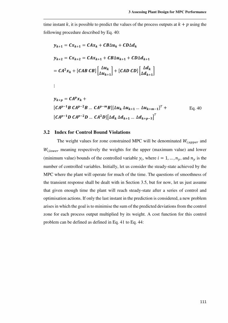
3 Assessing Plant Design for MPC Performance
111
time instant �, it is possible to predict the values of the process outputs at � + � using the
following procedure described by Eq. 40:
�\|� = �\|� = ��\ + ��∆�\ + � ∆�\
�\| = �\| = ��\|� + ��∆�\|� + � ∆�\|�
= �� \ + µ�����· # ∆�\∆�\|�$+ µ�� � · # ∆�\∆�\|�$
⋮
�\|Y = ��Y\ +µ��Y.����Y. �… ��Y.��·µ∆�\∆�\|�…∆�\|�.�·% +µ��Y.� ��Y. … �� ·&∆�\∆�\|�…∆�\|Y.'(%
Eq. 40
3.2 Index for Control Bound Violations
The weight values for zone constrained MPC will be denominated �',PNNLH and �',)K�LH meaning respectively the weights for the upper (maximum value) and lower
(minimum value) bounds of the controlled variable w', where ¹ = 1,… , MQ, and MQ is the
number of controlled variables. Initially, let us consider the steady-state achieved by the
MPC where the plant will operate for much of the time. The questions of smoothness of
the transient response shall be dealt with in Section 3.5, but for now, let us just assume
that given enough time the plant will reach steady-state after a series of control and
optimisation actions. If only the last instant in the prediction is considered, a new problem
arises in which the goal is to minimise the sum of the predicted deviations from the control
zone for each process output multiplied by its weight. A cost function for this control
problem can be defined as defined in Eq. 41 to Eq. 44:
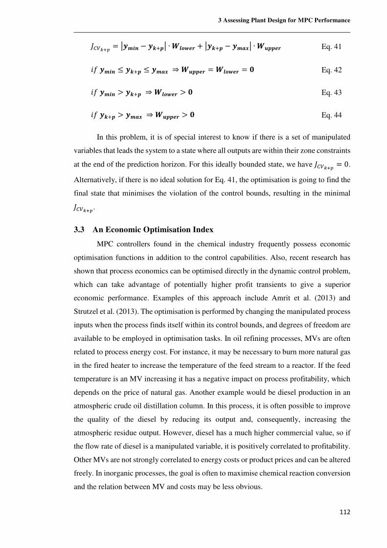
3 Assessing Plant Design for MPC Performance
112
;<=)*+ = Ø��Vh − �\|YØ ∙ s�de�T + Ø�\|Y − ���Ø ∙ s�YY�T Eq. 41
¹+��Vh ≤ �\|Y ≤ ��� ⇒s�YY�T = s�de�T = ¾ Eq. 42
¹+��Vh > �\|Y ⇒s�de�T > ¾ Eq. 43
¹+�\|Y > ��� ⇒s�YY�T > ¾ Eq. 44
In this problem, it is of special interest to know if there is a set of manipulated
variables that leads the system to a state where all outputs are within their zone constraints
at the end of the prediction horizon. For this ideally bounded state, we have ;<=)*+ = 0.
Alternatively, if there is no ideal solution for Eq. 41, the optimisation is going to find the
final state that minimises the violation of the control bounds, resulting in the minimal
;<=)*+.
3.3 An Economic Optimisation Index
MPC controllers found in the chemical industry frequently possess economic
optimisation functions in addition to the control capabilities. Also, recent research has
shown that process economics can be optimised directly in the dynamic control problem,
which can take advantage of potentially higher profit transients to give a superior
economic performance. Examples of this approach include Amrit et al. (2013) and
Strutzel et al. (2013). The optimisation is performed by changing the manipulated process
inputs when the process finds itself within its control bounds, and degrees of freedom are
available to be employed in optimisation tasks. In oil refining processes, MVs are often
related to process energy cost. For instance, it may be necessary to burn more natural gas
in the fired heater to increase the temperature of the feed stream to a reactor. If the feed
temperature is an MV increasing it has a negative impact on process profitability, which
depends on the price of natural gas. Another example would be diesel production in an
atmospheric crude oil distillation column. In this process, it is often possible to improve
the quality of the diesel by reducing its output and, consequently, increasing the
atmospheric residue output. However, diesel has a much higher commercial value, so if
the flow rate of diesel is a manipulated variable, it is positively correlated to profitability.
Other MVs are not strongly correlated to energy costs or product prices and can be altered
freely. In inorganic processes, the goal is often to maximise chemical reaction conversion
and the relation between MV and costs may be less obvious.
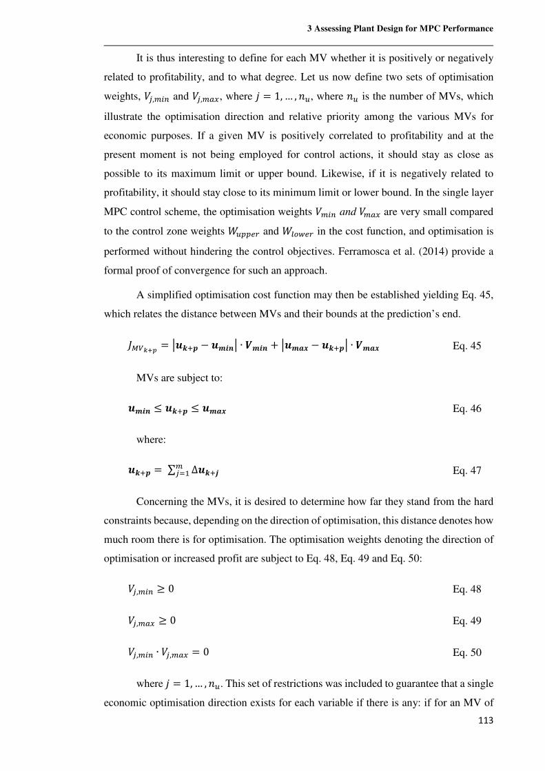
3 Assessing Plant Design for MPC Performance
113
It is thus interesting to define for each MV whether it is positively or negatively
related to profitability, and to what degree. Let us now define two sets of optimisation
weights, -Ý,�'* and -Ý,�?�, where à = 1, … , MP, where MP is the number of MVs, which
illustrate the optimisation direction and relative priority among the various MVs for
economic purposes. If a given MV is positively correlated to profitability and at the
present moment is not being employed for control actions, it should stay as close as
possible to its maximum limit or upper bound. Likewise, if it is negatively related to
profitability, it should stay close to its minimum limit or lower bound. In the single layer
MPC control scheme, the optimisation weights -�'* and -�?� are very small compared
to the control zone weights �PNNLH and �)K�LH in the cost function, and optimisation is
performed without hindering the control objectives. Ferramosca et al. (2014) provide a
formal proof of convergence for such an approach.
A simplified optimisation cost function may then be established yielding Eq. 45,
which relates the distance between MVs and their bounds at the prediction’s end.
;4=)*+ = Ø�\|Y − ��VhØ ∙ j�Vh + Ø��� − �\|YØ ∙ j�� Eq. 45
MVs are subject to:
��Vh ≤ �\|Y ≤ ��� Eq. 46
where:
�\|Y =∑ ∆�\|Õ�Ý/� Eq. 47
Concerning the MVs, it is desired to determine how far they stand from the hard
constraints because, depending on the direction of optimisation, this distance denotes how
much room there is for optimisation. The optimisation weights denoting the direction of
optimisation or increased profit are subject to Eq. 48, Eq. 49 and Eq. 50:
-Ý,�'* ≥ 0 Eq. 48
-Ý,�?� ≥ 0 Eq. 49
-Ý,�'* ∙ -Ý,�?� = 0 Eq. 50
where à = 1,… , MP. This set of restrictions was included to guarantee that a single
economic optimisation direction exists for each variable if there is any: if for an MV of
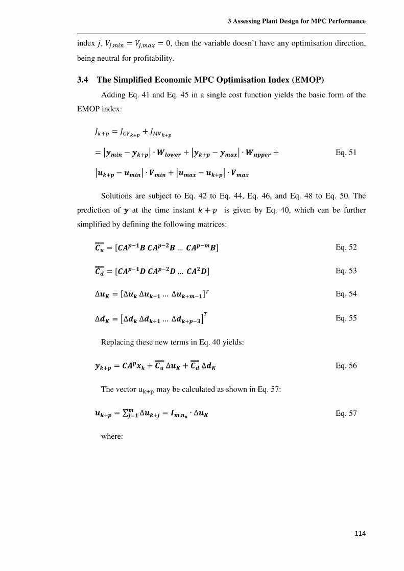
3 Assessing Plant Design for MPC Performance
114
index à, -Ý,�'* = -Ý,�?� = 0, then the variable doesn’t have any optimisation direction,
being neutral for profitability.
3.4 The Simplified Economic MPC Optimisation Index (EMOP)
Adding Eq. 41 and Eq. 45 in a single cost function yields the basic form of the
EMOP index:
;(|N = ;<=)*+ + ;4=)*+
= Ø��Vh − �\|YØ ∙ s�de�T + Ø�\|Y − ���Ø ∙ s�YY�T +
Ø�\|Y − ��VhØ ∙ j�Vh + Ø��� − �\|YØ ∙ j��
Eq. 51
Solutions are subject to Eq. 42 to Eq. 44, Eq. 46, and Eq. 48 to Eq. 50. The
prediction of � at the time instant � + � is given by Eq. 40, which can be further
simplified by defining the following matrices:
������ = µ��Y.����Y. �… ��Y.��· Eq. 52
������ = µ��Y.� ��Y. … �� · Eq. 53
∆�! = µ∆�\∆�\|�…∆�\|�.�·% Eq. 54
∆�! = &∆�\∆�\|�…∆�\|Y.'(% Eq. 55
Replacing these new terms in Eq. 40 yields:
�\|Y = ��Y\ + ������∆�! + ������∆�! Eq. 56
The vector u1|2 may be calculated as shown in Eq. 57:
�\|Y = ∑ ∆�\|Õ = ��.h� ∙ ∆�!�Õ/� Eq. 57
where:
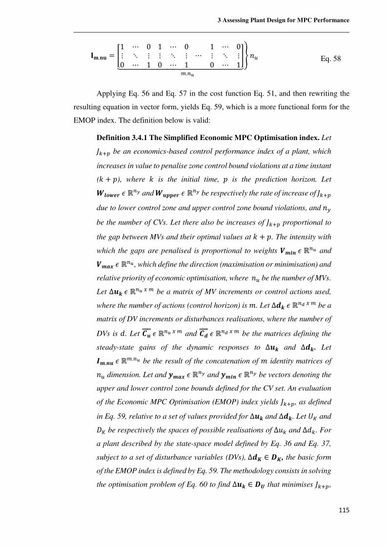
3 Assessing Plant Design for MPC Performance
115
34.56 = 71 ⋯ 0⋮ ⋱ ⋮0 ⋯ 1
1 ⋯ 0⋮ ⋱ ⋮0 ⋯ 1
⋯ 1 ⋯ 0⋮ ⋱ ⋮0 ⋯ 1
:ÇÈÈÈÈÈÈÈÈÈÈÈÉÈÈÈÈÈÈÈÈÈÈÈÊ
;MP�.*�
Eq. 58
Applying Eq. 56 and Eq. 57 in the cost function Eq. 51, and then rewriting the
resulting equation in vector form, yields Eq. 59, which is a more functional form for the
EMOP index. The definition below is valid:
Definition 3.4.1 The Simplified Economic MPC Optimisation index. Let
;(|N be an economics-based control performance index of a plant, which
increases in value to penalise zone control bound violations at a time instant
(� + �), where � is the initial time, � is the prediction horizon. Let
s�de�T<ℝ*� and s�YY�T<ℝ*� be respectively the rate of increase of ;(|N
due to lower control zone and upper control zone bound violations, and MQ
be the number of CVs. Let there also be increases of ;(|N proportional to
the gap between MVs and their optimal values at � + �. The intensity with
which the gaps are penalised is proportional to weights j�Vh<ℝ*� and
j��<ℝ*�, which define the direction (maximisation or minimisation) and
relative priority of economic optimisation, where MP be the number of MVs.
Let ∆�\<ℝ*��� be a matrix of MV increments or control actions used,
where the number of actions (control horizon) is �. Let ∆�\<ℝ*��� be a
matrix of DV increments or disturbances realisations, where the number of
DVs is ë. Let ������<ℝ*��� and ������<ℝ*��� be the matrices defining the
steady-state gains of the dynamic responses to ∆�\ and ∆�\. Let
��.h�<ℝ�.*� be the result of the concatenation of � identity matrices of
MP dimension. Let and ���<ℝ*� and ��Vh<ℝ*� be vectors denoting the
upper and lower control zone bounds defined for the CV set. An evaluation
of the Economic MPC Optimisation (EMOP) index yields ;(|N, as defined
in Eq. 59, relative to a set of values provided for ∆�\ and ∆�\. Let �= and �= be respectively the spaces of possible realisations of ∆f( and ∆ë(. For
a plant described by the state-space model defined by Eq. 36 and Eq. 37,
subject to a set of disturbance variables (DVs),∆�! ∈ !, the basic form
of the EMOP index is defined by Eq. 59. The methodology consists in solving
the optimisation problem of Eq. 60 to find ∆�\ ∈ g that minimises ;(|N,
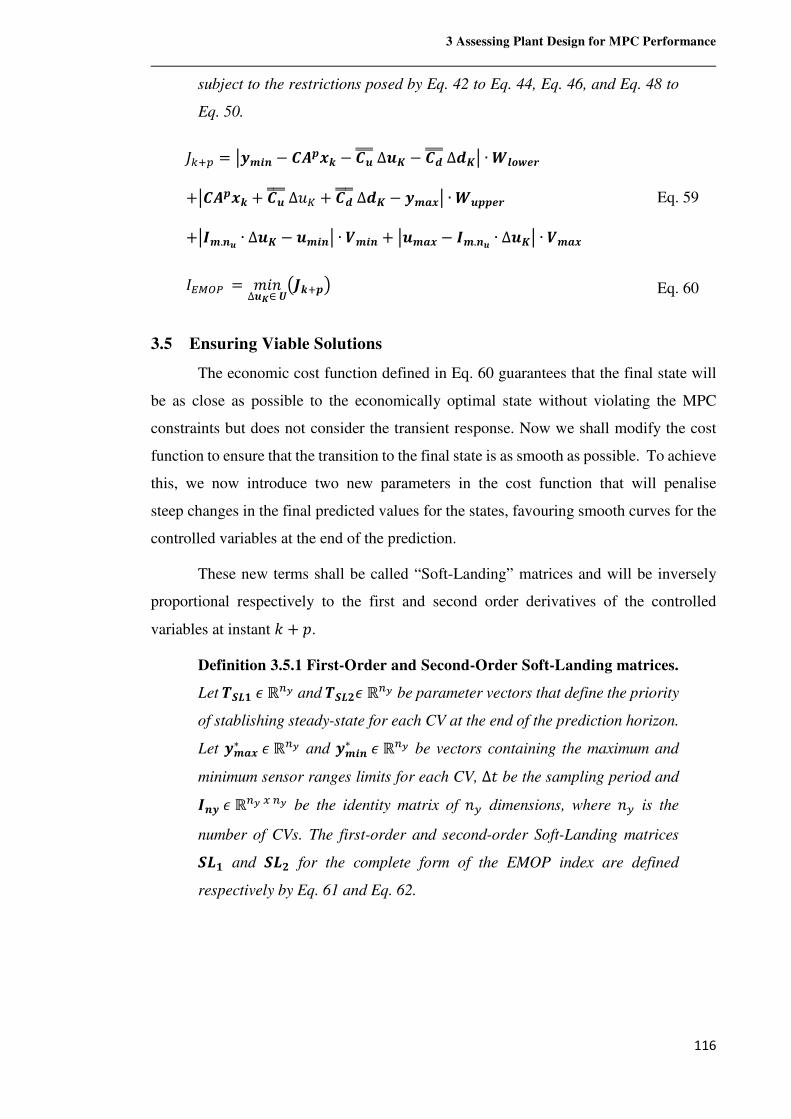
3 Assessing Plant Design for MPC Performance
116
subject to the restrictions posed by Eq. 42 to Eq. 44, Eq. 46, and Eq. 48 to
Eq. 50.
;(|N = Ø��Vh − ��Y\ − ������∆�! − ������∆�!Ø ∙ s�de�T
+Ø��Y\ + ������∆f= + ������∆�! − ���Ø ∙ s�YY�T
+Ø��.h� ∙ ∆�! − ��VhØ ∙ j�Vh + Ø��� − ��.h� ∙ ∆�!Ø ∙ j��
Eq. 59
23456 = �¹M∆�!∈g
Ôá\|YÖ Eq. 60
3.5 Ensuring Viable Solutions
The economic cost function defined in Eq. 60 guarantees that the final state will
be as close as possible to the economically optimal state without violating the MPC
constraints but does not consider the transient response. Now we shall modify the cost
function to ensure that the transition to the final state is as smooth as possible. To achieve
this, we now introduce two new parameters in the cost function that will penalise
steep changes in the final predicted values for the states, favouring smooth curves for the
controlled variables at the end of the prediction.
These new terms shall be called “Soft-Landing” matrices and will be inversely
proportional respectively to the first and second order derivatives of the controlled
variables at instant � + �.
Definition 3.5.1 First-Order and Second-Order Soft-Landing matrices.
Let b_`�<ℝ*� and b_` <ℝ*� be parameter vectors that define the priority
of stablishing steady-state for each CV at the end of the prediction horizon.
Let ���∗ <ℝ*� and ��Vh∗ <ℝ*� be vectors containing the maximum and
minimum sensor ranges limits for each CV, ∆¿ be the sampling period and
�h�<ℝ*��*� be the identity matrix of MQ dimensions, where MQ is the
number of CVs. The first-order and second-order Soft-Landing matrices
_`� and _` for the complete form of the EMOP index are defined
respectively by Eq. 61 and Eq. 62.
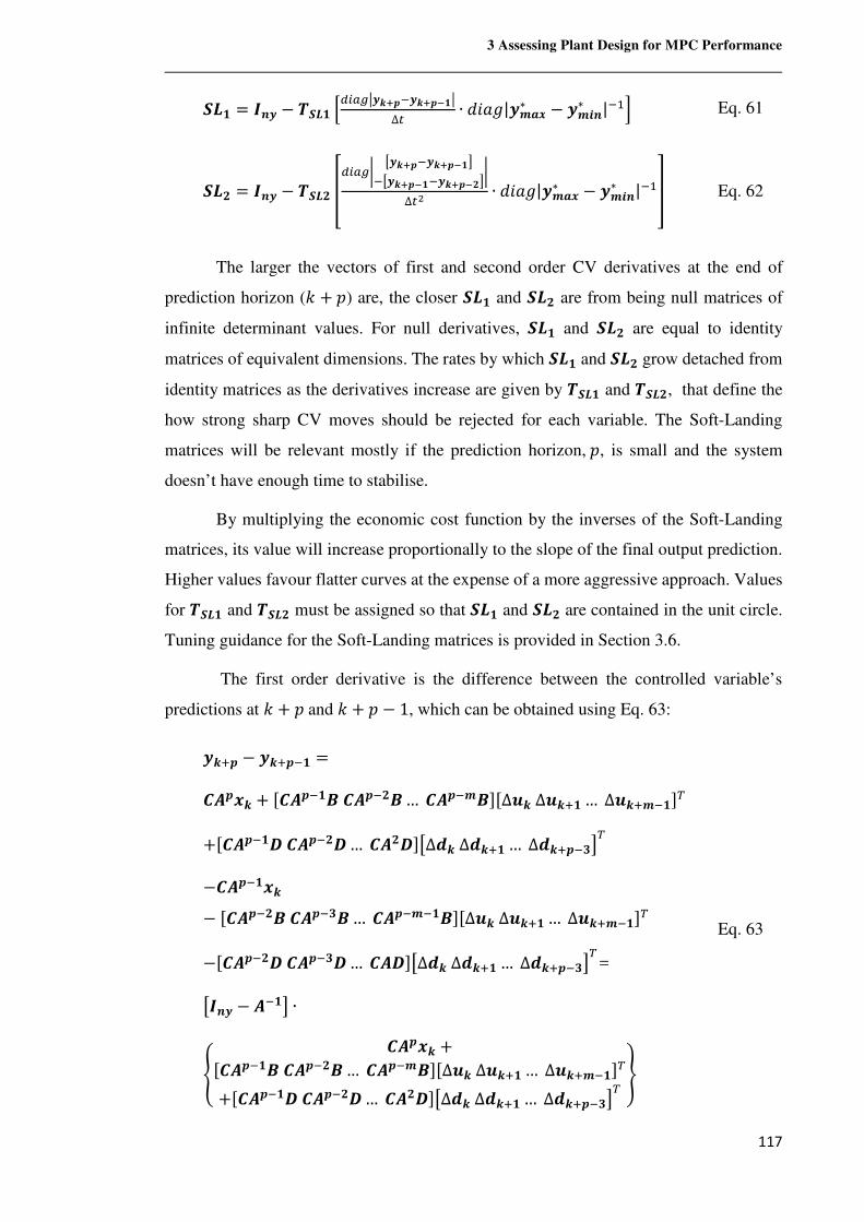
3 Assessing Plant Design for MPC Performance
117
_`� = �h� − b_`� >,'??Ø�\*Y.�\*Y@�Ø∆@ ∙ ë¹~A|���∗ − ��Vh∗ |.�C Eq. 61
_` = �h� − b_` ,'??D &�\*Y.�\*Y@�(.&�\*Y@�.�\*Y@ (D
∆@p ∙ ë¹~A|���∗ − ��Vh∗ |.�" Eq. 62
The larger the vectors of first and second order CV derivatives at the end of
prediction horizon (� + �) are, the closer _`� and _` are from being null matrices of
infinite determinant values. For null derivatives, _`� and _` are equal to identity
matrices of equivalent dimensions. The rates by which _`� and _` grow detached from
identity matrices as the derivatives increase are given by b_`� and b_` , that define the
how strong sharp CV moves should be rejected for each variable. The Soft-Landing
matrices will be relevant mostly if the prediction horizon,�, is small and the system
doesn’t have enough time to stabilise.
By multiplying the economic cost function by the inverses of the Soft-Landing
matrices, its value will increase proportionally to the slope of the final output prediction.
Higher values favour flatter curves at the expense of a more aggressive approach. Values
for b_`� and b_` must be assigned so that _`� and _` are contained in the unit circle.
Tuning guidance for the Soft-Landing matrices is provided in Section 3.6.
The first order derivative is the difference between the controlled variable’s
predictions at � + �and � + � − 1, which can be obtained using Eq. 63:
�\|Y − �\|Y.� =
��Y\ + µ��Y.����Y. �… ��Y.��·µ∆�\∆�\|�…∆�\|�.�·%
+µ��Y.� ��Y. … �� ·&∆�\∆�\|�…∆�\|Y.'(%
−��Y.�\− µ��Y. ���Y.'�… ��Y.�.��·µ∆�\∆�\|�…∆�\|�.�·%
−µ��Y. ��Y.' … �� ·&∆�\∆�\|�…∆�\|Y.'(%=
&�h� − �.�( ∙ E ��Y\ +µ��Y.����Y. �… ��Y.��·µ∆�\∆�\|�…∆�\|�.�·%+µ��Y.� ��Y. … �� ·&∆�\∆�\|�…∆�\|Y.'(% ;
Eq. 63
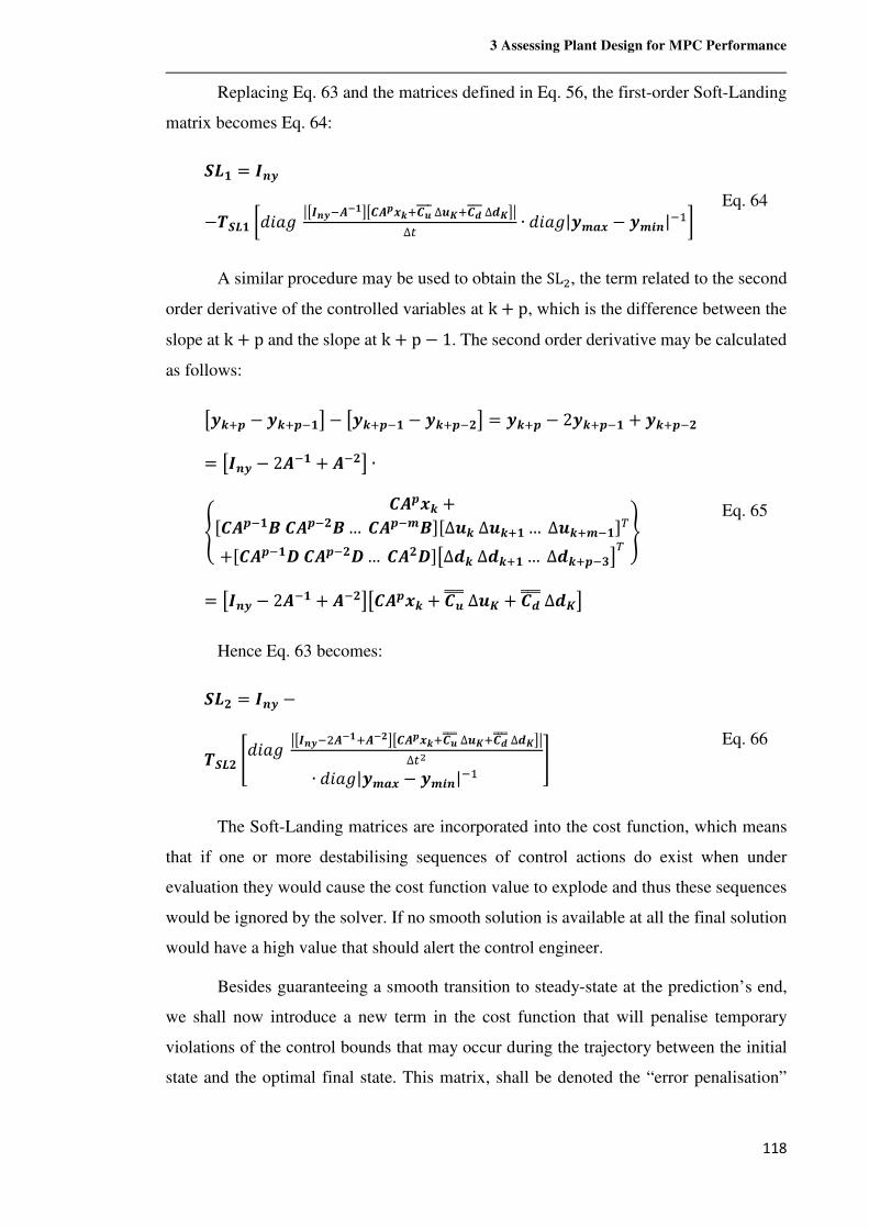
3 Assessing Plant Design for MPC Performance
118
Replacing Eq. 63 and the matrices defined in Eq. 56, the first-order Soft-Landing
matrix becomes Eq. 64:
_`� = �h�
−b_`� #ë¹~A Ø&�h�.�@�(&��Y\|������∆�!|������∆�!(Ø∆@ ∙ ë¹~A|��� − ��Vh|.�$ Eq. 64
A similar procedure may be used to obtain the SL�, the term related to the second
order derivative of the controlled variables at k + p, which is the difference between the
slope at k + p and the slope at k + p − 1. The second order derivative may be calculated
as follows:
&�\|Y − �\|Y.�(− &�\|Y.� − �\|Y. ( = �\|Y − 2�\|Y.� + �\|Y.
= &�h� − 2�.� + �. ( ∙ E ��Y\ +µ��Y.����Y. �… ��Y.��·µ∆�\∆�\|�…∆�\|�.�·%+µ��Y.� ��Y. … �� ·&∆�\∆�\|�…∆�\|Y.'(% ;
= &�h� − 2�.� + �. (&��Y\ + ������∆�! + ������∆�!( Eq. 65
Hence Eq. 63 becomes:
_` = �h� −
b_` 7ë¹~A Ø&�h�.��@�|�@ (&��Y\|������∆�!|������∆�!(Ø∆@p
∙ ë¹~A|��� − ��Vh|.� : Eq. 66
The Soft-Landing matrices are incorporated into the cost function, which means
that if one or more destabilising sequences of control actions do exist when under
evaluation they would cause the cost function value to explode and thus these sequences
would be ignored by the solver. If no smooth solution is available at all the final solution
would have a high value that should alert the control engineer.
Besides guaranteeing a smooth transition to steady-state at the prediction’s end,
we shall now introduce a new term in the cost function that will penalise temporary
violations of the control bounds that may occur during the trajectory between the initial
state and the optimal final state. This matrix, shall be denoted the “error penalisation”
3 Assessing Plant Design for MPC Performance
119
matrix (EP) and it will increase the cost function value if any of the controlled variables
stay out of their control zone.
Definition 3.5.2 Error-Penalisation matrix. Let bcR<ℝ*� be a parameter
vector that define the priority of rejecting control zone bound violations for
each CV, � be an auxiliary variable that denotes time during the transient,
whose value varies from � = � (beginning of the prediction horizon) to � =� + � (end of the prediction horizon), �G<ℝ*� be the vector of controlled
variables at time alpha, and ���<ℝ*� and ��Vh<ℝ*� be vectors
denoting the upper and lower control zone bounds, b�YY�T,G<ℝ*� and
b�de�T,G<ℝ*� be parameter vectors that define, respectively, the active
upper and lower control zone bounds at time alpha, where MQ is the number
of CVs. The Error-Penalisation matrix cR<ℝ*��*� is defined by Eq. 67.
cR = �h� −
bcR∑ Hµë¹~Ak�|��� − ��Vh|m·.� ∙ ë¹~A I |�G − ���| ∙ b�YY�T,G+|��Vh − �G| ∙ b�de�T,GJK(|NL/(
Eq. 67
So �G is compared to ��� and ��Vh throughout the transient to assess if any CV
left its control zone. When obtaining solutions to the EMOP optimisation problem, the
restrictions to b�YY�Tand b�de�T shown in Eq. 68 to Eq. 70 must be included.
¹+w',�'* ≤ w(|N,',L ≤ w',�?� ⇒ a',PNNLH = a',)K�LH = 0 Eq. 68
¹+w',�'* > w(|N,',L ⇒ a',)K�LH > 0 Eq. 69
¹+w(|N,',L > w',�?� ⇒ a',PNNLH > 0 Eq. 70
These restrictions guarantee that cR will decrease if, during the transient, any
controlled variable overshoots. If that happens, the solution will be penalised even if the
final state is within its control zone. Matrices b�de�T, b�YY�T and bcR define how strongly
overshooting will be rejected, but they must be small enough to guarantee that cR > ¾
through all the transient response.
Finally, we can reach the complete form for the EMOP index by multiplying the
cost function given by Eq. 59 by the inverse of the determinants of the Soft-Landing and
the error penalisation matrices, _`�, _` and cR.
3 Assessing Plant Design for MPC Performance
120
Definition 3.5.3 The Economic MPC Optimisation index. In the complete
form of the EMOP index, the optimisation problem of Eq. 60 is replaced by
the one defined by Eq. 71, which includes the effects of _`�, _` and cR.
23456 = �¹M∆�!∈g
Ô|_`�|.�|_` |.�&;(|N + |cR.�|(Ö Eq. 71
The desired outcome is that, for the selected plant design, the impact of
matrices_`�, _` and cR on the Economic MPC Optimisation index will be very small.
Should these matrices affect the EMOP index in a remarkable way, it would be a sign that
either their tuning is too aggressive or that the flowsheet is rather inappropriate. In a
typical use scenario, the optimal value is mostly a consequence of the control actions
necessary to offset the effects of DVs, changes in the control zones or changes in
economics parameters. Hence, the standard index formulation of Eq. 71 should cause the
optimisation solver to discard solutions which present significant overshooting. A good
solution for the EMOP problem guarantees that eventual violations of control zones are
quick enough to keep the effects of the EP matrix relatively small.
If the plant is stable and if the prediction horizon p is sufficiently larger than the
control horizon �, control actions will already have taken full effect by the end of the
prediction, � + �, and hence _`� and _` will be nearly identity matrices. In turn, this
means the EMOP index refers to a steady state. If, however, if � is small the index cost
function will increase, and the solution will be penalised heavily.
3.6 EMOP Index Interpretation and Tuning
So how can we interpret the Economic MPC Optimisation index? The index is
indirectly related to properties such as controllability, flexibility, operability, feasibility
and switch ability, but it provides results directly related to the economics of the process.
Specifically, the EMOP index is measured by monetary units such as US dollars and is
strongly linked to plant operating revenue. The feedback from this methodology enables
the control engineer to validate changes in the flowsheets and assess their impact on
controllability and profitability.
What is being measured by the index? It quantifies the effects of key process
design choices in the capacity of the MPC controller to avoid economic losses, providing
a measure of how much a plant can be optimised while keeping controlled variables
within the bounds of the zone control. The first two terms in Eq. 59 penalise any plant
3 Assessing Plant Design for MPC Performance
121
whose optimal steady-state lies outside the bounds defined by zone control for one or
more CVs. Typical MPC CVs be classified into two categories:
• Product specifications, e.g., the purity grade of a chemical product;
• Operation specifications, e.g., combustion chamber pressure of a fired
heater.
Products specifications are directly related to process economics since off-spec
products have lower market value or even no value at all. Operation specifications are
normally indirectly related to process economics, acting as restrictions to process
optimisation. One exception would be catalyst temperature, which is related to
deactivation rate and thus can be linked to monetary loss.
Manipulated variables sometimes can also be linked to manufacturing costs or
revenue. Some examples of MVs with a strong relation to process economics include:
• Feed flow rate;
• Product output;
• Energy supply, e.g., electricity, natural gas, etc.;
• Product recycles;
• Pumparound Duty (energy saved due to feed preheating).
The third and fourth terms in Eq. 59 penalise the gap between optimal MV value
and the final steady-state value and may be interpreted as being the MV opportunity cost.
The steady state is key in the analysis since it is where the plant is expected to operate
during most of the time. However, it is also necessary to evaluate how the plant behaves
during state transitions. It is of special importance to ascertain that environmental and
safety CVs do not overshoot during the transient, as even small violations can have a
significant negative impact. Eq. 67 was added to the index to penalise constraint
violations as it is driven to the optimal state. Eq. 61 and Eq. 62 were added to promote
control actions that result in smooth plant responses. If the Soft-Landing matrices
(_`�and_` ) and the error penalization matrix (cR) are small this will cause the EMOP
index to increase, reflecting a poor dynamic response. The magnitude of this penalisation
depends on decisions made by the project team concerning which CVs must be prioritised
and what harm can be brought by eventual constraint violations.
The vectorsb_`�, b_` ,bcR, b�YY�T and b�de�T all require manual tuning. Their
values should reflect prioritisation among controlled variables as well the desired balance
between steady-state optimisation and penalisation for eventual issues in the transient
3 Assessing Plant Design for MPC Performance
122
behaviour. The larger the values, the greater the penalties for lack of a smooth transition
to the final state and violations of the control zones. The exact values that should be
assigned depending on the number of variables (a larger number of variables increases
their cumulative effect) and the desired penalty. For example, one could tune bcR, b�YY�T and b�de�T in such a way that |cR|.� = ;(|N ∙ &0.5 MQ⁄ (, if a single variable stays
unbounded for 50% of the transient. If in addition to that another variable is unbounded
for 75% of the transient, |cR|.� = ;(|N ∙ &k0.5+ 0.75m MQ⁄ (, and so on. Another
possibility is setting b_`� and b_` in such a way as to provide Soft-Landing matrices
that follow, approximately, |_`�|.� = ;(|N ∙ �∏ O1 + �\|Yy �\|Y⁄Mw − 1� and |_` |.� =;(|N ∙ �∏ O1 + �\|Yyy �\|Y⁄Mw − 1�. While these are useful guidelines, the tuning choices
ultimately depend on the control engineer’s judgement about the correct balance between
steady-state and transient performances, both of which are important elements of the
analysis. The concept of “optimal tuning” does not apply here: what is necessary is that
the selection of tuning parameters reflects adequately the criteria by which process
performance is going to be judged. The parameters must be the same for all flowsheets
resulting in the use of the same criterion.
3.7 Including price variations in the EMOP cost function
In some processes, the market prices of one or more products are related to key
CVs. Just to name two relevant examples, petrol (gasoline) and diesel oil are priced in the
global market according to, respectively, their Octane Number and Cetane Index. Also,
numerous inorganic chemical processes have their products priced according to their
degree of purity. Therefore, the possibility of producing premium as opposed to regularly
priced products should be incorporated into the EMOP index’s cost function. To
accomplish that, a new term is added to the cost function for each product price variation.
This new term is a function of a new variable, ∆������, defined as the difference between
the key CV quality threshold value for which the price variation occurs, ������, and the
average value of the key CV through the prediction horizon, �����, as shown in Eq. 72
and Eq. 73:
¹+Ô������ − �����Ö ≥ ¾, ∆������ = Ô������ − �����Ö Eq. 72
¹+Ô������ − �����Ö < ¾, ∆������ = ¾ Eq. 73
So, the added cost function value, j�, is defined as:
3 Assessing Plant Design for MPC Performance
123
Õ� = ∆������ ∙∆R�����YTd�
∙ �YTd� Eq. 74
Where ∆R���� is the added value, i.e., product price difference between premium
priced and regular product, and �YTd� is the volume produced of said product. If there are
more than one quality threshold for a single CV, adding the price increments of all the
consecutive thresholds to the price of the regular product, RT�0, should yield the price of
the most premium variant, R����,h�, as shown in Eq. 75:
R����,� = RT�0 + ∆R����,�
⋮
R����,h� = RT�0 + ∑ ∆R����,Õh�Õ/� Eq. 75
Where nq is the number of quality thresholds of the product being considered. For
processes with several CVs with quality thresholds, it is useful to aggregate all added cost
function values in a single term, as per Eq. 76:
;> = ∑ ∑ ∆w�>P?),' ∙∆6P�QR,x,�J+ST�,� ∙ UNHK,,'*>,'
Ý/�*Q'/� Eq. 76
Where ;> is total opportunity cost due to quality thresholds. This way, ;> becomes
null if only the most premium priced product variants are being produced. Adding to Eq.
71, the EMOP index becomes:
23456 = �¹M∆PV∈8Ô|_`�|.�|_` |.�&;(|N + ;> + |cR.�|(Ö Eq. 77
3.8 Exploring the Relation between the Regulatory Control Layer, MPC
Layer and the EMOP Index
The approach presented in this Thesis is based on the premise that DVs are known
and estimated a priori and follow a given time-dependent profile. While this may seem
restrictive, this choice reflects the nature of the dual layer control strategy used, where
the MPC is used for economic optimisation, and feedback controllers deal with fast
disturbances.
Also, that in many chemical processes often the MPC layer DVs are known and
planned ahead of time by operating staff. Examples of MPC layer DVs include events
such as changes in the feed composition and product specifications, programmed
3 Assessing Plant Design for MPC Performance
124
equipment shutdowns, tank switches, and changes in pipeline alignment. Here we
compare for each plant how planned one-off occurrences, which are very frequent and
impact process profitability. DVs that may be modelled stochastically, such as
observational noise, are normally dealt with by the regulatory control layer, which is
much faster. The control engineer must keep in mind that the regulatory layer is part of
the plant which is being evaluated and modifying it changes the model and analysis
results.
This Thesis does not concern the issue of the selection of the lower level control
structure, i.e., selecting MVs and CVs for regulatory control and dealing with their
interconnections. This important subject has already been investigated in Kookos and
Perkins (2001) and Kookos and Perkins (2012), among others (a review of methods for
input/output selection is presented in De Wal and Jager, 2001). For the EMOP index
method, it is enough to assume that the plant is Integral Controllable and the embedded
control structures of each flowsheet were correctly engineered and tested, yielding
controllable plants. If this assumption is correct, the tuning of the lower level control
structure will not affect the EMOP index significantly.
For instance, in the case study provided in Section 4, the linear models that define
each plant are closed-loop models involving multiloop feedback controllers. The sample
time used for the state-space models was 10 minutes while PID controller sample time
was set at 1 second at the simulation. The large difference in speed between MPC and
PID variables greatly diminishes the index sensitivity to the regulatory control structure.
Tests showed that the PIDs could bring its CVs back to their SPs easily and rapidly when
the process was disturbed. Also, these PIDs proved themselves easy to tune and had
excellent performance for all plants. And finally, the issue of feedback control structures
for crude oil distillation has been adequately tackled in sources such as Luyben (2013)
and Brambilla (2014), providing templates that could be embedded in the flowsheets. So,
in this case, the effect of the regulatory control layer was small enough to be safely
ignored.
However, this may not always be the case. If there is no clarity over the selection
of control structure, or if one or more flowsheets are not Integral Controllable, then the
design and tuning of the lower layer may have an impact on the EMOP index. A bad score
may help to detect, for example, if the regulatory control is tuned too slowly or
aggressively, or if its actuators run at their saturation limits, etc., but should such issues
be detected, the flowsheet should be discarded.
3 Assessing Plant Design for MPC Performance
125
3.9 Using the EMOP index to compare plants with radically different
layouts
So far in this work, we focused on comparing flowsheets which share main
characteristics and have enough similarity to possess the same MPC structure, i.e., the
same set of CVs and MVs. Additionally, in our study case in Chapter 6, the same control
zones were used for all plants, and all of them started the simulation at the same (null)
state. Having the same control zones, optimisation weights and initial states greatly
facilitates the flowsheet assessment. The effects of comparatively small design
differences can be thus evaluated. But there may be situations where we desire to compare
plants for which these assumptions are not accurate. During the early stages of chemical
process design, it may be necessary to choose between the different routes and
technologies available to produce a certain product. For instance, some different routes
for methanol production exist, including synthesis from oil, natural gas or coal. It is
unlikely that these candidate flowsheets will share the same MPC structure.
So here a new parameter is introduced in the EMOP index as a means to enable
comparison between plants that have each its own control bound definitions and starting
point, MVs, CVs and parameters. This extended EMOP index can be used to compare
completely different plants.
The EMOP index is a measure of monetisation of the control effort, and it
calculates changes in operating revenue caused by control actions and disturbances. One
basic assumption until now, besides shared MPC structure, is that all flowsheet designs
have the same expected operating revenue at the initial operating point. For instance, all
crude oil distillation plants described in Chapter 4 have the feed flowrate, the same oil
mix, and produce the same products at the start of the simulation. Therefore, all plants
began the simulation with the same operating revenue.
This basic assumption will not, of course, be correct for designs that use different
production routes, raw materials, MPC control structures, etc. So, in this case, the distinct
initial operating revenue of each plant must be account for. Let us subtract operational
revenue (total sales minus costs) at an initial time k�m from the EMOP index definition,
Eq. 77, yielding Eq. 78:
3 Assessing Plant Design for MPC Performance
126
23456,6W =
�¹M∆�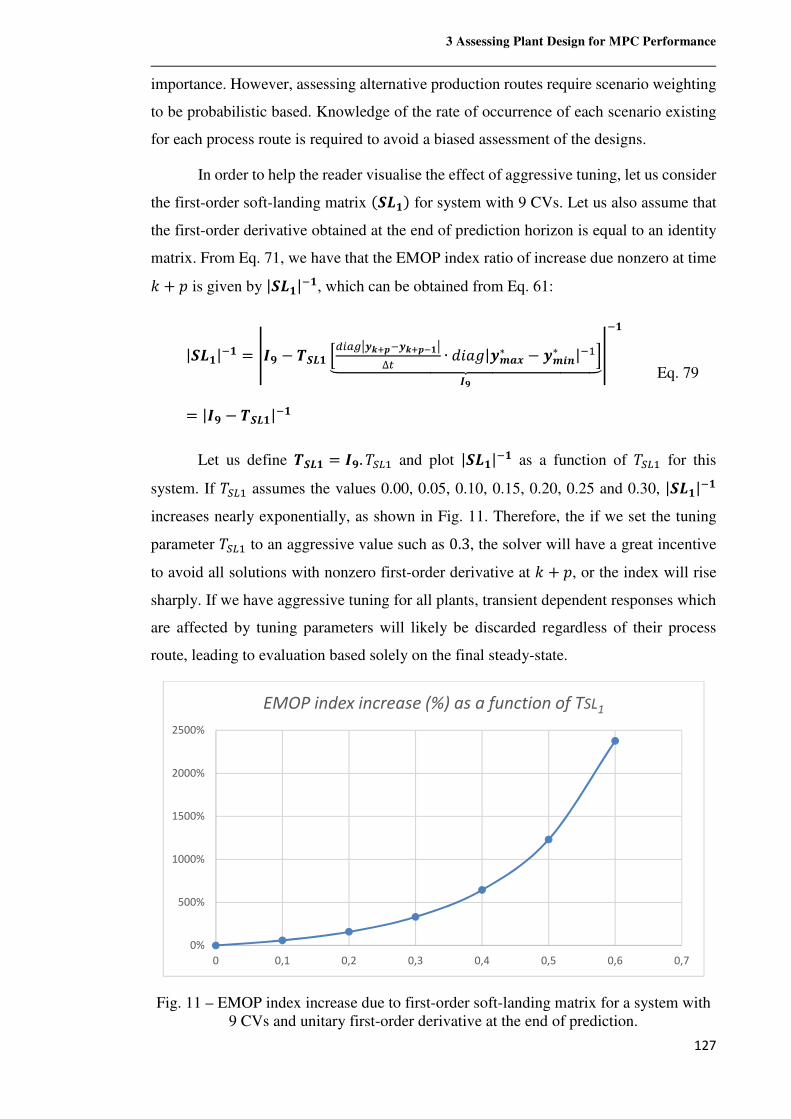
3 Assessing Plant Design for MPC Performance
127
importance. However, assessing alternative production routes require scenario weighting
to be probabilistic based. Knowledge of the rate of occurrence of each scenario existing
for each process route is required to avoid a biased assessment of the designs.
In order to help the reader visualise the effect of aggressive tuning, let us consider
the first-order soft-landing matrix k_`�m for system with 9 CVs. Let us also assume that
the first-order derivative obtained at the end of prediction horizon is equal to an identity
matrix. From Eq. 71, we have that the EMOP index ratio of increase due nonzero at time
� + � is given by |_`�|.�, which can be obtained from Eq. 61:
|_`�|.� = [�\ − b_`� >,'??Ø�\*Y.�\*Y@�Ø∆@ ∙ ë¹~A|���∗ − ��Vh∗ |.�CÇÈÈÈÈÈÈÈÈÈÈÈÈÉÈÈÈÈÈÈÈÈÈÈÈÈÊ�\
[.�
= |�\ − b_`�|.�
Eq. 79
Let us define b_`� = �\. a]é� and plot |_`�|.� as a function of a]é� for this
system. If a]é� assumes the values 0.00, 0.05, 0.10, 0.15, 0.20, 0.25 and 0.30, |_`�|.�
increases nearly exponentially, as shown in Fig. 11. Therefore, the if we set the tuning
parameter a]é� to an aggressive value such as 0.3, the solver will have a great incentive
to avoid all solutions with nonzero first-order derivative at � + �, or the index will rise
sharply. If we have aggressive tuning for all plants, transient dependent responses which
are affected by tuning parameters will likely be discarded regardless of their process
route, leading to evaluation based solely on the final steady-state.
Fig. 11 – EMOP index increase due to first-order soft-landing matrix for a system with 9 CVs and unitary first-order derivative at the end of prediction.
0%
500%
1000%
1500%
2000%
2500%
0 0,1 0,2 0,3 0,4 0,5 0,6 0,7
EMOP index increase (%) as a function of TSL1
3 Assessing Plant Design for MPC Performance
128
3.10 Conclusions concerning the EMOP index
In brief, the EMOP index methodology can be considered as a state reachability
problem that deals with zone restrictions, disturbances, smoothness of the transient
response and process economics. Details of the concept of state reachability can be found
in Vidyasagar (2002). As a way of recapping the contents of this Chapter, let us now
outline the EMOP index’s main features:
• The EMOP index measures the impact of process dynamics in the OPEX;
• To this end, zone constrained MPC with economic capabilities is assumed;
• The optimised EMOP index determines what are the most profitable and
yet reachable state, and does so evaluating just how much room for
optimisation is available. The lower the index, the better the state
reachability for a given plant;
• The index is used to assess how well-suited a flowsheet is to accommodate
disturbances while being and controlled and optimised by any MPC,
allowing comparison between different process plants;
• The required control effort and the achievable control performance are
measured in the face of a set of disturbances and zones constraints. For
any adequate plant design, at least one set of control actions exists that
successfully rejects disturbances while economically optimising the
process;
• Control performance is monetised by measuring the revenue changes
caused by the control actions adopted and bound violations of
environmental restrictions and product specifications, i.e., the index must
account for the eventual economic losses due to the necessary control
actions;
• The index indicates the best achievable control performance from a broad
economic and stability standpoint. As it is always the case for
Controllability Analysis, it only depends on the plant’s own characteristics
and control goals, independently of the MPC algorithm and tuning
parameters that will be eventually used to control these plants;
• The index provides a workable solution for assessing control performance
and its economic ramifications for moderately complex plants (or a key
section of a highly complex process unit, i.e., reactional section,
distillation column, heat exchanging section, etc.);

3 Assessing Plant Design for MPC Performance
129
• The EMOP index ranking of the candidate plant designs shows how they
compare in terms of resilience to disturbances, controllability, product
quality giveaway and costs.
Considering the contributions above, one could argue that the EMOP index differs
significantly from the existent body of work of integrated process design and control
methods. Its innovation also comes from the fact that it is not intended to replace other
methods, but to be used alongside them as a decision-making tool.
4 The simultaneous multi-linear prediction
130
4 The simultaneous multi-linear prediction
The assessment of control performance of large-scale systems uses data from
commercial, black-box nonlinear dynamic simulation packages that are popular in the
chemical industry. These state-of-the-art simulators are the tools of choice of most
process design teams. We use the integrated design and control approach for large-scale,
complex processes for which the full set of equations is unavailable.
Data from one such simulator was used in Strutzel and Bogle (2016) to identify
linear state-space models that predicted the dynamic behaviour of each flowsheet. This is
a better option than using the nonlinear simulation package directly since that is very
computationally intensive. However, using linear models to predict the behaviour of
nonlinear plants is inevitably going to result in some error. This problem was addressed
by defining the EMOP index as an interval (bounded by best and worst scenarios) within
which the true controllability index must be contained.
In this Thesis, an alternative approach for reducing nonlinearity-introduced error
is presented while keeping all the advantages of using linear models. This solution, a new
multi-model state-space approach called Simultaneous Multi-Linear Prediction (SMLP),
is described in the following Sections. The main idea is to ensure that the evaluation of
the index and the subsequent ranking of flowsheets are as accurate as possible within a
reasonable timeframe, thus rendering the EMOP index more resilient to process
nonlinearity. While not the focus of this Thesis, the SMLP can also be used for process
control purposes and for MPC in particular, since its open loop stability can be guaranteed
as we will show.
A major part of MPC’s appeal in industry stems from the use of a linear finite step
response model of the process and a quadratic objective function. When MPC is
employed on processes with significant nonlinearity, the application of a linear model-
based controller may have to be limited to relatively small operating regions. Specifically,
since the computations are entirely based on the model prediction, the accuracy of the
model has a significant effect on the performance of the closed-loop system (Gopinath et
al, 1995). Hence, the capabilities of MPC will degrade as the operating level moves away
from its original design level of operation (Dougherty and Cooper, 2003). Enhancing
4 The simultaneous multi-linear prediction
131
prediction accuracy will increase closed-loop stability and help avoid overdamped or
underdamped responses.
MPC for SMLP also has one advantage over MPC with nonlinear models
(NMPC): while NMPC may involve non-convex optimisation problems for which local
minima can found but nothing can be said about the global minimum (Kantner and
Primbs, 1997), the use of an SMLP prediction provides a convex cost function for which
the global minimum can be easily found without the need for relaxation.
As discussed in Section 2.4, PieceWise Affine (PWA) systems are popular
methods for obtaining multi-model linear approximations of nonlinear systems.
Nevertheless, PWA approximations have some issues that keep them from being the ideal
solution for use with integrated process design and control approaches: firstly, the
availability of the full set of equations of the nonlinear model is a requirement for existing
PWA methods. This is not going to be the case if most of the commercial simulation
packages are to be used.
While it is relatively straightforward to employ a standard PWA approach to
identify step response models, a good approximation of the nonlinear simulation package
cannot be guaranteed. The clustering technique (Ferrari-Trecate et al., 2003) and the
“point-to-point” method (Lowe and Zohdy, 2010) which are used to identify optimal
partitions for PWA systems depend on the availability of a full set of differential
equations describing the process. Alternatively, an explicit expression for probability
density of the data can be used (Nakada et al. 2005). If this condition is not met, then any
partition definition will necessarily be arbitrary since it will be dependent on the starting
point of the identification data. Both the choice of linearisation points and boundaries will
not be optimal, and the PWA identification problem becomes finding the best fit to the
available data. In this situation, the only way one could ensure that a modified PWA
scheme would provide an adequate approximation would be through the use of numerous
models valid for small regions, if data is available from several starting points.
This leads to the second issue: it is desirable to have a multi-model class capable
of reliable and accurate prediction by using only a small number of sub-models. If the
necessary number of partitions is high, the process of data-based model identification is
very laborious and time-demanding. This is true when the data is provided by dynamic
simulators but even more so when we desire to control an existing chemical plant.
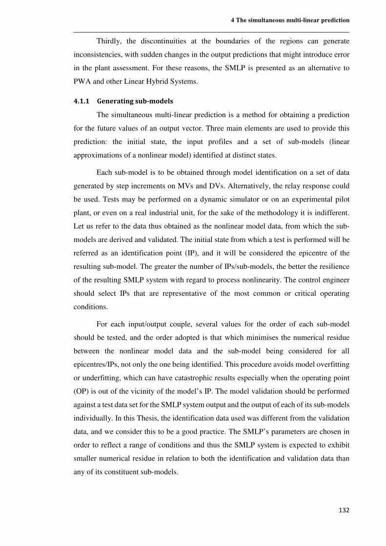
4 The simultaneous multi-linear prediction
132
Thirdly, the discontinuities at the boundaries of the regions can generate
inconsistencies, with sudden changes in the output predictions that might introduce error
in the plant assessment. For these reasons, the SMLP is presented as an alternative to
PWA and other Linear Hybrid Systems.
4.1.1 Generating sub-models
The simultaneous multi-linear prediction is a method for obtaining a prediction
for the future values of an output vector. Three main elements are used to provide this
prediction: the initial state, the input profiles and a set of sub-models (linear
approximations of a nonlinear model) identified at distinct states.
Each sub-model is to be obtained through model identification on a set of data
generated by step increments on MVs and DVs. Alternatively, the relay response could
be used. Tests may be performed on a dynamic simulator or on an experimental pilot
plant, or even on a real industrial unit, for the sake of the methodology it is indifferent.
Let us refer to the data thus obtained as the nonlinear model data, from which the sub-
models are derived and validated. The initial state from which a test is performed will be
referred as an identification point (IP), and it will be considered the epicentre of the
resulting sub-model. The greater the number of IPs/sub-models, the better the resilience
of the resulting SMLP system with regard to process nonlinearity. The control engineer
should select IPs that are representative of the most common or critical operating
conditions.
For each input/output couple, several values for the order of each sub-model
should be tested, and the order adopted is that which minimises the numerical residue
between the nonlinear model data and the sub-model being considered for all
epicentres/IPs, not only the one being identified. This procedure avoids model overfitting
or underfitting, which can have catastrophic results especially when the operating point
(OP) is out of the vicinity of the model’s IP. The model validation should be performed
against a test data set for the SMLP system output and the output of each of its sub-models
individually. In this Thesis, the identification data used was different from the validation
data, and we consider this to be a good practice. The SMLP’s parameters are chosen in
order to reflect a range of conditions and thus the SMLP system is expected to exhibit
smaller numerical residue in relation to both the identification and validation data than
any of its constituent sub-models.
4 The simultaneous multi-linear prediction
133
4.1.2 Introducing the Simultaneous Multi-Linear Prediction (SMLP)
In this Section, the novel multiple state-space model method, Simultaneous Multi-
Linear Prediction (SMLP), is presented. Its role is to reduce the nonlinearity-related error
and avoid discontinuities between approximated regions. The SMLP avoids
discontinuities by avoiding partitions and changes in the state update equation through
the whole space of feasible operating points. Instead of a single state vector as found in
Linear Hybrid Systems such as PWA, the SMLP uses multiple sub-state vectors
calculated simultaneously, one for each linear state-space sub-model. Note that since
these model matrices do not share the same state vector, they need not possess the same
dimensions (a requirement for PWA systems). In the SMLP, all sub-states to some degree
contribute to the main output at all times, as shown in Fig. 12:
Fig. 12 – The output prediction can be generated by multiple simultaneous states, each one with its own update rule (SMLP system), or by a single state which continuously
changes update rule (PWA system).
Each sub-state creates an output rate of change vector, and the result of the
weighted addition of these vectors will generate the main output. The contribution ratio
of each component is defined by a weight parameter, itself a function of three factors: the
current position of the operating point; the points where each sub-model was originally
identified (known as identification points or IPs); and a set of parameters obtained through
linear regression to minimise the gap between the SMLP output and the simulator.
...
...
The SMLP Output, w, is
yielded by weighted average
of all sub-model outputs
I�
I�
I*_
u��
u�p
u�#_
SMLP
M�
M�
Mý`
u w
PWA
...
...
...
...
An SMLP system is made of a set
of M� sub-models. Each has its
own state and output vectors.
w��
w�p
w�#_
...
A PWA system has a single state
and output vectors, which are
updated by M� sub-models. Only
one sub-model is active at a time,
according to the location of the
state in the partitioned state-space.
4 The simultaneous multi-linear prediction
134
The SMLP does not assume that one particular sub-model has priority over others
within an arbitrary partition of the input space. Without being restricted to any arbitrary
bounds, the weight parameters change freely inside the whole space with a view to
minimising the nonlinearity error. Besides avoiding discontinuities, eliminating partitions
may provide a gain in accuracy since the search for optimal parameters becomes an
unconstrained optimisation problem.
Three variants of the SMLP methodology have been devised by considering two
different definitions of operating point (or OP) and two options for parametrisation
obtained through regression analysis. In the first SMLP variant, the OP is the output (CV)
vector kym, whereas for the other two variants the OP is the input vector kµud·m combining
manipulated and disturbance variables (MVs and DVs). The first definition is appropriate
when the CVs can be known precisely and updated regularly, and when there are no time
delays or non-stationary (integrating) variables such as levels. On the other hand, OP can
always be expressed as an MV vector since MVs are defined by the control system and
are thus readily available. Measured disturbance variables (DVs) should also be
incorporated in the OP.
As for the parametrisations, the two options consist of either having a single set
of parameters for each multivariable sub-model, which will be called MIMO
parametrisation or having a separated set for each pair of output/input, called SISO
parametrisation, which may yield an improved prediction. A key disadvantage of the
SISO parametrisation as compared to the MIMO parametrisation is the increased time
required to perform the regression analysis, as it is individually done for each CV/MV or
CV/DV pair. This trade-off is significant if the number of variables is high.
4.1.3 SMLP Method 1 – the MIMO parametrisation
The Simultaneous Multi-Linear Prediction (SMLP) is a method for obtaining a
prediction for the future values of an output vector. Three main elements are used to
provide this prediction: the initial state, the input profiles and a set of sub-models (linear
approximations of a nonlinear model) identified at distinct states.
Let us first outline the SMLP method for the special case of an output vector with
two variables, ��and � , which are to be controlled for a defined set of disturbances.
Consider that, for a given flowsheet, model identification was performed at two
identification points, �R� = &w�,a6� , w�,a6�( and �R = &w�,a6p , w�,a6p(, yielding
4 The simultaneous multi-linear prediction
135
respectively sub-models � and that are Taylor approximations of the nonlinear
model.
The SMLP formulation makes use of a standard linear state-space formulation
presented in Lee et al. (1994). The sub-models � and are systems of equations
defined, respectively, by the state-space matrices ���, ���,��� and �� and �� , �� ,�� and � , as well as by state vectors of appropriate dimensions, \�� and \� , where � is the time at initial conditions. The state vectors \�� and \� are henceforth
called simultaneous sub-states since they evolve independently from each other, being
subject to the same set of control actions (�\, �\|�, … , �\|�, where � is the number of
control actions) through the control horizon, and also to the same set of disturbances
(�\, �\|�, … , �\|Y, where � is the length of the prediction) through the entirety of the
prediction horizon. Hence, each sub-model has a sub-state update equation in the
incremental form, as shown in Eq. 80 and Eq. 81:
\|��� = ���\�� + ���∆�\ + ��∆�\ Eq. 80
\|�� = �� \� + �� ∆�\ + � ∆�\ Eq. 81
Where ∆�\ = µ�\ − �\.�·% and ∆�\ = µ�\ − �\.�·%. Therefore, even though
the inputs are the same for both sub-models, different values for next-instant sub-states,
\|��� and \|�� , are obtained as well as different output predictions, respectively �\�� and
�\� for � and , as shown in Eq. 82 and Eq. 83:
�\�� = ���\�� Eq. 82
�\� = �� \� Eq. 83
Let us define the operating point (OP) at time � as being the output vector of the
multi-model system, i.e., ±R\ = &w�,(, w�,((. Note that usually ±R\ ≠ �\�� ≠ �\� . Due
to nonlinearity effects, the model � is expected to get less accurate the further the
operating point ±R is removed from the first identification point �R�. In other words, if
the plant is operated close to an identification point, its modelling error will probably be
small. This should be valid as a general trend even if untrue at some points. So, it makes
sense that the weights of � and are roughly inversely proportional to, respectively,
the distance in the Euclidean MQ-space between points �R� and ±R\ k�R�±R\�����������m and
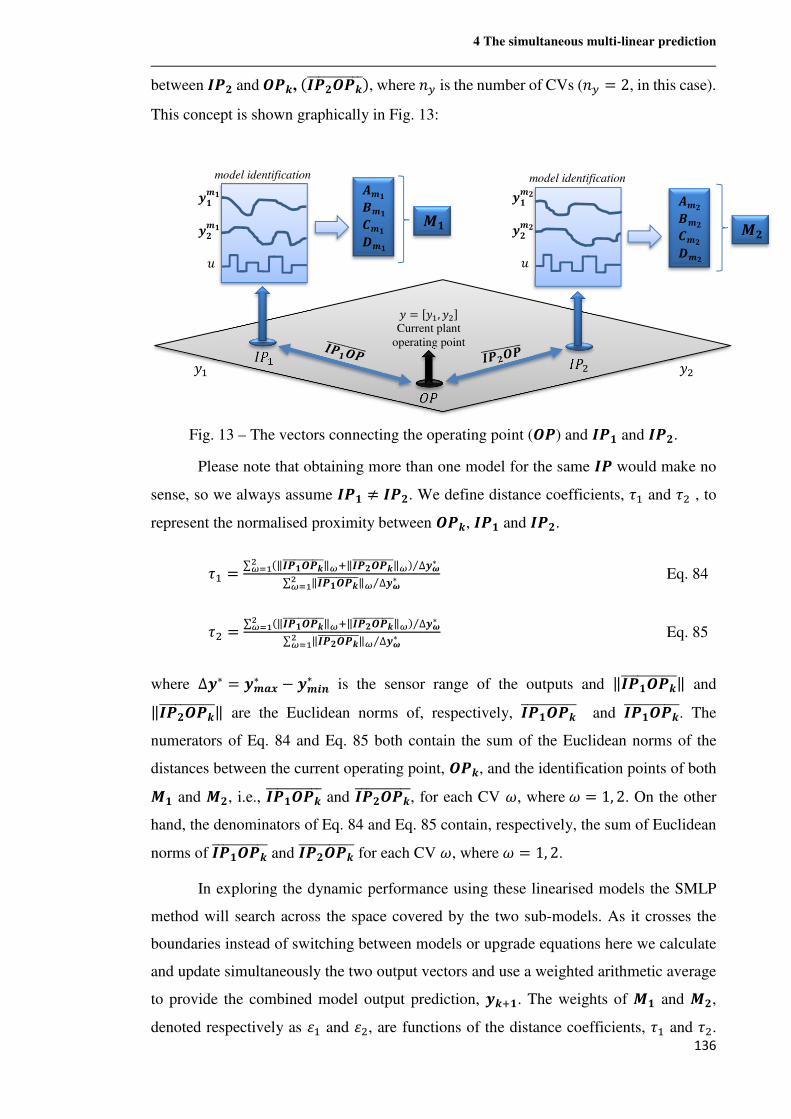
4 The simultaneous multi-linear prediction
136
between �R and ±R\, k�R ±R\�����������m, where MQ is the number of CVs (MQ = 2, in this case).
This concept is shown graphically in Fig. 13:
Fig. 13 – The vectors connecting the operating point (±R) and �R� and �R .
Please note that obtaining more than one model for the same �R would make no
sense, so we always assume �R� ≠ �R . We define distance coefficients, ¨� and ¨� , to
represent the normalised proximity between ±R\, �R� and �R .
¨� = ∑ k‖�R�±R\�����������‖b|‖�R ±R\�����������‖bm ∆�Ó∗⁄pbc� ∑ ‖�R�±R\�����������‖b ∆�Ó∗⁄pbc� Eq. 84
¨� = ∑ k‖�R�±R\�����������‖b|‖�R ±R\�����������‖bm ∆�Ó∗⁄pbc� ∑ ‖�R ±R\�����������‖b ∆�Ó∗⁄pbc� Eq. 85
where ∆�∗ = ���∗ − ��Vh∗ is the sensor range of the outputs and ‖�R�±R\�����������‖ and
‖�R ±R\�����������‖ are the Euclidean norms of, respectively, �R�±R\����������� and �R�±R\�����������. The
numerators of Eq. 84 and Eq. 85 both contain the sum of the Euclidean norms of the
distances between the current operating point, ±R\, and the identification points of both
� and , i.e., �R�±R\����������� and �R ±R\�����������, for each CV ¯, where¯ = 1,2. On the other
hand, the denominators of Eq. 84 and Eq. 85 contain, respectively, the sum of Euclidean
norms of �R�±R\����������� and �R ±R\����������� for each CV ¯, where¯ = 1,2.
In exploring the dynamic performance using these linearised models the SMLP
method will search across the space covered by the two sub-models. As it crosses the
boundaries instead of switching between models or upgrade equations here we calculate
and update simultaneously the two output vectors and use a weighted arithmetic average
to provide the combined model output prediction, �\|�. The weights of � and ,
denoted respectively as � and �, are functions of the distance coefficients, ¨� and ¨�.
��
��
��
�
����
� ��
f
���
� �
f
���
���
���
�� �
2d� 2d�
�d
w = µw�, w�· Current plant
operating point
model identification model identification
w� w�
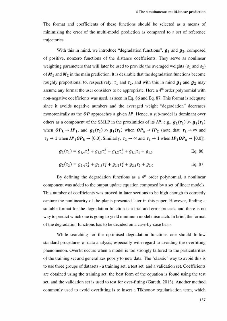
4 The simultaneous multi-linear prediction
137
The format and coefficients of these functions should be selected as a means of
minimising the error of the multi-model prediction as compared to a set of reference
trajectories.
With this in mind, we introduce “degradation functions”, 0� and 0 , composed
of positive, nonzero functions of the distance coefficients. They serve as nonlinear
weighting parameters that will later be used to provide the averaged weights ( � and �)
of � and in the main prediction. It is desirable that the degradation functions become
roughly proportional to, respectively, ¨� and ¨�, and with this in mind 0� and 0 may
assume any format the user considers to be appropriate. Here a 4th order polynomial with
non-negative coefficients was used, as seen in Eq. 86 and Eq. 87. This format is adequate
since it avoids negative numbers and the averaged weight “degradation” decreases
monotonically as the ±R approaches a given �R. Hence, a sub-model is dominant over
others as a component of the SMLP in the proximities of its �R, e.g., 0�k¨�m ≫ 0 k¨�m when ±R\ → �R�, and 0 k¨�m≫ 0�k¨�m when ±R\ → �R (note that ¨� → ∞ and
¨� → 1 when �R�±R\����������� → µ0,0·. Similarly, ¨� → ∞ and ¨� → 1 when �R ±R\����������� → µ0,0·).
0�k¨�m = A�,v¨�v + A�,W¨�W + A�,�¨�� + A�,�¨� + A�,B Eq. 86
0 k¨�m = A�,v¨�v + A�,W¨�W + A�,�¨�� + A�,�¨� + A�,B Eq. 87
By defining the degradation functions as a 4th order polynomial, a nonlinear
component was added to the output update equation composed by a set of linear models.
This number of coefficients was proved in later sections to be high enough to correctly
capture the nonlinearity of the plants presented later in this paper. However, finding a
suitable format for the degradation function is a trial and error process, and there is no
way to predict which one is going to yield minimum model mismatch. In brief, the format
of the degradation functions has to be decided on a case-by-case basis.
While searching for the optimised degradation functions one should follow
standard procedures of data analysis, especially with regard to avoiding the overfitting
phenomenon. Overfit occurs when a model is too strongly tailored to the particularities
of the training set and generalizes poorly to new data. The "classic" way to avoid this is
to use three groups of datasets - a training set, a test set, and a validation set. Coefficients
are obtained using the training set; the best form of the equation is found using the test
set, and the validation set is used to test for over-fitting (Gareth, 2013). Another method
commonly used to avoid overfitting is to insert a Tikhonov regularisation term, which
4 The simultaneous multi-linear prediction
138
aims at measuring the complexity of the function. The higher the complexity, the higher
the regularisation term will be (Tikhonov, 1963).
These standard procedures are well known, and the reader is strongly encouraged
to deploy them while applying the SMLP for engineering purposes. However, for the sake
of making the paper simpler and shorter, only a 2nd and a 4th order polynomials were
tested as degradation functions, and only a training dataset was used. Better results were
obtained for the 4th order polynomial, which is assumed to be optimal. Fig. 14 shows a
possible visual interpretation of functions 0� and 0 :
Fig. 14 – The “degradation functions”, 0� and 0 , are functions of the “distance coefficients” ©� and © .
The averaged weights for the arithmetic average between sub-models, ε� and ε�
are given by the proportion of � and in the sum of the degradation functions, as per
Eq. 88 and Eq. 89:
� = ?�kh�m?�kh�m|?pkhpm Eq. 88
� = ?pkhpm?�kh�m|?pkhpm Eq. 89
Note that � + � = 1. Finally, ε� and ε� are used in Eq. 90 to calculate the SMLP
output at k� + �m. The SMLP output, which may also be called “main output” or “multi-
model output” is normally the vector of CVs, but may sometimes contain other, non-
0 k© ‖�R ±R���������‖m
0�k©�‖�R�±R���������‖m
4 The simultaneous multi-linear prediction
139
controlled variables that we wish to monitor. It must contain exactly the same variables
as the sub-model outputs, i.e., dimk�\m = dimÔ�\��Ö = dimÔ�\� Ö.
µ�\|� − �\· = & �,(|�&�\|��� − �\��( �,(|�&�\|�� − �\� ((% Eq. 90
Note that the rate of change of w(|� is given by adding fractions ( �,(|� and �,(|�)
of the rates of change of �\|��� and �\|�� , and no discontinuity is introduced in the
prediction.
Now we will extend the multi-model approach to any number M� of linear sub-
models and any number MQ of CVs, i.e., ±R\ = >w�,(, … , w*�,(C, �R� =
>w�,a6� , … , w*�,a6�C ,… , �Rh� = >w�,a6#_ , … , w*�,a6#_C. As before, there will be as many
simultaneous sub-states and outputs as the number of sub-models, as shown in Eq. 91 and
Eq. 92:
\|��� = ���\�� + ���∆�\ + ��∆�\
⋮
\|��h� = ��h�\
�h� + ��h�∆�\ + �h�∆�\ Eq. 91
�\�� = ���\��
⋮
�\�h� = ��h�\
�h� Eq. 92
Eq. 93 may be used to obtain the distance coefficients,τj:
¨$ =∑ ∑ k�R«±R\�����������kb ∆Qb∗⁄#�bc�#_lc�∑ ‖�R�±R\�����������‖b ∆Qb∗⁄#�bc� , m = 1,… , M� Eq. 93
Note that the demominator of Eq. 93 contains the sum of the Euclidean norms of
the distances between the operating point ±R\ and identification point �R� k�R�±R\�����������m of
a particular sub-model �, for each CV ¯, where¯ = 1,… , MQ. The numerator,
however, contains the sum of the sum of Euclidean norms of the distances between ±R\
and �R« Ô�R«±R\�����������Ö for each CV ̄ , where¯ = 1,… , MQ, and each sub-model «, where n = 1,… , M�. The degradation function of sub-model � is given by Eq. 94:
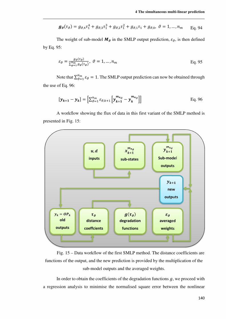
4 The simultaneous multi-linear prediction
140
0�k¨$m = A$,v¨�v + A$,W¨�W + A$,�¨�� + A$,�¨� + A$,B, m = 1,… , M� Eq. 94
The weight of sub-model � in the SMLP output prediction, $, is then defined
by Eq. 95:
$ = ?okhom∑ ?lÔhlÖ#_lc� , m = 1,… , M� Eq. 95
Note that∑ $*_$/� = 1. The SMLP output prediction can now be obtained through
the use of Eq. 96:
µ�\|� − �\· = >∑ $,(|� >�\|��ho − �\�hoC*_$/� C Eq. 96
A workflow showing the flux of data in this first variant of the SMLP method is
presented in Fig. 15:
Fig. 15 – Data workflow of the first SMLP method. The distance coefficients are
functions of the output, and the new prediction is provided by the multiplication of the
sub-model outputs and the averaged weights.
In order to obtain the coefficients of the degradation functions A, we proceed with
a regression analysis to minimise the normalised square error between the nonlinear
�\ = ±R\old
outputs
©�distance
coeffcients
0k©�mdegradation
functions
�\|��h�
Sub-model
outputs
\|��h�
sub-states
p�averaged
weights
�, �
inputs
�\|�
new
outputs
4 The simultaneous multi-linear prediction
141
model data (obtained from the commercial dynamic simulation package) and the SMLP,
using the same inputs, through the entire prediction horizon. We recommend using
several random trajectories and different starting points to properly identify the optimal
constants through a range of scenarios. For this first method, a SMLP system can be
defined as follows:
Definition 4.1.3.1 Simultaneous Multi-Linear Prediction system with
MIMO parametrisation (OP defined as the output vector). Let there be
a set of M� sub-models, where each sub-model � is defined by the state-
space matrices ��o, ��o, ��o and �o, a sub-state vector \�o and an
identification point �R$ = >w�,a6o , … , w*�,a6oC, where m = 1,… , M�, MQ is
the number of CVs and � is an arbitrary initial time. Let the sub-state vectors
for the next instant,\|��o , be provided by Eq. 91 and Eq. 92. Let the vector
of distance coefficients of sub-model �, ©� ∈ ℝ*_ , be yielded by the ratio
between ∑ �R«±R\�����������q/�,…,*_ and �R�±R\����������� normalised for each CV, as
defined in Eq. 93, where is the ±R\ operating point at time k, here defined
as ±R\ = >w�,(, … , w*�,(C, and w( is the main or multi-model output
prediction at time k. Let the degradation function of sub-model �, 0�k©�m, be defined by a set of non-negative coefficients A$,v, A$,W, A$,�, A$,� and A$,B. Let the weight of the sub-model � in the main output prediction for
each CV, $, be defined as the ratio between 0�k©�m and ∑ 0«Ô©«Ö*_q/� .
For such a system, �\|� can be obtained through the use of Eq. 96, and the
degradation function coefficients are obtained by solving the regression
analysis problem given by Eq. 97 for a number M@ of trajectories.
�¹M?o,r,?o,s,?o,p,?o,�,?o,t ∑ ∑ ∑ ÷>�u,Gh� − �u,G�hoC ë¹~A|���∗ − ��Vh∗ |.�ø�Lv$ Eq. 97
Where �h� is the training dataset provided by the dynamic simulator concerning
the trajectories being tested, m = 1,… , M�; � = 1,… , �; w = 1,… , M@, and M@ is the
number of reference trajectories that makes up the validation data set.
Hence, the regression analysis parameters assume values that reduce as much as
possible the prediction mismatch between the commercial dynamic simulation package
and the multi-model prediction. This provides us with a high degree of information about
the process, opening the “black box” of the commercial simulator and providing a proper
4 The simultaneous multi-linear prediction
142
basis for the EMOP analysis. The regression analysis problem of Eq. 97 is demanding
computationally for large MIMO systems and large datasets, so it cannot be done
continuously. If should be performed again every time changes occur to the plant,
alongside with sub-model identification, at least.
As a reference to measure the performance of the SMLP, let us define in a similar
way the linearisation error for a single sub-model �. The traditional single model
approach is the equivalent of setting the degradation function of sub-model � to $ =1, thus ignoring the other sub-models, yielding Eq. 98:
&)'*$xo/� =∑ ∑ Ô&�u,Gh� − �u,G�hm(ë¹~A|���∗ − ��Vh∗ |.�Ö�Lv Eq. 98
The formulation presented in this section for an output-tracking SMLP system
was defined with a view to avoiding the disadvantages of PWA systems presented in
section 2.4. The goal of the SMLP is enabling a good approximation of a nonlinear plant
using a small number of sub-models obtained at arbitrarily defined identification points,
while altogether avoiding the need of partitioning the state-space and the inherent
discontinuities thus introduced at the boundaries. Key to this formulation is the use of
“degradation functions”, that are defined to be continuous over the entire state-space, in
order to shift smoothly the weight of each sub-model in the SMLP output. The most
important step of the SMLP methodology is performing a regression analysis (Eq. 97) to
find adequate format and parameters for the degradation functions. Having an optimised
set of degradation functions results that, at any given point of the state-space, the SMLP
output will tend to follow the sub-models that perform best in that region, while ignoring
sub-models that perform poorly there, yielding a closer approximation to the nonlinear
plant through the state-space covered by the test and validation data. The more
comprehensive the data, the wider the range of states where the prediction is optimised.
An infinite number of states can be associated with a single OP. For this reason,
the degradation functions are defined over the OP space instead of over the space-state:
obtaining optimal coefficients for a degradation function defined over the space-state
would very likely be impossible given the issue of state multiplicity. Moreover, OP
concept is more intuitive, being widely applied in the chemical industry at large. In
industrial operations, operators refer to operating points, not states.
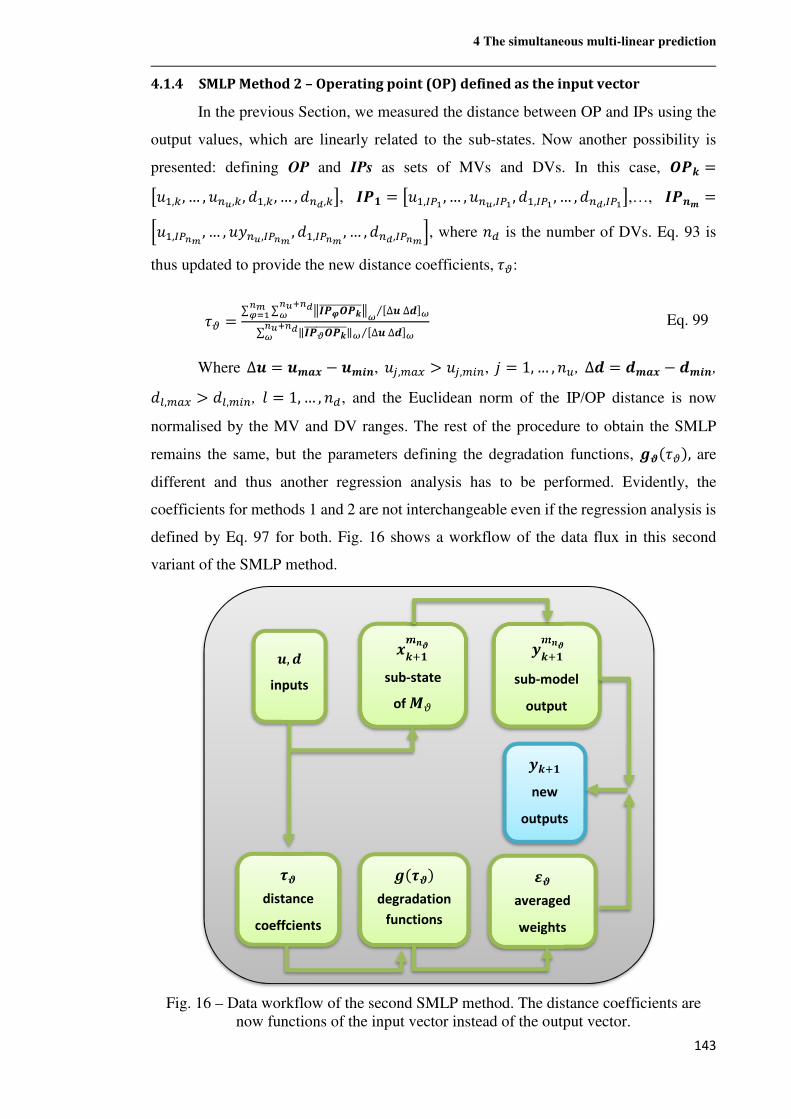
4 The simultaneous multi-linear prediction
143
4.1.4 SMLP Method 2 – Operating point (OP) defined as the input vector
In the previous Section, we measured the distance between OP and IPs using the
output values, which are linearly related to the sub-states. Now another possibility is
presented: defining OP and IPs as sets of MVs and DVs. In this case, ±R\ =&f�,(, … , f*�,(, ë�,(, … , ë*�,((, �R� = &f�,a6� , … , f*�,a6� , ë�,a6� , … , ë*�,a6�(,…, �Rh� =>f�,a6#_ , … , fw*�,a6#_ , ë�,a6#_ , … , ë*�,a6#_C, where M, is the number of DVs. Eq. 93 is
thus updated to provide the new distance coefficients,¨$:
¨$ =∑ ∑ k�R«±R\�����������kb µ∆�∆�·b⁄#�*#�b#_lc�∑ ‖�Ro±R\�����������‖b µ∆�∆�·b⁄#�*#�b Eq. 99
Where ∆� = ��� − ��Vh, fÝ,�?� > fÝ,�'*, à = 1, … , MP, ∆� = ��� − ��Vh,
ë),�?� > ë),�'*, F = 1, … , M,, and the Euclidean norm of the IP/OP distance is now
normalised by the MV and DV ranges. The rest of the procedure to obtain the SMLP
remains the same, but the parameters defining the degradation functions, 0�k¨$m, are
different and thus another regression analysis has to be performed. Evidently, the
coefficients for methods 1 and 2 are not interchangeable even if the regression analysis is
defined by Eq. 97 for both. Fig. 16 shows a workflow of the data flux in this second
variant of the SMLP method.
Fig. 16 – Data workflow of the second SMLP method. The distance coefficients are
now functions of the input vector instead of the output vector.
©�distance
coeffcients
0k©�mdegradation
functions
�\|��h�
sub-model
output
\|��h�
sub-state
of $
p�averaged
weights
�, �
inputs
�\|�new
outputs
4 The simultaneous multi-linear prediction
144
For this second method, a SMLP system can be defined as follows:
Definition 4.1.4.1 Simultaneous Multi-Linear Prediction system with
MIMO parametrisation (OP defined as the input vector). Let there be a
set of M� sub-models, where each sub-model � is defined by the state-
space matrices ��o, ��o, ��o and �o, a sub-state vector \�o and an
identification point �R$ = &f�,a6o , … , f*�,a6o , ë�,a6o , … , ë*�,a6o(, where m = 1,… , M�, MP is the number of MVs, M, is the number of DVs and � is
an arbitrary initial time. Let the sub-state vectors for the next instant,\|��o ,
be provided by Eq. 91 and Eq. 92. Let the vector of distance coefficients of
sub-model �, ©� ∈ ℝ*_ , be yielded by the ratio between ∑ �R«±R\�����������q/�,…,*_ and �R�±R\����������� normalised for each MV, as defined in
Eq. 99, where is the ±R\ operating point at time k, here defined as ±R\ =&f�,(, … , f*�,(, ë�,(, … , ë*�,((. Let the degradation function of sub-model
$, 0�k©�m, be defined by a set of non-negative coefficients A$,v, A$,W, A$,�, A$,� and A$,B. Let the weight of the sub-model � in the main output
prediction for each CV, $, be defined as the ratio between 0�k©�m and ∑ 0«Ô©«Ö*_q/� . For such a system, the main or multi-model output prediction
at time � + 1, �\|� can be obtained through the use of Eq. 96, and the
degradation function coefficients are obtained by solving the regression
analysis problem given by Eq. 97 for a number M@ of trajectories.
4.1.5 SMLP Method 3 – the SISO parametrisation
In previous Sections, the SMLP was based on the assumption that we can calculate
a single weight $ for each of the linear sub-model �, where m = 1,… , M�, which
dictates the overall contribution of model ϑ. In this case, the contribution to the prediction
calculation is, in relative terms, the same for all CVs and inputs. Let us return to the initial
example of Section 3.1, where the multi-linear prediction was provided by two sub-
models, � and , and we had two CVs, w� and w�. If, for instance, � > �, then sub-
model � is the main contributor for the prediction calculation of both w� and w�.
However, maybe at current OP sub-model � is adequate to calculate y�, while sub-
model is better suited to provide w�, or vice-versa. In this case, there may be some
accuracy gain by defining a different to each MV, for each sub-model. Let us carry out
a few changes in the multi-linear prediction to reflect this concept. Eq. 99 is modified to
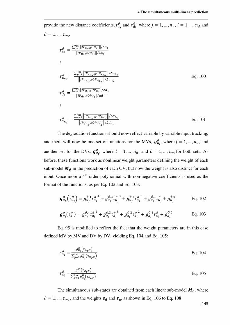
4 The simultaneous multi-linear prediction
145
provide the new distance coefficients, ¨P�$ and ¨,R$ , where à = 1,… , MP, F = 1,… , M, and m = 1,… , M�.
¨P�$ = ∑ ka6��,l56������������������k ∆P�⁄#_lc�ka6��,o56������������������k ∆P�⁄
⋮
¨P#�$ = ∑ ya6�#� ,l56�#���������������������y ∆P#�z#_lc�ya6�#� ,o56�#����������������������y ∆P#�z Eq. 100
¨,�$ = ∑ ka6��,l56�������������������k ∆,�⁄#_lc�ka6��,o56������������������k ∆,�⁄
⋮
¨,#�$ =∑ ya6�#� ,l56�#����������������������y ∆,#�z#_lc�ya6�#� ,o56�#����������������������y ∆,#�z Eq. 101
The degradation functions should now reflect variable by variable input tracking,
and there will now be one set of functions for the MVs, 0�Õ� , whereà = 1,… , MP, and
another set for the DVs, 0��� , where F = 1,… , M,, and m = 1,… , M�for both sets. As
before, these functions work as nonlinear weight parameters defining the weight of each
sub-model � in the prediction of each CV, but now the weight is also distinct for each
input. Once more a 4th order polynomial with non-negative coefficients is used as the
format of the functions, as per Eq. 102 and Eq. 103:
0�Õ� ÷¨P�$ ø = AP�$,v¨P�$ v + AP�$,W¨P�$ W + AP�$,�¨P�$ � + AP�$,�¨P�$ + AP�$,B Eq. 102
0��� Ô¨,R$ Ö = A,R$,v¨,R$ v + A,R$,W¨,R$ W + A,R$,�¨,R$ � + A,R$,�¨,R$ + A,R$,B Eq. 103
Eq. 95 is modified to reflect the fact that the weight parameters are in this case
defined MV by MV and DV by DV, yielding Eq. 104 and Eq. 105:
P�$ =?��o ÷h��,oø∑ ?��l ÷h��,lø#_lc� Eq. 104
,R$ = ?�Ro ÷h�R,oø∑ ?�Rl ÷h�R,lø#_lc� Eq. 105
The simultaneous sub-states are obtained from each linear sub-model �, where m = 1,… , M�, and the weights p� and p�, as shown in Eq. 106 to Eq. 108
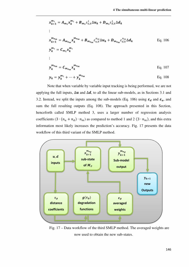
4 The simultaneous multi-linear prediction
146
\|��� = ���\�� + ��� P,(� ∆�\ + �� ,,(� ∆�\
⋮
\|��h� = ��h�\
�h� + ��h� P,(*_∆�\ + �h� ,,(*_∆�\ Eq. 106
�\�� = ���\��
⋮
�\�h� = ��h�\
�h� Eq. 107
�\ = �\�� +⋯+ �\�h� Eq. 108
Note that when variable by variable input tracking is being performed, we are not
applying the full inputs, ∆� and ∆�, to all the linear sub-models, as in Sections 3.1 and
3.2. Instead, we split the inputs among the sub-models (Eq. 106) using p� and p�, and
sum the full resulting outputs (Eq. 108). The approach presented in this Section,
henceforth called SMLP method 3, uses a larger number of regression analysis
coefficients (3 ∙ kMP + M,m ∙ M�) as compared to method 1 and 2 k3 ∙ M�m, and this extra
information most likely increases the prediction’s accuracy. Fig. 17 presents the data
workflow of this third variant of the SMLP method.
Fig. 17 – Data workflow of the third SMLP method. The averaged weights are
now used to obtain the new sub-states.
©�
distance
coeffcients
0k©�mdegradation
functions
�\|��h�
Sub-model
output
\|��h�
sub-state
of $
p�averaged
weights
�, �
inputs
Ë{|�new
Outputs
4 The simultaneous multi-linear prediction
147
A new regression analysis problem arises to obtain the coefficients of the
functions 0�Õ,�k¨$m and 0��,�k¨$m. As before, we wish to minimise the square error
between the nonlinear model and the SMLP, using a random trajectory, through the entire
prediction horizon.
For this third method, a SMLP system is defined as follows:
Definition 4.1.5.1 Simultaneous Multi-Linear Prediction system with
SISO parametrisation (OP defined as the input vector). Let there be a
set of M� sub-models, where each sub-model � is defined by the state-
space matrices ��o, ��o, ��o and �o, a sub-state vector \�o and an
identification point �R$ = &f�,a6o , … , f*�,a6o , ë�,a6o , … , ë*�,a6o(, where m = 1,… , M�, MP is the number of MVs, M, is the number of DVs and � is
an arbitrary initial time. Let ̈ P�$ be the distance coefficient of sub-model �
related to the manipulated variable à, and ¨,R$ be the distance coefficient of
sub-model � related to the disturbance variable F, where à = 1,… , MP, F =1,… , M, and m = 1,… , M�. Let ¨P�$ be yielded by the ratio between
∑ y2dP|,q�dP|�������������y*_q/� and y2dP|,$�dP|�������������y normalised for each MV, and ¨,R$ be
yielded by the ratio between ∑ k2d,R,q�d(,,R���������������k*_q/� and k2d,R,$�d,R�������������k
normalised for each DV, as defined in Eq. 100 and Eq. 101, where is the
±R\ operating point at time k, here defined as ±R\ =&f�,(, … , f*�,(, ë�,(, … , ë*�,((. Let the degradation functions of sub-model
� related respectively to fÝ and ë), 0�Õ� ÷¨P�$ ø and 0��� Ô¨,R$ Ö, be defined by
the sets of non-negative coefficients AP�$,v, AP�$,W, AP�$,�, AP�$,� and AP�$,B and A,R$,v,
A,R$,W, A,R$,�, A,R$,� and A,R$,B. Let the weights of the sub-model � in the main
output prediction for fÝ and ë), P�$ and ,R$ , be defined respectively as the
ratio between AP�$ ÷¨P�,$ø and ∑ AP�q ÷¨P�,qø*_q/� and the ratio between
A,R$ Ô¨,R,$Ö and ∑ A,Rq Ô¨,R,qÖ*_q/� . For such a system, the sub-state vectors
for the next instant,\|�$ , can be obtained through the use of Eq. 106 and
Eq. 107. The main or multi-model output prediction at time � + 1, �\|�, is
given by Eq. 108, and the coefficients of the degradation functions are
obtained by solving the regression analysis problem given by Eq. 109. This
4 The simultaneous multi-linear prediction
148
problem is defined for the variable by variable input tracking over a number
M@ of trajectories.
�¹M?��o,r,?��o,s,?��o,p,?��o,�,?��o,t?�Ro,r,?�Ro,s,?�Ro,p,?�Ro,�,?�Ro,t∑ ∑ ∑ Ô&�u,Gh� − �u,G�hm(ë¹~A|���∗ − ��Vh∗ |.�Ö�Lv$ Eq.
109
For Eq. 109, we have as beforeà = 1, … , MP, F = 1,… , M,, m = 1,… , M�, � =1, … , �; w = 1,… , M@. 4.1.6 The stability of an SMLP system
Concerning the stability of a SLMP system, the following theorem is valid:
Theorem 4.1.6.1 the stability of an SMLP system. An SMLP system is
Lyapunov stable if and only if composed only of stable sub-models.
Proof. An SMLP system consists of the sum of a finite number of dynamic
responses relative to each sub-model, each of which is multiplied by a non-
negative scalar, . If all sub-models are stable, the dynamic responses that
make up the SMLP are going to be bound, and it is self-evident that the sum
of a finite number of bounded dynamic responses is also bounded. The
SMLP cannot make any of the individual responses unbounded. For
instance, let us consider model state matrix ��� of sub-model �. From
Lyapunov (1892), for continuous-time state-space formulations, if a model
matrix ��� has eigenvalues Â$ with negative real parts, the system is BIBO
(Bounded-Input Bounded-Output) stable. We have from the theorem of
ESMM (Eigenvalues of a Scalar Multiple of a Matrix) that the eigenvalues
$Â$ of matrix & $���( will also have negative real parts since $ ∈ µ0,1·. For discrete-time formulations, a model is asymptotically (Schur) stable if
and only if all the eigenvalues of its state matrix � have a magnitude less
than one, i.e. lie inside the unit circle. Assuming that the sub-model � is
stable and thus |Â$| ∈ µ0,1·, it results in $Â$ ∈ µ0,1·, and therefore the
response remains BIBO stable.
Being Lyapunov Stable is a requirement for all flowsheets being evaluated
through the use of the EMOP index (Strutzel and Bogle, 2016).
4 The simultaneous multi-linear prediction
149
4.1.7 Reachability of an SMLP system
It is desirable to know if any given value for \�hm can be reached, i.e., if the system
Ô��� , ���Ö is completely reachable. Hence, let us focus on the problem, defined in Eq.
110, of determining a sequence of m incremental control actions transferring the sub-state
vector from \�hm = �,� to \|�
�hm = �, .
�, − ���� �,�ÇÈÈÈÈÉÈÈÈÈÊ���
= &��� ������ …����.����(ÇÈÈÈÈÈÈÈÈÉÈÈÈÈÈÈÈÈÊZ��
µ∆�\∆�\|�…∆�\|�.�·bÇÈÈÈÈÈÈÈÉÈÈÈÈÈÈÈÊ∆�!b
Eq. 110
This is equivalent to solving the linear system of Eq. 111 with respect to ∆u}:
Z�� ∆�!b = ��� Eq. 111
The matrix Z�� ∈ ℝ��,��∙h� is called the reachability matrix of the subsystem.
A solution ∆�! to Eq. 111 exists if and only if ��� ∈ ��ÔZ��Ö, where ��ÔZ��Ö is the
set of states that are reachable from the initial state �,�. According to the Rouché-Capelli
theorem, this is true if �~M�ÔZ�� ���Ö = �~M�ÔZ��Ö and hence the following well-
known theorem is valid:
Theorem the complete reachability of a system (Kalman et al., 1969). The
subsystem Ô��� , ���Ö is completely reachable if and only its reachability
matrix is full rank, i.e., the largest rank possible for a matrix of the same
dimensions
The full rank value is the lesser of the number of rows and columns and in this
case r~M�ÔZ��Ö = � ∙ MP, where m = 1,… , M�. A proof of the theorem is presented in
Kalman et al. (1969). Let us now approach the multi-model reachability problem. The
reachability matrices and the desired states of each sub-model can be concatenated
yielding Eq. 112, the multi-model version of the system of Eq. 111. Note that the solution
∆�! is the same as for Eq. 111.
� Z��⋮Z�h�
�ÇÈÉÈÊZ
∆�!% = � ���⋮��h�
�ÇÈÉÈÊ�
Eq. 112
4 The simultaneous multi-linear prediction
150
The theorem bellow is valid for SMLP systems:
Theorem 4.1.7.1 the complete reachability of an SMLP system. An SMLP
system is completely reachable if and only if composed solely of completely
reachable sub-models.
Proof. If an SMLP system is composed solely of completely reachable sub-
models, the reachability matrices of each sub-model �,Z��, have full
rank and the reachability matrix of the SMLP system, Z, also has full
rank. Since Z is the concatenation of the individual Z��, where m =1,… , M�, it results in �~M�kZm = �~M�ÔZ��Ö = � ∙ MP. Likewise, Z
will be rank deficient and the SMLP system will not be completely
reachable if one or more sub-systems do not have full rank.
A completely reachable SMLP will be able to achieve any output value in the
unrestricted control problem. In addition to that, it is shown in Hautus (1972) that
controllability is a weaker condition than reachability, and also that controllable systems
are stabilisable. Therefore, if an SMLP is completely reachable it is also controllable and
stabilisable.
4.1.8 Filtering sub-state changes
Due to the unavoidable presence of measurement noise and unmeasured
disturbances in industrial, closed-loop MPC applications, the control engineer should
implement a state-estimator, such as a Kalman Filter, for each sub-state of a SMLP
system. The usual tuning considerations on this subject apply (Gelb, 1974). Please note
that the regression analysis problems given by Eq. 97 and Eq. 109 are affected by the
state-estimator tuning, and thus re-identification of the degradation functions is necessary
if any of the estimators is changed. In this paper, state-estimators were not required since
it was assumed that no measurement noise and no unmeasured disturbances were present
in the case-studies.
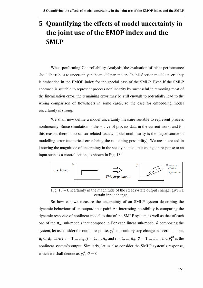
5 Quantifying the effects of model uncertainty in the joint use of the EMOP index and the SMLP
151
5 Quantifying the effects of model uncertainty in
the joint use of the EMOP index and the
SMLP
When performing Controllability Analysis, the evaluation of plant performance
should be robust to uncertainty in the model parameters. In this Section model uncertainty
is embedded in the EMOP Index for the special case of the SMLP. Even if the SMLP
approach is suitable to represent process nonlinearity by successful in removing most of
the linearisation error, the remaining error may be still enough to potentially lead to the
wrong comparison of flowsheets in some cases, so the case for embedding model
uncertainty is strong.
We shall now define a model uncertainty measure suitable to represent process
nonlinearity. Since simulation is the source of process data in the current work, and for
this reason, there is no sensor related issues, model nonlinearity is the major source of
modelling error (numerical error being the remaining possibility). We are interested in
knowing the magnitude of uncertainty in the steady-state output change in response to an
input such as a control action, as shown in Fig. 18:
Fig. 18 – Uncertainty in the magnitude of the steady-state output change, given a
certain input change.
So how can we measure the uncertainty of an SMLP system describing the
dynamic behaviour of an output/input pair? An interesting possibility is comparing the
dynamic response of nonlinear model to that of the SMLP system as well as that of each
one of the M� sub-models that compose it. For each linear sub-model m composing the
system, let us consider the output response, w'$, to a unitary step change in a certain input,
fÝ or ë', where ¹ = 1,… , MQ, à = 1,… , MP and F = 1,… , M,, m = 1,… , M�, and �Vh� is the
nonlinear system’s output. Similarly, let us also consider the SMLP system’s response,
which we shall denote as w'$, m = 0.
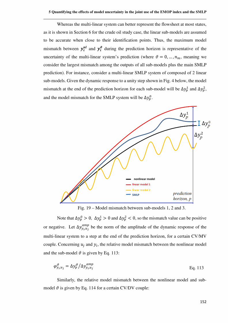
5 Quantifying the effects of model uncertainty in the joint use of the EMOP index and the SMLP
152
Whereas the multi-linear system can better represent the flowsheet at most states,
as it is shown in Section 6 for the crude oil study case, the linear sub-models are assumed
to be accurate when close to their identification points. Thus, the maximum model
mismatch between �Vh� and �V� during the prediction horizon is representative of the
uncertainty of the multi-linear system’s prediction (where m = 0,… , M�, meaning we
consider the largest mismatch among the outputs of all sub-models plus the main SMLP
prediction). For instance, consider a multi-linear SMLP system of composed of 2 linear
sub-models. Given the dynamic response to a unity step shown in Fig. 4 below, the model
mismatch at the end of the prediction horizon for each sub-model will be ∆wN� and ∆wN�,
and the model mismatch for the SMLP system will be ∆wNB.
Fig. 19 – Model mismatch between sub-models 1, 2 and 3.
Note that∆wNB > 0, ∆wN� > 0 and ∆wN� < 0, so the mismatch value can be positive
or negative. Let ∆wQx,P�?�N
be the norm of the amplitude of the dynamic response of the
multi-linear system to a step at the end of the prediction horizon, for a certain CV/MV
couple. Concerning fÝ and w', the relative model mismatch between the nonlinear model
and the sub-model m is given by Eq. 113:
nQx,P�$ = ∆wN$ ∆wQx,P�?�Nz Eq. 113
Similarly, the relative model mismatch between the nonlinear model and sub-
model m is given by Eq. 114 for a certain CV/DV couple:
SMLP
nonlinear model
5 Quantifying the effects of model uncertainty in the joint use of the EMOP index and the SMLP
153
nQx,,R$ = ∆wN$ ∆wQx,,R?�Nz Eq. 114
It is important to consider that if the output/input pair is weakly related
÷∆wQx,,R?�N < 0.01ornQx,P�$ < 0.01ø, the denominators in Eq. 113 and Eq. 114 will be small
and φ might become very large. In this case, this large uncertainty is meaningless and
unhelpful to the analysis, and thus the control engineer should ignore uncertainty for this
y/u or y/d pair by setting n = 0. It is important to notice that sub-models can be biased to
a direction, e.g., providing always smaller changes in output prediction than plant data,
consistently resulting in a negative model error. Or, alternatively, prediction error may be
randomly distributed for different steps. For this reason, �Qx,P�. and �Qx,P�| , respectively the
minimum negative relative mismatch and the maximum positive relative mismatch
between y¬ and u�, are defined Eq. 115 and Eq. 116:
�Qx,P�. = �¹M$/�,…,*_ �$ nQx,Px$ ,¹ = 1,… , MQ,à = 1,… , MP
Eq. 115
�Qx,P�| = �~u$/�,…,*_ê$ nQx,Px$ ,¹ = 1,… , MQ ,à = 1, … , MP
Eq. 116
where �$ = 1 and ê$ = 0 if nQ�,Px$ < 0, μj = 0 and ê$ = 1 if nQ�,Px$ > 0.
Parameters �Qx,P�. and �Qx,P�| may be understood as fractions of the nominal multi-model
response. Similarly, �Qx,,�. and �Qx,,�| are respectively the minimum negative and the
maximum positive relative model mismatch between w' and the DV ëÝ, as defined in Eq.
117 and Eq. 118:
�Qx,,R. = �¹M$/�,…,*� �$ nQx,,R$ ,¹ = 1,… , MQ,F = 1,… , M, Eq. 117
�Qx,,R| = �~u$/�,…,*�ê$ nQx,,R$ ,¹ = 1, … , MQ,F = 1,… , M, Eq. 118
The control engineer should test several operating points (OPs) throughout the
control zone and in the vicinity using different step amplitudes to obtain reliable sub-
models and to ensure that the magnitude of the resulting uncertainty parameter is
representative of nonlinearity effects. Let us define a set of matrices �P|, �P., �,| and �,.
in Eq. 119 to Eq. 122, which are going to store all model prediction error data from step
tests obtained for each possible coupling of y/u or y/d:
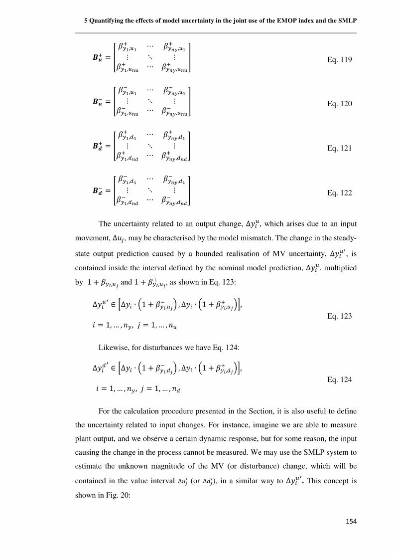
5 Quantifying the effects of model uncertainty in the joint use of the EMOP index and the SMLP
154
��| = � �Q�,P�| ⋯ �Q#�,P�|⋮ ⋱ ⋮�Q�,P#�| ⋯ �Q#�,P#�|� Eq. 119
��. = � �Q�,P�. ⋯ �Q#�,P�.⋮ ⋱ ⋮�Q�,P#�. ⋯ �Q#�,P#�.� Eq. 120
��| = � �Q�,,�| ⋯ �Q#�,,�|⋮ ⋱ ⋮�Q�,,#�| ⋯ �Q#�,,#�|� Eq. 121
��. = � �Q�,,�. ⋯ �Q#�,,�.⋮ ⋱ ⋮�Q�,,#�. ⋯ �Q#�,,#�.� Eq. 122
The uncertainty related to an output change, ∆w'P, which arises due to an input
movement, ∆fÝ, may be characterised by the model mismatch. The change in the steady-
state output prediction caused by a bounded realisation of MV uncertainty, ∆w'Py, is
contained inside the interval defined by the nominal model prediction, ∆w'P, multiplied
by 1 + �Q�,P�. and 1 + �Q�,P�| , as shown in Eq. 123:
∆w'Py ∈ >∆w' ∙ ÷1 + �Qx,P�. ø , ∆w' ∙ ÷1 + �Qx,P�| øC, ¹ = 1, … , MQ, à = 1,… , MP
Eq. 123
Likewise, for disturbances we have Eq. 124:
∆w',y ∈ >∆w' ∙ ÷1 + �Qx,,�. ø , ∆w' ∙ ÷1 + �Qx,,�| øC,
¹ = 1,… , MQ, à = 1,… , M, Eq. 124
For the calculation procedure presented in the Section, it is also useful to define
the uncertainty related to input changes. For instance, imagine we are able to measure
plant output, and we observe a certain dynamic response, but for some reason, the input
causing the change in the process cannot be measured. We may use the SMLP system to
estimate the unknown magnitude of the MV (or disturbance) change, which will be
contained in the value interval ∆fÝy (or ∆ëÝy), in a similar way to ∆w'Py. This concept is
shown in Fig. 20:
5 Quantifying the effects of model uncertainty in the joint use of the EMOP index and the SMLP
155
Fig. 20 – Uncertainty in the magnitude of an unknown input change, given a certain
output change.
Now this concept of uncertainty is clearly defined, and we have the understanding
that it describes input and output changes k∆f, ∆ë, ∆wm, not absolute values (f, ë, w).
Given this uncertainty definition, if a linear continuous-time state-space model is being
used, there is a relation of proportionality between ∆Qx��∆Qx� and∆P�
�∆P�
, and also between ∆Qx��∆Qx�
and ∆,��∆,�
. Due to model linearity, if we multiply an MV change, ∆fÝ, by any real number
contained in >1 + �Qx,P�. , 1 + �Qx,P�| C, the resulting output change will be contained inside
∆w'P. Similarly, multiplying a disturbance change, ∆ëÝ, by any real number contained in
>1 + �Qx,,�. , 1 + �Qx,,�| C, the resulting output change will be contained inside ∆w',. We use
this result to obtain Eq. 125 and Eq. 126, which are respectively the interval of control
action magnitude of the uncertain model, ∆fÝy, and the interval of disturbance magnitude
of the uncertain model, ∆ëÝy:
∆fÝy ∈ >∆fÝ ∙ ÷1 + �Qx,P�. ø , ∆fÝ ∙ ÷1 + �Qx,P�| øC, ¹ = 1, … , MQ, à = 1,… , MP
Eq. 125
∆ëÝy ∈ >∆ëÝ ∙ ÷1 + �Qx,,�. ø , ∆ë' ∙ ÷1 + �Qx,,�| øC, ¹ = 1,… , MQ, à = 1,… , M,
Eq. 126
Let us define two new variables, the uncertainty realisation parameters �Qx,P� and
�Qx,,�, which are real numbers that can assume any value inside the limits defined by,
respectively, >1 + �Q�,P�. , 1 + �Q�,P�| C and >1 + �Q�,,�. , 1 + �Q�,,�| C, as shown in Eq. 127 and Eq.
128:
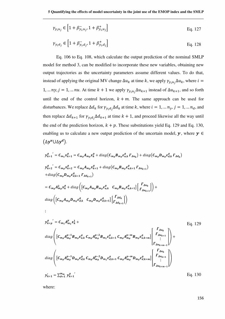
5 Quantifying the effects of model uncertainty in the joint use of the EMOP index and the SMLP
156
�QxP� ∈ >1 + �Qx,P�. , 1 + �Qx,P�| C Eq. 127
�Qx,� ∈ >1 + �Qx,,�. , 1 + �Qx,,�| C Eq. 128
Eq. 106 to Eq. 108, which calculate the output prediction of the nominal SMLP
model for method 3, can be modified to incorporate these new variables, obtaining new
output trajectories as the uncertainty parameters assume different values. To do that,
instead of applying the original MV change∆f( at time �, we apply �QxP�∆f(, where ¹ =1, …Mw, à = 1,…Mf. At time � + 1 we apply �QxP�∆f(|� instead of ∆f(|�, and so forth
until the end of the control horizon, � + �. The same approach can be used for
disturbances. We replace ∆ë( for �Qx,�∆ë( at time �, where ¹ = 1,…MQ, à = 1,…M,, and
then replace ∆ë(|� for �Qx,�∆ë(|� at time � + 1, and proceed likewise all the way until
the end of the prediction horizon, � + �. These substitutions yield Eq. 129 and Eq. 130,
enabling us to calculate a new output prediction of the uncertain model,�,, where �, ∈Ô∆��⋃∆��Ö. �\|�� y = ���\|�� = ������\� + ë¹~AÔ������p�,\� ���\Ö + ë¹~AÔ��� ��p�,\� ���\Ö
�\| � y = ���\| � = ������\|�� + ë¹~AÔ������p�,\|�� ���\*�Ö +ë¹~AÔ��� ��p�,\|�� ���\*�Ö
= ������ \� + ë¹~A I&���������p�,\� ������p�,\|�� ( # ���\���\*�$J +ë¹~A I&������ ��p�,\� ��� ��p�,\|�� ( # ���\���\*�$J
⋮
�\|Y� y = ������Y \� +
ë¹~A��&������Y.����p�,\� ������
Y. ���p�,\|�� ������Y.����p�,\|�� ( ��
�� ���\���\*�⋮���\*�@���
���� +
ë¹~A��&������Y.� ��p�,\� ������Y. ��p�,\|�� ������
Y.� ��p�,\|�� ( ���� ���\���\*�⋮���\*�@���
����
Eq. 129
�\|�y = ∑ �\|�����/� y
Eq. 130
where:
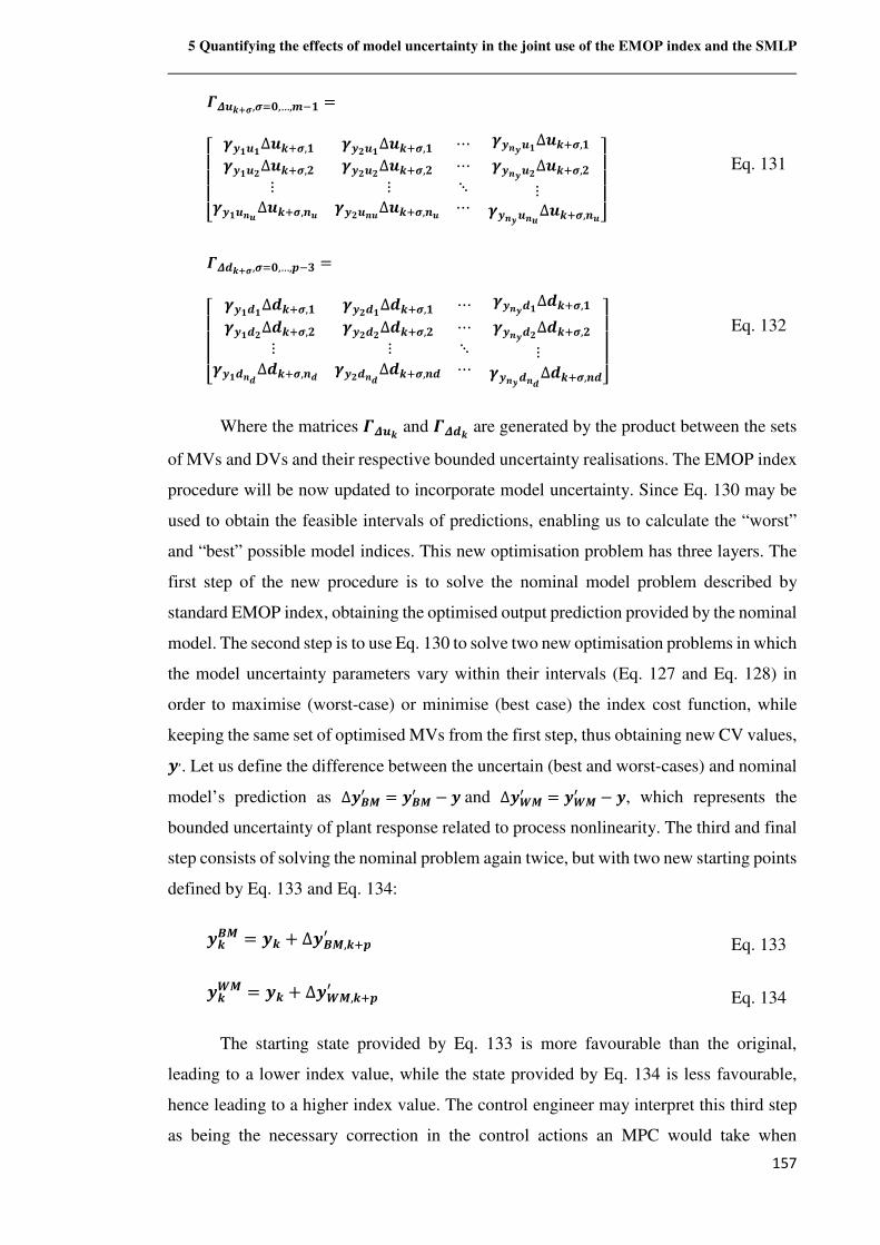
5 Quantifying the effects of model uncertainty in the joint use of the EMOP index and the SMLP
157
���\*¦,¦/¾,…,�.� =
����� �����∆�\|¦,� �� ��∆�\|¦,� ⋯���� ∆�\|¦, �� � ∆�\|¦, ⋯⋮ ⋮ ⋱
��h���∆�\|¦,���h�� ∆�\|¦, ⋮
����h�∆�\|¦,h� �� �h�∆�\|¦,h� ⋯��h��h�∆�\|¦,h������
Eq. 131
���\*¦,¦/¾,…,Y.' =
����� �����∆�\|¦,� �� ��∆�\|¦,� ⋯���� ∆�\|¦, �� � ∆�\|¦, ⋯⋮ ⋮ ⋱
��h���∆�\|¦,���h�� ∆�\|¦, ⋮
����h�∆�\|¦,h� �� �h�∆�\|¦,h� ⋯��h��h�∆�\|¦,h������ Eq. 132
Where the matrices ���\ and ���\ are generated by the product between the sets
of MVs and DVs and their respective bounded uncertainty realisations. The EMOP index
procedure will be now updated to incorporate model uncertainty. Since Eq. 130 may be
used to obtain the feasible intervals of predictions, enabling us to calculate the “worst”
and “best” possible model indices. This new optimisation problem has three layers. The
first step of the new procedure is to solve the nominal model problem described by
standard EMOP index, obtaining the optimised output prediction provided by the nominal
model. The second step is to use Eq. 130 to solve two new optimisation problems in which
the model uncertainty parameters vary within their intervals (Eq. 127 and Eq. 128) in
order to maximise (worst-case) or minimise (best case) the index cost function, while
keeping the same set of optimised MVs from the first step, thus obtaining new CV values,
�,. Let us define the difference between the uncertain (best and worst-cases) and nominal
model’s prediction as ∆��y = ��y − �and ∆�sy = �sy − �, which represents the
bounded uncertainty of plant response related to process nonlinearity. The third and final
step consists of solving the nominal problem again twice, but with two new starting points
defined by Eq. 133 and Eq. 134:
�\� = �\ + ∆��,\|Yy Eq. 133
�\s = �\ + ∆�s,\|Yy Eq. 134
The starting state provided by Eq. 133 is more favourable than the original,
leading to a lower index value, while the state provided by Eq. 134 is less favourable,
hence leading to a higher index value. The control engineer may interpret this third step
as being the necessary correction in the control actions an MPC would take when
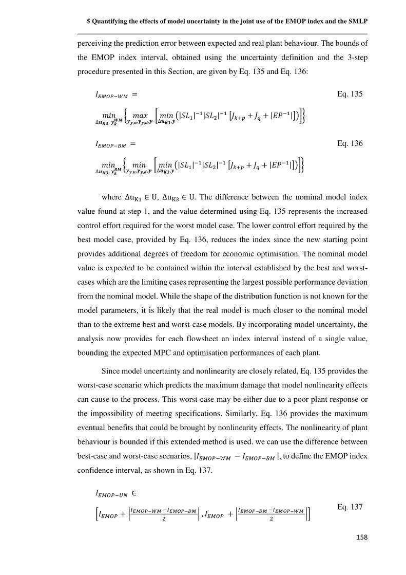
5 Quantifying the effects of model uncertainty in the joint use of the EMOP index and the SMLP
158
perceiving the prediction error between expected and real plant behaviour. The bounds of
the EMOP index interval, obtained using the uncertainty definition and the 3-step
procedure presented in this Section, are given by Eq. 135 and Eq. 136:
23456.:4 =
�¹M∆�!',�\s � �~u
��,�,��,�,�,#�¹M∆�!�,�
Ô|���|.�|���|.�&;(|N + ;> + |&d.�|(Ö$� Eq. 135
23456.74 =
�¹M∆�!',�\� � �¹M
��,�,��,�,�,#�¹M∆�!�,�
Ô|���|.�|���|.�&;(|N + ;> + |&d.�|(Ö$� Eq. 136
where ∆u}� ∈ U, ∆u}W ∈ U. The difference between the nominal model index
value found at step 1, and the value determined using Eq. 135 represents the increased
control effort required for the worst model case. The lower control effort required by the
best model case, provided by Eq. 136, reduces the index since the new starting point
provides additional degrees of freedom for economic optimisation. The nominal model
value is expected to be contained within the interval established by the best and worst-
cases which are the limiting cases representing the largest possible performance deviation
from the nominal model. While the shape of the distribution function is not known for the
model parameters, it is likely that the real model is much closer to the nominal model
than to the extreme best and worst-case models. By incorporating model uncertainty, the
analysis now provides for each flowsheet an index interval instead of a single value,
bounding the expected MPC and optimisation performances of each plant.
Since model uncertainty and nonlinearity are closely related, Eq. 135 provides the
worst-case scenario which predicts the maximum damage that model nonlinearity effects
can cause to the process. This worst-case may be either due to a poor plant response or
the impossibility of meeting specifications. Similarly, Eq. 136 provides the maximum
eventual benefits that could be brought by nonlinearity effects. The nonlinearity of plant
behaviour is bounded if this extended method is used. we can use the difference between
best-case and worst-case scenarios, |23456.:4 − 23456.74|, to define the EMOP index
confidence interval, as shown in Eq. 137.
23456.89 ∈
>23456 + �a����@��.a����@��� � , 23456 + �a����@��.a����@��
� �C Eq. 137
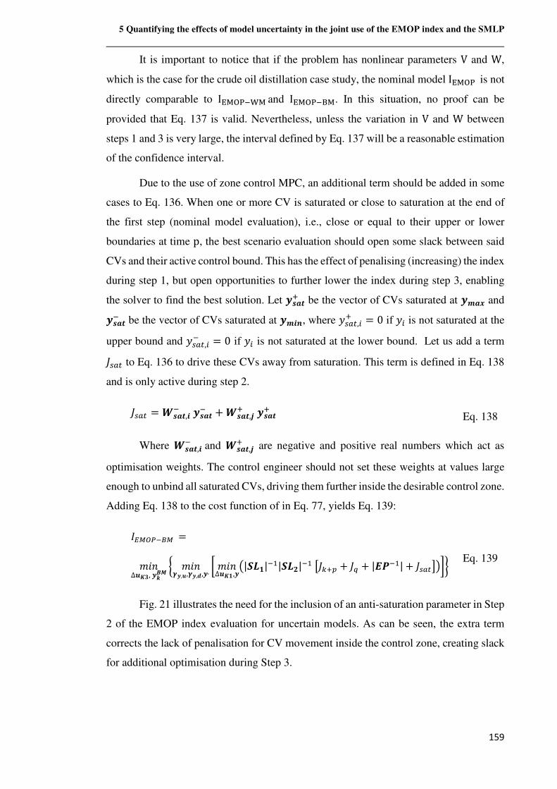
5 Quantifying the effects of model uncertainty in the joint use of the EMOP index and the SMLP
159
It is important to notice that if the problem has nonlinear parameters V and W,
which is the case for the crude oil distillation case study, the nominal model I ¡¢£ is not
directly comparable to I ¡¢£.¤¡and I ¡¢£.¥¡. In this situation, no proof can be
provided that Eq. 137 is valid. Nevertheless, unless the variation in V and W between
steps 1 and 3 is very large, the interval defined by Eq. 137 will be a reasonable estimation
of the confidence interval.
Due to the use of zone control MPC, an additional term should be added in some
cases to Eq. 136. When one or more CV is saturated or close to saturation at the end of
the first step (nominal model evaluation), i.e., close or equal to their upper or lower
boundaries at time p, the best scenario evaluation should open some slack between said
CVs and their active control bound. This has the effect of penalising (increasing) the index
during step 1, but open opportunities to further lower the index during step 3, enabling
the solver to find the best solution. Let �i�{| be the vector of CVs saturated at ��� and
�i�{. be the vector of CVs saturated at ��Vh, where w�?@,'| = 0 if w' is not saturated at the
upper bound and w�?@,'. = 0 if w' is not saturated at the lower bound. Let us add a term
;�?@ to Eq. 136 to drive these CVs away from saturation. This term is defined in Eq. 138
and is only active during step 2.
;�?@ = si�{,V. �i�{. +si�{,Õ
| �i�{| Eq. 138
Where si�{,V. and si�{,Õ
| are negative and positive real numbers which act as
optimisation weights. The control engineer should not set these weights at values large
enough to unbind all saturated CVs, driving them further inside the desirable control zone.
Adding Eq. 138 to the cost function of in Eq. 77, yields Eq. 139:
23456.74 =
�¹M∆�!',�\� � �¹M
��,�,��,�,�,#�¹M∆�!�,�
Ô|_`�|.�|_` |.�&;(|N + ;> + |cR.�|+ ;�?@(Ö$� Eq. 139
Fig. 21 illustrates the need for the inclusion of an anti-saturation parameter in Step
2 of the EMOP index evaluation for uncertain models. As can be seen, the extra term
corrects the lack of penalisation for CV movement inside the control zone, creating slack
for additional optimisation during Step 3.
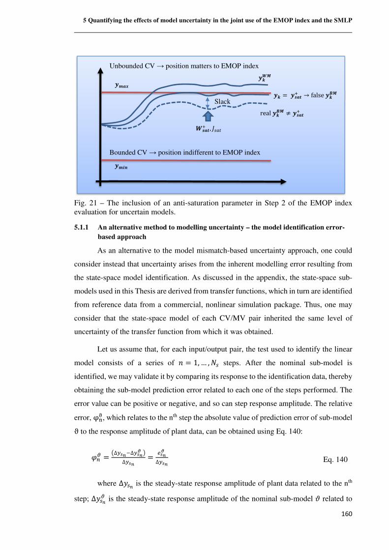
5 Quantifying the effects of model uncertainty in the joint use of the EMOP index and the SMLP
160
Fig. 21 – The inclusion of an anti-saturation parameter in Step 2 of the EMOP index evaluation for uncertain models.
5.1.1 An alternative method to modelling uncertainty – the model identification error-
based approach
As an alternative to the model mismatch-based uncertainty approach, one could
consider instead that uncertainty arises from the inherent modelling error resulting from
the state-space model identification. As discussed in the appendix, the state-space sub-
models used in this Thesis are derived from transfer functions, which in turn are identified
from reference data from a commercial, nonlinear simulation package. Thus, one may
consider that the state-space model of each CV/MV pair inherited the same level of
uncertainty of the transfer function from which it was obtained.
Let us assume that, for each input/output pair, the test used to identify the linear
model consists of a series of M = 1,… ,O� steps. After the nominal sub-model is
identified, we may validate it by comparing its response to the identification data, thereby
obtaining the sub-model prediction error related to each one of the steps performed. The
error value can be positive or negative, and so can step response amplitude. The relative
error, φýj , which relates to the nth step the absolute value of prediction error of sub-model
ϑ to the response amplitude of plant data, can be obtained using Eq. 140:
n*$ = Ô∆Q¦#.∆Q¦#o Ö∆Q¦# = L¦#o
∆Q¦# Eq. 140
where ∆w�# is the steady-state response amplitude of plant data related to the nth
step; ∆w�#$ is the steady-state response amplitude of the nominal sub-model m related to
�\ =�i�{| → false�\� real�\� ≠ �i�{|
�\s
Slack
Bounded CV → position indifferent to EMOP index
Unbounded CV → position matters to EMOP index
si�{| , ;�?@
��Vh
���
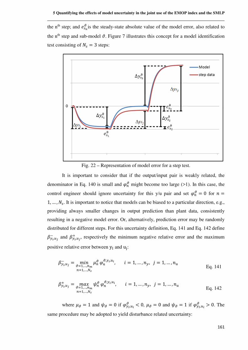
5 Quantifying the effects of model uncertainty in the joint use of the EMOP index and the SMLP
161
the nth step; and "�#$ is the steady-state absolute value of the model error, also related to
the nth step and sub-model m. Figure 7 illustrates this concept for a model identification
test consisting of O� = 3 steps:
Fig. 22 – Representation of model error for a step test.
It is important to consider that if the output/input pair is weakly related, the
denominator in Eq. 140 is small and n*$ might become too large (>1). In this case, the
control engineer should ignore uncertainty for this y/u pair and set n*$ = 0 for M =1, … , O�. It is important to notice that models can be biased to a particular direction, e.g.,
providing always smaller changes in output prediction than plant data, consistently
resulting in a negative model error. Or, alternatively, prediction error may be randomly
distributed for different steps. For this uncertainty definition, Eq. 141 and Eq. 142 define �Qx,P�. and �Qx,P�| , respectively the minimum negative relative error and the maximum
positive relative error between y� and u�:
�Qx,P�. = �¹M$/�,…,*_*/�,…,9¦
�*$ n*$,Qx,Px ,¹ = 1,… , MQ,à = 1,… , MP Eq. 141
�Qx,P�| = �~u$/�,…,*_*/�,…,9¦
ê*$ n*$,Qx,Px ,¹ = 1,… , MQ,à = 1,… , MP Eq. 142
where �$ = 1 and ê$ = 0 if nQ�,Px$ < 0, �$ = 0 and ê$ = 1 if nQ�,Px$ > 0. The
same procedure may be adopted to yield disturbance related uncertainty:
5 Quantifying the effects of model uncertainty in the joint use of the EMOP index and the SMLP
162
�Qx,,�. = �¹M$/�,…,*_*/�,…,9¦
�*$ n*$,Qx,Px ,¹ = 1, … , MQ,à = 1,… , M, Eq. 143
�Qx,,�| = �~u$/�,…,*_*/�,…,9¦
ê*$ n*$,Qx,Px ,¹ = 1,… , MQ,à = 1,… , M, Eq. 144
From this point, the procedure is similar as in the earlier Section. This approach
was used in Strutzel and Bogle (2016), but it was later replaced with the model mismatch
approach since the later was proved to capture the nonlinearity effects more efficiently.
Matrices ��,�. , ��,�| , ��,�. and ��,�| seemed to be undersized by the model identification
error approach presented in this Section.
This happens because nonlinearity can be better observed in the change of the
operating point from which model identification is performed, rather than in the steps
tests themselves. The step inputs cannot be large enough to reveal the whole model
uncertainty under penalty of destabilising the control system and even the dynamic
simulation itself.
6 Case of Study - EMOP Index for an Oil Distillation Process Unit
163
6 Case of Study - EMOP Index for an Oil
Distillation Process Unit
To demonstrate how the EMOP index may be applied to provide solutions to
industrial scale problems, three possible designs for a crude oil distillation plant shall be
presented. Also, a common set of controlled and manipulated variables for the MPC
control problem will be defined. As the index is related to the best possible solution for
this control problem, its value will indicate which plant can be better controlled by a well-
tuned MPC controller. The index will be evaluated for two different scenarios and four
distinct designs.
6.1 Describing the Control Problem
The models of the plants presented here were obtained through dynamic
simulation using Honeywell's UniSim® software. They have a very similar design, but
present key differences. These differences represent significant design decisions that the
project engineers have to make through the process of specifying the layout and
dimensions of a chemical plant. The distillation plants are rather simple and have a typical
configuration. The problem has 36 components, eight local PI controllers, 21 subsystems
and the column has 29 trays. This is considerably larger than the examples reported
above. The base case, or plant 1, can be seen Fig. 23.
The process simulated has a realistically drafted layout for a medium-sized crude
oil distillation process unit. The distillation column generates five different product
streams (Naphtha, Kerosene, Light Diesel, Heavy Diesel and Residue). The Kerosene,
Light Diesel, Heavy Diesel and Residue product streams are used to preheat the crude oil
feed from 25 °C to about 220 °C in two series of heat exchangers, yielding high energetic
efficiency. After the first series, the oil reaches an adequate temperature to enter the
desalter drum where salt is removed from the oil. After passing through the second series
of heat exchangers, the pre-heated oil enters a fired heater where its temperature is
increased to 320-380 °C. The hot crude is then fed to the distillation column where the
product streams are obtained. The cold light diesel and cold heavy diesel streams are
mixed to generate the “Pool Diesel” stream, whose properties will be used to evaluate the
cost index.
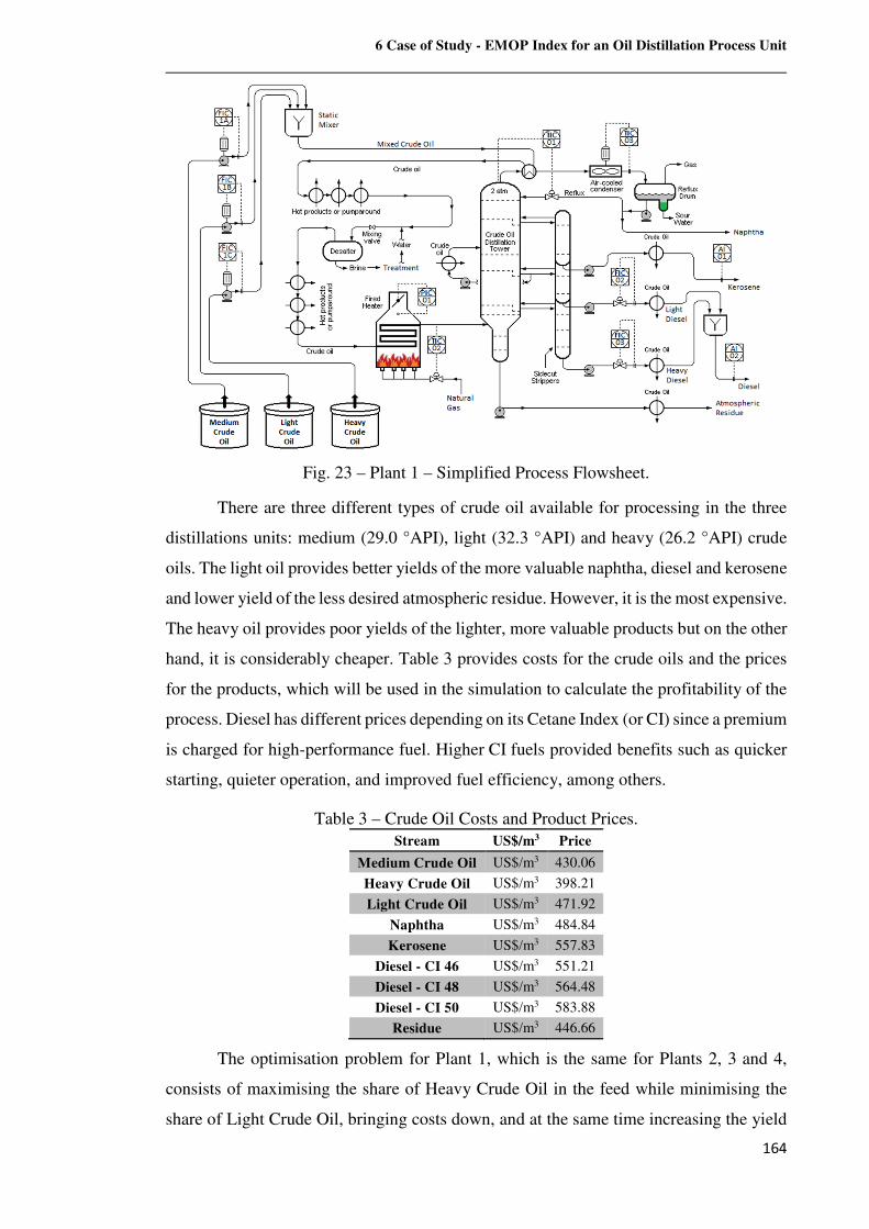
6 Case of Study - EMOP Index for an Oil Distillation Process Unit
164
Fig. 23 – Plant 1 – Simplified Process Flowsheet.
There are three different types of crude oil available for processing in the three
distillations units: medium (29.0 °API), light (32.3 °API) and heavy (26.2 °API) crude
oils. The light oil provides better yields of the more valuable naphtha, diesel and kerosene
and lower yield of the less desired atmospheric residue. However, it is the most expensive.
The heavy oil provides poor yields of the lighter, more valuable products but on the other
hand, it is considerably cheaper. Table 3 provides costs for the crude oils and the prices
for the products, which will be used in the simulation to calculate the profitability of the
process. Diesel has different prices depending on its Cetane Index (or CI) since a premium
is charged for high-performance fuel. Higher CI fuels provided benefits such as quicker
starting, quieter operation, and improved fuel efficiency, among others.
Table 3 – Crude Oil Costs and Product Prices.
Stream US$/m3 Price
Medium Crude Oil US$/m3 430.06
Heavy Crude Oil US$/m3 398.21
Light Crude Oil US$/m3 471.92
Naphtha US$/m3 484.84
Kerosene US$/m3 557.83
Diesel - CI 46 US$/m3 551.21
Diesel - CI 48 US$/m3 564.48
Diesel - CI 50 US$/m3 583.88
Residue US$/m3 446.66
The optimisation problem for Plant 1, which is the same for Plants 2, 3 and 4,
consists of maximising the share of Heavy Crude Oil in the feed while minimising the
share of Light Crude Oil, bringing costs down, and at the same time increasing the yield
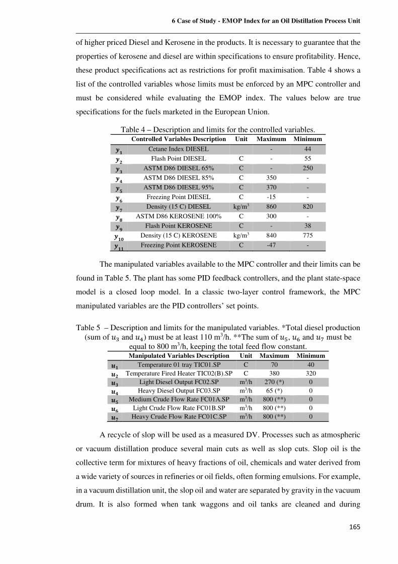
6 Case of Study - EMOP Index for an Oil Distillation Process Unit
165
of higher priced Diesel and Kerosene in the products. It is necessary to guarantee that the
properties of kerosene and diesel are within specifications to ensure profitability. Hence,
these product specifications act as restrictions for profit maximisation. Table 4 shows a
list of the controlled variables whose limits must be enforced by an MPC controller and
must be considered while evaluating the EMOP index. The values below are true
specifications for the fuels marketed in the European Union.
Table 4 – Description and limits for the controlled variables. Controlled Variables Description Unit Maximum Minimum
�� Cetane Index DIESEL - 44
� Flash Point DIESEL C - 55
�' ASTM D86 DIESEL 65% C - 250
�© ASTM D86 DIESEL 85% C 350 -
�ª ASTM D86 DIESEL 95% C 370 -
�« Freezing Point DIESEL C -15 -
�¬ Density (15 C) DIESEL kg/m3 860 820
� ASTM D86 KEROSENE 100% C 300 -
�\ Flash Point KEROSENE C - 38
��¾ Density (15 C) KEROSENE kg/m3 840 775
��� Freezing Point KEROSENE C -47 -
The manipulated variables available to the MPC controller and their limits can be
found in Table 5. The plant has some PID feedback controllers, and the plant state-space
model is a closed loop model. In a classic two-layer control framework, the MPC
manipulated variables are the PID controllers’ set points.
Table 5 – Description and limits for the manipulated variables. *Total diesel production (sum of fW and fv) must be at least 110 m3/h. **The sum of f�, f® and f¯ must be
equal to 800 m3/h, keeping the total feed flow constant. Manipulated Variables Description Unit Maximum Minimum
�� Temperature 01 tray TIC01.SP C 70 40
� Temperature Fired Heater TIC02(B).SP C 380 320
�' Light Diesel Output FC02.SP m3/h 270 (*) 0
�© Heavy Diesel Output FC03.SP m3/h 65 (*) 0
�ª Medium Crude Flow Rate FC01A.SP m3/h 800 (**) 0
�« Light Crude Flow Rate FC01B.SP m3/h 800 (**) 0
�¬ Heavy Crude Flow Rate FC01C.SP m3/h 800 (**) 0
A recycle of slop will be used as a measured DV. Processes such as atmospheric
or vacuum distillation produce several main cuts as well as slop cuts. Slop oil is the
collective term for mixtures of heavy fractions of oil, chemicals and water derived from
a wide variety of sources in refineries or oil fields, often forming emulsions. For example,
in a vacuum distillation unit, the slop oil and water are separated by gravity in the vacuum
drum. It is also formed when tank waggons and oil tanks are cleaned and during
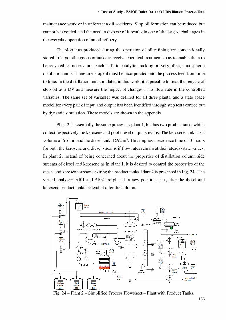
6 Case of Study - EMOP Index for an Oil Distillation Process Unit
166
maintenance work or in unforeseen oil accidents. Slop oil formation can be reduced but
cannot be avoided, and the need to dispose of it results in one of the largest challenges in
the everyday operation of an oil refinery.
The slop cuts produced during the operation of oil refining are conventionally
stored in large oil lagoons or tanks to receive chemical treatment so as to enable them to
be recycled to process units such as fluid catalytic cracking or, very often, atmospheric
distillation units. Therefore, slop oil must be incorporated into the process feed from time
to time. In the distillation unit simulated in this work, it is possible to treat the recycle of
slop oil as a DV and measure the impact of changes in its flow rate in the controlled
variables. The same set of variables was defined for all three plants, and a state space
model for every pair of input and output has been identified through step tests carried out
by dynamic simulation. These models are shown in the appendix.
Plant 2 is essentially the same process as plant 1, but has two product tanks which
collect respectively the kerosene and pool diesel output streams. The kerosene tank has a
volume of 616 m3 and the diesel tank, 1692 m3. This implies a residence time of 10 hours
for both the kerosene and diesel streams if flow rates remain at their steady-state values.
In plant 2, instead of being concerned about the properties of distillation column side
streams of diesel and kerosene as in plant 1, it is desired to control the properties of the
diesel and kerosene streams exiting the product tanks. Plant 2 is presented in Fig. 24. The
virtual analysers AI01 and AI02 are placed in new positions, i.e., after the diesel and
kerosene product tanks instead of after the column.
Fig. 24 – Plant 2 – Simplified Process Flowsheet – Plant with Product Tanks.
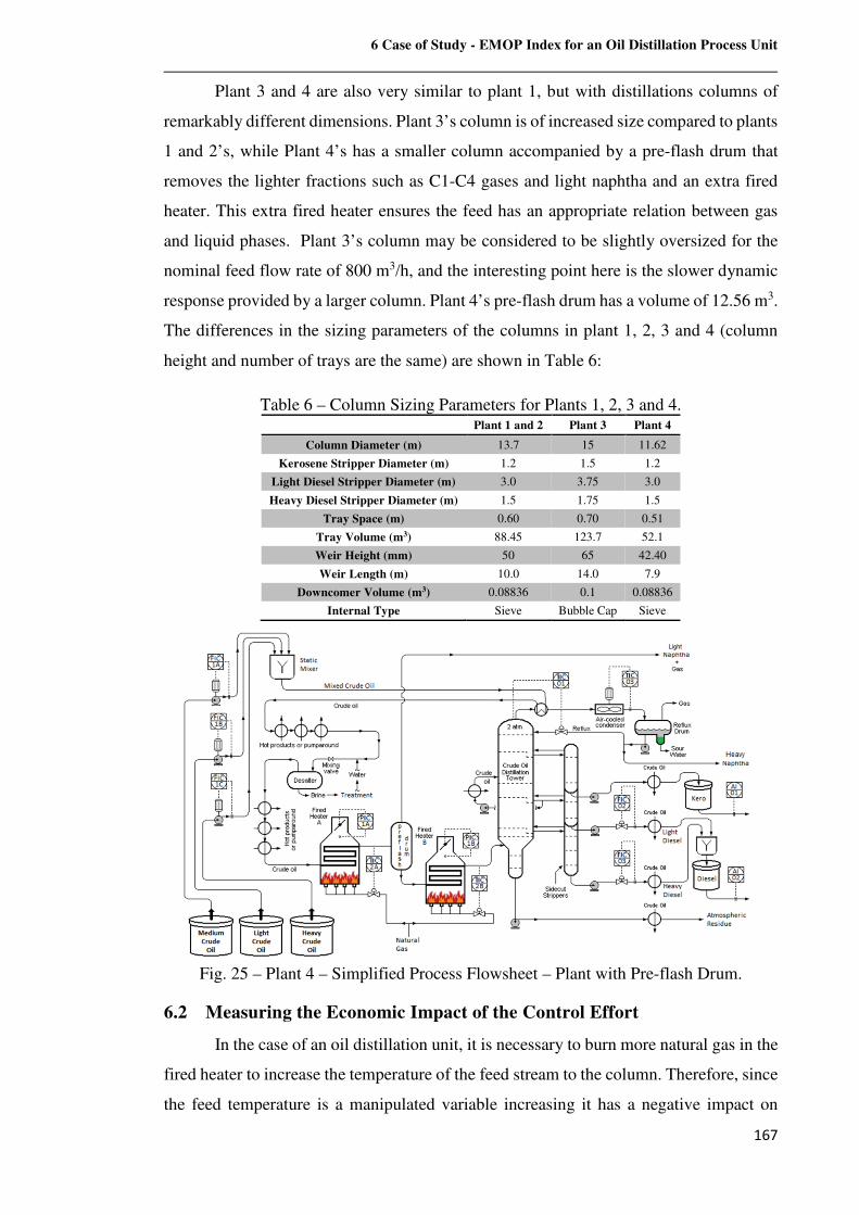
6 Case of Study - EMOP Index for an Oil Distillation Process Unit
167
Plant 3 and 4 are also very similar to plant 1, but with distillations columns of
remarkably different dimensions. Plant 3’s column is of increased size compared to plants
1 and 2’s, while Plant 4’s has a smaller column accompanied by a pre-flash drum that
removes the lighter fractions such as C1-C4 gases and light naphtha and an extra fired
heater. This extra fired heater ensures the feed has an appropriate relation between gas
and liquid phases. Plant 3’s column may be considered to be slightly oversized for the
nominal feed flow rate of 800 m3/h, and the interesting point here is the slower dynamic
response provided by a larger column. Plant 4’s pre-flash drum has a volume of 12.56 m3.
The differences in the sizing parameters of the columns in plant 1, 2, 3 and 4 (column
height and number of trays are the same) are shown in Table 6:
Table 6 – Column Sizing Parameters for Plants 1, 2, 3 and 4. Plant 1 and 2 Plant 3 Plant 4
Column Diameter (m) 13.7 15 11.62
Kerosene Stripper Diameter (m) 1.2 1.5 1.2
Light Diesel Stripper Diameter (m) 3.0 3.75 3.0
Heavy Diesel Stripper Diameter (m) 1.5 1.75 1.5
Tray Space (m) 0.60 0.70 0.51
Tray Volume (m3) 88.45 123.7 52.1
Weir Height (mm) 50 65 42.40
Weir Length (m) 10.0 14.0 7.9
Downcomer Volume (m3) 0.08836 0.1 0.08836
Internal Type Sieve Bubble Cap Sieve
Fig. 25 – Plant 4 – Simplified Process Flowsheet – Plant with Pre-flash Drum.
6.2 Measuring the Economic Impact of the Control Effort
In the case of an oil distillation unit, it is necessary to burn more natural gas in the
fired heater to increase the temperature of the feed stream to the column. Therefore, since
the feed temperature is a manipulated variable increasing it has a negative impact on
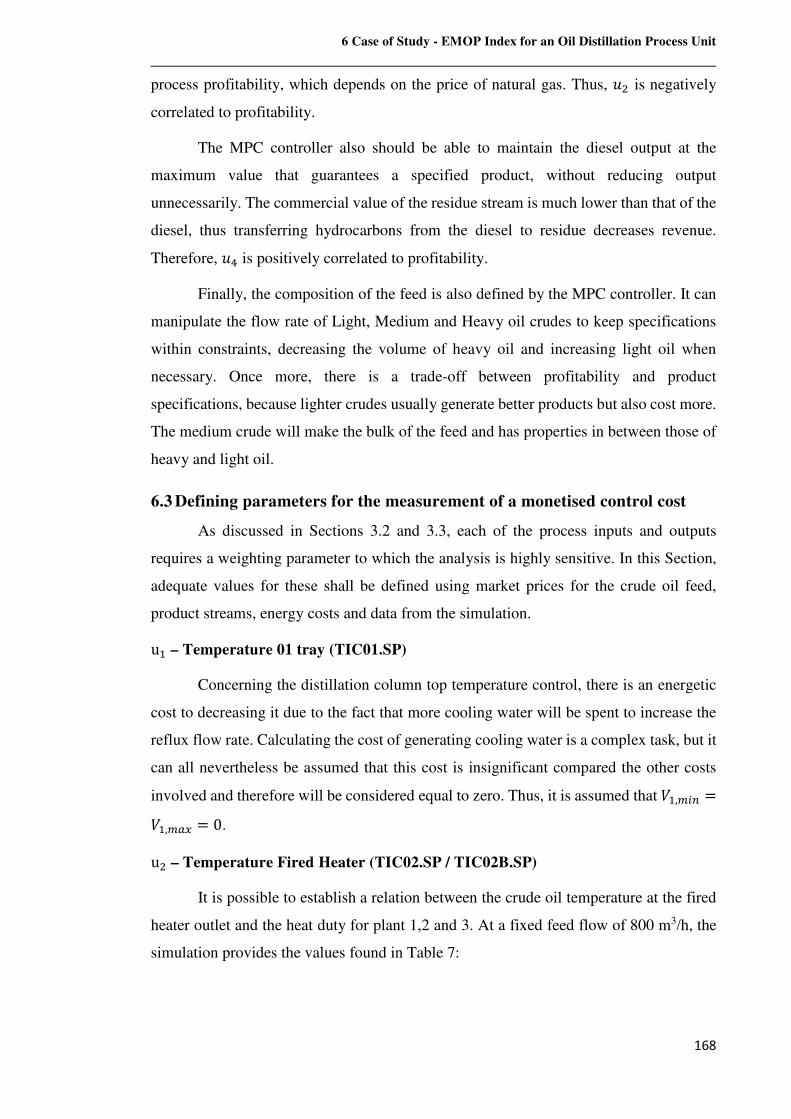
6 Case of Study - EMOP Index for an Oil Distillation Process Unit
168
process profitability, which depends on the price of natural gas. Thus, f� is negatively
correlated to profitability.
The MPC controller also should be able to maintain the diesel output at the
maximum value that guarantees a specified product, without reducing output
unnecessarily. The commercial value of the residue stream is much lower than that of the
diesel, thus transferring hydrocarbons from the diesel to residue decreases revenue.
Therefore, fv is positively correlated to profitability.
Finally, the composition of the feed is also defined by the MPC controller. It can
manipulate the flow rate of Light, Medium and Heavy oil crudes to keep specifications
within constraints, decreasing the volume of heavy oil and increasing light oil when
necessary. Once more, there is a trade-off between profitability and product
specifications, because lighter crudes usually generate better products but also cost more.
The medium crude will make the bulk of the feed and has properties in between those of
heavy and light oil.
6.3 Defining parameters for the measurement of a monetised control cost
As discussed in Sections 3.2 and 3.3, each of the process inputs and outputs
requires a weighting parameter to which the analysis is highly sensitive. In this Section,
adequate values for these shall be defined using market prices for the crude oil feed,
product streams, energy costs and data from the simulation.
u� – Temperature 01 tray (TIC01.SP)
Concerning the distillation column top temperature control, there is an energetic
cost to decreasing it due to the fact that more cooling water will be spent to increase the
reflux flow rate. Calculating the cost of generating cooling water is a complex task, but it
can all nevertheless be assumed that this cost is insignificant compared the other costs
involved and therefore will be considered equal to zero. Thus, it is assumed that -�,�'* =-�,�?� = 0.
u� – Temperature Fired Heater (TIC02.SP / TIC02B.SP)
It is possible to establish a relation between the crude oil temperature at the fired
heater outlet and the heat duty for plant 1,2 and 3. At a fixed feed flow of 800 m3/h, the
simulation provides the values found in Table 7:
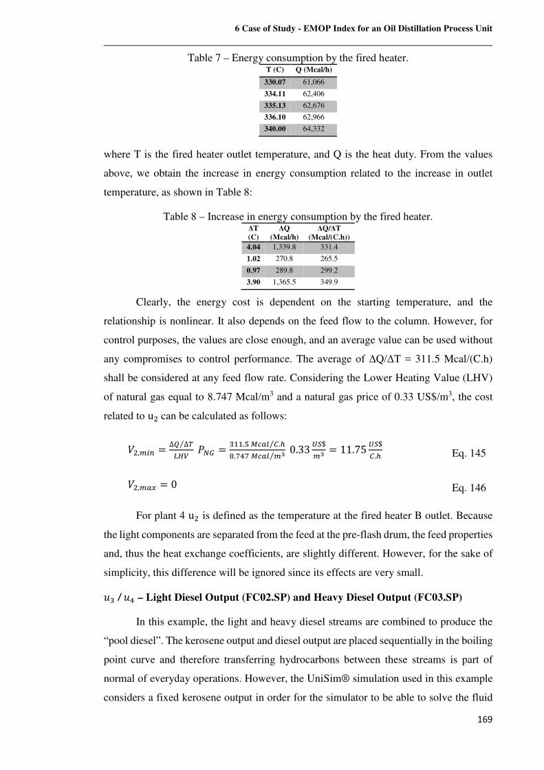
6 Case of Study - EMOP Index for an Oil Distillation Process Unit
169
Table 7 – Energy consumption by the fired heater. T (C) Q (Mcal/h)
330.07 61,066
334.11 62,406
335.13 62,676
336.10 62,966
340.00 64,332
where T is the fired heater outlet temperature, and Q is the heat duty. From the values
above, we obtain the increase in energy consumption related to the increase in outlet
temperature, as shown in Table 8:
Table 8 – Increase in energy consumption by the fired heater. ∆T (C)
∆Q (Mcal/h)
∆Q/∆T (Mcal/(C.h))
4.04 1,339.8 331.4
1.02 270.8 265.5
0.97 289.8 299.2
3.90 1,365.5 349.9
Clearly, the energy cost is dependent on the starting temperature, and the
relationship is nonlinear. It also depends on the feed flow to the column. However, for
control purposes, the values are close enough, and an average value can be used without
any compromises to control performance. The average of ∆Q/∆T = 311.5 Mcal/(C.h)
shall be considered at any feed flow rate. Considering the Lower Heating Value (LHV)
of natural gas equal to 8.747 Mcal/m3 and a natural gas price of 0.33 US$/m3, the cost
related to u�can be calculated as follows:
-�,�'* = ∆° ∆%⁄é±= d9² = W��.�4C?) <.³⁄´.¯v¯4C?) �s⁄ 0.33 8]$
�s = 11.75 8]$<.³ Eq. 145
-�,�?� = 0 Eq. 146
For plant 4 u� is defined as the temperature at the fired heater B outlet. Because
the light components are separated from the feed at the pre-flash drum, the feed properties
and, thus the heat exchange coefficients, are slightly different. However, for the sake of
simplicity, this difference will be ignored since its effects are very small.
fW / fv – Light Diesel Output (FC02.SP) and Heavy Diesel Output (FC03.SP)
In this example, the light and heavy diesel streams are combined to produce the
“pool diesel”. The kerosene output and diesel output are placed sequentially in the boiling
point curve and therefore transferring hydrocarbons between these streams is part of
normal of everyday operations. However, the UniSim® simulation used in this example
considers a fixed kerosene output in order for the simulator to be able to solve the fluid
6 Case of Study - EMOP Index for an Oil Distillation Process Unit
170
flow dynamic equations. However, there is a variable flux between the diesel output and
the residue output and thus the optimisation gain is defined as the price difference
between these streams:
-3,�~u = -4,�~u = dë¹"^"F − d�"^¹ëf" = 551.21 − 470.17 = 81.04 US$m3 Eq. 147
-3,�¹M = -4,�¹M = 0 Eq. 148
As discussed at the beginning of this Section, increasing heavy diesel output
reduces the residue output and thus increases profitability. In this case study the
separation between light and heavy diesel output has no commercial importance, but in
most refineries, these hydrocarbon streams have different destinations, such as being fed
to different hydrotreating or hydrocracking process units, and therefore they may have
different commercial values. These possibilities are not considered here.
5u – Medium Crude Oil Feed Flow Rate (FC01A.SP)
Given a set of flow rate values for each of the crude oils that compose the feed to
the distillation column, at any given time the average price of the oil processed is given
by:
d?JL = v��.®¸�¹|v¸®.¯®�º|v�¸.�¯�»�¹|�º|�» ¼½$
�s Eq. 149
The difference between average oil price and the medium crude will provide the
optimisation coefficient.
∆d�L,'P� = d�L,'P� − d?JL Eq. 150
Therefore, the following rule may be defined to obtain V�,�¬ý and V�,��¾:
if∆d�L,'P� > 0⟹ -�,�?� = 0,-�,�'* = ∆d�L,'P� Eq. 151
if∆d�L,'P� < 0⟹ -�,�?� = −∆d�L,'P�,-�,�'* = 0 Eq. 152
if∆d�L,'P� = 0⟹ -�,�?� = -�,�'* = 0 Eq. 153
In the third case, all feed is already entirely composed of medium crude and
average oil price doesn’t change with changes in u�.
6 Case of Study - EMOP Index for an Oil Distillation Process Unit
171
u®– Light Crude Oil Feed Flow Rate (FC01B.SP)
In a similar manner to the approach used for u�, the difference between average
oil price and the medium crude will provide the optimisation coefficient V®,�¬ý, and since
the light oil is the most expensive, the maximisation coefficient will always be zero.
-®,�'* = ∆d)'?³@ = d)'?³@ − d?JL Eq. 154
-®,�?� = 0 Eq. 155
u¯ – Heavy Crude Oil Feed Flow Rate (FC01C.SP)
In a similar manner to the approach used for 5u and 6u , the difference between an
average oil price and the medium crude will provide the optimisation coefficient V̄ ,��¾,
and since the light oil is the most expensive, the minimisation coefficient will always be
zero:
-̄ ,�?� = ∆d³L?JQ = d?JL−d³L?JQ Eq. 156
-̄ ,�'* = 0 Eq. 157
ë – Disturbance slop recycle
In the operation of oil refineries, slop streams require a complex and expensive
previous treatment to be able to be incorporated into the feed and reprocessed. In this case
study, however, this cost will be ignored. Such simplification will not change the EMOP
index problem because the slop recycle is a disturbance, and hence the MPC is not able
to fix anyway. Also, it is important to notice that the slop stream does not have a price
tag, meaning that it does not need to be purchased. Concerning the EMOP index, the
hydrocarbons recovered from slop are available for “free”. Therefore, they cause the
index to decrease in comparison with the first scenario once they replace crude oil in the
feed. At the same time, since slop is composed mostly of very heavy, difficult to process
oil cuts it diminishes the maximum quantity of cheap heavy oil that can be processed and
increases the energy consumption, and in its turn, these effects increase the index. This
discussion is to show that the relative values of the index are consequential to plant
assessment, not the absolute. The difference between the indexes of each plant is key to
evaluate performance.
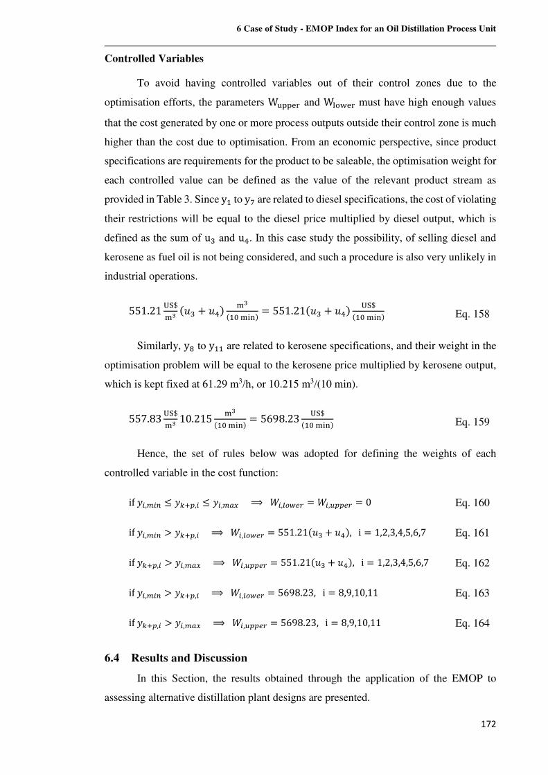
6 Case of Study - EMOP Index for an Oil Distillation Process Unit
172
Controlled Variables
To avoid having controlled variables out of their control zones due to the
optimisation efforts, the parameters W�22�À and W�ÁÂ�À must have high enough values
that the cost generated by one or more process outputs outside their control zone is much
higher than the cost due to optimisation. From an economic perspective, since product
specifications are requirements for the product to be saleable, the optimisation weight for
each controlled value can be defined as the value of the relevant product stream as
provided in Table 3. Since y� to y¯ are related to diesel specifications, the cost of violating
their restrictions will be equal to the diesel price multiplied by diesel output, which is
defined as the sum of uW and uv. In this case study the possibility, of selling diesel and
kerosene as fuel oil is not being considered, and such a procedure is also very unlikely in
industrial operations.
551.21 ¼½$�s kfW + fvm �s
k�B�¬ým = 551.21kfW + fvm ¼½$k�B�¬ým Eq. 158
Similarly, y´ to y�� are related to kerosene specifications, and their weight in the
optimisation problem will be equal to the kerosene price multiplied by kerosene output,
which is kept fixed at 61.29 m3/h, or 10.215 m3/(10 min).
557.83 ¼½$�s 10.215 �s
k�B�¬ým = 5698.23 ¼½$k�B�¬ým Eq. 159
Hence, the set of rules below was adopted for defining the weights of each
controlled variable in the cost function:
ifw',�'* ≤ w(|N,' ≤ w',�?� ⟹ �',)K�LH =�',PNNLH = 0 Eq. 160
ifw',�'* > w(|N,' ⟹ �',)K�LH = 551.21kfW + fvm,i = 1,2,3,4,5,6,7 Eq. 161
ifw(|N,' > w',�?� ⟹ �',PNNLH = 551.21kfW + fvm,i = 1,2,3,4,5,6,7 Eq. 162
ifw',�'* > w(|N,' ⟹ �',)K�LH = 5698.23,i = 8,9,10,11 Eq. 163
ifw(|N,' > w',�?� ⟹ �',PNNLH = 5698.23,i = 8,9,10,11 Eq. 164
6.4 Results and Discussion
In this Section, the results obtained through the application of the EMOP to
assessing alternative distillation plant designs are presented.
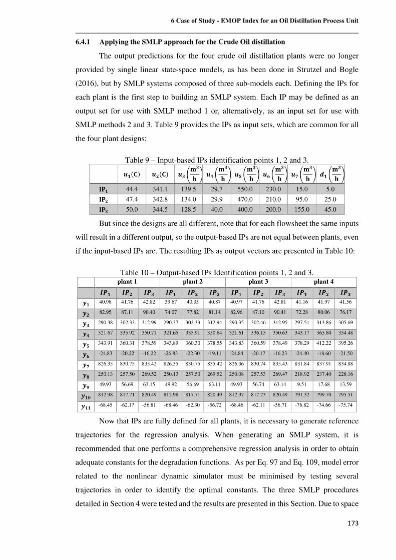
6 Case of Study - EMOP Index for an Oil Distillation Process Unit
173
6.4.1 Applying the SMLP approach for the Crude Oil distillation
The output predictions for the four crude oil distillation plants were no longer
provided by single linear state-space models, as has been done in Strutzel and Bogle
(2016), but by SMLP systems composed of three sub-models each. Defining the IPs for
each plant is the first step to building an SMLP system. Each IP may be defined as an
output set for use with SMLP method 1 or, alternatively, as an input set for use with
SMLP methods 2 and 3. Table 9 provides the IPs as input sets, which are common for all
the four plant designs:
Table 9 – Input-based IPs identification points 1, 2 and 3.
��kÅm � kÅm �' I4'Æ J �© I4'Æ J �ª I4'Æ J �« I4'Æ J �¬ I4'Æ J �� I4'Æ J3Ç� 44.4 341.1 139.5 29.7 550.0 230.0 15.0 5.0 3Ç 47.4 342.8 134.0 29.9 470.0 210.0 95.0 25.0 3Ç' 50.0 344.5 128.5 40.0 400.0 200.0 155.0 45.0
But since the designs are all different, note that for each flowsheet the same inputs
will result in a different output, so the output-based IPs are not equal between plants, even
if the input-based IPs are. The resulting IPs as output vectors are presented in Table 10:
Table 10 – Output-based IPs Identification points 1, 2 and 3. plant 1 plant 2 plant 3 plant 4
�R� �R �R' �R� �R �R' �R� �R �R' �R� �R �R'
�� 40.98 41.76 42.82 39.67 40.35 40.87 40.97 41.76 42.81 41.16 41.97 41.56
� 82.95 87.11 90.40 74.07 77.82 81.14 82.96 87.10 90.41 72.28 80.06 76.17
�' 290.38 302.33 312.99 290.37 302.33 312.94 290.35 302.46 312.95 297.51 313.86 305.69
�© 321.67 335.92 350.71 321.65 335.91 350.64 321.61 336.15 350.63 343.17 365.80 354.48
�ª 343.91 360.31 378.59 343.89 360.30 378.55 343.83 360.59 378.49 378.29 412.22 395.26
�« -24.83 -20.22 -16.22 -26.83 -22.30 -19.11 -24.84 -20.17 -16.23 -24.40 -18.60 -21.50
�¬ 826.35 830.75 835.42 826.35 830.75 835.42 826.36 830.74 835.43 831.84 837.91 834.88
� 250.13 257.50 269.52 250.13 257.50 269.52 250.08 257.53 269.47 218.92 237.40 228.16
�\ 49.93 56.69 63.15 49.92 56.69 63.11 49.93 56.74 63.14 9.51 17.68 13.59
��¾ 812.98 817.71 820.49 812.98 817.71 820.49 812.97 817.73 820.49 791.32 799.70 795.51
��� -68.45 -62.17 -56.81 -68.46 -62.30 -56.72 -68.46 -62.11 -56.71 -76.82 -74.66 -75.74
Now that IPs are fully defined for all plants, it is necessary to generate reference
trajectories for the regression analysis. When generating an SMLP system, it is
recommended that one performs a comprehensive regression analysis in order to obtain
adequate constants for the degradation functions. As per Eq. 97 and Eq. 109, model error
related to the nonlinear dynamic simulator must be minimised by testing several
trajectories in order to identify the optimal constants. The three SMLP procedures
detailed in Section 4 were tested and the results are presented in this Section. Due to space
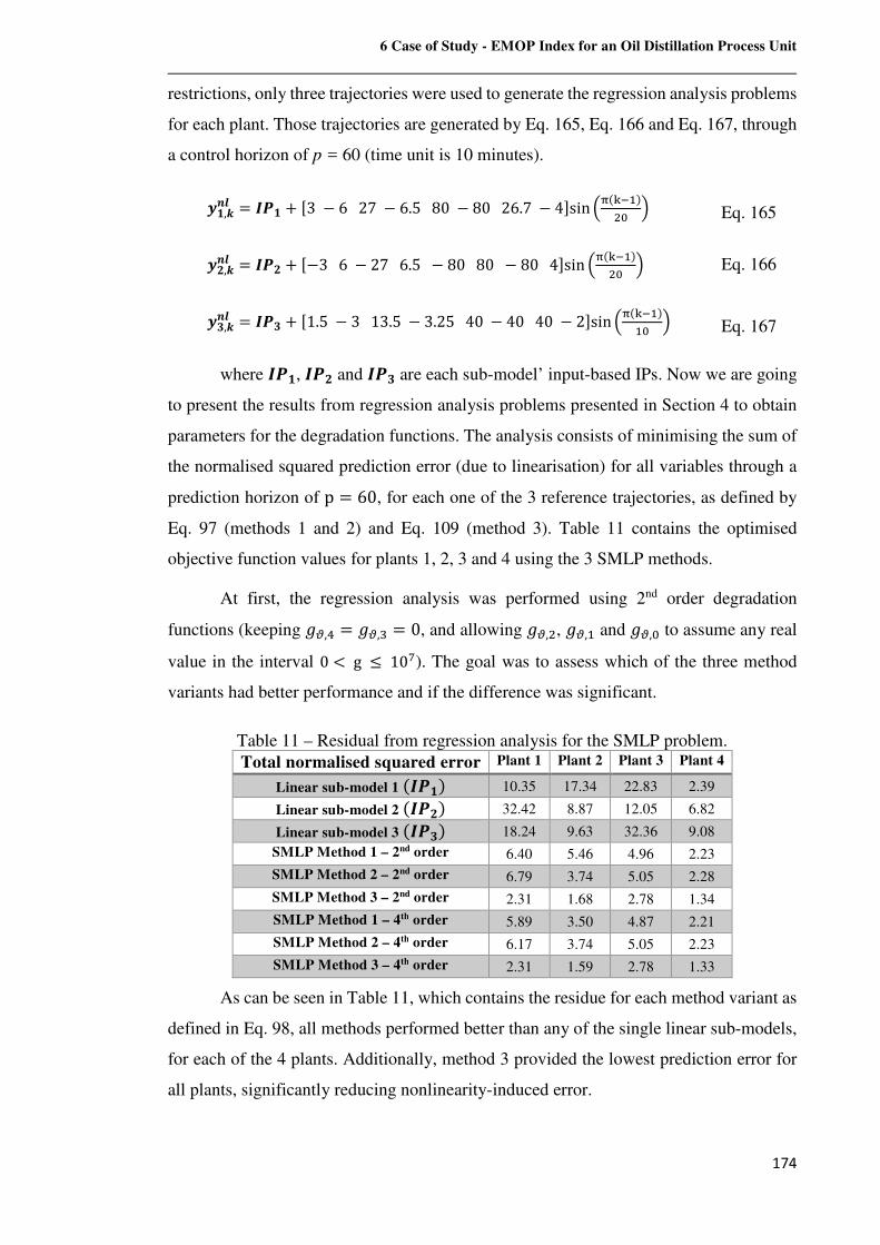
6 Case of Study - EMOP Index for an Oil Distillation Process Unit
174
restrictions, only three trajectories were used to generate the regression analysis problems
for each plant. Those trajectories are generated by Eq. 165, Eq. 166 and Eq. 167, through
a control horizon of p = 60 (time unit is 10 minutes).
��,\h� = �R� + µ3 − 627 − 6.580 − 8026.7 − 4·sin ÷Èk1.�m�B ø Eq. 165
� ,\h� = �R + µ−36 − 276.5 − 8080 − 804·sin ÷Èk1.�m�B ø Eq. 166
�',\h� = �R' + µ1.5 − 313.5 − 3.2540 − 4040 − 2·sin ÷Èk1.�m�B ø Eq. 167
where �R�, �R and �R' are each sub-model’ input-based IPs. Now we are going
to present the results from regression analysis problems presented in Section 4 to obtain
parameters for the degradation functions. The analysis consists of minimising the sum of
the normalised squared prediction error (due to linearisation) for all variables through a
prediction horizon of p = 60, for each one of the 3 reference trajectories, as defined by
Eq. 97 (methods 1 and 2) and Eq. 109 (method 3). Table 11 contains the optimised
objective function values for plants 1, 2, 3 and 4 using the 3 SMLP methods.
At first, the regression analysis was performed using 2nd order degradation
functions (keeping A$,v = A$,W = 0, and allowing A$,�, A$,� and A$,B to assume any real
value in the interval 0 < g ≤ 10¯). The goal was to assess which of the three method
variants had better performance and if the difference was significant.
Table 11 – Residual from regression analysis for the SMLP problem.
Total normalised squared error Plant 1 Plant 2 Plant 3 Plant 4
Linear sub-model 1 k�R�m 10.35 17.34 22.83 2.39
Linear sub-model 2 k�R m 32.42 8.87 12.05 6.82
Linear sub-model 3 k�R'm 18.24 9.63 32.36 9.08
SMLP Method 1 – 2nd order 6.40 5.46 4.96 2.23
SMLP Method 2 – 2nd order 6.79 3.74 5.05 2.28
SMLP Method 3 – 2nd order 2.31 1.68 2.78 1.34
SMLP Method 1 – 4th order 5.89 3.50 4.87 2.21
SMLP Method 2 – 4th order 6.17 3.74 5.05 2.23
SMLP Method 3 – 4th order 2.31 1.59 2.78 1.33
As can be seen in Table 11, which contains the residue for each method variant as
defined in Eq. 98, all methods performed better than any of the single linear sub-models,
for each of the 4 plants. Additionally, method 3 provided the lowest prediction error for
all plants, significantly reducing nonlinearity-induced error.
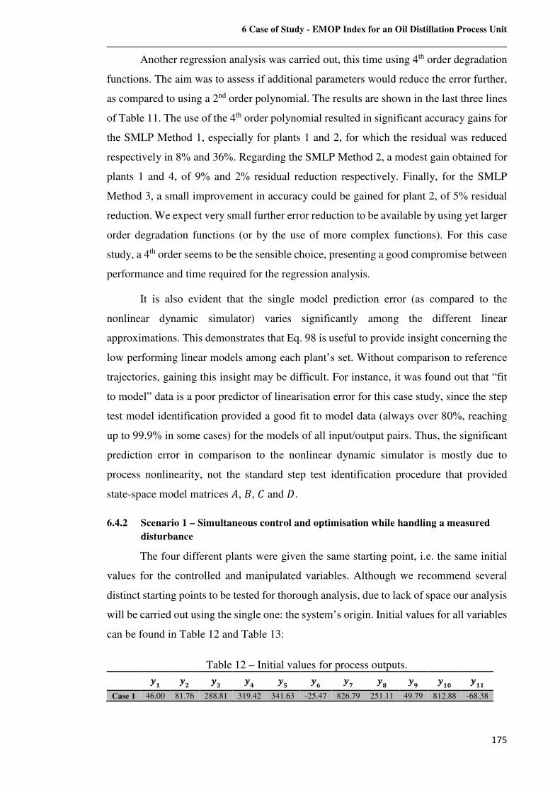
6 Case of Study - EMOP Index for an Oil Distillation Process Unit
175
Another regression analysis was carried out, this time using 4th order degradation
functions. The aim was to assess if additional parameters would reduce the error further,
as compared to using a 2nd order polynomial. The results are shown in the last three lines
of Table 11. The use of the 4th order polynomial resulted in significant accuracy gains for
the SMLP Method 1, especially for plants 1 and 2, for which the residual was reduced
respectively in 8% and 36%. Regarding the SMLP Method 2, a modest gain obtained for
plants 1 and 4, of 9% and 2% residual reduction respectively. Finally, for the SMLP
Method 3, a small improvement in accuracy could be gained for plant 2, of 5% residual
reduction. We expect very small further error reduction to be available by using yet larger
order degradation functions (or by the use of more complex functions). For this case
study, a 4th order seems to be the sensible choice, presenting a good compromise between
performance and time required for the regression analysis.
It is also evident that the single model prediction error (as compared to the
nonlinear dynamic simulator) varies significantly among the different linear
approximations. This demonstrates that Eq. 98 is useful to provide insight concerning the
low performing linear models among each plant’s set. Without comparison to reference
trajectories, gaining this insight may be difficult. For instance, it was found out that “fit
to model” data is a poor predictor of linearisation error for this case study, since the step
test model identification provided a good fit to model data (always over 80%, reaching
up to 99.9% in some cases) for the models of all input/output pairs. Thus, the significant
prediction error in comparison to the nonlinear dynamic simulator is mostly due to
process nonlinearity, not the standard step test identification procedure that provided
state-space model matrices �, �, Ê and �.
6.4.2 Scenario 1 – Simultaneous control and optimisation while handling a measured
disturbance
The four different plants were given the same starting point, i.e. the same initial
values for the controlled and manipulated variables. Although we recommend several
distinct starting points to be tested for thorough analysis, due to lack of space our analysis
will be carried out using the single one: the system’s origin. Initial values for all variables
can be found in Table 12 and Table 13:
Table 12 – Initial values for process outputs. �� � �' �© �ª �« �¬ � �\ ��¾ ���
Case 1 46.00 81.76 288.81 319.42 341.63 -25.47 826.79 251.11 49.79 812.88 -68.38
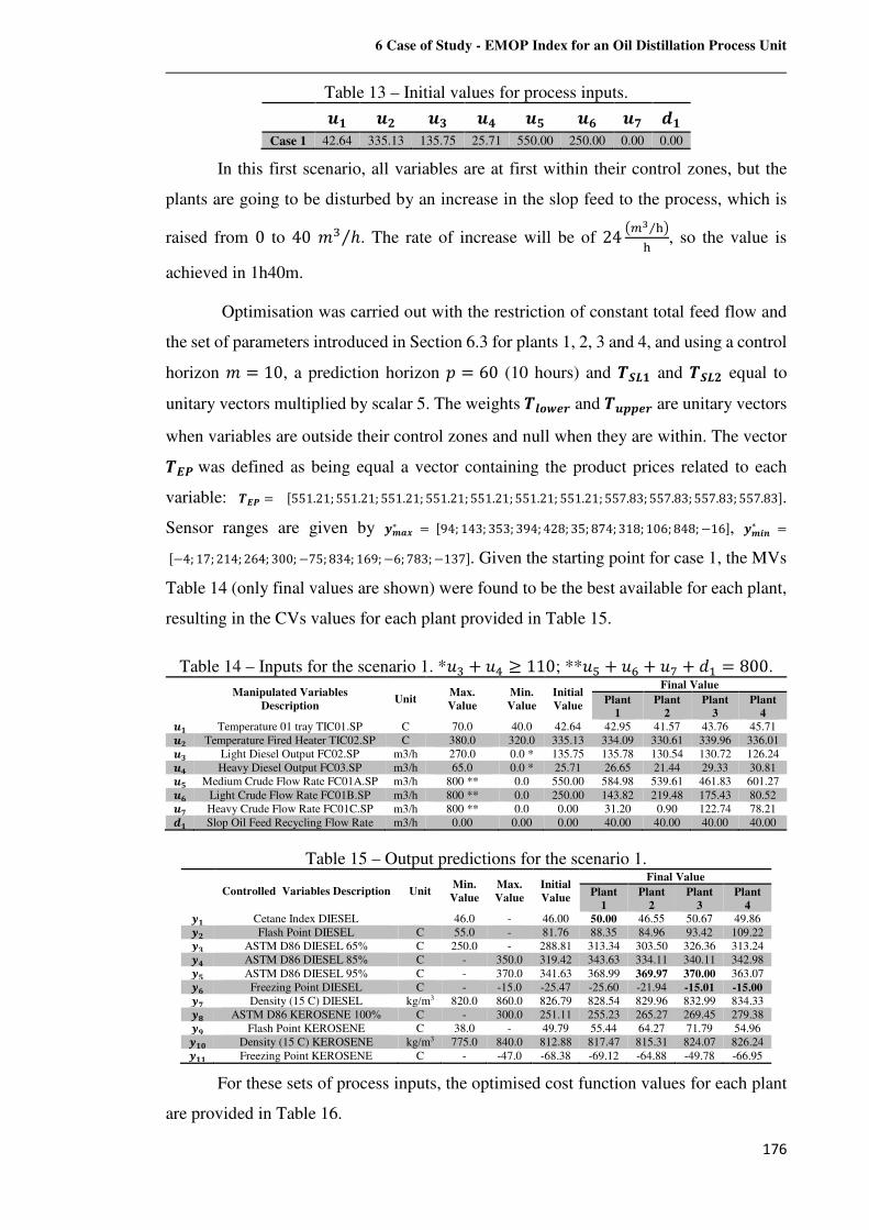
6 Case of Study - EMOP Index for an Oil Distillation Process Unit
176
Table 13 – Initial values for process inputs. �� � �' �© �ª �« �¬ ��
Case 1 42.64 335.13 135.75 25.71 550.00 250.00 0.00 0.00
In this first scenario, all variables are at first within their control zones, but the
plants are going to be disturbed by an increase in the slop feed to the process, which is
raised from 0 to 40�W ℎ⁄ . The rate of increase will be of 24 Ô�s D⁄ ÖD , so the value is
achieved in 1h40m.
Optimisation was carried out with the restriction of constant total feed flow and
the set of parameters introduced in Section 6.3 for plants 1, 2, 3 and 4, and using a control
horizon � = 10, a prediction horizon � = 60 (10 hours) and b_`� and b_` equal to
unitary vectors multiplied by scalar 5. The weights b�de�T and b�YY�T are unitary vectors
when variables are outside their control zones and null when they are within. The vector
bcRwas defined as being equal a vector containing the product prices related to each
variable: bcR = µ551.21;551.21;551.21;551.21;551.21;551.21;551.21;557.83;557.83;557.83;557.83·. Sensor ranges are given by ���∗ = µ94; 143;353;394;428;35;874;318; 106;848;−16·, ��Vh∗ =
µ−4; 17;214;264;300;−75;834; 169; −6;783;−137·. Given the starting point for case 1, the MVs
Table 14 (only final values are shown) were found to be the best available for each plant,
resulting in the CVs values for each plant provided in Table 15.
Table 14 – Inputs for the scenario 1. *fW + fv ≥ 110; **f� + f® + f¯ + ë� = 800.
Manipulated Variables Description
Unit Max. Value
Min. Value
Initial Value
Final Value
Plant 1
Plant 2
Plant 3
Plant 4
�� Temperature 01 tray TIC01.SP C 70.0 40.0 42.64 42.95 41.57 43.76 45.71
� Temperature Fired Heater TIC02.SP C 380.0 320.0 335.13 334.09 330.61 339.96 336.01
�' Light Diesel Output FC02.SP m3/h 270.0 0.0 * 135.75 135.78 130.54 130.72 126.24
�© Heavy Diesel Output FC03.SP m3/h 65.0 0.0 * 25.71 26.65 21.44 29.33 30.81
�ª Medium Crude Flow Rate FC01A.SP m3/h 800 ** 0.0 550.00 584.98 539.61 461.83 601.27
�« Light Crude Flow Rate FC01B.SP m3/h 800 ** 0.0 250.00 143.82 219.48 175.43 80.52 �¬ Heavy Crude Flow Rate FC01C.SP m3/h 800 ** 0.0 0.00 31.20 0.90 122.74 78.21 �� Slop Oil Feed Recycling Flow Rate m3/h 0.00 0.00 0.00 40.00 40.00 40.00 40.00
Table 15 – Output predictions for the scenario 1.
Controlled Variables Description Unit Min. Value
Max. Value
Initial Value
Final Value
Plant 1
Plant 2
Plant 3
Plant 4
�� Cetane Index DIESEL 46.0 - 46.00 50.00 46.55 50.67 49.86
� Flash Point DIESEL C 55.0 - 81.76 88.35 84.96 93.42 109.22
�' ASTM D86 DIESEL 65% C 250.0 - 288.81 313.34 303.50 326.36 313.24
�© ASTM D86 DIESEL 85% C - 350.0 319.42 343.63 334.11 340.11 342.98
�ª ASTM D86 DIESEL 95% C - 370.0 341.63 368.99 369.97 370.00 363.07 �« Freezing Point DIESEL C - -15.0 -25.47 -25.60 -21.94 -15.01 -15.00
�¬ Density (15 C) DIESEL kg/m3 820.0 860.0 826.79 828.54 829.96 832.99 834.33
� ASTM D86 KEROSENE 100% C - 300.0 251.11 255.23 265.27 269.45 279.38
�\ Flash Point KEROSENE C 38.0 - 49.79 55.44 64.27 71.79 54.96
��¾ Density (15 C) KEROSENE kg/m3 775.0 840.0 812.88 817.47 815.31 824.07 826.24
��� Freezing Point KEROSENE C - -47.0 -68.38 -69.12 -64.88 -49.78 -66.95
For these sets of process inputs, the optimised cost function values for each plant
are provided in Table 16.
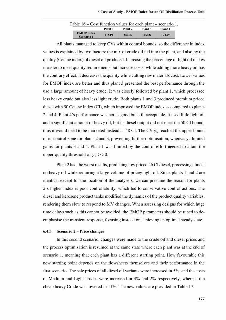
6 Case of Study - EMOP Index for an Oil Distillation Process Unit
177
Table 16 – Cost function values for each plant – scenario 1. Plant 1 Plant 2 Plant 3 Plant 4
EMOP Index Scenario 1
11819 24465 10758 12139
All plants managed to keep CVs within control bounds, so the difference in index
values is explained by two factors: the mix of crude oil fed into the plant, and also by the
quality (Cetane index) of diesel oil produced. Increasing the percentage of light oil makes
it easier to meet quality requirements but increase costs, while adding more heavy oil has
the contrary effect: it decreases the quality while cutting raw materials cost. Lower values
for EMOP index are better and thus plant 3 presented the best performance through the
use a large amount of heavy crude. It was closely followed by plant 1, which processed
less heavy crude but also less light crude. Both plants 1 and 3 produced premium priced
diesel with 50 Cetane Index (CI), which improved the EMOP index as compared to plants
2 and 4. Plant 4’s performance was not as good but still acceptable. It used little light oil
and a significant amount of heavy oil, but its diesel output did not meet the 50 CI bound,
thus it would need to be marketed instead as 48 CI. The CV y� reached the upper bound
of its control zone for plants 2 and 3, preventing further optimisation, whereas y® limited
gains for plants 3 and 4. Plant 1 was limited by the control effort needed to attain the
upper-quality threshold of w� > 50.
Plant 2 had the worst results, producing low priced 46 CI diesel, processing almost
no heavy oil while requiring a large volume of pricey light oil. Since plants 1 and 2 are
identical except for the location of the analysers, we can presume the reason for plants
2’s higher index is poor controllability, which led to conservative control actions. The
diesel and kerosene product tanks modified the dynamics of the product quality variables,
rendering them slow to respond to MV changes. When assessing designs for which huge
time delays such as this cannot be avoided, the EMOP parameters should be tuned to de-
emphasise the transient response, focusing instead on achieving an optimal steady state.
6.4.3 Scenario 2 – Price changes
In this second scenario, changes were made to the crude oil and diesel prices and
the process optimisation is resumed at the same state where each plant was at the end of
scenario 1, meaning that each plant has a different starting point. How favourable this
new starting point depends on the flowsheets themselves and their performance in the
first scenario. The sale prices of all diesel oil variants were increased in 5%, and the costs
of Medium and Light crudes were increased in 4% and 2% respectively, whereas the
cheap heavy Crude was lowered in 11%. The new values are provided in Table 17:
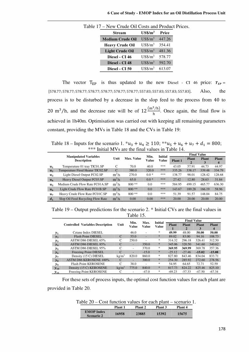
6 Case of Study - EMOP Index for an Oil Distillation Process Unit
178
Table 17 – New Crude Oil Costs and Product Prices.
Stream US$/m3 Price
Medium Crude Oil US$/m3 447.26
Heavy Crude Oil US$/m3 354.41
Light Crude Oil US$/m3 481.36
Diesel - CI 46 US$/m3 578.77
Diesel - CI 48 US$/m3 592.70
Diesel - CI 50 US$/m3 613.07
The vector T £ is thus updated to the new Diesel - CI 46 price: bcR =
µ578.77;578.77;578.77;578.77;578.77;578.77;578.77;557.83;557.83;557.83;557.83·. Also, the
process is to be disturbed by a decrease in the slop feed to the process from 40 to
20mW h⁄ , and the decrease rate will be of 12 Ô�s D⁄ ÖD . Once again, the final flow is
achieved in 1h40m. Optimisation was carried out with keeping all remaining parameters
constant, providing the MVs in Table 18 and the CVs in Table 19:
Table 18 – Inputs for the scenario 1. *fW + fv ≥ 110; **f� + f® + f¯ + ë� = 800; *** Initial MVs are the final values in Table 14.
Manipulated Variables Description
Unit Max. Value Min. Value
Initial Value
Final Value
Plant 1 Plant
2 Plant
3 Plant
4 �� Temperature 01 tray TIC01.SP C 70.0 40.0 *** 43.05 57.91 44.73 44.97 � Temperature Fired Heater TIC02.SP C 380.0 320.0 *** 335.26 338.17 339.48 334.79
�' Light Diesel Output FC02.SP m3/h 270.0 0.0 * *** 138.77 98.01 128.42 128.68
�© Heavy Diesel Output FC03.SP m3/h 65.0 0.0 * *** 27.42 12.80 28.63 31.84
�ª Medium Crude Flow Rate FC01A.SP m3/h 800 ** 0.0 *** 584.95 499.15 465.77 636.30
�« Light Crude Flow Rate FC01B.SP m3/h 800 ** 0.0 *** 143.67 189.28 166.19 58.96
�¬ Heavy Crude Flow Rate FC01C.SP m3/h 800 ** 0.0 *** 51.39 91.57 148.04 84.75
�� Slop Oil Feed Recycling Flow Rate m3/h 0.00 0.00 *** 20.00 20.00 20.00 20.00
Table 19 – Output predictions for the scenario 2. * Initial CVs are the final values in Table 15.
Controlled Variables Description Unit Min. Value
Max. Value
Initial Value
Final Value
Plant 1
Plant 2
Plant 3
Plant 4
�� Cetane Index DIESEL 46.0 - * 49.99 48.00 50.00 50.00
� Flash Point DIESEL C 55.0 - * 89.02 83.00 94.16 108.73
�' ASTM D86 DIESEL 65% C 250.0 - * 314.32 296.18 326.41 312.50
�© ASTM D86 DIESEL 85% C - 350.0 * 345.06 320.50 341.60 340.62
�ª ASTM D86 DIESEL 95% C - 370.0 * 369.95 369.99 369.78 357.36
�« Freezing Point DIESEL C - -15.0 * -25.12 -27.46 -15.02 -15.08 �¬ Density (15 C) DIESEL kg/m3 820.0 860.0 * 827.80 843.46 834.04 833.71
� ASTM D86 KEROSENE 100% C - 300.0 * 254.30 285.92 272.60 278.56
�\ Flash Point KEROSENE C 38.0 - * 54.95 64.65 72.71 52.59
��¾ Density (15 C) KEROSENE kg/m3 775.0 840.0 * 817.73 824.22 825.46 825.10
��� Freezing Point KEROSENE C - -47.0 * -69.23 -57.33 -47.50 -67.34
For these sets of process inputs, the optimal cost function values for each plant are
provided in Table 20.
Table 20 – Cost function values for each plant – scenario 1. Plant 1 Plant 2 Plant 3 Plant 4
EMOP Index Scenario 2
16958 23885 15392 15675
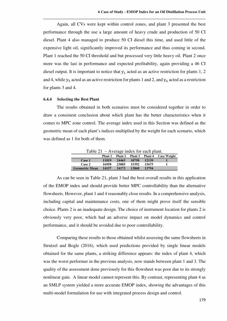
6 Case of Study - EMOP Index for an Oil Distillation Process Unit
179
Again, all CVs were kept within control zones, and plant 3 presented the best
performance through the use a large amount of heavy crude and production of 50 CI
diesel. Plant 4 also managed to produce 50 CI diesel this time, and used little of the
expensive light oil, significantly improved its performance and thus coming in second.
Plant 1 reached the 50 CI threshold and but processed very little heavy oil. Plant 2 once
more was the last in performance and expected profitability, again providing a 46 CI
diesel output. It is important to notice that y� acted as an active restriction for plants 1, 2
and 4, while y� acted as an active restriction for plants 1 and 2, and y® acted as a restriction
for plants 3 and 4.
6.4.4 Selecting the Best Plant
The results obtained in both scenarios must be considered together in order to
draw a consistent conclusion about which plant has the better characteristics when it
comes to MPC zone control. The average index used in this Section was defined as the
geometric mean of each plant’s indices multiplied by the weight for each scenario, which
was defined as 1 for both of them.
Table 21 – Average index for each plant. Plant 1 Plant 2 Plant 3 Plant 4 Case Weight
Case 1 11819 24465 10758 12139 1 Case 2 16958 23885 15392 15675 1
Geometric Mean 14157 24173 12868 13794
As can be seen in Table 21, plant 3 had the best overall results in this application
of the EMOP index and should provide better MPC controllability than the alternative
flowsheets. However, plant 1 and 4 reasonably close results. In a comprehensive analysis,
including capital and maintenance costs, one of them might prove itself the sensible
choice. Plants 2 is an inadequate design. The choice of instrument location for plants 2 is
obviously very poor, which had an adverse impact on model dynamics and control
performance, and it should be avoided due to poor controllability.
Comparing these results to those obtained whilst assessing the same flowsheets in
Strutzel and Bogle (2016), which used predictions provided by single linear models
obtained for the same plants, a striking difference appears: the index of plant 4, which
was the worst performer in the previous analysis, now stands between plant 1 and 3. The
quality of the assessment done previously for this flowsheet was poor due to its strongly
nonlinear gain. A linear model cannot represent this. By contrast, representing plant 4 as
an SMLP system yielded a more accurate EMOP index, showing the advantages of this
multi-model formulation for use with integrated process design and control.
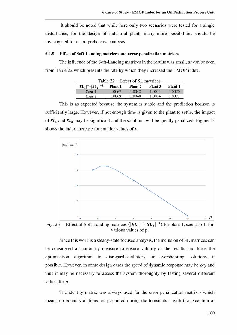
6 Case of Study - EMOP Index for an Oil Distillation Process Unit
180
It should be noted that while here only two scenarios were tested for a single
disturbance, for the design of industrial plants many more possibilities should be
investigated for a comprehensive analysis.
6.4.5 Effect of Soft-Landing matrices and error penalization matrices
The influence of the Soft-Landing matrices in the results was small, as can be seen
from Table 22 which presents the rate by which they increased the EMOP index.
Table 22 – Effect of SL matrices. |ÍÎ�|.�|ÍÎ |.� Plant 1 Plant 2 Plant 3 Plant 4
Case 1 1.0067 1.0048 1.0074 1.0070 Case 2 1.0069 1.0048 1.0074 1.0072
This is as expected because the system is stable and the prediction horizon is
sufficiently large. However, if not enough time is given to the plant to settle, the impact
of _`� and _` may be significant and the solutions will be greatly penalized. Figure 13
shows the index increase for smaller values of �:
Fig. 26 – Effect of Soft-Landing matrices k|_`�|.�|_` |.�m for plant 1, scenario 1, for
various values of �.
Since this work is a steady-state focused analysis, the inclusion of SL matrices can
be considered a cautionary measure to ensure validity of the results and force the
optimisation algorithm to disregard oscillatory or overshooting solutions if
possible. However, in some design cases the speed of dynamic response may be key and
thus it may be necessary to assess the system thoroughly by testing several different
values for �.
The identity matrix was always used for the error penalization matrix - which
means no bound violations are permitted during the transients – with the exception of
6 Case of Study - EMOP Index for an Oil Distillation Process Unit
181
plant 2 in scenario 2 where |cR| = 1.0104 to allow w� < w�'*,� over the whole predicted
range.
6.4.6 Optimisation algorithm and computational cost
The optimisation problem was solved using the interior-point routine available in
the optimisation toolbox in MATLAB. It is also worth noting that the problem has
nonlinear constraints and required a solver able to deal with disjunctive programming.
The results proved to be sensitive to the initial point chosen, and the optimisation
algorithm often reached a local minimum instead of a global one. To avoid this
shortcoming an iterative “genetic” algorithm strategy was implemented consisting of
using the previous solution the new starting point, but randomly modifying it so as to
implement “mutations”, then evaluating the cost function and storing the new solution if
it was better than the at least one of the 15 best previous ones. In this case, the worst
solution among the set of 15 was dropped and replaced by the new, better solution. The
random mutations were constrained to be within ±15% of the acceptable range for each
manipulated variable, and 15000 iterations were performed for each plant and case
studied. The fact that, in both scenarios, one or more CVs correlated to product quality
were saturated at the end of the prediction horizon seems to suggest that the solutions
presented are global. Saturated CVs mean no slack left for further optimisation since the
use of a cheaper mix of raw materials or less energy would result in off-spec products
with zero market value. While we hold the belief that global solutions have been obtained,
no formal proof can be provided due to the nonlinear nature of the optimisation problem
(introduced by varying weights and restrictions).
The same method was used as well for regression analysis problem given by Eq.
97 and Eq. 109, so the best fit could be obtained for the parameters of the degradation
functions. At the time of writing, even if linear models are used, solving the economic
MPC optimisation index involves a significant computational cost when dealing with
complex systems. For example, the problem described in Section 6 was solved using
MATLAB® R2016b running on a 3GHz quad-core Intel Xeon E5-1607 CPU, of which
50% of its capacity was available to the solver. In this condition, each iteration of the
method took between 5 and 15 seconds, so a typical simulation would take 40h or so.
However, the computational demand can be lowered by using smaller control or
prediction horizons, � and �. Using � = 1 reduced the computing time used by each
iteration to only 2-4 seconds. Setting � as high as possible is recommended, since it
enables additional degrees of freedom for the algorithm, which in turn leads to less
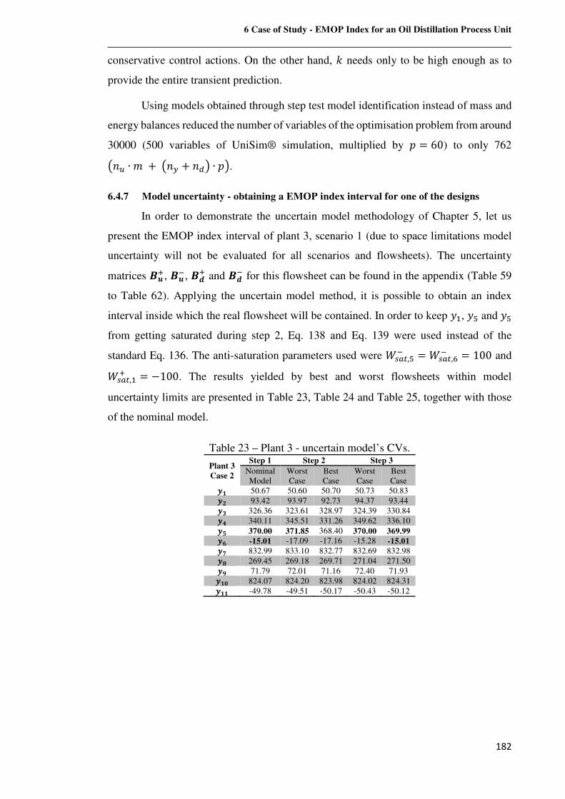
6 Case of Study - EMOP Index for an Oil Distillation Process Unit
182
conservative control actions. On the other hand, � needs only to be high enough as to
provide the entire transient prediction.
Using models obtained through step test model identification instead of mass and
energy balances reduced the number of variables of the optimisation problem from around
30000 (500 variables of UniSim® simulation, multiplied by � = 60) to only 762
ÔMP ∙ � +ÔMQ + M,Ö ∙ �Ö.
6.4.7 Model uncertainty - obtaining a EMOP index interval for one of the designs
In order to demonstrate the uncertain model methodology of Chapter 5, let us
present the EMOP index interval of plant 3, scenario 1 (due to space limitations model
uncertainty will not be evaluated for all scenarios and flowsheets). The uncertainty
matrices ��|, ��., ��| and ��. for this flowsheet can be found in the appendix (Table 59
to Table 62). Applying the uncertain model method, it is possible to obtain an index
interval inside which the real flowsheet will be contained. In order to keep w�, w� and w�
from getting saturated during step 2, Eq. 138 and Eq. 139 were used instead of the
standard Eq. 136. The anti-saturation parameters used were ��?@,�. =��?@,®. = 100 and ��?@,�| = −100. The results yielded by best and worst flowsheets within model
uncertainty limits are presented in Table 23, Table 24 and Table 25, together with those
of the nominal model.
Table 23 – Plant 3 - uncertain model’s CVs.
Plant 3 Case 2
Step 1 Step 2 Step 3
Nominal Model
Worst Case
Best Case
Worst Case
Best Case
�� 50.67 50.60 50.70 50.73 50.83
� 93.42 93.97 92.73 94.37 93.44
�' 326.36 323.61 328.97 324.39 330.84
�© 340.11 345.51 331.26 349.62 336.10
�ª 370.00 371.85 368.40 370.00 369.99
�« -15.01 -17.09 -17.16 -15.28 -15.01
�¬ 832.99 833.10 832.77 832.69 832.98
� 269.45 269.18 269.71 271.04 271.50
�\ 71.79 72.01 71.16 72.40 71.93
��¾ 824.07 824.20 823.98 824.02 824.31
��� -49.78 -49.51 -50.17 -50.43 -50.12
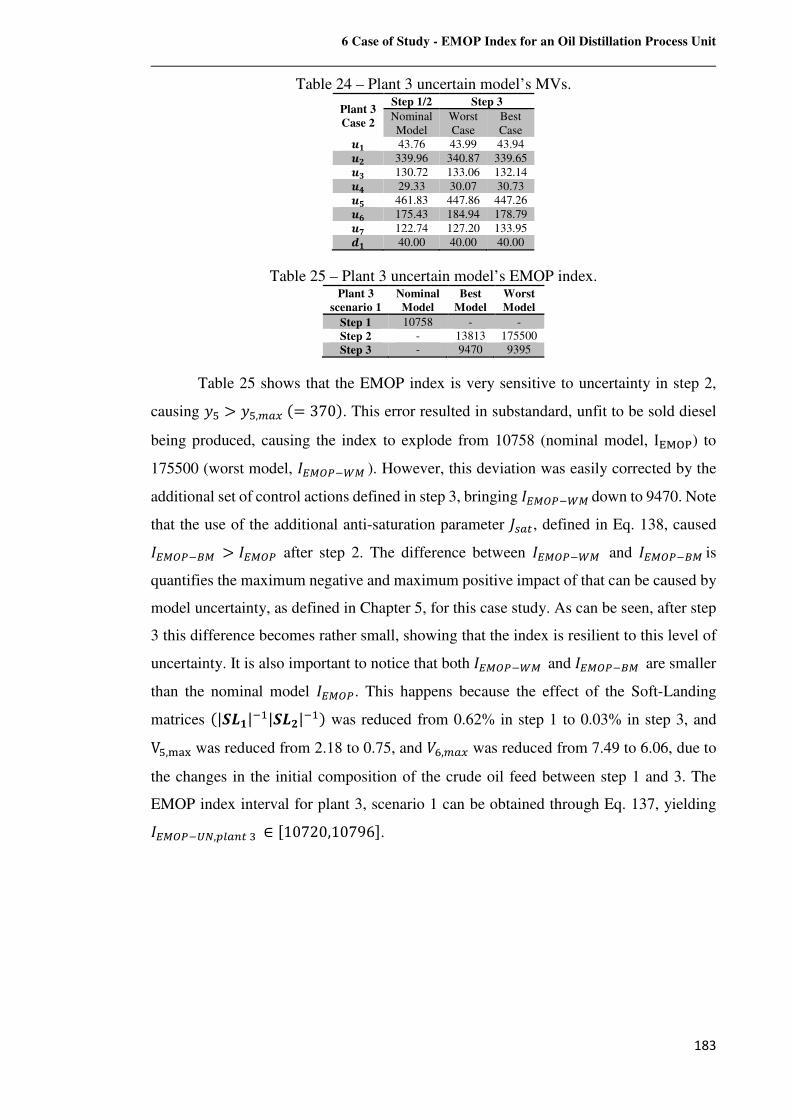
6 Case of Study - EMOP Index for an Oil Distillation Process Unit
183
Table 24 – Plant 3 uncertain model’s MVs.
Plant 3 Case 2
Step 1/2 Step 3
Nominal Model
Worst Case
Best Case
�� 43.76 43.99 43.94
� 339.96 340.87 339.65
�' 130.72 133.06 132.14
�© 29.33 30.07 30.73
�ª 461.83 447.86 447.26
�« 175.43 184.94 178.79
�¬ 122.74 127.20 133.95
�� 40.00 40.00 40.00
Table 25 – Plant 3 uncertain model’s EMOP index. Plant 3
scenario 1 Nominal Model
Best Model
Worst Model
Step 1 10758 - - Step 2 - 13813 175500 Step 3 - 9470 9395
Table 25 shows that the EMOP index is very sensitive to uncertainty in step 2,
causing w� > w�,�?�k= 370m. This error resulted in substandard, unfit to be sold diesel
being produced, causing the index to explode from 10758 (nominal model, I ¡¢£) to
175500 (worst model, 23456.:4). However, this deviation was easily corrected by the
additional set of control actions defined in step 3, bringing 23456.:4down to 9470. Note
that the use of the additional anti-saturation parameter ;�?@, defined in Eq. 138, caused
23456.74 > 23456 after step 2. The difference between 23456.:4 and 23456.74is
quantifies the maximum negative and maximum positive impact of that can be caused by
model uncertainty, as defined in Chapter 5, for this case study. As can be seen, after step
3 this difference becomes rather small, showing that the index is resilient to this level of
uncertainty. It is also important to notice that both 23456.:4 and 23456.74 are smaller
than the nominal model 23456. This happens because the effect of the Soft-Landing
matrices k|_`�|.�|_` |.�m was reduced from 0.62% in step 1 to 0.03% in step 3, and
V�,��¾ was reduced from 2.18 to 0.75, and -®,�?� was reduced from 7.49 to 6.06, due to
the changes in the initial composition of the crude oil feed between step 1 and 3. The
EMOP index interval for plant 3, scenario 1 can be obtained through Eq. 137, yielding
23456.89,N)?*@W ∈ µ10720,10796·.
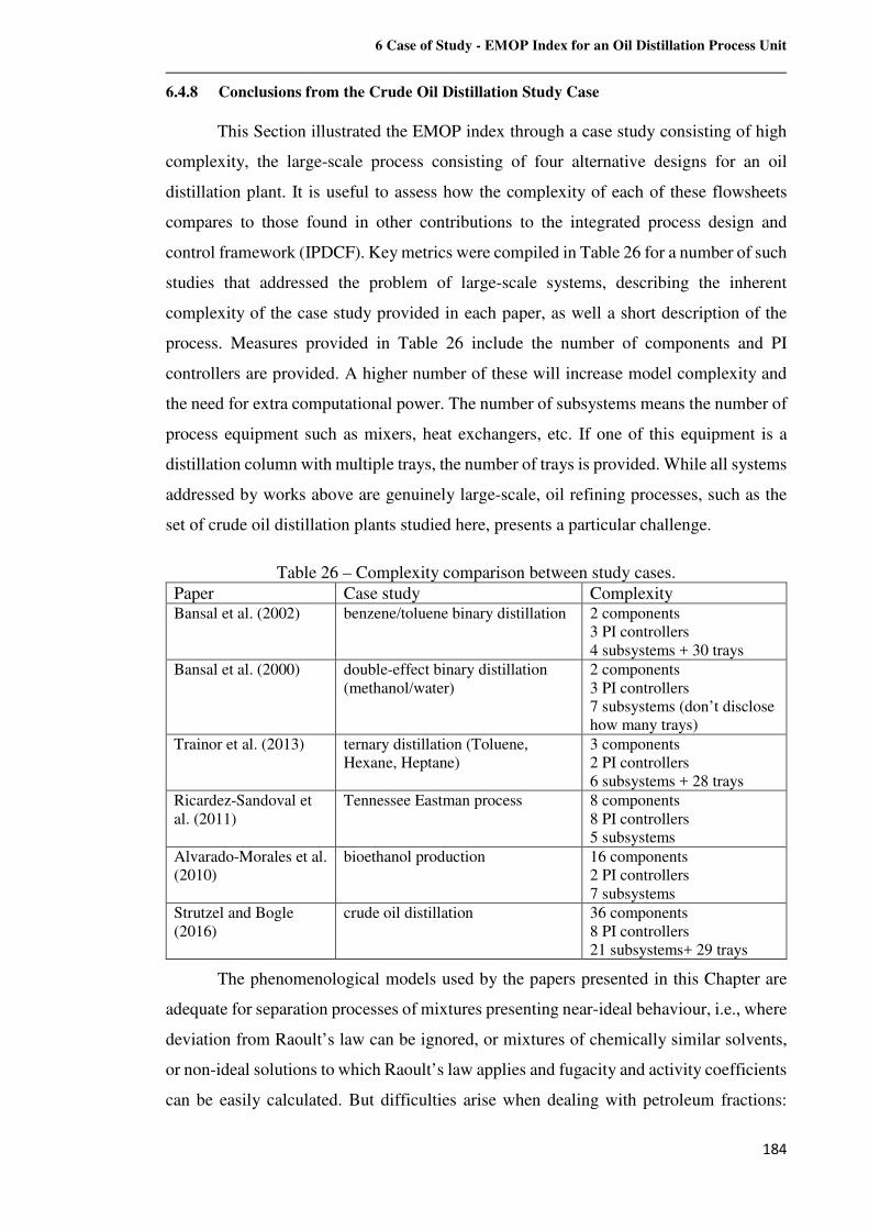
6 Case of Study - EMOP Index for an Oil Distillation Process Unit
184
6.4.8 Conclusions from the Crude Oil Distillation Study Case
This Section illustrated the EMOP index through a case study consisting of high
complexity, the large-scale process consisting of four alternative designs for an oil
distillation plant. It is useful to assess how the complexity of each of these flowsheets
compares to those found in other contributions to the integrated process design and
control framework (IPDCF). Key metrics were compiled in Table 26 for a number of such
studies that addressed the problem of large-scale systems, describing the inherent
complexity of the case study provided in each paper, as well a short description of the
process. Measures provided in Table 26 include the number of components and PI
controllers are provided. A higher number of these will increase model complexity and
the need for extra computational power. The number of subsystems means the number of
process equipment such as mixers, heat exchangers, etc. If one of this equipment is a
distillation column with multiple trays, the number of trays is provided. While all systems
addressed by works above are genuinely large-scale, oil refining processes, such as the
set of crude oil distillation plants studied here, presents a particular challenge.
Table 26 – Complexity comparison between study cases.
Paper Case study Complexity Bansal et al. (2002) benzene/toluene binary distillation 2 components
3 PI controllers 4 subsystems + 30 trays
Bansal et al. (2000) double-effect binary distillation (methanol/water)
2 components 3 PI controllers 7 subsystems (don’t disclose how many trays)
Trainor et al. (2013) ternary distillation (Toluene, Hexane, Heptane)
3 components 2 PI controllers 6 subsystems + 28 trays
Ricardez-Sandoval et al. (2011)
Tennessee Eastman process 8 components 8 PI controllers 5 subsystems
Alvarado-Morales et al. (2010)
bioethanol production 16 components 2 PI controllers 7 subsystems
Strutzel and Bogle (2016)
crude oil distillation 36 components 8 PI controllers 21 subsystems+ 29 trays
The phenomenological models used by the papers presented in this Chapter are
adequate for separation processes of mixtures presenting near-ideal behaviour, i.e., where
deviation from Raoult’s law can be ignored, or mixtures of chemically similar solvents,
or non-ideal solutions to which Raoult’s law applies and fugacity and activity coefficients
can be easily calculated. But difficulties arise when dealing with petroleum fractions:

6 Case of Study - EMOP Index for an Oil Distillation Process Unit
185
each subsystem usually has dozens of non-ideal hypothetical components; severe
operating conditions mean that the behaviour of gases, solutions and mixtures is also non-
ideal; multiphase flow is very common and hard to model adequately; equipment designs
are intricate. The best simulators for this kind of process do not provide their set of
equations, which are closed-source intellectual property. For all these reasons, and the
time and engineering effort required for rigorous modelling is always very large and,
unless models are linearised, even with the optimisation solvers and processing power
available at the time of writing it is doubtful that a solution could be found in reasonable
time. This Thesis aims to offer an alternative Controllability Analysis approach that is
better suited for the plant-wide design of oil refining processes, and also to include the
use of Model Predictive Control as the main control strategy. With this goal in mind, the
use of commercial simulation packages for modelling was very successful as none of the
IPDCF case studies in the benchmark matches the complexity and scale of the problem
presented in this Section.
7 Comparison between two Integrated Process Design and Control Methodologies
186
7 Comparison between two Integrated Process
Design and Control Methodologies
In this Section, the Economic MPC Optimisation index is applied to the case study
provided in Francisco et al. (2011), with the goal of enabling comparison between it and
another methodology available in open literature. Both works s can be classified as
Integrated Process Design and Control methods specially designed for flowsheets
controlled by MPC schemes.
However, they possess different characteristics and goals. As detailed in Section
2.3.1, Francisco et al. (2011) present a synthesis method for the obtaining of new
flowsheet designs by evaluating MPC performance. It combines controllability and
economic indexes that are evaluated at each iteration as key plant parameters are changed.
The EMOP index is used to assess the optimal operating point of a given flowsheet and
finding the optimal trajectory to reach it, which is restricted by the control zones of the
MPC scheme. The purpose of this comparison is determining whether the differences
between methods can lead to different plant assessment.
To ensure the equivalence of models while comparing the methods, a
phenomenological nonlinear state-space model will be used to represent several designs
for the activated sludge process (ASP) of a wastewater treatment plant. Unlike the case
study of the atmospheric distillation plant of Chapter 6, the numerical complexity is low
for obtaining the dynamic response of the ASP. Thus, another goal is assessing the
computational demands posed by the use of a small-scale nonlinear model, as compared
to the large-scale linear model described in Chapter 6.
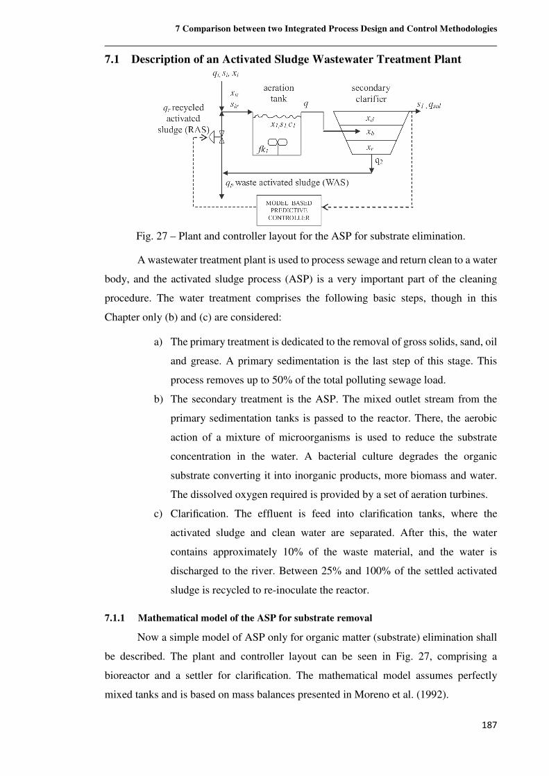
7 Comparison between two Integrated Process Design and Control Methodologies
187
7.1 Description of an Activated Sludge Wastewater Treatment Plant
Fig. 27 – Plant and controller layout for the ASP for substrate elimination.
A wastewater treatment plant is used to process sewage and return clean to a water
body, and the activated sludge process (ASP) is a very important part of the cleaning
procedure. The water treatment comprises the following basic steps, though in this
Chapter only (b) and (c) are considered:
a) The primary treatment is dedicated to the removal of gross solids, sand, oil
and grease. A primary sedimentation is the last step of this stage. This
process removes up to 50% of the total polluting sewage load.
b) The secondary treatment is the ASP. The mixed outlet stream from the
primary sedimentation tanks is passed to the reactor. There, the aerobic
action of a mixture of microorganisms is used to reduce the substrate
concentration in the water. A bacterial culture degrades the organic
substrate converting it into inorganic products, more biomass and water.
The dissolved oxygen required is provided by a set of aeration turbines.
c) Clarification. The effluent is feed into clarification tanks, where the
activated sludge and clean water are separated. After this, the water
contains approximately 10% of the waste material, and the water is
discharged to the river. Between 25% and 100% of the settled activated
sludge is recycled to re-inoculate the reactor.
7.1.1 Mathematical model of the ASP for substrate removal
Now a simple model of ASP only for organic matter (substrate) elimination shall
be described. The plant and controller layout can be seen in Fig. 27, comprising a
bioreactor and a settler for clarification. The mathematical model assumes perfectly
mixed tanks and is based on mass balances presented in Moreno et al. (1992).
7 Comparison between two Integrated Process Design and Control Methodologies
188
7.1.1.1 Mass balance for the aeration tanks
The rate of change of the biomass, organic substrate and dissolved oxygen
concentrations are given by:
,��,@ = ��?�wC ����
k=¦|��m−A, ��p�� − A,u� + >
=� ku'H − u�m Eq. 168
,��,@ = −��?� ����
k=¦|��m− +(,A, ��p�� + +(,ACu� + >
=� k^'H − ^�m Eq. 169
,C�,@ = A)?+(�k�� − ��m − ��� −
>=� �� Eq. 170
where u�, ^� and �� are the biomass, substrate (Chemical Oxygen Demand, COD)
and dissolved oxygen (DO) concentration at the output of the aeration tanks (mg/l); u'H and ^'H are respectively the inlet biomass and substrate (mg/l). ��?� is the maximum
growth rate of the microorganisms, � is the inlet flow (m3/h), A, is the kinetic coefficient
of biomass decay by endogenous metabolism (1/h), AC is the kinetic coefficient of
biomass decay by biological waste, -� is the total useful volume for the six aeration tanks
(m3), wC is the yield coefficient between cellular growth and substrate elimination, +(, is
the yield coefficient between biomass endogenous and substrate contribution to the
medium, �� is the DO concentration at saturation, A)? is the mass transfer coefficient, +(�
is the aeration factor which depends on the number and speed of working turbines, OUR
is the oxygen uptake rate and A� is the saturation constant.
For the biomass rate of change, the first term describes the biomass growth
according to the Monod model, the second describes cell death, the third describes the
biological waste, and the final term quantifies the dilution effects. For the rate of
consumption of organic substrate, the first term expresses the decrease of the substrate
through the activity of the biomass (Monod model), the second and third ones describe
the transformation part of the dead biomass and biological waste into organic substrate,
and the last term is the difference between the input and output substrate mass flow.
For the dissolved oxygen concentration, the Eq. 169 follows the classic literature:
the first term is the rate of oxygen transferred to the water, the second describes the rate
of oxygen used by the microorganisms (uptake rate), and the final term quantifies the
dilution effects. Algebraic equations for u'Hand ^'H are expressed as mass balances:
7 Comparison between two Integrated Process Design and Control Methodologies
189
u'H = �x>x|�S>S> Eq. 171
^'H = �x>x|��>S> Eq. 172
where u', ^' are the biomass and substrate at the influent, �' is the input flow to
the process. uH and �H are the recycle concentrations and flow rate. The equation for
oxygen uptake rate is:
��� = −AB���?� ����k=¦|��m Eq. 173
where AB� is the yield coefficient between the cellular growth and the oxygen
consumption rate.
7.1.1.2 Mass balance for the secondary clarifiers (settlers)
The operation of these elements is described by mass balance equations and one
expression for the settling of activated sludge. The model considers the difference in
settling rates between layers of increasing biomass concentration.
This model attempts to capture the dynamic behaviour of the clarifiers:
��F, ,��,@ = ��?)uG − ��?)u, − ��U�ku,m Eq. 174
��FG ,�Ï,@ = �u� − ��?)uG − ��uG + ��U�ku,m − ��U�kuGm Eq. 175
��FH ,�S,@ = ��uG − ��uH − ��U�kuGm Eq. 176
whereu, is the biomass concentration at the surface of the settler leaving the
plant, ��?) is the flow of clean water at the output of the settler, uG is the biomass
concentration in the second layer, �� is the activated sludge total recycling flow, uH is the
biomass concentration at the bottom of the settler, U� is the settling rate of the activated
sludge, �� is the area of the settler, and F,, FG , FH are the height of the first, second and
third layer, respectively (Fig. 27). Note that the settler input flow � enters to the unit at
the second layer level. The settling rate parameters are fitted to a curve provided by pilot
plants:
7 Comparison between two Integrated Process Design and Control Methodologies
190
U�kuGm = M�uG"k.?H�Ïm Eq. 177
U�ku,m = M�u,"k.?H��m Eq. 178
The relations between the different flow rates are:
� = �' + �H Eq. 179
��?) = �' − �N Eq. 180
�� = �H + �N Eq. 181
where �N is the purge flow. The control of this process aims to keep the substrate
at the output (^�) below the legal requirement value despite the large variations of the
flow rate (�') and the substrate concentration of the incoming water (^'). The disturbances
vector is: d = k^', �'m. The recycling flow (�H) is the manipulated variable, and the
controlled output is the substrate (^�) in the reactor: fk�m = �H; wk�m = ^�. Biomass (u�)
in the reactor is a bounded variable. Table 27 provides a symbol list for the variables and
parameters of the activated sludge process, as well as their units and values when
convenient.
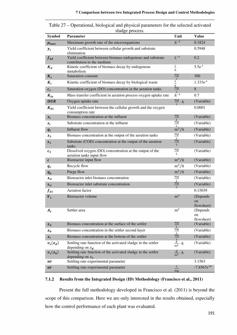
7 Comparison between two Integrated Process Design and Control Methodologies
191
Table 27 – Operational, biological and physical parameters for the selected activated sludge process.
Symbol Parameter Unit Value
¤�� Maximum growth rate of the microorganisms ℎ.� 0.1824
�° Yield coefficient between cellular growth and substrate elimination
0.5948
Ü\� Yield coefficient between biomass endogenous and substrate contribution to the medium
�.� 0.2
!� Kinetic coefficient of biomass decay by endogenous metabolism
é³ 5.5e-5
!i Saturation constant �?é 300
!° Kinetic coefficient of biomass decay by biological waste é³ 1.333e-4
°i Saturation oxygen (DO) concentration in the aeration tanks �?é 8
!�� Mass transfer coefficient in aeration process oxygen uptake rate ℎ.� 0.7
±gZ Oxygen uptake rate �?é ∙ ℎ (Variable)
!¾� Yield coefficient between the cellular growth and the oxygen consumption rate
0.0001
V Biomass concentration at the influent �?é (Variable)
iV Substrate concentration at the influent �?é (Variable)
�V Influent flow �W ℎ⁄ (Variable)
� Biomass concentration at the output of the aeration tanks �?é (Variable)
i� Substrate (COD) concentration at the output of the aeration tanks
�?é (Variable)
°� Dissolved oxygen (DO) concentration at the output of the aeration tanks input flow
�?é (Variable)
° Bioreactor input flow �W ℎ⁄ (Variable)
�T Recycle flow �W ℎ⁄ (Variable)
�Y Purge flow �W ℎ⁄ (Variable)
VT Bioreactor inlet biomass concentration �?é (Variable)
iVT Bioreactor inlet substrate concentration �?é (Variable)
Ü\� Aeration factor
0.15039
j� Bioreactor volume �W (Depends on flowsheet)
�i Settler area �� (Depends on flowsheet)
� Biomass concentration at the surface of the settler �?é (Variable)
l Biomass concentration in the settler second layer �?é (Variable)
T Biomass concentration at the bottom of the settler �?é (Variable)
�ik�m Settling rate function of the activated sludge in the settler depending on u�
?�p ∙ ℎ (Variable)
�iklm Settling rate function of the activated sludge in the settler depending on uG
?�p ∙ ℎ (Variable)
hT Settling rate experimental parameter
3.1563
�T Settling rate experimental parameter � -7.8567e-04
7.1.2 Results from the Integrated Design (ID) Methodology (Francisco et al., 2011)
Present the full methodology developed in Francisco et al. (2011) is beyond the
scope of this comparison. Here we are only interested in the results obtained, especially
how the control performance of each plant was evaluated.
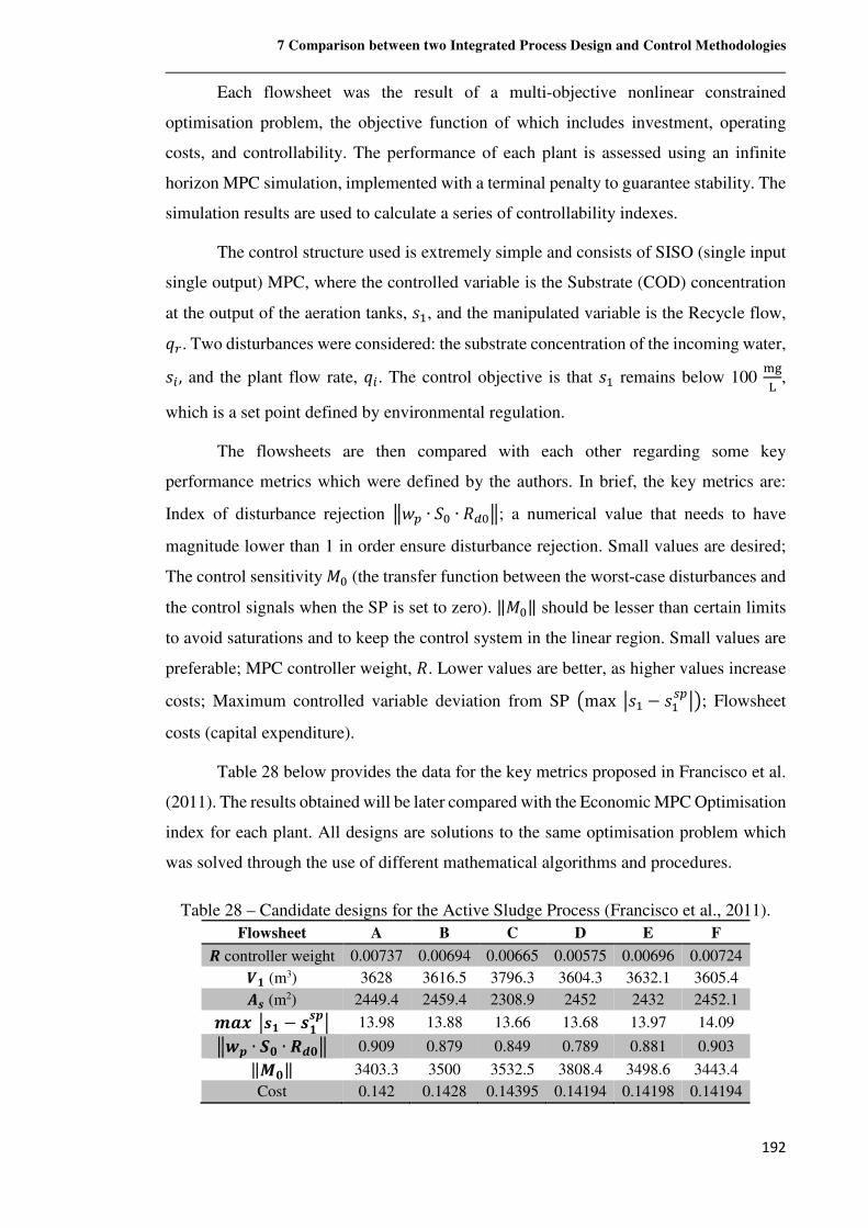
7 Comparison between two Integrated Process Design and Control Methodologies
192
Each flowsheet was the result of a multi-objective nonlinear constrained
optimisation problem, the objective function of which includes investment, operating
costs, and controllability. The performance of each plant is assessed using an infinite
horizon MPC simulation, implemented with a terminal penalty to guarantee stability. The
simulation results are used to calculate a series of controllability indexes.
The control structure used is extremely simple and consists of SISO (single input
single output) MPC, where the controlled variable is the Substrate (COD) concentration
at the output of the aeration tanks, ^�, and the manipulated variable is the Recycle flow,
�H. Two disturbances were considered: the substrate concentration of the incoming water,
^', and the plant flow rate, �'. The control objective is that ^� remains below 100 ��� ,
which is a set point defined by environmental regulation.
The flowsheets are then compared with each other regarding some key
performance metrics which were defined by the authors. In brief, the key metrics are:
Index of disturbance rejection kÐN ∙ �B ∙ �,Bk; a numerical value that needs to have
magnitude lower than 1 in order ensure disturbance rejection. Small values are desired;
The control sensitivity IB (the transfer function between the worst-case disturbances and
the control signals when the SP is set to zero). ‖IB‖ should be lesser than certain limits
to avoid saturations and to keep the control system in the linear region. Small values are
preferable; MPC controller weight, �. Lower values are better, as higher values increase
costs; Maximum controlled variable deviation from SP Ômax Ø^� − �̂�NØÖ; Flowsheet
costs (capital expenditure).
Table 28 below provides the data for the key metrics proposed in Francisco et al.
(2011). The results obtained will be later compared with the Economic MPC Optimisation
index for each plant. All designs are solutions to the same optimisation problem which
was solved through the use of different mathematical algorithms and procedures.
Table 28 – Candidate designs for the Active Sludge Process (Francisco et al., 2011).
Flowsheet A B C D E F
Z controller weight 0.00737 0.00694 0.00665 0.00575 0.00696 0.00724
j� (m3) 3628 3616.5 3796.3 3604.3 3632.1 3605.4
�i (m2) 2449.4 2459.4 2308.9 2452 2432 2452.1
�� Øi� − i�iYØ 13.98 13.88 13.66 13.68 13.97 14.09 keY ∙ _¾ ∙ Z�¾k 0.909 0.879 0.849 0.789 0.881 0.903
‖¾‖ 3403.3 3500 3532.5 3808.4 3498.6 3443.4
Cost 0.142 0.1428 0.14395 0.14194 0.14198 0.14194
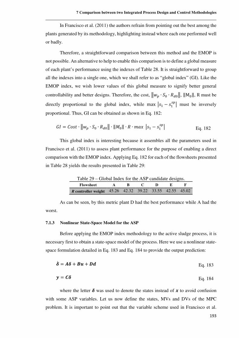
7 Comparison between two Integrated Process Design and Control Methodologies
193
In Francisco et al. (2011) the authors refrain from pointing out the best among the
plants generated by its methodology, highlighting instead where each one performed well
or badly.
Therefore, a straightforward comparison between this method and the EMOP is
not possible. An alternative to help to enable this comparison is to define a global measure
of each plant’s performance using the indexes of Table 28. It is straightforward to group
all the indexes into a single one, which we shall refer to as “global index” (GI). Like the
EMOP index, we wish lower values of this global measure to signify better general
controllability and better designs. Therefore, the cost, kÐN ∙ �B ∙ �,Bk, ‖MB‖, R must be
directly proportional to the global index, while max Ø^� − �̂�NØ must be inversely
proportional. Thus, GI can be obtained as shown in Eq. 182:
�2 = ÊÑ^¿ ∙ kÐN ∙ �B ∙ �,Bk ∙ ‖IB‖ ∙ � ∙ �~u Ø^� − �̂�NØ Eq. 182
This global index is interesting because it assembles all the parameters used in
Francisco et al. (2011) to assess plant performance for the purpose of enabling a direct
comparison with the EMOP index. Applying Eq. 182 for each of the flowsheets presented
in Table 28 yields the results presented in Table 29:
Table 29 – Global Index for the ASP candidate designs.
Flowsheet A B C D E F
R controller weight 45.26 42.32 39.22 33.55 42.55 45.02
As can be seen, by this metric plant D had the best performance while A had the
worst.
7.1.3 Nonlinear State-Space Model for the ASP
Before applying the EMOP index methodology to the active sludge process, it is
necessary first to obtain a state-space model of the process. Here we use a nonlinear state-
space formulation detailed in Eq. 183 and Eq. 184 to provide the output prediction:
�¼ = �� + �� + � Eq. 183
� = �� Eq. 184
where the letter � was used to denote the states instead of to avoid confusion
with some ASP variables. Let us now define the states, MVs and DVs of the MPC
problem. It is important to point out that the variable scheme used in Francisco et al.
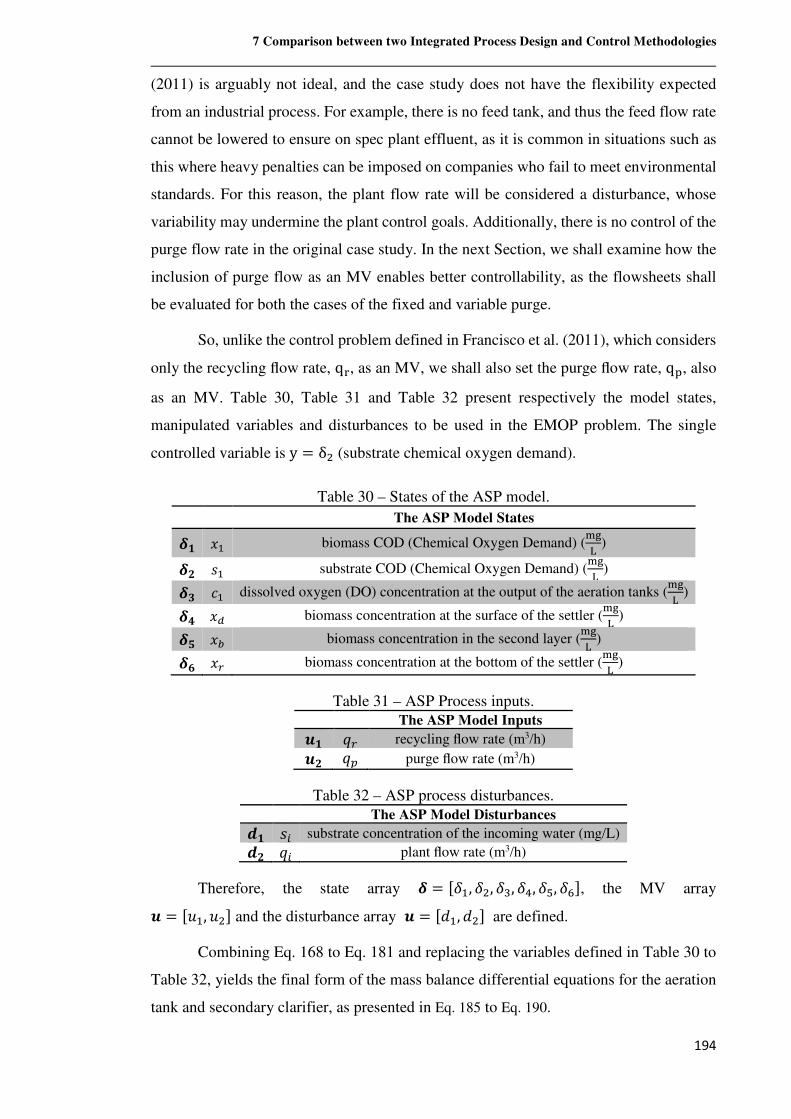
7 Comparison between two Integrated Process Design and Control Methodologies
194
(2011) is arguably not ideal, and the case study does not have the flexibility expected
from an industrial process. For example, there is no feed tank, and thus the feed flow rate
cannot be lowered to ensure on spec plant effluent, as it is common in situations such as
this where heavy penalties can be imposed on companies who fail to meet environmental
standards. For this reason, the plant flow rate will be considered a disturbance, whose
variability may undermine the plant control goals. Additionally, there is no control of the
purge flow rate in the original case study. In the next Section, we shall examine how the
inclusion of purge flow as an MV enables better controllability, as the flowsheets shall
be evaluated for both the cases of the fixed and variable purge.
So, unlike the control problem defined in Francisco et al. (2011), which considers
only the recycling flow rate, qÀ, as an MV, we shall also set the purge flow rate, q2, also
as an MV. Table 30, Table 31 and Table 32 present respectively the model states,
manipulated variables and disturbances to be used in the EMOP problem. The single
controlled variable is y = δ� (substrate chemical oxygen demand).
Table 30 – States of the ASP model.
The ASP Model States
�� u� biomass COD (Chemical Oxygen Demand) (��� )
� ^� substrate COD (Chemical Oxygen Demand) (��� )
�' �� dissolved oxygen (DO) concentration at the output of the aeration tanks (��� )
�© u, biomass concentration at the surface of the settler (��� )
�ª uG biomass concentration in the second layer (��� )
�« uH biomass concentration at the bottom of the settler (��� )
Table 31 – ASP Process inputs. The ASP Model Inputs
�� �H recycling flow rate (m3/h)
� �N purge flow rate (m3/h)
Table 32 – ASP process disturbances. The ASP Model Disturbances
�� ^' substrate concentration of the incoming water (mg/L)
� �' plant flow rate (m3/h)
Therefore, the state array � = µÓ�, Ó�, ÓW, Óv, Ó�, Ó®·, the MV array � = µf�, f�· and the disturbance array � = µë�, ë�· are defined.
Combining Eq. 168 to Eq. 181 and replacing the variables defined in Table 30 to
Table 32, yields the final form of the mass balance differential equations for the aeration
tank and secondary clarifier, as presented in Eq. 185 to Eq. 190.
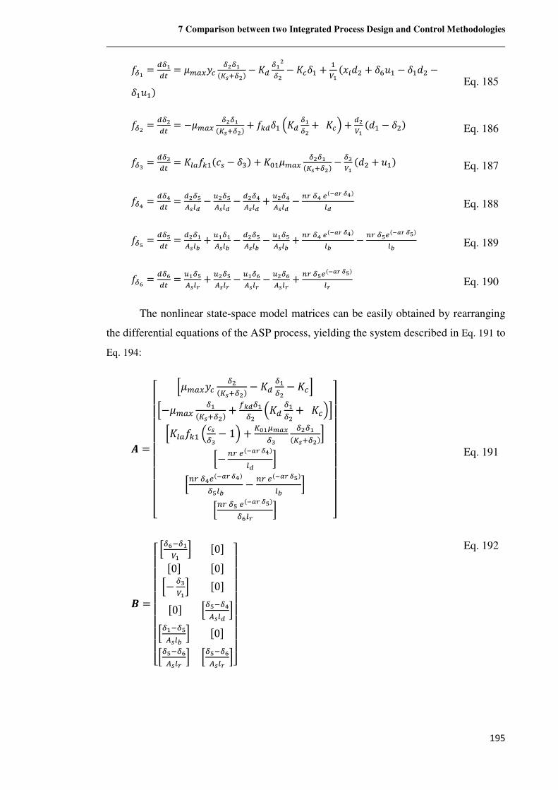
7 Comparison between two Integrated Process Design and Control Methodologies
195
+Ô� = ,Ô�,@ = ��?�wC ÔpÔ�
k=¦|Ôpm− A, Ô�pÔp − ACÓ� + �=� ku'ë� + Ó®f� − Ó�ë� −Ó�f�m Eq. 185
+Ôp = ,Ôp,@ = −��?� ÔpÔ�
k=¦|Ôpm+ +(,Ó� ÷A, Ô�Ôp +ACø + ,p=� kë� − Ó�m Eq. 186
+Ôs = ,Ôs,@ = A)?+(�k�� − ÓWm + AB���?� ÔpÔ�
k=¦|Ôpm− Ôs=� kë� + f�m Eq. 187
+Ôr = ,Ôr,@ =
,pÔ¹ñ¦)� − PpÔ¹
ñ¦)� − ,pÔrñ¦)� + PpÔr
ñ¦)� − *HÔrLk@QSÕrm)� Eq. 188
+Ô¹ = ,Ô¹,@ =
,pÔ�ñ¦)Ï + P�Ô�
ñ¦)Ï − ,pÔ¹ñ¦)Ï − P�Ô¹
ñ¦)Ï + *HÔrLk@QSÕrm)Ï − *HÔ¹Lk@QSÕ¹m
)Ï Eq. 189
+Ôº = ,Ôº,@ =
P�Ô¹ñ¦)S + PpÔ¹
ñ¦)S − P�Ôºñ¦)S − PpÔº
ñ¦)S + *HÔ¹Lk@QSÕ¹m)S Eq. 190
The nonlinear state-space model matrices can be easily obtained by rearranging
the differential equations of the ASP process, yielding the system described in Eq. 191 to
Eq. 194:
� =
����������� >��?�wC Ôp
k=¦|Ôpm− A, Ô�Ôp − ACC>−��?� Ô�k=¦|Ôpm+ )�Ô�Ôp ÷A, Ô�Ôp +ACøC>A)?+(� ÷C¦Ôs − 1ø + =t�Ö_Q�Ôs ÔpÔ�
k=¦|ÔpmC>− *HLk@QSÕrm)� C
>*HÔrLk@QSÕrmÔ¹)Ï − *HLk@QSÕ¹m)Ï C
>*HԹLk@QSչmԺ)S C ����������� Eq. 191
� =
���������� >Ժ.�
=� C µ0·µ0· µ0·>− Ôs
=�C µ0·
µ0· >Ô¹.Ôrñ¦)� C>Ô�.Ô¹
ñ¦)Ï C µ0·>Ô¹.Ôºñ¦)S C >Ô¹.Ôº
ñ¦)S C����������
Eq. 192
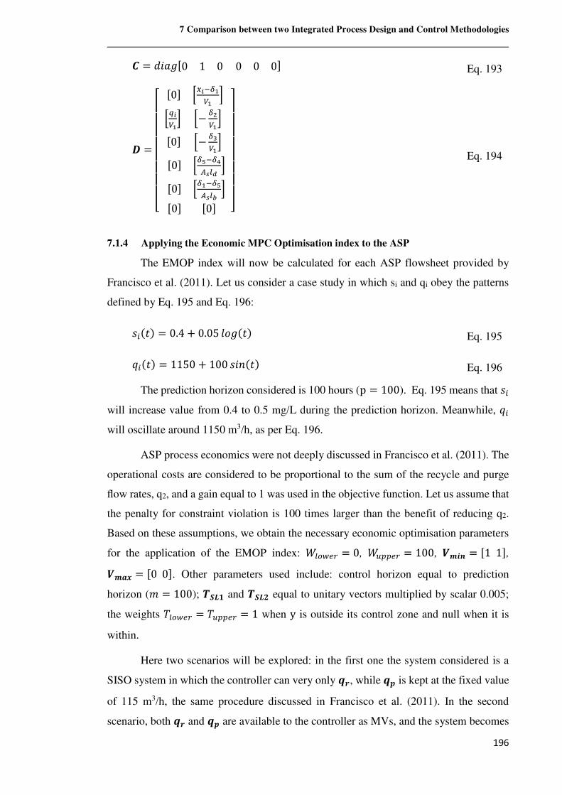
7 Comparison between two Integrated Process Design and Control Methodologies
196
� = ë¹~Aµ0 1 00 0 0· Eq. 193
=
����������µ0· >�x.Ô�
=� C>>x=�C >− Ôp
=�Cµ0· >− Ôs
=�Cµ0· >Ô¹.Ôr
ñ¦)� Cµ0· >Ô�.Ô¹
ñ¦)Ï Cµ0· µ0· ��
��������
Eq. 194
7.1.4 Applying the Economic MPC Optimisation index to the ASP
The EMOP index will now be calculated for each ASP flowsheet provided by
Francisco et al. (2011). Let us consider a case study in which si and qi obey the patterns
defined by Eq. 195 and Eq. 196:
^'k¿m = 0.4+ 0.05 FÑAk¿m Eq. 195
�'k¿m = 1150 + 100 ^¹Mk¿m Eq. 196
The prediction horizon considered is 100 hours (p = 100). Eq. 195 means that ^' will increase value from 0.4 to 0.5 mg/L during the prediction horizon. Meanwhile, �' will oscillate around 1150 m3/h, as per Eq. 196.
ASP process economics were not deeply discussed in Francisco et al. (2011). The
operational costs are considered to be proportional to the sum of the recycle and purge
flow rates, q2, and a gain equal to 1 was used in the objective function. Let us assume that
the penalty for constraint violation is 100 times larger than the benefit of reducing q2.
Based on these assumptions, we obtain the necessary economic optimisation parameters
for the application of the EMOP index: �)K�LH = 0, �PNNLH = 100, j�Vh = µ11·, j�� = µ00·. Other parameters used include: control horizon equal to prediction
horizon (� = 100); b_`� and b_` equal to unitary vectors multiplied by scalar 0.005;
the weights a)K�LH = aPNNLH = 1 when y is outside its control zone and null when it is
within.
Here two scenarios will be explored: in the first one the system considered is a
SISO system in which the controller can very only �T, while �Y is kept at the fixed value
of 115 m3/h, the same procedure discussed in Francisco et al. (2011). In the second
scenario, both �T and �Y are available to the controller as MVs, and the system becomes
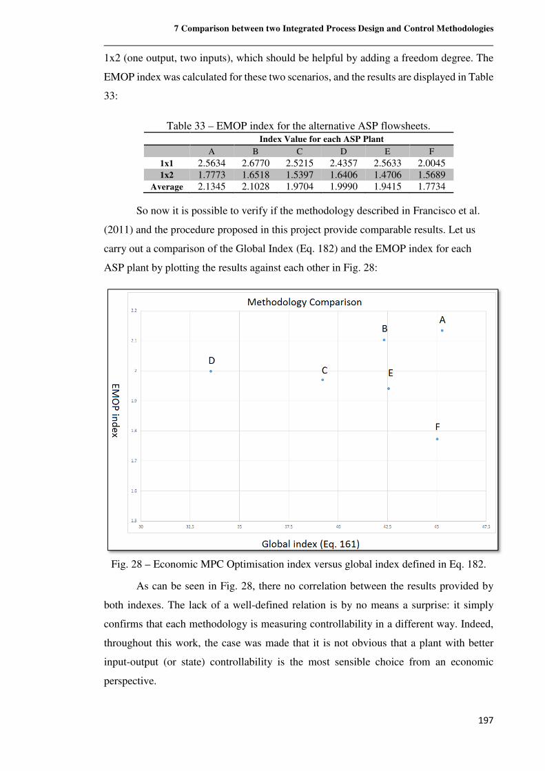
7 Comparison between two Integrated Process Design and Control Methodologies
197
1x2 (one output, two inputs), which should be helpful by adding a freedom degree. The
EMOP index was calculated for these two scenarios, and the results are displayed in Table
33:
Table 33 – EMOP index for the alternative ASP flowsheets. Index Value for each ASP Plant A B C D E F
1x1 2.5634 2.6770 2.5215 2.4357 2.5633 2.0045 1x2 1.7773 1.6518 1.5397 1.6406 1.4706 1.5689
Average 2.1345 2.1028 1.9704 1.9990 1.9415 1.7734
So now it is possible to verify if the methodology described in Francisco et al.
(2011) and the procedure proposed in this project provide comparable results. Let us
carry out a comparison of the Global Index (Eq. 182) and the EMOP index for each
ASP plant by plotting the results against each other in Fig. 28:
Fig. 28 – Economic MPC Optimisation index versus global index defined in Eq. 182.
As can be seen in Fig. 28, there no correlation between the results provided by
both indexes. The lack of a well-defined relation is by no means a surprise: it simply
confirms that each methodology is measuring controllability in a different way. Indeed,
throughout this work, the case was made that it is not obvious that a plant with better
input-output (or state) controllability is the most sensible choice from an economic
perspective.
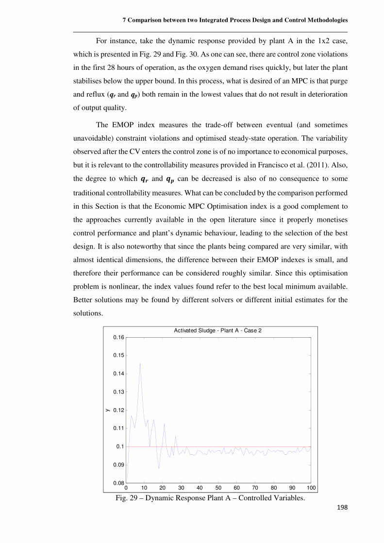
7 Comparison between two Integrated Process Design and Control Methodologies
198
For instance, take the dynamic response provided by plant A in the 1x2 case,
which is presented in Fig. 29 and Fig. 30. As one can see, there are control zone violations
in the first 28 hours of operation, as the oxygen demand rises quickly, but later the plant
stabilises below the upper bound. In this process, what is desired of an MPC is that purge
and reflux (qr and qp) both remain in the lowest values that do not result in deterioration
of output quality.
The EMOP index measures the trade-off between eventual (and sometimes
unavoidable) constraint violations and optimised steady-state operation. The variability
observed after the CV enters the control zone is of no importance to economical purposes,
but it is relevant to the controllability measures provided in Francisco et al. (2011). Also,
the degree to which �T and �Y can be decreased is also of no consequence to some
traditional controllability measures. What can be concluded by the comparison performed
in this Section is that the Economic MPC Optimisation index is a good complement to
the approaches currently available in the open literature since it properly monetises
control performance and plant’s dynamic behaviour, leading to the selection of the best
design. It is also noteworthy that since the plants being compared are very similar, with
almost identical dimensions, the difference between their EMOP indexes is small, and
therefore their performance can be considered roughly similar. Since this optimisation
problem is nonlinear, the index values found refer to the best local minimum available.
Better solutions may be found by different solvers or different initial estimates for the
solutions.
Fig. 29 – Dynamic Response Plant A – Controlled Variables.
0 10 20 30 40 50 60 70 80 90 1000.08
0.09
0.1
0.11
0.12
0.13
0.14
0.15
0.16
y
Activated Sludge - Plant A - Case 2
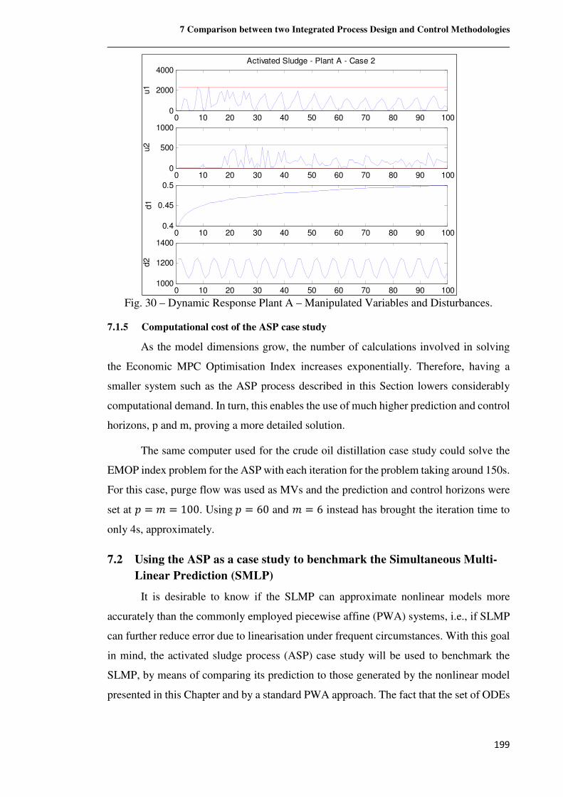
7 Comparison between two Integrated Process Design and Control Methodologies
199
Fig. 30 – Dynamic Response Plant A – Manipulated Variables and Disturbances.
7.1.5 Computational cost of the ASP case study
As the model dimensions grow, the number of calculations involved in solving
the Economic MPC Optimisation Index increases exponentially. Therefore, having a
smaller system such as the ASP process described in this Section lowers considerably
computational demand. In turn, this enables the use of much higher prediction and control
horizons, p and m, proving a more detailed solution.
The same computer used for the crude oil distillation case study could solve the
EMOP index problem for the ASP with each iteration for the problem taking around 150s.
For this case, purge flow was used as MVs and the prediction and control horizons were
set at � = � = 100. Using� = 60 and � = 6 instead has brought the iteration time to
only 4s, approximately.
7.2 Using the ASP as a case study to benchmark the Simultaneous Multi-
Linear Prediction (SMLP)
It is desirable to know if the SLMP can approximate nonlinear models more
accurately than the commonly employed piecewise affine (PWA) systems, i.e., if SLMP
can further reduce error due to linearisation under frequent circumstances. With this goal
in mind, the activated sludge process (ASP) case study will be used to benchmark the
SLMP, by means of comparing its prediction to those generated by the nonlinear model
presented in this Chapter and by a standard PWA approach. The fact that the set of ODEs
0 10 20 30 40 50 60 70 80 90 1000
2000
4000
u1
Activated Sludge - Plant A - Case 2
0 10 20 30 40 50 60 70 80 90 1000
500
1000
u2
0 10 20 30 40 50 60 70 80 90 1000.4
0.45
0.5
d1
0 10 20 30 40 50 60 70 80 90 1001000
1200
1400
d2
7 Comparison between two Integrated Process Design and Control Methodologies
200
is available for the ASP, and that the model is relatively simple, makes it convenient to
perform such a comparison.
The SMLP method is a particularly interesting option to consider when the
nonlinear model is unknown and the linear models must be obtained through model
identification at arbitrary states. To emulate this typical use scenario, the model matrices
(Eq. 199 to Eq. 202) were evaluated at three distinct, arbitrary states, yielding three linear
models. These models were used to generate a SMLP and a PWA system. Since these
systems consist of the same collection of linearised models and were provided with the
same initial operating point (OP), MVs and DVs, differences in the predictions are the
direct and sole result of differences in the methodologies themselves.
The PWA partition rules i.e., the boundaries of the active region of each
linearisation, were defined by the arithmetic mean between the model’s linearisation
states. Due to the multivariable nature of this control problem, a conflict may arise when
selecting the active model (the one used to update the state): a certain OP might lie inside
the validity region of different models at the same time if multiple variables are
considered. Therefore, the PWA model selection will be given by a voting system: each
variable casts a vote according to which space partition it is currently within, and the
model with more votes is going to be selected. In the case of a tie, the current model has
the preference if it is one the models with the same number of votes; otherwise, a random
selection of the new active model occurs.
7.2.1 A linearised state-space model for the ASP
The linearisation of the model presented in Eq. 199 to Eq. 202 is the starting point
of the process of obtaining an SMLP system for the ASP. The system was linearised at
M� different points and the resulting system was assembled in a state-space format, as
shown in Eq. 197 and Eq. 198. The linearised matrices are given in Eq. 199 to Eq. 202.
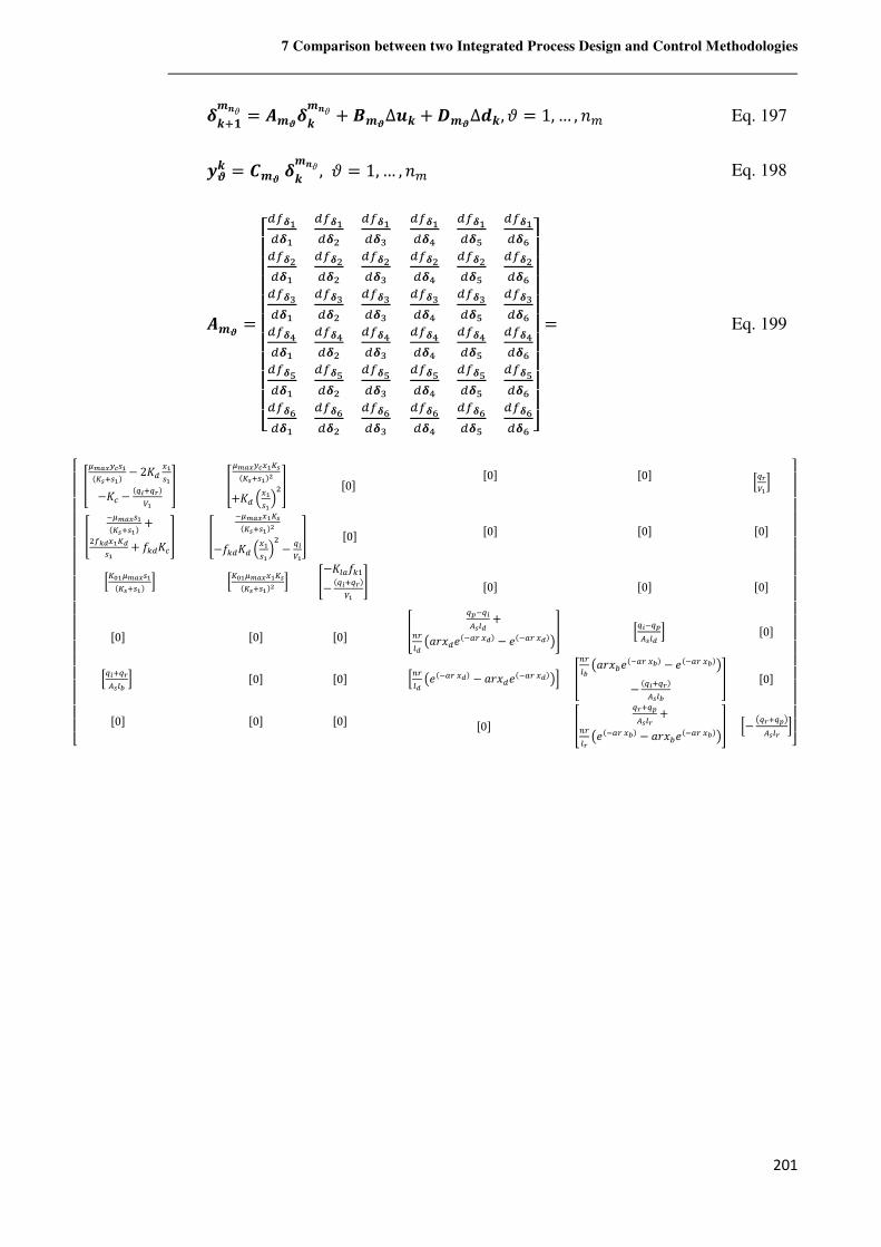
7 Comparison between two Integrated Process Design and Control Methodologies
201
�\|��hm = ����\�hm + ���∆�\ + ��∆�\,m = 1,… , M� Eq. 197
��\ = ��� �\�hm , m = 1,… , M� Eq. 198
��� =
�����������, ��,��
, ��,�p
, ��,�s
, �p,��
, �p,�p
, �p,�s
, �s,��
, �s,�p
, �s,�s
, ��,�r
, ��,�¹
, ��,�º
, �p,�r
, �p,�¹
, �p,�º
, �s,�r
, �s,�¹
, �s,�º
, �r,��
, �r,�p
, �r,�s
, �¹,��
, �¹,�p
, �¹,�s
, �º,��
, �º,�p
, �º,�s
, �r,�r
, �r,�¹
, �r,�º
, �¹,�r
, �¹,�¹
, �¹,�º
, �º,�r
, �º,�¹
, �º,�º ��
���������= Eq. 199
���������������������� �Ö_Q�Q×��
k=¦|��m − 2A, ����
−AC −k>x|>Sm=�
� �Ö_Q�Q×��=¦k=¦|��mp+A, ÷��
��ø�� µ0·
� .Ö_Q���k=¦|��m +
� )���=��� + +(,AC
� � .Ö_Q���=¦k=¦|��mp
−+(,A, ÷����ø
�− >x=�� µ0·
>=t�Ö_Q���k=¦|��m C >=t�Ö_Q���=¦
k=¦|��mp C 7−A)?+(�− k>x|>Sm=� :
µ0· µ0· >>S=�Cµ0· µ0· µ0·
µ0· µ0· µ0·
µ0· µ0· µ0·
>>x|>Sñ¦)Ï C µ0· µ0·
µ0· µ0· µ0·
� >+.>xñ¦)� +
*H)� Ô~�u,"k.?H��m − "k.?H��mÖ� >>x.>+ñ¦)� C µ0·
>*H)� Ô"k.?H��m − ~�u,"k.?H��mÖC �*H)Ï Ô~�uG"k.?H�Ïm − "k.?H�ÏmÖ− k>x|>Sm
ñ¦)Ï� µ0·
µ0· � >S|>+ñ¦)S +
*H)S Ô"k.?H�Ïm − ~�uG"k.?H�ÏmÖ� >− Ô>S|>+Ö
ñ¦)S C����������������������
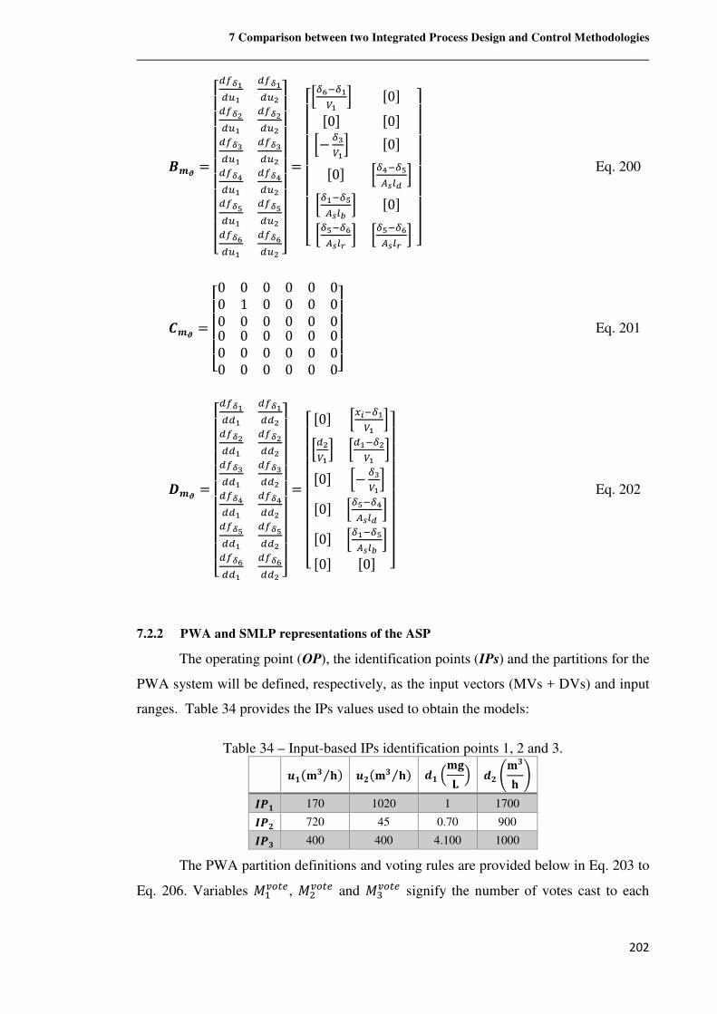
7 Comparison between two Integrated Process Design and Control Methodologies
202
��� =
�����������, �,P�
, Õ�,Pp
, Õp,P�
, Õp,Pp
, Õs,P�
, Õs,Pp
, Õr,P�
, Õr,Pp
, Õ¹,P�
, Õ¹,Pp
, Õº,P�
, պ,Pp ��
���������=
����������>Ժ.�
=� C µ0·µ0· µ0·>− Ôs=�C µ0·µ0· >Ôr.Ô¹
ñ¦)� C>Ô�.Ô¹ñ¦)Ï C µ0·>Ô¹.Ôºñ¦)S C >Ô¹.Ôº
ñ¦)S C ���������� Eq. 200
��� =
������0 0 00 1 00 0 0
0 0 00 0 00 0 0
0 0 00 0 00 0 0
0 0 00 0 00 0 0���
��� Eq. 201
�� =
�����������, �,,�
, Õ�,,p
, Õp,,�
, Õp,,p
, Õs,,�
, Õs,,p
, Õr,,�
, Õr,,p
, Õ¹,,�
, Õ¹,,p
, Õº,,�
, պ,,p ��
���������=
���������� µ0· >�x.Ô�
=� C>,p=�C >,�.Ôp=� C
µ0· >− Ôs=�C
µ0· >Ô¹.Ôrñ¦)� C
µ0· >Ô�.Ô¹ñ¦)Ï C
µ0· µ0· ���������� Eq. 202
7.2.2 PWA and SMLP representations of the ASP
The operating point (OP), the identification points (IPs) and the partitions for the
PWA system will be defined, respectively, as the input vectors (MVs + DVs) and input
ranges. Table 34 provides the IPs values used to obtain the models:
Table 34 – Input-based IPs identification points 1, 2 and 3.
��k4' Æ⁄ m � k4' Æ⁄ m �� ÷4ØÎ ø � I4'Æ J
�R� 170 1020 1 1700
�R 720 45 0.70 900
�R' 400 400 4.100 1000
The PWA partition definitions and voting rules are provided below in Eq. 203 to
Eq. 206. Variables I�JK@L, I�JK@L and IWJK@L signify the number of votes cast to each
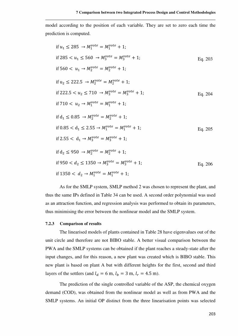
7 Comparison between two Integrated Process Design and Control Methodologies
203
model according to the position of each variable. They are set to zero each time the
prediction is computed.
iff� ≤ 285 → I�JK@L = I�JK@L + 1;
if285 < f� ≤ 560 → IWJK@L = IWJK@L + 1;
if560 < f� → I�JK@L = I�JK@L + 1; Eq. 203
ifu� ≤ 222.5 → I�JK@L = I�JK@L + 1;
if222.5 < f� ≤ 710 → IWJK@L = IWJK@L + 1;
if710 < f� → I�JK@L = I�JK@L + 1; Eq. 204
ifd� ≤ 0.85 → I�JK@L = I�JK@L + 1;
if0.85 < d� ≤ 2.55 → I�JK@L = I�JK@L + 1;
if2.55 < d� → IWJK@L = IWJK@L + 1; Eq. 205
ifd� ≤ 950 → I�JK@L = I�JK@L + 1;
if950 < ë� ≤ 1350 → IWJK@L = IWJK@L + 1;
if1350 < ë� → I�JK@L = I�JK@L + 1; Eq. 206
As for the SMLP system, SMLP method 2 was chosen to represent the plant, and
thus the same IPs defined in Table 34 can be used. A second order polynomial was used
as an attraction function, and regression analysis was performed to obtain its parameters,
thus minimising the error between the nonlinear model and the SMLP system.
7.2.3 Comparison of results
The linearised models of plants contained in Table 28 have eigenvalues out of the
unit circle and therefore are not BIBO stable. A better visual comparison between the
PWA and the SMLP systems can be obtained if the plant reaches a steady-state after the
input changes, and for this reason, a new plant was created which is BIBO stable. This
new plant is based on plant A but with different heights for the first, second and third
layers of the settlers (and F, = 6m, FG = 3m, FH = 4.5m).
The prediction of the single controlled variable of the ASP, the chemical oxygen
demand (COD), was obtained from the nonlinear model as well as from PWA and the
SMLP systems. An initial OP distinct from the three linearisation points was selected
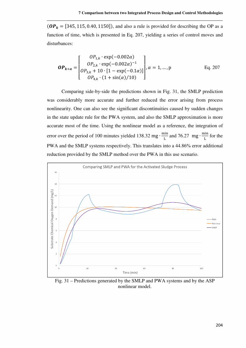
7 Comparison between two Integrated Process Design and Control Methodologies
204
k±R\ = µ345, 115, 0.40, 1150·m, and also a rule is provided for describing the OP as a
function of time, which is presented in Eq. 207, yielding a series of control moves and
disturbances:
±R\|G = ����� �d�,( ∙ expk−0.002�m
�d�,( ∙ expk−0.002�m.��dW,( + 10 ∙ µ1 − expk−0.1�m·�dv,( ∙ k1 + sink�m 10⁄ m ���
�� , � = 1,… ,p Eq. 207
Comparing side-by-side the predictions shown in Fig. 31, the SMLP prediction
was considerably more accurate and further reduced the error arising from process
nonlinearity. One can also see the significant discontinuities caused by sudden changes
in the state update rule for the PWA system, and also the SMLP approximation is more
accurate most of the time. Using the nonlinear model as a reference, the integration of
error over the period of 100 minutes yielded 138.32 mg ∙ �¬ý� and 76.27 mg ∙ �¬ý� for the
PWA and the SMLP systems respectively. This translates into a 44.86% error additional
reduction provided by the SMLP method over the PWA in this use scenario.
Fig. 31 – Predictions generated by the SMLP and PWA systems and by the ASP
nonlinear model.
7 Comparison between two Integrated Process Design and Control Methodologies
205
7.3 Final considerations about the Simultaneous Multi-Linear Prediction
method
The Simultaneous Multi-Linear Prediction (SMLP) method becomes an
interesting option when it is desired to obtain linear approximations of an unknown model
relying just on its numerical output. Moreover, the SMLP is recommended when the
number of available linearisations (sub-models) is limited but the expected operational
range is considerably wide. Thus, the SMLP brings performance improvements in some
frequent and important situations: when commercial, closed source dynamic simulation
packages are to be used for designing new plants, or when an existing plant is to be
modelled for MPC. The models show that the SMLP is able to greatly reduce the inherent
error incurred when using linearised models. It was shown that SMLP systems can be
applied in the fields of control, dynamic analysis and, as demonstrated in this Thesis,
integrated process design and control.
The main alternative to using an SMLP system would be a multi-model PWA
system. But for the typical SMLP use scenario, this may not be as good an option. The
issue is that switching the state update rules based on arbitrary, fixed thresholds may not
improve the quality of the multi-model prediction. This is true because a linear sub-model
of a piecewise affine system might not be more accurate than the rest in the entirety of its
region, i.e., there is no guarantee of obtaining an optimal partition. But even optimal
partitions can sometimes be a problem. Sudden and possibly drastic model transitions
may happen as the OP crosses a threshold. This issue is normally minimised by the
introduction of restrictions to obtain smoother transitions between the region boundaries,
but this reduces the fidelity of the approximation. Avoiding this trade-off, the use of
SMLP shifts the priority among sub-models continuously, without the need for
boundaries as a means to achieve a more faithful reproduction of the nonlinear model. No
threshold or partition rule is used and changes in the output update equation are likely to
be smoother. The SMLP regression analysis is unconstrained and solely focused on
reducing model mismatch. Also, the SMLP method does not require the use of mixed-
integer linear programming (MILP), allowing the use of faster optimisation algorithms.
SMLP systems can be used to evaluate expected flowsheet control performance
for integrated process design and control. In the case study provided, an SMLP system
was assembled to predict the dynamic behaviour of a crude oil distillation plant. This
provided the basis successfully for an application of the Economic MPC optimisation
(EMOP) index presented in Strutzel and Bogle (2016). Hence, by using the EMOP index

7 Comparison between two Integrated Process Design and Control Methodologies
206
together with the SMLP, the former became more precise and accurate in its analysis of
the economic impact of the MPC control effort.
8 Conclusions
207
8 Conclusions
This Thesis presents a novel methodology for integrated design and control of
chemical processes, the Economic MPC Optimisation (EMOP) index. It is used to
economically assessing flowsheet designs from the standpoint of zone constrained MPC
with single layer economic optimisation, whose consequences on optimal plant design
had not yet been explored at the time of writing. It is also a suitable ‘Controllability
Analysis’ approach to address industrial-scale, highly complexes systems, with special
emphasis on petroleum refining processes.
The EMOP index uses knowledge of process economics to indicate the differences
in expected revenue (or operating expenses) between candidate process designs. For this
goal, the weighting parameters in the cost function in EMOP must be representative of
the real operating conditions, and a careful selection of operation scenarios must be done
based on expected disturbances and price changes of raw materials, products and energy.
Assessing the effects of measured, modelled disturbances such as feed composition
changes is an important part of the methodology, being precisely the kind of disturbance
MPC controllers can successfully deal with. Hence, defining the scenarios for the EMOP
index evaluation is a key aspect of the analysis, requiring knowledge of both the
challenges faced during operation and the marketplace.
The fact that the EMOP cost function slightly resembles MPC cost function may
be confusing to some readers. Hence, it is important to point out that the closed-loop
behaviour was not investigated in this Thesis, which instead dealt with the issue of state
reachability constrained by zone control and disturbances, where the optimal steady-state
is defined by process economics. The option of not investigating closed-loop behaviour
was based on the desire of avoiding the generality loss that would occur if concerns such
as the choice of MPC algorithm and the selection of tuning parameters were incorporated
in the EMOP method. It is usually the flowsheet design rather than the MPC algorithm
that limits economic performance, and hence the focus was placed solely on the open-
loop behaviour. Hence, the EMOP isolates the contribution of each flowsheet’s
characteristics to an expected economic performance from other facts. A downside of this
decision is that some advances in MPC theory, such as guaranteed closed-loop stability,
8 Conclusions
208
could not be incorporated into the EMOP methodology. Assessing closed-loop steady-
states instead of open-loop could lead to the selection of plants which are not stable but
are stabilisable or controllable. The optimal operating points for such plants are likely to
lie closer to the active restrictions, and profitability could thus be higher, but the operation
could become impractical even with small malfunctions of the control system.
The other unique contribution presented in this Thesis is the Simultaneous Multi-
Linear Prediction (SMLP) method, a representation of dynamic systems composed of
multiple linear state-space models that can approximate nonlinear models or existing
plants. Strong evidence was given that the SMLP can reduce the error greatly inherently
possessed by linearisations while keeping its advantages. An important feature of SMLP
systems is that they can be built without being based on an explicit set of equations based
on first-principles. Only the numerical output of the nonlinear model (or real-world plant)
is required, differentiating the SMLP from competing approaches.
A comparison between a PieceWise Affine system (a standard multi-model
formulation) and the SMLP showed that the later provided an accuracy gain of 44.86%,
using the nonlinear model as a reference. Future work could involve the inclusion of
logical variables in the SMLP state update equations, which is an element found in the
formulations belonging to the linear hybrid framework. This would be useful to represent
complications such as saturation functions, discrete inputs, qualitative outputs, bilinear
systems and finite state machines, which are important in many processes.
It is also important to discuss openly the weaknesses of the EMOP/SMLP
framework. First of all, the large-scale case study presented in Chapter 6 was based on a
simulation that ran on a commercial, closed-source software. Such simulators are
expensive, and often the full license required to enable all the software capabilities is not
available. Furthermore, it is already a daunting task to assemble a working steady-state
simulation for a full plant and obtain consistent results. Using the dynamic mode greatly
complicates matters and, to the author’s knowledge, many design teams are satisfied with
a good steady-state simulation. The main incentive behind the development of dynamic
models in recent years has been providing training platforms for operators. In this case,
the dynamic simulation is linked to the control system and its user interface, generating a
high-fidelity environment where the operators can be prepared to perform their duties.
This opens up an interesting possibility for the EMOP index and the SMLP, which is to

8 Conclusions
209
build the models alongside the training platform, so the costs of dynamic modelling are
shared between these two activities.
Another issue encountered while building SMLP systems was a considerable time
necessary to perform the step identification and generate linear sub-models at several IPs.
A semi-automatic routine was later developed to this end, but all sub-models had to be
inspected for consistency by a person, one by one. During this process, it was found out
that a model can have an excellent fit to data scores, i.e., its output may match the
identification data perfectly, and still be far from accurate, providing very poor results
with any other input.
In my opinion, future work in the IPDCF should prioritise the multivariable
control problem, with the aim of yielding global solutions that take every variable into
account. Also present in future work should be the concern for the monetisation of control
performance, i.e., providing a clear estimate of the gains brought on by improved design.
To this end, embedding zone-constrained MPC control goal formulations is a natural
choice, especially since it is the de facto standard in the chemical industry. The ever-
growing computing power and software tools available to researchers will enable
increasingly complex first-principles or hybrid models to be built. Such models can be
used to investigate robust closed-loop performance in face of challenges such as steady-
state multiplicity, recycles, and interactions between control layers, and integration with
real-time optimisation algorithms. A plant thus projected will be truly optimised both
from the economic, operability and sustainability standpoints. I believe the way forward
should include partnerships and deep cooperation between academic institutions,
automation/process software vendors, projecting and chemical companies, which has not
been happening frequently enough. There is much to be gain from such cooperation since
hardly any of these players alone has all the pieces necessary to solve the puzzle of
designing the interconnected and smart chemical plant of the 21st century.
Future work concerning the SMLP may involve uniting it with the Linear Hybrid
Systems framework. The update equations of the SMLP’s multiple simultaneous sub-
states may be adapted to present switching behaviour, with partitions valid over regions
of the input space. Also, the update equations may be formulated with logical variables
to represent other complications of the chemical process. Also, the degradation functions
may be changed to ascribe some weight to past OP coordinates. This could act as a filter
to the rate of change between sub-model weights in the main output prediction.
References
210
References
Adetola V, Guay M. Integration of real time optimization and model predictive control. Journal of Process Control 2010;20:125–33.
Adi VSK, Chang CT. Two-tier search strategy to identify nominal operating conditions for maximum flexibility. Ind Eng Chem Res 2011;50:10707–16.
Alfani F, Carberry JJ. Chim. Ind. (Milan) 1970;52:1192.
Alhammadi H, Romagnoli J. Process Design and Operation: Incorporating Environmental, Profitability, Heat Integration and Controllability Considerations. The Integration of Process Design and Control 2004;17:264-306.
Allgöwer F, Badgwell T, Qin J, Rawlings J, Wright S. Nonlinear predictive control and moving horizon estimation – An introductory overview. P. Frank (ed.), Advances in Control, Highlights of ECC’99, Springer, London, 391–449.
Altimari P, Bildea C. Integrated design and control of plantwide systems coupling exothermic and endothermic reactions. Comput Chem Eng 2009;33:911–23.
Alvarado-Morales M, Hamid M, Sin G, Gernaey K, Woodley J, Gani R. A model-based methodology for simultaneous design and control of a bioethanol production process. Comput Chem Eng 2010;23(12):2043–61.
Alvarez H. Introducción al diseno simultáneo de proceso y control. Colombia: Académica Espanola; 2012.
Alvarez L. Tesis de Maestría en Ingeniería Química Metodología para el diseno˜ de control total de planta Tesis de Maestría en Ingeniería Química. Universidad Nacional de Colombia-Medellín; 2008.
Alvarez LA, Francischinelli EM, Santoro BF, Odloak D. Stable model predictive control for integrating systems with optimizing targets. Ind Eng Chem Res 2009;48(20):9141-50.
Angeli D, Amrit R, Rawlings JB. On Average Performance and Stability of Economic Model Predictive Control. IEEE Trans Autom Control 2012;57(7):1615–26.
Angira R, Alladwar S. Optimisation of dynamic systems: A trigonometric differential evolution approach. Comput Chem Eng 2007;31:1055–63.
Angira R, Babu BV. Optimisation of process synthesis and design problems: A modified differential evolution approach. Chem Eng Sci 2006;61:4707–21.
Angira R. Evolutionary computation for optimisation of selected nonlinear chemical processes [PhD Thesis]. Birla Institute of Technology & Science 2005, Pilani.
Asteasuain M, Bandoni A, Sarmoria C, Brandolin A. Simultaneous process and control system design for grade transition in styrene polymerization. Chem Eng Sci 2006;61:3362–78.
Asteasuain M, Brandolin A, Sarmoria C, Bandoni A. Integrated process and control system design of polymerization reactors under uncertainty. Optimal grade transition operation. In: 2nd Mercosur congress on chemical engineering. 4th Mercosur congress on process systems engineering; 2005.
Asteasuain M, Sarmoria C, Brandolin A, Bandoni A. Integration of control aspects and uncertainty in the process design of polymerization reactors. Chem Eng J 2007;131:135–44.
Babu BV, Angira R. Modified differential evolution for optimisation of nonlinear chemical processes. Comput Chem Eng 2006;30:989–1002.
Baccelli F, Cohen G, Olsder G, Quadrat J. Synchronization and Linearity. Wiley, 1992.
Bahakim S, Ricardez-Sandoval L. Simultaneous design and MPC-based control for dynamic systems under uncertainty: a stochastic approach. Comput Chem Eng 2014;63(17):66–81.
Bahri P, Bandoni A, Romagnoli J. Effect of disturbances in optimising control: the steady state open-loop back-off problem. AIChE J 1996b;42:983–94
References
211
Bahri P. PhD Thesis A new integrated approach for operability analysis of chemical plants PhD Thesis. Sydney: University of Sydney; 1996.
Bahri PA, Bandoni JA, Barton GW, Romagnoli JA. Back-off calculations in optimising control: a dynamic approach. Comput Chem Eng 1995;19:699-708.
Bahri PA, Bandoni JA, Romagnoli JA. Integrated flexibility and Controllability Analysis in design of chemical processes. AIChE J 1997;43:997–1015.
Bahri PA, Bandoni JA, Romagnoli JA. Operability assessment in chemical plants. Comput Chem Eng 1996a;S20:S787–92.
Baker R, Swartz C. Interior point solution of integrated plant and control design problems with embedded MPC. In: AIChE annual meeting; 2006. p. 12–7.
Bandoni JA, Romagnoli JA, Barton G. On optimizing control and the effect of disturbances: calculation of the open loop backoffs. Comput Chem Eng 1994;18S:105S–9S.
Bansal V, Perkins J, Pistikopoulos E. A case study in simultaneous design and control using rigorous, mixed-integer dynamic optimisation models. Ind Eng Chem Res 2002b;41(4):760–78.
Bansal V, Perkins J, Pistikopoulos E. Flexibility analysis and design of dynamic processes with stochastic parameters. Comput Chem Eng 1998;22S:S817–20.
Bansal V, Perkins JD, Pistikopoulos E, Ross R, van Schijndel JMG. Simulta-neous design and control optimisation under uncertainty. Comput Chem Eng 2000a;24:261–6.
Bansal V, Perkins JD, Pistikopoulos E. Flexibility analysis and design of linear systems by parametric programming. AIChE J 2000b;46:335.
Bansal V, Perkins JD, Pistikopoulos E. Flexibility analysis and design using a parametric programming framework. AIChE J 2002a;48(12):2851–68.
Bansal V, Perkins JD, Pistikopoulos EN. A case study in simultaneous design and control using rigorous, mixed-integer dynamic optimisation models. Ind Eng Chem Res 2002;41:760–78.
Bansal V, Sakizlis V, Ross R, Perkins JD, Pistikopoulos EN. New algorithms for mixed integer dynamic optimisation. Comput Chem Eng 2003;27:647–68.
Barton G, Padley M, Perkins J. Incorporating operability measures into the process synthesis stage of design. In: Proceedings of IFAC workshop on interactions between process design and process control. London: Pergamon Press; 1992. p. 95–8.
Bemporad A, Garulli A, Paoletti S, Vicino A. A bounded-error approach to piecewise affine system identification. IEEE Trans Autom Control 2005;50(10):1567–80.
Bemporad A, Morari M. Robust model predictive control: A survey, Lecture Notes in Control and Information Sciences 1999;245:207–226.
Bemporad A, Morari M: Control of systems integrating logic, dynamics, and constraints. Automatica 1999, 35(3):407–27.
Bildea C, Dimian A, Cruz S, Iedema P. Design of tubular reactors in recycle systems. Comput Chem Eng 2004;28(1–2):63–72.
Bildea C, Dimian A. Fixing flow rates in recycle systems: Luyben’s rule revisited. Ind Eng Chem Res 2003;42:4578.
Biss D, Perkins JD. Application of input-output Controllability Analysis to chemical processes. Proc ECC 1993, Groningen, Netherlands, 1056-1059.
Blanco A, Bandoni A. Interaction between process design and process operability of chemical processes: an eigenvalue optimisation approach. Comput Chem Eng 2003;27(8–9):1291–301.
Brambilla A. Distillation Control & Optimization: Operation Fundamentals through Software Control. McGraw-Hill 2014. ISBN-13: 978-0071820684.
Brengel DD, Seider W. Coordinated design and control optimization of nonlinear processes, Chem Eng Com 1992;16:861–86.
Bristol EH. On a new measure of interaction for multivariable process control. IEEE Trans Autom Control 1966;11:186–93.
References
212
Calderón C, Alzate A, Gómez L, Alvarez H. State Controllability Analysis and re-design for a wastewater treatment plant. In: Mediterranean conference on control and automation; 2012a.
Calderón C, Gómez L, Alvarez H. Nonlinear state space controllability: set theory vs differential geometry. In: Congreso Latinoamericano de Control Automático; 2012b.
Campo PJ, Morari M. Achievable closed-loop properties of systems under decentralized control: Conditions involving the steady-state gain. IEEE Trans. Autom. Control 1994;39:932– 43.
Campo PJ, Morari M. Robust model predictive control. Proc American Contr Conf 1987;2:1021–26.
Chang C, Li B, Liou C. Development of a generalized mixed integer nonlinear pro-gramming model for assessing and improving the operational flexibility of water network designs. Ind Eng Chem Res 2009;48(7):3496–504.
Chawankul N, Ricardez-Sandoval LA, Budman H, Douglas PL. Integration of Design and Control: A Robust Control Approach Using MPC. The Canadian Journal of Chemical Engineering 2007;85(4):433–46.
Chen H, Allgower F. A quasi-infinite horizon nonlinear model predictive control scheme with guaranteed stability. Automatica 1998;34(10):1205–17.
Cheng Y, Yu Ch. Effects of process design on recycle dynamics and its implication to control structure selection. Ind Eng Chem Res 2003;42:4348–65.
Christofides PD, Scattolini R, de la Peña DM, Liu J. Distributed model predictive control: A tutorial review and future research directions. Comput Chem Eng 2013;51:21–41.
Christophersen FJ. Optimal Control and Analysis for Constrained Piecewise Affine Systems. Dissertation ETH Zurich No. 16807.
Cottle RW, Pang JS, Stone RE. The Linear Complementarity Problem, Academic Press, Cambridge, 1992.
Cuninghame-Green R. Minimax Algebra. Springer, 1979.
Cutler CR. Dynamic Matrix Control: An Optimal Multivariable Control Algorithm with Consraints. Ph.D. Thesis, U. of Houston 1983.
Cutler CR, Ramaker BL. Dynamic Matrix Control-A Computer Control Algorithm. AIChE 86th National Meeting 1979, Houston, TX.
De Schutter B, Van den Boom T. On model predictive control for max-min-plus-scaling discrete event systems. Automatica 2001, 37(7):1049–56.
De Wal MV, Jager BD. A review of methods for input/output selection. Automatica 2001;37:487–510.
Denn MM, Lavie R. Dynamics of plants with recycle. Chem Eng J 1982;24:55–9. Dimian A, Groenendijk A, Kersten S, Iedema P. Effect of recycle interactions on
Dimian AC, Groenendijk AJ, Kersten SRA, Iedema PD. Effect of Recycle Interactions on Dynamics and Control of Complex Plants. Comput Chem Eng 1997;21:291–96.
Dimitriadis V, Pistikopoulos E. Flexibility analysis of dynamic systems. Ind Eng Chem Res 1995;34(12):1451–4462.
Dominguez D, Revollar S, Francisco M, Lamanna R, Vega P. Simultaneous synthesis and integrated design of chemical processes using IMC PID tuning methods. In: International conference on chemical and process engineering (IcheaP); 2009.
Dougherty D, Cooper D. A practical multiple model adaptive strategy for single-loop MPC. Control Engineering Practice 2003:11:141–159.
Downs J, Moore C. Steady-State Gain Analysis for Azeotropic Distillation. Proceedings of the Joint American Control Conference, 1981; Paper WP-7.
Downs JJ, Vogel EF. A plant wide industrial process control problem. American Institute of Chemical Engineering Annual mtg. Chicago, USA, 1990.
E. Sontag, “Nonlinear regulation: The piecewise linear approach,” IEEE Trans Autom Control, vol. 26, no. 2, pp. 346–358, 1981.
Edgar TF. Control and operations: when does controllability equal profitability? Comput Chem Eng 2004;29:41–49.
References
213
Egea JA, Vries D, Alonso A, Banga JR. Global optimisation for integrated design and control of computationally expensive process models. Ind Eng Chem Res 2007;46:9148–57.
Ekawati E, Bahri P. Integration of output controllability index within dynamic operability framework in process system design. J Process Contr 2003;13: 717–27.
Ekawati E. PhD Thesis The development of systematic controllability assessment for process control designs PhD Thesis. School of Engineering Science, Murdoch University; 2003.
Elliott T, Luyben WL. Capacity-based approach for the quantitative assessment of process controllability during the conceptual design stage. Ind Eng Chem Res 1995;34:3907–15.
Elliott T, Luyben WL. Quantitative assessment of controllability during the design of a ternary system with two recycle streams. Ind Eng Chem Res 1996;35: 3470–9.
Exler O, Antelo LT, Egea JA, Alonso AA, Banga JR. A tabu search-based algorithm for mixed-integer nonlinear problems and its application to integrated process and control system design. Comput Chem Eng 2008;32:1877–91.
Farina L, Rinaldi S. Positive Linear Systems: Theory and Applications. Wiley 2000.
Ferrari-Trecate G, Muselli M, Liberati D, Morari M. A clustering technique for the identification of piecewise affine systems. Automatica 2003, 39(2):205–17.
Findeisen R, Allgöwer F. An introduction to nonlinear model predictive control. 21st Benelux Meeting on Systems and Control 11, 119-141, 2002.
Flores-Tlacuahuac A, Biegler L. Integrated control and process design during optimal polymer grade transition operations. Comput Chem Eng 2008;32: 2823–37.
Flores-Tlacuahuac A, Biegler L. Simultaneous mixed-integer dynamic optimisation for integrated design and control. Comput Chem Eng 2007;31:588–600.
Francisco M, Revollar S, Vega P, Lamanna R. Simultaneous synthesis, design and control of processes using model predictive control. In: Proceedings of international symposium on advanced control of chemical processes (Adchem); 2009.
Francisco M, Vega P, Alvarez H. Robust integrated design of process with terminal penalty model predictive controllers. Ind Eng Chem Res 2011;89:1011−24.
Francisco M. PhD Tesis Diseno simultaneo de procesos y sistemas de control predictivo mediante índices de controlabilidad basados en normas PhD Tesis. Spain: Universidad de Salamanca; 2011.
Gani R, Hytoft G, Jaksland C, Jensen A. An integrated computer aided system for integrated design of chemical processes. Comput Chem Eng 1997;21:1135–46.
Garcia CE, Morari M. Internal model control. A unifying review and some new results. Ind Eng Chem Process Des Dev 1982;21(2):308–23.
Garcia CE, Prett DM, Morari M. Model predictive control: theory and practice – a survey. Automatica 1989;25(3):335-48.
Garcia EG, Morshedi AM. Quadratic Programming Solution of Dynamic Matrix Control (QDMC). Chem Eng Com 1986;46(1-3):73-87.
Garulli A, Paoletti S, Vicino A. A survey on switched and piecewise affine system identification. 16th IFAC Symposium on System Identification 2012; The International Federation of Automatic Control.
Gareth J. An Introduction to Statistical Learning: with Applications in R. Springer, 2013:176. ISBN 978-1461471370.
Georgakis C, Uzturk D, Subramanian S, Vinson D. On the operability of continuous processes. Control Eng Pract 2003;11:859–69.
Georgiou A, Floudas C. Structural properties of large scale systems. Int J Control 1990;51(1):169–87.
Gerhard J, Monnigmann M, Marquardt W. Constructive nonlinear dynamics foundations and application to robust nonlinear control. In: Meurer T, Graichen K, Gilles ED, editors. Control and observer design for nonlinear finite and infinite dimensional systems, vol. 322. Berlin: Springer; 2005. p. 165–82.
González AH, Odloak D. A stable MPC with zone control. Journal of Process Control 2009;19(1):110–122.
References
214
Gonzalez AH, Perez JM, Odloak D. Infinite horizon MPC with non-minimal state space feedback. J Proc Control 2009;19:473–81.
Gopinath, R., Bequette, B. W., Roy, R. J., Kaufman, H., & Yu, C. Issues in the design ofa multirate model-based controller for a nonlinear drug infusion system. Biotechnology Progress 1995;11:318–32.
Gouvêa MT, Odloak D. One-layer real time optimization of LPG production in the FCC unit: Procedure, advantages and disadvantages. Comput Chem Eng 1998;22:191–98.
Grosch R, Mönnigmann M, Marquardt W. Integrated design and control for robust performance: application to an MSMPR crystallizer. J Process Contr 2008;18:173–88.
Grosdidier P, Morari M, Holt BR. Closed-Loop properties from Steady-State Gain Information. Ind Eng Chem Fundam 1985;24:221–35.
Grosman B, Dassau E, Zisser HC, Jovanovič L, Doyle III FJ. Zone Model Predictive Control: A Strategy to Minimize Hyper- and Hypoglycemic Events. Journal of Diabetes Science and Technology 2010;4(4).
Grossmann IE, Floudas C. Active constraint strategy for flexibility analysis of chemical processes. Comput Chem Eng 1987;11(6):675–93.
Grossmann IE, Halemane KP, Swaney RE. Optimization Strategies for Flexible Chemical Processes. Comput Chem Eng 1983;7(4):439–62.
Grossmann IE, Morari M. Operability, resiliency and flexibility – process design objectives for a changing world. In: Westerberg AW, Chien HH, editors. Proceedings of 2nd international conference on foundations of computer-aided process design; 1984. p. 931.
Grossmann IE, Straub DA. Recent Developments in the Evaluation and Optimization of Flexible Chemical Processes. In: Puigjaner L, Espuna A, editors. Computer-oriented process engineering, vol. 10. Amsterdam: Elsevier; 1991. p. 49–59.
Guerra I, Lamanna R, Revollar S. An activated-sludge-process application of integrated design and predictive control with instantaneous linearization. In: IEEE Mediterranean conference on control and automation; 2012.
Gutierrez G, Ricardez-Sandoval LA, Budman H, Prada C. An MPC-based control structure selection approach for simultaneous process and control design. Comput Chem Eng 2013., http://dx.doi.org/10.1016/j.compchemeng.2013.08.014.
Gutiérrez G, Vega P. Integrated design of activated sludge process taking into account the closed loop controllability. In: Proceedings of the ESCAPE, 10; 2000. p. 63–9.
Gutierrez G. PhD Tesis Diseno˜ integrado y síntesis de procesos aplicada al proceso de fangos activados PhD Tesis. Spain: Universidad de Valladolid; 2000.
Halemane KP, Grossmann IE. Optimal process design under uncertainty. AIChE J 1983;29:425–33.
Hamid M, Kamaruddin bin Abd. Model-based integrated process design and controller design of chemical processes. Ph.D. Thesis; 2011.
Hamid M, Sin G, Gani R. Integration of process design and controller design for chemical processes using model based methodology. Comput Chem Eng 2010;34:683–99.
Hautus M. Controllability and stabilizability of sampled systems. IEEE Trans Autom Control 1972;17(4):528–531.
Heemels WPMH, De Schutter B, Bemporad A. Equivalence of hybrid dynamical models. Automatica 2001, 37(7):1085–91.
Heemels WPMH, Schumacher JM, Weiland S. Linear complementarity systems. SIAM J Appl Math 2000, 60(4):1234–69.
Heidarinejad M, Liu J, Christofides PD. Economic model predictive control of nonlinear process systems using Lyapunov techniques. AIChE Journal 2012;58(3):855-70.
Hermann R, Krener AJ. Nonlinear controllability and observability. IEEE Trans Autom Control 1977:5.
Holt B, Morari M. Design of resilient processing plants—V: The effect of deadtime on dynamic resilience. Chem Eng Sci 1985a;40(7):1229–37.
References
215
Holt B, Morari M. Design of resilient processing plants—VI. The effect of right-half-plane zeros on dynamic resilience. Chem Eng Sci 1985b;40(1):59–74.
Hopkins L, Lant P, Newell B. Output structural controllability: a tool for integrated process design and control. J Process Contr 1998;8(1):57–68.
Iman RL, Helton JC. An Investigation of Uncertainty and Sensitivity Analysis Techniques for Computer Models. Risk Analysis 1988;8(1):71–90.
Jacobsen E. Effect of recycle on the plant zero dynamics. Comput Chem Eng 1997;21(Suppl. 20):S279–84.
Jadbabaie A. Nonlinear Receding Horizon Control: A Control Lyapunov Function Approach. PhD thesis, California Institute of Technology, Control and Dynamical Systems, 2001.
Juloski ALj, Weiland S, Heemels WPMH. A Bayesian approach to identification of hybrid systems. IEEE Trans Autom Control 2005;50(10):1520–33.
Kalman RE, Falb PL. Arbib MA. Topic in Mathematical System Theory, MacGraw-Hill Book Company, New York, 1969.
Kalman RE. A new approach to linear filtering and prediction problems. Journal of Basic Engineering 1960;82 (1):35–45.
Kantner M, Primbs J. Nonlinear MPC Lower Bounds via Robust Simulation. Proceedings of the American Control Conference Albuquerque 1997, New Mexico.
Karafyllis I, Kokossis A. On a new measure for the integration of process design and control: The disturbance resiliency index. Chem Eng Sci 2002;57:873–86.
Keerthi SS, Gilbert EG. Optimal infinite-horizon feedback control laws for a general class of constrained discrete-time systems: stability and moving-horizon approximations. J. Opt. Theory and Applications 1988;57:265– 93.
Kim S, Linninger A. Integration of design and control for a large scale flowsheet. In: Pierucci S, Buzzi Ferraris G, editors. 20th European symposium on computer aided process engineering (ESCAPE-20). Ischia: Elsevier B.V.; 2010.
Kiss A, Bildea C, Dimian A, Iedema P. Design of recycle systems with parallel and consecutive reactions by nonlinear analysis. Ind Eng Chem Res 2005;44: 576–87.
Kookos IK, Perkins JD. An algorithm for simultaneous process design and control. Ind Eng Chem Res 2001;40:4079–88.
Kookos IK, Perkins JD. An algorithmic method for the selection of multivariable process control structures. J Proc Control 2002;12(1):85–99.
Kookos IK, Perkins JD. Heuristic-Based Mathematical Programming Framework for Control Structure Selection. Ind Eng Chem Res 2001;40 (9):2079–88.
Koppel LB. Input multiplicities in nonlinear multivariable control system. AIChE J 1982;28(6):935–45.
Kothare MV, Balakrishnan V, Morari M. Robust constrained model predictive control using linear matrix inequalities. Automatica 1996;32(10):1361-79.
Krstic M, I. Kanellakopoulos I, Kokotovic P. Nonlinear and Adaptive Control Design. Wiley, 1995.
Kurt E. Häggblom. Integral Controllability and Integrity for Uncertain Systems. IEEE. 2008 American Control Conference. Seattle, Washington, USA.
Kwon WH, Bruckstein AM, Kailath T. Stabilizing state-feedback design via the moving horizon method. Int. J. Control 1983;37(3):631–43.
Kwon WH, DG Byun. Receding horizon tracking control as a predictive control and its stability properties. Int. J. Control 1989;50(5):1807– 24.
Kwon WH, Pearson AE. A modified quadratic cost problem and feedback stabilization of a linear system. Automatic Control 1977;22(5):838–42.
Lakshminarayanan S. Recycle effect index: a measure to aid in control system design for recycle processes. Ind Eng Chem Res 2004;6:1499–511.
Lamanna R, Vega P, Revollar S, Alvarez H. Diseno˜ Simultáneo de Proceso y Control de una Torre Sulfitadora de Jugo de Cana˜ de Azúcar. Rev Iberoam Autom Inform Ind 2009;6(3):32–43.
References
216
Langson W, Chryssochoos I, Rakovic SV, Mayne DQ. Robust model predictive control using tubes. Automatica 2004;40(1):125–33.
Lau H, Alvarez J, Jensen K. Synthesis of Control Structure by Singular Value Analysis. AIChE J 1985;31:427.
Lee B, Kim Y, Shin D, Yoon E. A study of the evaluation of structural controllability in chemical processes. Comput Chem Eng 2001;25:85–95.
Lee JH, Morari M, Garcia CE. State-space interpretation of model predictive control. Automatica 1994;30(4):707-17.
Lenhoff A, Morari M. Design of resilient processing plants—I. Process design under consideration of dynamic aspects. Chem Eng Sci 1982;37:245–58.
Lewin DR. A simple tool for disturbance resiliency diagnosis and feed-forward control design. Comput Chem Eng 1996;20(1):13–25.
Lewin DR. Interaction of design and control. Proceedings of 7th Mediterranean conference on control and automation (MED 99), Hafia, Israel, 1999.
Li H, Gani R, Jørgensen S. Process-insights-based control structuring of an integrated distillation pilot plant. Ind Eng Chem Res 2003;42:4620–7.
Li P, Arellano-Garcia H, Wozny G. Chance constrained programming approach to process optimisation under uncertainty. Comput Chem Eng 2008;32(1–2): 25–45.
Lima F, Georgakis C, Smith J, Schnelle P, Vinson D. Operability-based determination of feasible control constraints for several high-dimensional nonsquare industrial processes. AIChE J 2010a;56(5):1249–61.
Lima F, Jia Z, Ierapetritou M, Georgakis C. Similarities and differences between the concepts of operability and flexibility: the steady-state case. AIChE J 2010b;56:702–16.
Lin X, Tade M, Newell R. Output structural controllability condition for the syn-Thesis of control systems for chemical processes. Int J Syst Sci 1991;22(1): 107–32.
Liu J, Muñoz de la Peña D, Christofides PD. Distributed model predictive control of nonlinear process systems. AIChE Journal 2009;55(5):1171-84.
Loeblein C, Perkins J. Structural design for on-line process optimisation: I. Dynamic economics of MPC. AIChE J 1999;45(5):1018–29.
Lowe GK, Zohdy MA. Modeling nonlinear systems using multiple piecewise linear equations. Nonlinear Analysis: Modelling and Control 2010;15(4):451–58.
Lu X, Li H, Duan J, Su D. Integrated design and control under uncertainty: a fuzzy modelling approach. Ind Eng Chem Res 2010;49:1312–24.
Lucia S, Finkler T, Engell S. Multi-stage nonlinear model predictive control applied to a semi-batch polymerization reactor under uncertainty. J Proc Cont 2013;23(9):1306–19.
Luo X, Zhou X, Wang S, Xu F. Zone Control with Model Predictive Control for Much Constrained States Process. Proceedings of the 31st Chinese Control Conference, July 25-27, 2012, Hefei, China.
Luyben ML, Floudas C. Analyzing the interaction of design and control–1. A multi-objective framework and application to binary distillation synthesis. Comput Chem Eng 1994a;18:933–69.
Luyben ML, Floudas C. Analyzing the interaction of design and control–2. Reactor–separator–recycle system. Comput Chem Eng 1994b;18:971–93.
Luyben ML, Luyben WL. Design and control of a complex process involving two reaction steps, three distillation columns, and two recycle streams. Ind Eng Chem Res 1996;34:3885–98.
Luyben WL, Pszalgowski KM, Schaefer MR, Siddons C. Design and control of conventional and reactive distillation processes for the production of butyl acetate. Ind Eng Chem Res 2004;43(25):8014-25.
Luyben WL. Design and control of gas-phase reactor/recycle processes with reversible exothermic reactions. Ind Eng Chem Res 2000;39:1529.
Luyben WL. Distillation Design and Control Using Aspen Simulation, 2nd Edition. Wiley 2013. ISBN: 978-1-118-41143-8.
References
217
Luyben WL. Dynamics and control of recycle systems. 1. Simple open-loop and closed-loop systems. Ind Eng Chem Res 1993a;32:466–75.
Luyben WL. Dynamics and control of recycle systems. 2. Comparison of alternative process designs. Ind Eng Chem Res 1993b;32:476–86.
Luyben WL. Dynamics and control of recycle systems. 3. Alternative process designs in a ternary system. Ind Eng Chem Res 1993c;32:1142–53.
Luyben WL. Effect of feed impurity on the design and control of a ternary two-recycle process. Ind Eng Chem Res 1999;38:3430–7.
Luyben WL. Snowball effects in reactor/separator processes with recycle. Ind Eng Chem Res 1994;33:299–305.
Lyapunov AM. The General Problem of the Stability of Motion (In Russian), Doctoral dissertation, Univ. Kharkov 1892 English translations: (1) Stability of Motion, Academic Press, New-York & London, 1966 (2) The General Problem of the Stability of Motion, (A. T. Fuller trans.) Taylor & Francis, London 1992.
Ma K, Valdés-González H, Bogle IDL. Process design in SISO systems with input multiplicity using bifurcation analysis and optimisation. J Proc Control 2010;20(3):241-47.
Mahdi Sharifzadeh. Integration of process design and control: A review. Chem Eng Res Des 2013; 91(12): 2515–49.
Malcolm A, Polan J, Zhang L, Ogunnaike BA, Linninger A. Integrating systems design and control using dynamic flexibility analysis. AIChE J 2007;53: 2048–61.
Marselle D, Morari M, Rudd D. Design of resilient processing plants. II. Design and control of energy management systems. Chem Eng Sci 1982;37:259–70.
Matallana L, Blanco A, Bandoni A. Nonlinear dynamic systems design based on the optimisation of the domain of attraction. Math Comput Model 2011;53(5–6):731–45.
McAvoy T, Braatz RD. Controllability of Processes with Large Singular Values. Ind Eng Chem Res 2003;42:6155–65.
McAvoy T, Miller R. Incorporating integrating variables into steady-state models for plantwide control analysis and design. Ind Eng Chem Res 1999;38:412–20.
Meeuse F, Deugd R, Kapteijn F, Verheijen P, Ypma S. Increasing the selectivity of the Fischer Tropsch process by periodic operation. Comput Aided Chem Eng 2001;9:699–704.
Meeuse F, Grievink J, Verheijen P, Vander M. Conceptual design of processes for structured products. In: Malone, Trainham, Carnahan, editors. Proceedings ESCAPE-5; 2000. p. 324–8.
Meeuse F, Grievink J. Optimum controllability of distributed systems based on non-equilibrium thermodynamics. In: Grievink J, Schijndel JV, editors. ESCAPE-12; 2002. p. 259–64.
Meeuse F, Grievink J. Thermodynamic controllability assessment in process synthe-sis. In: Seferlis P, Georgiadis MC, editors. The integration of process design and control. Amsterdam: Elsevier B.V.; 2004. p. 146–67.
Meeuse F. PhD Thesis On the design of chemical processes with improved control-lability characteristics PhD Thesis. Technische Universiteit Delft; 2002.
Mhaskar P, El-Farra NH, Christofides PD. Predictive control of switched nonlinear systems with scheduled mode transitions IEEE Trans Autom Control 2005:50(11):1670-80.
Mhaskar P, El-Farra NH, Christofides PD. Stabilization of nonlinear systems with state and control constraints using Lyapunov-based predictive control. Systems & Control Letters 2006;55(8):650-59.
Miranda M, Reneaume J, Meyer X, Meyer M, Szigetid F. Integrating process design and control: an application of optimal control to chemical processes. Chem Eng Process 2008;47(11):2004–18.
Mohideen MJ, Perkins JD, Pistikopoulos EN. Optimal design of dynamic systems under uncertainty. AIChE Journal 1996b;42(8):2251–72.
Mohideen MJ, Perkins JD, Pistikopoulos EN. Optimal synthesis and design of dynamic systems under uncertainty. Comput Chem Eng 1996a;20S:S895–900.
References
218
Monnigmann M, Marquardt W. Normal vectors on manifolds of critical points for parametric robustness of equilibrium solutions of ODE systems. J Nonlinear Sci 2002;12:85–112.
Monnigmann M, Marquardt W. Steady-state process optimisation with guaranteed robust stability and flexibility: application to HDA reaction section. Ind Eng Chem Res 2005;44:2737–53.
Moon J, Kim S, Linninger A. Integrated design and control under uncertainty: embedded control optimisation for plantwide processes. Comput Chem Eng 2011;35:1718–24.
Moore C. Application of SVD for the Design, Analysis, and Control of Industrial Processes. Proceedings of the American Control Conference, 1986; Paper TA-1.
Morari M, Arkun Y, Stephanopoulos G. Studies in the synthesis of control structures for chemical processes: Part I: Formulation of the problem. Process decomposition and the classification of the control tasks. Analysis of the optimizing control structures. AIChE J 1980;26(2):220–3.
Morari M, Grimm W, Oglesby M, Prosser I. Design of resilient processing plants—VII. Design of energy management system for unstable reactors—new insights. Chem Eng Sci 1985;40(2):187–98.
Morari M, Lee JH. Model predictive control. Past, present and future. Comput Chem Eng 1999;23:667-82.
Morari M, Stephanopoulos G. Studies in the synthesis of control structures for chemical processes: Part II: Structural aspects and the synthesis of alternative feasible control schemes. Analysis of the optimizing control structures. AIChE J 1980;26(2):232–46.
Morari M, Zafiriou E, Holt B. Design of resilient processing plants. New characteri-zation of the effect of RHP zeros. Chem Eng Sci 1987;42(10):2425–8.
Morari M, Zafiriou E. Robust process control. Prentice-Hall 1989.
Morari M. Design of resilient processing plants—III. A general framework for the assessment of dynamic resilience. Chem Eng Sci 1983a;38:1881.
Morari M. Flexibility and resiliency of process systems. Comput Chem Eng 1983b;7:423–437.
Morshedi AM, Cutler CR, Skovanek TA. Optimal Solution of Dynamic Matrix Control with Linear Programming Techniques (LDMC). Proc automatic Control Conf 1985;199.
Morud J, Skogestad S. The dynamic behavior of integrated plants. In: Symposium PSE’94; 1994. p. 913–8.
Munoz D, Alvarez H, Ochoa S. ¿Hacia dónde va la integración del diseno y el control del proceso? El papel de la controlabilidad de estado y el diseno bajo incer-tidumbre. In: XIII Congreso Latinoamericano de Control Automático/VI Congreso Venezolano de Automatización y Control; 2008.
Munoz D, Gerhard J, Marquardt W. A normal vector approach for integrated process and control design with uncertain model parameters and disturbances. Comput Chem Eng 2012;40:202–12.
Muske KR, Rawlings JB. Model predictive control with linear models. AIChE J 1993;39(2):262–87.
Nakada H, Takaba K, Katayama T. Identification of piecewise affine systems based on statistical clustering technique. Automatica, 41(5):905–913, 2005.
Narraway L, Perkins JD, Barton G. Interactions between process design and process control: economic analysis of process dynamics. J Process Contr 1991;1:243–50.
Narraway L, Perkins JD. Selection of process control structure based in economics. Comput Chem Eng 1994;S18:S511–5.
Narraway L, Perkins JD. Selection of process control structure based on linear dynamic economics. Ind Eng Chem Res 1993;32:2681–92.
Novak Pintaric Z, Kravanja Z. A strategy for MINLP synthesis of flexible and operable processes. Comput Chem Eng 2004;28(6–7):1105–19.
Ochoa S, Alvarez H. A methodology for the integration of process design and control in the state space. In: Proceedings of the 2nd Mercosur congress on chemical engineering and 4th Mercosur congress on process systems engineering; 2005.
Ochoa S. Master Thesis A methodology for the design-control integration in state-space Master Thesis. Medellín: National University of Colombia; 2005 [in Spanish].
Ogata K. Modern Control Engineering. Prentice Hall, 1997.
References
219
Palazoglu A, Arkun Y. A multiobjective approach to design chemical plants with robust dynamic operability characteristics. Comput Chem Eng 1986;10:567–75.
Paoletti S, Juloski A Lj. , G. Ferrari-Trecate, and R. Vidal. Identification of hybrid systems: A tutorial. European Journal of Control 2007;13(2–3):242–60.
Patel J, Uygun K, Huang Y. A path constrained method for integration of process design and control. Comput Chem Eng 2007;32:1373–84.
Perkins JD, Walsh SPK. Optimization as a tool for design/control integration. Comput Chem Eng 1996;20(4):315–23.
Pistikopoulos EN, Van Schijndel JMG. Towards the integration of process design, process control & process operability - current status & future trends. In Foundations of Computer-Aided Process Design, Snowmass, Colorado, USA, 1999.
Polak E, Yang TH. Moving horizon control of linear systems with input saturation and plant uncertainty–part 1. robustness. Int. J. Control 1993a;58(3):613–638.
Polak E, Yang TH. Moving horizon control of linear systems with input saturation and plant uncertainty–part 2. disturbance rejection and tracking. Int. J. Control 1993b;58(3):639–663.
Porfírio CR, Odloak D. Optimizing model predictive control of an industrial distillation column, Control Engineering Practice 2011;19(10):1137–46.
Psarris P, Floudas CA. Dynamic operability of MIMO systems with time delays and transmission zeroes. I. Assessment. Chem Eng Sci 1991;46(10):2691–707.
Ramirez Jimenez E, Gani R. Methodology for the design and analysis of reaction-separation systems with recycle. 1. The design perspective. Ind Eng Chem Res 2007a;46(24):8066–83.
Ramirez Jimenez E, Gani R. Methodology for the design and analysis of reaction-separation systems with recycle. 2. Design and control algorithms. Ind Eng Chem Res 2007b;46(24):8084–100.
Rashid MA, Moses OT. Nonlinear Model-based Process Control Applications in Petroleum Refining, Springer 2000.
Revollar S, Francisco M, Vega P, Lamanna R. Genetic algorithms for the synthesis and integrated design of processes using advanced control strategies. In: International symposium on distributed computing and artificial intelligence (DCAI’08). Lecture Notes on Computer Science 50/2009; 2008. p. 205–14.
Revollar S, Francisco M, Vega P, Lamanna R. Stochastic optimisation for the simultaneous synthesis and control system design of an activated sludge process. Latin Am Appl Res 2010a;40:137–46.
Revollar S, Lamanna R, Rodríguez A, Vega P, Francisco M. Integrated design methodology for improving the economics and dynamical performance of the activated sludge process. In: Ecotechnologies for wastewater treatment. Technical, envi-ronmental and economic challenges (ECOSTP); 2012.
Revollar S, Lamanna R, Vega P, Francisco M. Multiobjective genetic algorithms for the integrated design of chemical processes using advanced control techniques. In: Pierucci S, Buzzi Ferraris G, editors. Proceedings of 20th European symposium on computer aided process engineering (ESCAPE-20). Ischia: Elsevier B.V.; 2010b.
Revollar S, Rodríguez A, Lamanna R, Francisco M, Vega P. Multiobjective genetic algorithms for the simultaneous design and control of the activated sludge process. In: Proceedings of Congress of chemical and process engineering (CHISA 2010); 2010c.
Revollar S. PhD Tesis Algortimos genéticos en el diseno integrado de procesos quími-cos PhD Tesis. Venezuela: Universidad Simón Bolívar; 2011.
Reyes F, Luyben WL. Design and control of a gas-phase adiabatic tubular reactor process with liquid recycle. Ind Eng Chem Res 2001a;40(17):3762–74.
Reyes F, Luyben WL. Design and control of tubular reactor systems with both gas and liquid recycles. Ind Eng Chem Res 2001b;40(19):4089–101.
Reyes F, Luyben WL. Steady-state and dynamic effects of design alternatives in heat-exchanger/furnace/reactor processes. Ind Eng Chem Res 2000;39:3335.
Ricardez-Sandoval L, Budman H, Douglas P. Application of robust control tools to the simultaneous design and control of dynamic systems. Ind Eng Chem Res 2009b;48:813.
References
220
Ricardez-Sandoval L, Budman H, Douglas P. Simultaneous design and control of chemical processes with application to the Tennessee Eastman process. J Process Contr 2009c;19:1377–91.
Ricardez-Sandoval L, Budman H, Douglas P. Simultaneous design and control: a new approach and comparisons with existing methodologies. Ind Eng Chem Res 2010;49:2822–33.
Ricardez-Sandoval L, Budman HM, Douglas P. Simultaneous design and control of processes under uncertainty: a robust modelling approach. J Process Contr 2008;18:735–52.
Ricardez-Sandoval L, Douglas P, Budman H. A methodology for the simultaneous design and control of large-scale systems under process parameter uncertainty. Comput Chem Eng 2011;35(2):307–18.
Ricardez-Sandoval L. Optimal design and control of dynamic systems under uncertainty: a probabilistic approach. Comput Chem Eng 2012;43(10):91–107.
Ricardez-Sandoval LA, Budman H, Douglas P. Integration of Design and Control for Chemical Processes: A Review of the Literature and Some Recent Results. Annual Reviews in Control 2009;33(2):158-71.
Richards A, How J. Robust stable model predictive control with constraint tightening. Proceedings of the American Control Conference 2006.
Rodrigues MA, Odloak D. An infinite horizon model predictive control for stable and integrating processes. Comput Chem Eng 2003;27(8):1113-28.
Rodrigues MA, Odloak D. MPC for stable linear systems with model uncertainty. Automatica 2003;39(4):569-83.
Roll J, Bemporad A, Ljung L. Identification of piecewise affine systems via mixed-integer programming. Automatica 2004, 40:37–50.
Roll J, Bemporad A, Ljung L. Identification of piecewise affine systems via mixed-integer programming. Automatica2004, 40:37–50.
Roll J. Local and Piecewise Affine Approaches to System Identification. PhD Thesis, Department of Electrical Engineering, Link¨oping University, Linkoping, Sweden, 2003. http://www.control.isy.liu.se/publications/.
Rosenbrock HH. State space and multivariable theory. Wiley Interscience Division, 1970, London.
Rouhani R, Mehra RK. Model algorithmic control (MAC): basic theoretical properties. Automatica 1982;18(4):401-14.
Russel BM, Henriksen JP, Jørgensen SB, Gani R. Integration of design and control through model analysis. Comput Chem Eng 2002;26:213–25.
Russo L, Bequette B. Effect of process design on the open loop behaviour of a jacketed exothermic CSTR. Comput Chem Eng 1996;20:417–26.
Russo L, Bequette B. Impact of process design on the multiplicity behaviour of a jacketed exothermic CSTR. AIChE J 1995;41:135–47.
Russo L, Bequette B. Operability of chemical reactors: multiplicity behaviour of a jacketed styrene polymerization reactor. Chem Eng Sci 1998;53(1):27–45.
Russo L, Bequette B. Process design for operability: a styrene polymerization appli-cation. Comput Chem Eng 1997;21(Suppl.):S571–6.
Saboo AK, Morari M, Woodcock DC. Design of Resilient Processing Plants–VIII, A Resilience Index for Heat Exchanger Networks. Chem Eng Sci 1985, 40:1553–65.
Saboo AK, Morari M. Design of resilient processing plants-IV: some new results on heat exchange network synthesis. Chem Eng Sci 1984;39(3):579–92.
Sakizlis V, Bansal V, Ross R, Perkins JD, Pistikopoulos EN. An adjoint-based algorithm for mixed integer dynamic optimisation. R. Gani & S. Jorgensen (Eds.), ESCAPE-11 2001, Kolding, Denmark;9:273–78.
Sakizlis V, Perkins J, Pistikopoulos E. Parametric controllers in simultaneous process and control design optimisation. Ind Eng Chem Res 2003;42(20): 4545–63.
Sakizlis V, Perkins JD, Pistikopoulos EN. Recent advances in optimization-based simultaneous process and control design. Comput Chem Eng 2004;28:2069–86.
References
221
Sánchez-Sánchez K, Ricardez-Sandoval L. Simultaneous design and control under uncertainty using model predictive control. Ind Eng Chem Res 2013b;52(13):4815–33.
Sánchez-Sánchez KB, Ricardez-Sandoval LA. Simultaneous process synthesis and control design under uncertainty: A worst-case performance approach. AIChE J 2013;59(7):2497–2514.
Santoro BF, Odloak D, Closed-loop stable model predictive control of integrating systems with dead time. J Proc Control 2012;22:1209–18.
Schweiger C, Floudas C. Interaction of design and control: optimisation with dynamic models. In: Hager W, Pardalos P, editors. Optimal control: theory, algorithms and applications. Kluwer Academic Publishers; 1997. p. 388–435.
Schweiger C, Floudas C. Optimisation framework for the synthesis of chemical reactor networks. Ind Eng Chem Res 1999;38:744–66.
Scokaert PO, Mayne DQ. Min-max feedback model predictive control for constrained linear systems. IEEE Trans Autom Control 1998;43(8):1136–42.
Scokaert POM, Rawlings JB. Infinite horizon linear quadratic control with constraints. Proc IFAC 1996; Vol 7a-04 1. San Francisco, USA. 109–114.
Semino D, Giuliani G. Control configuration selection in recycle systems by steady state analysis. Comput Chem Eng 1997;21(Suppl. S273).
Sharifzadeh M, Thornhill NF. Integrated design and control using a dynamic inversely controlled process model. Comput Chem Eng 2013;48:121–34.
Sharifzadeh M, Thornhill NF. Optimal selection of control structure using a steady-state inversely controlled process model. Comput Chem Eng 2012;38:126–38.
Shirangi MG, Durlofsky LJ. Closed-Loop Field Development Under Uncertainty by Use of Optimization With Sample Validation. SPE Journal 2015; 20(5):908–22.
Skogestad S, Hovd M. Use of frequency dependent RGA for control structure selection. Proceedings of ACC 1990;2133–39. San Diego USA.
Skogestad S, Morari M. Effect of disturbance directions on closed loop performance. Ind Eng Chem Res 1987;26:2029–35.
Skogestad S, Morari M. Variable selection for decentralized control. AIChE Annual Meeting 1988, Paper 128c, Washington, DC.
Skogestad S, Postlethwaite I. Multivariable feedback control analysis and design. 2nd ed. New York: Wiley; 1996.
Skogestad S. Simple analytic rules for model reduction and PID controller tuning. J Process Contr 2003;13(4):291–309.
Solovyev BM, Lewin DR. A Steady-state Process Resiliency Index for nonlinear Processes: 1. Analysis, W. L. Luyben Edition of Ind Eng Chem Res 2002.
Sontag ED. A Lyapunov-like characterization of asymptotic controllability. SIAM Journal of Control and Optimization 1983;21:462–471.
Sontag ED. Nonlinear regulation: The piecewise linear approach. IEEE Trans Autom Control 1981, 26(2):346–58.
Stanley G, Marino-Galarraga M, and McAvoy TJ. Shortcut operability analysis. 1. The relative disturbance gain. Ind Eng Chem Process Des Dev 1985;24(4):1181–88.
Stephanopoulos G, Arkun Y, Morari M. A unified approach to the synthesis of control structures for complex chemical plants. Comput Chem Eng 1979;3(1–4):573.
Strutzel FAM, Bogle IDL. Assessing plant design with regard to MPC performance. Comput Chem Eng 2016;94:180–211.
Strutzel FAM, Odloak D, Zanin AC. Economic MPC of an Industrial Diesel Hydrotreating Plant. Proceedings of the IASTED International Conference. Intelligent Systems and Control 2013.
Subramanian S, Georgakis C. Methodology for the steady-state operability analysis of plantwide systems. Ind Eng Chem Res 2005;44:7770–86.
References
222
Subramanian S, Uzturk D, Georgakis C. An optimisation-based approach for the operability analysis of continuously stirred tank reactors. Ind Eng Chem Res 2001;40:4238–52.
Tikhonov AN. О решении некорректно поставленных задач и методе регуляризации". Doklady Akademii Nauk SSSR 1963. 151:501–504. Translated in "Solution of incorrectly formulated problems and the regularization method". Soviet Mathematics. 4: 1035–1038.
Trainor M, Giannakeas V, Kiss C, Ricardez-Sandoval L. Optimal process and control design under uncertainty: a methodology with robust feasibility and stability analyses. Chem Eng Sci 2013;104:1065–80.
Tyreus B, Luyben WL. Dynamics and control of recycle systems. 4. Ternary systems with one or two recycle streams. Ind Eng Chem Res 1993;32:1154–62.
Uzturk D, Georgakis C. Inherent dynamic operability of processes: general defini-tions and analysis of SISO cases. Ind Eng Chem Res 2002;41:421–32.
Vidal R, Soatto S, Ma Y, Sastry S. An algebraic geometric approach to the identification of a class of Linear Hybrid Systems. In Proc. 42nd IEEE Conference on Decision and Control 2003:167–172.
Vinson D, Georgakis C. A new measure of process output controllability. J Process Contr 2000;10(2–3):185–94.
Vinson D, Georgakis C. Inventory control structure independence of the process operability index. Ind Eng Chem Res 2002;41:3970–83.
Walsh S, Perkins J. Application of integrated process and control system design to waste water neutralisation. Comput Chem Eng 1994;18S:S183–7.
Walsh S, Perkins JD. Operability and control in process synthesis and design. In Anderson J. L. (Ed.), Advances in chemical engineering – Process synthesis. New York: Academic Press 1996;301–402.
Wang H, Yuan Z, Chen B, He X, Zhao J, Qiu T. Analysis of the stability and controlla-bility of chemical processes. Comput Chem Eng 2011;35(6):1101–9.
Wang H, Zhang N, Qiu T, Zhao J, He X, Chen B. A process design frame-work for considering the stability of steady state operating points and Hopf singularity points in chemical processes. Chem Eng Sci 2013;99(9): 252–64.
Weitz O, Lewin D. Dynamic controllability and resiliency diagnosis using steady state process flowsheet data. Comput Chem Eng 1996;20(4): 325–36.
Wolf EA, Skogestad S, Hovd M, Mathisen KW. A procedure for Controllability Analysis. IFAC workshop on integration between process design and process control, Imperial college, 1992, London.
Wolff E, Perkins J, Skogestad S. A procedure for operability analysis. In: ESCAPE-4; 1994.
Wolff E. PhD Thesis Studies on control of integrated plants PhD Thesis. University of Trondheim, The Norwegian Institute of Technology; 1994.
Ydstie BE, Viswanath K. From thermodynamics to process control, Proc. Symp. Proc. Systems Engineering, 1994, Kyongju, Korea.
Yu C, Luyben W L. Robustness with respect to integral controllability. Ind Eng Chem Res 1986;26(5):1043–45.
Yuan Z, Chen B, Zhao J. An overview on Controllability Analysis of chemical processes. AIChE Journal 2011; 57(5):1185–1201.
Yuan Z, Chen B, Zhao J. Controllability Analysis for the liquid-phase catalytic oxidation of toluene to benzoic acid. Chem Eng Sci 2011;66:5137–47.
Yuan Z, Wang H, Chen B, Zhao J. Operating zone segregation of chemical reaction systems based on stability and non-minimum phase behavior analysis. Chem Eng J 2009;155(1–2):304–11.
Yuan Z, Zhang N, Chen B, Zhao J. Systematic Controllability Analysis for chemical processes. AIChE J 2012b;58(10):3096–109.
Zheng A, M Morari. Stability of model predictive control with mixed constraints. Automatic Control 1995;40:1818–23.
Zheng A, Mahajanam RV, Douglas JM. Hierarchical procedure for plantwide control system synthesis. AIChE J 1999;45(6):1255–65.

References
223
Zheng A, Mahajanam. A quantitative controllability index. Ind Eng Res 1999;38(3):999–1006.
Zheng ZQ. Robust Control of Systems Subject to Constraints. Ph.D. dissertation. California Institute of Technology. Pasadena, CA, U.S.A. 1995.
Ziegler JG, Nichols NB. Process lags in automatic control circuits. Transactions ASME 1943;65:433–44.
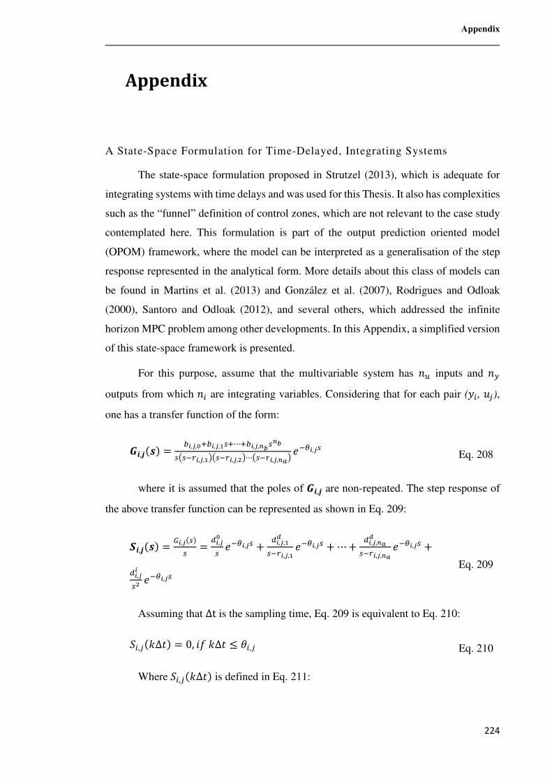
Appendix
224
Appendix
A State-Space Formulation for Time-Delayed, Integrating Systems
The state-space formulation proposed in Strutzel (2013), which is adequate for
integrating systems with time delays and was used for this Thesis. It also has complexities
such as the “funnel” definition of control zones, which are not relevant to the case study
contemplated here. This formulation is part of the output prediction oriented model
(OPOM) framework, where the model can be interpreted as a generalisation of the step
response represented in the analytical form. More details about this class of models can
be found in Martins et al. (2013) and González et al. (2007), Rodrigues and Odloak
(2000), Santoro and Odloak (2012), and several others, which addressed the infinite
horizon MPC problem among other developments. In this Appendix, a simplified version
of this state-space framework is presented.
For this purpose, assume that the multivariable system has MP inputs and MQ
outputs from which M' are integrating variables. Considering that for each pair (w', fÝ), one has a transfer function of the form:
/V,Õkim =Gx,�,t|Gx,�,��|⋯|Gx,�,#Ï�#Ï
�Ô�.Hx,�,�ÖÔ�.Hx,�,pÖ⋯Ô�.Hx,�,#QÖ ".Xx,�� Eq. 208
where it is assumed that the poles of /V,Õ are non-repeated. The step response of
the above transfer function can be represented as shown in Eq. 209:
_V,Õkim =²x,�k�m� = ,x,�t
� ".Xx,�� + ,x,�,��
�.Hx,�,� ".Xx,�� +⋯+ ,x,�,#Q��.Hx,�,#Q ".Xx,�� +
,x,�x
�p ".Xx,�� Eq. 209
Assuming that ∆t is the sampling time, Eq. 209 is equivalent to Eq. 210:
�',Ýk�∆¿m = 0, ¹+�∆¿ ≤ ç',Ý Eq. 210
Where �',Ýk�∆¿m is defined in Eq. 211:
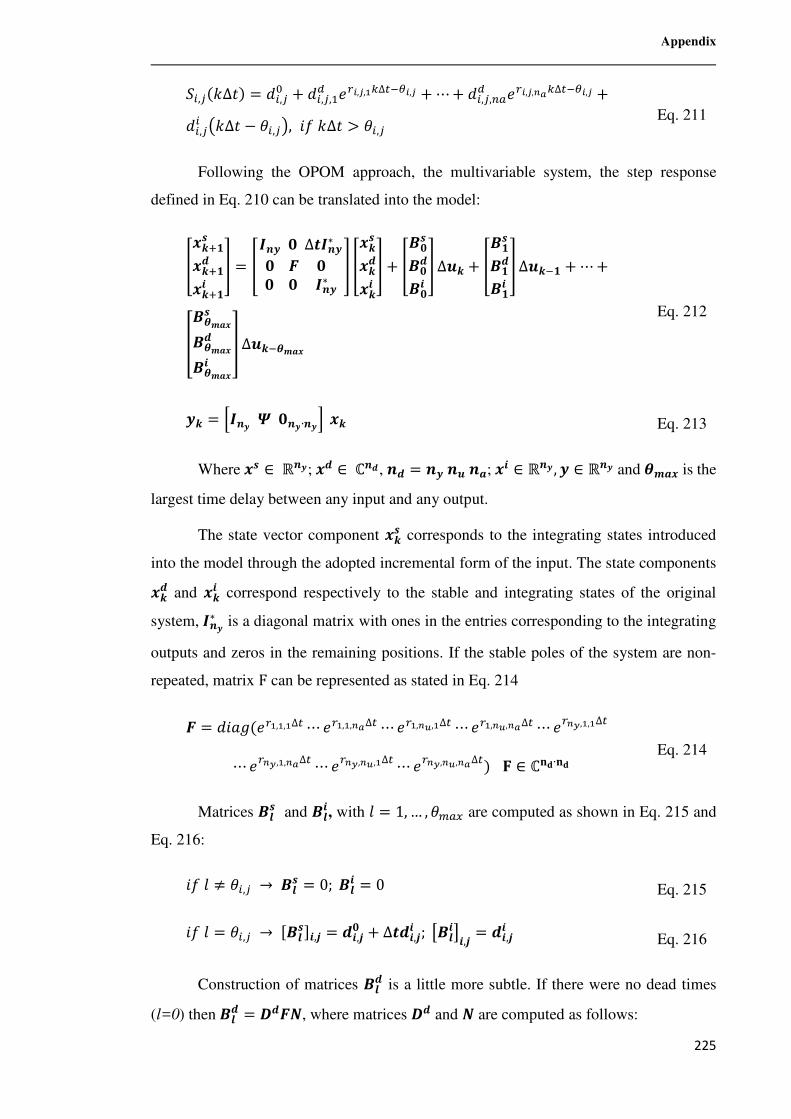
Appendix
225
�',Ýk�∆¿m = ë',ÝB + ë',Ý,�, "Hx,�,�(∆@.Xx,� +⋯+ ë',Ý,*?, "Hx,�,#Q(∆@.Xx,� +ë',Ý' Ô�∆¿ − ç',ÝÖ, ¹+�∆¿ > ç',Ý
Eq. 211
Following the OPOM approach, the multivariable system, the step response
defined in Eq. 210 can be translated into the model:
�\|�i
\|��
\|�V� = ��h�¾∆{�h�∗¾Ù¾
¾¾�h�∗� �\i\�\V
�+ ��¾i�¾��¾V
�∆�\ + ���i�����V
�∆�\.� +⋯+ �[��i
�[���
�[��V"∆�\.[��
Eq. 212
�\ = >�h� Ú¾h�∙h�C \ Eq. 213
Where i ∈ ℝh�;� ∈ ℂh� , h� = h�h�h�; V ∈ ℝh� , � ∈ ℝh� and [�� is the
largest time delay between any input and any output.
The state vector component \i corresponds to the integrating states introduced
into the model through the adopted incremental form of the input. The state components
\� and \V correspond respectively to the stable and integrating states of the original
system,�h�∗ is a diagonal matrix with ones in the entries corresponding to the integrating
outputs and zeros in the remaining positions. If the stable poles of the system are non-
repeated, matrix F can be represented as stated in Eq. 214
Ù = ë¹~Ak"H�,�,�∆@⋯ "H�,�,#Q∆@⋯ "H�,#�,�∆@⋯ "H�,#�,#Q∆@⋯ "H#�,�,�∆@ ⋯ "H#�,�,#Q∆@⋯ "H#�,#�,�∆@⋯ "H#�,#�,#Q∆@m Ý ∈ ℂ5Ð∙5Ð Eq. 214
Matrices ��i and ��V, with F = 1,… , ç�?� are computed as shown in Eq. 215 and
Eq. 216:
¹+F ≠ ç',Ý → ��i = 0;��V = 0 Eq. 215
¹+F = ç',Ý → µ��i·V,Õ = �V,Õ¾ + ∆{�V,ÕV ; &��V(V,Õ = �V,ÕV Eq. 216
Construction of matrices ��� is a little more subtle. If there were no dead times
(l=0) then��� = �Ù¡, where matrices � and ¡ are computed as follows:
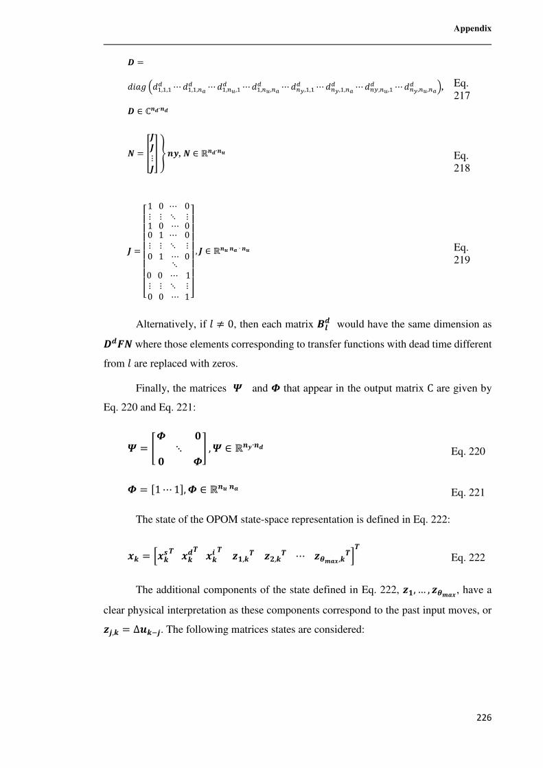
Appendix
226
=
ë¹~A ÷ë�,�,�, ⋯ ë�,�,*Q, ⋯ë�,*�,�, ⋯ë�,*�,*Q, ⋯ ë*�,�,�, ⋯ ë*�,�,*Q, ⋯ë*Q,*�,�, ⋯ë*�,*�,*Q, ø,
∈ ℂh�∙h�
Eq. 217
¡ = áá⋮á"Þh�, ¡ ∈ ℝh�∙h�
Eq. 218
á =
����������10⋯ 0⋮⋮⋱⋮10⋯ 001⋯ 0⋮⋮⋱⋮01⋯ 0⋱
00⋯ 1⋮⋮⋱⋮00⋯ 1 ��
��������, á ∈ ℝh�h�∙h� Eq.
219
Alternatively, if F ≠ 0, then each matrix ��� would have the same dimension as
�Ù¡ where those elements corresponding to transfer functions with dead time different
from F are replaced with zeros.
Finally, the matrices Ú and ß that appear in the output matrix C are given by
Eq. 220 and Eq. 221:
Ú = 7ß¾⋱¾ß: ,Ú ∈ ℝh�∙h� Eq. 220
ß = µ1⋯1·,ß ∈ ℝh�h� Eq. 221
The state of the OPOM state-space representation is defined in Eq. 222:
\ = >\ib\�b\V bã�,\bã ,\b ⋯ ã[��,\bCb Eq. 222
The additional components of the state defined in Eq. 222, ã�, … , ã[�� , have a
clear physical interpretation as these components correspond to the past input moves, or
ãÕ,\ = ∆�\.Õ. The following matrices states are considered:
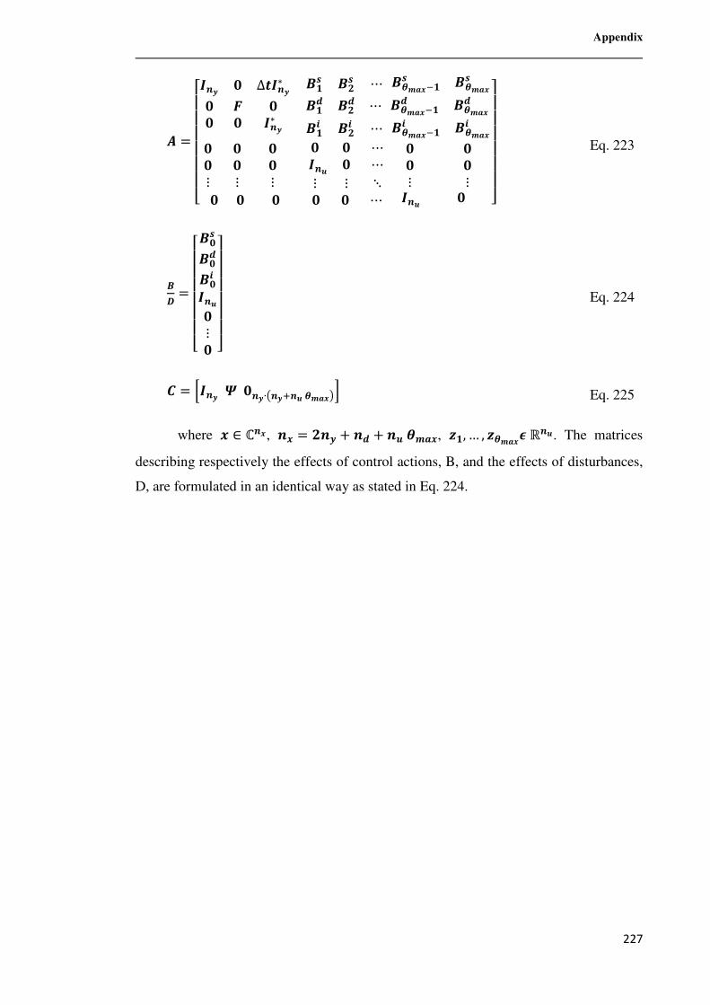
Appendix
227
� =
���������h� ¾ ∆{�h�∗¾ Ù ¾¾ ¾ �h�∗
��i � i ⋯ �[��.�i �[��i
��� � � ⋯ �[��.�� �[���
��V � V ⋯ �[��.�V �[��V
¾ ¾ ¾¾ ¾ ¾⋮ ⋮ ⋮
¾ ¾ ⋯�h� ¾ ⋯⋮ ⋮ ⋱
¾ ¾¾ ¾⋮ ⋮
¾ ¾ ¾¾ ¾ ⋯�h� ¾ �������� Eq. 223
� =
���������¾i�¾��¾V�h�¾⋮¾ ���
����� Eq. 224
� = >�h� Ú¾h�∙Ôh�|h�[��ÖC Eq. 225
where ∈ ℂh, h = h� + h� + h�[��, ã�, … , ã[��áℝh�. The matrices
describing respectively the effects of control actions, B, and the effects of disturbances,
D, are formulated in an identical way as stated in Eq. 224.
Appendix
228
Continuous-Time Transfer Functions for the Crude Oil Distillation Process
As discussed in the first part of this appendix, this work made use of the output
prediction oriented model (OPOM), a state-space formulation that is built upon the
transfer functions that define the interaction between each pair of
manipulated/disturbance and controlled variable. In order to identify these models, a
series of step tests were carried using the dynamic simulations of the four different
designs of the crude oil distillation process presented in Chapter 6. Table 35 to Table 58
display parameters to be substituted in Eq. 226 as a means to represent each model as a
5th order transfer function, which can be easily converted to any state-space formulation.
/V,Õk^m =Gx,�,t|Gx,�,��|Gx,�,p�p|Gx,�,s�s|Gx,�,r�r|Gx,�,¹�¹?x,�,t|?x,�,��|?x,�,p�p|?x,�,s�s|?x,�,r�r|?x,�,¹�¹ Eq. 226
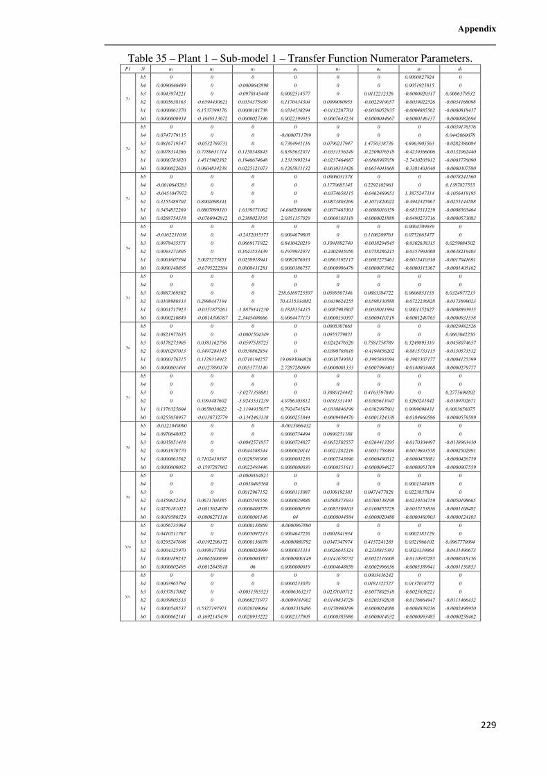
Appendix
229
Table 35 – Plant 1 – Sub-model 1 – Transfer Function Numerator Parameters. P1 N u1 u2 u3 u4 u5 u6 u7 d1
y1
b5 0 0 0 0 0 0 0.0000827924 0
b4 0.0090046489 0 -0.0000642898 0 0 0 0.0051925815 0
b3 0.0043974221 0 -0.0970145448 0.0002514577 0 0.0112212326 -0.0000020317 0.0006379532
b2 0.0005638163 -0.6594430621 0.0354375930 0.1170434304 0.0099090955 -0.0022919057 -0.0039022526 -0.0034168098
b1 0.0000061370 6.1537399176 0.0000181738 0.0314538294 -0.0112287701 -0.0056052935 -0.0004885562 -0.0000818437
b0 0.0000000934 -0.1649113672 0.0000027346 0.0022399915 -0.0007643234 -0.0000044667 -0.0000146137 -0.0000082694
y2
b5 0 0 0 0 0 0 0 -0.0039176576
b4 0.0747179135 0 0 -0.0000711789 0 0 0 0.0442060078
b3 0.0816719547 -0.0532769731 0 0.7364941116 0.0790217947 1.4750338736 4.6963905563 -0.0282380084
b2 0.0078314266 0.7789631714 0.1158548845 0.8395632971 -0.0331556249 -0.2509076518 -0.4239366006 -0.0132062440
b1 0.0000783820 1.4515902382 0.1946674648 1.2313993214 -0.0237464687 -0.6868907059 -2.7430205912 -0.0003776090
b0 0.0000022620 0.0604834238 0.0225121073 0.1265831132 -0.0010333426 -0.0654041668 -0.3381401040 -0.0000307580
y3
b5 0 0 0 0 0.0006031578 0 0 -0.0078241560
b4 -0.0010643203 0 0 0 0.1770685145 0.2292102963 0 0.1387827555
b3 -0.0451047972 0 0 0 -0.0374658115 -0.0462469651 1.3875247314 -0.1056419195
b2 0.3155489702 0.8002098341 0 0 -0.0873803269 -0.1071820022 -0.4942325967 -0.0255144588
b1 0.3454852269 0.6807099310 1.6339371062 14.6682006006 -0.0075465301 -0.0088016359 -0.6833511239 -0.0008565464
b0 0.0268754518 -0.0760942812 0.2388023195 2.0351357929 -0.0000103318 -0.0000021889 -0.0490273716 -0.0000573083
y4
b5 0 0 0 0 0 0 0.0004709939 0
b4 -0.0162231038 0 -0.2452035375 0.0004679805 0 0.1106209763 0.0752665477 0
b3 0.0978435571 0 0.0669171922 0.8430420219 0.3091892740 -0.0038294545 -0.0302638315 0.0259084502
b2 0.0093171805 0 0.1641553439 0.1979932971 -0.2402945056 -0.0758286215 -0.0357991060 -0.0638219403
b1 0.0001607394 5.0075273851 0.0258918941 0.0082076933 -0.0863192117 -0.0083275461 -0.0015410310 -0.0017041691
b0 0.0000148895 -0.6795222504 0.0008431281 0.0000186757 -0.0000986479 -0.0000073962 -0.0000315367 -0.0001405162
y5
b5 0 0 0 0 0 0 0 0
b4 0 0 0 0 0 0 0 0
b3 0.0867369582 0 0 258.6169725597 0.0589507346 0.0683384722 0.0606853155 0.0324977233
b2 0.0108980333 0.2998447194 0 70.4315334882 -0.0439624255 -0.0598330588 -0.0722236828 -0.0373699023
b1 0.0001717923 -0.0351875261 -1.8879141230 0.1818354435 -0.0087983807 -0.0038011994 0.0001152627 -0.0008893935
b0 0.0000210849 -0.0014306767 2.3445408666 0.0064477173 -0.0000150397 -0.0000410719 -0.0001240765 -0.0000931558
y6
b5 0 0 0 0 0.0005307665 0 0 -0.0029482526
b4 0.0821977635 0 -0.0001504349 0 0.0955779821 0 0 0.0663042250
b3 0.0178273905 0.0381162756 -0.0597518725 0 -0.0242476520 0.7581758789 0.3249895310 -0.0458074657
b2 0.0010297013 0.3497284145 0.0530862854 0 -0.0390703616 -0.4194856202 -0.0815733115 -0.0130573512
b1 0.0000176315 0.1129314912 0.0710194257 19.0693044826 -0.0018749581 -0.1995891094 -0.1903307177 -0.0004125399
b0 0.0000001491 -0.0127890170 0.0053773140 2.7287280009 -0.0000001333 -0.0007969403 -0.0140803468 -0.0000279777
y7
b5 0 0 0 0 0 0 0 0
b4 0 0 0 0 0 0 0 0
b3 0 0 -3.0271358881 0 0.3880124442 0.4163597840 0 0.2775690202
b2 0 0.1091487602 -5.9243531239 4.9786105812 0.0181331491 -0.0305611047 0.3260241842 -0.0109702671
b1 0.1376325604 0.0658030622 -2.1194935057 0.7924741674 -0.0330846199 -0.0362997601 0.0099098431 0.0003656075
b0 0.0255050957 -0.0138732779 -0.1342463138 0.0000251844 -0.0009484470 -0.0001324338 -0.0184660586 -0.0000559589
y8
b5 -0.0121949090 0 0 -0.0015066432 0 0 0 0
b4 0.0970648052 0 0 0.0000734494 0.0690251188 0 0 0
b3 0.0035051418 0 -0.0042571857 0.0000724827 -0.0652502557 -0.0264413295 -0.0170304497 -0.0138963430
b2 0.0001970770 0 0.0044588544 0.0000020141 -0.0021282216 -0.0051758494 -0.0019693558 -0.0002502991
b1 0.0000063562 0.7102439397 0.0029591906 0.0000003236 -0.0007543690 -0.0000490512 -0.0000455681 -0.0000426759
b0 0.0000000052 -0.1597287902 0.0022493446 0.0000000030 -0.0000351613 -0.0000094627 -0.0000051709 -0.0000007559
y9
b5 0 0 -0.0000164821 0 0 0 0 0
b4 0 0 -0.0010495568 0 0 0 0.0001548918 0
b3 0 0 0.0012967152 0.0000115087 0.0309192381 0.0471477828 0.0223837834 0
b2 0.0359652354 0.0671704385 0.0005591556 0.0000029886 -0.0508373933 -0.0700138198 -0.0239104759 -0.0050198665
b1 0.0276181022 -0.0015624070 0.0000409578 0.0000000539 -0.0085309103 -0.0100855729 -0.0035153836 -0.0001168482
b0 0.0019580329 -0.0006271116 0.0000001146 04 -0.0000044584 -0.0000020480 -0.0000460903 -0.0000124103
y10
b5 0.0056735964 0 0.0000138869 -0.0000967890 0 0 0 0
b4 0.0410511767 0 0.0005097213 0.0004647256 0.0001841934 0 0.0002185129 0
b3 0.0295247698 -0.0192206172 0.0000136878 -0.0000080792 0.0347347974 0.4157241285 0.0321966102 0.0967770094
b2 0.0004325970 0.0498177801 0.0000020999 0.0000031314 -0.0026645324 -0.2338815381 0.0024139064 -0.0431490673
b1 0.0000189232 -0.0062600699 0.0000000387 -0.0000000149 -0.0141678732 -0.0022116008 -0.0110937285 -0.0008018156
b0 0.0000002495 -0.0012845818 06 0.0000000019 -0.0004648858 -0.0002996656 -0.0005389941 -0.0001150853
y11
b5 0 0 0 0 0 0.0003436242 0 0
b4 0.0003965794 0 0 0.0000233070 0 0.0181322527 0.0137018772 0
b3 0.0337817002 0 -0.0051585523 -0.0006363237 0.0237010712 -0.0077802518 -0.0025838221 0
b2 0.0039805533 0 0.0060271977 -0.0009181902 -0.0149834729 -0.0203592838 -0.0176664947 -0.0111466432
b1 0.0000548537 0.5327197971 0.0020309064 -0.0003318486 -0.0170900199 -0.0000024080 -0.0004839236 -0.0002498950
b0 0.0000062141 -0.1692145439 0.0020933222 0.0002137905 -0.0000385986 -0.0000014032 -0.0000093485 -0.0000258462
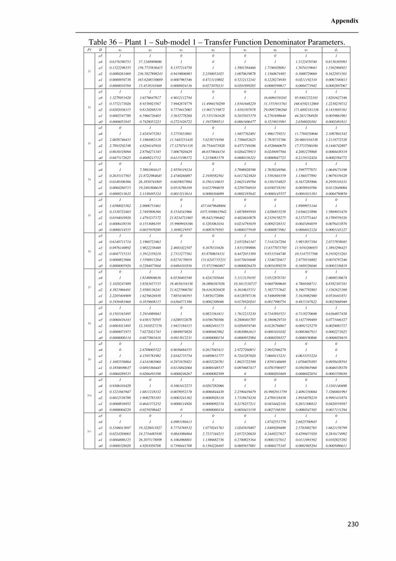
Appendix
230
Table 36 – Plant 1 – Sub-model 1 – Transfer Function Denominator Parameters. P1 D u1 u2 u3 u4 u5 u6 u7 d1
y1
a5 1 1 0 0 0 0 1 1
a4 0.6376390753 57.1240909686 1 0 1 1 1.5122470740 0.8136305093
a3 0.1322298355 156.7735836415 8.1357214750 1 1.5801584466 1.7196928081 1.5074339043 1.3362904921
a2 0.0080263469 236.5827898243 0.9439806983 2.2100051025 3.0070639878 1.3360674485 0.3008729069 0.1622953301
a1 0.0000950738 165.6208330689 0.0007965546 0.4713110802 0.5212112141 0.1228274930 0.0211192310 0.0067340413
a0 0.0000010704 15.4518103400 0.0000924136 0.0273070331 0.0201899285 0.0000599817 0.0004773942 0.0002897067
y2
a5 1 1 1 0 0 1 1 1
a4 1.3278953420 3.6576647817 4.9012112744 1 1 16.6094350165 95.8401252103 1.8201627346
a3 0.3752173026 8.9158923567 7.9942874779 11.4994150299 1.8341648229 31.1553933763 168.6592112869 1.2230239712
a2 0.0202036315 9.8120268519 9.7774412065 13.9017159872 1.4103307078 29.0997296260 171.6892181336 0.1433695161
a1 0.0002547788 6.5966726403 3.5632778260 15.5351561628 0.2035035379 6.2701698644 44.2651784920 0.0059863981
a0 0.0000051845 0.7428053223 0.2723426722 1.3937089513 0.0063406477 0.3219933993 2.6568020301 0.0002481811
y3
a5 0 1 1 0 1 1 1 1
a4 1 2.4245475283 5.2755653801 1 1.9457762481 1.9961759251 11.7769250694 2.1087801542
a3 2.0028746433 5.1984982118 11.5445251418 5.6238719390 1.7586052625 1.7818732706 20.9001916538 1.2119772528
a2 2.7893292198 4.8294145910 17.1270741318 30.7544473828 0.4571749186 0.4526660670 17.5715500180 0.1446742887
a1 0.8630318094 2.8794271345 7.0067920429 46.6570644154 0.0264278913 0.0249497504 4.2001278868 0.0060438319
a0 0.0475172625 0.4609213712 0.6115198372 5.2150081579 0.0000336321 0.0000047723 0.2119332424 0.0002584772
y4
a5 0 1 1 0 1 1 1 1
a4 1 7.5881091615 2.9559319124 1 3.7898928598 1.7658249566 1.5997777071 1.0649173198
a3 0.2635317565 21.8722984645 2.4740266887 2.1938582561 6.0117423820 1.5581603359 1.1360377891 1.9079339328
a2 0.0148306566 26.1850741805 0.6039037884 0.3563116655 2.6625149784 0.3301554825 0.1637285866 0.2958316331
a1 0.0004260715 19.2491806619 0.0516786169 0.0127994659 0.2295704910 0.0180718191 0.0058910766 0.0112649004
a0 0.0000213632 2.1338495124 0.0013213614 0.0000304089 0.0002185642 0.0000145557 0.0001031183 0.0004790850
y5
a5 1 1 0 1 0 0 1 0
a4 1.6580025362 2.0006753461 1 457.0479648004 1 1 1.8909971144 1
a3 0.3330722403 2.7495806366 8.1534543966 1075.9588635942 1.6878895950 1.6286853258 2.6566233896 1.5869053470
a2 0.0194010926 1.4793237172 21.8234721865 98.8421596462 0.4024010878 0.2329158275 0.2373771443 0.1789559326
a1 0.0006438550 0.1553686195 35.9909918166 0.3283061034 0.0234793039 0.0092526531 0.0045494059 0.0076433876
a0 0.0000314555 0.0035939288 3.3698219597 0.0087679585 0.0000375938 0.0000873961 0.0004012124 0.0003145127
y6
a5 1 1 0 0 1 1 1 1
a4 0.6140711714 2.1960723463 1 1 2.0352841347 7.5141247204 5.9853857184 2.0737858045
a3 0.0976140892 3.9822238468 2.4681022507 9.1676510426 1.8353589886 13.8377073705 11.9193206955 1.3893296425
a2 0.0047715333 3.3912359210 2.7313277561 83.8700654331 0.4472053389 9.8533544748 10.5147557568 0.1919253203
a1 0.0000823666 1.5590911264 0.8274170919 131.6245735233 0.0170416048 1.5246720417 2.9770516802 0.0074797246
a0 0.0000005926 0.2284077604 0.0484101856 15.9715960487 0.0000026470 0.0054389259 0.1609326046 0.0003336819
y7
a5 0 1 1 1 1 1 0 1
a4 1 1.8148804636 6.0536403540 6.4241505644 5.3113139195 5.0512876743 1 2.0608536674
a3 2.1020247489 3.8583457155 18.4650334338 36.0886567056 10.3013530737 9.6607909649 4.7869368711 6.8582307181
a2 4.3823966491 2.9580136241 21.6225906701 56.6163820428 6.3610635551 5.3827757642 9.3967792883 1.3362625300
a1 2.2205404909 1.6256626938 7.8854340393 5.8856372886 0.8128597136 0.5406899398 5.1618982900 0.0516441851
a0 0.1936483460 0.1839608115 0.6364571386 0.0002308046 0.0176920243 0.0017990754 0.4815347622 0.0025668940
y8
a5 1 1 0 1 1 1 1 1
a4 0.1503165495 5.2914989943 1 0.0823363411 1.7612233230 0.7143893521 0.7118270698 0.6364857458
a3 0.0060416343 9.4383170595 1.6288532678 0.0186780306 0.2808403785 0.1869629710 0.1427399489 0.0773446327
a2 0.0003013495 12.1910527159 1.9415184315 0.0002493173 0.0284959740 0.0126794867 0.0091525279 0.0029083717
a1 0.0000071973 7.0272021743 1.0849974820 0.0000465862 0.0030861613 0.0003410102 0.0003667913 0.0002271625
a0 0.0000000114 0.6875865416 0.0913812231 0.0000000154 0.0000952984 0.0000209327 0.0000190806 0.0000029419
y9
a5 0 1 1 1 1 1 0 0
a4 0 2.6709005522 0.9036684355 0.2617045411 2.9727260851 2.9932566279 1 0
a3 1 4.1595781982 2.0342735754 0.0489651777 6.7243287020 7.0669115231 4.0633355224 1
a2 1.1685556864 3.4141065060 0.2971676921 0.0032226781 1.8625722509 1.8595146699 1.0704070385 0.0958438593
a1 0.1850699637 0.6893360445 0.0116842004 0.0000348537 0.0859687417 0.0783596957 0.0565865968 0.0046538370
a0 0.0060289535 0.0266493390 0.0000246267 0.0000002589 0 0.0000201669 0.0006022054 0.0001558030
y10
a5 1 0 1 1 0 0 0 1
a4 0.9306103428 1 0.1063412273 0.0267282066 1 1 1 3.3101140498
a3 0.1221665947 1.6811218332 0.0078952170 0.0066844438 2.2590439479 16.9902911759 2.4091250004 7.3266801993
a2 0.0012536788 1.9082785185 0.0003241362 0.0000928110 1.7318674230 2.4789318458 1.8934078219 0.9991431874
a1 0.0000836952 0.4641571252 0.0000114926 0.0000092154 0.2176257211 0.0454442316 0.2651306812 0.0420559587
a0 0.0000004220 0.0259298442 0 0.0000000334 0.0050433158 0.0027168395 0.0080547305 0.0017131294
y11
a5 0 0 1 0 0 1 1 0
a4 1 1 4.0983180413 1 1 1.8742551779 2.6825700945 1
a3 0.3106013697 19.3228011827 8.7774769532 1.0770241763 3.0245839487 1.8409289498 2.5703082765 1.6621158799
a2 0.0224269003 24.2754485938 9.0843086864 2.7237344215 2.0572526620 0.2449227627 0.4299471920 0.2816174992
a1 0.0004886125 26.2075178899 6.1064968801 1.1386682736 0.2700825364 0.0001327012 0.0111093562 0.0102825282
a0 0.0000328028 4.9283050708 0.7390441708 0.1384226495 0.0005657081 0.0000175345 0.0001905284 0.0005086611
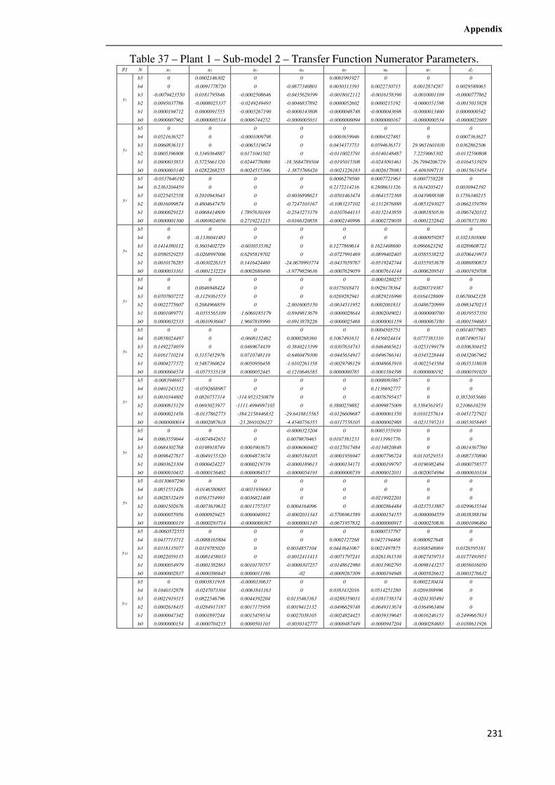
Appendix
231
Table 37 – Plant 1 – Sub-model 2 – Transfer Function Numerator Parameters. P1 N u1 u2 u3 u4 u5 u6 u7 d1
y1
b5 0 0.0002146302 0 0 0.0001991927 0 0 0
b4 0 -0.0091778720 0 -0.0877340801 0.0030313393 0.0022730715 0.0012874287 0.0029588065
b3 -0.0079423550 0.0181795846 -0.0002508646 -0.0435629399 -0.0018012112 -0.0016158390 -0.0010001109 -0.0000777862
b2 0.0095037786 -0.0008025337 -0.0249249493 -0.0046837892 0.0000052602 0.0000215192 -0.0000351598 -0.0015015828
b1 0.0000194712 0.0000091555 -0.0003267190 -0.0000143808 -0.0000048748 -0.0000043698 -0.0000013400 0.0000000542
b0 0.0000007962 -0.0000005514 0.0006744252 -0.0000005031 -0.0000000094 0.0000000167 -0.0000000534 -0.0000022689
y2
b5 0 0 0 0 0 0 0 0
b4 0.0521636527 0 -0.0001009798 0 0.0003659946 0.0004327485 0 0.0007363627
b3 0.0060836313 0 -0.0065319674 0 0.0434373753 0.0594636373 29.9651601030 0.0362862506
b2 0.0005396908 0.3349364887 0.0171041502 0 -0.0110023791 -0.0140148487 7.2259065302 -0.0132590808
b1 0.0000033853 0.5725661320 0.0244778080 -18.5684789504 -0.0195015508 -0.0243091461 -26.7994206729 -0.0164533929
b0 0.0000003148 0.0282268255 0.0024515306 -1.3873768420 -0.0021226183 -0.0026178983 -4.4093097111 -0.0015633454
y3
b5 -0.0337646192 0 0 0 0.0006279500 0.0007721963 0.0007758228 0
b4 0.2363204459 0 0 0 0.2172214216 0.2808631326 0.1634205421 0.0030942392
b3 0.0225452558 0.2010943643 0 -0.0036898623 -0.0501463474 -0.0641572368 -0.0439888308 0.1756340215
b2 0.0016099874 0.4804647470 0 -0.7247103167 -0.1083237102 -0.1312876888 -0.0853293027 -0.0662359789
b1 0.0000029123 0.0068414809 1.7897630169 -0.2543273379 -0.0107644133 -0.0132143858 -0.0081850536 -0.0967420312
b0 0.0000001300 -0.0069024056 0.2719221215 -0.0166320858 -0.0002140996 -0.0002729038 -0.0001252842 -0.0078371380
y4
b5 0 0 0 0 0 0 0 0
b4 0 -0.1336041481 0 0 0 0 -0.0000959287 0.1023303000
b3 0.1414380112 0.3603402729 -0.6030535362 0 0.1277869614 0.1623408600 0.0966623292 -0.0289608721
b2 0.0580529255 -0.0268997006 0.6295819702 0 -0.0727991469 -0.0899402405 -0.0585538252 -0.0706419973
b1 0.0010176285 -0.0030226315 0.1416424460 -24.0670993774 -0.0437659767 -0.0519242744 -0.0355953678 -0.0086890873
b0 0.0000033161 -0.0001232224 0.0002680490 -3.9779829636 -0.0007629059 -0.0007614144 -0.0006209541 -0.0001929708
y5
b5 0 0 0 0 0 -0.0003280257 0 0
b4 0 0.0046948424 0 0 0.0375018471 0.0929178364 0.0280719387 0
b3 0.0707807272 -0.1129361573 0 0 0.0269282941 -0.0829216990 0.0164128009 0.0670042328
b2 0.0022775607 0.2684966859 0 -2.0016005150 -0.0634511952 0.0002001833 -0.0486720999 -0.0983470215
b1 0.0001089771 -0.0355565109 -1.6060185179 -0.8949813679 -0.0000028644 -0.0002049021 -0.0000000700 -0.0039557350
b0 0.0000032533 -0.0010936047 1.9607818990 -0.0913878226 -0.0000025468 -0.0000001159 -0.0000067180 -0.0001594683
y6
b5 0 0 0 0 0 0.0004505751 0 0.0014077985
b4 0.0858024497 0 -0.0608132462 0.0000268360 0.1067491631 0.1456024414 0.0777383310 0.0874905741
b3 0.1492274059 0 0.0469674439 -0.3840213399 -0.0307634743 -0.0464665621 -0.0253199179 -0.0306304452
b2 0.0161710214 0.3157452976 0.0710748110 -0.6460479300 -0.0445654917 -0.0496766341 -0.0345228444 -0.0432067962
b1 0.0004277372 0.5487360624 0.0050956458 -1.0102261358 -0.0029798129 -0.0048663910 -0.0022543584 -0.0035318038
b0 0.0000004574 -0.0575535158 0.0000052445 -0.1210646585 0.0000000785 -0.0001584398 0.0000000192 -0.0000391020
y7
b5 -0.0083946917 0 0 0 0 0.0008093867 0 0
b4 0.0401243332 -0.0592688987 0 0 0 0.1136692777 0 0
b3 0.0010344802 0.0820757314 -314.9523250879 0 0 -0.0076795437 0 0.3852055680
b2 0.0000815129 0.0693023977 -1111.4994997105 0 0.3800259882 -0.0099875009 0.3384561951 0.2106610259
b1 0.0000021456 -0.0137862773 -384.2158446832 -29.6418815565 -0.0126609687 -0.0000001350 0.0101257614 -0.0451727921
b0 -0.0000000014 -0.0002087618 -23.2691026127 -4.4540756355 -0.0317558105 -0.0000002988 -0.0231595213 -0.0053058495
y8
b5 0 0 0 -0.0000323204 0 0.0005355930 0 0
b4 0.0063559044 -0.0074842651 0 0.0079870465 0.0107381233 0.0113991776 0 0
b3 0.0684302768 0.0198918749 0.0003903671 -0.0006060402 -0.0127017484 -0.0134820848 0 -0.0014367760
b2 0.0098427817 -0.0049155320 0.0004873674 -0.0005184105 -0.0001956947 -0.0007796724 0.0110529353 -0.0087370890
b1 0.0003623304 0.0000424227 0.0000219739 -0.0000189613 -0.0000134171 -0.0000199797 -0.0196982484 -0.0000758577
b0 0.0000010432 -0.0000156402 0.0000084517 -0.0000054193 -0.0000000739 -0.0000012031 -0.0020074994 -0.0000010334
y9
b5 -0.0130697290 0 0 0 0 0 0 0
b4 0.0851551426 -0.0146580685 -0.0031936663 0 0 0 0 0
b3 0.0028532439 0.0563754993 0.0036821408 0 0 -0.0219922201 0 0
b2 0.0001502676 -0.0073639632 0.0011757357 0.0004164096 0 -0.0002864484 -0.0237533887 -0.0299635544
b1 0.0000055956 0.0000929425 0.0000040912 -0.0002031343 -0.5706961589 -0.0000154155 -0.0000004559 -0.0038388194
b0 0.0000000119 -0.0000293714 -0.0000000367 -0.0000001145 -0.0671957832 -0.0000000917 -0.0000250836 -0.0001096460
y10
b5 -0.0060572555 0 0 0 0 0.0000737797 0 0
b4 0.0437713712 -0.0088165804 0 0 0.0002127268 0.0427194468 0.0000927648 0
b3 0.0318135077 0.0319785020 0 0.0034857104 0.0443641067 0.0021497875 0.0368548069 0.0326595181
b2 0.0022059135 -0.0081458033 0 -0.0012411413 -0.0071797241 -0.0261361530 -0.0027459713 -0.0177493951
b1 0.0000054979 -0.0001382865 0.0010170757 -0.0000307257 -0.0148612980 -0.0013902795 -0.0098143257 -0.0056016050
b0 0.0000002837 -0.0000386645 0.0000013186 -02 -0.0009267309 -0.0000194948 -0.0005826612 -0.0003276632
y11
b5 0 0.0003831918 -0.0000330637 0 0 0 0.0002230434 0
b4 0.1040332878 -0.0247073304 -0.0061841163 0 0.0383432016 0.0514251280 0.0269388996 0
b3 0.0021919315 0.0822546796 0.0044392204 0.0135463363 -0.0288359031 -0.0381738374 -0.0201305491 0
b2 0.0002618435 -0.0284917187 0.0017175958 0.0019412132 -0.0496629748 -0.0649313674 -0.0364963404 0
b1 0.0000047342 0.0001897244 0.0015459534 0.0027038105 -0.0024824425 -0.0039339645 -0.0016246151 -0.2499667813
b0 0.0000000154 -0.0000704215 0.0000501103 -0.0030142777 -0.0000487449 -0.0000947204 -0.0000284683 -0.0188611926
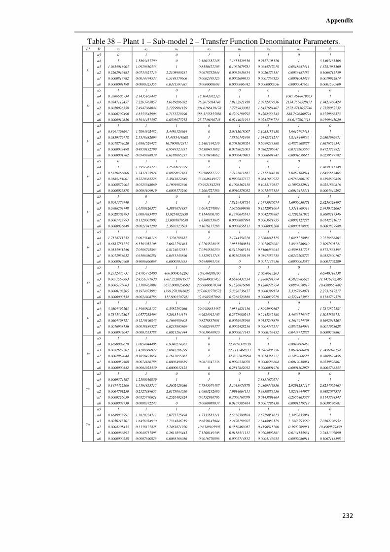
Appendix
232
Table 38 – Plant 1 – Sub-model 2 – Transfer Function Denominator Parameters. P1 D u1 u2 u3 u4 u5 u6 u7 d1
y1
a5 0 1 0 1 1 1 0 1
a4 1 1.5863431790 0 2.1803382245 1.1653529350 0.9127108126 1 3.1465133506
a3 1.9634013903 1.0929610333 1 0.8550422205 0.1062679781 0.0644747018 0.0818647411 1.3281985360
a2 0.2262916483 0.0733621716 2.2108900231 0.0678752044 0.0032936354 0.0026376131 0.0053487386 0.1066712159
a1 0.0000817782 0.0014374533 0.5148179606 0.0002395325 0.0002699555 0.0001767125 0.0001043429 0.0019922814
a0 0.0000094198 0.0000325355 0.0331597387 0.0000068608 0.0000006742 0.0000000556 0.0000047653 0.0001530909
y2
a5 1 1 0 1 0 0 1 0
a4 0.3586605734 3.1435165448 1 18.1643362325 1 1 1087.4648679863 1
a3 0.0347112457 7.2263765857 1.6189296032 76.2075014748 1.9132921918 2.0312439336 2154.7558528451 1.9421480424
a2 0.0020026558 7.4947368044 2.1229981129 304.6166419178 1.7759833082 1.8457684467 2572.4713057740 1.7558052732
a1 0.0000207490 4.8353542906 0.7153229996 388.3135855956 0.4209199792 0.4262556543 888.7696869794 0.3759866373
a0 0.0000010856 0.5641451307 0.0503075212 25.7746010743 0.0244031913 0.0243706714 64.0157601313 0.0199645020
y3
a5 1 1 1 0 1 1 1 0
a4 0.3991593691 1.7094392482 5.4486123664 0 2.0415018007 2.1085185438 1.9612797413 1
a3 0.0339379718 2.5318482096 11.4383418668 1 1.8850142499 1.9142321211 1.8118449836 2.0303986971
a2 0.0018764020 1.6801529425 16.7909812311 2.2401194239 0.5085058024 0.5099233388 0.4876968877 1.8676529341
a1 0.0000033498 0.4850132799 6.9549123331 0.6389431682 0.0358021003 0.0362296041 0.0329505560 0.4723729921
a0 0.0000001762 0.0349938839 0.6188665237 0.0378474662 0.0006410903 0.0006694947 0.0004659655 0.0259577782
y4
a5 0 1 1 0 0 0 0 1
a4 1 1.2951765223 3.2520621379 1 1 1 1 1.9659315548
a3 0.5326458606 1.2432125924 6.8929852163 6.0586652722 1.7125811687 1.7512344638 1.6462184814 1.6455653465
a2 0.0585181001 0.2220385226 2.3841822849 33.0046149577 0.9902837377 0.9841650722 0.9763860107 0.3594607856
a1 0.0008872903 0.0125548069 0.1901982596 50.9921842281 0.1098362138 0.1053159357 0.1097852944 0.0251860816
a0 0.0000025378 0.0003109919 0.0003575290 5.2604727386 0.0016378032 0.0013455154 0.0016415341 0.0004649292
y5
a5 1 0 0 0 1 1 1 1
a4 0.7041379740 1 1 1 1.8129458714 1.6775030674 1.6906030371 2.3236528497
a3 0.0986204748 1.6580126375 4.3884671837 3.6041274084 1.6356099496 0.1512081004 1.5311969514 2.9430452663
a2 0.0028502793 1.0604933480 15.9254022438 8.1144306105 0.1370645541 0.0042303887 0.1292581932 0.3608217346
a1 0.0001423993 0.1120001902 25.0038678638 1.8388353645 0.0000687994 0.0003671955 0.0002127275 0.0142521013
a0 0.0000026649 0.0021941299 2.3630123503 0.1076137288 0.0000056511 0.0000002200 0.0000178802 0.0003829989
y6
a5 1 1 1 0 1 1 1 1
a4 1.7514711252 3.0623146116 2.3226288187 1 2.1744554220 2.3064448515 2.0455218086 2.2278636863
a3 0.6583751275 6.5563052108 2.6612791463 4.2763828835 1.9851500854 2.0078676081 1.8833286610 2.1097605721
a2 0.0555031246 7.0386792863 0.8124032351 7.0193830250 0.5122965154 0.5166456043 0.4898531725 0.5731863595
a1 0.0012953632 4.6306050281 0.0453345896 6.5329211718 0.0256250119 0.0397586735 0.0242208776 0.0352600767
a0 0.0000010900 0.9606460068 0.0000503355 0.6940991158 0 0.0011135936 0.0000003587 0.0003702289
y7
a5 1 1 1 1 0 1 0 1
a4 0.2512475731 2.4705772400 406.0004562291 10.8584288100 1 2.0690613263 1 4.6940318138
a3 0.0071567393 2.4556371630 1961.7520011917 60.8840037455 4.6546437534 1.2860244374 4.5820985625 11.1476292586
a2 0.0005175063 1.5189765894 3677.0068254992 239.6080670394 9.1526816090 0.1280276754 9.0889078817 10.4580667082
a1 0.0000103205 0.1974073983 1399.2763018625 337.6633778572 5.3326736457 0.0000399174 5.3367394071 2.2731617217
a0 0.0000000134 0.0024908786 111.8001507921 32.6985057066 0.5266523888 0.0000039719 0.5224473956 0.1144739578
y8
a5 1 1 1 1 1 1 0 1
a4 3.0504392263 1.3903808122 0.5582292966 29.0988633487 1.9834821136 1.8095909167 1 1.7812822383
a3 0.7315342305 1.0577258493 1.2018544174 6.9624012105 0.2571980245 0.2945232188 3.4656779367 1.5055856751
a2 0.0604398121 0.1210196845 0.1666989405 0.8278837601 0.0056938940 0.0137248879 4.3616914398 0.1692941205
a1 0.0016968156 0.0038189527 0.0233805869 0.0682349377 0.0002428236 0.0004345511 0.8835584044 0.0013953628
a0 0.0000032047 0.0003553788 0.0021261344 0.0039630920 0.0000013145 0.0000163452 0.0438712875 0.0000203861
y9
a5 1 1 1 0 1 0 1 0
a4 0.1690003618 1.0654944405 0.9340274267 0 12.4756378719 1 0.8049609463 1
a3 0.0052687202 1.4208060977 2.0942286299 0 22.1117468233 0.0905405756 1.8674606401 1.7456078154
a2 0.0002969044 0.1658473654 0.1612055062 1 32.4322828994 0.0014365377 0.1482006585 0.3868629456
a1 0.0000059368 0.0074166788 0.0003490659 0.0813347336 6.9020534078 0.0000583804 0.0019038054 0.0239826861
a0 0.0000000342 0.0004923439 0.0000032125 0 0.2817842012 0.0000001976 0.0001502978 0.0004738553
y10
a5 1 1 0 0 0 1 0 0
a4 0.9069574187 1.2500616859 1 1 1 2.8851670571 1 1
a3 0.1474422506 1.5191853715 0.3602428086 5.7345674487 3.1613973878 2.4869349356 2.9291231117 2.8254065465
a2 0.0064791250 0.2527339655 2.0173064550 1.0883232686 1.9914664151 0.3858883536 1.8231944977 0.9882077373
a1 0.0000226059 0.0125770621 0.2526402824 0.0152910706 0.3000167079 0.0143891464 0.2656463577 0.1143734343
a0 0.0000009730 0.0008372243 0 0.0000988037 0.0107585464 0.0001795438 0.0091519719 0.0039596981
y11
a5 1 1 1 1 1 1 1 0
a4 0.1689933991 1.3620224712 2.0773725498 4.7333583211 2.5330580504 2.6729051613 2.3452855084 1
a3 0.0056213301 1.6458034930 2.7334846259 9.6850145044 2.2498199207 2.3448082179 2.1443793560 7.0162296952
a2 0.0004205433 0.3138127425 1.7461871920 10.6349105993 0.3850463087 0.4196815266 0.3602769951 10.4909879450
a1 0.0000066893 0.0040711895 0.2611855443 7.1200149308 0.0158511132 0.0204092881 0.0134133634 2.2441307690
a0 0.0000000258 0.0007690826 0.0068166056 0.9016776896 0.0002714832 0.0004146653 0.0002086911 0.1067113398
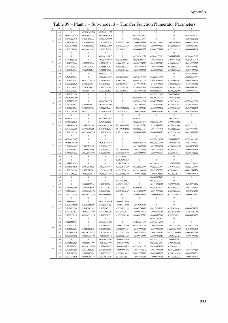
Appendix
233
Table 39 – Plant 1 – Sub-model 3 – Transfer Function Numerator Parameters. P1 N u1 u2 u3 u4 u5 u6 u7 d1
y1
b5 0 -0.0000304206 -0.0004811173 0 0 0 0 0
b4 -0.0967598548 -0.0009884211 -0.0296067046 0 0.0024055083 0 0 0.0038449213
b3 0.0757443938 0.0018699441 -0.0025507392 0 0.0012435071 0 0 -0.0018803664
b2 0.0402694524 0.0037816404 0.0005873454 0.1872027740 -0.0004363791 0.0064371603 0.0014603898 -0.0007214263
b1 0.0008788880 0.0011459035 -0.0000212824 0.3804417343 -0.0020497651 -0.0003911489 -0.0016085650 -0.0000010313
b0 0.0000024289 -0.0000059921 0.0000070799 0.0611929572 -0.0000691372 -0.0041725982 -0.0000012559 -0.0000003004
y2
b5 0 0 0 0 0 0 0 0
b4 0 0 -0.0004595011 0 0.0009349578 0.0964977502 0.0004338471 0.0010607255
b3 0.1701853788 0 -0.0154080337 0.2929186916 0.1098390664 -0.0330707891 0.0436993928 0.0543642719
b2 0.0645609446 0.0785754810 0.0209652632 0.3446787536 -0.0402159523 -0.0325872920 -0.0149114427 -0.0195216732
b1 0.0000126727 0.1500729702 0.0288375261 0.5291807252 -0.0424606605 -0.0026768588 -0.0218512442 -0.0247581780
b0 0.0000240915 0.0095622703 0.0021209980 0.0649327586 -0.0034825132 -0.0000007496 -0.0021296606 -0.0021241143
y3
b5 0 0 -0.0034423830 0 0 0 0 0.0028266091
b4 0.2933262611 0 -0.2178252255 0.0012458682 0.0032479772 0.3126539383 0 0.2206005931
b3 0.0037663145 -0.0073530113 0.1401979813 0.4167266571 0.3968248155 -0.0979865917 3.2373336680 -0.0953843127
b2 0.0006276029 0.1388094874 0.1968575734 0.0859389794 -0.1491127943 -0.1453533498 -1.6801852762 -0.1096309346
b1 0.0000084007 0.2324094432 0.0170033709 0.0002299544 -0.1860377963 -0.0105997862 -1.4104925956 -0.0076602082
b0 0.0000000291 -0.0356017729 0.0000143683 0.0000466836 -0.0132415865 0.0000001275 -0.0882192990 -0.0000777037
y4
b5 0.0056303574 0 0 0 0 0.0017757943 0.0010649518 0
b4 -0.5768002099 0 0 0 0.0018503252 0.1356180743 0.0786049685 0
b3 0.9627108377 0 -0.0047701229 0 0.1804136720 -0.0081378350 -0.0136045652 0.8790667934
b2 0.1807511817 0.0851166922 -0.3508763309 0 -0.0339960560 -0.1089559456 -0.0710357052 -0.1041722242
b1 0.0067432843 0.1696093864 0.0644862404 35.0254446464 -0.1419415046 -0.0094952184 -0.0059001702 -0.8932084302
b0 0.0000094498 -0.0347332831 0.1771092640 7.4652959797 -0.0061583284 -0.0002858034 -0.0001489775 -0.0255336445
y5
b5 0 0 0 0 0 0 0 0
b4 -0.0997037821 0 -0.4500685627 0 0.0902973172 0 0.0412096157 0
b3 0.1459416038 0 0.4059725295 0 0.0191763759 0.1771056001 0.0123993562 0
b2 0.0334931150 0.0530276560 -0.0046429290 35.2806476778 -0.1161101580 -0.1920668770 -0.0584595608 0.2172711511
b1 0.0000392396 0.1334069169 0.0047835183 16.4295202161 0.0000021175 -0.0111699596 -0.0062537222 -0.2777015389
b0 0.0000025036 -0.0324804720 0.0000139824 0.1260652020 -0.0000014995 -0.0007044555 -0.0003545904 -0.0220038195
y6
b5 0 0 0 0 0 0 0 0
b4 -0.0004675831 0 0 0 0 0.0007157070 0.0004893828 0.0823001165
b3 -0.0666103798 0 -0.2676786259 0 0.1618401644 0.1228331290 0.0708239799 -0.0313958109
b2 0.2087545187 0.0472180377 0.1795643659 0 -0.0598624839 -0.0378395231 -0.0244844278 -0.0400162512
b1 0.2074568881 0.0881291009 0.2066113331 17.2795835259 -0.0652118665 -0.0511321408 -0.0335057212 -0.0046856523
b0 0.0131703726 -0.0118095499 0.0001926803 2.0582675939 -0.0040324235 -0.0033729533 -0.0022635411 -0.0001764549
y7
b5 0 0 0 0.0003960432 0 0 0 0
b4 0 0 0 0.0636796773 0 0 0 0
b3 0.0741208265 0 0 0.0173826029 0 0.5394954237 0.3635085128 0.4112716783
b2 0.0328476819 0.0172579835 -2.6721977459 0.0002649429 0.7420823303 0.0107212801 0.0530503394 0.1673423923
b1 0.0000045688 0.0216876943 -2.5838894295 0.0000227459 0.0001344630 -0.0739762568 -0.0364941213 -0.0623591554
b0 0.0000089132 -0.0052030159 -0.2055267629 0.0000000139 -0.0794124225 -0.0029112182 -0.0013249714 -0.0023645576
y8
b5 0 0 0 0 0 -0.0063925466 0 0
b4 0 0 0 0.0001026033 0 0.4701152233 0 0
b3 0 0.0049959836 0.0018195983 0.0000332704 0 -0.5212368032 0.0241700324 -0.0230110074
b2 0.2411165069 0.0117398640 0.0000092617 0.0000004157 0.0866805382 0.0001641637 -0.0408932188 -0.0135836427
b1 0.0287416034 -0.0056688548 0.0000061724 0.0000001260 -0.1258846718 -0.0012919484 -0.0000201526 -0.0003656413
b0 0.0000004719 -0.0000551889 -0.0000000061 03 -0.0000749529 -0.0000014223 -0.0000010659 -0.0000170570
y9
b5 0 0 0 0 0 0 0 0
b4 0.0497344087 0 -0.0033056454 -0.0000125879 0 0 0 0
b3 0.0058706050 0.0020056980 0.0023038402 -0.0006560784 -0.0198088948 0 0 0
b2 0.0001555260 0.0040816319 0.0023817555 0.0001722519 -0.0041790486 -0.0278235870 -0.0164384305 -0.0686159728
b1 0.0000124831 -0.0002274497 0.0007858726 0.0000132644 -0.0000527292 -0.0022620946 -0.0014284604 -0.1063029955
b0 0.0000000658 -0.0000713210 0.0000351091 0.0000174236 -0.0000102258 -0.0000017045 -0.0000002121 -0.0086614055
y10
b5 0 0 0 0 0 0.0002468965 0 0
b4 0.0497222865 0 -0.0018456209 0 0.0771085143 0.0530115805 0 0
b3 0.1624272265 0 0.0018350115 -0.0061221821 0.0007292580 -0.0056877641 12.9621447071 0.0360322429
b2 0.0011747171 0.0420119747 0.0006960273 0.0017809492 -0.0327787949 -0.0252289037 20.1871287867 -0.0204498601
b1 0.0001387676 -0.0186320257 0.0004168678 0.0000613299 -0.0013168704 -0.0012354086 -14.3512831331 -0.0039670023
b0 0.0000007692 -0.0006685108 -0.0000000615 0.0000001408 -0.0000100117 -0.0000008527 -1.1353433423 -0.0001378550
y11
b5 0 0 -0.0000934202 -0.0000183621 0 0.0005417753 0.0003286385 0
b4 0.1365172836 -0.0000661001 -0.0046557073 -0.0018390046 0 0.0447057305 0.0237660745 0
b3 0.0262371205 -0.0026124443 0.0034097977 -0.0000195326 0.0680361355 -0.0388019267 -0.0210196327 0
b2 0.0014844508 0.0090516703 0.0023949468 -0.0000981210 -0.0643536292 -0.0657235635 -0.0372750394 -0.0262663223
b1 0.0000175874 0.0063418806 0.0010802997 0.0001812689 -0.0837513303 -0.0024093602 -0.0016661070 -0.0405761206
b0 0.0000009636 -0.0066301879 0.0003404349 0.0000072024 -0.0044569281 -0.0000115763 -0.0000292552 -0.0021460877
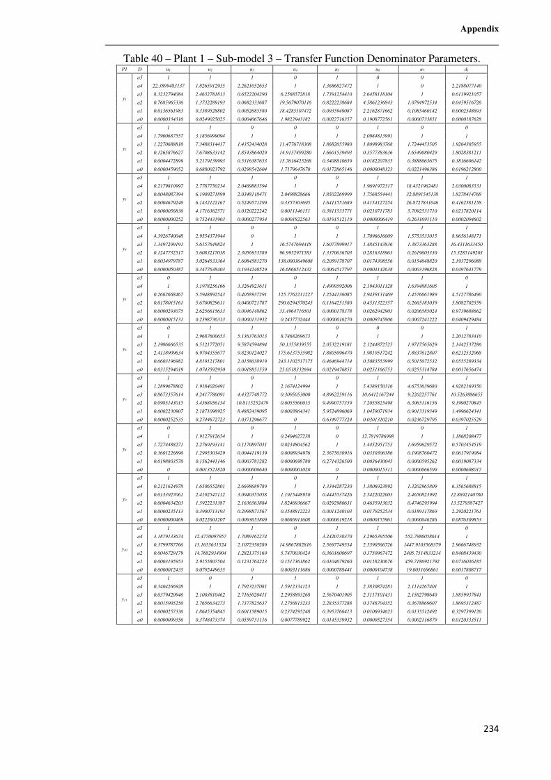
Appendix
234
Table 40 – Plant 1 – Sub-model 3 – Transfer Function Denominator Parameters. P1 D u1 u2 u3 u4 u5 u6 u7 d1
y1
a5 1 1 1 0 1 0 0 1
a4 22.3899483137 1.8265912935 2.2621052653 1 1.3686827472 1 0 2.2188077140
a3 8.3232794084 2.4632781813 0.6522204290 6.2568572818 1.7391254410 2.6458118104 1 0.6119921057
a2 0.7685965336 1.3732289193 0.0682333687 19.5679070116 0.8222238684 4.5861236843 1.0794972534 0.0459516726
a1 0.0136561983 0.3389528802 0.0052685580 18.4285107472 0.0935949087 2.2162871662 0.1085460142 0.0002548693
a0 0.0000334310 0.0249025025 0.0004067646 1.9822943182 0.0022716357 0.1908772561 0.0000733851 0.0000187628
y2
a5 1 1 0 0 0 1 0 0
a4 1.7900687557 3.1856999094 1 1 1 2.0984813991 1 1
a3 1.2270688810 7.3488314417 1.4352434028 11.4776718308 1.8682055980 1.8098983768 1.7244453505 1.9264305955
a2 0.1265876627 7.6708633142 1.8543864029 14.9137499280 1.6601539493 0.3577383636 1.6549080429 1.8028381211
a1 0.0004472899 5.2179139993 0.5316387653 15.7616425268 0.3408810659 0.0182207835 0.3888063675 0.3816696142
a0 0.0000459052 0.6880023792 0.0298542604 1.7179647670 0.0172865146 0.0000048123 0.0221496386 0.0196212800
y3
a5 1 1 1 0 0 1 1 1
a4 0.2179810997 2.7787750234 2.0469883594 1 1 1.9691972317 18.4321962481 2.0300083531
a3 0.0048087394 6.1909271899 2.0348118471 2.0498828666 1.8502269999 1.7568554441 32.8891545138 1.8278414768
a2 0.0004679240 6.1432122167 0.5249571299 0.3357303695 1.6411551689 0.4154127254 26.8727831046 0.4162581158
a1 0.0000056830 4.1716362571 0.0320222242 0.0011146151 0.3811533771 0.0210711783 5.7092531710 0.0217820114
a0 0.0000000252 0.7524431903 0.0000277954 0.0001822563 0.0191512119 0.0000006419 0.2631691110 0.0002094602
y4
a5 1 1 0 0 0 1 1 1
a4 4.3926740048 2.9554371944 0 1 1 1.7096616009 1.5753533015 8.9656148171
a3 1.3497299191 5.6157649824 1 16.5747694418 1.6077899917 1.4845143836 1.3873363288 16.4311633450
a2 0.1247732517 5.6083217038 2.3056953589 96.9952971583 1.3370636703 0.2816318963 0.2619603330 15.3285149203
a1 0.0034979787 3.0264533364 1.6084581270 138.0003649608 0.2059178707 0.0174308556 0.0154048820 2.1937296088
a0 0.0000050387 0.3477638403 0.1934240529 16.6866512432 0.0064517797 0.0004142638 0.0003196828 0.0497641779
y5
a5 0 1 1 0 1 1 1 0
a4 1 3.1978256166 3.3264923611 1 1.4909592006 2.1943011128 1.6394881605 1
a3 0.2662668467 5.5948892543 0.4058937291 125.7762211227 1.2544136085 2.9439131469 1.4576661989 4.5127786490
a2 0.0178015161 5.6700829611 0.0400721787 290.6294570245 0.1164251580 0.4531322357 0.2665183039 5.8082702559
a1 0.0000293075 2.6256615633 0.0046148862 33.4964716501 0.0000178378 0.0262942903 0.0206585024 0.9739688662
a0 0.0000015131 0.2398736313 0.0000131932 0.2437732444 0.0000016270 0.0009745806 0.0007241222 0.0409429484
y6
a5 0 1 1 1 0 0 0 1
a4 1 2.9687600653 5.1363763013 8.7468269673 1 1 1 2.2012783410
a3 2.1986666535 6.5121772051 9.5874594894 50.1355839555 2.0532219181 2.1244872525 1.9717565629 2.1442537286
a2 2.4118909634 6.9704355677 9.8230124027 175.6137535982 1.8805096470 1.9819517242 1.8837612807 0.6212532068
a1 0.6603196982 4.8191217801 2.0158038919 243.1102517175 0.4646944714 0.5083553999 0.5015072532 0.0555289334
a0 0.0315294019 1.0743592950 0.0018851559 25.0518332694 0.0219476851 0.0251166753 0.0255314784 0.0017656474
y7
a5 1 1 0 1 0 1 1 1
a4 1.2899678802 1.9184020491 1 2.1674124994 1 5.4389150316 4.6753639680 4.9282169350
a3 0.8673357614 4.2417780091 4.4327748772 0.3095053000 4.8962259116 10.6412167244 9.2202257761 10.5263886655
a2 0.0985143015 3.4368956134 10.8115252479 0.0055560015 9.4990757359 7.2055825498 6.3065116156 9.1990270845
a1 0.0002230907 2.1871098925 8.4882439095 0.0003864341 5.9524896069 1.0459071934 0.9013319349 1.4996624341
a0 0.0000252535 0.2744672723 1.0371296677 0 0.6349777324 0.0301310210 0.0236729795 0.0397025529
y8
a5 0 1 0 1 0 1 0 1
a4 1 1.9127912654 1 0.2404627238 0 12.7819786998 1 1.1868208477
a3 1.7274488271 2.2769193141 0.1170897031 0.0234804562 1 1.4452951753 1.6959629572 0.5703454519
a2 0.3601226890 1.2995303429 0.0044119139 0.0008934976 2.3675030916 0.0330306386 0.1908760472 0.0617919084
a1 0.0198803570 0.1562441146 0.0003781282 0.0000698780 0.2714326500 0.0036430045 0.0000595262 0.0019087334
a0 0 0.0013521820 0.0000000640 0.0000001020 0 0.0000015311 0.0000066599 0.0000608017
y9
a5 1 1 1 0 1 1 1 1
a4 0.2121624978 1.6506552801 2.6698689789 1 1.3344287230 1.3806923892 1.3202965809 6.3565688815
a3 0.0133927061 2.4192547112 3.0940355058 1.1915448950 0.4445537426 2.5422022003 2.4650823992 12.8692140780
a2 0.0004634203 1.5922231387 2.1636563884 1.8246936667 0.0292980631 0.4635913032 0.4746295994 13.5279587427
a1 0.0000235113 0.3900713193 0.2998871567 0.3548812223 0.0011240103 0.0179252534 0.0189117869 2.2920221761
a0 0.0000000469 0.0222601207 0.0093653809 0.0686911608 0.0000619218 0.0000155961 0.0000046286 0.0876309853
y10
a5 1 1 1 0 1 1 1 0
a4 3.1879133674 12.4770097957 1.7089162274 1 3.2420730370 3.2965395506 552.7986058614 1
a3 0.3799787766 13.1655631524 2.1072350289 14.9867882816 2.5697749554 2.5590566726 1447.9103568379 2.9666748932
a2 0.0046729179 14.7682934904 1.2821375169 5.7470030424 0.3601600697 0.3750967472 2405.7514833214 0.8408439430
a1 0.0003195953 2.9155807504 0.1231764223 0.1517361862 0.0104679260 0.0118230676 459.7186921792 0.0716036185
a0 0.0000012435 0.0792449635 0 0.0003111686 0.0000788441 0.0000104738 19.0051696861 0.0017808717
y11
a5 1 0 1 1 0 1 1 0
a4 0.3404266928 1 1.7923237081 1.5912334123 1 2.3830874281 2.1114267401 1
a3 0.0379420946 2.1003810462 2.7165020411 2.2958893268 2.5670401905 2.3117101431 2.1562798640 1.8859937841
a2 0.0015905250 2.7656634273 1.7377825637 1.2756813233 2.2835377288 0.3748704352 0.3678869607 1.8695312487
a1 0.0000257336 1.8645354845 0.6011589015 0.2374295248 0.3953766413 0.0106934623 0.0135512492 0.3297399120
a0 0.0000009356 0.3748473374 0.0559731116 0.0077789922 0.0145339932 0.0000527354 0.0002116879 0.0120333511
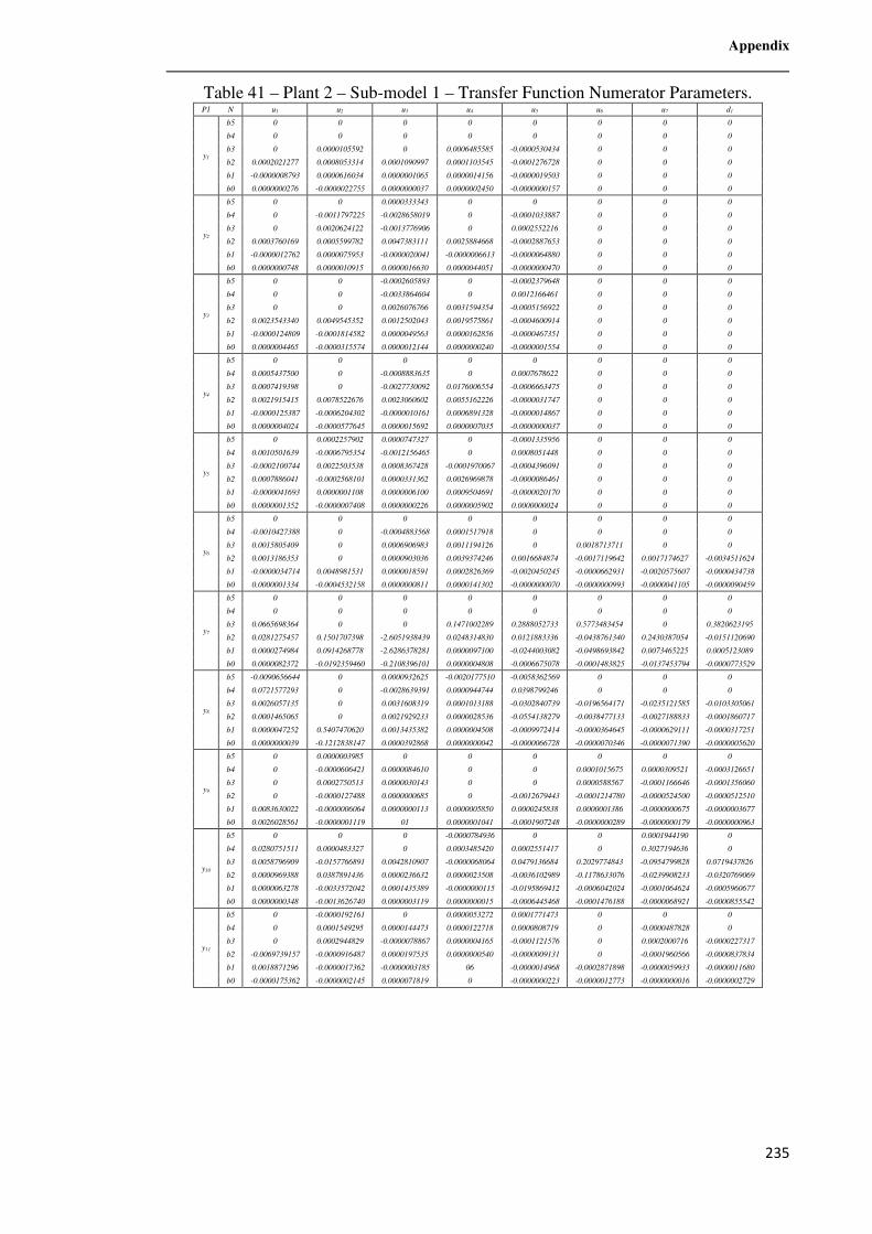
Appendix
235
Table 41 – Plant 2 – Sub-model 1 – Transfer Function Numerator Parameters. P1 N u1 u2 u3 u4 u5 u6 u7 d1
y1
b5 0 0 0 0 0 0 0 0
b4 0 0 0 0 0 0 0 0
b3 0 0.0000105592 0 0.0006485585 -0.0000530434 0 0 0
b2 0.0002021277 0.0008053314 0.0001090997 0.0001103545 -0.0001276728 0 0 0
b1 -0.0000008793 0.0000616034 0.0000001065 0.0000014156 -0.0000019503 0 0 0
b0 0.0000000276 -0.0000022755 0.0000000037 0.0000002450 -0.0000000157 0 0 0
y2
b5 0 0 0.0000333343 0 0 0 0 0
b4 0 -0.0011797225 -0.0028658019 0 -0.0001033887 0 0 0
b3 0 0.0020624122 -0.0013776906 0 0.0002552216 0 0 0
b2 0.0003760169 0.0005599782 0.0047383111 0.0025884668 -0.0002887653 0 0 0
b1 -0.0000012762 0.0000075953 -0.0000020041 -0.0000006613 -0.0000064880 0 0 0
b0 0.0000000748 0.0000010915 0.0000016630 0.0000044051 -0.0000000470 0 0 0
y3
b5 0 0 -0.0002605893 0 -0.0002379648 0 0 0
b4 0 0 -0.0033864604 0 0.0012166461 0 0 0
b3 0 0 0.0026076766 0.0031594354 -0.0005156922 0 0 0
b2 0.0023543340 0.0049545352 0.0012502043 0.0019575861 -0.0004600914 0 0 0
b1 -0.0000124809 -0.0001814582 0.0000049563 0.0000162856 -0.0000467351 0 0 0
b0 0.0000004465 -0.0000315574 0.0000012144 0.0000000240 -0.0000001554 0 0 0
y4
b5 0 0 0 0 0 0 0 0
b4 0.0005437500 0 -0.0008883635 0 0.0007678622 0 0 0
b3 0.0007419398 0 -0.0027730092 0.0176006554 -0.0006663475 0 0 0
b2 0.0021915415 0.0078522676 0.0023060602 0.0055162226 -0.0000031747 0 0 0
b1 -0.0000125387 -0.0006204302 -0.0000010161 0.0006891328 -0.0000014867 0 0 0
b0 0.0000004024 -0.0000577645 0.0000015692 0.0000007035 -0.0000000037 0 0 0
y5
b5 0 0.0002257902 0.0000747327 0 -0.0001335956 0 0 0
b4 0.0010501639 -0.0006795354 -0.0012156465 0 0.0008051448 0 0 0
b3 -0.0002100744 0.0022503538 0.0008367428 -0.0001970067 -0.0004396091 0 0 0
b2 0.0007886041 -0.0002568101 0.0000331362 0.0026969878 -0.0000086461 0 0 0
b1 -0.0000041693 0.0000001108 0.0000006100 0.0009504691 -0.0000020170 0 0 0
b0 0.0000001352 -0.0000007408 0.0000000226 0.0000005902 0.0000000024 0 0 0
y6
b5 0 0 0 0 0 0 0 0
b4 -0.0010427388 0 -0.0004883568 0.0001517918 0 0 0 0
b3 0.0015805409 0 0.0006906983 0.0011194126 0 0.0018713711 0 0
b2 0.0013186353 0 0.0000903036 0.0039374246 0.0016684874 -0.0017119642 0.0017174627 -0.0034511624
b1 -0.0000034714 0.0048981531 0.0000018591 0.0002826369 -0.0020450245 -0.0000662931 -0.0020575607 -0.0000434738
b0 0.0000001334 -0.0004532158 0.0000000811 0.0000141302 -0.0000000070 -0.0000000993 -0.0000041105 -0.0000090459
y7
b5 0 0 0 0 0 0 0 0
b4 0 0 0 0 0 0 0 0
b3 0.0665698364 0 0 0.1471002289 0.2888052733 0.5773483454 0 0.3820623195
b2 0.0281275457 0.1501707398 -2.6051938439 0.0248314830 0.0121883336 -0.0438761340 0.2430387054 -0.0151120690
b1 0.0000274984 0.0914268778 -2.6286378281 0.0000097100 -0.0244003082 -0.0498693842 0.0073465225 0.0005123089
b0 0.0000082372 -0.0192359460 -0.2108396101 0.0000004808 -0.0006675078 -0.0001483825 -0.0137453794 -0.0000773529
y8
b5 -0.0090656644 0 0.0000932625 -0.0020177510 -0.0058362569 0 0 0
b4 0.0721577293 0 -0.0028639391 0.0000944744 0.0398799246 0 0 0
b3 0.0026057135 0 0.0031608319 0.0001013188 -0.0302840739 -0.0196564171 -0.0235121585 -0.0103305061
b2 0.0001465065 0 0.0021929233 0.0000028536 -0.0554138279 -0.0038477133 -0.0027188833 -0.0001860717
b1 0.0000047252 0.5407470620 0.0013435382 0.0000004508 -0.0009972414 -0.0000364645 -0.0000629111 -0.0000317251
b0 0.0000000039 -0.1212838147 0.0000392868 0.0000000042 -0.0000066728 -0.0000070346 -0.0000071390 -0.0000005620
y9
b5 0 0.0000003985 0 0 0 0 0 0
b4 0 -0.0000606421 0.0000084610 0 0 0.0001015675 0.0000309521 -0.0003126651
b3 0 0.0002750513 0.0000030143 0 0 0.0000588567 -0.0001166646 -0.0001356060
b2 0 -0.0000127488 0.0000000685 0 -0.0012679443 -0.0001214780 -0.0000524500 -0.0000512510
b1 0.0083630022 -0.0000006064 0.0000000113 0.0000005850 0.0000245838 0.0000001386 -0.0000000675 -0.0000003677
b0 0.0026028561 -0.0000001119 01 0.0000001041 -0.0001907248 -0.0000000289 -0.0000000179 -0.0000000963
y10
b5 0 0 0 -0.0000784936 0 0 0.0001944190 0
b4 0.0280751511 0.0000483327 0 0.0003485420 0.0002551417 0 0.3027194636 0
b3 0.0058796909 -0.0157766891 0.0042810907 -0.0000068064 0.0479136684 0.2029774843 -0.0954799828 0.0719437826
b2 0.0000969388 0.0387891436 0.0000236632 0.0000023508 -0.0036102989 -0.1178633076 -0.0239908233 -0.0320769069
b1 0.0000063278 -0.0033572042 0.0001435389 -0.0000000115 -0.0195869412 -0.0006042024 -0.0001064624 -0.0005960677
b0 0.0000000348 -0.0013626740 0.0000003119 0.0000000015 -0.0006445468 -0.0001476188 -0.0000068921 -0.0000855542
y11
b5 0 -0.0000192161 0 0.0000053272 0.0001771473 0 0 0
b4 0 0.0001549295 0.0000144473 0.0000122718 0.0000808719 0 -0.0000487828 0
b3 0 0.0002944829 -0.0000078867 0.0000004165 -0.0001121576 0 0.0002000716 -0.0000227317
b2 -0.0069739157 -0.0000916487 0.0000197535 0.0000000540 -0.0000009131 0 -0.0001960566 -0.0000837834
b1 0.0018871296 -0.0000017362 -0.0000003185 06 -0.0000014968 -0.0002871898 -0.0000059933 -0.0000011680
b0 -0.0000175362 -0.0000002145 0.0000071819 0 -0.0000000223 -0.0000012773 -0.0000000016 -0.0000002729
Appendix
236
Table 42 – Plant 2 – Sub-model 1 – Transfer Function Denominator Parameters. P1 D u1 u2 u3 u4 u5 u6 u7 d1
y1
a5 0 1 0 1 1 0 0 0
a4 1 1.3507773846 1 2.0505333586 2.5459409282 0 0 0
a3 0.1389741430 1.1178069763 0.1278988268 0.2432815790 0.3156891595 0 0 0
a2 0.0012515215 0.2175232032 0.0021193276 0.0081242947 0.0086520647 0 0 0
a1 0.0000122512 0.0134499920 0.0000045124 0.0005295602 0.0000971112 0 0 0
a0 0.0000001026 0.0001699655 0.0000000735 0.0000079519 0.0000005114 1 1 1
y2
a5 0 1 1 0 0 0 0 0
a4 1 1.0321925954 16.8526437466 1 1 0 0 0
a3 0.2235842644 0.2887153565 7.0514227451 4.8607540969 0.2562881211 0 0 0
a2 0.0017588627 0.0092619440 0.1160946870 0.0891436860 0.0080387517 0 0 0
a1 0.0000445817 0.0005933967 0.0024769828 0.0082455499 0.0001178249 0 0 0
a0 0.0000001417 0.0000102265 0.0000387033 0.0001483415 0.0000003869 1 1 1
y3
a5 0 1 1 0 1 0 0 0
a4 1 1.3256143351 0.8770312258 1 0.8030191512 0 0 0
a3 0.3491007758 1.2309820553 0.1519942911 0.4178283212 0.2059811911 0 0 0
a2 0.0023434779 0.3371775272 0.0034117767 0.0099103709 0.0161713210 0 0 0
a1 0.0000482234 0.0198294963 0.0001494529 0.0000648156 0.0002609199 0 0 0
a0 0.0000003046 0.0002560674 0.0000022327 0.0000001167 0.0000007662 1 1 1
y4
a5 0 1 0 1 1 0 0 0
a4 1 1.6024388138 1 1.7965021318 0.1648570086 0 0 0
a3 0.1471268816 1.2565771703 0.1738836809 0.5288161072 0.0056337703 0 0 0
a2 0.0009963385 0.2304979257 0.0032637295 0.0541375393 0.0003659525 0 0 0
a1 0.0000188194 0.0108847753 0.0001191037 0.0008067949 0.0000060483 0 0 0
a0 0.0000001111 0.0001337089 0.0000017663 0.0000012991 0.0000000097 1 1 1
y5
a5 0 1 1 0 1 0 0 0
a4 1 0.7430327125 0.1489796612 0 0.1485903016 0 0 0
a3 0.0998199022 0.0852072696 0.0071800090 1 0.0087500236 0 0 0
a2 0.0008420395 0.0044157477 0.0001622476 0.1204811684 0.0005913750 0 0 0
a1 0.0000103375 0.0001862951 0.0000044619 0.0018161334 0.0000058419 0 0 0
a0 0.0000000765 0.0000028488 0.0000000411 0.0000020726 0.0000000325 1 1 1
y6
a5 0 0 1 0 1 1 1 1
a4 1 1 0.6473935561 1 1.2903523520 2.4446258986 1.4683268549 10.4732031134
a3 0.2653296007 1.5431967181 0.0773744616 1.5432376945 2.5683166616 1.0772813419 2.8901158270 3.7222645358
a2 0.0031078612 1.3283514917 0.0026113749 0.1361410524 0.9198969436 0.0510432746 1.0832577634 0.1236758551
a1 0.0000193241 0.3767487921 0.0000819485 0.0073189983 0.0148284997 0.0006577167 0.0195003172 0.0102044684
a0 0.0000001729 0.0062836388 0.0000010081 0.0000951577 0.0000035217 0.0000004053 0.0000402803 0.0001431268
y7
a5 1 1 0 0 1 1 0 1
a4 1.3572130005 1.8097388978 1 1 5.3083619025 5.0581347472 1 2.0503248828
a3 1.2342340899 3.8604394101 5.8838370829 2.2562370610 10.3018254782 9.6996882654 4.7959686546 6.8378238706
a2 0.1577333624 2.9585351944 15.1889006110 0.2490035716 6.3185649178 5.3682685821 9.4236350956 1.3305939516
a1 0.0003662304 1.6304808086 12.2535482201 0.0000581560 0.7981747255 0.5349731362 5.1716543055 0.0515429933
a0 0.0000466952 0.1847430953 1.3430591345 0.0000064175 0.0167372794 0.0014379936 0.4822115293 0.0025696256
y8
a5 1 1 1 1 1 1 1 1
a4 0.1503165495 5.2958977956 1.4426653376 0.0819735316 1.6707276449 0.7143893521 0.7118270698 0.6364857458
a3 0.0060416343 9.6051772750 1.9036848539 0.0189506739 1.2823644598 0.1869629710 0.1427399489 0.0773446327
a2 0.0003013495 12.4041520034 0.8948105947 0.0002445433 0.1213568826 0.0126794867 0.0091525279 0.0029083717
a1 0.0000071973 7.1742903199 0.0968367840 0.0000471779 0.0021935868 0.0003410102 0.0003667913 0.0002271625
a0 0.0000000114 0.7023874291 0.0021394427 0.0000000076 0.0000103854 0.0000209327 0.0000190806 0.0000029419
y9
a5 0 1 1 0 0 0 1 0
a4 0 1.0520707432 0.0846599356 0 0 1 0.4973705586 1
a3 0 0.2011216030 0.0059078738 1 0 0.1004218807 0.0404825688 0.0696313712
a2 0 0.0135481797 0.0003194767 0.0682934679 1 0.0011761851 0.0006461549 0.0028875427
a1 1 0.0005700614 0.0000081714 0.0126378766 0.1034187624 0.0000257065 0.0000139432 0.0001277360
a0 0.0012442849 0.0000067138 0.0000000235 0.0000088941 0.0011842736 0.0000002356 0.0000001644 0.0000015950
y10
a5 1 0 1 1 0 0 1 1
a4 0.3508745334 1 10.3303617886 0.0266592523 1 1 12.1942436420 3.3101140498
a3 0.0329630540 1.8072304391 1.3849122268 0.0067533245 2.2582640232 10.1444276417 4.0762547364 7.3266801993
a2 0.0004869378 2.0463462435 0.3502970090 0.0000904611 1.7336864338 1.4145982715 0.2805338782 0.9991431874
a1 0.0000342696 0.5705451687 0.0424946191 0.0000093553 0.2180957901 0.0213939878 0.0020121829 0.0420559587
a0 0.0000000216 0.0371332563 0.0000018047 0.0000000323 0.0050649862 0.0015783916 0.0000766420 0.0017131294
y11
a5 0 1 0 1 1 1 0 0
a4 0 0.8374120844 1 0.0205744522 0.1556860330 1.7553458934 1 1
a3 0 0.1807903308 0.1616483189 0.0041432406 0.0189629132 1.9200749947 0.2257513582 0.1612929715
a2 1 0.0083958996 0.7696995569 0.0000493362 0.0021255042 0.3222545834 0.0088047129 0.0073685733
a1 0.0022672061 0.0003959719 0.1208917214 0.0000030674 0.0000638827 0.0060404997 0.0000904162 0.0005383537
a0 0.0000110931 0.0000057115 0.0018330126 0.0000000167 0.0000003994 0.0000226508 0.0000000207 0.0000069499
Appendix
237
Table 43 – Plant 2 – Sub-model 2 – Transfer Function Numerator Parameters. P1 N u1 u2 u3 u4 u5 u6 u7 d1
y1
b5 0 0 0 0 0 0 0 0.0000083959
b4 0 0 0 0 0.0001646988 0.0001945853 0 0.0000245339
b3 0 0.0004579769 -0.0000755727 0 -0.0000415313 -0.0000363037 0 -0.0000077387
b2 0.0000266875 -0.0000120663 -0.0000852804 0.0013504814 0.0000027681 0.0000025809 0.0004399067 -0.0000030015
b1 0.0000091466 0.0000010903 0.0000266649 -0.0002071391 -0.0000005413 -0.0000003578 -0.0002935855 -0.0000000350
b0 -0.0000000437 -0.0000000313 -0.0000000342 0.0000024410 04 0.0000000020 -0.0000008720 -0.0000000022
y2
b5 0 0 0 0 0.0000445325 0 0 0
b4 0 0 0 0 0.0002779238 0.0002916357 0 0.0003070780
b3 0.0010106250 -0.0015726386 0 0 -0.0001881113 0.0004773534 0.0001881203 0.0000832513
b2 0.0012054628 0.0028013185 0.0005213455 -0.0190835358 -0.0000545334 -0.0003711473 0.0000794712 -0.0001363461
b1 0.0002495583 0.0008950736 0.0001495288 -0.0026425631 -0.0000031566 -0.0000514493 -0.0001490255 -0.0000003114
b0 0.0000004676 0.0000153172 -0.0000000312 -0.0000021044 -0.0000000027 -0.0000013860 -0.0000004961 -0.0000002835
y3
b5 0 -0.0004267206 0 0 0 0 0 0
b4 0 -0.0087536959 0 0 0.0001429595 0.0004666645 0.0001485433 -0.0004235691
b3 0 0.0115364458 -0.0045768795 -0.0034364386 0.0012508687 0.0026747842 0.0009805454 0.0020048723
b2 0 -0.0011981122 0.0059345573 -0.0020279844 -0.0011416812 -0.0025076291 -0.0009347483 -0.0019532109
b1 -0.0035877559 0.0000207564 0.0013661854 -0.0000033794 -0.0000266400 -0.0000563681 -0.0000240001 -0.0001205239
b0 0.0064160140 -0.0000040714 0.0000004825 -0.0000017302 -0.0000001717 -0.0000003426 -0.0000000903 -0.0000033023
y4
b5 0 -0.0004195370 0 0 0 0 0 0
b4 0 -0.0072930566 0 0 0 0 0 0
b3 0 0.0083951082 0 -0.0205209457 0 0 0 0
b2 0 -0.0011352139 -0.0146373318 -0.0045843759 0 0 0 -0.0008417440
b1 -0.0045614631 0.0000023551 0.0163370273 -0.0000060247 -0.0010914736 -0.0006197362 -0.0009954657 0.0000003341
b0 0.0047473950 -0.0000037782 0.0000209701 -0.0000015374 -0.0000004490 -0.0000000668 -0.0000005434 -0.0000013480
y5
b5 0 -0.0005394863 0 0 0 0 0 0
b4 0 -0.0016683556 0 0 0 0 0 0
b3 0 0.0018487474 0 -0.0031201381 0.0016208241 0.0003430117 0.0014969053 0
b2 0 -0.0002780772 0 -0.0011419668 -0.0014593569 -0.0005164719 -0.0014175673 0.0007745400
b1 -0.0027651123 -0.0000023218 -0.0019280963 -0.0000045661 0.0000013119 0.0000004274 0.0000013405 -0.0009032513
b0 0.0017894571 -0.0000009383 0.0011135411 -0.0000003297 -0.0000003316 -0.0000001217 -0.0000002536 -0.0000028607
y6
b5 0 0 -0.0000211806 0 0 0 0 0
b4 0 -0.0015753530 -0.0011157351 0 0 -0.0000468704 0 0
b3 0 0.0023805120 0.0014797675 -0.0070229353 0 0.0008365529 0 0.0005070473
b2 0.0037396289 -0.0002208452 0.0000065378 -0.0006138597 0.0008631190 -0.0006965313 0.0005662017 -0.0004538986
b1 0.0001189712 0.0000042213 0.0000056547 -0.0000056215 -0.0012233663 -0.0000090619 -0.0004782242 0.0000013788
b0 0.0000014600 -0.0000006401 02 -0.0000004919 -0.0000016283 -0.0000000361 -0.0000002515 -0.0000010479
y7
b5 -0.0061526846 0 0 0 0 0 0 0
b4 0.0296668498 0 0 0 0 0 0 0
b3 0.0008082933 0 0 0 0 0 0 0.2734867646
b2 0.0000636204 0.1321910413 -4.2785460923 -1.0846738670 0.5091044695 0.3581208846 0.4622904385 0.1156658241
b1 0.0000017696 -0.0225098633 -4.3044072055 -1.9576299851 -0.0203533212 -0.0387203183 0.0129070084 -0.0354414360
b0 07 -0.0002223130 -0.3355447832 -0.2722545938 -0.0417693541 -0.0324541603 -0.0314011268 -0.0012892473
y8
b5 0 0 0 0.0000817090 0 0.0003981585 0 0
b4 0.0050271593 -0.0055637836 0 0.0000344088 0.0148250023 0.0084741196 0 0
b3 0.0497708158 0.0147875692 0.0002901979 -0.0000209241 -0.0175359739 -0.0100225475 0 -0.0010680956
b2 0.0072378057 -0.0036541940 0.0003623077 -0.0000027475 -0.0002701752 -0.0005796065 0.0517751917 -0.0064951298
b1 0.0002707512 0.0000315369 0.0000163354 -0.0000004381 -0.0000185236 -0.0000148529 -0.1099601828 -0.0000563924
b0 0.0000007591 -0.0000116269 0.0000062830 -0.0000000115 -0.0000001020 -0.0000008944 -0.0089639132 -0.0000007683
y9
b5 0 -0.0001188010 0 0 0 0.0012065733 0 0
b4 0 -0.0240690388 0 0 0 0.0004719949 0 0
b3 0 0.0200082325 0 0 0 -0.0004660992 0 0
b2 -0.0002016495 -0.0028511082 0 -0.0000038731 -0.0002153636 -0.0000592822 -0.0001977354 -0.0002283097
b1 0.0010289943 0.0000599742 0.0000166552 -0.0000000435 -0.0000460999 -0.0000003429 -0.0000350732 -0.0000004358
b0 0.0013293070 -0.0000107140 -0.0000002102 -06 0.0000000132 -04 0.0000000127 -0.0000003504
y10
b5 -0.0040354413 0 0 0 0 0.0000614155 0.0000286214 0
b4 0.0322028014 -0.0068020531 0 0.0000355112 0 0.0362719151 11.6760861163 0.0001643220
b3 0.0167444308 0.0239450464 0.0007411858 0.0025927586 0.3243103791 0.0019762885 -2.8697500175 0.0240872290
b2 0.0011291981 -0.0061656389 0.0004712910 -0.0009114023 0.3059953575 -0.0222968342 -1.0800340567 -0.0136841675
b1 0.0000027097 -0.0000845970 0.0000043797 -0.0000040963 -0.3848958333 -0.0011960293 -0.0436156677 -0.0035952072
b0 0.0000001239 -0.0000294108 0.0000000318 0.0000001074 -0.0292012080 -0.0000163213 -0.0000436047 -0.0001918816
y11
b5 0 0 0 0 0 0 0 0
b4 0 0.0000789961 0 0 0 0 0 0.0001827257
b3 0 0.0001541394 0.0000200309 0 0 0.0003744995 0 -0.0002969679
b2 0 -0.0000991345 -0.0000001390 0 0 -0.0004501734 0 -0.0000682615
b1 0.0012500148 0.0000001303 0.0000000686 -0.0000089236 -0.0005127704 -0.0000065300 -0.0005042485 -0.0000001914
b0 0.0000008153 -0.0000003078 -05 -0.0000000353 0.0000001098 -0.0000000174 -0.0000000136 -0.0000000119
Appendix
238
Table 44 – Plant 2 – Sub-model 2 – Transfer Function Denominator Parameters. P1 D u1 u2 u3 u4 u5 u6 u7 d1
y1
a5 1 1 0 0 1 1 0 1
a4 0.9022658577 1.4167540291 0 0 0.1402274786 0.2397707429 1 0.3139954487
a3 0.3173851327 0.1144181768 1 0 0.0156038975 0.0114872846 21.6057345836 0.0276853766
a2 0.0255477291 0.0076090816 0.1329340032 1 0.0018798958 0.0021917784 2.5612733951 0.0008726327
a1 0.0002253713 0.0002574887 0.0018370107 0.0017388599 0.0000294349 0.0000166053 0.0435563322 0.0000205078
a0 0.0000002662 0.0000066296 0 0.0000747768 0.0000000080 0.0000001465 0.0001119346 0.0000003009
y2
a5 0 0 1 1 1 0 0 0
a4 1 1 1.4609958758 3.8032430285 0.5491104364 1 0 1
a3 0.4897330091 1.0653609121 0.9353149427 13.3563647566 0.0825374409 0.3531747536 1 0.1732826433
a2 0.0563708683 0.3286032327 0.1610617195 2.0530141748 0.0042803077 0.0346824855 0.2093974551 0.0053417270
a1 0.0006991356 0.0112487072 0.0023945335 0.0328002825 0.0000540074 0.0010997108 0.0035888443 0.0003592680
a0 0.0000071343 0.0000907810 0.0000000301 0.0000197011 0.0000000388 0.0000113428 0.0000142317 0.0000053242
y3
a5 0 1 1 0 0 0 0 0
a4 0 1.1493784228 3.8886158584 1 1 1 1 1
a3 0 0.3309695649 2.2749239139 0.3922966508 0.3363296518 0.3252537675 0.3434637049 0.4009238735
a2 1 0.0104316017 0.2865644933 0.0070564978 0.0114593500 0.0108665445 0.0122610604 0.0251294677
a1 0.3449236252 0.0010461294 0.0042584574 0.0003343929 0.0001576989 0.0001448445 0.0001545607 0.0008157440
a0 0.0048397043 0.0000129245 0.0000023299 0.0000052884 0.0000006354 0.0000005570 0.0000003900 0.0000074581
y4
a5 0 1 0 1 1 1 1 1
a4 0 1.0201588062 1 3.5714659176 0.7507242908 0.6735141682 0.8286698481 1.3977570748
a3 0 0.1800965935 12.2595753515 0.5535729355 0.8632976847 0.7621399370 0.9532127408 0.1874560514
a2 1 0.0072207071 1.9553151965 0.0088355212 0.1183576305 0.1026561292 0.1330434304 0.0049621452
a1 0.2091556904 0.0005193761 0.0313827594 0.0001892288 0.0017253097 0.0014724350 0.0019524728 0.0002989867
a0 0.0026829128 0.0000057891 0.0000371099 0.0000026043 0.0000017616 0.0000009751 0.0000023834 0.0000043654
y5
a5 0 1 0 0 1 1 1 1
a4 0 0.5687713341 0 1 1.4699109337 0.8346571866 1.7451058141 1.3745938232
a3 0 0.0801955458 0 0.1270054779 0.1624665830 0.0893185832 0.1919656249 2.0351323311
a2 1 0.0034060145 1 0.0024742197 0.0023563156 0.0012771814 0.0027367182 0.2143254141
a1 0.1579902477 0.0002111567 0.1257493303 0.0000417821 0.0000380656 0.0000217722 0.0000348602 0.0035846856
a0 0.0018123064 0.0000019125 0.0017827840 0.0000005723 0.0000004720 0.0000002623 0.0000004398 0.0000099388
y6
a5 0 1 1 1 1 0 0 0
a4 1 0.9698714976 0.5954991382 2.7477883929 1.3258623878 1 0 1
a3 1.0553524202 0.3615643339 0.0180458683 0.2882374723 2.5555033053 0.4453838244 1 0.3692358911
a2 0.0437484849 0.0105674664 0.0023318739 0.0061063638 0.9265907561 0.0122280387 0.4491529310 0.0083144703
a1 0.0009137417 0.0010295630 0.0000377092 0.0002323759 0.0156587066 0.0001133455 0.0073182757 0.0008544210
a0 0.0000024354 0.0000143565 0.0000000180 0.0000031408 0.0000252732 0.0000003001 0.0000069820 0.0000138852
y7
a5 1 1 0 1 0 0 0 1
a4 0.2516606967 3.0552345950 1 4.7678810673 1 1 1 4.4033571585
a3 0.0075797767 3.3615651340 5.5873022701 17.9036346473 4.5314974527 4.6258713970 4.5222249435 10.1203516285
a2 0.0005472978 2.8085427909 14.2614550266 37.2565227113 8.9445384355 9.0630227573 9.0057115879 8.9918088444
a1 0.0000115863 0.4171279077 11.5592086229 29.3734958867 5.1306521332 5.0596839112 5.2583191917 1.4625895061
a0 0.0000000266 0.0037049659 1.2631255000 2.6897968259 0.5015135716 0.4870742807 0.5131920208 0.0371892621
y8
a5 1 1 1 1 1 1 1 1
a4 2.9875467844 1.3903808122 0.5582292966 0.4969747432 1.9834821136 1.8095909167 6.3309963745 1.7812822383
a3 0.7203395005 1.0577258493 1.2018544174 0.0783270383 0.2571980245 0.2945232188 14.3930697228 1.5055856751
a2 0.0600511505 0.1210196845 0.1666989405 0.0098272301 0.0056938940 0.0137248879 17.4986753520 0.1692941205
a1 0.0017076050 0.0038189527 0.0233805869 0.0005700999 0.0002428236 0.0004345511 3.2100470531 0.0013953628
a0 0.0000030964 0.0003553788 0.0021261344 0.0000118567 0.0000013145 0.0000163452 0.1418164524 0.0000203861
y9
a5 0 1 0 0 1 1 1 0
a4 0 32.6992877304 0 1 1.2628323939 0.2147019182 1.4360957771 1
a3 0 4.7137164960 1 0.0818784103 0.3226717796 0.0132708183 0.3421977710 0.1041241910
a2 1 0.2033522271 0.1246992002 0.0019432189 0.0225012340 0.0002018663 0.0227273771 0.0026059392
a1 0.1386706609 0.0172574502 0.0000159029 0.0000193616 0.0002415064 0.0000013049 0.0002427179 0.0001606628
a0 0.0012259182 0.0002098152 0.0000019830 0.0000000088 0.0000008700 0.0000000016 0.0000007680 0.0000016400
y10
a5 1 1 1 0 1 1 1 0
a4 0.6778925912 1.2489268998 0.4669077588 1 10.1678115424 2.8874563752 456.6826204285 1
a3 0.1034473339 1.5270514898 1.5154201059 5.6154548676 26.7957935483 2.4961804940 178.6062121511 2.7366984250
a2 0.0044574198 0.2505126585 0.1507556211 0.9081818579 32.8319818511 0.3885616676 18.4290042430 0.8939480133
a1 0.0000142108 0.0122712014 0.0014157508 0.0001173394 6.1339980248 0.0145190679 0.5019425324 0.0952741995
a0 0.0000005982 0.0008566492 0.0000002274 0.0000153144 0.2456834863 0.0001769231 0.0004975308 0.0031165035
y11
a5 1 1 1 0 1 0 1 1
a4 0.9049849117 0.4975606977 0.1427663052 0 1.2602621676 1 1.5926543722 0.3722848156
a3 0.6372676372 0.0997878349 0.0046206328 1 1.6580641686 0.1926480226 2.1277577405 0.0373841108
a2 0.0849876385 0.0028738145 0.0005153596 0.1211725019 0.2558788680 0.0051261064 0.3310813409 0.0006396440
a1 0.0013767782 0.0003055812 0.0000032551 0.0024834831 0.0037105051 0.0000466205 0.0048703332 0.0000075642
a0 0.0000040080 0.0000039898 0.0000000085 0.0000015873 0.0000007325 0.0000000730 0.0000022506 0.0000000846
Appendix
239
Table 45 – Plant 2 – Sub-model 3 – Transfer Function Numerator Parameters. P1 N u1 u2 u3 u4 u5 u6 u7 d1
y1
b5 0 0 0 0 0 0 0 0
b4 0 0 0 0 0 0 0 0
b3 0 0.0000175239 0 0 -0.0000333074 -0.0000372682 0.0000319584 0
b2 0 0.0000005680 0 0 -0.0000392829 -0.0000228452 -0.0000190525 0.0010899294
b1 0.0000665099 0.0000000178 0.0001262609 0.0000331833 -0.0000097290 -0.0000009110 -0.0000011602 -0.0002110223
b0 -0.0000005132 -05 0.0000175729 -0.0000002939 -0.0000000461 -0.0000000067 0.0000000017 0.0000013831
y2
b5 0 0 0 0 0 0 0 0
b4 0 0 0 0 0 0 0 0
b3 -0.0016103813 0.0004405647 0 0 0 0 0 -0.0003027473
b2 0.0019083898 -0.0000036305 0.0004840073 0.0058592297 0 -0.0008393909 0 -0.0000034523
b1 0.0000090411 0.0000016609 0.0000071425 -0.0000074492 -0.0003246591 -0.0002703587 -0.0001866340 -0.0000047599
b0 -0.0000000990 -0.0000000097 0.0000000210 0.0000000261 -0.0000004223 -0.0000008478 0.0000006028 0.0000000048
y3
b5 0 0 0 0 0 0 0 0
b4 0 0 0 0 0 0 0 -0.0002043482
b3 0 0 0.0052484237 0 0 0 0 -0.0022874121
b2 0.0061340698 0 -0.0095451519 0 0 0 0 -0.0010612134
b1 0.0000140237 -0.0000801431 0.0061282710 0.0089135247 -0.0021110274 -0.0020838636 -0.0047037902 -0.0000057284
b0 -0.0000001858 -0.0000004924 -0.0000033103 0.0051078944 0.0000005953 -0.0000009606 -0.0000003227 -0.0000000687
y4
b5 0 0 0 0 0 0 0 0.0008202328
b4 -0.0030490538 0 0 0 -0.0002678044 0 0 0.0001039400
b3 -0.0030681869 0 0 0 -0.0014278452 0 0 -0.0007550896
b2 0.0029098675 -0.0000196715 0.0030428617 0 -0.0000045963 0 0 -0.0000441384
b1 0.0000046170 -0.0000016641 0.0055855208 0.0076101457 -0.0000020413 -0.0009716500 -0.0011924207 -0.0000042160
b0 -0.0000000679 -0.0000000313 0.0001668090 -0.0000106677 -0.0000000064 -0.0000005271 0.0000003736 -0.0000000104
y5
b5 0 0 0 0 0 0 -0.0002883790 0
b4 0 0 0 0 0.0023714099 0.0027427250 0.0009104693 0
b3 0 0 0 0.0012924335 -0.0013684009 -0.0015221134 -0.0006148573 0.0017498474
b2 -0.0156977637 0.0017547171 0.0026802565 0.0006677549 0.0000100803 -0.0000762867 -0.0000342308 -0.0007545139
b1 0.0007754898 -0.0003634464 0.0000078206 0.0000115395 -0.0000047640 -0.0000047937 -0.0000039121 0.0000023857
b0 0.0029331458 -0.0000018932 0.0000000138 -0.0000000302 0.0000000017 0.0000000020 -0.0000000012 -0.0000001466
y6
b5 0 0 0 0 0 0 0 0
b4 0 0 0 0 0 0 0 0
b3 0 0 0 0 0 0 0.0002852926 0
b2 0.0033199036 0.0015373411 -0.0035800828 0.0004254101 0 0 0.0001025960 0
b1 0.0001184041 -0.0001885723 0.0020361844 0.0000226659 -0.0007031823 -0.0008220264 -0.0003432217 -0.0007390235
b0 -0.0000003228 0.0000005544 0.0000024102 -0.0000003319 -0.0000000609 -0.0000000370 -0.0000002025 0.0000023095
y7
b5 0 0 0 0 0 0 0 0
b4 0 0 0 0 0 0 0 0
b3 0.0970009299 0 0 0 0 0.7354469313 0.2528129462 0
b2 0.0422178516 0.0224736172 -1.9154960249 0 1.2772605815 0.0526000159 0.0260166174 0.5305425938
b1 0.0000453325 0.0277576844 -1.9601720792 25.3117557456 -0.0605915309 -0.1091498343 -0.0239855565 0.2047934264
b0 0.0000115303 -0.0066741618 -0.1568666168 5.3411632263 -0.1313758473 -0.0060268188 -0.0005026206 -0.0859792667
y8
b5 0 0 0 0 0 -0.0083261013 0 0
b4 0.0718807243 0 0 0.0000748122 0 0.6090570143 0.1162237335 0
b3 0.1855911945 0.0064947786 0.0023654778 0.0000211687 0 -0.6757156899 -0.1278380390 -0.0296744462
b2 0.0248093522 0.0152618232 0.0000120402 0.0000002983 0.0693444306 0.0002008011 -0.0003207655 -0.0183699815
b1 0.0001961484 -0.0073695112 0.0000080242 0.0000000788 -0.1007077374 -0.0016791518 -0.0004219872 -0.0004884064
b0 0.0000019400 -0.0000717456 -0.0000000079 02 -0.0000599623 -0.0000019481 -0.0000017881 -0.0000229578
y9
b5 0 0 0 0 0 0 0 0
b4 0 0 0 0 0 0 0 0
b3 0 0 0 0 0 -0.0001405224 0 0
b2 -0.0275423287 0.0005879621 0.0000007831 0.0000000252 0 -0.0000556917 0 0
b1 0.0047213447 -0.0000178545 0.0000000051 -0.0000000418 -0.0002381400 -0.0000034266 -0.0001410354 -0.0001006227
b0 -0.0000441181 0.0000017793 04 0.0000000012 0.0000010185 0.0000000137 0.0000002612 0.0000008231
y10
b5 0 -0.0000594176 0 0 0 0.0002954625 0 0
b4 0.0664476649 -0.0013910804 -0.0023953517 0 0 0.0629222633 0.0000711968 0
b3 0.2247552834 0.0045989169 0.0023891502 -0.0042855275 0.2203472006 -0.0070594978 0.0294013806 0.0348918527
b2 0.0016409563 0.0027479811 0.0008943826 0.0012466645 0.1562178688 -0.0298472639 0.0002873347 -0.0086190178
b1 0.0001930643 -0.0014772641 0.0005389002 0.0000429309 -0.2299438601 -0.0014515736 -0.0084886602 -0.0128737798
b0 0.0000010602 -0.0004231430 -0.0000000678 0.0000000986 -0.0165988601 -0.0000014236 -0.0004700969 -0.0006437994
y11
b5 0 0 0 0 0 0 0 0
b4 0 0 0 0 0 0 0 0
b3 0 0 0 -0.0001029896 0 0 0 -0.0005288331
b2 0.0027001630 0.0014687961 0 -0.0000041810 0 0 0.0048142306 -0.0000023269
b1 0.0000076554 -0.0003705849 01 0.0000014123 -0.0004753838 -0.0013369067 -0.0012253774 -0.0000019404
b0 -0.0000000454 0.0000002433 0 -0.0000000094 -0.0000002590 0.0000002482 0.0000115119 -0.0000000017
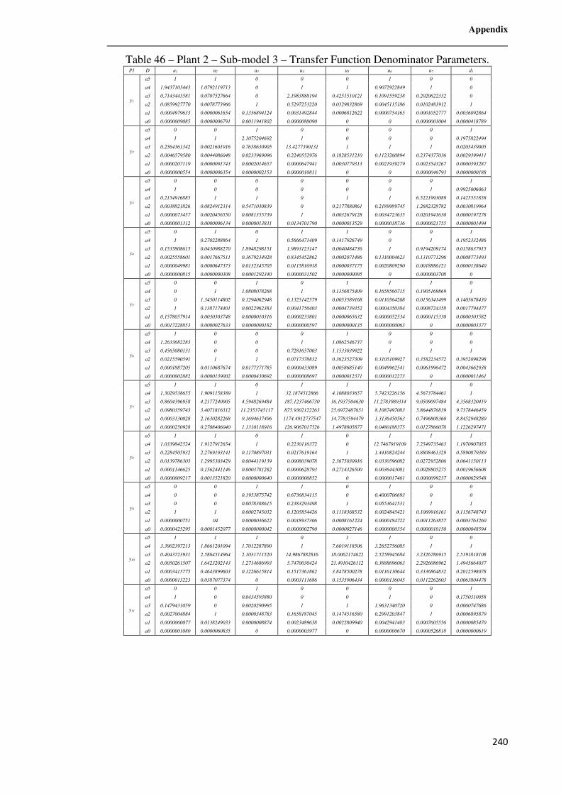
Appendix
240
Table 46 – Plant 2 – Sub-model 3 – Transfer Function Denominator Parameters. P1 D u1 u2 u3 u4 u5 u6 u7 d1
y1
a5 1 1 0 0 0 1 0 0
a4 1.9437103443 1.0792119713 0 1 1 0.9072922849 1 0
a3 0.7143443581 0.0707527664 0 2.1983888194 0.4251510121 0.1091559238 0.2020622332 0
a2 0.0859927770 0.0078773966 1 0.5297253220 0.0329832869 0.0045115186 0.0102481912 1
a1 0.0004979633 0.0000061654 0.1356894124 0.0031492844 0.0006812622 0.0000754165 0.0001052777 0.0036092864
a0 0.0000009085 0.0000006791 0.0011941802 0.0000088090 0 0 0.0000001004 0.0000418789
y2
a5 0 0 1 0 0 0 0 1
a4 1 1 2.1075204692 1 0 0 0 0.1975822494
a3 0.2564361342 0.0021601916 0.7658630905 13.4277390131 1 1 1 0.0205439005
a2 0.0046579580 0.0044086048 0.0233969096 0.2240552976 0.1828531210 0.1123260894 0.2374377036 0.0029399411
a1 0.0000207119 0.0000091743 0.0002014657 0.0000647941 0.0030779313 0.0021939279 0.0023543267 0.0000393287
a0 0.0000000554 0.0000006354 0.0000002153 0.0000010811 0 0 0.0000046793 0.0000000188
y3
a5 0 0 0 0 0 0 0 1
a4 1 0 0 0 0 0 1 0.9925006063
a3 0.2154916885 1 1 0 1 1 6.5221993089 0.1425551858
a2 0.0038821826 0.0824912314 0.5471030839 0 0.2177880861 0.2189989745 1.2682328782 0.0030819964
a1 0.0000073457 0.0020456550 0.0081355739 1 0.0032679128 0.0034723635 0.0201941630 0.0000197278
a0 0.0000001312 0.0000006134 0.0000013831 0.0134701790 0.0000013529 0.0000018736 0.0000021755 0.0000001494
y4
a5 0 1 0 1 1 0 0 1
a4 1 0.2702288864 1 0.5666471409 0.1417926749 0 1 0.1952332486
a3 0.1535808615 0.0430988270 1.8948298151 1.9893123147 0.0040484736 1 0.9194209174 0.0158637915
a2 0.0025558601 0.0017667511 0.3679234928 0.8345452862 0.0002071486 0.1310004623 0.1310771296 0.0008773493
a1 0.0000049981 0.0000647373 0.0132345705 0.0115816918 0.0000037175 0.0020809290 0.0018886121 0.0000138640
a0 0.0000000815 0.0000000308 0.0001292340 0.0000031502 0.0000000095 0 0.0000003708 0
y5
a5 0 0 1 0 1 1 1 0
a4 0 1 1.0808078268 1 0.1356875409 0.1658560715 0.1905169869 1
a3 0 1.3450114802 0.1294062948 0.1325142579 0.0053589168 0.0110564208 0.0156341499 0.1405678430
a2 1 0.1387174401 0.0022962383 0.0041750403 0.0004739352 0.0004350384 0.0008724358 0.0017794477
a1 0.1578057914 0.0030303748 0.0000010316 0.0000233801 0.0000065632 0.0000052534 0.0000115330 0.0000303582
a0 0.0017228853 0.0000027633 0.0000000182 0.0000000597 0.0000000135 0.0000000063 0 0.0000003377
y6
a5 1 0 0 0 1 0 0 0
a4 1.2633682283 0 0 1 1.0862546737 0 0 0
a3 0.4565080131 0 0 0.7281657003 1.1533039922 1 1 1
a2 0.0215590591 1 1 0.0717378832 0.3623527309 0.3105109927 0.3582234572 0.3952098298
a1 0.0001887205 0.0110687674 0.0177371785 0.0000433089 0.0058685140 0.0049962541 0.0061996472 0.0043662938
a0 0.0000002882 0.0000139002 0.0000430692 0.0000008697 0.0000012371 0.0000012273 0 0.0000011461
y7
a5 1 1 0 1 1 1 1 0
a4 1.3029538655 1.9091158389 1 32.1874512866 4.1088033657 5.7423226156 4.5673784461 1
a3 0.8604396958 4.2177240905 4.5948269484 187.1237466730 16.1937504630 11.2783989314 9.0509097484 4.3568320419
a2 0.0980359743 3.4071816312 11.2353745117 875.9302122263 25.6972487651 8.1087497083 5.8644876839 9.7378446459
a1 0.0003130028 2.1630282268 9.1694637496 1174.4912737547 14.7783594479 1.3136450563 0.7496808360 8.8452948280
a0 0.0000250928 0.2708406040 1.1310118916 126.9067017526 1.4978805877 0.0480188375 0.0127866078 1.1226297471
y8
a5 1 1 0 1 0 1 1 1
a4 1.0339842524 1.9127912654 1 0.2230116372 0 12.7467919109 7.2549735463 1.1970907055
a3 0.2284505932 2.2769193141 0.1170897031 0.0217619164 1 1.4410824244 0.8808461329 0.5890879389
a2 0.0139786303 1.2995303429 0.0044119139 0.0008039078 2.3675030916 0.0330596082 0.0272952806 0.0641150113
a1 0.0001146625 0.1562441146 0.0003781282 0.0000628793 0.2714326500 0.0036443081 0.0028805275 0.0019656608
a0 0.0000009217 0.0013521820 0.0000000640 0.0000000852 0 0.0000017461 0.0000099237 0.0000629548
y9
a5 0 0 1 1 0 1 0 0
a4 0 0 0.1953875742 0.6736834115 0 0.4000706693 0 0
a3 0 0 0.0078388615 0.2383293498 1 0.0553641531 1 1
a2 1 1 0.0002745032 0.1205854426 0.1118368532 0.0024845421 0.1069916161 0.1156748743
a1 0.0000000751 04 0.0000036622 0.0018937306 0.0008161224 0.0000184722 0.0011263857 0.0003763260
a0 0.0000425295 0.0001452077 0.0000000042 0.0000002790 0.0000027146 0.0000000354 0.0000010150 0.0000048594
y10
a5 1 1 1 0 1 1 0 0
a4 3.3902397213 1.8661201094 1.7012287890 1 7.6019118506 3.2652756085 1 1
a3 0.4043723931 2.5864514964 2.1031711520 14.9867882816 18.0062174622 2.5258945684 3.2326786915 2.5191818108
a2 0.0050261507 1.6423202143 1.2714686993 5.7470030424 21.4910426112 0.3688696063 2.2926086962 1.4945664037
a1 0.0003415775 0.4643899603 0.1226615814 0.1517361862 3.8478500278 0.0116130644 0.3336864832 0.2012598078
a0 0.0000013223 0.0387077374 0 0.0003111686 0.1535906434 0.0000136045 0.0112262603 0.0063804478
y11
a5 0 0 1 0 0 0 0 1
a4 1 0 0.0434593880 0 0 1 0 0.1750310058
a3 0.1479431059 0 0.0020290995 1 1 1.9631340720 0 0.0060747686
a2 0.0027004884 1 0.0000348783 0.1658187045 0.1474516580 0.2991203847 1 0.0006895879
a1 0.0000060077 0.0138249033 0.0000008874 0.0023489638 0.0022809940 0.0042941403 0.0007605556 0.0000085470
a0 0.0000001080 0.0000060835 0 0.0000003977 0 0.0000000670 0.0000526818 0.0000000619
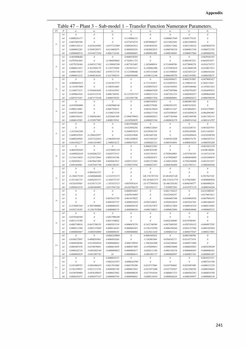
Appendix
241
Table 47 – Plant 3 – Sub-model 1 – Transfer Function Numerator Parameters. P1 N u1 u2 u3 u4 u5 u6 u7 d1
y1
b5 0 0 0 0 0 0 0 0
b4 0.0088265377 0 0 0.1148066535 0 -0.0000617049 0.0056779129 0
b3 0.0032902506 0 0 0.0774254574 0.0078000437 0.0114822949 -0.0012490954 0
b2 0.0003150114 -0.0258105881 -0.0757127689 0.0082045612 -0.0019656391 -0.0026171062 -0.0031390142 -0.0029029759
b1 0.0000041281 0.5849528973 0.0116802676 0.0000282916 -0.0038822835 -0.0048766530 -0.0000017349 -0.0000723765
b0 0.0000000510 -0.0149272364 0.0061516246 0.0000006085 0.0000001888 -0.0000100091 -0.0000027660 -0.0000069582
y2
b5 -0.0039096482 0 0 0.0000258205 0 0 0 -0.0038565107
b4 0.0707643044 0 -0.1960958602 0.7428811725 0 0 0.0003487225 0.0642953837
b3 0.0578356360 -0.0493317362 -0.1388095299 0.9875932485 1.1629408914 0.5514690706 0.0578688278 -0.0316719715
b2 0.0068412453 0.5632949179 0.1393578490 1.2819935417 -0.3309061086 -0.2555883639 -0.0130848198 -0.0149671831
b1 0.0000518072 1.0262823462 0.8795715778 0.1125098406 -0.3955333648 -0.1413999845 -0.0223051227 -0.0004341016
b0 0.0000013232 0.0400236244 0.1017949219 0.0002946908 -0.0306112196 -0.0066498750 -0.0021445081 -0.0000348271
y3
b5 0 0 0 0 0 0.0010956671 0.0002767085 -0.0079085427
b4 -0.0009043812 0 -0.2033617575 0 0.1731163471 0.2145907014 0.1398816110 0.1602123021
b3 -0.1103957089 0 0.1982914405 0 -0.0298955412 -0.0345505893 -0.0497696964 -0.1070915423
b2 0.3100273231 0.5916043620 0.1365419591 0 -0.0806847628 -0.0977007066 -0.0502784387 -0.0264095833
b1 0.3099043910 0.6165535354 0.0081760591 16.3121853737 -0.0069315319 -0.0073931353 -0.0026991857 -0.0009044360
b0 0.0207475447 -0.0671774358 0.0000559529 1.9215007790 -0.0000037294 -0.0000008061 -0.0000020235 -0.0000590189
y4
b5 0 0 0 0 -0.0003545851 0 0.0002887180 0
b4 -0.0195094886 0 -0.2605066146 0 0.0801275690 0.0983953472 0.0697419224 0
b3 0.0909114681 0 0.0467562611 0 -0.0034139430 0.0083311167 -0.0230844811 0.0321276965
b2 0.0070711099 0 0.1390273359 0 -0.0564177330 -0.0710786167 -0.0330389274 -0.0642091967
b1 0.0001939331 2.3949561661 0.0220481508 31.9946799923 -0.0040492612 -0.0077383904 -0.0021999788 -0.0017565333
b0 0.0000147083 -0.3220977687 0.0008159501 4.6345899078 -0.0000051504 -0.0000016178 -0.0000543340 -0.0001414797
y5
b5 0 0 0 0.0015950460 0 0 0 0
b4 0 0 0 0.6325692292 -0.0002152645 0 0.0232248731 -0.0032027931
b3 -1.4331843106 0 0 0.2048819219 0.0358501529 0 0.0202420286 0.0111445825
b2 2.0498547018 0.2388432977 0 0.0169193848 0.0032407326 0 -0.0392489436 -0.0228388709
b1 0.0000249920 -0.0271222814 -2.3662893349 0.0012400850 -0.0333401267 -0.0465852208 0.0000374170 -0.0005267533
b0 0.0014582277 -0.0011019907 2.3908854272 0.0000479255 -0.0000261511 -0.0003934891 -0.0000650229 -0.0000585280
y6
b5 0 0 0 0 0.0004255303 0 0 -0.0035621339
b4 -0.0001993029 0 -0.0730081339 0 0.0947819198 0 0 0.6508748026
b3 -0.0488922018 0.0362862725 0.0429753535 0 -0.0181301911 0.7958644884 1.8474594330 -0.3447143136
b2 0.1524119450 0.2554372844 0.0685545186 0 -0.0380285671 -0.4378828407 -0.6884694848 -0.0181009459
b1 0.1609509211 0.0670647409 0.0058467833 4.0285151031 -0.0021521860 -0.1684534920 -0.5956396808 -0.0012913937
b0 0.0093404961 -0.0079507790 0.0001296385 0.9388559704 -0.0000027027 -0.0006366489 -0.0227983311 -0.0000490580
y7
b5 0 0 0 0 0 0 0 0
b4 0 0.0003241525 0 0 0 0 0 0
b3 -0.1306272230 -0.0480606686 -4.1243525373 0 148.1765787534 83.0834925148 0 0.2927647102
b2 0.1911461735 0.0836295155 -6.1844755747 0 192.2670447375 160.3316323779 0.3376626862 -0.0090080920
b1 0.6326307601 0.0138171154 -1.1851615513 4.8059581634 -24.4777095916 -26.4063505361 0.0046509577 0.0004088230
b0 0.0926010159 -0.0045004903 -0.0517847126 0.6320786479 -7.6814565117 -7.9399927693 -0.0145975139 -0.0000544584
y8
b5 0 0 0 0.0000919421 0 -0.0017356215 0 0.0125468543
b4 0 0 0 -0.0058194907 0 0.0322926547 0 -0.0176851611
b3 0 0 0.0018431750 0.0014470922 0 -0.0044007366 -0.0169669526 -0.0047684193
b2 0 0 0.0005927737 -0.0000222052 0.0505149412 -0.0502010419 -0.0019167301 -0.0001406101
b1 0.3536987244 0.5087488668 0.0000004105 0.0000028158 -0.0519237853 -0.0003217669 -0.0000345536 -0.0000134945
b0 0.0182118185 -0.1263767806 0.0000000174 -0.0000000161 -0.0001548623 -0.0000032684 -0.0000038000 -0.0000002523
y9
b5 0 0 0 0 0 0 0 0
b4 0.0270166590 0 -0.0017986188 0 0 0 0 0
b3 0.0051171588 0 0.0017198022 0 0 0.0442326090 0.0159780365 0
b2 0.0002748816 0.0413796129 0.0005921534 0.0000459729 0.1412746290 -0.0672689292 -0.0287456332 -0.0049872295
b1 0.0000113360 -0.0021155042 0.0000144183 0.0000001023 -0.1283318760 -0.0084394240 -0.0031337366 -0.0001281669
b0 0.0000004667 -0.0003840880 0.0000000183 0.0000000066 -0.0129213440 -0.0000025141 -0.0000375047 -0.0000117683
y10
b5 0 0 -0.0002329884 0 0.0001945052 0 0.0001500766 0
b4 0.0346272897 0.0000291861 0.0004924264 0 3.1342867044 0.0764542171 0.0314577474 0
b3 0.0048306266 -0.0130930416 0.0000046642 -0.0001709291 -1.3961641608 -0.0342246943 -0.0048573904 0
b2 0.0001887476 0.0359678091 0.0000014958 0.0000917689 -0.1070289033 -0.0096250696 -0.0066050925 -0.0029198309
b1 0.0000162736 -0.0050282540 -0.0000000032 0.0000003677 -0.0026111186 -0.0001302558 -0.0000046493 -0.0000686361
b0 0.0000002659 -0.0012887783 01 0.0000000414 -0.0001881337 -0.0000060997 -0.0000027361 -0.0000081407
y11
b5 0 0 0.0000018737 0 0 0 0 0.0018521551
b4 0 0 -0.0022431971 -0.0006424568 0 0 0 -0.0067241188
b3 0.1051089725 -0.0024466439 0.0013955060 0.0003785498 0.0219737666 0.0105784662 0.0245907406 -0.0006535329
b2 0.1565109935 0.0221512126 0.0004965740 0.0000037643 -0.0125871686 -0.0327703927 -0.0433200762 -0.0000394042
b1 0.0199789880 -0.0076288055 0.0006027662 0.0000008628 -0.0175910544 -0.0000057333 -0.0005842263 -0.0000016700
b0 0.0000105473 -0.0002975147 0.0000005740 0.0000000043 -0.0000116030 -0.0000046244 -0.0000309957 -0.0000000149
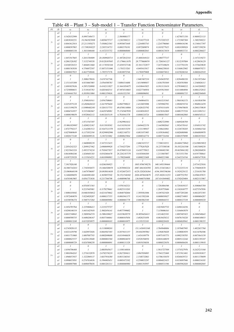
Appendix
242
Table 48 – Plant 3 – Sub-model 1 – Transfer Function Denominator Parameters. P1 D u1 u2 u3 u4 u5 u6 u7 d1
y1
a5 1 1 0 1 0 0 1 1
a4 0.5420352999 8.0997348473 1 2.3869080177 1 1 1.4276071350 0.9009321133
a3 0.0838202251 19.3943925899 3.0050675717 1.2303588213 1.7316577218 1.7515205325 1.1733907369 1.1983509221
a2 0.0043612914 25.2111950271 7.4568623565 0.0950071648 1.2244885743 1.2245796060 0.0990416196 0.1346417397
a1 0.0000587865 15.7308369225 2.2305534753 0.0003576191 0.0972009874 0.1019277635 0.0010388924 0.0057199256
a0 0.0000005338 1.3031046440 0.1472555752 0.0000068000 0.0000082843 0.0001673819 0.0000855731 0.0002286027
y2
a5 1 1 1 1 1 1 0 1
a4 1.0451917605 3.2031584009 20.1809928713 11.4872832543 15.0081649321 6.1080777537 1 2.1473339271
a3 0.2863526382 7.3152749558 29.8328307695 15.1796611678 28.7770606974 11.7200341127 1.8132397804 1.4128656129
a2 0.0168520323 7.4044811660 42.1170592104 15.0295527146 22.5011722877 7.2475549629 1.5337793339 0.1576429838
a1 0.0001565830 4.5760072507 15.8073351046 1.1703213263 4.0495433917 0.9666258010 0.3160632902 0.0066979271
a0 0.0000027823 0.4637748046 1.1585537176 0.0030872546 0.1769979908 0.0306874812 0.0158200344 0.0002642918
y3
a5 0 1 1 0 1 1 1 1
a4 1 2.3086378016 2.6197167746 1 1.9467407210 1.9249428705 1.8284486520 2.2613972464
a3 2.1511435309 4.8310667085 2.0764588783 5.8084314488 1.6519098957 1.6363781849 1.3820765884 1.2340026311
a2 2.6993655636 4.2951520880 0.4342313827 31.9441054075 0.4100443925 0.3913131619 0.2783000212 0.1443269922
a1 0.7258880651 2.5138165763 0.0203402531 47.9974534683 0.0227740954 0.0197615693 0.0110084894 0.0061252832
a0 0.0344441703 0.3838913084 0.0001359016 4.6163321593 0.0000096091 0 0.0000091735 0.0002504049
y4
a5 0 1 1 0 1 1 1 1
a4 1 5.3598101911 2.8591708683 1 1.5949844551 1.6933235365 1.5803362173 1.1033836709
a3 0.2251875118 12.4926620123 2.2417079420 6.0947788633 1.4110055096 1.5059902781 1.0926074734 1.9948612470
a2 0.0115399278 13.8988482383 0.5201517755 48.6768134884 0.2426325792 0.3074331450 0.1709470658 0.2901370838
a1 0.0004741857 9.5351062667 0.0439748981 75.3745687858 0.0100503835 0.0158161869 0.0083757216 0.0113091511
a0 0.0000198659 0.9528042112 0.0012035139 6.7816941578 0.0000124724 0.0000015847 0.0001662860 0.0004545131
y5
a5 0 1 0 1 0 1 1 0
a4 1 1.8713547307 1 2.5629963412 1 1.6082723890 1.6469246769 1
a3 35.9861829997 2.4200232367 8.0115818562 0.4110356330 1.6494422176 2.1445802043 1.5824570143 1.0549331742
a2 2.8727792217 1.2142883512 22.9247121578 0.0336515259 1.1331198937 1.3306434961 0.1226738205 0.1036841544
a1 0.0270069649 0.1171852194 38.8299892996 0.0021348753 0.0831071985 0.1058364062 0.0026080906 0.0046809970
a0 0.0020173140 0.0026099516 3.2367233062 0.0000625864 0.0000542774 0.0007724304 0.0001979098 0.0001855032
y6
a5 0 1 1 0 1 1 1 1
a4 1 1.9408888239 2.5475515435 1 2.0667435717 7.7306510551 26.6684770842 12.6398839832
a3 2.2054242323 3.2699327462 2.6900699928 4.7344257284 1.7776267628 14.2375588546 50.1852163500 5.6815009258
a2 2.9235643324 2.4953574234 0.7930457057 16.8786855124 0.4307778915 8.9368405390 38.6659041382 0.2862004856
a1 0.8636984246 1.0248401303 0.0542064478 28.2262187579 0.0185694369 1.2133687887 7.8153551784 0.0197788641
a0 0.0387529528 0.1335654221 0.0010990883 5.1788204688 0.0000232408 0.0040521906 0.2445554744 0.0005477836
y7
a5 1 0 1 0 1 1 0 1
a4 7.3917026348 1 6.8246384925 1 1805.9596748276 948.3495199444 1 2.0734325016
a3 16.9987542031 1.7392956975 19.3684508878 6.2878992224 4987.4841820789 3052.2536534611 4.7122255119 6.7594093878
a2 23.8969649199 1.6479796097 20.0938014038 32.9526072471 6129.3282656364 4194.3895596366 9.1929229152 1.2516181780
a1 9.1460099059 0.6404981404 4.3658855502 50.3521540302 2020.4876010679 1525.4928131253 4.4087552783 0.0506197671
a0 0.6593463905 0.0561753656 0.2317566708 4.4008996768 136.8468743808 107.0143049482 0.3592429484 0.0023315967
y8
a5 0 1 0 1 0 1 1 1
a4 0 4.8703871565 1 1.9795342521 0 1.7283884398 0.7293039537 0.3090645789
a3 1 9.2235405981 0.3178278661 0.0925333203 1 1.2818755606 0.1362030777 0.0273547056
a2 3.9080105692 10.8683050812 0.0231679662 0.0048792004 1.3959563496 0.1097421928 0.0077285200 0.0012071585
a1 0.5872469870 5.8224828287 0.0000137355 0.0001841375 0.1413582106 0.0008050927 0.0002734883 0.0000684287
a0 0.0190596374 0.5087515264 0.0000009984 0.0000001778 0.0003862549 0.0000044551 0.0000127238 0.0000009220
y9
a5 1 1 1 0 0 1 1 0
a4 0.3054785764 2.3359906413 1.2335275727 1 0 3.0239267732 2.2490124256 0
a3 0.0290146519 3.4431425918 2.3802456141 0.4877599682 1 7.1158006163 5.3164043879 1
a2 0.0012740843 2.5009564719 0.1986109627 0.0319638579 16.9856424413 1.6514622181 1.0697407423 0.1004546643
a1 0.0000588735 0.4486206167 0.0037346661 0.0000167656 3.4826251058 0.0618429212 0.0476154220 0.0046348653
a0 0.0000013248 0.0152850975 0.0000000165 0.0000010975 0.1195352183 0.0000220420 0.0004628941 0.0001398355
y10
a5 1 0 1 0 1 1 1 1
a4 0.2745828135 1 0.1118098203 1 151.1456953548 3.7849948084 2.1979487995 1.4822657760
a3 0.0221439790 1.6428972026 0.0045847365 0.2075031157 29.8362997861 1.2384676028 1.2308065859 0.6134784506
a2 0.0011753068 1.6807687745 0.0002698688 0.0334946658 1.4454349779 0.0975105773 0.0982558705 0.0673643158
a1 0.0000625557 0.4229118048 0.0000001560 0.0000824670 0.0528394850 0.0016340659 0.0005112244 0.0031395107
a0 0.0000008729 0.0247006258 0.0000000091 0.0000131328 0.0019356836 0.0000525676 0.0000404456 0.0001139918
y11
a5 1 0 1 1 0 1 1 1
a4 3.0394706468 1 2.0805845617 1.3188140016 1 1.5831727509 3.1574527976 0.2425215160
a3 5.9801864243 1.2716332870 2.6792576219 0.2627269411 3.0847056885 2.7941272468 5.8715913401 0.0189393657
a2 1.4946073937 1.3222869137 1.6037916380 0.0031240341 2.1548732063 0.3706318470 0.9240439721 0.0011378699
a1 0.0996855891 0.2747634656 0.1994905451 0.0005475502 0.2590855297 0.0004023455 0.0156097946 0.0000334105
a0 0.0000887906 0.0080078656 0.0001283311 0.0000000980 0.0001393897 0.0000533396 0.0005962020 0.0000002805
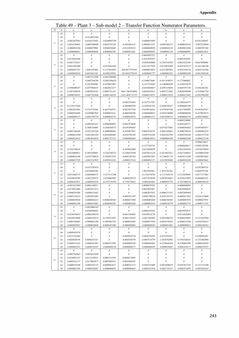
Appendix
243
Table 49 – Plant 3 – Sub-model 2 – Transfer Function Numerator Parameters. P1 N u1 u2 u3 u4 u5 u6 u7 d1
y1
b5 0 0 0 0 0 0 0 0
b4 0 -0.0114852360 0 0 0 0 0 0
b3 -0.0023079261 0.0164335978 -0.0200895799 0 -0.0004055095 0 0 0.0181282697
b2 0.0034330665 -0.0007400408 0.0032745330 -0.1003064131 0.0000055145 -0.0001909173 -0.0008010328 -0.0072229269
b1 -0.0000022186 0.0000079968 0.0000056640 -0.0121859332 -0.0000009959 -0.0000010139 -0.0000814506 -0.0005997186
b0 0.0000004643 -0.0000006004 0.0000003346 0.0000031483 0.0000000049 -0.0000001336 0.0000000099 -0.0000415031
y2
b5 0 0 0 0 0.0001807522 0 0 0
b4 0.0118910160 0 0 0 0.1033978507 0 0.0003384502 0
b3 0.0367370167 0 0 0 -0.0548384868 0.1505536789 0.0621832549 0.6615889000
b2 0.0041981086 0 -0.0578403402 0 -0.0112477858 -0.0724879498 -0.0367419712 -0.2421566706
b1 0.0000507331 1.9043147866 0.1133910438 -268.0677337434 -0.0000810825 -0.0153807854 -0.0072544176 -0.0635182366
b0 0.0000003630 0.0932461342 0.0388239502 -182.6822578418 -0.0000001757 -0.0000001261 -0.0000001948 -0.0011890148
y3
b5 0 -0.0013114288 -0.0012280469 0 0 0 0 0
b4 0 -0.0407344766 -0.2003386419 0 0.2348672648 0.2815438819 0.1773960062 0
b3 0 0.1027854980 0.2070622905 0 -0.1417372042 -0.1366884928 -0.1028141678 0
b2 0.5890488437 0.2877992619 0.0634013217 0 -0.0474004927 -0.0787310859 -0.0445187150 0.4362402392
b1 0.1027456076 -0.0092834763 0.0003721147 -4641.7907678691 -0.0030167615 -0.0052771691 -0.0028509980 -0.5250847724
b0 0.0000590585 -0.0047585806 0.0001144129 -2321.4891731725 -0.0000370251 -0.0000319270 -0.0000225462 -0.0567903099
y4
b5 0 0 0 0 0 0 0 0
b4 0 0 0 -0.9481559382 0.1527737729 0 0.1280244577 0
b3 0.1159177449 0 0 -0.2849407076 -0.1020343762 0.1648350547 -0.0846065740 0
b2 0.0022243464 0.3355772504 0.1051544571 -0.0253977703 -0.0199126161 -0.0738167036 -0.0157495007 0.4383647567
b1 0.0000564409 -0.0389667947 0.0099810141 -0.0005948706 -0.0000000833 -0.0582736998 -0.0000006280 -0.4579870372
b0 0.0000008737 -0.0043783719 0.0000692159 -0.0000428554 -0.0000001511 -0.0039496135 -0.0000002129 -0.0692368603
y5
b5 0 0 0 0 0 0 0.0005210000 0
b4 0 -0.0994365257 0.0004990659 -0.0027974626 0 0 0.0495148577 0
b3 0 0.1868729469 -0.2500369572 -0.6397489267 0 0.0710277604 -0.0480584462 0.0497685957
b2 0.0881384448 -0.0221563544 0.1808098062 -0.1850037621 0.0685838279 -0.0642340841 -0.0006756610 -0.0480902252
b1 -0.0000810388 -0.0015063329 0.0010486460 -0.0103702393 -0.0587518169 -0.0021622788 -0.0003030340 -0.0024717538
b0 0.0000214652 -0.0001630454 0.0001727514 -0.0000000442 -0.0008656014 -0.0000069189 -0.0000062280 -0.0000231190
y6
b5 0 0 0 0 0 0 0 0.0004224611
b4 0 0 0 0 0.1177128734 0 0.0900648011 0.0995328700
b3 0.3222398244 0 0 -0.3058024990 -0.0310029078 0 -0.0413039318 -0.0336578910
b2 0.0510489911 0.1865504605 -0.1562780715 -0.1499519708 -0.0470255178 0.1633647422 -0.0257349915 -0.0390018704
b1 0.0000834190 -0.0107780654 0.1926911970 -0.0041383703 -0.0028027845 -0.1104021718 -0.0018712208 -0.0028855661
b0 0.0000027520 -0.0015547693 0.0495014336 -0.0000127414 0.0000001237 -0.0129850840 -0.0000016240 -0.0000659441
y7
b5 0 0 0 0 0 0 0 0
b4 0 -0.0233585654 0 0 0 0 0 0.0787489714
b3 0 0.0536869346 0 0 1.9852945801 1.3825742162 0 0.0902797164
b2 0.0553082773 -0.0044984571 -3.4375137306 0 -0.1738376749 -0.1717429734 5.5515058049 -0.0177177061
b1 0.0189839789 -0.0012705472 -3.0720065887 -6.0688182519 -0.0757639938 -0.0678536843 -0.0526347885 0.0000962323
b0 0.0000103471 -0.0000567210 -0.1973736792 -0.7376776812 -0.0002263665 -0.0002855750 -0.1917480314 -0.0000180310
y8
b5 -0.0031915945 0.0001144851 0 0 0.0000678504 0 -0.0000048991 0
b4 0.0178052469 -0.0029515215 0 0 0.0033807883 0 0.0034909828 0
b3 0.0096293268 0.0089411649 0 0 -0.0062837031 0.0068151145 -0.0052999489 0
b2 0.0005519233 -0.0032831042 0 -0.0001011497 -0.0001790236 -0.0101345745 -0.0002013563 -0.0101139640
b1 0.0000018920 -0.0000024212 0.0006209544 -0.0000471890 -0.0000085668 0.0000190508 -0.0000097876 0.0000027954
b0 0.0000001298 -0.0000105062 0.0000004228 -0.0000002420 -0.0000002434 -0.0000194770 -0.0000003732 -0.0000137105
y9
b5 0 -0.0019066345 0 0 0 0 0 0
b4 0 0.0160506820 0 0 0.0096258192 0 0.0059970572 0
b3 0.4256979415 -0.0002309334 0 -0.0011503691 -0.0149514719 0 -0.0114628089 0
b2 0.0418674900 -0.0004550253 0.5745911097 -0.0001716955 -0.0017204902 -0.0291000722 -0.0009102005 -0.1531010564
b1 0.0001544442 -0.0000041360 0.1003061724 -0.0000014942 -0.0000471916 -0.0019376101 -0.0000154180 -0.0193701613
b0 0.0000059923 -0.0000030648 0.0000167308 -0.0000000084 -0.0000000182 -0.0000013681 -0.0000000811 -0.0002240421
y10
b5 0 0 0 0 0 0 0 0
b4 0.0009385476 0 0 0 0 0 0 0
b3 0.0353316364 0 0 -0.0016918754 -0.0044324562 4.4121816527 0 0.2290544383
b2 0.0020826456 0.0096245123 0 -0.0001836556 -0.0007154779 -2.2816782801 0.5502544024 -0.1121062886
b1 0.0000151242 -0.0046567497 0.0003037978 -0.0000095520 -0.0000284203 -0.1539641039 -0.2700462580 -0.0069326925
b0 0.0000001925 -0.0000318107 -0.0000008120 -0.0000000171 -0.0000000439 -0.0000474691 -0.0002450115 -0.0000197075
y11
b5 0 0 0 0 0 0 0 0
b4 0.0907764945 -0.0030141848 0 0 0 0 0 0
b3 0.0104081107 0.0315345810 0.0005351950 0.0048233699 0 0 0 0
b2 0.0002632177 -0.0179642877 0.0007609547 -0.0025666591 0 0 0 0
b1 0.0000183248 -0.0003301155 0.0000041637 -0.0000247112 -0.0502191488 -0.0654406655 -0.0387873745 -0.1513733548
b0 0.0000001599 -0.0000592867 0.0000000859 -0.0000000645 -0.0004321930 -0.0023742147 -0.0001834978 -0.0025601818
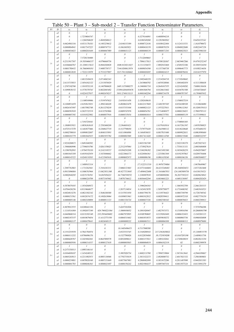
Appendix
244
Table 50 – Plant 3 – Sub-model 2 – Transfer Function Denominator Parameters. P1 D u1 u2 u3 u4 u5 u6 u7 d1
y1
a5 0 1 0 0 1 1 0 0
a4 0 1.7259684747 1 0 0.3279144091 0.4688894218 0 1
a3 1 1.1260394628 1.4849268612 1 0.0186549268 0.1283969563 1 8.6454335141
a2 0.0624803316 0.0531176183 0.1485259632 2.0340335389 0.0008712436 0.0108422404 0.1124333551 1.1610790672
a1 0.0000864841 0.0017547225 0.0000747711 0.1661605821 0.0000416539 0.0000870359 0.0046822606 0.0822447156
a0 0.0000054025 0.0000201649 0.0000067989 0.0000031125 0.0000000539 0.0000071293 0.0000025833 0.0025990330
y2
a5 0 1 0 0 1 0 0 0
a4 1 7.5728156988 1 0 3.7112049665 1 1 1
a3 0.2513917507 19.5850466537 4.8796669756 1 1.7896117013 4.0708320367 2.9659467266 19.0793252347
a2 0.0166660767 23.3288115612 8.0944369828 1698.9120211027 0.1311250472 1.9892932469 1.4549352186 10.5895524291
a1 0.0001780432 16.7660469181 5.9488759717 7144.0268613974 0.0009054390 0.1357568738 0.0996467773 0.9188214656
a0 0.0000014830 1.7222133878 0.7533237887 3215.5911026662 0.0000020205 0.0000024215 0.0000076016 0.0144357970
y3
a5 0 1 1 0 1 1 1 0
a4 1 1.6833249419 2.0714062343 0 2.2492446529 2.2534504718 2.1719249042 1
a3 2.6133735853 2.3054162122 1.2315876929 1 1.2419800792 1.4459528846 1.3093402459 4.3111380638
a2 1.2597102590 1.3919552118 0.1407800628 3405.3155088275 0.1900901710 0.2649167355 0.2214249292 7.8080130436
a1 0.1099838152 0.3576578743 0.0022065482 15389.6284493676 0.0091846794 0.0126633402 0.0104781508 2.8544726645
a0 0 0.0224327837 0.0002459237 5031.2740133113 0.0001042294 0.0000734378 0.0000787397 0.1769685932
y4
a5 0 1 1 1 1 0 1 0
a4 1 2.1308549906 1.5539747622 2.0192431458 2.1282038618 1 2.1506927219 1
a3 0.1200853459 2.6193615051 1.3892146228 0.4820623478 0.6612317669 2.1401587105 0.6524308528 5.3110624680
a2 0.0024347497 1.6837082748 0.2611270230 0.0337355304 0.0406821123 1.1973227011 0.0396112363 10.3268359313
a1 0.0000583918 0.2625732519 0.0132765866 0.0009747076 0.0000054761 0.1714696977 0.0000120451 2.7869795133
a0 0.0000007392 0.0101822982 0.0000857916 0.0000535654 0.0000003014 0.0066737581 0.0000005139 0.1571999631
y5
a5 0 1 0 0 0 0 1 0
a4 1 1.7193729101 1 1 0 1 1.7708805305 1
a3 1.1808955921 1.0856363618 2.7292406209 2.2364681621 1 1.6379165814 0.1637261397 1.6970780825
a2 0.0725317278 0.1403677466 0.2268627719 0.3127798050 1.7379775428 0.1643908112 0.0136220648 0.1974406352
a1 0.0002708010 0.0090832007 0.0040335893 0.0114904886 0.1464856031 0.0037835406 0.0009922651 0.0063898460
a0 0.0000165779 0.0003042935 0.0001955784 0.0000001968 0.0017413420 0.0000114768 0.0000155046 0.0000522597
y6
a5 1 1 0 0 1 0 1 1
a4 3.9216268673 1.8481040582 1 1 2.6031563748 0 2.5023336579 2.4872027412
a3 1.5966060996 2.7596054786 3.0261358025 2.2512197064 2.1738927610 1 1.7550131331 2.0885680008
a2 0.1580762893 1.8704570330 6.2143318557 0.8384293208 0.5160396382 2.6415495300 0.3650426259 0.4942870607
a1 0.0001645189 0.4939342959 3.5455696662 0.0223064373 0.0226904361 1.2255865369 0.0192397863 0.0289756406
a0 0.0000145525 0.0240110503 0.4153945616 0.0000682973 0.0000006196 0.0861439240 0.0000166336 0.0005846857
y7
a5 0 1 0 0 1 1 0 1
a4 1 1.3488935314 1 1 17.3122511519 11.9976759084 1 1.9678649967
a3 1.2997763883 1.1733262941 5.1916183331 5.9068121903 41.8751444681 26.6235248465 49.1040920453 2.8573263468
a2 0.8915096884 0.3006765964 13.0625851308 40.9277553695 17.4890422688 11.5416867951 124.1685889750 0.4330159321
a1 0.0902840295 0.0235156591 9.6365956223 64.7360749552 1.2180997818 0.8508099286 56.2837393233 0.0028619843
a0 0 0.0006524709 0.8875345902 5.0876736612 0.0036442294 0.0034601223 4.0483156997 0.0004282429
y8
a5 1 1 0 0 1 0 1 1
a4 0.5878079185 1.1854260972 0 1 1.1996204165 1 1.3065952789 2.2661203315
a3 0.0704426256 0.8319660677 1 1.2837134834 0.1424915878 1.5058758877 0.1710408392 2.0483910523
a2 0.0024833276 0.0823302142 1.5646100368 0.5337851950 0.0043799176 0.1339736421 0.0065749799 0.1726748542
a1 0.0000153561 0.0032674172 0.1492619064 0.0309051963 0.0001912812 0.0028599411 0.0003072318 0.0027759150
a0 0.0000005146 0.0002249889 0.0000811123 0.0001526724 0.0000037326 0.0002508342 0.0000076023 0.0002299913
y9
a5 1 1 0 1 0 0 0 1
a4 6.9678913555 0.6308441336 1 5.4247181826 1 1 1 5.7274766296
a3 1.1110514369 0.1892057190 429.7969223364 1.3000930052 0.1891926947 1.4827973571 0.1530954394 10.2868093798
a2 0.0449668314 0.0132182148 232.2954426682 0.0667972895 0.0108780605 0.2129262449 0.0066323423 2.1245201115
a1 0.0002187157 0.0010679454 11.4112771550 0.0004533462 0.0001853873 0.0059830272 0.0000865736 0.0966926808
a0 0.0000062137 0.0000478641 0.0024048135 0.0000008222 0.0000003511 0.0000060309 0.0000006513 0.0008979680
y10
a5 0 0 0 1 1 0 0 0
a4 1 1 0 10.1405496473 0.7117908588 1 0 1
a3 0.1553255978 0.7841784974 0 2.0525553745 0.1549288932 217.2563658822 1 15.1369873778
a2 0.0060111252 0.8766096176 1 0.1527780926 0.0122859480 38.1725859208 43.8167285190 2.4489831736
a1 0.0000428767 0.1025802201 0.0647889578 0.0052089611 0.0003157011 1.3085218261 4.1749030819 0.0822613150
a0 0.0000005956 0.0006514557 0.0000127418 0.0000005845 0.0000004819 0.0004162519 02 0.0002399978
y11
a5 1 1 0 0 0 0 0 0
a4 0.2373350513 1.0985346141 0 1 1 1 1 1
a3 0.0164699107 1.1454248512 1 5.3887026754 1.6002133768 1.7890719964 1.5671613641 4.2944189667
a2 0.0005203813 0.2211082973 0.0885136946 0.7792755619 2.3833322273 2.4826808752 2.4017021532 7.2901869601
a1 0.0000259881 0.0078820348 0.0007153449 0.0077667983 0.2868002099 0.3651672206 0.2811487098 0.9442051583
a0 0.0000001783 0.0006046363 0.0000023497 0.0000156242 0.0021904437 0.0097407334 0.0011857124 0.0133891270

Appendix
245
Table 51 – Plant 3 – Sub-model 3 – Transfer Function Numerator Parameters. P1 N u1 u2 u3 u4 u5 u6 u7 d1
y1
b5 0 0 -0.0007834414 0 0 0 0 0
b4 -0.0338356492 0 -0.0315665952 0 -0.0000021439 -0.0000192419 0 0.0045153607
b3 0.0301776976 0 -0.0053121674 0 0.0040476663 0.0032452578 0.0010091304 -0.0016282240
b2 0.0140949862 0 0.0006274727 0 -0.0022995834 -0.0013931431 -0.0007928835 -0.0009795173
b1 0.0002560498 0.1059939085 -0.0000548763 2.1151558888 -0.0006188477 -0.0005838876 -0.0008388003 -0.0000011262
b0 0.0000008188 -0.0004768229 0.0000103432 0.3311729829 -0.0000224284 -0.0000080936 -0.0000005116 -0.0000005073
y2
b5 -0.0184846410 0 -0.0002944467 0 0 0 0 0
b4 0.0810384065 0 -0.0219186891 0 0.0009506876 0.0006431024 0 0
b3 0.0088632961 -0.0091839383 0.0220363425 0.0004264313 0.1142628429 0.0904472615 0.0466980902 74.8080846124
b2 0.0008055759 0.0628592683 0.0210985004 0.0642341737 -0.0347750970 -0.0214851714 -0.0136025204 -11.8632378735
b1 0.0000014403 0.1265192953 0.0006871098 0.0220243148 -0.0354048641 -0.0283541830 -0.0180585215 -27.3714615130
b0 0.0000000894 0.0072920013 0.0000019087 0.0004261021 -0.0028003152 -0.0024734394 -0.0016085733 -2.7552698413
y3
b5 0 0 -0.0038665483 0 0 0 0 0
b4 0 0 -0.2351553374 0.0000653202 0.3334750819 0.0023662572 0.0015624268 0.0039707882
b3 0 0 0.1036103206 0.4022769915 -0.0748973720 0.2503254657 0.1508118546 0.2069935964
b2 0.7610818160 0.0879853685 0.1651986422 0.0707971505 -0.1686508411 -0.0586246364 -0.0416713834 -0.0806495677
b1 0.0009873382 0.1332497450 0.0141241480 0.0016807930 -0.0155037590 -0.1187766192 -0.0791482395 -0.0860416179
b0 0.0000586507 -0.0192131380 0.0000099600 0.0000033189 -0.0000063465 -0.0088194219 -0.0059006502 -0.0047182138
y4
b5 0 0 0 0 0 0 0.0011738672 0
b4 0 0 -0.2670754044 0 0 0 0.0649046836 0.0985489683
b3 0 0 -0.0254540389 0 366.5466737365 0.3576309291 -0.0045028046 -0.0262994496
b2 0.4676111287 0.0567671619 0.1596314933 16.9692099343 128.2578911893 -0.1924386477 -0.0588573853 -0.0655091469
b1 0.0305870794 0.1077690557 0.0000037001 3.1760631184 -438.3503112003 -0.1741303201 -0.0024768821 -0.0004834947
b0 0.0000478667 -0.0207364407 0.0000486728 0.0075766919 -21.9426757804 -0.0065944953 -0.0000523056 -0.0001182751
y5
b5 0 0 0 0 0 0 0 0
b4 0 0 -0.0053917706 0.2905631499 0 0 0.0367873596 0
b3 0 0 -0.2973991307 0.1573012703 0 0.1276513480 0.0086615083 0
b2 0 0.0365243746 -0.0374266176 0.0171685033 0.1571108624 -0.1367863356 -0.0471219762 0.7919520356
b1 0.1315696810 0.0880926956 0.2232469978 0.0000930574 -0.1858893549 -0.0059733543 -0.0003102722 -0.8466611454
b0 0.0005817011 -0.0201821327 0.0003432590 0.0000097933 -0.0045550288 -0.0004777067 -0.0001379901 -0.0510918158
y6
b5 0 0.0000707234 0 0 0.0010990922 0.0007250703 0.0005175091 0
b4 0 -0.0021435431 -0.0806746116 0 0.1361960283 0.1043612171 0.0615058756 0
b3 0 0.0006377914 0.0353710261 0 -0.0373723520 -0.0243133637 -0.0170871854 0.0833111531
b2 0.0815953559 0.0289230789 0.0319658425 0 -0.0554827045 -0.0425548187 -0.0277869460 -0.0263668555
b1 0.1864655531 0.0573189313 0.0002866695 514.8636293363 -0.0035866558 -0.0031687589 -0.0017197081 -0.0351883223
b0 0.0115851820 -0.0072259817 0.0000802179 365.3251647928 -0.0000723344 -0.0000358835 -0.0000081742 -0.0021230027
y7
b5 0 0 0 0 0 0 0 0
b4 0 0 0 0.0004502139 0.0012719269 0.0007935494 0 0
b3 0.0500173719 0 0 0.0692417993 0.1612725505 0.1055173894 0 0.4069008106
b2 0.0045825393 0.0132484841 -2.7496224761 0.0144507119 0.0243388723 0.0185549211 0.3704492862 0.1748114023
b1 0.0000814015 0.0106539823 -2.0246407717 0.0000311329 -0.0154721412 -0.0133039617 0.0130572166 -0.0468989629
b0 0.0000003379 -0.0025413087 -0.1399467106 0.0000059129 -0.0010789953 -0.0011855497 -0.0242764892 -0.0033795972
y8
b5 -0.0061329133 0 0 0 0 0 0 0
b4 0.0674823406 0 0 -0.0002233522 0.1161332399 0.0722334552 0.0336153509 0.0226864396
b3 0.0909113303 0 0 0.0001473781 -0.1337467241 -0.0867857635 -0.0423134413 -0.0428496923
b2 0.0049449922 0 0.0029813265 -0.0000020191 -0.0055539412 -0.0002096741 -0.0002188660 -0.0001005361
b1 0.0000110758 0.0194225230 0.0000069287 0.0000003528 -0.0000686603 -0.0001883988 -0.0000794953 -0.0000720798
b0 0.0000005686 -0.0082295989 0.0000002450 -0.0000000022 -0.0000024656 -0.0000004229 -0.0000004637 -0.0000003046
y9
b5 0 0 -0.0000670460 0 0 0 0 0
b4 0.0428659356 -0.0011640654 -0.0016707917 0 0 0 0 0
b3 0.0044701796 0.0029307348 0.0020057569 0 0.0237937628 -0.0014162852 0.0087702761 -0.0058547035
b2 0.0001204638 0.0004043665 0.0006396034 0.0007659521 -0.0621915416 -0.0163681898 -0.0260241408 -0.0135911429
b1 0.0000099848 -0.0001087345 0.0000321955 0.0000411847 -0.0053259803 0.0000035590 -0.0022290695 -0.0025697199
b0 0.0000000338 -0.0000015105 0.0000000827 0.0000000495 -0.0000036601 -0.0000189281 -0.0000009189 -0.0001108412
y10
b5 0 0 -0.0001871928 0 0 0 0 -0.0002760305
b4 0 0 -0.0008754998 -0.0000424609 0 0 0 0.0344216368
b3 0.4770412366 0 0.0007616054 0.0001743711 0.0811476813 0.0472161638 0 -0.0192596998
b2 0.0427129458 0.0047917692 0.0005645629 0.0000067874 -0.0048425156 -0.0022512850 0.0771350424 -0.0019015794
b1 0.0010259441 -0.0021258065 0.0000509866 0.0000004324 -0.0232991587 -0.0195810535 -0.0363200351 -0.0000716104
b0 0.0000021075 -0.0002939552 0.0000000442 0.0000000062 -0.0013160002 -0.0011003716 -0.0035566393 -0.0000025134
y11
b5 -0.0074984476 0 -0.0000399708 0 0.0006513002 0 0.0004555181 0
b4 0.1196562177 0 -0.0078493606 0 0.0695097696 0 0.0251706822 0
b3 0.0059563206 0 0.0057130378 -0.0021894093 -0.0473057556 0.0391406608 -0.0180913643 -0.0142529372
b2 0.0002889589 0.0152611939 0.0009538667 0.0012671029 -0.0767660486 -0.1121803292 -0.0300844740 -0.0397909026
b1 0.0000007541 0.0005537411 0.0012427103 -0.0000023441 -0.0046033002 -0.0067681569 -0.0005399470 -0.0036641346
b0 0.0000000272 -0.0061921005 -0.0000001013 0.0000001215 -0.0000015056 -0.0000105181 -0.0000292672 -0.0001114199
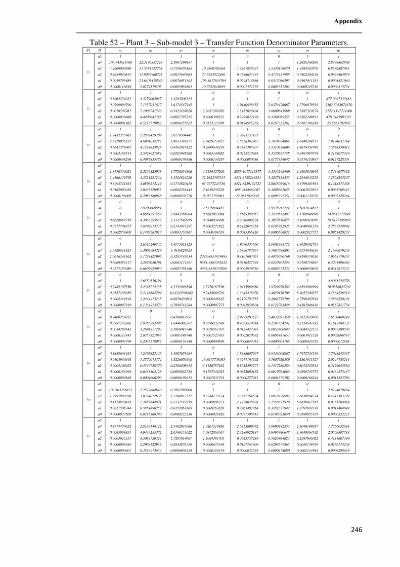
Appendix
246
Table 52 – Plant 3 – Sub-model 3 – Transfer Function Denominator Parameters. P1 D u1 u2 u3 u4 u5 u6 u7 d1
y1
a5 1 1 1 0 0 0 1 1
a4 10.0743618760 22.3195357228 2.3807299891 1 1 1 1.2426368266 2.8478862808
a3 3.2669003890 37.5581722754 0.7558476485 10.9508581644 1.4467858531 1.5330178970 1.9584587876 0.8586887061
a2 0.2654940855 51.8079960721 0.0827640983 73.7523822460 0.3538643391 0.4174437988 0.7402260218 0.0625464979
a1 0.0039795489 23.6105478840 0.0076051303 106.3817633764 0.0298714886 0.0315086395 0.0565011183 0.0004421940
a0 0.0000116848 2.0274519205 0.0005964805 10.7222616849 0.0007352679 0.0003637264 0.0000245216 0.0000314724
y2
a5 1 1 1 0 0 0 0 1
a4 0.3064254033 3.3279063067 1.4293206215 0 1 1 1 877.0097335184
a3 0.0299090799 7.1557031627 1.6174547945 1 1.9140948352 2.0376476667 1.7796079593 2302.5053671870
a2 0.0016507981 7.1003741540 0.3423169820 2.2021592050 1.5451026108 1.6809645969 1.5387310274 2122.1197711066
a1 0.0000036660 4.4406647366 0.0097797255 0.6000390521 0.2939022199 0.3369089355 0.3262248811 478.3482993331
a0 0.0000001985 0.5215519962 0.0000255622 0.0112123588 0.0138955259 0.0167325261 0.0167366249 25.5683792976
y3
a5 1 1 1 0 1 0 0 0
a4 1.2432355983 2.2878429309 2.0270504441 1 1.7883133121 1 1 1
a3 2.7229958523 4.6901035782 1.8833749371 1.9429153827 1.5628362967 1.7839304864 1.6949184537 1.9194037364
a2 0.5641778065 4.1244824828 0.4563927422 0.2849638219 0.3881395207 1.5310258606 1.4819354788 1.5884350013
a1 0.0003168514 2.5428021684 0.0265948288 0.0065140682 0.0225717884 0.3530697158 0.3491997474 0.3173077429
a0 0.0000638298 0.4085835373 0.0000193856 0.0000134297 0.0000080616 0.0175354047 0.0176110847 0.0127228591
y4
a5 1 1 1 1 1 1 1 1
a4 1.8176546621 2.5246325958 1.7728054806 4.2139327200 2888.1017115377 3.5316298469 1.4503840695 1.7439677312
a3 2.4166150798 4.5521251244 1.5524816256 42.2623597151 4331.3758213331 5.3257134355 1.2346945258 1.2868243207
a2 0.3995741933 4.0895213119 0.1753820414 65.7577245736 4421.8239154723 2.8045059616 0.1799405931 0.1418375468
a1 0.0162002038 2.0435529055 0.0004765443 7.1659258228 688.9334662087 0.3488662655 0.0063822833 0.0031768415
a0 0.0000158008 0.2082186948 0.0000536776 0.0171750961 22.9831825695 0.0095397551 0.0001130320 0.0002328264
y5
a5 0 1 0 1 0 1 1 0
a4 0 2.8209609881 1 2.5379894457 1 1.9535917224 1.5051624825 1
a3 1 4.6684291569 2.9443368004 0.5682052084 1.8589399057 2.3570512483 1.1708846096 14.9612715849
a2 0.8628689758 4.3036295632 2.3317549959 0.0346934996 2.2030809228 0.3057810875 0.1096919050 19.6177188069
a1 0.0717501875 1.8493013335 0.2143933291 0.0003273922 0.2432045354 0.0165932925 0.0040901254 2.7837558904
a0 0.0002858408 0.1493587927 0.0003350367 0.0000191659 0.0045366420 0.0006606032 0.0002827755 0.0951420273
y6
a5 0 1 1 0 1 1 1 0
a4 1 2.6525240745 1.9575012423 0 1.9076335660 2.0002483172 1.8629682761 1
a3 1.5120611823 5.3008584329 1.7936829623 1 1.6856787667 1.7683788805 1.6734046610 2.1690679258
a2 2.0616541162 5.1728427996 0.3285743034 2346.8953679495 0.4101603761 0.4476076169 0.4190578610 1.9663779107
a1 0.6069485517 3.2679630391 0.0065131391 9581.9363781622 0.0216427093 0.0250991244 0.0198776847 0.4731496483
a0 0.0277187089 0.6609924080 0.0007791340 4451.3530379269 0.0003959710 0.0002672234 0.0000930676 0.0212815222
y7
a5 0 1 0 0 0 0 0 1
a4 1 1.6550176194 1 1 1 1 1 4.6063138578
a3 0.2484307556 3.2348714335 4.3351093896 2.2970187596 1.9415969650 1.9529978584 4.6394969994 10.0356624239
a2 0.0157165059 2.3118883799 10.4245591662 0.2428666730 1.3642438970 1.4659156708 8.9055200257 8.5564226519
a1 0.0002446194 1.2444913235 6.6850430803 0.0009448162 0.2179783555 0.2664712796 4.7599487810 1.4836220101
a0 0.0000007919 0.1354913470 0.7099741284 0.0000997273 0.0085959504 0.0122783426 0.4365046410 0.0567851754
y8
a5 1 0 1 0 1 1 1 1
a4 0.7400256815 1 0.4380010397 1 2.9973293627 2.4032097350 1.9122620070 1.6508469249
a3 0.0997378266 2.9765392495 1.6446002301 0.0599332589 0.4053510814 0.2597754241 0.2124547192 0.1613104735
a2 0.0034288142 3.2691971293 0.1868047340 0.0029567707 0.0125427085 0.0052866947 0.0044522173 0.0035389580
a1 0.0000113145 2.0357321967 0.0005748348 0.0001525765 0.0002070692 0.0005487653 0.0003911328 0.0002696587
a0 0.0000003799 0.2036518082 0.0000156348 0.0000000899 0.0000044013 0.0000003166 0.0000016728 0.0000012668
y9
a5 1 1 1 0 1 1 1 1
a4 0.1838661485 1.2395827145 1.1087673084 1 1.8338607997 0.9436008867 1.7472743539 1.7043842367
a3 0.0105930448 1.3779075374 1.8226076098 16.3617758085 4.6971194602 1.7607926589 4.2801811327 2.0247788214
a2 0.0004103052 0.4540738570 0.2506308915 3.1126787162 0.8682593271 0.1417280586 0.8012335813 0.5126643830
a1 0.0000183994 0.0438305128 0.0089262734 0.1797342025 0.0322600152 0.0019764066 0.0296732771 0.0439373167
a0 0.0000000168 0.0004600290 0.0000192615 0.0001831791 0.0000277081 0.0001579702 0.0000166244 0.0011323786
y10
a5 1 1 1 0 0 0 0 1
a4 10.0303256873 2.2527884640 0.7882580906 1 1 1 1 2.8224679454
a3 1.9397990796 3.0374012638 1.7260037312 0.3784133174 3.3957164524 3.0819720997 2.6836894774 0.5743383799
a2 0.1124659418 2.3487844871 0.3131519759 0.0049896221 2.1726035878 2.2550391929 6.8856017745 0.0361704014
a1 0.0021508744 0.5854890757 0.0152863809 0.0009263826 0.2965492054 0.3182377942 1.3797697118 0.0013404049
a0 0.0000037509 0.0345366390 0.0000232236 0.0000026920 0.0097508915 0.0105023650 0.0599055159 0.0000322227
y11
a5 1 1 1 1 1 1 1 1
a4 0.1714470632 2.8163149122 2.4402934066 1.0261510926 2.6453699072 1.9090442353 2.1040198687 1.7556032618
a3 0.0085089835 4.9443255372 2.6590151022 5.0872864567 2.3284920247 3.9495940648 1.9640064592 2.0503307718
a2 0.0003015557 4.5024750324 1.7287019667 1.2064381705 0.3923757289 0.7626984824 0.2587946022 0.4111607399
a1 0.0000008950 2.2964122956 0.2043876559 0.0000675194 0.0151765909 0.0295677865 0.0056739749 0.0266174254
a0 0.0000000301 0.3523913633 0.0000001234 0.0000160119 0.0000042734 0.0000474080 0.0002143944 0.0006288629
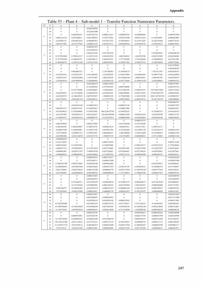
Appendix
247
Table 53 – Plant 4 – Sub-model 1 – Transfer Function Numerator Parameters. P1 N u1 u2 u3 u4 u5 u6 u7 d1
y1
b5 0 0 -0.0003398582 0 0 0 0 0
b4 0 0 -0.0128412996 0 0 0 0 0
b3 0 0.0026264473 -0.0037183714 0.0006134323 0.2000838754 0.2266069046 0 -0.0065871858
b2 0.0061243144 0.0831890611 0.0031908585 0.1497157262 -0.0927013696 -0.0854313423 0.1540238991 0.0000465880
b1 0.2244401151 0.0410823410 -0.0000067821 0.0774527353 -0.1905269933 -0.2119712587 -0.1016525640 0.0003774270
b0 0.0819371965 -0.0172775025 0.0000055159 0.0074412121 -0.0082899544 -0.0140656791 -0.1409328227 0.0000310042
y2
b5 0 0 -0.0003021472 0 0 0 0 0
b4 0 0 -0.0512095361 0 0 0 0 0
b3 0 0 0.2803122228 0.5417407438 0 0 2.4538636436 -0.0942408770
b2 25.7075822962 0.7998142125 0.1452219134 0.4910952854 1.0061286592 1.2620750798 -0.9043532802 0.0244584000
b1 55.7570703564 0.5160450721 0.3845366713 0.4607010355 -1.2777362802 -1.5163945644 -2.6360488410 0.0157011996
b0 11.9648468751 -0.1907211448 0.0576317456 0.0003823091 -0.4580917922 -0.5068752753 -0.3408726849 0.0007352902
y3
b5 0 0 0 0 0 0 0 0.0127278626
b4 0 0 0 0 0 0 0 -0.0428284385
b3 0 0.8034483315 0 2.7781586283 11.7045942151 0 1.7812271397 0.0025038550
b2 0.4162919516 0.3276532755 2.0151904942 3.5419922850 6.3441837096 6.9348203850 -0.3094577362 -0.0161289950
b1 7.6014871675 -0.4052022066 1.7057527905 2.8822344228 -22.6724407442 1.8900124851 -1.6807697765 -0.0034702875
b0 1.0729820159 -0.0479669569 0.5269880492 0.4324463116 -0.4187732684 -12.5499752187 -3.6163840643 -0.0000593525
y4
b5 0 0 -0.0014093235 -0.0000116922 0 0 0 0.0067977883
b4 0 0 -0.1165209181 0.7575281282 0.0007740098 0 0 -0.0025527132
b3 0 0.5351739296 0.3163992407 3.3189244621 0.1273603186 0.1280274375 330.7636535001 -0.0457772012
b2 2.6421893073 -0.1371362948 0.1646189750 4.6100959103 0.6845088906 0.8322515018 379.6819497745 -0.0005222381
b1 4.4165018718 -0.1306128933 0.0075591955 1.5666867430 -0.7769205868 -1.1016578108 -1029.7347565748 -0.0196991917
b0 0.9612782594 -0.0016481139 0.0001466214 0.1715775790 -0.6867056662 -0.4602403714 -76.3813793547 -0.0002068662
y5
b5 0 0 0 0 0 0 0 0.0063662791
b4 0 -0.0016245740 -0.1860813615 0 0.0000237138 0 0 -0.0346477925
b3 0.0053895371 0.0483617033 0.2140502433 0 0.2389612908 0 0 0.0040165453
b2 -0.8376299223 0.1526180904 0.1505437602 864.9228577558 -0.3497851651 0 -0.1792667512 -0.0103420215
b1 2.0313675005 -0.0978635515 0.0023302227 538.6023498569 -0.0000512058 -0.9029434218 -0.2581992596 -0.0003131471
b0 0.7146459775 -0.0032493318 0.0000080778 33.2321870313 -0.0000042460 -0.0124842603 -0.0456436148 -0.0000346203
y6
b5 0 0 0 0 0 -0.0000378755 0 0
b4 -0.0023199932 0 0.0001513809 0 -0.0147384266 0.1525516448 0 0
b3 0.3083462785 0.3604294067 0.1280724574 -0.0004423233 1.6638619913 1.6391517611 1.2095534113 0
b2 -0.0498637629 0.3249959981 0.1188537356 0.5079953789 -0.5572261664 -0.2339821176 -0.7101241574 -0.0008121933
b1 7.0275456640 -0.2098827211 0.1892933991 0.9604068347 -1.4067286888 -1.3697314009 -0.8339964915 -0.0000421838
b0 4.6456963606 -0.0361146598 0.0343235710 1.5900767538 -1.0237564982 -0.8606980441 -0.7551138863 -0.0000011240
y7
b5 -0.0090660443 0 0 0 0 0 0 0
b4 0.1361154939 0 0 0.0001145976 0 0 0 0.0007311580
b3 0.0022618497 0.1332832943 0 0.2100079488 0 0.3988102577 0.2078353239 2.1279349046
b2 0.0003617123 -0.0798180321 -4.1525012819 0.4952729480 0.6536951406 -0.2925474588 -0.1455037857 0.2462434441
b1 0.0000061067 -0.0029373397 -5.4899970700 0.8227220641 0.0720564407 -0.0527760191 -0.0108792681 0.0132675641
b0 0.0000000244 -0.0000698705 -0.4665294065 0.1110047450 -0.4805551391 -0.0004983488 -0.0000340141 0.0003645931
y8
b5 0 0 0.0000597834 0.0007357677 0 0 0 -0.0018952202
b4 0 0 0.0379109711 -0.0096537698 0 0 0 -0.0209951969
b3 17.9085383789 0.0502573669 -0.0281694100 0.0030610460 0 0 0.0550107877 0.0150684643
b2 14.2989020973 -0.0378907289 0.0190454649 -0.0003417507 2.4344135378 4.5893289523 -0.1856982552 0.0137340047
b1 0.0413756694 -0.0401359615 -0.0065323388 -0.0000026770 -6.8225717849 -11.9956767385 -0.0055775454 0.0014356325
b0 0.0353942091 -0.0003006556 -0.0001084591 -0.0000000649 -1.1151799933 -2.1266618392 -0.0000327975 0.0000295554
y9
b5 0 0 0.0000153605 0 0 0 0 -0.0016968762
b4 0 0 0.0433638547 0 0 0 0 -0.0523684977
b3 0 0.1216246751 -0.0315856378 -0.0208308522 -0.1258832777 -0.0004202275 -0.0155618198 0.0230860542
b2 0 -0.1731245054 0.0228995092 0.0061303242 -0.0471205992 1.4952302455 -0.0085044686 0.0251735267
b1 5.8587166577 -0.1040261685 -0.0107070135 -0.0006162257 -0.0040961430 -2.1842165275 -0.0007288477 0.0001947329
b0 1.2572294049 -0.0042478468 0.0000639651 -0.0000083170 -0.0000162427 -0.1852276197 -0.0000000692 0.0000114825
y10
b5 0 0 0.0001623035 0 0 0 0 -0.0018353810
b4 0 0 0.0673089495 -0.0000705401 0 0 0 -0.0511717960
b3 0 0 -0.0478286314 0.0364262148 -0.0006138581 0 0 0.0566271846
b2 67.3228702090 0 0.0354885129 -0.0568154112 4.8151792017 7.2711146122 -0.1444461821 0.0265605461
b1 65.1898780482 -0.3766336028 -0.0149266589 0.0251602309 -5.0707628558 -23.3401941305 -0.0943238049 0.0001725883
b0 6.1194779458 -0.0295829676 0.0000269414 -0.0002475046 -0.2711509269 -1.0229894540 -0.0080360579 0.0000098536
y11
b5 0 0 0.0000729156 0 0 -0.0001046413 0.0000790164 -0.0007400098
b4 0 0.0009572892 0.0335610378 0 0 0.0420177578 -0.0089247789 -0.0458348978
b3 34.7328738569 0.0360991818 -0.0204032260 -0.0123940750 0 0.0061682197 -0.0056313028 0.0217620767
b2 149.7146353288 -0.0217138523 0.0177874122 0.0036153116 -0.1061529931 -0.0998908739 -0.0004151771 0.0061949148
b1 211.9329117753 -0.0379328131 -0.0067663973 -0.0004301009 -0.0449717204 -0.1068282487 -0.0000038389 0.0059083117
b0 7.9725150141 -0.0016385502 0.0000512682 0.0000001888 -0.0024735329 -0.0071522208 -0.0000000153 0.0002043971
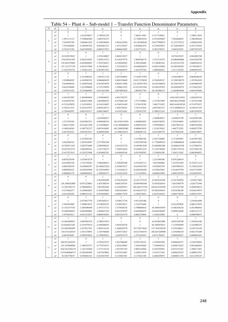
Appendix
248
Table 54 – Plant 4 – Sub-model 1 – Transfer Function Denominator Parameters. P1 D u1 u2 u3 u4 u5 u6 u7 d1
y1
a5 0 1 1 0 1 1 0 1
a4 1 1.4310356657 1.5300342720 0 7.5664111867 6.7517748643 1 1.1968113695
a3 1.5051111115 7.5700842960 1.0963742323 1 12.7208676101 12.0716958067 7.5024400032 3.3962490304
a2 7.4169785709 5.8684641201 0.1409186049 2.9016356768 44.1303902649 39.0577980873 12.1557370115 1.9926054656
a1 7.7931002049 4.1895987456 0.0018661321 1.1071529227 8.0526663279 8.1744919072 43.7226058855 0.1817518562
a0 0.7434371304 0.6012698262 0.0002357837 0.0906439202 0.2635752321 0.3622728472 5.6493230391 0.0072951879
y2
a5 1 0 1 1 0 0 1 1
a4 24.9192674822 1 1.4556148667 2.0640118257 1 1 9.6736345825 0.9444083596
a3 39.0330191398 4.5616318581 7.4292535253 8.5341879776 2.9848768579 2.7533134574 16.8866948666 4.6431892700
a2 170.4561979683 6.0458689893 5.7854794915 6.4780560205 8.7681958480 8.5748965244 61.6221913792 2.6698502243
a1 135.1313777736 4.4245277880 4.3381063811 3.7353562555 16.4440816855 14.8825350401 24.9285950267 0.2794188537
a0 11.6522745734 1.3548231433 0.4679873303 0.0030049472 1.9224797160 1.6806460932 1.8111710258 0.0089944397
y3
a5 0 1 1 1 1 0 1 1
a4 1 2.2235090102 1.5893511178 2.9477449893 17.3650717970 1 3.9764398975 0.6696306549
a3 1.9198606205 4.1445082185 9.8664684038 9.9602199460 29.8171970838 8.5546248222 13.5568590279 1.3957643639
a2 7.6364848442 2.5444676306 8.3635074670 8.9028131896 112.4565817953 16.8347496654 26.5294376475 0.4030660559
a1 9.6414558468 1.2321880609 4.7155359059 5.1896611052 61.0371653104 52.6562397855 30.2499309752 0.1150427621
a0 1.0392233352 0.1216400926 0.8153013200 0.6679085620 1.0658437748 26.5303460717 11.4829845836 0.0019393849
y4
a5 1 1 1 1 0 0 1 1
a4 2.0451027987 2.3869909926 1.5595698955 3.0931794755 1 1 1540.5467235021 1.0504385254
a3 8.4148592758 2.0656313608 1.0638060472 8.2370461169 1.7717729840 1.3771657499 1692.8621395940 1.7257225360
a2 11.5553478853 1.1132392951 0.1914516807 6.5540534108 7.3734374784 7.0621753652 9842.6140330749 0.7519770527
a1 6.7932215235 0.1933147877 0.0078128713 1.8282749101 7.1975155934 4.8837683753 3173.3688805233 0.2381913576
a0 0.7569482897 0.0023103117 0.0001390057 0.1616522463 1.2763815793 0.7068522318 173.6876366201 0.0023958705
y5
a5 0 0 1 0 0 1 1 1
a4 1 1 1.6536260237 1 1 1.5200038855 1.0248247799 0.6105907366
a3 1.2717583562 0.8247667431 0.9099498559 561.6705535950 3.4260892405 6.6818758076 5.7851659695 0.4929077323
a2 7.6643313092 0.6116011208 0.1103990847 2116.3690068822 0.4909558345 7.8799568053 4.0837687143 0.0887919200
a1 4.5480104264 0.1007742127 0.0015616005 465.2998285062 0.0000610418 1.1516158362 1.0467712581 0.0040572789
a0 0.4417052223 0.0025655637 0.0000052608 21.5096342472 0.0000087122 0.0141489770 0.0778441036 0.0002478887
y6
a5 0 1 0 0 1 1 1 1
a4 1 2.4722993181 1 0 5.5310082166 4.2915726868 5.1174385867 0.5455877402
a3 4.8422964324 5.2838349997 2.5773991590 1 13.6855997346 11.7726089219 12.7690686626 0.4060343822
a2 10.7849311103 3.8287974090 2.2889499243 3.2412553170 35.0939815038 25.8040893288 32.0646416746 0.1127666741
a1 30.0232912374 2.0058289341 1.5437144273 7.3288534454 23.0308253221 17.2165748405 19.4851729110 0.0155963146
a0 13.0157871611 0.3185325008 0.2054692391 6.0368993544 8.0518188585 5.5549924748 7.3843111007 0.0003694925
y7
a5 1 1 0 0 0 1 1 0
a4 0.6876230199 1.6756014279 1 1 1 1.2351969108 0.8781266014 1
a3 0.0144901228 1.5191109203 7.5004446872 2.5382487046 4.4741645112 7.6073840964 7.2235453449 52.5914111217
a2 0.0016588350 0.6240684587 20.1860222632 6.5936670137 10.4438953587 4.9782043358 3.0632089524 15.5564218341
a1 0.0000284225 0.0198395409 22.2301944851 5.1310146112 24.6285626282 0.5104835662 0.1636455799 0.6417332982
a0 0.0000001178 0.0004464652 3.3288044173 0.5144525226 5.5131859016 0.0046414989 0.0005307659 0.0324638587
y8
a5 0 0 1 1 1 1 1 1
a4 1 1 2.2834285098 0.7361934238 23.2917737232 32.9978236388 0.5227568859 1.0198573960
a3 128.1096262889 0.8751229881 3.3655508539 0.6682385593 28.0097801648 35.8459226914 7.4915580779 1.6201772496
a2 13.5265784174 0.5984408253 1.9815801894 0.1293683913 180.2463157736 248.0431429582 1.2235727340 0.2400528614
a1 0.3135662275 0.1269642665 0.7018978009 0.0018210495 62.9416337527 95.4629104453 0.0316386306 0.0146339974
a0 0.0331020382 0.0009331525 0.0556494005 0.0000137470 4.4360274053 6.9432224419 0.0001739910 0.0002517855
y9
a5 0 1 1 1 1 0 0 1
a4 1 2.8774817779 1.9975628151 1.8196117710 4.9313265380 0 1 1.2301641696
a3 3.5201045868 3.7468674675 4.3108201672 3.2190756211 3.1124754464 1 0.6121829692 2.6663573679
a2 11.3523377538 2.1082986490 2.1957117712 1.7278428156 0.7998668610 38.2894970079 0.1961658126 0.1833966924
a1 25.0589286693 0.6859999002 1.0858653720 0.8101479707 0.0429804975 29.8038380497 0.0099224608 0.0025313115
a0 1.4576923813 0.0433312827 0.0680591883 0.0635245170 0.0001539894 1.4326232980 0 0.0000768671
y10
a5 1 1 1 0 0 1 1 1
a4 41.2042469847 2.4807062576 2.1980315679 1 0 45.8230933608 0.8453182590 1.1850543188
a3 63.8444072346 4.5163979514 4.1805006285 1.9839329158 1 46.1892874631 7.1370768490 2.1443668352
a2 315.6983962985 3.2473817181 2.4893141183 5.3268249579 78.5738755642 337.7444740749 4.3791286011 0.2301741438
a1 130.6710120510 1.5053378891 1.1305768600 2.2893753643 54.6137403074 186.6457409890 1.4793886529 0.0021791498
a0 8.0034594481 0.2062010642 0.1290836933 1.6365915579 2.3555441659 6.8531784035 0.0946428037 0.0000843941
y11
a5 1 0 1 1 1 1 1 1
a4 260.8351402455 1 2.5764525272 1.8237906488 0.9793158125 1.4720493588 0.6900284371 2.2385459695
a3 393.1079848084 1.3496743573 4.7770743975 3.2916129883 7.1836393602 7.7188944322 0.2690712825 2.8832684043
a2 1842.8222284170 1.1241107640 3.3773118116 1.9257851593 4.9083162804 6.3283392895 0.0253552301 1.2886171481
a1 1219.8069608713 0.4305083699 1.4473429964 0.9518143485 1.6308112659 2.9145371304 0.0002421833 0.2808015387
a0 56.5483776673 0.0704681441 0.2634815830 0.1329023561 0.1174621380 0.2686299870 0.0000011356 0.0112495218
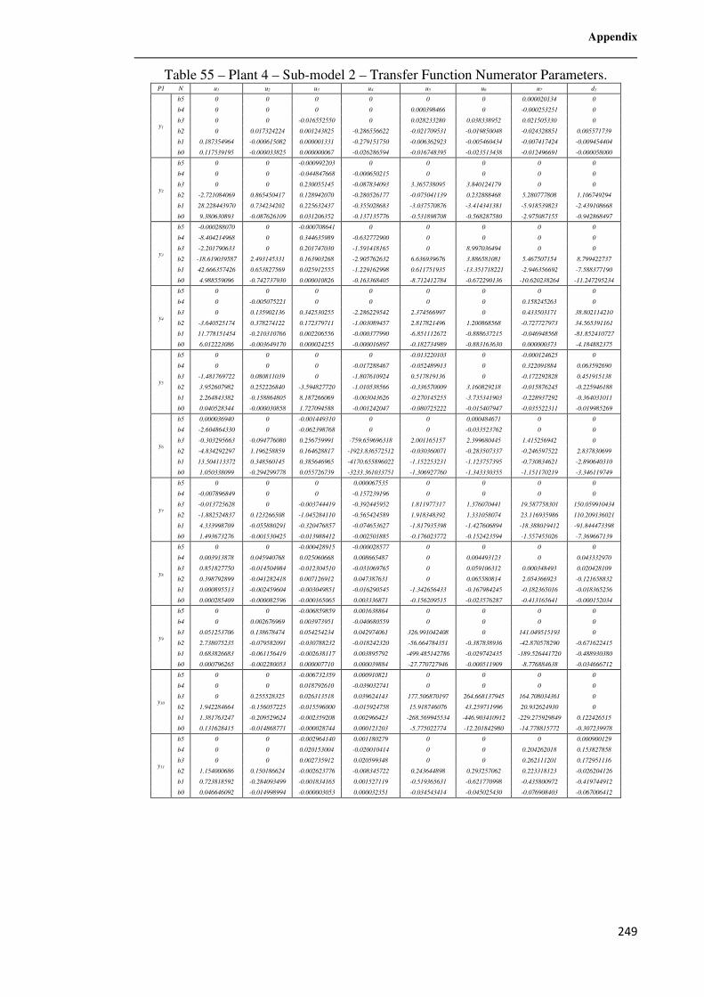
Appendix
249
Table 55 – Plant 4 – Sub-model 2 – Transfer Function Numerator Parameters. P1 N u1 u2 u3 u4 u5 u6 u7 d1
y1
b5 0 0 0 0 0 0 0.000020134 0
b4 0 0 0 0 0.000398466 0 -0.000253251 0
b3 0 0 -0.016552550 0 0.028233280 0.038338952 0.021505330 0
b2 0 0.017324224 0.001243825 -0.286556622 -0.021709531 -0.019850048 -0.024328851 0.005571739
b1 0.187354964 -0.000615082 0.000001331 -0.279151750 -0.006362923 -0.005460434 -0.007417424 -0.009454404
b0 0.117539195 -0.000033825 0.000000067 -0.026286594 -0.016748395 -0.023513438 -0.012496691 -0.000058000
y2
b5 0 0 -0.000992203 0 0 0 0 0
b4 0 0 -0.044847668 -0.000650215 0 0 0 0
b3 0 0 0.230055145 -0.087834093 3.365738095 3.840124179 0 0
b2 -2.721084069 0.865450417 0.128942070 -0.280526177 -0.075041139 0.232888468 5.280777808 1.106749294
b1 28.228443970 0.734234202 0.225632437 -0.355028683 -3.037570876 -3.414341381 -5.918539823 -2.439108668
b0 9.380630893 -0.087626109 0.031206352 -0.137135776 -0.531898708 -0.568287580 -2.975087155 -0.942868497
y3
b5 -0.000288070 0 -0.000708641 0 0 0 0 0
b4 -8.404214968 0 0.344635989 -0.632772900 0 0 0 0
b3 -2.201790633 0 0.201747030 -1.591418165 0 8.997036494 0 0
b2 -18.619039587 2.493145331 0.163903268 -2.905762632 6.636939676 3.886581081 5.467507154 8.799422737
b1 42.666357426 0.653827569 0.025912555 -1.229162998 0.611751935 -13.351718221 -2.946356692 -7.588377190
b0 4.988559096 -0.742737930 0.000010826 -0.163368405 -8.712412784 -0.672290136 -10.620238264 -11.247295234
y4
b5 0 0 0 0 0 0 0 0
b4 0 -0.005075221 0 0 0 0 0.158245263 0
b3 0 0.135902136 0.342530255 -2.286229542 2.374566997 0 0.433503171 38.802114210
b2 -3.640525174 0.378274122 0.172379711 -1.003089457 2.817821496 1.200868568 -0.727727973 34.565391161
b1 11.778151454 -0.210310766 0.002206556 -0.000377990 -6.851112672 -0.888637215 -0.046948568 -81.852410727
b0 6.012223086 -0.003649170 0.000024255 -0.000016897 -0.182734989 -0.883163630 0.000000373 -4.184882375
y5
b5 0 0 0 0 -0.013220103 0 -0.000124625 0
b4 0 0 0 -0.017288467 -0.052489913 0 0.322091884 0.063592690
b3 -1.481769722 0.080811039 0 -1.807610924 0.517819136 0 -0.172292828 0.451915138
b2 3.952607982 0.252226840 -3.594827720 -1.010538566 -0.336570009 3.160829218 -0.015876245 -0.225946188
b1 2.264843382 -0.158864805 8.187266069 -0.003043626 -0.270145255 -3.735341903 -0.228937292 -0.364031011
b0 0.040528344 -0.000030858 1.727094588 -0.001242047 -0.080725222 -0.015407947 -0.035522311 -0.019985269
y6
b5 0.000036940 0 -0.001449310 0 0 0.000484671 0 0
b4 -2.604864330 0 -0.062398768 0 0 -0.033523762 0 0
b3 -0.303295663 -0.094776080 0.256759991 -759.659696318 2.001165157 2.399680445 1.415256942 0
b2 -4.834292297 1.196258859 0.164628817 -1923.836572512 -0.030360071 -0.283507337 -0.246597522 2.837830699
b1 13.504113372 0.348560145 0.385646965 -4170.655896022 -1.152253231 -1.123757395 -0.730834621 -2.890640310
b0 1.050338099 -0.294299778 0.055726739 -3233.361033751 -1.306927760 -1.343330355 -1.151170219 -3.346119749
y7
b5 0 0 0 0.000067535 0 0 0 0
b4 -0.007896849 0 0 -0.157239196 0 0 0 0
b3 -0.013725628 0 -0.003744419 -0.392445952 1.811977317 1.376070441 19.587758301 150.059910434
b2 -1.882524837 0.123266508 -1.045284110 -0.565424589 1.918348392 1.331058074 23.116935986 110.209136021
b1 4.333998709 -0.055880291 -0.320476857 -0.074653627 -1.817935398 -1.427606894 -18.388019412 -91.844473398
b0 1.493673276 -0.001530425 -0.013988412 -0.002501885 -0.176023772 -0.152423594 -1.557455026 -7.369667139
y8
b5 0 0 -0.000428915 -0.000028577 0 0 0 0
b4 0.003913878 0.045940768 0.025060668 0.008665487 0 0.004493123 0 0.043332970
b3 0.851827750 -0.014504984 -0.012304510 -0.031069765 0 0.059106312 0.000348493 0.020428109
b2 0.398792899 -0.041282418 0.007126912 0.047387631 0 0.065580814 2.054366923 -0.121658832
b1 0.000895513 -0.002459604 -0.003049851 -0.016290545 -1.342656433 -0.167984245 -0.182365016 -0.018365256
b0 0.000285409 -0.000082596 -0.000165065 0.003336871 -0.156209515 -0.023576287 -0.413165641 -0.000152034
y9
b5 0 0 -0.006859859 0.001638864 0 0 0 0
b4 0 0.002676969 0.003973951 -0.040680559 0 0 0 0
b3 0.051253706 0.138678474 0.054254234 0.042974061 326.991042408 0 141.049515193 0
b2 2.738075235 -0.079582091 -0.030788232 -0.018242320 -56.664784351 -0.387838936 -42.870578290 -0.671622415
b1 0.683826683 -0.061156419 -0.002638117 0.003895792 -499.485142786 -0.029742435 -189.526441720 -0.488930380
b0 0.000796265 -0.002280053 0.000007710 0.000039884 -27.770727946 -0.000511909 -8.776884638 -0.034666712
y10
b5 0 0 -0.006732359 0.000910821 0 0 0 0
b4 0 0 0.018792610 -0.039032741 0 0 0 0
b3 0 0.255528325 0.026313518 0.039624143 177.506870197 264.668137945 164.708034361 0
b2 1.942284664 -0.156057225 -0.015596000 -0.015924758 15.918746076 43.259711996 20.932624930 0
b1 1.381763247 -0.209529624 -0.002359208 0.002966423 -268.569945534 -446.903410912 -229.275929849 0.122426515
b0 0.131628415 -0.014868771 -0.000028744 0.000121203 -5.775022774 -12.201842980 -14.778815772 -0.307239978
y11
b5 0 0 -0.002964140 0.001180279 0 0 0 0.000900129
b4 0 0 0.020153004 -0.020010414 0 0 0.204262018 0.153827858
b3 0 0 0.002735912 0.020599348 0 0 0.262111201 0.172951116
b2 1.154000686 0.150186624 -0.002623776 -0.008345722 0.243644898 0.293257062 0.223318123 -0.026204126
b1 0.723818592 -0.284093499 -0.001834165 0.001527119 -0.519365631 -0.621770998 -0.435800972 -0.419744912
b0 0.046646092 -0.014998994 -0.000003053 0.000032351 -0.034543414 -0.045025430 -0.076908403 -0.067006412
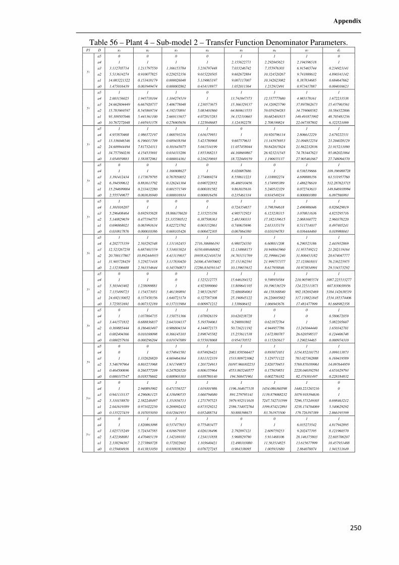
Appendix
250
Table 56 – Plant 4 – Sub-model 2 – Transfer Function Denominator Parameters. P1 D u1 u2 u3 u4 u5 u6 u7 d1
y1
a5 0 0 0 0 1 1 1 0
a4 1 1 1 1 2.155622771 2.292045623 2.194396518 1
a3 3.112705714 1.211797550 1.166153784 3.216797448 7.033246742 7.355976303 6.915465744 0.234923141
a2 5.513634274 0.910077825 0.229252356 9.015220505 9.602672884 10.324520267 9.741888632 4.890341142
a1 14.083221322 0.153418179 0.000026048 5.119065197 9.007117007 10.342623082 8.387834685 0.684647662
a0 1.475016439 0.003949474 0.000002862 0.414118977 1.052011364 1.212912491 0.973417887 0.004016623
y2
a5 1 1 1 0 1 1 1 1
a4 2.003156025 1.945718104 1.104274519 1 13.741847373 12.557777680 4.985178161 1.672233538
a3 24.662804449 6.667920737 5.406778048 1.230573675 15.366329137 14.320925790 37.897862673 15.437903561
a2 15.783969597 8.545869734 4.192370891 5.083401860 64.869613555 59.059294283 34.759068582 10.584322806
a1 93.309507046 5.441361100 2.669133657 4.072815283 34.152310665 30.682401815 149.491873992 48.705481256
a0 10.767272048 1.695931378 0.276905656 1.225848685 3.124382278 2.708199824 22.047387802 6.322521099
y3
a5 1 1 1 1 0 1 1 1
a4 4.955870468 1.986572197 1.068593216 1.616379951 1 10.920796114 2.806612229 2.679222531
a3 13.336046546 6.196011709 0.689438394 5.423780968 9.607579631 13.143976953 21.094812254 23.204028129
a2 24.609944494 7.817324311 0.301645075 5.041534199 11.057458044 50.842015624 21.862232836 21.915211090
a1 34.757560236 4.154535691 0.034333286 1.855368213 44.168669867 26.923231545 74.783447623 85.062021864
a0 3.054959883 1.583872961 0.000014361 0.216239693 18.722049159 1.190655137 27.905461667 27.748094370
y4
a5 0 0 1 0 1 0 1 1
a4 1 1 1.166908627 1 8.020087686 1 0.536539666 109.396988728
a3 3.391412434 1.173679795 0.767850052 2.774069274 8.558611223 1.318882274 4.699888356 63.531957760
a2 6.394509612 0.883613792 0.126241304 0.690722852 36.400510456 5.174995389 1.486276610 512.287623715
a1 15.294699004 0.233412280 0.001571749 0.000181582 9.863035616 5.240532329 0.072743633 149.846918994
a0 2.555749677 0.003636940 0.000016934 0.000016456 0.235461334 0.934549234 0.000001080 6.097566993
y5
a5 1 0 0 0 1 1 1 1
a4 1.301016207 1 1 1 0.724354657 3.798394618 2.496986046 0.826629819
a3 5.296408464 0.692935628 18.866376620 2.315255356 4.905712923 6.123238315 3.070811636 4.825295716
a2 5.140829659 0.477194755 23.335580512 0.387508363 2.481300331 17.182339615 2.068160772 2.960376220
a1 0.696868021 0.065991634 8.022723762 0.003152861 0.740635696 2.653335174 0.511714037 0.497405241
a0 0.010817876 0.000010386 0.668105426 0.000472305 0.067064380 0.010194783 0.036444460 0.018980043
y6
a5 1 1 1 1 1 1 1 1
a4 4.202775359 2.503292548 1.131162455 2716.306866191 6.980724350 6.608011208 6.290525186 2.443932869
a3 12.523267258 6.687401559 5.534033024 6350.688468002 12.134868173 10.948043960 11.955749212 21.202119164
a2 20.700137867 10.892444935 4.413139037 16938.621416734 34.765151769 32.399661240 31.800453182 20.674047777
a1 31.905728429 5.229271418 3.117830420 24306.474970682 27.151362591 21.999757377 27.123803031 76.236225975
a0 2.132306688 2.563354644 0.345760873 12286.834591147 10.139655632 8.617958846 10.973854991 29.534373292
y7
a5 0 0 0 1 1 1 1 1
a4 1 1 0 1.525212775 15.646184152 9.598950584 210.905985574 1087.225533277
a3 5.303443402 1.238099881 1 4.925099060 13.809641105 10.396536529 124.225111871 607.830038956
a2 7.135499723 1.154373051 3.461369891 2.983126397 72.686084063 44.158168840 992.182692469 5184.142638539
a1 24.692130052 0.337458356 1.640723174 0.327587308 25.190845122 16.220695882 317.118821845 1534.185374406
a0 3.725851691 0.007332189 0.137333984 0.009971212 1.538606432 1.066943676 17.481477999 81.668982358
y8
a5 0 1 1 1 1 0 0 1
a4 1 1.037804735 1.150751366 1.078926319 10.620238728 1 0 0.580672059
a3 3.441571832 0.688836837 2.643104137 5.393704063 9.298893802 0.621872764 1 5.082205607
a2 0.369885444 0.186403497 0.986804334 4.144072173 50.716211192 4.944957786 13.245044440 1.650342701
a1 0.002404366 0.010100098 0.366145103 2.898745582 15.255611538 1.672380787 26.620598537 0.124406748
a0 0.000257916 0.000296204 0.019747089 0.555018068 0.954170552 0.115265617 3.290234465 0.000974310
y9
a5 0 0 1 1 1 1 1 1
a4 0 1 0.574841581 0.874926421 2081.858566417 0.893071051 1154.852101751 3.099113873
a3 1 1.332626820 4.669464364 3.811312319 1533.809723062 5.129771122 783.027362888 6.169419589
a2 5.546797964 0.803273968 1.911749873 1.201724913 10397.960302253 2.820770453 5769.870189961 14.097644959
a1 0.464500696 0.266577209 0.247826520 0.806155964 4553.865240577 0.175659851 2228.040392591 4.651629793
a0 0.000337547 0.018576602 0.008903303 0.038780140 194.568471961 0.002756182 82.374301497 0.228184832
y10
a5 0 1 1 1 1 1 1 0
a4 1 2.940893902 0.471556527 1.019301986 1196.164677118 1454.086360598 1440.221265216 0
a3 0.941133137 4.296061125 4.318490735 3.660794680 891.279795141 1139.879068232 1079.918394636 1
a2 5.310158870 2.582248497 1.351856713 1.271797525 5979.952511618 7247.742733599 7296.571249305 0.698463212
a1 2.041619389 0.971022250 0.269092432 0.873529212 2586.734072764 3399.874212893 3258.174704069 5.540629292
a0 0.135227419 0.107055050 0.012041953 0.052488754 50.888398675 83.761975500 179.726397389 2.866195599
y11
a5 0 1 1 1 0 0 1 1
a4 1 1.820863098 0.537477653 0.775483477 1 1 6.035273542 4.817942895
a3 1.025735249 5.724347585 4.016679105 4.026136496 2.792897121 2.609759253 9.202477395 8.121960570
a2 5.422368081 4.470465139 1.142169181 1.234131858 5.968829790 5.911468106 28.146375803 22.605706207
a1 2.338294367 2.273860728 0.372022602 1.103640421 12.498103080 11.563514825 13.615677999 10.457931488
a0 0.159404936 0.413831050 0.030938263 0.076727245 0.984338095 1.005931680 2.864070074 1.941511649
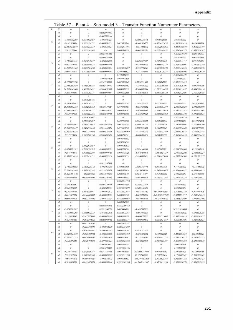
Appendix
251
Table 57 – Plant 4 – Sub-model 3 – Transfer Function Numerator Parameters. P1 N u1 u2 u3 u4 u5 u6 u7 d1
y1
b5 0 0 0.0003078410 0 0 0 0 0
b4 0 0 -0.0027553646 0 0 0 0 0
b3 -7.8813901300 0.0078812927 -0.0001749214 0 0.0596137512 0.0723026009 0.0606960333 0
b2 4.9541328914 0.0000624732 -0.0000086551 0.0218501740 -0.1062614552 -0.1204673414 -0.0809391419 0.0598309539
b1 12.3178130244 0.0000231634 -0.0000005514 -0.0002644975 -0.0554224031 -0.0322675066 -0.2136456849 -0.2964347494
b0 2.7433177944 0.0000001944 -04 0.0000548358 -0.0043030076 -0.0023148852 -0.0245464575 -0.0530336587
y2
b5 0 0 0.0025735342 0 0 0 -0.0001739439 0.0001820523
b4 0 0 0.0006428653 0 0 0 0.0161939753 0.0652812839
b3 -3.7259103435 0.2982538677 -0.0000044088 0 0.1452709981 0.3039379449 -0.0042641417 0.0959530254
b2 6.4027315976 0.2661949832 0.0000064794 0 -0.4146535925 -0.3886443174 -0.3247159901 -0.3406375149
b1 14.7385191563 0.0036803698 -0.0000000901 -0.0032970027 -0.7453754043 -0.9007970270 -0.5660436256 -0.6020060776
b0 2.9664130199 0.0001614490 0.0000000039 0.5969388827 -0.1812132559 -0.2226720378 -0.1273590702 -0.1374126410
y3
b5 0 0 0 0.2148379355 0 0 -0.0004022472 0
b4 0 0 -0.0002274839 0.0455407838 0 0 0.1397452217 0
b3 -7.2753955570 0 0.0567334501 0.0010508947 0.7260791905 1.3044547285 -0.0708552625 0
b2 22.5162003030 0.0415266836 0.0002489750 0.0002443561 -1.7792689222 -1.8991308802 -0.6947026796 0.8062354068
b1 24.7371142009 1.4667212491 0.0000831687 0.0000028039 -3.2460030814 -3.5168314433 -2.5361131097 -2.6345320116
b0 3.1066433413 0.0934791171 0.0000004437 0.0000002505 -0.4826128679 -0.5534360120 -0.3852472905 -2.1009419485
y4
b5 0 0 0 0 0 0 0 0
b4 0 0.0578205476 0 0 0 0 0 0
b3 -3.5374611605 0.3958542231 0 1.6057105067 1.0371295427 1.4716173222 0.6303762003 2.6292978387
b2 18.3850803360 0.0062010162 0.0779134627 0.2578369604 -2.0558604152 -2.0905761374 -2.1607916820 -2.9160987990
b1 15.5197100247 0.0034799171 -0.0001658711 0.0001858585 -3.9886381413 -3.9116724679 -4.0820321347 -8.0222565668
b0 3.7189101007 0.0000221356 0.0000204785 0.0005729095 -0.4358631948 -0.3866020962 -0.4915071372 -0.9101977831
y5
b5 0 0.0168763667 0 0 0 0 -0.0002019120 0
b4 0 0.7138329887 0 0.6297708807 0.0043678842 0.0049621034 0.2414631185 0.0127874532
b3 -2.3912330893 0.0896270025 0.0918977124 0.0016066214 0.1188198121 0.1576053729 0.1010573980 -0.1001860790
b2 19.1918862637 0.6424556650 0.0011669429 0.0119001517 0.2279822084 0.5063255249 -0.6900756684 0.8830177020
b1 12.8274346528 -0.0017544871 0.0000523001 -0.0001396960 -1.4187740071 -1.7790433460 -2.6598370573 -3.1916821448
b0 3.9573114461 0.0009800918 0.0000005973 0.0000213813 -0.0086490951 0.0388360880 -0.0951124650 -0.0492664494
y6
b5 0 0 0 0.0706733612 0 0 0 0
b4 0 0 0 0.0207584516 0 0 0 0
b3 0 1.1422873934 0 0.0003050577 0 0 0 0
b2 -3.6793826383 0.2089576785 -0.0000017571 0.0001239599 0.5884360208 2.9370625725 -0.1395774466 0.2533465661
b1 9.5841412199 0.1015553508 0.0000000923 0.0000007729 -2.7643235579 -7.1870654159 -1.7390703202 -2.6686161234
b0 12.8287734424 0.0002450712 -0.0000000059 0.0000001551 -2.9266581400 -1.5511477030 -1.2772386764 -1.1216775777
y7
b5 0 0 0 0 0 0 0 0
b4 0 0 0.0013207961 0 0 0 0 0
b3 -4.7369986868 1.5226125518 -5.4907178795 0.4342480658 1.5165193172 1.8952107035 1.1115668572 1.6515426592
b2 27.2943342986 0.3971392293 0.3539705973 0.0050559156 -1.6550793034 -1.5428689075 -1.6544466951 -1.8591646953
b1 19.8943984548 -1.0060839887 0.0037242815 0.0003102355 0.5430445077 0.3695229902 0.7206037151 0.1295402550
b0 4.1049546164 -0.0195030845 0.0005297982 0.0000013332 -2.9919447908 -4.0657177262 -2.1374718336 -2.7249294431
y8
b5 0 0 0 -0.0049913910 0 0 0 0
b4 -0.2700879067 0 0.0004720191 0.0003199634 0.0400323534 0 0.0342744355 0
b3 0.9082320035 0 -0.0001422605 -0.0000297072 0.0477446649 0 0.0204463981 0
b2 0.3162546063 0.1193010041 -0.0000592973 -0.0000021678 -0.0181810912 187.2644745804 -0.0063905770 0.2616489506
b1 0.0021617371 -0.1360649405 -0.0000002589 0.0000000069 -0.0839258531 -248.8398577541 -0.0527751717 -0.2986450039
b0 0.0002243505 -0.0053275442 -0.0000000134 -0.0000000037 -0.0180215969 -48.7561413701 -0.0158245099 -0.0421932408
y9
b5 0 0 0 0.0046545298 0 0 0 0
b4 0 0 0.0080896454 -0.0092309452 0 0 0 0
b3 -0.0796596767 0 0.0293368128 0.0014494796 -0.1097502565 0 28.0651836004 0
b2 -0.4691883298 4.0346612533 -0.0100402948 -0.0000972361 -0.0013398234 0 -15.6285868917 -0.6161125285
b1 3.1559813145 -4.3477479498 -0.0009828369 0.0000099379 -0.0000171260 -0.1523553064 -0.9176168419 -0.4609611627
b0 0.4521325467 -0.1872372600 0.0000000784 -0.0000003611 -0.0000001877 -0.0071834667 -0.0000681906 -0.0238351651
y10
b5 0 -0.0021910236 0 0.0022362523 0 0 0 0
b4 0 -0.3223348117 -0.0004705139 -0.0103374293 0 0 0 0
b3 0 0.8015688802 -1.4997430261 0.0007161044 0.4278241411 0 0 0
b2 14.0470914044 -0.1805404152 -0.3886000768 -0.0000591954 -0.5096854962 0.6933844728 -0.2132064054 0.8640926443
b1 17.2729521233 -0.6816666187 -1.3476226948 0.0000008382 -0.1182214281 -0.4783611514 -0.0850120317 -1.2478573533
b0 2.4406479625 -0.0508723970 -0.0371398115 -0.0000003245 -0.0490667508 -0.7888206341 -0.0036959423 -2.6133627232
y11
b5 0 0 -0.0015501843 0.0046944234 0 0 0.0001082916 0
b4 0 0 0.0001870485 -0.0086720126 0 0 0.1553330975 0
b3 0.2197181967 0.2921456187 0.0147135768 0.0013896454 193.3966314454 1.9846473991 0.3012837925 0.5720421718
b2 7.9222512861 0.0975208248 -0.0058357207 -0.0000953928 97.5252492772 0.7142287131 0.1755985547 -0.3680282601
b1 7.9048070491 -0.4004037227 -0.0002973473 0.0000083817 -284.2048200838 -3.1999825886 -0.4413844782 -0.9312461437
b0 0.5098634519 -0.0191079371 -0.0000017146 -0.0000002380 -44.7447313267 -0.4709133226 -0.0719020770 -0.0542867495
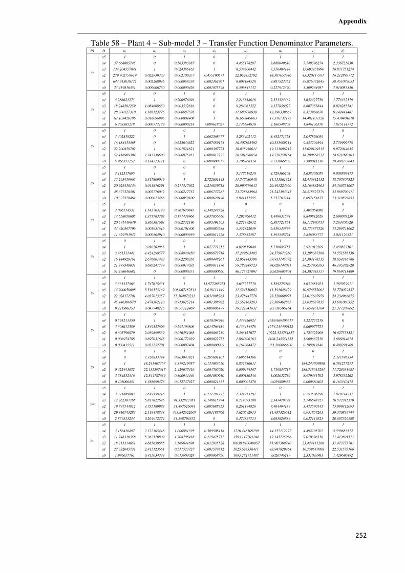
Appendix
252
Table 58 – Plant 4 – Sub-model 3 – Transfer Function Denominator Parameters. P1 D u1 u2 u3 u4 u5 u6 u7 d1
y1
a5 1 0 1 0 1 1 1 1
a4 37.668665745 0 0.563383387 0 4.455178287 3.688049610 7.749396274 2.336725830
a3 134.204557841 1 0.024366163 1 8.534806442 7.556484148 15.693451990 16.871751274
a2 279.702759619 0.022939333 0.002100357 0.455190671 22.952452702 18.387657446 43.320117501 16.212893712
a1 643.913018172 0.002268946 0.000068558 0.002362961 8.004184520 3.887523362 39.876372645 58.451079053
a0 73.419836351 0.000006760 0.000000426 0.001075598 0.506847132 0.227912390 3.509234987 7.010083536
y2
a5 1 0 1 0 1 1 1 1
a4 4.286621273 1 0.200976094 0 2.215338018 2.553324469 1.652427756 1.773432579
a3 18.248501259 1.084668650 0.003532616 0 9.284081522 9.557856027 8.607355844 8.926285541
a2 28.300127310 1.188123275 0.000687536 0 11.680736930 13.590339667 8.373988678 9.142441481
a1 62.103420186 0.016096996 0.000001408 1 16.663449663 17.336737175 14.481107520 15.439404610
a0 6.703565218 0.000717179 0.000000214 7.089618027 2.136584910 2.166548703 1.846136570 1.815114772
y3
a5 1 0 0 1 1 1 1 0
a4 3.402838222 0 1 0.062568677 3.283402112 3.482171523 2.047856039 1
a3 16.184455468 0 0.625646622 0.007389174 10.407865492 10.335989214 9.433209394 2.759999778
a2 22.200459702 1 0.001821821 0.000307773 18.038936011 19.113096212 11.029109315 9.972044635
a1 52.416909394 2.343336600 0.000875953 0.000013227 20.591696654 19.720259454 18.200658731 14.621090363
a0 5.966357252 0.114723121 0 0.000000357 3.706768374 3.711866802 3.389041116 18.488733643
y4
a5 1 0 0 0 1 1 1 1
a4 3.112517695 1 0 1 5.137619210 4.729366203 5.658405059 9.008899475
a3 15.293459965 0.317809049 1 2.722601143 11.747680948 11.155861328 12.436312132 18.707307325
a2 20.925458136 0.011876291 0.271517952 0.256859718 28.990779645 26.491224660 32.166832963 54.560751607
a1 48.377320501 0.002776032 0.000217752 0.006737287 23.728583964 21.242393345 26.518527379 53.889790971
a0 10.322528464 0.000013466 0.000059100 0.000629496 5.941111555 5.257763214 6.697151675 13.310593853
y5
a5 1 1 1 1 0 0 1 0
a4 3.096154531 1.543703170 0.967679843 0.348247728 1 1 3.405054086 1
a3 14.558056605 1.371783393 0.171439966 0.037056660 1.292766412 1.449631574 8.840812629 2.698078259
a2 20.691449649 0.360381693 0.002732196 0.005491505 6.272892912 6.387721851 18.117970711 7.264406920
a1 44.320367796 0.001931615 0.000101306 0.000083638 5.552822059 6.430535897 12.175877320 14.290741602
a0 11.329793932 0.000504910 0.000000959 0.000011228 1.378852587 1.591558724 2.836083777 3.041126321
y6
a5 0 1 0 1 1 1 1 1
a4 1 2.010202963 1 0.072771252 4.029819640 5.736085753 2.921012209 2.459827501
a3 3.461511441 4.424298577 0.008840450 0.006873718 17.249503405 24.579073280 13.208387368 14.551588136
a2 16.144929161 2.676601443 0.002208356 0.000448261 32.961443596 39.911145372 21.304178515 18.654346786
a1 21.479348031 0.695241749 0.000017033 0.000011176 59.784249723 94.028144081 38.257906583 46.145302920
a0 51.498646681 0 0.000000351 0.000000660 46.125727091 20.629605804 24.302745557 19.869711489
y7
a5 1 1 0 1 1 1 1 1
a4 3.361337463 1.747618431 1 13.972265975 3.655227730 3.589278046 3.633681923 3.585929911
a3 14.900058698 5.516573169 208.067182511 2.038111149 11.324550062 11.591648429 10.976552001 12.770029337
a2 22.028171701 4.037013357 55.504973213 0.031998263 23.478447776 23.526669971 23.015607979 24.234966675
a1 45.446306970 2.474302120 0.913625214 0.001388982 25.562163263 27.309462885 23.638587815 33.601060352
a0 9.221996153 0.047748225 0.057112469 0.000005479 19.122341631 20.710596164 17.654451564 21.317209892
y8
a5 1 0 0 1 1 1 1 0
a4 0.591213350 1 1 0.030394949 1.334456921 1659.969306617 1.223727258 0
a3 5.603612589 1.849337696 0.297193806 0.013766139 6.136414478 1274.231409122 6.069977721 1
a2 0.605796879 2.039899839 0.016581068 0.000063239 5.366157677 10222.324781857 4.723322908 16.627553321
a1 0.006974788 0.697031648 0.000172939 0.000022751 1.864606163 4108.245551552 1.900667250 5.688014674
a0 0.000415511 0.023252701 0.000002404 0.000000009 0.164084472 351.206066600 0.188019140 0.408291969
y9
a5 0 1 1 1 1 0 0 1
a4 0 7.326833344 0.803043921 0.265601101 1.696614366 0 1 2.311595354
a3 1 18.241407367 4.379219787 0.133083650 0.852736611 1 184.243709888 6.581257273
a2 0.422443672 22.135597617 2.429657416 0.004765020 0.009474567 1.710834717 188.718615281 11.723631983
a1 5.584832416 12.844787639 0.300944446 0.001080910 0.000136546 1.002052730 8.979331762 3.978532262
a0 0.405006451 1.388699473 0.012747927 0.000021351 0.000001470 0.039889655 0.000680401 0.163340474
y10
a5 1 1 0 1 1 0 1 1
a4 3.371889803 2.619358216 1 0.271291792 1.324955297 1 0.753506290 1.819314737
a3 12.262307765 5.817827676 94.332872781 0.148615774 6.714073100 2.343479393 5.746548727 16.572745570
a2 19.797144812 4.735189973 31.497626044 0.005688355 6.261194826 7.464494189 3.473570145 15.999312093
a1 29.816743283 2.118478838 443.842622607 0.001188766 1.620592913 11.937326612 0.951857263 59.570839744
a0 2.879553244 0.264912374 31.598793352 0 0.374857714 4.683826889 0.037119523 20.607526588
y11
a5 1 1 1 1 1 1 1 1
a4 3.156430497 2.322305418 1.000881395 0.509508418 1716.418109299 14.357112277 4.494295702 5.599683512
a3 11.748316358 5.262510809 4.708795418 0.215475737 1593.147203104 19.145725936 9.010398336 11.412691571
a2 18.215314651 4.683659685 3.569641698 0.012935528 10039.840046057 81.907369740 23.474111206 31.473773761
a1 27.332045731 2.415123661 0.511523727 0.001574812 5025.628356411 43.947829464 10.759617008 22.531573106
a0 1.976657761 0.415034344 0.015604028 0.000068750 1095.282711487 9.026746219 2.331043983 1.429690492

Appendix
253
Table 59 – Crude oil distillation – Plant 1 – Positive Uncertainty Parameters for the MVs. â6| y� y� yW yv y� y® y¯ y´ y¸ y�B y��
u� 0.6607 0.3192 0.2963 0.5641 0.4278 0 0.0587 0.0134 0.6541 0.7849 0.5214
u� 0 0.6799 0 0 0 0 0 0 0 0 0
uW 0.3342 0.2225 0 0.1849 0.2351 0 0 0 0 0 0
uv 0 0.2636 0.4556 0.4316 0.4755 0.5524 0.5927 0 0 0 0
u� 0 0 0 0 0 0 0 0 0 0 0
u® 0 0 0 0 0 0 0 0 0 0 0
u¯ 0 0 0 0 0 0 0 0 0 0 0
Table 60 – Crude oil distillation – Plant 1 – Negative Uncertainty Parameters for the MVs. â6. y� y� yW yv y� y® y¯ y´ y¸ y�B y��
u� 0 -0.2492 -0.4951 -0.4412 -0.5007 -0.4597 -0.5825 -0.844 -0.3716 0 -0.7136
u� 0 -0.7134 0 0 0 0 0 0 0 0 0
uW -0.3784 -0.2794 -0.3786 -0.1749 -0.1959 -0.2899 0 0 0 0 0
uv 0 -0.3154 -0.7255 -0.7252 -0.7771 -0.7661 -0.2611 0 0 0 0
u� 0 0 0 0 0 0 0 0 0 0 0
u® 0 0 0 0 0 0 0 0 0 0 0
u¯ 0 0 0 0 0 0 0 0 0 0 0
Table 61 – Crude oil distillation – Plant 1 – Positive Uncertainty Parameters for the DV.
��| w� w� wW wv w� w® w¯ w´ w¸ w�B w��
ë� 0 0 0 0 0 0 0 0 0 0 0
Table 62 – Crude oil distillation – Plant 1 – Negative Uncertainty Parameters for the DV.
��. w� w� wW wv w� w® w¯ w´ w¸ w�B w��
ë� 0 0 0 0 0 0 0 0 0 0 0