Embed Size (px)
Citation preview

©[2011]
Fei Song
ALL RIGHTS RESERVED

Chemical Characterization of Urban Air pollutants in Precipitation, Aerosols and Gas-
Phases in Northeast New Jersey in the US East Coast
by
Fei Song
A Dissertation submitted to the
Graduate School – Newark
Rutgers, The State University of New Jersey
in partial fulfillment of the requirements
for the degree of
Doctor of Philosophy
Graduate Program in
written under the direction of
Professor Yuan Gao
and approved by
____________________________
____________________________
____________________________
____________________________
Newark, New Jersey
May, 2011

ii
ABSTRACT OF THE DISSERTATION
Chemical Characterization of Urban Air pollutants in Precipitation, Aerosols and
Gas-Phases in Northeast New Jersey in the US East Coast
By Fei Song
Dissertation Director:
Dr. Yuan Gao
To chemically characterize urban air pollution in the US east coast, precipitation
for water-soluble inorganic/organic ions and trace metals, aerosols for trace metals, and
gas-phase samples for NOx, O3 and NO3 were studied in northeast New Jersey
metropolitan areas from 2006 to 2008. Precipitation and aerosols were collected by
automatic wet-only precipitation collector and MOUDI (Multi-Orifice Uniform Deposit
Impactor), respectively, while gaseous pollutants were measured by O3/NOx analyzers.
Results showed that sulfate (SO42-
) and ammonium (NH4
+) are the most dominant
ions controlling the precipitation acidity (pH 3.8 ~ 6.4). Acetate (CH3COO−) and formate
(HCOO−) are the major water-soluble organic acid species in the region. The elements Al,
Zn and Fe are dominant in the mass of the trace metals measured. Major sources for
pollutants in precipitation were identified as: (1) nitrogen-enriched soil, (2) secondary
pollution processes, (3) marine sources, (4) incineration, (5) oil combustion, and (6)
malonate-vanadium-enriched sources. About half of the precipitation events were
characterized by mixed sources.
For the size distributions of aerosol particles collected during this study, the total

iii
aerosol mass showed a typical bimodal distribution with two peaks around 0.32-0.56µm
and 3.2-5.6µm. Typical crustal trace metals (Fe, Cu, Mn and Sc) had coarse particulate
accumulation mode and their enrichment factors showed tilted normal distributions
pattern peaking at 1.0-1.8µm, while the other trace metals had fine particulate
accumulation mode and their enrichment factor showed monotonic decline patterns with
overwhelmingly high peaks in the size range of 0.18-0.32µm. Three major traffic related
sources for trace metals were identified: (1) brake wear and fuel combustion, (2) primary
fuel combustion, and (3) tire abrasion and fuel combustion.
Results from the gas-phase measurements showed significant diurnal and
weekday/weekend variations in the O3 concentrations, with higher concentrations being
found during the daytime and on weekends. The 24-h diurnal variations of O3 and NOx
showed a typical four-periods pattern: (1) morning NOx peak, (2) mid-day O3 formation,
(3) afternoon NOx accumulation, and (4) nighttime balancing. NOx and O3 showed
negative correlations indicating possible VOC-sensitive characteristics while no obvious
influence of HNO3 on O3 was observed.

iv
ACKNOWLEDGEMENTS
First and foremost, I would like to thank my advisor Dr. Yuan Gao for providing
me the opportunity to resume my PhD research and finally complete my PhD thesis at
Rutgers University. I will never find the words to thank her for all her contributions of
time, ideas, and mentoring and I much regret the fact that I will have little chance to pay
her back for all her personal dedications. With her enthusiasm, her inspirations and her
great effects to guide me to get everything planed and done in right way and in right time,
she helped me to qualify myself for a PhD candidate as much as possible. In every sense,
none of my PhD research work would have been possible without her. I am also thankful
for the excellent example she has provided as a devoted, loyal, persistent and successful
professional.
Many thanks must go to our department graduate director Dr. Alexander Gates
and department administrative assistant Ms. Liz Morrin. Dr. Gates has been always very
supportive whenever we need him. I could always learn something from him. Each time
after talking with him I would usually become more positive. I also appreciate his
dedication of his time and knowledge to my PhD research as one of my committee
members. Liz is the one who makes my life at Rutgers-Newark much easier and usually
the one who first comes to my mind when I need help. I would also like to thank her for
her trust and I would not forget the last conversation with her before I temporarily left
Rutgers-Newark in 2009.
It is an honor for me to also have Dr. Evert Jan Elzinga (Rutgers - Newark) and
Dr. Xiaoguang Meng (Stevens Institute of Technology) as my dissertation committee

v
members. Thanks for their professional comments and suggestions to improve my work. I
really appreciate the time they dedicated from their busy schedules. Their long-term
professional experiences, diverse knowledge and humble attitudes made them fantastic
committee members for my PhD research.
I would like to thank many people who have taught me the knowledge of
Chemistry, Environment Science, Instrumental Analysis, Biology, Geology, Statistics,
Programming et al., including Dr.Liping Wei and Dr. Joseph W. Bozzelli at NJIT, Dr.
Gary L. Taghon and Dr. Lisa Rodenburg at Rutgers-New Brunswick. I would also like to
thanks Dr. Andreas Vassiliou, a Rutgers-Newark emeritus professor, who has taught us
how to teach undergraduates geology labs.
I want to thank present and past members of our “Air Group” at Rutgers-Newark.
I thank Yunliang Zhao, Rafael Jusino-Atresino, Lili Xia, Lu Wang, Christopher Thuman
and Dawn Semple for the help with sampling, chemistry determinations, and discussions.
Without them, my research work would not be carried out so smoothly and efficiently. It
was such a good time staying together with them on the isolated coastal Rutgers Marine
Field Station in Tuckerton, NJ, on the roof of Bradley Hall on our campus, at the road
side of I95, and in the crowed Rutgers Marine Science ICPMS lab.
I am always very grateful that all faculties and graduate students in the Earth and
Environmental Science Department of Rutgers- Newark are so friendly and very helpful
all the time. With them, my PhD life has more joys and funs in both teaching and doing
research. I am especially grateful to Chi Zhang, Jincai Ma, Sweeta Chauhan, Mehrez
Elwaseif, Kisa Mwakanyamale and James Nolan. Special thanks go to Dr. Lee Slater, our

vi
new Graduate program director, who helped creat the department PhD handbook and
who is right there ready for any procedure questions.
I received a lot help from other institutions/departments for samplings and
chemistry analysis. Here I want to thank Dr. Jinyong Shin and Dr. Francisco Artigas from
the New Jersey Meadowlands Commission, Mr. Roland Hagan and Dr. Kenneth W. Able
from the Rutgers University Marine Field Station for their generous help for the aerosol
samplings. And Thanks to Mr. Paul Field from the Rutgers Inorganic Analytical
Laboratory and the technicians from NJIT Material Characterization Laboratories for
their great help in the ICPMS instrument determinations.
Lastly, my tones of thanks must go to my family. Thanks to my wonderful parents
Yuanfa Song and Zhuyu Shao who raised me and taught me with unreserved loves.
Thanks to my excellent sister Xiaofang Song for always supporting every decision I
made. Thanks to my wife Yi Xu for everything she did for me since we first met nine
years ago. It’s her who has companied me through every stop of my PhD journey. And
my loved son, Aiden Song, who brings me countless joys and happiness. I could not
describe how grateful I am to have him.

vii
Table of Contents
Chapter 1. Chemical Characteristics of Precipitation at Metropolitan �ewark in
the US East Coast........................................................................................... 1
1.1. Introduction .................................................................................................................. 4
1.2. Materials and Methods ................................................................................................ 6
1.2.1. Sampling............................................................................................................... 6
1.2.2. Chemical Analyses ............................................................................................... 6
1.2.3. Data Analysis ....................................................................................................... 7
1.3. Result and Discussion .................................................................................................. 8
1.3.1. Mass Concentrations ............................................................................................ 8
1.3.2. Acidity and Acid-Alkaline Equilibrium ............................................................. 11
1.3.3. Enrichment Factor Analysis ............................................................................... 13
1.3.4. Factor Analysis ................................................................................................... 14
1.3.5. Cluster analysis .................................................................................................. 16
1.4. Conclusions................................................................................................................ 18
1.5. References .................................................................................................................. 20
Chapter 2. Size Distributions of Trace Elements Associated with Ambient
Particular Matter in the Affinity of Highways in the �ew Jersey-�ew
York Metropolitan Area on the US East Coast ........................................ 44
2.1. Introduction ................................................................................................................ 47

viii
2.2. Methods ..................................................................................................................... 50
2.2.1. Sampling ............................................................................................................. 50
2.2.2. Chemical Determination ..................................................................................... 50
2.2.3. Data Processing .................................................................................................. 51
2.3. Results........................................................................................................................ 52
2.3.1. Concentrations and Seasonal Variations ............................................................ 52
2.3.2. Trace Metal Enrichment Factors ........................................................................ 53
2.4. Discussions ................................................................................................................ 54
2.4.1. Mass Size Distributions of Particulate Matter .................................................... 54
2.4.2. Mass Size Distributions of Trace Metals ............................................................ 56
2.4.3. Enrichment Factor Size Distributions of Trace Metals ...................................... 58
2.4.4. Trace Metal Sources Identification ..................................................................... 59
2.4.5. Weather Influence on Trace Metal Concentrations and Size Distributions ....... 62
2.5. Conclusions................................................................................................................ 63
2.6. References .................................................................................................................. 66
Chapter 3. Relationships among the Springtime Ground-level �Ox, O3 and �O3
in the Vicinity of Highways in the US East Coast ..................................... 87
3.1. Introduction ................................................................................................................ 89
3.2. Method ....................................................................................................................... 91
3.2.1. Sampling ............................................................................................................. 91
ix
3.2.2. Chemical determinations .................................................................................... 92
3.2.3. Data processing ................................................................................................... 93
3.3. Results and Discussions ............................................................................................. 93
3.3.1. Overall Concentrations and 24-hour Variations Characteristics ........................ 93
3.3.1.1. Concentrations ............................................................................................. 93
3.3.1.2. 24-hour Variations...................................................................................... 95
3.3.2. Weekday/Weekend and Diurnal Variation ....................................................... 96
3.3.3. Weather Influences on Concentrations ............................................................. 98
3.3.3.1. Daily Concentrations ................................................................................... 98
3.3.3.2. Diurnal Variations ....................................................................................... 99
3.3.4. Correlations between NOx and O3 .................................................................... 100
3.3.5. Correlations between NOx and OX ................................................................... 101
3.3.6. Relationships between NO3 and O3 .................................................................. 103
3.3.7. Multi-Regression analysis of the NOx-O3-NO3 system .................................... 103
3.4. Conclusions.............................................................................................................. 104
3.5. References ................................................................................................................ 107
Chapter 4. Conclusions ................................................................................................. 128
4.1. Conclusions of the three studies .............................................................................. 129
4.1.1. Pollution Sources .............................................................................................. 129
4.1.2. Temporal Variation Patterns ............................................................................. 130

x
4.1.3. Size Distribution Characteristics of Aerosol Mass and Associated Trace
Metals ............................................................................................................... 130
4.1.4. Others ................................................................................................................ 131
4.2. Recommendation for future research ....................................................................... 132
Appendices ..................................................................................................................... 134
I-1. Sampling information, precipitation amount and pH. .............................................. 136
I-2. Inorganic ions concentrations data (ppm) ................................................................ 138
I-3. Organic acids concentrations data (ppm) ................................................................. 140
I-4. Trace metals concentrations data (ppb) .................................................................... 142
II-1. Air concentrations (ng m-3
) of trace metals from the 1st set of winter intensive
sampling (12/11/2007-12/14/2007) ........................................................................ 145
II-2. Air concentrations (ng m-3
) of trace metals from the 2nd
set of winter intensive
sampling (12/14/2007-12/18/2007) ........................................................................ 145
II-3. Air concentrations (ng m-3
) of trace metals from the 3rd
set of winter intensive
sampling (12/18/2007-12/21/2007) ........................................................................ 146
II-4. Air concentrations (ng m-3) of trace metals from the 4th set of winter intensive
sampling (1/29/2008-2/1/2008) .............................................................................. 146
II-5. Air concentrations (ng m-3
) of trace metals from the 5th
set of winter intensive
sampling (2/21/2008-2/14/2008) ............................................................................ 147
II-6. Air concentrations (ng m-3
) of trace metals from the 6th
set of winter intensive
sampling (2/24/2008-2/27/2008) ............................................................................ 147

xi
II-7. Air concentrations (ng m-3
) of trace metals from the 1st set of summer intensive
sampling (7/3/2008-7/7/2008) ................................................................................ 148
II-8. Air concentrations (ng m-3
) of trace metals from the 2nd
set of summer intensive
sampling (7/7/2008-7/11/2008) .............................................................................. 148
II-9. Air concentrations (ng m-3
) of trace metals from the 3rd
set of summer intensive
sampling (7/11/2008-7/15/2008) ............................................................................ 149
II-10. Air concentrations (ng m-3
) of trace metals from the 4th
set of summer intensive
sampling (7/15/2008-7/19/2008) ............................................................................ 149
II-11. Air concentrations (ng m-3
) of trace metals from the 5th
set of summer intensive
sampling (7/19/2008-7/23/2008) ............................................................................ 150
III-1. NOx-O3 sampling weather data .............................................................................. 152
III-2. Ground level NOx-O3 concentration data (ppm) .................................................... 155

xii
List of Tables
Chapter 1
Table 1. 1 Summary of major anions, cations concentrations and pH in precipitation
(ppm). ................................................................................................................. 28
Table 1. 2 Summary of Trace Metals concentrations in precipitation (ppb). .................... 29
Table 1. 3 Concentrations of selected organic acids in precipitation at Newark (ppm). ... 30
Table 1. 4 Summary of Fractional Acidity and Neutralization factors of NH4+, Ca
2+ and
Mg2+
. .................................................................................................................. 31
Table 1. 5 Summary of Enrichment Factors. ..................................................................... 32
Table 1. 6 Varimax Rotated Factor Loadings ................................................................... 33
Table 1. 7 Scores of selected clusters model and seasonal distribution of precipitation
events .................................................................................................................. 34
Chapter 2
Table 2. 1 Summary of meteorological parameters during the sampling period. ............. 73
Table 2. 2 Summary of trace metal concentrations and the relative standard variations. . 74
Table 2. 3 Crustal enrichment factors of trace metals in fine, coarse and all particles. .... 75
Table 2. 4 Similarity levels of size distributions in/between different seasons (Centroid
Linkage Method). ............................................................................................. 76
Table 2. 5 Size distributions of trace metals by cluster analysis. ...................................... 77
Table 2. 6 Factor Analysis Result of trace metals concentrations ..................................... 78
Table 2. 7 Identified Clusters of MOUDI sampling events and their dominant factors. .. 79
Table 2. 8 Correlations between weather parameters and trace metal concentrations. ..... 80

xiii
Chapter 3
Table 3. 1 Ground level concentrations of NO, NO2, O3, HNO3 and NO3- .................... 113
Table 3. 2 Weekday/weekend and diurnal differences of NOx, O3 and NO3 ................... 114
Table 3. 3 Pearson correlations efficient among NOx, O3, NO3 and selected weather
parameters. ...................................................................................................... 115
Table 3. 4 Descriptive data of NOx, O3, NO3 under different weather conditions .......... 116
Table 3. 5 Rotated Factor Loadings for the factor analysis of NOx, NO3 and O3. ......... 117
Table 3. 6 Cluster analysis results with respect to NOx, NO3 and O3 .............................. 118

xiv
List of Figures
Chapter 1
Figure 1. 1 Map of sampling location ............................................................................... 35
Figure 1. 2 Electric charge equilibrium between total anions and total cations. ............... 36
Figure 1. 3 Pie charts of Annions, Cations, Trace Metals and Organic Acid, shown in
(a), (b), (c), (d) respectively ............................................................................ 37
Figure 1. 4 Dilution effect of Precipitation volume on total anions (a), total cations (b),
trace metals (c) and Organic Acid (d).. ........................................................... 38
Figure 1. 5 Histogram of pH. ............................................................................................ 39
Figure 1. 6 Correlations between major cations NH4+, Ca
2+ and major anions NO3
- and
SO42-
. ............................................................................................................... 40
Figure 1. 7 Correlations between Cl- and Na
+, K
+ in precipitation. .................................. 41
Figure 1. 8 Examples of the air mass back-trajectories for each cluster of the
precipitation with height of 20m, 500m and 2000m. ...................................... 42
Figure 1. 9 Examples of the wind speed and wind directions in precipitation periods. .... 43
Chapter 2
Figure 2. 1 Map of sampling location. .............................................................................. 81
Figure 2. 2 The mass size distribution of particles in winter and summer. ....................... 82
Figure 2. 3 The mass size distribution trace metals in two groups: (I) Coarse Particle
Accumulation and (II) Fine Particle Accumulation. ....................................... 83
Figure 2. 4 The mass size distributions of the 6 identified clusters of trace metals in
atmosphere (In the figure labels, W means winter while S means summer)...84
Figure 2. 5 The EF size distributions of the trace metal in three different clusters: (a)

xv
Cluster 1, (b) Cluster 2, (c) Cluster 3 and (d) Comparison of the average
patterns of the three clusters. ........................................................................... 85
Figure 2. 6 Back-Trajectories of air mass using NOAA HYSPLIT Model with arriving
height 5 m and duration 48 hours: (a). Cluster 1 (Sampling set #9 as
example), (b). Cluster 2 (Sampling set #4 as example), (c). Cluster 3
(Sampling set #5 as example), (d). Cluster 4 (Sampling set #6 as example).
For each sampling period (3- 4days), a total of 24 Back-Trajectories were
calculated with same interval (3-4 hours). ...................................................... 86
Chapter 3
Figure 3. 1 Study sampling site map ............................................................................... 119
Figure 3. 2 Box-whisker plot of daily averaged NO, NO2, NOx and O3 concentrations
in whole spring monitoring period. ............................................................... 120
Figure 3. 3 Time series of weekly averaged NOx, O3 and NO3 concentrations in spring
(Feb. 26th -May 20th
2007) ........................................................................... 121
Figure 3. 4 The 24-h temporal variations of hourly averaged NOx and O3. .................... 122
Figure 3. 5 The 24-h temporal variations of hourly averaged NOx and O3
concentrations in weekdays (a) and weekends (b). ....................................... 123
Figure 3. 6 The 24-h temporal variations of NOx and O3 in Clear days (a), Cloudy
days (b) and Rainy days (c). .......................................................................... 124
Figure 3. 7 Correlations between daytime averaged NOx and O3 in weekdays (a),
weekends (c), and between nighttime averaged NOx and O3 in weekdays
(b) and weekends (d). .................................................................................... 125
Figure 3. 8 Correlations between NOx and NO2/NOx ratio ............................................. 126

xvi
Figure 3. 9 Correlations between daytime averaged NOx and OX in weekdays (a),
weekends (c), and between nighttime averaged NOx and O3 in weekdays
(b) and weekends (d). .................................................................................... 127

1
Chapter 1 . Chemical Characteristics of Precipitation at
Metropolitan Newark in the US East Coast*
* This work has been published and could be referenced as “ Song, F., and Y. Gao, Chemical
characteristic of precipitation at metropolitan ewark in the US East Coast, Atmospheric
Environment, 43, 4903-4913, 2009 ”.

2
Abstract
To investigate the chemical characteristics of precipitation in the polluted coastal
atmosphere, a total of 46 samples were collected using a wet-only automatic precipitation
collector from September 2006 to October 2007 at metropolitan Newark, New Jersey in
the US East Coast. Samples were analyzed by ion chromatography for the concentrations
of major inorganic ions (Cl-, NO3
-, SO4
2-, F
-, NH4
+, Ca
2+, Mg
2+, Na
+, K
+) and organic acid
species (CH3COO−, HCOO
−, CH2(COO)2
2−, C2O4
2−). Selected trace metals (Sb, Pb, Al, V,
Fe, Cr, Co, Ni, Cu, Zn, Cd) in samples were determined by ICPMS. Mass concentration
results show that SO42-
is the most dominant anion accounting for 50.5% of the total
anions, controlling the acidity of the precipitation. NH4+
accounts for 48.6% of the total
cations, dominating the precipitation neutralization. CH3COO−
and HCOO− are the two
dominant water-soluble organic acid species, accounting for 42.0% and 40.2% of the total
organic acids analyzed respectively. Al, Zn and Fe are the three major trace metals in
precipitation, accounting for 33.6%, 26.8%, and 25.2% of the total metals. The pH values
in precipitation ranged from 3.8 to 6.4, indicating an acidic nature. Enrichment Factor
(EF) Analysis showed that Na+, Cl
-, Mg
2+ and K
+ in the precipitation are primarily of
marine origin, while most of the Fe, Co and Al are from crust sources. Pb, V, Cr, Ni are
moderately enriched with EFs ranging 43 - 414, while Zn, Sb, Cu, Cd and F- are highly
enriched with EFs > 700, indicating significant anthropogenic influences. Factor analysis
suggests 6 major sources contributing to the observed composition of precipitation at this
location: (1) nitrogen-enriched soil, (2) secondary pollution processes, (3) marine sources,
(4) incineration, (5) oil combustion, and (6) malonate-vanadium-enriched sources. To
further explore the source-precipitation event relationships and seasonality, cluster

3
analysis was performed and all precipitation events were grouped into 6 clusters. Results
show that about half of the precipitation events were characterized by mixed sources.
Significant influences of nitrogen-enriched soil and marine sources were associated with
precipitation events in spring and autumn, while secondary pollution processes,
incineration and oil combustion contributed greatly in summer.
Key Words: Precipitation, Trace Metals, Anions and Cations, Urban, Enrichment Factor,
Factor Analysis, Cluster Analysis.

4
1.1. Introduction
Precipitation plays important roles in carrying chemical species from the
atmosphere to the surface (Goncalves et al., 2000; Lara et al., 2001) and thus can bring
potential adverse effects to the terrestrial and marine aquatic ecosystems (Kim, 2000).
One of the consequent effects is “acid rain”, common in North America (Heuer et al.,
2000; Ito et al., 2002), which harmfully affects human health, damages buildings, and
acidifies aquatic systems. On the other hand, precipitation is episodic in nature and many
dissolved chemicals in precipitation can also serve as the sources of nutrients to enhance
biological activities and stimulate marine primary production (Pearls, 1985; Spanos et al.,
2002). Characterization of precipitation is critically important to better understand its
effects, develop control strategies and protect the environment.
The chemical characteristics of precipitation can be affected by many
environment impacts, including anthropogenic emissions (Lara et al., 2001), sea spray
and terrestrial dust (Safai et al., 2004; Das et al., 2005). In precipitation, the major
inorganic ions NO3- and SO4
2- can be transformed from their precursor gases, such as
SO2 and NOx emitted from pollution sources (Seinfeld and Pandis, 2006). NH4+ primarily
comes from fertilizers used in agriculture, biomass burning, livestock breeding and even
natural activities (Topcu et al., 2002; Hu et al., 2003; Migliavacca et al., 2005). Other
major elements Cl-, Mg
2+, K
+ and Na
+ originate mainly from natural sources such as sea
spray, rock and soil re-suspension and forest fires (Đorđević et al., 2005). Trace metals in
precipitation are strongly affected by anthropogenic pollution sources (Nriagu and
Pacyna, 1988), except Fe, Al and Mn which originate mainly from the earth's crust.
Organic acid species mainly come from direct anthropogenic emissions, biogenic

5
emission and in situ production from precursors in the troposphere. (G. Brooks et al.,
2006 and references therein)
The acidity of precipitation, a measure of active H+ concentration, is controlled by
the balance between acidification and neutralization processes. NO3- and SO4
2- are the
two major ions contributing to the acidity of precipitation (Zunckel et al., 2003;
Migliavacca et al., 2004). Organic acids, especially formate (HCOO−) and acetate
(CH3COO−), also contribute to the acidity of precipitation in both rural and urban areas
(Keene and Galloway, 1984; Yu et al., 1998; Pena et al., 2002). About 16-35% of the
total acidity was contributed by organic acids in North America (Keene et al., 1983). The
neutralization of the acidity is mainly caused by Ca2+
(Saxena et al., 1996; Basak and
Alagha, 2004) and NH4+ (Zunckel et al., 2003). With high rates of anthropogenic
emissions in the US East Coast, acid rain has been observed as a common feature in the
region. However, few studies on detailed precipitation chemistry have been conducted
recently in this region.
To characterize precipitation chemistry in this region, a one-year precipitation
sampling was carried out at Newark, New Jersey, with the following objectives: (1)
identifying the chemical characteristics of precipitation in this area; (2) investigating the
factors controlling the acidity of the precipitation; and (3) identifying the relative
contributions of different sources of chemical species in precipitation. The results of this
work will fill the data gap of precipitation chemistry for this geographic region and help
better understand the major processes and sources that control precipitation composition.
This study can also provide important insights into the linkages between urban air
pollution and its potential influence on human health and aquatic ecosystems.
6
1.2. Materials and Methods
1.2.1. Sampling
Event-based precipitation sampling was conducted in Newark (40º44′N, 74º10′W),
New Jersey in the US East Coast (Fig. 1.1) from September 2006 to October 2007.
Located on the US East Coast, Newark is the largest metropolitan center of the state,
adjacent to New York City and the Atlantic Ocean. The composition of precipitation in
this area could be influenced by both continental and marine sources. An automatic wet
only precipitation sampler (Type B1C, M.I.C Company, Canada) was set on the roof of a
building of ~ 20m height on the Rutgers University campus in downtown Newark for
sample collection. Before sampling, clean techniques for the sampler and bottles cleaning
were used, following the procedures by Kim et al., (2000). After each sampling, samples
were kept in a freezer until analysis. A total of 46 samples were collected during the study
period. The precipitation volume and other weather parameters for this sampling site
were obtained from a nearby weather station at Newark Museum
(www.wunderground.com).
1.2.2. Chemical Analyses
The major inorganic ions and organic acid species in the precipitation were
measured using ion chromatography (ICS-2000, Dionex) in the Atmosphere Chemistry
Lab of Rutgers University at Newark. The major inorganic ions include Cl-, NO3
-, SO4
2-,
F-, NH4
+, Ca
2+, Mg
2+, Na
+, K
+, and organic acid ions include Acetate, Formate, Malonate
(CH2(COO)22−
) and Oxalate (C2O42−
). Samples were first taken out from the freezer and
thawed overnight at room temperature, and then were filtered by PTFE syringe filter
(0.45 µm). Samples were injected into the IC system via automated sampler (AS40,

7
Dionex) using 0.5ml vials. An AS11 analytical column (2_250mm2, Dionex), KOH
eluent generator cartridge (EGC II KOH, Dionex) and 25µl sample loop were employed
for the determinations of anions, while for cations, a CS12A analytical column
(2_250mm2, Dionex), MSA generator cartridge (EGC II MSA, Dionex) and 25µl sample
loop were used. The detection limit of the method is below 0.01ppm, and the precision of
the analysis is ~ 1%. Detailed information of the method is given in Zhao and Gao (2008).
Strong linear correlations existed between the two electrically charged groups of anions
and cations with a slope of ~1.00 (R2 =0.875) (Fig. 1.2), suggesting that good electric
charge equilibrium existed between the two groups. Therefore the sampling and
determination methods in the study are reliable (Rastogi and Sarin, 2005).
Selected trace metals including Sb, Pb, Al, V, Fe, Cr, Co, Ni, Cu, Zn and Cd were
determined using High Resolution Inductively Coupled Plasma Mass Spectrometry (HR-
ICP-MS) (Finnigan™ ELEMENT2, Thermo Scientific) in the Institute of Marine and
Coastal Science at Rutgers University. Before determination, samples were filtered using
the same procedure as indicated above and then acidified to ~ 4% acidity by adding nitric
acid (Optima A460-500, Fisher Scientific). The detection limits for all trace metals are
less than 1ppt and the precision of the method is ~2%. More information on the ICPMS
methods can be found at http://marine.rutgers.edu/.
1.2.3. Data Analysis
Enrichment Factor Analysis, Factor Analysis and Cluster Analysis were employed
to explore the possible sources affecting the chemical characteristics of precipitation.
Enrichment Factor distinguishes the relative contributions of crustal or marine sources
from other sources (Chabas and Lefevre, 2000; Okay et al., 2002). Factor analysis was

8
used for further identifying the more detailed information of all possible major sources.
In this study, Factor Analysis was carried out using SAS 9.1 with principle components
analysis and Varimax Rotations. Based on the sources information from Enrichment
Factor Analysis and Factor Analysis, precipitation events were then grouped and
characterized separately by Cluster Analysis to explore the source-precipitation event
relationships and seasonality, using SAS 9.1 according to the Ward’s method (Ward,
1963). This method is appropriate for the quantitative variables, since it takes the Cluster
Analysis as a variance problem instead of using distance matrix or association measures.
After analysis, each cluster was realized in a multivariate distribution.
1.3. Result and Discussion
1.3.1. Mass Concentrations
Fig. 1.3a shows that SO42-
is the most predominant anion, accounting for 50.5%
of the total anion mass, followed by NO3- (24.6%), organic acid (13.8%), Cl
- (10.6%), and
F- (0.5%). The mass contribution of organic acid species to the total anions from this
study is similar to the results of Keene et al. (1983) for North America. For cations (Fig.
1.3b), NH4+ and Na
+ are the dominant contributors to the total cation mass, accounting
for 48.6% and 27.9% respectively, followed by Ca2+
(13.5%), K+ (5.50%) and Mg
2+
(4.50%). The high percentage of NH4+, which is mainly non-crust originated, indicates a
high anthropogenic contribution to the study area. This could also be confirmed by the
relatively low concentration of the crust-originated element calcium (Table 1.1). Besides,
the high mass percentage of Na+ may reflect the significant influence of marine sources.
For trace metals, the contributions of Al (33.6%), Zn (26.8%) and Fe (25.2%) are
overwhelmingly high compared with other trace metals (Fig. 1.3c), suggesting a mixed

9
influence of crust soil and anthropogenic emissions. Other trace metals including Cu, Pb,
Ni, Sb, and V contributed about 13.8% of the total trace metal mass, while the percentage
contributions of Cr and Cd were small. Similar to the observations in other regions
(Injuk and van Grieken, 1995; Herut et al., 2001; Hou et al., 2005), the abundance
sequence of Zn > Fe > Cu was also observed in the study. For organic acid species, the
VWA concentrations of acetate and formic acid are 0.21ppm and 0.20ppm, respectively
(Table 1.3), together contributing to 82.2% of the total organic anions (Fig. 1.3d), and this
result is consistent with the data from other urban regions (Keene and Galloway, 1984;
Yu et al., 1998; Pena et al., 2002). Oxalate and malonate are the additional organic acidic
species in precipitation observed in the area of this study.
Concentration dilution effects caused by high precipitation rate were observed for
total anions, total cations and total trace metals, but not for total organic acid. Fig. 1.4
shows that the concentrations of inorganic anions, major cations and total trace metals
decreased exponentially with increasing precipitation rates, while no obvious
relationships were found between total organic species and precipitation rates. This could
also be confirmed by the fact that event-averaged concentrations are higher than VWA
concentrations (Tables 1.1 & 1.2). The observed exponential relationships could be
attributed to the below-cloud raindrop scavenging effect (Goncalves et al., 2000; Pelicho
et al., 2006). For organic acids, however, such a raindrop scavenging effect was not found,
indicating that the in-cloud processes may play more important roles than that of the
scavenging effect (Goncalves et al., 2002).
Tables 1.1, 1.2 and 1.3 summarize the Volume Weighted Average (VWA)
concentrations of chemical species in precipitation measured at Newark along with the

10
comparisons at other locations. The concentrations of NO3-, NH4
+ at Newark are
comparable to other regions, especially the US East Coast regions such as the
Adirondacks, NY and Great Bay, NJ. The concentrations of SO42-
, Ca2+
, Mg2+
and K+
from this study are lower than other sites worldwide such as the Central Mediterranean,
Northern Jordan, and Italy etc. The trace metals at Newark are generally of lower
concentrations compared with other regions (Pike and Moran, 2001; Al-Momani, 2003;
Deboudt et al., 2004), and their concentrations varied tremendously with time during the
sampling period. Such variations could be caused by many factors including transport
patterns, different source strength and weather conditions. The concentrations of organic
acid species in this study show the levels similar to those in other regions, such as
southern California (G. Brooks et al., 2006), except for the fact that malonate has much
higher concentrations even exceeding oxalate at the Newark site, which did not appear in
previous studies of both precipitation and aerosols (Huang et al., 2005; Zhao and Gao,
2008).
Obvious but different seasonality was found for all the chemicals studied in the
event averaged concentrations of the precipitation. For major anions and cations, as
shown in Table 1.1, the SO42-
and NH4+
concentrations were observed highest in summer,
even though more precipitation happened in summer, indicating the possible much higher
emissions. While Na+, Cl
- and NO3
- were of much higher concentrations in winter and
Ca2+
concentrations were higher in spring compared with other reasons. For trace metals,
more than half of them (Sb, Pb, Co, Zn, Cd) were of higher concentrations in spring
(Table 1.2). Al, Fe and Ni were more concentrated in precipitation of summer while for
the other trace metals V and Cr, their highest concentrations happened in winter. Finally,

11
all the organic acid in the study were of highest concentrations in summer, indicating
their consistent and strong seasonality, as shown in Table 1.3.
1.3.2. Acidity and Acid-Alkaline Equilibrium
The acidity in precipitation found in this study is much higher than in other
regions worldwide, showing significant “acid rain” characteristics. The pH values of the
precipitation shown in Table 1.1 and Fig. 1.5 ranged between 3.8 and 6.4, averaging
(VWA) at 4.6, lower than the typical pH of natural water (5.6) at equilibrium with only
atmospheric CO2 (Seinfeld and Pandis, 2006). However, the low pH in precipitation
observed at Newark is consistent with the low pH reported by Ayres and Gao (2007) and
Gao (2002) at Tuckerton in southern New Jersey, suggesting that acid rain is a common
feature in this region.
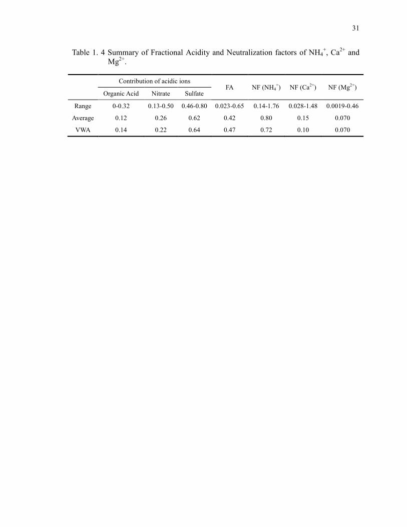
The acidity in precipitation at Newark was mainly caused by H2SO4, with HNO3
and organic acids as major additional contributors. As shown in Table 1.4, SO42-
contributed more than half of the acidity (64% of the total), while NO3- and organic acid
contribute 22% and 14% of the total acidity, respectively. This finding is consistent with
the conclusions of Kaya and Tuncel (1997) and similar to the work by Keene et al (1986)
who predicted that organic acid may account for ~15% of the total acidity for North
America. Compared with other regions, the H2SO4 contribution to the acidity is higher
(Al-Momani et al., 1995; Tuncer et al., 2001) while HNO3 contribution is lower
(Migliavacca et al., 2005) in this study area, indicating reduced NOx emission. These
results suggest that the source strength of each contributing acidic species varies,
contributing differently to the precipitation acidity at this location.
To better understand the precipitation acidity, Fractional Acidity (FA)
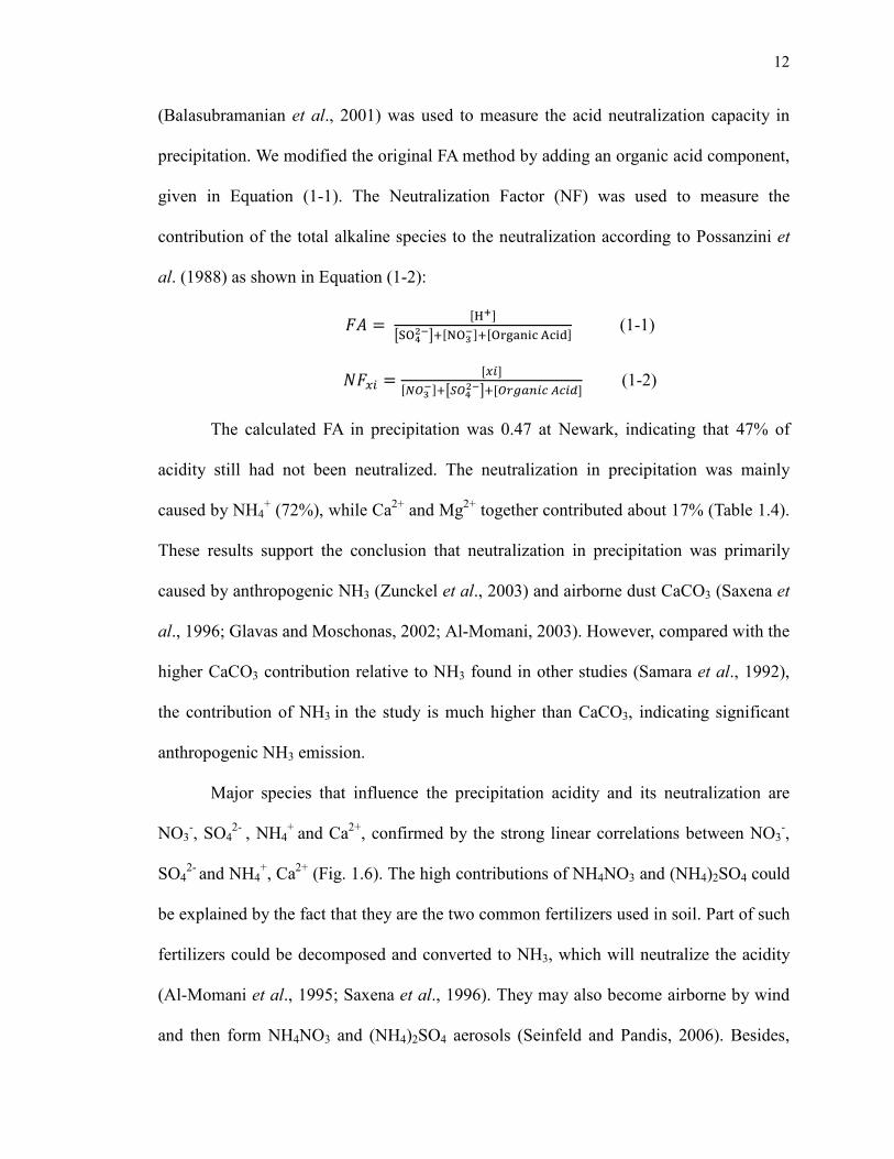
12
(Balasubramanian et al., 2001) was used to measure the acid neutralization capacity in
precipitation. We modified the original FA method by adding an organic acid component,
given in Equation (1-1). The Neutralization Factor (NF) was used to measure the
contribution of the total alkaline species to the neutralization according to Possanzini et
al. (1988) as shown in Equation (1-2):
�� = ����
�� �������
����������� ����� (1-1)
���� = ��������
��� �� �����!"#$�% &%�'�
(1-2)
The calculated FA in precipitation was 0.47 at Newark, indicating that 47% of
acidity still had not been neutralized. The neutralization in precipitation was mainly
caused by NH4+ (72%), while Ca
2+ and Mg
2+ together contributed about 17% (Table 1.4).
These results support the conclusion that neutralization in precipitation was primarily
caused by anthropogenic NH3 (Zunckel et al., 2003) and airborne dust CaCO3 (Saxena et
al., 1996; Glavas and Moschonas, 2002; Al-Momani, 2003). However, compared with the
higher CaCO3 contribution relative to NH3 found in other studies (Samara et al., 1992),
the contribution of NH3 in the study is much higher than CaCO3, indicating significant
anthropogenic NH3 emission.
Major species that influence the precipitation acidity and its neutralization are
NO3-, SO4
2- , NH4
+ and Ca
2+, confirmed by the strong linear correlations between NO3
-,
SO42-
and NH4+, Ca
2+ (Fig. 1.6). The high contributions of NH4NO3 and (NH4)2SO4 could
be explained by the fact that they are the two common fertilizers used in soil. Part of such
fertilizers could be decomposed and converted to NH3, which will neutralize the acidity
(Al-Momani et al., 1995; Saxena et al., 1996). They may also become airborne by wind
and then form NH4NO3 and (NH4)2SO4 aerosols (Seinfeld and Pandis, 2006). Besides,

13
emissions from fossil fuel combustion could also contribute to the NH3 production
(Ugucione et al., 2002). Previous studies suggest that ammonium salts produced from
reaction with NH3 are the most important acidity-controlling chemicals (Langford et al.,
1992; Lee and Atkins, 1994).
1.3.3. Enrichment Factor Analysis
Enrichment Factors (EFs), a first-step source estimator of chemical components in
precipitation (Chabas and Lefevre, 2000; Okay et al., 2002), was employed in this study
to explore the possible sources: anthropogenic, marine or crust origins. For seawater EFs,
Na was used as a reference element (Keene et al., 1986); while Al was selected as a
reference to crust sources The EFs were calculated via following equations:
(� )#*#+)!,-./ = ,�� �#0 /1234515676589
,�� �#0 /:37;7632 (1-3)
(�<!=>+,-./ = ,�� &?0 /1234515676589
,�� &?0 /42@:6 (1-4)
In these equations, the ratios (xi/Na)Seawater are taken from Keene et al. (1986), and
(xi/Al)Crust are taken from Weaver and Tamey (1984), and Taylor and McLennan (1985).
Based on the rules of Poissant et al. (1994), EFs between 1 and 10 suggest the major
influence of marine or soil sources; when EFs range between 10-500, moderate
enrichments are indicated, while when EFs are over 500, extreme enrichments exist.
As shown in Table 1.5, the EFSeawater for Na+, Cl
-, Mg
2+ and K
+ ranged from 1 to
10, suggesting a marine origin, mainly sea salt aerosols emitted from seawater (Zunckel
et al., 2003; Migliavacca et al., 2004). This conclusion is further confirmed by strong
correlations between Cl- and Na
+ and between Cl
- and K
+ (Fig. 1.7). The Ca
2+ ion is
moderately enriched compared with both seawater and crustal sources, with its EFSeawater ,
EFcrustal being 28.4 and 51.2 respectively, suggesting that Ca2+
in precipitation may

14
mainly derived from both the marine and crustal sources, especially the marine source.
Meanwhile the anthropogenic sources could also contribute and thus lead to the moderate
enrichment factors.
For trace elements in precipitation measured at this location, the crustal EFs
calculations show that Fe, Co and Al mainly originate from crust sources. The elements
Ca2+
, K+, Na
+, Mg
2+, Pb, V, Cr, Ni are moderately enriched, with EFs being from 43 (V)
to 414 (Pb). Apparently the moderate enrichment of Ca2+
, Na+, K
+ and Mg
2+ is mainly
caused by sea salt related sources, as indicated by their low EFNa values. K+ may also be
emitted from forest fires and soil re-suspension (Đorđević et al., 2005). Pb, V, Cr, Ni may
come from high temperature combustion processes (Lindberg, 1982; Scudlark et al., 1994)
and traffic emissions (Al-Momani, 2003). The elements Sb, Cu, Zn, Cd, Cl- and F
- are
highly enriched, with EFs ranging from 714 (Cu) to more than 105 (Cl
-). For the most
enriched Cl-, in addition to the marine source, other anthropogenic sources may also
contribute (Safai et al., 2004; Migliavacca et al., 2005). The highly enriched fluoride may
originate from fertilizer production and coal-fired power plant emissions (Zunckel et
al.,2003; Migliavacca et al.,2004 ), and Sb could be derived from fly ash generated
during combustion processes (Velzen et al., 1998). The high enrichment of Zn could be
contributed by road traffic emissions (Steven et al., 1997; Al-Momani, 2003) and hospital
waste burning (Sanusi et al., 1996). The extremely high enrichments of Cu and Cd are
mainly caused by both lower and high temperature combustion processes, such as
incineration (Pio et al., 1996; Al-Momani, 2003).
1.3.4. Factor Analysis
To explore the correlations among observed variables and potential major sources

15
of chemical species in precipitation at this location, Factor Analysis was carried out. Six
major factors were extracted from the 25 observed variables, with the prominent
variables in bold (Table 1.6). The six factors together explain 83.9% of the total
variations caused by all variables.
F1, with high loading of Al, Cr, Fe, Co, F-, NO3
-, NH4
+ and Ca
2+, may represent a
mixed source involving natural crustal material weathering and agricultural practices,
considering that Fe, Al, Co are mainly of typical crust origin and NH4NO3 is a major
component in fertilizers used in agriculture. F- may also come from fertilizer industry
related processes; Cr and Ca2+
probably came from crust sources or soil fertilization. F2
mainly consists of SO42−
, NH4+, H
+ and three organic acids (acetate, formic acid and
oxalate), representing the end-products of secondary reaction processes that control the
alkalinity-acidity equilibrium. SO42-
and NH4+ are the two major secondary pollutants
controlling the alkalinity-acidity equilibrium. The association of the three organic acids
with F2 indicates their important contribution to the acidity. NO3- is not associated with
F2, suggesting that it may play less of a role in the alkalinity-acidity equilibrium. In
contrast to the results of Avila and Alarco (1999) and Tang et al., (2005), both alkaline
and acidic secondary chemicals affecting the alkalinity-acidity equilibrium are included
in F2, and in particular, NH4+ is the dominant alkaline species in this study. F3 represents
the marine source with high loading of Cl-, Mg
2+, Na
+, consistent with previous works
(Lee et al, 2000; Mihajlidi-Zelić et al., 2006). F4 is characterized by the high
contributions of Sb, Pb, Zn and Cd, attributed to possible fossil fuel burning and
incineration processes (Scudlark et al., 1994; Pio et al., 1996; Al-Momani, 2003). F5 has
high loadings of Ni and K+, representing oil combustion processes and biomass burning.

16
Ni is mainly from oil combustion processes (Lee and Duffield, 1977). For K+, it could be
emitted from either oil combustion or biomass burning processes (Zunckel et al., 2003;
Khare et al., 2004). F6 has malonate and vanadium as prominent variables, representing
other either natural or anthropogenic sources that are enriched with both species; this
finding is unique at the site and may need further studies. The six factors could explain
23.9%, 19.2%, 14.6%, 12.0%, 7.7% and 6.5% of the total chemical composition
variations, respectively (Table 1.6).
1.3.5. Cluster analysis
To characterize the source-precipitation event relationships as a function of the
seasons, cluster analysis was carried out, using Ward’s method to minimize the sum of
the squares of any two hypothetical clusters that can be formed at each step (Ward, 1963)
in order to emphasize the homogeneous nature of each cluster. This method is different
from the cluster analysis commonly used in other studies that compute the square
Euclidean distances between samples by K-mean clustering technique using chemicals’
concentration data (Avila and Alarco, 1999; Gao and Anderson, 2001; Glavas and
Moschonas, 2002). We used the 6 selected factors in cluster analysis instead of the
original concentration data to reduce noise caused by errors in the original data.
All precipitation events were grouped into 6 clusters and their dominant
influencing factors could be interpreted as: (1) well-mixed sources, (2) nitrogen-enriched
soil, (3) marine sources, (4) secondary pollution processes, (5) incineration, oil
combustion processes and (6) a combination of nitrogen-enriched soil and malonate-
vanadium-enriched sources.
Different clusters of the precipitation events showed different air-mass

17
transportation patterns, as shown by the back-trajectory paths under NOAA HYSPLIT
Model in Fig. 1.8. In the study, a 72 hours period of were selected for the back-trajectory
considering the lifetime of the different secondary species (Wojcik and Chang, 1997).
Usually for the precipitation events in cluster 3, which was interpreted as marine source,
the air mass at the selected height of 20m, 500m and 2000m were mainly from the
Atlantic Ocean, while for other precipitation events their air mass were mainly originated
from the continent. The results of the back-trajectory shown in Fig. 1.8 supported well
the result of cluster analysis and could indicate the potential geographic origins of the
pollutants in the precipitation. In addition, the results of wind direction were found to
influence the characteristic of precipitation (Fig. 1.9). For the precipitation in cluster 3,
the corresponding wind direction were mainly east to south (Oct. 4, 2006 and Nov. 16,
2006 as examples), while for the other precipitation, the wind direction were mainly from
east direction (Oct. 20, 2006 and Nov. 2, 2006 as examples). At last, Wind speed could
not influence the chemical characteristic of the precipitation obviously.
After cluster analysis, the characteristics of precipitation during each season, with
possible sources, are summarized in Table 1.7. About half of the precipitation events were
classified into C1, indicating that mixed sources contribute greatly to precipitation events
all year around. The other half of the precipitation events were controlled by specific
sources in different seasons. Many events are grouped into C2 in springtime, which are
associated with nitrogen-enriched soil sources. In summer, both C4 and C5 dominated the
precipitation events associated with secondary pollution, incineration and oil combustion
processes. In autumn, marine sources indicated by C3 influenced greatly the chemical
characteristics of precipitation. In winter, mixed sources played the major role.

18
1.4. Conclusions
Results from this study on precipitation chemistry carried out during 2006-2007
in Newark, NJ lead to the following conclusions:
SO42-
and NH4+ are the two most dominant components of major ions in mass,
accounting for 50.5% of the total anions and 48.6% of total cations, respectively. Al
(33.6%), Zn (26.8%) and Fe (25.2%) are the three most abundant trace metals in
precipitation. Organic acid mass in precipitation is predominately composed of acetate
(42.0%) and formate (40.2%).
The precipitation at Newark showed an acidic nature, with VWA pH ~ 4.6. The
acidity is caused mainly by SO42-
(64%), with NO3- (22%) and organic acid (14%) as
additional acidity contributors. About 47% of the acidity was neutralized by NH4+, Ca
2+
and Mg2+
; in particular NH4+
contributed as much as 72% of the total neutralization.
Marine, continental crust and anthropogenic sources showed significant influence
on the chemical composition of precipitation at this location. Na+, Cl
-, Mg
2+ and K
+ are
primarily of marine origin and Fe, Co and Al are mainly from crust sources. Due to the
anthropogenic influences, Pb, V, Cr, Ni are moderately enriched while Zn, Sb, Cu, Cd and
F- are highly enriched.
Based on factor analysis, six major sources were found to control the
characteristics of precipitation: (1) nitrogen-enriched soil, (2) secondary pollution
processes, (3) marine sources, (4) incineration processes, (5) oil combustion and (6)
malonate-vanadium-enriched sources, together explaining ~ 83.9% of the variations of 25
variables.
The results of cluster analysis show that about half of the precipitation events

19
were controlled by mixed sources while for the rest of the precipitation events, their
major sources showed obvious seasonality. In spring, nitrogen-enriched soil contributed
much. During summer, secondary pollution, incineration and oil combustion showed
great influences, while marine sources influenced the precipitation composition
significantly during autumn. In winter, however, no specific sources controlled the
characteristics of precipitation.

20
1.5. References
Al-Momani, I. F., 2003. Trace elements in atmospheric precipitation at Northern Jordan
measured by ICP-MS: acidity and possible sources. Atmos. Environ 37, 4507–4515.
Al-Momani, I.F., Tuncel, S., Eler, U., Ortel, E., Sirin, G., Tuncel, G., 1995. Major ion
composition of wet and dry deposition in the eastern Mediterranean basin. Sci. Total
Environ 164, 75–85.
Avila, A., Alarcon, M., 1999. Relationship between precipitation chemistry and
meteorological situations at a rural site in NE Spain. Atmos Environ 33:1663–77.
Ayars, J., Gao Y., 2007. Atmospheric nitrogen deposition to the Mullica River-Great Bay
Estuary. Marine Environmental Research 64, 590-600.
Balasubramanian, R., Victor, T., Chun, N., 2001. Chemical and statistical analysis of
precipitation in Singapore. Water, Air, and Soil Pollution 130, 451–456.
Basak, B., Alagha, O., 2004. The chemical composition of rainwater over Buyukcekmece
Lake, Istanbul. Atmos. Res 71, 275–288.
Chabas, A., Lefevre, R.A., 2000. Chemistry and microscopy of atmospheric particulates
at Delos (Cyclades—Greece). Atmos. Environ 34, 225–238.
Das, R., Das, S.N., Misra, V.N., 2005. Chemical composition of rainwater and dustfall at
Bhubaneswar in the east coast of India. Atmos. Environ 39, 5908–5916.
Dasch, J.M., Wolff, G., 1989. Trace inorganic species in precipitation and their potential
use in source apportionment studies. Water, Air, and Soil Pollution 43, 401–412.
Deboudt, K., Flament, P., Laure Bertho, M., 2004. Cd, Cu, Pb and Zn concentrations in
atmospheric wet deposition at a coastal station in Western Europe. Water, Air, and
Soil Pollution 151, 335–359.

21
Đorđević, D., Mihajlidi-Zelić, A., Relić, D., 2005. Differentiation of the contribution of
local resuspension from that of regional and remote sources on trace elements
content in the atmospheric aerosol in the Mediterranean area. Atmos Environ 39:
6271–81.
G. Brooks A. J., Kieber, R. J., Witt, M., Willey J. D., 2006. Rainwater monocarboxylic
and dicarboxylic acid concentrations in southeastern North Carolina, USA, as a
function of air-mass back-trajectory. Atmos. Environ 40, 1683-1693.
Gao, Y., 2002. Atmospheric nitrogen deposition to Barnegat Bay. Atmos. Environ 36,
5783–5794.
Gao Y., Anderson R. A., 2001. Characteristics of Chinese aerosols determined by
individual-particle analysis. Jouornal of Geophysical Research 106, 18037–18045
Glavas, S., Moschonas, N., 2002. Origin of observed acidic–alkaline rains in a wet-only
precipitation study in a Mediterranean coastal site, Patras, Greece. Atmos Environ
36, 3089–99.
Goncalves, F.L.T., Massambani, O., Beheng, K.D., Vautz, W., Schilling, M., Solci, M.C.,
Rocha, V., Klockow, D., 2000. Modelling and measurements of below cloud
scavenging processes in the highly industrialized region of Cubatão-Brazil. Atmos.
Environ 34, 4113–4120.
Goncalves, F.L.T., Ramos, A.M., Freitas, S., Silva Dias, M.A., Massambani, O., 2002. In-
cloud and below-cloud numerical simulation of scavenging processes ata Serra do
Mar region, SE Brazil. Atmos. Environ 36, 5245–5255.
Heaton, R.W., Rahn, K.A., Lowenthal, D.H., 1990. Determination oftrace elements,
including regional traces, in Rhode Island precipitation. Atmos. Environ 24A (1),

22
147–153.
Herut, B., Nimmo, M., Medway, A., Chester, R., Krom, M.D., 2001. Dry atmospheric
inputs oftrace metals at the Mediterranean coast ofIsrael (SE Mediterranean):
sources and fluxes. Atmos. Environ 35, 803–813.
Heuer, K., Tonnessen, K.A., Ingersill, G.P., 2000. Comparison of precipitation chemistry
in the Central Rocky Mountains, Colorado, USA. Atmos. Environ 34, 1713–1722.
Hou, H., Takamatsu, T., Koshikawa, M. K., Hosomi, M., 2005. Trace metals in bulk
precipitation and throughfall in a suburban area ofJapan. Atmos. Environ 39, 3583–
3595.
Hu, G.P., Balasubramanian, R., Wu, C.D., 2003. Chemical characterization of rainwater
at Singapore. Chemosphere 51, 747–755.
Huang, X., Hu, M., He, L., Tang, X., 2005. Chemical characterization of water-soluble
organic acids in PM2.5 in Beijing, China. Atmos. Environ 39(16): 2819-2827.
Huang, Y., Wang, Y., Zhang, L., 2008. Long-term trend of chemical composition of wet
atmospheric precipitation during 1986-2006 at Shenzhen city, China, Atmos.
Environ., doi:10.1016/j. atmosenv.2007.12.063.
Injuk, J., van Grieken, R.V., 1995. Atmospheric concentrations and deposition ofheavy
metals over the North Sea: a literature review. Journal of Atmospheric Chemistry 20,
179–212.
Ito, M., Mitchell, M., Driscoll, C.T., 2002. Spatial patterns of precipitation quantity and
chemistry and air temperature in the Adirondack region of New York. Atmos.
Environ 36, 1051–1062.
Kanellopoulou, E.A., 2001. Determination of heavy metals in wet deposition of Athens.

23
Global Nest: The International Journal 3 (1), 45–50.
Keene, W.C., Galloway, J.N., Holden, J.D., 1983. Measurement of weak organic acidity
in precipitation from remote areas of the world. J. Geophys. Res 88, 5122–5130.
Keene, W.C., Galloway, J.N., 1984. Organic acidity of precipitation of North America.
Atmos. Environ 18, 2491–2497.
Keene,W.C., Pszenny, A.P., Gallloway, J.N., Hawley, M.E., 1986. Sea salt correction and
interpretation of constituent ratios in marine precipitation. J. Geophys. Res 91,
6647–6658.
Khare, P., Goel, A., Patel, D., Behari, J., 2004. Chemical characterization of rainwater at
a developing urban habitat of Northern India. Atmos. Res 69, 135–145.
Kim, G., Scudlark, J. R., Church, T. M., 2000. Atmospheric wet deposition of trace
elements to Chesapeake and Delaware Bays. Atmos. Environ 34, 3437 – 3444.
Langford, A. O., Fehsenfeld, F. C., Zachariassen, J., Schimel, D. S., 1992. Gaseous
ammonia fluxes and background concentrations in terrestrial ecosystems in the
United States. Glob Biogeochem Cycles 6, 459–483.
Lara, L. B. L. S., Artaxo, P., Martinelli, L.A., Victoria, R.L., Camargo, P.B., Krusche, A.,
Ayres, G.P., Ferraz, E.S.B., Ballester, M.V., 2001. Chemical composition of
rainwater and anthropogenic influences in the piracicaba river basin, Southeast
Brazil. Atmospheric Environment 35, 4937–4945.
Le Bolloch, O., Guerzoni, S., 1995. Acid and alkaline deposition in precipitation on the
western coast of Sardinia, central Mediterranean (401N, 81E). Water, Air, and soil
pollution 85, 2155–2160.
Lee, R.E. Jr., Duffield, F.V., 1977. EPA’s catalyst research program: environmental

24
impact of sulfuric acid emissions. J. Air Pollut. Control Assoc. 27, 631-635.Lee, D.
S., Atkins, D. H. F., 1994. Atmospheric ammonia emissions from agricultural waste
combustion. Geophys Res Lett 21, 281–284.
Lee, B.K., Hong, S.H., Lee, D.S., 2000. Chemical composition of precipitation and wet
deposition of major ions on the Korean peninsula. Atmos. Environ 34, 563–575.
Lindberg, S.E., 1982. Factors influencing trace metal, sulfate, and hydrogen ion
concentration in rain. Atmos. Environ 16, 1701-1709.
Migliavacca, D., Teixeira, E.C., Wiegand, F., Machado, A. C. M., Sanchez, J., 2005.
Atmospheric precipitation and chemical composition of an urban site, Guaiba
hydrographic basin, Brazil. Atmos. Environ 39, 1829–1844.
Migliavacca, D., Teixeira, E. C., Pires, M., Fachel, J., 2004. Study of chemical elements
in atmospheric precipitation in South Brazil. Atmos. Environ 38, 1641–1656.
Mihajlidi-Zelić, A., Deršek-Timotić, I., Relić, D., Popović, A., Đorđević, D., 2006.
Contribution of marine and continental aerosols to the content of major ions in the
precipitation of the central Mediterranean. Science of the Total Environment 370,
441–451.
Nriagu, J.O., Pacyna, J.M., 1988. Quantitative assessment o worldwide contamination of
air, water, and soils by trace metals. Nature 333, 134-139.
Okay, C., Akkoyunlu, B.O., Tayanc, M., 2002. Composition of wet deposition in
Kaynarca, Turkey. Environ. Pollut 118, 401–410.
Paerl, H.W., 1985. Enhancement of marine primary production by nitrogen enriched acid
rain. Nature 315, 747–749.
Pelicho, A. F., Martins, L. D., Nomi, S. N., Solci, M. C., 2006. Integrated and sequential

25
bulk and wet-only samplings of atmospheric precipitation in Londrina, South Brazil
(1998–2002). Atmos. Environ 40, 6827–6835.
Pena, R.M., Garcia, S., Herrero, C., Losada, M., Vazquez, A., Lucas, T., 2002. Organic
acids and aldehydes in rainwater in a northwest region of Spain. Atmos. Environ 36,
5277–5288.
Pike, S.M., Moran, S.B., 2001. Trace elements in aerosol and precipitation at New Castle,
NH, USA. Atmos. Environ 35, 3361–3366.
Pio, C.A., Castro, L.M., Cerqueira, M.A., Santos, I.M., Belchior, F., Salgueiro, M.L.,
1996. Source assessment of particulate air pollutants measured at the southwest
European coast. Atmos. Environ 30 (19), 3309–3320.
Poissant, L., Schmit, J.P., Beron, P., 1994. Trace inorganic elements in rainfall in the
Montreal Island. Atmos. Environ 28, 339–346.
Possanzini, M., Buttini, P., Dipalo, V., 1988. Characterization of a rural area in terms of
dry and wet deposition. Sci. Total Environ 74, 111–120.
Rastogi, N., Sarin, M.M., 2005. Chemical characteristics of individual rain events from a
semi-arid region in India: three-year study. Atmos. Environ 39, 3313–3323.
Taylor, S.R., McLennan, S.M., 1985. The continental crust: Its composition and evolution,
Blackwell Sci. Publ., Oxford, 330.
Safai, P.D., Rao, P.S.P., Momin, G.A., Ali, K., Chate, D.M., Praveen, P.S., 2004.
Chemical composition of precipitation during 1984–2002 at Pune, India. Atmos.
Environ 38, 1705–1714.
Samara, C., Tsitouridou, R., Balafoutis, C., 1992. Chemical composition of rain in
Thessaloniki, Greece, in relation meteorological conditions. Atmos. Environ 26B,

26
359 –367.
Sanusi, A., Wortham, H., Millet, M., Mirabel, P., 1996. Chemical composition of
rainwater in eastern France. Atmos. Environ 30, 59–71.
Saxena, A., Kulshrestha, U. C., Kumar, N., Kumari, K. M., Srivastava, S. S., 1996.
Characterization of precipitation at Agra. Atmos Environ 30, 3405–12.
Scudlark, J.R., Conko, K.M., Church, T.M., 1994. Atmospheric wet deposition of trace
elements to Chesapeake Bay: CBAD study year 1 results. Atmos. Environ 28, 1487-
1498.
Seinfeld, J. H., Pandis, S. N., 2006. Atmospheric Chemistry and Physics From Air
Pollution to Climate Change, John Wiley & Sons, Inc., Hoboken, New Jersey, 294–
299, 336-337.
Spanos, T., Simeonov, V., Andreev, G., 2002. Environmetric modeling of emission
sources for dry and wet precipitation from an urban area. Talanta 58, 367–375.
Steven, H.C., Mulawa, P.A., Balli, J., Donase, C., Weibel, A., Sagebiel, J.C., 1997.
Environmental Science and Technology 31, 3405.
Tang, A., Zhuang G., Wang Y., Yuan H., Sun Y., 2005. The chemistry of precipitation and
its relation to aerosol in Beijing. Atmos. Environ 39, 3397–3406.
Topcu, S., Incecik, S., Atimtay, A., 2002. Chemical composition of rainwater at EMEP
station in Ankara, Turkey. Atmospheric Research 65, 77–92.
Tuncer, B., Bayer, B., Yesilyurt, C., Tuncel, G., 2001. Ionic composition of precipitation
at the central Anatolia, Turkey. Atmos. Environ 35, 5989–6002.
Ugucione, C., Felix, E.P., Rocha, G.O., Cardoso, A.A., 2002. Daytime and nighttime
removal processes of atmospheric NO2 and NH3 in Araraquara’s region - SP.
27
Ecletica Quimica 27, 1–9.
Velzen, D. V., Langenkamp, H., Herb, G., 1998. Antimony, its sources, applications and
flow paths into urban and industrial waste: a review. Waste Management &
Research 16(1), 32-40.
Ward, J. H., 1963. Hierachical grouping to optimize an objective function. J. Am. Statist.
Assoc. 58, 236-244.
Weaver, B.L., Tamey, J., 1984. Major and trace element composition of the continental
lithosphere. Physics and Chemistry of the Earth, 39-68.
Wojcik G.S. and Chang J.S., 1997. A re-evaluation of sulphur budgets, lifetimes, and
scavenging ratios for eastern north America. Journal of Atmospheric Chemistry 26,
109–145.
Yu, S., Gao, C., Cheng, Z., Cheng, X., Cheng, S., Xiao, J., Ye, W., 1998. An analysis of
chemical composition of different rain types in ‘Minnan Golden Triangle’ region in
the southeastern coast of China. Atmos. Res., 47–48, 245–269.
Zhao, Y., Gao, Y., 2008. Mass size distributions of water-soluble inorganic and organic
ions in size-segregated aerosols over metropolitan Newark in the US east coast.
Atmos. Environ , doi:10.1016/j.atmosenv.2008.01.032.
Zunckel, M., Saizar, C., Zarauz, J.,2003. Rainwater composition in Northeast Uruguay.
Atmos Environ 37, 1601–1611.

28
Table 1. 1 Summary of major anions, cations concentrations and pH in precipitation
(ppm).
Chemicals pH Cl- F
- �O3
- SO4
2− �H4
+ Ca
2+ Mg
2+ K
+ �a
+
Minimum* 3.83 0.07 <0.00 0.32 0.37 0.02 0.04 <0.00 <0.00 0.03
Maximum* 6.36 3.35 0.13 4.23 8.92 1.73 1.67 0.28 0.18 2.04
Mean* 4.57 1.08 0.03 1.38 2.64 0.64 0.21 0.05 0.06 0.60
VWA* 4.60 0.38 0.02 0.89 1.83 0.44 0.12 0.04 0.05 0.25
SD* 0.45 0.71 0.04 0.98 1.90 0.41 0.26 0.06 0.04 0.44
Spring Mean* 4.84 0.44 0.04 1.3 2.00 0.66 0.37 0.05 0.07 0.26
Summer Mean* 4.34 0.36 0.01 1.5 3.66 0.72 0.18 0.03 0.06 0.14
Fall Mean* 4.56 0.89 0.04 1.21 2.37 0.53 0.15 0.08 0.07 0.59
Winter Mean* 4.67 1.06 0.03 1.75 1.75 0.63 0.13 0.04 0.07 0.62
Shenzhen, Chinaa - 1.34 0.09 1.37 7.14 0.63 3.11 0.24 0.28 0.93
Adirondack, �Yb 6.62 0.08 - 1.40 3.54 0.19 0.14 0.02 0.01 0.04
Great Bay, �Jc 4.32 9.47 - 2.33 2.88 0.42 - - - 2.07
�orthern Jordand - 1.31 - 4.68 5.97 0.27 4.33 0.75 0.43 1.15
Galiee, Isracle 6.26 6.25 - 1.74 14.44 0.44 1.79 0.68 0.14 3.82
Singaporef - 0.78 - 1.04 5.64 0.31 0.87 0.19 0.15 0.71
Ankara, Turkeyg - 0.72 - 1.81 4.61 1.56 2.86 0.23 0.38 0.36
Spainh - 1.01 - 1.28 4.43 0.41 2.30 0.24 0.16 0.51
Italyi - 11.42 - 1.80 8.65 0.45 2.81 1.87 0.66 5.79
Central-
Mediterraneanj
- 4.90 - 2.97 12.75 0.79 5.91 1.42 0.85 5.42
*The study region; aHuang et al., (2008);
bIto et al., (2002);
cAyars and Gao,
dAl-
Momani, (2003); eHerut et al., (2000);
fBalasubramanian et al., (2001);
gTopcu et al.,
(2002); hAvila and Alarcon, (1999);
iLe Bolloch and Guerzoni, (1995);
jMihajlidi-Zelić et
al., (2006).

29
Table 1. 2 Summary of trace metals concentrations in precipitation (ppb).
Chemicals Sb Pb Al V Cr Fe Co �i Cu Zn Cd
Min* 0.06 0.03 0.90 0.02 <0.01 <0.01 <0.01 0.07 0.05 1.22 <0.01
Max* 2.10 1.97 31.68 0.69 0.33 43.20 0.11 1.51 64.32 16.95 0.21
Mean* 0.36 0.47 9.54 0.28 0.06 8.35 0.02 0.55 2.82 6.60 0.03
VWA* 0.27 0.39 6.09 0.24 0.07 4.57 0.01 0.45 1.15 4.86 0.02
SD* 0.36 0.45 8.50 0.18 0.06 10.52 0.03 0.28 56.46 4.40 0.04
Spring Mean* 0.55 0.53 9.58 0.20 0.06 7.25 0.03 0.37 1.86 8.61 0.04
Summer Mean* 0.32 0.48 11.45 0.27 0.05 11.48 0.02 0.70 1.45 7.25 0.03
Fall Mean* 0.27 0.39 7.50 0.33 0.03 5.42 0.02 0.52 1.20 4.59 0.02
Winter Mean* 0.29 0.51 9.86 0.39 0.07 10.19 0.03 0.62 1.13 6.31 0.01
�orthern Jordana 0.16 2.57 382.00 4.21 0.77 92.00 - 2.62 3.08 6.52 0.42
Mediterraneanb - 6.20 - - - - - - 13.60 2.60 0.40
Athensc - 0.88 - - - 4.38 - 4.14 15.41 33.46 0.20
Western Europed - 2.80 - - - - - 1.40 21.80 0.11
Western Massache 0.23 4.50 53.00 1.10 0.14 65.00 - 0.75 0.95 3.70 0.31
Rhode Islandf 0.05 - 71.00 0.80 - 38.00 - - - 4.50 -
�ew Castle, USj - - 24.00 - - 23.00 - - 1.30 26.00 -
Montreal,
Canadah
0.25 - 18.00 - - 91.00 - - 4.00 28.00 -
*The study region; a
Al-Momani, (2003); bMihajlidi-Zelić et al., (2006);
cKanellopoulou, (2001);
dDeboudt et al., (2004);
eDasch and Wolff, (1989);
fHeaton et al.,
(1990); gPike and Moran, (2001);
hPoissant et al., (1994).

30
Table 1. 3 Concentrations of selected organic acids in precipitation at Newark (ppm).
Chemicals Ac- HCOO
− CH2(COO)2
2− C2O4
2−
Minimum* <0.01 <0.01 <0.01 <0.01
Maximum* 1.13 0.82 0.31 0.22
Mean* 0.25 0.22 0.03 0.06
VWA* 0.21 0.20 0.03 0.06
Spring Mean* 0.16 0.24 0.04 0.08
Summer Mean* 0.48 0.40 0.05 0.10
Fall Mean* 0.11 0.10 0.01 0.02
Winter Mean* 0.16 <0.01 0.04 0.02
SD* 0.27 0.23 0.06 0.06
California, USAa 0.43 0.45 0.072 0.16
*This work; a G. Brooks et al., (2006).
31
Table 1. 4 Summary of Fractional Acidity and Neutralization factors of NH4+, Ca
2+ and
Mg2+
.
Contribution of acidic ions
FA NF (NH4+) NF (Ca
2+) NF (Mg
2+)
Organic Acid Nitrate Sulfate
Range 0-0.32 0.13-0.50 0.46-0.80 0.023-0.65 0.14-1.76 0.028-1.48 0.0019-0.46
Average 0.12 0.26 0.62 0.42 0.80 0.15 0.070
VWA 0.14 0.22 0.64 0.47 0.72 0.10 0.070

32
Table 1. 5 Summary of Enrichment Factors.
EFSeawater EFCrust
Sb 73100 25300
Pb 1070000 414
Al 446000 1.00
V 12500 42.8
Cr 14500 49.0
Fe 197000 0.89
Co 5510 4.78
�i 12700 136
Cu 6200 714
Zn 64500 1280
Cd 16300 3140
Cl- 1.42 107000
F- 1320 1170
Ca2+
28.4 51.2
Mg2+
1.48 44.8
K+ 8.99 60.5
�a+ 1.00 397

33
Table 1. 6 Varimax Rotated Factor Loadings.
F1 F2 F3 F4 F5 F6
Sb 0.395 0.117 -0.205 0.759 0.017 -0.171
Pb 0.548 0.024 -0.183 0.683 0.078 -0.272
Al 0.825 0.341 -0.122 0.242 0.193 -0.038
V 0.243 0.212 -0.566 0.102 0.113 -0.51
Cr 0.77 0.17 -0.109 0.365 0.136 -0.241
Fe 0.766 0.347 -0.097 0.293 0.103 -0.267
Co 0.867 -0.021 0.013 0.187 0.024 -0.025
Ni 0.147 -0.011 -0.001 0.23 0.865 -0.271
Cu 0.486 -0.015 -0.111 0.528 0.474 -0.236
Zn 0.439 0.165 0.013 0.601 0.383 0.101
Cd -0.01 0.029 0.023 0.845 0.147 0.196
CH3COO− -0.05 0.86 0.204 0.074 -0.003 -0.293
Cl- 0.053 -0.241 -0.942 0.077 0.02 -0.064
F- 0.698 -0.379 -0.023 -0.297 0.074 0.082
HCOO− 0.014 0.883 0.264 0.069 -0.068 -0.058
CH2(COO)22−
0.075 0.383 0.127 -0.052 0.128 -0.582
NO3- 0.753 0.423 -0.208 0.161 0.17 -0.245
C2O42−
0.235 0.827 0.191 0.021 -0.017 0.171
SO42−
0.41 0.721 -0.176 0.074 0.269 -0.221
NH4+ 0.603 0.609 -0.174 0.079 0.34 0.073
Ca2+
0.749 0.371 -0.245 0.219 0.122 0.273
Mg2+
0.156 -0.034 -0.941 0.051 0.084 0.171
K+ 0.276 0.243 -0.465 0.134 0.644 0.272
Na+ 0.056 -0.269 -0.939 0.047 0.033 -0.025
H+ 0.279 0.75 -0.011 0.074 0.129 -0.44
Eigen Values 5.97 4.81 3.65 2.99 1.93 1.63
%Variance 23.9% 19.2% 14.6% 12.0% 7.7% 6.5%

34
Table 1. 7 Scores of selected clusters model and seasonal distribution of precipitation
events.
CLUSTER Significant Factors
included
*Precipitation events distribution
Spring Summer Autumn Winter
C1 F1, F2, F3, F4, F5 3 7 9 3
C2 F1 4 1 - -
C3 F3 - - 5 -
C4 F2 - 4 - -
C5 F4, F5 1 3 1 -
C6 F1, F6 - - - 1
*4 precipitation events with missing variables were not included

35
Figure 1. 1 Map of sampling location.

36
Total Annions (µeq/L)
0 100 200 300 400 500 600 700
Tota
l C
ati
on
s (µ
eq/L
)
0
100
200
300
400
500
600
700y = 1.00x - 8.37
R2 = 0.875
Figure 1. 2 Electric charge equilibrium between total anions and total cations.

37
Organic Acid13.8%
Sulfate50.5%
Chloride10.6%
Fluoride0.5%
Nitrate24.6%
(a)
Oxalate11.4
Formate40.2
Malonate6.4
Acetate42.0
(d)
Ammonium48.6
Calcium13.5
Magnesium4.5
Sodium27.9
Potassium5.5
(b)
Al33.6%
Pb2.1%Cd0.1%
Fe25.2%
Ni2.5%
Cu6.4%
Sb1.5%
Cr0.4%
Zn26.8%
V1.3%
(c)
Figure 1. 3 Pie charts of Anions, Cations, Trace Metals and Organic Acid, shown in (a),
(b), (c), (d) respectively.

38
R2=0.26
Precipitation (cm)0 5 10 15
Tra
ce M
eta
l (p
pb
)
0
20
40
60
80
100
R2 = 0.18
Ino
rga
nic
An
nio
ns
(pp
m)
0
2
4
6
8
10
12
14R
2= 0.32
Ino
rga
nic
Ca
tio
ns
(pp
m)
0.0
0.5
1.0
1.5
2.0
2.5
3.0
3.5
4.0
Precipitation (cm)0 5 10 15
Org
an
ic A
cid
(p
pm
)0.0
0.5
1.0
1.5
2.0
2.5
3.0
(a) (b)
(d)(c)
Figure 1. 4 Dilution effect of Precipitation volume on total anions (a), total cations (b),
trace metals (c) and Organic Acid (d).
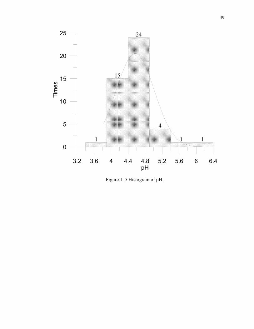
39
3.2 3.6 4 4.4 4.8 5.2 5.6 6 6.4pH
0
5
10
15
20
25
Tim
es
1
15
24
4
1 1
Figure 1. 5 Histogram of pH.

40
�O3
- (µeq/L)
0 20 40 60 80
�H
4
+ (
µeq
/L)
0
50
100
150
200
250
y= 0.29x+ 2.49
R 2 = 0.52
Ca
2+ (
µeq
/L)
0
10
20
30
y = 0.90x +21.18
R2
= 0.60
SO4
2- (µeq/L)
0 50 100 150 200
y = 0.09x + 3.80
R2
= 0.32
y = 2.44x +16.05
R2
= 0.71
Figure 1. 6 Correlations between major cations NH4+, Ca
2+ and major anions NO3
- and
SO42-
.

41
Cl- ( µeq/L )
0 20 40 60 80 100
�a
+
( µ
eq/L
)
-20
0
20
40
60
80
100
y = 0.95x -2.42
R2
= 0.98
0 20 40 60 80 100
K+ (
µeq
/L )
0
5
10
15
20
25
y = 0.20x + 0.40
R2 = 0.72
Cl- ( µeq/L )
Figure 1. 7 Correlations between Cl- and Na
+, K
+ in precipitation.
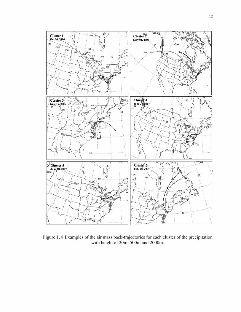
42
Figure 1. 8 Examples of the air mass back-trajectories for each cluster of the precipitation
with height of 20m, 500m and 2000m.

43
Figure 1. 9 Examples of the wind speed and wind directions in precipitation periods.

44
Chapter 2 . Size Distributions of Trace Elements Associated with
Ambient Particular Matter in the Affinity of Highways
in the New Jersey-New York Metropolitan Area on the
US East Coast*
* This work has been submitted to Atmospheric Environment and it is under review as of
April, 16th 2011.

45
Abstract
To characterize the size distributions of trace elements associated with particulate
matter in the areas heavily impacted by traffics, 11 sets of size segregated aerosol
samples were taken using a MOUDI sampler in winter and summer of 2007-2008 along
the side of a highway in the northeast New Jersey near New York City. Selected trace
metals (Al, Cd, Co, Cr, Cu, Fe, Mn, Ni, Pb, Sb, Sc, V and Zn) in aerosol samples were
determined by ICPMS. Results showed that the concentrations of these elements varied
seasonally. A typical mass-size bimodal distribution with peaks at the size range of 0.32-
0.56µm and 3.2-5.6µm was identified, and the general size distributions of the mass
concentrations did not change significantly with seasons. Trace metals of potential
anthropogenic origin, including Cd, Fe, Ni, Pb, Zn, Sb and Co, had higher concentrations
and enrichment levels in winter, especially for fine particles. For trace metals of crustal
origin, such as Fe and Sc, their size distributions of enrichment factors showed significant
seasonal variations while no such variations found for anthropogenic trace metals such as
Cd, Cr, Ni, Pb, Sb, V, Zn and Co. The size distributions of trace metal enrichment factors
showed primarily monotonic decline patterns with overwhelmingly high peaks in the size
range of 0.18-0.32 µm for most of the trace metals from pollution sources. Crustal
elements, including Fe, Cu (summer), Mn (summer) and Sc (winter), however, showed
tilted normal distributions pattern with peaks at 1.0-1.8 µm. Two groups of size
distributions in trace metal concentrations were identified using cluster analysis: (1)
coarse particles (>1.0µm) with accumulation of mainly crustal trace metals such as Al, Fe,
Sc, and Mn; (2) fine particles (<1.0µm) with accumulations of trace metals of
anthropogenic origins such as Cd, Pb, Ni, V and Co. Three major types of sources for

46
these metals were identified at this location: (1) brake wear, fuel combustion, (2) primary
fuel combustion, and (3) tire abrasion and fuel combustion. The particulate trace metals
in the study area are primarily characterized by either the mixed sources or the exhaust
emissions source. Weather factors, in particular temperature, wind speed and precipitation,
were found to significantly (α = 0.05) influence the concentrations of trace metals and
their size distributions.
Key Words: Size distributions, trace metals, urban air pollution, traffic emission.

47
2.1. Introduction
Atmospheric trace metals and their size distributions in particulate matters can
influence both human health and ecology environment (Berggren et al., 1990; Hinds,
1999; Ghio et al., 1999; Allen et al., 2001; Gao et al., 2002). By inhalation and respiration,
airborne particles enriched with potentially toxic trace metals could deposit in human
body and cause chronic and acute health problems (Chapman et al., 1997; Wichmann and
Peters, 2000; Stieb et al., 2002, Pope et al., 2002). The particle size is an important factor
controlling the deposition efficiency of trace metals (Hinds, 1999), and thus can influence
greatly on the trace metals’ toxicity effects (Allen et al., 2001). Previous studies found
that the finer the particle, the deeper it could be deposited in the human body, and thus
the more serious damages it could cause (Oberdorster et al., 2005; Karakoti et al., 2006;
Ntziachristos et al., 2007). However, the knowledge for different trace metals
accumulations in human bodies remains limited due to the lack of information on their
size distributions and processes affecting their size characteristics such as aerosol aging,
sources, and the ambient atmospheric conditions (Ondov and Wexler, 1998; Birmill et al.,
2006). On the other hand, the air born trace metals in aerosols could also affect the
terrestrial and coastal ecosystems via air-to-land and air-to-sea deposition (Church et al.,
1984; Yang et al., 1996; De Vries and Bakker, 1996; Allen et al., 2001), and the size of
atmospheric particles is an important factor affecting the rate of atmospheric dry
deposition and their life time in the atmosphere (Jaenicke, 1998; Allen et al., 2001;
Ntziachristos et al., 2007). Moreover, the extent of direct and indirect aerosol radioactive
forcing in the earth climate system is largely dependent on the size distributions of
aerosol particles, and some elements in aerosols, such iron oxides minerals, may affect

48
significantly on light absorption (Lafon et al., 2006). Therefore characterizing the size
distributions of trace elements in aerosol particles is relevant to climate studies (IPCC,
2001).
The size distributions of trace metals in aerosols are mainly controlled by their
sources, life time in the atmosphere, and the meteorological conditions (Kuhn et al., 2005;
Seinfeld and Pandis, 2006; Ntziachristos et al., 2007). Trace metals from anthropogenic
sources tend to accumulate in fine mode (<1.0µm) (Allen et al., 2001), while the crustal
sources contribute to trace elements mainly in coarse mode (>1.0µm) (Handler et al.,
2008). After particulate matter being emitted into the atmosphere, the sizes of particles
may increase by coagulation or decrease due to evaporation of the water content in
particles (Zhang and Wexler, 2004), resulting the changes in the size distributions.
Besides, meteorological parameters, such as wind speed, temperature and relative
humidity, could also influence the size distributions of trace metals in aerosols (Zhang et
al., 2004; Kuhn et al., 2005). Therefore, the size distributions of trace metals in aerosols
are the reflection of multiple chemical and physical processes occurring in the
atmosphere.
In urban regions, vehicle related emissions including fuel combustion, tire
abrasion and brake wear, and the re-suspension of road dust, are among the important
sources of trace metals in the ambient air (Handler et al., 2008). Particularly, the vehicle
exhausts from fuel combustion could contribute greatly to the enrichment of Cu, Fe, and
Sb in aerosol particles (Pakkanen et al., 2003; Ntziachristos et al., 2007). The brake wear
are also among the important sources of Pb and Mn. (Garg et al., 2000; Young et al.,
2002). Besides, the additives such as Ca and Mg in motor oils could be the potential

49
sources for these elements in the air (Cadle et al., 1997). In general, the fine mode
particles were found mainly derived from combustion processes, while the coarse
particles are mainly come from the road dust re-suspensions and abrasions processes
(Handler et al., 2008). However, the smallest size of road dust particles may extent to
about 0.1µm that could also contribute to the mass of fine particles (Kleeman and Cass,
1998).
Although the mass size distributions of aerosols and associated trace metals in the
ambient air have been studied in some regions (Berggren et al., 1990; De Vries and
Bakker, 1996; Allen et al., 2001; Pakkanen et al., 2003; Ntziachristos et al., 2007;
Handler et al., 2008), such studies, in particular in the affinity of heavy traffics, are
limited in the US east coast region. The size distributions of trace metals enrichment
factors and their potential sources categories still need further investigations. To fill the
data gap in trace metal size-distributions in this region and to provide insights into the
metal-health relationships, we carried out an ambient aerosol measurement focusing on
the characteristics of trace metals in different size fractions. A total of 11 sets of size
segregated aerosol samples were collected at the road side of the New Jersey Turnpike,
one of the busiest highways in New Jersey-New York City metropolitan area. The
objectives of this study are: (1) to characterize the mass size distribution of particulate
mass and associated trace metals, (2) to investigate the enrichment levels of trace metals
in size segregated aerosol particles and their size distributions, (3) to identify the major
categories of sources contributing to the enrichments of trace metals, and (4) to explore
the influences of weather conditions on the concentrations of selected trace metals and
their size distributions.
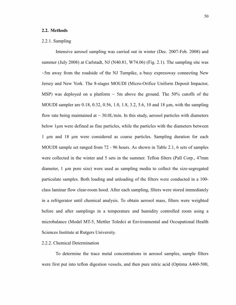
50
2.2. Methods
2.2.1. Sampling
Intensive aerosol sampling was carried out in winter (Dec. 2007-Feb. 2008) and
summer (July 2008) at Carlstadt, NJ (N40.81, W74.06) (Fig. 2.1). The sampling site was
~5m away from the roadside of the NJ Turnpike, a busy expressway connecting New
Jersey and New York. The 8-stages MOUDI (Micro-Orifice Uniform Deposit Impactor,
MSP) was deployed on a platform ~ 5m above the ground. The 50% cutoffs of the
MOUDI sampler are 0.18, 0.32, 0.56, 1.0, 1.8, 3.2, 5.6, 10 and 18 µm, with the sampling
flow rate being maintained at ~ 30.0L/min. In this study, aerosol particles with diameters
below 1µm were defined as fine particles, while the particles with the diameters between
1 µm and 18 µm were considered as coarse particles. Sampling duration for each
MOUDI sample set ranged from 72 - 96 hours. As shown in Table 2.1, 6 sets of samples
were collected in the winter and 5 sets in the summer. Teflon filters (Pall Corp., 47mm
diameter, 1 µm pore size) were used as sampling media to collect the size-segregated
particulate samples. Both loading and unloading of the filters were conducted in a 100-
class laminar flow clear-room hood. After each sampling, filters were stored immediately
in a refrigerator until chemical analysis. To obtain aerosol mass, filters were weighted
before and after samplings in a temperature and humidity controlled room using a
microbalance (Model MT-5, Mettler Toledo) at Environmental and Occupational Health
Sciences Institute at Rutgers University.
2.2.2. Chemical Determination
To determine the trace metal concentrations in aerosol samples, sample filters
were first put into teflon digestion vessels, and then pure nitric acid (Optima A460-500,
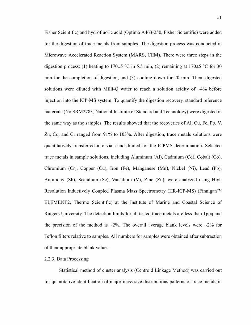
51
Fisher Scientific) and hydrofluoric acid (Optima A463-250, Fisher Scientific) were added
for the digestion of trace metals from samples. The digestion process was conducted in
Microwave Accelerated Reaction System (MARS, CEM). There were three steps in the
digestion process: (1) heating to 170±5 °C in 5.5 min, (2) remaining at 170±5 °C for 30
min for the completion of digestion, and (3) cooling down for 20 min. Then, digested
solutions were diluted with Milli-Q water to reach a solution acidity of ~4% before
injection into the ICP-MS system. To quantify the digestion recovery, standard reference
materials (No.SRM2783, National Institute of Standard and Technology) were digested in
the same way as the samples. The results showed that the recoveries of Al, Cu, Fe, Pb, V,
Zn, Co, and Cr ranged from 91% to 103%. After digestion, trace metals solutions were
quantitatively transferred into vials and diluted for the ICPMS determination. Selected
trace metals in sample solutions, including Aluminum (Al), Cadmium (Cd), Cobalt (Co),
Chromium (Cr), Copper (Cu), Iron (Fe), Manganese (Mn), Nickel (Ni), Lead (Pb),
Antimony (Sb), Scandium (Sc), Vanadium (V), Zinc (Zn), were analyzed using High
Resolution Inductively Coupled Plasma Mass Spectrometry (HR-ICP-MS) (Finnigan™
ELEMENT2, Thermo Scientific) at the Institute of Marine and Coastal Science of
Rutgers University. The detection limits for all tested trace metals are less than 1ppq and
the precision of the method is ~2%. The overall average blank levels were ~2% for
Teflon filters relative to samples. All numbers for samples were obtained after subtraction
of their appropriate blank values.
2.2.3. Data Processing
Statistical method of cluster analysis (Centroid Linkage Method) was carried out
for quantitative identification of major mass size distributions patterns of trace metals in

52
aerosols. In this procedure, the concentrations of trace metals in atmosphere were first
normalized to relative concentrations by setting the peak concentration in one sample set
as 1 and the concentrations of other size ranges were converted to the ratios to its peak
concentration, using the following equation:
ABCDEFGHIJ KG = KG DELMNGNO KG0 (2-1)
where i is integer from 1 to 8 representing the 8 different size fractions in one sample set.
The major size distributions of the trace metal enrichment levels were also distinguished
by cluster analysis, using the normalized enrichment factor values which were calculated
similarly to the above method. At last, Factor Analysis (Principal Component Analysis,
Varimax Rotation) was employed to identify the potential major sources of those trace
metals associated with particulate matter in the study area. The cluster analysis and factor
analysis were accomplished in MinTab 14 Statistical Software (Minitab Inc.) and SAS
9.1 (SAS).
2.3. Results
2.3.1. Concentrations and Seasonal Variations
The concentrations of trace metals in all size ranges showed seasonal variability,
especially for those associated with fine mode particles as indicated by the Relative
Standard Variations (RSV) in Table 2.2. This pattern may be due to the seasonal
variation of local source emissions and regional weather conditions. The concentrations
of the typical crustal elements, such as Al, in both fine and coarse mode particles, were
mainly higher in summer, while for other trace metals, possibly dominated from
anthropogenic sources, such as Cd, Cr, Cu, Fe, Ni, Pb, Zn, Sb, Co and Mn, their
relatively high concentrations happened in winter, even though the total mass

53
concentrations were higher in summer (Table 2.2).
The seasonal RSV of trace metals in coarse particles ranged from 3% to 51%,
varying among different metals. The concentrations of Co and Sc did not show
significant seasonal variations, while Cd, Ni and Zn were found with RSV ~ 50%,
indicating the significant seasonal variation of their sources. In the fine mode particles,
the seasonal RSV of the concentrations of most trace metals (Al, Cd, Cr, Pb, V, Zn, Sc,
Co) were found higher compared with those in coarse mode particles, ranging from 2% to
more than 100%. Besides the seasonal variations, the inter-seasonal variations of the
concentrations in each season were also observed (Table 2.2). Compared with coarse
particles in summer, the variations of trace metal concentrations on the event-basis were
higher in fine particles and in winter. Such variations could be caused by the instability of
source emissions and the ambient atmospheric conditions (Ondov and Wexler, 1998;
Seinfeld and Pandis, 2006). During the winter time, the Al, Cd, Pb and Cu showed more
inter-seasonal variations in both fine and coarse mode particles, while in summer only Cu
showed significant inter-seasonal variations.
2.3.2. Trace Metal Enrichment Factors
To estimate the strength of the crustal source influences, the crustal enrichment
factors of trace elements were calculated based on Equation (2-2).
PQRF,SG/ =,SG RF0 /TUMV
,SG RF0 /KCWXY (2-2)
where ,X� Al0 /]�^_` is the average ratios of the element of interests (X) and crustal
representative element (Al) (Turekian and Wedepohl,1961; Ronov and Yaroshevsky, 1969;
Weaver and Tamey, 1984; and Taylor,1985). The EFs calculations indicate that common
crustal elements (Fe, Sc and Mn) and Co were relatively lowly enriched, while all the

54
other trace metals were enriched from medium to high levels, primarily from
anthropogenic sources. According to their crustal Enrichment Factors (EFs) in both fine
and coarse particles (Table 2.3), the extents of the enrichment of trace metals with respect
to the crustal source were grouped into three levels: (1) Low Enrichment (EFs<10), (2)
Medium Enrichment (10< EFs<100), and (3) High Enrichment (EFs>100).
The enrichment factors of trace metals showed significant seasonal variations
with much higher enrichment levels happened in winter for trace metals in both fine and
coarse modes (Table 2.3), indicating possibly more contributions from anthropogenic
pollution sources in that season. In addition, the magnitude of such seasonal variations
was different between fine particles and coarse particles. Compared with coarse particles
mainly from re-suspension of road dust and soil particles (Handler et al., 2008), trace
metals in the fine mode showed more increased enrichments in winter. This suggests that
the enhanced vehicle fuel combustion and domestic heating in winter could contribute
more to the enrichments of trace metals in fine mode particles.
2.4. Discussions
2.4.1. Mass Size Distributions of Particulate Matter
A bimodal size distribution of the aerosol mass concentrations was observed in
both winter and summer at this location (Fig. 2.2). The pattern of mass size distributions
was consistent between winter and summer at a similarity level of 98.2% (Table 2.4). The
two peaks were centered at ~0.32-0.56µm in fine mode particles and ~3.2-5.6µm in
coarse mode particles. The aerosol mass was slightly more accumulated in fine particles
than in coarse particles, accounting for about 56% and 54% of the total mass in winter
and summer, respectively, different to the fine-particles dominating pattern in urban

55
Newark, NJ (Zhao and Gao, 2008) that the fine particles accounted for 64–82% of the
total mass. In addition, different to the results of Zhao and Gao (2008) that mass
concentrations of aerosol particles in all size ranges in winter were lower than those in
summer, the mass concentrations at each size range observed in this study showed no
significant seasonal variations, suggesting that the constant vehicle emissions at this site
could dominate the aerosol mass in its affinity area and thus obscure the possible seasonal
variations of mass concentrations caused by other factors. This comparison provides
different aerosol size-distribution characteristics between an urban center and intensive
vehicle emission location. On the other hand, results from this study is consistent to the
conclusion of Zhao and Gao (2008) that local ambient conditions and in situ production
mechanisms could be more important to the evolution of the observed mass size
distributions.
Significant differences in the size distributions during different sampling events
were found, especially in summer. The similarity levels of the distributions for different
sampling events were 82% and 75% in winter and summer, respectively (Table 2.4),
suggesting the variability in mass size distributions of particulate matter on a short-term
basis. As shown in Fig. 2.2, the mass size distributions of samples #1 (in winter) and #7
(in summer) were shifted from the averaged distributions of other samples, which suggest
the fluctuations of the ambient conditions on daily and weekly basis that impact the size
distributions of particulate matter at this location. Many factors including the mixing
layer height changes, emission intensity variations and seasonality of air mass origins
may jointly contribute to the observed differences (Gerasopoulos et al., 2007; Venzac et
al., 2009).

56
2.4.2. Mass Size Distributions of Trace Metals
The mass size distributions of trace metals did not vary significantly between
winter and summer at this location, probably due to the fact that the sampling site is close
to the highway thus the dominating traffic related emissions could cover the seasonality;
however the variability of the mass size distributions of these metals in each season were
high, especially in winter (Table 2.4). The mass size distributions of Co and Cd showed
more seasonal variations while the seasonal variations of Ni and V were small. This may
indicate that the source types in both seasons for Ni and V were similar and that the in
situ situations such as weather conditions could not significantly change the mass size
distributions of Ni and V. Most trace metals, especially Cd, Cr, Cu and Zn, showed more
variations in their mass size distributions in winter, indicating their major contributing
sources varied more in winter than in summer. Besides, the meteorological parameters
(Temperature, Wind Speed and Humidity) changed substantially (Table 2.1) due to the
longer span of sampling period (Dec-Feb) in winter than that in summer (July), which
could attributed to the observed variations. In summer, Pb and Zn also showed high
variations in their mass size distributions.
The mass size distributions of trace metals could be characterized into 2 groups
based on the results of cluster analysis: Group I- coarse particles accumulations
dominated in particles larger than 1µm and Group II- fine particle accumulations
dominated in particles of smaller than 1µm. Then three clusters were derived from each
group (Table 2.5 and Fig. 2.3). All potential crustal trace metals including Al, Fe, Sc and
Mn were included in Group I, and most of the potentially anthropogenic trace metals
such as Cd, Pb, Ni, V and Co were categorized in Group II. This is consistent with the

57
size distribution characteristics of both crustal and anthropogenic trace metals found in
other locations (Allen et al., 2001; Singh et al., 2002; Pakkanen et al., 2003).
In general, the mass size distributions in Group I showed bimodal patterns with
primary peak at the size range of 3.2-5.6 µm, and secondary peak at the size range of 1.0-
1.8 µm (Fig. 2.3), and this was divided further into three clusters (1, 2, 3)(Table 2.5; Fig.
2.4). Cluster 1, consisted with crustal trace metals (Al, Fe, Sc and Mn) and Cr in both
winter and summer, was characterized by relatively higher primary peak while the
secondary peak was much lower. For the trace metals in Cluster 2 (Cu and Sb), the
secondary peak was almost as high as the primary peak, showing a typical bimodal
pattern. The size distribution of Co in summer was similar to that of Cluster 1 except for
the peak at size range of 0.18-0.32 µm, and thus it was distinguished from other elements
and stood alone as Cluster 3. The mass size distributions of trace metals in Group II that
was also further divided into three clusters (4, 5, 6) were mainly characterized by a
decreasing trend in size from fine to coarse modes, with a major peak at 0.18-0.56 µm
(Fig. 2.4). The mass size distribution of Cd in winter, the only element in Cluster 4, was
unique and characterized by a bimodal distribution with the primary peak at the size
range of 0.56-1.0 µm and secondary peak at 3.2-5.6 µm. The Pb and Zn in both seasons
and Cd in summer were grouped into Cluster 5, which was characterized by three
decreasing peaks at the size ranges of 0.32-0.56 µm, 1.0-1.8 µm and 3.2-5.6 µm,
respectively. The trace metals in Cluster 6 also showed a decreasing pattern in mass size
distributions with a high peak at 0.18-0.32µm, although a smaller peak existed at the size
range of 3.2-5.6 µm in the distributions. The Ni, V in both seasons and Co in winter were
included in Cluster 6.

58
Compared with previous studies, different mass size distributions for Zn, Co, Cu,
Pb, Sb, Ni, and V were found at this location (Fig. 2.4). The accumulation levels of these
metals in fine particles were relatively high compared with the results from other regions,
such as the United Kingdom (Allen et al., 2001), Los Angeles Basin (CA) in the US
(Singh et al., 2002) and Finland (Pakkanen et al., 2003). Besides, the Pb, Zn, Co, Ni and
V showed the highest accumulation levels at the size range of 0.18-0.32µm in the fine
particles, while for Cu and Sb the accumulation levels at each size range of fine particles
were similar. These results indicated the characteristics of the traffic related trace metal
pollutions and the important contributions of combustion exhaust emissions, which will
be discussed further Section 4.4 of this paper.
2.4.3. Enrichment Factor Size Distributions of Trace Metals
In-season and seasonal variations of the EF size distributions of trace metals were
different for both crustal elements (Cu, Fe and Sc) and trace metals of potential
anthropogenic origins (Cd, Cr, Ni, Sb, V, Zn and Co), as shown in Table 2.3. In general,
the EF size distributions of trace metals for potential crustal trace metals showed much
higher seasonal and in-season variations. Compared with summer, the intra-season
variations of the EF size distributions were greater in winter. While for anthropogenic
trace metals, both the seasonal and intra-season variations of EF size distributions were
much less, indicating that the anthropogenic sources of trace metals did not change much
during different seasons or sampling events since the vehicle related emissions were the
major sources. Comparatively, the intra-season variations of the EF size distributions
were higher in summer.
For most trace metals, the EF size distributions were found approximately a

59
monotonic decline pattern with highest enrichment level in very fine particulate, except
some common crust originated metals such as Fe, Mn, Sc (winter) and Cu (summer).
This is consistent to the previous findings that most trace metals are more enriched in fine
particulate matter in urban regions dominated by anthropogenic emissions (Bayens and
Dedeurwaerder, 1991; Chan et al., 1997; Wang et al., 2006). As shown in Fig. 2.5, 3
clusters were identified representing the major EF size distributions of trace metals using
normalized EFs data. Both Clusters 1 and 2 showed tilted normal distributions with peak
at the size range of 1.0-1.8 µm. However, for Cluster 1, the trace metals in fine particles
were more enriched than in coarse mode, while the reverse situations were observed for
Cluster 2. The common potential crustal elements Fe, Sc (winter), Mn and Cu (summer)
were the major trace metals that showed EF size distributions of cluster 1 and 2,
indicating the possibly less influence caused by fine particle related vehicle direct
emissions via fuel combustion, and this was consistent with their low enrichment levels
(Table 2.3). The EF size distributions for the other trace metals fell into the Cluster 3,
which showed overwhelmingly high peak at the size of 0.18-0.32 µm and decreasing
enrichment levels from small to big particles size. Besides, a tiny peak may also occur in
the size range of 0.56-1.8 µm for the EF size distributions of Cluster 3. The differences in
the enrichment levels of these trace elements across a wide range of particle sizes indicate
the different sources, transportation and production processes for these elements (Birmili
et al., 2006; Moreno et al., 2006; Chen et al., 2008).
2.4.4. Trace Metal Sources Identification
Using the concentrations data of trace metals in both fine and coarse particles,
Factors Analysis (with Principal Component Factor Analysis and Varimax Rotation

60
methods) was employed to find the latent underlying factors which account for the
correlations among observed trace metals, thus to better explain the potential sources for
these trace metals. As shown in Table 2.6, three factors were extracted that represent
different types of sources relating to traffic emissions, with the key elements highlighted
in bold: Factor 1, brake wear, fuel combustion, and urban pollutions; Factor 2, primary
fuel combustion; and Factor 3, tire abrasion and fuel combustion. The factor analysis
divided the traffic pollution into two main emission types successfully: exhaust and non-
exhaust pollution that will be discussed in more details below. In addition, it also divided
the non-exhaust emissions into two major types: brake ware emissions and tires abrasion
emissions (Thorpe and Harrison, 2008). A total of 86.9% variations could be explained by
the extracted 3 major source categories.
Fuel combustion (known as “exhaust emissions”), which was found contributing
to all 3 major sources, was exclusively dominate in Factor 2, while brake wear and tire
abrasions were the major non-exhaust emission sources represented in Factors 1 and 3.
Factor 1 was characterized by Fe, Sb, Pb and Cd. Fe and Sb are the two most common
trace metals found in brake related emissions caused by frictional contacts between brake
systems components (Thorpe and Harrison, 2008; Gietl et al., 2010). In addition, Pb
could also be originated from brake wares related emissions (Garg et al., 2000; Young et
al., 2002; Pakkanen et al., 2003). However, the direct vehicle emissions could also
generate Fe, Sb, Pb and Cd pollution (Pacyna, 1986; Garg et al., 2000; Young et al., 2002;
Pakkanen et al., 2003; Ntziachristos et al., 2007). Sb and Cd were commonly found in the
urban industry processes such as high temperature combustion and waste incineration
(Pacyna, 1998; Gao et al., 2002). The trace metals charactering Factor 1 explained ~35%

61
variations of trace metals. The Factor 2 included Cr, Ni, V and Cu, which were primarily
emitted from vehicle fuel combustion processes (Pacyna, 1998; Ntziachristos et al., 2007).
A total of ~28.3% variations of trace metals concentrations observed at this location
could be explained by the Factor 2. Zn and Co, both are additives of tires and road
marking paint (Sorme et al., 2001), were coupled together, serving as Factor 3, which
explained ~23.7% variations. The tire abrasion emission has been recognized as an
important source of Zn, and a significant amountof this element was found in re-
suspended tire abrasions (Adachi and Tainosho, 2004, Councell et al., 2004, Schauer et
al., 2006). In addition, Zn and Co could also from fuel combustion of different kinds
(Pacyna, 1998; Weckwerth, 2001; Al-Momani, 2003). In summary, the three factors
identified in this study could explain ~86.9% variations of trace metals observed at this
location.
To further characterize the sources of each sampling event, cluster analysis was
carried out using the Ward's method. We used the results from factor analysis instead of
the original concentration data to reduce noise caused by errors in the original data (Song
and Gao, 2009). Four cluster were extracted (Table 2.7), with their dominant influencing
factors being interpreted: Cluster 1 with no specific source factors dominating in summer;
Cluster 2 with exhaust emissions as the dominant source in winter; Clusters3 and Cluster
4, with each including only one sample set and having brake wear and tire abrasion as a
dominant source. This indicates that the dominant source for most air born trace metals at
this location is traffic emissions, although other sources also exist. As shown in Fig. 2.6,
the air mass back trajectories calculated by the NOAA HYSPLIT model indicate that the
air mass for Cluster 1 was mainly from marine/coast or rural regions, which could reduce

62
the impact of local traffic emissions on the concentrations of trace metals in the ambient
air. For Cluster 2, its air mass came mainly from the long-distance east/northeast urban
areas, and thus could change the atmospheric characteristics of trace metals from local
traffic pollution, as the combustion related fine particles could be transported from other
urban regions into this area and thus increase the dominance of such source observed at
this site. For Clusters 3 and 4, the air mass mainly originated from neighbor states in
relatively short-distance, New York and Pennsylvania, and the short-distance transport
may increase the chance of the transport of large aerosol particles, adding to the
accumulation of trace metals associated with coarse particles mainly from local brake
wear and tire abrasion. Therefore, the concentrations and size characteristics of trace
metals observed at this location were affected by many sources.
2.4.5. Weather Influence on Trace Metal Concentrations and Size Distributions
The differences of trace metals concentrations and size distributions in different
events and seasons indicated significant (α = 0.05) influences from weather conditions
such as temperature, wind speed and precipitation. As shown in Table 2.8, the
temperature could influence significantly trace metals concentrations in both coarse and
fine particulate, especially in fine particulate mode. In particular, common anthropogenic
trace metals (Pb, Zn, Co, Ni) showed negative concentration-temperature correlations,
which could be explained by the influence of ambient temperature on vehicle exhaust
emissions (Mulawa and Cadle, 1997). Wind speed was found of effective effects to
reduce the air mass and trace metals concentrations in roadside region because of the
potential disperse effects. As shown in Table 2.8, the high wind speed tends to
accumulate trace metals (such as Al, Pb and Sc) in fine particulate mode, and the high

63
precipitation volume tends to accumulate trace metals (such as Al, V and Sc) in coarse
particulate mode. However, local wind direction was not found of obvious influences on
trace metal concentrations and size distribution. On the other hand, the precipitation
could also reduce the air mass and trace metals concentrations effectively because of the
flushing effects, especially for fine particles as shown in Table 2.8. The weather
influences on the concentrations of trace metal differed at different size ranges, thus
leading to the change of its size distributions.
2.5. Conclusions
Results from this study on size distribution characteristics of trace metals and
their enrichment factors carried out during 2007-2008 in Carlstadt, NJ lead to the
following conclusions:
The mass size distributions in both seasons showed typical bimodal patterns, with
peaks in the size ranges of 0.32-0.56µm and 3.2-5.6µm. The vehicle related emissions
could be influential to the mass concentrations of particulate matter in the ambient air.
The patterns of mass size distributions of trace metals did not show significant
seasonal variations; however, the concentrations of trace metals in all size ranges showed
seasonal variations, especially for trace metals in fine particles. In both fine and coarse
particles, the concentrations of crustal elements such as Al and Sc were higher in summer
while the typical anthological elements Cd, Fe, Ni, Pb, Zn, Sb and Co showed higher
concentrations in winter. The elements, Zn, Co, Cu, Pb, Sb, Ni, and V, were found of
more accumulated in fine mode.
The enrichment factors of trace metals showed different seasonal variations in
different size ranges, with higher enrichment levels in winter than in summer, especially

64
for fine particles. For crustal trace metals such as Cu, Fe, Sc, their EF size distributions
showed large seasonal variations, while no such obvious variations were found with
anthropogenic trace metals including Cd, Cr, Ni, Pb, Sb, V, Zn and Co. The EF size
distributions of most trace metals showed a monotonic decline pattern. Specifically, 3
clusters of the major EF size distributions patterns were identified: (1) declined normal
distribution with fine particles accumulations and peak in 1.0-1.8 µm for Cu (summer)
and Fe (winter); (2) inclined normal distribution with coarse particles accumulations and
peak in 1.0-1.8 µm for Fe (summer), Sc (winter) and Mn (summer); (3) monotonic
decline patterns with overwhelming peak in 0.18-0.32 µm for rest of trace metals.
Using cluster analysis method, the mass size distributions of the 13 trace metals
were characterized into 2 groups: (1) coarse particle accumulation with crustal trace
metals such as Al, Fe, Sc and Mn, showing bimodal pattern with primary peak at the size
range of 3.2-5.6 µm, and secondary peak at 1.0-1.8 µm range; (2) fine particle
accumulation for most of the typical anthropogenic trace metals such as Cd, Pb, Ni, V
and Co, showing decreasing concentrations from small to large particles with major peaks
at 0.18-0.32 µm range.
Three primary sources explaining a total of ~86.9% variations in trace metal
mass-size distributions were: (1) brake wear, fuel combustion and urban pollutions, (2)
primary fuel combustion, and (3) tire abrasion and fuel combustion. Weather parameters,
in particular temperature, wind speed and precipitation, were found to be effective on the
concentrations and size distributions of trace elements observed at this location.

65
Acknowledgment
This work was sponsored by The US EPA with the Award #XA97268501.
Additional support was provided by Rutgers University through a New Faculty Start-up
Fund to YG. We thank Jin Young Shin, Christopher Thuman, and Irene Jung for
assistance with sampling and M. Paul Field and Christine Theodore for assistance with
ICPMS analysis. We are grateful to Francisco Artigas and Christine Hobble for the
operation of the sampling sites during this study.

66
2.6. References
Adachi, K., Tainosho, Y., 2004. Characterization of heavy metal particles embedded in
tire dust. Environment International 30, 1009-1017.
Allen, A.G., Nemitz, E., Shi, J.P., Harrison, R.M., Greenwood, J.C., 2001. Size
distribution of trace metals in atmospheric aerosols in the United Kingdom.
Atmospheric Environment 35, 4581-4591.
Al-Momani, I. F., 2003. Trace metals in atmospheric precipitation at Northern Jordan
measured by ICP-MS: acidity and possible sources. Atmospheric Environment 37,
4507–4515.
Bayens, W., Dedeurwaerder, H., 1991. Particulate trace metals above the southern bight
of the north sea - II. Origin and behaviour of the trace metals. Atmospheric
Environment 25, 1077–1092.
Berggren, D., Bergkvist, B., Falkengrengrerup, U., Folkeson, L., Tyler, G., 1990. Metal
solubility and pathways in acidified forest ecosystems of south Sweden. Science of
the Total Environment 96, 103–114.
Birmili, W., Allen, A.G., Bary, F., Harrison, R.M., 2006. Trace Metal Concentrations and
Water Solubility in Size-Fractionated Atmospheric Particles and Influence of Road
Traffic. Environ. Sci. Technol. 40 (4), 1144–1153.
Cadle, S.H., Mulawa, P.A., Hunsanger, E.C., Nelson, K., Ragazzi, R.A., Barrett, R.,
Gallagher, G.L., Lawson, D.R., Knapp, K.T., Snow, R., 1999. Composition of light-
duty motor vehicle exhaust particulate matter in the Denver, Colorado area.
Environmental Science and Technology 33, 2328–2339.
Chan, Y.C., Simpson, R.W., McTainsh, G.H., Vowles, P.D., Cohen, D.D., Bailey, G.M.,

67
1997. Characterisation of chemical species in PM2.5 and PM10 aerosols in
Brisbane, Australia. Atmospheric Environment 31, 3773–3785.
Chapman, R.S., Watkinson, W.P., Dreher, K.L., Costa, D.L., 1997.Ambient particulate
matter and respiratory and cardiovascular illness in adults: particle-borne transition
metals and the heart–lung axis.Environ mental Toxicology and Pharmacology 4 (3–
4), 331–338.
Chen, Y., Paytan, A., Chase, Z., Measures, C., Beck, A. J., Sañudo-Wilhelmy, S. A. and
Post A. F., 2008, Sources and fluxes of atmospheric trace elements to the Gulf of
Aqaba, Red Sea, J. Geophys. Res., 113, D05306, doi:10.1029/2007JD009110.
Church, T.M., Tramontano, J.M., Scudlark, J.R., Jickells, T.D., Tokos, J.J., Knap, A.H.,
1984. The wet deposition of trace metals to the Western Atlantic Ocean at the Mid-
Atlantic coast and on Bermuda. Atmospheric Environment 18, 2657–2664.
Councell, T.B., Duckenfield, K.U., Landa, E.R., Callender, E., 2004. Tire-wear particles
as a source of zinc to the environment. Environmental Science & Technology 38,
4206-4214.
De Vries, W., Bakker, D.J., 1996. Manual for calculating critical loads of heavy metals
for soils and surface waters. Report 114, DLO, Winland Staring Centre,
Wageningen, The Netherlands.
Duce, R.A., Hoffman, G.L., Zoller, W.H., 1975. Atmospheric trace metals at remote
northern and southern hemisphere sites: pollution or natural? Science 187, 339–342.
Gao, Y., Nelson, E.D., Field, M.P., Ding, Q., Li, H., Sherrell, R.M., Gigliotti, C.L., Van
Ry, D.A., Glenn, T.R., Eisenreich, S.J., 2002. Characterization of atmospheric trace
metals on PM2.5 particulate matter over the New York–New Jersey harbor estuary.

68
Atmospheric Environment 36, 1077–1086.
Garg, B.D., Cadle, S.H., Mulawa, P.A., Groblicki, P.J., Laroo, C., Parr, G.A., 2000. Brake
wear particulate matter emissions. Environmental Science and Technology 34,
4463–4469.
Gerasopoulos, E., Koulouri, E., Kalivitis, N., Kouvarakis, G., Saarikoski, S., Makela, T.,
Hillamo, R., Mihalopoulos, N., 2007. Size-segregated mass distributions of aerosols
over Eastern Mediterranean: seasonal variability and comparison with AERONET
columnar size-distributions. Atmospheric Chemistry and Physics 7, 2551–2561.
Ghio, A.J., Stonehuerner, J., Dailey, L.A., Carter, J.D., 1999. Metals associated with both
the water-soluble and insoluble fractions of an ambient air pollution particle
catalyze an oxidative stress.Inhalation Toxicology 11 (1), 37- 49.
Gietl, J.K., Lawrence, R., Thorpe, A.J., Harrison, R.M., 2010. Identification of brake
wear particles and derivation of a quantitative tracer for brake dust at a major road.
Atmospheric Environment 44, 141-146.
Handler, M., Puls, C., Zbiral, J., Marr, I., Puxbaum, H., Limbeck, A., 2008. Size and
composition of particulate emissions from motor vehicles in the Kaisermuhlen-
Tunnel, Vienna. Atmospheric Environment 42, 2173–2186.
Hinds, W.C., 1999. Aerosol Technology, 2nd
edition, Wiley, New York.
International Panel of Climate Change (IPCC), 2001. Aerosols, their direct and indirect
effects. Climate Change 2001: The Scientific Basis (Chapter 5): 289-348
Jaenicke, R., 1998. Atmospheric aerosol size distribution. In: Harrison, R.M., Van
Grieken, R.E. (Eds.), Atmospheric Particles. Wiley, New York, pp. 1–28.
Karakoti, A.S., Hench, L.L., Seal, S., 2006. The potential toxicity of nanomaterials—the

69
role of surfaces. JOM— Journal of the Minerals Metals and Materials Society 58
(7), 77–82.
Kleeman, M.J., Cass, G.R., 1998. Source contributions to the size and composition
distribution of urban particulate air pollution. Atmospheric Environment 32, 2803–
2816.
Kuhn, T., Biswas, S., Sioutas, C., 2005. Diurnal and seasonal characteristics of particle
volatility and chemical composition in the vicinity ofa light-duty vehicle freeway.
Atmospheric Environment 39, 7154–7166.
Lafon, S., I. N. Sokolik, J. L. Rajot, S. Caquineau, and A. Gaudichet, 2006.
Characterization of iron oxides in mineral dust aerosols: Implications for light
absorption, J Geophys. Res., 111, D21207, doi:10.1029/2005JD007016.
Moreno, T., Querol, X., Alastuey, A., Viana, M., Salvador, P., Sánchez de la Campa, A.,
Artiñano, B., de la Rosa, J. and Gibbons, W. ,2006. Variations in atmospheric PM
trace metal content in Spanish towns: illustrating the chemical complexity of the
inorganic urban aerosol cocktail. Atmospheric Environment (2006) 40, 6791-6803.
Mulawa, P.A., Cadle, S.H., 1997. Effect of ambient temperature and E-10 fuel on primary
exhaust particulate matter emissions from light-duty vehicles. Environmental
Science and Technology 31, 1302-1307.
Ntziachristos, L., Ning, Z., Geller, M. D., Sheesley, R.J., Schauer, J.J., Sioutas, C., 2007.
Fine, ultrafine and nanoparticle trace element compositions near a major freeway
with a high heavy-duty diesel fraction. Atmospheric Environment 41, 5684–5696.
Oberdorster, G., Oberdorster, E., Oberdorster, J., 2005. Nanotoxicology: an emerging
discipline evolving from studies of ultrafine particles. Environmental Health

70
Perspectives 113 (7), 823–839.
Ondov, J. M., Wexler, A. S. 1998. Where do particulate toxins reside? An improved
paradigm for the structure and dynamics of the urban mid-Atlantic aerosol. Environ.
Sci. Technol., 32, 2547−2555.
Pacyna, J.M., 1986. In: Nriagu, J.O., Davidson, C.I. (Eds.), Toxic Metals in the
Atmosphere. Wiley, New York.
Pacyna, J.M., 1998. Source inventories for atmospheric trace metals. In: Harrison, R.M.,
van Grieken, R.E. (Eds.), Atmospheric Particles, IUPAC Series on Analytical and
Physical Chemistry of Environmental Systems, Vol. 5. Wiley, Chichester, UK, pp.
385–423.
Pakkanen, T. A., Kerminen, V., Loukkola, K., Hillamo, R. E., Aarnio, P., Koskentalo, T.,
Maenhaut, W., 2003. Size distributions of mass and chemicalcomponents in street-
level and rooftop PM1 particles in Helsinki. Atmospheric Environment 37, 1673-
1690.
Pope, C.A. III, Burnett, R.T., Thun M.J., Calle E.E., Krewski D., Ito K., 2002. Lung
cancer, cardiopulmonary mortality, and long-term exposure to fine particulate air
pollution. JAMA, J. Am. Med. Assoc., 287, 1132-1141.
Ronov, A. B. and A. A. Yaroshevsky. 1969. Chemical composition of the Earth's crust. In
P. J. Hart (ed.), The Earth's Crust and Upper Mantle, pp. 37-57.
Schauer, J.J., Lough, G.C., Shafer, M.M., Christensen, W., Arndt, M.F., DeMinter, J.T.
Park, J.S., 2006. Characterization of metals emitted from motor vehicles. Health
Effects Institute, 88.
Seinfeld, J. H., Pandis, S. N., 2006. Atmospheric Chemistry and Physics: From Air

71
Pollution to Climate Change. Wiley-Interscience, 2 edition.
Singh, M., Jaques, P.A., Sioutas, C., 2002. Size distribution and diurnal characteristics of
particle-bound metals in source and receptor sites of the Los Angeles Basin.
Atmospheric Environment 36, 1675-1689.
Song, F., Gao, Y., 2009. Chemical characteristic of precipitation at metropolitan Newark
in the US East Coast. Atmospheric Environment 43, 4903-4913.
Sorme, L., Bergback, B., Lohm, U., 2001. Goods in the anthroposphere as a metal
emissions source-a case study of Stockholm, Sweden. Water, Air, and Soil Pollution:
Focus 1, 213- 227.
Stieb, D.M., Judek, S., Burnett, R.T., 2002. Meta-analysis of time-series studies of air
pollution and mortality: effects of gases and particles and the influence of cause of
death, age, and season. Journal of Air and Waste Management Association 52, 470-
484.
Taylor, S.R., McLennan, S.M., 1985. The continental crust: Its composition and evolution,
Blackwell Sci. Publ., Oxford, 330.
Thorpe, A., Harrison, R.M., 2008. Sources and properties of non-exhaust particulate
matter from road traffic: A review. Science of the Total Environment 400, 270-282.
Turekian, K.K., Wedepohl, K.H., 1961. Distribution of the element in some major units
of the earth's crust. Geological Society America Bulletin 72, 175-192.
Venzac, H., Sellegri, K., Villani, D., Picard, D., Laj, P., 2009. Seasonal variation of
aerosol size distributions in the free troposphere and residual layer at the puy de
Dome station, France. Atmospheric Chemistry and Physics 9, 1465–1478.
Wang, X., Sato, T., Xing B., 2006. Size distribution and anthropogenic sources

72
apportionment of airborne trace metals in Kanazawa, Japan. Chemosphere 65,
2440–2448
Weaver, B.L., Tamey, J., 1984. Major and trace element composition of the continental
lithosphere. Physics and Chemistry of the Earth, 39-68.
Weckwerth, G., 2001. Verification of traffic emitted aerosol components in the ambient
air of Cologne (Germany). Atmospheric Environment 35, 5525–5536.
Wichmann, H.-E., Peters, A., 2000. Epidemiological evidence of the effects of ultrafine
particle exposure. Philosophical Transactions of the Royal Society London A 358,
2751– 2769.
Yang, X., Miller, D.R., Xu, X., Yang, L.H., Chen, H.-M., Nikolaidis, N.P., 1996. Spatial
and temporal variations of atmospheric deposition in interior and coastal
Connecticut. Atmospheric Environment 30, 3801–3810.
Young, T.M., Heeraman, D.A., Sirin, G., Ashbaugh, L.L., 2002. Resuspension of soil as a
source of airborne lead near industrial facilities and highways. Environmental
Science and Technology 36, 2484–2490.
Zhang., K. M. and Wexler, A. S., 2004. Evolution of particle number distribution near
roadways—Part I: analysis of aerosol dynamics and its implications for engine
emission measurement. Atmospheric Environment 38, 6643-6653.
Zhao, Y., Gao, Y., 2008. Mass size distributions of water-soluble inorganic and organic
ions in size-segregated aerosols over metropolitan Newark in the US east coast.
Atmospheric Environment 42, 4063-4087.

73
Table 2. 1 Summary of meteorological parameters during the sampling period*.
Sampling # Period
(2007-2008) T (°C)
Humidit
y (%)
Precipitation
(inch)
Wind Speed
(mph)
1 12/11-12/14 3.1 73.3 0.24 4
2 12/14-12/18 -0.3 59.8 0.18 9
3 12/18-12/21 1.7 66.5 0.22 3.5
4 1/29-2/1 1.9 56.3 0.22 5.5
5 2/21-2/24 -1.7 63 0.17 6
6 2/24-2/27 0.8 64.5 0.08 4
7 07/03-07/07 24.3 73.6 0.02 4
8 07/07-07/11 25.9 61.2 0.05 3.8
9 07/11-07/15 24.7 60.2 0.004 3.4
10 07/15-07/19 27.0 50.8 0.00 2.2
11 07/19-07/23 27.8 63.2 0.22 5
* Weather data were obtained from www. wunderground.com.
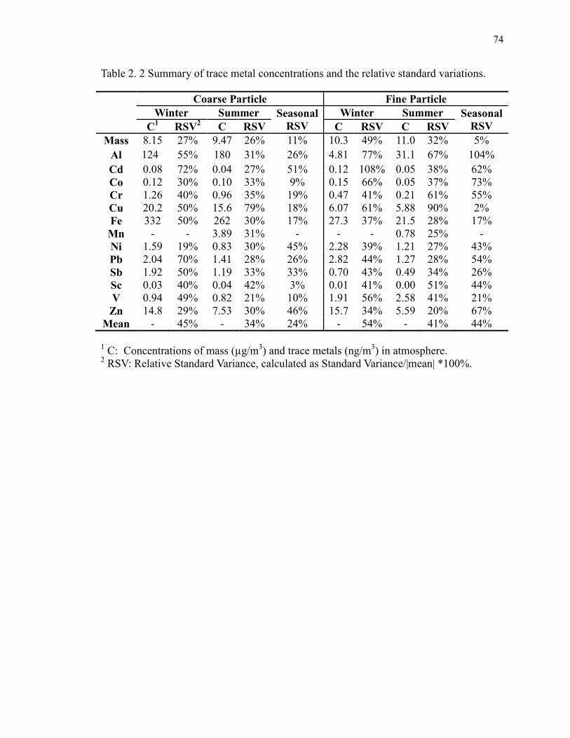
74
Table 2. 2 Summary of trace metal concentrations and the relative standard variations.
1 C: Concentrations of mass (µg/m
3) and trace metals (ng/m
3) in atmosphere.
2 RSV: Relative Standard Variance, calculated as Standard Variance/|mean| *100%.
Coarse Particle Fine Particle
Winter Summer Seasonal
RSV
Winter Summer Seasonal
RSV C1 RSV
2 C RSV C RSV C RSV
Mass 8.15 27% 9.47 26% 11% 10.3 49% 11.0 32% 5%
Al 124 55% 180 31% 26% 4.81 77% 31.1 67% 104%
Cd 0.08 72% 0.04 27% 51% 0.12 108% 0.05 38% 62%
Co 0.12 30% 0.10 33% 9% 0.15 66% 0.05 37% 73%
Cr 1.26 40% 0.96 35% 19% 0.47 41% 0.21 61% 55%
Cu 20.2 50% 15.6 79% 18% 6.07 61% 5.88 90% 2%
Fe 332 50% 262 30% 17% 27.3 37% 21.5 28% 17%
Mn - - 3.89 31% - - - 0.78 25% -
�i 1.59 19% 0.83 30% 45% 2.28 39% 1.21 27% 43%
Pb 2.04 70% 1.41 28% 26% 2.82 44% 1.27 28% 54%
Sb 1.92 50% 1.19 33% 33% 0.70 43% 0.49 34% 26%
Sc 0.03 40% 0.04 42% 3% 0.01 41% 0.00 51% 44%
V 0.94 49% 0.82 21% 10% 1.91 56% 2.58 41% 21%
Zn 14.8 29% 7.53 30% 46% 15.7 34% 5.59 20% 67%
Mean - 45% - 34% 24% - 54% - 41% 44%

75
Table 2. 3 Crustal enrichment factors of trace metals in fine, coarse and all particles.
Enrichment
Level
Trace
Metals
Fine Particle Coarse particle All particle
Winter Summer Winter Summer Winter Summer
Low
Fe 5.74 0.996 4.66 3.70 4.73 2.12
Sc 0.0427 1.22 0.71 1.55 0.67 1.04
Co 68.1 4.29 3.54 3.14 7.77 2.44
Mn - 1.77 - 3.15 - 1.98
Medium
Cr 85.5 17.4 18.4 19.0 22.7 13.2
Ni 305.2 39.5 9.78 5.01 29.1 9.99
V 156.3 47.0 4.80 4.51 14.7 11.1
High
Cu 1020 246 254 239 304 170.6
Cd 10600 778 443 187 1110 243
Sb 38700 526 7370 4570 9430 3360
Medium/
High
Pb 2090 190 90.5 65.6 222 69.7
Zn 2340 226 147 90.6 290 89.5

76
Table 2. 4 Similarity levels of size distributions in/between different seasons (Centroid
Linkage Method).
Concentrations Enrichment Factors
Winter1 Summer
1 Seasonal
2 Winter
1 Summer
1 Seasonal
2
Mass 81.8% 74.5% 98.2% - - -
Al 88.2% 86.8% 98.6% - - -
Cd 46.2% 83.1% 82.3% 84.5% 87.1% 93.7%
Cr 68.8% 72.7% 91.8% 67.4% 38.3% 91.0%
Cu 63.1% 86.9% 97.7% 67.4% 76.1% 81.3%
Co 75.7% 84.3% 70.8% 96.6% 92.7% 99.3%
Fe 91.6% 92.9% 97.6% 66.2% 77.6% 57.5%
Mn - 93.3% - - 53.9% -
�i 83.1% 87.7% 99.9% 98.7% 96.7% 99.5%
Pb 90.9% 60.3% 89.8% 91.1% 85.8% 97.0%
Sb 89.6% 86.3% 97.3% 93.3% 76.0% 89.8%
Sc 91.2% 86.3% 95.6% 44.6% 43.1% 15.5%
V 92.2% 98.8% 99.8% 98.7% 96.8% 99.3%
Zn 62.5% 64.1% 91.0% 93.1% 88.6% 94.4%
1 Variations in each season.
2 Seasonal variations of averaged patterns.

77
Table 2. 5 Size distributions of trace metals by cluster analysis.
Group Cluster Similarity Component
Winter Summer
Group I
C1 93.9% Al, Cr, Fe, Sc Al, Cr, Fe, Sc, Mn
C2 89.5% Cu, Sb Cu, Sb
C3 100% - Co
Group II
C4 100% Cd -
C5 92.4% Pb, Zn Cd, Pb, Zn
C6 93.1% Ni, V Ni, V, Co

78
Table 2. 6 Factor Analysis Result of trace metals concentrations.
Factor1 Factor2 Factor3 Communality
Cd 0.875 -0.093 0.306 0.867
Cr 0.605 0.739 -0.071 0.917
Cu 0.007 0.89 0.208 0.835
Co 0.04 0.106 0.969 0.951
Fe 0.823 0.426 0.039 0.861
�i 0.285 0.645 0.549 0.798
Pb 0.936 0.235 0.119 0.945
Sb 0.723 0.516 0.307 0.884
V 0.257 0.735 -0.336 0.719
Zn 0.377 -0.094 0.875 0.917
Variance 3.50 2.83 2.37 8.69
Var% 0.350 0.283 0.237 0.869

79
Table 2. 7 Identified Clusters of MOUDI sampling events and their dominant factors.
CLUSTER Dominant Factors MOUDI Sampling #
Winter Summer
C1 None 2 8, 9, 10, 11
C2 F2 1, 3, 4 7
C3 F3 5 -
C4 F1 6 -

80
Table 2. 8 Correlations between weather parameters and trace metal concentrations.
Coarse Particles Fine Particles
Item Mid
Dp Temp.
Wind
Speed Precip. Item
Mid
Dp Temp.
Wind
Speed Precip.
Mass 4.4 0.684
* -0.772 -0.69
Al
0.78 0.61
- - (0.02)
** (0.005) (0.019) (0.046)
Al 7.8 - -0.626
- 0.44 0.729
- -0.765
(0.039) (0.011) (0.006)
Cr 7.8 - -0.617
- 0.25 0.694
- -0.685
(0.043) (0.018) (0.02)
Ni
14 - 0.62
-
Pb
0.44 -0.617
- - (0.042) (0.043)
7.8 -0.632
- - 0.25 -0.608
- - (0.037) (0.047)
Pb
14 - -0.69
-
V
0.44 - -0.751 -0.661
(0.019) (0.008) (0.027)
7.8 - -0.759
- 0.25 - -0.724 -0.63
(0.007) (0.012) (0.038)
Sc
14 - -0.798
-
Zn
0.44 -0.699
- - (0.003) (0.017)
7.8 0.649 -0.714
- 0.25 -0.713
- 0.665
(0.031) (0.014) (0.014) (0.025)
4.4 0.713
- -
Sc
0.78 0.865
- -0.681
(0.014) (0.001) (0.021)
2.5 0.669
- - 0.44 0.919
- -0.731
(0.024) (<0.001) (0.011)
1.4 0.812
- - 0.25 0.945
- -0.645
(0.002) (<0.001) (0.032)
Co 2.5 - - 0.633
Co 0.44 -0.644
- 0.618
(0.037) (0.033) (0.043)
* Correlation factors.
** Significant levels.
81
Figure 2. 1 Map of sampling location.

82
dC
/dlo
g(d
Dp
) (µ
g/m
3)
Dp (µm)
Average
0.1 1 10 100
0
10
20
30
40
Winter
Summer
Summer
0
10
20
30
40#7
#8
#9
#10
#11
Winter
0
10
20
30
40#1
#2
#3
#4
#5
#6
Figure 2. 2 The mass size distribution of particles in winter and summer.

83
Group I
0.1 1 10 100
0.0
0.2
0.4
0.6
0.8
1.0
1.2
Cluster 1
Cluster 2
Cluster 3
Dp (µm)
Rel
ati
ve
dC
/dlo
g(d
Dp
)
Group II
0.1 1 10 100
Cluster 4
Cluster 5
Cluster 6
Figure 2. 3 The mass size distribution trace metals in two groups: (I) Coarse Particle
Accumulation and (II) Fine Particle Accumulation.

84
Rel
ati
ve d
C/d
log(d
Dp
)
Cluster 2
0.0
0.2
0.4
0.6
0.8
1.0Cu_w
Cu_S
Sb_W
Sb_S
Cluster 1
0.0
0.2
0.4
0.6
0.8
1.0Al_W
Al_S
Cr_W
Cr_S
Fe_W
Fe_S
Sc_W
Sc_S
Mn_S
Cluster 5 Cd_S
Pb_W
Pb_S
Zn_W
Zn- S
Cluster 4 Cd_W
Cluster 3
0.1 1 10 100
0.0
0.2
0.4
0.6
0.8
1.0 Co_S Cluster 6
0.1 1 10 100
�i_W
�i_S
V_W
V_S
Co_W
Dp (µm)
Figure 2. 4 The mass size distributions of the 6 identified clusters of trace metals in
atmosphere (In the figure labels, W means winter while S means summer).

85
Figure 2. 5 The EF size distributions of the trace metal in three different clusters: (a)
Cluster 1, (b) Cluster 2, (c) Cluster 3 and (d) Comparison of the average patterns of the
three clusters.

86
Figure 2. 6 Back-Trajectories of air mass using NOAA HYSPLIT Model with arriving
height 5 m and duration 48 hours: (a). Cluster 1 (Sampling set #9 as example), (b).
Cluster 2 (Sampling set #4 as example), (c). Cluster 3 (Sampling set #5 as example), (d).
Cluster 4 (Sampling set #6 as example). For each sampling period (3- 4days), a total of
24 Back-Trajectories were calculated with same interval (3-4 hours).

87
Chapter 3 . Relationships among the Springtime Ground-level
NOx, O3 and NO3 in the Vicinity of Highways in the
US East Coast*
* This work is in press by Atmospheric Pollution Research (APR) and is scheduled to be
published in the third issue in 2011.

88
Abstract
To characterize the relationships among the springtime NOx (NO + NO2), O3 and
NO3 (defined as the combination of gaseous nitric acid, HNO3, and aerosol nitrate, NO3-)
concentrations in the ambient air of the vicinity of highways, an intensive sampling was
carried out in spring 2007 at Lyndhurst, NJ in the US East Coast. Ambient concentrations
of O3 and NOx were measured by O3 and NOx analyzers, while NO3 was collected using a
ChemComb cartridge and determined by ion chromatography. Significant variations in
O3 concentrations were observed diurnally as well as between weekdays and weekends,
with higher concentrations occurring during the daytime and on weekends. The 24-h
diurnal variations of O3 and NOx could be divided into four periods: (1) morning NOx
peak, (2) mid-day O3 formation, (3) afternoon NOx accumulation and (4) nighttime
balancing. Daily averaged relative humidity and wind speed were the two important
weather parameters affecting O3 levels and the corresponding photochemical reactions,
and daily maximum temperature was positively correlated to maximum O3. Via
photochemical reactions and emission-diffusion balance, NOx showed primarily negative
influences on the daily O3 variations with decayed exponential correlations, in particular
during nighttime and weekdays, indicating a possible VOC-sensitive characteristic of the
study area. A negative correlation between NO3- and O3 concentrations was found while
no obvious influences of HNO3 on O3 was observed. Results by a multi-regression model
involving three parameters (NO2/OX ratio, NO2 and HNO3) reveal that the NO2/OX ratio
is an important parameter controlling the ground O3 level in the study area.
Key words: O3, NOx, NO3, influences, variations.

89
3.1. Introduction
Ozone (O3) and nitrogen oxides (NOx = NO + NO2) are two of the six principle
pollutants in the National Ambient Air Quality Standards (NAAQS) in the US since 1990,
as at high concentrations they could induce serious adverse effects on human health and
the environment (Lee et al., 1996; WHO, 2000; Kampa and Castanas, 2007). Besides, the
photochemical reactions between NOx and O3 play key roles in altering the atmospheric
oxidation/reduction capacity and in transferring nitrogen from the atmosphere to the
aquatic ecosystems that affect many biogeochemical processes.
In the near-ground atmosphere, NOx and O3 are connected via photochemical
inter-conversions as shown below (Seinfeld and Pandis, 2006):
NO2 + hν NO + O R1
O + O2 + M O3 + M R2
O3 + NO NO2 + O2 R3
These reactions may change the ratios of NO/NO2, NO2/NOx, and NO2/O3, but
they cannot change the NOx or OX (= NO2 + O3) level, an indicator of oxidizing level of
the ambient atmosphere (Clapp and Jenkin, 2001). However, certain volatile organic
compounds (VOC) could influence NOx-O3 photochemical reactions (Seinfeld and
Pandis, 2006; Wei et al., 2007). With the existence of OH radicals, VOC can oxidize NO
to NO2 and thus promote O3 production during daytime (Atkinson, 2000; Seinfeld and
Pandis, 2006).
Ground level O3 comes from two major sources: regional background O3
primarily from the influx of O3 from the stratosphere and in situ local O3 production
mainly via photochemical reactions (shown in R1-R3) involving many precursors, such

90
as NOx and VOC, emitted from a variety of anthropogenic and nature sources (Clapp and
Jenkin, 2001; Vingarzan, 2004; Cofala et al., 2007; The Royal Society, 2008; and
Rappenglück et al., 2008). Combustion processes are the major sources of NOx in the air,
especially vehicle emissions in high traffic areas. In the eastern United States, the vehicle
emission source contributed more than half of the total NOx emissions (Butler et al., 2005)
that could significantly affect the ambient O3 levels, and this emission source has showed
an increasing trend since the 1990s (Parrish, 2006). In such high NOx emission regions,
O3 is often depleted locally/regionally by titration. OX is therefore a more stable entity to
study, as it is an indication of the potential for renewed ozone production downwind of
the sources. However, the cycling between NO and NO2 is rapid and NO2 could be lost
via dry deposition and chemistry, these processes may complicate the observed NOx and
O3 in the ambient air, affecting the ratio of NO2/NOx.
On the other hand, the production of Nitrate (NO3), defined in this study as the
combination of gaseous nitric acid (HNO3) and aerosol nitrate (NO3-), is also related to
the ground-level O3. In daytime, HNO3 could be directly produced via R4 when the
VOC/NO2 ratio is small (on average < 5.5 in urban areas). In nighttime, different HNO3
production mechanisms exist as shown in R5-R7 (Seinfeld and Pandis, 2006), and NO3-
could be produced via acid-alkali reactions of HNO3.
NO2 + OH + M HNO3 + M R4
O3 + NO2 NO3 + O2 R5
NO3 + NO2 + M N2O5 + M R6
N2O5 (g) + H2O (l) 2 HNO3(aq) R7
Although many studies have been carried out on the photochemical characteristics

91
of NOx and O3, in particular in the US west coast (CARB, 2003; Qin et al., 2004a and
2004b; Yarwood et al., 2008; Alvarez et al., 2008), few such studies have been conducted
recently in the US east coast, especially in high-traffic areas. Besides, while NOx was
known as an O3 precursor, the role of NO3 on the variations of O3 levels was seldom
studied. In order to characterize NOx and O3 in a typical high-traffic area in the US east
coast and to explore the influences of both NOx and NO3 on O3 variations, we carried out
an intensive sampling campaign at Lyndhurst in northeast New Jersey (NJ), which is
surrounded by many highways. The field measurements took place in spring 2007,
because the spring is a transitional season from cold to warm weather when the O3
concentrations are relatively higher (Monks, 2000; Lehman et al., 2004; Kaiser et al.,
2007) and the exceedances of the NAQQS standard for O3 have happened often in NJ
(http://www.state.nj.us/dep/). The results from this study will fill the data gap for urban
ground level O3, NOx, and NO3 in the region, help better understand the mechanisms
controlling O3 concentrations and variations, and provide useful information for
modeling and prediction of O3 concentrations.
3.2. Method
3.2.1. Sampling
In spring 2007 from Feb. 22nd
to May 21st, real-time monitoring of NOx and O3
was conducted at the Meadowlands site housed at Meadowlands Environmental Research
Institute in Lyndhurst, NJ (41ºN, 74ºW), ~ 1 km away from major high-ways (Fig. 3.1).
Measurements of NO and NO2 were made continuously with a 42i NOx Analyzer
(Thermo Electron Corporation, Franklin, MA). A model 49i UV photometric ozone
analyzer (Thermo Electron Corporation, Franklin, MA) was used for the continuous

92
measurement of O3. The air detected was pumped through two monitoring instruments
via two lengths of separated plastic tubing with inlets installed on the roof of a building,
~8 m above the ground. The instruments have 1-minute resolution, with detectable limits
of 0.40ppb for NOx and 0.50ppb for O3. During the measurement period, the two
analyzers were calibrated biweekly which resulted in certain gaps in data collection.
Sampling of the gaseous HNO3 and aerosol NO3- was conducted daily using a
ChemComb Cartridge (Model 3500, Thermo Scientific), with a flow rate maintained at
15L/Min. Nylon filters (Pall Corporation, 1.0µm pore size) were used for HNO3
collection while NO3- was collected on Teflon filters (Pall Corporation, 1.0µm pore size).
The sampling inlet was set at the same place where the inlets for NOx and O3 were
installed. All samples were kept in refrigerator until analysis.
To assist data interpretation, certain meteorological parameters including air
Temperature (T), Solar Radiation (SR), Rainfall, Relative Humidity (RH) and Wind
Speed (WS) were also collected in the study area. The time interval for weather data
retrievals was 15 minutes.
3.2.2. Chemical determinations
Determinations of NOx were made online by detecting the chemiluminescence in
the range of 600nm to 3000nm generated by NO2 radicals produced from reactions
between O3 and NO, based on the principle that NO and O3 react to create luminescence
with an intensity linearly proportional to the NO concentration. Determination of O3 was
carried out by the UV photometric method, since O3 molecules absorb UV radiation at a
wavelength of 254nm and the relationship between the absorbance of the UV light and
the ozone concentration follows the Lambert-Beer law.

93
Gaseous HNO3 and aerosol NO3- were measured using IC (ICS-2000, Dionex) in
the Atmosphere Chemistry Lab of Rutgers University at Newark based on the procedures
of Lee et al (1994) and Zhao and Gao (2008). Sample filters were ultrasonically extracted
in DI water for 30 minutes, and then the solutions were filtered with a PTFE syringe filter
(Fisher brand, 0.45 µm). Sample solutions were injected into the IC via automated
sampler (AS40, Dionex) using 0.5ml vials. An AS11 analytical column (2_250mm2,
Dionex), KOH eluent generator cartridge (EGC II KOH, Dionex) and 25µl sample loop
were employed for the determinations. The detection limit of the method is below
0.01ppm, and the precision of the analysis is ~ 1%.
3.2.3. Data processing
The 1-minute interval data was integrated to obtain hourly averaged data by
averaging all qualified data in one hour using homogeneity testing. The hourly averaged
data in each day were then divided into two parts: daytime (7:00 to 19:00) and nighttime
(19:01 to 6:59), considering the average solar radiation changes of a day in the spring in
NJ. To better interpret the data, Pearson Correlation, Factor Analysis, Custer Analysis,
and Multi-regression Simulation Modeling were used in this study, and all the statistical
analyses in the study were carried out using MiniTab 14 (Minitab Statistical Software).
3.3. Results and Discussions
3.3.1. Overall Concentrations and 24-hour Variations Characteristics
3.3.1.1. Concentrations
The average concentrations of ground level NO, NO2 and O3 in the study area
were 13.8ppb, 21.3ppb and 24.0ppb, respectively, satisfying NAAQS’s primary and
secondary standards requirement (Table 3.1). Different from other locations (Qin et al.,

94
2004b; Mazzeo et al., 2005), the NO2 concentrations at the Meadowland site in this study
were high and even greatly exceeded the NO concentrations, indicating a higher
oxidizing level of the environment in this region. High concentrations of NO2 were also
observed in another two sites in NJ at Chester and Elizabeth listed in Table 3.1, although
compared with these two sites, the NOx concentrations at the Meadowlands site were
moderate. The concentrations of HNO3 and NO3- were close to each other, averaging
1.24µg/m3 and 1.80µg/m
3, respectively. Compared with other sites (Danalatos and Glavas,
1999; Bari et al., 2003; Lin et al., 2006), the HNO3 concentration was low while the level
of NO3- was found comparable.
During the study period, the daily averaged concentrations of O3 and HNO3
showed less variation, compared with those of NOx and NO3- (Fig. 3.3). The
concentrations of O3 were limited to a range from ~ 7ppb to ~ 40ppb with a roughly
normal distribution, while the concentrations of NOx, especially NO, fluctuated over a
larger range and were biased away from normal distributions at high concentrations.
Similar situations happened for aerosol NO3-. Both NOx and NO3
- showed more extreme
high values, and this may reflect the existence of irregular high emissions of NOx in the
study region.
As shown in Fig. 3.4, the weekly averaged concentrations of O3 slightly increased
during the study period, while those of NOx and NO3 decreased. Besides the influences of
weather changes, such as temperature, solar radiation etc, the emission-diffusion balance
of NOx and regional O3 could also be a reason for the variations in the time series,
considering the fact that NOx showed maximum values in late autumn and winter (Tu et
al., 2007), while O3 regional background could reach its maximum in spring and summer

95
(Monks, 2000; Lehman et al., 2004; Kaiser et al., 2007).
3.3.1.2. 24-hour Variations
Diurnal variations of NO, NO2 and O3 were observed in this study, especially for
O3. The concentrations of NO and O3 were higher in daytime while opposite trends exist
for NO2 and NOx (Table 3.2), attributed to the photochemical reactions of NOx and O3
and the balance between emissions (natural and anthropogenic) and mixing processes of
both horizontal dispersions and vertical convections. During daytime, NO2 is oxidized by
hydroxyl radical (OH) and produced gaseous HNO3; while in the nighttime, O3 could
oxidize NO to NO2 without solar radiation. The further oxidation of NO2 by O3 formed
nitrate radical NO3. In addition, the relatively low air temperature near the ground at
night could prevent the vertical dispersion of NOx, contributing to its accumulation and
resulting in higher night-time concentrations.
The 24-h temporal variations of NOx and O3 can be divided into four periods (Fig.
3.5). The variations in each period can be explained by photochemical processes and the
emissions-dilution balance of NOx and O3. In the first period (3:00-7:00), the NOx
concentrations at the study site increased suddenly, reflecting increased emissions of
motor vehicles during the morning rush hours and from industrial activities. The newly
emitted NO could react with O3 without solar radiation, producing more NO2 and
reducing O3 concentrations. During the second period (7:00-15:00), the solar radiation
increased greatly and the photochemical processes that produce O3 dominated, especially
at the beginning of this period. Oxygen atoms produced in the photolysis of NO2 could
react with O2 to produce O3 as described by R1 and R2. Around 15:00, O3 showed peak
values when NOx had the lowest concentrations. In this period, the NOx accumulations

96
were not significant because of the high NOx photochemical consumption and increased
air mass dilution as the height of the boundary layer increases. The boundary layer height
should reach a maximum sometimes in the afternoon, plus additional venting of the
boundary layer by convection.
Then, in the 3rd
period (15:00-20:00), the photochemical production of O3
decreased while the NO2 level increased. The reduced O3 level could be explained mainly
by the decrease of SR, which then would lower the level of photochemical production.
NOx could accumulate again because of afternoon-hour high-traffic emissions in the
period. However, due to the high dilution level similar to the 2nd
period, the 3rd
period
NOx could not accumulate as high as in the 1st period. In the 4
th period (20:00-3:00), the
NOx and O3 balance arrived quickly and was maintained; as there was no solar radiation
and both source emissions and dilution effects decreased significantly.
3.3.2. Weekday/Weekend and Diurnal Variation
Both NOx and O3 concentrations showed a difference between weekdays and
weekends. Compared with weekends, the concentrations of NO, NO2 and NOx on
weekdays were higher while the O3 concentration was lower (Table 3.2), consistent with
the results from studies in other locations (Cleveland et al., 1974; Marr and Harley, 2002;
Qin et al., 2004a). In addition, similar to the results of Pudasainee et al. (2006), the
concentrations of O3 for weekends were ~13.4% higher than weekdays in this area.
However, the mechanisms for the weekday/weekend variations of NOx and O3 are not
clear. The California Air Resource Board (CARB) (2004) proposed a hypothesis that
VOCs become sensitive to O3 formation when NOx emission decreases on weekends
(Altshuler et al., 1995; Blanchard and Fairley, 2001; a et al., 2004). The weekly pattern of

97
traffic flows was also thought to affect the weekday/weekend variations of NOx and O3
(Shutters and Balling, Jr., 2006). It is possible that the study site is under a VOC-sensitive
environment, based on the fact that the concentrations of NOx and O3 are negatively
correlated (which will be discussed later) and the fact that NOx concentrations decreased
on weekends.
Diurnal variations of NOx and O3 were also observed in this study, especially for
O3. The concentrations of NO and O3 were higher in daytime while opposite trends exist
for NOx (Table 3.2), attributed to the photochemical reactions of NOx and O3. During
daytime, NO2 is oxidized by hydroxyl radical (OH) and produced gaseous HNO3; while
in the nighttime, O3 could oxidize NO to NO2 without solar radiation. The further
oxidation of NO2 by O3 formed nitrate radical NO3. In addition, the relatively low air
temperature near the ground at night could prevent the vertical dispersion of NOx,
contributing to its accumulation and resulting in higher night-time concentrations.
Fig. 3.6 shows that the 24-h diurnal variation patterns of NOx and O3 were also
different between weekdays and weekends. The weekday morning peaks of NOx and O3
concentrations were higher than those over the weekends, indicating higher traffic
emissions during rush hours. On weekends, in the 1st period, NOx showed less
accumulation due to less traffic and industries emissions, while O3 concentrations were
higher. During the second period, the O3 accumulation continued and NOx started to
decrease. The 3rd
period lasted much longer in weekends as the O3 concentrations were
higher while NOx inputs were lower. The 4th
period was shorter with less variation in the
concentrations compared with those for weekdays; as a result of rapid chemistry and
advection out of the area, the lower values observed at daytime in weekends does not

98
affect night time NOx levels that much. However, on weekends, NOx showed an increase
after 24:00 to 3:00 of the following day, probably due to increased traffic volumes at late
night on weekends compared with weekdays.
3.3.3. Weather Influences on Concentrations
3.3.3.1. Daily Concentrations
The daily averaged meteorological parameters (Temperature (T), Solar radiation
(SR), relative Humidity (RH) and Wind speed (WS) were found to influence the
concentrations of NOx, O3 and NO3 (Table 3.3), consistent with previous studies (Mazzeo
et al., 2005; Nevers, 2000; Tu et al., 2007). However, in contrast to the conclusion of
previous studies (O'Connor et al., 2005; Pudasainee et al., 2006; Castell et al., 2007), the
daily averaged T did not show much influences on O3 concentrations at this location.
This suggests that the correlation between pollution levels and meteorology is weaker
during spring, compared with summer (O'Connor, 2005). In addition, the averaged daily
data used in the calculations could further reduce the correlation, as the recalculated
correlation between daily maximum T and O3 showed significant positive correlation (p
<0.01). On the other hand, the proximity to anthropogenic emissions may also mask
correlation between ozone and temperature, according to a recent study by Castell (2007)
who found in Castellon (Spain) on the Western Mediterranean area, the correlations
between ozone and meteorological variables at inland stations (away from anthropogenic
emissions) are better than those at coastal stations (close to human emissions). T and SR
were found to influence NO3 only, and the higher T and SR would more probably induce
a higher HNO3 level and lower NO3- level, respectively.
RH and WS were found to be of more importance in this study compared with

99
other weather parameters. In general, the results showed that when RH increased, NOx
and NO3- increased but O3 decreased, indicating that high RH may retard the O3
production to some extent, while the underlying mechanism is not clear due to limited
data collection during this study. Possible mechanisms driving this phenomenon should
be explored through future investigations. High WS could lower NOx and NO3-
concentrations due to the dilution effect. However, the positive correlations between WS
and O3 were found, and this could be caused by the transport of high O3 air into this area
from upwind pollution sources. The results relating the effects of weather conditions
certainly reveal the complexity of the observed NOx and O3 levels affected by many
processes happening both instantaneously and over time.
3.3.3.2. Diurnal Variations
Primarily, the 24-h diurnal variation patterns of NOx and O3 in different weather
conditions were similar, as shown in Fig. 3.7. To characterize the potential weather
influences on the 24-h temporal variations of these species, the study period was
categorized into three groups using cluster analysis with respect to the values of SR, RH
and precipitation,: clear days, cloudy days and rainy days, with each counting about 1/3
of the entire study period (Table 3.4). In all weather conditions, the O3 peaks appeared in
the period of 14:00 to 16:00, and the maximum O3 concentration (>40 ppb) during that
period was associated with clear days (Fig. 3.7a), reflecting the strong influence of SR on
the in situ photochemical accumulation of O3 and enhanced mixing from aloft.
Coinciding with high traffic hours, the NOx concentration peaks appeared in early
morning and evening, indicating the influence of high vehicle emissions on NOx levels
during those periods of time. The NOx peaks were more obvious in the morning than

100
those in the afternoon, strengthened by the atmospheric inversion developed over the
night hours. Compared with cloudy and rainy days, the NOx level was lower and O3
accumulated to a higher level during clear days, possibly due to photochemical reactions
that were more intensive in clear days.
3.3.4. Correlations between NOx and O3
Fig. 3.8 shows that the concentrations of NOx and O3 were negatively correlated
exponentially throughout the study period, suggesting possible VOC-sensitive
characteristics of the study site, as described in Seinfeld and Pandis (2006). While the
instantaneous photochemical reaction dynamics during the day affect the production rate
of O3, the correlations between averaged NOx and O3 concentrations over certain period
of time reflect the mixed effects of chemical reactions, transport patterns, atmospheric
dispersion and etc. The nature of the negative correlations between NOx and O3 indicates
that the study site is not NOx sensitive but possibly VOC sensitive, assuming that the
higher O3 levels appear when the VOC concentrations increase. A high level of NOx
would consume more OH radicals through HNO3-forming reactions and thus lower the
oxidizing ability of VOC and NO2, which are the two precursors of O3 (Sillman and He,
2002; Seinfeld and Pandis, 2006; Cofala et al., 2007). The fact that the NO2/NOx ratio
decreased greatly as NOx increased that could be newly emitted could also support the
VOC-sensitive nature of the region (Fig. 3.2). Nevertheless, VOC may also be emitted by
traffic, and more detailed relationships among NOx, VOC and O3 in this area need to be
explored through future studies.
Compared with those for nighttime and weekdays, the daytime and weekend NOx
levels showed less negative influence on O3 concentrations (Fig. 3.8). While O3

101
consumption through reactions with NOx dominated during nighttime, NOx could either
produce O3 or consume O3 production during the daytime: on one hand, when VOC was
sufficient, NO2 could react with O2 to produce O3. On the other hand, the newly produced
O3 would oxidize NO to NO2 and thus lower the O3 level when VOC was limited.
Therefore the negative influences of NOx on O3 were more significant during the
nighttime. The lower negative effects of NOx on O3 during weekends could be attributed
to two reasons: (1) NOx may not accumulate much, and (2) the effect of VOC may be
more active during weekends (CARB, 2004); both lead to increased O3 production.
3.3.5. Correlations between NOx and OX
The level of OX, an oxidizing level indicator of the NOx- O3 regime, could be
increased in two ways: (1) the net increase of NO2 through NOx emissions and then
oxidization of NO to NO2 by radical species such as RO2 (where R is a hydrogen atom or
carbon containing fragment), OH etc. (Atkinson, 2000; Seinfeld and Pandis, 2006), and
(2) the net increase of O3 via regional background input. The direct input of NO2 is
mainly controlled by net NOx emission and the original NO2/NOx ratio, which could be
approximated by the lower end ratios while NOx increases (Carslaw, 2005; Seinfeld and
Pandis, 2006). As shown in Fig. 3.8, the NO2/NOx ratios in the study area varied and
finally reached balance at ~ 20% when NOx increased. This is consistent with the
conclusion of an increasing NO2/NOx ratio obtained at a roadside in London, reaching to
~ 17% (Carslaw, 2005), and the increase in the NO2/NOx emissions ratio from road traffic
in recent years is believed to have a significant effect on recent trends in roadside NO2
concentrations in the area. The feature in NO2/NOx ratio in European emissions is
primarily driven by light duty diesel vehicles after treatment technologies (Alvarez et al.,

102
2008). Thus the contribution of NOx to OX via NO2 input found in this study could be
treated as 20% which might indirectly represent the current emission situations in these
regions, although the detailed explanations still need to be explored further. The other OX
could be explained by regional O3 input and the radical reactions producing net OX.
The net effect of photochemical reactions between NOx and O3 was the
consumption of O3, especially in daytime and weekends as shown in Fig. 3.8. As stated
earlier, the ground level O3 is mainly composed of background O3 and local production of
O3. Because NOx plays a critical role in the local O3 production as shown in equation R1-
R3, the background O3 can be approximated from the total O3 concentrations in the
scenario that NOx does not existed. The regional O3 background level thus could be
interpreted as the interceptions of the OX-NOx linear relation in Fig. 3.9 (Clapp and
Jenkin, 2001). The derived background O3 concentration was higher than the daily
averaged total O3 (Table 3.1) in the study area. It suggests that the net effect of NOx
related local processes is the consumption of O3. Thus in the study area, the O3
consumption, which mainly happened at night, exceeded the O3 production via
photochemical reactions involving VOC and NOx during the day.
The OX level of the study area was controlled mainly by the net NOx emissions,
while photochemical reactions of NOx and O3 contributed much less to OX. As shown in
Fig. 3.9, the slopes of the OX-NOx linear relations were ~0.20, close to the original
NO2/NOx ratio in the study area shown in Fig. 3.2. Considering the fact that the quick
cycling between NO and NO2 would not change the ratio of OX/NOx as shown in R1–R3,
this result indicates the dominant influence of NOx accumulations on OX. For weekdays,
the slopes were smaller than 0.20, indicating the NO2 consumption exceeded NO2

103
formation, especially in daytime. However, with the higher NOx levels, the NO3
concentrations for weekdays were lower (Table 3.2), suggesting that other NO2
consumption mechanisms may also exist in addition to the mechanisms shown in R5-R7.
For weekends, the slopes were higher than 0.20 (Fig. 3.9), indicating that NO2
oxidizations were significant and O3 net production may exist. This is consistent with the
higher O3 level during weekends and daytime shown in Table 3.2.
3.3.6. Relationships between NO3 and O3
Preliminary results from this study show that NO3- was involved in the O3
variations, and a higher NO3- level was primarily associated with a lower O3 level. As
shown in Table 3.3, the daily averaged concentrations of NO3- showed significantly
negative correlation with those of O3, attributed to R5-R7, while no correlations between
HNO3 and O3 were found. Strong positive correlations between NO3- and NOx were also
observed, which was consistent with the negative relationships between NO3- and O3. In
addition, in high NOx environments, O3 is depleted locally by titration, while NO3- could
be buildup, which also supports the negative NO3--O3 correlation. Through factor
analysis (PCA method with Varimax Rotation), the concentrations of NOx and O3, NO3-
and O3, were grouped to factor 1 and factor 2, respectively, with HNO3 alone serving as
factor 3 (Table 3.5). These results suggest the significant correlations between NO3- and
O3 and no correlations for HNO3. However, the underlying mechanisms for their
relationships are not clear and should be explored through future studies.
3.3.7. Multi-Regression analysis of the NOx-O3-NO3 system
Multi-regression methods were used to explore the ground-level O3 concentration
variations with respect to the influences of daily averaged level of NO2/OX ratio, NO2

104
and HNO3 observed in this study. The results show that the NO2/OX ratio was the most
influential factor on the O3 level, suggested by its large coefficients and the average
NO2/OX (Table 3.6). The NO2 concentration, which was found to have negative influence
on the O3 level as discussed in previous sections, functioned as the compensatory
correction to the influences of the NO2/OX ratio on O3. HNO3, which was less important,
is considered as a conditional explaining factor. These three factors selected could
account for a total of 85.7% of the variations of O3 for the entire study period.
The NO2/OX ratio became a more powerful factor when the NOx level increased.
For better simulation, the whole investigation period was divided into 4 clusters, using
cluster analysis (Ward's method) with the concentrations of NOx, NO3 and O3 (Table 3.6).
From cluster 1 to 4, the NOx, NO3-, NO2/OX increased while O3, NO2/NOx, HNO3/NO3
decreased. The results from these multi-regression functions (Table 3.6) of each cluster
can explain the O3 variations, and the most important factor was NO2/OX. However, the
weight of each factor changed greatly. When the NOx level was low, the NO2
concentrations played a more important role, and such influence was reduced greatly
when NOx levels increased. HNO3 was only used to explain the O3 variations when NOx
levels were either low or high.
3.4. Conclusions
Results from this study on the influences of NOx and NO3 on O3 levels carried out
during the springtime of 2007 lead to the following conclusions:
The study area was a relatively highly oxidizing level environment, with the
NO2/NOx ratio higher than many other regions. Ground level O3 concentrations showed
both weekday/weekend and diurnal variations, with high concentrations on weekends

105
possibly due to the increased VOC sensitivity and decreased NOx emissions, and in
daytime due to the photochemical production of O3 accompanied by lower O3
consumption. In the time series, the O3 concentrations generally increased from the
beginning to the end of the study period.
Due to the variations of photochemical processes and emissions-diffusion
balancing, the 24-h temporal variations patterns of NOx and O3 could be divided into four
periods: (1) morning NOx peak, (2) O3 formation, (3) afternoon NOx accumulation, and
(4) night balancing. Certain meteorological parameters, in particular relative humidity
and wind speed, played more important roles in O3 concentration variations and the
photochemical reactions of NOx and O3. Different 24-h temporal variations of NOx and
O3 were observed during different weather conditions. The daily maximum temperature
showed positive correlation to the daily maximum O3 level.
The net effect of NOx on O3 concentrations was negative with a decayed
exponential correlation, especially in nighttime and weekdays, indicating a possible
VOC-sensitive characteristic of the study area as observed y previous studies. The OX
levels were mostly controlled by NOx emissions and were less influenced by
photochemical reactions. The photochemical reactions of NOx and O3 led to a net O3
consumption.
Significant negative correlations between NO3- and O3 were found during this
study, indicating either a high connection between NOx and NO3- or an O3 retarding
characteristic for NO3-. HNO3 was not found to be related to the NOx-O3 system, with no
influence on the O3 level.
NO2/OX ratio, NO2 and HNO3 could be used to explain the O3 concentration

106
variations for about 85.7% of the O3 variations as shown in the whole study period. The
NO2/OX ratio was the most important factor in controlling O3 levels, and this influence
increased when NOx concentrations increased.
Acknowledgement
This work was primarily supported by Meadowlands Environmental Research
Institute of the New Jersey Commission. Additional support was provided by a New
Faculty Start-up Fund to YG at Rutgers University. We thank Yunliang Zhao, Kyung Hwa
Jung, and Christopher Thuman for sampling assistances and data collation.

107
3.5. References
Altshuler, S.L., Arcado, T.D., Lawson, D.R., 1995. Weekday vs. weekend ambient ozone
concentrations: discussion and hypotheses with focus on northern California.
Journal of the Air and Waste Management Association 45, 967–972.
Alvarez, R., Weilenmann, M., Favez J., 2008. Evidence of increased mass fraction of
NO2 within real-world NOx emissions of modern light vehicles — derived from a
reliable online measuring method. Atmospheric Environment 42, 4699-4707.
Arnold, J.R., Luke, W. T., 2007. Nitric acid and the origin and size segregation of aerosol
nitrate aloft during BRACE 2002. Atmospheric Environment 41, 4227–4241.
Atkinson, R., 2000. Atmospheric chemistry of VOCs and NOx. Atmospheric
Environment 34, 2063–2101.
Bari, A., Ferraro, V., Wilson, L.R., Luttinger, D., Husain, L., 2003. Measurements of
gaseous HONO, HNO3, SO2, HCl, NH3, particulate sulfate and PM2.5 in New York.
Atmospheric Environment 37, 2825 – 2835.
Blanchard, C.L., Fairley, D., 2001. Spatial mapping of VOC and NOx limitation of ozone
formation in central California. Atmospheric Environment 35, 3861–3873.
Butler, J. T., Likens, E. G., Vermeylen, M. F., Stunder, J.B. B., 2005. The impact of
changing nitrogen oxide emissions on wet and dry nitrogen deposition in the
northeastern USA. Atmospheric Environment 39, 4851-4862.
CARB, 2003. The ozone weekend effect in California. Staff Report, The Planning and
Technical Support Division, The Research Division, California Air Resources
Board, Sacramento, CA, 30 May. 37, 4205–4215.
Carslaw, D. C., 2005. Evidence of an increasing NO2/NOx emissions ratio from road

108
traffic emissions. Atmospheric Environment 39, 4793–4802.
Castell, N., Mantilla, E., Millan, M.M., 2008. Analysis of tropospheric ozone
concentration on a western mediterranean site: Castellon (Spain), Environmental
Monitoring and Assessment 136 (1), 3-11.
Clapp, L.J., and Jenkin, M.E., 2001. Analysis of relationship between ambient levels of
O3, NO2 and NO as a function of NOx in the UK. Atmospheric Environment 35,
6391-6405.
Cleveland, W.S., Graedel, T.E., Kleiner, B., Warner, K.L., 1974. Sunday and workday
variations in photochemical air pollutants in New Jersey and New York. Science
186, 1037–1038.
Cofala, J., Amann M., Klimont, Z., Kupiainen, K., Hoglund- Isaksson L., 2007. Scenarios
of global anthropogenic emissions of air pollutants and methane until 2030.
Atmospheric Environment 41, 8486–8499.
Danalatos, D., Glavas, P., 1999. Gas phase nitric acid, ammonias and related particulate
matter at a Mediterranean coastal site, Patra, Greece. Atmospheric Environment 33,
3417–3425.
Gaffney, J. S., Marley, N. A., Drayton, P. J., Doskey, P. V., Kotamarthi, V. R.,
Cunningham, M. M., 5 Baird, J. C., Dintaman, J., and Hart, H. L., 2002. Field
observations of regional and urban impacts of NO2, ozone, UV-B and nitrate radical
production rates in the Phoenix air basin, Atmospheric Environment 36, 825–833,
2002.
Kaiser, A., Scheifinger, H., Spangl, W., Weiss, A., Gilge, S., Fricke, W., Ries, L., Cemas,
D., Jesenovec, B., 2007. Transport of nitrogen oxides, carbon monoxide and ozone

109
to the Alpine Global Atmosphere Watch stations Jungfraujoch (Switzerland),
Zugspitze and Hohenpeissenberg (Germany), Sonnblick (Austria) and Mt. Krvavec
(Slovenia). Atmospheric Environment 41, 9273 - 9287.
Kampa, M., Castanas, E., 2007. Human health effects of air pollution. Environmental
Pollution 151, 362-367.
Lee, D.S., Holland, M.K., Falla, N., 1996. The potential impact of ozone on materials in
the UK. Atmospheric Environment 30, 1053–1065.
Lee, G.W., J.T. Merrill, and B.J. Huebert, Variation of free tropospheric total nitrate at
Mauna Loa Observatory, Journal of Geophysical Research 99, 12,821-12,831, 1994.
Lee, H.S., Wadden, R.A., Sche!, P.A., 1993. Measurement and evaluation of acid air
pollutants in Chicago using an annular denuder system. Atmospheric Environment
27A, 543-553.
Lehman, J., Swinton, K., Bortnick, S., Hamilton, C., Baldridge, E., Eder B., Cox, B.,
2004. Spatio-temporal characterization of tropospheric ozone across the eastern
United States, Atmospheric Environment 38, 4357–4369.
Lin, Y., Cheng, M., Ting, W., Yeh, W., 2006. Characteristics of gaseous HNO2, HNO3,
NH3 and particulate ammonium nitrate in an urban city of Central Taiwan.
Atmospheric Environment 40, 4725–4733.
Marr, L.C. and Harley, R.A., 2002. Spectral analysis of weekday–weekend differences in
ambient ozone, nitrogen oxide, and non-methane hydrocarbon time series in
California, Atmospheric Enviroment 36, 2327–2335.
Mazzeo, A.N., Venegas, E.L., Choren, H., 2005. Analysis of NO, NO2, O3 and NOx
concentrations measured at a green area of Buenos Aires City during wintertime.

110
Atmospheric Environment 39, 3055-3068.
Monks, P.S., 2000. A review of the observations and origins of the spring ozone
maximum. Atmospheric Environment 34, 3545–3561.
Nevers, N.D., 2000. Air Pollution Control Engineering, second ed. McGraw-Hill
Companies, Inc., New York, 571–573.
O'Connor, J.R., Roelle, P.A., Aneja, V.P., 2005. An ozone climatology: relationship
between meteorology and ozone in the southeast United States. International
Journal of Environment and Pollution 23 (2), 123-139.
Parrish, D.D., 2006. Critical evaluation of US on-road vehicle emission inventories,
Atmospheric Environment 40, 2288–2300.
Pudasainee, D., Sapkota, B., Shretha, L. M., Kaga A,, Konda A,, Inoue Y., 2006. Ground
level ozone concentrations and its association with NOx and meteorological
parameters in Kathmandu Valley, Nepal. Atmospheric Environment 40, 8081-8087.
Qin, Y., Tonnesen, G. S., Wang, Z., 2004a. Weekend/weekday differences of ozone, NOx,
CO, VOCs, PM10 and the light scatter during ozone season in southern California.
Atmospheric Environment 38, 3069-3087.
Qin, Y., Tonnesen, G.S., Wang, Z., 2004b. One hour and eight hour average ozone in
California south coast Air Basin: trends in peak values and sensitivity to precursors.
Atmospheric Environment 38, 2197–2207.
Rappenglück B., Perna R., Zhong S., Morris G.A., 2008. An Analysis of the Vertical
Structure of the Atmosphere and the Upper-Level Meteorology and their Impact on
Surface Ozone Levels in Houston/TX, Journal of Geophysical Research ,113,
D17315, doi:10.1029/2007JD009745.
111
Seinfeld, J. H., Pandis, S. N., 2006. Atmospheric Chemistry and Physics: From Air
Pollution to Climate Change, John Wiley & Sons, Inc., Hoboken, New Jersey.
Shutters, T. S. and Balling, Jr. C. R., 2006. Weekly periodicity of environmental variables
in Phoenix, Arizona . Atmospheric Environment 40, 304–310.
Sillman, S., and He, D., 2002. Some theoretical results concerning O3-NOx-VOC
chemistry and NOx-VOC indicators. J. Geophys. Res, 107, 4659-4673.
The Royal Society, 2008. Ground-level ozone in the 21st century: future trends, impacts
and policy implications. The Royal Society, RS Policy document 15/08.
Tu, J., Xia, Z., Wang,H., Li,W., 2007. Temporal variations in surface ozone and its
precursors and meteorological effects at an urban site in China. Atmospheric
Research, 85 (3-4), 310-337.
Vardoulakis, S., Kassomenos, P., 2008. Sources and factors affecting PM10 levels in two
European cities: Implications for local air quality management. Atmospheric
Environment 42, 3949-3963.
Vingarzan, R., 2004. A review of surface ozone background levels and trends.
Atmospheric Environment 38 (21), 3431-3442.
Walker, J.T., Whitall, D.R., Robarge, W., Paerl, H.W., 2004. Ambient ammonia and
ammonium aerosol across a region of variable ammonia emission density.
Atmospheric Environment 38, 1235–1246.
Wei, X.L., Lib, Y.S., Lam, K.S., Wang, A.Y., Wang, T.J., 2007. Impact of biogenic VOC
emissions on a tropical cyclone-related ozone episode in the Pearl River Delta
region, China. Atmospheric Environment 41, 7851–7864.
WHO, 2000. Guidelines for Air Quality. World Health Organization, Geneva, 190.

112
Yarwood, G., Grant, J., Koo, B., Dunker, A. M., 2008. Modeling weekday to weekend
changes in emissions and ozone in the Los Angeles basin for 1997 and 2010.
Atmospheric Environment 42, 3765-3779.
Zhao, Y., Gao, Y., Mass size distributions of water-soluble inorganic and organic ions in
size-segregated aerosols over metropolitan Newark in the US east coast.
Atmospheric Environment 42, 4063-4078.

113
Table 3. 1 Ground level concentrations of NO, NO2, O3, HNO3 and NO3-.
Sites �O
(ppb)
�O2
(ppb)
O3
(ppb)
H�O3
(µg/m3)
�O3-
(µg/m3)
aMERI daily average 13.8 21.3 24.0 1.24 1.80
bRural (Busy street), UK - 9.4 (59) - - -
cBuenos Aires, Argentina 240 65 30 - -
dSouthern California 2-76 23-38 9-81 - -
ePhoenix, Arizona - 1-10 15-35 - -
fCentral
Taiwan, China - - - 1.5 8.5
gPatras, Greece
- - - 2.6 1.1
hManhattan, 7Y, USA - - - 1.7 -
iClinton, 7C, USA - - - 0.5 1.7
jTampa, Florida, USA - - - ~ 6 1.4
hChester 7J (2005 yearly average) 4 11 - - -
hElizabeth 7J (2005 yearly average) 42 32 - - -
iEPA Standard (8 hours)
- 53 84 - -
aThis work;
b Clapp and Jenkin, 2001;
cMazzeo et al., 2005;
dQin et al., 2004;
eGaffney et al., 2002;
fLin et al., 2006;
gDanalatos and Glavas, 1999
; hBari et al., 2003;
iWalker et al., 2004;
jArnold and Luke, 2007;
hNJDEP website
(http://www.state.nj.us/dep/); iEPA website (http://www.epa.gov/).

114
Table 3. 2 Weekday/weekend and diurnal differences of NOx, O3 and NO3.
NO
(ppb)
NO2
(ppb)
NOx
(ppb)
O3
(ppb)
HNO3
(µg/m3)
NO3-
(µg/m3)
NO3
(µg/m3)
Daytime
Weekdays 16.7 21.4 38.1 26.6 - - -
Weekends 9.49 13.5 23.0 32.6 - - -
All 14.7 19.2 33.9 28.3 - - -
Nighttime
Weekdays 12.9 23.9 36.8 19.7 - - -
Weekends 12.5 22.2 34.8 19.9 - - -
All 12.8 23.4 36.3 19.7 - - -
Whole day
Weekdays 14.8 22.6 37.4 23.1 1.22 1.76 2.98
Weekends 11.0 17.9 28.9 26.3 1.29 1.89 3.18
All 13.8 21.3 35.1 24.0 1.24 1.80 3.04

115
Table 3. 3 Pearson correlations efficient among NOx, O3, NO3 and selected weather
parameters.
Weather Parameters (daily average) NO3 (daily average)
T SR RH WS HNO3 NO3-
NO - - 0.247* -0.454*** 0.111 0.321**
NO2 - - 0.385** -0.544*** 0.114 0.448***
O3 - - -0.597*** 0.56*** 0.106 0.588***
HNO3 0.422*** - - - 1 -0.513***
NO3- - -0.274** 0.451*** -0.407*** - 1
* p < 0.05, ** p < 0.01, *** p<0.001. (In addition, the correlation efficient
between daily maximum T and maximum daily O3 is 0.482 with p<0.01.)

116
Table 3. 4 Descriptive data of NOx, O3, NO3 under different weather conditions.
Groups
Clear Cloudy Rainy
NOx, O3
and NO3
NO (ppb) 7.13 17.13 18.03
NO2 (ppb) 16.02 21.40 26.32
NOx (ppb) 23.15 38.53 44.35
O3 (ppb) 29.34 22.99 19.78
HNO3 (ug/m3) 1.15 1.18 1.36
NO3- (ug/m3) 1.07 1.89 2.57
Weather
Data
T (F) 52.82 42.00 47.86
RH (%) 45.41 56.14 69.59
Rainfall (cm) 0.00 0.00 2.60
SR (W/m2 ) 269.5 155.7 108.6
WS (mph) 9.43 9.16 8.05

117
Table 3. 5 Rotated Factor Loadings for the factor analysis of NOx, NO3 and O3.
Variable Factor1 Factor2 Factor3 Communality
HNO3 0.036 0.255 0.928 0.927
NO3- 0.273 0.91 0.221 0.951
NO3 0.238 0.838 0.481 0.99
NO 0.964 0.106 0.097 0.95
NO2 0.867 0.414 0.017 0.923
NOx 0.966 0.237 0.068 0.995
O3 -0.616 -0.578 0.348 0.834
Variance 3.1259 2.1674 1.2762 6.5695
% Var 0.447 0.31 0.182 0.938

118
Table 3. 6 Cluster analysis results with respect to NOx, NO3 and O3.
Cluster 1 Cluster 2 Cluster 3 Cluster 4 All
(25 days) (26 days) (18 days) (7 days) (76 days)
Description
Parameters
NO (ppb) 1.31 5.34 17.4 70.9 12.9
NO2 (ppb) 8.84 17.9 30.6 49.8 20.9
O3 (ppb) 34.0 24.4 16.5 9.14 24.3
HNO3 (ppb) 1.21 1.17 1.36 1.31 1.24
NO3- (ppb) 0.70 1.79 2.44 4.20 1.81
NO2/OX 0.21 0.42 0.65 0.84 0.44
NO2/NOx 0.87 0.77 0.66 0.42 0.74
HNO3/NO3 0.63 0.45 0.39 0.30 0.48
RH (%) 48.7 57.0 62.9 68.8 56.7
SR (W/m2) 200 188 184 120 185
WS (mph) 11.8 8.00 7.43 4.95 8.83
O3 Multi-
Regression
Model
Parameters
Constants 38.8 42.9 45.7 64.4 41.6
NO2/OX -191 -103 -66 -68.1 -67.3
NO2 3.67 1.39 0.455 0.088 0.472
HNO3 2.16 - - -1.61 2.28
R2 92.8% 98.8% 98.1% 99.7% 85.7%

119
Figure 3. 1 Study sampling site map.

120
�O
�O
x-O
3 C
on
cen
tra
tion
(p
pb
)
0
20
40
60
80
�O
3 C
on
cen
tra
tio
n (
µg
/m3
)
0
2
4
6
8
�O2
O3
H�O3
�O3
-
Figure 3. 2 Box-whisker plot of daily averaged NO, NO2, NOx and O3 concentrations in
whole spring monitoring period.

121
Week
0 2 4 6 8 10 12
Co
cen
tra
tio
n (
pp
b)
0
10
20
30
40
50
60
70
80
Co
nce
ntr
ati
on
(µ
g/m
3)
1
2
3
4
5
6
O3
�Ox
NO3
Figure 3. 3 Time series of weekly averaged NOx, O3 and NO3 concentrations in spring
(Feb. 26th -May 20th
2007).

122
Hours
0 4 8 12 16 20 24
Co
nce
ntr
ati
on
s (p
pb
)
0
20
40
60
80
NO
NO2
NOx
O3
1st
2nd
3rd 4
th4
th
Figure 3. 4 The 24-h temporal variations of hourly averaged NOx and O3.

123
(b)
Hours0 4 8 12 16 20 24
Co
ncen
tra
tio
ns
(pp
b)
0
10
20
30
40
50
60
70
80
NO
NO2
NOx
O3
Hours0 4 8 12 16 20 24
Co
nce
ntr
ati
on
s (p
pb
)
0
10
20
30
40
50
60
70
80
NO
NO2
NOx
O3
(a)4
th1
st2
nd3
rd4
th4
th1
st2
nd3
th4
th
Figure 3. 5 The 24-h temporal variations of hourly averaged NOx and O3 concentrations
in weekdays (a) and weekends (b).

124
(a)
0 4 8 12 16 20 24
Co
nce
ntr
atio
n (
pp
b)
0
20
40
60
NO
NO2
NOx
O3
(b)
0 4 8 12 16 20 24
0
20
40
60
(c)
Hours
0 4 8 12 16 20 24
0
20
40
60
NONO2NOx O3
NONO2NOx O3
Figure 3. 6 The 24-h temporal variations of NOx and O3 in Clear days (a), Cloudy days
(b) and Rainy days (c).

125
(a)
�Ox (ppb)0 20 40 60 80 100 120 140 160 180 200
O3 (
pp
b)
0
10
20
30
40
50
60
70
(b)
�Ox (ppb)0 20 40 60 80 100 120 140 160 180 200
O3 (
pp
b)
0
10
20
30
40
50
60
70
(c)
�Ox (ppb)0 20 40 60 80 100 120 140 160 180 200
O3 (
pp
b)
0
10
20
30
40
50
60
70
(d)
�Ox (ppb)0 20 40 60 80 100 120 140 160 180 200
O3 (
pp
b)
0
10
20
30
40
50
60
70
R2
= 0.576
y = 42.4*exp(-0.0149*x)
R2
= 0.605
y = 39.8*exp(-0.0266*x)
R2 = 0.437
y = 38.0*exp( -0.0076*x)
R2 = 0.615
y= 35.0*exp(-0.0227*x)
Figure 3. 7 Correlations between daytime averaged NOx and O3 in weekdays (a),
weekends (c), and between nighttime averaged NOx and O3 in weekdays (b) and
weekends (d).

126
�Ox (ppb)
0 100 200 300 400
�O
2/�
Ox r
ati
o
0.0
0.2
0.4
0.6
0.8
1.0
1.2
Figure 3. 8 Correlations between NOx and NO2/NOx ratio.

127
(c)
�Ox (ppb)0 50 100 150 200
OX
(p
pb
)
20
40
60
80
100
(d)
�Ox (ppb)0 50 100 150 200
OX
(p
pb
)
20
40
60
80
100
(a)
�Ox (ppb)0 50 100 150 200
OX
(p
pb
)
20
40
60
80
100
(b)
�Ox (ppb)0 50 100 150 200
OX
(p
pb
)
20
40
60
80
100
R2
= 0.273
y = 35.8 + 0.154 *x
R2
= 0.165
y = 40.5 + 0.120*x
R2
= 0.420
y = 38.7 + 0.245 *x
R2
= 0.460
y = 33.5 + 0.201 *x
Figure 3. 9 Correlations between daytime averaged NOx and OX in weekdays (a),
weekends (c), and between nighttime averaged NOx and O3 in weekdays (b) and
weekends (d).

128
Chapter 4 . Conclusions

129
4.1. Conclusions of the three studies
Based on three studies conducted during this dissertation research and discussed
above, which covered the all three phases of air pollution, a primary air pollution
characteristics with a typical urban area in the northeast US coastal region has been
discovered. Main conclusions are listed below.
4.1.1. Pollution Sources
The precipitation characteristics in this region reflect significant influences from
Marine, continental crust and anthropogenic sources. For each specific source, its
influence varied with respect to different elements. For example, Na+, Cl
-, Mg
2+ and K
+
are primarily of marine origin and Fe, Co and Al are mainly from crust sources, while Pb,
V, Cr, Ni (moderately enriched) and Zn, Sb, Cu, Cd and F- (highly enriched) are mainly
of anthropogenic influences. Six major sources characterizing the precipitation chemistry
were derived: (1) nitrogen-enriched soil, (2) secondary pollution processes, (3) marine
sources, (4) incineration processes, (5) oil combustion and (6) malonate-vanadium-
enriched sources.
The traffic related source, as one of the important anthropogenic sources, could be
further divided to the following three types: (1) brake wear, fuel combustion and urban
pollutions, (2) primary fuel combustion, and (3) tire abrasion and fuel combustion. They
explained about 86.9% variations of trace metals’ mass-size distributions in aerosols.
For the two major gaseous pollutants, NOx and O3, besides the anthropogenic
sources that affect their concentrations, certain meteorological conditions, such as local
dispersion and regional transport, also play important roles. In addition, the vertical
convections of the air showed influences, especially to the concentrations of O3.

130
4.1.2. Temporal Variation Patterns
Among the identified main sources for pollutions in precipitation, the nitrogen-
enriched soil contributed much in spring. During summer, secondary pollution,
incineration and oil combustion showed great influences, while marine sources
influenced the precipitation composition significantly during autumn. In winter, however,
no specific sources controlled the chemical characteristics of precipitation.
The pollution level of aerosols indicated by the enrichment factors showed
different seasonal variations in different size ranges. Primarily, higher enrichment levels
appeared in winter than in summer, especially for fine particles. In addition, the
enrichment factor size distributions of crustal trace metals such as Cu, Fe, Sc, showed
large seasonal variations, while no such obvious variations were found with
anthropogenic trace metals including Cd, Cr, Ni, Pb, Sb, V, Zn and Co.
For the ground level O3, its concentrations showed both weekday/weekend and
diurnal variations, with higher concentrations being found on weekends possibly due to
the increased VOC sensitivity and decreased NOx emissions and in daytime due to the
photochemical production of O3 accompanied by lower O3 consumption. In the time
series, the O3 concentrations generally increased from the beginning to the end of the
spring time. Due to the variations of photochemical processes and emissions-diffusion
balancing, the 24-h temporal variations patterns of NOx and O3 could be divided into four
periods: (1) morning NOx peak, (2) O3 formation, (3) afternoon NOx accumulation, and
(4) night balancing.
4.1.3. Size Distribution Characteristics of Aerosol Mass and Associated Trace Metals
The size distributions of the total mass in both seasons showed typical bimodal

131
patterns, with peaks in the size ranges of 0.32-0.56µm and 3.2-5.6µm. The mass size
distributions of the 13 trace metals were characterized into 2 groups: (1) coarse particle
accumulation with crustal trace metals such as Al, Fe, Sc and Mn, showing bimodal
pattern with primary peak at the size range of 3.2-5.6 µm, and secondary peak at 1.0-1.8
µm range; (2) fine particle accumulation for most of the typical anthropogenic trace
metals such as Cd, Pb, Ni, V and Co, showing decreasing concentrations from small to
large particles with major peaks at 0.18-0.32 µm range.
In addition, the size distribution patterns of trace metal accumulation factors could
also be classified into 3 groups: (1) declined normal distribution with fine particles
accumulations and peak in 1.0-1.8 µm for Cu (summer) and Fe (winter); (2) inclined
normal distribution with coarse particles accumulations and peak in 1.0-1.8 µm for Fe
(summer), Sc (winter) and Mn (summer); (3) monotonic decline patterns with
overwhelming peak in 0.18-0.32 µm for rest of trace metals.
4.1.4. Others
Precipitation samples collected in this study area showed an obvious acidic nature,
with volume weighted average pH around 4.6. SO42-
and NH4+ are the two most dominant
components of major ions in mass, controlling the acidity of the precipitation. Besides,
NO3- (22%), organic acids (14%), and Ca
2+ and Mg
2+, are other major additional acidity
and neutralization contributors, respectively.
Meteorological parameters were found of important influences on air pollution
characteristics in this study. For aerosols, weather parameters, in particular temperature,
wind speed and precipitation, were found to be influential on the concentrations and size
distributions of trace elements observed at the study location. For the gaseous pollution,

132
certain meteorological parameters, in particular relative humidity and wind speed, played
more important roles in the O3 concentration variations and photochemical reactions of
NOx and O3. Different 24-h temporal variations of NOx and O3 were observed during
different weather conditions. The daily maximum temperature showed positive
correlation to the daily maximum O3 level.
A potential VOC-sensitive characteristic of the study area was found, with the net
negative effects of NOx on O3 concentrations, especially in nighttime and weekdays. The
photochemical reactions of NOx and O3 led to a net O3 consumption. Significant negative
correlations between NO3- and O3 were found, indicating either a high connection
between NOx and NO3- or an O3 retarding characteristic for NO3
-. However, HNO3 was
not found to be related to the NOx-O3 system, with no influence on the O3 level.
4.2. Recommendation for future research
To further chemically characterize precipitation, more studied could be carried out
in two aspects. Firstly, the study area and length could be extended to gain more
information. On one hand, we could extend our monitoring sites to other locations nearby,
which could represent typical environments such as rural, suburban besides urban areas,
to study the potential differences, thus highlighting the influences of urban anthropogenic
influences on precipitation chemistry. On the other hand, the measurement time could
also be extended to a longer period to study the long-term patterns of the precipitation
characteristics in one region. Secondly, instead of collecting the whole event based wet
precipitation samples; sequential samples could be collected in a row during the whole
precipitation event to study the precipitation dynamics, such as its flushing characteristics
of the aerosol particulate pollutants.

133
For studying the size distributions of aerosol, the current sampling period covers
about 3 to 4 days in order to get enough aerosols for chemical determinations. If
technology allows, shorter period MOUDI sampling is definitely needed for much
detailed information on the chemical processes of aerosol formation. Alternatively,
discontinuous MOUDI sampling could be carried out, for example daytime and nighttime,
to study the diurnal variations of the size distribution patterns. Similar sampling could be
also carried out under different weather conditions.
While for the gaseous pollution study of NOx and O3, apparently we could
conduct more research in other seasons beside the spring to gain seasonal variations of
these gas-phase pollutants. Also, certain photochemical laboratory experiments for the
dynamics of the NOx-O3 regime may be conducted to better understand the potential
mechanisms relating to NOx and O3 chemistry in the ambient air.
At last, the simultaneous sampling of all precipitation, aerosols and gaseous
samples would be necessary to finally connect air pollutants in all three phases together.
The results of such simultaneous research could shed lights on the potential physical and
chemical inter-processes of air pollutants in different phases. Results from this PhD
dissertation research serves as the first step for such integrated studies on urban air
pollutions in this region.

134
Appendices

135
Appendix I. Precipitation sampling information and chemistry data.
I-1. Sampling information, precipitation amount and pH.
I- 2. Inorganic ions concentrations data (ppm).
I- 3. Organic acids concentrations data (ppm).
I- 4. Trace metals concentrations data (ppb).

136
I-1. Sampling information, precipitation amount and pH.
Samples
#
Sampling Dates Container
#
Precipitatio
n ((((cm)))) pH
Start End
1 9/24/2006 9/27/2006 1 0.03 4.2
2 9/28/2006 9/28/2006 2 0.79 4.6
3 10/4/2006 10/4/2006 3 2.36 4.4
4 10/11/2006 10/11/2006 4 4.09 4.7
5 10/17/2006 10/17/2006 5 2.77 4.8
6 10/17/2006 10/18/2006 6 2.77 4.7
7 10/20/2006 10/20/2006 7 1.04 4.2
8 10/27/2006 10/28/2006 8 5.61 4.8
9 11/1/2006 11/2/2006 9 0.84 4.4
10 11/7/2006 11/8/2006 10 11.07 4.9
11 11/8/2006 11/8/2006 11 11.07 5.0
12 11/12/2006 11/12/2006 12 0.33 4.3
13 11/16/2006 11/16/2006 13 1.24 4.8
14 11/23/2006 11/23/2006 14 3.20 5.0
15 12/31/2006 1/1/2007 15 3.53 4.7
16 1/7/2007 1/8/2007 17 3.84 4.9
17 1/10/2007 2/25/2007 18 0.53 4.2
18 2/25/2007 2/26/2007 19 0.97 5.0
19 3/1/2007 3/2/2007 20 5.08 4.6
20 3/7/2007 3/7/2007 21 0.25 5.9
21 3/15/2007 3/15/2007 22-snow 0.61 6.4
22 4/12/2007 4/12/2007 22 3.76 4.7
23 4/15/2007 4/16/2007 23 17.02 4.7
24 4/25/2007 4/25/2007 24 0.30 4.5
25 4/26/2007 4/27/2007 25 5.99 4.5
26 5/1/2007 5/1/2007 26-1 1.37 4.3
27 5/12/2007 5/12/2007 26-2 0.41 4.4
28 5/16/2007 5/16/2007 27-1 1.35 4.6
29 6/4/2007 6/4/2007 27-3 3.58 5.2
30 6/18/2007 6/18/2007 28 1.09 4.8
31 6/19/2007 6/20/2007 29 1.96 4.2
32 6/21/2007 6/21/2007 30 1.63 4.4
33 6/27/2007 6/27/2007 31 3.07 4.0
34 7/4/2007 7/6/2007 32 4.52 4.5
35 7/11/2007 7/11/2007 33 4.14 4.5
36 7/17/2007 7/18/2007 34 1.27 3.9
37 7/23/2007 7/23/2007 35 6.35 4.6
38 7/29/2007 7/30/2007 36 0.46 4.0
39 8/4/2007 8/5/2007 37 1.30 3.8
40 8/8/2007 8/8/2007 38 7.92 4.2

137
41 8/10/2007 8/10/2007 39 4.93 4.5
42 8/17/2007 8/20/2007 40 1.93 4.0
43 8/21/2007 8/22/2007 41 2.44 4.6
44 9/10/2007 9/11/2007 42 3.40 4.4
45 9/22/2007 9/22/2007 43 0.94 4.5
46 10/9/2007 10/10/2007 44 1.63 4.3

138
I-2. Inorganic ions concentrations data (ppm).
Sample # Cl- F
- �O3
- SO4
2- �H4
+ Ca
2+ Mg
2+ K
+ �a
+
1 35.8 6.9 46.8 67.2 81.6 9.0 5.5 3.4 38.1
2 23.6 <0.01 26.8 29.2 57.1 9.3 4.2 4.6 22.4
3 1.9 <0.01 19.3 22.7 23.8 2.3 0.3 1.3 1.2
4 11.7 4.3 8.5 9.8 10.4 1.6 0.4 1.3 3.9
5 25.6 <0.01 5.3 8.3 12.8 1.8 2.1 1.3 17.6
6 36.4 <0.01 6.7 16.7 17.8 1.7 2.9 1.6 30.9
7 9.3 3.5 25.6 32.6 30.2 1.4 0.1 1.3 2.7
8 56.7 <0.01 6.1 12.1 10.1 2.5 6.4 1.5 47.2
9 2.3 <0.01 22.7 18.1 25.5 2.4 0.4 1.2 1.9
10 11.1 3.5 5.0 10.2 8.7 1.3 0.5 <0.01 5.5
11 7.3 3.6 8.3 6.6 5.2 0.5 0.0 <0.01 1.6
12 52.1 <0.01 27.2 30.5 37.6 2.7 5.4 2.1 47.5
13 94.6 <0.01 12.6 18.5 16.6 3.8 10.0 2.6 88.8
14 8.1 <0.01 6.9 7.4 10.3 1.8 0.4 <0.01 4.8
15 21.8 <0.01 7.8 12.8 9.8 1.5 2.0 1.4 18.6
16 9.1 <0.01 6.6 8.7 10.3 1.4 0.6 1.2 7.1
17 50.7 4.4 68.3 31.6 61.8 7.5 2.2 2.1 45.9
18 48.5 3.6 24.0 12.3 15.7 3.1 0.5 <0.01 48.9
19 21.7 <0.01 12.8 20.7 20.6 2.9 1.5 1.4 18.2
20 528.4 4.9 26.9 14.8 49.9 41.7 3.5 2.9 473.3
21 24.2 <0.01 5.9 3.9 1.2 7.1 3.9 2.0 27.8
22 7.2 <0.01 9.7 14.5 14.7 2.4 0.8 1.2 7.5
23 21.3 <0.01 8.2 13.7 12.6 1.4 1.8 1.4 20.7
24 12.2 3.9 53.6 35.9 70.0 15.1 3.8 2.2 8.4
25 11.0 3.7 17.1 18.3 39.3 3.9 1.1 1.4 10.4
26 5.6 3.3 36.2 37.5 56.3 7.4 1.3 1.9 2.5
27 10.9 4.1 25.5 29.5 61.8 5.3 1.6 2.1 8.7
28 4.2 3.4 19.2 23.0 41.1 9.0 1.7 1.4 3.4
29 6.8 3.0 5.1 6.8 6.9 1.9 0.7 1.5 7.4
30 11.0 3.6 15.8 18.5 27.3 4.7 1.7 2.3 9.5
31 8.1 <0.01 26.0 34.6 51.6 3.7 0.8 2.1 3.0
32 2.8 <0.01 22.0 33.9 53.9 7.6 1.7 1.9 1.7
33 7.4 <0.01 28.8 62.8 50.5 6.0 1.3 1.9 2.0
34 7.8 <0.01 11.3 24.1 30.7 1.3 0.9 1.5 5.5
35 4.0 <0.01 9.8 16.0 21.1 1.4 0.4 <0.01 1.9
36 11.3 <0.01 44.2 68.6 63.1 5.1 1.4 2.3 3.3
37 25.2 <0.01 17.0 20.7 26.8 4.1 2.8 1.6 21.5
38 11.8 <0.01 56.5 46.2 41.2 6.9 1.5 <0.01 4.9
39 8.2 <0.01 32.6 92.9 56.3 6.8 1.7 1.9 2.0
40 3.1 <0.01 15.8 37.1 36.4 3.0 0.3 <0.01 1.9

139
41 16.8 <0.01 11.2 14.8 19.1 1.9 1.8 1.4 13.8
42 12.3 <0.01 57.4 78.5 95.8 10.8 2.7 4.1 6.2
43 15.3 <0.01 9.3 16.8 21.2 3.7 0.9 1.4 4.7
44 11.5 <0.01 17.6 26.2 32.9 2.7 1.3 1.5 10.7
45 20.0 5.5 13.8 23.5 21.8 3.3 1.4 <0.01 18.6
46 77.9 4.6 45.1 51.1 62.6 12.1 11.5 3.2 68.0

140
I-3. Organic acids concentrations data (ppm).
Sample # Acetate Formate Malonate Oxalate
1 <0.01 <0.01 <0.01 1.44
2 7.98 6.50 <0.01 <0.01
3 1.96 4.37 <0.01 <0.01
4 2.06 <0.01 <0.01 <0.01
5 1.26 <0.01 0.59 <0.01
6 1.47 <0.01 0.43 <0.01
7 2.11 4.26 <0.01 <0.01
8 <0.01 <0.01 <0.01 <0.01
9 2.78 4.20 <0.01 <0.01
10 1.14 <0.01 0.20 <0.01
11 1.09 <0.01 2.64 <0.01
12 2.52 5.01 <0.01 <0.01
13 <0.01 <0.01 <0.01 <0.01
14 1.49 <0.01 <0.01 <0.01
15 2.47 <0.01 0.08 <0.01
16 2.66 <0.01 <0.01 <0.01
17 3.61 <0.01 1.28 <0.01
18 2.60 <0.01 <0.01 <0.01
19 1.82 <0.01 <0.01 <0.01
20 <0.01 <0.01 <0.01 <0.01
21 <0.01 <0.01 1.44 <0.01
22 <0.01 4.31 1.34 <0.01
23 <0.01 4.57 0.24 1.09
24 1.80 7.27 0.41 1.19
25 4.99 5.76 0.56 1.66
26 2.74 5.63 <0.01 1.24
27 4.50 10.12 1.11 1.37
28 4.93 9.10 <0.01 1.66
29 <0.01 <0.01 0.46 <0.01
30 0.11 <0.01 <0.01 <0.01
31 9.17 10.11 0.05 1.30
32 10.71 12.35 0.46 1.41
33 8.50 10.88 2.58 1.15
34 7.17 7.51 <0.01 1.15
35 7.66 6.46 0.68 1.08
36 19.17 18.13 4.14 1.46
37 1.20 4.46 0.19 <0.01
38 16.02 15.19 0.81 1.39
39 12.68 10.67 0.55 1.93
40 11.55 11.39 0.12 1.32

141
41 6.24 8.75 0.15 1.23
42 11.18 12.21 0.58 2.51
43 1.31 5.07 0.16 1.19
44 5.33 9.25 0.18 1.28
45 <0.01 <0.01 <0.01 <0.01
46 <0.01 <0.01 <0.01 <0.01

142
I-4. Trace metals concentrations data (ppb).
Sample
# Sb Pb Al V Cr Fe Co �i Cu Zn Cd
1 0.57 0.75 30.66 0.69 0.07 13.66 0.07 0.99 1.71 10.06 0.03
2 0.34 0.37 9.98 0.35 0.05 4.85 0.04 1.08 2.40 9.16 0.09
3 0.27 0.16 3.99 0.09 0.01 4.17 <0.01 0.41 0.95 1.93 0.01
4 0.21 0.40 5.99 0.13 0.04 5.06 0.09 0.44 0.41 2.09 0.01
5 0.17 0.60 4.61 0.30 0.05 3.75 0.01 0.40 1.10 3.20 0.01
6 0.12 0.14 1.75 0.62 0.02 0.95 <0.01 0.65 1.23 3.34 0.03
7 0.15 0.17 3.96 0.42 0.03 4.19 <0.01 0.75 1.49 2.62 0.01
8 0.12 0.16 1.65 0.57 <0.01 1.03 <0.01 0.24 0.40 1.99 <0.01
9 0.21 0.23 5.98 0.11 0.05 4.97 <0.01 0.38 0.66 4.97 0.02
10 0.10 0.13 1.58 0.08 0.01 0.71 <0.01 0.06 0.30 1.83 <0.01
11 0.04 <0.01 0.54 <0.01 <0.01 <0.01 <0.01 0.20 0.04 0.61 <0.01
12 0.38 0.59 7.66 0.33 0.05 7.86 0.01 0.61 1.70 6.20 0.02
13 0.26 0.18 3.59 0.36 0.02 2.19 0.01 0.47 0.83 2.72 0.01
14 0.09 0.15 1.89 0.02 <0.01 0.37 <0.01 0.40 0.40 1.99 0.01
15 0.08 0.06 1.14 0.39 <0.01 <0.01 <0.01 0.46 0.05 1.68 <0.01
16 0.07 0.04 0.98 0.14 <0.01 <0.01 <0.01 0.49 0.14 3.99 <0.01
17 0.75 1.86 31.68 0.59 0.24 43.20 0.09 0.99 3.61 10.91 0.03
18 0.20 0.44 7.59 0.43 0.04 3.36 0.04 0.59 - 4.72 0.01
19 1.41 1.97 5.33 0.40 0.05 5.03 0.01 0.70 2.92 12.16 0.17
20 2.13 0.39 4.05 0.08 0.08 1.29 0.06 0.67 8.24 16.95 0.04
21 0.06 0.03 0.90 0.10 <0.01 <0.01 0.01 0.45 64.32 9.44 0.01
22 0.25 0.51 4.80 0.20 0.08 4.78 0.03 0.25 0.74 12.99 0.02
23 0.22 0.28 2.63 0.19 0.33 0.32 <0.01 0.07 0.26 1.61 0.02
24 0.68 1.38 30.04 0.31 0.15 34.32 0.11 0.44 3.32 13.51 0.04
25 0.33 0.33 7.53 0.29 0.02 2.51 <0.01 0.41 0.37 2.42 0.02
26 0.26 0.35 16.90 0.16 0.06 20.83 0.07 0.47 0.84 4.71 0.02
27 0.21 0.09 9.44 0.29 0.03 2.71 0.01 0.32 0.52 3.79 0.01
28 0.16 0.29 14.27 0.09 0.06 4.02 0.04 0.15 0.83 8.90 0.01
29 0.09 0.10 2.09 0.06 0.01 <0.01 <0.01 0.65 0.70 3.64 0.01
30 0.31 0.44 8.62 0.11 0.06 9.10 0.04 1.51 4.32 15.00 0.02
31 0.22 0.32 8.27 0.19 0.04 7.48 <0.01 0.84 0.76 3.91 0.03
32 0.32 0.27 9.18 0.05 0.04 8.53 0.01 0.19 0.50 5.08 0.02
33 0.25 1.28 25.73 0.19 0.07 17.44 0.03 1.02 0.75 7.42 0.01
34 0.35 0.19 3.74 0.07 0.02 0.44 <0.01 0.59 1.08 1.50 0.01
35 0.17 0.16 4.25 0.42 0.02 3.08 <0.01 0.52 0.61 2.69 <0.01
36 0.41 0.61 12.92 0.61 0.08 17.33 0.01 0.87 2.72 8.65 0.04
37 0.25 0.27 8.05 0.24 0.05 5.08 0.01 0.60 1.37 4.05 0.01
38 0.76 0.57 17.52 0.55 0.08 23.36 0.08 0.53 2.10 5.67 0.03
39 0.34 0.63 16.56 0.50 0.09 27.37 0.02 0.56 0.99 7.40 0.03

143
40 0.15 0.28 5.65 0.21 0.01 2.63 <0.01 0.55 0.34 11.86 0.02
41 0.21 0.32 3.72 0.35 0.03 2.72 <0.01 0.50 0.73 3.32 0.02
42 0.75 1.18 29.01 0.47 0.14 39.72 0.05 0.84 3.46 16.27 0.06
43 0.26 0.56 16.37 0.09 0.04 8.01 0.03 0.74 1.24 12.25 0.21
44 0.36 0.55 6.34 0.42 0.04 6.99 0.02 0.54 2.01 4.71 0.01
45 0.18 0.38 6.58 0.41 0.03 4.88 0.02 0.39 1.42 5.00 0.01
46 0.65 1.33 20.0 0.47 0.10 18.40 0.04 0.51 2.21 10.97 0.05

144
Appendix II: The size segregated air concentrations (ng m-3
) of trace metals during
the winter and summer intensive sampling.
II-1. Air concentrations (ng m-3
) of trace metals from the 1st set of winter
intensive sampling (12/11/2007-12/14/2007).
II-2. Air concentrations (ng m-3
) of trace metals from the 2nd
set of winter
intensive sampling (12/14/2007-12/18/2007).
II-3. Air concentrations (ng m-3
) of trace metals from the 3rd
set of winter
intensive sampling (12/18/2007-12/21/2007).
II-4. Air concentrations (ng m-3) of trace metals from the 4th set of winter
intensive sampling (1/29/2008-2/1/2008).
II-5. Air concentrations (ng m-3
) of trace metals from the 5th
set of winter intensive
sampling (2/21/2008-2/14/2008).
II-6. Air concentrations (ng m-3
) of trace metals from the 6th
set of winter intensive
sampling (2/24/2008-2/27/2008).
II-7. Air concentrations (ng m-3
) of trace metals from the 1st set of summer
intensive sampling (7/3/2008-7/7/2008).
II-8. Air concentrations (ng m-3
) of trace metals from the 2nd
set of summer
intensive sampling (7/7/2008-7/11/2008).
II-9. Air concentrations (ng m-3
) of trace metals from the 3rd
set of summer
intensive sampling (7/11/2008-7/15/2008).
II-10. Air concentrations (ng m-3
) of trace metals from the 4th
set of summer
intensive sampling (7/15/2008-7/19/2008).
II-11. Air concentrations (ng m-3
) of trace metals from the 5th
set of summer
intensive sampling (7/19/2008-7/23/2008).

145
II-1. Air concentrations (ng m-3
) of trace metals from the 1st set of winter intensive
sampling (12/11/2007-12/14/2007).
Stage 1 2 3 4 5 6 7 8
Mid- Point
(µm) 14 7.8 4.4 2.5 1.4 0.78 0.44 0.25
Al 13.7 37.2 14.2 9.22 7.75 1.8 2.62 -a
Cd 0.00267 0.008 0.0063 0.00893 0.0256 0.0234 0.0202 0.0198
Cr 0.281 0.275 0.292 0.144 0.262 0.18 0.126 0.204
Cu 0.619 5.1 3.11 1.63 1.82 0.584 0.487 0.629
Fe 35.3 67.1 65.4 40.8 42.7 12.7 7.71 6.40
�i 0.273 0.329 0.372 0.368 0.485 0.562 0.744 1.62
Pb 0.145 0.366 0.539 0.271 0.801 0.875 1.08 1.05
Sc 0.0118 0.0119 0.00859 0.00625 0.00554 0.00318 0.0029 0.00265
V 0.0886 0.193 0.241 0.168 0.462 0.488 0.611 1.24
Zn 0.776 5.18 3.05 1.93 5.5 4.13 4.7 8.92
a Air concentrations less than filter blank
II-2. Air concentrations (ng m-3
) of trace metals from the 2nd
set of winter intensive
sampling (12/14/2007-12/18/2007).
Stage 1 2 3 4 5 6 7 8
Mid- Point
(µm) 14 7.8 4.4 2.5 1.4 0.78 0.44 0.25
Al 12.4 13.2 19.2 10.1 4.8 -a - -
Cd 0.00133 0.00469 0.00514 0.00249 0.00671 0.00756 0.0179 0.00997
Cr 0.0626 0.11 0.229 0.158 0.134 0.032 0.0868 0.143
Cu 0.373 0.808 2.77 3.05 5.34 0.911 0.859 0.427
Fe 21 26.3 59.9 41.2 34.1 5.68 5.07 3
�i 0.481 0.221 0.236 0.209 0.185 0.13 0.308 0.594
Pb 0.0655 0.101 0.195 0.125 0.367 0.234 0.613 0.428
Sc 0.00322 0.0034 0.00621 0.00462 0.00274 0.00093 0.00116 0.000934
V 0.0411 0.0563 0.104 0.0661 0.0487 0.0319 0.109 0.127
Zn 1.3 1.51 2.43 1.17 1.86 1.05 3.54 4.08
a Air concentrations less than filter blank

146
II-3. Air concentrations (ng m-3
) of trace metals from the 3rd
set of winter intensive
sampling (12/18/2007-12/21/2007).
Stage 1 2 3 4 5 6 7 8
Mid- Point
(µm) 14 7.8 4.4 2.5 1.4 0.78 0.44 0.25
Al 49.6 51.4 13.3 15 15.7 4.94 0.158 -a
Cd 0.00538 0.00986 0.00349 0.00731 0.0284 0.0358 0.0291 0.0218
Cr 0.331 0.41 0.235 0.325 0.371 0.203 0.0984 0.105
Cu 1.81 3.4 3.6 6.75 8.89 3.29 1.6 1.60
Fe 75.2 115 60.8 102 90.3 20 6.89 4.97
�i 0.331 0.298 0.247 0.319 0.388 0.636 0.547 1.22
Pb 0.286 0.38 0.202 0.369 1.27 1.32 1.12 1.24
Sc 0.00939 0.0111 0.00504 0.00444 0.00486 0.00165 0.00114 0.00141
V 0.211 0.289 0.205 0.252 0.279 0.331 0.693 1.79
Zn 2.63 3.08 1.54 3.14 7.49 6.16 4.64 7.67
a Air concentrations less than filter blank
II-4. Air concentrations (ng m-3
) of trace metals from the 4th set of winter intensive
sampling (1/29/2008-2/1/2008).
Stage 1 2 3 4 5 6 7 8
Mid- Point
(µm) 14 7.8 4.4 2.5 1.4 0.78 0.44 0.25
Al 22.7 52.3 75.7 56.4 16.6 4.17 4.23 2.97
Cd 0.0025 0.00602 0.00957 0.00914 0.0217 0.0347 0.0475 0.0317
Cr 0.142 0.336 0.372 0.252 0.226 0.477 0.17 0.173
Cu 0.935 3.02 5.09 13.1 16.8 7.56 2.97 1.25
Fe 42.3 95.1 139 129 62.3 19.7 12.2 8.09
�i 0.245 0.471 0.386 0.423 0.399 0.596 0.938 1.99
Pb 0.179 0.313 0.319 0.296 0.559 0.93 1.26 1.08
Sc 0.00553 0.0111 0.012 0.0076 0.00435 0.00234 0.00188 0.00221
V 0.134 0.264 0.339 0.246 0.198 0.316 0.776 1.54
Zn 0.92 2.42 2.44 2.93 4.08 4.41 5.95 7.03

147
II-5. Air concentrations (ng m-3
) of trace metals from the 5th
set of winter intensive
sampling (2/21/2008-2/14/2008).
Stage 1 2 3 4 5 6 7 8
Mid- Point
(µm) 14 7.8 4.4 2.5 1.4 0.78 0.44 0.25
Al 9.32 23.7 13.3 5.36 5.23 2.76 1.27 -a
Cd 0.00277 0.0132 0.145 0.00242 0.00621 0.0101 0.0103 0.0113
Cr 0.126 0.136 0.185 0.0761 0.172 0.14 0.0905 0.134
Cu 0.828 2.13 3.73 3.13 6.04 4.28 1.57 0.904
Fe 20.2 27.7 37.2 21.5 22.5 8.81 4.14 4.32
�i 0.0893 0.467 0.202 0.147 0.225 0.251 0.49 1.16
Pb 0.144 0.0933 0.102 0.0529 0.172 0.31 0.547 0.517
Sc 0.00295 0.00282 0.00441 0.00283 0.00351 0.00124 0.00108 0.00149
V 0.0384 0.0594 0.129 0.0752 0.0813 0.105 0.264 0.515
Zn 0.878 3.22 6.83 0.539 1.46 2.5 2.59 4.76
a Air concentrations less than filter blank
II-6. Air concentrations (ng m-3
) of trace metals from the 6th
set of winter intensive
sampling (2/24/2008-2/27/2008).
Stage 1 2 3 4 5 6 7 8
Mid- Point
(µm) 14 7.8 4.4 2.5 1.4 0.78 0.44 0.25
Al 22.1 40.9 70.3 26.3 15 1.83 2.12 -a
Cd 0.0112 0.00636 0.0192 0.0145 0.0544 0.233 0.0782 0.0526
Cr 0.119 0.23 0.626 0.458 0.491 0.145 0.224 0.089
Cu 0.635 1.91 7.4 4 3.62 1.3 4.26 1.93
Fe 30.4 77.2 201 118 90.1 20.5 9.77 3.72
�i 0.252 0.278 0.484 0.3 0.443 0.425 0.589 0.851
Pb 0.133 0.379 0.654 0.493 2.87 1.53 1.81 0.952
Sc 0.00997 0.0124 0.0163 0.00773 0.00579 0.00268 0.0028 0.00205
V 0.096 0.203 0.523 0.231 0.308 0.393 0.788 1.32
Zn 1.38 2.72 5.71 3.28 7.32 11 7.4 3.72
a Air concentrations less than filter blank

148
II-7. Air concentrations (ng m-3
) of trace metals from the 1st set of summer intensive
sampling (7/3/2008-7/7/2008).
Stage 1 2 3 4 5 6 7 8
Mid- Point
(µm) 14 7.8 4.4 2.5 1.4 0.78 0.44 0.25
Al 18.6 29.6 47.3 17.3 28.4 35 12.7 15.6
Cd 0.00549 0.00709 0.00877 0.00507 0.0129 0.0143 0.0119 0.0121
Cr 0.195 0.285 0.485 0.151 0.216 0.257 0.0581 0.0873
Cu 1.24 4.67 8.29 7.41 14.4 9.63 3.07 1.34
Fe 26.4 50.4 79.1 32.2 34 19.6 2.64 2.8
�i 0.126 0.211 0.305 0.0976 0.146 0.328 0.318 1.05
Pb 0.104 0.2 0.211 0.149 0.766 0.681 0.348 0.438
Sc 0.00377 0.00715 0.0106 0.00232 0.00542 0.00409 0.000708 0.000804
V 0.0796 0.154 0.239 0.12 0.259 0.67 0.797 1.86
Zn 0.848 1.93 1.32 0.861 1.25 2.53 1.4 3.17
II-8. Air concentrations (ng m-3
) of trace metals from the 2nd
set of summer intensive
sampling (7/7/2008-7/11/2008).
Stage 1 2 3 4 5 6 7 8
Mid- Point
(µm) 14 7.8 4.4 2.5 1.4 0.78 0.44 0.25
Al 20 46.6 83.1 37.4 17 18.8 11 8.46
Cd 0.00413 0.00675 0.0141 0.00422 0.0127 0.00922 0.0146 0.0156
Cr 0.0933 0.172 0.37 0.152 0.15 0.049 0.045 0.113
Cu 0.606 1.09 3.43 1.42 1.47 0.504 0.329 0.51
Fe 41.4 67.9 116 59.1 48.7 9.37 5.12 4.96
�i 0.134 0.148 0.496 0.0771 0.211 0.166 0.28 0.73
Pb 0.234 0.309 0.515 0.144 0.328 0.347 0.383 0.426
Sc 0.00259 0.0108 0.0162 0.00809 0.00263 0.000865 0.000581 0.00068
V 0.0939 0.194 0.376 0.166 0.243 0.235 0.708 1.64
Zn 1.57 1.8 3.1 0.79 3.22 2.05 1.65 1.84

149
II-9. Air concentrations (ng m-3
) of trace metals from the 3rd
set of summer intensive
sampling (7/11/2008-7/15/2008).
Stage 1 2 3 4 5 6 7 8
Mid- Point
(µm) 14 7.8 4.4 2.5 1.4 0.78 0.44 0.25
Al 24.1 32.7 24.3 14 5.68 3.28 12.3 3.38
Cd 0.00417 0.00432 0.00327 0.00112 0.00649 0.00686 0.018 0.02
Cr 0.189 0.14 0.0742 0.0409 0.052 0.0324 0.0458 0.0413
Cu 0.909 1.58 1.35 1.05 3.48 2.64 1.41 0.47
Fe 41 45.2 31.4 14.4 22.8 10.2 4.68 2.86
�i 0.0937 0.117 0.0516 0.0669 0.13 0.139 0.35 0.774
Pb 0.259 0.259 0.122 0.0771 0.139 0.255 0.419 0.397
Sc 0.00378 0.00447 0.0032 0.00101 0.000911 0.000745 0.000656 0.000816
V 0.11 0.171 0.112 0.059 0.169 0.277 1.01 2.32
Zn 1.21 1.34 0.648 0.611 1.25 1.43 1.6 1.32
II-10. Air concentrations (ng m-3
) of trace metals from the 4th
set of summer intensive
sampling (7/15/2008-7/19/2008).
Stage 1 2 3 4 5 6 7 8
Mid- Point
(µm) 14 7.8 4.4 2.5 1.4 0.78 0.44 0.25
Al 47.1 89 67.5 16.3 11.5 8.14 6.3 10.4
Cd 0.00261 0.00675 0.00938 0.00433 0.0104 0.0188 0.0315 0.0245
Cr 0.185 0.414 0.4 0.124 0.126 0.0709 0.0484 0.102
Cu 0.938 2.69 4.69 4.29 5.91 4.59 2.04 1.23
Fe 52.3 107 97.7 50.7 39.2 17.6 7.75 4.7
�i 0.107 0.21 0.169 0.122 0.0936 0.103 0.324 0.742
Pb 0.348 0.599 0.458 0.238 0.288 0.476 0.7 0.606
Sc 0.00989 0.0208 0.0131 0.00234 0.00145 0.000636 0.000561 0.000859
V 0.125 0.254 0.231 0.119 0.124 0.197 0.724 1.54
Zn 1.49 2.72 2 1.19 1.89 1.97 2.12 2.14

150
II-11. Air concentrations (ng m-3
) of trace metals from the 5th
set of summer intensive
sampling (7/19/2008-7/23/2008).
Stage 1 2 3 4 5 6 7 8
Mid- Point
(µm) 14 7.8 4.4 2.5 1.4 0.78 0.44 0.25
Al 12.9 62.8 67.7 58.8 18.4 6.72 2.52 0.908
Cd 0.000848 0.00582 0.0202 0.00971 0.00552 0.00775 0.0149 0.00729
Cr 0.0744 0.181 0.28 0.177 0.0901 0.0271 0.0198 0.0323
Cu 0.321 1.22 1.83 1.95 1.97 0.879 0.507 0.252
Fe 21.2 66.1 69.4 61.6 35.8 9.19 3.88 2.12
�i 0.0643 0.17 0.445 0.156 0.185 0.0916 0.207 0.472
Pb 0.122 0.347 0.357 0.221 0.245 0.301 0.347 0.218
Sc 0.00273 0.0136 0.0197 0.0113 0.00301 0.00104 0.000734 0.000914
V 0.0637 0.169 0.175 0.155 0.127 0.122 0.332 0.461
Zn 0.296 1.54 1.72 1.44 1.64 2.15 1.36 1.2

151
Appendix III. �Ox-O3 study information and concentration data.
III-1. NOx-O3 sampling weather data.
III-2. Ground level NOx-O3 concentration data (ppm).

152
III-1. NOx-O3 sampling weather data.
Day Date T
(F)
RH
(%)
Precip.
(cm)
SR
(w/m2)
WS
(mph)
Thursday 2/22/2007 35.7 76.0 0.005 56.8 5.1
Friday 2/23/2007 31.0 46.8 -* 140.5 16.7
Saturday 2/24/2007 30.0 45.4 - 168.4 11.6
Sunday 2/25/2007 29.3 59.4 - 83.2 5.2
Monday 2/26/2007 31.5 93.8 0.003 35.3 4.8
Tuesday 2/27/2007 37.6 79.8 0.006 72.6 1.7
Wednesday 2/28/2007 38.9 51.9 - 169.7 6.0
Thursday 3/1/2007 35.7 60.0 0.003 127.9 5.1
Friday 3/2/2007 47.4 70.9 0.054 71.4 10.8
Saturday 3/3/2007 42.9 54.3 - 156.1 6.4
Sunday 3/4/2007 35.6 50.3 - 100.4 12.3
Monday 3/5/2007 32.0 47.4 - 106.0 15.8
Tuesday 3/6/2007 15.7 31.9 - 206.8 16.6
Wednesday 3/7/2007 17.2 63.8 0.001 90.9 4.7
Thursday 3/8/2007 24.0 43.6 - 195.4 11.2
Friday 3/9/2007 23.3 47.4 - 187.5 6.8
Saturday 3/10/2007 39.3 75.6 0.002 109.1 3.2
Monday 3/12/2007 43.3 53.1 - 170.9 5.2
Tuesday 3/13/2007 46.8 63.5 - 115.5 5.8
Wednesday 3/14/2007 55.9 68.1 - 147.3 4.8
Thursday 3/15/2007 49.6 76.5 0.007 44.6 8.9
Friday 3/16/2007 28.6 90.9 0.113 23.0 13.5
Sunday 3/18/2007 32.7 45.4 - 196.2 12.0
Monday 3/19/2007 36.2 52.9 - 148.2 8.7
Tuesday 3/20/2007 41.9 46.5 - 213.2 10.4
Wednesday 3/21/2007 33.2 51.6 - 217.8 9.0
Thursday 3/22/2007 51.0 74.3 0.000 139.5 11.4
Friday 3/23/2007 53.9 73.8 0.002 45.9 4.4
Saturday 3/24/2007 46.7 59.2 0.000 170.4 6.3
Sunday 3/25/2007 43.5 74.2 - 185.4 7.7
Monday 3/26/2007 45.2 77.3 - 128.7 8.6
Tuesday 3/27/2007 62.0 62.4 - 193.0 7.6
Wednesday 3/28/2007 55.0 47.4 - 211.1 7.7
Thursday 3/29/2007 46.5 20.8 - 246.6 11.9

153
Friday 3/30/2007 52.1 24.2 - 227.6 6.2
Saturday 3/31/2007 45.5 47.0 - 190.8 6.2
Sunday 4/1/2007 45.0 67.5 0.002 44.7 5.8
Monday 4/2/2007 41.8 92.3 0.012 1.4 5.4
Thursday 4/5/2007 38.4 51.4 - 233.3 15.1
Friday 4/6/2007 36.0 47.9 - 120.5 9.1
Saturday 4/7/2007 35.0 44.9 - 168.6 8.7
Sunday 4/8/2007 35.6 50.7 - 159.7 13.1
Monday 4/9/2007 38.6 46.4 - 236.7 8.5
Tuesday 4/10/2007 40.9 43.2 - 261.6 7.9
Wednesday 4/11/2007 41.5 53.7 - 215.8 7.2
Thursday 4/12/2007 41.7 75.1 0.032 33.4 10.4
Friday 4/13/2007 45.7 52.9 - 124.4 15.4
Saturday 4/14/2007 47.3 45.5 - 245.3 8.3
Sunday 4/15/2007 44.4 85.9 0.131 6.0 9.7
Monday 4/16/2007 42.1 86.4 0.152 19.7 20.3
Monday 4/23/2007 76.7 30.2 - 265.4 16.8
Tuesday 4/24/2007 69.0 40.5 - 256.3 11.0
Wednesday 4/25/2007 55.1 52.3 0.003 177.4 7.2
Thursday 4/26/2007 50.5 72.1 - 211.9 8.5
Friday 4/27/2007 52.1 88.8 0.056 39.8 4.1
Saturday 4/28/2007 61.8 64.7 - 189.8 7.9
Sunday 4/29/2007 59.3 60.0 - 137.0 8.2
Monday 4/30/2007 63.6 45.7 - 255.4 12.8
Tuesday 5/1/2007 59.4 41.8 0.006 216.8 5.9
Wednesday 5/2/2007 57.9 62.8 0.004 185.5 7.5
Thursday 5/3/2007 59.6 34.1 - 301.0 5.0
Friday 5/4/2007 59.8 33.0 - 279.5 5.8
Saturday 5/5/2007 60.0 37.6 - 287.8 5.6
Sunday 5/6/2007 52.4 45.4 - 243.6 12.6
Monday 5/7/2007 52.4 54.7 - 289.0 5.6
Tuesday 5/8/2007 57.0 56.6 - 300.0 6.9
Wednesday 5/9/2007 66.8 73.0 - 270.0 7.9
Thursday 5/10/2007 68.2 80.6 - 169.5 6.9
Friday 5/11/2007 67.1 80.9 0.006 165.6 5.3
Saturday 5/12/2007 63.8 68.1 0.003 256.8 7.9
Sunday 5/13/2007 59.7 40.3 0.106 318.7 9.7

154
Monday 5/14/2007 61.3 37.0 - 410.7 8.8
Tuesday 5/15/2007 69.3 50.4 - 279.7 13.8
Wednesday 5/16/2007 70.4 16.7 0.021 0.0 21.1
Thursday 5/17/2007 61.1 64.2 - 347.8 7.1
Friday 5/18/2007 52.4 67.9 - 194.4 10.4
Saturday 5/19/2007 53.5 68.0 0.003 171.2 8.1
Sunday 5/20/2007 63.9 57.4 0.001 308.7 9.0
Monday 5/21/2007 62.5 43.8 - 493.7 8.2
* No precipitation observed.

155
III-2. Ground level NOx-O3 concentration data (ppm).
Date �O �O2 �Ox O3
2/22/2007 92.73 48.41 141.14 7.42
2/23/2007 2.14 7.43 9.57 31.63
2/24/2007 1.42 6.27 7.69 33.94
2/25/2007 13.64 26.60 40.23 16.45
2/26/2007 13.91 36.20 50.11 6.74
2/27/2007 53.03 37.65 90.68 3.92
2/28/2007 2.68 17.68 20.36 26.04
3/1/2007 28.91 47.36 76.27 6.88
3/2/2007 21.07 34.60 55.68 18.46
3/3/2007 91.32 40.20 131.52 20.05
3/4/2007 0.45 6.47 6.91 33.81
3/5/2007 1.10 7.66 8.76 34.20
3/6/2007 1.46 5.79 7.25 33.20
3/7/2007 8.24 25.65 33.89 17.96
3/8/2007 3.98 17.00 20.98 28.47
3/9/2007 19.34 34.69 54.03 14.48
3/10/2007 62.39 53.14 115.53 7.36
3/12/2007 52.12 48.24 100.36 7.97
3/13/2007 56.50 55.00 111.50 3.13
3/14/2007 90.65 64.66 155.31 8.65
3/15/2007 39.64 35.23 74.87 17.93
3/16/2007 4.61 17.19 21.80 20.99
3/18/2007 0.74 7.16 7.91 37.89
3/19/2007 7.46 32.11 39.57 19.73
3/20/2007 7.68 18.98 26.66 27.68
3/21/2007 7.62 20.51 28.13 25.73
3/22/2007 13.54 30.82 44.36 17.05
3/23/2007 4.36 25.37 29.73 15.63
3/24/2007 8.70 31.24 39.94 15.16
3/25/2007 3.83 21.36 25.19 21.69
3/26/2007 14.00 31.46 45.46 15.30
3/27/2007 54.37 29.01 83.38 23.86
3/28/2007 4.95 15.06 20.00 29.55
3/29/2007 2.04 9.52 11.57 36.51

156
3/30/2007 7.23 17.59 24.82 29.87
3/31/2007 4.06 20.45 24.50 27.80
4/1/2007 9.95 30.86 40.80 19.48
4/2/2007 30.13 41.35 71.48 8.98
4/3/2007 9.91 33.17 43.08 14.48
4/4/2007 5.59 26.91 32.49 18.57
4/5/2007 2.20 8.53 10.73 21.77
4/6/2007 1.64 9.45 11.09 28.47
4/7/2007 2.15 11.00 13.15 27.93
4/8/2007 0.78 5.94 6.72 23.54
4/9/2007 1.82 8.97 10.79 29.85
4/10/2007 13.55 14.61 28.16 26.02
4/11/2007 1.52 15.99 17.52 36.50
4/12/2007 2.61 21.53 24.13 25.78
4/13/2007 0.78 7.43 8.21 28.71
4/14/2007 2.10 10.24 12.34 38.24
4/15/2007 1.75 15.91 17.67 32.42
4/16/2007 0.73 7.64 8.36 33.29
4/17/2007 1.30 7.16 8.46 34.93
4/18/2007 1.97 9.39 11.35 29.87
4/19/2007 3.53 16.57 20.10 25.58
4/20/2007 9.83 23.38 33.21 25.20
4/21/2007 18.55 27.20 45.75 22.23
4/22/2007 16.81 29.96 46.77 25.70
4/23/2007 34.37 35.74 70.11 34.78
4/24/2007 0.63 7.06 7.68 46.81
4/25/2007 3.55 17.30 20.85 28.06
4/26/2007 5.37 18.50 23.87 25.72
4/27/2007 54.24 42.36 96.60 5.17
4/28/2007 8.97 13.39 22.36 25.40
4/29/2007 0.52 7.14 7.66 27.96
4/30/2007 7.69 16.69 24.38 34.46
5/1/2007 3.34 17.39 20.74 27.63
5/2/2007 3.99 16.69 20.68 27.38
5/3/2007 6.70 19.49 26.18 25.89
5/4/2007 13.14 20.75 33.89 22.82
5/5/2007 9.18 23.07 32.26 26.36

157
5/6/2007 0.94 6.14 7.08 34.27
5/7/2007 8.31 22.03 30.34 17.86
5/8/2007 19.40 28.61 48.02 12.90
5/9/2007 16.88 26.87 43.75 6.14
5/10/2007 8.00 17.37 25.37 12.16
5/11/2007 18.81 29.76 48.57 9.08
5/12/2007 4.05 14.73 18.77 20.49
5/13/2007 1.15 7.93 9.08 32.59
5/14/2007 7.21 17.83 25.04 26.91
5/15/2007 1.57 12.00 13.57 54.84
5/16/2007 0.72 11.78 12.50 48.15
5/17/2007 1.20 10.10 11.30 27.34
5/18/2007 2.81 11.24 14.05 18.44
5/19/2007 0.50 7.68 8.18 21.89
5/20/2007 0.21 4.94 5.15 38.11
5/21/2007 0.64 5.82 6.47 30.82

158
Curriculum Vitae
Fei Song
Department of Earth & Environmental Sciences, Rutgers Newark
101 Warren Street, Smith Hall, Newark, NJ 07102
Education � Ph.D Atmospheric Environment, Rutgers-Newark, Expected May 2011.
� M.S. Applied Mathematics, Rutgers- New Brunswick, May 2010
� M.S. Environmental Science, Chinese Academy of Science, China, 2006.
� B.S. Chemistry, Ocean University of China, China, 2003.
Experience Quantitative Analyst, BGC (Cantor Fitzgerald), NYC, New York Nov. 2009 – Present
� Fix income derivative pricing modeling and interest rate models research
� GUI (C#) and Spreadsheets (VBA) applications development, numerical library
maintenance and upgrading.
Quantitative Analyst, Frontier, NYC, New York Aug. 2009 –Nov. 2009
� Quantitative analysis of equity trading strategies, trading technical support.
� Built several applications/platforms including GIPS reporting system, portfolio
management system in VBA.
Data Engineer and Modeler, DRBC Ewing, New Jersey May 2009-Aug. 2009
� Data mining and Statistical analysis of big volume pre-modeling data in SAS,
VBA and MatLab
� Model calibration and conditional factors optimization, input files generation
application.
� Relative environmental research, reporting and presentations.
Teaching/Research Assistant, Rutgers University, ewark, J. Sep. 2006- May, 2009.
� Taught undergraduate students each semester in environmental geology
� Urban air pollution research.
Project Manager, Chinese Academy of Science, Qingdao, China. 2005-2006
� Planed and leaded the 1st and 2
nd “source-to-sink” nitrogen pollution
investigation on Yangtze River independently.
Honors and Awards � Graduate Assistantship, Rutgers University, 2006-2009.
� Graduate School Scholarship, Chinese Academy of Sciences, 2003-2006.
� Undergraduate Scholarships. Ocean University of China, 1999-2003.
� Member of the "National Class" for Excellent Students. Ocean University of
China,1999– 2003.

159
Publications
Journals
� Song, F., and Y. Gao, Size Distributions of Trace Elements Associated with
Ambient Particular Matter in the Affinity of Highways in the New Jersey-New
York Metropolitan Area on the US East Coast, in review.
� Song, F., J. Shin, Y. Gao, Relationships among the Springtime Ground-level NOx,
O3 and NO3 in the Vicinity of Highways in the US East Coast, Atmospheric
Pollution Research, accepted (scheduled to be publish in the third issue of 2011).
� Song, F., and Y. Gao, Chemical characteristic of precipitation at metropolitan
ewark in the US East Coast, Atmospheric Environment, 43, 4903-4913, 2009.
� Song, F., Song, X., Yu, Z., 2007. The distribution of δ15
N in particulate organic
matter in surface water of the changjiang river estuary. Oceanologia et
Limnologia Sinica 38, 521-528.
� Zhang, S., Yu, Z., Song, X., Song, F., Wang Y., 2005. Competition about
nutrients between Gracilaria lemaneiformis and Prorocentrum donghaiense. Acta
Ecologica Sinica 25, 2676-2680.
Conferences
� Song, F., Xia, L., Jusino-Atresino, R., Thuman, C., Gao, Y., 2008. Particle-size
distributions and elemental composition of particulate matter observed in the
vicinity of highways in the US East Coast. AGU Fall meeting (A27).
� Gao, Y., Shin, J. Y., Song, F., Artigas, F., 2007. Springtime Atmospheric
Nitrogen Over The Meadowlands. Meadowlands Symposium II: Featuring
Sessions on Renewable Energy and Urban Wetlands.
� Jusino-Atresino, R., Song, F., Xia, L., Gao, Y., 2008. Aerosol Chemical and
Physical Properties Observed over Puerto Rico in the Tropical North Atlantic
Ocean. AGU Fall meeting (OS05).
� Xia, L., Song, F., Jusino-Atresino, R., Thuman, C., Gao, Y., 2008. Quantifying
the Input of Aeolian Soluble Iron to the Ocean Using Integrated Approaches of
In-situ Observations, Laboratory Experiments and Modeling, NASA carbon
cycle and ecosystems joint science workshop (Adelphi, MD )
� Xia, L., Song, F., Jusino-Atresino, R., Thuman, C., Gao, Y., 2008. Chemical
Compositions and Size Distributions of Coastal Aerosols Observed in Southern
New Jersey in the U.S. East Coast. AGU Fall Meeting (OS05).