Phase Transition Dynamics

AKIRA ONUKIKyoto University

PUBLISHED BY THE PRESS SYNDICATE OF THE UNIVERSITY OF CAMBRIDGE

The Pitt Building, Trumpington Street, Cambridge, United Kingdom

CAMBRIDGE UNIVERSITY PRESS

The Edinburgh Building, Cambridge CB2 2RU, UK40 West 20th Street, New York, NY 10011-4211, USA

477 Williamstown Road, Port Melbourne, VIC 3207, AustraliaRuiz de Alarcon 13, 28014, Madrid, Spain

Dock House, The Waterfront, Cape Town 8001, South Africa

http://www.cambridge.org

c© A. Onuki 2002

This book is in copyright. Subject to statutory exceptionand to the provisions of relevant collective licensing agreements,

no reproduction of any part may take place withoutthe written permission of Cambridge University Press.

First published 2002

Printed in the United Kingdom at the University Press, Cambridge

TypefaceTimes 10/13pt. SystemLATEX2ε [DBD]

A catalogue record of this book is available from the British Library

Library of Congress Cataloguing in Publication data

Onuki, Akira.Phase transition dynamics / Akira Onuki

p. cm.Includes bibliographical references and index.

ISBN 0 521 57293 21. Phase transformations (Statistical physics). 2. Condensed matter.

I. Title

QC175.16.P5 O58 2002530.4′14–dc21 2001037340

ISBN 0 521 57293 2 hardback

Contents

Preface pageix

Part one: Statics 1

1 Spin systems and fluids 31.1 Spin models 31.2 One-component fluids 101.3 Binary fluid mixtures 23Appendix 1A Correlations with the stress tensor 30References 32

2 Critical phenomena and scaling 342.1 General aspects 342.2 Critical phenomena in one-component fluids 452.3 Critical phenomena in binary fluid mixtures 532.4 4He near the superfluid transition 66Appendix 2A Calculation in non-azeotropic cases 74References 75

3 Mean field theories 783.1 Landau theory 783.2 Tricritical behavior 843.3 Bragg–Williams approximation 903.4 van der Waals theory 993.5 Mean field theories for polymers and gels 104Appendix 3A Finite-strain theory 119References 122

4 Advanced theories in statics 1244.1 Ginzburg–Landau–Wilson free energy 1244.2 Mapping onto fluids 1334.3 Static renormalization group theory 1444.4 Two-phase coexistence and surface tension 1624.5 Vortices in systems with a complexorder parameter 173Appendix 4A Calculation of the critical exponentη 178Appendix 4B Random phase approximation for polymers 179

v

vi Contents

Appendix 4C Renormalization group equations forn-component systems 180Appendix 4D Calculation of a free-energy correction 181Appendix 4E Calculation of the structure factors 182Appendix 4F Specific heat in two-phase coexistence 183References 184

Part two: Dynamic models and dynamics in fluids and polymers 189

5 Dynamic models 1915.1 Langevin equation for a single particle 1915.2 Nonlinear Langevin equations with many variables 1985.3 Simple time-dependent Ginzburg–Landau models 2035.4 Linear response 211Appendix 5A Derivation of the Fokker–Planck equation 217Appendix 5B Projection operator method 217Appendix 5C Time reversal symmetry in equilibrium time-correlation

functions 222Appendix 5D Renormalization group calculation in purely dissipative

dynamics 222Appendix 5E Microscopic expressions for the stress tensor and energy current 223References 224

6 Dynamics in fluids 2276.1 Hydrodynamic interaction in near-critical fluids 2276.2 Critical dynamics in one-component fluids 2376.3 Piston effect 2526.4 Supercritical fluid hydrodynamics 2656.5 Critical dynamics in binary fluid mixtures 2716.6 Critical dynamics near the superfluid transition 2816.7 4He near the superfluid transition in heat flow 298Appendix 6A Derivation of the reversible stress tensor 307Appendix 6B Calculation in the mode coupling theory 308Appendix 6C Steady-state distribution in heat flow 309Appendix 6D Calculation of the piston effect 310References 311

7 Dynamics in polymers and gels 3177.1 Viscoelastic binary mixtures 3177.2 Dynamics in gels 3357.3 Heterogeneities in the network structure 351Appendix 7A Single-chain dynamics in a polymer melt 359Appendix 7B Two-fluid dynamics of polymer blends 360Appendix 7C Calculation of the time-correlation function 362Appendix 7D Stress tensor in polymer solutions 362

Contents vii

Appendix 7E Elimination of the transverse degrees of freedom 363Appendix 7F Calculation for weakly charged polymers 365Appendix 7G Surface modes of a uniaxial gel 366References 366

Part three: Dynamics of phase changes 371

8 Phase ordering and defect dynamics 3738.1 Phase ordering in nonconserved systems 3738.2 Interface dynamics in nonconserved systems 3898.3 Spinodal decomposition in conserved systems 4008.4 Interface dynamics in conserved systems 4078.5 Hydrodynamic interaction in fluids 4218.6 Spinodal decomposition and boiling in one-component fluids 4328.7 Adiabatic spinodal decomposition 4378.8 Periodic spinodal decomposition 4408.9 Viscoelastic spinodal decomposition in polymers and gels 4448.10 Vortex motion and mutual friction 453Appendix 8A Generalizations and variations of the Porod law 469Appendix 8B The pair correlation function in the nonconserved case 473Appendix 8C The Kawasaki–Yalabik–Gunton theory applied to periodic

quench 474Appendix 8D The structure factor tail forn = 2 475Appendix 8E Differential geometry 476Appendix 8F Calculation in the Langer–Bar-on–Miller theory 477Appendix 8G The Stefan problem for a sphere and a circle 478Appendix 8H The velocity and pressure close to the interface 479Appendix 8I Calculation of vortex motion 480References 482

9 Nucleation 4889.1 Droplet evolution equation 4889.2 Birth of droplets 4999.3 Growth of droplets 5069.4 Nucleation in one-component fluids 5189.5 Nucleation at very low temperatures 5309.6 Viscoelastic nucleation in polymers 5339.7 Intrinsic critical velocity in superfluid helium 538Appendix 9A Relaxation to the steady droplet distribution 543Appendix 9B The nucleation rate near the critical point 544Appendix 9C The asymptotic scaling functions in droplet growth 545Appendix 9D Moving domains in the dissipative regime 546Appendix 9E Piston effect in the presence of growing droplets 547

viii Contents

Appendix 9F Calculation of the quantum decay rate 547References 548

10 Phase transition dynamics in solids 55210.1 Phase separation in isotropic elastic theory 55610.2 Phase separation in cubic solids 57710.3 Order–disorder and improper martensitic phase transitions 58410.4 Proper martensitic transitions 59310.5 Macroscopic instability 61510.6 Surface instability 622Appendix 10A Elimination of the elastic field 625Appendix 10B Elastic deformation around an ellipsoidal domain 629Appendix 10C Analysis of the Jahn–Teller coupling 630Appendix 10D Nonlocal interaction in 2D elastic theory 631Appendix 10E Macroscopic modes of a sphere 632Appendix 10F Surface modes on a planar surface 635References 635

11 Phase transitions of fluids in shear flow 64111.1 Near-critical fluids in shear 64211.2 Shear-induced phase separation 66811.3 Complex fluids at phase transitions in shear flow 68411.4 Supercooled liquids in shear flow 686Appendix 11.A Correlation functions in velocity gradient 700References 701

Index 710

1

Spin systems and fluids

To study equilibrium statistical physics, we will start with Ising spin systems (here-after referred to as Ising systems), because they serve as important reference systemsin understanding various phase transitions [1]–[7].1 We will then proceed to one- andtwo-component fluids with short-range interaction, which are believed to be isomorphicto Ising systems with respect to static critical behavior. We will treat equilibrium averagesof physical quantities such as the spin, number, and energy density and then show thatthermodynamic derivatives can be expressed in terms of fluctuation variances of somedensity variables. Simple examples are the magnetic susceptibility in Ising systems andthe isothermal compressibility in one-component fluids expressed in terms of the corr-elation function of the spin and density, respectively. More complex examples are theconstant-volume specific heat and the adiabatic compressibility in one- and two-componentfluids. For our purposes, as far as the thermodynamics is concerned, we need equal-timecorrelations only in the long-wavelength limit. These relations have not been adequatelydiscussed in textbooks, and must be developed here to help us to correctly interpret variousexperiments of thermodynamic derivatives. They will also be used in dynamic theoriesin this book. We briefly summarize equilibrium thermodynamics in the light of theseequilibrium relations for Ising spin systems in Section 1.1, for one-component fluids inSection 1.2, and for binary fluid mixtures in Section 1.3.

1.1 Spin models

1.1.1 Ising hamiltonian

Let each lattice point of a crystal lattice have two microscopic states. It is convenientto introduce a spin variablesi , which assumes the values 1 or−1 at lattice pointi . Themicroscopic energy of this system, called the Ising spin hamiltonian, is composed of theexchange interaction energy and the magnetic field energy,

H{s} = Hex+ Hmag, (1.1.1)

where

Hex = −∑<i, j>

Jsi sj , (1.1.2)

1 References are to be found at the end of each chapter.

3

4 Spin systems and fluids

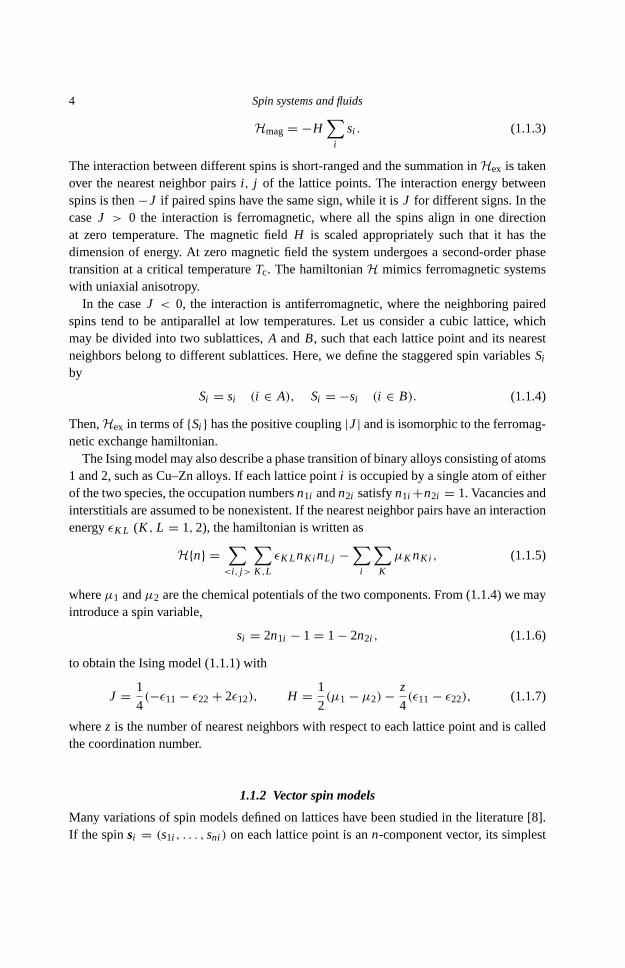
Hmag= −H∑i

si . (1.1.3)

The interaction between different spins is short-ranged and the summation inHex is takenover the nearest neighbor pairsi, j of the lattice points. The interaction energy betweenspins is then−J if paired spins have the same sign, while it isJ for different signs. In thecaseJ > 0 the interaction is ferromagnetic, where all the spins align in one directionat zero temperature. The magnetic fieldH is scaled appropriately such that it has thedimension of energy. At zero magnetic field the system undergoes a second-order phasetransition at a critical temperatureTc. The hamiltonianH mimics ferromagnetic systemswith uniaxial anisotropy.In the caseJ < 0, the interaction is antiferromagnetic, where the neighboring paired

spins tend to be antiparallel at low temperatures. Let us consider a cubic lattice, whichmay be divided into two sublattices,A andB, such that each lattice point and its nearestneighbors belong to different sublattices. Here, we define the staggered spin variablesSiby

Si = si (i ∈ A), Si = −si (i ∈ B). (1.1.4)

Then,Hex in terms of{Si } has the positive coupling|J| and is isomorphic to the ferromag-netic exchange hamiltonian.The Isingmodel may also describe a phase transition of binary alloys consisting of atoms

1 and 2, such as Cu–Zn alloys. If each lattice pointi is occupied by a single atom of eitherof the two species, the occupation numbersn1i andn2i satisfyn1i +n2i = 1. Vacancies andinterstitials are assumed to be nonexistent. If the nearest neighbor pairs have an interactionenergyεK L (K , L = 1,2), the hamiltonian is written as

H{n} =∑<i, j>

∑K ,L

εK LnKi nL j −∑i

∑K

µKnKi , (1.1.5)

whereµ1 andµ2 are the chemical potentials of the two components. From (1.1.4) we mayintroduce a spin variable,

si = 2n1i − 1= 1− 2n2i , (1.1.6)

to obtain the Ising model (1.1.1) with

J = 1

4(−ε11− ε22+ 2ε12), H = 1

2(µ1 − µ2) − z

4(ε11− ε22), (1.1.7)

wherez is the number of nearest neighbors with respect to each lattice point and is calledthe coordination number.

1.1.2 Vector spin models

Many variations of spin models defined on lattices have been studied in the literature [8].If the spinsi = (s1i , . . . , sni ) on each lattice point is ann-component vector, its simplest

1.1 Spin models 5

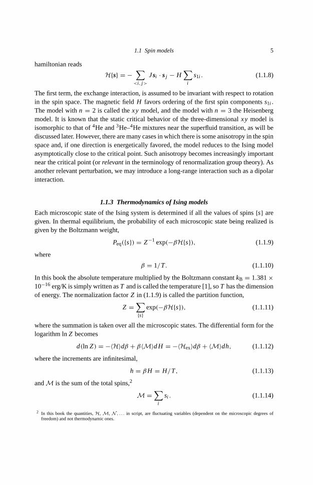
hamiltonian reads

H{s} = −∑<i, j>

Jsi · sj − H∑i

s1i . (1.1.8)

The first term, the exchange interaction, is assumed to be invariant with respect to rotationin the spin space. The magnetic fieldH favors ordering of the first spin componentss1i .The model withn = 2 is called thexymodel, and the model withn = 3 the Heisenbergmodel. It is known that the static critical behavior of the three-dimensionalxy model isisomorphic to that of4He and3He–4He mixtures near the superfluid transition, as will bediscussed later. However, there aremany cases in which there is some anisotropy in the spinspace and, if one direction is energetically favored, the model reduces to the Ising modelasymptotically close to the critical point. Such anisotropy becomes increasingly importantnear the critical point (orrelevantin the terminology of renormalization group theory). Asanother relevant perturbation, we may introduce a long-range interaction such as a dipolarinteraction.

1.1.3 Thermodynamics of Ising models

Each microscopic state of the Ising system is determined if all the values of spins{s} aregiven. In thermal equilibrium, the probability of each microscopic state being realized isgiven by the Boltzmann weight,

Peq({s}) = Z−1 exp(−βH{s}), (1.1.9)

where

β = 1/T. (1.1.10)

In this book the absolute temperature multiplied by the Boltzmann constantkB = 1.381×10−16 erg/K is simply written asT and is called the temperature [1], soT has the dimensionof energy. The normalization factorZ in (1.1.9) is called the partition function,

Z =∑{s}

exp(−βH{s}), (1.1.11)

where the summation is taken over all the microscopic states. The differential form for thelogarithm lnZ becomes

d(ln Z) = −〈H〉dβ + β〈M〉dH = −〈Hex〉dβ + 〈M〉dh, (1.1.12)

where the increments are infinitesimal,

h = βH = H/T, (1.1.13)

andM is the sum of the total spins,2

M =∑i

si . (1.1.14)

2 In this book the quantities,H, M, N , . . . in script, are fluctuating variables (dependent on the microscopic degrees offreedom) and not thermodynamic ones.

6 Spin systems and fluids

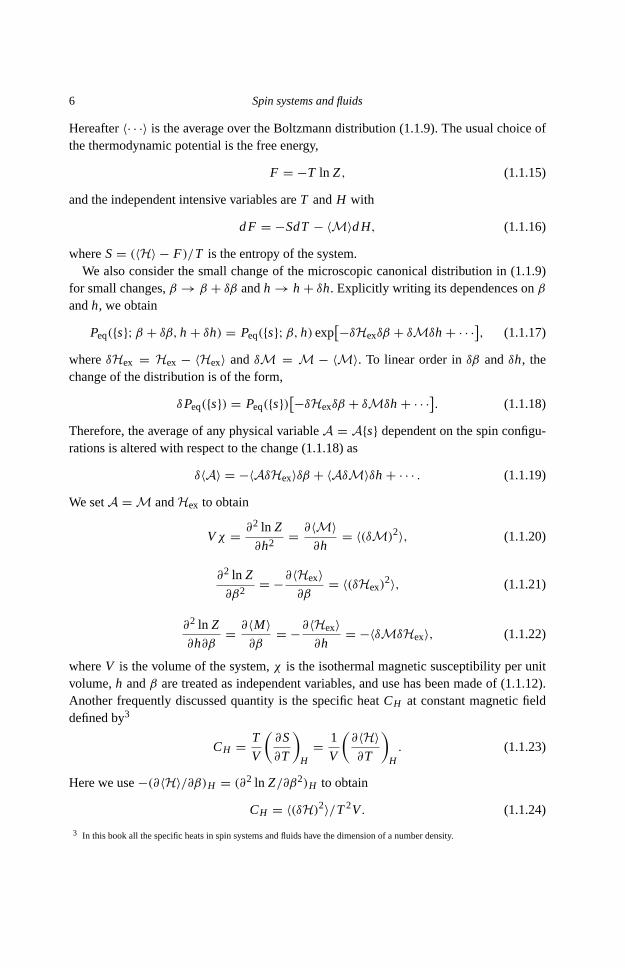
Hereafter〈· · ·〉 is the average over the Boltzmann distribution (1.1.9). The usual choice ofthe thermodynamic potential is the free energy,

F = −T ln Z, (1.1.15)

and the independent intensive variables areT andH with

dF = −SdT− 〈M〉dH, (1.1.16)

whereS= (〈H〉 − F)/T is the entropy of the system.We also consider the small change of the microscopic canonical distribution in (1.1.9)

for small changes,β → β + δβ andh → h + δh. Explicitly writing its dependences onβandh, we obtain

Peq({s};β + δβ, h + δh) = Peq({s};β, h)exp[−δHexδβ + δMδh + · · ·], (1.1.17)

whereδHex = Hex − 〈Hex〉 andδM = M − 〈M〉. To linear order inδβ andδh, thechange of the distribution is of the form,

δPeq({s}) = Peq({s})[−δHexδβ + δMδh + · · ·]. (1.1.18)

Therefore, the average of any physical variableA = A{s} dependent on the spin configu-rations is altered with respect to the change (1.1.18) as

δ〈A〉 = −〈AδHex〉δβ + 〈AδM〉δh + · · · . (1.1.19)

We setA = M andHex to obtain

Vχ = ∂2 ln Z

∂h2= ∂〈M〉

∂h= 〈(δM)2〉, (1.1.20)

∂2 ln Z

∂β2= −∂〈Hex〉

∂β= 〈(δHex)

2〉, (1.1.21)

∂2 ln Z

∂h∂β= ∂〈M〉

∂β= −∂〈Hex〉

∂h= −〈δMδHex〉, (1.1.22)

whereV is the volume of the system,χ is the isothermal magnetic susceptibility per unitvolume,h andβ are treated as independent variables, and use has been made of (1.1.12).Another frequently discussed quantity is the specific heatCH at constant magnetic fielddefined by3

CH = T

V

(∂S

∂T

)H

= 1

V

(∂〈H〉∂T

)H. (1.1.23)

Here we use−(∂〈H〉/∂β)H = (∂2 ln Z/∂β2)H to obtain

CH = 〈(δH)2〉/T2V. (1.1.24)

3 In this book all the specific heats in spin systems and fluids have the dimension of a number density.

1.1 Spin models 7

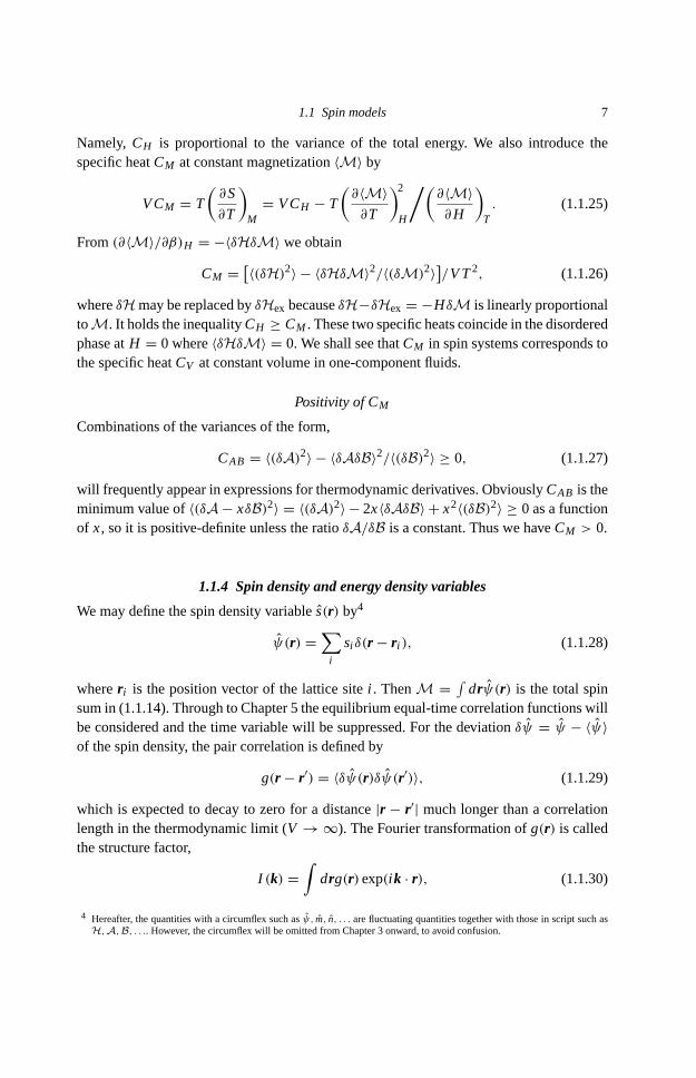
Namely,CH is proportional to the variance of the total energy. We also introduce thespecific heatCM at constant magnetization〈M〉 by

VCM = T

(∂S

∂T

)M

= VCH − T

(∂〈M〉∂T

)2H

/(∂〈M〉∂H

)T. (1.1.25)

From(∂〈M〉/∂β)H = −〈δHδM〉 we obtainCM = [〈(δH)2〉 − 〈δHδM〉2/〈(δM)2〉]/VT2, (1.1.26)

whereδHmay be replaced byδHex becauseδH−δHex = −HδM is linearly proportionaltoM. It holds the inequalityCH ≥ CM . These two specific heats coincide in the disorderedphase atH = 0 where〈δHδM〉 = 0. We shall see thatCM in spin systems corresponds tothe specific heatCV at constant volume in one-component fluids.

Positivity of CM

Combinations of the variances of the form,

CAB = 〈(δA)2〉 − 〈δAδB〉2/〈(δB)2〉 ≥ 0, (1.1.27)

will frequently appear in expressions for thermodynamic derivatives. ObviouslyCAB is theminimum value of〈(δA − xδB)2〉 = 〈(δA)2〉 − 2x〈δAδB〉 + x2〈(δB)2〉 ≥ 0 as a functionof x, so it is positive-definite unless the ratioδA/δB is a constant. Thus we haveCM > 0.

1.1.4 Spin density and energy density variables

We may define the spin density variables(r) by4

ψ(r) =∑i

si δ(r − ri ), (1.1.28)

wherer i is the position vector of the lattice sitei . ThenM = ∫drψ(r) is the total spin

sum in (1.1.14). Through to Chapter 5 the equilibrium equal-time correlation functions willbe considered and the time variable will be suppressed. For the deviationδψ = ψ − 〈ψ〉of the spin density, the pair correlation is defined by

g(r − r′) = 〈δψ(r)δψ(r′)〉, (1.1.29)

which is expected to decay to zero for a distance|r − r′| much longer than a correlationlength in the thermodynamic limit (V → ∞). The Fourier transformation ofg(r) is calledthe structure factor,

I (k) =∫

drg(r)exp(i k · r), (1.1.30)

4 Hereafter, the quantities with a circumflex such asψ, m, n, . . . are fluctuating quantities together with those in script such asH,A,B, . . .. However, the circumflex will be omitted from Chapter 3 onward, to avoid confusion.

8 Spin systems and fluids

which is expected to be isotropic (or independent of the direction ofk) at long wavelengths(ka � 1,a being the lattice constant). The susceptibility (1.1.20) is expressed as

χ =∫

drg(r) = limk→0

I (k). (1.1.31)

However, in the thermodynamic limit,χ is long-range and the space integral in (1.1.31) isdivergent at the critical point. We may also introduce the exchange energy densitye(r) by

e(r) = −∑<i, j>

Jsi sj δ(r − ri ). (1.1.32)

Then,∫dre(r) = Hex, and the (total) energy density is

eT(r) = e(r) − H ψ(r), (1.1.33)

including the magnetic field energy. From (1.1.24)CH is expressed in terms of the devia-tion δeT = eT − 〈eT〉 as

CH = T−2∫

dr〈δeT(r + r0)δeT(r0)〉, (1.1.34)

which is independent ofr0 in the thermodynamic limit.Hereafter, we will use the following abbreviated notation (also for fluid systems),

〈a : b〉 =∫

dr〈δa(r)δb(r′)〉, (1.1.35)

defined for arbitrary density variablesa(r) andb(r), which are determined by the micro-scopic degrees of freedom at the space positionr. The space correlation〈δa(r)δb(r′)〉 istaken as its thermodynamic limit, and it is assumed to decay sufficiently rapidly for large|r − r′| ensuring the existence of the long-wavelength limit (1.1.35). Furthermore, for anythermodynamic functiona = a(ψ,e), we may introduce a fluctuating variable by

a(r) = a +(∂a

∂ψ

)eδψ(r) +

(∂a

∂e

)ψ

δe(r), (1.1.36)

wherea is treated asa function of the thermodynamic averagesψ = 〈ψ〉 ande= 〈e〉. From(1.1.19) its incremental change for small variations,δβ = −δT/T2 andδh, is written as

δ〈a〉 = 〈a : e〉δTT2

+ 〈a : ψ〉δh + · · · . (1.1.37)

From the definition, the above quantity is equal toδa = (∂a/∂T)hδT+(∂a/∂h)Tδh. Thus,

T2(∂a

∂T

)h

= 〈a : e〉,(∂a

∂h

)T

= 〈a : ψ〉. (1.1.38)

1.1 Spin models 9

The variances amongψ andeare expressed as

χ =(∂ψ

∂h

)T

= 〈ψ : ψ〉, T2(∂e

∂T

)h

= 〈e : e〉,

T2(∂ψ

∂T

)h

=(∂e

∂h

)T

= 〈ψ : e〉. (1.1.39)

The specific heats are rewritten as

CH = 1

T2〈eT : eT〉, CM = 1

T2

[〈e : e〉 − 〈e : ψ〉2/〈ψ : ψ〉]. (1.1.40)

1.1.5 Hydrodynamic fluctuations of temperature and magnetic field

In the book by Landau and Lifshitz (Ref. [1], Chap. 12), long-wavelength (or hydrody-namic) fluctuations of the temperature and pressure are introduced for one-componentfluids. For spin systems we may also consider fluctuations of the temperature and magneticfield around an equilibrium reference state. As special cases of (1.1.36) we define

δT(r) =(∂T

∂ψ

)eδψ(r) +

(∂T

∂e

)ψ

δe(r), (1.1.41)

δh(r) =(∂h

∂ψ

)eδψ(r) +

(∂h

∂e

)ψ

δe(r). (1.1.42)

We may regardδT and δ H = Tδh + hδT as local fluctuations superimposed on thehomogeneous temperatureT and magnetic fieldH = Th, respectively. Therefore, (1.1.38)yields

〈h : ψ〉 = 1

T2〈T : e〉 = 1, 〈h : e〉 = 〈T : ψ〉 = 0. (1.1.43)

More generally, the density variablea in the form of (1.1.36) satisfies

〈a : T〉 = T2(∂a

∂e

)ψ

, 〈a : h〉 =(∂a

∂ψ

)e. (1.1.44)

In particular, the temperature variance reads5

〈T : T〉 = T2/CM . (1.1.45)

The variances amongδh andδT/T constitute the inverse matrix of those amongδψ andδe/T . To write them down, it is convenient to define the determinant,

D = 1

T2

[〈ψ : ψ〉〈e : e〉 − 〈ψ : e〉2] = χCM . (1.1.46)

5 In the counterpart of this relation,CM will be replaced byCV in (1.2.64) for one-component fluids and byCVX in (1.3.44)for binary fluid mixtures.

10 Spin systems and fluids

The elements of the inverse matrix are written as6

Vττ ≡ 1

T2〈T : T〉 = 1

CM, Vhh ≡ 〈h : h〉 = 〈e : e〉/T2D,

Vhτ ≡ 1

T〈T : h〉 = −〈ψ : e〉/TD. (1.1.47)

In the disordered phase withT > Tc andH = 0, we have no cross correlation〈ψ : e〉 =0, so thatVττ = 1/CH , Vhh = 1/χ , andVhτ = 0. For other values ofT andH , there isa nonvanishing cross correlation (Vhτ �= 0). The following dimensionless ratio representsthe degree of mixing of the two variables,

Rv = 〈ψ : e〉2/[〈ψ : ψ〉〈e : e〉]

= T2(∂ψ

∂T

)2

h

/(∂ψ

∂h

)T

(∂e

∂T

)h, (1.1.48)

where 0≤ Rv ≤ 1 and use has been made of (1.1.39) in the second line. From (1.1.40) wehave

CM = CH (1− Rv), (1.1.49)

for h = 0 (or for sufficiently smallh, as in the critical region). In Chapter 4 we shall seethat Rv ∼= 1/2 asT → Tc on the coexistence curve (T < Tc andh = 0) in 3D Isingsystems.In the long-wavelength limit, the probability distribution of the gross variables,ψ(r)

andm(r), tends to be gaussian with the form exp(−βHhyd), where the fluctuations withwavelengthsshorter than the correlation length have been coarse-grained. From (1.1.39),(1.1.43), and (1.1.46) thehydrodynamic hamiltonianHhyd in terms of δψ and δT isexpressed as

Hhyd = T∫

dr{1

2χ[δψ(r)]2 + 1

2T2CM [δT(r)]2

}. (1.1.50)

Another expression forHhyd can also be constructed in terms ofδeandδh.

1.2 One-component fluids

1.2.1 Canonical ensemble

Nearly-spherical molecules, such as rare-gas atoms, may be assumed to interact via apairwise potentialv(r ) dependent only on the distancer between the two particles [4]–[6].It consists of a short-range hard-core-like repulsion (r � σ ) and a long-range attraction(r � σ ). These two behaviors may be incorporated in the Lenard-Jones potential,

v(r ) = 4ε

[(σ

r

)12

−(σ

r

)6]. (1.2.1)

6 These relations will be used in (2.2.29)–(2.2.36) for one-component fluids and in (2.3.33)–(2.3.38) for binary fluid mixturesafter setting up mapping relations between spin and fluid systems.

1.2 One-component fluids 11

This pairwise potential is characterized by the core radiusσ and the minimum−ε attainedat r = 21/6σ . In classical mechanics, the hamiltonian forN identical particles with massm0 is written as

H = 1

2m0

∑i

|pi |2 +∑<i, j>

v(ri j ), (1.2.2)

wherepi is the momentum vector of thei th particle,ri j is the distance between the particlepair i, j, and<i, j> denotes summation over particle pairs. The particles are confined ina container with a fixed volumeV and the wall potential is not written explicitly in (1.2.2).In the canonical ensembleT , V , and N are fixed, and the statistical distribution is

proportional to the Boltzmann weight as [1]–[3]

Pca(�) = 1

ZNexp[−βH], (1.2.3)

in the 2dN-dimensional phase space� = (p1 · · ·pN, r1 · · · rN) (sometimes called the�-space). The spatial dimensionality is written asd and may be general. The partitionfunction ZN of N particles for the canonical ensemble is then given by the multipleintegrations,

ZN = 1

N!(2π h)dN

∫dp1 · · ·

∫dpN

∫dr1 · · ·

∫drN exp(−βH)

= 1

N!λdNth

∫dr1 · · ·

∫drN exp(−βU), (1.2.4)

whereh = 1.05457×10−27 erg s is the Planck constant. In the second line the momentumintegrations over the maxwellian distribution have been performed, where

λth = h(2π/m0T)1/2 (1.2.5)

is called the thermal de Broglie wavelength, and

U =∑<i, j>

v(ri j ) (1.2.6)

is the potential part of the hamiltonian.The Helmholtz free energy is given byF = −T ln ZN . The factor 1/N!(2π h)dN

in (1.2.4) naturally arises in the classical limit(h → 0) of the quantum mechanicalpartition function [2]. Physically, the factor 1/N! represents the indistinguishability be-tween particles, which assures the extensive property of the entropy. That is, a set ofclassical microscopic states obtainable only by the particle exchange,i → j and j → i ,corresponds to a single quantum microscopic state.7 The factor 1/(2π h)dN is ascribed tothe uncertainty principle (�p�x ∼ 2π h).

7 The concept of indistinguishability is intrinsically of quantum mechanical origin as well as the uncertainty principle. It is notnecessarily required in the realm of classical statistical mechanics. Observable quantities such as the pressure are not affectedby the factor1/N!.

12 Spin systems and fluids

1.2.2 Grand canonical ensemble

A fluid region can be in contact with a mass reservoir characterized by a chemical potentialµ as well as with a heat reservoir at a temperatureT . As an example of such a system,we may choose an arbitrary macroscopic subsystem with a volume much smaller than thevolume of the total system. In this case we should consider the grand canonical distribution,in which T , µ, andV are fixed and the energy and the particle number are fluctuatingquantities. To make this explicit, the particle number will be written asN and, to avoid toomany symbols, the average〈N 〉 will be denoted byN which is now a function ofT andµ. The statistical probability of each microscopic state withN particles being realized isgiven by [1]–[3]

Pgra(�) = 1

�exp[−βH + βµN ]. (1.2.7)

The equilibrium average is written as〈· · ·〉 = ∫d�(· · ·)Pgra(�), where∫

d� =∑N

1

N !(2π h)dN

∫dp1 · · ·

∫dpN

∫dr1 · · ·

∫drN (1.2.8)

represents the integration of the configurations in the�-space. The normalization factor orthe grand partition function� is expressed as

� =∑N

ZN exp(Nβµ). (1.2.9)

In this summation the contribution aroundN ∼= N = 〈N 〉 is dominant for largeN, andthe logarithm� ≡ ln� satisfies

� = ln ZN + Nβµ = pV/T, (1.2.10)

in the thermodynamic limitN → ∞. Use has been made of the fact thatG = Nµ is theGibbs free energy.We may choose� as a thermodynamic potential dependent onβ and

ν = βµ = µ/T. (1.2.11)

Then, analogous to (1.1.12) for Ising systems, the differential form for� is written as[9, 10]

d� = −〈H〉dβ + 〈N 〉dν, (1.2.12)

where

〈H〉 = 3

2〈N 〉T + 〈U〉 (1.2.13)

is the energy consisting of the average kinetic energy and the average potential energy.Notice that (1.2.12) may be transformed into the well-known Gibbs–Duhem relation,

dµ = 1

ndp− sdT, (1.2.14)

1.2 One-component fluids 13

wheren = 〈N 〉/V is the average number density ands = (〈H〉 − F)/NT is the entropyper particle.We then find the counterparts of (1.1.20)–(1.1.22) among the thermodynamic derivatives

and the fluctuation variances ofδN = N − 〈N 〉 andδH = H − 〈H〉 as∂2�

∂ν2= ∂〈N 〉

∂ν= 〈(δN )2〉, (1.2.15)

∂2�

∂β2= −∂〈H〉

∂β= 〈(δH)2〉, (1.2.16)

− ∂2�

∂ν∂β= −∂〈N 〉

∂β= ∂〈H〉

∂ν= 〈δN δH〉, (1.2.17)

where all the quantities are regarded as functions ofβ, andν = βµ and the volumeV isfixed.The isothermal compressibility is expressed as

KT = 1

n

(∂n

∂p

)VT

= β

n2

(∂

∂ν

〈N 〉V

)β

, (1.2.18)

wheren = 〈N 〉/V is the average number density and use has been made of (1.2.14). Thefluctuation variance ofδN = N − 〈N 〉 is expressed in terms ofKT as

〈(δN )2〉 = Vn2T KT (grand canonical). (1.2.19)

As forCM in (1.1.26), the constant-volume specific heatCV = (∂〈H〉/∂T)VN/V per unitvolume can be calculated in terms of the fluctuation variances as

CV = [〈(δH)2〉 − 〈δHδN 〉2/〈(δN )2〉]/VT2 (grand canonical), (1.2.20)

where use has been made of

(∂〈H〉/∂T)N = (∂〈H〉/∂T)ν + (∂〈H〉/∂N)T(∂N/∂T)ν.

Field variables and density variables

Following Griffiths and Wheeler [10] and Fisher [11], we refer toT (or β) and h inspin systems andT (or β), p, ν, . . . in fluids asfields, which have identical values intwo coexistingphases. We refer to the spin and energy densities in spin systems andthe densities of number, energy, entropy,. . . in fluids asdensities. In spin systems, theaverage spin is discontinuous between the two coexisting phases, but the average energy iscontinuous. In fluids, the density variables usually have different average values in the twocoexisting phases, but can be continuous in accidental cases such as the azeotropic case(see Section 2.3). In this book the density variables (even the entropy and concentration)have microscopic expressions in terms of the spins or the particle positions and momenta.Their equilibrium averages become the usual thermodynamic variables, and their equi-librium fluctuation variances can be related to somethermodynamic derivatives in thelong-wavelength limit.

14 Spin systems and fluids

Shift of the origin of the one-particle energy

It would also be appropriate to remark on the arbitrariness of the origin of the energysupported by each particle. That is, let us shift the hamiltonian as

H → H + ε0N (1.2.21)

and the chemical potential fromµ to µ + ε0. Then,ε0 vanishes in the grand canonicaldistribution and hencemeasurable quantities such as the pressurep should remain invariantor independent ofε0 as long as they do not involve the origin of the one-particle energy.We can see that the terms involvingε0 cancel in the variance combination (1.2.20), soCV

is clearly independent ofε0.

Lattice gas model

In the lattice gas model [12], particles are distributed on fixed lattice points in evaluatingthe potential energy contribution to�. The lattice constanta is taken to be the hard-coresize of the pair potential, so each lattice point is supposed to be either vacant (ni = 0) oroccupied (ni = 1) by a single particle. Then� is approximated as

� =∑{n}

exp(−βH{n}), (1.2.22)

with

H{n} = −∑<i, j>

εni n j − (µ + dT ln λth)∑i

ni , (1.2.23)

where the summation in the first term is taken over the nearest neighbor pairs andε

represents the magnitude of the attractive part of the pair potential. Obviously, if we setsi = 2ni − 1, the above hamiltonian becomes isomorphic to the spin hamiltonian (1.1.1)underJ = ε/4 and

H = 1

2µ + d

2T ln λth − 1

4zε = 1

2µ − d

4T ln T + const., (1.2.24)

z being the coordination number. The pressurep in the lattice gas model is related to thefree energyFIsing of the corresponding Ising spin system by

p = −V−1FIsing+ a−d(H + 1

8zε

). (1.2.25)

1.2.3 Thermodynamic derivatives and fluctuation variances

Analogously to the spin case (1.1.18), the grand canonical distribution functionPgra(�) in(1.2.7) is changed against small changes,β → β + δβ andν → ν + δν, as [9]

δPgra = [−δHδβ + δN δν]Pgra, (1.2.26)

1.2 One-component fluids 15

where only the linear deviations are written. Because the choice ofβ andν as independentfield variables is not usual, we may switch to the usual choice,T andp. HereδT = −T2δβ

and

δp = nT(δν − Hδβ), (1.2.27)

where

H = µ + Ts (1.2.28)

is the enthalpy per particle and should not be confused with the magnetic field in the spinsystem, ands is the entropy per particle. Then (1.2.26) is rewritten as

δPgra =[nδS δT

T+ δN δp

nT

]Pgra, (1.2.29)

where

δS = 1

nT[δH − HδN ] (1.2.30)

is the space integral of the entropy density variable to be introduced in (1.2.46) below.Thus, the thermodynamic average of any fluctuating quantityA changes as

δ〈A〉 = −〈AδH〉δβ + 〈AδN 〉δν + · · · ,

= 〈AδS〉nδTT

+ 〈AδN 〉 δpnT

+ · · · . (1.2.31)

Note thatδS is invariant with respect to the energy shift in (1.2.21) because the enthalpyH is also shifted byε0.The familiar constant-pressure specific heatCp = nT(∂s/∂T)p per unit volume is

obtained fromVCp = nT limδT→0 〈δS〉/δT with δp = 0. From the second line of (1.2.31)Cp becomes

Cp = n2〈(δS)2〉/V = 〈(δH − HδN )2〉/VT2 (grand canonical). (1.2.32)

In terms ofδS, the constant-volume specific heatCV is also expressed as

CV = n2[〈(δS)2〉 − 〈δSδN 〉2/〈(δN )2〉]/V (grand canonical), (1.2.33)

which is equivalent to (1.2.20). It leads to the inequalityCp ≥ CV . Use of thethermodynamic identityCp/CV = KT/Ks yields the adiabatic compressibilityKs =(∂n/∂p)s/n in the form

Ks = [〈(δN )2〉 − 〈δSδN 〉2/〈(δS)2〉]/Vn2T (grand canonical). (1.2.34)

The sound velocityc is given byc = (ρKs)−1/2, ρ = m0n being the mass density.

16 Spin systems and fluids

1.2.4 Gaussian distribution in the long-wavelength limit

We next consider the equilibrium statistical distribution function for the macroscopicgross variables,H andN , for one-component fluids, which we write asP(H,N ). TheentropyS(E, N) as a function ofE andN is the logarithm of the number of microscopicconfigurations atH = E andN = N. It may be written as

exp[S(E, N)] =∫

d�δ(H − E)δ(N − N), (1.2.35)

whered� is the configuration integral (1.2.8). This grouping of the microscopic statesgives

P(H,N ) = 1

�exp[S(H,N ) − βH + νN ], (1.2.36)

with the grand canonical partition function,

� =∫

dH∫

dN exp[S(H,N ) − βH + νN ]. (1.2.37)

Each thermodynamic state is characterized byβ andν or by E = 〈H〉 andN = 〈N 〉. Wethen expandS(H,N ) with respect to the deviationsδH = H − E andδN = N − N as

S(H,N ) = S(E, N) + βδH − νδN + (�S)2 + · · · , (1.2.38)

where(δS)2 is the bilinear part,

(�S)2 = 1

2

(∂2S

∂E2

)(δH)2 +

(∂2S

∂E∂N

)δHδN + 1

2

(∂2S

∂N2

)(δN )2. (1.2.39)

In the probability distribution (1.2.36) the linear terms cancel if (1.2.38) is substituted, sothe distribution becomes the following well-known gaussian form [1, 3, 7]:

P(H,N ) ∝ exp[(�S)2]. (1.2.40)

From this distribution we can re-derive (1.2.15)–(1.2.17) by using the relations,

αee ≡ V∂2S

∂E2= ∂β

∂e, αnn ≡ V

∂2S

∂N2= −∂ν

∂n,

αen ≡ V∂2S

∂N∂E= ∂β

∂n= −∂ν

∂e, (1.2.41)

whereβ andν are regarded as functions ofn = N/V ande= E/V . The three coefficientsin (1.2.41) divided by−V constitute the inverse of the matrix whose elements are thevariances amongH andN .

Weakly inhomogeneous cases

The above result may be generalized for weakly inhomogeneous cases as follows. Let usconsider a small fluid element whose linear dimension is much longer than the correlationlength. Because the thermodynamics in the element is described by the grand canonical

1.2 One-component fluids 17

ensemble, the long-wavelength, number and energy density fluctuations,δn(r) andδe(r),obey a gaussian distribution of the form (1.2.40) with

(�S)2 =∫

dr[1

2αee(δe(r))2 + αenδe(r)δn(r) + 1

2αnn(δn(r))2

]. (1.2.42)

Thermodynamic stability

It has been taken for granted that the probability distribution (1.2.36) is maximum for theequilibrium values, which results in the positive-definiteness of the matrix composed of thecoefficients in (1.2.41). In thermodynamics [2, 13] this positive-definiteness (implying thepositivity ofCV , KT , etc.) follows from the thermodynamic stability of equilibrium states.In this book, because we start with statistical–mechanical principles, their positivity is anobvious consequence evident from their variance expressions.

1.2.5 Fluctuating space-dependent variables

The number density variablen(r) and the energy density variablee(r) have microscopicexpressions,

n(r) =∑i

δ(r − ri ), (1.2.43)

e(r) =∑i

1

2m0|pi |2δ(r − ri ) + 1

2

∑i �= j

v(ri j )δ(r − ri ), (1.2.44)

in terms of the particle positions and momenta. As in (1.1.36) we may introduce a fluctu-ating variable by

a(r) = a +(∂a

∂n

)eδn(r) +

(∂a

∂e

)nδe(r), (1.2.45)

for any thermodynamic variablea given as a function of the averagesn = 〈n〉 ande= 〈e〉.The nonlinear termssuch as(∂2a/∂n2)(δn)2 are not included in the definition. Fromds=(de− Hdn)/nT the space-dependent entropy variable is introduced by

s(r) = s+ 1

nT

[δe(r) − Hδn(r)

], (1.2.46)

whereH = µ+Ts= (e+ p)/n is the enthalpy per particle. The space integral ofδs(r) =s(r) − s is equal toδS in (1.2.30). In terms of these density variables, the incrementalchange of the grand canonical distribution in (1.2.26) and (1.2.29) is expressed as

δPgra = Pgra

∫dr[−δe(r)δβ + δn(r)δν]

= Pgra

∫dr

[nδs(r)

δT

T+ δn(r)

δp

nT

], (1.2.47)

18 Spin systems and fluids

whereδp is the pressure deviation defined in (1.2.27). With these two expressions we mayexpress any thermodynamic derivatives in terms of fluctuation variances ofn, e, ands inthe long-wavelength limit. Using the notation〈 : 〉, as in (1.1.35), we have

KT = (n2T)−1〈n : n〉, Cp = n2〈s : s〉, αp = −T−1〈s : n〉, (1.2.48)

where αp = −(∂n/∂T)p/n is the thermal expansion coefficient. From (1.2.20) and(1.2.33) the constant-volume specific heat is expressed as

CV = T−2[〈e : e〉 − 〈e : n〉2/〈n : n〉]= n2

[〈s : s〉 − 〈s : n〉2/〈n : n〉]. (1.2.49)

The first line was obtained by Schofield [see Ref. 18]. From (1.2.34) the adiabatic com-pressibility is expressed as

Ks = (ρc2)−1 = [〈n : n〉 − 〈n : s〉2/〈s : s〉]/n2T. (1.2.50)

These expressions are in terms of the long-wavelength limit of the correlation functions.Hence, to their merit, they tend to unique thermodynamic limits, whether the ensemble iscanonical or grand canonical, asN,V → ∞ with a fixed densityn = N/V .More generally, for any density variablea in the form of (1.2.45), we obtain

〈a : e〉 = T2(∂a

∂T

)ν

, 〈a : n〉 = nT

(∂a

∂p

)T, 〈a : s〉 = 1

nT

(∂a

∂T

)p. (1.2.51)

It then follows that(∂p

∂T

)a

= −(∂a

∂T

)p

/(∂a

∂p

)T

= −n2〈a : s〉/〈a : n〉. (1.2.52)

Finally, we give some thermodynamic identities,

ρc2CV = T

(∂p

∂T

)s

(∂p

∂T

)n

= T

(∂p

∂T

)2

s(1− CV/Cp), (1.2.53)

CV/Cp = Ks/KT = 1−(∂p

∂T

)n

/(∂p

∂T

)s. (1.2.54)

These are usually proved with the Maxwell relations but can also be derived from thevariance relations (1.2.48)–(1.2.54).

1.2.6 Density correlation

In the literature [4]–[6] special attention has been paid to the radial distribution functiong(r ) defined by

n2g(|r − r′|) =∑i �= j

〈δ(r − ri )δ(r′ − r j )〉

= 〈n(r)n(r′)〉 − nδ(r − r′), (1.2.55)

1.2 One-component fluids 19

where the self-part (i = j ) has been subtracted andg(r ) → 1 at long distance in thethermodynamic limit.8 The structure factor is expressed as

I (k) =∫

drei k·r〈δn(r)δn(0)〉 = n + n2∫

drei k·r [g(r ) − 1]. (1.2.56)

An example ofI (k) can be found in Fig. 2.3. The isothermal compressibility (1.2.18) isexpressed as

KT = (n2T)−1 limk→0

I (k) = (nT)−1 + T−1∫

dr[g(r ) − 1]. (1.2.57)

The physical meaning ofg(r ) is as follows.We place a particle at the origin of the referenceframe and consider a volume elementdr at a positionr; then,ng(r )dr is the averageparticle number in the volume element. In liquid theories another important quantity isthe direct correlation functionC(r ) defined by

g(r ) = C(r ) +∫

dr′C(|r − r′|)ng(|r′|). (1.2.58)

Its Fourier transformationCk satisfies

I (k) = n/(1− nCk). (1.2.59)

Let us assume naively thatC(r ) decays more rapidly than the pair correlation functiong(r )at long distances andCk can be expanded asCk = C0−C1k2+· · · at smallk with C1 > 0[14]. Then, (1.2.59) yields a well-known expression called the Ornstein–Zernike form,

I (k) ∼= n/(1− nC0 + nC1k2), (1.2.60)

at smallk. Notice thatC0 = limk→0Ck approaches ton−1 as the critical point (or thespinodal linemore generally) is approached. The direct correlation functions for binarymixtures will be discussed at the end of Section 1.3.

1.2.7 Hydrodynamic temperature and pressure fluctuations

As in the book by Landau and Lifshitz [1], we introduce the temperature fluctuationδT asa space-dependent variable by

δT(r) =(∂T

∂e

)nδe(r) +

(∂T

∂n

)eδn(r)

= nT

CV

[δs(r) + 1

n2

(∂p

∂T

)nδn(r)

], (1.2.61)

where the energy densitye(r), the number densityn(r), and the entropy densitys(r) aredefined by (1.2.45)–(1.2.47), and use has been made of(∂s/∂n−1)T = (∂p/∂T)n. We as-sume that these density variables consist only of the Fourier components with wavelengths

8 In a finite system, the space integral of (1.2.55) in the volumeV would becomeN(N − 1)/V , in apparent contradiction to(1.2.57).

20 Spin systems and fluids

much longer than any correlation lengths (q � ξ−1, near the critical point,ξ being thecorrelation length). Thena in the form of (1.2.45) satisfies

〈a : T〉 = T

n

(∂a

∂s

)n

= T2

CV

(∂a

∂T

)n. (1.2.62)

This relation gives [1]

〈n : T〉 = 0, 〈s : T〉 = T/n, (1.2.63)

〈T : T〉 = T2/CV , (1.2.64)

The long-wavelength fluctuations obey a gaussian distribution∝ exp[−βHhyd]. Thehydrodynamic hamiltonian is written as

Hhyd =∫

dr{CV

2T[δT(r)]2 + 1

2n2KT[δn(r)]2

}, (1.2.65)

which is analogous to (1.1.50) for Ising systems.We may also introduce a hydrodynamic pressure variableδ p(r) by

δ p(r) =(∂p

∂e

)nδe(r) +

(∂p

∂n

)eδn(r)

= ρc2[1

nδn(r) + n

(∂T

∂p

)sδs(r)

], (1.2.66)

whereρ is the mass density and use has been made of(∂n−1/∂s)p = (∂T/∂p)s. For a(r)in the form of (1.2.45) we obtain

〈a : p〉 = Tn

(∂a

∂n

)s

= Tρc2(∂a

∂p

)s. (1.2.67)

Substitutinga = p andT yields

〈 p : p〉 = ρc2T, (1.2.68)

〈 p : T〉 = Tρc2(∂T

∂p

)s

= T2

CV

(∂p

∂T

)n. (1.2.69)

By settinga = s andn we also notice

〈s : p〉 = 0, 〈n : p〉 = nT. (1.2.70)

TheHhyd may be rewritten in another orthogonal form,

Hhyd =∫

dr{

1

2ρc2[δ p(r)]2 + n2T

2Cp[δs(r)]2

}. (1.2.71)

It goes without saying that(�S)2 in (1.2.42) coincides with−βHhyd.

1.2 One-component fluids 21

1.2.8 Projection onto gross variables in the hydrodynamic regime

The pressure fluctuation variableδ p(r) in (1.2.66) may be interpreted as theprojectionofthe microscopic stress tensor�αβ(r) (α, β = x, y, z) onto the gross variablesδe (or δs)andδn.9 In the hydrodynamic regime, for any fluctuating variablea(r) dependent on space,the projection operatorP is defined as

Pa(r) = 〈a〉 + Aenδe(r) + Aneδn(r). (1.2.72)

The two coefficientsAen andAne are determined such that the right-hand side andδa havethe same correlations withδe andδn. ThenP2 = P. If a is of the form (1.2.45), we havePa = a. We neglect nonlocality in (1.2.72) assuming thatδeandδn consist of the Fouriercomponents with an upper cut-off wave number� much smaller than the inverse thermalcorrelation length. The calculation of the coefficients is simplified if the above relation isrewritten in terms ofδ p andδs as

Pδa(r) = Apsδ p(r) + Aspδs(r). (1.2.73)

Using〈s : p〉 = 0, we find

Aps = 〈a : p〉/〈 p : p〉, Asp = 〈a : s〉/〈s : s〉. (1.2.74)

From (1A.11) and (1A.12) in Appendix 1A, we may derive the following variancerelations,

〈n : �αβ〉 = nTδαβ, 〈e : �αβ〉 = (e+ p)Tδαβ. (1.2.75)

Then, from the definitions ofs in (1.2.46) andp in (1.2.66) we obtain

〈s : �αβ〉 = 0, 〈 p : �αβ〉 = ρc2Tδαβ. (1.2.76)

Hence, we arrive at

Pδ�αβ(r) = δαβδ p(r). (1.2.77)

This leads to the inequality

ρc2 ≤ K∞ ≡⟨∑

α

�αα :∑β

�ββ

⟩/d2T. (1.2.78)

See (1.2.84) below forK∞ [18]. In fact, at the gas–liquid critical point the sound velocityc goes to zero butK∞ remains finite. These are consistent with the inequality in (1.2.78).

1.2.9 Pressure, energy, and elastic moduli in terms ofg(r )

In Appendix 5E we will give the space-dependent microscopic expression for the stresstensor�αβ(r). Its space integral has the following microscopic expression [5, 6],∫

dr�αβ(r) =∑i

piα piβm0

−∑<i, j>

v′(ri j )1

ri jxi j αxi jβ, (1.2.79)

9 As will be discussed in Chapter 5, the projection operator method has been developed in the study of irreversible processes.

22 Spin systems and fluids

wherev′(r ) = dv(r )/dr , xiα (α = x, y, z) are the cartesian coordinates of the particleposition r i , andxi j α = xiα − xjα. The pressure is then expressed in terms of the radialdistribution functiong(r ) in (1.2.55) as

p = nT − 1

2dJ1, (1.2.80)

with

J1 =∫

drn2g(r )r v′(r ), (1.2.81)

whered in (1.2.80) is the spatial dimensionality. In addition, the internal energy density isexpressed as

e= 〈e〉 = d

2nT + 1

2

∫drn2g(r )v(r ). (1.2.82)

In an isotropic equilibrium state the variances among the stress tensor�αβ in the long-wavelength limit are written as

1

T〈�αβ : �γ δ〉 = (δαγ δβδ + δαδδβγ )G∞ + δαβδγ δ

(K∞ − 2

dG∞

). (1.2.83)

HereK∞ andG∞ are called theelastic moduliof fluids [6], [15]–[18]. Although elasticdeformations are not well defined in fluids, they were interpreted as the infinite-frequencyelastic moduli of fluids [17].10 Interestingly, they can be expressed in terms ofg(r ) as[17, 18]

K∞ = 1

d2T

⟨∑α

�αα :∑β

�ββ

⟩=

(1+ 2

d

)nT − d − 1

2d2J1 + 1

2d2J2, (1.2.84)

G∞ = 1

T〈�xy : �xy〉 = nT + 1

2d(d + 2)

[(d + 1)J1 + J2

], (1.2.85)

whereJ1 is defined by (1.2.81) and

J2 =∫

drn2g(r )r 2v′′(r ), (1.2.86)

with v′′(r ) = d2v(r )/dr2. Elimination ofJ1 andJ2 yields a general relation,

K∞ −(1+ 2

d

)G∞ = 2(p− nT). (1.2.87)

It is not trivial that K∞ andG∞ can be expressed in terms of the radial distributionfunction, although they involve correlations among four particles. We will present a generaltheory for calculating correlation functions involving the stress tensor in Appendix 1A.Schofield calculated more general wave number-dependent correlation functions among

10 In highly supercooled fluids, a shear modulus becomes well defined and measurable. It is smaller thanG∞ but larger thannT. See Fig. 11.33 and its explanation in Section 11.4.