Embed Size (px)
Citation preview
PHASE EQUILIBRIUM STUDIES OF SULFOLANE
MIXTURES CONTAINING CARBOXYLIC ACIDS
PHASE EQUILIBRIUM STUDIES OF SULFOLANE
MIXTURES CONTAINING CARBOXYLIC ACIDS
NOMPUMELELO PRETTY SITHOLE
B.Tech: Chemistry (DUT)
Submitted in fulfilment of the academic requirements for the
Masters degree in Technology
in the Department of Chemistry, Durban University of Technology,
Durban, South Africa
2012
P r e f a c e i
PREFACE
This work was done in the Department of Chemistry, Durban University of
Technology, M L Sultan Campus in Durban, KwaZulu Natal Province, South
Africa

Declaration ii
DECLARATION
I hereby certify that this research is the result of my own investigation, which has
not already been accepted in substance for any degree, and is not being
concurrently submitted for any other degree. Where use was made of the work
of others, it has been duly acknowledged in the text.
……………………………… ……………………………………..
N P Sithole Date
I hereby certify that the above statement is correct.
……………………………… ………………………………
Professor G G Redhi Date

D e d i c a t i o n iii
DEDICATION
I would like to dedicate this thesis to my late big brother Mr Mzomuhle Moses
Sithole

Acknowledgements iv
ACKNOWLEDGMENTS
I would like to record my appreciation to the following:
God Almighty for guiding me through this journey to finish this project, it
was not an easy one but His endless guidance saw me through it all.
Prof G. G. Redhi from Durban University of Technology, Chemistry
Department, my supervisor for his unlimited guidance, help, support and
patience throughout the course of the project.
My mother Mrs Zolani Sithole for her pep talk and motivation to pursue
my dreams and never to give up even if it becomes tough.
My husband Mr Thokozani Nyangayibizwa Cele for his unlimited support
and motivation throughout the course of this project.
My friends, Thabile, Cathrine, Thobeka, Nokukhanya and Myalo for their
support and help.
National Research Foundation and Durban University of Technology:
Postgraduate Department for providing me with financial support and
electronic notebook to finish this project.
The Chemistry laboratory staff from Durban University of Technology for
the help with instrumentation and motivation.
Abstract v
ABSTRACT
In this work, the thermodynamics of ternary liquid mixtures involving carboxylic
acids with sulfolane, hydrocarbons including cycloalkane, and alcohols are
presented. In South Africa, Sasol is one of the leading companies that produce
synthesis gas from low grade coal. Carboxylic acids together with many other
oxygenate and hydrocarbons are produced by Sasol using the Fischer-Tropsch
process. Carboxylic acids class is one of the important classes of compounds
with great number of industrial uses and applications. The efficient separation of
carboxylic acids from hydrocarbons and alcohols from hydrocarbons is of
economic importance in the chemical industry, and many solvents have been
tried and tested to improve such recovery. This work focussed on the use of the
polar solvent sulfolane in the effective separation by solvent extraction and not
by more common energy intensive method of distillation.
The first part of the experimental work focussed on ternary liquid-liquid equilibria
of mixtures of [sulfolane (1) + carboxylic acid (2) + heptane (3) or cyclohexane
or dodecane] at T = 303.15 K, [sulfolane (1) + alcohol (2) + heptane (3)] at T =
303.15 K. Carboxylic acid refers to acetic acid, propanoic acid, butanoic acid, 2-
methylpropanoic acid, pentanoic acid and 3-methylbutanoic acid. Alcohol refers
to methanol, ethanol, 1- propanol, 2-propanol, 1-butanol, 2-butanol, 2-methyl-1-
propanol and 2-methyl-2-propanol. Ternary liquid- liquid equilibrium data are
essential for the design and selection of solvents used from liquid- liquid
extraction process.
Abstract vi
The separation of carboxylic acids from hydrocarbons and the alcohols from
hydrocarbons is commercially lucrative consideration and is an important reason
of this study. The separation of carboxylic acids or alcohols from hydrocarbons
by extraction with sulfolane was found to be feasible as all selectivity values
obtained are greater than 1.
The modified Hlavatý, beta (β) and log equations were fitted to the
experimental binodal data measured in this work. Hlavatý gave the best overall
fit as compared to beta ( ) and log function.
The NRTL (Non-Random, Two Liquid) and UNIQUAC Universal Quasichemical)
model were used to correlate the experimental tie-lines and calculate the phase
compositions of the ternary systems. The correlation work served three
purposes:
to summarise experimental data
to test theories of liquid mixtures
prediction of related thermodynamics properties.
The final part of the study was devoted to the determination of the excess molar
volumes of mixtures of [sulfolane (1) + alcohol (2)] at T = 298.15 K, T = 303.15 K
and T = 309.15 K. Density was used to determine the excess molar volumes of
the mixtures of [sulfolane (1) + alcohols (2)]. Alcohol refers to methanol, ethanol,
1- propanol, 2-propanol, 1-butanol, 2-butanol, 2-methyl-1-propanol, 2-methyl-2-
propanol.
The work was done to investigate the effect of temperature on excess molar
volumes of binary mixtures of alcohols and sulfolane, as well as to get some
idea of interactions involved between an alcohol and sulfolane. The excess
molar volume data for each binary mixture was fitted in the Redlich–Kister
equation to correlate the composition dependence of the excess property.
Contents vii
CONTENTS
Preface (i)
Declaration (ii)
Acknowledgement (iii)
Dedication (iv)
Abstract (v)
Contents (vii)
List of Tables (xvii)
List of Figures (xxii)
List of Symbols (xxxi)
Publications (xxxiv)
Contents viii
CHAPTER 1: INTRODUCTION
1.1 Technique of Separation 1
1.2 Fischer Tropsch Conversion 2
1.2.1 Introduction 2
1.2.2 Original process 3
1.3 Typical separation processes 5
1.3.1 Introduction 5
1.3.2 Distillation 5
1.3.3 Liquid- liquid extraction 7
1.3.4 Absorption 8
1.4 Choice solvent used in this work for solvent extraction 9
1.4.1 Introduction 9
1.4.2 Description of sulfolane 10
1.4.3 Chemical properties of sulfolane 10
1.4.4 Synthesis of sulfolane 11
1.4.4.1 Hydrogenation of sulfolene 11
Contents ix
1.4.4.2 Oxidation of tetrahydrothiophene 13
1.4.5 Uses of sulfolane 14
1.5 Organic Acids 15
1.5.1 Introduction 15
1.5.2 Synthesis of organic acids in the laboratory 15
1.5.2.1 Oxidation of alcohols 15
1.5.2.2 Hydrolysis of nitriles 16
1.5.2.3 Hydrolysis of esters 17
1.5.3 Properties of organic acids 17
1.5.3.1 Physical properties 17
1.5.3.2 Chemical properties 18
1.5.4 Applications of organic acids 19
1.6 Alcohols 21
1.6.1 Introduction 21
1.6.2 Properties of alcohols 21
1.6.3 Applications of alcohols 22
1.7 Area of research covered in this work 23
Contents x
CHAPTER 2: LITERATURE REVIEW
2.1 Liquid-liquid equilibrium for ternary mixtures 26
2.2 Excess molar volumes 32
CHAPTER 3: LIQUID-LIQUID EXTRACTION
3.1 Liquid-liquid extraction as a technique 38
3.1.1 Introduction 38
3.1.2 Principle of liquid-liquid extraction 39
3.2 Criteria used to select potential solvent for solvent extraction 40
3.2.1 Selectivity 40
3.2.2 Distribution Coefficient 41
3.2.3 Ease of recovery 41
3.2.4 Solvent solubility 41
3.2.5 Density and viscosity 42
3.2.6 Toxicity and availability 42
Contents xi
3.3 Theory and representation of ternary of liquid-liquid equilibria 43
3.3.1 Introduction 43
3.3.2 Phase Rule 43
3.4 Triangular phase diagrams 44
3.5 Fitting mathematical equations to the binodal curve data 45
3.6 Correlation of ternary liquid-liquid equilibria 46
3.6.1 Introduction 46
3.6.2 The NRTL (Non Random, Two Liquid) equation 47
3.6.3 The UNIQUAC (Universal Quasichemical) equation 50
CHAPTER 4: EXPERIMENTAL TECHNIQUES
4.1 Introduction 52
4.1.1 Phase diagram of the mixtures 52
4.2 Determination of binodal curve in a ternary system 53
4.2.1 Titration Method 53
4.3 Determination of tie line in ternary system using the binodal curve 55
4.3.1 Introduction 55
Contents xii
4.3.2 Karl Fischer Titration 55
4.4 Determination of critical point (plait point) in a three component 55
System
4.5 Refractometry 56
4.5.1 Introduction 56
4.5.2 Principle of operation of refractometry 57
4.5.3 Operation of refractometer 58
4.6 Excess Molar Volumes 60
4.6.1 Measurements of Molar Volumes 61
4.6.2 Anton Paar Densimeter 62
4.7 Experimental Section 65
4.7.1 Materials used 65
4.7.2 Samples used for ternary systems 68
4.7.2.1 System I 68
4.7.2.2 System II 68
4.7.2.3 System III 69
4.7.2.4 System IV 69
4.7.3 Procedure 69
Contents xiii
4.8 Excess molar volumes 71
4.8.1 Materials used 71
4.8.2 Validation of experimental technique 72
4.8.3 Preparation of sample mixtures 74
4.8.3 Operation procedure for the instrument 75
CHAPTER 5: RESULTS
5. LIQUID –LIQUID EQUILIBRIA
5.1 Liquid-liquid equilibria for mixtures of 77
[sulfolane + carboxylic acid + heptane] at T = 303.15 K.
5.2 Liquid-liquid equilibria for mixtures of 97
[sulfolane + carboxylic acid + cyclohexane] at T = 303.15 K.
5.3 Liquid-liquid equilibria for mixtures of 117
[sulfolane + carboxylic acid + dodecane] at T = 303.15 K.
5.4 Liquid-liquid equilibria for mixtures of 137
[sulfolane + alcohol + heptane] at T = 303.15 K.
Contents xiv
5.5 EXCESS MOLAR VOLUMES
5.5.1 Binary mixtures of [sulfolane (1) + alcohol (2)] 162
at T = 298.15 K
5.5.2 Binary mixtures of [sulfolane (1) + alcohol (2)] 168
at T = 303.15 K
5.5.3 Binary mixtures of [sulfolane (1) + alcohol (2)] 174
at T = 308.15 K
CHAPTER 6: DISCUSSION
6.1 LIQUID–LIQUID EQUILIBRIA
6.1.1 Ternary systems involving 180
[sulfolane (1) + carboxylic acid (2) + heptane (3)]
6.1.2 Ternary systems involving 183
[sulfolane (1) + carboxylic acid (2) + cyclohexane(3)]
6.1.3 Ternary systems involving 186
[sulfolane (1) + carboxylic acid (2) + dodecane (3)]
6.1.4 Ternary systems involving 190
[sulfolane (1) + alcohol (2) + heptane (3)]
Contents xv
6.2 EXCESS MOLAR VOLUMES
6.2.1 Mixtures of [sulfolane + alcohols] at T = 298.15 K 193
6.2.2 Mixtures of [sulfolane + alcohols] at T = 303.15 K 196
6.2.3 Mixtures of [sulfolane + alcohols] at T = 308.15 K 198
CHAPTER 7: CONCLUSIONS
7.1 TERNARY LIQUID-LIQUID EQUILIBRIA
7.1.1 Liquid- liquid equilibria for mixture of 202
[sulfolane (1) + carboxylic acid (2) + heptane (3)]
7.1.2 Liquid- liquid equilibria for mixture of 203
[sulfolane (1) + carboxylic acid (2) + cyclohexane (3)]
7.1.3 Liquid- liquid equilibria for mixture of 205
[sulfolane (1) + carboxylic acid (2) + dodecane (3)]
7.1.4 Liquid- liquid equilibria for mixture of 206
[sulfolane (1) + alcohol (2) + heptane (3)]
Contents xvi
7.2 EXCESS MOLAR VOLUMES
7.2.1 Mixtures of [sulfolane + alcohols] at T = 298.15 K 208
7.2.2 Mixtures of [sulfolane + alcohols] at T = 303.15 K 209
7.2.3 Mixtures of [sulfolane + alcohols] at T = 308.15 K 210
CHAPTER 8: REFERENCES
8. References 211
List of Tables xvii
LIST OF TABLES
Table 4.1 Materials used, their suppliers and mass % purities
Table 4.2 Densities and refractive indices of pure components at T = 303.15
K, Refractive indices nD, Density ρ
Table 4.3 Materials used, their suppliers and mass % purities
Table 4.4 Densities of pure components at various temperatures, Density, ρ
Table 4.5 Comparison of the results obtained in this work with literature
results (Yang-Xin and Yi-Gui, 1998) for the mixtures of
[sulfolane (1) + toluene (2)] at T = 298.15 K
Table 5.1 Physical Properties of the Pure Components at T = 303.15 K,
Molar Volumes, Vmi, Refractives Indeces, nD, Volume and Surface
Parameters, R and Q.
Table 5.2 Composition of points on the binodal curve at T = 303.15 K for the
systems: [Sulfolane (1) + Carboxylic acid (2) + Heptane (3)],
equilibrium Mole fraction, x1, x2
Table 5.3 Mole Fraction and Refractive Indices: [Sulfolane (1) + Carboxylic
acid (2) + Heptane (3)] at T = 303.15 K
Table 5.4 Compositions of the conjugate solutions, x1′, x2′ and x1″, x2″ at T
= 303.15 K for the systems: [Sulfolane (1) + Carboxylic Acid (2) +
Heptane (3)], Refractive Index, nD
List of Tables xviii
Table 5.5 Coefficients Ai, Bi, and Ci in equation (3.34) – (3.36) respectively,
for the systems: [Sulfolane (1) + Carboxylic Acid (2) + Heptane (3)]
at T = 303.15 K, standard deviation, σ, in equation (3.39)
Table 5.6 Values of the Parameters for NRTL and UNIQUAC Equations,
determined from Ternary Liquid-Liquid Equilibria for the systems
[Sulfolane (1) + Carboxylic Acid (2) + Heptane (3)] as well as the
calculated Root Mean Square Deviation, rmsd.
Table 5.7 Representative selectivity values of sulfolane for the separation of
carboxylic acid from heptane using equation (3.1)
Table 5.8 Physical Properties of the Pure Components at T = 303.15 K,
Molar Volumes, Vmi, Refractive Indices, nD, Volume and Surface
Parameters, R and Q.
Table 5.9 Composition of points on the binodal curve at T = 303.15 K for the
systems: [Sulfolane (1) + Carboxylic Acid (2) + Cyclohexane (3)],
equilibrium Mole Fraction, x1, x2
Table 5.10 Mole Fraction and Refractive Indices: [Sulfolane (1) + Carboxylic
Acid (2) + Cyclohexane (3)] at T = 303.15 K
Table 5.11 Compositions of the conjugate solutions, x1′, x2′ and x1″ x2″ at T =
303.15 K for the systems: [Sulfolane (1) + Carboxylic Acid (2) +
Cyclohexane (3)], Refractive Index, nD
Table 5.12 Coefficients Ai, Bi, and Ci in equation (3.34) – (3.36) respectively,
for the systems: [Sulfolane (1) + Carboxylic Acid (2) +
Cyclohexane (3)] at 303.15 K, standard deviation, σ, equation
(3.39)
List of Tables xix
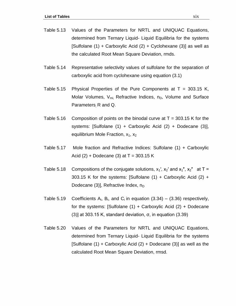
Table 5.13 Values of the Parameters for NRTL and UNIQUAC Equations,
determined from Ternary Liquid- Liquid Equilibria for the systems
[Sulfolane (1) + Carboxylic Acid (2) + Cyclohexane (3)] as well as
the calculated Root Mean Square Deviation, rmds.
Table 5.14 Representative selectivity values of sulfolane for the separation of
carboxylic acid from cyclohexane using equation (3.1)
Table 5.15 Physical Properties of the Pure Components at T = 303.15 K,
Molar Volumes, Vmi, Refractive Indices, nD, Volume and Surface
Parameters, R and Q.
Table 5.16 Composition of points on the binodal curve at T = 303.15 K for the
systems: [Sulfolane (1) + Carboxylic Acid (2) + Dodecane (3)],
equilibrium Mole Fraction, x1, x2
Table 5.17 Mole fraction and Refractive Indices: Sulfolane (1) + Carboxylic
Acid (2) + Dodecane (3) at T = 303.15 K
Table 5.18 Compositions of the conjugate solutions, x1′, x2′ and x1″, x2″ at T =
303.15 K for the systems: [Sulfolane (1) + Carboxylic Acid (2) +
Dodecane (3)], Refractive Index, nD
Table 5.19 Coefficients Ai, Bi, and Ci in equation (3.34) – (3.36) respectively,
for the systems: [Sulfolane (1) + Carboxylic Acid (2) + Dodecane
(3)] at 303.15 K, standard deviation, σ, in equation (3.39)
Table 5.20 Values of the Parameters for NRTL and UNIQUAC Equations,
determined from Ternary Liquid- Liquid Equilibria for the systems
[Sulfolane (1) + Carboxylic Acid (2) + Dodecane (3)] as well as the
calculated Root Mean Square Deviation, rmsd.
List of Tables xx
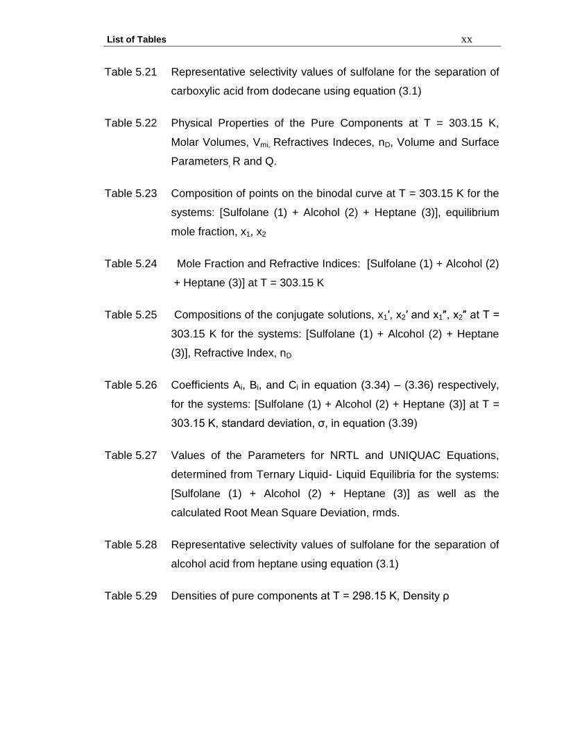
Table 5.21 Representative selectivity values of sulfolane for the separation of
carboxylic acid from dodecane using equation (3.1)
Table 5.22 Physical Properties of the Pure Components at T = 303.15 K,
Molar Volumes, Vmi, Refractives Indeces, nD, Volume and Surface
Parameters, R and Q.
Table 5.23 Composition of points on the binodal curve at T = 303.15 K for the
systems: [Sulfolane (1) + Alcohol (2) + Heptane (3)], equilibrium
mole fraction, x1, x2
Table 5.24 Mole Fraction and Refractive Indices: [Sulfolane (1) + Alcohol (2)
+ Heptane (3)] at T = 303.15 K
Table 5.25 Compositions of the conjugate solutions, x1′, x2′ and x1″, x2″ at T =
303.15 K for the systems: [Sulfolane (1) + Alcohol (2) + Heptane
(3)], Refractive Index, nD
Table 5.26 Coefficients Ai, Bi, and Ci in equation (3.34) – (3.36) respectively,
for the systems: [Sulfolane (1) + Alcohol (2) + Heptane (3)] at T =
303.15 K, standard deviation, σ, in equation (3.39)
Table 5.27 Values of the Parameters for NRTL and UNIQUAC Equations,
determined from Ternary Liquid- Liquid Equilibria for the systems:
[Sulfolane (1) + Alcohol (2) + Heptane (3)] as well as the
calculated Root Mean Square Deviation, rmds.
Table 5.28 Representative selectivity values of sulfolane for the separation of
alcohol acid from heptane using equation (3.1)
Table 5.29 Densities of pure components at T = 298.15 K, Density ρ
List of Tables xxi
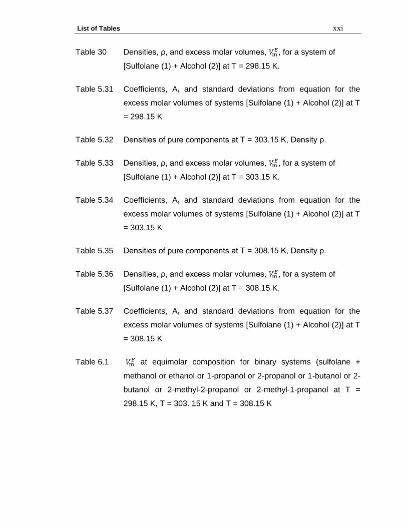
Table 30 Densities, ρ, and excess molar volumes, , for a system of
[Sulfolane (1) + Alcohol (2)] at T = 298.15 K.
Table 5.31 Coefficients, Ar and standard deviations from equation for the
excess molar volumes of systems [Sulfolane (1) + Alcohol (2)] at T
= 298.15 K
Table 5.32 Densities of pure components at T = 303.15 K, Density ρ.
Table 5.33 Densities, ρ, and excess molar volumes, , for a system of
[Sulfolane (1) + Alcohol (2)] at T = 303.15 K.
Table 5.34 Coefficients, Ar and standard deviations from equation for the
excess molar volumes of systems [Sulfolane (1) + Alcohol (2)] at T
= 303.15 K
Table 5.35 Densities of pure components at T = 308.15 K, Density ρ.
Table 5.36 Densities, ρ, and excess molar volumes, , for a system of
[Sulfolane (1) + Alcohol (2)] at T = 308.15 K.
Table 5.37 Coefficients, Ar and standard deviations from equation for the
excess molar volumes of systems [Sulfolane (1) + Alcohol (2)] at T
= 308.15 K
Table 6.1 at equimolar composition for binary systems (sulfolane +
methanol or ethanol or 1-propanol or 2-propanol or 1-butanol or 2-
butanol or 2-methyl-2-propanol or 2-methyl-1-propanol at T =
298.15 K, T = 303. 15 K and T = 308.15 K
List Figures xxii
LIST OF FIGURES
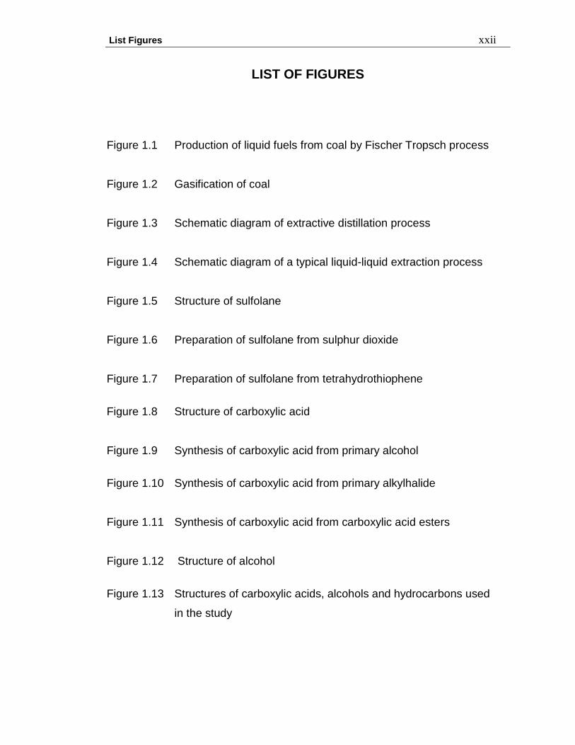
Figure 1.1 Production of liquid fuels from coal by Fischer Tropsch process
Figure 1.2 Gasification of coal
Figure 1.3 Schematic diagram of extractive distillation process
Figure 1.4 Schematic diagram of a typical liquid-liquid extraction process
Figure 1.5 Structure of sulfolane
Figure 1.6 Preparation of sulfolane from sulphur dioxide
Figure 1.7 Preparation of sulfolane from tetrahydrothiophene
Figure 1.8 Structure of carboxylic acid
Figure 1.9 Synthesis of carboxylic acid from primary alcohol
Figure 1.10 Synthesis of carboxylic acid from primary alkylhalide
Figure 1.11 Synthesis of carboxylic acid from carboxylic acid esters
Figure 1.12 Structure of alcohol
Figure 1.13 Structures of carboxylic acids, alcohols and hydrocarbons used
in the study
List Figures xxiii
Figure 3.1 Principles of liquid-liquid extraction
Figure 3.2 (a) Ternary liquid-liquid phase diagram with a small two phase
region
(b) Ternary liquid-liquid phase diagram with a large two-phase
region
Figure 3.3 Representation of Ternary liquid-liquid equilibria using a triangular
phase diagram
Figure 4.1 Binodal curve, calibration curve and tie line
Figure 4.2 Bellingham & Stanley RFM 340 Refractometer
Figure 4.3 Refraction of light when passing from medium A to medium B
Figure 4.4 Cross section of Refractometer
Figure 4.5 Anton Paar DMA 38 densimeter
Figure 4.8 Comparison of VmE results from this work with literature results
(Yang-Xin and Yi-Gui, 1998) for the mixture [sulfolane (1) +
toluene (2)].
Figure 5.1 Liquid-liquid equilibrium data for the system [sulfolane (1) + acetic
acid (2) + heptane (3)] at T = 303.15 K.
List Figures xxiv
Figure 5.2 Liquid-liquid equilibrium data for the system [sulfolane (1) +
propanoic acid (2) + heptane (3)] at T = 303.15 K.
Figure 5.3 Liquid-liquid equilibrium data for the system [sulfolane (1) +
butanoic acid (2) + heptane (3)] at T = 303.15 K.
Figure 5.4 Liquid-liquid equilibrium data for the system [sulfolane (1) +2-
methylpropanoic acid (2) + heptane (3)] at T = 303.15 K.
Figure 5.5 Liquid-liquid equilibrium data for the system [sulfolane (1) +
pentanoic acid (2) + heptane (3)] at T = 303.15 K.
Figure 5.6 Liquid-liquid equilibrium data for the system [sulfolane (1) + 3-
methylpropanoic (2) + heptane (3)] at T = 303.15 K.
Figure 5.7 Summary of Liquid-liquid equilibrium data for the following systems
at T = 303.15 K: (a) [sulfolane(1) + acetic acid (2) + heptane (3)],
(b) [sulfolane (1) + propanoic acid (2) + heptane (3)], (c)
[sulfolane(1) + butanoic acid (2) + heptane (3)], (d) [sulfolane (1) +
2-methylpropanoic acid (2) + heptane (3)], (e) [sulfolane (1) +
pentanoic acid (2) + heptanes (3)], (f) [sulfolane (1) +3-
methylbutanoic acid (2) + heptane (3)]. [Key: experimental points
(▪), experimental tie lines(x)]
Figure 5.8 Calibration curve for the system [sulfolane (1) + acetic acid (2) +
heptane (3)] at T = 303.15 K
Figure 5.9 Calibration curve for the system [sulfolane (1) + propanoic acid (2)
+ heptane (3)] at T = 303.15 K
List Figures xxv
Figure 5.10 Calibration curve for the system [sulfolane (1) + butanoic acid (2) +
heptane (3)] at T = 303.15 K
Figure 5.11 Calibration curve for the system [sulfolane (1) + 2-methylpropanoic
acid (2) + heptane (3)] at T = 303.15 K
Figure 5.12 Calibration curve for the system [sulfolane (1) + pentanoic acid (2)
+ heptane (3)] at T = 303.15 K
Figure 5.13 Calibration curve for the system [sulfolane (1) + 3-methylbutanoic
(2) + heptane (3)] at T = 303.15 K
Figure 5.14 A plot of x″2 against x′2 showing the relative solubilities of the
carboxylic acid in the sulfolane-rich and heptane- rich layer
Figure 5.15 Liquid-liquid equilibrium data for the system [sulfolane (1) + acetic
acid (2) + cyclohexane (3)] at T = 303.15 K.
Figure 5.16 Liquid-liquid equilibrium data for the system [sulfolane (1) +
propanoic acid (2) + cyclohexane (3)] at T = 303.15 K.
Figure 5.17 Liquid-liquid equilibrium data for the system [sulfolane (1) +
butanoic acid (2) + cyclohexane (3)] at T = 303.15 K.
Figure 5.18 Liquid-liquid equilibrium data for the system [sulfolane (1) + 2-
methylpropanoic acid (2) + cyclohexane (3)] at T = 303.15 K.
Figure 5.19 Liquid-liquid equilibrium data for the system [sulfolane (1) +
pentanoic acid (2) + cyclohexane (3)] at T = 303.15 K.
Figure 5.20 Liquid-liquid equilibrium data of the system [sulfolane (1) + 3-
methylpropanoic acid (2) + cyclohexane (3)] at T = 303.15 K.
List Figures xxvi
Figure 5.21 Summary of Liquid-liquid equilibrium for data for the following
systems at T = 303.15 K: (a) [sulfolane (1) + acetic acid (2) +
cyclohexane (3)], (b) [sulfolane (1) + propanoic acid (2) +
cyclohexane (3)], (c) [sulfolane(1) + butanoic acid (2) +
cyclohexane (3)], (d) [sulfolane (1) + 2-methylpropanoic acid (2) +
cyclohexane (3)], (e) [sulfolane (1) + pentanoic acid (2) +
cyclohexane(3)], (f) [sulfolane (1) +3-methylbutanoic acid (2) +
cyclohexane (3)]. [Key: experimental points (▪), experimental tie
lines(x)]
Figure 5.22 Calibration curve for the system [sulfolane (1) + acetic acid (2) +
cyclohexane (3)] at T = 303.15 K
Figure 5.23 Calibration curve for the system [sulfolane (1) + propanoic acid (2)
+ cyclohexane (3)] at T = 303. 15 K
Figure 5.24 Calibration curve for the system [sulfolane (1) + butanoic acid (2) +
cyclohexane (3)] at T = 303.15 K
Figure 5.25 Calibration curve for the system [sulfolane (1) + 2-methylpropanoic
acid (2) + cyclohexane (3)] at T = 303. 15 K
Figure 5.26 Calibration curve for the system [sulfolane (1) + pentanoic acid (2)
+ cyclohexane (3)] at T = 303. 15 K
Figure 5.27 Calibration curve for the system [sulfolane (1) + 3-methylbutanoic
acid (2) + cyclohexane (3)] at T = 303.15 K
Figure 5.28 A plot of x”2 against x‟2 showing the relative solubilities of the
carboxylic acid in the sulfolane-rich and cyclohexane-rich layer
List Figures xxvii
Figure 5.29 Liquid-liquid equilibrium data for the system [sulfolane (1) + acetic
acid (2) + dodecane (3)] at T = 303.15 K.
Figure 5.30 Liquid-liquid equilibrium data for the system [sulfolane (1) +
propanoic acid (2) + dodecane (3)] at T = 303.15 K
Figure 5.31 Liquid-liquid equilibrium data for the system [sulfolane (1) +
butanoic acid (2) + dodecane (3)] at T = 303.15 K.
Figure 5.32 Liquid-liquid equilibrium data for the system [sulfolane (1) + 2-
methylpropanoic acid (2) + dodecane (3)] at T = 303.15 K.
Figure 5.33 Liquid-liquid equilibrium data for the system [sulfolane (1) +
pentanoic acid (2) + dodecane (3)] at T = 303.15 K.
Figure 5.34 Liquid-liquid equilibrium data for the system [sulfolane (1) + 3-
methylpropanoic acid (2) + dodecane (3)] at T = 303.15 K.
Figure 5.35 Summary of Liquid-liquid equilibrium for data for the following
systems at T = 303.15 K: (a) [sulfolane(1) + acetic acid (2) +
dodecane (3)], (b) [sulfolane (1) + propanoic acid (2) + dodecane
(3)], (c) [sulfolane(1) + butanoic acid (2) + dodecane (3)], (d)
[sulfolane (1) + 2-methylpropanoic acid (2) + dodecane (3)], (e)
[sulfolane (1) + pentanoic acid (2) + dodecane (3)], (f) [sulfolane
(1) +3-methylbutanoic acid (2) + dodecane (3)]. [Key:
experimental points (▪), experimental tie lines(x)]
Figure 5.36 Calibration curve for the system [sulfolane (1) + acetic acid (2) +
dodecane (3)] at T = 303.15 K
Figure 5.37 Calibration curve for the system [sulfolane (1) + propanoic acid (2)
+ dodecane (3)] at T = 303.15 K
List Figures xxviii
Figure 5.38 Calibration curve for the system [sulfolane (1) + butanoic acid (2) +
dodecane (3)] at T = 303.15 K
Figure 5.39 Calibration curve for the system [sulfolane (1) + 2-methylpropanoic
acid (2) + dodecane (3)] at T = 303.15 K
Figure 5.40 Calibration curve for the system [sulfolane (1) + pentanoic acid (2)
+ dodecane (3)] at T = 303.15 K
Figure 5.41 Calibration curve for the system [sulfolane (1) + 3-methylbutanoic
acid (2) + dodecane (3)] at T = 303.15 K
Figure 5.42 A plot of x”2 against x‟2 showing the relative solubilities of the
carboxylic acid in the sulfolane-rich and dodecane-rich layers.
Figure 5.43 Liquid-liquid equilibrium data for the system [sulfolane (1) +
methanol (2) + heptane (3)] at T = 303.15 K.
Figure 5.44 Liquid-liquid equilibrium data for the system [sulfolane (1) +
ethanol (2) + heptane (3)] at T = 303.15 K.
Figure 5.45 Liquid-liquid equilibrium data for the system [sulfolane (1) + 1-
propanol (2) + heptane (3)] at T = 303.15 K.
Figure 5.46 Liquid-liquid equilibrium data for the system [sulfolane (1) + 2-
propanol (2) + heptane (3)] at T = 303.15 K.
Figure 5.47 Liquid-liquid equilibrium data for the system [sulfolane (1) + 1-
butanol (2) + heptane (3)] at T = 303.15 K.
Figure 5.48 Liquid-liquid equilibrium data for the system [sulfolane (1) + 2-
butanol (2) + heptane (3)] at T = 303.15 K.
List Figures xxix
Figure 5.49 Liquid-liquid equilibrium data for the system [sulfolane (1) + 2-
methyl-1-propanol (2) + heptane (3)] at T = 303.15 K.
Figure 5.50 Liquid-liquid equilibrium data for the system [sulfolane (1) + 2-
methyl-2-propanol (2) + heptane (3)] at T = 303.15 K.
Figure 5.51 Summary of Liquid-liquid equilibrium for data for the following
systems at T = 303.15 K: (a) [sulfolane(1) + methanol (2) +
heptane (3)], (b) [sulfolane + ethanol (2) + heptane (3)], (c)
[sulfolane(1) + 1-propanol (2) + heptane (3)], (d) [sulfolane (1) + 2-
propanol (2) + heptane (3]), (e) [sulfolane (1) + 1-butanol (2) +
heptane (3)], (f) [sulfolane (1) + 2-butanol (2) + heptane (3)], (g)
[sulfolane (1) + 2-methyl-1-propanol (2) + heptane (3)] and (h)
[sulfolane (1) +2-methyl-2-propanol (2) + heptane (3)]. [Key:
experimental points (▪), experimental tie lines (x)]
Figure 5.52 Calibration curve for the system [sulfolane (1) + methanol (2) +
heptane (3)] at T = 303.15 K
Figure 5.53 Calibration curve for the system [sulfolane (1) + ethanol (2) +
heptane (3)] at T = 303.15 K
Figure 5.54 Calibration curve for the system [sulfolane (1) + 1-propanol (2) +
heptane (3)] at T = 303.15 K
Figure 5.55 Calibration curve for the system [sulfolane (1) + 2-propanol (2) +
heptane (3)] at T = 303.15 K
Figure 5.56 Calibration curve for the system [sulfolane (1) + 1-butanol (2) +
heptane (3)] at T = 303.15 K
List Figures xxx
Figure 5.57 Calibration curve for the system [sulfolane (1) + 2-butanol (2) +
heptane (3)] at T = 303.15 K
Figure 5.58 Calibration curve for the system [sulfolane (1) + 2-methyl-1-
propanol (2) + heptane (3)] at T = 303.15 K
Figure 5.59 Calibration curve for the system [sulfolane (1) + 2-methyl-2-
propanol (2) + heptane (3)] at T = 303.15 K
Figure 5.60 A plot of x2″ against x2′ showing the relative solubilities of the
alcohols in the sulfolane-rich and heptane-rich layers
Figure 5.61 Plot of excess molar volume, for binary mixtures of
[sulfolane(1) + methanol (2)], [sulfolane (1) + ethanol (2)],
[sulfolane (1) + 1-propanol (2)], [sulfolane (1) +2-propanol (2)],
[sulfolane (1) +1-butanol (2)], [sulfolane (1) + 2-butanol (2)],
[sulfolane (1) +2-methyl-1-propanol (2)], [sulfolane (1) +2-methyl-2-
propanol (2)] at T = 298.15 K, as function of mole fraction
x(sulfolane)
Figure 5.62 Plot of excess molar volume, , of binary mixtures of [sulfolane(1)
+ methanol (2)], [sulfolane (1) + ethanol (2)], [sulfolane (1) + 1-
propanol (2)], [sulfolane (1) +2-propanol (2)], [sulfolane (1) +1-
butanol (2)], [sulfolane (1) + 2-butanol (2)], [sulfolane (1) +2-
methyl-1-propanol (2)], [sulfolane (1) +2-methyl-2-propanol (2)] at
T = 303.15 K, as a function of mole fraction x(sulfolane)
List Figures xxxi
Figure 5.63 Plot of excess molar volume , , for binary mixtures of
[sulfolane(1) + methanol (2)], [sulfolane (1) + ethanol (2)],
[sulfolane (1) + (1-propanol (2)], [sulfolane (1) +2-propanol (2)],
[sulfolane (1) +1-butanol (2)], [sulfolane (1) + 2-butanol (2)],
[sulfolane (1) +2-methyl-1-propanol (2)], [sulfolane (1) +2-methyl-2-
propanol (2)] at T = 308.15 K, as a function of mole fraction
x(sulfolane)
Figure 6.1 for equimolar compositions of binary systems [sulfolane +
methanol or Ethanol or 1-propanol or 2-propanol or 1- butanol or 2-
butanol or 2- methyl-2- propanol or 2-methyl -1-propanol] at T =
(298.15 K, 303.15 K and 308.15 K)
List of symbols xxxii
LIST OF SYMBOLS
T = temperature
K = kelvin
= beta coefficient for Hlavatý equation
= coefficient for Hlavatý equation
= density
Vm = molar volume
= excess molar volume
M1 = molar mass of component 1
M2 = molar mass of component 2
nD = refractive index
z = lattice coordination number
α12 = parameter in NTRL equation
ω = selectivity
λi = activity coefficient of component i
ф = segment fraction
List of symbols xxxiii
i = area fraction
ij = local area fraction of sites belonging to molecule i around sites
belonging to molecule j
= molecular configuration
δ = root mean square deviation between calculated and
experimental property
ξij = local volume fraction of molecule i in the immediate
neighbourhood of molecule j
w12 = potential energy of interaction
W12 = molar potential energy of interaction
τ = normalized parameter for symmetric systems
x1 = mole fraction of sulfolane
x2 = mole fraction of carboxylic acid (or alcohol)
x3 = mole fraction of heptane (or dodecane, or cyclohexane)
x1' = mole fraction of sulfolane in heptane (dodecane, or
cyclohexane) rich layer
x2' = mole fraction of carboxylic acid in heptane (dodecane, or
cyclohexane) rich layer
x1" = Mole fraction of sulfolane in sulfolane- rich layer
List of symbols xxxiv
x2" = Mole fraction of carboxylic acid in sulfolane-rich layer
exp = experimental value
lit = literature value
R = Volume Parameter
Q = Surface Parameter
Publications xxxv
PUBLICATIONS
1. Sithole, N.P., Redhi G.G., Liquid-liquid equilibria for mixtures of
(sulfolane + a carboxylic acid + heptane) at 303.15 K: Submitted
2. Sithole, N.P., Redhi G.G., Liquid-liquid equilibria for mixtures of
(sulfolane + a carboxylic acid + cyclohexane) at 303.15 K: In preparation
3. Sithole, N.P., Redhi G.G., Liquid-liquid equilibria for mixtures of
(sulfolane + a carboxylic acid + dodecane) at 303.15 K: In preparation
4. Sithole, N.P., Redhi G.G., Liquid-liquid equilibria for mixtures of
(sulfolane + an alcohol + heptane) at 303.15 K: In preparation
C h a p t e r 1 : I n t r o d u c t i o n 1
CHAPTER 1
INTRODUCTION
1.1 TECHNIQUE OF SEPARATION
Separation is the process of obtaining a product in pure form by removal of the
unwanted reactant/chemicals. Separation processes are essential in refineries,
in material processing, pharmaceutical and chemical industries (Letcher, 2004).
Separation processes are one of the major activities in the chemical and
petrochemical industries. It is important to use the most cost effective separation
technology to minimize waste, improve energy efficiency and increase the
efficiency of raw material used. It is vital for separation technologies to have the
potential to minimize waste and maximize productivity by separating valuable
materials that can still be re-used or sold as by-products from waste streams.
Common methods use to separate waste streams are distillation, crystallization,
adsorption, membrane processes, absorption and stripping, and liquid-liquid
extraction (Letcher, 2004).
In South Africa, Sasol is one of the companies that produce synthesis gas from
low grade coal. The products include petrol, diesel, liquefied petroleum gas and
other synthetic liquid fuels, as well as industrial pipeline gas and chemical
feedstocks. Sasol synthetic fuels produce most of South Africa‟s chemical and
polymer building blocks, including ethylene, propylene, ammonia, phenolics,
alcohols and ketones (Redhi, 1996).
C h a p t e r 1 : I n t r o d u c t i o n 2
Carboxylic acids together with many other oxygenates and hydrocarbons are
produced by Sasol using the Fischer-Tropsch process (Letcher and Reddy,
2004). Carboxylic acids are an important class of compounds with a great
number of industrial uses and applications.
The separation of carboxylic acid from mixtures of organic compound found in
Fischer-Tropsch synthesis mixtures and crude oil mixtures is an important
objective for physical chemists and for chemical engineers (Letcher and
Whitehead, 1996). In chemical industries, liquid-liquid extraction or solvent
extraction plays an important role in the separation process.
1.2 FISCHER TROPSCH CONVERSION
1.2.1 Introduction
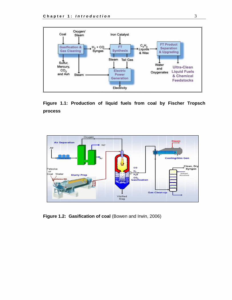
Fischer Tropsch (FT) is a catalyzed chemical reaction in which carbon monoxide
and hydrogen are converted into liquid hydrocarbons of various forms. Typical
catalysts used are based on iron and cobalt. The purpose of this process is to
produce a synthetic petroleum substitute for use as synthetic lubrication oil or
synthetic fuel (Broughton et al, 1968). Sasol is one of the petroleum industries
using this kind of synthesis, to produce a synthetic petroleum substitute, typically
from coal, natural gas or biomass, for use as synthetic lubrication oil or as
synthetic fuel for motor vehicles and some air craft engines.
C h a p t e r 1 : I n t r o d u c t i o n 3
Figure 1.1: Production of liquid fuels from coal by Fischer Tropsch
process
Figure 1.2: Gasification of coal (Bowen and Irwin, 2006)
C h a p t e r 1 : I n t r o d u c t i o n 4
1.2.2 Original Process
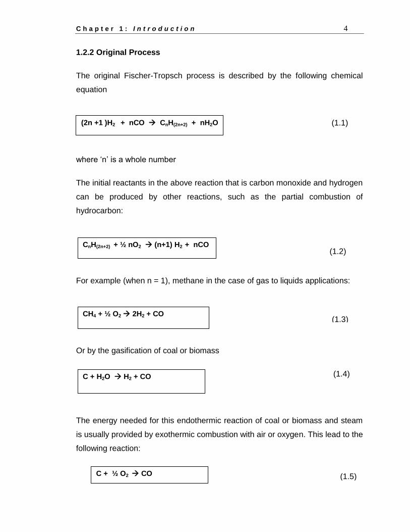
The original Fischer-Tropsch process is described by the following chemical
equation
where „n‟ is a whole number
The initial reactants in the above reaction that is carbon monoxide and hydrogen
can be produced by other reactions, such as the partial combustion of
hydrocarbon:
(1
For example (when n = 1), methane in the case of gas to liquids applications:
Or by the gasification of coal or biomass
(1.4)
The energy needed for this endothermic reaction of coal or biomass and steam
is usually provided by exothermic combustion with air or oxygen. This lead to the
following reaction:
(2n +1 )H2 + nCO CnH(2n+2) + nH2O
CnH(2n+2) + ½ nO2 (n+1) H2 + nCO
CH4 + ½ O2 2H2 + CO
C + H2O H2 + CO
C + ½ O2 CO
(1.1)
(1.2)
(1.3)
(1.5)
C h a p t e r 1 : I n t r o d u c t i o n 5
The mixture of carbon monoxide and hydrogen is called synthesis gas or
syngas. The resulting hydrocarbon products are refined to produce the desired
synthetic fuel. Carbon dioxide and carbon monoxide are generated by partial
oxidation of coal and wood-based fuels.
The utility of the process is primarily to produce fluid hydrocarbons from solid
feedstock, such as coal or solid carbon-containing wastes of various types. Non-
oxidative pyrolysis of solid material produces syngas which can be used directly
as fuel without being taken through Fischer-Tropsch transformations. If liquid
petroleum-like fuel, lubricant, or wax is required, the Fischer-Tropsch process
can be applied (Khodakov et al, 2007).
1.3 TYPICAL SEPARATION PROCESSES
1.3.1 Introduction
The design and evaluation of industrial units for separation processes require
reliable phase equilibrium data of the different mixtures involved in a given
process (Rappel and Mattedi, 2002, Mohsen-Nia et al, 2005). One way to
effectively separate a mixture of two compounds is to add a third compound
usually a polar compound such as sulfolane to the mixture. The resultant
selectivity or relative volatility of the species in the mixture can be use to design
separation procedures via liquid- liquid extraction or extractive distillation.
1.3.2 Distillation
Large scale industrial distillation applications include both batch and continuous
fractional, vacuum, azeotropic, extractive, and steam distillation (Letcher, 2004)
The most widely used industrial applications of continuous, steady-state
fractional distillation are in petroleum refineries, petrochemical and chemical
plants and natural gas processing plants.
C h a p t e r 1 : I n t r o d u c t i o n 6
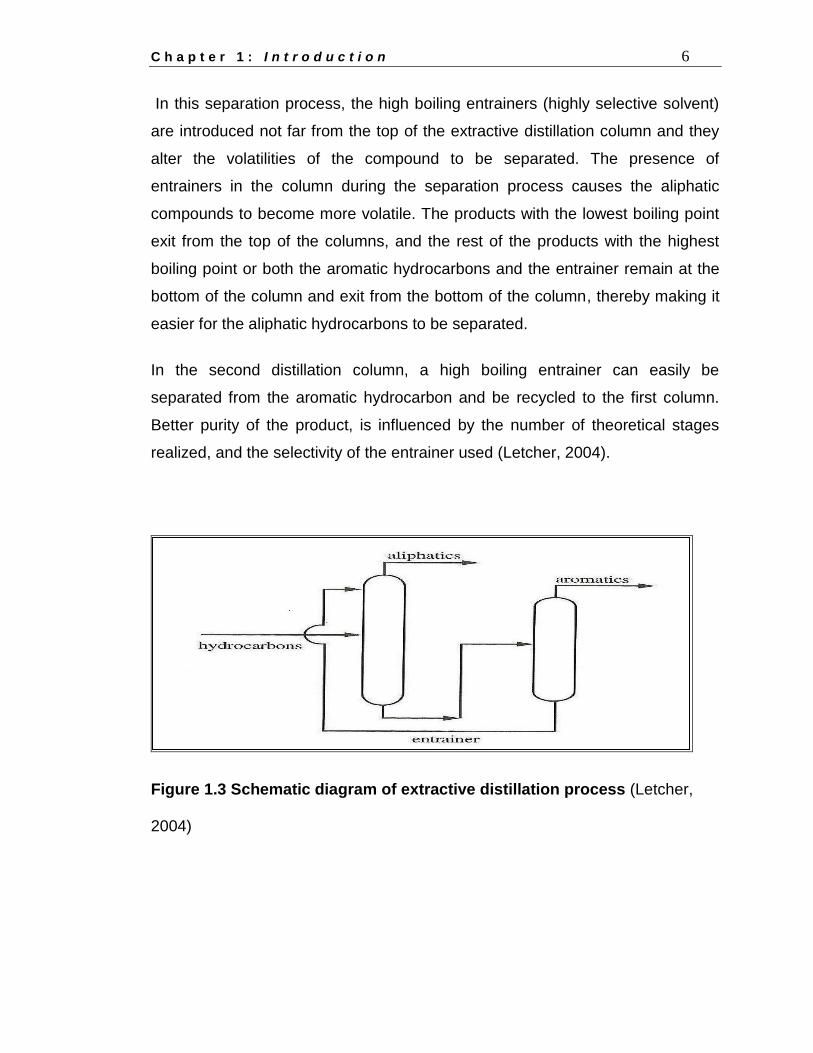
In this separation process, the high boiling entrainers (highly selective solvent)
are introduced not far from the top of the extractive distillation column and they
alter the volatilities of the compound to be separated. The presence of
entrainers in the column during the separation process causes the aliphatic
compounds to become more volatile. The products with the lowest boiling point
exit from the top of the columns, and the rest of the products with the highest
boiling point or both the aromatic hydrocarbons and the entrainer remain at the
bottom of the column and exit from the bottom of the column, thereby making it
easier for the aliphatic hydrocarbons to be separated.
In the second distillation column, a high boiling entrainer can easily be
separated from the aromatic hydrocarbon and be recycled to the first column.
Better purity of the product, is influenced by the number of theoretical stages
realized, and the selectivity of the entrainer used (Letcher, 2004).
Figure 1.3 Schematic diagram of extractive distillation process (Letcher,
2004)
C h a p t e r 1 : I n t r o d u c t i o n 7
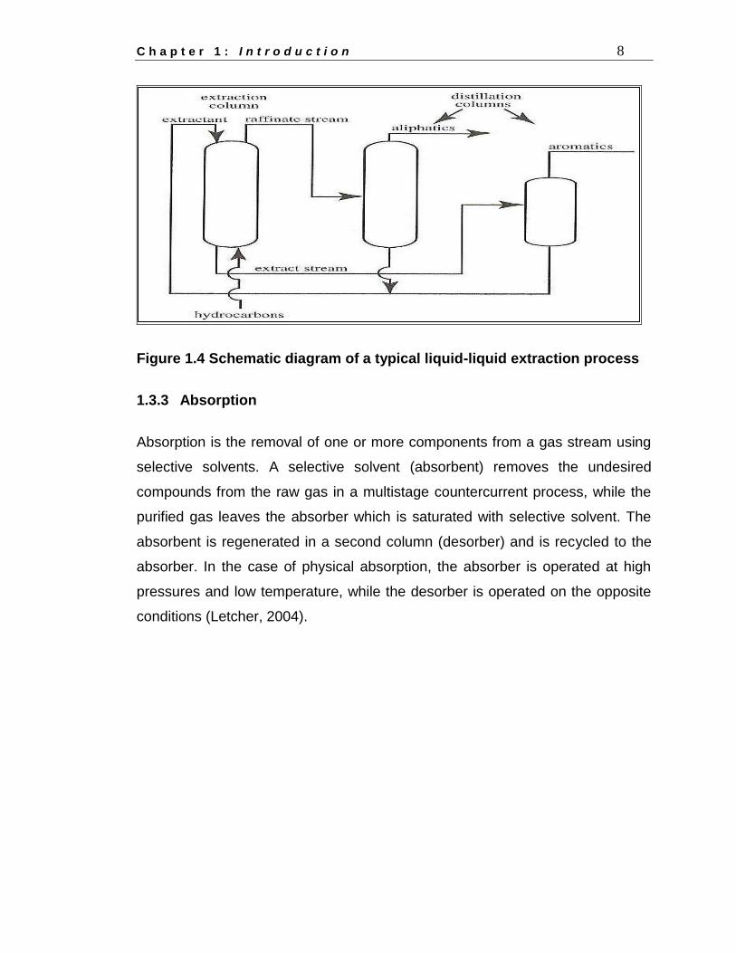
1.3.3 Liquid-liquid extraction
In liquid-liquid extraction, selective solvents are also required, which are partially
miscible with the liquid mixture to be separated. In this process, selective solvent
(extractant) is used to separate the aliphatic compounds from the aromatic
compounds in the feed stream. Distillation is used for the removal of the
selective solvent from the extract and raffinate mixture. This separation process
is used in industry for the following separation processes for separation of
systems with similar boiling points, separation of azeotropic mixtures, separation
of temperature sensitive compounds; separation of mixtures with high boiling
points and extraction of organic compounds from salt solutions (Letcher, 2004).
The selectivity, which strongly influences the number of separation stages,
together with the capacity of the solvent, strongly influences the investment cost
of a separation process. The entrainers with high selectivity and capacity are
mostly required, but unfortunately, in most cases, high selectivity values are
linked to low capacity values. The low capacity of water for example, is the
reason that in spite of its high selectivity, it is not used for the separation of
aliphatic and aromatic compounds (Letcher, 2004).
C h a p t e r 1 : I n t r o d u c t i o n 8
Figure 1.4 Schematic diagram of a typical liquid-liquid extraction process
1.3.3 Absorption
Absorption is the removal of one or more components from a gas stream using
selective solvents. A selective solvent (absorbent) removes the undesired
compounds from the raw gas in a multistage countercurrent process, while the
purified gas leaves the absorber which is saturated with selective solvent. The
absorbent is regenerated in a second column (desorber) and is recycled to the
absorber. In the case of physical absorption, the absorber is operated at high
pressures and low temperature, while the desorber is operated on the opposite
conditions (Letcher, 2004).
C h a p t e r 1 : I n t r o d u c t i o n 9
1.4 CHOICE OF SOLVENT USED IN THIS WORK FOR SOLVENT
EXTRACTION
1.4.1 Introduction
Solvent extraction depends on the physical and chemical properties of a solvent
when used for separation of complex liquid mixtures such as the recovery of
valuable products and removal of contaminants in effluent streams. The
separation potential and feasibility of solvents for commercial applicability are
dependent on the physical properties such as boiling point, thermal stability, and
viscosity, ease of recovery, toxicity and corrosive nature of the solvent.
Selectivity of the solvent is the important component in characterizing a solvent
(Letcher and Reddy, 2004).
A solvent used for solvent extraction plays a vital role in the separation process,
and the quality of the solvent used for extraction is important for the efficiency of
the desired separation process (Rappel and Mattedi, 2002). Sulfolane is one of
the most widely used in the chemical industry, as a solvent in the extraction of
hydrocarbons and aromatic hydrocarbons from naphtha feed (Mohsen-Nia and
Paikar, 2007). It has been widely used in the extraction and extractive distillation
process to recover high–purity aromatic hydrocarbons from refinery process
streams and pressurized washing processes to remove hydrogen sulphide and
carbon dioxide from synthesis gas or natural gas.
Sulfolane is a popular solvent for extraction due its good physical and chemical
properties (Senol, 2005). The quality of the solvent used in the generation and
prediction of the liquid-liquid equilibrium data for systems of interest is essential
for proper understanding of the solvent extraction process (Senol, 2005).
Sulfolane is also an industrially valuable solvent having good thermal and
hydrolytic stability, high density and high boiling point (Maciuca et al, 2008).
C h a p t e r 1 : I n t r o d u c t i o n 10
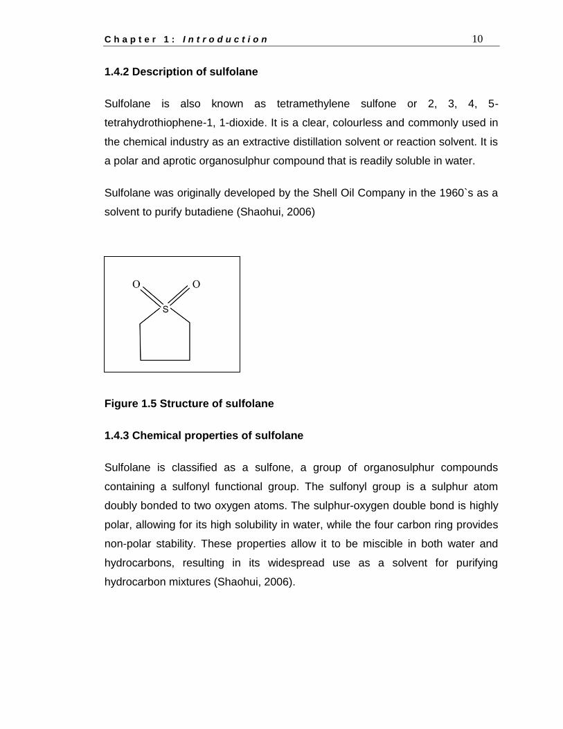
1.4.2 Description of sulfolane
Sulfolane is also known as tetramethylene sulfone or 2, 3, 4, 5-
tetrahydrothiophene-1, 1-dioxide. It is a clear, colourless and commonly used in
the chemical industry as an extractive distillation solvent or reaction solvent. It is
a polar and aprotic organosulphur compound that is readily soluble in water.
Sulfolane was originally developed by the Shell Oil Company in the 1960`s as a
solvent to purify butadiene (Shaohui, 2006)
Figure 1.5 Structure of sulfolane
1.4.3 Chemical properties of sulfolane
Sulfolane is classified as a sulfone, a group of organosulphur compounds
containing a sulfonyl functional group. The sulfonyl group is a sulphur atom
doubly bonded to two oxygen atoms. The sulphur-oxygen double bond is highly
polar, allowing for its high solubility in water, while the four carbon ring provides
non-polar stability. These properties allow it to be miscible in both water and
hydrocarbons, resulting in its widespread use as a solvent for purifying
hydrocarbon mixtures (Shaohui, 2006).
C h a p t e r 1 : I n t r o d u c t i o n 11
Sulfolane is a specialty solvent which shows the following interesting properties:
Versatility, it can be used in wide range of synthesis
High polarity and miscible with a water
Chemically and thermally stable, it has a high boiling point
Aprotic, it has a no acidic hydrogen atom
Recyclable, it is easy to recycle
It is easy to handle due to its low hazard characteristic
It is these properties that allow sulfolane to be miscible in both water and
hydrocarbons, resulting in its widespread use as a solvent for purifying
hydrocarbon mixtures (Shaohui, 2006), and is the choosen solvent for this
investigation.
1.4.4 Synthesis of sulfolene
Sulfolane can be prepared in the laboratory by the following reactions
1.4.4.1 Hydrogenation of 3-sulfolene
Industrially, sulfolane is synthesized by hydrogenation of 3-sulfolene, which is
prepared through the reaction of butadiene and sulphur dioxide (Shaohui, 2006).
C h a p t e r 1 : I n t r o d u c t i o n 12
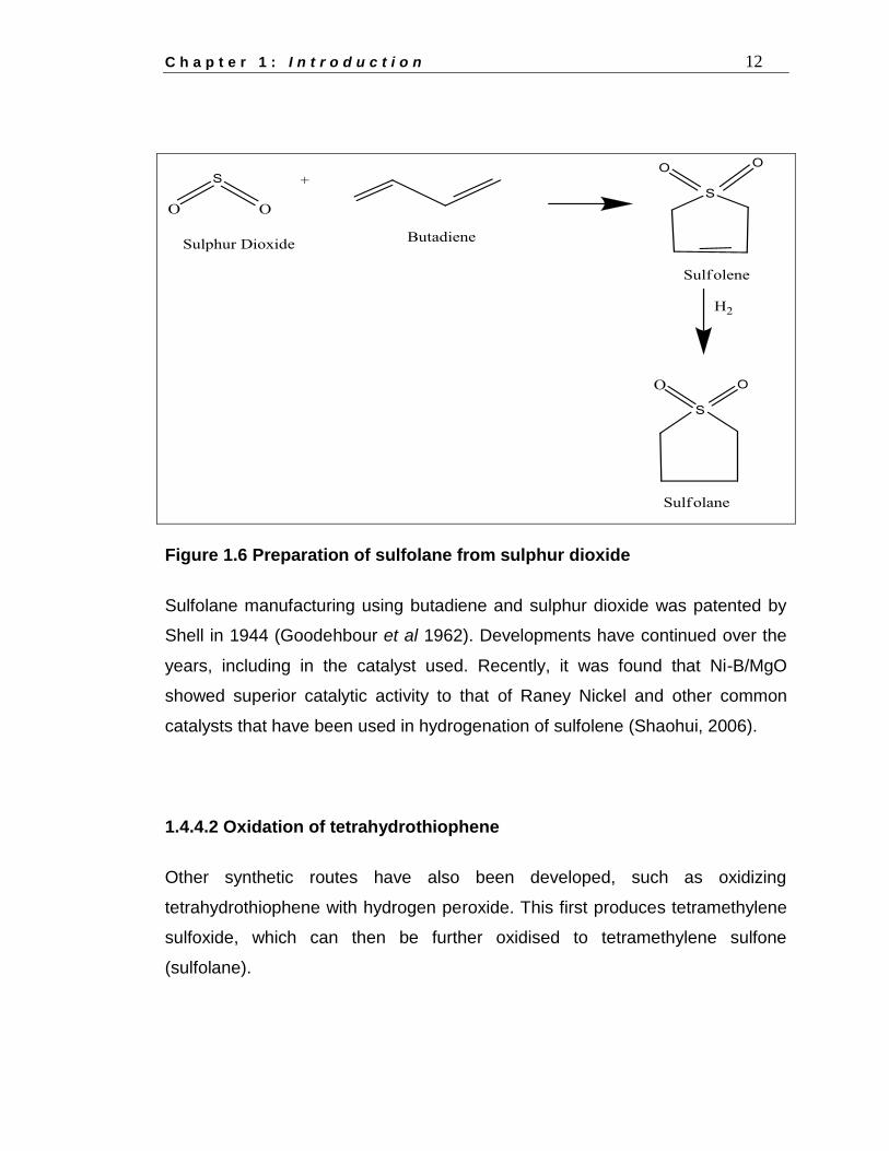
Figure 1.6 Preparation of sulfolane from sulphur dioxide
Sulfolane manufacturing using butadiene and sulphur dioxide was patented by
Shell in 1944 (Goodehbour et al 1962). Developments have continued over the
years, including in the catalyst used. Recently, it was found that Ni-B/MgO
showed superior catalytic activity to that of Raney Nickel and other common
catalysts that have been used in hydrogenation of sulfolene (Shaohui, 2006).
1.4.4.2 Oxidation of tetrahydrothiophene
Other synthetic routes have also been developed, such as oxidizing
tetrahydrothiophene with hydrogen peroxide. This first produces tetramethylene
sulfoxide, which can then be further oxidised to tetramethylene sulfone
(sulfolane).
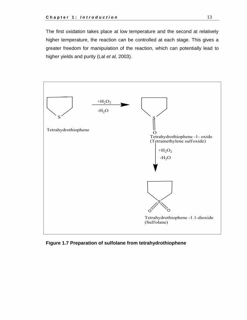
C h a p t e r 1 : I n t r o d u c t i o n 13
The first oxidation takes place at low temperature and the second at relatively
higher temperature, the reaction can be controlled at each stage. This gives a
greater freedom for manipulation of the reaction, which can potentially lead to
higher yields and purity (Lal et al, 2003).
Figure 1.7 Preparation of sulfolane from tetrahydrothiophene
C h a p t e r 1 : I n t r o d u c t i o n 14
1.4.5 Uses of sulfolane
Sulfolane is predominantly used as an extracting solvent of aromatic
hydrocarbons like benzene, toluene and xylenes from aliphatic
hydrocarbon mixtures and n-propyl alcohol and sec-butyl alcohol. It was
found to be highly effective in separating the high purity hydrocarbon
mixtures using liquid-liquid extraction. This process is still widely used
today in refineries and in the petrochemical industry (Shaohui, 2006)
It is used to purify natural gas streams and fractionation of fatty acids into
saturated and unsaturated components
It can be used in plasticize nylon, cellulose and cellulose esters to improve
flexibility and increase elongation of polymers. It can be used alone on in
combination with a co-solvent as a polymerization solvent for polyureas,
polysulfones, polysiloxanes and polyether polyols (Goodenbour et al,
1962).
Sulfolane has been tested as a solvent in lithium batteries due to its high
dielectric constant, low volatility, solubilising characteristics and aprotonic
nature.
It is used in textile industry for preparation of dyes, fabric treating prior to
dyeing and fibre treating.
Sulfolane is also an industrial solvent for purifying aromatics, it operates
at a low solvent-to-feed ratio making sulfolane units highly cost effective
Sulfolane is highly stable and can therefore be re-used many times; it
does eventually break down into acidic by-products. Some measures has
been developed to remove the by-products thereby allowing sulfolane to
be re-used and increasing the lifetime of a given supply. The methods
include vacuum and steam distillation, back extraction, adsorption and
also anion-cation exchange resin columns.
C h a p t e r 1 : I n t r o d u c t i o n 15
1.5 ORGANIC ACIDS
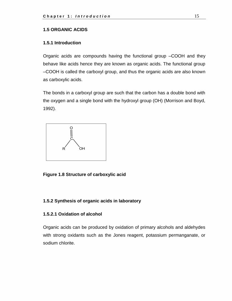
1.5.1 Introduction
Organic acids are compounds having the functional group –COOH and they
behave like acids hence they are known as organic acids. The functional group
–COOH is called the carboxyl group, and thus the organic acids are also known
as carboxylic acids.
The bonds in a carboxyl group are such that the carbon has a double bond with
the oxygen and a single bond with the hydroxyl group (OH) (Morrison and Boyd,
1992).
Figure 1.8 Structure of carboxylic acid
1.5.2 Synthesis of organic acids in laboratory
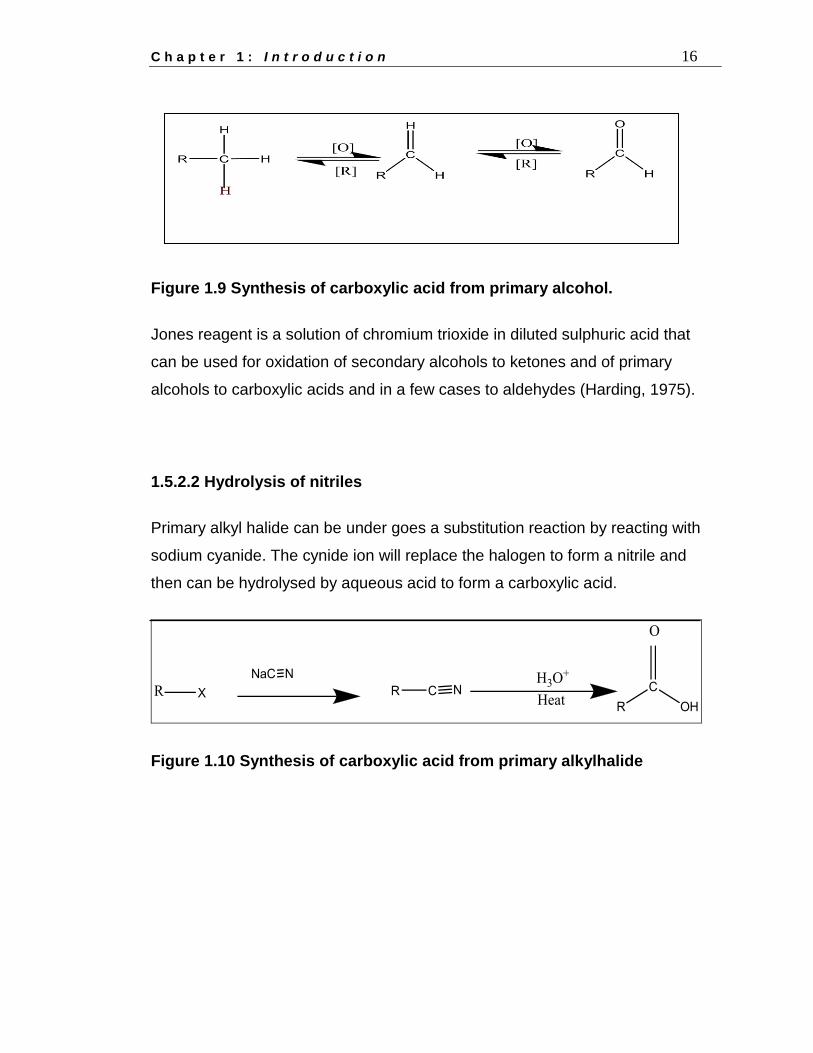
1.5.2.1 Oxidation of alcohol
Organic acids can be produced by oxidation of primary alcohols and aldehydes
with strong oxidants such as the Jones reagent, potassium permanganate, or
sodium chlorite.
C h a p t e r 1 : I n t r o d u c t i o n 16
Figure 1.9 Synthesis of carboxylic acid from primary alcohol.
Jones reagent is a solution of chromium trioxide in diluted sulphuric acid that
can be used for oxidation of secondary alcohols to ketones and of primary
alcohols to carboxylic acids and in a few cases to aldehydes (Harding, 1975).
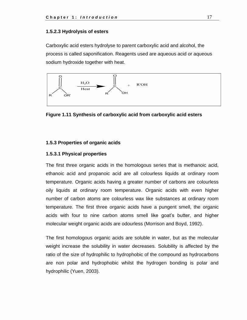
1.5.2.2 Hydrolysis of nitriles
Primary alkyl halide can be under goes a substitution reaction by reacting with
sodium cyanide. The cynide ion will replace the halogen to form a nitrile and
then can be hydrolysed by aqueous acid to form a carboxylic acid.
Figure 1.10 Synthesis of carboxylic acid from primary alkylhalide
C h a p t e r 1 : I n t r o d u c t i o n 17
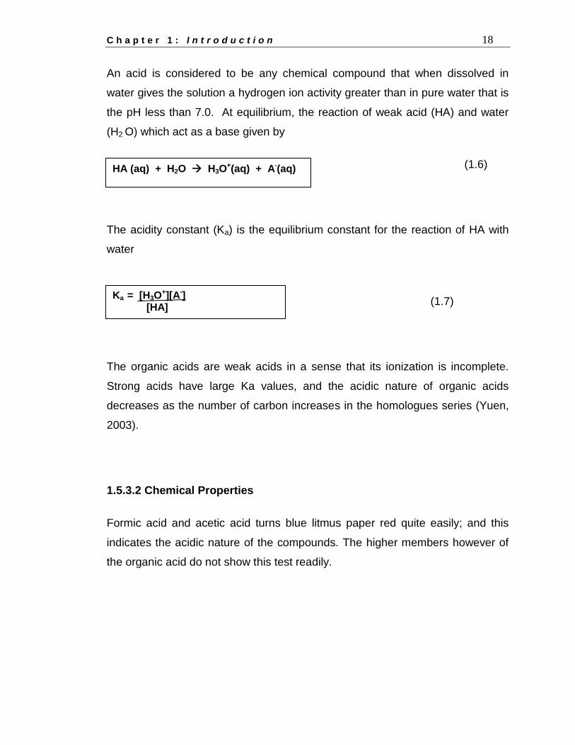
1.5.2.3 Hydrolysis of esters
Carboxylic acid esters hydrolyse to parent carboxylic acid and alcohol, the
process is called saponification. Reagents used are aqueous acid or aqueous
sodium hydroxide together with heat.
Figure 1.11 Synthesis of carboxylic acid from carboxylic acid esters
1.5.3 Properties of organic acids
1.5.3.1 Physical properties
The first three organic acids in the homologous series that is methanoic acid,
ethanoic acid and propanoic acid are all colourless liquids at ordinary room
temperature. Organic acids having a greater number of carbons are colourless
oily liquids at ordinary room temperature. Organic acids with even higher
number of carbon atoms are colourless wax like substances at ordinary room
temperature. The first three organic acids have a pungent smell, the organic
acids with four to nine carbon atoms smell like goat‟s butter, and higher
molecular weight organic acids are odourless (Morrison and Boyd, 1992).
The first homologous organic acids are soluble in water, but as the molecular
weight increase the solubility in water decreases. Solubility is affected by the
ratio of the size of hydrophilic to hydrophobic of the compound as hydrocarbons
are non polar and hydrophobic whilst the hydrogen bonding is polar and
hydrophilic (Yuen, 2003).
C h a p t e r 1 : I n t r o d u c t i o n 18
An acid is considered to be any chemical compound that when dissolved in
water gives the solution a hydrogen ion activity greater than in pure water that is
the pH less than 7.0. At equilibrium, the reaction of weak acid (HA) and water
(H2 O) which act as a base given by
(1.6)
The acidity constant (Ka) is the equilibrium constant for the reaction of HA with
water
(1.7)
The organic acids are weak acids in a sense that its ionization is incomplete.
Strong acids have large Ka values, and the acidic nature of organic acids
decreases as the number of carbon increases in the homologues series (Yuen,
2003).
1.5.3.2 Chemical Properties
Formic acid and acetic acid turns blue litmus paper red quite easily; and this
indicates the acidic nature of the compounds. The higher members however of
the organic acid do not show this test readily.
HA (aq) + H2O H3O+(aq) + A-(aq)
Ka = [H3O+][A-]
[HA]
C h a p t e r 1 : I n t r o d u c t i o n 19
Organic acids react with sodium bicarbonate to release water and carbon
dioxide. If acetic acid reacts with sodium bicarbonate, sodium ethanoate, an
ester is also formed along with water and carbon dioxide.
The reaction show below:
(1.8)
The sodium bicarbonate test is a test for the presence of the carboxyl group (-
COOH) in a compound. A positive test for carboxylic acid causes effervescence
resulting from the released of carbon dioxide.
Esters are formed when alcohols are made to react with organic acids in the
presence of concentrated sulphuric acid. The reaction below shows the reaction
of acetic acid with ethanol.
(1.9)
Ethanol and acetic acid is mixed and warmed, a few drops of concentrated
sulphuric acid is added and a sweet smell will emanate from the reaction. The
sweet smell is the smell of the ester, ethyl ethanoate.
1.5.4 Applications of organic acids
Simple organic acids like methanoic and ethanoic acids are used for oil
and gas cell stimulation treatments
Acetic acid is also used in some food items for example vinegar and it is
used by medical industries for synthesis of asprin.
CH3COOH + NaHCO3 CH3COONa + H2O + CO2
CH3COOH + CH3CH2OH CH3COOCH2CH3 + H2O
C h a p t e r 1 : I n t r o d u c t i o n 20
Acetic acid is used for coagulation of latex; it is needed when rubber is
made from latex in the rubber industry.
Acetic acid is used for making cellulose acetate, which is an important
starting material for making artificial fibres.
Propanoic acid inhibits the growth of the mold and some bacteria, and
as a result it is used as a preservative for both animal feed and food for
human consumption (Bertleff et al, 2003).
Propanoic acid is useful as an intermediate in the production of other
chemicals, especially polymers, for example cellulose-acetate propionate
is a useful thermoplastic used to make pesticides and pharmaceuticals.
Esters of propanoic acid have fruit-like odours and are sometimes used
as a solvents or artificial flavourings (Bertleff et al, 2003).
Propanoic acid and its calcium, sodium and potassium salts are widely
used throughout the food industry as preservatives (Ahmad and Othman,
2010)
Propanoic acid as a preservative extends the shelf life of food products
by inhibiting the growth of moulds and some bacteria (Ahmad and
Othman, 2010)
Butanoic acid is used in the preparation of various butanoate esters, low
molecular weight esters of butanoic acid such as methyl butanaote, have
mostly pleasant aromas or taste, and they are used as food and perfume
additives.
Pentanoic acid is primarily used to synthesis esters; volatile esters of
pentanoic acid tend to have pleasant odours and are used in perfumes
and cosmetics. Ethyl valerate and pentyl valerate are used as food
additives because of their flavours.
2-Methylbutanoic acid is used for synthetic lubricants and is also used
as a chemical intermediate for plasticizers, pharmaceuticals, metallic
salts and vinyl stabilizers.
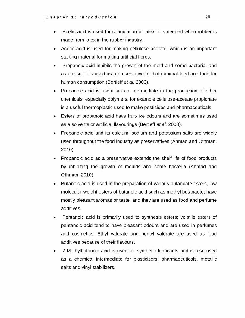
C h a p t e r 1 : I n t r o d u c t i o n 21
1.6 ALCOHOLS
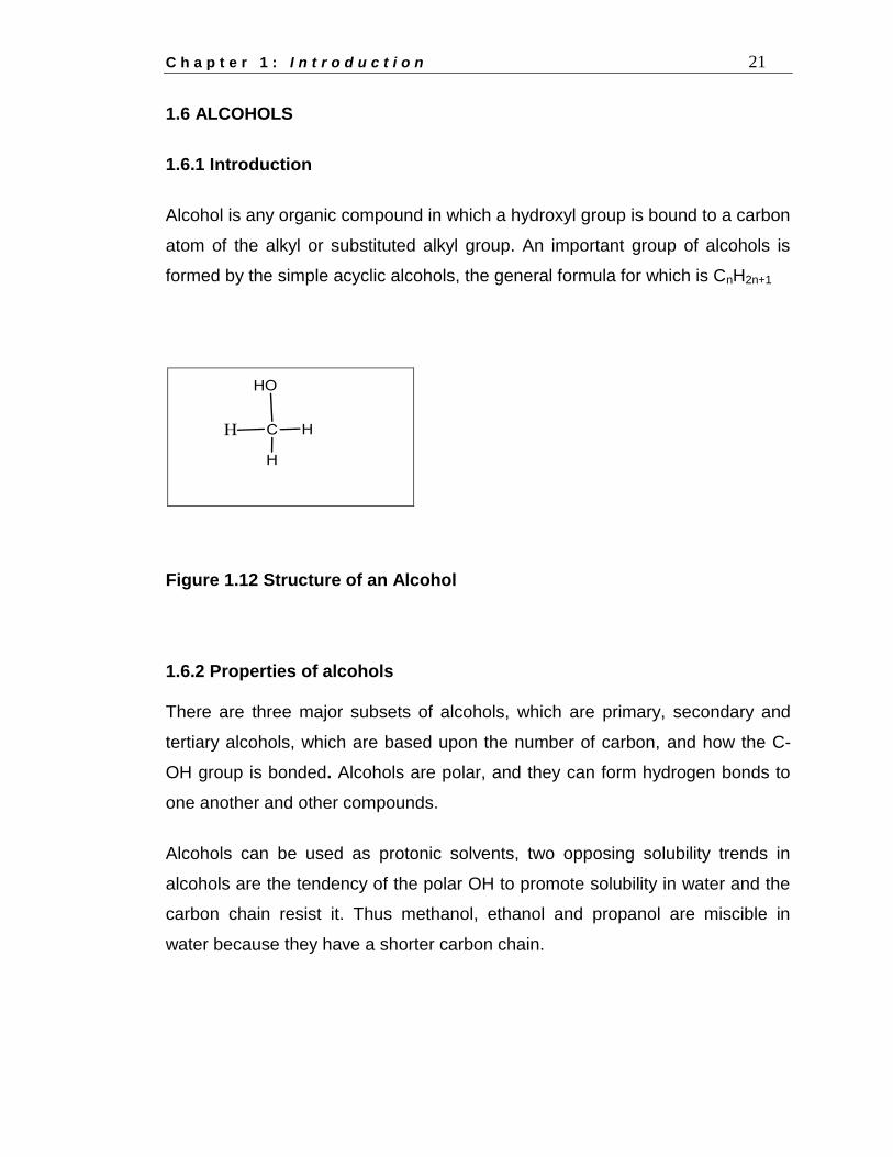
1.6.1 Introduction
Alcohol is any organic compound in which a hydroxyl group is bound to a carbon
atom of the alkyl or substituted alkyl group. An important group of alcohols is
formed by the simple acyclic alcohols, the general formula for which is CnH2n+1
Figure 1.12 Structure of an Alcohol
1.6.2 Properties of alcohols
There are three major subsets of alcohols, which are primary, secondary and
tertiary alcohols, which are based upon the number of carbon, and how the C-
OH group is bonded. Alcohols are polar, and they can form hydrogen bonds to
one another and other compounds.
Alcohols can be used as protonic solvents, two opposing solubility trends in
alcohols are the tendency of the polar OH to promote solubility in water and the
carbon chain resist it. Thus methanol, ethanol and propanol are miscible in
water because they have a shorter carbon chain.
C h a p t e r 1 : I n t r o d u c t i o n 22
Butanol is moderately soluble in water, and alcohols that have five and more
carbon are effectively insoluble in water. All simple alcohols are miscible in
organic solvents. Alcohols have an odour that is often described as biting and as
hanging in the nasal passages.
1.6.3 Applications of alcohol
Ethanol is the only alcohol than can be used as an alcoholic beverage
and has been consumed by humans since pre-historic times
Methanol and ethanol can also be used as the alcohol fuel, the fuel
performance can be increased in force induction internal combustion by
injecting alcohol into the air intake, after the turbocharger or supercharger
has pressurized the air.
Alcohols can also be used in chemical industries as reagents or solvents
because they of its low toxicity and ability to dissolve non polar
substances.
Ethanol can be used as a solvent in medical drugs. It canalso be used as
an antiseptic to disinfect the skin before injections are given along with
iodine.
Alcohol gels has been common as hand sanitizers
Ethanol is used as the preservative for specimens
Ethanol-based soaps are becoming common in restaurants and are
convenient because they require less drying due to the volatility of the
compound.
In organic synthesis alcohols serves as versatile intermediates.
C h a p t e r 1 : I n t r o d u c t i o n 23
1.7 AREA OF RESEARCH COVERED IN THIS WORK
This project involves an investigation into the feasibility of separation of
carboxylic acids from hydrocarbons including a cyloalkane, using sulfolane as a
solvent for extraction. Solvents for extraction should have a high selectivity for
one of the components, high capacity, capacity to form two phases at
reasonable temperatures, capability of rapid phase separation, be non-
corrosive, non-reactive and show good thermal stability.
In the first part of this work, the effectiveness of solvent extraction by sulfolane
was investigated for ternary systems at T = 303.15 K. The ternary systems
consist of (sulfolane + carboxylic acid + hydrocarbon), (sulfolane + carboxylic
acid + cycloalkane) and (sulfolane + alcohol + hydrocarbon).
Liquid- liquid equilibria data at T = 303.15 K were obtained for the following
systems:
Sulfolane + acetic acid or propanoic acid or butanoic acid or 2-
methylpropanoic acid or pentanoic acid or 3-methylbutanoic acid +
heptane
Sulfolane + acetic acid or propanoic acid or butanoic acid 2-
methylpropanoic acid or or pentanoic acid or 3-methylbutanoic acid +
cyclohexane.
Sulfolane + acetic acid or propanoic acid or butanoic acid 2-
methylpropanoic acid or or pentanoic acid or 3-methylbutanoic acid +
dodecane.
Sulfolane + methanol or ethanol or 1- propanol or 2-propanol or 1-butanol
or 2-butanol or 2-methyl-1-propanol or 2-methyl-2-propanol + heptane.
C h a p t e r 1 : I n t r o d u c t i o n 24
The purpose of this project is develop a economically viable separation of
carboxylic acids or alcohols from hydrocarbons using sulfolane serves two
purposes, polluted aqueous streams can be cleaned up and high valued
chemicals can be produced relatively cheaply. This in turn will save South Africa
valuable foreign exchange as many of these compounds are imported.
The liquid-liquid equilibria work in this project was aimed at finding the following
effect of the ternary mixtures [sulfolane (1) + a carboxylic acid (2) or alcohol (2)
+ hydrocarbon (3)] on the phase equilibria
Increasing the carbon chain length of carboxylic acid
Increasing the carbon chain length of the hydrocarbon
The second part of this work is the fitting of the binodal models to the
experimental binodal data determined. The modified Hlavatý, beta (β) and log γ
equations will be fitted to the experimental binodal data. The NRTL (Non-
Random, Two Liquid) and UNIQUAC Universal Quasichemical) model would be
used to correlate the experimental tie-lines and calculate the phase
compositions of the ternary systems.
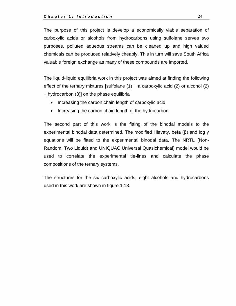
The structures for the six carboxylic acids, eight alcohols and hydrocarbons
used in this work are shown in figure 1.13.
C h a p t e r 1 : I n t r o d u c t i o n 25
Figure 1.13 Structures of carboxylic acids, alcohols and hydrocarbons
used in the study
The third part of this work involves investigating of the excess molar volumes of
the binary mixtures (sulfolane + an alcohol) T = 298.15 K, T = 303.15 K and T =
308.15 K. The sulfolane mixtures were [sulfolane (1) + methanol or ethanol or 1-
propanol or 2- propanol or 1-butanol or 2-butanol or 2-methyl-1-propanol or 2-
methyl-2-propano (2)]. Excess molar volume data is a useful parameter in the
design of the technological separation processes for the components, and can
be used to predict vapour liquid equilibria using appropriate equation of state
models. Redlich–Kister equation was used to correlate the excess molar volume
data obtained.
CH3COOH acetic acid
CH3CH2COOH propanoic acid
CH3CH2CH2COOH butanoic acid
(CH3)CHCOOH 2-methylpropanoic acid
CH3CH2CH2CH2COOH pentanoic acid
(CH3)2CHCH2COOH 3-methylbutanoic acid
CH3OH methanol
CH3CH2OH ethanol
CH3CH2CH2OH 1-propanol
CH3CH(OH)CH3 2-propanol
CH3CH2CH2CH2OH 1-butanol
CH3CH(CH3)CH2(OH) 2-methyl-1-propanol
CH3CH(OH)(CH3)CH3 2-methyl-2-propanol
CH3(CH2)5CH3 heptane
C7H14 cyclohexane
C12H26 dodecane
C h a p t e r 2 : L i t e r a t u r e R e v i e w 26
CHAPTER 2
LITERATURE REVIEW
2.1 LIQUID-LIQUID EQUILIBRIUM FOR TERNARY MIXTURES
Solvent extraction is a major technique and its operation is based entirely on
limited liquid miscibility and the distribution of solutes between two liquid phases.
The separation of two components in solution is achieved by the addition of the
third component, that is the third liquid which is added to the solution mixture to
bring about the extraction. This solvent takes up part of the components of the
original solution and forms an immiscible layer composed of the remainder of
the original solution plus some of the solvent (Redhi, 2003). Sulfolane is popular
solvent for extraction due its physical and chemical properties.
Lee and Kim (1995) presented liquid-liquid equilibrium data for the systems
(sulfolane + octane + benzene), (sulfolane + octane + toluene) and (sulfolane +
octane + p-xylene) at T = 298.15 K, T = 308.15 K and T = 318.15 K. It was
reported that the size of the two phase region decrease with an increase in the
temperature. The tie line data were satisfactory correlated by the Othmer and
Tobias method, and the experimental data were compared to the values
calculated by the UNIQUAC and NRTL models. It was concluded that although
good quantitative agreement was obtained with both these models, the NRTL
model values were found to be substantially better than UNIQUAC model
values.
C h a p t e r 2 : L i t e r a t u r e R e v i e w 27
Chen-Feng and Wen-Churng (1999) presented the liquid-liquid equilibria of
alkane C10/C12/C14) + octylbenzene + sulfolane) at T = 323.15 K, T = 348.15 K
and T = 373.15 K. The addition of octylbenzene to sulfolane was found to
increase the solubility of alkanes in the order of n-decane > n-dodecane > n-
tetradecane. It was concluded that the higher the temperature, the larger the
distribution coefficient value. An increase in solvent capacity (distribution
coefficient) of sulfolane leads to a decrease in its selectivity, therefore in-order to
choose the optimum values of the selectivity and solvent capacity, a
compromise between the two parameters must be achieved by adjusting the
temperature or adding a second component like water to the solvent.
Chen-Feng and Wen-Churng (1999) studied the ternary liquid-liquid equilibria of
alkane ((C10/C11/C12/C14) + 1.4 disopropylbenzene + sulfolane) at T = 322.15
K, T = 348.15 K and T = 373.15 K. The addition of 1.4, diisopropylbenzene to
sulfolane was found to increase the solubility of alkanes in the order of n-decane
> n-dodecane > n-tetradecane and the relative mutual solubility of 1.4-
diisopropylbenzene is higher in (n-decane + sulfolane) than in the (n-dodecane
+ sulfolane) or (n-tetradecane + sulfolane) mixtures. The size of the two phase
region was found to decrease with an increase in temperature, and from the
selectivity data, it can be concluded that the separation of 1.4-
diisopropylbenzene from n-decane, n-dodecane or n-tetradecane is feasible with
sulfolane as a solvent.
Chen et al., (2000) studied the liquid-liquid equilibrium data of six ternary
systems: (n-hexane + benzene + sulfolane), (n-hexane + toluene + sulfolane, n-
hexane + xylene + sulfolane), (n-octane + benzene + sulfolane, n-octane +
toluene + xylene + sulfolane), three quaternary systems: (n-hexane + n-octane +
benzene + sulfolane), (n-hexane + benzene + toluene + sulfolane, n-octane +
toluene + xylene + sulfolane), one quinary system: (n-hexane + n-octane +
benzene + toluene + sulfolane).
C h a p t e r 2 : L i t e r a t u r e R e v i e w 28
Chen et al., found that NRTL and UNIQUAC parameters between n-hexane and
n-octane, benzene and toluene, benzene and xylene, toluene and xylene are
suggested to be zero. The results from the quarternary and quinary systems
showed RMDS are < 0.01. The maximum deviation is 0.018 for the mole fraction
of sulfolane in the system (n-hexane + n-octane + benzene + sulfolane).
Letcher and Redhi (2001) presented the liquid-liquid equilibrium data for
(acetonitrile + acetic acid, or propanoic acid, or butanoic acid, or 2-
methylpropanoic acid, or pentanoic acid, or 3-methylbutanoic acid +
cyclohexane) at T = 298.15 K. The relative mutual solubility of each of the
carboxylic acids was higher in the acetonitrile than in the hydrocarbon layer. The
influence of 3-methylbutanoic acid, pentanoic acid, 2-methylpropanoic acid and
butanoic acid on the solubility of the hydrocarbon in acetonitrile was greater than
that of acetic acid and propanoic acid. The separation of carboxylic acid from
the cyclohexane by extraction with acetonitrile was feasible.
Wen-Churng and Nein-Hsin (2002) presented equilibrium tie line data at T =
323.15 K, T = 348.15 K and T = 373.15 K for the ternary liquid- liquid equilibria
of octane + (benzene or toluene or m-xylene + sulfolane) systems. The mutual
solubility of benzene was higher than that of toluene or m-xylene in (octane +
sulfolane) mix. Correlation of tie line data showed that calculated values based
on the NRTL were found to be better than those based on UNIQUAC equation.
Rappell et al., (2002) studied the ternary systems of (sulfolane + p-xylene +
cyclohexane), (sulfolane + p-xylene + n-hexane) and (sulfolane + toluene + n-
hexane) at T = 308.15 K and T = 323.15 K. The systems were compared at
different temperatures and the results showed that the two-phase region was
enlarged as the temperature was increased, indicating that at higher
temperature, sulfolane is more selective solvent for aromatic compounds. The
experimental data was better fitted with the NRTL than the UNIQUAC model.
C h a p t e r 2 : L i t e r a t u r e R e v i e w 29
Ahmad et al., (2004) presented interaction parameters for multi-component
aromatic extraction with sulfolane. Activity coefficient models were used to
predict the behaviour of ternary data of systems at different temperatures. The
parameter estimation procedure was modified to estimate the parameters
simultaneously for different systems involving common pairs that were used for
parameter estimation. It was reported that the results of separate estimation
showed that the binary interaction parameters for the same pairs are different for
different systems. The objective function was modified to estimate the binary
interaction parameters using three systems with common pairs simultaneously.
Mohsen-Nia et al., (2005) studied the ternary mixtures of (solvent + aromatic
hydrocarbon + alkane) at different temperatures from T = 298.15 K to T =
313.15 K. The aromatic hydrocarbon was toluene or m-xylene and the alkane
was n-heptane or n-octane or cyclohexane and the solvent was sulfolane or
dimethyl sulfoxide or ethylene carbonate. It was reported that the size of the two
phase region decreased with increase in temperature.
The selectivity and distribution coefficient of the used solvents were compared in
this study. It was also reported that in extraction of aromatics from non
aromatics, the solvent with higher selectivity and distribution coefficient, was
preferred, and based on calculated selectivity and distribution coefficient
indicated the superiority of ethylene carbonate and dimethyl sulfoxide. It was
concluded based on the very strong and bad odour, as well as recovery
difficulties of dimethyl sulfoxide, ethylene carbonate was considered a better
solvent than dimethyl sulfoxide.
Im et al., (2006) studied the liquid- liquid equilibrium of the binary of sulfolane
and branched cycloalkanes (methylcyclopentane, methylcyclohexane, and
ethylcyclohexane) over the temperature range around T = 300 K to T = 460 K.
C h a p t e r 2 : L i t e r a t u r e R e v i e w 30
The compositions of both branched cycloalkane-rich and sulfolane-rich phases
were analyzed by on-line gas chromatography. The quantitative description of
liquid-liquid equilibria of industrial interest containing sulfolane and branched
cycloalkanes was gathered to accurately simulate and optimize the extractive
distillation units, where these systems were involved.
Mohsen-Nia and Paikar (2007) presented the liquid-liquid equilibrium data for
ternary and quaternary systems containing (n-hexane, toluene, m-xylene,
propanol, sulfolane and water) were at T = 303.15 K. The efficiency of extraction
of toluene or m-xylene from n-hexane by using sulfolane as the pure-solvent and
(sulfolane + propanol) or (sulfolane + water) as the mixed-solvents is evaluated
by comparison of the selectivity factors and distribution coefficients. It was
concluded that the extraction of toluene an m-xylene from n-hexane the mixed-
solvent (sulfolane + propanol) has lower selectivity factor and higher distribution
coefficient than the pure solvent sulfolane at T = 303.15 K.
Santiago and Aznar (2007) studied the liquid- liquid data for three quaternary
systems containing (sulfolane, nonane + undecane + benzene + sulfolane),
(nonane + undecane + toluene + sulfolane), and (nonane + undecane + m-
xylene + sulfolane) at T = 298.15 K and T = 313.15 K and ambient pressure.
The size of the two-phase region was reported to decrease with an increase in
temperature. The effect was mostly observed in the systems containing the m-
xylene. It was observed that toluene, benzene and m-xylene were more soluble
in the hydrocarbon than in the sulfolane. The slope of the tie lines showed that
toluene, benzene and m-xylene are soluble in hydrocarbon-rich mixture than in
sulfolane-rich mixture. The solubility effect was reported to be reflected in the
size of the two-phase region, which increased slightly in order benzene >
toluene > m-xylene at the same temperature. It was concluded that the effect of
temperature was very small on the liquid –liquid equilibrium data.
C h a p t e r 2 : L i t e r a t u r e R e v i e w 31
Santiago and Aznar (2007) the presented the liquid- liquid data three quinary
mixtures (nonane + undecane + benzene + toluene + sulfolane), (nonane +
undecane + benzene +m-xylene + sulfolane) and (nonane + undecane + toluene
+ m-xylene + sulfolane) at T = 298.15 K and T= 313.15 K and ambient pressure.
Liquid–liquid equilibrium data of the three quinary systems, (nonane + undecane
+ benzene or toluene or m-xylene) was investigated. It was reported that the
size of the two-phase region decreased with an increase in temperature. This
effect was observed to be stronger in the systems containing m-xylene. The
data also showed that toluene, benzene and m-xylene were more soluble in the
aliphatic-rich phase than in sulfolane-rich phase. This solubility effect was
reflected in the size of the two-phase region, which increased slightly in the
order benzene > toluene > m-xylene, at the same temperature.
Awwad et al., (2008) presented the liquid-liquid equilibria for pseudo-ternary
systems for [sulfolane + 2-ethyoxyethanol (1) + octane (2) + toluene (3)] at T =
293.15 K. It was reported the solvent (sulfolane + 0.75% ethoxyethanol)
showed higher capacity for toluene compared to pure sulfolane and for that
reason it could be used for higher recovery of aromatics at lower solvent to feed
ratios and temperatures. It was concluded from the selectivity values that the
separation of toluene from octane by extraction with (sulfolane + mass % 2-
ethyoxyethanol) was feasible. The comparison between experimental selectivity
data of (sulfolane + mass % 2-ethyoxyethanol) with that of (sulfolane + 2-
methoxyethanol) for the extraction of toluene from (toluene + octane) mixture at
T = 293.15 K was more efficient using (sulfolane + mass % 2-methoxyethanol).
C h a p t e r 2 : L i t e r a t u r e R e v i e w 32
Mohmoudi et al., (2010) studied the liquid-liquid equilibrium properties for the
binary systems containing (n-formoylmorpholine + benzene + n-hexane),
(sulfolane + benzene + n-hexane) and quaternary mixed solvent system
(sulfolane + N-formolymorphiline + benzene + n-hexane) measured at
temperature ranging from T = 298.15 K to T = 318.15 K and at atmospheric
pressure. The experimental distribution coefficients and selectivity factors were
presented to evaluate the efficiency of the solvents for extraction of benzene
from n-hexane. The liquid-liquid equilibria results reported indicated that
increasing temperature decreased the selectivity for all solvents. It was
concluded from the result that sulfolane has highest selectivity and n-
formoylmorpholine has the highest distribution coefficient whilst the mixed
solvent (sulfolane + n-formoylmorpholine has higher selectivity factor than n-
formoylmorpholine and higher distribution coefficient than sulfolane. It was
concluded that all solvents are feasible for separation, but selection of the best
solvent depends on the most economically viable.
2.2 EXCESS MOLAR VOLUMES MIXTURES
There is no volume change upon mixing two liquids to form a thermodynamically
ideal solution at constant temperature and pressure, but a volume change may
occur when two real liquids are mixed (Battino, 1971). The volume change on
mixing of binary liquid mixtures, , at constant pressure and temperature is of
interest to chemists and chemical engineers, and is an indicator of the non-
idealities present in real mixtures. It is important to thermochemists because it
serves as a sensitive indicator for the applicability of liquid mixtures (Redhi,
2003).
C h a p t e r 2 : L i t e r a t u r e R e v i e w 33
Benoit and Charbonneau (1969) presented molar excess free energies for the
systems of (sulfolane + benzene) and (sulfolane + dichloromethane) were
calculated from static vapour pressure measurement at T = 303.15 K.
Refractive indexes, excess partial molar volumes of mixing and enthalpies of
mixing at infinite dilution of benzene and dichloromethane were also determined.
The excess Gibbs free energy was observed to be negative and the heat of
solution at infinite dilution of dichloromethane was exothermic. It was concluded
that the complex-forming interactions between the solvent and molecules and
such complexes are known to exist in other binary systems of dichloromethane
with a proton acceptor.
Yang-Xin and Yi-Gui (1998) presented the excess molar volume data on mixing
for binary mixtures of sulfolane with toluene, o-xylene, m-xylene, p-xylene,
ethylbenzene and 1,2,4-trimethylbenzene at T = 298.15 K. It was found that all
mixtures exhibited negative excess volumes over the entire mole fraction range
for all binary systems. It was reported that the negative excess molar volumes
were due to the expansion in volume due to mutual loss of dipolar association
and the difference in size of and shape of the component molecules and that
contraction in volume comes from the dipole-induced and dipole-dipole
interactions and donor acceptor interactions between unlike molecules. The
molar volumes for equimolar mixtures were found to vary in the order of toluene
> p-xylene > m-xylene > ethylbenzene > o-xylene > 1,2,4-trimethylbenzene.
Letcher et al., (2000) studied the excess molar volumes and excess molar
enthalpies were measured as a function of mole fraction at T= 303.15 K and
atmospheric pressure for each of the mixtures (1-heptyne, or 1-octyne +
sulfolane). The excess molar volumes were also measured for mixtures of (1-
hexyne + sulfolane).
C h a p t e r 2 : L i t e r a t u r e R e v i e w 34
The results were compared in an attempt to investigate the interactions between
the highly polar sulfolane molecule and the terminal proton of the alkynes.
The excess molar volumes for all the mixtures of (1-alkyne + sulfolane)
measured were very large, negative and slightly asymmetrical in form. The
increase in the molar excess volume was in the sequence 1-hexyne >1-heptyne
> 1-octyne
Yang-Xin et al., (2000) presented data on two binary mixtures of (water +
sulfolane) and (water + tetraethylene glycol). The excess molar volumes for both
binary mixtures were negative and it was shifted towards the water-rich region
for the (water + sulfolane) and (water + tetra-ethylene glycol) systems. Excess
molar volumes for aqueous tetraethylene glycol solutions are smaller than those
for the other systems of sulfolane and water. This effect was explained as
follows: the increase in the order of the system is due to the formation of
hydrogen bonds between water and tetra-ethylene glycol molecules.
Yang et al., (2004) presented densities and viscosities of the binary systems of
(sulfolane + ethylbenzene, sulfolane + p-xylene) at T = 303.1 K to T = 353.15 K
and at atmospheric pressure. It was reported that the excess molar volume of
the two mixtures exhibited negative excess molar volumes on the entire
composition range for the two systems. It was also found that excess molar
volumes and viscosity deviation showed a systematic change with increasing
temperature.
Wang et al., (2004) presented the excess molar volumes of (cyclohexanone +
benzene, or toluene, or ethylbenzene, or styrene), obtained from the densities
over the composition range at temperature T = ( 293.15 K, 303.15 K, 313.15 K,
323.15 K, 333.15 K, 343.15 K and 353.15 K) and atmospheric pressure.
C h a p t e r 2 : L i t e r a t u r e R e v i e w 35
It was reported that the excess molar volumes had shifted in a regular way with
the increasing temperature from T = 293.15 K to 313.15 K.
In each system, a slight decrease in the excess molar volumes over the whole
mole fraction range was noticeable with increasing temperature. It was
concluded that by comparison of the minimum values of excess molar volumes
for three mixtures containing an aromatic hydrocarbon at the same temperature,
styrene was the most favourable one to form close packing with cylohexanone.
Chen et al., (2005) presented viscosities and densities for binary mixtures of n-
methylpiperazine with methanol, ethanol, n-propanol, isopropanol, n-butanol and
isobutanol at T = 293.15 K, T = 298.15 K and T = 303.15 K and atmospheric
pressure. It was reported that all the investigated systems exhibited very large
positive values of viscosity deviation, and excess Gibbs energy and excess
molar volumes were negative over the entire composition range. The deviations
were attributed to the strong cross association between the alkonol and n-
methylpiperazine molecules through the hydrogen bond of O-H-N. It was also
reported the temperature had a significant effect on viscosity deviation, and
relatively slight effect on the excess molar volumes and excess Gibbs energy.
Šerbanović et al., (2006) presented the four binary mixtures of (methanol +
benzene), (ethanol + benzene), (methanol + chlorobenzene) and (ethanol +
chlorobenzene) at six different temperatures, T= (288.15 K, 293.15 K, 303.15 K,
308.15 K and 313.15 K). It was reported that the results were analysed in terms
of specific molecular interactions present in the mixtures taking into
considerations the effect of temperature on them. Šerbanović et al also found
that excess molar volumes increased with an increase in temperature and
concluded that excess molar volumes increased with an increase in
temperature.
C h a p t e r 2 : L i t e r a t u r e R e v i e w 36
Ho et al., (2007) presented heat capacities of aqueous solutions of sulfolane
with 2-amino-2-methyl-1-propanol over the range from T = 303.15 K to T =
353.15 K using the differential calorimeter. The liquid heat capacities of
sulfolane alone and binary mixtures were also studied.
It was reported that the heat capacities of sulfolane and (sulfolane + water) were
found to be agreement with those values reported on literature. It was concluded
that the heat capacities of aqueous mixtures of sulfolane and amino-2-methyl-1-
propanol, in general, are of sufficient accuracy for most engineering-design
calculations.
Kinart et al., (2007) presented densities and relative permittivities of the binary
mixtures of sulfolane with ethylene glycol, diethylene glycol, triethylene glycol
and tetraethylene glycol, measured as function of composition at T = 303.15 K.
It was reported that the excess molar volumes were negative over the entire
mole fraction composition range for all the systems, and the magnitude of molar
excess volume became more negative as the number of oxyethylene groups in
the glycols increased. It was concluded that the globular molecules of sulfolane
had no significant intermolecular hydrogen bonding capability in pure liquid and
the molecules of glycols are self-associated liquids though inter- and
intramolecular hydrogen bonding. The formation of intramolecular hydrogen
bonds in the liquid ethylene gylocols was more favourable when the molecules
of these solvents are in the gauche formations.
Aguila-Hernandez et al., (2008) presented kinematic viscosities for the binary
systems composed of N-methylpyrrolidone + monoethanolamine and N-
methylpyrrolidone + diethanolamine throughout the concentration range at eight
different in a range of temperature from T = 303.15 K to T = 373.15 K. The
experimental results of both pure and binary systems showed a decrease in
viscosities with the increase in temperature.
C h a p t e r 2 : L i t e r a t u r e R e v i e w 37
In binary systems, the change of viscosity with concentration for two sets of
mixtures of N-methylpyrrolidone was very large in the range T = 303.15 K to T =
353.15 K, whereas it was small in the range T = 363.15 K to T = 373.15 K. The
observed behavior in the change of viscosity with concentration of sulfolane with
monoethanolamine was reported to be have deviated from that shown by
(sulfolane with diethanolamine) at T = 303.15 K to T = 373.15 K.
The system of (N-methylpyrrolidone + monoethanolane) was reported to have a
minima viscosity point in the sulfolane-rich region whilst the (N-methylpyrrolide +
diethanolamine) system showed large variations of viscosity at low sulfolane
concentration at T = 303.15 K and T = 323.15 K, whereas at T = 353.15 K the
viscosity values were changed smoothly between those for the two pure
components.
Chen et al., (2010) presented four binary mixtures of (benzene + nonane),
(toluene + o-xylene), (m-xylene + sulfolane) and (o-xylene + sulfolane) at T =
333.15 K and T = 353.15 K. The excess molar volumes of (benzene + nonane),
(m-xylene + sulfolane) and (o-xylene + sulfolane) at T = 333.15 K and T =
353.15 K were positive. It was concluded that the toluene + o-xylene mixture
was close to the ideal solution whereas three systems of (benzene +nonane),
(m-xylene + sulfolane) and (o-xylene + sulfolane) mixtures showed an apparent
deviation from the ideal solution. The associated binary interaction parameters
between each component for four mixtures were correlated with the Wilson,
NRTL and UNIQUAC models.
Chapter 3: Liquid-liquid Extraction 38
CHAPTER 3
LIQUID-LIQUID EXTRACTION
3.1 LIQUID-LIQUID EXTRACTION AS A TECHNIQUE
3.1.1 Introduction
An important step within the processes in the petrochemical industry is the
recovery of high–purity hydrocarbons from naphtha. Aromatic compounds are
separated from the aliphatic hydrocarbons present in naphtha through solvent
extraction since distillation is not suitable (Santiago and Aznar, 2007). Solvent
extraction is one of the most important methods to produce high-purity aromatic
extracts from catalytic reformates (Yang-Xin et al, 2001).
As an effective method, extraction and extractive distillation, with the separating
agent especially a polar solvent have been used to separate the slightly polar
compound from the non-polar compound (Im et al, 2006). The separation is
based entirely on limited liquid miscibility and the distribution of solutes between
two liquid phases. The separation of two components in solution is achieved by
addition of the third component. The liquid third component which is added to
the solution to bring about the extract is known as the solvent or entrainer. This
solvent takes up part of the components of the original solution and forms an
immiscible layer composed of the remainder of the original solution plus some of
the solvent, termed as the raffinate (Redhi, 2003).
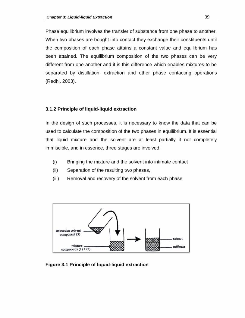
Chapter 3: Liquid-liquid Extraction 39
Phase equilibrium involves the transfer of substance from one phase to another.
When two phases are bought into contact they exchange their constituents until
the composition of each phase attains a constant value and equilibrium has
been attained. The equilibrium composition of the two phases can be very
different from one another and it is this difference which enables mixtures to be
separated by distillation, extraction and other phase contacting operations
(Redhi, 2003).
3.1.2 Principle of liquid-liquid extraction
In the design of such processes, it is necessary to know the data that can be
used to calculate the composition of the two phases in equilibrium. It is essential
that liquid mixture and the solvent are at least partially if not completely
immiscible, and in essence, three stages are involved:
(i) Bringing the mixture and the solvent into intimate contact
(ii) Separation of the resulting two phases,
(iii) Removal and recovery of the solvent from each phase
Figure 3.1 Principle of liquid-liquid extraction
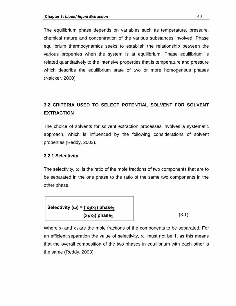
Chapter 3: Liquid-liquid Extraction 40
The equilibrium phase depends on variables such as temperature, pressure,
chemical nature and concentration of the various substances involved. Phase
equilibrium thermodynamics seeks to establish the relationship between the
various properties when the system is at equilibrium. Phase equilibrium is
related quantitatively to the intensive properties that is temperature and pressure
which describe the equilibrium state of two or more homogenous phases
(Naicker, 2000).
3.2 CRITERIA USED TO SELECT POTENTIAL SOLVENT FOR SOLVENT
EXTRACTION
The choice of solvents for solvent extraction processes involves a systematic
approach, which is influenced by the following considerations of solvent
properties (Reddy, 2003).
3.2.1 Selectivity
The selectivity, ω, is the ratio of the mole fractions of two components that are to
be separated in the one phase to the ratio of the same two components in the
other phase.
(3.1)
Where x2 and x3 are the mole fractions of the components to be separated. For
an efficient separation the value of selectivity, ω, must not be 1, as this means
that the overall composition of the two phases in equilibrium with each other is
the same (Reddy, 2003).
Selectivity (ω) = ( x2/x3) phase1
(x2/x3) phase2
Chapter 3: Liquid-liquid Extraction 41
3.2.2 The distribution coefficient
The capacity is described by distribution coefficient, K, which is the ratio of the
concentration of component to be separated in the solvent rich (extract) phase
to the ratio of the same component in the solvent depleted (raffinate) phase. K
should be large for a chosen solvent.
(3.2)
3.2.3 Ease of Recovery
Ideally a solvent which is easily separated from the mixture and then purified so
that it can be recycled and be re-used is desirable. For effective separation,
there should be a large difference in volatilities of the components in relation to
the solvent. There should be a high boiling point difference between the solvent
and the extracted components to ensure that the solvent can easily be
recovered by distillation.
3.2.4 Solvent Solubility
The solvent should have low solubility in one of the components, and separation
in the two phases region should be large. The latter presents a larger
composition range in which the solvent can be used.
A ternary phase diagram with the large two phase region implies a relatively
high mutual insolubility of the components in the ternary mixture. This is an
advantage as the useful composition range over which the extraction solvent
entrainer can be utilized is large as shown in figure 3.2 (Redhi, 2003).
K = (x2) phase1
(x2) phase2
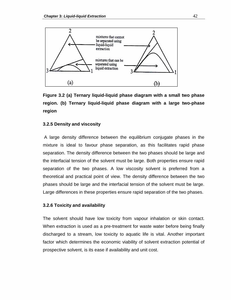
Chapter 3: Liquid-liquid Extraction 42
Figure 3.2 (a) Ternary liquid-liquid phase diagram with a small two phase
region. (b) Ternary liquid-liquid phase diagram with a large two-phase
region
3.2.5 Density and viscosity
A large density difference between the equilibrium conjugate phases in the
mixture is ideal to favour phase separation, as this facilitates rapid phase
separation. The density difference between the two phases should be large and
the interfacial tension of the solvent must be large. Both properties ensure rapid
separation of the two phases. A low viscosity solvent is preferred from a
theoretical and practical point of view. The density difference between the two
phases should be large and the interfacial tension of the solvent must be large.
Large differences in these properties ensure rapid separation of the two phases.
3.2.6 Toxicity and availability
The solvent should have low toxicity from vapour inhalation or skin contact.
When extraction is used as a pre-treatment for waste water before being finally
discharged to a stream, low toxicity to aquatic life is vital. Another important
factor which determines the economic viability of solvent extraction potential of
prospective solvent, is its ease if availability and unit cost.
Chapter 3: Liquid-liquid Extraction 43
3.3 THEORY AND REPRESENTATION OF TERNARY LIQUID-LIQUID
EQUILIBRIA
3.3.1 Introduction
The condition of phase equilibrium inherently involves the transfer of the solute
particles from one phase to another phase in a dynamic fashion. It is achieved
when the composition of the phase in contact with one another becomes
constant, that is, there is no net transfer of solute particles between the phases
3.3.2 Phase rule
In one of the most elegant calculations in the field of chemical thermodynamics
J.W. Gibbs deduced the phase rule. According to the Phase Rule (Barrow,
1996):
(3.3)
Where F is the variance of the system, which the number of intensive variables
that can changed, without changing the number of phases in equilibrium. C
refers to the number of the components in the system and P is the number of
phases (Atkins, 2002). For a three component system (this work):
(3.4)
Holding the temperature and pressure constant leaves two degrees freedom,
that is, the mole fractions of two of the components.
F= C-P+2
F= 5-P
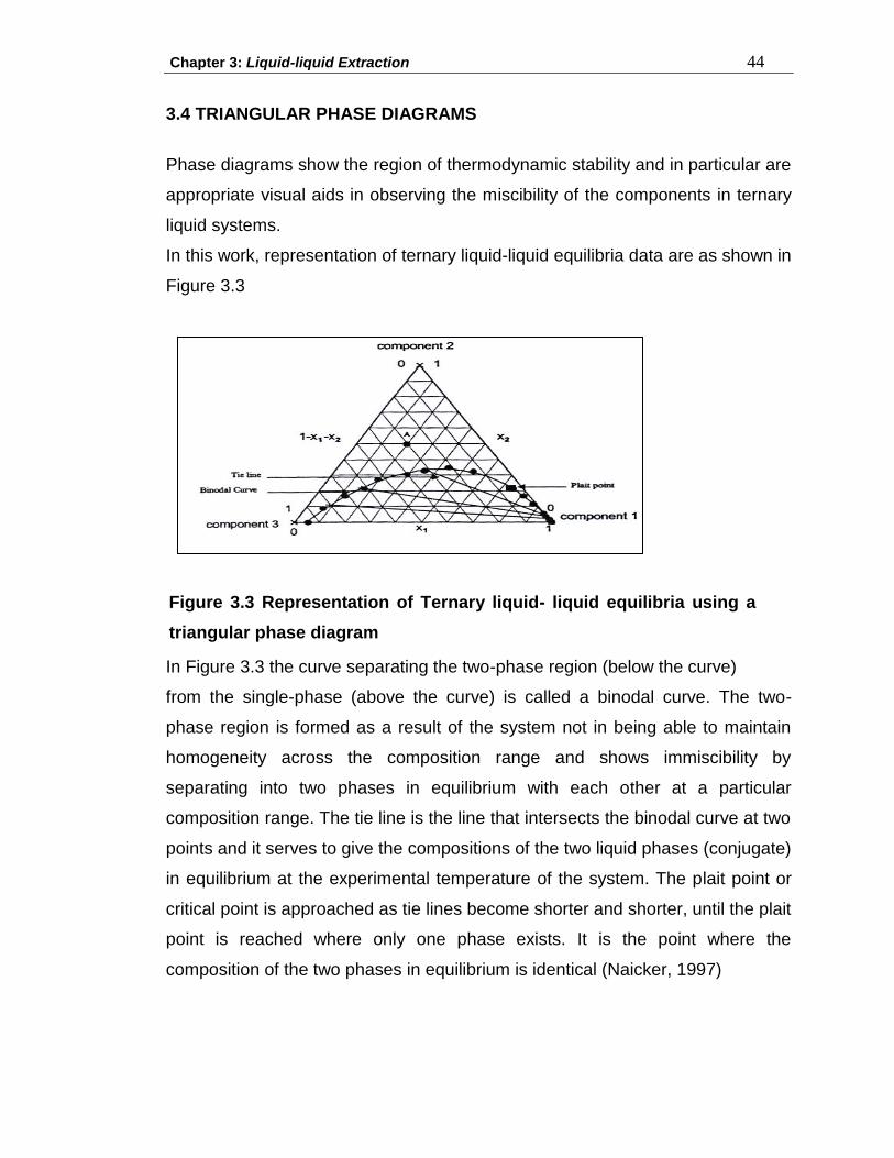
Chapter 3: Liquid-liquid Extraction 44
3.4 TRIANGULAR PHASE DIAGRAMS
Phase diagrams show the region of thermodynamic stability and in particular are
appropriate visual aids in observing the miscibility of the components in ternary
liquid systems.
In this work, representation of ternary liquid-liquid equilibria data are as shown in
Figure 3.3
In Figure 3.3 the curve separating the two-phase region (below the curve)
from the single-phase (above the curve) is called a binodal curve. The two-
phase region is formed as a result of the system not in being able to maintain
homogeneity across the composition range and shows immiscibility by
separating into two phases in equilibrium with each other at a particular
composition range. The tie line is the line that intersects the binodal curve at two
points and it serves to give the compositions of the two liquid phases (conjugate)
in equilibrium at the experimental temperature of the system. The plait point or
critical point is approached as tie lines become shorter and shorter, until the plait
point is reached where only one phase exists. It is the point where the
composition of the two phases in equilibrium is identical (Naicker, 1997)
Figure 3.3 Representation of Ternary liquid- liquid equilibria using a
triangular phase diagram
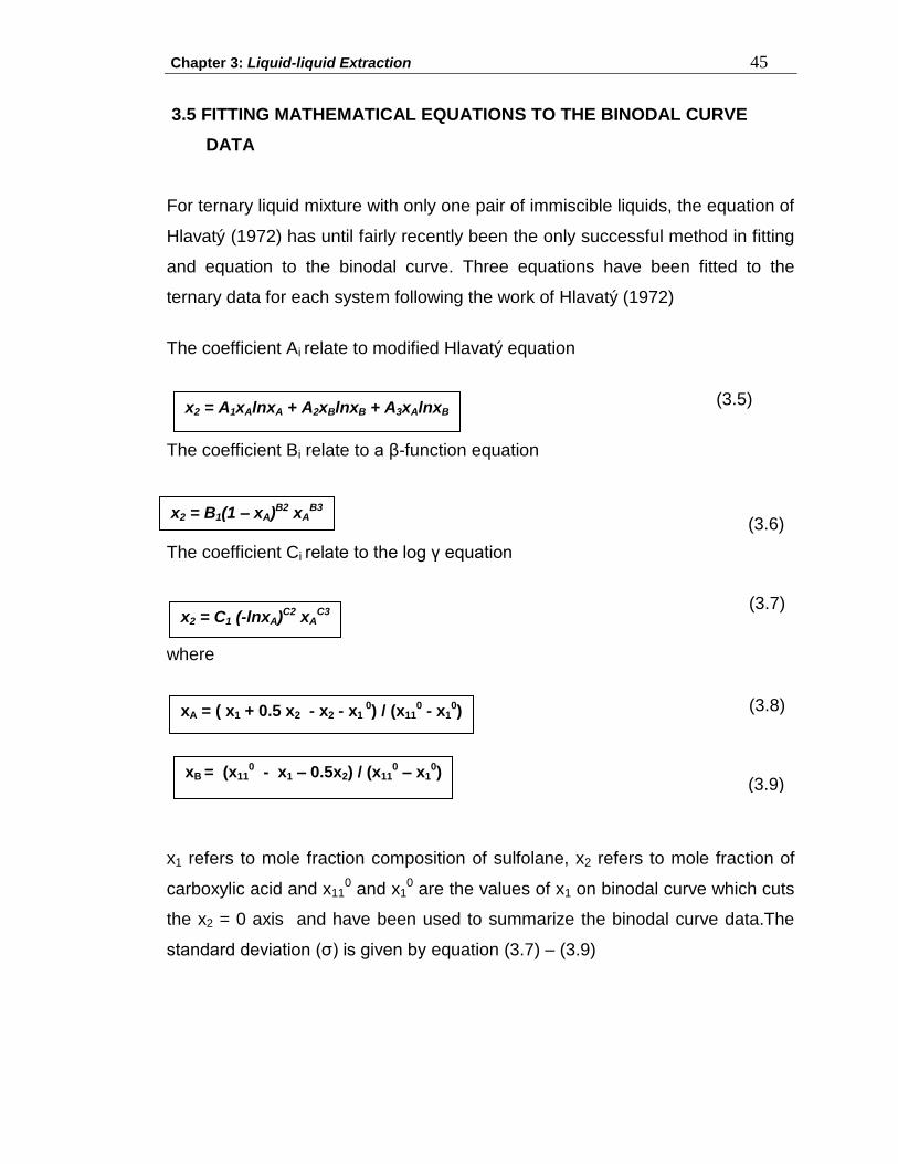
Chapter 3: Liquid-liquid Extraction 45
3.5 FITTING MATHEMATICAL EQUATIONS TO THE BINODAL CURVE
DATA
For ternary liquid mixture with only one pair of immiscible liquids, the equation of
Hlavatý (1972) has until fairly recently been the only successful method in fitting
and equation to the binodal curve. Three equations have been fitted to the
ternary data for each system following the work of Hlavatý (1972)
The coefficient Ai relate to modified Hlavatý equation
(3.5)
The coefficient Bi relate to a β-function equation
The coefficient Ci relate to the log γ equation
(3.7)
where
(3.8)
x1 refers to mole fraction composition of sulfolane, x2 refers to mole fraction of
carboxylic acid and x110 and x1
0 are the values of x1 on binodal curve which cuts
the x2 = 0 axis and have been used to summarize the binodal curve data.The
standard deviation (σ) is given by equation (3.7) – (3.9)
x2 = A1xAlnxA + A2xBlnxB + A3xAlnxB
x2 = B1(1 – xA)B2 xAB3
x2 = C1 (-lnxA)C2 xAC3
xA = ( x1 + 0.5 x2 - x2 - x1 0) / (x11
0 - x10)
xB = (x110 - x1 – 0.5x2) / (x11
0 – x10)
(3.6)
(3.9)
Chapter 3: Liquid-liquid Extraction 46
(3.10)
Where n is the number of data points and 3 is the number of estimated
coefficients (Sen and Srivastava, 1990).
3.6 CORRELATION OF TERNARY LIQUID-LIQUID EQUILIBRIA
3.6.1 Introduction
A significant fraction of chemical process design is concerned with separation of
fluid mixtures by diffusional operations. All design methods for such separations
require quantitative estimates of fluid-phase equilibria, and liquid phase activity
coefficients must be known.
Two models will be discussed, namely Non-Random, Two Liquid (NRTL)
equation, and Universal Quasi-Chemical (UNIQUAC) equation.
In the NTRL equation, the consideration is given to the prediction of ternary
vapour and ternary liquid-liquid equilibria based on the binary data and
UNIQUAC is applicable to multicomponent mixtures of non-polar and polar
liquids and encountered in typical chemical and petrochemicals systems (Redhi,
2003).
σ = ∑[x2 (calc) - x2 (exp)]2 / (n – 3 )1/2
Chapter 3: Liquid-liquid Extraction 47
3.6.2 The NRTL (Non Random, two liquid) equation
To take into account non- randomness mixing, it is assumed that the relation
between the local fraction x21 and x11 is given by a modification of the equation
(3.11)
to the following equation
where α12 is constant characteristic of the non-randomness of the mixture.
Interchanging subscripts 1 and 2, yield
The local mole fractions are related by:
x12 + x22 =1
x21 = x2exp(α12-g12/RT)
x11 x1exp(α12-g22/RT)
x21 = x2exp(α12-g21/RT)
x11 x1exp(α12-g11/RT)
x21 = x2exp(-g21/RT)
x11 x1exp(-g11/RT)
x21 + x11 =1
(3.12)
(3.13)
(3.14)
(3.15)
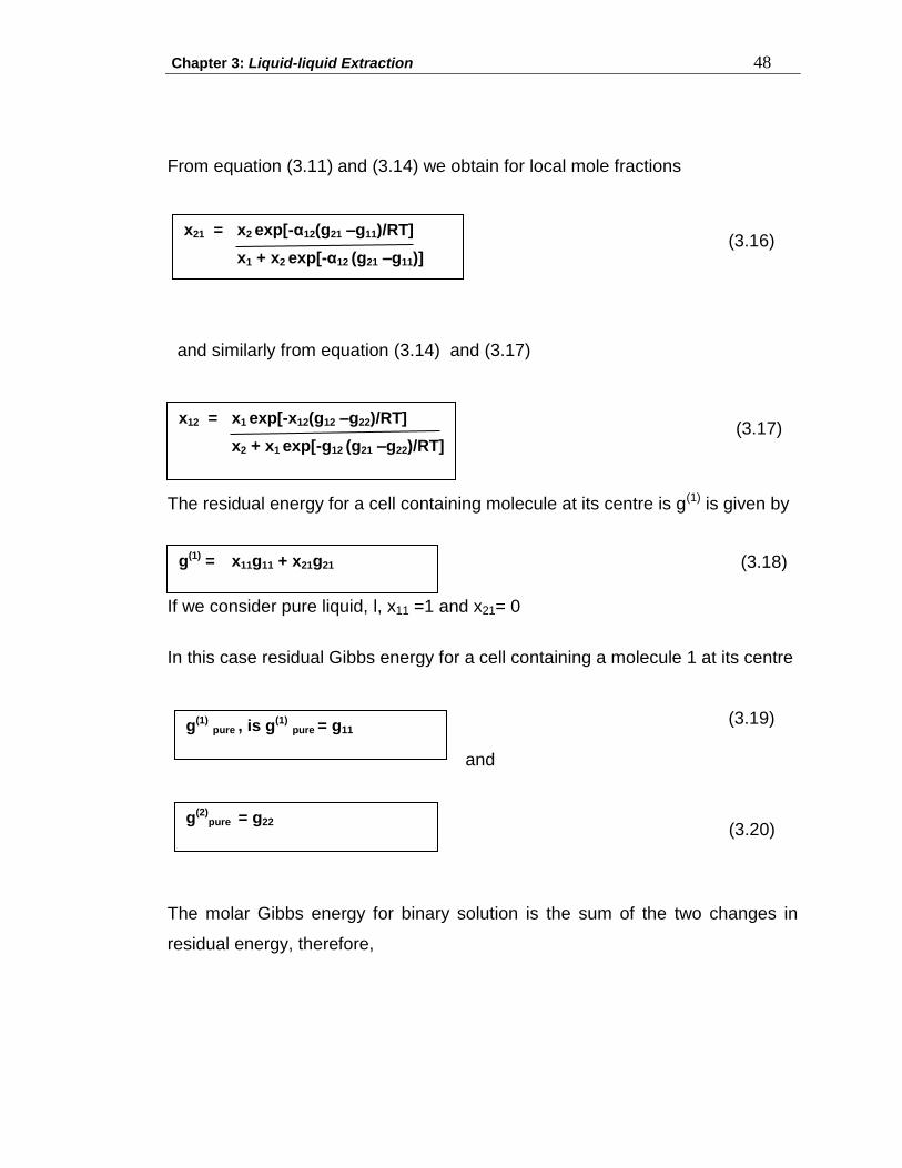
Chapter 3: Liquid-liquid Extraction 48
From equation (3.11) and (3.14) we obtain for local mole fractions
and similarly from equation (3.14) and (3.17)
The residual energy for a cell containing molecule at its centre is g(1) is given by
If we consider pure liquid, l, x11 =1 and x21= 0
In this case residual Gibbs energy for a cell containing a molecule 1 at its centre
and
The molar Gibbs energy for binary solution is the sum of the two changes in
residual energy, therefore,
x21 = x2 exp[-α12(g21 –g11)/RT]
x1 + x2 exp[-α12 (g21 –g11)]
x12 = x1 exp[-x12(g12 –g22)/RT]
x2 + x1 exp[-g12 (g21 –g22)/RT]
g(1) = x11g11 + x21g21
g(1) pure , is g(1) pure = g11
g(2)pure = g22
(3.16)
(3.17)
(3.18)
(3.19)
(3.20)
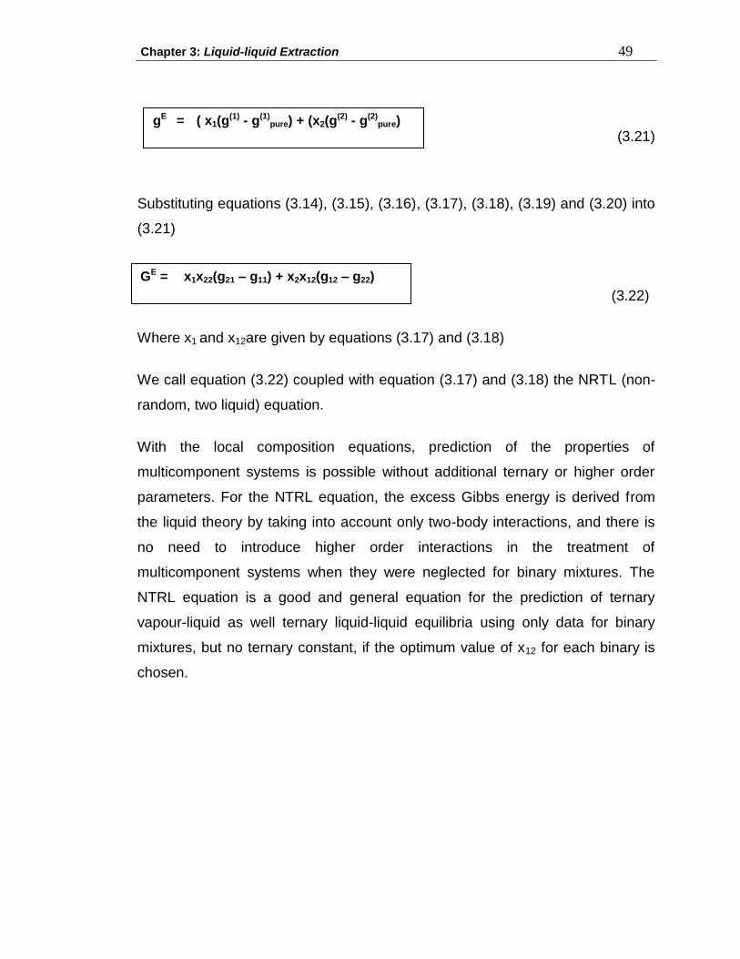
Chapter 3: Liquid-liquid Extraction 49
(3.21)
Substituting equations (3.14), (3.15), (3.16), (3.17), (3.18), (3.19) and (3.20) into
(3.21)
(3.22)
Where x1 and x12are given by equations (3.17) and (3.18)
We call equation (3.22) coupled with equation (3.17) and (3.18) the NRTL (non-
random, two liquid) equation.
With the local composition equations, prediction of the properties of
multicomponent systems is possible without additional ternary or higher order
parameters. For the NTRL equation, the excess Gibbs energy is derived from
the liquid theory by taking into account only two-body interactions, and there is
no need to introduce higher order interactions in the treatment of
multicomponent systems when they were neglected for binary mixtures. The
NTRL equation is a good and general equation for the prediction of ternary
vapour-liquid as well ternary liquid-liquid equilibria using only data for binary
mixtures, but no ternary constant, if the optimum value of x12 for each binary is
chosen.
gE = ( x1(g(1) - g(1)
pure) + (x2(g(2) - g(2)
pure)
GE = x1x22(g21 – g11) + x2x12(g12 – g22)
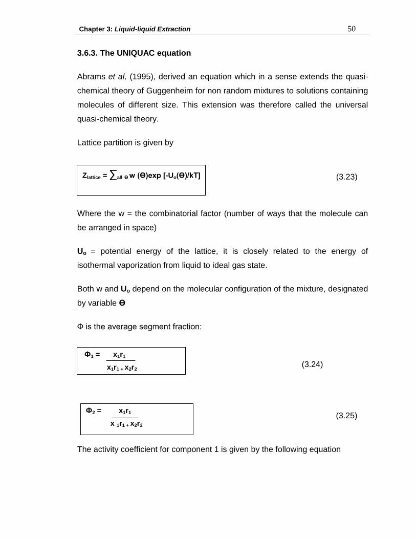
Chapter 3: Liquid-liquid Extraction 50
3.6.3. The UNIQUAC equation
Abrams et al, (1995), derived an equation which in a sense extends the quasi-
chemical theory of Guggenheim for non random mixtures to solutions containing
molecules of different size. This extension was therefore called the universal
quasi-chemical theory.
Lattice partition is given by
Where the w = the combinatorial factor (number of ways that the molecule can
be arranged in space)
Uo = potential energy of the lattice, it is closely related to the energy of
isothermal vaporization from liquid to ideal gas state.
Both w and Uo depend on the molecular configuration of the mixture, designated
by variable Ө
Ф is the average segment fraction:
(3.24)
The activity coefficient for component 1 is given by the following equation
Zlattice = ∑all Ө w (Ө)exp [-Uo(Ө)/kT]
Ф1 = x1r1
x1r1 + x2r2
Ф2 = x1r1
x 1r1 + x2r2
(3.23)
(3.25)
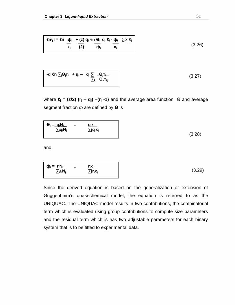
Chapter 3: Liquid-liquid Extraction 51
where ℓj = (z/2) (rj – qj) –(rj -1) and the average area function Ө and average
segment fraction ф are defined by Ө is
(3.28)
and
Since the derived equation is based on the generalization or extension of
Guggenheim‟s quasi-chemical model, the equation is referred to as the
UNIQUAC. The UNIQUAC model results in two contributions, the combinatorial
term which is evaluated using group contributions to compute size parameters
and the residual term which is has two adjustable parameters for each binary
system that is to be fitted to experimental data.
ℓnγi = ℓn фi + (z) qi ℓn Өi qi ℓi - фi ∑jxj ℓj
xi (2) фi xi
-qi ℓn ∑jӨjτji + qi – qi ∑j Өjτij
∑k Өkτkj
Өi = qiNi = qixi
∑iqiNj ∑jqixj
фi = riNi = rixi
∑iriNj ∑jrixj
(3.27)
(3.26)
(3.29)
Chapter 4: Experimental Techniques 52
CHAPTER 4
EXPERIMENTAL TECHNIQUES
4.1 Introduction
In principle the measurement of phase equilibria involves simply the
measurements of pressure, temperature, phase compositions and phase
amounts. In practise, however, it is not a simple matter to obtain experimental
data of sufficient accuracy, care must be taken to assure that equilibrium really
exists, that the temperature and pressure measured at the position where
equilibrium really exists, and that taking of samples for analysis does not disturb
the equilibrium appreciably (Redhi, 2003).
4.1.1 Phase diagram of mixtures
Phase diagram of a substance is a map that shows the conditions of
temperature and pressure at which its vapour or liquid phases are
thermodynamically most stable. Phase boundaries are the boundaries between
the regions and they show the values of temperature and pressure at which the
two neighbouring phases are equilibrium. Vapour pressure is a pressure of the
vapour in equilibrium with its condensed.
Phase diagram, of pure substances mixture show which phase is most stable for
a given condition. Composition is now a variable in addition to the pressure and
temperature (Barrow, 1998).
Chapter 4: Experimental Techniques 53
4.2 DETERMINATION OF THE BINODAL CURVES IN A TERNARY SYSTEM
4.2.1 Titration Method
Although the binodal curve does not yield complete information on phase
equilibria since it defines only the heterogeneous region, it can be used to
determine the composition of the conjugate phases when the properties of the
system studied are known (Redhi, 2003).
The titration method involves the addition of the third component to homogenous
binary mixtures of the components 1 and 2 until the appearance of the turbidity
or the attainment of the cloud-point (Reddy, 2003). The mixtures are well
agitated and kept at constant temperature. The determination of the tie line
compositions is to develop a standard curve that relates the composition of
points, through the concentration of one of the components of the binodal curve,
to an easily determined physical or chemical property such as density or
refractive index (Reddy, 2003, Naicker, 1997)
Two–phase mixtures across the entire mole fraction range were prepared and
allowed to reach equilibrium at constant temperature by allowing the mixtures to
mix and then separate completely from one another. The composition of the
conjugate phases were the analysed for the same physical property upon which
the standard curve was established. This measurement of physical property is
then correlated by means of the standard curve to obtain the compositions of the
conjugate phases and hence to establish the tie line.
This work the titration method, adapted from that Briggs and Comings (1943)
and modified by Letcher et al, (1989) was used. The binodal curve was first
determined by an analysis using refractive index, in order to determine the tie
line.
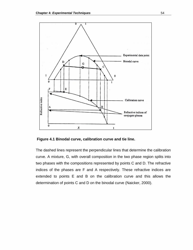
Chapter 4: Experimental Techniques 54
Figure 4.1 Binodal curve, calibration curve and tie line.
The dashed lines represent the perpendicular lines that determine the calibration
curve. A mixture, G, with overall composition in the two phase region splits into
two phases with the compositions represented by points C and D. The refractive
indices of the phases are F and A respectively. These refractive indices are
extended to points E and B on the calibration curve and this allows the
determination of points C and D on the binodal curve (Naicker, 2000).
Chapter 4: Experimental Techniques 55
4.3 DETERMINATION OF TIE-LINES IN A TERNARY SYSTEMS USING THE
BINODAL CURVE
4.3.1 Introduction
Measurement of refractive index or density of the mixture at equilibrium permits
the determination of corresponding position on the binodal curve, and thus tie-
line can be found.
4.3.2 Karl Fischer titration
As an alternative to refractive index method, tie lines could also be determined
using the Karl Fischer Method provides one of the components is water. In this
method the Karl Fischer reagent is used to titrate against the water in each
phase present. In this way the aqueous content of each can be determined, and
these compositions are located on the binodal curve and the tie lined are drawn.
4.4 DETERMINATION OF THE CRITICAL POINT (PLAIT POINT) IN THREE
COMPONENT SYSTEMS
The plait point or critical point is approached as tie lines become shorter and
shorter, until the plait point is reached where only one phase exists. It is the
point where the composition of the two phases in equilibrium is identical
(Naicker, 1997)
The plait point is determined by means of the Treybal method. The method of
Treybal involves producing plots of
x″1 vs x′1 (4.1) x″2 x′2
Chapter 4: Experimental Techniques 56
where x‟2, x‟3, x”
1, x”2 are the mole fraction compositions of the conjugate
mixtures and
x2 vs x2 x1 x1
where x1, x2 and x3 are the mole fraction compositions of components 1, 2 and 3,
respectively, of the mixture on the binodal curve. The plait point is that point of
intersection of the curves of (4.1) and (4.2).
4.5 REFRACTOMETRY
4.5.1 Introduction
The speed of light in a vacuum is always the same, but when light moves
through any other medium it travels more slowly since it is constantly being
absorbed and re-emitted by the atoms in the material.
The ratio of the speed of light in a vacuum to the speed of light in another
substance is defined as the index of refraction (refractive index or n) for the
substance,
Refractive Index of substance = (Speed of light in a vacuum) (Speed of light in a substance)
(4.2)
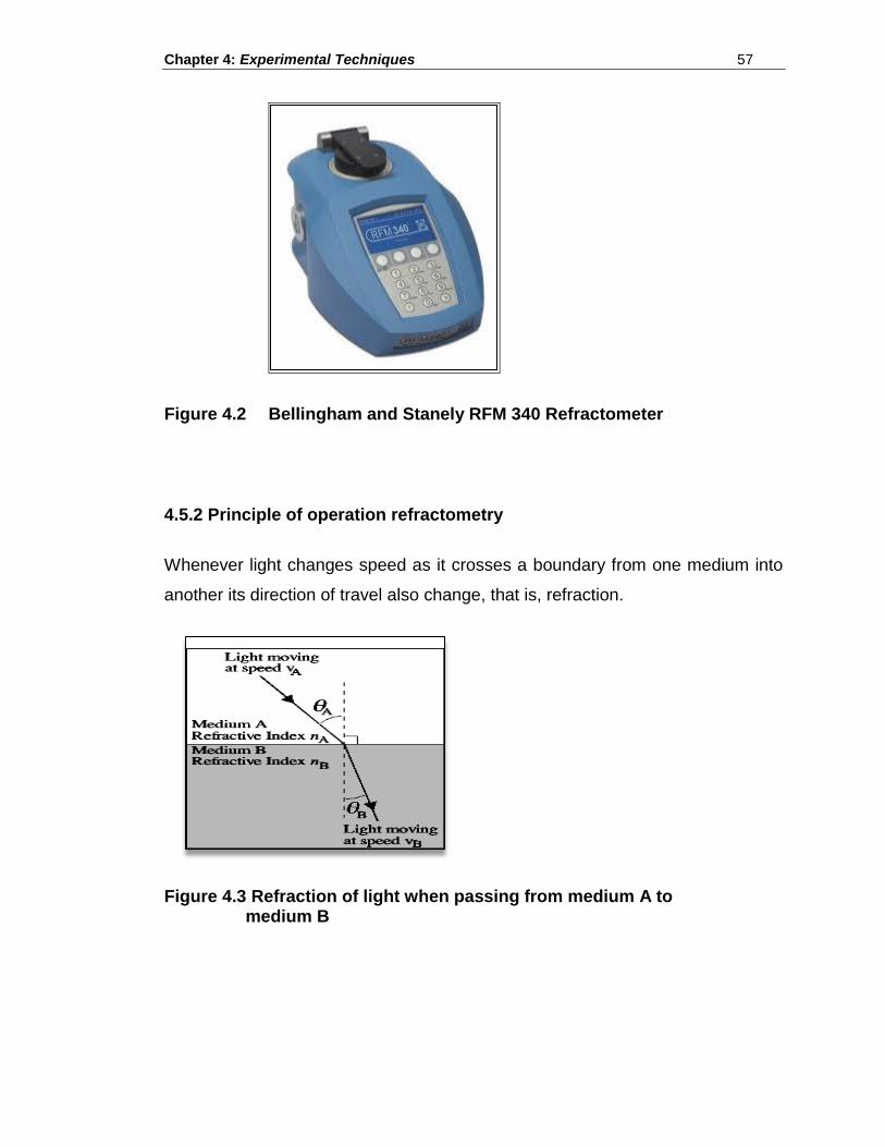
Chapter 4: Experimental Techniques 57
Figure 4.2 Bellingham and Stanely RFM 340 Refractometer
4.5.2 Principle of operation refractometry
Whenever light changes speed as it crosses a boundary from one medium into
another its direction of travel also change, that is, refraction.
Figure 4.3 Refraction of light when passing from medium A to medium B
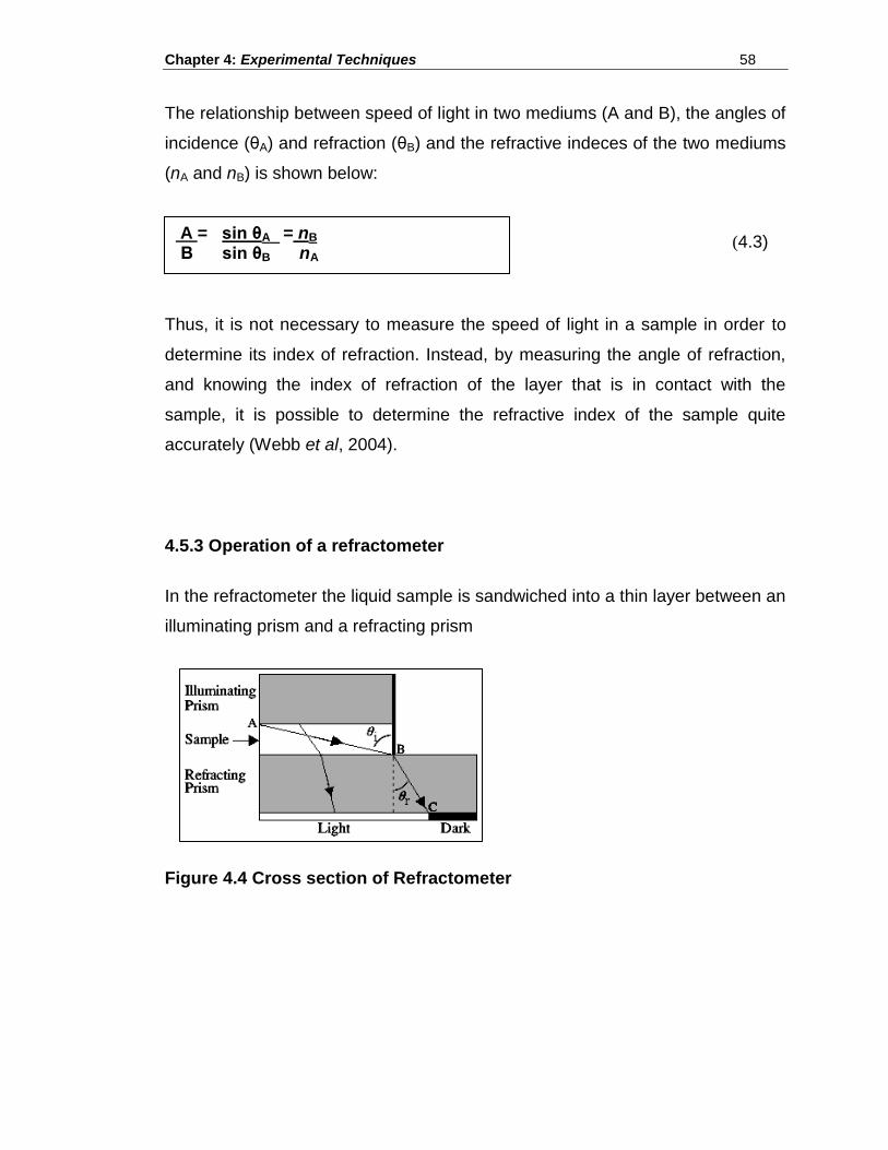
Chapter 4: Experimental Techniques 58
The relationship between speed of light in two mediums (A and B), the angles of
incidence (θA) and refraction (θB) and the refractive indeces of the two mediums
(nA and nB) is shown below:
Thus, it is not necessary to measure the speed of light in a sample in order to
determine its index of refraction. Instead, by measuring the angle of refraction,
and knowing the index of refraction of the layer that is in contact with the
sample, it is possible to determine the refractive index of the sample quite
accurately (Webb et al, 2004).
4.5.3 Operation of a refractometer
In the refractometer the liquid sample is sandwiched into a thin layer between an
illuminating prism and a refracting prism
Figure 4.4 Cross section of Refractometer
A = sin θA = nB
B sin θB nA
(4.3)
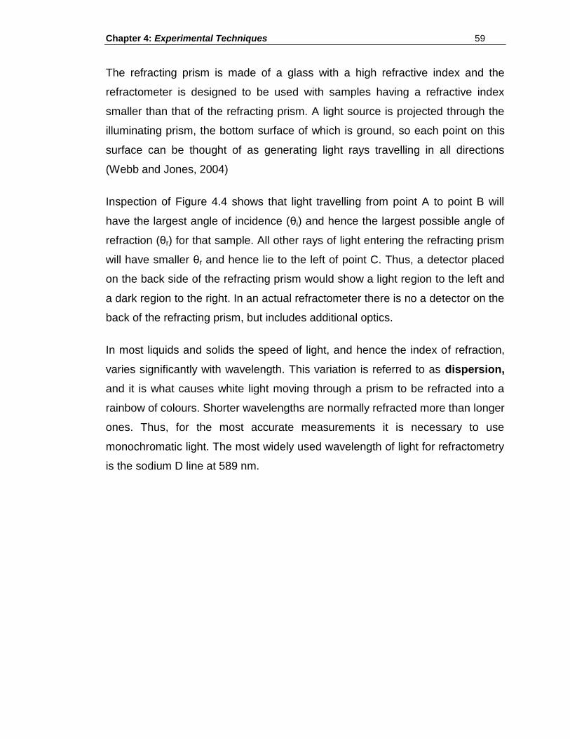
Chapter 4: Experimental Techniques 59
The refracting prism is made of a glass with a high refractive index and the
refractometer is designed to be used with samples having a refractive index
smaller than that of the refracting prism. A light source is projected through the
illuminating prism, the bottom surface of which is ground, so each point on this
surface can be thought of as generating light rays travelling in all directions
(Webb and Jones, 2004)
Inspection of Figure 4.4 shows that light travelling from point A to point B will
have the largest angle of incidence (θi) and hence the largest possible angle of
refraction (θr) for that sample. All other rays of light entering the refracting prism
will have smaller θr and hence lie to the left of point C. Thus, a detector placed
on the back side of the refracting prism would show a light region to the left and
a dark region to the right. In an actual refractometer there is no a detector on the
back of the refracting prism, but includes additional optics.
In most liquids and solids the speed of light, and hence the index of refraction,
varies significantly with wavelength. This variation is referred to as dispersion,
and it is what causes white light moving through a prism to be refracted into a
rainbow of colours. Shorter wavelengths are normally refracted more than longer
ones. Thus, for the most accurate measurements it is necessary to use
monochromatic light. The most widely used wavelength of light for refractometry
is the sodium D line at 589 nm.
Chapter 4: Experimental Techniques 60
4.6 EXCESS MOLAR VOLUMES
Excess molar data, like many data are more informative and easier to handle
when expressed relative to some of ideal behavior. The excess molar volume,
, is defined as:
(4.4)
where x1 is the mole fraction of component 1, Vmixture is the molar volume of
mixture and V ί o a molar of the component i. For binary mixture,
(4.5)
The change in the volume on mixing two liquids, especially two liquids, 1 and 2
can be attributed to a number of processes.
(a) the breakdown of 2-1 and 2-2 intermolecular interactions which have positive
effect on the volume,
(b) the formation of 1-2 intermolecular interactions which results in a dimunition
of the volume of the mixture,
(c) packing effects caused by difference in the size shape of the component
species and which may have positive or negative effect on the particular species
involved, and,
(d) formation of new chemical species
𝐕𝐦𝐄= Vmixture - ∑x1 V1
o
𝐕𝐦𝐄 = Vmixture – (x1 V1
o + x2 V2 o)
Chapter 4: Experimental Techniques 61
Volume changes on mixing of binary liquid mixtures, , at constant pressure
and temperature is of interest to chemists and chemical engineers, and is an
indicator of the non idealities present in real mixtures. There are great difficulties
in treating excess volumes and one major problem is the packing effect.
However, this has not deterred some theoreticians and a number of theories
abound.
4.6.1 Measurement of excess molar volumes
The excess molar volume, , is a helpful parameter in the design of the
technological processes of the reaction (Letcher and Reddy, 2002). The volume
changes of binary mixtures can be determined experimentally in one of two
ways, namely,
(i) indirectly from density measurements or
(ii) from the more direct dilatomeric method, that is by determining the resultant
volume change upon mixing of two components (Redhi, 2003).
Indirect determination
Density (p) is defined as:
(4.6)
where M is the mass of the substance, and V is the volume.
ρ = M V
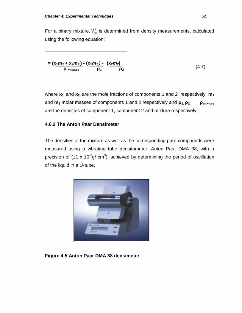
Chapter 4: Experimental Techniques 62
For a binary mixture, is determined from density measurements, calculated
using the following equation:
(4.7)
where x1 and x2 are the mole fractions of components 1 and 2 respectively, m1
and m2 molar masses of components 1 and 2 respectively and ρ1, ρ2, ρmixture
are the densities of component 1, component 2 and mixture respectively.
4.6.2 The Anton Paar Densimeter
The densities of the mixture as well as the corresponding pure compounds were
measured using a vibrating tube densitometer, Anton Paar DMA 38, with a
precision of (±1 x 10⁻⁵g/ cm3), achieved by determining the period of oscillation
of the liquid in a U-tube.
Figure 4.5 Anton Paar DMA 38 densimeter
= (x1m1 + x2m2 ) - (x1m1 ) + (x2m2) ρ mixture ρ1 ρ2
Chapter 4: Experimental Techniques 63
The natural vibration period of the tube, which depends on the density of the
liquid, is measured with a high-resolution digital frequency meter (Grguric et al,
2002).
(4.8)
Equation 4.8 is used to relate the density (ρ) and the period ( ) for the
investigated liquids ρ0 and 0, corresponding to the reference fluid. The value of
the constant A is determined by calibration using fluids of known densities. Air
and de-ionised water (Millipore quality) were used as reference fluids to
determine the constant of the densimeter.
The densimeter was calibrated each time measurements were done according
the procedure prescribed by the manufacturer. All measurements were in static
mode. The sample was introduced in a U-shaped sample tube, and the time
taken to equilibrate was typically between 5 to 7 minutes, after which the period
of oscillation was read from the numerical dial.
Between two successive measurements, the sample tube was cleaned with
acetone and dried for 5 minutes using the built in pump. This was the time
necessary for the period of empty sample tube to return to its previous value.
The density determination was based upon measurement of oscillations of
vibrating U-shape sample tube. The U-shaped tube was filled with liquid sample
mixture and the relationship between the between the period and the density
of the mixture ρ is given by:
(4.9)
Δρ = ρ - ρ0 = (A𝜏 2 – 𝜏02)
ρ = A + 𝐁𝝉2
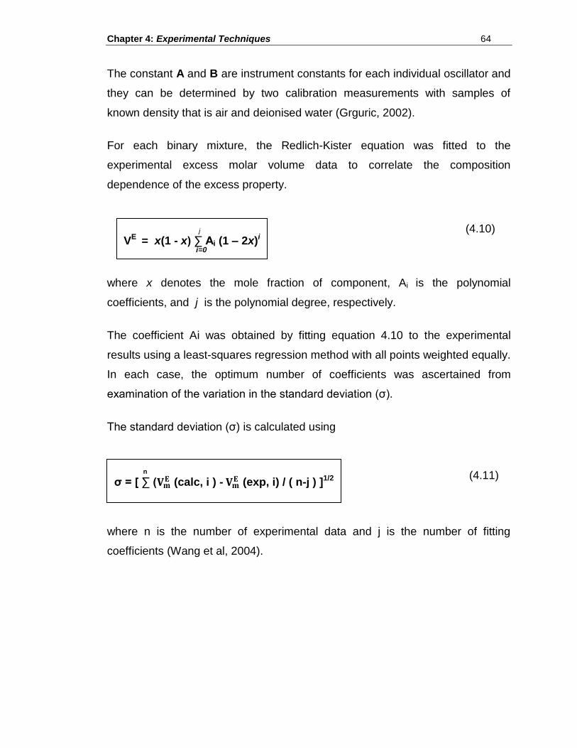
Chapter 4: Experimental Techniques 64
The constant A and B are instrument constants for each individual oscillator and
they can be determined by two calibration measurements with samples of
known density that is air and deionised water (Grguric, 2002).
For each binary mixture, the Redlich-Kister equation was fitted to the
experimental excess molar volume data to correlate the composition
dependence of the excess property.
where x denotes the mole fraction of component, Ai is the polynomial
coefficients, and j is the polynomial degree, respectively.
The coefficient Ai was obtained by fitting equation 4.10 to the experimental
results using a least-squares regression method with all points weighted equally.
In each case, the optimum number of coefficients was ascertained from
examination of the variation in the standard deviation (σ).
The standard deviation (σ) is calculated using
where n is the number of experimental data and j is the number of fitting
coefficients (Wang et al, 2004).
j
VE = x(1 - x) ∑ Ai (1 – 2x)i i=0
n
σ = [ ∑ (𝐕𝐦𝐄 (calc, i ) - 𝐕𝐦
𝐄 (exp, i) / ( n-j ) ]1/2
(4.10)
(4.11)
Chapter 4: Experimental Techniques 65
4.7 EXPERIMENTAL SECTION
4.7.1 Materials used
The solvents were kept in the dry box before use. Molecular sieves (4 nm) were
used to extract trace amount of moisture and the liquid were degassed in an
ultrasonic bath for one hour before use. The carboxylic acids and hydrocarbon
compounds were analysed by Karl-Fischer and showed that the water content
was less than 0.01 mass%. A summary of the materials used in this work, their
suppliers and purities is given in the table below.
Chapter 4: Experimental Techniques 66
Table 4.1 Materials used, their suppliers and mass % purities.
COMPOUND SUPPLIER % PURITY
Acetic acid Riedel-de Haën 99.8
Propanoic Acid Riedel-de Haën 99.8
Butanoic Acid Riedel-de Haën 99.8
2- Methylpropanoic acid Riedel-de Haën 99.8
Pentanoic acid Riedel-de Haën 99.8
3-Methylbutanoic acid Riedel-de Haën 99.8
Methanol Sigma -Aldrich 99.9
Ethanol Sigma -Aldrich 99.9
1-Propanol Sigma -Aldrich 99.9
2-Propanol Sigma -Aldrich 99.9
1-Butanol Sigma -Aldrich 99.9
2-Butanol Sigma -Aldrich 99.9
2-Methyl-1-propanol Sigma -Aldrich 99.9
2-Methyl-2-propanol Sigma -Aldrich 99.9
Sulfolane Fluka 99.5
Heptane Sigma -Aldrich 99.5
Dodecane Fluka 99.5
Cyclohexane Fluka 99.5
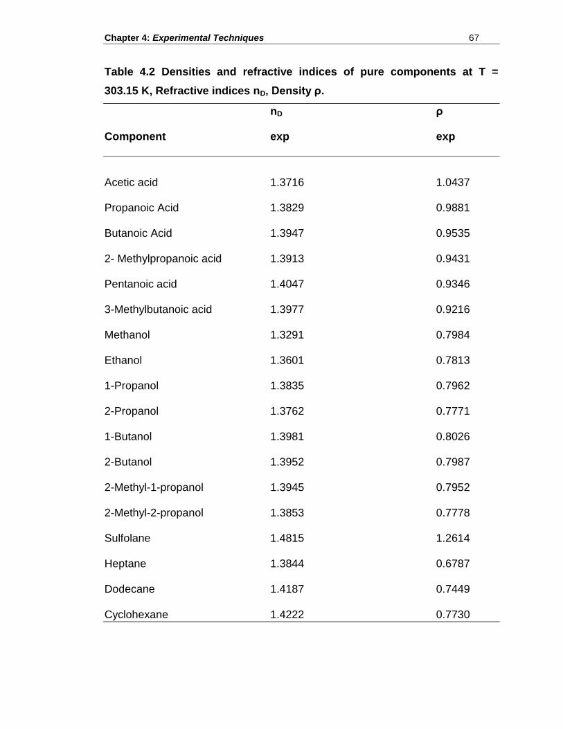
Chapter 4: Experimental Techniques 67
Table 4.2 Densities and refractive indices of pure components at T =
303.15 K, Refractive indices nD, Density ρ.
nD ρ Component exp exp
Acetic acid 1.3716 1.0437 Propanoic Acid 1.3829 0.9881 Butanoic Acid 1.3947 0.9535 2- Methylpropanoic acid 1.3913 0.9431 Pentanoic acid 1.4047 0.9346 3-Methylbutanoic acid 1.3977 0.9216 Methanol 1.3291 0.7984 Ethanol 1.3601 0.7813 1-Propanol 1.3835 0.7962 2-Propanol 1.3762 0.7771 1-Butanol 1.3981 0.8026 2-Butanol 1.3952 0.7987 2-Methyl-1-propanol 1.3945 0.7952 2-Methyl-2-propanol 1.3853 0.7778 Sulfolane 1.4815 1.2614 Heptane 1.3844 0.6787 Dodecane 1.4187 0.7449 Cyclohexane 1.4222 0.7730
Chapter 4: Experimental Techniques 68
4.7.2 Samples used for ternary system
4.7.2.1 System I
Carboxylic acids, that is, acetic acid (C2), propanoic acid (C3), butanoic acid
(C4), 2-methylpropanoic acid (C4), pentanoic acid (C5) and 3-methylbutanoic
acid (C5) as well as heptane and sulfolane were stored under 4nm molecular
sieves before use. Analysis of moisture content by Karl Fischer technique
showed that in all cases the water content was less than 0.01 mass %.
Sulfolane was supplied by Fluka and used without further purification. A
summary of the materials, their suppliers and purities, used in this work is given
in table 4.1. Mixtures of sulfolane and carboxylic acids were prepared in conical
flasks.
4.7.2.2 System II
Carboxylic acids, that is, acetic acid (C2), propanoic acid (C3), butanoic acid
(C4), 2-methylpropanoic acid (C4) pentanoic acid (C5) and 3-methylbutanoic acid
(C5) as well as cyclohexane and sulfolane were stored under 4nm molecular
sieves before use. Analysis of moisture content by Karl Fischer technique
showed that in all cases the water content was less than 0.01 mass %.
Sulfolane was supplied by Fluka and used without further purification. A
summary of the materials, their suppliers and purities, used in this work is given
in table 4.1. Mixtures of sulfolane and carboxylic acids were prepared in conical
flasks
Chapter 4: Experimental Techniques 69
4.7.2.3 System III
Carboxylic acids, that is, acetic acid (C2), propanoic acid (C3), butanoic acid
(C4), 2-methyl propanoic acid (C4) pentanoic acid (C5) and 3-methyl butanoic
acid (C5) as well as dodecane and sulfolane were stored under 4nm molecular
sieves before use. Analysis of moisture content by Karl Fischer technique
showed that in all cases the water content was less than 0.01 mass %.
Sulfolane was supplied by Fluka and used without further purification. A
summary of the materials, their suppliers and purities, used in this work is given
in table 4.1. Mixtures of sulfolane and carboxylic acids were prepared in conical
flasks.
4.7.2.4 System IV
Alcohols, that is, methanol (C1), ethanol (C2), 1-propanol (C3), 2-propanol (C3),
1-butanol (C4), 2-butanol (C4), 2-methyl-1-propanol (C4), 2-methyl-2-propanol
(C4), as well as heptane and sulfolane were stored under 4nm molecular sieves
before use. Analysis of moisture content by Karl Fischer technique showed that
in all cases the water content was less than 0.01 mass %. Sulfolane was
supplied by Fluka and used without further purification. A summary of the
materials, their suppliers and purities, used in this work is given in table 4.1.
Mixtures of sulfolane and alcohols were prepared in conical flasks.
4.7.3 Procedure
In this study, the “method of titration”, that is a method adapted from Briggs and
Comings (1943) as described by Letcher and Siswana (1992) was used to
determine the ternary liquid-liquid equilibrium data. Here the binodal curve was
first obtained and tie-lines were then determined.
Chapter 4: Experimental Techniques 70
The points on the curve were obtained in the following way, a mixture of two of
the miscible components, that is the carboxylic acid and sulfolane, were
prepared accurately by weighing. The mixtures were then left to equilibrate in a
water bath maintained at 30 ±0.1 0 C for at least 1 hour. The third component,
the hydrocarbon (heptane or cyclohexane or dodecane) was then added
dropwise from a weighed gas tight syringe until the mixture turned cloudy. The
syringe was weighed to determine the mass of hydrocarbon added.
To ensure the maintenance of one phase a measured drop of the carboxylic
acid was added in each case. At the hydrocarbon-rich end of the binodal curve
the binary mixture was made up of sulfolane and carboxylic acid (or alcohol),
and the third component added was the hydrocarbon. The mixtures of two of the
miscible components, the sulfolane and carboxylic acid (or alcohol), were
accurately prepared by weighing. The mixtures were then left to equilibrate in a
water bath at 30 ±0.10C for at least one hour.
The refractive index of the clear mixture was measured using a Bellingham &
Stanely RFM 340 Refractometer set at 30 ± 0.10C. A standard calibration curve
for each system was obtained by relating the refractive index of each mixture on
the co-existence curve, to a composition which was determined by dropping a
perpendicular from the co-existence curve to the sulfolane mole fraction axis.
The tie lines were determined from carefully made up solutions in the miscible
regions of the phase diagram.
The samples were then well shaken and left in a controlled water bath at 30 ±
0.10C for at least 24 hours to facilitate phase separation to ensure equilibrium.
Samples of the separate phases were then withdrawn using a warmed, gas tight
syringe and analysed immediately using the refractive index method. The
refractive indices of the different phases were then related to the compositions
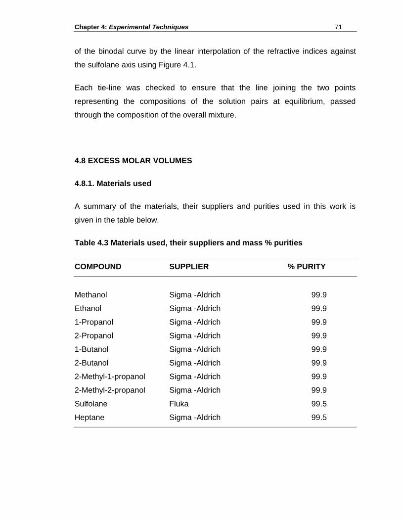
Chapter 4: Experimental Techniques 71
of the binodal curve by the linear interpolation of the refractive indices against
the sulfolane axis using Figure 4.1.
Each tie-line was checked to ensure that the line joining the two points
representing the compositions of the solution pairs at equilibrium, passed
through the composition of the overall mixture.
4.8 EXCESS MOLAR VOLUMES
4.8.1. Materials used
A summary of the materials, their suppliers and purities used in this work is
given in the table below.
Table 4.3 Materials used, their suppliers and mass % purities
COMPOUND SUPPLIER % PURITY
Methanol Sigma -Aldrich 99.9
Ethanol Sigma -Aldrich 99.9
1-Propanol Sigma -Aldrich 99.9
2-Propanol Sigma -Aldrich 99.9
1-Butanol Sigma -Aldrich 99.9
2-Butanol Sigma -Aldrich 99.9
2-Methyl-1-propanol Sigma -Aldrich 99.9
2-Methyl-2-propanol Sigma -Aldrich 99.9
Sulfolane Fluka 99.5
Heptane Sigma -Aldrich 99.5
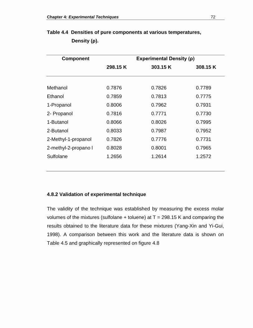
Chapter 4: Experimental Techniques 72
Table 4.4 Densities of pure components at various temperatures,
Density (ρ).
Component Experimental Density (ρ)
298.15 K 303.15 K 308.15 K
Methanol 0.7876 0.7826 0.7789
Ethanol 0.7859 0.7813 0.7775
1-Propanol 0.8006 0.7962 0.7931
2- Propanol 0.7816 0.7771 0.7730
1-Butanol 0.8066 0.8026 0.7995
2-Butanol 0.8033 0.7987 0.7952
2-Methyl-1-propanol 0.7826 0.7776 0.7731
2-methyl-2-propano l 0.8028 0.8001 0.7965
Sulfolane 1.2656 1.2614 1.2572
4.8.2 Validation of experimental technique
The validity of the technique was established by measuring the excess molar
volumes of the mixtures (sulfolane + toluene) at T = 298.15 K and comparing the
results obtained to the literature data for these mixtures (Yang-Xin and Yi-Gui,
1998). A comparison between this work and the literature data is shown on
Table 4.5 and graphically represented on figure 4.8
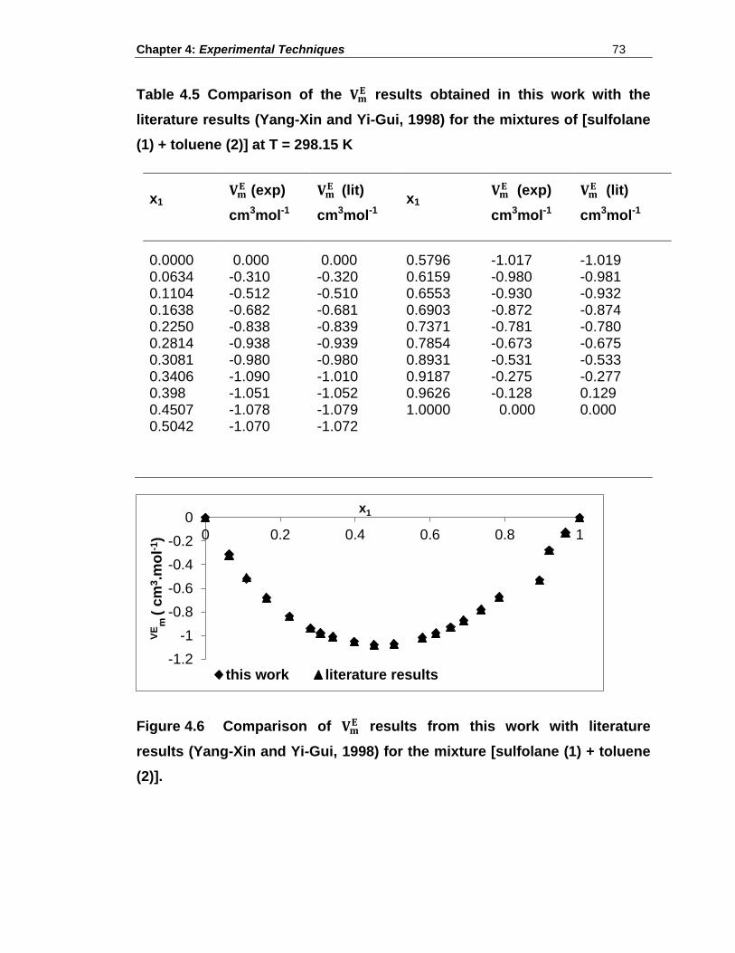
Chapter 4: Experimental Techniques 73
Table 4.5 Comparison of the results obtained in this work with the
literature results (Yang-Xin and Yi-Gui, 1998) for the mixtures of [sulfolane
(1) + toluene (2)] at T = 298.15 K
x1
(exp)
(lit) x1
(exp)
(lit)
cm3mol-1 cm3mol-1
cm3mol-1 cm3mol-1
0.0000 0.000 0.000 0.5796 -1.017 -1.019 0.0634 -0.310 -0.320 0.6159 -0.980 -0.981 0.1104 -0.512 -0.510 0.6553 -0.930 -0.932 0.1638 -0.682 -0.681 0.6903 -0.872 -0.874 0.2250 -0.838 -0.839 0.7371 -0.781 -0.780 0.2814 -0.938 -0.939 0.7854 -0.673 -0.675 0.3081 -0.980 -0.980 0.8931 -0.531 -0.533 0.3406 -1.090 -1.010 0.9187 -0.275 -0.277 0.398 -1.051 -1.052 0.9626 -0.128 0.129 0.4507 -1.078 -1.079 1.0000 0.000 0.000 0.5042 -1.070 -1.072
Figure 4.6 Comparison of results from this work with literature
results (Yang-Xin and Yi-Gui, 1998) for the mixture [sulfolane (1) + toluene
(2)].
-1.2
-1
-0.8
-0.6
-0.4
-0.2
0
0 0.2 0.4 0.6 0.8 1
VE
m ( c
m3.m
ol-
1)
x1
this work literature results
Chapter 4: Experimental Techniques 74
4.8.3 Preparation of samples mixtures
The pure solvents were initially degassed in an ultrasonic bath for at least 1
hour, as aerated solvents tend to give errors in density measurements as well as
tend to lead to non- reproducible readings. Moisture was removed by drying
pure solvent with molecular sieves (0.4nm). The mixtures were made up in glass
vial of 12 mL fitted with a lid. Mixtures with compositions spanning the entire
mole-fraction scale were made up gravimetrically. Care was taken to first add
the least volatile component into the vial and the complete mixture should have
left a small space, just large enough to aid the mixing in the vial. The mixtures
were made up just before use, and were shaken vigorously before injection.
4.8.4 Operation procedure for the instrument
Prior to each experimental run, the cell was first flushed with absolute ethanol
(>99.5%) and then acetone. After flushing, compressed air was blown through
the cell. The value of the constant periodic value, , for the sample tube filled
with air was then noted.
Double de-ionised Milli-Q water was then introduced into the cell by means of a
glass syringe with a Leur tip ensuring a snug and leak proof fit at the sample cell
syringe junction. The injection process was carried out slowly but steadily
enabling the liquid mixture to properly wet the walls of the cell, and also to
alleviate the risk of trapping air bubbles in the U-tube. The U-tube was first
flushed with 2 mL of the sample and the syringe then filled again with the
sample and introduced into the injection port.
Each measuring cycle was allowed to continue until a constant period value was
obtained. Period values for water, pure solvents and air were determined
between each solution injection, not only for density calculations, but as it also
permitted a continuous check on both sample purity and densitometer operation.
Chapter 4: Experimental Techniques 75
The density meter U tube cell was flushed with 10 % ethanol water solution after
each measurement to avoid the formation of air bubbles in the U tube. The
instrument was cleaned regularly with two vials of cleaning solution for the Anton
Paar Densimeter that was supplied by Swiss Lab, Instrument Supplier.
The densities of the mixture as well as the pure liquids were then determined
from the periodic values measured, and subsequent application of equation
(4.12)
Using the density and compositions of these mixtures was determined
according to equation
The temperature of the Anton Paar DMA 38 Densimeter was maintained at
303.15 + 0.002 K which was controlled by the internal solid-state thermostat.
𝐕𝐦𝐄 = Vmixture – (x1 V 1
o + x2 V2 o)
𝐕𝐦𝐄 = Vmixture - ∑x1 V1
o
(4.13)
Chapter 5: Results 76
CHAPTER 5
RESULTS
5. LIQUID–LIQUID EQUILIBRIA
The experimental liquid- liquid equilibria data are presented in the following
order:
Sulfolane (1) + Carboxylic Acid (2) + Heptane (3) at T = 303.15 K
Sulfolane (1) + Carboxylic Acid (2) + Cyclohexane (3) at T = 303.15 K
Sulfolane (1) + Carboxylic Acid (2) + Dodecane (3) at T = 303.15 K
Sulfolane (1) + Alcohol (2) + Heptane (3) at T = 303.15 K
For each section, tables of results for binodal curve data, calibration curve
data, tie-line data and coefficients of fitted equation, values of the parameters for
NTRL and UNIQUAC equations and selectivity data are tabulated. Ternary
phase diagrams, where UNIQUAC and NTRL thermodynamic models are used
to correlate the experimental data have been produced. Calibration curves as
well as distribution curves have also been included. The interaction parameters
for each model were determined with the aid of an LLE programme.
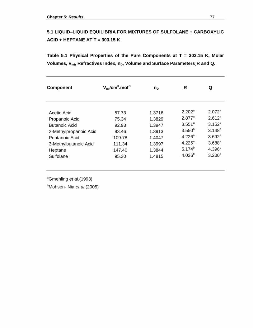
Chapter 5: Results 77
5.1 LIQUID–LIQUID EQUILIBRIA FOR MIXTURES OF SULFOLANE + CARBOXYLIC
ACID + HEPTANE AT T = 303.15 K
Table 5.1 Physical Properties of the Pure Components at T = 303.15 K, Molar
Volumes, Vmi, Refractives Index, nD, Volume and Surface Parameters, R and Q.
Component Vmi/cm3.mol-1 nD R Q
Acetic Acid 57.73 1.3716 2.202a 2.072a
Propanoic Acid 75.34 1.3829 2.877a 2.612a
Butanoic Acid 92.93 1.3947 3.551a 3.152a
2-Methylpropanoic Acid 93.46 1.3913 3.550a 3.148a
Pentanoic Acid 109.78 1.4047 4.226a 3.692a
3-Methylbutanoic Acid 111.34 1.3997 4.225a 3.688a
Heptane 147.40 1.3844 5.174b 4.396b
Sulfolane 95.30 1.4815 4.036b 3.200b
aGmehling et al.(1993)
bMohsen- Nia et al.(2005)
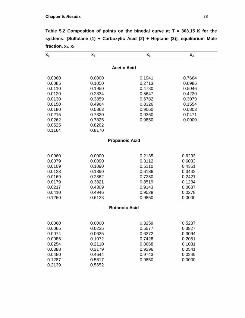
Chapter 5: Results 78
Table 5.2 Composition of points on the binodal curve at T = 303.15 K for the
systems: [Sulfolane (1) + Carboxylic Acid (2) + Heptane (3)], equilibrium Mole
fraction, x1, x2
x1 x2 x1 x2
Acetic Acid
0.0060
0.0000
0.1941
0.7664
0.0085
0.1050
0.2713
0.6986
0.0110
0.1950
0.4730
0.5046
0.0120
0.2834
0.5647
0.4220
0.0130
0.3859
0.6782
0.3079
0.0150
0.4964
0.8326
0.1554
0.0180
0.5863
0.9060
0.0803
0.0215
0.7320
0.9360
0.0471
0.0262
0.7825
0.9850
0.0000
0.0525
0.8202 0.1164
0.8170
Propanoic Acid
0.0060
0.0000
0.2135
0.6293
0.0079
0.0090
0.3112
0.6033
0.0109
0.1090
0.5110
0.4351
0.0123
0.1890
0.6186
0.3442
0.0169
0.2862
0.7280
0.2421
0.0179
0.3821
0.8519
0.1234
0.0217
0.4309
0.9143
0.0687
0.0410
0.4946
0.9528
0.0278
0.1260
0.6123
0.9850
0.0000
Butanoic Acid
0.0060
0.0000
0.3259
0.5237
0.0065
0.0235
0.5577
0.3827
0.0074
0.0635
0.6372
0.3094
0.0085
0.1072
0.7428
0.2051
0.0254
0.2110
0.8668
0.1031
0.0388
0.3179
0.9296
0.0541
0.0450
0.4644
0.9743
0.0249
0.1287
0.5617
0.9850
0.0000
0.2139
0.5652
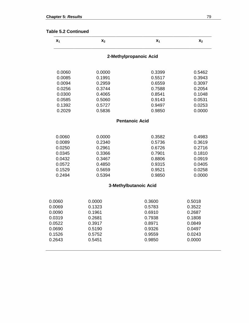
Chapter 5: Results 79
Table 5.2 Continued
x1
x2
x1
x2
2-Methylpropanoic Acid
0.0060
0.0000
0.3399
0.5462
0.0085
0.1991
0.5517
0.3943
0.0094
0.2959
0.6559
0.3097
0.0256
0.3744
0.7588
0.2054
0.0300
0.4065
0.8541
0.1048
0.0585
0.5060
0.9143
0.0531
0.1392
0.5727
0.9497
0.0253
0.2029
0.5836
0.9850
0.0000
Pentanoic Acid
0.0060
0.0000
0.3582
0.4983
0.0089
0.2340
0.5736
0.3619
0.0250
0.2961
0.6726
0.2716
0.0345
0.3366
0.7901
0.1810
0.0432
0.3467
0.8806
0.0919
0.0572
0.4850
0.9315
0.0405
0.1529
0.5659
0.9521
0.0258
0.2494
0.5394
0.9850
0.0000
3-Methylbutanoic Acid
0.0060
0.0000
0.3600
0.5018
0.0069
0.1323
0.5783
0.3522
0.0090
0.1961
0.6910
0.2687
0.0319
0.2681
0.7938
0.1808
0.0522
0.3917
0.8971
0.0849
0.0690
0.5190
0.9326
0.0497
0.1526
0.5752
0.9559
0.0243
0.2643
0.5451
0.9850
0.0000
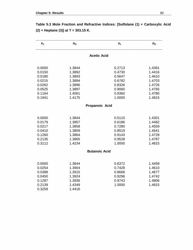
Chapter 5: Results 80
Table 5.3 Mole Fraction and Refractive Indices: [Sulfolane (1) + Carboxylic Acid
(2) + Heptane (3)] at T = 303.15 K.
x1
nD
x1
nD
Acetic Acid
0.0000
1.3844
0.2713
1.4391
0.0150
1.3892
0.4730
1.4416
0.0180
1.3893
0.5647
1.4610
0.0215
1.3894
0.6782
1.4703
0.0262
1.3896
0.8326
1.4726
0.0525
1.3897
0.9060
1.4765
0.1164
1.4061
0.9360
1.4780
0.1941
1.4175
1.0000
1.4815
Propanoic Acid
0.0000
1.3844
0.5110
1.4301
0.0179
1.3857
0.6186
1.4482
0.0217
1.3858
0.7280
1.4559
0.0410
1.3859
0.8519
1.4641
0.1260
1.3864
0.9143
1.4728
0.2135
1.3865
0.9528
1.4787
0.3112
1.4234
1.0000
1.4815
Butanoic Acid
0.0000
1.3844
0.6372
1.4458
0.0254
1.3904
0.7428
1.4610
0.0388
1.3915
0.8668
1.4677
0.0450
1.3924
0.9296
1.4742
0.1287
1.3936
0.9743
1.4806
0.2139
1.4349
1.0000
1.4815
0.3259
1.4416
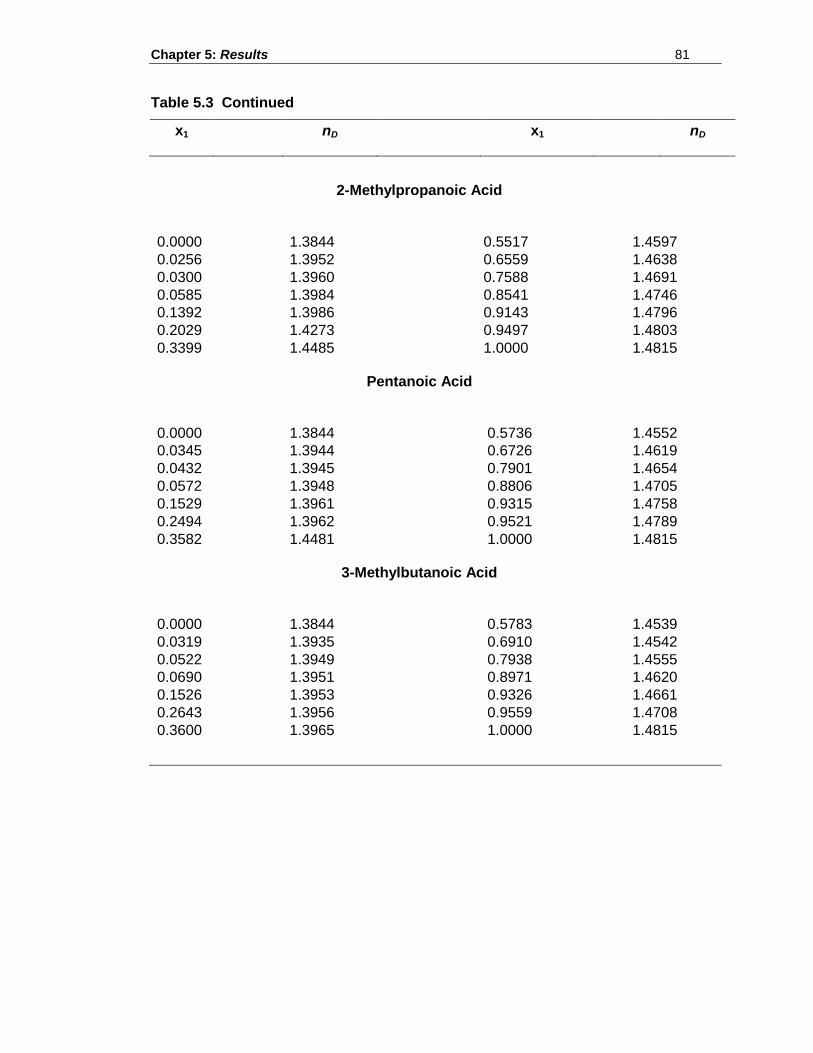
Chapter 5: Results 81
Table 5.3 Continued
x1
nD
x1
nD
2-Methylpropanoic Acid
0.0000
1.3844
0.5517
1.4597
0.0256
1.3952
0.6559
1.4638
0.0300
1.3960
0.7588
1.4691
0.0585
1.3984
0.8541
1.4746
0.1392
1.3986
0.9143
1.4796
0.2029
1.4273
0.9497
1.4803
0.3399
1.4485
1.0000
1.4815
Pentanoic Acid
0.0000
1.3844
0.5736
1.4552
0.0345
1.3944
0.6726
1.4619
0.0432
1.3945
0.7901
1.4654
0.0572
1.3948
0.8806
1.4705
0.1529
1.3961
0.9315
1.4758
0.2494
1.3962
0.9521
1.4789
0.3582
1.4481
1.0000
1.4815
3-Methylbutanoic Acid
0.0000
1.3844
0.5783
1.4539
0.0319
1.3935
0.6910
1.4542
0.0522
1.3949
0.7938
1.4555
0.0690
1.3951
0.8971
1.4620
0.1526
1.3953
0.9326
1.4661
0.2643
1.3956
0.9559
1.4708
0.3600
1.3965
1.0000
1.4815
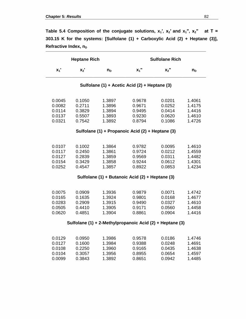
Chapter 5: Results 82
Table 5.4 Composition of the conjugate solutions, x1′, x2′ and x1″, x2″ at T =
303.15 K for the systems: [Sulfolane (1) + Carboxylic Acid (2) + Heptane (3)],
Refractive Index, nD
Heptane Rich Sulfolane Rich
x1' x2' nD x1" x2" nD
Sulfolane (1) + Acetic Acid (2) + Heptane (3)
0.0045 0.1050 1.3897 0.9678 0.0201 1.4061 0.0082 0.2711 1.3896 0.9671 0.0252 1.4175 0.0114 0.3829 1.3894 0.9495 0.0414 1.4416 0.0137 0.5507 1.3893 0.9230 0.0620 1.4610 0.0321 0.7542 1.3892 0.8794 0.1086 1.4726
Sulfolane (1) + Propanoic Acid (2) + Heptane (3)
0.0107 0.1002 1.3864 0.9782 0.0095 1.4610 0.0117 0.2450 1.3861 0.9724 0.0212 1.4559 0.0127 0.2839 1.3859 0.9569 0.0311 1.4482 0.0154 0.3429 1.3858 0.9244 0.0612 1.4301 0.0252 0.4547 1.3857 0.8922 0.0853 1.4234
Sulfolane (1) + Butanoic Acid (2) + Heptane (3)
0.0075 0.0909 1.3936 0.9879 0.0071 1.4742 0.0165 0.1635 1.3924 0.9801 0.0168 1.4677 0.0283 0.2909 1.3915 0.9490 0.0327 1.4610 0.0505 0.4410 1.3905 0.9171 0.0560 1.4458 0.0620 0.4851 1.3904 0.8861 0.0904 1.4416
Sulfolane (1) + 2-Methylpropanoic Acid (2) + Heptane (3)
0.0129 0.0950 1.3986 0.9578 0.0186 1.4746 0.0127 0.1600 1.3984 0.9388 0.0248 1.4691 0.0108 0.2250 1.3960 0.9165 0.0435 1.4638 0.0104 0.3057 1.3956 0.8955 0.0654 1.4597 0.0099 0.3843 1.3892 0.8651 0.0942 1.4485
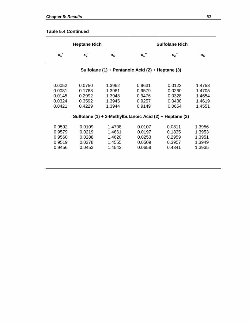
Chapter 5: Results 83
Table 5.4 Continued
Heptane Rich Sulfolane Rich
x1' x2' nD x1" x2" nD
Sulfolane (1) + Pentanoic Acid (2) + Heptane (3)
0.0052 0.0750 1.3962 0.9631 0.0123 1.4758 0.0081 0.1763 1.3961 0.9579 0.0260 1.4705 0.0145 0.2992 1.3948 0.9476 0.0328 1.4654 0.0324 0.3592 1.3945 0.9257 0.0438 1.4619 0.0421 0.4229 1.3944 0.9149 0.0654 1.4551
Sulfolane (1) + 3-Methylbutanoic Acid (2) + Heptane (3)
0.9592 0.0109 1.4708 0.0107 0.0811 1.3956 0.9579 0.0219 1.4661 0.0197 0.1835 1.3953 0.9560 0.0288 1.4620 0.0253 0.2959 1.3951 0.9519 0.0378 1.4555 0.0509 0.3957 1.3949 0.9456 0.0453 1.4542 0.0658 0.4841 1.3935
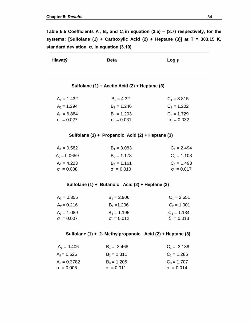
Chapter 5: Results 84
Table 5.5 Coefficients Ai, Bi, and Ci in equation (3.5) – (3.7) respectively, for the
systems: [Sulfolane (1) + Carboxylic Acid (2) + Heptane (3)] at T = 303.15 K,
standard deviation, σ, in equation (3.10)
Hlavatý
Beta
Log
Sulfolane (1) + Acetic Acid (2) + Heptane (3)
A1 = 1.432
B1 = 4.32
C1 = 3.815
A2 = 1.294
B2 = 1.246
C2 = 1.202
A3 = 6.884
B3 = 1.293
C3 = 1.729
σ = 0.027
σ = 0.031
σ = 0.032
Sulfolane (1) + Propanoic Acid (2) + Heptane (3)
A1 = 0.582
B1 = 3.083
C1 = 2.494
A2 = 0.0659
B2 = 1.173
C2 = 1.103
A3 = 4.223
B3 = 1.161
C3 = 1.493
σ = 0.008
σ = 0.010
σ = 0.017
Sulfolane (1) + Butanoic Acid (2) + Heptane (3)
A1 = 0.356
B1 = 2.906
C1 = 2.651
A2 = 0.216
B2 =1.206
C2 = 1.001
A3 = 1.089
B3 = 1.195
C3 = 1.134
σ = 0.007
σ = 0.012
Σ = 0.013
Sulfolane (1) + 2- Methylpropanoic Acid (2) + Heptane (3)
A1 = 0.406
B1 = 3.468
C1 = 3.188
A2 = 0.626
B2 = 1.311
C2 = 1.285
A3 = 0.3782
B3 = 1.205
C3 = 1.707
σ = 0.005
σ = 0.011
σ = 0.014
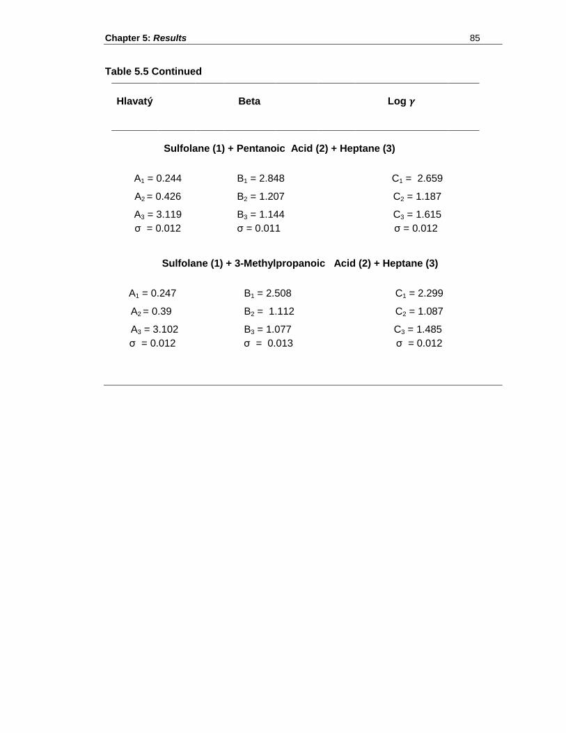
Chapter 5: Results 85
Table 5.5 Continued
Hlavatý
Beta
Log
Sulfolane (1) + Pentanoic Acid (2) + Heptane (3)
A1 = 0.244
B1 = 2.848
C1 = 2.659
A2 = 0.426
B2 = 1.207
C2 = 1.187
A3 = 3.119
B3 = 1.144
C3 = 1.615
σ = 0.012
σ = 0.011
σ = 0.012
Sulfolane (1) + 3-Methylpropanoic Acid (2) + Heptane (3)
A1 = 0.247
B1 = 2.508
C1 = 2.299
A2 = 0.39
B2 = 1.112
C2 = 1.087
A3 = 3.102
B3 = 1.077
C3 = 1.485
σ = 0.012
σ = 0.013
σ = 0.012
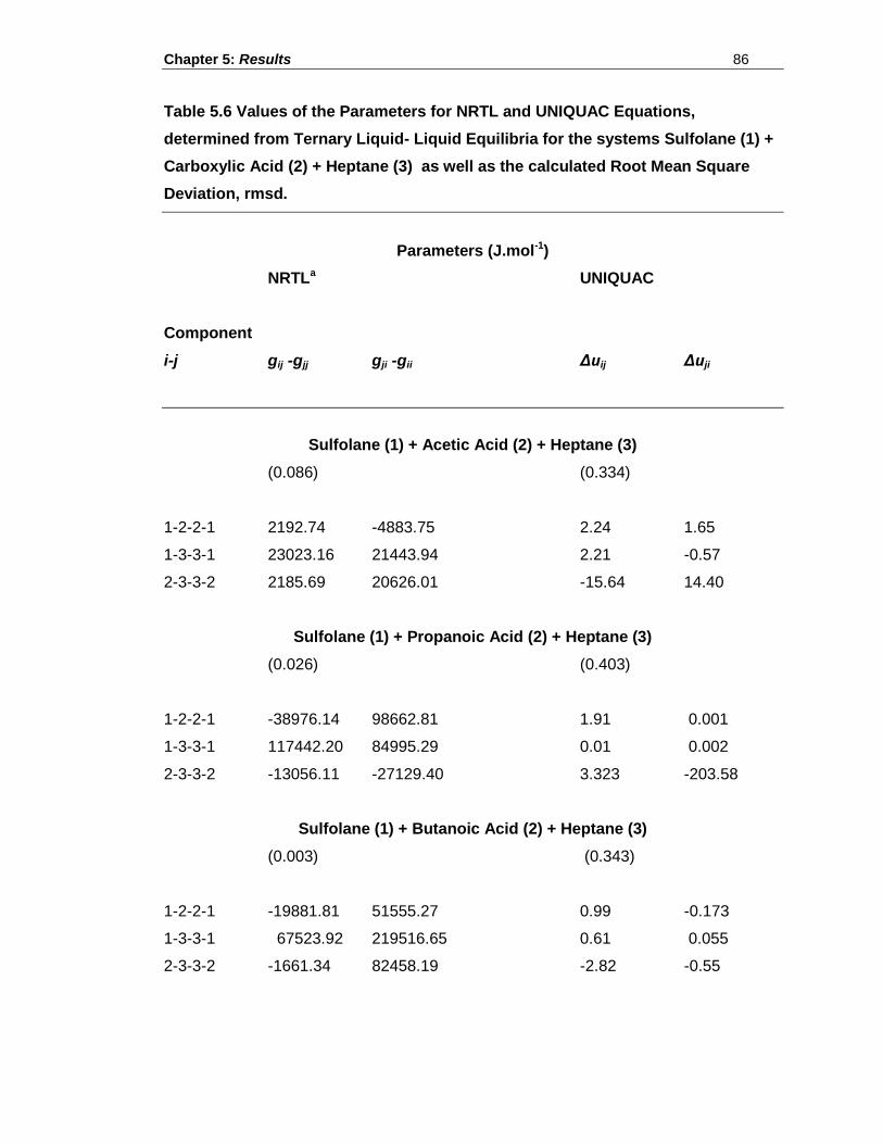
Chapter 5: Results 86
Table 5.6 Values of the Parameters for NRTL and UNIQUAC Equations,
determined from Ternary Liquid- Liquid Equilibria for the systems Sulfolane (1) +
Carboxylic Acid (2) + Heptane (3) as well as the calculated Root Mean Square
Deviation, rmsd.
Parameters (J.mol-1)
NRTLa UNIQUAC
Component
i-j gij -gjj gji -gii Δuij Δuji
Sulfolane (1) + Acetic Acid (2) + Heptane (3)
(0.086) (0.334)
1-2-2-1 2192.74 -4883.75 2.24 1.65
1-3-3-1 23023.16 21443.94 2.21 -0.57
2-3-3-2 2185.69 20626.01 -15.64 14.40
Sulfolane (1) + Propanoic Acid (2) + Heptane (3)
(0.026) (0.403)
1-2-2-1 -38976.14 98662.81 1.91 0.001
1-3-3-1 117442.20 84995.29 0.01 0.002
2-3-3-2 -13056.11 -27129.40 3.323 -203.58
Sulfolane (1) + Butanoic Acid (2) + Heptane (3)
(0.003) (0.343)
1-2-2-1 -19881.81 51555.27 0.99 -0.173
1-3-3-1 67523.92 219516.65 0.61 0.055
2-3-3-2 -1661.34 82458.19 -2.82 -0.55
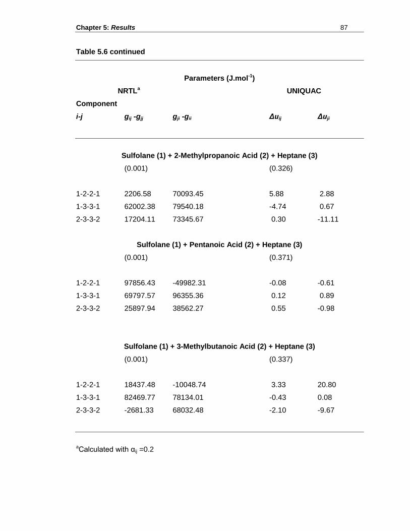
Chapter 5: Results 87
Table 5.6 continued
Parameters (J.mol-1)
NRTLa UNIQUAC
Component
i-j gij -gjj gji -gii Δuij Δuji
Sulfolane (1) + 2-Methylpropanoic Acid (2) + Heptane (3)
(0.001) (0.326)
1-2-2-1 2206.58 70093.45 5.88 2.88
1-3-3-1 62002.38 79540.18 -4.74 0.67
2-3-3-2 17204.11 73345.67 0.30 -11.11
Sulfolane (1) + Pentanoic Acid (2) + Heptane (3)
(0.001) (0.371)
1-2-2-1 97856.43 -49982.31 -0.08 -0.61
1-3-3-1 69797.57 96355.36 0.12 0.89
2-3-3-2 25897.94 38562.27 0.55 -0.98
Sulfolane (1) + 3-Methylbutanoic Acid (2) + Heptane (3)
(0.001) (0.337)
1-2-2-1 18437.48 -10048.74 3.33 20.80
1-3-3-1 82469.77 78134.01 -0.43 0.08
2-3-3-2 -2681.33 68032.48 -2.10 -9.67
aCalculated with αij =0.2
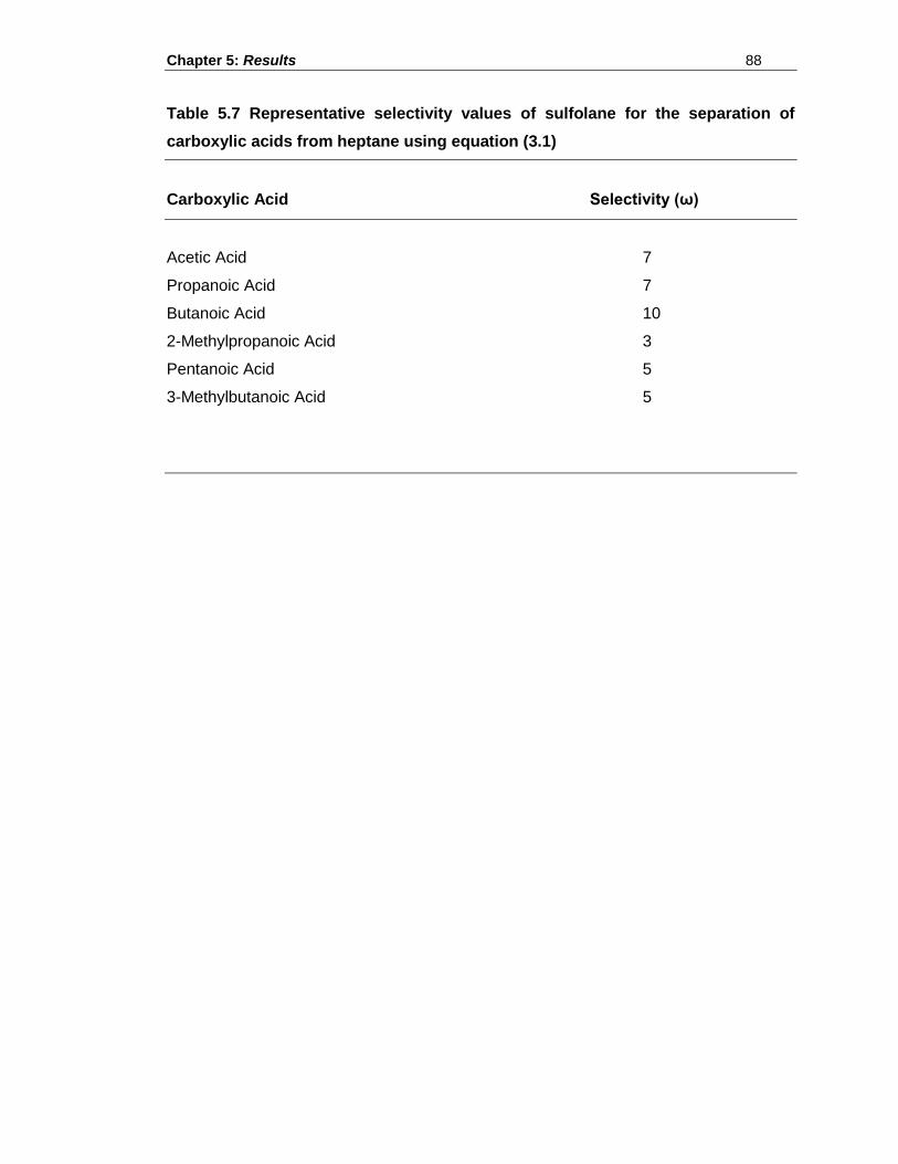
Chapter 5: Results 88
Table 5.7 Representative selectivity values of sulfolane for the separation of
carboxylic acids from heptane using equation (3.1)
Carboxylic Acid Selectivity (ω)
Acetic Acid 7
Propanoic Acid 7
Butanoic Acid 10
2-Methylpropanoic Acid 3
Pentanoic Acid 5
3-Methylbutanoic Acid 5
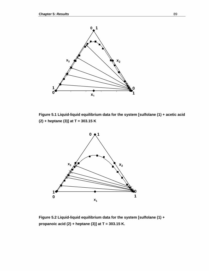
Chapter 5: Results 89
Figure 5.1 Liquid-liquid equilibrium data for the system [sulfolane (1) + acetic acid
(2) + heptane (3)] at T = 303.15 K
Figure 5.2 Liquid-liquid equilibrium data for the system [sulfolane (1) +
propanoic acid (2) + heptane (3)] at T = 303.15 K.
x2
x1
x3
1 0
0 1
0
1
x2 x3
x1
1 0
0 1
0 1
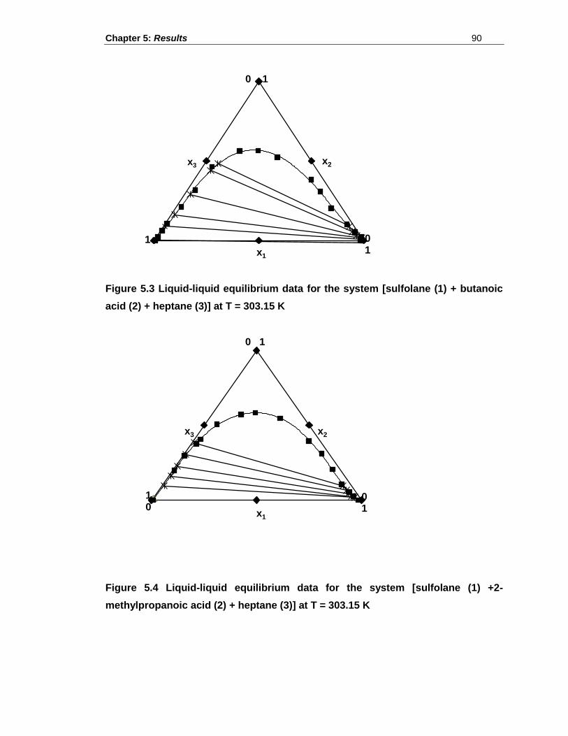
Chapter 5: Results 90
Figure 5.3 Liquid-liquid equilibrium data for the system [sulfolane (1) + butanoic
acid (2) + heptane (3)] at T = 303.15 K
Figure 5.4 Liquid-liquid equilibrium data for the system [sulfolane (1) +2-
methylpropanoic acid (2) + heptane (3)] at T = 303.15 K
x3 x2
x1
0 1
1 0 1
x2 x3
x1
0 1
1 0
0 1
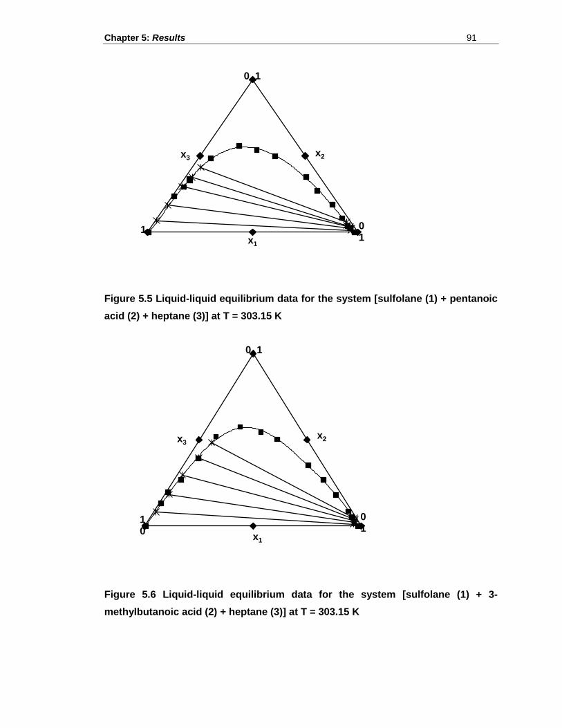
Chapter 5: Results 91
Figure 5.5 Liquid-liquid equilibrium data for the system [sulfolane (1) + pentanoic
acid (2) + heptane (3)] at T = 303.15 K
Figure 5.6 Liquid-liquid equilibrium data for the system [sulfolane (1) + 3-
methylbutanoic acid (2) + heptane (3)] at T = 303.15 K
x3 x2
x1
1 0 1
0 1
x3
x1
x2
0 1
0 1
1 0
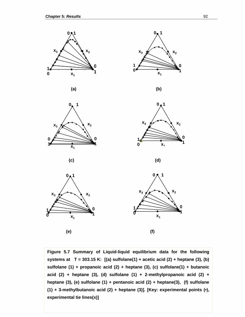
Chapter 5: Results 92
(a) (b)
(c) (d)
(e) (f)
x2
x1
x3
1 0
0 1
0
1
x2 x3
x1
1 0
0 1
0 1
x3 x2
x1
0 1
0 1
0 1
x2 x3
x1
0 1
1 0
0 1
x3 x2
x1
1 0
0 1
0 1
x3
x1
x2
0 1
0 1
1 0
Figure 5.7 Summary of Liquid-liquid equilibrium data for the following
systems at T = 303.15 K: [(a) sulfolane(1) + acetic acid (2) + heptane (3), (b)
sulfolane (1) + propanoic acid (2) + heptane (3), (c) sulfolane(1) + butanoic
acid (2) + heptane (3), (d) sulfolane (1) + 2-methylpropanoic acid (2) +
heptane (3), (e) sulfolane (1) + pentanoic acid (2) + heptane(3), (f) sulfolane
(1) + 3-methylbutanoic acid (2) + heptane (3)]. [Key: experimental points (▪),
experimental tie lines(x)]
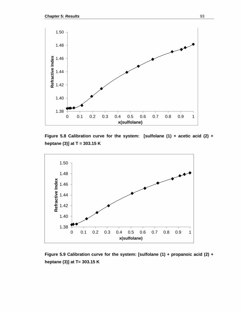
Chapter 5: Results 93
Figure 5.8 Calibration curve for the system: [sulfolane (1) + acetic acid (2) +
heptane (3)] at T = 303.15 K
Figure 5.9 Calibration curve for the system: [sulfolane (1) + propanoic acid (2) +
heptane (3)] at T= 303.15 K
1.38
1.40
1.42
1.44
1.46
1.48
1.50
0 0.1 0.2 0.3 0.4 0.5 0.6 0.7 0.8 0.9 1
Re
fra
cti
ve
In
de
x
x(sulfolane)
1.38
1.40
1.42
1.44
1.46
1.48
1.50
0 0.1 0.2 0.3 0.4 0.5 0.6 0.7 0.8 0.9 1
Refr
acti
ve In
dex
x(sulfolane)
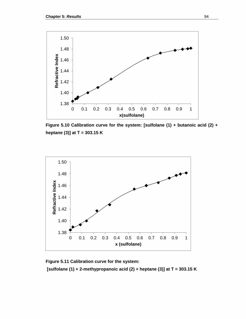
Chapter 5: Results 94
Figure 5.10 Calibration curve for the system: [sulfolane (1) + butanoic acid (2) +
heptane (3)] at T = 303.15 K
Figure 5.11 Calibration curve for the system:
[sulfolane (1) + 2-methypropanoic acid (2) + heptane (3)] at T = 303.15 K
1.38
1.40
1.42
1.44
1.46
1.48
1.50
0 0.1 0.2 0.3 0.4 0.5 0.6 0.7 0.8 0.9 1
Re
fra
cti
ve
In
de
x
x (sulfolane)
1.38
1.40
1.42
1.44
1.46
1.48
1.50
0 0.1 0.2 0.3 0.4 0.5 0.6 0.7 0.8 0.9 1
Re
fra
cti
ve
In
de
x
x(sulfolane)
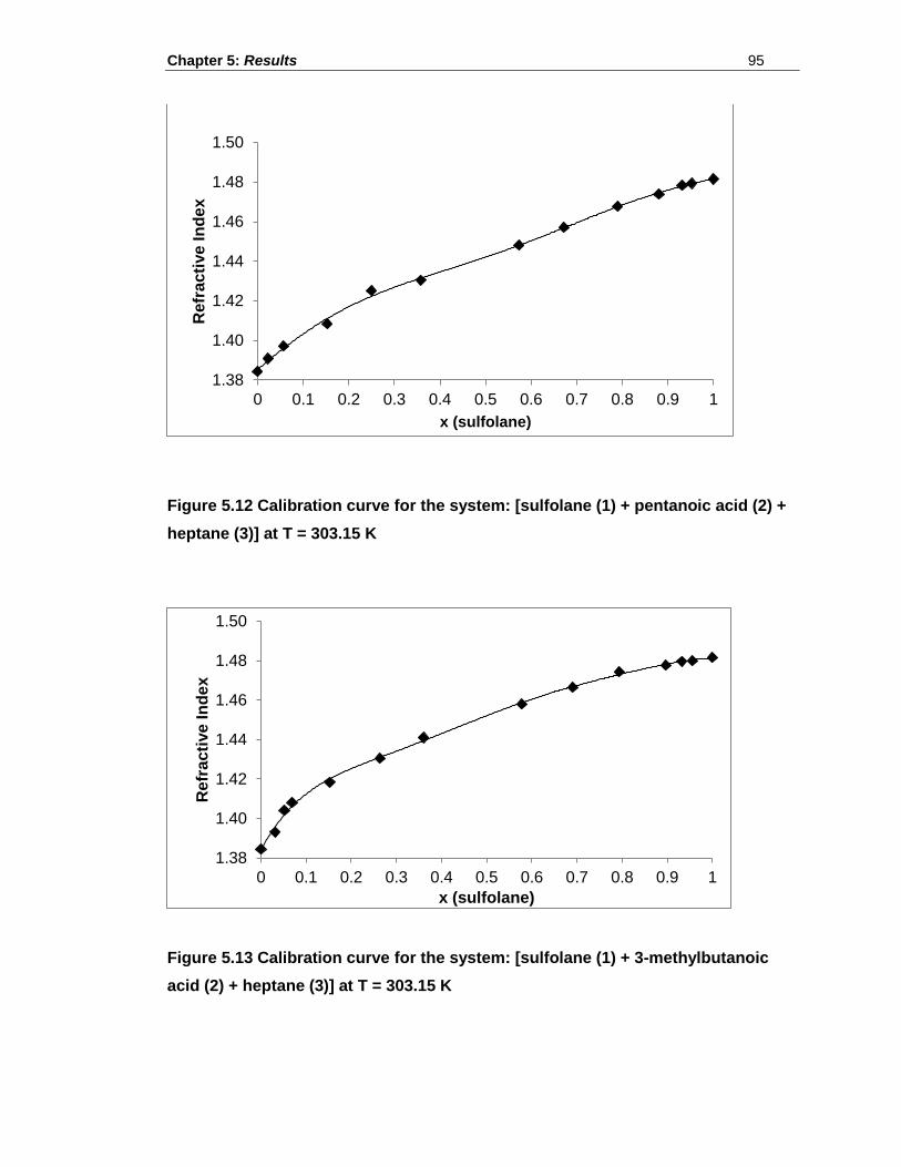
Chapter 5: Results 95
Figure 5.12 Calibration curve for the system: [sulfolane (1) + pentanoic acid (2) +
heptane (3)] at T = 303.15 K
Figure 5.13 Calibration curve for the system: [sulfolane (1) + 3-methylbutanoic
acid (2) + heptane (3)] at T = 303.15 K
1.38
1.40
1.42
1.44
1.46
1.48
1.50
0 0.1 0.2 0.3 0.4 0.5 0.6 0.7 0.8 0.9 1
Re
fra
cti
ve
In
de
x
x (sulfolane)
1.38
1.40
1.42
1.44
1.46
1.48
1.50
0 0.1 0.2 0.3 0.4 0.5 0.6 0.7 0.8 0.9 1
Re
fra
cti
ve
In
de
x
x (sulfolane)
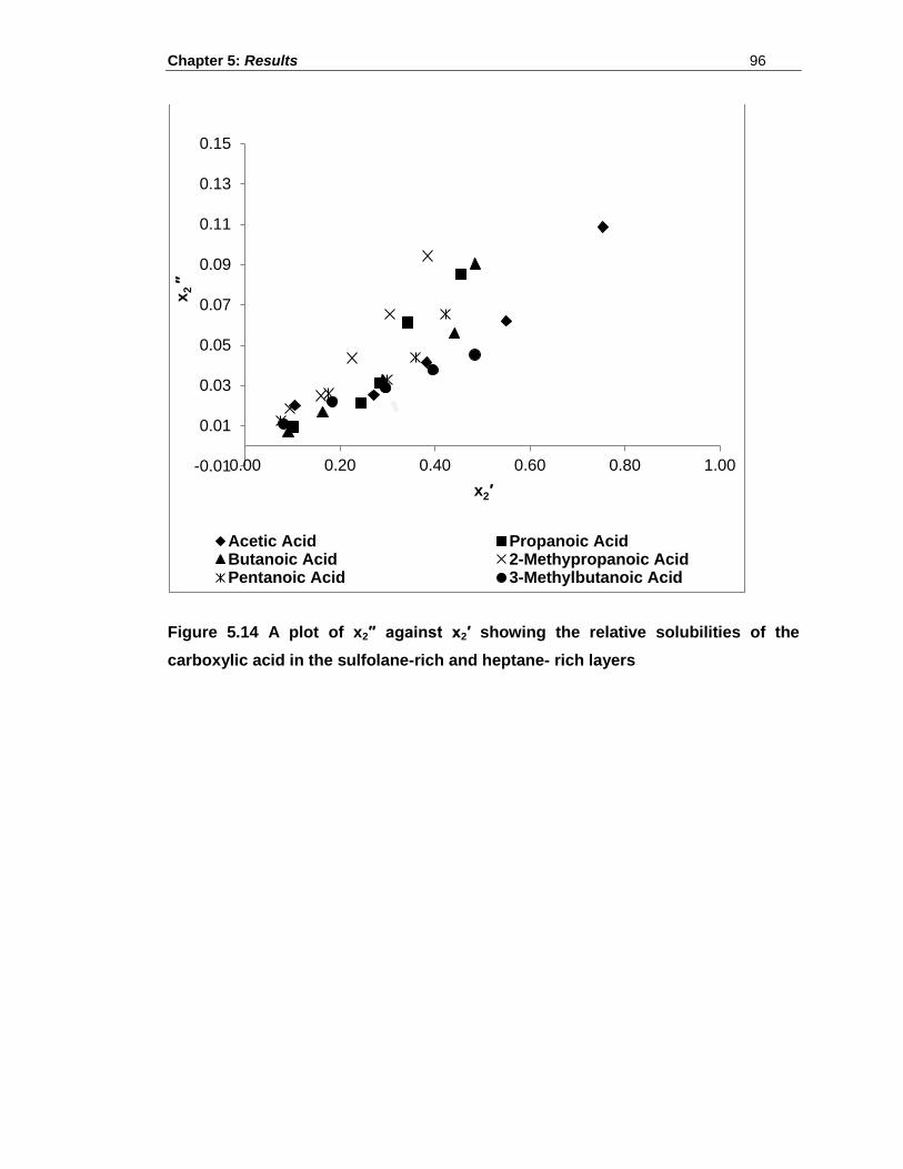
Chapter 5: Results 96
Figure 5.14 A plot of x2″ against x2′ showing the relative solubilities of the
carboxylic acid in the sulfolane-rich and heptane- rich layers
-0.01
0.01
0.03
0.05
0.07
0.09
0.11
0.13
0.15
0.00 0.20 0.40 0.60 0.80 1.00
x2
″
Acetic Acid Propanoic AcidButanoic Acid 2-Methypropanoic AcidPentanoic Acid 3-Methylbutanoic Acid
x2′
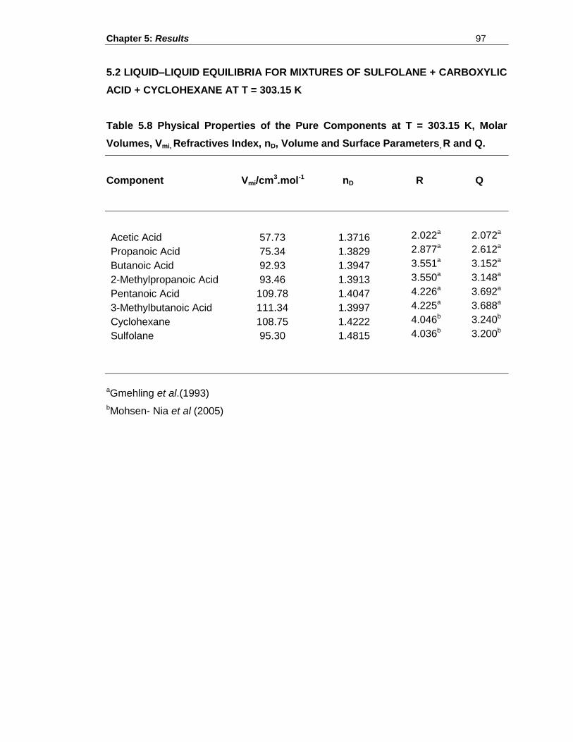
Chapter 5: Results 97
5.2 LIQUID–LIQUID EQUILIBRIA FOR MIXTURES OF SULFOLANE + CARBOXYLIC
ACID + CYCLOHEXANE AT T = 303.15 K
Table 5.8 Physical Properties of the Pure Components at T = 303.15 K, Molar
Volumes, Vmi, Refractives Index, nD, Volume and Surface Parameters, R and Q.
Component Vmi/cm3.mol-1 nD R Q
Acetic Acid 57.73 1.3716 2.022a 2.072a
Propanoic Acid 75.34 1.3829 2.877a 2.612a
Butanoic Acid 92.93 1.3947 3.551a 3.152a
2-Methylpropanoic Acid 93.46 1.3913 3.550a 3.148a
Pentanoic Acid 109.78 1.4047 4.226a 3.692a
3-Methylbutanoic Acid 111.34 1.3997 4.225a 3.688a
Cyclohexane 108.75 1.4222 4.046b 3.240b
Sulfolane 95.30 1.4815 4.036b 3.200b
aGmehling et al.(1993)
bMohsen- Nia et al (2005)
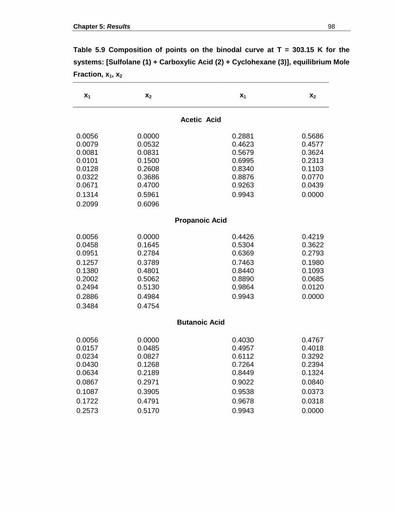
Chapter 5: Results 98
Table 5.9 Composition of points on the binodal curve at T = 303.15 K for the
systems: [Sulfolane (1) + Carboxylic Acid (2) + Cyclohexane (3)], equilibrium Mole
Fraction, x1, x2
x1
x2
x1
x2
Acetic Acid
0.0056
0.0000
0.2881
0.5686
0.0079
0.0532
0.4623
0.4577 0.0081
0.0831
0.5679
0.3624
0.0101
0.1500
0.6995
0.2313 0.0128
0.2608
0.8340
0.1103
0.0322
0.3686
0.8876
0.0770 0.0671
0.4700
0.9263
0.0439
0.1314
0.5961
0.9943
0.0000
0.2099
0.6096
Propanoic Acid 0.0056
0.0000
0.4426
0.4219
0.0458
0.1645
0.5304
0.3622 0.0951
0.2784
0.6369
0.2793
0.1257
0.3789
0.7463
0.1980 0.1380
0.4801
0.8440
0.1093
0.2002
0.5062
0.8890
0.0685 0.2494
0.5130
0.9864
0.0120
0.2886
0.4984
0.9943
0.0000
0.3484
0.4754
Butanoic Acid
0.0056
0.0000
0.4030
0.4767 0.0157
0.0485
0.4957
0.4018
0.0234
0.0827
0.6112
0.3292 0.0430
0.1268
0.7264
0.2394
0.0634
0.2189
0.8449
0.1324
0.0867
0.2971
0.9022
0.0840
0.1087
0.3905
0.9538
0.0373
0.1722
0.4791
0.9678
0.0318
0.2573
0.5170
0.9943
0.0000
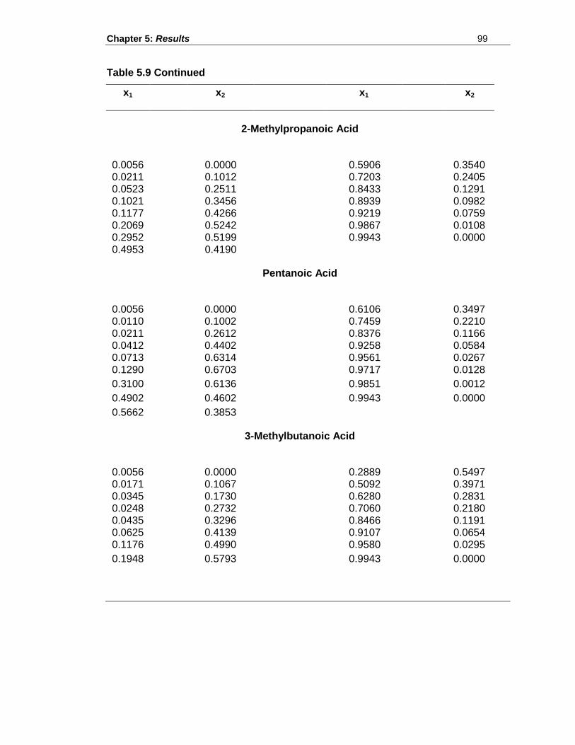
Chapter 5: Results 99
Table 5.9 Continued
x1
x2
x1
x2
2-Methylpropanoic Acid
0.0056
0.0000
0.5906
0.3540 0.0211
0.1012
0.7203
0.2405
0.0523
0.2511
0.8433
0.1291 0.1021
0.3456
0.8939
0.0982
0.1177
0.4266
0.9219
0.0759 0.2069
0.5242
0.9867
0.0108
0.2952
0.5199
0.9943
0.0000 0.4953
0.4190
Pentanoic Acid
0.0056
0.0000
0.6106
0.3497 0.0110
0.1002
0.7459
0.2210
0.0211
0.2612
0.8376
0.1166 0.0412
0.4402
0.9258
0.0584
0.0713
0.6314
0.9561
0.0267
0.1290
0.6703
0.9717
0.0128
0.3100
0.6136
0.9851
0.0012
0.4902
0.4602
0.9943
0.0000
0.5662
0.3853
3-Methylbutanoic Acid
0.0056
0.0000
0.2889
0.5497 0.0171
0.1067
0.5092
0.3971
0.0345
0.1730
0.6280
0.2831 0.0248
0.2732
0.7060
0.2180
0.0435
0.3296
0.8466
0.1191 0.0625
0.4139
0.9107
0.0654
0.1176
0.4990
0.9580
0.0295
0.1948
0.5793
0.9943
0.0000
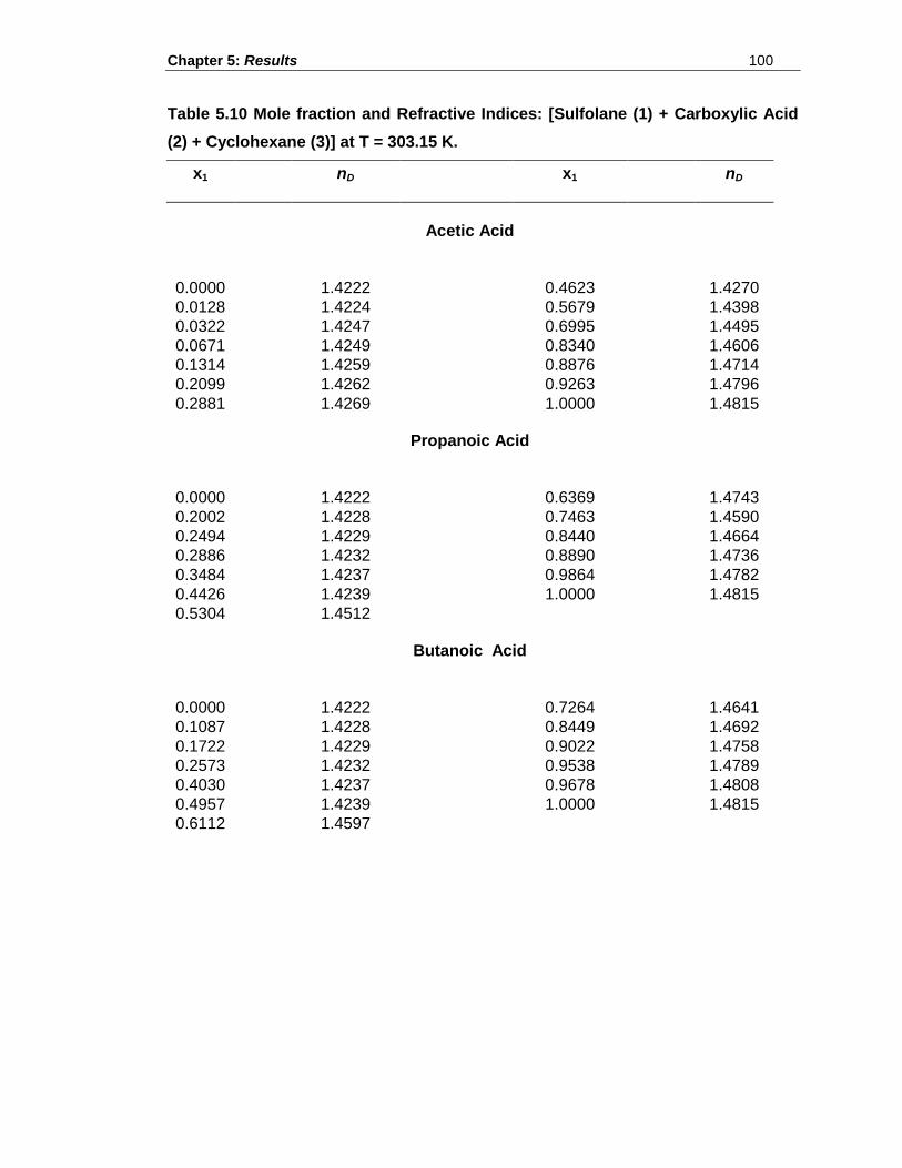
Chapter 5: Results 100
Table 5.10 Mole fraction and Refractive Indices: [Sulfolane (1) + Carboxylic Acid
(2) + Cyclohexane (3)] at T = 303.15 K.
x1
nD
x1
nD
Acetic Acid
0.0000
1.4222
0.4623
1.4270
0.0128
1.4224
0.5679
1.4398
0.0322
1.4247
0.6995
1.4495
0.0671
1.4249
0.8340
1.4606
0.1314
1.4259
0.8876
1.4714
0.2099
1.4262
0.9263
1.4796
0.2881
1.4269
1.0000
1.4815
Propanoic Acid
0.0000
1.4222
0.6369
1.4743
0.2002
1.4228
0.7463
1.4590
0.2494
1.4229
0.8440
1.4664
0.2886
1.4232
0.8890
1.4736
0.3484
1.4237
0.9864
1.4782
0.4426
1.4239
1.0000
1.4815
0.5304
1.4512
Butanoic Acid
0.0000
1.4222
0.7264
1.4641
0.1087
1.4228
0.8449
1.4692
0.1722
1.4229
0.9022
1.4758
0.2573
1.4232
0.9538
1.4789
0.4030
1.4237
0.9678
1.4808
0.4957
1.4239
1.0000
1.4815
0.6112
1.4597
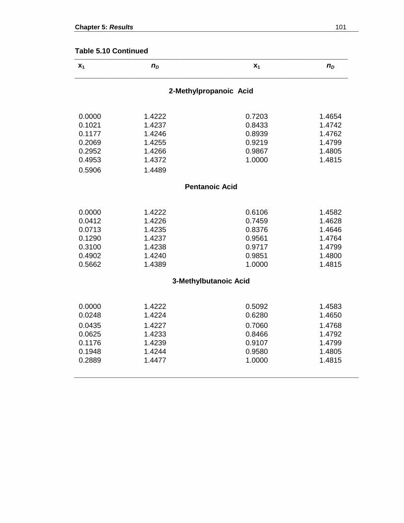
Chapter 5: Results 101
Table 5.10 Continued
x1
nD
x1
nD
2-Methylpropanoic Acid
0.0000
1.4222
0.7203
1.4654
0.1021
1.4237
0.8433
1.4742
0.1177
1.4246
0.8939
1.4762
0.2069
1.4255
0.9219
1.4799
0.2952
1.4266
0.9867
1.4805
0.4953
1.4372
1.0000
1.4815
0.5906
1.4489
Pentanoic Acid
0.0000
1.4222
0.6106
1.4582
0.0412
1.4226
0.7459
1.4628
0.0713
1.4235
0.8376
1.4646
0.1290
1.4237
0.9561
1.4764
0.3100
1.4238
0.9717
1.4799
0.4902
1.4240
0.9851
1.4800
0.5662
1.4389
1.0000
1.4815
3-Methylbutanoic Acid
0.0000
1.4222
0.5092
1.4583
0.0248
1.4224
0.6280
1.4650
0.0435
1.4227
0.7060
1.4768
0.0625
1.4233
0.8466
1.4792
0.1176
1.4239
0.9107
1.4799
0.1948
1.4244
0.9580
1.4805
0.2889
1.4477
1.0000
1.4815
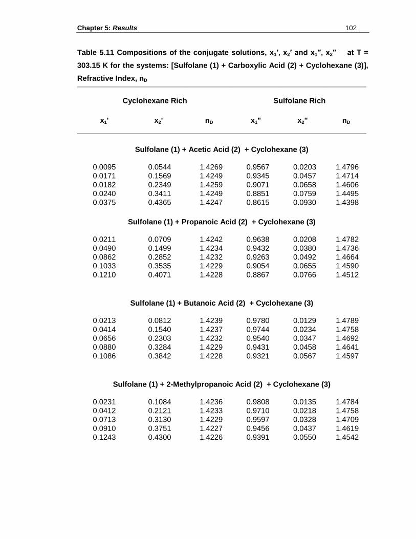
Chapter 5: Results 102
Table 5.11 Compositions of the conjugate solutions, x1′, x2′ and x1″, x2″ at T =
303.15 K for the systems: [Sulfolane (1) + Carboxylic Acid (2) + Cyclohexane (3)],
Refractive Index, nD
Cyclohexane Rich Sulfolane Rich
x1' x2' nD x1" x2" nD
Sulfolane (1) + Acetic Acid (2) + Cyclohexane (3)
0.0095 0.0544 1.4269 0.9567 0.0203 1.4796
0.0171 0.1569 1.4249 0.9345 0.0457 1.4714
0.0182 0.2349 1.4259 0.9071 0.0658 1.4606
0.0240 0.3411 1.4249 0.8851 0.0759 1.4495
0.0375 0.4365 1.4247 0.8615 0.0930 1.4398
Sulfolane (1) + Propanoic Acid (2) + Cyclohexane (3)
0.0211 0.0709 1.4242 0.9638 0.0208 1.4782
0.0490 0.1499 1.4234 0.9432 0.0380 1.4736
0.0862 0.2852 1.4232 0.9263 0.0492 1.4664
0.1033 0.3535 1.4229 0.9054 0.0655 1.4590
0.1210 0.4071 1.4228 0.8867 0.0766 1.4512
Sulfolane (1) + Butanoic Acid (2) + Cyclohexane (3)
0.0213 0.0812 1.4239 0.9780 0.0129 1.4789
0.0414 0.1540 1.4237 0.9744 0.0234 1.4758
0.0656 0.2303 1.4232 0.9540 0.0347 1.4692
0.0880 0.3284 1.4229 0.9431 0.0458 1.4641
0.1086 0.3842 1.4228 0.9321 0.0567 1.4597
Sulfolane (1) + 2-Methylpropanoic Acid (2) + Cyclohexane (3)
0.0231 0.1084 1.4236 0.9808 0.0135 1.4784
0.0412 0.2121 1.4233 0.9710 0.0218 1.4758
0.0713 0.3130 1.4229 0.9597 0.0328 1.4709
0.0910 0.3751 1.4227 0.9456 0.0437 1.4619
0.1243 0.4300 1.4226 0.9391 0.0550 1.4542
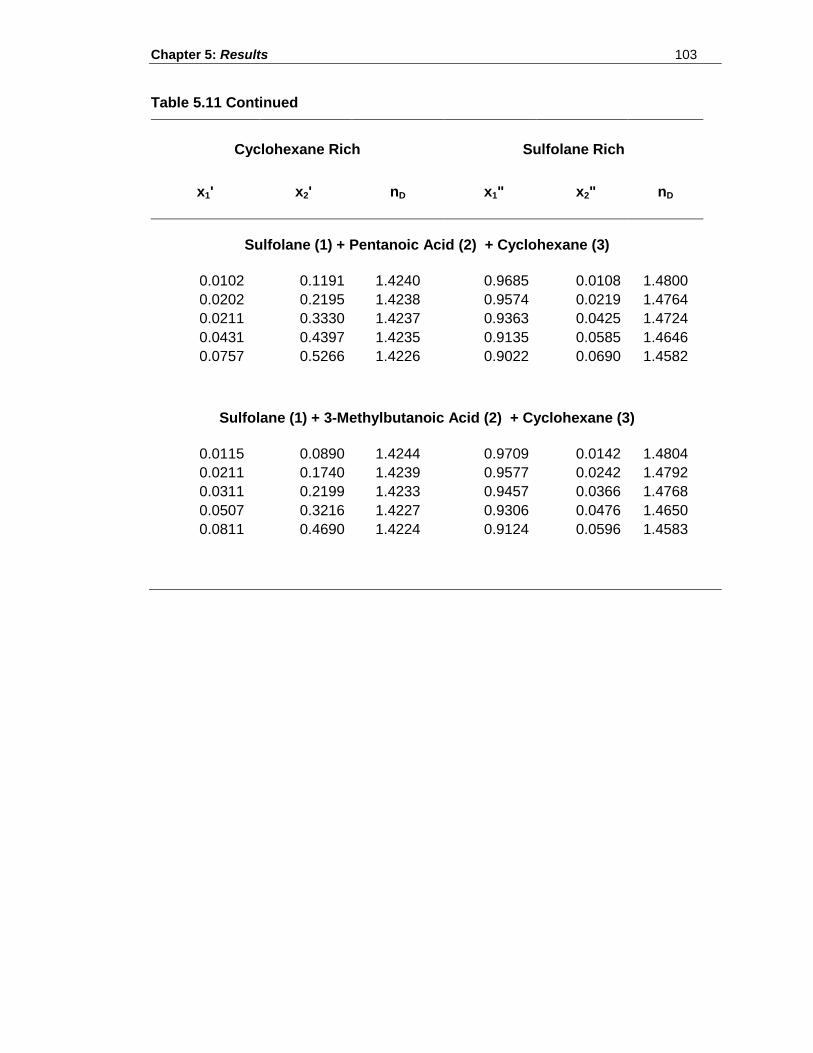
Chapter 5: Results 103
Table 5.11 Continued
Cyclohexane Rich Sulfolane Rich
x1' x2' nD x1" x2" nD
Sulfolane (1) + Pentanoic Acid (2) + Cyclohexane (3)
0.0102 0.1191 1.4240 0.9685 0.0108 1.4800
0.0202 0.2195 1.4238 0.9574 0.0219 1.4764
0.0211 0.3330 1.4237 0.9363 0.0425 1.4724
0.0431 0.4397 1.4235 0.9135 0.0585 1.4646
0.0757 0.5266 1.4226 0.9022 0.0690 1.4582
Sulfolane (1) + 3-Methylbutanoic Acid (2) + Cyclohexane (3)
0.0115 0.0890 1.4244 0.9709 0.0142 1.4804
0.0211 0.1740 1.4239 0.9577 0.0242 1.4792
0.0311 0.2199 1.4233 0.9457 0.0366 1.4768
0.0507 0.3216 1.4227 0.9306 0.0476 1.4650
0.0811 0.4690 1.4224 0.9124 0.0596 1.4583
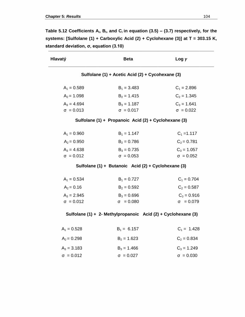
Chapter 5: Results 104
Table 5.12 Coefficients Ai, Bi, and Ci in equation (3.5) – (3.7) respectively, for the
systems: [Sulfolane (1) + Carboxylic Acid (2) + Cyclohexane (3)] at T = 303.15 K,
standard deviation, σ, equation (3.10)
Hlavatý
Beta
Log
Sulfolane (1) + Acetic Acid (2) + Cycohexane (3)
A1 = 0.589 B1 = 3.483 C1 = 2.896
A2 = 1.098 B2 = 1.415 C2 = 1.345
A3 = 4.694 B3 = 1.187 C3 = 1.641
σ = 0.013 σ = 0.017 σ = 0.022
Sulfolane (1) + Propanoic Acid (2) + Cyclohexane (3)
A1 = 0.960 B1 = 1.147 C1 =1.117
A2 = 0.950 B2 = 0.786 C2 = 0.781
A3 = 4.638 B3 = 0.735 C3 = 1.057
σ = 0.012 σ = 0.053 σ = 0.052
Sulfolane (1) + Butanoic Acid (2) + Cyclohexane (3)
A1 = 0.534 B1 = 0.727 C1 = 0.704
A2 = 0.16 B2 = 0.592 C2 = 0.587
A3 = 2.945 B3 = 0.696 C3 = 0.916
σ = 0.012 σ = 0.080
σ = 0.079
Sulfolane (1) + 2- Methylpropanoic Acid (2) + Cyclohexane (3)
A1 = 0.528 B1 = 6.157 C1 = 1.428
A2 = 0.298 B2 = 1.623 C2 = 0.834
A3 = 3.183 B3 = 1.466 C3 = 1.249
σ = 0.012 σ = 0.027 σ = 0.030
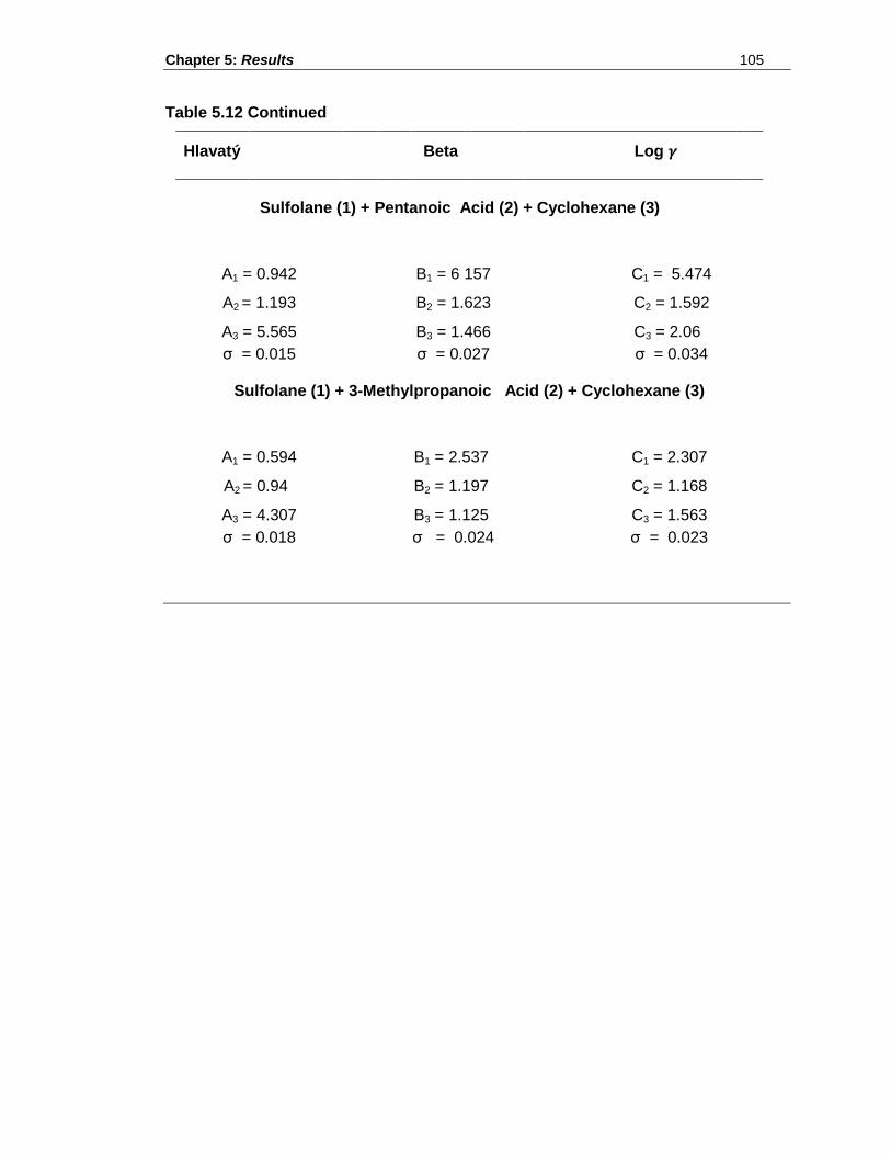
Chapter 5: Results 105
Table 5.12 Continued
Hlavatý
Beta
Log
Sulfolane (1) + Pentanoic Acid (2) + Cyclohexane (3)
A1 = 0.942 B1 = 6 157 C1 = 5.474
A2 = 1.193 B2 = 1.623 C2 = 1.592
A3 = 5.565 B3 = 1.466 C3 = 2.06
σ = 0.015 σ = 0.027 σ = 0.034
Sulfolane (1) + 3-Methylpropanoic Acid (2) + Cyclohexane (3)
A1 = 0.594 B1 = 2.537 C1 = 2.307
A2 = 0.94 B2 = 1.197 C2 = 1.168
A3 = 4.307 B3 = 1.125 C3 = 1.563 σ = 0.018 σ = 0.024 σ = 0.023
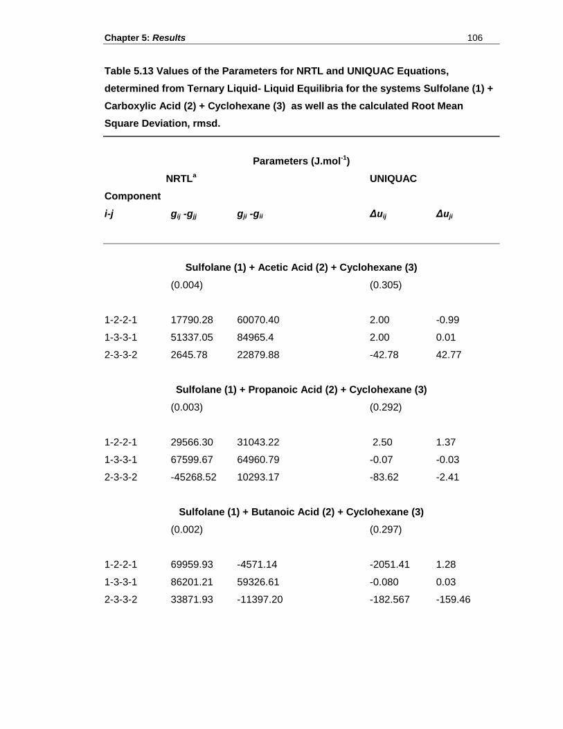
Chapter 5: Results 106
Table 5.13 Values of the Parameters for NRTL and UNIQUAC Equations,
determined from Ternary Liquid- Liquid Equilibria for the systems Sulfolane (1) +
Carboxylic Acid (2) + Cyclohexane (3) as well as the calculated Root Mean
Square Deviation, rmsd.
Parameters (J.mol-1)
NRTLa UNIQUAC
Component
i-j gij -gjj gji -gii Δuij Δuji
Sulfolane (1) + Acetic Acid (2) + Cyclohexane (3)
(0.004) (0.305)
1-2-2-1 17790.28 60070.40 2.00 -0.99
1-3-3-1 51337.05 84965.4 2.00 0.01
2-3-3-2 2645.78 22879.88 -42.78 42.77
Sulfolane (1) + Propanoic Acid (2) + Cyclohexane (3)
(0.003) (0.292)
1-2-2-1 29566.30 31043.22 2.50 1.37
1-3-3-1 67599.67 64960.79 -0.07 -0.03
2-3-3-2 -45268.52 10293.17 -83.62 -2.41
Sulfolane (1) + Butanoic Acid (2) + Cyclohexane (3)
(0.002) (0.297)
1-2-2-1 69959.93 -4571.14 -2051.41 1.28
1-3-3-1 86201.21 59326.61 -0.080 0.03
2-3-3-2 33871.93 -11397.20 -182.567 -159.46
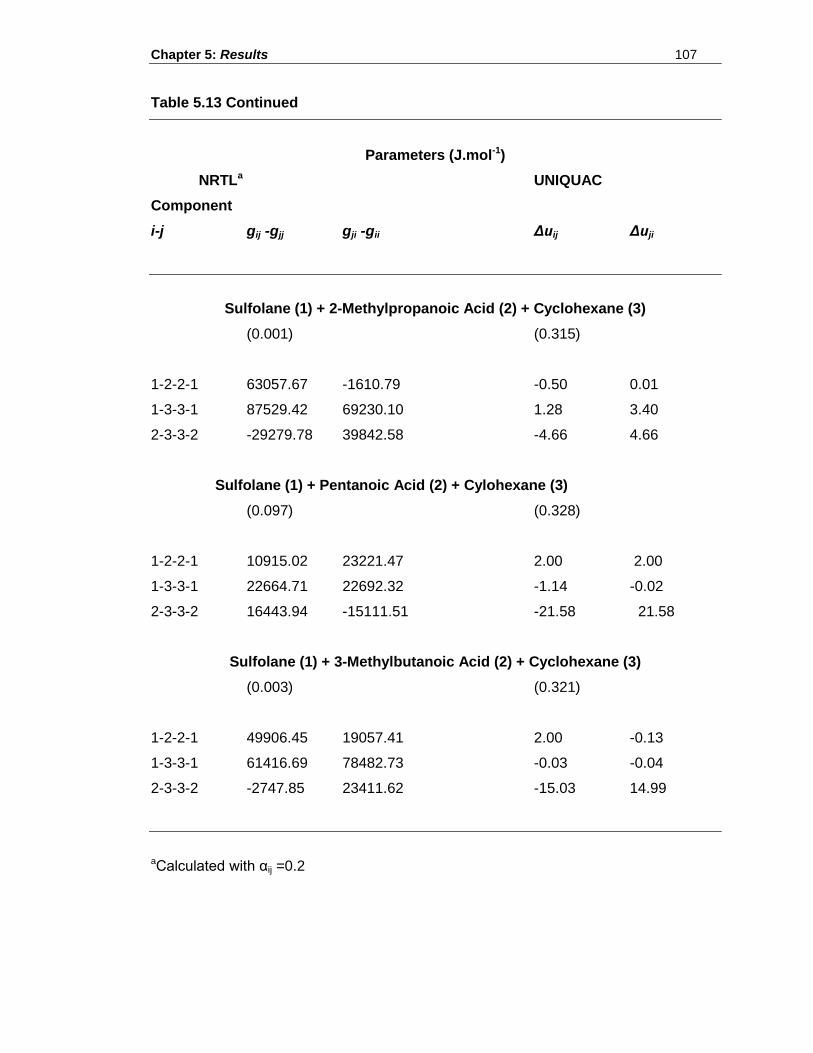
Chapter 5: Results 107
Table 5.13 Continued
Parameters (J.mol-1)
NRTLa UNIQUAC
Component
i-j gij -gjj gji -gii Δuij Δuji
Sulfolane (1) + 2-Methylpropanoic Acid (2) + Cyclohexane (3)
(0.001) (0.315)
1-2-2-1 63057.67 -1610.79 -0.50 0.01
1-3-3-1 87529.42 69230.10 1.28 3.40
2-3-3-2 -29279.78 39842.58 -4.66 4.66
Sulfolane (1) + Pentanoic Acid (2) + Cylohexane (3)
(0.097) (0.328)
1-2-2-1 10915.02 23221.47 2.00 2.00
1-3-3-1 22664.71 22692.32 -1.14 -0.02
2-3-3-2 16443.94 -15111.51 -21.58 21.58
Sulfolane (1) + 3-Methylbutanoic Acid (2) + Cyclohexane (3)
(0.003) (0.321)
1-2-2-1 49906.45 19057.41 2.00 -0.13
1-3-3-1 61416.69 78482.73 -0.03 -0.04
2-3-3-2 -2747.85 23411.62 -15.03 14.99
aCalculated with αij =0.2
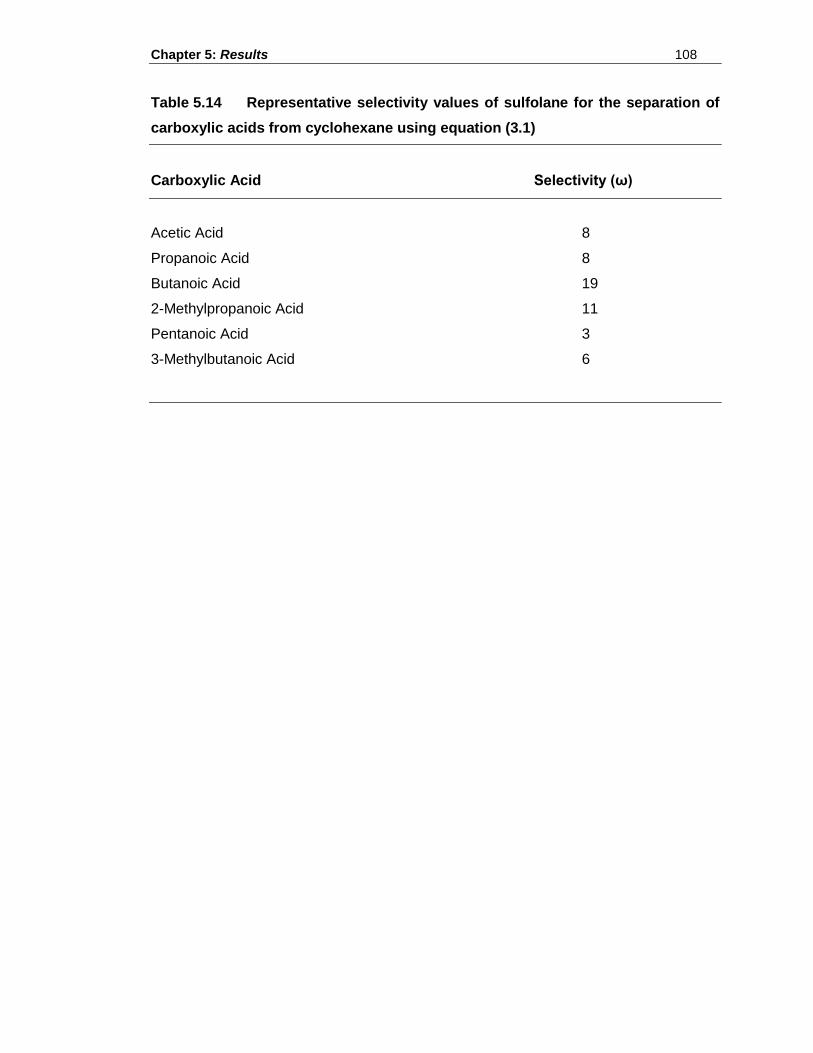
Chapter 5: Results 108
Table 5.14 Representative selectivity values of sulfolane for the separation of
carboxylic acids from cyclohexane using equation (3.1)
Carboxylic Acid Selectivity (ω)
Acetic Acid 8
Propanoic Acid 8
Butanoic Acid 19
2-Methylpropanoic Acid 11
Pentanoic Acid 3
3-Methylbutanoic Acid 6
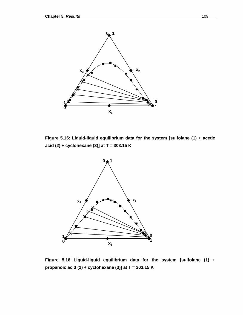
Chapter 5: Results 109
Figure 5.15: Liquid-liquid equilibrium data for the system [sulfolane (1) + acetic
acid (2) + cyclohexane (3)] at T = 303.15 K
Figure 5.16 Liquid-liquid equilibrium data for the system [sulfolane (1) +
propanoic acid (2) + cyclohexane (3)] at T = 303.15 K
1 0
0 1
0 1
x2 x3
x1
1 0
0 1
x3 x2
x1
0 1
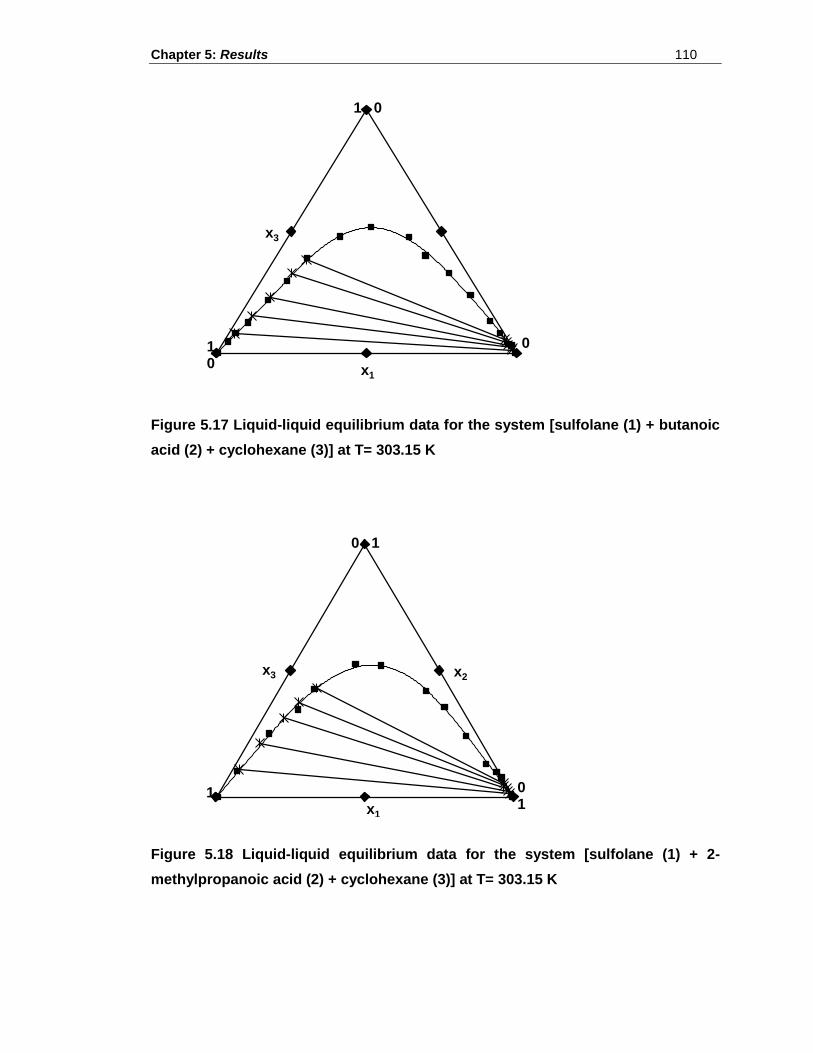
Chapter 5: Results 110
Figure 5.17 Liquid-liquid equilibrium data for the system [sulfolane (1) + butanoic
acid (2) + cyclohexane (3)] at T= 303.15 K
Figure 5.18 Liquid-liquid equilibrium data for the system [sulfolane (1) + 2-
methylpropanoic acid (2) + cyclohexane (3)] at T= 303.15 K
0 1 0
x3
x1
1 0
x3 x2
x1
0 1
0 1
1
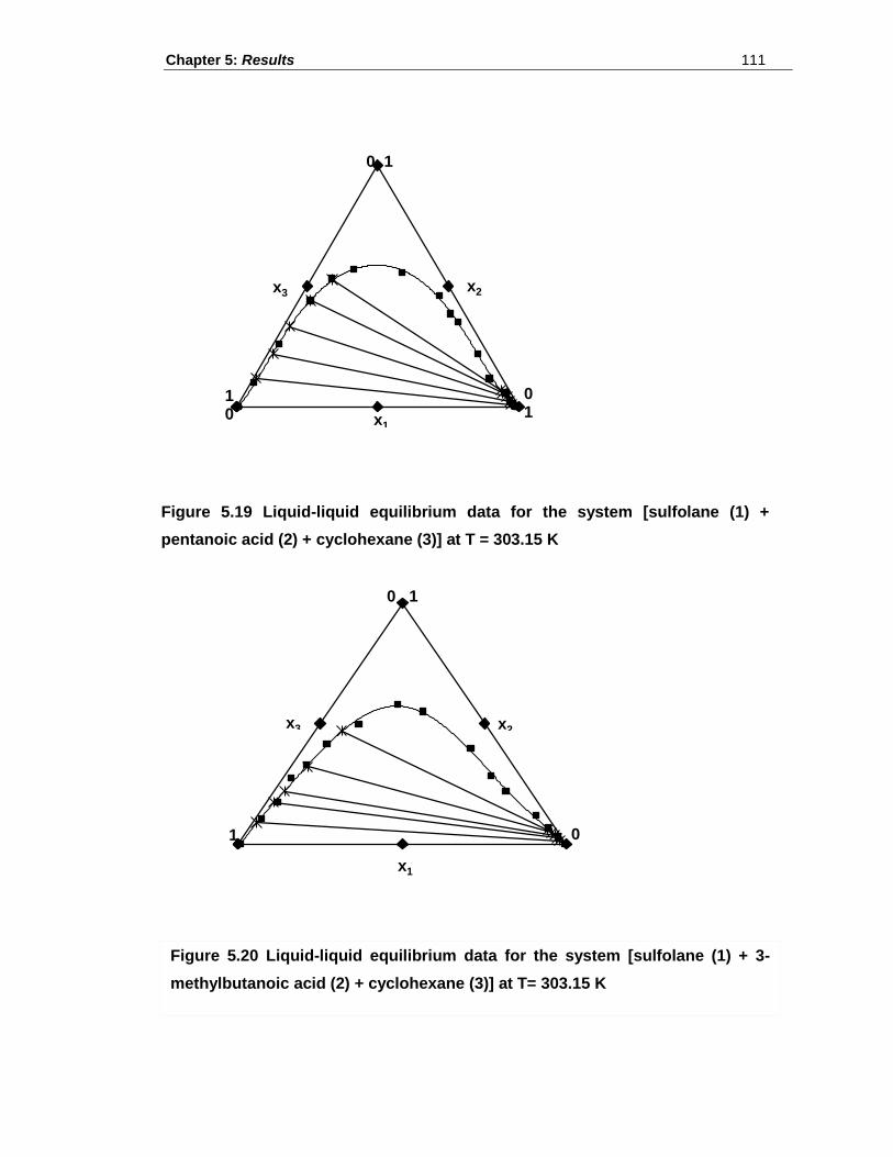
Chapter 5: Results 111
0 1
1 0
0 1
x2 x3
x1
1
0 1
x3 x2
x1
0
Figure 5.20 Liquid-liquid equilibrium data for the system [sulfolane (1) + 3-
methylbutanoic acid (2) + cyclohexane (3)] at T= 303.15 K
Figure 5.19 Liquid-liquid equilibrium data for the system [sulfolane (1) +
pentanoic acid (2) + cyclohexane (3)] at T = 303.15 K
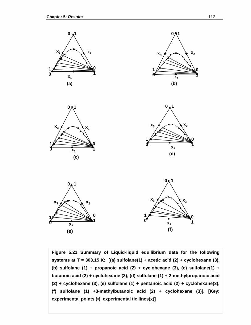
Chapter 5: Results 112
1 0
0 1
0 1
x2 x3
x1
1 0
0 1
x3 x2
x1
0 1
0 1
1 0
x3 x2
x1
0 1
x3 x2
x1
0 1
0 1
1 0
0 1
1 0
0 1
x2 x3
x1
1 0
0 1
x3 x2
x1
0 1
(e) (f)
(d) (c)
(a) (b)
Figure 5.21 Summary of Liquid-liquid equilibrium data for the following
systems at T = 303.15 K: [(a) sulfolane(1) + acetic acid (2) + cyclohexane (3),
(b) sulfolane (1) + propanoic acid (2) + cyclohexane (3), (c) sulfolane(1) +
butanoic acid (2) + cyclohexane (3), (d) sulfolane (1) + 2-methylpropanoic acid
(2) + cyclohexane (3), (e) sulfolane (1) + pentanoic acid (2) + cyclohexane(3),
(f) sulfolane (1) +3-methylbutanoic acid (2) + cyclohexane (3)]. [Key:
experimental points (▪), experimental tie lines(x)]
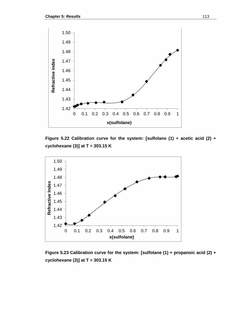
Chapter 5: Results 113
Figure 5.22 Calibration curve for the system: [sulfolane (1) + acetic acid (2) +
cyclohexane (3)] at T = 303.15 K
Figure 5.23 Calibration curve for the system: [sulfolane (1) + propanoic acid (2) +
cyclohexane (3)] at T = 303.15 K
1.42
1.43
1.44
1.45
1.46
1.47
1.48
1.49
1.50
0 0.1 0.2 0.3 0.4 0.5 0.6 0.7 0.8 0.9 1
Re
fra
cti
ve
in
de
x
x(sulfolane)
1.42
1.43
1.44
1.45
1.46
1.47
1.48
1.49
1.50
0 0.1 0.2 0.3 0.4 0.5 0.6 0.7 0.8 0.9 1
Re
fra
cti
ve
In
de
x
x(sulfolane)
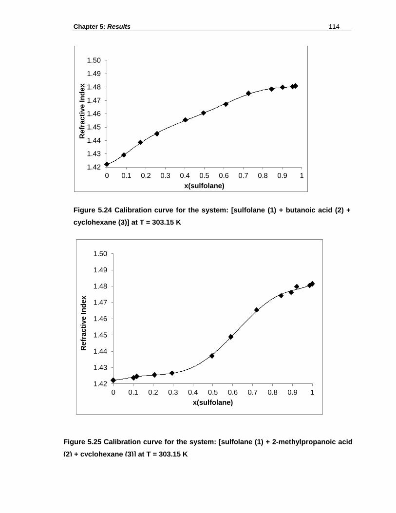
Chapter 5: Results 114
Figure 5.24 Calibration curve for the system: [sulfolane (1) + butanoic acid (2) +
cyclohexane (3)] at T = 303.15 K
1.42
1.43
1.44
1.45
1.46
1.47
1.48
1.49
1.50
0 0.1 0.2 0.3 0.4 0.5 0.6 0.7 0.8 0.9 1
Re
fra
cti
ve
In
de
x
x(sulfolane)
1.42
1.43
1.44
1.45
1.46
1.47
1.48
1.49
1.50
0 0.1 0.2 0.3 0.4 0.5 0.6 0.7 0.8 0.9 1
Re
fra
cti
ve
In
de
x
x(sulfolane)
Figure 5.25 Calibration curve for the system: [sulfolane (1) + 2-methylpropanoic acid
(2) + cyclohexane (3)] at T = 303.15 K
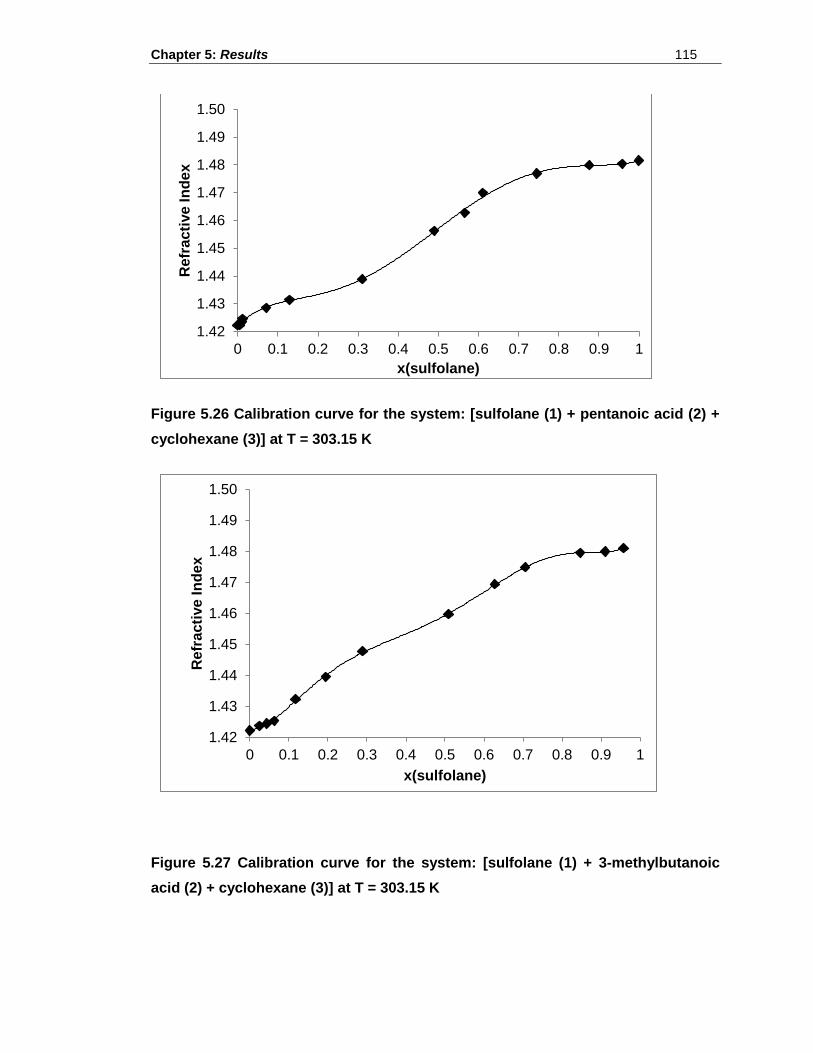
Chapter 5: Results 115
Figure 5.26 Calibration curve for the system: [sulfolane (1) + pentanoic acid (2) +
cyclohexane (3)] at T = 303.15 K
Figure 5.27 Calibration curve for the system: [sulfolane (1) + 3-methylbutanoic
acid (2) + cyclohexane (3)] at T = 303.15 K
1.42
1.43
1.44
1.45
1.46
1.47
1.48
1.49
1.50
0 0.1 0.2 0.3 0.4 0.5 0.6 0.7 0.8 0.9 1
Re
fra
cti
ve
In
de
x
x(sulfolane)
1.42
1.43
1.44
1.45
1.46
1.47
1.48
1.49
1.50
0 0.1 0.2 0.3 0.4 0.5 0.6 0.7 0.8 0.9 1
Re
fra
cti
ve
In
de
x
x(sulfolane)
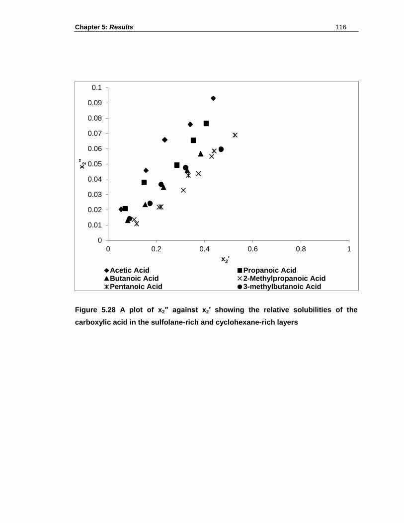
Chapter 5: Results 116
Figure 5.28 A plot of x2″ against x2′ showing the relative solubilities of the
carboxylic acid in the sulfolane-rich and cyclohexane-rich layers
0
0.01
0.02
0.03
0.04
0.05
0.06
0.07
0.08
0.09
0.1
0 0.2 0.4 0.6 0.8 1
x2"
x2'
Acetic Acid Propanoic AcidButanoic Acid 2-Methylpropanoic AcidPentanoic Acid 3-methylbutanoic Acid
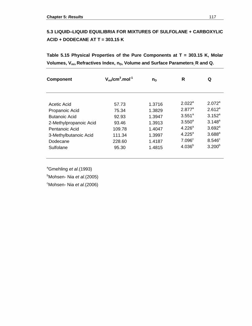
Chapter 5: Results 117
5.3 LIQUID–LIQUID EQUILIBRIA FOR MIXTURES OF SULFOLANE + CARBOXYLIC
ACID + DODECANE AT T = 303.15 K
Table 5.15 Physical Properties of the Pure Components at T = 303.15 K, Molar
Volumes, Vmi, Refractives Index, nD, Volume and Surface Parameters, R and Q.
Component Vmi/cm3.mol-1 nD R Q
Acetic Acid 57.73 1.3716 2.022a 2.072a
Propanoic Acid 75.34 1.3829 2.877a 2.612a
Butanoic Acid 92.93 1.3947 3.551a 3.152a
2-Methylpropanoic Acid 93.46 1.3913 3.550a 3.148a
Pentanoic Acid 109.78 1.4047 4.226a 3.692a
3-Methylbutanoic Acid 111.34 1.3997 4.225a 3.688a
Dodecane 228.60 1.4187 7.096c 8.546c
Sulfolane 95.30 1.4815 4.036b 3.200b
aGmehling et al.(1993)
bMohsen- Nia et al.(2005)
cMohsen- Nia et al.(2006)
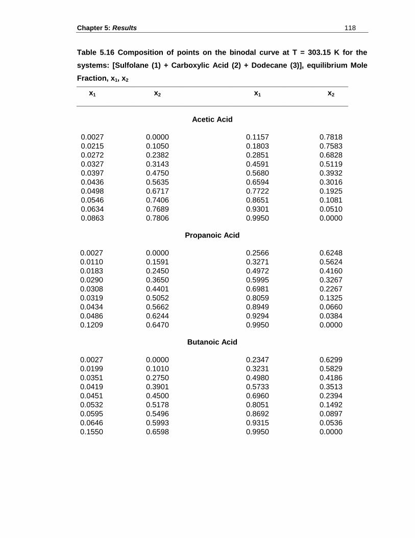
Chapter 5: Results 118
Table 5.16 Composition of points on the binodal curve at T = 303.15 K for the
systems: [Sulfolane (1) + Carboxylic Acid (2) + Dodecane (3)], equilibrium Mole
Fraction, x1, x2
x1
x2
x1
x2
Acetic Acid
0.0027
0.0000
0.1157
0.7818
0.0215
0.1050
0.1803
0.7583
0.0272
0.2382
0.2851
0.6828
0.0327
0.3143
0.4591
0.5119
0.0397
0.4750
0.5680
0.3932
0.0436
0.5635
0.6594
0.3016
0.0498
0.6717
0.7722
0.1925
0.0546
0.7406
0.8651
0.1081
0.0634
0.7689
0.9301
0.0510
0.0863
0.7806
0.9950
0.0000
Propanoic Acid
0.0027
0.0000
0.2566
0.6248
0.0110
0.1591
0.3271
0.5624
0.0183
0.2450
0.4972
0.4160
0.0290
0.3650
0.5995
0.3267
0.0308
0.4401
0.6981
0.2267
0.0319
0.5052
0.8059
0.1325
0.0434
0.5662
0.8949
0.0660
0.0486
0.6244
0.9294
0.0384
0.1209
0.6470
0.9950
0.0000
Butanoic Acid
0.0027
0.0000
0.2347
0.6299
0.0199
0.1010
0.3231
0.5829
0.0351
0.2750
0.4980
0.4186
0.0419
0.3901
0.5733
0.3513
0.0451
0.4500
0.6960
0.2394
0.0532
0.5178
0.8051
0.1492
0.0595
0.5496
0.8692
0.0897
0.0646
0.5993
0.9315
0.0536
0.1550
0.6598
0.9950
0.0000
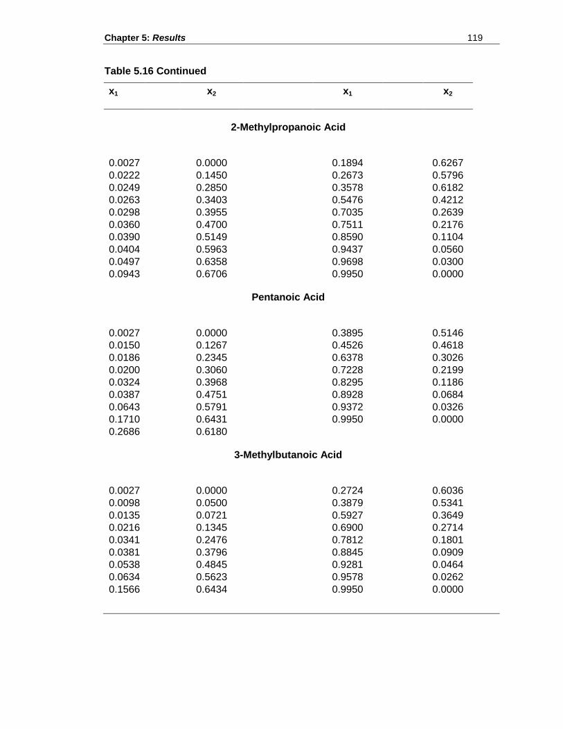
Chapter 5: Results 119
Table 5.16 Continued
x1
x2
x1
x2
2-Methylpropanoic Acid
0.0027
0.0000
0.1894
0.6267
0.0222
0.1450
0.2673
0.5796
0.0249
0.2850
0.3578
0.6182
0.0263
0.3403
0.5476
0.4212
0.0298
0.3955
0.7035
0.2639
0.0360
0.4700
0.7511
0.2176
0.0390
0.5149
0.8590
0.1104
0.0404
0.5963
0.9437
0.0560
0.0497
0.6358
0.9698
0.0300
0.0943
0.6706
0.9950
0.0000
Pentanoic Acid
0.0027
0.0000
0.3895
0.5146
0.0150
0.1267
0.4526
0.4618
0.0186
0.2345
0.6378
0.3026
0.0200
0.3060
0.7228
0.2199
0.0324
0.3968
0.8295
0.1186
0.0387
0.4751
0.8928
0.0684
0.0643
0.5791
0.9372
0.0326
0.1710
0.6431
0.9950
0.0000
0.2686
0.6180
3-Methylbutanoic Acid
0.0027
0.0000
0.2724
0.6036
0.0098
0.0500
0.3879
0.5341
0.0135
0.0721
0.5927
0.3649
0.0216
0.1345
0.6900
0.2714
0.0341
0.2476
0.7812
0.1801
0.0381
0.3796
0.8845
0.0909
0.0538
0.4845
0.9281
0.0464
0.0634
0.5623
0.9578
0.0262
0.1566
0.6434
0.9950
0.0000
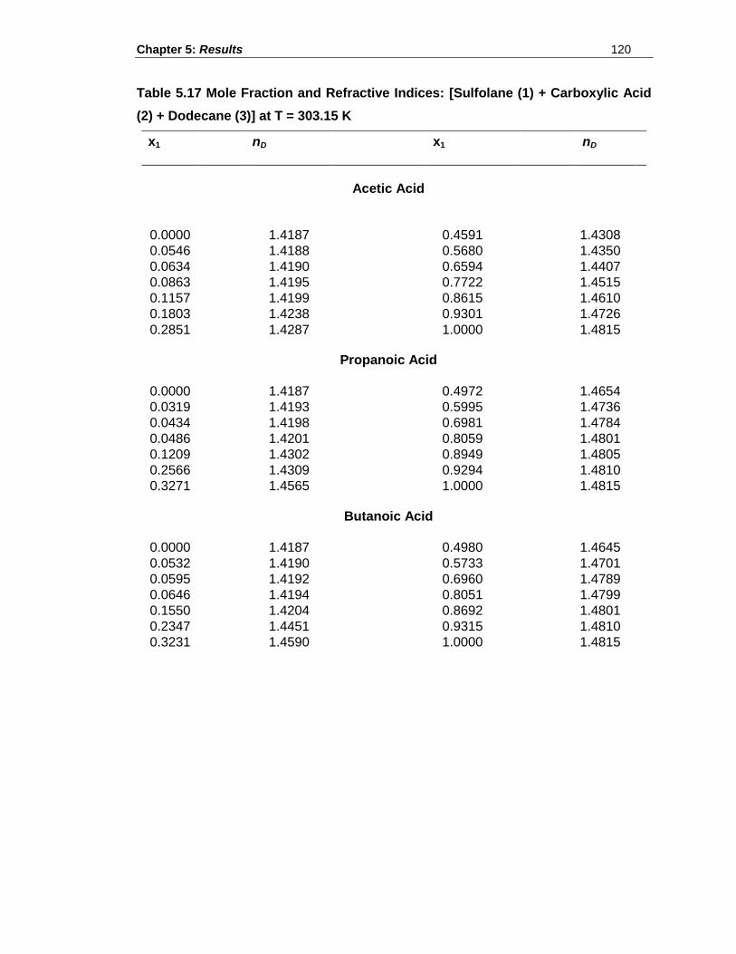
Chapter 5: Results 120
Table 5.17 Mole Fraction and Refractive Indices: [Sulfolane (1) + Carboxylic Acid
(2) + Dodecane (3)] at T = 303.15 K
x1 nD x1 nD
Acetic Acid
0.0000
1.4187
0.4591
1.4308
0.0546
1.4188
0.5680
1.4350
0.0634
1.4190
0.6594
1.4407
0.0863
1.4195
0.7722
1.4515
0.1157
1.4199
0.8615
1.4610
0.1803
1.4238
0.9301
1.4726
0.2851
1.4287
1.0000
1.4815
Propanoic Acid
0.0000
1.4187
0.4972
1.4654
0.0319
1.4193
0.5995
1.4736
0.0434
1.4198
0.6981
1.4784
0.0486
1.4201
0.8059
1.4801
0.1209
1.4302
0.8949
1.4805
0.2566
1.4309
0.9294
1.4810
0.3271
1.4565
1.0000
1.4815
Butanoic Acid
0.0000
1.4187
0.4980
1.4645
0.0532
1.4190
0.5733
1.4701
0.0595
1.4192
0.6960
1.4789
0.0646
1.4194
0.8051
1.4799
0.1550
1.4204
0.8692
1.4801
0.2347
1.4451
0.9315
1.4810
0.3231
1.4590
1.0000
1.4815
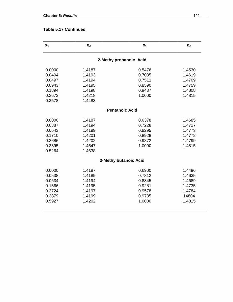
Chapter 5: Results 121
Table 5.17 Continued
x1
nD
x1
nD
2-Methylpropanoic Acid
0.0000
1.4187
0.5476
1.4530
0.0404
1.4193
0.7035
1.4619
0.0497
1.4194
0.7511
1.4709
0.0943
1.4195
0.8590
1.4759
0.1894
1.4198
0.9437
1.4808
0.2673
1.4218
1.0000
1.4815
0.3578
1.4483
Pentanoic Acid
0.0000
1.4187
0.6378
1.4685
0.0387
1.4194
0.7228
1.4727
0.0643
1.4199
0.8295
1.4773
0.1710
1.4201
0.8928
1.4778
0.3686
1.4202
0.9372
1.4799
0.3895
1.4547
1.0000
1.4815
0.5264
1.4638
3-Methylbutanoic Acid
0.0000
1.4187
0.6900
1.4496
0.0538
1.4189
0.7812
1.4635
0.0634
1.4194
0.8845
1.4689
0.1566
1.4195
0.9281
1.4735
0.2724
1.4197
0.9578
1.4784
0.3879
1.4199
0.9735
14804
0.5927
1.4202
1.0000
1.4815
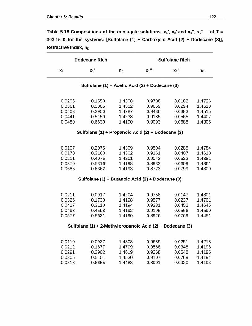
Chapter 5: Results 122
Table 5.18 Compositions of the conjugate solutions, x1′, x2′ and x1″, x2″ at T =
303.15 K for the systems: [Sulfolane (1) + Carboxylic Acid (2) + Dodecane (3)],
Refractive Index, nD
Dodecane Rich Sulfolane Rich
x1' x2' nD x1" x2" nD
Sulfolane (1) + Acetic Acid (2) + Dodecane (3)
0.0206 0.1550 1.4308 0.9708 0.0182 1.4726 0.0361 0.3005 1.4302 0.9659 0.0294 1.4610 0.0403 0.3950 1.4287 0.9436 0.0383 1.4515 0.0441 0.5150 1.4238 0.9185 0.0565 1.4407 0.0480 0.6630 1.4190 0.9093 0.0688 1.4305
Sulfolane (1) + Propanoic Acid (2) + Dodecane (3)
0.0107 0.2075 1.4309 0.9504 0.0285 1.4784 0.0170 0.3163 1.4302 0.9161 0.0407 1.4610 0.0211 0.4075 1.4201 0.9043 0.0522 1.4381 0.0370 0.5316 1.4198 0.8933 0.0609 1.4361 0.0685 0.6362 1.4193 0.8723 0.0799 1.4309
Sulfolane (1) + Butanoic Acid (2) + Dodecane (3)
0.0211 0.0917 1.4204 0.9758 0.0147 1.4801 0.0326 0.1730 1.4198 0.9577 0.0237 1.4701 0.0417 0.3110 1.4194 0.9281 0.0452 1.4645 0.0493 0.4598 1.4192 0.9195 0.0566 1.4590 0.0577 0.5621 1.4190 0.8926 0.0769 1.4451
Sulfolane (1) + 2-Methylpropanoic Acid (2) + Dodecane (3)
0.0110 0.0927 1.4808 0.9689 0.0251 1.4218 0.0212 0.1877 1.4709 0.9568 0.0348 1.4198 0.0291 0.2902 1.4619 0.9368 0.0548 1.4195 0.0305 0.5101 1.4530 0.9107 0.0769 1.4194 0.0318 0.6655 1.4483 0.8901 0.0920 1.4193
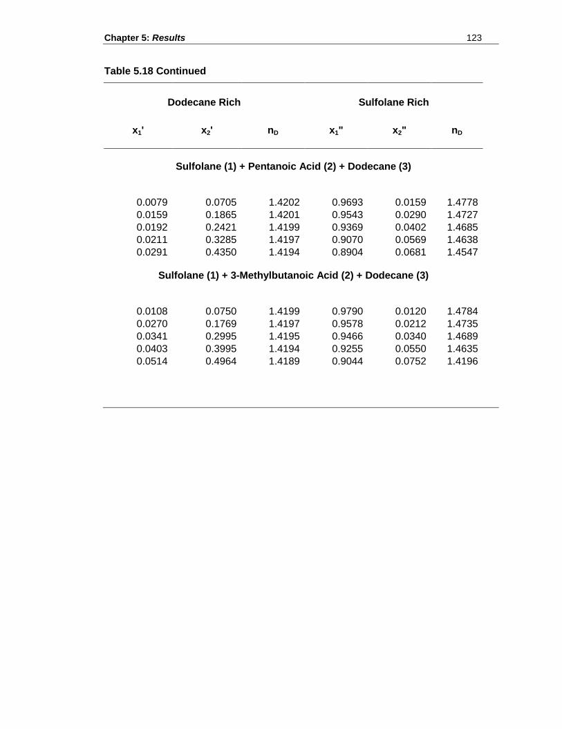
Chapter 5: Results 123
Table 5.18 Continued
Dodecane Rich Sulfolane Rich
x1' x2' nD x1" x2" nD
Sulfolane (1) + Pentanoic Acid (2) + Dodecane (3)
0.0079 0.0705 1.4202 0.9693 0.0159 1.4778
0.0159 0.1865 1.4201 0.9543 0.0290 1.4727
0.0192 0.2421 1.4199 0.9369 0.0402 1.4685
0.0211 0.3285 1.4197 0.9070 0.0569 1.4638
0.0291 0.4350 1.4194 0.8904 0.0681 1.4547
Sulfolane (1) + 3-Methylbutanoic Acid (2) + Dodecane (3)
0.0108 0.0750 1.4199 0.9790 0.0120 1.4784
0.0270 0.1769 1.4197 0.9578 0.0212 1.4735
0.0341 0.2995 1.4195 0.9466 0.0340 1.4689
0.0403 0.3995 1.4194 0.9255 0.0550 1.4635
0.0514 0.4964 1.4189 0.9044 0.0752 1.4196
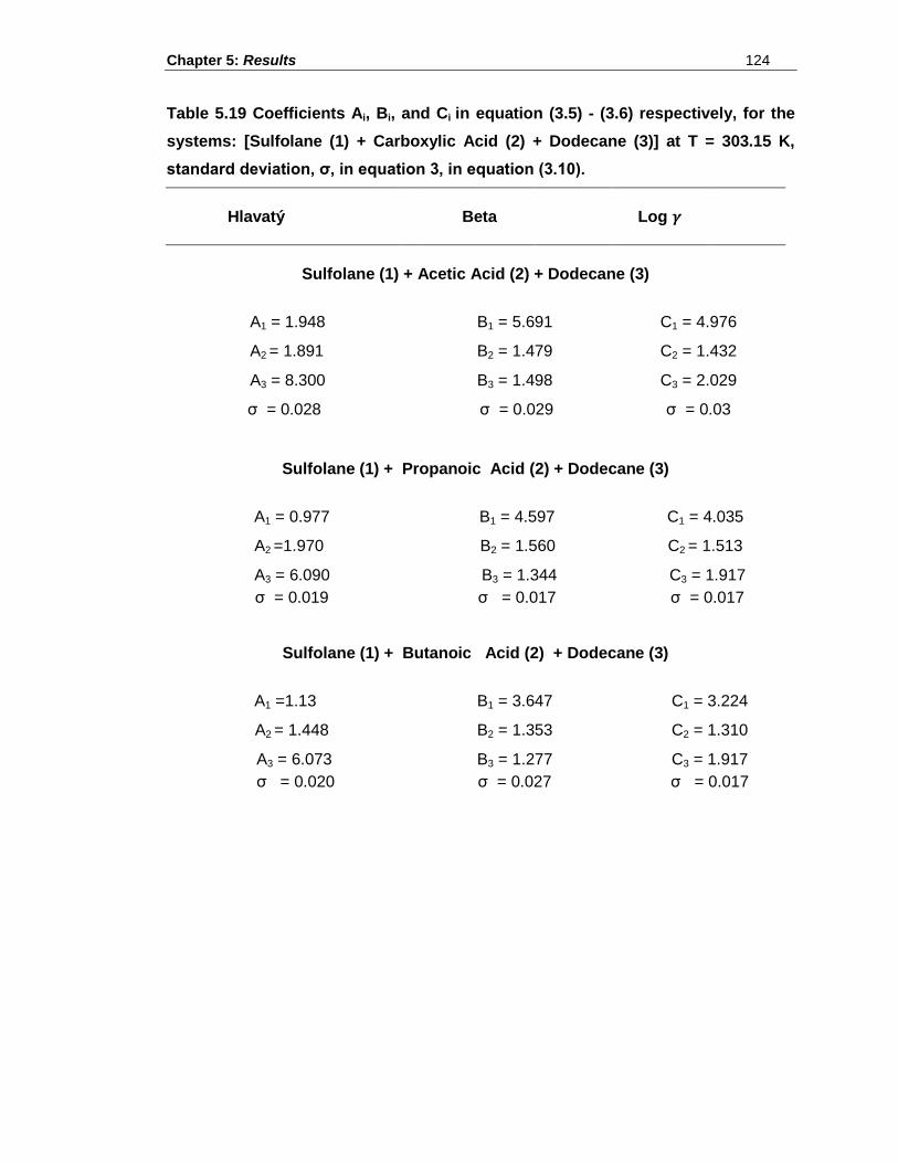
Chapter 5: Results 124
Table 5.19 Coefficients Ai, Bi, and Ci in equation (3.5) - (3.6) respectively, for the
systems: [Sulfolane (1) + Carboxylic Acid (2) + Dodecane (3)] at T = 303.15 K,
standard deviation, σ, in equation 3, in equation (3.10).
Hlavatý
Beta
Log
Sulfolane (1) + Acetic Acid (2) + Dodecane (3)
A1 = 1.948 B1 = 5.691 C1 = 4.976
A2 = 1.891 B2 = 1.479 C2 = 1.432
A3 = 8.300
B3 = 1.498 C3 = 2.029
σ = 0.028
σ = 0.029 σ = 0.03
Sulfolane (1) + Propanoic Acid (2) + Dodecane (3)
A1 = 0.977 B1 = 4.597 C1 = 4.035
A2 =1.970 B2 = 1.560 C2 = 1.513
A3 = 6.090 B3 = 1.344 C3 = 1.917
σ = 0.019 σ = 0.017 σ = 0.017
Sulfolane (1) + Butanoic Acid (2) + Dodecane (3)
A1 =1.13 B1 = 3.647 C1 = 3.224
A2 = 1.448 B2 = 1.353 C2 = 1.310
A3 = 6.073 B3 = 1.277 C3 = 1.917
σ = 0.020
σ = 0.027 σ = 0.017
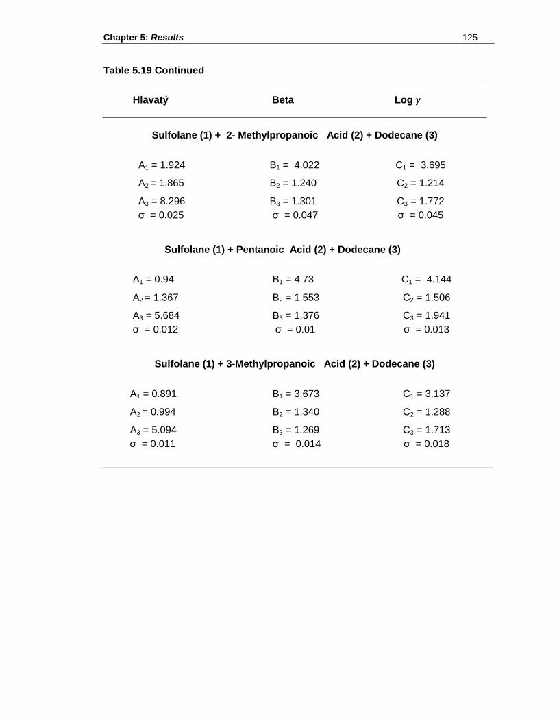
Chapter 5: Results 125
Table 5.19 Continued
Hlavatý
Beta
Log
Sulfolane (1) + 2- Methylpropanoic Acid (2) + Dodecane (3)
A1 = 1.924 B1 = 4.022 C1 = 3.695
A2 = 1.865 B2 = 1.240 C2 = 1.214
A3 = 8.296 B3 = 1.301 C3 = 1.772 σ = 0.025 σ = 0.047 σ = 0.045
Sulfolane (1) + Pentanoic Acid (2) + Dodecane (3)
A1 = 0.94 B1 = 4.73 C1 = 4.144
A2 = 1.367 B2 = 1.553 C2 = 1.506
A3 = 5.684 B3 = 1.376 C3 = 1.941 σ = 0.012 σ = 0.01
σ = 0.013
Sulfolane (1) + 3-Methylpropanoic Acid (2) + Dodecane (3)
A1 = 0.891 B1 = 3.673 C1 = 3.137
A2 = 0.994 B2 = 1.340 C2 = 1.288
A3 = 5.094 B3 = 1.269 C3 = 1.713 σ = 0.011 σ = 0.014 σ = 0.018
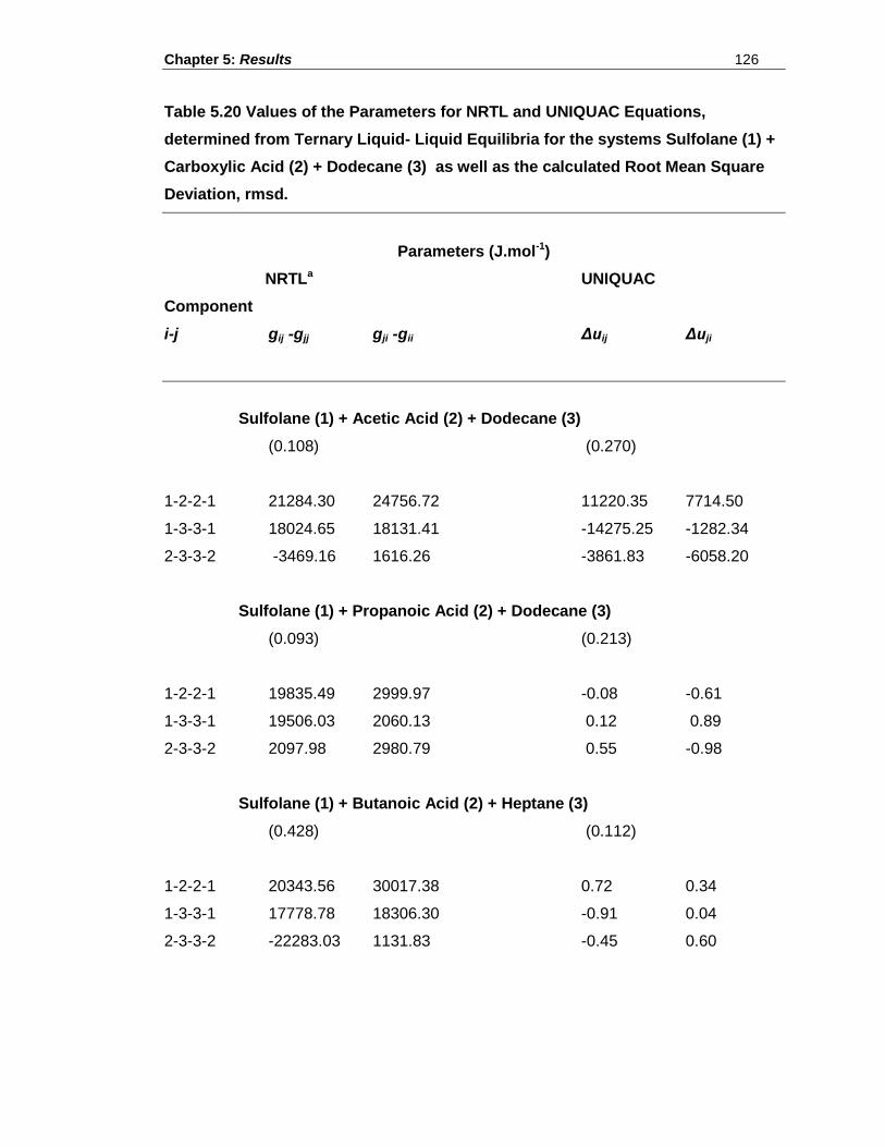
Chapter 5: Results 126
Table 5.20 Values of the Parameters for NRTL and UNIQUAC Equations,
determined from Ternary Liquid- Liquid Equilibria for the systems Sulfolane (1) +
Carboxylic Acid (2) + Dodecane (3) as well as the calculated Root Mean Square
Deviation, rmsd.
Parameters (J.mol-1)
NRTLa UNIQUAC
Component
i-j gij -gjj gji -gii Δuij Δuji
Sulfolane (1) + Acetic Acid (2) + Dodecane (3)
(0.108) (0.270)
1-2-2-1 21284.30 24756.72 11220.35 7714.50
1-3-3-1 18024.65 18131.41 -14275.25 -1282.34
2-3-3-2 -3469.16 1616.26 -3861.83 -6058.20
Sulfolane (1) + Propanoic Acid (2) + Dodecane (3)
(0.093) (0.213)
1-2-2-1 19835.49 2999.97 -0.08 -0.61
1-3-3-1 19506.03 2060.13 0.12 0.89
2-3-3-2 2097.98 2980.79 0.55 -0.98
Sulfolane (1) + Butanoic Acid (2) + Heptane (3)
(0.428) (0.112)
1-2-2-1 20343.56 30017.38 0.72 0.34
1-3-3-1 17778.78 18306.30 -0.91 0.04
2-3-3-2 -22283.03 1131.83 -0.45 0.60
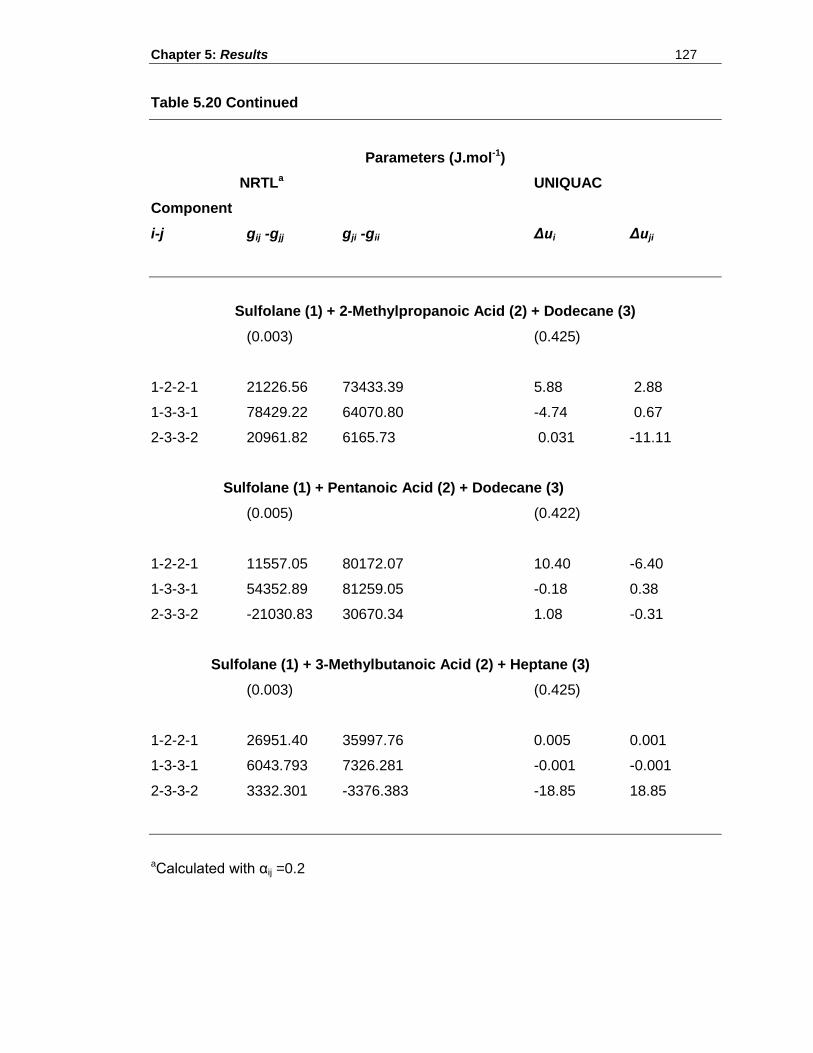
Chapter 5: Results 127
Table 5.20 Continued
Parameters (J.mol-1)
NRTLa UNIQUAC
Component
i-j gij -gjj gji -gii Δui Δuji
Sulfolane (1) + 2-Methylpropanoic Acid (2) + Dodecane (3)
(0.003) (0.425)
1-2-2-1 21226.56 73433.39 5.88 2.88
1-3-3-1 78429.22 64070.80 -4.74 0.67
2-3-3-2 20961.82 6165.73 0.031 -11.11
Sulfolane (1) + Pentanoic Acid (2) + Dodecane (3)
(0.005) (0.422)
1-2-2-1 11557.05 80172.07 10.40 -6.40
1-3-3-1 54352.89 81259.05 -0.18 0.38
2-3-3-2 -21030.83 30670.34 1.08 -0.31
Sulfolane (1) + 3-Methylbutanoic Acid (2) + Heptane (3)
(0.003) (0.425)
1-2-2-1 26951.40 35997.76 0.005 0.001
1-3-3-1 6043.793 7326.281 -0.001 -0.001
2-3-3-2 3332.301 -3376.383 -18.85 18.85
aCalculated with αij =0.2
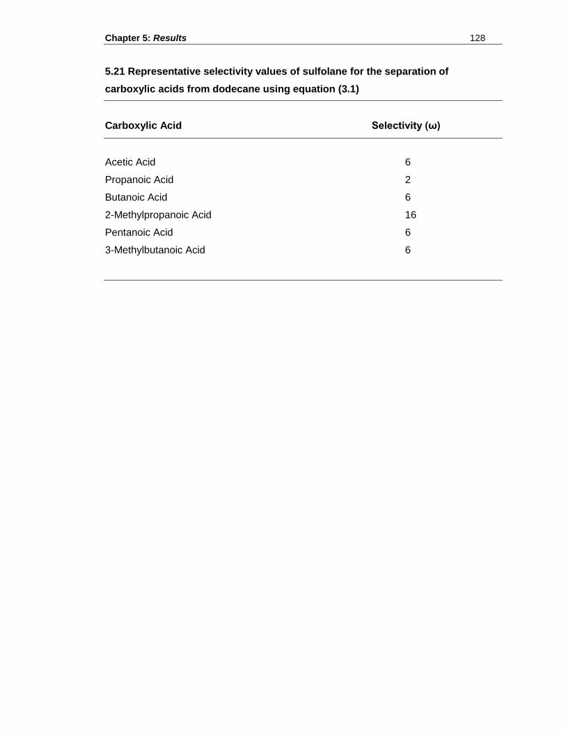
Chapter 5: Results 128
5.21 Representative selectivity values of sulfolane for the separation of
carboxylic acids from dodecane using equation (3.1)
Carboxylic Acid Selectivity (ω)
Acetic Acid 6
Propanoic Acid 2
Butanoic Acid 6
2-Methylpropanoic Acid 16
Pentanoic Acid 6
3-Methylbutanoic Acid 6
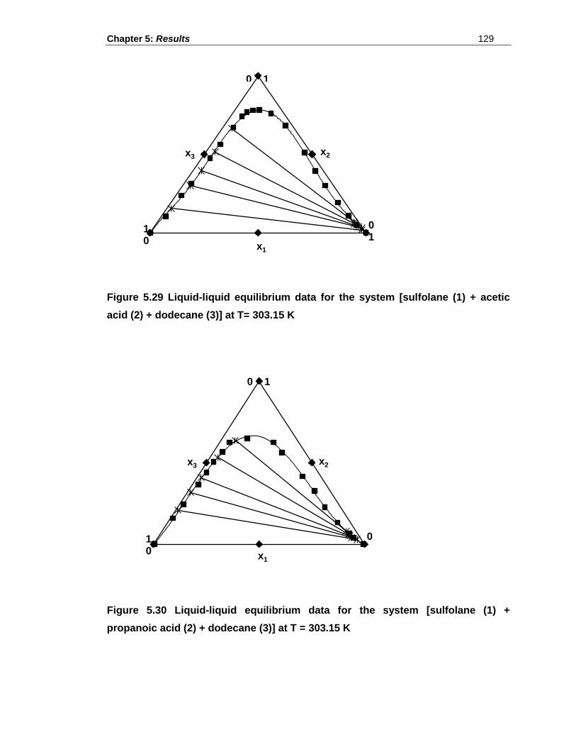
Chapter 5: Results 129
Figure 5.29 Liquid-liquid equilibrium data for the system [sulfolane (1) + acetic
acid (2) + dodecane (3)] at T= 303.15 K
Figure 5.30 Liquid-liquid equilibrium data for the system [sulfolane (1) +
propanoic acid (2) + dodecane (3)] at T = 303.15 K
x1
x3 x2
0 1
1 0
0 1
x3
x1
x2
0 1 0
0 1
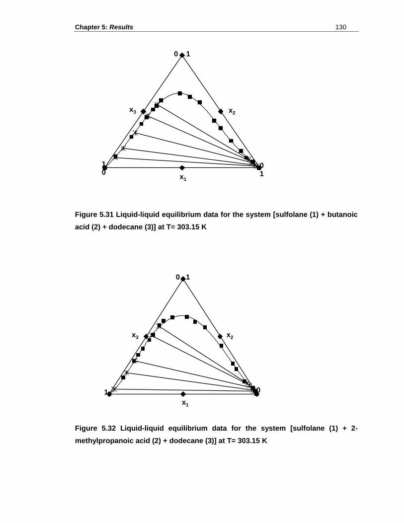
Chapter 5: Results 130
Figure 5.31 Liquid-liquid equilibrium data for the system [sulfolane (1) + butanoic
acid (2) + dodecane (3)] at T= 303.15 K
Figure 5.32 Liquid-liquid equilibrium data for the system [sulfolane (1) + 2-
methylpropanoic acid (2) + dodecane (3)] at T= 303.15 K
x2 x3
x1
0 1
1 0
0 1
x3 x2
x1
1 0
0 1
Chapter 5: Results 131
Figure 5.33 Liquid-liquid equilibrium data for the system [sulfolane (1) +
pentanoic acid (2) + dodecane (3)] at T= 303.15 K
Figure 5.34 Liquid-liquid equilibrium data for the system [sulfolane (1) + 3-
methylbutanoic acid (2) + dodecane (3)] at T= 303.15 K
0 1
x2 x3
x1
1 0
0 1
x2 x3
x1
0 1
1 0
0 1
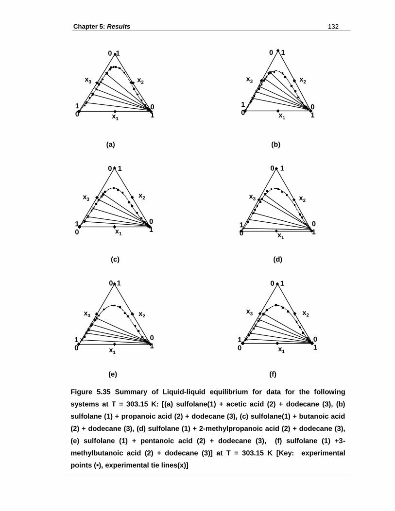
Chapter 5: Results 132
(a) (b)
(c) (d)
(e) (f)
x1
x3 x2
0 1
1 0
0 1
x3
x1
x2
0 1
1 0
0 1
x2 x3
x1
0 1
1 0
0 1
x3 x2
x1
1 0
0 1
0 1
0 1
x2 x3
x1
1 0
0 1
x2 x3
x1
0 1
1 0
0 1
Figure 5.35 Summary of Liquid-liquid equilibrium for data for the following
systems at T = 303.15 K: [(a) sulfolane(1) + acetic acid (2) + dodecane (3), (b)
sulfolane (1) + propanoic acid (2) + dodecane (3), (c) sulfolane(1) + butanoic acid
(2) + dodecane (3), (d) sulfolane (1) + 2-methylpropanoic acid (2) + dodecane (3),
(e) sulfolane (1) + pentanoic acid (2) + dodecane (3), (f) sulfolane (1) +3-
methylbutanoic acid (2) + dodecane (3)] at T = 303.15 K [Key: experimental
points (▪), experimental tie lines(x)]
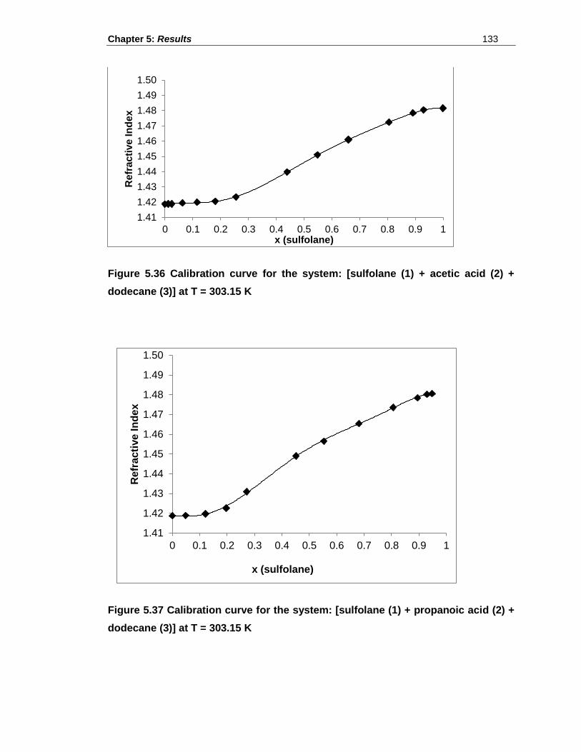
Chapter 5: Results 133
Figure 5.36 Calibration curve for the system: [sulfolane (1) + acetic acid (2) +
dodecane (3)] at T = 303.15 K
Figure 5.37 Calibration curve for the system: [sulfolane (1) + propanoic acid (2) +
dodecane (3)] at T = 303.15 K
1.41
1.42
1.43
1.44
1.45
1.46
1.47
1.48
1.49
1.50
0 0.1 0.2 0.3 0.4 0.5 0.6 0.7 0.8 0.9 1
Re
fra
cti
ve
In
de
x
x (sulfolane)
1.41
1.42
1.43
1.44
1.45
1.46
1.47
1.48
1.49
1.50
0 0.1 0.2 0.3 0.4 0.5 0.6 0.7 0.8 0.9 1
Re
fra
cti
ve
In
de
x
x (sulfolane)
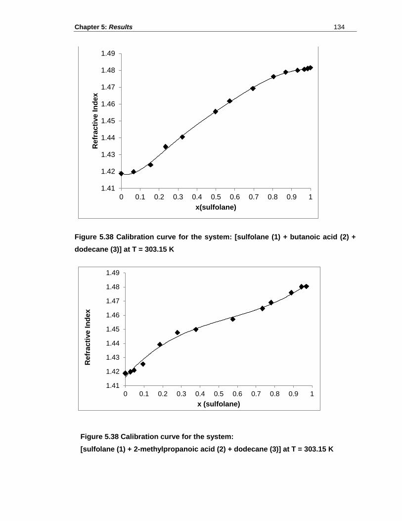
Chapter 5: Results 134
Figure 5.38 Calibration curve for the system: [sulfolane (1) + butanoic acid (2) +
dodecane (3)] at T = 303.15 K
1.41
1.42
1.43
1.44
1.45
1.46
1.47
1.48
1.49
0 0.1 0.2 0.3 0.4 0.5 0.6 0.7 0.8 0.9 1
Re
fra
cti
ve
In
de
x
x(sulfolane)
1.41
1.42
1.43
1.44
1.45
1.46
1.47
1.48
1.49
0 0.1 0.2 0.3 0.4 0.5 0.6 0.7 0.8 0.9 1
Re
fra
cti
ve
In
de
x
x (sulfolane)
Figure 5.38 Calibration curve for the system:
[sulfolane (1) + 2-methylpropanoic acid (2) + dodecane (3)] at T = 303.15 K
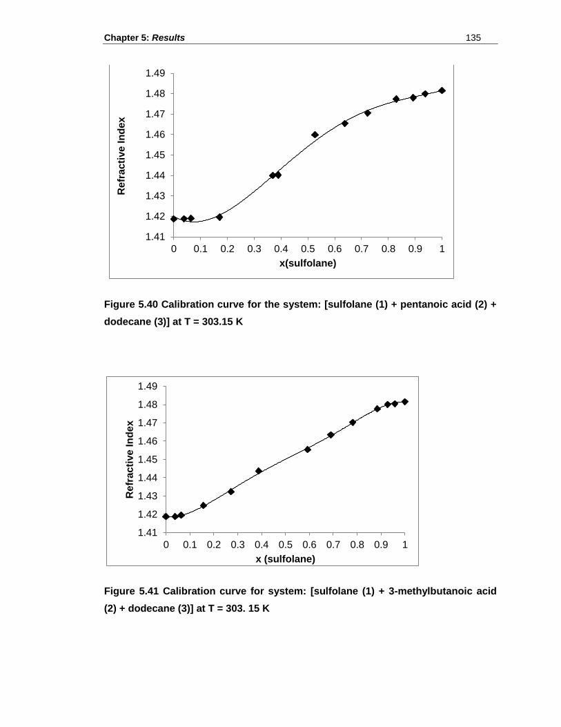
Chapter 5: Results 135
Figure 5.40 Calibration curve for the system: [sulfolane (1) + pentanoic acid (2) +
dodecane (3)] at T = 303.15 K
Figure 5.41 Calibration curve for system: [sulfolane (1) + 3-methylbutanoic acid
(2) + dodecane (3)] at T = 303. 15 K
1.41
1.42
1.43
1.44
1.45
1.46
1.47
1.48
1.49
0 0.1 0.2 0.3 0.4 0.5 0.6 0.7 0.8 0.9 1
Re
fra
cti
ve
In
de
x
x(sulfolane)
1.41
1.42
1.43
1.44
1.45
1.46
1.47
1.48
1.49
0 0.1 0.2 0.3 0.4 0.5 0.6 0.7 0.8 0.9 1
Re
fra
cti
ve
In
de
x
x (sulfolane)
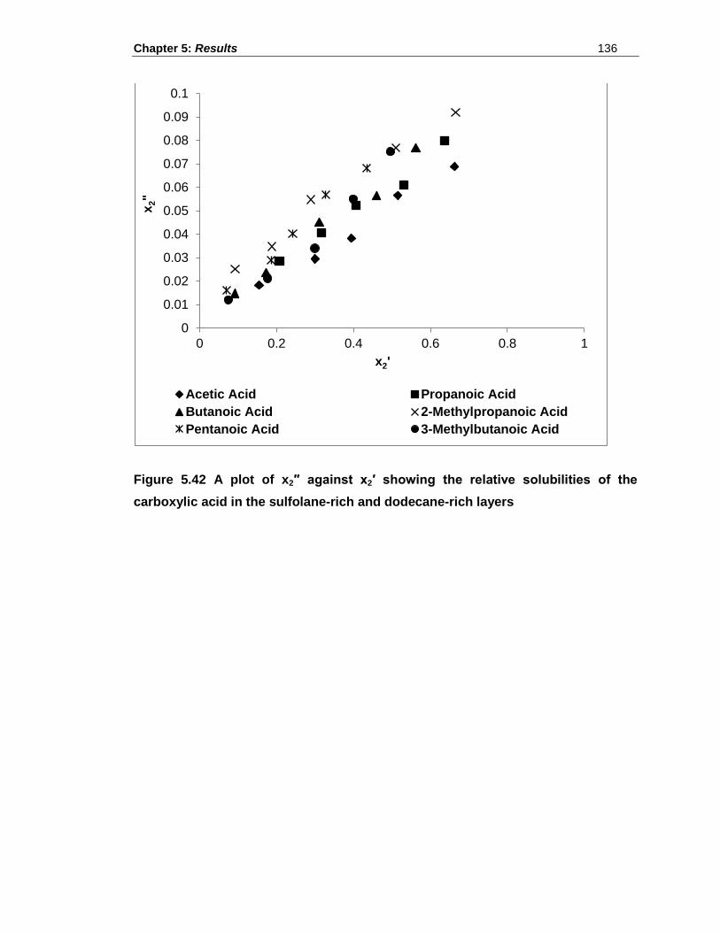
Chapter 5: Results 136
Figure 5.42 A plot of x2″ against x2′ showing the relative solubilities of the
carboxylic acid in the sulfolane-rich and dodecane-rich layers
0
0.01
0.02
0.03
0.04
0.05
0.06
0.07
0.08
0.09
0.1
0 0.2 0.4 0.6 0.8 1
x2"
x2'
Acetic Acid Propanoic Acid
Butanoic Acid 2-Methylpropanoic Acid
Pentanoic Acid 3-Methylbutanoic Acid
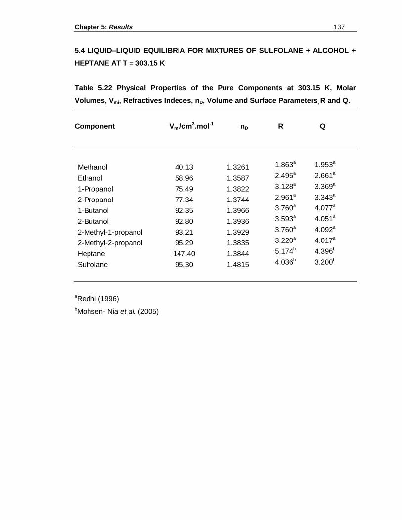
Chapter 5: Results 137
5.4 LIQUID–LIQUID EQUILIBRIA FOR MIXTURES OF SULFOLANE + ALCOHOL +
HEPTANE AT T = 303.15 K
Table 5.22 Physical Properties of the Pure Components at 303.15 K, Molar
Volumes, Vmi, Refractives Indeces, nD, Volume and Surface Parameters, R and Q.
Component Vmi/cm3.mol-1 nD R Q
Methanol 40.13 1.3261 1.863a 1.953a
Ethanol 58.96 1.3587 2.495a 2.661a
1-Propanol 75.49 1.3822 3.128a 3.369a
2-Propanol 77.34 1.3744 2.961a 3.343a
1-Butanol 92.35 1.3966 3.760a 4.077a
2-Butanol 92.80 1.3936 3.593a 4.051a
2-Methyl-1-propanol 93.21 1.3929 3.760a 4.092a
2-Methyl-2-propanol 95.29 1.3835 3.220a 4.017a
Heptane 147.40 1.3844 5.174b 4.396b
Sulfolane 95.30 1.4815 4.036b 3.200b
aRedhi (1996)
bMohsen- Nia et al. (2005)
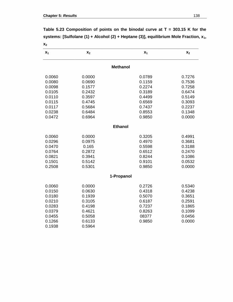
Chapter 5: Results 138
Table 5.23 Composition of points on the binodal curve at T = 303.15 K for the
systems: [Sulfolane (1) + Alcohol (2) + Heptane (3)], equilibrium Mole Fraction, x1,
x2
x1
x2
x1
x2
Methanol
0.0060
0.0000
0.0789
0.7276
0.0080
0.0690
0.1159
0.7536
0.0098
0.1577
0.2274
0.7258
0.0105
0.2432
0.3189
0.6474
0.0110
0.3597
0.4499
0.5149
0.0115
0.4745
0.6569
0.3093
0.0117
0.5684
0.7437
0.2237
0.0238
0.6484
0.8553
0.1348
0.0472
0.6964
0.9850
0.0000
Ethanol
0.0060
0.0000
0.3205
0.4991
0.0296
0.0975
0.4970
0.3681
0.0470
0.165
0.5598
0.3188
0.0764
0.2872
0.6512
0.2470
0.0821
0.3941
0.8244
0.1086
0.1501
0.5142
0.9101
0.0532
0.2508
0.5301
0.9850
0.0000
1-Propanol
0.0060
0.0000
0.2726
0.5340
0.0150
0.0630
0.4318
0.4238
0.0180
0.1939
0.5070
0.3651
0.0210
0.3105
0.6187
0.2591
0.0283
0.4198
0.7237
0.1865
0.0379
0.4621
0.8263
0.1099
0.0455
0.5058
08377
0.0456
0.1266
0.6133
0.9850
0.0000
0.1938
0.5964
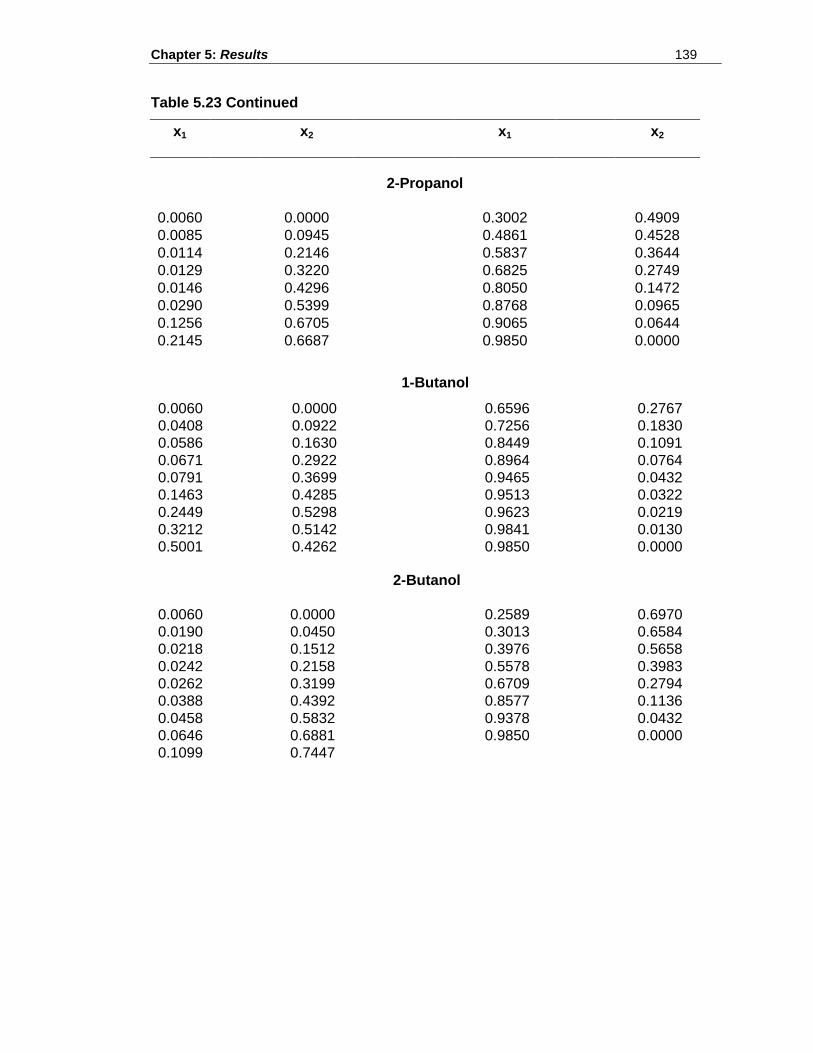
Chapter 5: Results 139
Table 5.23 Continued
x1
x2
x1
x2
2-Propanol
0.0060
0.0000
0.3002
0.4909
0.0085
0.0945
0.4861
0.4528
0.0114
0.2146
0.5837
0.3644
0.0129
0.3220
0.6825
0.2749
0.0146
0.4296
0.8050
0.1472
0.0290
0.5399
0.8768
0.0965
0.1256
0.6705
0.9065
0.0644
0.2145
0.6687
0.9850
0.0000
1-Butanol
0.0060
0.0000
0.6596
0.2767
0.0408
0.0922
0.7256
0.1830
0.0586
0.1630
0.8449
0.1091
0.0671
0.2922
0.8964
0.0764
0.0791
0.3699
0.9465
0.0432
0.1463
0.4285
0.9513
0.0322
0.2449
0.5298
0.9623
0.0219
0.3212
0.5142
0.9841
0.0130
0.5001
0.4262
0.9850
0.0000
2-Butanol
0.0060
0.0000
0.2589
0.6970
0.0190
0.0450
0.3013
0.6584
0.0218
0.1512
0.3976
0.5658
0.0242
0.2158
0.5578
0.3983
0.0262
0.3199
0.6709
0.2794
0.0388
0.4392
0.8577
0.1136
0.0458
0.5832
0.9378
0.0432
0.0646
0.6881
0.9850
0.0000
0.1099
0.7447
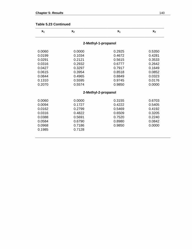
Chapter 5: Results 140
Table 5.23 Continued
x1
x2
x1
x2
2-Methyl-1-propanol
0.0060
0.0000
0.2925
0.5350
0.0199
0.1034
0.4672
0.4281
0.0291
0.2121
0.5615
0.3533
0.0316
0.2932
0.6777
0.2642
0.0427
0.3297
0.7917
0.1649
0.0615
0.3954
0.8518
0.0852
0.0844
0.4965
0.8849
0.0323
0.1310
0.5595
0.9745
0.0176
0.2070
0.5574
0.9850
0.0000
2-Methyl-2-propanol
0.0060
0.0000
0.3155
0.6703
0.0094
0.1727
0.4222
0.5405
0.0162
0.2799
0.5469
0.4192
0.0316
0.4822
0.6509
0.3205
0.0388
0.5691
0.7520
0.2240
0.0584
0.6790
0.8980
0.0842
0.0968
0.7186
0.9850
0.0000
0.1985
0.7128
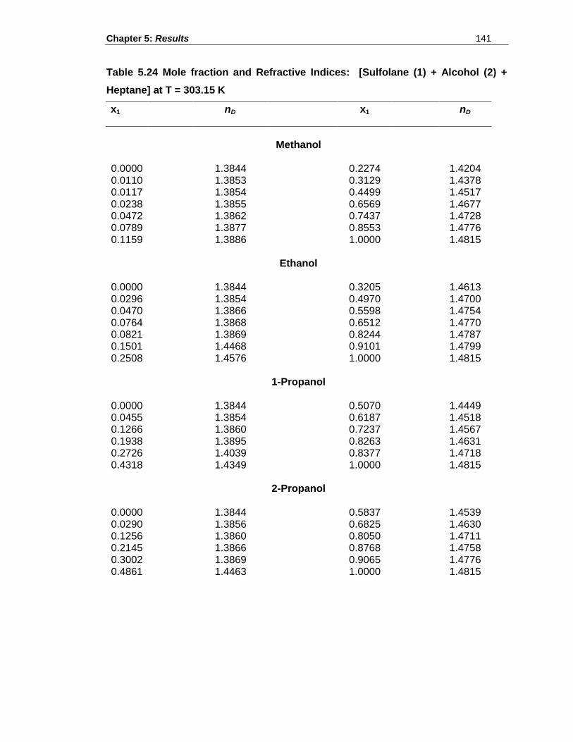
Chapter 5: Results 141
Table 5.24 Mole fraction and Refractive Indices: [Sulfolane (1) + Alcohol (2) +
Heptane] at T = 303.15 K
x1
nD
x1
nD
Methanol
0.0000
1.3844
0.2274
1.4204
0.0110
1.3853
0.3129
1.4378 0.0117
1.3854
0.4499
1.4517
0.0238
1.3855
0.6569
1.4677 0.0472
1.3862
0.7437
1.4728
0.0789
1.3877
0.8553
1.4776 0.1159
1.3886
1.0000
1.4815
Ethanol
0.0000
1.3844
0.3205
1.4613
0.0296
1.3854
0.4970
1.4700 0.0470
1.3866
0.5598
1.4754
0.0764
1.3868
0.6512
1.4770 0.0821
1.3869
0.8244
1.4787
0.1501
1.4468
0.9101
1.4799 0.2508
1.4576
1.0000
1.4815
1-Propanol
0.0000
1.3844
0.5070
1.4449
0.0455
1.3854
0.6187
1.4518 0.1266
1.3860
0.7237
1.4567
0.1938
1.3895
0.8263
1.4631 0.2726
1.4039
0.8377
1.4718
0.4318
1.4349
1.0000
1.4815
2-Propanol
0.0000
1.3844
0.5837
1.4539 0.0290
1.3856
0.6825
1.4630
0.1256
1.3860
0.8050
1.4711 0.2145
1.3866
0.8768
1.4758
0.3002
1.3869
0.9065
1.4776 0.4861
1.4463
1.0000
1.4815
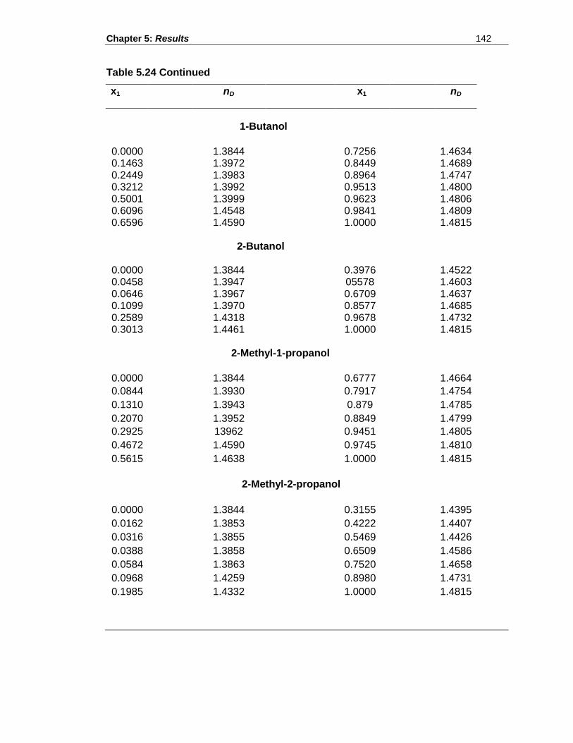
Chapter 5: Results 142
Table 5.24 Continued
x1
nD
x1
nD
1-Butanol
0.0000
1.3844
0.7256
1.4634 0.1463
1.3972
0.8449
1.4689
0.2449
1.3983
0.8964
1.4747 0.3212
1.3992
0.9513
1.4800
0.5001
1.3999
0.9623
1.4806 0.6096
1.4548
0.9841
1.4809
0.6596
1.4590
1.0000
1.4815 2-Butanol 0.0000
1.3844
0.3976
1.4522
0.0458
1.3947
05578
1.4603 0.0646
1.3967
0.6709
1.4637
0.1099
1.3970
0.8577
1.4685 0.2589
1.4318
0.9678
1.4732
0.3013
1.4461
1.0000
1.4815 2-Methyl-1-propanol
0.0000
1.3844
0.6777
1.4664
0.0844
1.3930
0.7917
1.4754
0.1310
1.3943
0.879
1.4785
0.2070
1.3952
0.8849
1.4799
0.2925
13962
0.9451
1.4805
0.4672
1.4590
0.9745
1.4810
0.5615
1.4638
1.0000
1.4815
2-Methyl-2-propanol
0.0000
1.3844
0.3155
1.4395
0.0162
1.3853
0.4222
1.4407
0.0316
1.3855
0.5469
1.4426
0.0388
1.3858
0.6509
1.4586
0.0584
1.3863
0.7520
1.4658
0.0968
1.4259
0.8980
1.4731
0.1985
1.4332
1.0000
1.4815
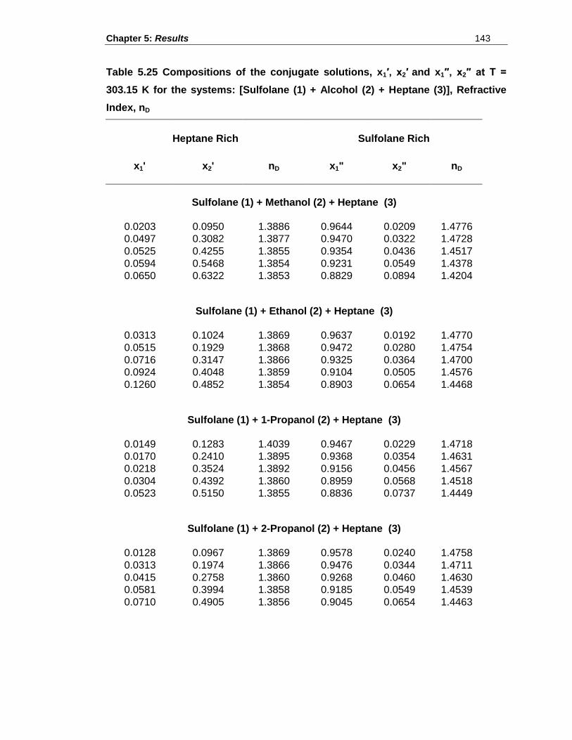
Chapter 5: Results 143
Table 5.25 Compositions of the conjugate solutions, x1′, x2′ and x1″, x2″ at T =
303.15 K for the systems: [Sulfolane (1) + Alcohol (2) + Heptane (3)], Refractive
Index, nD
Heptane Rich Sulfolane Rich
x1' x2' nD x1" x2" nD
Sulfolane (1) + Methanol (2) + Heptane (3)
0.0203 0.0950 1.3886 0.9644 0.0209 1.4776
0.0497 0.3082 1.3877 0.9470 0.0322 1.4728
0.0525 0.4255 1.3855 0.9354 0.0436 1.4517
0.0594 0.5468 1.3854 0.9231 0.0549 1.4378
0.0650 0.6322 1.3853 0.8829 0.0894 1.4204
Sulfolane (1) + Ethanol (2) + Heptane (3)
0.0313 0.1024 1.3869 0.9637 0.0192 1.4770
0.0515 0.1929 1.3868 0.9472 0.0280 1.4754
0.0716 0.3147 1.3866 0.9325 0.0364 1.4700
0.0924 0.4048 1.3859 0.9104 0.0505 1.4576
0.1260 0.4852 1.3854 0.8903 0.0654 1.4468
Sulfolane (1) + 1-Propanol (2) + Heptane (3)
0.0149 0.1283 1.4039 0.9467 0.0229 1.4718
0.0170 0.2410 1.3895 0.9368 0.0354 1.4631
0.0218 0.3524 1.3892 0.9156 0.0456 1.4567
0.0304 0.4392 1.3860 0.8959 0.0568 1.4518
0.0523 0.5150 1.3855 0.8836 0.0737 1.4449
Sulfolane (1) + 2-Propanol (2) + Heptane (3)
0.0128 0.0967 1.3869 0.9578 0.0240 1.4758
0.0313 0.1974 1.3866 0.9476 0.0344 1.4711
0.0415 0.2758 1.3860 0.9268 0.0460 1.4630
0.0581 0.3994 1.3858 0.9185 0.0549 1.4539
0.0710 0.4905 1.3856 0.9045 0.0654 1.4463
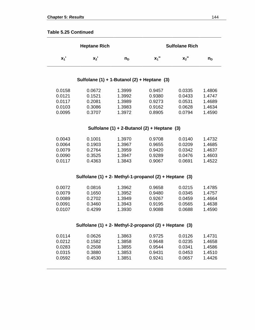
Chapter 5: Results 144
Table 5.25 Continued
Heptane Rich Sulfolane Rich
x1' x2' nD x1" x2" nD
Sulfolane (1) + 1-Butanol (2) + Heptane (3)
0.0158 0.0672 1.3999 0.9457 0.0335 1.4806
0.0121 0.1521 1.3992 0.9380 0.0433 1.4747
0.0117 0.2081 1.3989 0.9273 0.0531 1.4689
0.0103 0.3086 1.3983 0.9162 0.0628 1.4634
0.0095 0.3707 1.3972 0.8905 0.0794 1.4590
Sulfolane (1) + 2-Butanol (2) + Heptane (3)
0.0043 0.1001 1.3970 0.9708 0.0140 1.4732
0.0064 0.1903 1.3967 0.9655 0.0209 1.4685
0.0079 0.2764 1.3959 0.9420 0.0342 1.4637
0.0090 0.3525 1.3947 0.9289 0.0476 1.4603
0.0117 0.4363 1.3843 0.9067 0.0691 1.4522
Sulfolane (1) + 2- Methyl-1-propanol (2) + Heptane (3)
0.0072 0.0816 1.3962 0.9658 0.0215 1.4785
0.0079 0.1650 1.3952 0.9480 0.0345 1.4757
0.0089 0.2702 1.3949 0.9267 0.0459 1.4664
0.0091 0.3460 1.3943 0.9195 0.0565 1.4638
0.0107 0.4299 1.3930 0.9088 0.0688 1.4590
Sulfolane (1) + 2- Methyl-2-propanol (2) + Heptane (3)
0.0114 0.0626 1.3863 0.9725 0.0126 1.4731
0.0212 0.1582 1.3858 0.9648 0.0235 1.4658
0.0283 0.2508 1.3855 0.9544 0.0341 1.4586
0.0315 0.3880 1.3853 0.9431 0.0453 1.4510
0.0592 0.4530 1.3851 0.9241 0.0657 1.4426
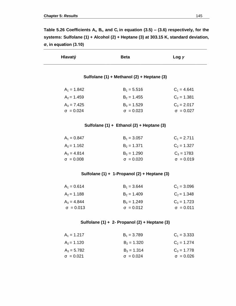
Chapter 5: Results 145
Table 5.26 Coefficients Ai, Bi, and Ci in equation (3.5) – (3.6) respectively, for the
systems: Sulfolane (1) + Alcohol (2) + Heptane (3) at 303.15 K, standard deviation,
σ, in equation (3.10)
Hlavatý
Beta
Log
Sulfolane (1) + Methanol (2) + Heptane (3)
A1 = 1.842 B1 = 5.516 C1 = 4.641
A2 = 1.459 B2 = 1.455 C2 = 1.381
A3 = 7.425 B3 = 1.529 C3 = 2.017
σ = 0.024 σ = 0.023 σ = 0.027
Sulfolane (1) + Ethanol (2) + Heptane (3)
A1 = 0.847 B1 = 3.057 C1 = 2.711
A2 = 1.162 B2 = 1.371 C2 = 1.327
A3 = 4.814 B3 = 1.290 C3 = 1783
σ = 0.008 σ = 0.020 σ = 0.019
Sulfolane (1) + 1-Propanol (2) + Heptane (3)
A1 = 0.614 B1 = 3.644 C1 = 3.096
A2 = 1.188 B2 = 1.409 C2 = 1.348
A3 = 4.844 B3 = 1.249 C3 = 1.723
σ = 0.013 σ = 0.012 σ = 0.011
Sulfolane (1) + 2- Propanol (2) + Heptane (3)
A1 = 1.217 B1 = 3.789 C1 = 3.333
A2 = 1.120 B2 = 1.320 C2 = 1.274
A3 = 5.782 B3 = 1.314 C3 = 1.778
σ = 0.021 σ = 0.024 σ = 0.026
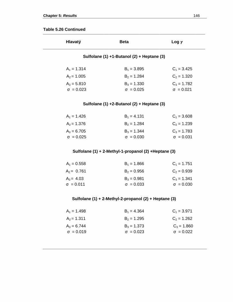
Chapter 5: Results 146
Table 5.26 Continued
Hlavatý
Beta
Log
Sulfolane (1) +1-Butanol (2) + Heptane (3)
A1 = 1.314 B1 = 3.895 C1 = 3.425
A2 = 1.005 B2 = 1.284 C2 = 1.320
A3 = 5.810 B3 = 1.330 C3 = 1.782
σ = 0.023 σ = 0.025 σ = 0.021
Sulfolane (1) +2-Butanol (2) + Heptane (3)
A1 = 1.426 B1 = 4.131 C1 = 3.608
A2 = 1.376 B2 = 1.284 C2 = 1.239
A3 = 6.705 B3 = 1.344 C3 = 1.783
σ = 0.025 σ = 0.030 σ = 0.031
Sulfolane (1) + 2-Methyl-1-propanol (2) +Heptane (3)
A1 = 0.558 B1 = 1.866 C1 = 1.751
A2 = 0.761 B2 = 0.956 C2 = 0.939
A3 = 4.03 B3 = 0.981 C3 = 1.341
σ = 0.011 σ = 0.033 σ = 0.030
Sulfolane (1) + 2-Methyl-2-propanol (2) + Heptane (3)
A1 = 1.498 B1 = 4.364 C1 = 3.971
A2 = 1.311 B2 = 1.295 C2 = 1.262
A3 = 6.744 B3 = 1.373 C3 = 1.860
σ = 0.019 σ = 0.023 σ = 0.022
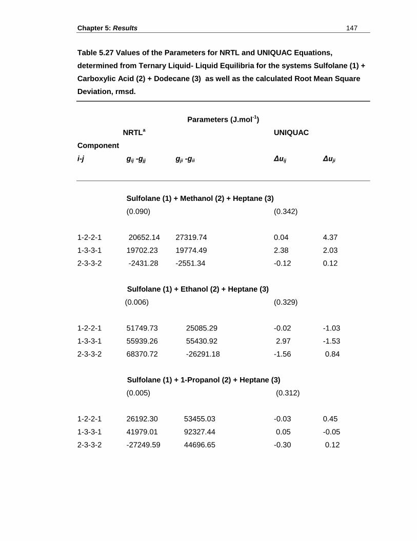
Chapter 5: Results 147
Table 5.27 Values of the Parameters for NRTL and UNIQUAC Equations,
determined from Ternary Liquid- Liquid Equilibria for the systems Sulfolane (1) +
Carboxylic Acid (2) + Dodecane (3) as well as the calculated Root Mean Square
Deviation, rmsd.
Parameters (J.mol-1)
NRTLa UNIQUAC
Component
i-j gij -gjj gji -gii Δuij Δuji
Sulfolane (1) + Methanol (2) + Heptane (3)
(0.090) (0.342)
1-2-2-1 20652.14 27319.74 0.04 4.37
1-3-3-1 19702.23 19774.49 2.38 2.03
2-3-3-2 -2431.28 -2551.34 -0.12 0.12
Sulfolane (1) + Ethanol (2) + Heptane (3)
(0.006) (0.329)
1-2-2-1 51749.73 25085.29 -0.02 -1.03
1-3-3-1 55939.26 55430.92 2.97 -1.53
2-3-3-2 68370.72 -26291.18 -1.56 0.84
Sulfolane (1) + 1-Propanol (2) + Heptane (3)
(0.005) (0.312)
1-2-2-1 26192.30 53455.03 -0.03 0.45
1-3-3-1 41979.01 92327.44 0.05 -0.05
2-3-3-2 -27249.59 44696.65 -0.30 0.12
Chapter 5: Results 148
Table 5.27 Continued
Parameters (J.mol-1)
NRTLa UNIQUAC
Component
i-j gij -gjj gji -gii Δuij Δuji
Sulfolane (1) + 2-Propanol (2) + Heptane (3)
(0.103) (0.319)
1-2-2-1 11914.00 25083.08 0.65 0.77
1-3-3-1 18737.89 22867.93 0.006 -0.02
2-3-3-2 4937.57 -18661.94 -0.29 0.09
Sulfolane (1) + 1-Butanol (2) + Heptane (3)
(0.004) (0.213)
1-2-2-1 16147.69 126181.15 -0.17 -0.50
1-3-3-1 56327.12 78031.74 0.64 0.96
2-3-3-2 37089.90 6351.67 0.11 0.64
Sulfolane (1) + 2-Butanol (2) + Heptane (3)
(0.004) (0.337)
1-2-2-1 16593.96 35691.37 0.41 -0.31
1-3-3-1 62280.03 217070.41 0.43 0.55
2-3-3-2 42946.12 -50825.51 0.34 0.86
Chapter 5: Results 149
Table 5.27 Continued
Parameters (J.mol-1)
NRTLa UNIQUAC
Component
i-j gij -gjj gji -gii Δuij Δuji
Sulfolane (1) + 2-Methyl-1-propanol (2) + Heptane (3)
(0.003) (0.336)
1-2-2-1 33957.98 39328.79 0.53 -0.17
1-3-3-1 57924.81 16408.25 -0.01 -0.07
2-3-3-2 2846.29 21180.06 0.21 0.23
Sulfolane (1) + 2-Methyl-2-propanol (2) + Heptane (3)
(0.002) (0.353)
1-2-2-1 43371.93 24834.39 0.38 0.68
1-3-3-1 71078.28 81110.37 0.61 -0.66
2-3-3-2 -5704.28 20830.61 -0.83 0.92
aCalculated with αij =0.2
Chapter 5: Results 150
Table 5.28 Representative selectivity values of sulfolane for the separation of
alcohol from heptane using equation (3.1)
Alcohol Selectivity (ω)
Methanol 5
Ethanol 8
1-Propanol 3
2-Propanol 6
1-Butanol 11
2-Butanol 5
2-Methyl-1-propanol 8
2-Methyl-2-propanol 9
Chapter 5: Results 151
Figure 5.43 Liquid-liquid equilibrium data for the system [sulfolane (1) + methanol
(2) + heptane (3)] at T = 303.15 K
Figure 5.43 Liquid-liquid equilibrium data for the system [sulfolane (1) + ethanol
(2) + heptane (3)] at T = 303.15 K
x2 x3
x1
0 1
0 1
1 0
x1
0 1
1
0 1
x2 x3
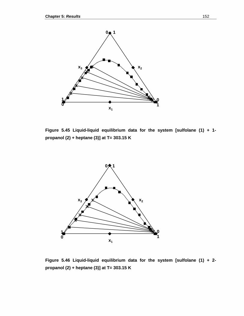
Chapter 5: Results 152
Figure 5.45 Liquid-liquid equilibrium data for the system [sulfolane (1) + 1-
propanol (2) + heptane (3)] at T= 303.15 K
Figure 5.46 Liquid-liquid equilibrium data for the system [sulfolane (1) + 2-
propanol (2) + heptane (3)] at T= 303.15 K
x2 x3
x1
0 1
0 1
1 0
x2 x3
x1
0 1
1 0
0 1
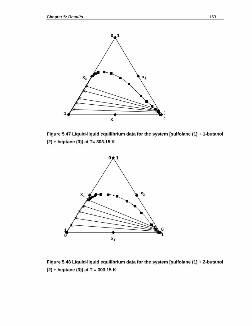
Chapter 5: Results 153
Figure 5.47 Liquid-liquid equilibrium data for the system [sulfolane (1) + 1-butanol
(2) + heptane (3)] at T= 303.15 K
Figure 5.48 Liquid-liquid equilibrium data for the system [sulfolane (1) + 2-butanol
(2) + heptane (3)] at T = 303.15 K
x3 x2
x1
1 0
1
0 1
x3 x2
1 0
0 1
0 1
x1
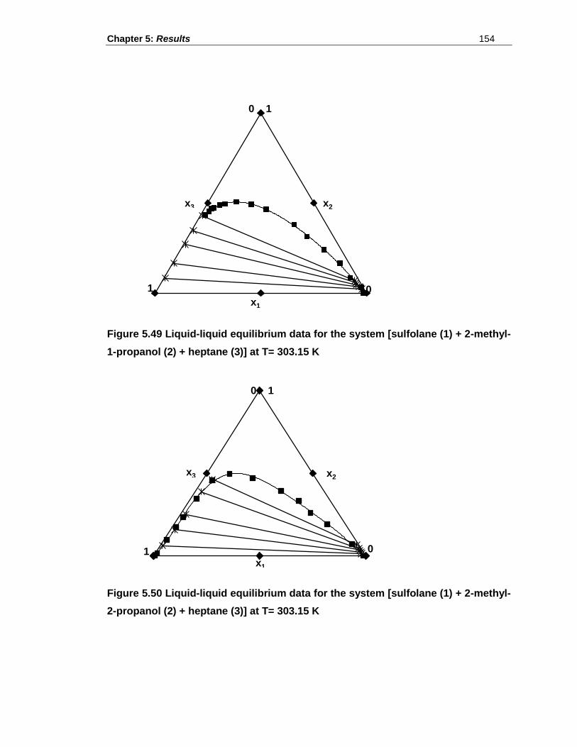
Chapter 5: Results 154
Figure 5.49 Liquid-liquid equilibrium data for the system [sulfolane (1) + 2-methyl-
1-propanol (2) + heptane (3)] at T= 303.15 K
Figure 5.50 Liquid-liquid equilibrium data for the system [sulfolane (1) + 2-methyl-
2-propanol (2) + heptane (3)] at T= 303.15 K
1 0
0 1
x3 x2
x1
1 0
0 1
x2
x1
x3
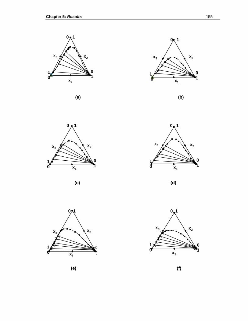
Chapter 5: Results 155
(a) (b)
(c) (d)
(e) (f)
x2 x3
x1
0 1
0 1
1 0
x1
0 1
1 0
0 1
x2 x3
x2 x3
x1
0 1
0 1
1 0
x2 x3
x1
0 1
1 0
0 1
x3 x2
x1
1
0 0
1
0 1
x3 x2
1 0
0 1
0 1
x1
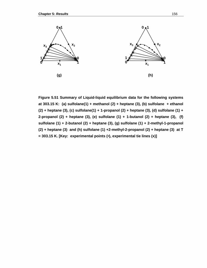
Chapter 5: Results 156
(g) (h)
Figure 5.51 Summary of Liquid-liquid equilibrium data for the following systems
at 303.15 K: (a) sulfolane(1) + methanol (2) + heptane (3), (b) sulfolane + ethanol
(2) + heptane (3), (c) sulfolane(1) + 1-propanol (2) + heptane (3), (d) sulfolane (1) +
2-propanol (2) + heptane (3), (e) sulfolane (1) + 1-butanol (2) + heptane (3), (f)
sulfolane (1) + 2-butanol (2) + heptane (3), (g) sulfolane (1) + 2-methyl-1-propanol
(2) + heptane (3) and (h) sulfolane (1) +2-methyl-2-propanol (2) + heptane (3) at T
= 303.15 K. [Key: experimental points (▪), experimental tie lines (x)]
1 0
0 1
0 1
x3 x2
x1
1 0
0 1
0 1
x2
x1
x3
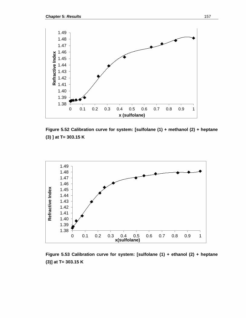
Chapter 5: Results 157
Figure 5.52 Calibration curve for system: [sulfolane (1) + methanol (2) + heptane
(3) ] at T= 303.15 K
Figure 5.53 Calibration curve for system: [sulfolane (1) + ethanol (2) + heptane
(3)] at T= 303.15 K
1.38
1.39
1.40
1.41
1.42
1.43
1.44
1.45
1.46
1.47
1.48
1.49
0 0.1 0.2 0.3 0.4 0.5 0.6 0.7 0.8 0.9 1
Re
fra
cti
ve
In
de
x
x (sulfolane)
1.38
1.39
1.40
1.41
1.42
1.43
1.44
1.45
1.46
1.47
1.48
1.49
0 0.1 0.2 0.3 0.4 0.5 0.6 0.7 0.8 0.9 1
Re
fra
cti
ve
In
de
x
x(sulfolane)
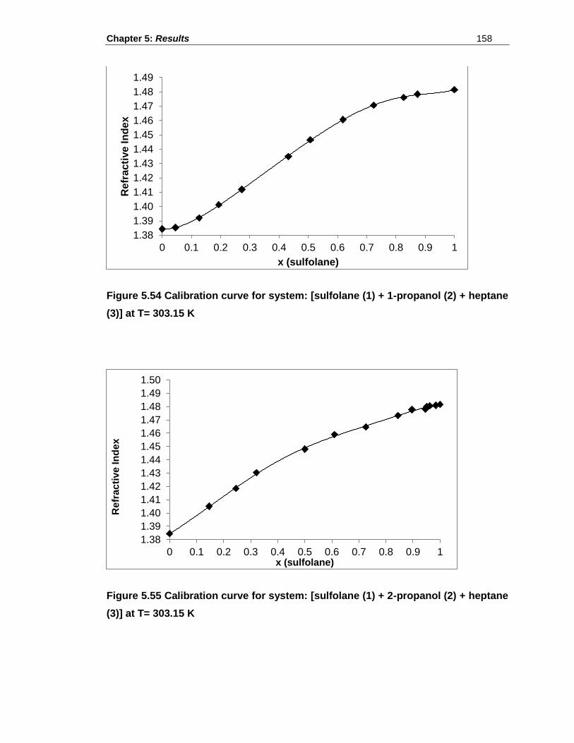
Chapter 5: Results 158
Figure 5.54 Calibration curve for system: [sulfolane (1) + 1-propanol (2) + heptane
(3)] at T= 303.15 K
Figure 5.55 Calibration curve for system: [sulfolane (1) + 2-propanol (2) + heptane
(3)] at T= 303.15 K
1.38
1.39
1.40
1.41
1.42
1.43
1.44
1.45
1.46
1.47
1.48
1.49
0 0.1 0.2 0.3 0.4 0.5 0.6 0.7 0.8 0.9 1
Re
fra
cti
ve
In
de
x
x (sulfolane)
1.38
1.39
1.40
1.41
1.42
1.43
1.44
1.45
1.46
1.47
1.48
1.49
1.50
0 0.1 0.2 0.3 0.4 0.5 0.6 0.7 0.8 0.9 1
Re
fra
cti
ve
In
de
x
x (sulfolane)
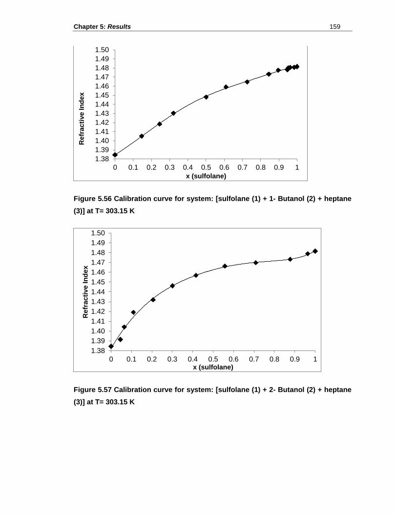
Chapter 5: Results 159
Figure 5.56 Calibration curve for system: [sulfolane (1) + 1- Butanol (2) + heptane
(3)] at T= 303.15 K
Figure 5.57 Calibration curve for system: [sulfolane (1) + 2- Butanol (2) + heptane
(3)] at T= 303.15 K
1.38
1.39
1.40
1.41
1.42
1.43
1.44
1.45
1.46
1.47
1.48
1.49
1.50
0 0.1 0.2 0.3 0.4 0.5 0.6 0.7 0.8 0.9 1
Re
fra
cti
ve
In
de
x
x (sulfolane)
1.38
1.39
1.40
1.41
1.42
1.43
1.44
1.45
1.46
1.47
1.48
1.49
1.50
0 0.1 0.2 0.3 0.4 0.5 0.6 0.7 0.8 0.9 1
Re
fra
cti
ve
In
de
x
x (sulfolane)
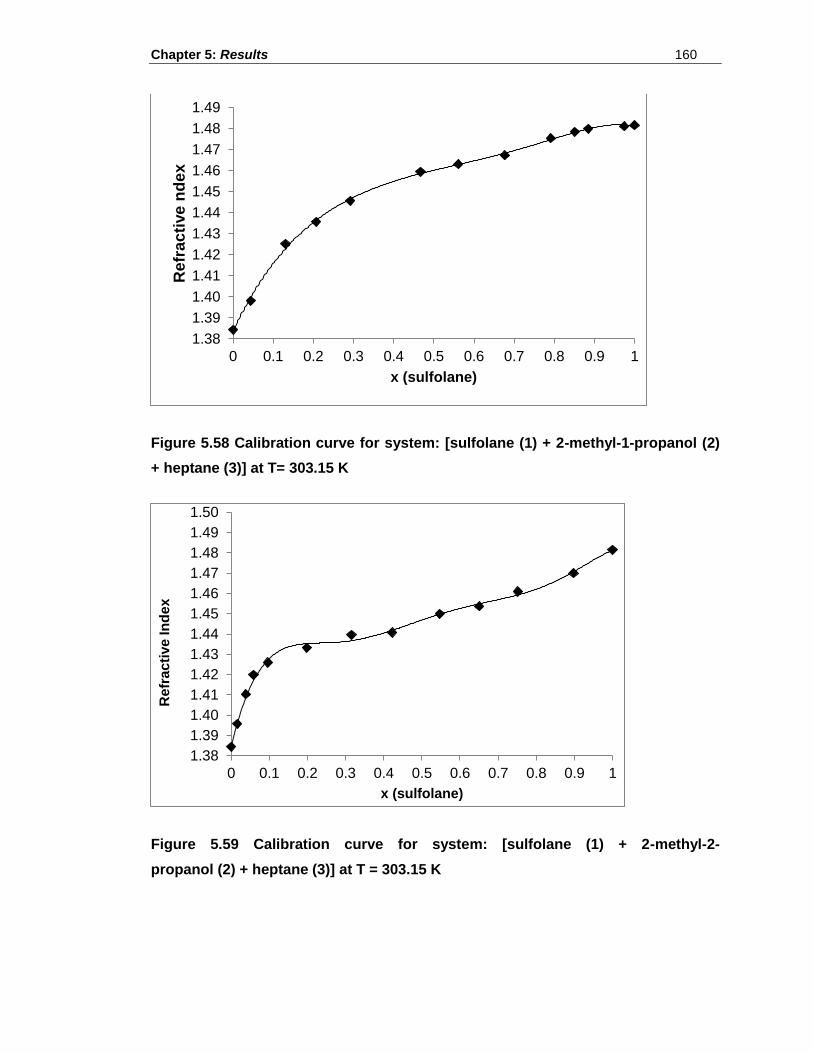
Chapter 5: Results 160
Figure 5.58 Calibration curve for system: [sulfolane (1) + 2-methyl-1-propanol (2)
+ heptane (3)] at T= 303.15 K
Figure 5.59 Calibration curve for system: [sulfolane (1) + 2-methyl-2-
propanol (2) + heptane (3)] at T = 303.15 K
1.38
1.39
1.40
1.41
1.42
1.43
1.44
1.45
1.46
1.47
1.48
1.49
0 0.1 0.2 0.3 0.4 0.5 0.6 0.7 0.8 0.9 1
Refr
ac
tive
nd
ex
x (sulfolane)
1.38
1.39
1.40
1.41
1.42
1.43
1.44
1.45
1.46
1.47
1.48
1.49
1.50
0 0.1 0.2 0.3 0.4 0.5 0.6 0.7 0.8 0.9 1
Re
fra
cti
ve
In
de
x
x (sulfolane)
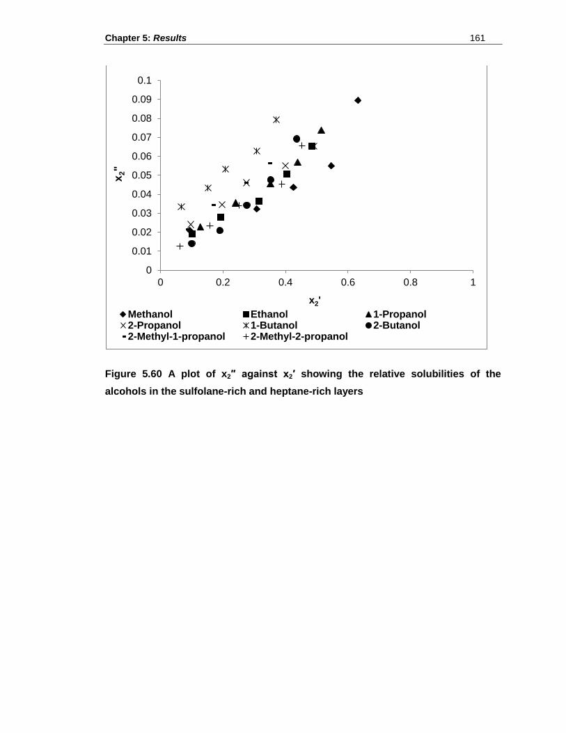
Chapter 5: Results 161
Figure 5.60 A plot of x2″ against x2′ showing the relative solubilities of the
alcohols in the sulfolane-rich and heptane-rich layers
0
0.01
0.02
0.03
0.04
0.05
0.06
0.07
0.08
0.09
0.1
0 0.2 0.4 0.6 0.8 1
x2"
x2'
Methanol Ethanol 1-Propanol2-Propanol 1-Butanol 2-Butanol2-Methyl-1-propanol 2-Methyl-2-propanol
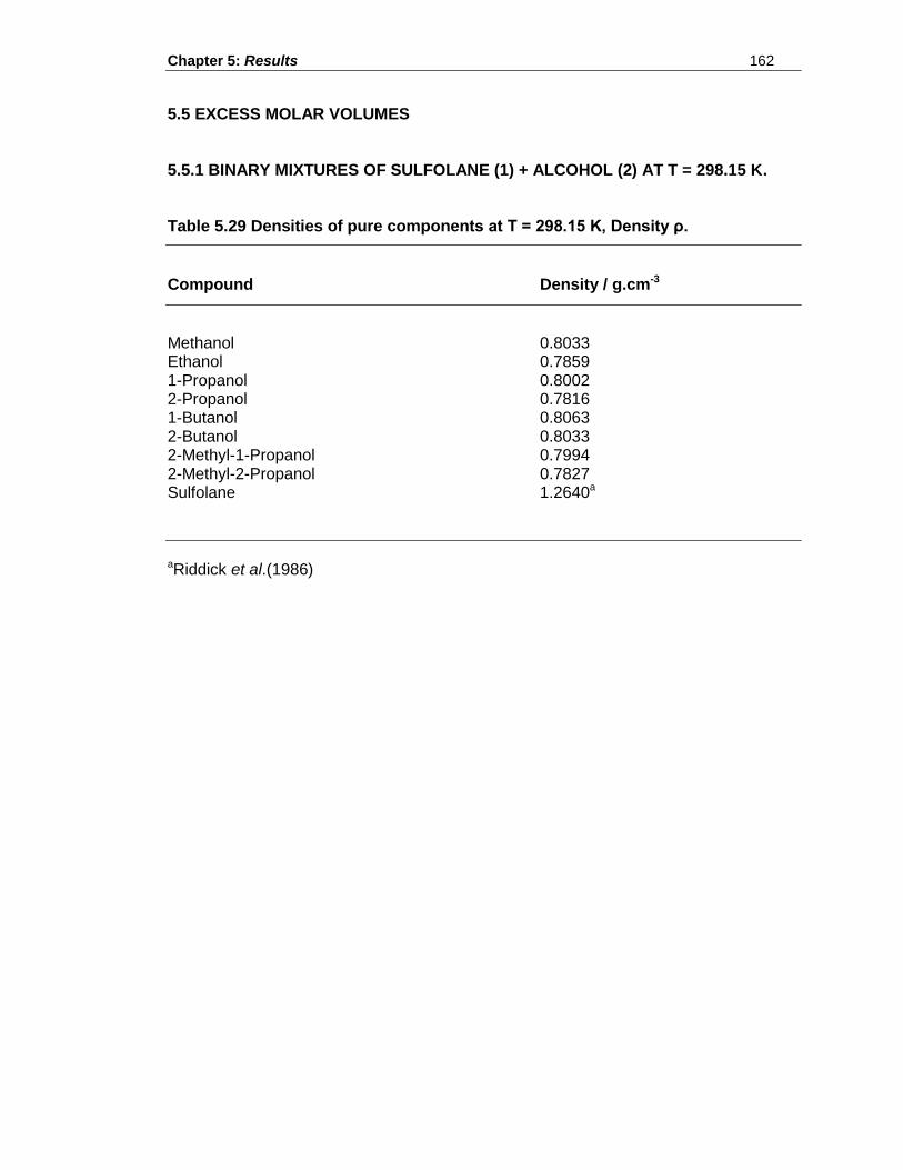
Chapter 5: Results 162
5.5 EXCESS MOLAR VOLUMES
5.5.1 BINARY MIXTURES OF SULFOLANE (1) + ALCOHOL (2) AT T = 298.15 K.
Table 5.29 Densities of pure components at T = 298.15 K, Density ρ.
Compound Density / g.cm-3
Methanol 0.8033 Ethanol 0.7859 1-Propanol 0.8002 2-Propanol 0.7816 1-Butanol 0.8063 2-Butanol 0.8033 2-Methyl-1-Propanol 0.7994 2-Methyl-2-Propanol 0.7827 Sulfolane 1.2640a
aRiddick et al.(1986)
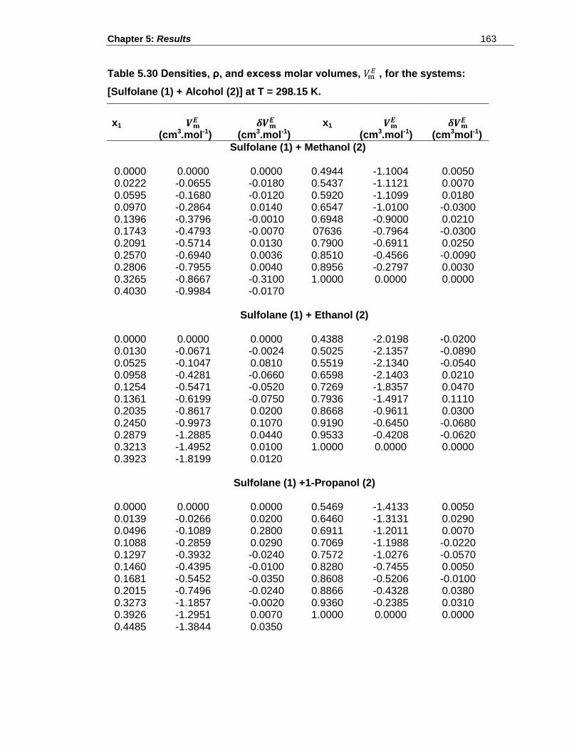
Chapter 5: Results 163
Table 5.30 Densities, ρ, and excess molar volumes, , for the systems:
[Sulfolane (1) + Alcohol (2)] at T = 298.15 K.
x1
x1
(cm3.mol-1) (cm3.mol-1)
(cm3.mol-1) (cm3mol-1) Sulfolane (1) + Methanol (2)
0.0000 0.0000 0.0000 0.4944 -1.1004 0.0050 0.0222 -0.0655 -0.0180 0.5437 -1.1121 0.0070 0.0595 -0.1680 -0.0120 0.5920 -1.1099 0.0180 0.0970 -0.2864 0.0140 0.6547 -1.0100 -0.0300 0.1396 -0.3796 -0.0010 0.6948 -0.9000 0.0210 0.1743 -0.4793 -0.0070 07636 -0.7964 -0.0300 0.2091 -0.5714 0.0130 0.7900 -0.6911 0.0250 0.2570 -0.6940 0.0036 0.8510 -0.4566 -0.0090 0.2806 -0.7955 0.0040 0.8956 -0.2797 0.0030 0.3265 -0.8667 -0.3100 1.0000 0.0000 0.0000 0.4030 -0.9984 -0.0170
Sulfolane (1) + Ethanol (2)
0.0000 0.0000 0.0000 0.4388 -2.0198 -0.0200
0.0130 -0.0671 -0.0024 0.5025 -2.1357 -0.0890 0.0525 -0.1047 0.0810 0.5519 -2.1340 -0.0540 0.0958 -0.4281 -0.0660 0.6598 -2.1403 0.0210 0.1254 -0.5471 -0.0520 0.7269 -1.8357 0.0470 0.1361 -0.6199 -0.0750 0.7936 -1.4917 0.1110 0.2035 -0.8617 0.0200 0.8668 -0.9611 0.0300 0.2450 -0.9973 0.1070 0.9190 -0.6450 -0.0680 0.2879 -1.2885 0.0440 0.9533 -0.4208 -0.0620 0.3213 -1.4952 0.0100 1.0000 0.0000 0.0000 0.3923 -1.8199 0.0120
Sulfolane (1) +1-Propanol (2)
0.0000 0.0000 0.0000 0.5469 -1.4133 0.0050
0.0139 -0.0266 0.0200 0.6460 -1.3131 0.0290 0.0496 -0.1089 0.2800 0.6911 -1.2011 0.0070 0.1088 -0.2859 0.0290 0.7069 -1.1988 -0.0220 0.1297 -0.3932 -0.0240 0.7572 -1.0276 -0.0570 0.1460 -0.4395 -0.0100 0.8280 -0.7455 0.0050 0.1681 -0.5452 -0.0350 0.8608 -0.5206 -0.0100 0.2015 -0.7496 -0.0240 0.8866 -0.4328 0.0380 0.3273 -1.1857 -0.0020 0.9360 -0.2385 0.0310 0.3926 -1.2951 0.0070 1.0000 0.0000 0.0000 0.4485 -1.3844 0.0350
Chapter 5: Results 164
Table 5.30 Continued
x1
x1
(cm3.mol-1) (cm3.mol-1)
(cm3.mol-1) (cm3mol-1)
Sulfolane (1) + 2-Propanol (2) 0.0000 0.0000 0.0000 0.5147 -2.0399 -0.0500
0.0535 -0.1908 0.0200 0.5747 -2.0418 -0.4700 0.0832 -0.3214 0.0160 0.6100 -2.0552 -0.5500 0.1252 -0.5421 -0.0160 0.6283 -1.9995 0.0200 0.1833 -0.8364 -0.0320 0.7240 -1.7419 0.1920 0.2333 -1.0385 0.0120 0.7529 -1.5889 -0.0880 0.2586 -1.1617 0.0120 0.8029 -1.2384 -0.0280 0.2759 -1.2741 -0.0170 0.8787 -0.6907 0.0220 0.3564 -1.5891 0.0270 0.9190 -0.4227 0.0240 0.3824 -1.6865 0.0310 1.0000 0.0000 0.0000 0.4652 -1.9828 0.0020
Sulfolane (1) + 1-Butanol (2)
0.0000 0.0000 0.0000 0.5890 -1.1425 -0.0170 0.0258 -0.0868 0.0320 0.6590 -1.1218 -0.0220 0.1021 -0.2966 -0.0060 0.6859 -1.0592 0.1070 0.1257 -0.3620 0.0025 0.7124 -0.9880 -0.0500 0.1642 -0.5444 0.0080 0.7641 -0.8479 -0.0590 0.2494 -0.7379 -0.0510 0.8118 -0.6878 -0.0510 0.3141 -0.9589 -0.0280 0.8357 -0.5924 0.0260 0.3428 -1.0196 -0.0050 0.8790 -0.4313 0.0760 0.3965 -1.1283 0.0340 0.9277 -0.2141 0.00023 0.4558 -1.1800 0.0180 1.0000 0.0000 0.0000 0.5133 -1.1673 0.0020
Sulfolane (1) + 2-Butanol (2)
0.0000 0.0000 0.0000 0.5502 -1.2181 0.0120 0.0489 -0.0944 0.0090 0.5942 -1.1921 0.0160 0.1106 -0.3207 0.0340 0.6618 -1.1299 0.0080 0.1640 -0.5124 0.0160 0.6852 -1.1022 -0.0150 0.1965 -0.6707 0.0010 0.7243 -1.0178 -0.0140 0.2502 -0.8283 -0.0460 0.8053 -0.7655 -0.0530 0.3153 -0.9905 -0.3200 0.8543 -0.5437 0.0220 0.3459 -1.0541 -0.0250 0.8979 -0.3278 -0.0130 0.4025 -1.1521 0.0210 0.9384 -0.2103 0.0770 0.4524 -1.1925 0.0390 1.0000 0.0000 0.0000 0.5052 -1.2092 0.0140
Chapter 5: Results 165
Table 5.30 Continued
x1
x1
(cm3.mol-1) (cm3.mol-1)
(cm3.mol-1) (cm3mol-1)
Sulfolane (1) + 2- Methyl-1-propanol (2)
0.0000 0.0000 0.0000 0.6161 -1.1200 -0.0072
0.0599 -0.1290 0.0510 0.6571 -1.0928 -0.0043
0.0716 -0.1921 0.0020 0.7167 -1.0050 -0.029
0.1949 -0.2731 0.0120 0.7324 -0.9062 -0.0300
0.2394 -0.5705 -0.1400 0.7935 -0.7655 -0.0210
0.2830 -0.8171 -0.0500 0.8533 -0.4919 0.0530
0.3487 -0.9951 -0.1400 0.8933 -0.3262 0.0140
0.3986 -1.0024 0.0130 0.9289 -0.1204 -0.0320
0.4444 -1.1021 0.0110 0.9533 -0.0281 0.0300
0.4965 -1.1621 0.0230 1.0000 0.0000 0.0000
0.5513 -1.1937 0.0200
Sulfolane (1) + 2-Methyl-2-propanol (2)
0.0000 0.0000 0.0000 0.4563 -1.2325 -0.0340
0.0136 -0.0290 -0.0970 0.5217 -1.2451 0.0650
0.0591 -0.1485 -0.0700 0.6263 -1.2367 0.0070
0.0835 -0.2248 0.1060 0.7114 -1.1168 -0.0270
0.1054 -0.3484 0.0070 0.7523 -0.9833 0.0460
0.1285 -0.4234 0.0230 0.7815 -0.8765 -0.0040
0.1540 -0.5306 0.0230 0.8470 -0.5433 0.0250
0.1935 -0.6412 -0.0050 0.9289 -0.2156 -0.0670
0.2191 -0.7948 -0.1100 0.9533 -0.1481 0.0060
0.2836 -1.0099 -0.0340 1.0000 0.0000 0.0000
0.3441 -1.1297 -0.0380
Chapter 5: Results 166
Table 5.31 Coefficients, Ar and standard deviations from equation for the excess
molar volumes of systems [Sulfolane (1) + Alcohol (2)] at T = 298.15 K.
Alcohol
A0 A1 A2 A3 σ
T = 298.15 K
Methanol -4.509 0.584 3.117 -2.909 0.020 Ethanol -8.573 3.003 6.024 -3.740 0.064 1-Propanol -2.477 0.959 0.531 -0.132 0.028 2-Propanol -8.092 2.654 4.120 -2.418 0.059 1-Butanol -4.645 1.343 2.936 -0.720 0.045 2-Butanol -2.791 3.309 0.894 -2.816 0.032 2-Methyl-1-propanol -5.302 -2.449 5.392 4.058 0.050 2-Methyl-2-propanol -4.175 3.056 3.420 -3.805 0.029
Chapter 5: Results 167
Figure 5.61 Plot of excess molar volume, , for binary mixtures of [sulfolane(1)
+ methanol (2)], [sulfolane (1) + ethanol (2)], [sulfolane (1) + 1-propanol (2)],
[sulfolane (1) + 2-propanol (2)], [sulfolane (1) + 1-butanol (2)], [sulfolane (1) + 2-
butanol (2)], [sulfolane (1) + 2-methyl-1-propanol (2)], [sulfolane (1) +2-methyl-2-
propanol (2)] at T = 298.15 K, as a function of mole fraction of x (sulfolane)
-2.5
-2
-1.5
-1
-0.5
0
0 0.1 0.2 0.3 0.4 0.5 0.6 0.7 0.8 0.9 1V
Em
(c
m3.m
ol-
1)
x (sulfolane)
Methanol Ethanol 1-Propanol
2-Propanol 1-Butanol 2-Butanol
2-Methyl-1-propanol 2-Methyl-2-propanol
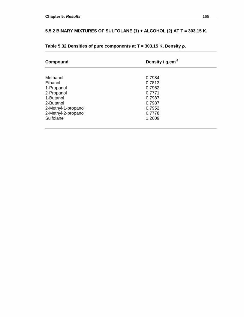
Chapter 5: Results 168
5.5.2 BINARY MIXTURES OF SULFOLANE (1) + ALCOHOL (2) AT T = 303.15 K.
Table 5.32 Densities of pure components at T = 303.15 K, Density ρ.
Compound Density / g.cm-3
Methanol 0.7984 Ethanol 0.7813 1-Propanol 0.7962 2-Propanol 0.7771 1-Butanol 0.7987 2-Butanol 0.7987 2-Methyl-1-propanol 0.7952 2-Methyl-2-propanol 0.7778 Sulfolane 1.2609
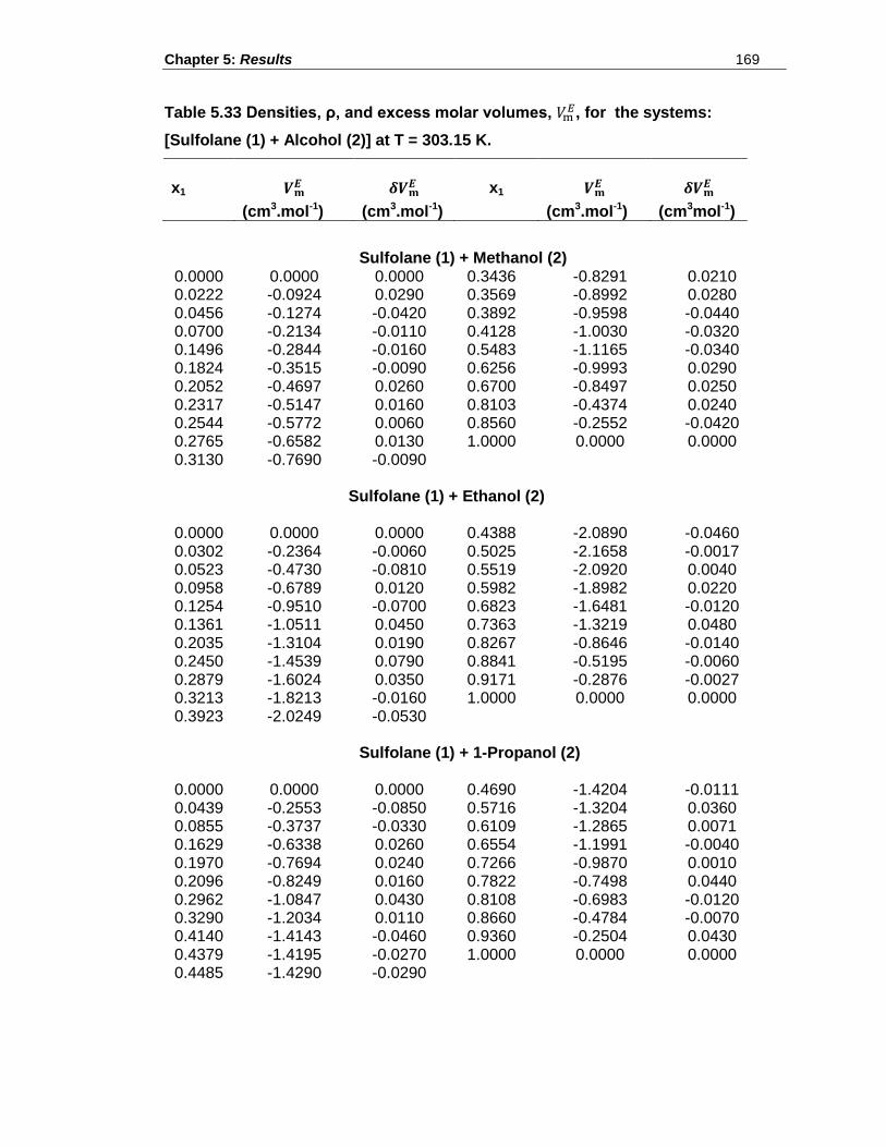
Chapter 5: Results 169
Table 5.33 Densities, ρ, and excess molar volumes, , for the systems:
[Sulfolane (1) + Alcohol (2)] at T = 303.15 K.
x1
x1
(cm3.mol-1) (cm3.mol-1)
(cm3.mol-1) (cm3mol-1)
Sulfolane (1) + Methanol (2) 0.0000 0.0000 0.0000 0.3436 -0.8291 0.0210 0.0222 -0.0924 0.0290 0.3569 -0.8992 0.0280 0.0456 -0.1274 -0.0420 0.3892 -0.9598 -0.0440 0.0700 -0.2134 -0.0110 0.4128 -1.0030 -0.0320 0.1496 -0.2844 -0.0160 0.5483 -1.1165 -0.0340 0.1824 -0.3515 -0.0090 0.6256 -0.9993 0.0290 0.2052 -0.4697 0.0260 0.6700 -0.8497 0.0250 0.2317 -0.5147 0.0160 0.8103 -0.4374 0.0240 0.2544 -0.5772 0.0060 0.8560 -0.2552 -0.0420 0.2765 -0.6582 0.0130 1.0000 0.0000 0.0000 0.3130 -0.7690 -0.0090
Sulfolane (1) + Ethanol (2) 0.0000 0.0000 0.0000 0.4388 -2.0890 -0.0460 0.0302 -0.2364 -0.0060 0.5025 -2.1658 -0.0017 0.0523 -0.4730 -0.0810 0.5519 -2.0920 0.0040 0.0958 -0.6789 0.0120 0.5982 -1.8982 0.0220 0.1254 -0.9510 -0.0700 0.6823 -1.6481 -0.0120 0.1361 -1.0511 0.0450 0.7363 -1.3219 0.0480 0.2035 -1.3104 0.0190 0.8267 -0.8646 -0.0140 0.2450 -1.4539 0.0790 0.8841 -0.5195 -0.0060 0.2879 -1.6024 0.0350 0.9171 -0.2876 -0.0027 0.3213 -1.8213 -0.0160 1.0000 0.0000 0.0000 0.3923 -2.0249 -0.0530
Sulfolane (1) + 1-Propanol (2)
0.0000 0.0000 0.0000 0.4690 -1.4204 -0.0111 0.0439 -0.2553 -0.0850 0.5716 -1.3204 0.0360 0.0855 -0.3737 -0.0330 0.6109 -1.2865 0.0071 0.1629 -0.6338 0.0260 0.6554 -1.1991 -0.0040 0.1970 -0.7694 0.0240 0.7266 -0.9870 0.0010 0.2096 -0.8249 0.0160 0.7822 -0.7498 0.0440 0.2962 -1.0847 0.0430 0.8108 -0.6983 -0.0120 0.3290 -1.2034 0.0110 0.8660 -0.4784 -0.0070 0.4140 -1.4143 -0.0460 0.9360 -0.2504 0.0430 0.4379 -1.4195 -0.0270 1.0000 0.0000 0.0000 0.4485 -1.4290 -0.0290
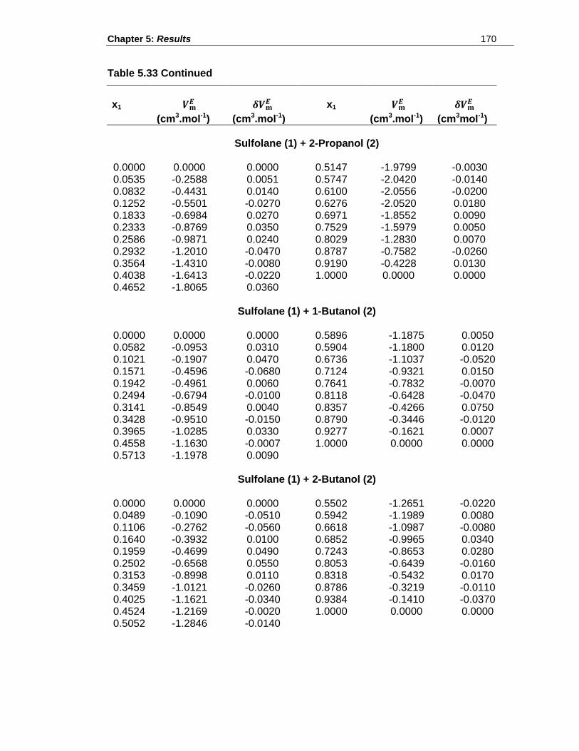
Chapter 5: Results 170
Table 5.33 Continued
x1
x1
(cm3.mol-1) (cm3.mol-1)
(cm3.mol-1) (cm3mol-1)
Sulfolane (1) + 2-Propanol (2)
0.0000 0.0000 0.0000 0.5147 -1.9799 -0.0030 0.0535 -0.2588 0.0051 0.5747 -2.0420 -0.0140 0.0832 -0.4431 0.0140 0.6100 -2.0556 -0.0200 0.1252 -0.5501 -0.0270 0.6276 -2.0520 0.0180 0.1833 -0.6984 0.0270 0.6971 -1.8552 0.0090 0.2333 -0.8769 0.0350 0.7529 -1.5979 0.0050 0.2586 -0.9871 0.0240 0.8029 -1.2830 0.0070 0.2932 -1.2010 -0.0470 0.8787 -0.7582 -0.0260 0.3564 -1.4310 -0.0080 0.9190 -0.4228 0.0130 0.4038 -1.6413 -0.0220 1.0000 0.0000 0.0000 0.4652 -1.8065 0.0360
Sulfolane (1) + 1-Butanol (2)
0.0000 0.0000 0.0000 0.5896 -1.1875 0.0050 0.0582 -0.0953 0.0310 0.5904 -1.1800 0.0120 0.1021 -0.1907 0.0470 0.6736 -1.1037 -0.0520 0.1571 -0.4596 -0.0680 0.7124 -0.9321 0.0150 0.1942 -0.4961 0.0060 0.7641 -0.7832 -0.0070 0.2494 -0.6794 -0.0100 0.8118 -0.6428 -0.0470 0.3141 -0.8549 0.0040 0.8357 -0.4266 0.0750 0.3428 -0.9510 -0.0150 0.8790 -0.3446 -0.0120 0.3965 -1.0285 0.0330 0.9277 -0.1621 0.0007 0.4558 -1.1630 -0.0007 1.0000 0.0000 0.0000 0.5713 -1.1978 0.0090
Sulfolane (1) + 2-Butanol (2)
0.0000 0.0000 0.0000 0.5502 -1.2651 -0.0220 0.0489 -0.1090 -0.0510 0.5942 -1.1989 0.0080 0.1106 -0.2762 -0.0560 0.6618 -1.0987 -0.0080 0.1640 -0.3932 0.0100 0.6852 -0.9965 0.0340 0.1959 -0.4699 0.0490 0.7243 -0.8653 0.0280 0.2502 -0.6568 0.0550 0.8053 -0.6439 -0.0160 0.3153 -0.8998 0.0110 0.8318 -0.5432 0.0170 0.3459 -1.0121 -0.0260 0.8786 -0.3219 -0.0110 0.4025 -1.1621 -0.0340 0.9384 -0.1410 -0.0370 0.4524 -1.2169 -0.0020 1.0000 0.0000 0.0000 0.5052 -1.2846 -0.0140
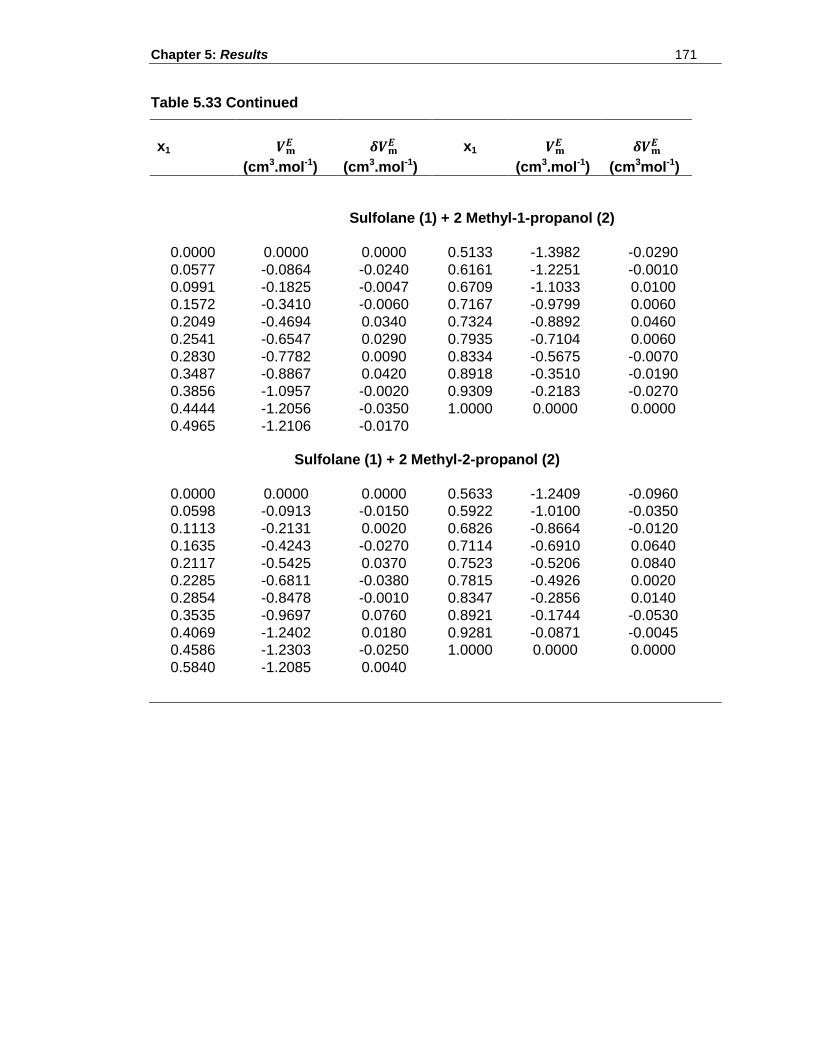
Chapter 5: Results 171
Table 5.33 Continued
x1
x1
(cm3.mol-1) (cm3.mol-1)
(cm3.mol-1) (cm3mol-1)
Sulfolane (1) + 2 Methyl-1-propanol (2)
0.0000 0.0000 0.0000 0.5133 -1.3982 -0.0290
0.0577 -0.0864 -0.0240 0.6161 -1.2251 -0.0010
0.0991 -0.1825 -0.0047 0.6709 -1.1033 0.0100
0.1572 -0.3410 -0.0060 0.7167 -0.9799 0.0060
0.2049 -0.4694 0.0340 0.7324 -0.8892 0.0460
0.2541 -0.6547 0.0290 0.7935 -0.7104 0.0060
0.2830 -0.7782 0.0090 0.8334 -0.5675 -0.0070
0.3487 -0.8867 0.0420 0.8918 -0.3510 -0.0190
0.3856 -1.0957 -0.0020 0.9309 -0.2183 -0.0270
0.4444 -1.2056 -0.0350 1.0000 0.0000 0.0000
0.4965 -1.2106 -0.0170
Sulfolane (1) + 2 Methyl-2-propanol (2)
0.0000 0.0000 0.0000 0.5633 -1.2409 -0.0960
0.0598 -0.0913 -0.0150 0.5922 -1.0100 -0.0350
0.1113 -0.2131 0.0020 0.6826 -0.8664 -0.0120
0.1635 -0.4243 -0.0270 0.7114 -0.6910 0.0640
0.2117 -0.5425 0.0370 0.7523 -0.5206 0.0840
0.2285 -0.6811 -0.0380 0.7815 -0.4926 0.0020
0.2854 -0.8478 -0.0010 0.8347 -0.2856 0.0140
0.3535 -0.9697 0.0760 0.8921 -0.1744 -0.0530
0.4069 -1.2402 0.0180 0.9281 -0.0871 -0.0045
0.4586 -1.2303 -0.0250 1.0000 0.0000 0.0000
0.5840 -1.2085 0.0040
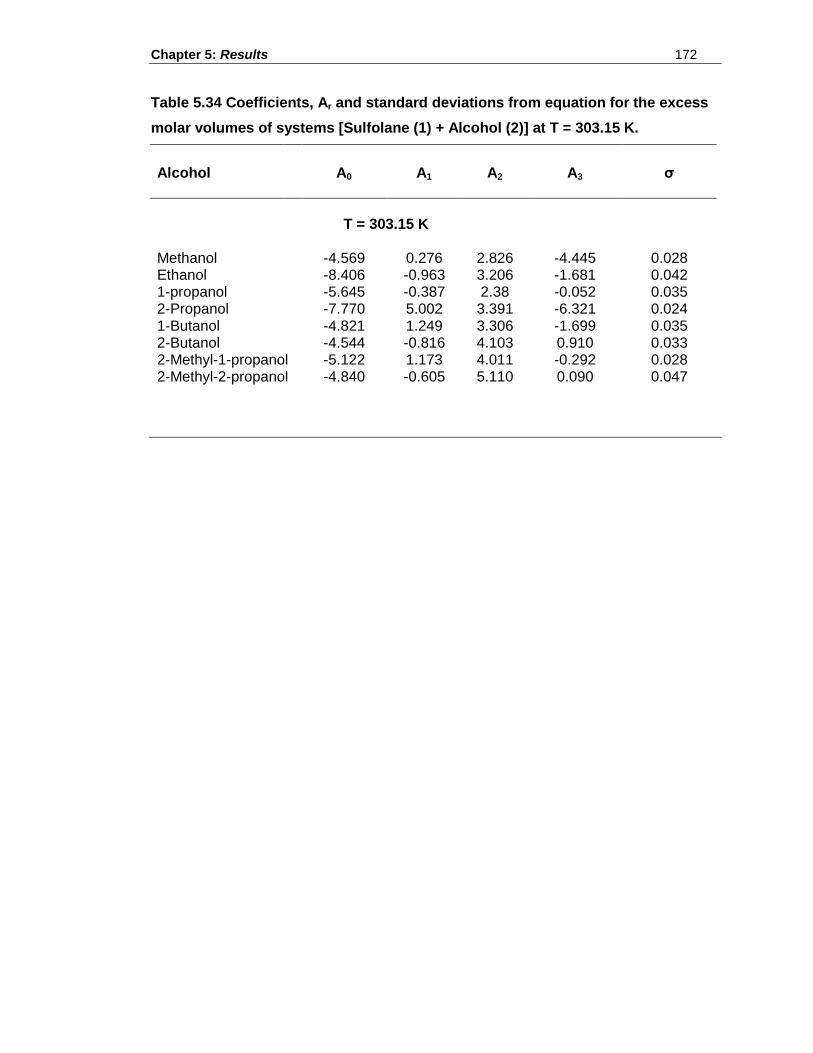
Chapter 5: Results 172
Table 5.34 Coefficients, Ar and standard deviations from equation for the excess
molar volumes of systems [Sulfolane (1) + Alcohol (2)] at T = 303.15 K.
Alcohol
A0 A1 A2 A3 σ
T = 303.15 K
Methanol -4.569 0.276 2.826 -4.445 0.028
Ethanol -8.406 -0.963 3.206 -1.681 0.042 1-propanol -5.645 -0.387 2.38 -0.052 0.035 2-Propanol -7.770 5.002 3.391 -6.321 0.024 1-Butanol -4.821 1.249 3.306 -1.699 0.035 2-Butanol -4.544 -0.816 4.103 0.910 0.033 2-Methyl-1-propanol -5.122 1.173 4.011 -0.292 0.028 2-Methyl-2-propanol -4.840 -0.605 5.110 0.090 0.047
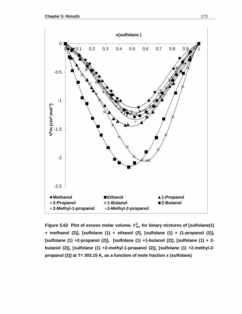
Chapter 5: Results 173
Figure 5.62 Plot of excess molar volume, , for binary mixtures of [sulfolane(1)
+ methanol (2)], [sulfolane (1) + ethanol (2], [sulfolane (1) + (1-propanol (2)],
[sulfolane (1) +2-propanol (2)], [sulfolane (1) +1-butanol (2)], [sulfolane (1) + 2-
butanol (2)], [sulfolane (1) +2-methyl-1-propanol (2)], [sulfolane (1) +2-methyl-2-
propanol (2)] at T= 303.15 K, as a function of mole fraction x (sulfolane)
-2.5
-2
-1.5
-1
-0.5
0
0 0.1 0.2 0.3 0.4 0.5 0.6 0.7 0.8 0.9 1V
Em
(c
m3.m
ol-
1)
x(sulfolane )
Methanol Ethanol 1-Propanol
2-Propanol 1-Butanol 2-Butanol
2-Methyl-1-propanol 2-Methyl-2-propanol
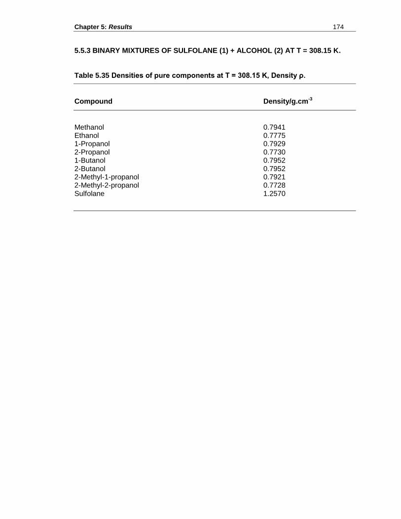
Chapter 5: Results 174
5.5.3 BINARY MIXTURES OF SULFOLANE (1) + ALCOHOL (2) AT T = 308.15 K.
Table 5.35 Densities of pure components at T = 308.15 K, Density ρ.
Compound Density/g.cm-3
Methanol 0.7941 Ethanol 0.7775 1-Propanol 0.7929 2-Propanol 0.7730 1-Butanol 0.7952 2-Butanol 0.7952 2-Methyl-1-propanol 0.7921 2-Methyl-2-propanol 0.7728 Sulfolane 1.2570
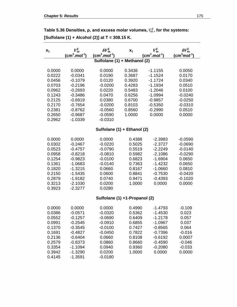
Chapter 5: Results 175
Table 5.36 Densities, ρ, and excess molar volumes, , for the systems:
[Sulfolane (1) + Alcohol (2)] at T = 308.15 K.
x1
x1
(cm3.mol-1) (cm3.mol-1)
(cm3.mol-1) (cm3mol-1)
Sulfolane (1) + Methanol (2) 0.0000 0.0000 0.0000 0.3436 -1.1155 0.0050 0.0222 -0.0341 0.0190 0.3687 -1.1524 0.0170 0.0456 -0.1079 0.0120 0.3920 -1.1724 0.0340 0.0703 -0.2196 -0.0200 0.4283 -1.1934 0.0510 0.0962 -0.2693 0.0220 0.5483 -1.2046 0.0100 0.1243 -0.3486 0.0470 0.6256 -1.0994 -0.0240 0.2125 -0.6919 0.0380 0.6700 -0.9857 -0.0250 0.2170 -0.7654 -0.0200 0.8103 -0.5350 -0.0310 0.2381 -0.8762 -0.0560 0.8560 -0.2990 0.0510 0.2650 -0.9687 -0.0590 1.0000 0.0000 0.0000 0.2962 -1.0339 -0.0310
Sulfolane (1) + Ethanol (2)
0.0000 0.0000 0.0000 0.4388 -2.3983 -0.0590 0.0302 -0.2467 -0.0220 0.5025 -2.3727 -0.0690 0.0523 -0.4757 -0.0790 0.5519 -2.2249 -0.0140 0.0958 -0.8218 -0.0810 0.5982 -2.1086 -0.0290 0.1254 -0.9823 -0.0100 0.6823 -1.6904 0.0650 0.1361 -1.0683 -0.0140 0.7363 -1.4232 0.0650 0.1820 -1.3215 0.0660 0.8167 -1.0660 0.0810 0.2150 -1.5435 0.0600 0.8841 -0.7530 -0.0420 0.2879 -1.9182 0.0740 0.9471 -0.4393 -0.1020 0.3213 -2.1030 0.0200 1.0000 0.0000 0.0000 0.3923 -2.3277 0.0280
Sulfolane (1) +1-Propanol (2)
0.0000 0.0000 0.0000 0.4990 -1.4793 -0.109 0.0386 -0.0571 -0.0320 0.5362 -1.4530 0.023 0.0552 -0.1257 -0.0690 0.6409 -1.2178 0.057 0.0991 -0.2545 -0.0910 0.6855 -1.0967 0.037 0.1370 -0.3545 -0.0100 0.7427 -0.8565 0.064 0.1691 -0.4827 -0.0450 0.7822 -0.7396 -0.016 0.2136 -0.6404 0.0660 0.8108 -0.6192 0.0007 0.2579 -0.8373 0.0860 0.8660 -0.4590 -0.046 0.3354 -1.1094 0.0940 0.9360 -0.2080 -0.033 0.3942 -1.3290 0.0200 1.0000 0.0000 0.0000 0.4145 -1.3591 -0.0180
Chapter 5: Results 176
Table 5.36 Continued
x1
x1
(cm3.mol-1) (cm3.mol-1)
(cm3.mol-1) (cm3mol-1)
Sulfolane (1) + 2-Propanol (2)
0.0000 0.0000 0.0000 0.5147 -1.7376 0.0550 0.0535 -0.1273 0.0400 0.5747 -1.9947 0.0160 0.0832 -0.2039 0.0380 0.6100 -2.0081 0.0430 0.1252 -0.3543 -0.0090 0.6828 -2.0292 0.0040 0.1833 -0.5190 -0.0160 0.6457 -2.0591 -0.1190 0.2333 -0.6579 0.0100 0.7529 -1.5976 -0.0009 0.2586 -0.7818 -0.0190 0.8029 -1.1082 0.0230 0.2759 -0.8593 -0.0290 0.8787 -0.7937 -0.0180 0.3564 -1.1996 -0.0130 0.9190 -0.3486 0.0730 0.3824 -1.4027 -0.0210 1.0000 0.0000 0.0000 0.4652 -1.6577 0.0200
Sulfolane (1) + 1-Butanol (2)
0.0000 0.0000 0.0000 0.5609 -1.2347 0.0240 0.0822 -0.2754 0.0300 0.5960 -1.2104 -0.0020 0.1321 -0.5170 -0.0200 0.6380 -1.1093 -0.0090 0.1871 -0.6924 0.0060 0.6731 -1.1093 -0.0070 0.2194 -0.8208 -0.0070 0.7067 -0.9904 -0.0170 0.2494 -0.9230 0.0360 0.7453 -0.7653 -0.0230 0.3141 -1.1243 -0.0310 0.7780 -0.6590 -0.0002 0.3464 -1.1920 -0.0290 0.8248 -0.4638 0.0320 0.4040 -1.2713 -0.0220 0.8977 -0.2862 0.0140 0.5158 -1.2973 0.0230 1.0000 0.0000 0.0000 0.5543 -1.2336 0.0300
Sulfolane (1) + 2-Butanol (2)
0.0000 0.0000 0.0000 0.4751 -1.3390 -0.0210 0.0588 -0.1382 -0.0200 0.5243 -1.3430 0.0120 0.0821 -0.2351 0.0640 0.5818 -1.2929 -0.0280 0.1064 -0.3585 -0.0400 0.6169 -1.1993 0.0220 0.1552 -0.4658 -0.0390 0.6724 -1.0839 0.0220 0.1850 -0.5247 0.0050 0.7170 -0.9674 -0.0220 0.2533 -0.7839 0.0280 0.7822 -0.7454 0.0120 0.2935 -0.9302 0.0060 0.8179 -0.5372 0.0400 0.3414 -1.1010 0.0300 0.9109 -0.2136 -0.0580 0.3644 -1.1812 -0.0070 1.0000 0.0000 0.0000 0.4140 -1.2838 -0.0290
Chapter 5: Results 177
Table 5.36 Continued
x1
x1
(cm3.mol-1) (cm3.mol-1)
(cm3.mol-1) (cm3mol-1)
Sulfolane (1) + 2- Methyl-1-propanol (2)
0.0000 0.0000 0.0000 0.5133 -1.3430 -0.0080
0.0577 -0.4028 -0.0210 0.6161 -1.1420 0.0040 0.0991 -0.6381 -0.0260 0.6709 -0.9434 0.0080
0.1572 -0.8812 -0.0003 0.7167 -0.8378 0.0070 0.2049 -0.9997 0.0150 0.7324 -0.6102 0.0100
0.2541 -1.1852 0.0210 0.7935 -0.4876 0.0380 0.2830 -1.2546 0.0210 0.8334 -0.3156 -0.0360
0.3487 -1.4072 -0.0090 0.8918 -0.1888 -0.0180 0.3856 -1.4257 -0.0040 0.9309 -0.0620 -0.0010
0.4444 -1.4277 -0.0260 1.0000 0.0000 0.0000 0.4965 -1.3850 -0.0070
Sulfolane (1) + 2- Methyl-2-propanol (2)
0.0000 0.0000 0.0000 0.6259 -1.1970 -0.0420 0.0598 -0.1340 -0.0880 0.6259 -1.0857 0.0190
0.0911 -0.1879 -0.0070 0.6826 -0.8640 0.0020 0.1435 -0.3478 0.0190 0.7114 -0.7596 0.0110
0.1912 -0.4909 0.0670 0.7523 -0.5836 0.0440 0.2254 -0.6438 -0.0220 0.7815 -0.4898 0.0330
0.2854 -0.8521 -0.0140 0.8347 -0.3528 -0.0160 0.3154 -0.9696 0.0760 0.8921 -0.1947 -0.0320
0.3785 -1.1425 -0.0059 0.9281 -0.1087 -0.0300 0.4047 -1.2192 -0.0050 1.0000 0.0000 0.0000
0.4951 -1.3244 -0.0280
Chapter 5: Results 178
Table 5.37 Coefficients, Ar and standard deviations from equation for the excess
molar volumes of systems [Sulfolane (1) + Alcohol (2)] at T = 308.15 K.
A0 A1 A2 A3 σ
T = 308.15 K
Methanol -5.023 -0.915 3.333 0.456 0.036
Ethanol -9.227 -2.550 2.322 2.300 0.060 1-Propanol -5.193 0.454 4.385 1.180 0.065
2-Propanol -7.242 7.038 2.220 -5.771 0.043 1-Butanol -5.075 0.101 0.107 -0.980 0.023
2-Butanol -5.231 2.491 1.407 -3.463 0.030 2-Methyl-1-Propanol -5.584 -2.176 1.914 1.465 0.019
2-Methyl-2-Propanol -4.855 -0.614 5.088 0.918 0.042
Chapter 5: Results 179
Figure 5.63 Plot of excess molar volume, , for binary mixtures of [sulfolane(1)
+ methanol (2)], [sulfolane (1) + ethanol (2)], [sulfolane (1) + (1-propanol (2)],
[sulfolane (1) +2-propanol (2)], [sulfolane (1) +1-butanol (2)], [sulfolane (1) + 2-
butanol (2)], [sulfolane (1) + 2-methyl-1-propanol (2)], [sulfolane (1) +2-methyl-2-
propanol (2)] at T= 308.15 K, as a function of mole fraction x (sulfolane)
-2.5
-2
-1.5
-1
-0.5
0
0 0.1 0.2 0.3 0.4 0.5 0.6 0.7 0.8 0.9 1
VE
m/
cm
3. m
ol-
1
Methanol Ethanol 1-Propanol
2-Propanol 1-Butanol 2-Butanol
2-Methyl-1-propanol 2-Methyl-2-propanol
x (sulfolane)
Chapter 6: Discussion 180
CHAPTER 6
DISCUSSION
6.1 LIQUID- LIQUID EQULIBRIA (LLE)
6.1.1 Ternary systems involving sulfolane (1) + carboxylic acid (2) +
heptane (3) at T = 303.15 K
Previous Work
Mohsen-Nia et al. (2005) studied the ternary mixtures of (solvent + aromatic
hydrocarbon + alkane) at different temperatures from T = 298.15 K to T =
313.15 K. The aromatic hydrocarbon was (toluene or m-xylene) and the alkane
was (n-heptane or n-octane or cyclohexane) whilst the solvent was (sulfolane or
dimethyl sulfoxide or ethylene carbonate). It was reported that the size of the
two phase region decreased with increase in temperature. The selectivity and
distribution coefficient of the solvents used were compared in the study. It was
also found that in the extraction of aromatics from non aromatics, the solvent
with higher selectivity and distribution coefficient was preferred, and based on
calculated partition coefficient and selectivity factor values the superiority of
ethylene carbonate and dimethyl sulfoxide was evident. It was concluded based
on the very strong and bad odour as well as recovery difficulties of dimethyl
sulfoxide, ethylene carbonate was more favourable than dimethylsulfoxide.
Chapter 6: Discussion 181
This work
This work presents new LLE data for the ternary system (sulfolane + acetic acid
or propanoic acid or butanoic acid or 2-methylpropanoic acid or pentanoic acid
or 3-methylbutanoic acid + heptane) at T = 303.15 K.
In binodal curves in figures 5.1-5.6, it can be observed that the solubility of
heptane in (sulfolane + acetic acid or propanoic acid or butanoic acid or 2-
methylpropanoic acid or pentanoic acid or 3-methylbutanoic acid) is dependent
on the type of carboxylic acid. In the ternary systems investigated, the
partitioning of carboxylic acid between heptane and sulfolane is shown to be
dependent on both the length and the structure of the carboxylic acid.
The size of the two phase region decreases with an increase in alkyl group
chain length of the carboxylic acid. Acetic acid has the largest area of the two
phase region as it has shorter carboxylic acid chain length and pentanoic acid or
3-methylbutanoic acid has the smallest area of the two phase region as it has
most number of carbon atoms, of all the investigated carboxylic acids. The
solubility of carboxylic acid in heptane is also inversely related to the size of the
two phase region. In the ternary system investigated, heptane is most soluble in
the systems containing 3-methylbutanoic acid, pentanoic acid, 2-
methylpropanoic acid and butanoic acid.
The single phase homogenous region increases as the carbon chain length of
the carboxylic acid is increased. It can be observed that heptane is most soluble
in the carboxylic acid mixtures with long carbon chains, viz., (3-methylbutanoic
acid + sulfolane) or (pentanoic acid + sulfolane) and least soluble in the
carboxylic acid with short carbon chain (acetic acid + sulfolane).
Chapter 6: Discussion 182
The area of the two phase heterogeneous region for the carboxylic acid mixtures
decrease as the number of carbons in the carboxylic acid chain length
progressively increases. The decreases observed follow the order: acetic acid >
propanoic acid > butanoic acid ~ 2-methylpropanoic acid > pentanoic acid ~3-
methylbutanoic acid.
The mutual solubility of carboxylic acid in sulfolane is dependent on the length
and structure of the carbon chains of the carboxylic acid. Acetic acid, with two
carbons is too short to act as suitable bridging agent between the sulfolane and
heptane. Mutual solubility of the carboxylic acids progressively increases with an
increase in the length of the alkyl chain of the carboxylic acids.
Branching of the carbon chain of carboxylic acid improves the mutual solubility
effect, and both 2-methylpropanoic acid and 3-methylbutanoic acid showed
similar solubility to their corresponding straight chains anologues inspite of their
non-linear structures.
The slope of the tie lines obtained in this investigation showed that all acids
investigated are more soluble in heptane-rich layer than sulfolane- rich layer.
The partitioning of carboxylic acids between the heptane-rich and sulfolane rich
layers for all the systems studied show that all the carboxylic acids are more
soluble in heptane than sulfolane mixtures (Figure 14).
The relatively large two phase region for (the sulfolane + acetic acid + heptane)
system suggested that the entrainer sulfolane has high capacity or loading of
solute per mole fraction of the solvent (sulfolane), that is small quantities of it
would be needed for efficient separation.
The effectiveness of extraction of the carboxylic acid by sulfolane is given by its
selectivity (ω), which is measure of the ability of sulfolane to separate carboxylic
acid from heptane.
Chapter 6: Discussion 183
Selectivity = distribution coefficient of carboxylic acids distribution coefficient of heptane ω = (x2/x3)sulfolane-rich phase (x2/x3)heptane-rich phase
where x2 refers to the mole fraction of the carboxylic acid, and x3 the mole
fraction of heptane.
Table 5.7 gives representative values of the selectivity for the middle of the area
of the measured tie lines for the separation of the carboxylic acids from heptane
using sulfolane. From the selectivity data, it can be observed that the values of
selectivity are all more than 1. Separation of all carboxylic acids from heptane by
extraction therefore feasible. Sulfolane is a good component for separation of
mixtures of heptane and 2-methylpropanoic acid or heptane and 3-
methylbutanoic acid.
The modified Hlavatý, beta (β) and log equations were fitted to the
experimental binodal data. Table 5.1.5 presents the results of fitting of modified
Hlavatý, beta (β) and log equations, Hlavatý function gave the best overall fit
as compare to beta (β) and log function. The NRTL and UNIQUAC models
were used to correlate the experimental tie-lines and to calculate the phase
compositions of the ternary systems. It was found that the NRTL equation fitted
the experimental data significantly better than the UNIQUAC equation.
6.1.2 Ternary systems involving sulfolane (1) + carboxylic acid (2) +
cyclohexane at T = 303.15 K
Previous Work
Rappell et al. (2002) studied the ternary systems of (sulfolane + p-xylene +
cyclohexane), (sulfolane + p-xylene + n-hexane) and (sulfolane + toluene + n-
hexane) at T = 308.15 K and T = 323.15 K.
Chapter 6: Discussion 184
The systems were compared at different temperatures and the results showed
that the two-phase region was enlarged as the temperature was increased
indicating that at higher temperature, sulfolane is more selective solvent for
aromatic compounds. The experimental data were fitted to the NRTL and
UNIQUAC models and NTRL model fitted slightly better than the UNIQUAC
model.
This work
This work presents new LLE data for the ternary system (sulfolane + acetic acid
or propanoic acid or butanoic acid or 2-methylpropanoic acid or pentanoic acid
or 3-methylbutanoic acid + cyclohexane) at T = 303.15 K.
The composition of the mixtures on the binodal curve and mutual solubilities of
sulfolane, carboxylic acid and cyclohexane are given in figure 5.15-5.20. It can
be observed that the solubility of cyclohexane in (sulfolane + acetic acid or
propanoic acid or butanoic acid or 2-methylpropanoic acid or pentanoic acid or
3-methylbutanoic acid) is again dependent on the type of carboxylic acid. The
partitioning of carboxylic acid between cyclohexane and sulfolane is also shown
to be dependent on both the length and the structure of the carboxylic acid.
The solubility of carboxylic acid in (cyclohexane + sulfolane) is dependent on the
alkyl chain length of carboxylic acid. The size of the area of the two phase
region decreases with the increase in the alkyl chain length of carboxylic acid. It
can be observed that acetic acid is observed to have the largest two phase
region are, than all the other carboxylic acids. The single phase homogeneous
region increases as the alkyl group length of the carboxylic acid is increased,
and it can be observed that cyclohexane is most soluble in the carboxylic acid
with long carbon chain (3-methylbutanoic acid + sulfolane) or (pentanoic acid +
sulfolane ) and least soluble in the carboxylic acid with short carbon chain
(acetic acid + sulfolane).
Chapter 6: Discussion 185
The area of the two phase heterogeneous region for the carboxylic acid mixtures
decrease as the number of carbons in the carboxylic acid increases. The
decrease is observed to follow this order: acetic acid > propanoic acid >
butanoic acid ~ 2-methylpropanoic acid > pentanoic acid ~ 3-methylbutanoic
acid.
Mutual solubility of cyclohexane in (sulfolane + carboxylic acid) mixtures is
dependent in the length and structure of the carbon chains of the carboxylic
acid. Acetic acid, with two carbons is too short to act as a suitable bridging agent
between the sulfolane and heptane. Mutual solubility of the carboxylic acids
progressively increases with an increase in the length of the alkyl chain of the
carboxylic acids.
The slope of the tie lines is very important when investigating phase separation
effects. The relative solubility of carboxylic acid in the sulfolane or the alkane is
evident from the tie lines. The gradient of the tie lines obtained in this study
show that all the carboxylic acids investigated are more soluble in cyclohexane
than sulfolane mixtures, as represented on figure 5.21 (a)-(f). From 5.21 (a)-(f) ,
it can also be observed that all carboxylic acids with longer alkyl chain than
acetic acid that were investigated, are more soluble in the cyclohexane rich
layer.
Branching of the carbon chain affects the mutual solubility of both 2-
methylpropanoic acid and 3-methylbutanoic acid. Both showed similar solubility
to their corresponding straight chains anologues inspite of their non-linear
structures. The relatively large two phase region for the (sulfolane + acetic acid
+ cyclohexane) system suggests that the entrainer sulfolane has high capacity
or loading of solute per mole fraction of the solvent (sulfolane), that is small
quantities of it would be needed for efficient separation.
Chapter 6: Discussion 186
Comparing the ternary diagrams for all systems [sulfolane (1) + carboxylic acid
(2) + cylohexane (3)] discussed presently, with the ternary diagrams for
[sulfolane (1) + carboxylic acid (2) + heptane (3)], it was found that replacing
heptane with cyclohexane resulted in a corresponding decrease in the area of
the two-phase heterogeneous region as well as a corresponding decrease in
the slope of tie-lines. This implies that the solvent sulfolane has a higher
solubility, but lower capacity for (carboxylic acid + cyclohexane) mixtures, at the
same temperature. Sulfolane is thus a better solvent for extracting carboxylic
acid from heptane than from cyclohexane.
Table 5.2.5 presents the results of fitting of modified Hlavatý, beta (β) and log
equations to the binodal curves. The Hlavatý function gave the best overall fit as
compare to beta (β) and log function. The NRTL and UNIQUAC models were
used to correlate the experimental tie-lines and to calculate the phase
compositions of the ternary systems. It was found that the NRTL equation fitted
the experimental data significantly better than the UNIQUAC equation.
6.1.3. Ternary systems involving sulfolane (1) + carboxylic acid (2) +
dodecane (3) at T = 303.15 K
Previous Work
Chen-Feng and Wen-Churng (1999) studied the ternary liquid-liquid equilibria of
[alkane (C10/C11/C12/C14) + 1.4 disopropylbenzene + sulfolane] at T = 322.15
K, T = 348.15 K and T = 373.15 K. It was reported that addition of 1.4,
diisopropylbenzene to sulfolane increased the solubility of alkanes in the order
of n-decane > n-dodecane > n-tetradecane, and that the relative mutual
solubility of 1.4-diisopropylbenzene is higher in (n-decane + sulfolane) than in
the (n-dodecane + sulfolane) or (n-tetradecane + sulfolane) mixtures.
Chapter 6: Discussion 187
It was also reported that the size of the two phase region decreased with an
increase in temperature, and from the selectivity data, it can be concluded that
the separation of 1.4-diisopropylbenzene from n-decane, n-dodecane or n-
tetradecane is feasible with sulfolane as a solvent.
This Work
In this work new LLE data have been obtained for (sulfolane + acetic acid or
propanoic acid or butanoic acid or 2-methylpropanoic acid or pentanoic acid or
3-methylbutanoic acid + dodecane) at T = 303.15 K.
The amount of hydrocarbon that is miscible with (sulfolane + carboxylic acid)
mixture is dependent on the carbon number and type of carboxylic acid. In the
ternary systems, illustrated in figures 5.29-5.34 it can be observed that
dodecane is most soluble in the systems containing in pentanoic acid or 3-
methylpropanoic acid. It is found that for a particularly carboxylic acid, the
solubility of dodecane in sulfolane is inversely related to the area of the two
phase region.Solubility of (sulfolane + acetic acid or propanoic acid or butanoic
acid or 2-methylpropanoic acid or pentanoic acid or 3-methylbutanoic acid +
dodecane) is dependent on the type of carboxylic acid.
In the ternary systems investigated, the partitioning of carboxylic acid between
dodecane and sulfolane is shown to be dependent on both the alkyl group chain
length and the structure of the carboxylic acid. In all carboxylic acids the single
phase homogenous region increases as the carbon chain length of the
carboxylic acid is increased, and it is found that dodecane is most soluble in the
carboxylic acid with the long carbon chain (pentanoic acid + sulfolane) mixtures
or (3-methylbutanoic acid + sulfolane) mixtures, and least soluble in the
carboxylic acid with short carbon chain (acetic acid + sulfolane). All carboxylic
acids are more soluble in the dodecane-rich layer than sulfolane-rich layer.
Chapter 6: Discussion 188
Branching of the carbon chain affects the solubility for both 2-methylpropanoic
acid and 3-methylbutanoic acid resulting in both components showing similar
solubilities to their corresponding straight chain anologues.
The shapes of the binodal curves for (sulfolane + carboxylic acid + dodecane)
system show more skewing towards the dodecane axis than that of the
(sulfolane + carboxylic acid + heptane) system. The area of the two phase
heterogeneous region for carboxylic acid mixtures is observed to follow this
order: acetic acid > propanoic acid > butanoic acid ~ 2-methylpropanoic acid >
pentanoic acid ~ 3-methylbutanoic acid.
The relative solubility of an acid in the sulfolane-rich mixture or the alkane- rich
is evident from the tie lines. The gradient of the tie lines obtained in this study
show that all the carboxylic acids are more soluble in dodecane –rich mixture
than in sulfolane-rich mixture. The relatively large two phase region for the
(sulfolane + acetic acid + dodecane) system suggest that the entrainer
sulfolane has a high capacity or loading of solute per mole fraction of the
solvent (sulfolane), that is small quantities of it would be needed for efficient
separation.
The mutual solubility of dodecane in sulfolane and carboxylic acids mixtures is
dependent on the length and structure of the carbon chains of the carboxylic
acid. Mutual solubility of the carboxylic acids progressively increases with an
increase in the length of the alkyl chain of the carboxylic acids. Figure 5.42
shows the plot of relative solubilities of carboxylic acid in sulfolane–rich and
dodecane-rich layers. In the ternary systems investigated, all the carboxylic
acids are more soluble in the dodecane-rich layers than sulfolane-rich layers.
Chapter 6: Discussion 189
The effectiveness of extraction of the carboxylic acids by sulfolane is given by its
selectivity, which is measure of the ability of sulfolane to separate carboxylic
acid from dodecane. The selectivity values obtained are 6 for acetic acid, 2 for
propanoic acid, 6 for butanoic acid, 16 for 2-methylpropanoic acid, 6 for
pentanoic acid and 6 for 3-methylbutanoic acid respectively. From the selectivity
data, it can be observed that the separation of all carboxylic acids from
dodecane by extraction is feasible, and sulfolane is a good solvent for the
separation of mixtures of (3-methylbutanoic acid and dodecane).
Comparing the ternary diagrams for all systems [sulfolane (1) + carboxylic acid
(2) + dodecane (3)] discussed presently, with the ternary diagrams for [sulfolane
(1) + carboxylic acid (2) + heptane (3)], it was found that for all the ternary
systems, replacing heptane with dodecane always results in an increase of the
heterogenous (or 2-phase) region. This implies that the solvent sulfolane has
higher solubility, but lower solvent capacity for (carboxylic acid + heptane)
mixtures at the same temperature and pressure. Sulfolane is thus a better
solvent for extracting carboxylic acids from dodecane , than from heptanes,
whilst sulfolane shows more selectivity for ternary systems with heptanes than
dodecane.
Table 5.19 presents the results of fitting the modified Hlavatý, beta (β) and log
equations to the bimodal curves. The Hlavatý function gave the best overall fit
as compare to beta (β) and log function.
The NRTL and UNIQUAC models were used to correlate the experimental tie-
lines and to calculate the phase compositions of the ternary systems. It was
again found that the NRTL equation fitted the experimental data significantly
better than the UNIQUAC equation.
Chapter 6: Discussion 190
6.1.4 Ternary systems involving sulfolane (1) + alcohol (2) + heptane (3) at
T = 303.15 K
Previous Work
Awwad et al. (2008) presented liquid-liquid equilibria for pseudo-ternary systems
[(sulfolane + 2-ethyoxyethanol) (1) + octane (2) + toluene (3)] at T = 293.15 K. It
was found that the area of the two-phase heterogeneous region decreases with
increase mass fraction of 2-ethoxyethanol in solvent component, that implies
that the existence of more hydrogen bonding interaction between sulfolane and
2-ethoxyethanol resuts in decrease in the area of two-phase region.
It was concluded from the selectivity values that the separation of toluene from
octane by extraction with (sulfolane + mass % 2-ethyoxyethanol) was feasible.
The comparison between experimental selectivity data of (sulfolane + mass %
2-ethyoxyethanol) with that of (sulfolane + 2-methoxyethanol) for the extraction
of toluene from (toluene + octane) mixture at T = 293.15 K was more efficient
using (sulfolane + mass % 2-methoxyethanol).
This work
Liquid- liquid equilibrium data of a new ternary system of (sulfolane + methanol
or ethanol or 1-propanol or 2-propanol or 1-butanol or 2-butanol, or 2-methyl-1-
propanol or 2-methyl-2-propanol + heptane) at T= 303.15 K have been
investigated. The amount of hydrocarbon that is miscible with the (sulfolane +
alcohol) mixture is dependent on the carbon number and type of alcohol. The
ternary diagrams are illustrated on figure 5.43-5.50.
It can be observed that heptane is most soluble in the systems containing (2-
methyl-1-propanol and 2-methyl-2-propanol.
Chapter 6: Discussion 191
It is evident that the amount of hydrocarbon that is miscible with the alcohols is
very much dependent on the alkyl chain of the alcohol and the location of the
hydroxyl group (-OH) of the alcohol.
It is found that for particular alcohols the solubility of heptane in sulfolane is
inversely related to the area of the two phase region. Solubility of alcohols
investigated is dependent on the type of alcohol, the partitioning of alcohol
between heptane and sulfolane is shown to be also dependent on both the
length and the structure of the alcohol. The single phase homogenous region
increases as the alkyl chain length of the alcohol is increased, and it is found
that heptane is most soluble in the alcohol with long carbon chain( 2-methyl-1-
propanol + sulfolane ) or (2-methyl-2-propanol + sulfolane) and least soluble in
the alcohol with short carbon chain (methanol + sulfolane).
Figure 5.60 shows a plot of the relative solubities of the alcohols in the
sulfolane-rich and heptane-rich layers. All the alcohols are more soluble in the
heptane layer than sulfolane layer. In case of methanol and ethanol, the
hydrogen bonding with sulfolane is stronger since these alcohols are completely
miscible with sulfolane. However, propanol and butanol alcohols are partially
miscible with sulfolane because the hydrocarbon part of these alcohol molecules
show diminished interaction with sulfolane even though sulfolane molecule form
strong hydrogen bonds (Hwang et al.,2008)
From Figure 5.51, the area of the two phase heterogeneous region for alcohol
mixtures increase is observed to follow this order: 2-methyl-1-propanol ~ 2-
methyl-2-propanol < 1-butanol ~ 2-butanol < ethanol < 1-propanol ~ 2-propanol
< methanol.
Chapter 6: Discussion 192
The relative solubility of an alcohol in the sulfolane or the alkane is evident from
the tie lines. The gradient of the tie lines obtained in this study show that all the
alcohols are more soluble in sulfolane than heptane mixture. The relatively large
two phase region for the sulfolane + methanol + heptane system suggest that
the entrainer sulfolane has high capacity or loading of solute per mole fraction
of the solvent (sulfolane), that is small quantities of it would be needed for
efficient separation.
Mutual solubility of heptane in sulfolane is dependent in the length and structure
of the carbon chains of the alcohol. Mutual solubility of the alcohols
progressively increases with an increase in the length of the alkyl chain of the
acids but it is shown that branching does not increase solubility appreciably.
The effectiveness of extraction of the carboxylic by sulfolane is given by its
selectivity, which is measure of the ability of sulfolane to separate alcohol from
heptane. The selectivity values obtained are 5 for methanol, 8 for ethanol, 3 for
1-propanol, 6 for 2-propanol, 11 for 1-butanol, 5 for 2-butanol, 8 for 2-methyl-
1-propanol and 9 for 2-methyl-2-propanol respectively. From the selectivity
data, it can be observed that the separation of all alcohols from heptane by
extraction is feasible. Sulfolane is a good solvent for the separation of the
mixtures of alcohols from heptane.
Comparing the ternary diagrams for all systems [sulfolane (1) + alcohol (2) +
heptane (3)] discussed presently, with the ternary diagrams for [sulfolane (1) +
carboxylic acid (2) + heptane (3), there was an increase in two-phase
heterogeneous region as well the slope of tie-linesfrom the former systems. This
implies that the solvent sulfolane has a higher solubility, but lower solvent power
or capacity for (carboxylic acid + heptane) mixtures, at the same temperature
and pressure. Sulfolane is thus a better solvent for extracting alcohols from
heptane than carboxylic acids from heptane.
Chapter 6: Discussion 193
Table 5.26 presents the results of fitting of modified Hlavatý, beta (β) and log
equations, Hlavatý function gave the best overall fit as compare to beta (β) and
log function. The NRTL and UNIQUAC models were used to correlate the
experimental tie-lines and to calculate the phase compositions of the ternary
systems. It was found that overall the NRTL equation fitted the experimental
data significantly better than the UNIQUAC equation.
6.2 EXCESS MOLAR VOLUMES
6.2.1 Mixtures of (sulfolane + alcohols) at T = 298.15 K
Previous work
Chen et al. (2005) presented viscosities and densities for binary mixtures of n-
methylpiperazine with methanol, ethanol, n-propanol, isopropanol, n-butanol and
isobutanol at T = 293.15 K, T = 298.15 K and T = 303.15 K and atmospheric
pressure. It was found that all the investigated systems exhibited very large
positive values of viscosity deviation and excess Gibbs energy, and that excess
molar volumes were negative over the entire composition range. It was reported
that the deviations were attributed to the strong cross association between the
alkanol and n-methylpiperazine molecules through the hydrogen bond of O-H-N.
It was also reported the temperature had significant effect on of viscosity
deviation and relatively slight effect on the excess molar volumes and excess
Gibbs energy.
Chapter 6: Discussion 194
This work
Excess molar volumes for eight binary mixture of (sulfolane + methanol or
ethanol or 1-propanol or 2-propanol or 1-butanol or 2-butanol or 2-methyl-1-
propanol or 2-methyl-2-propanol) at T = 298.15 K have been determined. The
aim of the investigation was to determine the influence the increasing carbon
chain length of the alcohols on the excess molar volumes ( )
The excess molar volumes are the results of the intermolecular interactions that
are due to the difference between the real and ideal molar volumes. Positive
excess molar volumes are the result of the intermolecular dissociation effect
resulting in bond breaking of the pure solvents. The negative excess molar
volumes are due to association between the solutes molecules and packing.
Table 5.30 show that the excess molar volume values are negative over the
entire mole fraction range for all the binary mixtures studied in present work. The
negative excess molar volumes indicate that the packing degree in these mixed
liquids is higher than in the pure species and in their idealized mixtures.
Negative values of excess molar volume suggest a more efficient packing or
attractive interaction occurred when sulfolane and alcohol molecular liquids were
mixed.
The negative excess molar volumes can be also explained in terms of two
opposing effects, expansion in volume due to mutual loss of dipolar association
as well as the difference in the size and shape of component molecules and
contraction in volume comes from dipole-induced dipole dipole-dipole
interactions and donor-acceptor interactions between unlike molecule (Yang-Xin
et al.,1998).
Chapter 6: Discussion 195
Assuming that the energy associated with orientational order for all pure
alcohols is the same order, the variation in excess molar volume of these
mixtures will be due to the variation in magnitude of specific energy in these
mixtures. There are specific electron donor interactions between sulfolane and
alcohols (Yang-Xin et al., 1998).
A negative excess molar volume could be due to an association of the species
involved, bringing the molecules closer together, resulting in decrease or
contraction of volume, or it could be due to the sympathetic packing effect of the
molecule. Packing effects could also contribute either positively or negatively to
the excess volumes.The negative excess molar results obtained are due to both
the intermolecular effects as well as packing effect (Redhi, 2003). The excess
molar volumes curves have a minima ranging from between -0.6257 cm3.mol-1
to -2.2357 cm3.mol-1 at T = 298.15 K.
The excess molar volume at equimolar composition for the binary systems
(sulfolane + methanol or ethanol or 1- propanol or 2-propanol or 1-butanol or 2 -
butanol or 2- methyl-1-propanol or 2-methyl-2-propanol) at T = 298.15 K, T =
303.15 K and T= 308.15 K is tabulated on Table 6.1.
The excess molar volume is most negative in the case of ethanol and 2-
propanol at all the temperatures investigated. The magnitude of excess volumes
of alcohols decreases in the following order ethanol > 2propanol > 2-methy-1-
propanol > 1-butanol > 2-methyl-2-propanol > methanol > 2-butanol >1-propanol
at T = 298.15 K.
From figure 5.62, it can be observed that most of the curves of the alcohols are
skewing towards the region of high mole fraction of sulfolane or low mole
fraction of the alcohol. The same trend is observed on most of alcohols
investigated.
Chapter 6: Discussion 196
The interaction between the unlike molecules seems to be stronger than the
intra-molecular interactions, leading to negative values of excess molar
volumes. The kinetic energy of the molecules increases when the temperature
increases, and this lead to a decrease of their interaction as the contraction in
volume decreases that is excess molar volumes increases (Wang et al, 2004).
The resulting differences in energies of the molecules and packing effects
disrupts the ordered structure of pure component during the formation of the
mixture leading to negative effect observed on excess molar volume when as
order formation in the mixture leading to negative contribution to the excess
molar volume (Iloukhani et al., 2006).
For each binary mixture, excess molar volume data were fitted to the Redlich–
Kister equation to correlate the composition dependence of the excess property
using equation 4.10. The parameters A0, A1, A2, A3 and the standard deviations
for each binary mixture are shown on table 5.31.
6.2.2 Mixtures of (sulfolane + alcohols) at T = 303.15 K
Previous work
Kinart et al., (2007) presented densities and relative permittivities of the binary
mixtures of sulfolane with ethylene glycol, diethylene glycol, triethylene glycol
and tetraethylene glycol as has been measured as function of composition at T
= 303.15 K.
It was reported that the excess molar volumes were negative over the
composition range for all systems, the value of molar excess volume became
more negative as the number of oxyethylene groups in the glycols increased.
Chapter 6: Discussion 197
It was concluded that the globular molecules of sulfolane had no significant
intermolecular hydrogen bonding capability in pure liquid, and that molecules of
glycols are self-associated liquids though inter- and intramolecular hydrogen
bonding. It was found that formation of intramolecular hydrogen bonds in the
liquid ethylene glycols was more favourable when the molecules of these
solvents are in the gauche formations.
This work
Excess molar volumes for binary mixture of sulfolane and alcohols (methanol or
ethanol or 1-propanol or 2-propanol or 1-butanol or 2-butanol or 2-methyl-2-
propanol or 2-methyl-1-propanol) at T = 303.15 K have been investigated. Table
5.33 shows that the excess molar volume values are negative over the entire
mole fractions range, for all the binary mixtures studied in present work.
Negative values of excess molar volume suggest that a more efficient packing or
attractive interaction occurred when sulfolane and alcohol molecular liquids were
mixed. The results are graphically represented in figure 5.62.
The negative excess molar volumes indicate that the packing degree in these
mixed liquids is higher than in the pure species and in their idealized mixtures,
suggesting that the specific intermolecular interaction such as hydrogen bonding
and dipolar interactions of any kind are effective among these chemical species
(Kinart et al., 2007). The molecular interactions between the mixing species
mainly depend upon the composition, the different molecular sizes and the
shapes of the components and experimental temperature.
The globular molecules of sulfolane have no significant intermolecular hydrogen
bonding capability in pure liquid, on the other hand, the molecules of alcohols
are self-associated liquids through inter and intermolecular hydrogen bonding.
Chapter 6: Discussion 198
The free sulfolane and alcohol molecules may interact by dipole-dipole forces
and or intermolecular hydrogen bonds forming the mixed intermolecular
complexes. Similar structural effects have been observed in binary of sulfolane
+ aliphatic alcohol (normal and branched chain) (Kinart et al., 2007).
From Table 6.1, it is found that the excess molar volumes curves of sulfolane
and alcohols have a minima ranging from -1.1461 cm3.mol-1 to -2.1016 cm3.mol-1
at T = 303.15 K. The excess molar volume values are most negative in the case
of ethanol and 2- propanol. The magnitude of excess molar volumes of alcohols
decreases in the following order ethanol > 2-propanol > 1-propanol > 2-methyl-
1-propanol > 1-butanol > methanol > 2-butanol at T = 303.15 K.
For each binary mixture, excess molar volume data were fitted to the Redlich–
Kister equation to correlate the composition dependence of the excess property
using equation 4.10. The parameters A0, A1, A2, A3 and the standard deviations
for each binary mixture are shown on table 5.34.
6.2.3 Mixtures of (sulfolane + alcohols) at T = 308.15 K
Previous work
Wang et al, (2004) presented the excess molar of (cyclohexanone + benzene or
toluene or ethylbenzene or styrene) were obtained from the densities over the
composition range at temperature T = ( 293.15 K, 303.15 K, 313.15 K, 323.15 K,
333.15 K, 343.15 K and 353.15 K) and atmospheric pressure.
It was found that the excess molar volumes had shifted in a regular way with
the increasing temperature from T = 293.15 K to 313.15 K. It was reported that
in each system, a slight decrease in excess molar volumes over the whole mole
fraction range was noticeable with increasing temperature.
Chapter 6: Discussion 199
From the comparison of the minimum values of excess molar volumes for the
three mixtures containing an aromatic hydrocarbon at the same temperature. It
was concluded styrene was the most favourable one to form close packing with
cylohexanone.
This work
Excess molar volumes for binary mixtures of (sulfolane + methanol or ethanol or
1-propanol or 2-propanol or 1-butanol or 2-butanol or 2-methyl-1-propanol or 2-
methyl-2-propanol) at T = 308.15 K have been determined.
Table 5.36 show that the excess molar volume values are negative over the
entire mole fraction range for all the binary mixtures studied in the present work.
The negative excess molar volumes indicate that the packing degree in these
mixed liquids is higher than in the pure species and in their idealized mixtures.
Negative values of excess molar volume suggest a more efficient packing or
attractive interaction occurred when sulfolane and alcohol molecular liquids were
mixed.
From figure 5.63 it can be observed that most of the curves of the alcohols are
slightly skewed towards the region of high mole fraction of sulfolane or low mole
fraction of the alcohol. The interaction between the unlike molecules seems to
be stronger than the intramolecular interactions, leading to negative values of
excess molar volumes. The kinetic energy of the molecules increases when the
temperature increases, that lead to decrease of their interaction as the
contraction in volume decreases, that is the excess molar volumes increases
(Wang et al., 2004).
The excess molar volumes curves have a minima ranging from -1.2016 cm3.mol-
1 to - 2.3983 cm3.mol-1 at T = 308.15 K.
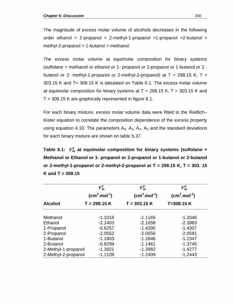
Chapter 6: Discussion 200
The magnitude of excess molar volume of alcohols decreases in the following
order ethanol > 2-propanol > 2-methyl-1-propanol >1-propanol >2-butanol >
methyl-2-propanol > 1-butanol > methanol.
The excess molar volume at equimolar composition for binary systems
(sulfolane + methanol or ethanol or 1- propanol or 2-propanol or 1-butanol or 2 -
butanol or 2- methyl-1-propanol or 2-methyl-2-propanol) at T = 298.15 K, T =
303.15 K and T= 308.15 K is tabulated on Table 6.1. The excess molar volume
at equimolar composition for binary systems at T = 298.15 K, T = 303.15 K and
T = 308.15 K are graphically represented in figure 6.1.
For each binary mixture, excess molar volume data were fitted to the Redlich–
Kister equation to correlate the composition dependence of the excess property
using equation 4.10. The parameters A0, A1, A2, A3 and the standard deviations
for each binary mixture are shown on table 5.37.
Table 6.1: at equimolar composition for binary systems (sulfolane +
Methanol or Ethanol or 1- propanol or 2-propanol or 1-butanol or 2-butanol
or 2-methyl-1-propanol or 2-methyl-2-propanol at T = 298.15 K, T = 303. 15
K and T = 308.15
(cm3.mol-1) (cm3.mol-1) (cm3.mol-1)
Alcohol T = 298.15 K T = 303.15 K T=308.15 K
Methanol -1.1016 -1.1165 -1.2046 Ethanol -2.1403 -2.1658 -2.3983 1-Propanol -0.6257 -1.4290 -1.4307 2-Propanol -2.0552 -2.0556 -2.0591 1-Butanol -1.1803 -1.2846 -1.2347 2-Butanol -0.8299 -1.1461 -1.3745 2-Methyl-1-propanol -1.3921 -1.3982 -1.4277 2-Methyl-2-propanol -1.1109 -1.2409 -1.2443
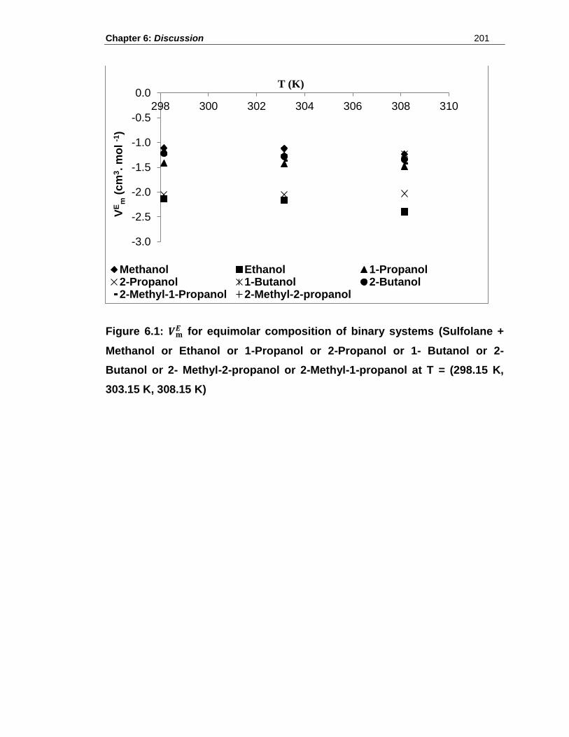
Chapter 6: Discussion 201
Figure 6.1: for equimolar composition of binary systems (Sulfolane +
Methanol or Ethanol or 1-Propanol or 2-Propanol or 1- Butanol or 2-
Butanol or 2- Methyl-2-propanol or 2-Methyl-1-propanol at T = (298.15 K,
303.15 K, 308.15 K)
-3.0
-2.5
-2.0
-1.5
-1.0
-0.5
0.0
298 300 302 304 306 308 310V
Em
(cm
3.
mo
l -1
)
Methanol Ethanol 1-Propanol2-Propanol 1-Butanol 2-Butanol2-Methyl-1-Propanol 2-Methyl-2-propanol
T (K)
Chapter 7: Conclusions 202
CHAPTER 7
CONCLUSIONS
In this chapter, the experimental work presented in chapter 5 is summarized.
7.1 TERNARY SYSTEM LIQUID-LIQUID EQUILIBRIA
Precise new liquid- liquid equilibria data are presented for the following
systems at 303.15 K.
Sulfolane (1) + Carboxylic Acid (2) + Heptane (3) at T = 303.15 K
Sulfolane (1) + Carboxylic Acid (2) + Cyclohexane (3) at T = 303.15 K
Sulfolane (1) + Carboxylic Acid (2) + Dodecane (3) at T = 303.15 K
Sulfolane (1) + Alcohol (2) + Heptane (3) at T = 303.15 K
7.1.1 Liquid- liquid equilibria for mixtures of sulfolane (1) + carboxylic
acid (2) + heptane (3)
Liquid-liquid equilibria for the ternary system (sulfolane + acetic acid or
propanoic acid or butanoic acid or 2-methylpropanoic acid or butanoic acid or
3-methylbutanoic acid + heptane) were investigated at T = 303.15 K.
The solubility of carboxylic acid in (heptane + sulfolane) mixtures is inversely
related to the size of the two phase region. The area of the two phase
heterogeneous region for the carboxylic acid mixtures decrease as the
number of carbon in the carboxylic acid increases. The decrease is observed
to follow the order: acetic acid > propanoic acid > butanoic acid ~ 2-
methylpropanoic acid > pentanoic acid ~3-methylbutanoic acid.
Chapter 7: Conclusions 203
The slope of the tie lines obtained in this investigation showed that all acids
are more soluble in heptane-rich layers than in sulfolane-rich layers. The
partitioning of carboxylic acids between the heptane-rich and sulfolane rich
layers for all the systems studied show that all the carboxylic acids are more
soluble in heptane than in sulfolane.
The separation of a carboxylic acid from heptane by extraction with sulfolane
is feasible, as can be ascertained from the selectivity data in table 5.1.7. The
selectivity values are all greater than 1. Sulfolane has the highest solvent
capacity for the extraction of acetic acid, than any of the other carboxylic
acids.
The modified Hlavatý, beta (β) and log γ equations were fitted to the
experimental binodal data. The Hlavatý function gave the best overall fit
when compare to the beta (β) and log γ function.
It was found that the NRTL equation fitted the experimental data significantly
better than the UNIQUAC equation.
7.1.2 Liquid- liquid equilibria for mixtures of sulfolane (1) + carboxylic
acid (2) + cyclohexane (3)
Liquid-liquid equilibria for the ternary system (sulfolane + acetic acid or
propanoic acid or butanoic acid or 2-methylpropanoic acid or butanoic acid or
3-methylbutanoic acid + cyclohexane) was investigated at T = 303.15 K.
The relative solubility of carboxylic acid in the sulfolane or the alkane mixture
is evident from the tie lines. The gradient of the tie lines obtained in this study
show that all the carboxylic acids investigated are more soluble in
cyclohexane than sulfolane mixtures.
Chapter 7: Conclusions 204
From figure 5.21 (a) - (f), it can be observed that the gradient of the tie-lines
for 2-methylpropanoic is significantly greater that those for butanoic acid.
This could be attributed to the solubilising effect of the two electron realising
methyl groups on the terminal carbon of the 2-methylpropanoic acid as
opposed to its straight chain isomer. A similar effect is noted for 3-
methylbutanoic acid when compared to pentanoic acid.
The area of the two phase heterogeneous region for the carboxylic acid
mixtures decrease as the number of carbon in the carboxylic acid increases.
The decrease is observed to follow this order: 3-methylbutanoic acid <
pentanoic acid< 2–methylpropanoic acid < butanoic acid < propanoic acid <
acetic acid.
From the selectivity data, it can be concluded that the separation of all
carboxylic acids from cyclohexane by extraction is feasible. It can also be
concluded that sulfolane is a good component for separation of the mixtures
of (cyclohexane and butanoic acid) and to a lesser extent or (cyclohexane
pentanoic acid).
The modified Hlavatý, beta (β) and log γ equations were fitted to the
experimental binodal data. The Hlavatý function again gave the best overall
fit as compared to beta (β) and log γ function.
Chapter 7: Conclusions 205
7.1.3 Liquid- liquid equilibria for mixtures of sulfolane (1) + carboxylic
acid (2) + dodecane (3)
Liquid-liquid equilibria for the ternary system (sulfolane + acetic acid or
propanoic acid or butanoic acid or 2-methylpropanoic acid or butanoic acid or
3-methylbutanoic acid + dodecane) were investigated at T = 303.15 K.
Liquid-liquid equilibria for the ternary system: sulfolane + carboxylic acids
(acetic acid, propanoic acid, butanoic acid, 2-methylpropanoic acid, butanoic
acid and 3-methylbutanoic acid) + dodecane were investigated at T = 303.15
K. In the ternary systems investigated, the partitioning of carboxylic acid
between dodecane and sulfolane is shown to be dependent on both the alkyl
chain length and the structure of the carboxylic acid.
The single phase homogenous region increases as the carbon chain length
of the carboxylic acid is increased, and it is found that dodecane is most
soluble in the carboxylic acid with long carbon chain (pentanoic acid +
sulfolane) or (3-methylpropanoic acid + sulfolane) and least soluble in the
carboxylic acid with short carbon chain (acetic acid + sulfolane). All
carboxylic acids are more soluble in dodecane layer than sulfolane layer.
Branching of the carbon chain improves the solubility of both 2-
methylpropanoic acid and 3-methylbutanoic acid and they it show similar
solubilities to their corresponding straight chains anologues. The area of the
two phase heterogenous region for carboxylic acid mixtures increase in the
order: acetic acid > propanoic acid > butanoic acid ~ 2-methylpropanoic acid
> pentanoic acid ~ 3-methylbutanoic acid.
Chapter 7: Conclusions 206
The effectiveness of extraction of the carboxylic by sulfolane is given by its
selectivity, which is measure of the ability of sulfolane to separate carboxylic
acid from dodecane. Table 5.21 shows that all the selectivity values are
greater than 1, implying that separation is feasible in all cases and that
sulfolane is an especially good component for separation of (dodecane and
2-methylpropanoic acid) mixtures.
The modified Hlavatý, beta (β) and log γ equations were fitted to the
experimental binodal data. The Hlavatý function again gave the best overall
fit as compare to beta (β) and log γ function.
It was found that the NRTL equation correlated the experimental tie line data
significantly better than the UNIQUAC equation.
7.1.4 Liquid- liquid equilibria for mixtures of sulfolane (1) + alcohol (2) +
heptane (3)
Liquid-liquid equilibria for the ternary system (sulfolane + methanol or ethanol
or 1-propanol or 2-propanol or 1-butanol or 2-butanol or 2-methyl-1-propanol
or 2-methyl-2-propanol + heptane) were investigated at T = 303.15 K.
Solubility of heptane in (sulfolane + alcohol) mixtures is very much
dependent on the carbon chain number and the type of the alcohol. The
single phase homogenous region increases as the alkyl chain length of the
alcohol is increased, and it is found that heptane is most soluble in the
alcohol with long carbon chain (2-methyl-1-propanol + sulfolane ) or (2-
methyl-2-propanol + sulfolane) and least soluble in the alcohol with short
carbon chain (methanol + sulfolane). All the alcohols are more soluble in
heptane layer than sulfolane layer.
Chapter 7: Conclusions 207
The gradient of the tie lines for 1-propanol and 2-propanol show considerable
difference. This could be attributable to greater solubilizing effect of the
secondary alcohol (2-propanol), as opposed to primary alcohol (1-propanol).
Branching of the carbon chain improves the mutual solubility effect and 2-
methyl-2-propanol and to a lesser extent 2-methyl-1-propanol serve as good
bridging agents.
The effectiveness of extraction of the alcohols from heptane by sulfolane is
given by its selectivity, which is measure of the ability of sulfolane to separate
alcohols from heptane. Table 5.28 shows that the selectivity values are in all
cases are greater than 1, and separation is therefore feasible. It can also be
concluded that sulfolane is a good component for separation of (heptane + 1-
butanol) mixtures.
The modified Hlavatý, beta (β) and log γ equations were fitted to the
experimental binodal data. The Hlavatý function gave the best overall fit as
compare to beta (β) and log γ function.
It was found that the NRTL equation correlated the experimental tie-line data
significantly better than the UNIQUAC equation.
7.2 EXCESS MOLAR VOLUMES
The excess molar volumes for binary mixtures of (sulfolane + alcohol) have
been determined. The systems are
Binary mixtures of sulfolane and alcohols (methanol or ethanol or 1-
propanol or 2-propanol or 1-butanol or 2-butanol or 2-methyl-1-
propanol or 2-methyl-2-propanol ) at T = 298.15 K
Binary mixtures of sulfolane and alcohols (methanol or ethanol or 1-
propanol or 2-propanol or 1-butanol or 2-butanol or 2-methyl-1-
propanol or 2-methyl-2-propanol) at T = 303.15 K.
Chapter 7: Conclusions 208
Binary mixtures of sulfolane and alcohols (methanol or ethanol or 1-
propanol or 2-propanol or 1-butanol or 2-butanol or 2-methyl-1-
propanol or 2-methyl-2-propanol) at T = 308.15 K.
7.2.1 Mixtures of (sulfolane + alcohols) at T = 298.15 K
Excess molar volume for the binary mixtures of sulfolane and alcohols
(methanol or ethanol or 1-propanol or 2-propanol or 1-butanol or 2-butanol or
2-methyl-1-propanol or 2-methyl-2-propanol) at T = 298.15 K has been
determined.
The excess molar volume values are negative over the entire mole fraction
range for all the binary mixtures studied in this work. Negative values of
excess molar volume suggest a more efficient packing or attractive
interaction occurred when sulfolane and alcohol molecular liquids were
mixed. Negative excess molar volume could be due to an association of the
species involved, bringing the molecules closer together, resulting in
decrease or contraction of volume, or it could be due to the sympathetic
packing effect of the molecule.
The excess molar volume is most negative in the case of ethanol and 2-
propanol at all the temperatures investigated. At T = 298.15 K, the magnitude
of excess volumes of alcohols decreases in the following order ethanol > 2-
propanol > 1-propanol > 2-methyl-1-propanol > 2-butanol > 2-methyl-2-
propanol > 1-butanol >methanol.
Figure 5.63 is the graphical representation of excess molar volume for the
binary mixtures of (sulfolane + alcohol) at T = 298.15 K. It can be observed
that most of the curves of the alcohols are skewing towards the region of high
mole fraction of sulfolane or low mole fraction of the alcohol.
Chapter 7: Conclusions 209
The excess molar volumes curves of sulfolane and alcohols have a minima
ranging from -1.1121 cm3.mol-1 to -2.1405 cm3.mol-1 at T = 298.15 K . The
excess molar volume values are most negative in the case of ethanol and 2-
propanol. The free sulfolane and alcohol molecules may interact by dipole-
dipole forces and intermolecular hydrogen bonds forming the mixed
intermolecular complexes. Similar structural effects have been observed in
binary mixtures of (sulfolane + aliphatic alcohol) involving normal and
branched aliphatic chain.
7.2.2 Mixtures of (sulfolane + alcohols) at T = 303.15 K
The excess molar volumes of the binary mixtures of sulfolane and alcohols
(methanol or ethanol or 1-propanol or 2-propanol or 1-butanol or 2-butanol or
2-methyl-1-propanol or 2-methyl-2-propanol) at T = 303.15 K have been
determined.
Table 5.33 show that the excess molar volume values are again negative
over the entire mole fraction range for all the binary mixtures studied in the
present work. Negative values of excess molar volume suggest a more
efficient packing or attractive interaction occurred when sulfolane and alcohol
molecular liquids were mixed. The results are graphically represented in
figure 5.62.
The excess molar volumes curves of sulfolane and alcohols have a minima
ranging from -1.1165 cm3.mol-1 to -2.1658 cm3.mol-1 at T = 303.15 K. The
excess molar volume values are most negative in the case of ethanol and 2-
propanol. The magnitude of excess molar volumes of alcohols decreases in
the following order ethanol > 2-propanol > 1-propanol > 2-methyl-1-propanol
> 2-butanol > 2-methyl-2-propanol > 1-butanol > methanol at T = 303.15 K.
Chapter 7: Conclusions 210
Comparing the magnitude of excess molar volume minima for binary
mixtures of (sulfolane + alcohol) at T = 298.15 K to the binary mixtures of
(sulfolane + alcohol) at T = 303.15 K showed corresponding decrease in the
excess molar volume minima over the entire range of mole fraction range
with the increase in experimental temperature.
7.2.3 Mixtures of (sulfolane + alcohols) at T = 308.15 K
The excess molar volumes of the binary mixtures of sulfolane and alcohols
(methanol or ethanol or 1-propanol or 2-propanol or 1-butanol or 2-butanol or
2-methyl-1-propanol or 2-methyl-2-propanol) at T = 308.15 K have been
determined.
The excess molar volume values are again negative over the entire mole
fractions range for all the binary mixtures studied in the present work.
Negative values of excess molar volume suggest a more efficient packing or
attractive interaction occurred when sulfolane and alcohol molecular liquids
were mixed. The results are graphically represented in figure 5.63.
The excess molar volumes curves have a minima ranging from -1.2319
cm3.mol-1 to - 2.3983 cm3.mol-1 at T = 308.15 K. The excess molar volume of
alcohols decreases in the following order ethanol > 2-propanol > 1-propanol
>2-methyl-1-propanol > 2-butanol > 2-methyl-2-propanol > 1-butanol >
methanol.
Comparing the magnitude of excess molar volume minima for binary mixture
of (sulfolane + alcohol) at T = 303.15 K to the binary mixture of (sulfolane +
alcohol) at T = 308.15 K showed the decrease in the excess molar volume
minima for the latter system at T = 303.15 K over the entire range of mole
fraction range.
C h a p t e r 8 : R e f e r e n c e s 211
CHAPTER 8
REFERENCES
Abrams D., Prausnitz J.M., AIChEJ, 1975, 21, 116.
Aguila-Hernandez J., Trejo A., Garcia F.B., Molnar R., Fluid Phase Equlibria,
2008, 267, 172 -180.
Ahamd S.A., Tanwar R.S., Gupta R.K., Khanna A., Fluid Phase Equilibria,
2004, 220, 189 -198.
Awwad A., Al-Dujaili A. H, Al-Haideri A. A., Essa Hatim M., Fluid Phase
Equilibria, 2008, 270, 10-14.
Ahmad A.B., Othham M. R., ScienceAsia, 2010, 81-84.
Benoit R.L., Charbonneau J., Canadian Journal of Chemistry, 1969, 47,
4195.
Bertleff W., Roeper M., Sava X., “Carbonylation” in Ullmann‟s Encyclopedia
of Chemical Technology Wiley, 2003, 217.
Bondi A., Physical Properties of Molecular Crystals, Liquid and Glasses,1968
Wiley New York.
Bowen B. H., Irwin W. M., Coal Gasification & Fischer-Tropsch, Indiana
Center for Coal Technology Research Report, 2006.
Briggs S.W., Commings E.W., In Eng. Chem, 1943, 35, 411.
C h a p t e r 8 : R e f e r e n c e s 212
British Colombia Ministry of Water, Land and Air Protection Report, Water
Quality Guidelines for Sulfolane, 2003, Komex International, Canada, USA,
UK and Worldwide, 4 – 7.
Broughton, D.B.; Asselin B., George F., UOP Process Div., Universal Oil
Prod. Co., Des Plaines, IL, USA. World Petrol. Congr., Proc.,1968, Meeting
Data,4, 65-73.
Chen J., Duan L., Mi J., Fei W., Li Z., Fluid Phase Equilibria, 2000, 173,
109– 119.
Chen S., Lei Q., Fang W., Fluid Phase Equilibrium, 2005, 234, 22-33.
Chen-Feng K., Wen-Churng L, Fluid Phase Equilibria, 1999, 163, 9-20
Chen-Feng K., Wen-Churng L, Fluid Phase Equilibria,1999, 165, 67-77.
Colin E. Webb, Julian D. C. Jones J, Handbook of Laser Technology and
Applications, 2004,Taylor & Francis ,1738-1740.
Derr E.L., Popapoules M.J., Am Chem. Soc, 1959, 81, 2285.
Dibner J.J., Butin P., J. Appl. Poultry Res, 2002, 11, 453-463.
Dunn, C. L., Freitas E. R.; Hill E. S.; Sheeler J. E. R., Jr. Proc., Ann. Conv.
Nat. Gas Processors Assoc. Am.,Tech. Papers , 1965, 44, 55-8.
Garguri I., Tasic A., J Serb Chem Soc, 2002, 67, 5681-5686.
Gmehling J., Li J., Schiller M.A, Ind Eng. Chem Res.,1993, 32 (1), 178.
Goodenbour J. W.; Carlson G.J., (Shell International Research), 1962.
Govender U. P., Thermodynamics of Liquid Mixtures: experimental and
Theoretical Studies on the Thermochemical and Volumetric Behaviour of
some Liquids and Liquid Mixtures, PhD Thesis, UKZN, 1999, 226.
C h a p t e r 8 : R e f e r e n c e s 213
Harding K. E, May L.M and Dick K. F, Organic. Chemistry, McGram Inc,
1975,40, 1664-1665.
Ho S., Chen J., Li M., Journal of the Chinese Institute of Chemical Engineers,
2007, 38, 349-354.
Hwang I.-C., Park S.-J., Choi J.-S., Fluid Phase Equilibria, 2008, 269, 1-5.
Im J., Lee H., Lee S., Kim H., Fluid Phase Equilibria, 2006, 246, 34-38.
Iloukhani H, Rezaei-Sameti M. Basari-Parsa J, J. Chem Thermodynamics,
2006, 38, 975 -982.
Ivonar R.G., Aleksandar Z.T, Bojan D.D., Mirjana L.J.K., Slobodan P, S, J.
Serb.Chem.Soc, 2002, 67, 8-9.
Kinart C. M., Cwiklinska A., Maj M., Kinart W., Fluid Phase Equilibria, 2007,
262, 244-250.
Khodakov, Wei C., Pascal F., “Advances in the Development of Novel Cobalt
Fischer-Tropsch Catalysts for Synthesis of Long-Chain Hydrocarbons and
Clean Fuels” Chemical Review 107, 2007, 1692-1744.
Lal R K., Jagadamba B., Sodankoor G. T., Indian Petrochemicals Corp. Ltd.,
(India). Eur. Pat. Appl.,1991.
Langmuir I., The distribution and Orientation of molecules, Third Colloid
symposium, Monograph, The chemical Catalogue Company,1925, Inc, New
York.
Lee S., Kim H., J. Chem Eng. Data, 1995, 40, 2, 499-503.
C h a p t e r 8 : R e f e r e n c e s 214
Letcher T.M., Moollan W.C., Nervines J.A., J. Chem. Thermodynamics, 2000,
32, 579-586.
Letcher T.M., Redhi G.G., J. Chem Thermodynamics, 2001, 33, 1643-1653.
Letcher T.M., Reddy P., Fluid Phase Equilibria, 2004, 219, 107-112.
Letcher T.M., Reddy P., Journal of Chemical Thermodynanics, 2005, 37, 5,
415- 421.
Letcher T.M., Chemical Thermodynamics for Industry, 2004, Royal Society of
Chemistry, 76-77 & 78-79.
Letcher T.M., and Reddy P., Fluid Phase Equilibria, 2004, 219, 107-112.
Letcher T.M., Whitehead P.G., J. Chem. Thermodynamics, 1996, 28, 843 -
849.
Maciuca A., Dimitru E., Fajula F., Hulea V., Applied Catalysis A: General,
2008, 338, 1-8.
Mahmoudi J., Lotfollahi M. N., J.Chem Thermodynamics, 2010, 42, 466-471.
Mohammad D.F.S., Mohsen-Nia M., Modarress H., Journal of Chemical
Thermodynamics, 2006, 38, 4, 405-412.
Mohsen-Nia M., Paikar I.,The Journal of Chemical Thermodynamics, 2007,
39,1085 -1089.
Mohsen-Nia M., Modaress H., Doulabi F., Bagheri H., J. Chem.
Thermodynamics, 2005, 37, 1111-1118.
Morrison R.T, Boyd R.N, Organic Chemistry, 1992, 6th Edition, Mc Gram
Inc.
C h a p t e r 8 : R e f e r e n c e s 215
Naicker P. K, Thermodynamics of Liquid mixture, PhD Thesis, UKZN, 2000,
110 -114.
Naicker P.K, Thermodynamics of Liquid mixtures containing N-methyl-2-
Pyrrolidone, 1997, Thesis, UKZN, 160 -165
Rappel R., de Gios L. M., Mattedi S., Fluid Phase Equilibria, 2002, 263 -276.
Reddy P., Thermodynamic Properties of liquid Hydrocarbon mixtures
Containing ionic liquids, 2003, Thesis, UKZN, 150.
Redhi G.G., Liquid-Liquid Equilibria Related to the Fuel Industry, 1996,
Thesis, UKZN, 21-22, 69-70
Redhi G.G., Thermodynamics of liquid mixtures containing carboxylic acids,
2003, Thesis, UKZN, 7, 104-112, 116.
Riddick J.A., Bunger W., Sakano T.K., Organic Solvents Physical Properties
and Methods of Purification, 1986, 4th Edition, John Wiley & Sons, New
York.
Santiago R. S., Aznar M., Fluid Phase Equilibria, 2007, 253, 137-141.
Santiago R.S., Aznar M., Fluid Phase Equilibria, 2007, 259, 71-76.
Sen A, Srivasta M., Regression Analysis Theory, Method and Applications,
1990, Springer Verlang, New York.
Senol A., Fluid Phase Equilibria, 2005, 227, Issue 1, 87-96.
Senol A., Journal of Chemical Thermodynamics, 2004, 36, 11, 1007-1014.
Senol A., Lutfullah S., The Journal of Chemical Thermodynamics, 2006, 38,
5, 578-58.
Senol A., Fluid Phase Equilibria, 2005, 227, 1, 87-96.
C h a p t e r 8 : R e f e r e n c e s 216
Senol A., J. Chemical Thermodynamics, 2005, 37, 1104-1110.
Šerbanović S. P., Kijevćanin M. L., Radović I.R., Djordjević B. D., Fluid
Phase Equilibrium, 2006, 239, 69-82.
Shaohui G., Wu Z.; Zhang M., Li W., Tao K., Industrial & Engineering
Chemistry Research, 2006, 45, 2229-2234.
Sharipov A., Russian Journal of Applied Chemistry, 2003, 76, 1, 108-113.
Wang H., Lui W. J., Chem Thermodynamics, 2004, 36, 936-946.
Wang H., Lui W., Wu Y., J.Chem Thermodynamics, 2004, 36, 1079-1087.
Webb C. E., Jones J.D.C., Handbook of Laser Technology and Application,
2004, Taylor and Francis Inc, 1738-1740.
Wen-Churng L., Nies-Hsin K., J.Chem Eng. Data, 2002, 47, 4, 1007-1011.
Wilson G.M., Deal C.H., Ind. Eng. Chem Fundamentals, 1962, 1, 20.
Yang C., Peisheng M.A.,Zhoung Q., Chinese, J. Chem. Eng., 2004, 12, 4,
537-542.
Yang-Xin Y., Yi-Gui L., Fluid Phase, 1998, 147, 207-213.
Yang-Xin Y., Lui J., Gao G., J.Chem Data, 2000, 45, 570-574.
Yanwei Z., Haijun W., Kaishen D., Journal of Chemical Thermodynamics,
2007, 39, 291-297.
Young, E. E., Shell International Research, 1962.