Phase behavior of colloidal hard perfect tetragonal parallelepipeds

Phase behavior of colloidal hard perfect tetragonal parallelepipedsBettina S. John, Carol Juhlin, and Fernando A. Escobedo Citation: J. Chem. Phys. 128, 044909 (2008); doi: 10.1063/1.2819091 View online: http://dx.doi.org/10.1063/1.2819091 View Table of Contents: http://jcp.aip.org/resource/1/JCPSA6/v128/i4 Published by the American Institute of Physics. Additional information on J. Chem. Phys.Journal Homepage: http://jcp.aip.org/ Journal Information: http://jcp.aip.org/about/about_the_journal Top downloads: http://jcp.aip.org/features/most_downloaded Information for Authors: http://jcp.aip.org/authors

Downloaded 02 May 2013 to 147.26.11.80. This article is copyrighted as indicated in the abstract. Reuse of AIP content is subject to the terms at: http://jcp.aip.org/about/rights_and_permissions

http://jcp.aip.org/?ver=pdfcov

http://oasc12039.247realmedia.com/RealMedia/ads/click_lx.ads/www.aip.org/pt/adcenter/pdfcover_test/L-37/1117033590/x01/AIP-PT/Goodfellow_JCPCoverPg_042413/NEW_Goodfellow_banner.jpeg/6c527a6a7131454a5049734141754f37?x

http://jcp.aip.org/search?sortby=newestdate&q=&searchzone=2&searchtype=searchin&faceted=faceted&key=AIP_ALL&possible1=Bettina S. John&possible1zone=author&alias=&displayid=AIP&ver=pdfcov

http://jcp.aip.org/search?sortby=newestdate&q=&searchzone=2&searchtype=searchin&faceted=faceted&key=AIP_ALL&possible1=Carol Juhlin&possible1zone=author&alias=&displayid=AIP&ver=pdfcov

http://jcp.aip.org/search?sortby=newestdate&q=&searchzone=2&searchtype=searchin&faceted=faceted&key=AIP_ALL&possible1=Fernando A. Escobedo&possible1zone=author&alias=&displayid=AIP&ver=pdfcov


http://link.aip.org/link/doi/10.1063/1.2819091?ver=pdfcov

http://jcp.aip.org/resource/1/JCPSA6/v128/i4?ver=pdfcov

http://www.aip.org/?ver=pdfcov


http://jcp.aip.org/about/about_the_journal?ver=pdfcov

http://jcp.aip.org/features/most_downloaded?ver=pdfcov

http://jcp.aip.org/authors?ver=pdfcov

Phase behavior of colloidal hard perfect tetragonal parallelepipedsBettina S. John, Carol Juhlin,a� and Fernando A. Escobedob�

School of Chemical and Biomolecular Engineering, Cornell University, Ithaca, New York 14853-5201, USA

�Received 16 July 2007; accepted 6 November 2007; published online 29 January 2008�

The phase behavior of suspensions of colloidal hard tetragonal parallelepipeds �“TPs”� �also knownas rectangular nanorods or nanobars� was studied by using Monte Carlo simulations to gain adetailed understanding of the effect of flat-faceted particles on inducing regular local packing andlong range structural order. A TP particle has orthogonal sides with lengths a, b, and c, such thata=b and its aspect ratio is r=c /a. The phase diagram for such perfect TPs was mapped out forparticle aspect ratios ranging from 0.125 to 5.0. Equation of state curves, order parameters, particledistribution functions, and snapshots were used to analyze the resulting phases. Given the athermalnature of the systems studied, it is the interplay of purely entropic forces that drives phase transitionsamongst the structures observed that include crystal, columnar, smectic, parquet, and isotropicphases. In the parquet phase that occurs for 0.54�r�3.2, for example, the particles possess sometranslational entropy �mobility� but reduced orientational entropy; particles arrange in stacksoriented perpendicular to one another, so that all particle axes are aligned along three commondirectors. Multicanonical-type simulations were used to study in more detail the isotropic-parquetphase transition. Both similarities and differences were identified between the results for theseperfect TPs and those unveiled in our previous study of approximate �polybead� TPs. © 2008American Institute of Physics. �DOI: 10.1063/1.2819091�

I. INTRODUCTION

The phase behavior of tetragonal parallelepipeds�cuboids� has recently attracted interest in colloidal science.The novel methods of synthesizing particles of varied geom-etry have opened up the field to questions regarding the typesof ordered phases that such particles could form and the po-tential applications that might be found. Several versatile andcost-effective methods are now available for colloidal syn-thesis of nanoparticles of different shapes, including cubes,rectangular nanorods, tetrahedrons, rhombohedra, andtetrapods.1–3 The �submicron� size, shape, and arrangementof the colloids impact several physical properties includingtheir electrical, optical, and thermal properties; these effectscan be harnessed for numerous applications. It is known, forexample, that the optical properties of metal colloids changein the sub-100-nm region. Redshifting of the plasmon reso-nance peak was observed in rectangular silver nanorods com-pared to ellipsoidal �“nanorice”� silver particles that wereformed by rounding the surfaces of the nanorods.4 This isattributed to the sharpness of the edges and corners of thenanorods. The longitudinal resonance peak for the rectangu-lar silver nanobars �corresponding to the light absorption andscattering along the long axis of the particles� redshifted withincreasing aspect ratio. Redshifting of gold nanobars hasbeen found to be a very useful phenomenon for the imagingand photothermal therapy of cancer cells.5

Tetragonal parallelepipeds �TPs�, by virtue of their sharp

edges, corners, and flat surfaces, are suitable models to studythe impact of these features on particle packing and phasebehavior. By using hard particles, any effect of enthalpicinteractions is decoupled from the system and thus entropy isisolated as the sole driver of phase transitions. The liquidcrystalline phases that TPs may form could find applicationsin the areas of data storage, imaging, photonics, andlabeling.6

Xiang et al.7 have synthesized Au–Pd nanorods with arectangular cross section and controlled their aspect ratio byvarying the Pd /Au ratio. The nanorod structure was observedto push the surface plasmon resonance band of Pd from theUV region to the visible spectrum, compared to the Pd solidnanocube. Sau and Murphy8 used drying to self-assemblerectangular Au nanocrystals �functionalized with surfactantcetyltrimethylammonium bromide CTAB�, which led to side-to-side organization of the particles, resembling a smecticphase locally and a “parquet” phase over larger regions. Thestructure of this assembly was described to be more charac-teristic of nanorods than of nanocubes. Palladium rectangularnanorods,9 porous Cu nanorods,10 Sb2O3 nanowires withrectangular cross section,11 and silver nanobars4 have alsobeen synthesized in solution.

The phase behavior of hard TPs was mapped out by Johnand Escobedo12,13 using a polybead model, i.e., by approxi-mating the parallelepiped shape via a cluster of spheres fixedin a cuboidal framework. It was noted in that study that theinherent roughness of such particles impacted the phase be-havior. Furthermore, it was found that the computational ef-fort became very intensive when the aspect ratio of the po-lybead particles increased due to the nonlinear increase in thenumber of spheres constituting the TPs. The aspect ratio r is

a�Currently at Exxon-Mobil Corp. Electronic mail:[email protected].

b�Author to whom correspondence should be addressed. Electronic mail:[email protected].

THE JOURNAL OF CHEMICAL PHYSICS 128, 044909 �2008�

0021-9606/2008/128�4�/044909/14/$23.00 © 2008 American Institute of Physics128, 044909-1


http://dx.doi.org/10.1063/1.2819091

http://dx.doi.org/10.1063/1.2819091

defined as the ratio c /a, where a, b, c are sides of the TP anda=b. The study of oblate parallelepipeds with very smallaspect ratio �e.g., 1:8� also becomes cumbersome if spheresare used to approximate the TPs. Several interesting phasessuch as the cubatic phase, smecticlike phase, and parquetphase were observed in polybead TPs with varying aspectratios.12 In the parquet phase, the particles are arranged instacks that are oriented roughly perpendicular to one anotherand without formation of layers; thus, the three axes of allparticles will be aligned along three common directors. Thecubatic phase is a special case of the parquet phase when allthe axes of the particles are equal; i.e., for r=1. A cubaticphase was, in fact, observed for r=1, which possessed highorientational order but only an intermediate degree of trans-lational order.12,13 For 1�r�4, a cubaticlike mesophase�which is reminiscent of the parquet phase but with moredistinctive layering� was observed which melted into the iso-tropic phase at lower concentrations. Columnar and smecti-clike mesophases were observed for r=0.25 and 0.5.

Bolhuis and Frenkel14 mapped the phase behavior ofhard spherocylinders as a function of the aspect ratio L /D,where L is the length of the cylinder and D is the diameter.They observed isotropic, nematic, smectic, rotator solid, andorientationally ordered solid phases. Because spherocylin-ders have rounded surfaces, differences in phase behaviorcan be expected from the flat-faceted TPs. In fact, in ourprevious study with polybead TPs,12 it was found that onlyfor r�3 and intermediate concentrations were their phasebehaviors similar. Veerman and Frenkel15 simulated hard cutspheres with aspect ratios L /D 0.1, 0.2, and 0.3. Cut spheresof each L /D exhibited different phase behaviors indicatingthe richness in the phase space of oblate particles. Bates andFrenkel16 modeled infinitely thin disks using a scaling tech-nique.

Martinez-Raton17 used fundamental measure theory tostudy the phase behavior of oblate and prolate TP particles inthe framework of the restricted orientations model �ROM�.In ROM, particles are allowed to orient only along the threeCartesian axes. A discotic smectic phase where the unequalaxis of the parallelepiped lies within a smectic layer wasobserved. Casey and Harrowell18 observed such a discoticsmectic phase in Monte Carlo �MC� simulations of hard par-allelepipeds whose orientations are restricted to the threeCartesian axes. This phase was not observed in the simula-tions of John and Escobedo12 where the orientation of theparticles was unrestricted.

In this work, we used isobaric-isothermal ensembleMonte Carlo simulations with exact overlap checks of per-fect hard TPs, in order to study their phase behavior over awide range of aspect ratios. In Sec. II, we describe the simu-lation and analysis methods employed. In Sec. III, we reportand compare the results obtained using the perfect TPs withthose of rough �polybead� TPs, spherocylinders, and disks,and the predictions of the restricted orientations model. InSec. IV, we summarize the main conclusions from this study.

II. MODEL AND SIMULATION METHODOLOGY

The behavior of the tetragonal parallelepipeds �cuboids�was studied using isothermal-isobaric Monte Carlo simula-

tions. The TPs are “perfect” in that they had smooth flatsurfaces and sharp corners and edges. The side lengths of theTP are a, b, and c and only TPs with a square cross section�a=b=1� were considered. The aspect ratio r is defined to bec /a. TPs with aspect ratios 0.125, 0.25, 0.5, 0.5375, 0.6, 0.7,1.0 �reported earlier12�, 1.2, 1.5, 2.0, 2.25, 2.5, 2.75, 3.0, 3.2,3.5, 4.0, and 5.0 were simulated in this study. The number Nof TP particles used depended on the r value of the system�e.g., to allow an integer number of layers to fit inside acubic �approximate� box along any direction� and rangedfrom 512 to 2646.

In the simulations, the TPs were equilibrated using trans-lation, rotation, and anisotropic volume moves at fixed os-motic pressure P*. The dimensionless osmotic pressure re-ported is P*= Pa3 /�, where � is an arbitrary energyparameter. The relative centers of mass of the particles re-mained fixed in the volume moves. All moves involved thetesting for particle overlaps which was based on the separat-ing axes method described by Gottschalk et al.19 �see alsoAppendix A of Ref. 12�. Any proposed move was acceptedor rejected based on the Metropolis criterion. The maximumallowed amplitudes of the moves were calibrated to have anacceptance rate of about 27%. Each run consisted of approxi-mately 2�106 cycles for both the equilibration and the pro-duction periods, where each cycle comprised of N /2 transla-tion moves, N /2 rotation moves, and one volume move.

Expansion runs were used to map out the equation ofstate of the system from a densely packed, well orientedAAA crystal configuration by reducing the pressure in a step-wise manner. Equation of state curves �i.e., pressure versusvolume fraction� were plotted for all TP aspect ratios studied.Compression runs �where the system pressure is graduallyincreased from a low-density state� were also performed forselected cases to gauge the hysteresis in the equations ofstate. For each state point, the resulting phase structure wasvisualized and characterized using particle distribution func-tions along the three Cartesian axes, and different types oforder parameters as described below.

A. Particle distribution function

Let the box lengths along the three axes be denoted asLx, Ly, and Lz, respectively. The particle distribution functionalong the box X axis was obtained by computing the ratiobetween the average number of TPs whose centers lie in aslab of volume LyLzdx at a distance x from the center of a TPalong the X axis and the equivalent number in an ideal gaswith the same overall density �dx is the slab width�. It is ananalog of the radial distribution function in one dimensionand can be written as ��x� /�, where ��x� is the number ofTPs per unit length between distance x and x�dx from aparticle along the X axis and � is the average density. Similardefinitions apply for ��y� /� and ��z� /� functions.

B. Nematic order parameter

It is obtained via the ensemble average �P̄2�, where P̄2 isthe value associated with a given configuration obtainedfrom

044909-2 John, Juhlin, and Escobedo J. Chem. Phys. 128, 044909 �2008�


P̄2 =max

n

1

Na�

i�3

2ui · n2 −

1

2

=max

n

1

Na�

i�3

2cos2 �i −

1

2 ,

where Na is the number of particle axes considered, ui

= �ui,x ,ui,y ,ui,z� is the unit vector along a relevant particleaxis, and n= �nx ,ny ,nz� is a “director” unit vector for which

P̄2 is maximized. The constraint nx2+ny

2+nz2=1 can be en-

forced by using a Lagrangian multiplier , so that the func-tion F to optimize is

F = N−1�i�3

2�ui,xnx + ui,yny + ui,znz�2 −

1

2�

+ �1 − ��nx2 + ny

2 + nz2 − 1� .

This calculation can be cast as the solution of the eigenvalueproblem: An=n, where Aj,k= 3

2N−1�iui,jui,k− 12 j,k. The di-

rector then corresponds to the eigenvector with the maxi-

mum eigenvalue max, and P̄2=max. This order parameter isindicated for nematic configurations for TPs with r�1 hav-ing preferential alignment of the “unequal” particle axesalong a particular direction. P2,uneq measures the P2 for theunequal axis of the TP. P2,eq�I� measures the maximum P2

for the equal axes. P2,eq�II� measures the P2 for the equalaxis director orthogonal to the director of P2,eq�I�.

C. Cubatic order parameter

One approach to measure cubatic order is based on get-

ting the ensemble average �P̄4�, where P̄4 is the value asso-ciated with a given configuration of15

P̄4 =max

n

1

Na�

i

P4�ui · n�

=max

n

1

8Na�

i

�35 cos4 �i − 30 cos2 �i + 3� ,

where ui= �ui,x ,ui,y ,ui,z� is the unit vector along a relevantparticle axis and n= �nx ,ny ,nz� is a director unit vector for

which P̄4 is maximized. Note that P̄4 will be large wheneverthe angle � corresponds to either parallel or perpendicularorientation. Although it is in principle possible to use a La-

grangian multiplier and a maximization process to obtain P̄4

�as outlined before for P̄2�, an exact solution is now muchmore cumbersome and so we have opted to implement anapproximate numerical solution as follows:

�1� A large set of trial orientations �O�103�� for the directorare tested �which include orientations of the existingparticles axes�.

�2� For each “trial director” we associate with it one axisper particle—the one that aligns best with such trialdirector—and from the collection of all such particleaxes we get a “prospective director” based on the nem-

atic P̄2 calculation outlined before.

�3� For each prospective director nk we calculate �P̄4�k.

�4� From the whole set of �P̄4�k thus found, identify two

values �P̄4�1 and �P̄4�2. �P̄4�1 corresponds to the maxi-

mal �P̄4�k found, while �P̄4�2 corresponds to the largest

�P̄4�2 whose director is also the most orthogonal to the

director of �P̄4�1.

When uniaxial alignment exists �like in nematic or smectic

phases� �P̄4�1 can be very large �even larger than for a cu-

batic phase� but �P̄4�2 will be relatively low; in contrast,

cubatic order will be signaled when �P̄4�1 and �P̄4�2 are bothlarge enough and of comparable value.

As a second approach to measure cubatic order, we fol-low Blaak et al.20 and use the combinations of sphericalharmonics originally used by Steinhardt et al.21 to obtainrotationally invariant bond order parameters. In particular,we used

Il = � 4�

2l + 1 �m=−l

l

Q̄l,m�r��2� , �1�

where the angles of the particles axes �r�� i.e., � and �� are

relative to an arbitrary reference coordinate frame. The Q̄l,m

are given by

Q̄l,m =1

Na�i=1

Na

Yl,m�ri�� ,

where Na is the total number of relevant axes and Yl,m arespherical harmonics. I2 is related to the nematic order param-

eter �P̄2� but it measures a combination of uniaxial and bi-axial orders. I4 measures uniaxial and biaxial orders �via P4�.Large I4 and zero I2 �or P̄2� are indicative of cubatic order.

Our calculations with the TPs suggest that �P̄4�1 and

�P̄4�2 are more reliable predictors of cubatic order than I4 andthus they were used for most of the analysis of order in theparquet phases. I4 was primarily used in the extended-ensemble simulations of the isotropic-parquet transitions ofSec. III because, for on-the-fly calculations, I4 is cheapest toevaluate. For cubatic �biaxial� order with TPs, one could ei-ther use all three particle axes or just a subset �one or two� ofthem in step 3 above; this choice will affect the maximumvalue that can achieved for perfect cubatic order �e.g.,

P̄4,max=0.583 and I4,max=0.764 if all three axes are used�.Unless otherwise indicated, we used all three particle axes asit seems to lead to more consistent results.

It should be noted that no convenient scalar order param-eter�s� was implemented that could unambiguously charac-terize �the layering of� the smectic phases we encounter �foreither r�1 or r�1� despite them having uniaxial and evensome amount of biaxial ordering. The particle distributionfunctions coupled with nematic order parameter are the bestindicators for smectic behavior, noting that layering shouldonly be present along one axis for the smectic phase.

Finally, the Q4 bond order parameter of Steinhardtet al.21 was also used to measure cubiclike order for ther=1 TPs. In our case, Q4 is defined by a relation similar toEq. �1� with l=4, but where the �r�� is not associated with

044909-3 Phase behavior of colloids J. Chem. Phys. 128, 044909 �2008�


particle orientations but with the vectors �“bonds”� that jointhe center of a given particle with those of its six nearestneighbors �distancewise�.

D. Dm,nl order parameters

The orientational order of the TPs can also be measuredusing order parameters Dm,n

l derived from the orientationalparticle distribution function measured as a function of thethree Euler angles �� ,� ,��.22,23 Any function of the Eulerangles f� � including the distribution function can be ex-panded in terms of the Wigner rotation matrix elementsDm,n

l � �.

Dm,nl ��,�,�� = e−im�dm,n

l ��e−in� �− l � m,n � l�

dm,nl = �

t

�− 1�t��l + m�!�l − m�!�l + n�!�l − n�!�1/2

�l + m − t�!�l − n − t�!t!�t + n − m�!

��cos�

22l+m−n−2t�sin

�

22t+n−m

.

By utilizing the symmetry of the particle and the mesophase,the number of order parameters can be reduced sharply from�2l+1�2. The Euler angles were measured following the con-vention of Brink and Satchler.24 The directors of the me-sophases were determined using the method described before

to evaluate �P̄4�1 and �P̄4�2; these two directors and a thirdorthogonal vector were then sequentially labeled accordingto the best alignment with the X, Y, and Z axes of the box�the impact on order parameters of pairing different particleaxes with the directors is described by Straley25�. The Eulerangles were then found and a real function of the Dm,n

l valuesdenoted by �m,n

l was evaluated from23

�m,nl = � 1

�22+m,0+n,0

�Dm,nl + �− �lDm,−n

l

+ �− �lD−m,nl + D−m,−n

l � .

�0,02 , �2,2

2 , �0,04 , and �4,4

4 were computed to differentiate themesophases. All four order parameters vanish for the isotro-pic phase. The cubatic �parquet� phase has nonzero valuesfor �0,0

4 and �4,44 , while the order parameters with l=2 are

zero. The nematic and smectic phases have a nonzero valuefor only �0,0

2 and �0,04 . Increased orientational order for the

equal axes can lead to nonzero values of �4,44 in the smectic

phase. The intermediate phase between the liquid crystallineand solid phases that resembles a loosely packed solid �de-noted as the smectic� phase� was characterized by nonzero�0,0

2 , �0,04 , and �4,4

4 and zero �2,22 . The solid phase had non-

zero values for all four order parameters.

E. Multicanonical simulationsof isotropic-parquet transitions

As will be shown later, the parquet phase is one of themost unusual and ubiquitous phases exhibited by TPs: it rep-resents a novel generalization of a cubatic symmetry and itoccurs for a wide range of r values. It should also be one ofthe most realizable TP mesophases from an experimentalstandpoint, as it can be reached from the isotropic phase at

not too high concentrations. Thus, given its theoretical andpotential practical importance, a special computational effortwas devoted to characterize the isotropic-parquet phase tran-sition.

In principle, a long simulation near the isotropic-parquettransition pressure will produce a bimodal histogram of vol-umes �or concentrations� where each peak corresponds to thedifferent coexistence phases. Such a histogram can then beeasily reweighted to find the coexistence pressure �i.e., whenthe areas under each peak of the extrapolated histogram areequal�. In practice, however, the system will not visit bothphases �peaks� unless the free-energy barrier between them isrelatively low. To force the system to visit both phases in asingle run, we use non-Boltzmann sampling wherein an ad-ditional weight function � is introduced to bias transitionsdepending on the macrostate of the system �e.g., the system’svolume or order parameter�. Let P�i� be the probability of aconfiguration or microstate i and ��I� be the probability ofthe macrostate I that encompasses all microstates �i� I� be-longing to some prespecified value �or small range of values�of a “reaction coordinate” � i.e., ��I�=�i�IP�i�. Let I and Jbe the macrostates to which configurations i and j belong to,respectively. Then if we denote the difference in suchweights as �I,J=�J−�I, the Metropolis acceptance rule is

Pacceff �i → j� = min�1,

� j,iP�j��i,jP�i�

exp�− �I,J�� , �2�

where P�i� is usual Boltzmann’s factor associated with theisobaric-isothermal ensemble26 and �i,j =��i→ j� is the prob-ability of proposing the i→ j move; in our case, only sym-metric moves are attempted so that �i,j /� j,i=1. We use amulticanonical-type simulation that aims to sample all mac-rostates in a given � domain with equal probability; in sucha case it follows that one should have �I� ln ��I�, but since��I� is not known a priori, an iterative method is needed toestimate �.

Although volume �or concentration� could serve as thereaction coordinate as was used in Ref. 27, our simulationsreveal that it can sometimes lead to appreciable hysteresis�i.e., the ��V� histogram obtained upon expansion does notcompletely agree with that obtained upon compression�. Abetter choice for � would encompass a parameter that cap-tures structural order �like I4 for isotropic-parquet transi-tions�. For generality, we will denote as � the structural orderparameter. Note that a given � macrostate can be defined interms of more than one property and in our case we will useboth volume V and �; i.e., �= �V ,��. While the weights �can also be a function of both V and �, in our case we chose�=��. In the simulations, the � range �I4 from 0 to 0.6�was typically divided into 150 bins while the volume into100 bins. Each run consisted of 107 cycles where each cyclecomprised 1000 particle moves �50% translations and 50%rotations� and 6 volume moves. The number of TP particlesused depended on r and ranged from N=486 to 1152. Asindicated before, pinpointing coexistence conditions requiresknowledge of the unbiased histogram ��V� at the coexist-ence pressure; details of this calculation are given in theAppendix.



III. RESULTS AND DISCUSSION

Table I and Fig. 1 summarize our main results for all theTPs studied. The observations for different r values, rangingfrom 0.125 to 5, are discussed in turn in what follows.

r=0.125The starting point for the simulations was a layered

densely packed solid of N=1728 particles with high posi-tional and orientational order; this system was allowed toexpand through various isobaric steps. The ordered solidstructure appeared to be stable for volume fraction ��0.64.A columnar phase was obtained first at �=0.631. The or-dered solid and columnar phases were difficult to distinguishby visualization of the configurations, but were more readilydiscriminated via particle distribution functions. The particledistribution functions along X, Y, and Z directions for theordered solid phase were characterized by sharp periodicpeaks with large amplitude. Particle distribution functions forthe columnar phase had periodic sharp peaks with large am-plitude in only two directions. The distribution functionalong the third axis, corresponding to the short particle axis,did not exhibit sharp peaks, indicating the absence of posi-tional order in this direction. The columnar phase trans-formed into a nematic phase, with the short axis of the par-ticles being aligned, at �=0.424 �Fig. 2�. Both solid-

columnar and columnar-nematic transitions appeared to befirst order, as suggested by clear changes in slope of theequation of state �small discontinuous jumps being difficult

to resolve�. For the nematic phase, the order parameter �P̄2�along the short axis was above 0.9 indicating high orienta-tional ordering along this axis �Table I�. The distributionfunctions along the X, Y, and Z axes for the nematic phasehovered around 1, signaling the absence of translational or-

der in the system. In the nematic phase �P̄4�1 was large, �P̄4�2

was small, �0,02 and �0,0

4 were large and nonzero, while �2,22

and �4,44 were zero. The nematic phase transitioned into an

isotropic phase at �=0.287 and was marked by a smallchange in the slope of the equation of state. On compressionof the isotropic phase, a nematic phase was formed at �=0.333 in a first order transition marked by a sudden jump in

the �P̄2� and �P̄4�1. The nematic phase on further compres-sion formed the columnar phase with little hysteresis.

Rounded polybead TPs for this aspect ratio were notsimulated in the earlier study.12 Infinitely thin circular disks�hard cylinders with with L /D→0� simulated by Bates andFrenkel16 exhibited a first order transition from columnar tonematic phase at a concentration of 0.521 �relative to theclosed-packed density�. MC simulations of cut spheres withL /D=0.1 by Veerman and Frenkel15 revealed the presence of

TABLE I. Order parameters for representative TPs with 0.125�r�5.

r Phase P* � �0,02 �2,2

2 �0,04 �4,4

4 P2,eneq P2,eq�I� P2,eq�II� �P4�1 �P4�2

1 /8 Solid 89.6 0.667 0.995 0.779 0.983 0.947 0.995 0.988 0.988 0.574 0.5601 /8 Columnar 76.8 0.631 0.992 0.784 0.973 0.931 0.992 0.984 0.984 0.567 0.5531 /8 Columnar 39.68 0.443 0.954 0.018 0.887 0.633 0.953 0.885 0.880 0.521 0.4251 /8 Nematic 38.4 0.424 0.955 0.010 0.875 0.366 0.961 0.844 0.843 0.525 0.3481 /8 Nematic 22.4 0.308 0.667 −0.012 0.313 −0.014 0.716 0.627 0.609 0.231 0.0931 /8 Isotropic 20.48 0.287 −0.007 0.008 0.005 0.014 0.183 0.417 0.288 0.046 0.022

1 /4 Solid 35.2 0.615 0.984 0.701 0.948 0.914 0.983 0.978 0.977 0.553 0.5411 /4 Columnar 32 0.587 0.971 0.539 0.908 0.901 0.973 0.971 0.970 0.531 0.5271 /4 Columnar 27.52 0.537 0.787 0.021 0.797 0.749 0.787 0.893 0.843 0.507 0.4951 /4 Smectic 25.6 0.509 0.221 0.040 0.473 0.447 0.230 0.886 0.267 0.495 0.4281 /4 Smectic 23.04 0.470 0.140 0.021 0.335 0.352 0.185 0.769 0.316 0.467 0.3151 /4 Isotropic 22.4 0.425 0.058 0.015 −0.022 −0.003 0.064 0.477 0.346 0.239 0.223

P2,eq�I� P2,eq�II� P2,eq�III�1 Solid 11.52 0.674 0.447 0.361 0.716 0.632 0.690 0.667 0.612 0.543 0.5361 Cubatic 9.6 0.634 0.024 0.075 0.533 0.385 0.516 0.481 0.477 0.525 0.5211 Cubatic 6.08 0.495 −0.003 0.004 0.329 0.143 0.488 0.432 0.430 0.395 0.3831 Isotropic 5.824 0.437 −0.011 −0.018 −0.020 −0.009 0.363 0.322 0.318 0.052 0.022

2 Solid 5.76 0.677 0.983 0.440 0.944 0.919 0.984 0.979 0.978 0.551 0.5442 Smectic� 5.44 0.664 0.983 0.234 0.943 0.908 0.981 0.976 0.975 0.549 0.5372 Smectic� 3.90 0.586 0.859 0.014 0.842 0.794 0.862 0.919 0.889 0.519 0.5022 Parquet 3.84 0.563 0.017 0.007 0.504 0.367 0.022 0.512 0.465 0.502 0.4982 Parquet 3.39 0.484 −0.012 0.016 0.085 0.182 0.020 0.449 0.430 0.330 0.3272 Isotropic 3.20 0.440 0.016 −0.005 −0.007 0.005 0.021 0.346 0.322 0.043 0.041

4 Solid 2.88 0.676 0.992 0.562 0.975 0.921 0.992 0.983 0.982 0.568 0.5504 Smectic� 2.75 0.666 0.992 0.261 0.974 0.912 0.992 0.981 0.980 0.569 0.5464 Smectic� 1.82 0.560 0.975 −0.027 0.931 0.742 0.976 0.939 0.934 0.540 0.4274 Smectic 1.79 0.546 0.973 −0.007 0.914 0.618 0.975 0.911 0.910 0.537 0.4304 Smectic 1.60 0.506 0.963 0.020 0.883 −0.072 0.964 0.794 0.793 0.521 0.1224 Isotropic 1.47 0.442 0.030 0.003 0.007 0.149 0.019 0.445 0.0412 0.317 0.316



solid, columnar, nematic, and isotropic phases. In the ROMtheory,17 the r=0.125 parallelepipeds are predicted to exhibita perfectly oriented solid phase at high densities and colum-nar, nematic, and isotropic phases at lower densities, inagreement with our results.

r=0.25,0.5A well ordered densely packed AAA solid was used as a

starting point for the expansion simulations; 625 TPs weresimulated for r=0.25 and 686 TPs for r=0.5. The solid un-derwent a continuous transition to a columnar mesophase at�=0.615 for r=0.25 and at �=0.6 for r=0.5. In the colum-nar phase, the different layers of particles had diffused tosome extent. �2,2

2 values in the columnar phase are close tozero while �0,0

2 , �0,04 , and �4,4

4 are nonzero. The orientationalorder is hence similar to what is observed in the smectic�phase �details in the following sections� but the particle dis-tribution functions which are a measure of the translationalorder indicate the presence of the columnar phase. The par-ticle distribution function indicated sharp peaks along the Xand Y directions but fluctuated about 1 along the Z axis,indicating the loss of translational order in this direction. Theparticle distribution functions for the columnar phase for TPswith r=0.5 are plotted in Fig. 3. On further expansion to

��0.5 for r=0.25 and ��0.58 for r=0.5, the columnarphase formed a smecticlike phase where the particles werestill arranged in layers but rotated about one of the long

equal axes within the layers. In such a smectic phase, �P̄2�was large for one of the long axes and is small for the otherlong axis �Table I and supplementary material28 Table I�, thedistribution function for one axis showed particle layering,and visual inspection of cross sections �parallel to a layer�showed particles in a parquetlike arrangement. The smecticphase on further expansion turned into the isotropic phase at��0.45 for TPs with both r values.

The polybead TPs with r=0.25 and r=0.5 exhibited asimilar phase behavior,12 though the transitions occurred athigher volume fractions. For parallelepipeds with r=0.25,the ROM theory17 predicts the presence of columnar, discotic

FIG. 2. �Color� Snapshots �front and top views� of the r=0.125 TPs systemin a nematic phase ��=0.398� ��a� and �b�� and columnar phase��=0.4776� ��c� and �d��. The different colors are used to visually enhancethe distinction between particles.

FIG. 3. Particle distribution functions along the X, Y, Z axes for the orderedsolid phase �r=0.6, �=0.653�, smectic phase �r=0.6, �=0.605�, parquetphase �r=0.6, �=0.508�, and columnar phase �r=0.5, �=0.6�.

FIG. 1. Phase diagram of perfect TPs for 0.125�r�5. Top frame showssimulated boundaries for each phase as symbols; bottom frame shows ap-proximate domains for each phase �gray area corresponds to two-phase re-gion�. Phase boundaries between solid and smectic� phase are highlyapproximate.



smectic, and isotropic phases. For parallelepipeds withr=0.5, the ROM theory predicts a discotic smectic to plasticcrystal transition in addition to these other phases. In theplastic crystal phase, the unequal TP axis had equal probabil-ity to be oriented in the X, Y, or Z directions. The predictedstability of the discotic smectic phases could be due to thelack of orientational freedom in ROM, which would precludethe formation of a smecticlike phase with particles havingsome orientational disorder on a given layer �as observed inour simulations�. Veerman and Frenkel15 detected the pres-ence of a cubatic phase in cut spheres with L /D=0.2 inaddition to the solid, columnar, and isotropic phases. The cutspheres assembled into short stacks that were mutually per-pendicular, giving the appearance of a cubatic phase.

r=0.5375,0.6,0.7System sizes used were 637 for r=0.5375, 539 for

r=0.6, and 704 for r=0.7. The expansion simulations on thesolid phase indicated that it was stable for � down to 0.6, atwhich point the smectic phase was formed. The equation ofstate and order parameter plot for TPs with r=0.6 are givenin Fig. 4. The nematic order parameter with respect to theshort axis drops significantly at this transition. In the smectic

phase, �P̄2� for one of the long axes is much larger than thatof the other indicating orientational order along one of thelong axes �see Fig. 4, Table I and supplementary material28

Table II�. The top view in some of the smectic phase snap-shots resembles a parquet phase. The layering occurs onlyalong one of the long axes. In the r=0.7 system, the smectic

phase exhibits a very small region of stability. This isinteresting because the smectic phase disappears for0.7�r�3.0. The particle distribution functions for ther=0.7 smectic phase show layering in multiple directions,which could be interpreted as structural fluctuations comingfrom the nearby ordered phase. In the case of the smecticphase of r�1 TPs, �0,0

2 corresponding to P2 �of short axis�has low values consistent with the fact that the TPs are ro-tating about one of the longer equal axes. A parquet phase�a cubaticlike mesophase� characterized by stacks ofparticles that are aligned perpendicular to one anotherwas formed at �=0.5 �r=0.5375�, 0.529 �r=0.6�, and 0.578�r=0.7�. In the parquet phase, the axes of the particles arealigned in all three directions but the same major or minoraxis was not aligned in one direction �see Fig. 5�, and the

order parameters �P̄4�1 and �P̄4�2 for the parquet phase werenonzero and comparable �see Fig. 4, Table I and supplemen-tary material28 Table II�. The parquet phase on further expan-sion formed an isotropic phase at �=0.452 �r=0.5375�,0.462 �r=0.6�, and 0.434 �r=0.7�. The particle distributionfunctions for the ordered solid, smectic, and parquet phasesfor r=0.6 are plotted in Fig. 3.

The polybead TPs in Ref. 12 were not simulated forthese aspect ratios. The ROM theory for 0.5�r�1.0 pre-dicts the presence of plastic solid and isotropic phases exceptfor r=0.67 where the columnar phase is more stable than theplastic solid. It is not clear if in applying the fundamentalmeasure theory, the smectic phase was considered as one ofthe candidate phases for which the free-energy minimizationwas carried out �at each density�.

r=1The perfect cubes �512 TPs with r=1� were simulated

using compression and expansion runs in our earlier study.12

The solid-cubatic phase transition was found to be continu-ous, and the cubatic-isotropic phase transition to be first or-der. The solid-cubatic transition occurred at �=0.67 asmarked by a sharp decline in �0,0

2 and �2,22 in the cubatic

FIG. 4. Equation of state curve �top� and order parameter vs � curves�bottom� for r=0.6. P2,uneq measures the P2 for the unequal axis of the TP.P2,eq�I� measures the maximum P2 for the equal axes. P2,eq�II� measures theP2 for the director orthogonal to the director of P2,eq�I�. �P4�1 measures themaximum P4 for all axes. �P4�2 measures the maximum P4 for an equal axisdirector orthogonal to the director of �P4�1.

FIG. 5. �Color� Snapshots �front and top views� of the r=0.6 TPs system inthe parquet phase ��=0.508� ��a� and �b�� and smectic phase ��=0.581��c� and �d��.



�parquet� phase. It is expected that simulation of the elasticconstants of these systems may confirm the location of thetransition point. The cubatic �or parquet� phase is present forr=1 in a larger range of volume fractions than for other rvalues. A possible explanation for this is given later, in thesection on direct simulation of isotropic-parquet transitions.The isotropic phase was formed at �=0.437 where �0,0

2 , �2,22 ,

�0,04 , and �4,4

4 all vanished. The value of Q4 decreased slowlyin going from the perfect solid �Q4=0.764� to the solid-cubatic transition �where Q4�0.7�, and then decreased fasteras the cubatic-isotropic transition was approached, at whichpoint Q4 dropped discontinuously from 0.46 to 0.08.

The r=1 polybead TPs exhibited a first order solid tocubatic phase transition in addition to the cubatic to isotropicphase transition12,13 and occurred at higher pressures andvolume fractions than for the perfect TPs. The cubatic-solidphase transition may be more defined in polybead TP be-cause when two such cuboids come tightly together, theirfacets will preferentially pack matching the bumps of onewith the grooves of the other; this density-dependent effectfurther reduces the mobility of the cuboids in the densersolid phase.

1�rÏ2.75The system was expanded from a stable AAA solid con-

figuration. For r=1.2, 1.5, and 2.0, the numbers of particlesused were N=648, 1764, and 2048, respectively. For r=2.25, r=2.5, and r=2.75, two system sizes were simulatedN= �605,1014�, N= �720,1350�, and N= �845,2527�, respec-tively, where the smaller system has five layers of AAA solidwhile the larger system has six such layers �with the longparticle axis being perpendicular to the layers�. The initialconfiguration was contained in a simulation box that wasroughly cubic in shape. Close to the parquet phase transition��0.63 for r�2 and 0.57��0.65 for 2�r�2.75�, thesolid phase exhibited some amount of translational disorderwhich may be indicative of its plasticity; the two short equalaxes were not perfectly aligned with their directors, resultingin a zero value for �2,2

2 . This is characteristic of the smectic�phase, described in more details in the section on TPs with3.0�r�3.2. In the smectic� phase of these systems �nearthe parquet phase boundary�, a few of the particles orientperpendicular to the direction of alignment of the long axes.A cubaticlike or parquet mesophase �see Fig. 6� was formedat ��0.58 for r�2 TPs and at ��0.55 for 2�r�2.75.The parquet phase underwent a first order transition to anisotropic phase at ��0.43.

A columnar phase �rather than the solid phase� wasfound to be more stable at high � ��0.65� only in thesmaller systems for 2.25�r�2.75; i.e., the ordered solidused as starting point in the smaller systems was found to beunstable even at high volume fractions. On further expansionit formed an ordered phase similar to the smectic� phasewith a small degree of translational disorder. The smectic�to parquet and parquet to isotropic transitions remained un-affected by the system size. Clearly, finite size effects play avery important role in determining the stable phase at high �in our simulations, and the results from the large systemsshould be considered more reliable.

For the polybead TPs with r=1.5 and r=2.0, anisotropic-parquet phase transition was also observed12 but atslightly higher � values. For 0.7��0.85 where a solidphase is observed for the perfect TPs, a cubaticlike me-sophase was formed in the polybead TPs �a phase reminis-cent to a columnar phase but with a few particles havingtheir long axis oriented perpendicular to those of the otherparticles�. It is unclear what the source of this discrepancymay be. For the polybead TPs, it is possible that the use ofsmaller system sizes and of a columnar phase as the startingpoint for the expansion runs may have biased the results. Wethus consider the high-� results of Ref. 12 to be less reliable.

For spherocylinders, only an orientationally orderedcrystal phase and an isotropic phase were found14 for0.35�L /D�3.0. A plastic solid phase and isotropic phaseare predicted by ROM for prolate parallelepipeds with1�r�3. While the parquet phase that we observe in simu-lations of TPs does not have full translational order to beconsidered a solid, it is unclear whether the ordered solid�or smectic� phase� that we detect may have some plasticcharacter.

3.0ÏrÏ3.2The phase behavior close to r=3 marks a transition from

the 1�r�2.75 region to the r�3.2 region. Systems with sixparticle layers were studied; i.e., N=1944 for r=3.0 andN=2166 for r=3.2. A smaller system with four layers�N=784� for r=3.2 was also simulated to examine finite sizeeffects. The starting AAA solid was found to be stable in allcases at high � in the large systems, for which the particledistribution functions exhibited sharp periodic peaks alongthe X, Y, and Z axes. As the solid phase approached��0.65, some translational disorder and orientational disor-der of the short axes were observed as �2,2

2 �initially with ahigh positive value� dropped to zero and the magnitude ofthe particle distribution functions along X and Y axes de-creased sharply. The particles rotate to a limited extent aboutthe long axis and have high nematic order parameter alongthe equal axes �P2�0.94�. This phase, referred to as“smectic�” in this paper, is reminiscent of a smectic B phasebut with a different intralayer packing. This smectic� phaseis to be distinguished from the smectic A �or simply “smec-

FIG. 6. �Color� Snapshot of parquet phase for r=2.75 TPs at �=0.517.



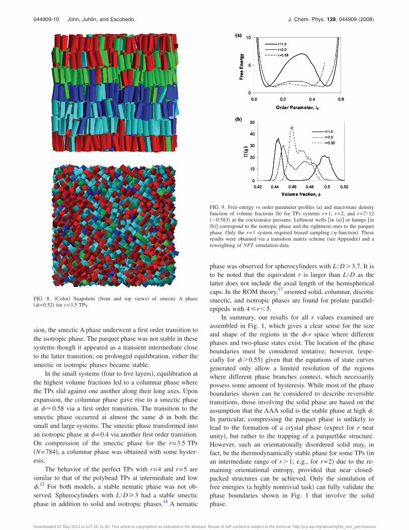
tic” phase�, even though both phases have structures whereparticles form layers with the particle long axes �Z axis�perpendicular to the layer planes, and with particles within agiven layer having little translational order �i.e., a relativelyflat particle distribution function along the X and Y direc-tions�. The key difference between the smectic� phase andthe smectic A phase is that, in the latter, particles within alayer have greater rotational disorder �around the particlelong axes�; i.e., the nematic order parameter for the particleshort axes is less than that for well aligned systems�P2�0.9�. For the systems under consideration, a smectic�to smectic A phase transition is detected upon expansionwhere a slight discontinuity is observed in the equation ofstate. The smectic A phase was stable in a small range of �and upon expansion formed a parquet phase en route to theisotropic phase which formed at ��0.43. The range of �over which the parquet phase was stable appeared to be verynarrow for r=3.0 and 3.2; no parquet phase was observed forr�3.5.

The smaller system simulated for r=3.2 exhibited co-lumnar, smectic A, parquet, and isotropic phases. Thecolumnar-smectic phase transition occurred at similar condi-tions where the solid-smectic transition observed in the largesystem, while the smectic-parquet and parquet-isotropicphase transitions occurred at similar � in both small andlarge systems.

When the r=3 system was simulated with a columnarphase as the starting configuration at close packing, it re-mained stable at high � for the simulation periods we moni-tored but transitioned to the ordered solid as the � ap-proached the smectic phase boundary. This high-� behaviormay be due to ergodic trapping or the high similarity be-tween the free energies of columnar and solid phases. Com-pression from the smectic phase also gave rise to the orderedsolid phase for the r=3 system.

For the r=3 polybead TPs of Ref. 12, the results wereobtained from the expansion of a dense columnar phase�with N=576� and no transition to a solid phase was ob-served. As for the 1�r�2.75 polybead TPs results dis-cussed before, it is likely that the choices of starting configu-ration and of small system size led to biased results. Theser=3 polybead TPs, however, did form a parquet phase thatwas stable in a very narrow region of � and became isotropicfor ��0.486.

Spherocylinders with L /D�3 had a stable smecticphase in addition to solid and isotropic phases.14 In the re-stricted orientation model for parallelepipeds17 with r=2.95,the plastic solid at higher densities undergoes a weak firstorder transition to the discotic smectic phase, which in turnat higher pressures forms a columnar phase. The discoticsmectic phase is a layered phase with the long axes of theparticles lying within the layers and lacks orientational orderin the layers. In the ROM theory, a smectic phase is observedonly for r�6.

3.5ÏrÏ5The system was expanded from an AAA crystal phase.

Systems with six particle layers were studied; i.e., N=2646for r=3.5, N=2400 for r=4.0, and N=2400 for r=5.0 �non-

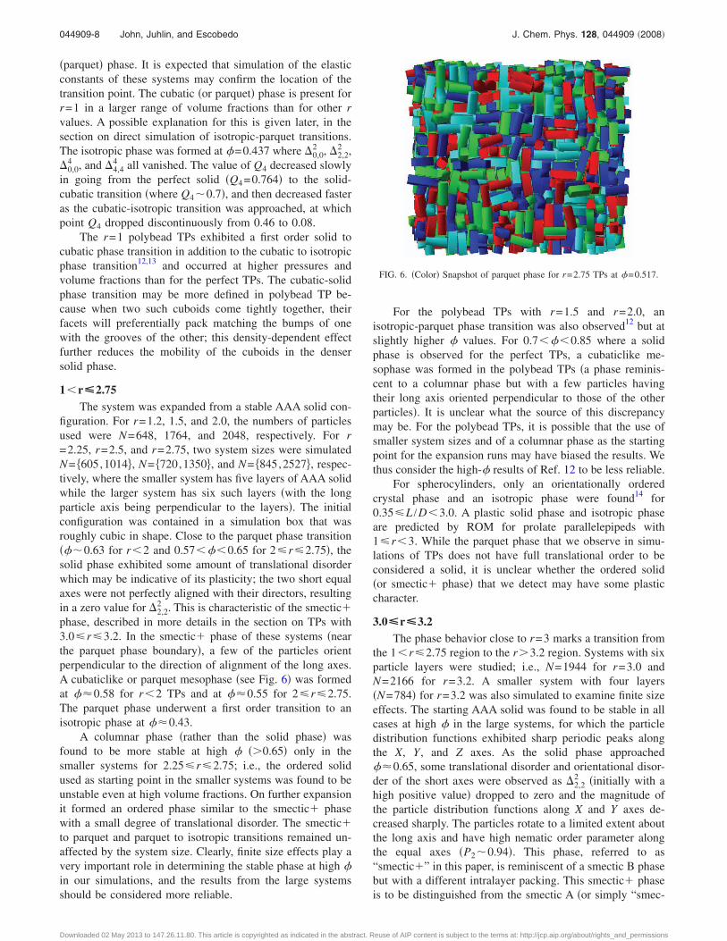
cubic box shapes were used for the latter two systems�.Smaller systems with four layers �N=784� for r=3.5 and fivelayers �N=2000� for r=4.0 were also simulated to examinefinite size effects. The ordered solid phase remained stable inall the large systems. As for the r=3–3.2 systems, the solidphase disorders at �=0.67 by losing first some orientationalorder of the short axes ��2,2

2 becomes zero� and then transla-tional order within layers �see Fig. 7�, to form a smectic�phase, and then completely losing orientational order alongthe TPs’ short axes �see Fig. 8�, to form a smectic A phase. Infact, the equation of state curves revealed a small break asthe smectic� phase �with particle distribution functionsshowing periodic though small peaks along the X and Y axescorresponding to the short particle axes� loses translationalorder �where particle distribution functions along X and Ydirections hover close to 1�. The smectic� phase was stableapproximately in the region 0.56��0.66 with the smecticA phase ensuing at lower concentrations. On further expan-

FIG. 7. �Color� Snapshots �front and top views� of the smectic� phase��0.57� for the r=5 TPs showing the significant lateral translationaldisorder.



sion, the smectic A phase underwent a first order transition tothe isotropic phase. The parquet phase was not stable in thesesystems though it appeared as a transient intermediate closeto the latter transition; on prolonged equilibration, either thesmectic or isotropic phases became stable.

In the small systems �four to five layers�, equilibration atthe highest volume fractions led to a columnar phase wherethe TPs slid against one another along their long axes. Uponexpansion, the columnar phase gave rise to a smectic phaseat ��0.58 via a first order transition. The transition to thesmectic phase occurred at almost the same � in both thesmall and large systems. The smectic phase transformed intoan isotropic phase at �=0.4 via another first order transition.On compression of the smectic phase for the r=3.5 TPs�N=784�, a columnar phase was obtained with some hyster-esis.

The behavior of the perfect TPs with r=4 and r=5 aresimilar to that of the polybead TPs at intermediate and low�.12 For both models, a stable nematic phase was not ob-served. Spherocylinders with L /D�3 had a stable smecticphase in addition to solid and isotropic phases.14 A nematic

phase was observed for spherocylinders with L /D�3.7. It isto be noted that the equivalent r is larger than L /D as thelatter does not include the axial length of the hemisphericalcaps. In the ROM theory,17 oriented solid, columnar, discoticsmectic, and isotropic phases are found for prolate parallel-epipeds with 4�r�5.

In summary, our results for all r values examined areassembled in Fig. 1, which gives a clear sense for the sizeand shape of the regions in the �-r space where differentphases and two-phase states exist. The location of the phaseboundaries must be considered tentative; however, �espe-cially for ��0.55� given that the equations of state curvesgenerated only allow a limited resolution of the regionswhere different phase branches connect, which necessarilypossess some amount of hysteresis. While most of the phaseboundaries shown can be considered to describe reversibletransitions, those involving the solid phase are based on theassumption that the AAA solid is the stable phase at high �.In particular, compressing the parquet phase is unlikely tolead to the formation of a crystal phase �expect for r nearunity�, but rather to the trapping of a parquetlike structure.However, such an orientationally disordered solid may, infact, be the thermodynamically stable phase for some TPs �inan intermediate range of r�1; e.g., for r=2� due to the re-maining orientational entropy, provided that near closed-packed structures can be achieved. Only the simulation offree energies �a highly nontrivial task� can fully validate thephase boundaries shown in Fig. 1 that involve the solidphase.

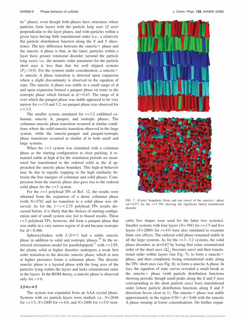
FIG. 9. Free-energy vs order parameter profiles �a� and macrostate densityfunction of volume fractions �b� for TPs systems r=1, r=2, and r=7 /12��0.583� at the coexistence pressure. Leftmost wells �in �a�� or humps �in�b�� correspond to the isotropic phase and the rightmost ones to the parquetphase. Only the r=1 system required biased sampling �� function�. Theseresults were obtained via a transition matrix scheme �see Appendix� and areweighting of NPT simulation data.

FIG. 8. �Color� Snapshots �front and top views� of smectic A phase��=0.52� for r=3.5 TPs.



Direct simulations of isotropic-parquet transitions

The isotropic-parquet phase transitions occur for systemswith r values ranging from 0.54 to slightly above r=3.2.Figure 9 shows �a� representative free-energy profiles�effectively—ln ��I4�� as a function of I4, and �b� the prob-ability density �histograms� of volume fractions �� at theisotropic-parquet coexistence pressure. For r=0.583�=7 /12�, 1, and 2, the coexistence pressures �found fromhistogram reweighting from simulations conducted at nearbypressures� were 11.74, 6.01, and 3.365, while the number ofparticles were 588, 512, and, 500, respectively. A distinctivefeature of the transition for r=1 is that the free-energy bar-rier between phases �on the macrostate space of either I4 orvolume fraction� is much larger than for other r values.In fact, a relatively flat isotropic-parquet free-energy profileis also evidenced for other r values not too far from 1�e.g., r=0.8 and 1.2, results not shown�. This characteristicseems to underline the fact that the r=1 parquet phase or“cubatic” phase is special amongst the other parquet cases. Infact, 90° particle rotations around any of the three orthogonalcubatic directors leave the r=1 system unchanged while thisrotational symmetry is broken when r�1. In a sense, ther=1 parquet phase is more ordered and farther away fromthe isotropic phase than the parquet phases for r�1 systems.

The small free-energy barrier and the blurring betweenthe concentrations of the isotropic and parquet phases for

r�1 systems bring up the question of the “order” of thetransition and the possibility of systems with vanishing inter-facial free energy. However, even when the two histogrampeaks merge into a broad mesa �like in Fig. 9�, it is stillpossible to approximately deconvolute it into two quasi-Gaussians whose means would allow us to get two distinctcoexistence concentrations corresponding to the two phases;such a discontinuous change in concentration �volume� is thesignature of a first order transition. To examine the role offinite size effects in our results, we used larger boxes forselected cases. Figure 10 shows concentration histograms forr=1.5 using 486 and 1152 particles. Our observations for thissystem that can be generalized to other r�1 systems aresummarized as follows:

�1� A larger system tends to produce narrower concentra-tion �or volume� histograms with a more pronouncedtwo-peak structure. The estimated interfacial free en-ergy and the coexistence pressure both grow with sys-tem size.

�2� The location of the two peaks in concentration in the�� histogram does not shift significantly with systemsize; however, the positions of the minima in I4 in thefree-energy landscape tend to shift toward smaller val-ues for larger systems. This can be explained by theobservation that for larger systems, the global orienta-tion of the parquet phase �i.e., the orientation of thephase directors� becomes less correlated with thesimulation-box axes �an effect of the periodic boundaryconditions�.

�3� The use of a bias function ��I4� to force uniform sam-pling over the I4 domain tends to flatten out the inter-facial region; i.e., to lower slightly the free-energy bar-rier. We suspect that this is due to the nonergodicity ofthe sampling of interfacial regions and that the global I4

adopted here is not a very “good” reaction coordinatefor the transition path; the natural hysteresis in goingback and forth between the stable phases is amplifiedby the enhanced interfacial sampling and leads to anartificial smoothing out of the interfacial features. Inthis context, unbiased simulations are preferable �pro-vided that a handful of transitions take place during therun�.

�4� We also measured the relative orientational orderbetween particles as function of their distance d�i.e., I4�d�, results not shown� and confirmed that after ashort decay for 1�d�2, it reaches a plateau for longerd values �I4�0.39 for the r=1.5, N=1152 system�,consistent with the idea of long range order.

The remark �3� above on ergodicity issues may seem contra-dictory to the relatively small free-energy barrier betweenphases. Our observations indicate, however, that the apparent“kinetics” of phase interconversion is rather slow. This sug-gests that in configurational space, the free-energy barrier isdiffusive; i.e., in the transition region the system encountersshallow but very numerous traps.

FIG. 10. Isotropic-parquet coexistence free-energy vs order parameter �a�and macrostate density function of volume fractions �b� for TP systems withr=1.5. Leftmost wells �in �a�� or humps �in �b�� correspond to the isotropicphase and the rightmost ones to the parquet phase. N is the number ofparticles in the box. The results in �b� correspond to unbiased simulationruns and the P values shown are the coexistence pressures estimated byreweighting. All results were obtained via a transition matrix treatment ofNPT ensemble data �see Appendix�.



IV. CONCLUSIONS

The phase diagram for perfect freely rotating hard TPswas mapped out and compared with existing results for re-lated models. A very rich phase diagram was obtained for0.125�r�5. A discotic smectic phase, which is predictedby the restricted orientations model �ROM� theory, was notobtained in our simulations. The presence of the parquetphase, not predicted by the ROM theory, is confirmedthrough our simulations that account for the rotational free-dom and smooth surfaces of the parallelepipeds. The parquetphase seems to be the last step in the transition path from theordered phase region to the isotropic phase except for veryoblate �r�0.54� and very prolate �r�3.2� systems. The dis-ordering of the more ordered phase occurs by gradual loss oftranslational order and stepwise changes in particle orienta-tion: in the parquet phase the preferential orientation of thelong or short axes is lost so that all particle axes becomeperpendicular to one another. The smectic� phase shows upas a transitional state where the solid phase first gains a littleorientational and translational entropy en route to formingmesophases with more orientational entropy.

Our results for low and intermediate volume fractionsare similar to those of our earlier simulations12 using TPsapproximated by polybead models. In general, the volumefractions at which phase transitions occurred for the poly-bead TPs were different from those for the perfect TPs; e.g.,disordering tended to occur at higher � in the polybeadmodel. This can be explained by considering that the poly-bead TPs, being more rounded, tend to rotate more easily anddisorder more readily. It is expected that the polybead behav-ior will approach that of the perfect TPs as the shape reso-lution increases �i.e., as more numerous “small” beads areused to represent a given TP�. Overall, the polybead modelwas effective in predicting the rough features of the perfectTP phase diagram for low and intermediate volume fractions.Reliable phase predictions at higher volume fractions requirethe use of large N to eliminate system size effects. However,large enough systems were not used for the polybead-TPstudy, a task that would have required very long simulationtimes.

The multicanonical simulations provided more insightinto the isotropic-parquet phase transitions �which occur for0.54�r�3.2�. In particular, they showed that the free-energy barrier was the highest for the r=1 system, that theinterfacial free energy and coexistence pressure increase withsystem size, and that the global orientation of the parquetphase became less correlated with the simulation box axes inlarge systems. A more detailed analysis is also needed for thephase transitions occurring at higher volume fractions; e.g.,to unambiguously identify the character of the solid phaseand to pinpoint the transition between this phase and theliquid crystal phase that forms �at a given r� upon decreasing�.

In the TPs studied here, the geometry of the particlesdetermines their preferential local packing which ultimatelyleads to their entropic self-assembly into phases having vary-ing degrees of translational and orientational orders. Differ-ent phases maximize their entropy via different contribu-

tions; e.g., the columnar and solid phases have littleorientational entropy, but the columnar phase has large trans-lational entropy along one of the particle axes while the crys-tal only allows a little translational entropy via local vibra-tions. While it is easy to see that the layering in a smecticphase implies less translational entropy than in a nematicphase �though both have similar orientational entropy�, it ismore difficult to rank the order of the parquet phase relativeto the smectic phase, given that they realize translational andorientational entropies in very different ways. The ability totune particle geometry �like the aspect ratio in TPs� to pro-mote the formation of a useful structure is clearly of practicalinterest and the knowledge of the phase diagram should pro-vide guidance to experimentalists attempting to engineersuch colloidal systems. The optical properties of the as-sembled mesophases of sharp-faceted colloids may havepromising applications in photonics, sensing, and imaging.The effect of gravity and confinement on mesophase forma-tion should also be investigated given that most experimentalrealizations of colloidal suspensions of TPs do not involvedensity-matched solvent-particle systems and sedimentationon a surface occurs. Some of the mesophases encounteredmay also have interesting rheological properties such asyield-stress behavior and shear thickening, which couldmake them appealing to novel applications; exploratorysimulations of these properties are currently under way.

ACKNOWLEDGMENTS

The authors acknowledge financial support from NSF�Grant No. 0553719� and ACS-PRF. The authors are gratefulto Professor K. Bala �Cornell University� for directing themto the concept of Oriented Bounding Boxes and to ProfessorCharlles Abreu �U. Campinas� for help with visualizationsoftware, and to a reviewer of this paper for pointing them tothe use of the Dm,n

l order parameters.

APPENDIX: CALCULATION OF MACROSTATEPROBABILITIES

Since we use the isothermal-isobaric ensemble for allsimulation reported in this work, in most of the equationsand functions that follow, the constancy of N and T is im-plicit. The pressure at which the original simulation is per-formed is denoted as P0. The macrostate probabilities � andfree-energy functions associated to isotropic-parquet phasetransitions can be estimated from the “multicanonical”�-biased runs alluded to in Sec. II by using either histogramreweighting or a transition matrix approach as explained be-low. In the simulations described in the text, � was only afunction of � and was found iteratively by trying to achieveuniform sampling of the � domain; i.e., by using �� ln �� P0�+constant, where � corresponds to the mostrecent estimation of the macrostate probabilities �found fromeither the collected � histogram or the transition matrixmethod�. For generality, it is assumed below that � is anarbitrary function that depends on both V and �; i.e., �=��V ,��.



Visited states approach: Histogram reweighting

Assuming that the biasing weight function ��V ,�� hasremained fixed throughout, one can measure during a simu-lation the “biased” probability distribution of �V ,�� mac-rostates �accumulated as a simple list� ��V ,� N , P0 ,T ,�� tobe written as ��V ,� P0 ,�� by keeping the T, N dependenceimplicit. The unbiased macrostate probability can be foundfrom

��V,�P0� � ��V,�P0,��exp��V,�� , �A1�

and reweighting to a different pressure P can be achieved byusing

��V,�P� � ��V,�P0,��exp��V,�� − �V�P − P0�� .

�A2�

From this, marginal probabilities of volume or order param-eter macrostates can be easily found by integration; e.g.,from

��VP� � �I

��V,�IP0,��exp��V,�I� − �V�P − P0�� ,

�A3�

��P� � �I

��VI,�P0,��exp��VI,�� − �VI�P − P0�� .

�A4�

One can use Eq. �A3�, for example, to find coexistence con-ditions for two phases sampled during the simulation. Forthis purpose, one finds a P value for which a bimodal��V P� versus V function occurs having equal areas undereach of the peaks �each peak represents one phase�. Althoughnot implemented here, if ��V ,�� has changed during a run�due to successive iterations to refine it�, it is possible to usea multihistogram reweighting approach to extract ��V ,� P�,as described in Ref. 29.

Transition matrix approach

The basis for this method and its connection toacceptance-ratio methods has been explained in detail in Ref.30. Here we simply apply Eq. �9� from Ref. 30 to our spe-cific situation to connect macrostate probability ratios totransition probabilities �right hand side� measured during thesimulation:

��VK,�L��VI,�J�

=�I,JPacc�VI,�J → VK,�L�/nI,J

�K,LPacc�VK,�L → VI,�J�/nK,L, �A5�

where Pacc are the acceptance probabilities �e.g., Eq. �2�� ofthe indicated transitions and nI,J are the number of times thatthe system, being in the macrostate denoted by the labels�I ,J� attempted a transition that could result in a macrostatechange. In Eq. �A5� the �’s can refer to the macrostate prob-abilities biased with � or unbiased. In the former case,

��VI,�JP0,�� = ��i,j�I,J

p�i, j�

= ��i,j�I

exp�− ��VI,�J� − �P0VI − �U��i,j��

= exp�− ��VI,�J� − �P0VI�q�N,T,VI,�J� .

�A6�

Equation �A6� defines the function q which is a “local” ca-nonical partition function wherein the sum of microstates isrestricted to those having a specific value of �. Once ratiosof the � functions have been found using Eq. �A5�, one canfind q values using Eq. �A6�. The canonical partition func-tion corresponding to the fixed values of N ,T, and any par-ticular V is simply:

Q�N,T,VI� = �all K

q�N,T,VI,�K� , �A7�

thus

Q�N,T,VI� � exp��P0VI��K

exp��VI,�K��

��VI,�KP0,�� . �A8�

Since the arbitrary weight function ��V ,�� does not bias thesampling of microstates within any particular bin �VI ,�J�,one can accumulate statistics for the unbiased transitions inboth � and Pacc, so that

��VI,�JP0� = ��i,j�I,J

p�i, j� � ��i,j�I,J

exp�− �P0VI − �U��i,j��

= exp�− �P0VI� ��i,j�I,J

exp�− �U��i,j��

= exp�− �P0VI�q�N,T,VI,�J� , �A9�

Q�N,T,VI� � exp��P0VI��K

��VI,�KP0� . �A10�

The unnormalized probability of different volume mac-rostates for a given pressure P is then

��VIP� � Q�N,T,VI�exp�− �PVI� . �A11�

The unnormalized probability of different order-parametermacrostates is given by

��JP� � �I

q�N,T,VI,�J�exp�− �PVI�

= �I

��VI,�JP0�exp�− ��P − P0�VI� . �A12�

Of course, Eqs. �A11� and �A12� achieve essentially thesame as Eqs. �A3� and �A4�, respectively �e.g., Eq. �A11� canbe used to find phase coexistence conditions�. The resultsreported in Figs. 9 and 10 correspond to the former equations�which were seen to agree quantitatively with those of thevisited states approach�. The main advantage of the transitionmatrix approach is that ��V ,�� need not be constant duringthe run. In fact, if one stores statistics for the hypotheticalunbiased transitions �without � in the acceptance rule� thenone can obtain unbiased macrostate probability functions



�e.g., Eqs. �A11� and �A12�� even if during the run � wasiteratively changed to improve sampling. This reduces thetotal simulation time needed to get such unbiased � func-tions. However, for several of the TP systems of interest, no� weights were needed and so in those cases the transitionmatrix approach offered no compelling advantage overhistogram reweighting �beyond perhaps slightly better statis-tics�.

Calculation of macrostate probability ratios

Estimation of � ratios from Eq. �A5� is not a trivial tasksince such ratios should be independent on the path taken toachieve a macrostate transition �i.e., via a single step or mul-tiple “smaller” ones�.30 While several approaches can beused to estimate “optimal” ratios, we adopted one that fol-lows closely the ideas presented in Refs. 30 and 31.

Note first that moves that affect V �volume moves� aredecoupled from those that alter � �particle rotation moves�.Further, in practice, only transitions involving changes be-tween �at most� neighboring V values or between neighbor-ing � values occur. If we define aI,J=ln ��VI ,�J P0� we canthen specialize Eq. �A5� for those two cases by defining thefollowing incremental logarithms of � ratios:

�aI,J→I+1,J = ln��VI+1,�JP0��VI,�JP0�

= ln� �I,JPacc�VI → VI+1�/nI,JV

�I+1,JPacc�VI+1 → VI�/nI+1,JV , �A13�

�aI,J→I,J+1 = ln��VI,�J+1P0��VI,�JP0�

= ln� �I,JPacc��J → �J+1�/nI,J�

�I,J+1Pacc��J+1 → �J�/nI,J+1� , �A14�

where nI,J is the total number of times that the system was atmacrostate �VI ,�J� and a move that could alter the super-scripted property �V or �� was attempted. We seek to mini-mize the total variance in the estimation of the aI,J values,

�tot2 = �

J�

I

�aI,J − aI+1,J + �aI,J→I+1,J�2

�I,J→I+1,J2

+ �I

�J

�aI,J − aI,J+1 + �aI,J→I,J+1�2

�I,J→I,J+12 , �A15�

with

�I,J→K,L2 = ��

I,JPacc�VI,�J → VK,�L�−1

+ ��K,L

Pacc�VK,�L → VI,�J�−1. �A16�

By setting d�tot2 /daI,J=0, we get N�M equations of the

form

aI,J

�I,J2 −

aI+1,J

�I,J→I+1,J2 −

aI−1,J

�I−1,J→I,J2 −

aI,J+1

�I,J→I,J+12 −

aI,J−1

�I,J−1→I,J2

= −�aI,J→I+1,J

�I,J→I+1,J2 +

�aI−1,J→I,J

�I−1,J→I,J2 −

�aI,J→I,J+1

�I,J→I,J+12

�+�aI,J−1→I,J

�I,J−1→I,J2 . �A17�

For I=1,2 , . . . ,N and J=1,2 , . . . ,M, where

1

�I,J2 =

1

�I,J→I+1,J2 +

1

�I−1,J→I,J2 +

1

�I,J→I,J+12 +

1

�I,J−1→I,J2 .

�A18�

Solution of this set of linear equations yields “optimal” val-ues for the �unknowns� aI,J.

1 C. J. Murphy, T. K. Sau, A. M. Gole, C. J. Orendorff, J. Gao, L. Gou, S.E. Hunyadi, and T. Li, J. Phys. Chem. B 109, 13857 �2005�.

2 Y. Jun, J. Seo, S. J. Oh, and J. Cheon, Coord. Chem. Rev. 249, 1766�2005�.

3 Z. Pu, M. Cao, J. Yang, K. Huang, and C. Hu, Nanotechnology 17, 799�2006�.

4 B. J. Wiley, Y. Chen, J. M. McLellan, Y. Xiong, Z. Li, D. Ginger, and Y.Xia, Nano Lett. 7, 1032 �2007�.

5 X. Huang, I. H. El-Sayed, W. Qian, and M. A. El-Sayed, J. Am. Chem.Soc. 128, 2115 �2006�.

6 Y. Sun and Y. Xia, Science 298, 2176 �2002�.7 Y. Xiang, X. Wu, D. Liu, X. Jiang, W. Chu, Z. Li, Y. Ma, W. Zhou, andS. Xie, Nano Lett. 6, 2290 �2006�.

8 T. K. Sau and C. J. Murphy, Langmuir 29, 2923 �2005�.9 Y. Sun, L. Zhang, H. Zhou, Y. Zhu, E. Sutter, Y. Ji, M. H. Rafailovich,and J. C. Solokov, Chem. Mater. 19, 2065 �2007�.

10 X. Zhang, D. Zhang, X. Ni, and H. Zheng, Chem. Lett. 35, 1142 �2006�.11 Z. T. Deng, F. Q. Tang, D. Chen, X. W. Meng, L. Cao, and B. S. Zou, J.

Phys. Chem. B 110, 18225 �2006�.12 B. S. John and F. A. Escobedo, J. Phys. Chem. B 109, 23008 �2005�.13 B. S. John, A. Stroock, and F. A. Escobedo, J. Chem. Phys. 120, 9383

�2004�.14 P. Bolhuis and D. Frenkel, J. Chem. Phys. 106, 666 �1997�.15 J. A. C. Veerman and D. Frenkel, Phys. Rev. A 45, 5632 �1992�.16 M. A. Bates and D. Frenkel, Phys. Rev. E 57, 4824 �1998�.17 Y. Martinez-Raton, Phys. Rev. E 69, 061712 �2004�.18 A. Casey and P. Harrowell, J. Chem. Phys. 103, 6143 �1995�.19 S. Gottschalk, M. C. Lin, and D. Manocha, Comput. Graph. 30, 171

�1996�.20 R. Blaak, D. Frenkel, and B. M. Mulder, J. Chem. Phys. 110, 11652

�1999�.21 P. J. Steinhardt, D. R. Nelson, and M. Ronchetti, Phys. Rev. B 28, 784

�1983�.22 C. Zannoni, The Molecular Physics of Liquid Crystals, edited by G. R.

Luckhurst and G. W. Gray �Academic, New York, 1979�, pp. 51–83.23 R. Blaak and B. Mulder, Phys. Rev. E 58, 5873 �1998�.24 D. M. Brink and G. R. Satchler, Angular Momentum, 2nd ed. �Oxford

University Press, Oxford, 1968�.25 J. P. Straley, Phys. Rev. A 10, 1881 �1974�.26 D. Frenkel and B. Smit, Understanding Molecular Simulation: From Al-

gorithms to Applications, 2nd ed. �Academic, New York, 2002�.27 I. Gospodinov and F. A. Escobedo, J. Chem. Phys. 122, 164103 �2005�.28 See EPAPS Document No. E-JCPSA6-127-003748 for tables containing

the order parameters P2, P4 near phase transitions for the TPs. This docu-ment can be reached through a direct link in the online article’s HTMLreference section or via the EPAPS homepage �http://www.aip.org/pubservs/epaps.html�.

29 C. R. A. Abreu and F. A. Escobedo, J. Chem. Phys. 124, 054116 �2006�.30 F. A. Escobedo and C. R. A. Abreu, J. Chem. Phys. 124, 104110 �2006�.31 F. A. Escobedo, Phys. Rev. E 73, 056701 �2006�.



Documents

Phase behavior of colloidal hard perfect tetragonal parallelepipeds