Phase Behavior and Reliable Computation of

High Pressure Solid-Fluid Equilibrium with Cosolvents

Aaron M. Scurto†, Gang Xu‡, Joan F. Brennecke* and Mark A. Stadtherr

Department of Chemical and Biomolecular Engineering

University of Notre Dame

182 Fitzpatrick Hall

Notre Dame, IN 46556

USA

†Current Address: Institut für Technische Chemie und Makromolekulare Chemie, RWTH-Aachen, Worringerweg 1, Aachen, D-52074, Germany ‡Current Address: SimSci-Esscor/Invensys, 26561 Rancho Parkway South, Suite 100, Lake Forest, CA 92630 *Author to whom correspondence should be addressed: Tel.: (574) 631-5847, Fax: (574) 631-8366, E-mail: jfb@nd.edu

(February 2003)

(revised, June 2003)

2

Abstract

The identification of the correct, stable solution to a phase equilibrium problem,

given a particular thermodynamic model, is essential for the design of separation processes.

It is also important in the selection of an appropriate model to represent experimental data.

The need for a completely reliable method to test for phase stability is particularly pressing

when the number of phases likely to be present is not intuitive to the user, as is frequently

the case with high-pressure systems. Previously, we have a presented a completely reliable

computational technique, based on interval analysis, to correctly identify phase equilibrium

and test for phase stability in binary solvent-solute systems, that include the possibility of a

solid phase, using any of a variety of cubic equations of state as the thermodynamic model.

Here we extend the methodology to include multicomponent solvent-solute-cosolvent

systems where the likelihood of additional phase formation is even greater than in the

binary case. Gaseous or liquid cosolvents are frequently used in supercritical fluid

extraction processes, and are integral in processes such as the gas anti-solvent process

(GAS) to precipitate uniform solid particles. Using several examples from the literature, we

demonstrate how the new computational technique can be used to identify experimental

data that may have been misinterpreted and to identify models that do not predict what the

modeler intended.

Keywords: Solid-Fluid Equilibrium, Supercritical Fluids, Phase Stability, Phase

Equilibrium, Interval Analysis

3

1. INTRODUCTION

The calculation of solid-fluid equilibrium using an equation of state has formed the

foundation for the design of supercritical fluid extraction processes.1 It is also important in

designing solid precipitation processes using high-pressure gases, such as the rapid expansion of

a supercritical solution (RESS), gas anti-solvent (GAS) and supercritical anti-solvent (SAS)

processes.2,3,4,5,6 In a previous paper7 we presented a framework for the completely reliable

computation of solid-fluid equilibrium, using interval analysis to solve correctly the phase

equilibrium and phase stability problems, when a cubic equation of state is used as the

thermodynamic model for binary solvent-solute systems. We chose to apply the technique using

cubic equations of state because they are simple, generally give good representations of high-

pressure phase behavior, and are used extensively in industry. In this paper we extend this

framework for the reliable computation of solid-fluid equilibrium to multicomponent solvent-

solute-cosolvent mixtures.

The correct solution of multicomponent high-pressure phase equilibrium problems

involving solids is vitally important to process design and to the evaluation of model

performance. Without the identification of the correct, thermodynamically stable solutions to a

model, experimental data can be misinterpreted and gross design errors can be made. For

instance, we have shown7 that for binary systems in the literature, there are instances where data

is reported as solid-fluid equilibrium but the equation-of-state model, with parameters regressed

by the authors from their experimental data, actually predicts vapor-liquid equilibrium (VLE).

This generally occurs because the researchers assume that the model will predict solid-fluid

equilibrium and either do not check for phase stability or do the phase stability check using a

local solution technique that does not guarantee the correct solution. In some cases, authors have

4

recognized that their experimental data seemed suspicious (i.e., solubilities too high for the solid

dissolved in a supercritical fluid phase) and they later verified that what they had originally

believed to be solid-fluid equilibrium was really vapor-liquid equilibrium, in agreement with the

model predictions.8,9 As we will discuss here, the likelihood of such errors greatly increases

when one computes high-pressure phase equilibria involving solids in multicomponent mixtures

using conventional numerical solution techniques.

There are a wide variety of industrial processes where correct modeling of solid-fluid

equilibrium is important. The most obvious are those involving supercritical fluid extraction,

which has found extensive application for coffee and tea decaffeination, and for the recovery of

components in natural products, such as hops, essential oils and nutraceuticals.1 A common

practice is to add a chemical modifier (called a cosolvent or entrainer) to the supercritical fluid in

order to increase solute solubility or selectivity. For instance, a polar cosolvent such as ethanol

might be added to nonpolar supercritical CO2 to increase the solubility of polar compounds. As

a result, most supercritical fluid extractions involve multicomponent mixtures. Moreover, there

is a large body of data in the literature on the solubility of solid solutes in supercritical fluids that

have been modified with the addition of either gaseous or liquid cosolvents.10,11,12,13 In

particular, the practice of adding cosolvents has been used extensively with supercritical carbon

dioxide, which has a relatively low solvent power, but which is used frequently since it is

inexpensive and environmentally benign. A supercritical extraction process with a cosolvent

usually begins by first mixing a certain proportion of the cosolvent and solvent at a particular

temperature and pressure that ensures that a single phase exists, i.e., above the mixture critical

point of the binary solvent-cosolvent system. Then this mixture is passed to another unit to

contact the solid and extract the solute. In modeling the solubility of the solute in the extraction,

5

the solvent to cosolvent ratio is fixed, and then one solves for the solubility that satisfies the

equifugacity requirement of the solute in both the solid and supercritical phases. It is customary

to neglect the possibility of a second fluid phase (liquid) forming (fluid phase instability) in both

measurement and modeling as long as the original solvent-cosolvent mixture remains above its

binary mixture critical point. However, as we will demonstrate here, this can lead to erroneous

results.

A second type of application in which reliable modeling of high-pressure,

multicomponent phase behavior involving a solid phase is important is materials production

using the RESS, GAS or SAS processes. For instance, the point at which a solid precipitates

from a liquid with the addition of a pressurized gas forms the basis of the gas anti-solvent

process (GAS) and supercritical anti-solvent process (SAS). Therefore, these processes

invariably require knowledge of the multicomponent saturation conditions for adequate

development. A third type of application of interest in this context is the use of supercritical

fluids as solvents for reactions. Many reactions in supercritical fluids involve the presence of

both solid and liquid reactants, products, and catalysts, and reliable computation of phase

behavior is important because frequently single phase operation is desired. For a review of

homogeneous reactions in supercritical fluids see Jessop et al.14

We will present here a completely reliable computational strategy, based on interval

analysis, to find the solution to high-pressure, multicomponent phase equilibrium problems

involving a solid phase. The examples given are for solid-fluid equilibrium in the presence of

cosolvents, as might be encountered in a supercritical fluid extraction process, but this

computational technique can also easily be used in modeling the phase behavior in the other

high-pressure phase equilibrium applications mentioned above. First, we will present a brief

6

overview of the features of high-pressure solid-fluid phase behavior, in order to illustrate the

inherent complexity that can be encountered in modeling these systems. Then we will detail the

problem formulation and summarize the solution method based on interval analysis. Finally, we

will give several examples in which we have applied this technique. These are taken from the

literature, and illustrate the importance of reliable computation of high-pressure phase

equilibrium for multicomponent mixtures with solids present.

2. BACKGROUND

In this section, we will present a brief overview of the features of high-pressure solid-

fluid phase behavior, and discuss some of the modeling difficulties that can result.

2.1 Binary Phase Behavior

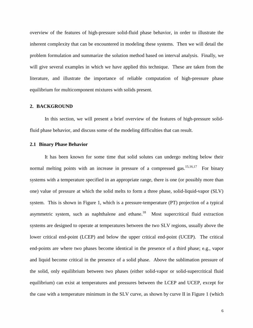
It has been known for some time that solid solutes can undergo melting below their

normal melting points with an increase in pressure of a compressed gas.15,16,17 For binary

systems with a temperature specified in an appropriate range, there is one (or possibly more than

one) value of pressure at which the solid melts to form a three phase, solid-liquid-vapor (SLV)

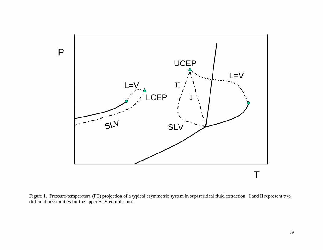
system. This is shown in Figure 1, which is a pressure-temperature (PT) projection of a typical

asymmetric system, such as naphthalene and ethane.18 Most supercritical fluid extraction

systems are designed to operate at temperatures between the two SLV regions, usually above the

lower critical end-point (LCEP) and below the upper critical end-point (UCEP). The critical

end-points are where two phases become identical in the presence of a third phase; e.g., vapor

and liquid become critical in the presence of a solid phase. Above the sublimation pressure of

the solid, only equilibrium between two phases (either solid-vapor or solid-supercritical fluid

equilibrium) can exist at temperatures and pressures between the LCEP and UCEP, except for

the case with a temperature minimum in the SLV curve, as shown by curve II in Figure 1 (which

7

will be discussed below). At temperatures close to the UCEP or LCEP one can observe large

changes in solvent power with small changes in pressure.19 If the temperature is above the

UCEP (or above the minimum in the SLV curve, as discussed below), the solid will melt and one

will observe VLE, unless a large loading of the solid solute is used, which will result in solid-

liquid equilibrium (SLE). If the pressure is further increased, the liquid and vapor phases will

disappear at the mixture critical point and either a single phase will exist or one will observe SFE

at large solute loadings. The upper (higher temperature) SLV line emanates from the solute

triple point and proceeds directly to the UCEP as illustrated as SLV curve I in Figure 1.

However, for some systems, e.g. naphthalene and CO2,9 and biphenyl and CO2,

9 the SLV line

proceeds through a minimum in temperature (SLV curve II in Figure 1) before reaching the

UCEP. For these systems, simply remaining below the UCEP temperature does not guarantee

working in a SFE region; one must be below the minimum in the SLV curve.

Cubic equations of state (EOS) can describe all of the types of phase behavior mentioned

above. However, we have shown previously that there can exist multiple solubility roots to the

equifugacity equations for solid-fluid equilibrium when using cubic EOS at temperatures near

the SLV lines.7 The key to identifying the correct root(s), and, thus, the correct type of phase

equilibrium (SFE, SLE or SLV), is testing the roots for thermodynamic stability. If there is no

solubility root that is both stable and feasible (based on overall solute loading and material

balance), then there is no solid phase present at equilibrium, and a multiphase flash calculation

can be done to determine the number and composition of fluid phases present. Xu et al.7

demonstrate that their solution strategy can correctly deal with all these cases, thus determining

the correct behavior. This is extremely useful in modeling experimental data to ensure that one

does not regress parameters that predict the existence of phases that are not observed

8

experimentally. This is also important in alerting experimentalists a priori to the possibility of

unanticipated phase transitions. Obviously, a priori predictions are only as good as the models

(and interaction parameters) employed, but they can at least qualitatively indicate the phase

behavior to be expected. Whether one assumes SFE, or includes the possible existence of liquid

phases,20,21,22 and whether there are single or multiple roots to the equifugacity equation, the key

step in computing the correct phase behavior is performing a completely reliable phase stability

test. This is all the more important for the high-pressure multicomponent case, as discussed next.

2.2 Ternary Phase Behavior

In ternary mixtures, as occurs when a cosolvent is added to a supercritical fluid to

enhance the solubility or selectivity of a solid solute, the possibility of liquid phase formation is

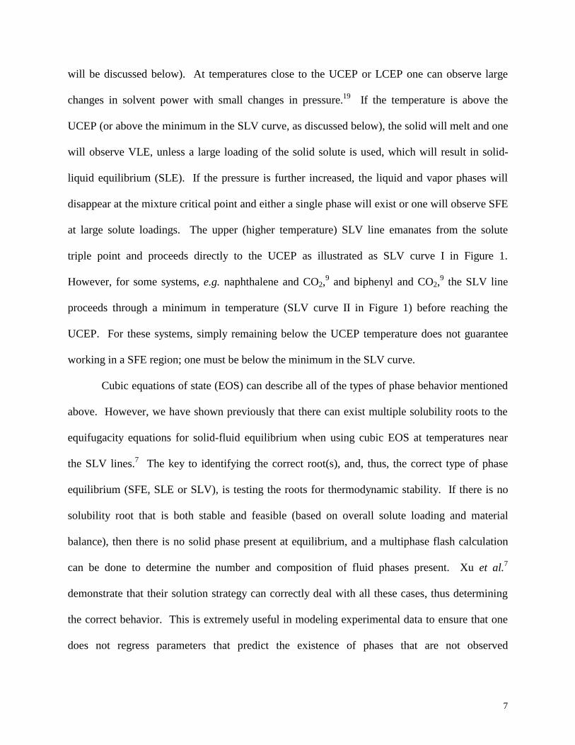
greatly enhanced in comparison to the binary case. According to the Gibbs phase rule, a third

component extends SLV equilibrium from a line to a region of pressure and solubility at a given

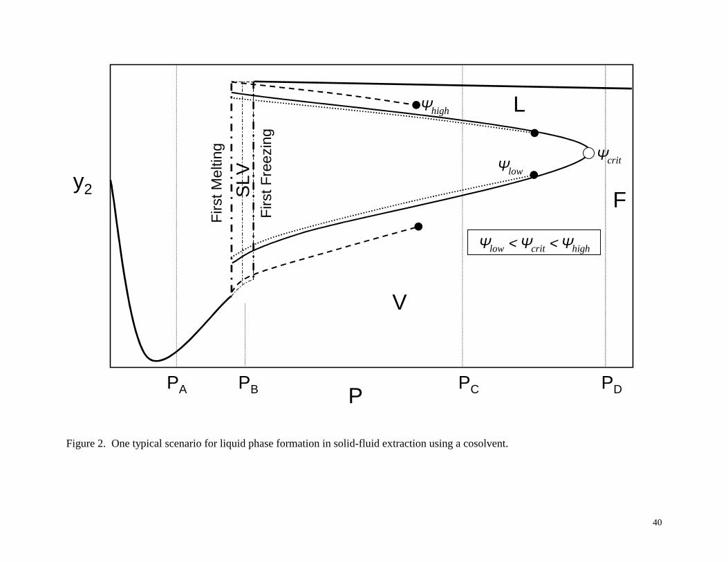
temperature. This is represented in Figure 2, which shows a typical scenario encountered when a

gaseous or liquid cosolvent is added to a supercritical fluid at a certain initial concentration. At

low pressures, PA in Figure 2, solid-vapor (SVE) equilibrium exists, with the solute solubility

(mole fraction) y2 in the vapor shown by the solid curve, assuming an overall solute loading of at

least y2 (otherwise there will be a single vapor phase mixture). As pressure is increased, the SLV

region is encountered, bounded at its lowest pressure by the first melting line, and at its highest

pressure by the first freezing line. In this region, PB in Figure 2, if there is a sufficiently large

solute loading, then there is SLV equilibrium. At lower solute loadings, VLE would exist, and at

still lower solute loadings, a single vapor phase mixture would exist. If the solute loading is such

that VLE occurs, then the compositions of the liquid and vapor phases depend on the loading.

This is shown in the figure by the three different curves at low, “critical” and high loadings, ψlow

9

< ψcrit < ψhigh. Only at one particular loading, designated ψcrit, does the curve close at higher

pressure. At the other loadings, the overall mixture composition point is simply no longer in the

VLE region as the pressure is increased (note that Figure 2 is a two-dimensional representation

of a three component system). Beyond the SLV region, PC in Figure 2, one can observe SLE,

single-phase liquid, VLE, or single-phase vapor, depending on the solute loading. If SLE exists

(high solute loading) then the liquid phase composition (solute solubility) is given by the solid

line at high mole fraction. At high pressures, PD in Figure 2, SLE exists for high solid loadings;

at lower loadings one would observe a single fluid phase.

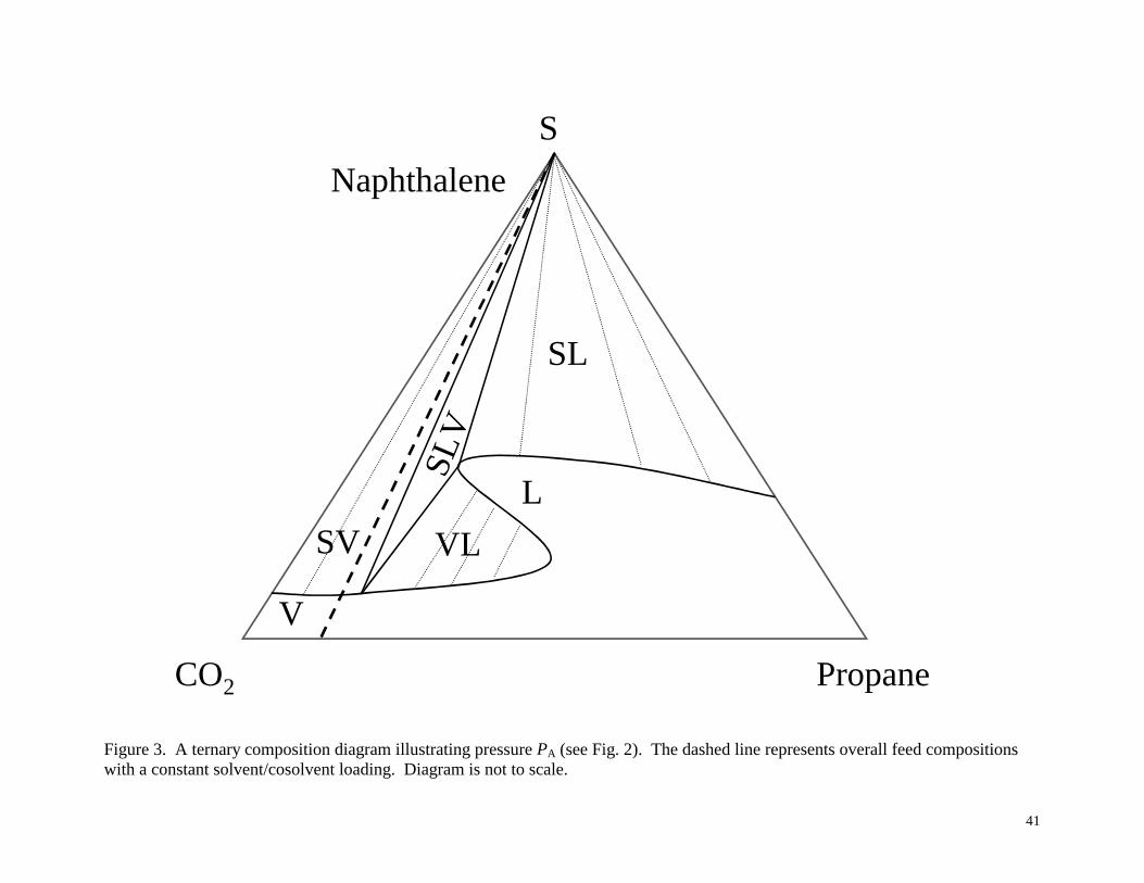
The phase behavior explained above can be further visualized using the triangular ternary

phase diagrams in Figures 3-6, corresponding to the pressures PA, PB, PC and PD shown

schematically in Figure 2. Although certainly not to scale, the reader might think of the system

as being naphthalene (solute) and CO2 (solvent), where propane has been added as a cosolvent.

On each plot, there is a dashed straight line that extends from the pure naphthalene vertex to the

CO2/propane edge of the triangle. This line represents a constant solvent/cosolvent loading, as

one would encounter with a premixed CO2/propane mixture, such as that used by Smith and

Wormald.18 The position of the initial overall composition point along that straight line depends

on how much solute (naphthalene) is loaded.

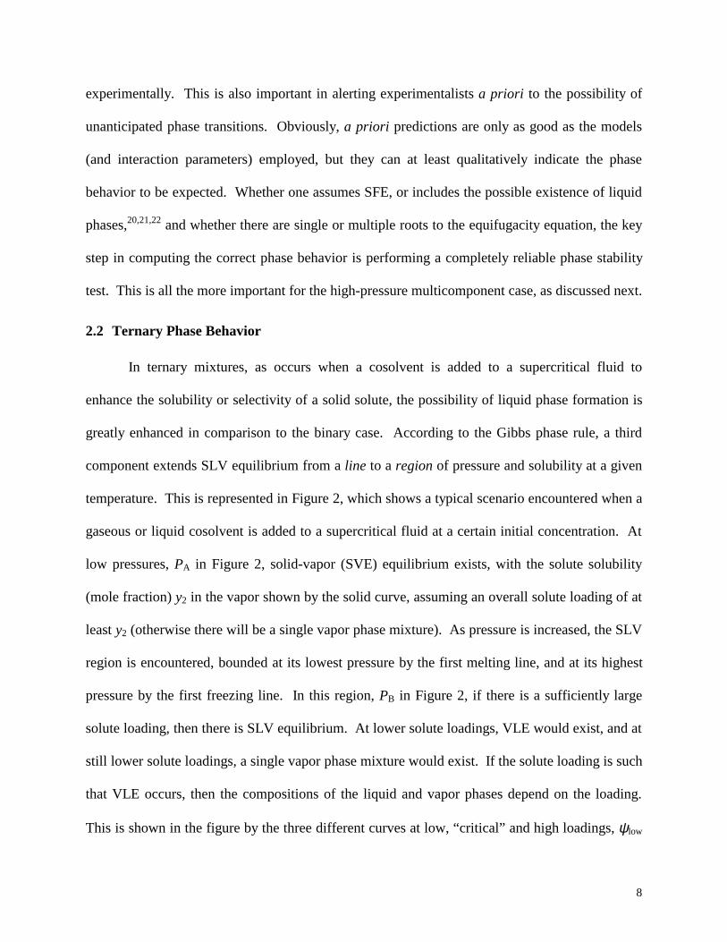
Figure 3 illustrates the low-pressure condition, PA from Figure 2. Each of the sides of the

triangle represents the conditions if the third component were absent: SLE for naphthalene and

propane (assuming that PA is greater than the vapor pressure of propane), SVE for naphthalene

and CO2, and a single phase for CO2 and propane (which assumes that the pressure is above the

mixture critical point of this binary). Since the constant solvent/cosolvent ratio line only passes

through the SV equilibrium and single-phase vapor sections of the diagram, these are the only

10

types of phase behavior that can exist at this pressure. There will be a single vapor phase if the

solute loading is very low, and SVE if the solute loading is high enough to put the overall

mixture composition point into the SV region. If the cosolvent to solvent ratio were to be

increased, thus shifting the constant solvent/cosolvent ratio line to the right, then one might

observe other kinds of phase behavior, including SLV, VLE, SLE, single-phase liquid or single-

phase vapor, depending on the solute loading.

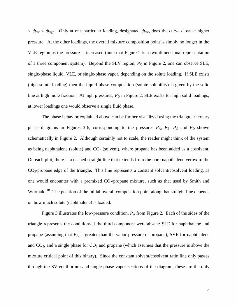
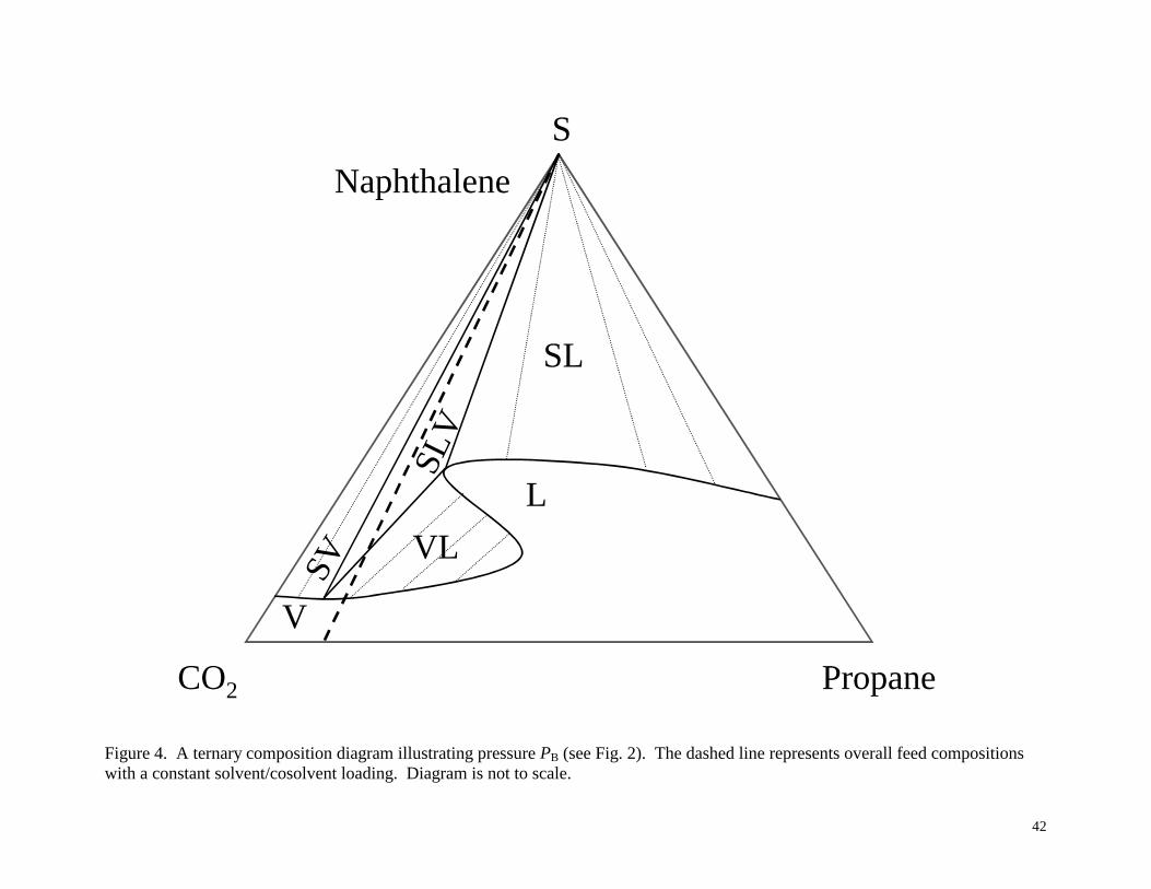
Figure 4 illustrates pressure PB, which cuts through the SLV region in Figure 2. SLV

equilibrium is found within a triangular region where the compositions of the phases are found at

the vertices of the SLV triangle, which includes pure solid naphthalene. At high solute loadings

(anywhere within the SLV triangle) SLV equilibrium occurs, while at smaller solute loadings

along the constant solvent/cosolvent ratio line, VLE is encountered. Note that, even though there

is an overall constant solvent/cosolvent ratio, in SLV and VLE the solvent/cosolvent ratio in

each phase is different. From this diagram it is also easy to see why the vapor and liquid

compositions in VLE depends on the solute loading, as this determines the tie line representing

the equilibrium.

A common feature of Figures 3-6 is the “S” shaped curve that extends from the

naphthalene/propane side of the triangle to the naphthalene/CO2 side. Notice its movement

towards the naphthalene/CO2 side with an increase in pressure, as seen from Figure 3 to Figure 6.

As the “S” shaped curve (and its associated phase equilibrium features) moves towards the

naphthalene/CO2 side the constant solvent/cosolvent ratio line passes through increasingly more

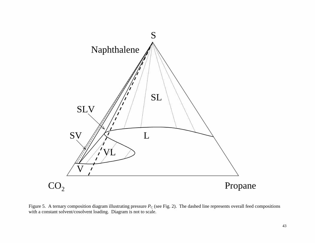
complex phase behavior, as shown by the triangular diagram for pressure PC in Figure 5. For the

solvent/cosolvent ratio shown by the straight dashed line, one can observe SLE, single-phase

liquid, VLE, or single-phase vapor, depending on the solute loading. Note that the phase

11

behavior would be SVE if the propane cosolvent were not present. However, with the propane

present there is the possibility of liquid phase formation. From Figure 5 it is also easy to see why

some of the VLE curves in Figure 2 terminate. For example, one can identify loadings on the

constant solvent/cosolvent ratio line that were in the VLE envelope in Figure 4 but that are in the

single phase liquid region in Figure 5. Thus, the VLE envelope of these loadings would

“terminate” at a pressure between PB and PC, as shown by ψhigh in Figure 2.

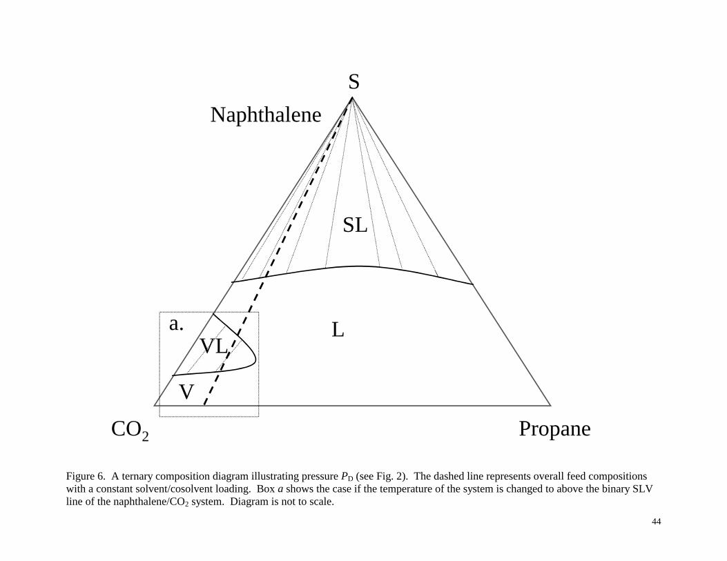
As shown in Figure 6 (neglecting box a for now), with a further increase in pressure to

PD the constant solvent/cosolvent ratio line no longer intersects the VLE envelope, and there

remains only one dense liquid-like state for SFE at high solute loading, and a single fluid phase

at lower solute loading. However, if the temperature of the system is changed to above the

binary SLV line of the naphthalene/CO2 system, then a VLE dome will appear emanating from

the naphthalene/CO2 side of the triangle, as shown in box a in Figure 6.

Thus, ternary and higher multicomponent systems exhibit many possibilities for complex

phase behavior, including the formation of liquid phases. As a result, there is a strong need for

reliable techniques to compute the high-pressure phase behavior of such systems. We will

demonstrate here a technique based on interval analysis that can provide a guarantee that the

phase equilibrium computations give correct results.

3. PROBLEM FORMULATION

To solve the phase equilibrium problem, it is first assumed that there is solid-fluid

equilibrium and then the corresponding equifugacity conditions are solved for all roots. The

roots are then tested using tangent plane analysis to determine if any represents a stable phase

equilibrium state. If no stable roots are found, then this indicates that at the specified

temperature, pressure, and overall composition, there is no solid-fluid equilibrium. In this case,

12

the problem is treated as a general multiple-fluid-phase flash with possible solid phase. In this

section, we summarize the formulation of each of these parts of the overall computation.

3.1 Equifugacity Conditions

The formulation used for the equifugacity conditions is developed in detail by Xu et al.7,

and is summarized briefly here. The species in the multicomponent system are designated as

solvent (component 1), solute (component 2), and cosolvent (components 3, 4, …, C). Assuming

a pure solid solute phase in equilibrium with a single fluid phase containing all components, then

the equifugacity conditions are:

( ) ( )y,,,ˆ, F2

S2 vPTfPTf =

(1)

11

=∑=

C

iiy

(2)

( ) ( )( ) ( ))()()(

,

)(,,

mmm

m

mP yyy

yy

ybvbbvv

Ta

bv

RTvTP

−++−

−=ℑ=

(3)

ii yy α=1 , i = 3, ..., C.

(4)

Here Eq. (1) is the equifugacity equation for the solute, with S2f indicating the fugacity of the

solute in the pure solid phase, F2f̂ the fugacity of the solute in the fluid-phase solution, v the

molar volume of the fluid phase, and y = (y1, y2, ..., yC)T the vector of fluid-phase mole fractions.

Equation (3) is the equation of state (EOS) for the fluid phase, and indicates the use of the Peng-

Robinson (PR) EOS. Here am and bm are the mixture attractive energy and co-volume

parameters of the PR EOS, and these are determined using standard (van der Waals) mixing

rules. Equation (4) specifies the molar solvent to cosolvent ratios iα for each cosolvent. The

13

ratios iα are specified, as are the system temperature T and pressure P. Equations (1-4) thus

represent a system of C+1 equations that can be solved for the C+1 variables y and v. Once y

has been determined, the molar phase fraction β S of the solid phase can be determined from the

solute material balance

,)1( 2S

2S ψββ =−+ y (5)

where ψ2 is the specified overall mole fraction of solute (overall solute loading). In solving Eqs.

(1-4) it is important to realize that there may be multiple solutions. To ensure that the phase

equilibrium problem is correctly solved, it is necessary to find all the equifugacity roots. A

solution method, based on interval mathematics, that can deal rigorously with the issue of

multiple solutions is discussed below.

There are alternative methods for determining the pure solid phase fugacity S2f , based on

the type of physical property data that is available. In the examples below, unless otherwise

noted, an expression based on sublimation pressure data is used:

( ) ( ) ( )( ).exp,

sub2

S2sub

2S

2

−=

RT

TPPvTPPTf (6)

Here sub2P is the solute sublimation pressure and S

2v is the molar volume of the pure solid

(assumed constant). An alternative expression18, used in some cases for consistency in making

comparisons to the literature, is

( ) ∫ −−

−∆=

P

TPdP

RT

vPTv

TTR

h

vPTf

PTf

)(sub2

SL

m

fus2

LL2

S2 ),(11

),,(

,ln (7)

Here L2f and Lv refer to a hypothetical subcooled pure liquid solute and are based on the fluid-

phase EOS, and fus2h∆ and Tm are the experimental molar heat of fusion and normal melting

temperature.

14

3.2 Stability Analysis

Solutions to the equifugacity conditions may represent stable, metastable or unstable

states. Since carefully measured equilibrium data most likely represent thermodynamically

stable data, it is desirable to deal exclusively with stable computational results. For this purpose,

tangent plane analysis23 is widely used. A fluid phase of composition (mole fraction) y0 is not

stable (i.e., unstable or metastable) if the Gibbs energy vs. composition surface ever falls below a

(hyper)plane tangent to the surface at y0. The Gibbs energy surface here consists of two parts,

one corresponding to the fluid phase (or phases), and another corresponding to the solid phase.

For the fluid case, we will express the Gibbs energy surface using gm(y,v), the (molar) Gibbs

energy of mixing (i.e., the Gibbs energy relative to pure component fluids at the system

temperature and pressure). Here v and gm are determined using the fluid-phase EOS; if there are

multiple volume roots, then the one yielding the smallest value of gm must be used. For the solid

case, since a solid phase is assumed to consist of pure solute, its part of the Gibbs energy vs.

composition surface consists of only a single point, which lies on the pure solute axis. Relative

to pure fluid solute at the system temperature and pressure (to be consistent with the reference

state used for the fluid-phase surface gm), this point has a (molar) Gibbs energy value

=

F2

S2S

2 lnf

fRTg (8)

Here S2f is determined from either Eq. (6) or (7), and F

2f is computed using the EOS with y2 =

1. This representation of the Gibbs energy surface is discussed in much more detail by Xu et al.7

and Marcilla et al.24

The distance between the Gibbs energy surface and the tangent plane is referred to as the

tangent plane distance. A plane tangent to the Gibbs energy surface at the fluid phase

15

composition y0 is given by

( ) ( ) ( )∑=

−

∂∂

+=C

iii

im yy

y

gvgg

10,

m00

tanm

0

,y

yy . (9)

Relative to the fluid phase Gibbs energy surface, the tangent plane distance is then

( ) ( )yyy tanm

F ,),( gvgvD m −= (10)

and relative to the solid phase it is

( )12tanm

S2

S =−= yggD (11)

If DF is negative for any value of y, or if DS is negative, then this indicates that the Gibbs energy

surface is below the tangent plane and thus the phase of composition y0 being tested is not stable.

If y0 is a solution to the equifugacity conditions for solid-fluid equilibrium, then the

tangent plane will pass through S2g (see Xu et al.7 and Marcilla et al.24 for discussion) and thus

DS is zero. Otherwise, the sign of DS can be checked by a straightforward point evaluation. To

determine if DF ever becomes negative is a much more challenging problem. This is typically

done by seeking the minimum of DF with respect to y by finding its stationary points in the space

constrained by the yi summing to one. However, it is common for there to be multiple local

minima in DF, and thus it is critical that the global minimum be found. If the global minimum of

DF is negative, then the phase being tested is not stable; otherwise it is stable. While only the

global minimum needs to be found for purposes of the stability analysis, it is in fact useful to

find the other stationary points as well, since as noted below, when the phase being tested is not

stable, the stationary points are useful in initializing subsequent phase split computations. A

solution method, again based on interval mathematics, that can deal rigorously

16

(deterministically) with the issue of the global minimization, as well as finding all the stationary

points, is discussed below.

3.3 Multiple-Fluid-Phase Flash with Possible Solid Phase

If it is determined that there are no solutions of the equifugacity conditions for solid-fluid

equilibrium that correspond to a stable equilibrium state, then there is no solid-fluid equilibrium

at the specified temperature, pressure, and overall composition. In this case, the problem is now

treated as a general multiple-fluid-phase flash with a possible solid phase. There are now many

flash algorithms for multi-fluid-phase equilibrium, of which the algorithm of Lucia et al.25 is

especially reliable (though not guaranteed). However, there are few flash algorithms for the case

of multiple fluid phases in equilibrium with a solid phase at high-pressures, using an EOS model

for the fluid phases; see Zhou et al.26 for example.

The method used here is a two-stage approach that alternates between phase split and

phase stability calculations. In the phase split problem, the number of fluid phases and whether

or not a solid phase is present is first postulated, generally based on information from a

preceding phase stability analysis, and then the corresponding Gibbs energy minimization

problem is solved for a potential equilibrium state. If there are NP fluid phases, labeled I, II, …,

NP, and a pure solid solute phase, labeled S, then the minimization problem is:

( ) ( ) ( ){ }S2

Sm

IIIIIIm

IIIIIm

I ,,,min gvgvgvg NPNPNPNP ββββ ++++ yyy ë (12)

subject to the mole fractions summing to one in each phase, the EOS in each phase, and the

overall material balance

1SIII =++++ ββββ NPë (13)

17

1-,1,2,i ,IIIIII Czyyyy iSi

SNPi

NPii ëë ==++++ ββββ , (14)

where β j is the molar phase fraction for phase j and zi indicates the overall mole fraction of

species i. Note that 1S2 =y and that 0S =iy , i ≠ 2, since the solid phase is pure solute. For the

solute, z2 equals ψ2, the specified fractional loading of solute in the system being studied. For

the solvent and cosolvents, the zi are readily determined from the specified solvent to cosolvent

ratios αi together with the summation of the zi to one. In solving this optimization problem, one

needs to find only a local minimum, since if the global optimum is not found, this will be

detected in the subsequent phase stability analysis, which in effect is a global optimality test.

Good initial guesses for the local optimization can generally be obtained by using stationary

points from the preceding stability analysis. For solving this optimization problem, we use the

successive quadratic programming (SQP) approach described and implemented by Chen and

Stadtherr.27 However, there are many other approaches that could be used to perform this local

optimization, and that may perform better than SQP in this context. Furthermore, there are

alternative problem formulations that could be used; for example, the use of mole numbers rather

than mole fractions as independent variables. It is not critical in the phase split computation

what approach is used, as long as it converges to a local minimum in the Gibbs energy.

Once a potential equilibrium state is found by locating a minimum in the optimization

problem, then it is tested using phase stability analysis, as described above. If this indicates that

the state is not stable, then either 1) the phase-split optimization problem is solved again with the

same number and type of phases, but with new initial guesses based on the newly found

stationary points, or 2) the phase-split optimization problem is reformulated by adding a new

phase. This type of two-stage strategy that alternates between phase split and phase stability

calculations is widely used for the case in which there are fluid phases only25,28,29, and can be

18

shown30 to converge in a finite number of steps to the equilibrium solution, provided that the

phase stability problem is solved to global optimality.

4. SOLUTION METHODOLOGY

To correctly solve the problems formulated above, it is necessary to have a procedure that

is capable of reliably locating all the solutions of a nonlinear equation system and to have a

deterministic procedure that is capable of locating the global optimum of a nonlinear function.

These capabilities can be provided through the use of interval analysis.

4.1 Interval Analysis

Good introductions to interval analysis, as well as to interval arithmetic and computing

with intervals, include those of Neumaier31, Hansen32 and Kearfott.33 Of particular interest here

is the interval-Newton/generalized bisection (IN/GB) technique. Given a nonlinear equation

system with a finite number of real roots in some specified initial interval, this technique

provides the capability to find (or, more precisely, to enclose within a very narrow interval) all

the roots of the system within the given initial interval. This can be applied directly to the

solution of the equifugacity conditions, as formulated above. To apply this technique to the

minimization problem of interest in phase stability analysis, IN/GB is used to solve a nonlinear

equation system for all the stationary points in the optimization problem. Alternatively, this can

be done in combination with a simple branch-and-bound scheme, so that all the stationary points

do not need to be found, only the one corresponding to the global minimum. However, as noted

above, knowledge of the stationary points may be useful for initializing the phase split

computations, so we typically use IN/GB to find all the stationary points. These procedures are

19

outlined in more detail by Xu et al.7, and further details are given by Hua et al.34,35 and

Schnepper and Stadtherr.36

Properly implemented, the IN/GB technique provides the power to find, with

mathematical and computational certainty, enclosures of all solutions of a system of nonlinear

equations, or to determine with certainty that there are none, provided that initial upper and

lower bounds are available for all variables.31,33 This is made possible through the use of the

powerful existence and uniqueness test provided by the interval-Newton method. The technique

can also be used to enclose with certainty the global minimum of a nonlinear objective

function32, again assuming an initial interval is provided for all variables. Note that unlike

standard local equation-solving and optimization routines, which require a point initialization,

the IN/GB approach requires only an initial interval. Since this initial interval can be made

sufficiently large to include all physically feasible possibilities, this makes the methodology

essentially initialization independent. The interval methodology has been successfully applied to

solve a wide variety of thermodynamic phase behavior problems.7,37,38 The overall strategy for

solving the phase behavior problem of interest here is outlined below.

4.2 Problem-Solving Strategy

It is first assumed that there is solid-fluid equilibrium, so the equifugacity conditions,

Eqs. (1-4), are solved using the interval methodology. From Eq. (5), it is clear that 0 ≤ y2 ≤ ψ2,

thus the initial interval for y2 is [0, ψ2]. Initial intervals for the remaining fluid-phase mole

fractions yi can then be determined from Eqs. (2) and (4), using interval arithmetic and the initial

interval for y2. In the initial interval for v, the lower bound is taken to be the smallest of the pure

component co-volume parameters, that is, mini bi, and the upper bound is taken to be 2RT/P

20

(compressibility factor of 2). Application of the IN/GB approach will now determine all roots, if

any, within these initial intervals.

One possibility is that there could be one or more equifugacity roots. In this case, each

root is tested for phase stability as described above, using the interval methodology to assure

correct results. For solving the phase stability problem, each mole fraction yi has the initial

interval [0, 1], and the initial volume interval is the same as used in solving the equifugacity

condition. If there is a root that tests stable, then a solid-fluid equilibrium state has been found.

It is also possible that more than one equifugacity root will test as stable; this indicates an

equilibrium state with a solid phase and multiple fluid phases (corresponding to the multiple

stable equifugacity roots). If none of the roots test as stable then there is no solid-fluid

equilibrium state. In this case, we postulate two fluid phases plus a solid phase, and initiate the

two-stage procedure described in section 3.3 that alternates between phase split and phase

stability calculations until the correct number and type of phases and phase compositions are

found. The result will be multiple-fluid-phase equilibrium that may or may not include a solid

phase. The procedure used is a modification of the INTFLASH routine described by Hua39 and

also applied by Stradi et al.40 and Xu et al.7 The original INTFLASH performs multiple-fluid-

phase flash calculations; the modification accounts for the possibility of a pure solid phase also

present.

Alternatively, another possibility is that there could be no equifugacity roots. This

indicates that the solute loading ψ2 was sufficiently small that all the solid dissolved. Thus, a

single fluid phase with y2 = ψ2 is next postulated, and this is tested for phase stability as

described above. If the test indicates stability, then the equilibrium state is a single fluid phase

with y2 = ψ2; otherwise two fluid phases are next postulated, and we again initiate the two-stage

21

procedure described in section 3.3 that alternates between phase split and phase stability

calculations until the correct number of phases and phase compositions are found.

5. RESULTS AND DISCUSSION

5.1 _ Example 1: Naphthalene and CO2 with Gaseous Cosolvents Ethane and Propane

The solubility of naphthalene in the solvent/cosolvent mixtures CO2/C2H6 and CO2/C3H8

has been investigated by Smith and Wormald.18 Both systems were measured at temperatures

from 35 °C to 60 °C, and at pressures from 60 to 250 bar. They also determined the SLV

equilibrium (first melting line) for these systems, and modeled the data using the Peng-Robinson

EOS with van der Waals mixing rules. Their model computations were based on the

equifugacity condition, using Eq. (7) for the solid fugacity, but without stability analysis. For

their model, they took values of the binary interaction parameters k12 and k13 from the literature,

and fit values of k23 to their experimental solubility versus pressure data. Exactly the same

model is used for the computations done in this example. The binary interaction parameter

values18 used are k12 = 0.090, k13 = 0.131 (3 = ethane), k13 = 0.125 (3 = propane), k23 = 0.040 (3 =

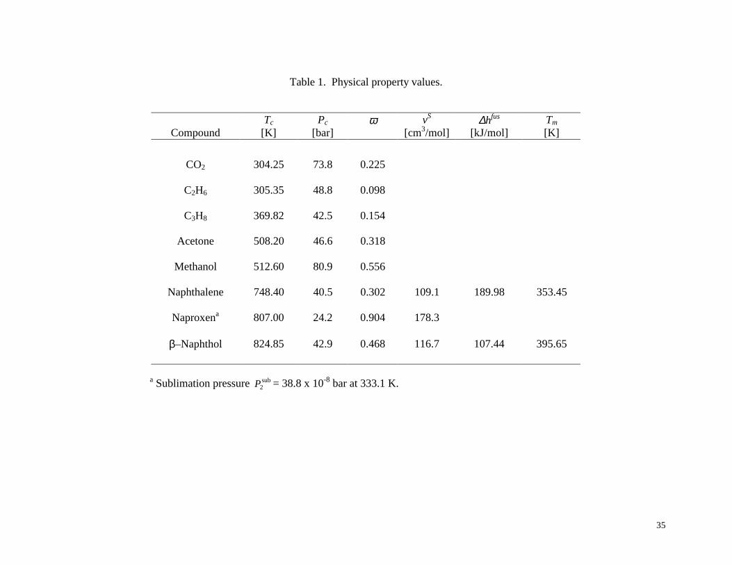
ethane) and k23 = 0.041 (3 = propane). Other physical property data used in the model are given

in Table 1.

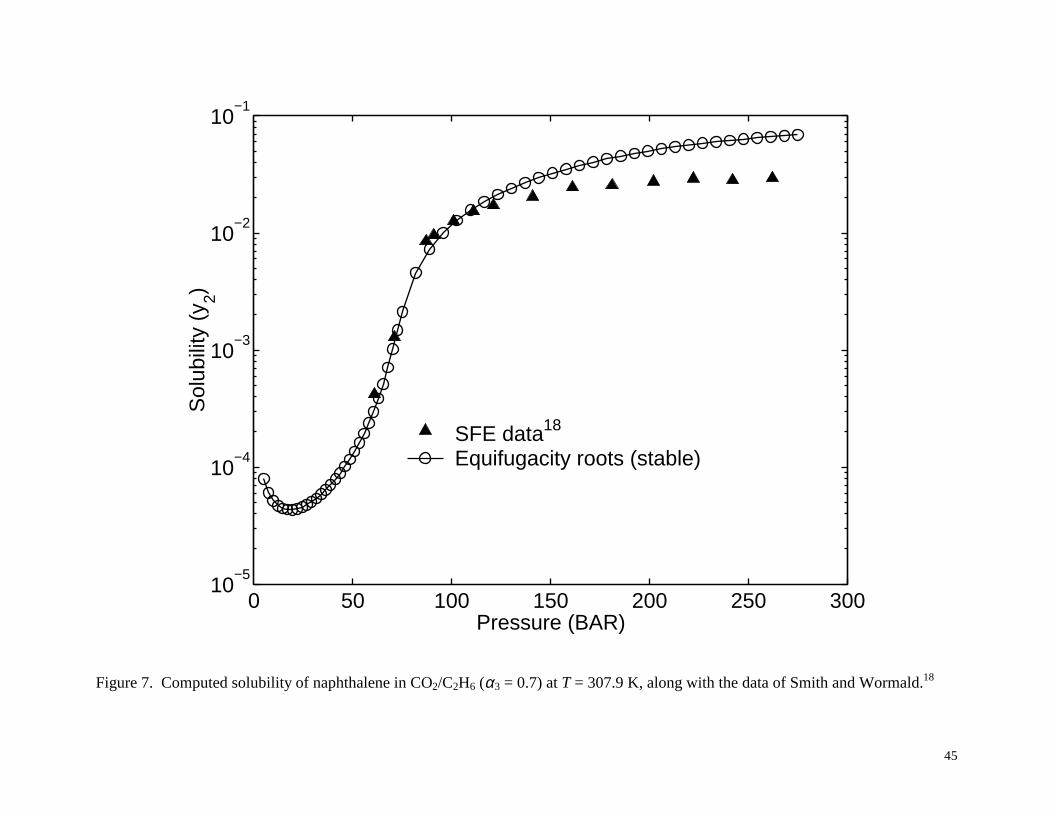
Using the strategy described in Section 4.2, the solubility y2 of naphthalene in CO2/C2H6

(α3 = 0.7) and CO2/C3H8 (α3 = 5.6) was computed at several temperatures over a pressure range

that includes the range studied by Smith and Wormald. Figure 7 shows the computed results for

CO2/C2H6 at T = 307.9 K, along with the data of Smith and Wormald18. As shown, at each

pressure there is a single solubility root to the equifugacity condition, which was confirmed to be

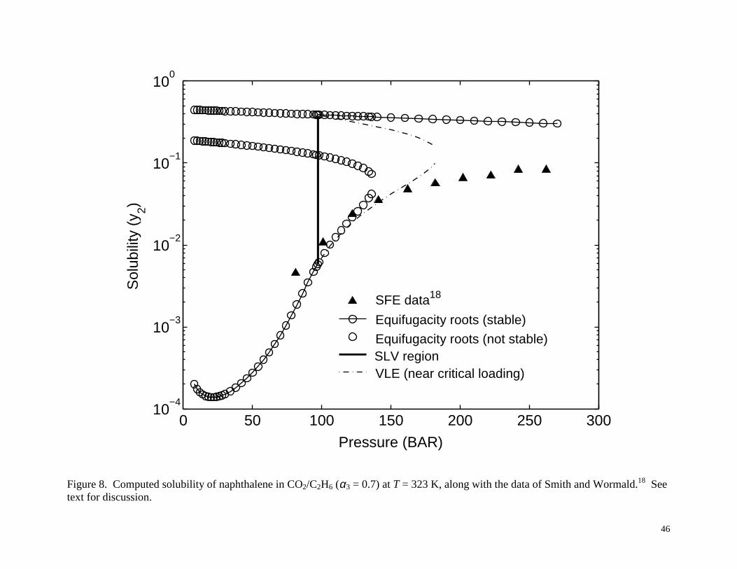
stable using the interval method. Figure 8 shows the results for T = 323 K. Here there is a large

22

range of pressure for which there are three equifugacity roots. The roots representing stable

equilibrium are denoted by the solid curve. At lower pressures (below about 100 bar), the

smallest solubility root is stable, implying solid-vapor equilibrium. Then, according to Smith

and Wormald’s model18, around 100 bar, a very small region (which appears in Figure 8 as a

heavy vertical line) of SLV equilibrium appears, bounded by the first melting and last freezing

pressures. In this pressure region, Smith and Wormald’s model18 indicates that large solute

loadings result in SLV equilibrium, i.e., liquid phase formation, and at lower loadings VLE

exists, with phase compositions determined by the solute loading (see Section 2.2). At pressures

above the SLV region, the highest solubility root is stable, implying solid-liquid equilibrium

provided that the solute loading is sufficient. At lower solute loadings there can be VLE with the

phase compositions varying according to the loading. In Figure 8, the VLE region is shown as a

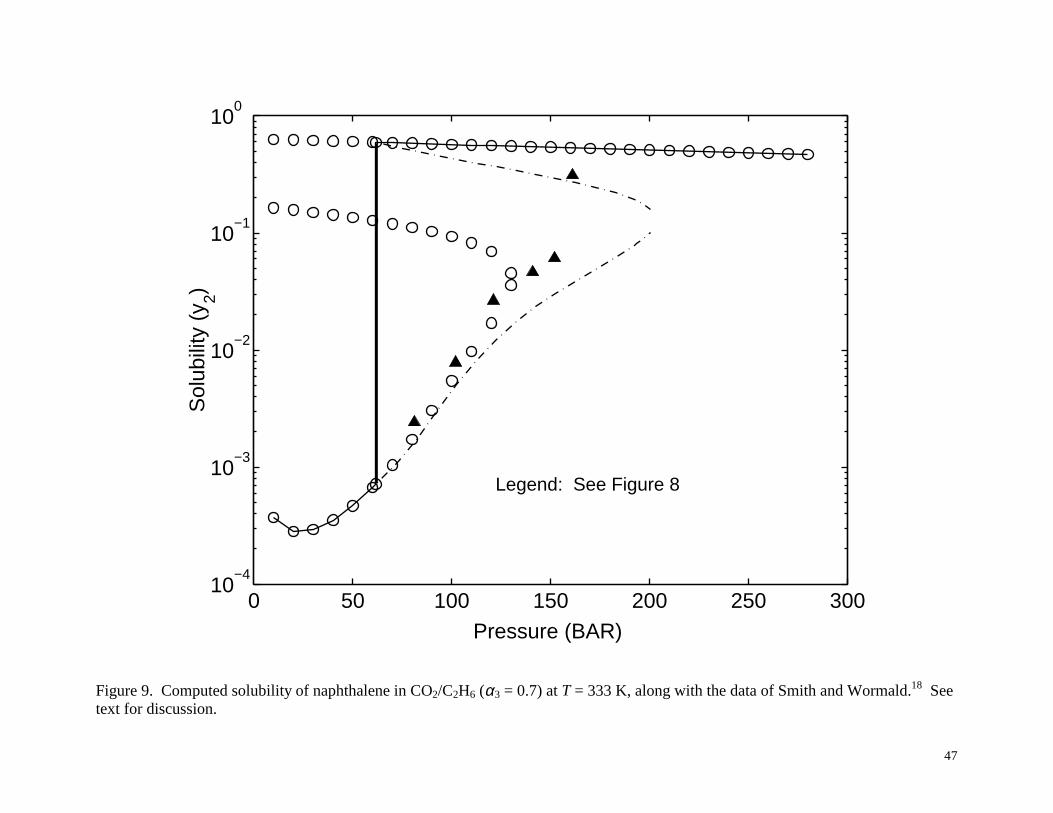
dashed-dotted line for the case of a near critical loading. Figure 9 shows the results for T =

333 K for the Smith and Wormald model18, which are qualitatively similar to the 323 K case.

Here the SLV region is again very narrow, from about 61.75 to 62.25 bar. Clearly, for the

situations depicted in Figures 8 and 9, reliable stability analysis is critical in determining the

nature of the phase behavior predicted by the model.

For the 323 K and 333 K cases (Figures 8 and 9) there is a discrepancy between the SFE

data of Smith and Wormald18 and the stable SFE predicted by their model. In other words, there

is an inconsistency between Smith and Wormald’s reported experimental data and their model.18

This means one of two things. One possibility is that the model is simply inadequate. This could

be due to a fundamental inability of the simple Peng-Robinson equation to model this system, or,

perhaps, it could be due to a significant temperature dependence of one or more of the binary

interaction parameters that is not taken into account. Another possibility is that the experimental

23

SFE results reported are not really SFE. We have some additional insight into this system

because Smith and Wormald18 also measured the SLV equilibrium (first melting curves).

Interestingly, the experimental SLV lines that Smith and Wormald18 report confirm that portions

of their SFE data actually reside inside the VLE region, similar to the results obtained by their

model. However, since the measurements were taken in a flow apparatus, they may not be

meaningful VLE data. For ternary systems, VLE is dependent on the overall loading of the

components, with different loadings producing different compositions in each phase. Thus for

VLE data to be meaningful, the overall composition it corresponds to must be known. However,

in a flow system the loadings are constantly changing, and so in principle the overall

composition is not known. In practice it may be that the loadings will undergo only insignificant

changes, though, if so, this should be determined a priori.

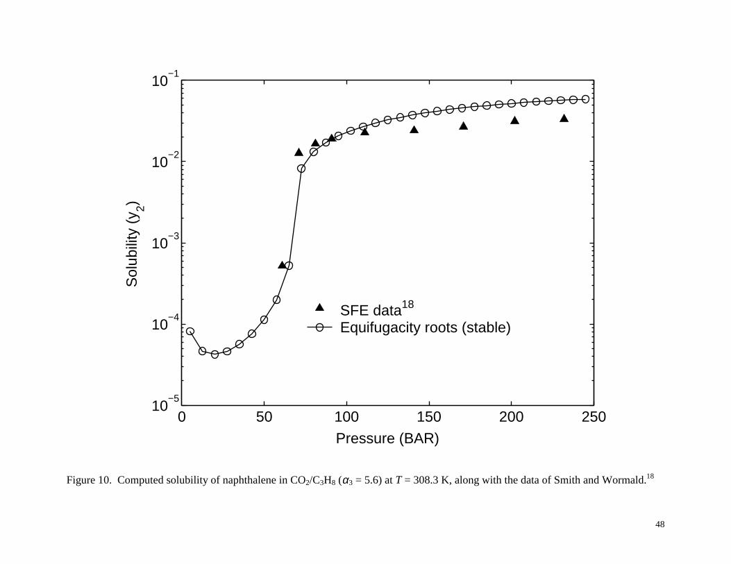
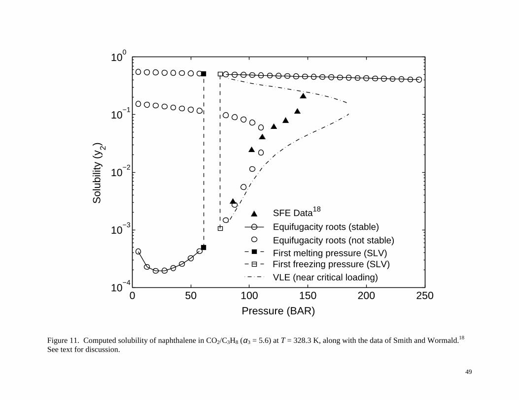
Figures 10 and 11 show the results for the case of propane as cosolvent with α3 = 5.6. At

T = 308.3 K, as shown in Figure 10, there is a single stable solubility root to the equifugacity

condition, similar to the situation in Figure 7 for the ethane cosolvent. At T = 328.3 K, as shown

in Figure 11, there are multiple equifugacity roots, and the situation is similar to that shown in

Figures 8 and 9 for the ethane cosolvent. In this case, however, the SLV region is much wider,

ranging from about 62 to 78 bar, due to the fact that CO2 and propane are chemically less similar

than CO2 and ethane. Again, there is an inconsistency between the data and the model used by

Smith and Wormald.18 Either the model is totally inadequate or the experimental phase

equilibrium has been misidentified. If the latter is the case, then it would mean that the

experimental data reported as SFE by Smith and Wormald18 might actually be VLE which is

predicted by their model, assuming an appropriate solute loading.

24

5.2 Example 2: Naproxen and CO2 with a Liquid Cosolvent

The solubility of naproxen in supercritical CO2 with various cosolvents was measured

and modeled by Ting et al.41 They studied the cosolvents acetone, ethyl acetate, methanol,

ethanol, 1-propanol and 2-propanol. These cosolvents are liquids at ambient conditions and are

different than the nonpolar gases that served as cosolvents in the previous example. The

presence of a highly asymmetric cosolvent (whose polarity and critical properties are very

different than those of CO2) provides for even richer phase behavior than that shown

schematically in Figures 2-6. Due to the possible association between the cosolvent and the

solute, naproxen, the experimental solubility enhancement was considerable compared with the

cosolvent-free case. They qualitatively represent the solubility enhancement by using the

concept of the cosolvent effect, which is defined as the ratio of the solubility obtained with the

cosolvent to that obtained without cosolvent at the same temperature and pressure. It was

demonstrated that the cosolvent effect (increase in solubility with the cosolvent) increases in the

order ethyl acetate, acetone, methanol, ethanol, 2-propanol and 1-propanol.

Ting et al.41 believed that no liquid phase formed throughout their experiments,

substantiated by no evident melting in their samples after depressurization. Therefore, they

assumed a solid-fluid equilibrium model and then regressed interaction parameters for the Peng-

Robinson EOS with van der Waals mixing rules. As discussed above, if two-phase solid-fluid is

the true equilibrium state, then the fluid phase itself must be thermodynamically stable.

However, using the procedure for stability analysis described above demonstrates that this is not

true for all temperatures and pressures investigated. In other words, there is an inconsistency or

mismatch between the data and the model presented by Ting et al.41 As described in Example 1,

this means one of two things. One possibility is that the model presented by Ting et al.41 is

25

inadequate, i.e., it is not able to describe the real phase behavior with the parameters they used.

A second possibility is that the experimental data, which was presented as SFE, was actually not

SFE.

As a specific example, consider the case of acetone as cosolvent (α3 = 96.5/3.5) at T =

333.1 K. Using the binary interaction parameter values k12 = 0.229, k13 = 0 and k23 = -0.196

regressed by Ting et al.41, the physical property values estimated by Ting et al.41 (see Table 1),

and the computational procedure given above, the true equilibrium state predicted by the Peng-

Robinson EOS with van der Waals mixing rules has multiple fluid phases, except at the two

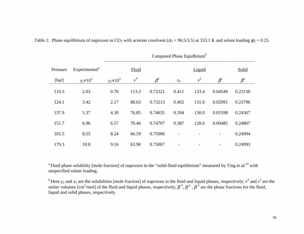
highest pressures considered (165.5 and 179.3 bar). Table 2 shows results for the case in which

the initial solute loading is ψ2 = 0.25, which is sufficiently high to give SLV equilibrium. If the

solute loading is lower, the results are VLE (except at 165.5 and 179.3 bar), with the phase

compositions dependant on the specific solute loading. The experimental data, identified by

Ting et al.41 as solid-fluid equilibrium, are also listed for comparison. The fact that the

experimental solubilities are fairly close to the computed solubilities for the SLV case, suggests

that experimentally there might have been a liquid phase present. If experimental SLV data were

available, better interaction parameters values could then be regressed from this data. If in fact

there was small amount of liquid phase present in the experimental measurements, then this

could have a significant impact on the physical interpretation of the cosolvent effect, since the

concentration of solute in this phase is quite high. While we have focused in this example on the

acetone cosolvent case, the same issue (model predicts that the fluid phase is not stable) occurs

with the other cosolvents studied as well.

One can learn from this example that, without reliable computation of phase stability,

experimental data may end up being fit to an unstable solution of a thermodynamic model, thus

26

leading to misinterpretation of both experimental and modeling results. The investigators of this

system inferred from their observations that there was no liquid phase present, though liquid

phase formation might be difficult to observe due to the small liquid phase fraction and

insufficient equilibration time for melting. With the current parameters, this model predicts SLV

equilibrium, not SFE as the modelers intended. This suggests the need for further studies into

this cosolvent system in a static high-pressure view cell to ascertain its true phase behavior.

Once determined, interaction parameters that predict the true stable equilibrium could be

regressed, which would lend greater confidence to process design and simulation.

5.3 Example 3: ββββ–Naphthol and CO2 with Methanol Cosolvent

The system of β–naphthol/CO2 with a methanol cosolvent was investigated by Dobbs et

al.,42 Dobbs and Johnston,43 and Lemert and Johnston.44 The solubility of β-naphthol in CO2

mixtures with as much as 9.0 mole % methanol were measured by Dobbs and Johnston43, and

SLV equilibrium was measured and modeled by Lemert and Johnston44 up to 4.0 mole %

methanol. Lemert and Johnston44 calculated the SLV equilibrium (“first melting” line) by

specifying the pressure and determining the lowest temperature yielding SLV equilibrium. In

other words, for a given pressure and solvent/cosolvent ratio, the system is a solid phase in

equilibrium with a single vapor or fluid phase until the temperature is raised high enough to

cause melting; this is the temperature corresponding to the “first melting” line found by Lemert

and Johnston.44 Especially when cosolvents are present, this SLV line can be significantly below

the normal melting point of the solid. The SLV line was computed from the equifugacity

relationship using the Peng-Robinson equation of state for the vapor phase, Regular Solution

Theory for the liquid phase fugacity, Eq. (7) for the solid phase, and the physical property data

given in Table 1. The experimental SLV equilibrium and the model agreed well.

27

The computational procedure that we have described above can also be used to detect the

SLV equilibrium (“first melting” line) in a typical extraction situation, such as this, that involves

cosolvents. Our model is similar to that of Lemert and Johnston44 except that we use the

equation of state for both the liquid and vapor phases. For a given pressure we found the lowest

temperature that yielded three roots to the equifugacity equation with two roots being

thermodynamically stable, thus indicating two fluid phases in equilibrium with the solid phase.

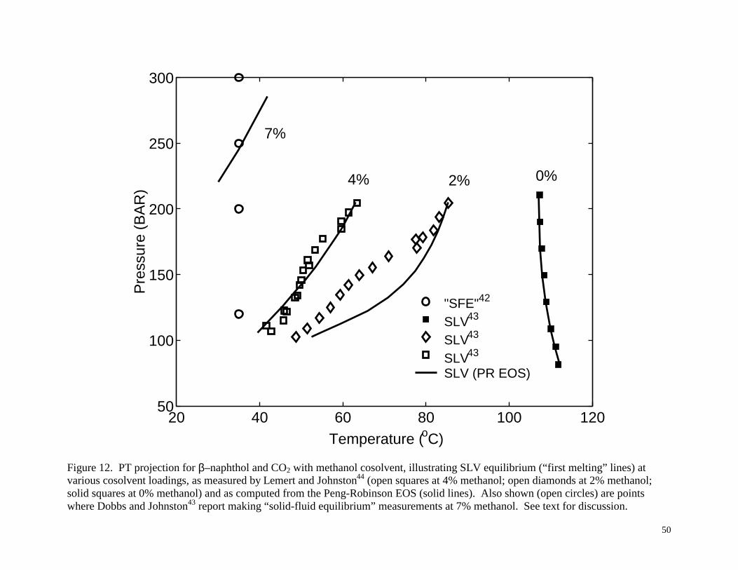
Figure 12 illustrates the experimental SLV data from Lemert and Johnston44 with increasing

concentrations of methanol from right to left. Also shown are the corresponding first-melting

SLV curves from our Peng-Robinson model using parameters of k12=0.0230, k13=-0.0475, and

k23=0.1675. The model can be seen to be in good agreement with the experimental

measurements, and it matches closely the model results of Lemert and Johnston44. Note that the

SLV lines with cosolvent slope upward (positive slope) so that at temperatures greater than and

pressures less than the first melting SLV lines, one could observe a stable liquid phase.

We also performed the calculations for higher methanol concentrations, such as the 7.0

mole % methanol first-melting SLV curve shown in Figure 12. Based on these calculations,

using a 7 mole % methanol/CO2 solution at 35°C to extract β-naphthol should result in liquid

phase formation at any pressure less than about 250 bar. The type of phase behavior, i.e., SLVE

or VLE, would depend on the loading of solute. Yet, measurements identified as solid-fluid

equilibrium by Dobbs and Johnston,43 were as low as 120 bar for the 7.0 mole % methanol case.

Once again, there are two possibilities. One possibility is that the model we have used gives a

good representation of the SLV curves at 0, 2 and 4 mole % methanol but is not able to predict

the 7 mole % methanol curve correctly; i.e., the model is wrong. The second possibility is that

the data of Dobbs and Johnston43 for 7.0 mole % methanol at 120 and 200 bar are not stable

28

solid-fluid equilibria. Rather, they may represent VLE data, which is not particularly meaningful

without knowing the solute loading, as was discussed above in Example 1. Whichever is the

case, one would certainly want to re-examine the phase behavior of the β-naphthol/CO2/7 mole

% methanol system at the lower pressures with a view cell to confirm which phases are actually

present before designing an actual separation process for this system.

5.4 Computational Performance

As might be expected, the guarantee of complete reliability in computing the equilibrium

state comes at some computational expense. However, for these three-component problems, the

cost is actually quite small. The computation times required vary somewhat from problem to

problem due to differences in the number of equilibrium phases and the number of stationary

points in the phase stability analysis. The case of the CO2-naproxen-acetone system at 333.1 K

is typical. Here for the pressures yielding SLV equilibrium, the CPU times are around 30

seconds, and for pressures yielding SFE around 10 seconds (all CPU times based on using a Dell

WorkStation 530MT at 2 GHz). These times are certainly much higher than what would be

required by standard local methods for computing phase equilibrium. However, such standard

methods offer no guarantee that the equilibrium state has actually been found. Thus, there is a

trade-off between computation time and reliability, and the modeler must decide how important

it is to know for certain that the correct answer has been obtained.

In the approach used here, essentially all the CPU time is spent in the phase stability

analysis stage of the problem, for which, as discussed above, the interval methodology of Hua et

al.35 is used. Another approach for reliable determination of phase stability from cubic EOS

models is that of Harding and Floudas45, who use a global optimization method based on branch-

and-bound using convex underestimating functions. However, this approach will not find all of

29

the stationary points of the tangent plane distance (useful to initialize the phase split

computations) and so is not directly comparable to the approach of Hua et al.35

6. CONCLUSIONS

We have presented a completely reliable solution strategy for computing high-pressure,

solid-multiphase equilibria, using cubic equations of state. The key to this technique is the use of

interval analysis to implement the thermodynamic stability test. This is an extension of our

previous work on the reliable computation of solid-fluid equilibria7 to include the presence of

cosolvents. Gaseous or liquid cosolvents are frequently used in supercritical fluid extraction

processes, and are integral in processes such as the gas anti-solvent process (GAS) to precipitate

uniform solid particles. Identifying the correct stable high-pressure phase equilibrium predicted

by a particular model can be very problematic for commonly used local solvers. This situation is

only further exacerbated when cosolvents are present. The presence of even chemical similar

cosolvents can induce complex phase behavior that may not be intuitive to either the

experimentalist or the modeler. Using several examples from the literature, we have

demonstrated how our new solution technique, based on interval analysis, can be used to identify

experimental data that may have been misinterpreted and to identify models that do not predict

what the modeler intended.

7. Acknowledgements

Financial support from the Department of Energy, under Grant DE-FG02-98ER14924,

the Petroleum Research Fund, administered by the ACS, under Grant 35979-AC9, the State of

Indiana 21st Century Research and Technology Fund, a Bayer Predoctoral Fellowship (A.M.S.),

and the University of Notre Dame Provost Fellowship (G.X.) is gratefully acknowledged.

30

References (1) McHugh, M. A.; Krukonis, V. J. Supercritical Fluid Extraction: Principles and Practice; 2nd

ed.; Butterworth-Heinemann: Oxford, U.K., 1994.

(2) Matson, D. W.; Fulton, J. L.; Petersen, R. X.; Smith, R. D. Rapid Expansion of Supercritical

Fluid Solutions: Solute Formation of Powders, Thin Films and Fibers. Ind. Eng. Chem. Res.

1987, 26, 2298-2306.

(3) Mohamed, R. S.; Debenedetti, R. G.; Prud’homme. R. K. Effects of Process Conditions on

Crystals Obtained from Supercritical Mixtures. AIChE J. 1987, 35, 325-328.

(4) Dixon, D.; Johnston, K. P. Molecular Thermodynamics of Solubilities in Gas-Antisolvent

Crystallization. AIChE J. 1991, 37, 1441-1449.

(5) Gallagher, P. M.; Coffey, M. P., Krukonis, V. J.; Klasutis, N. New Process to Recrystallize

Compounds Insoluble in Supercritical Fluids, in K.P. Johnston, J.M.L. Penninger (Eds.),

Supercritical Fluid Science and Technology, American Chemical Society, Washington, DC,

1989, p.334.

(6) Reverchon, E. Supercritical Antisolvent Precipitation of Micro- and Nano-Particles. J.

Supercrit. Fluids 1999, 15, 1-21.

(7) Xu, G.; Scurto, A. M.; Castier, M.; Brennecke, J. F.; Stadtherr, M. A. Reliable Computation

of High Pressure Solid-Fluid Equilibrium. Ind. Eng. Chem. Res. 2000, 39,1624-1636.

(8) McHugh, M. A.; Paulaitis, M. E. Solid Solubilities of Naphthalene and Biphenyl in

Supercritical Carbon Dioxide. J. Chem. Eng. Data 1980, 29, 326-328.

(9) McHugh, M. A.; Yogan, T. J. Three-Phase Solid-Liquid-Gas Equilibria for Three Carbon

Dioxide-Hydrocarbon Solid Systems, Two Ethane-Hydrocarbon Systems, and Two Ethylene-

31

Hydrocarbon Solid Systems. J. Chem. Eng. Data 1984, 29, 112-115.

(10) Brunner, G.; Peter, S. On the Solubility of Glycerides and Fatty Acids in Compressed

Gases in the Presence of an Entrainer. Sep. Sci. Tech. 1982, 17, 199-214.

(11) Joshi, D. K.; Prausnitz, J. M. Supercritical Fluid Extraction with Mixed Solvents. AIChE J.

1984, 30, 522-525.

(12) Ekart, M. P.; Bennett, K. L.; Ekart, S. M.; Gurdial, G. S.; Liotta, C. L.; Eckert, C. A.

Cosolvent Interactions in Supercritical Fluid Solutions. AIChE J. 1993, 39, 235-248.

(13) Dobbs, J. M.; Johnston, K. P. Selectivities in Pure and Mixed Supercritical Fluid Solvents.

Ind. Eng.Chem. Res. 1987, 26, 1476-1482.

(14) Jessop, P. G.; Ikariya, T.; Noyori, R. Homogeneous Catalysis in Supercritical Fluids.

Chem. Rev. 1999, 99, 475-493.

(15) De Swaans Arons, J.; Diepen, G. A. M. Thermodynamic Study of Melting Equilibria under

Pressure of a Supercritical Gas. Rec. Trav. Chim. Pays-Bas 1963, 82, 249-256.

(16) Luks, K. D. The Occurrence and Measurement of Multiphase Equilibria Behavior. Fluid

Phase Equil. 1986, 29, 209-224.

(17) van Welie, G. S. A.; Diepen, G. A. M. The solubility of Naphthalene in Supercritical

Ethane. J. Phys. Chem. 1963, 67,755-757.

(18) Smith, G. R.; Wormald, C. J. Solubilities of Naphthalene in (CO2 + C2H6) and (CO2 +

C3H8) up to 333 K and 17.7 MPa. Fluid Phase Equil. 1990, 57, 205-222.

(19) Koningsveld, R., Diepen, G. A. M. Supercritical Phase Equilibrium Involving Solids. Fluid

Phase Equil. 1983, 10, 159-172.

32

(20) Kikic, I.; Lora, M.; Bertucco, A. A. Thermodynamic Analysis of Three-Phase Equilibria in

Binary and Ternary Systems for Applications in Rapid Expansion of a Supercritical Solution

(RESS), Particles from Gas-Saturated Solutions (PGSS), and Supercritical Antisolvent (SAS).

Ind. Eng.Chem. Res. 1999, 36, 5507-5515.

(21) Lemert, R. M.; Johnston, K. P. Solid-Liquid-Gas Equilibria in Multicomponent

Supercritical Fluid Systems. Fluid Phase Equil. 1989, 45, 265-286.

(22) Da Rocha, S. R. P.; Oliveira, J. V.; d’Ávila, S. G. A. Three-Phase Ternary Model for CO2-

Solid-Liquid Equilibrium at Moderate Pressures. J. Supercrit. Fluids 1996, 8, 1-5.

(23) Baker, L. E.; Pierce, A. C.; Luks, K. D. Gibbs Energy Analysis of Phase Equilibria. Soc.

Pet. Eng. J. 1982, 22, 731-742.

(24) Marcilla, A.; Conesa, J. A.; Olaya, M. M. Comments on the Problematic Nature of the

Calculation of Solid-Liquid Equilibrium. Fluid Phase Equil. 1997, 135, 169-175.

(25) Lucia, A.; Padmanabhan, L.; Venkataraman, S. Multiphase Equilibrium Flash Calculations.

Comput. Chem. Eng. 2000, 24, 2557-2569.

(26) Zhou, X.; Thomas, F. B.; Moore, R. G. Modeling of Solid Precipitation from Reservoir

Fluid. J. Can. Pet. Tech. 1996, 35, 37-45.

(27) Chen, H. S.; Stadtherr, M. A. Enhancements of the Han-Powell Method for Successive

Quadratic Programming. Comput. Chem. Eng. 1984, 8, 229-234.

(28) Michelsen, M. L. The Isothermal Flash Problem. 1. Stability. Fluid Phase Equil. 1982, 9,

1-19.

(29) Michelsen, M. L. The Isothermal Flash Problem. 2. Phase-Split Calculation. Fluid Phase

33

Equil. 1982, 9, 21-40.

(30) McKinnon, K. I. M.; Millar, C. G.; Mongeau M. Global Optimization for the Chemical and

Phase Equilibrium Problem Using Interval Analysis. In State of the Art in Global Optimization:

Computational Methods and Applications; Floudas, C. A.; Pardalos, P.M., Eds.; Kluwer

Academic Publishers: Dordrecht, The Netherlands, 1996.

(31) Neumaier, A. Interval Methods for Systems of Equations; Cambridge University Press:

Cambridge, England, 1990.

(32) Hansen, E. Global Optimization Using Interval Analysis, Marcel Dekkar: New York, 1992.

(33) Kearfott, R. B. 1996, Rigorous Global Search: Continuous Problems; Kluwer Academic

Publishers: Dordrecht, The Netherlands.

(34) Hua, J. Z.; Brennecke, J. F.; Stadtherr, M. A. Reliable Computation of Phase Stability

Using Interval Analysis: Cubic Equation of State Models. Comput. Chem. Eng. 1998, 22, 1207-

1214.

(35) Hua, J. Z.; Brennecke, J. F.; Stadtherr, M. A. Enhanced Interval Analysis for Phase

Stability: Cubic Equation of State Models. Ind Eng. Chem. Res. 1998, 37, 1519-1527.

(36) Schnepper, C. A.; Stadtherr, M. A. Robust Process Simulation Using Interval Methods.

Comput. Chem. Eng., 1996 20, 187-199.

(37) Stradi, B. A.; Brennecke, J. F.; Kohn, J. P.; Stadtherr, M. A. Reliable Computation of

Mixture Critical Points. AIChE J. 2001, 47, 212-221.

(38) Maier, R. W.; Brennecke, J. F.; Stadtherr, M. A. Computing Homogeneous Azeotropes

Using Interval Analysis. Chem. Eng. Technol. 1999, 22, 1063-1067.

34

(39) Hua, J. Z. Interval Methods for Reliable Computation of Phase Equilibrium from Equation

of State Models, Ph.D. Thesis, University of Illinois, Urbana, Illinois, 1997.

(40) Stradi, B. A.; Xu, G.; Brennecke, J. F.; Stadtherr, M. A. Modeling and Design of an

Environmentally Benign Reaction Process. AIChE Symp. Ser. 2000, 96, 371-375.

(41) Ting, S. S. T.; Macnaughton, S. J.; Tomasko, D. L.; Foster, N. R. Solubility of Naproxen in

Supercritical Carbon Dioxide with and without Cosolvents. Ind. Eng. Chem. Res. 1993, 32,

1471-1481.

(42) Dobbs, J. M.; Wong, J. M.; Lahiere, R. J.; Johnston, K. P. Modification of Supercritical

Fluid Phase Behavior Using Polar Cosolvents. Ind. Eng. Chem. Res. 1987, 26, 56-65.

(43) Dobbs, J. M.; Johnston, K. P. Selectivities in Pure and Mixed Supercritical Fluid Solvents.

Ind. Eng. Chem. Res. 1987, 26, 1476-1482.

(44) Lemert, R. M.; Johnston, K. P. Solid-Liquid-Gas Equilibria in Multicomponent

Supercritical Fluid Systems. Fluid Phase Equil. 1989, 45, 265-286.

(45) Harding, S. T.; Floudas, C. A. Phase Stability with Cubic Equations of State: Global

Optimization Approach. AIChE J. 2000, 46, 1422-1440.

35

Table 1. Physical property values.

Tc Pc ω vS ∆hfus Tm Compound [K] [bar] [cm3/mol] [kJ/mol] [K]

CO2 304.25 73.8 0.225

C2H6 305.35 48.8 0.098

C3H8 369.82 42.5 0.154

Acetone 508.20 46.6 0.318

Methanol 512.60 80.9 0.556

Naphthalene 748.40 40.5 0.302 109.1 189.98 353.45

Naproxena 807.00 24.2 0.904 178.3

β–Naphthol 824.85 42.9 0.468 116.7 107.44 395.65

a Sublimation pressure sub

2P = 38.8 x 10-8 bar at 333.1 K.

36

Table 2. Phase equilibrium of naproxen in CO2 with acetone cosolvent (α3 = 96.5/3.5) at 333.1 K and solute loading ψ2 = 0.25.

Computed Phase Equilbriumb

Pressure Experimentala Fluid Liquid Solid

[bar] y2×105 y2×105 vV βV x2 vL βL βS

110.3 2.03 0.70 113.3 0.72321 0.411 133.4 0.04549 0.23130

124.1 3.42 2.17 88.63 0.73213 0.402 131.6 0.02991 0.23796

137.9 5.37 4.30 76.85 0.74035 0.394 130.0 0.01598 0.24367

151.7 6.96 6.57 70.46 0.74707 0.387 128.6 0.00485 0.24807

165.5 8.55 8.24 66.59 0.75006 - - - 0.24994

179.3 10.8 9.16 63.90 0.75007 - - - 0.24993

a Fluid phase solubility [mole fraction] of naproxen in the “solid-fluid equilibrium” measured by Ting et al.41 with unspecified solute loading. b Here y2 and x2 are the solubilities [mole fraction] of naproxen in the fluid and liquid phases, respectively; vV and vL are the molar volumes [cm3/mol] of the fluid and liquid phases, respectively; β V, β L , β S are the phase fractions for the fluid, liquid and solid phases, respectively.

37

Figure Captions

Figure 1. Pressure-temperature (PT) projection of a typical asymmetric system in supercritical fluid

extraction. I and II represent two different possibilities for the upper SLV equilibrium.

Figure 2. One typical scenario for liquid phase formation in solid-fluid extraction using a cosolvent.

Figure 3. A ternary composition diagram illustrating pressure PA (see Fig. 2). The dashed line

represents overall feed compositions with a constant solvent/cosolvent loading. Diagram is not to

scale.

Figure 4. A ternary composition diagram illustrating pressure PB (see Fig. 2). The dashed line

represents overall feed compositions with a constant solvent/cosolvent loading. Diagram is not to

scale.

Figure 5. A ternary composition diagram illustrating pressure PC (see Fig. 2). The dashed line

represents overall feed compositions with a constant solvent/cosolvent loading. Diagram is not to

scale.

Figure 6. A ternary composition diagram illustrating pressure PD (see Fig. 2). The dashed line

represents overall feed compositions with a constant solvent/cosolvent loading. Box a shows the case

if the temperature of the system is changed to above the binary SLV line of the naphthalene/CO2

system. Diagram is not to scale.

Figure 7. Computed solubility of naphthalene in CO2/C2H6 (α3 = 0.7) at T = 307.9 K, along with the

data of Smith and Wormald.18

38

Figure 8. Computed solubility of naphthalene in CO2/C2H6 (α3 = 0.7) at T = 323 K, along with the

data of Smith and Wormald.18 See text for discussion.

Figure 9. Computed solubility of naphthalene in CO2/C2H6 (α3 = 0.7) at T = 333 K, along with the

data of Smith and Wormald.18 See text for discussion.

Figure 10. Computed solubility of naphthalene in CO2/C3H8 (α3 = 5.6) at T = 308.3 K, along with the

data of Smith and Wormald.18

Figure 11. Computed solubility of naphthalene in CO2/C3H8 (α3 = 5.6) at T = 328.3 K, along with the

data of Smith and Wormald.18 See text for discussion.

Figure 12. PT projection for β–naphthol and CO2 with methanol cosolvent, illustrating SLV

equilibrium (“first melting” lines) at various cosolvent loadings, as measured by Lemert and

Johnston44 (open squares at 4% methanol; open diamonds at 2% methanol; solid squares at 0%

methanol) and as computed from the Peng-Robinson EOS (solid lines). Also shown (open circles)

are points where Dobbs and Johnston43 report making “solid-fluid equilibrium” measurements at 7%

methanol. See text for discussion.

39

T

P

SLV

LCEP

UCEP

L=VL=V

I

II

SLV

Figure 1. Pressure-temperature (PT) projection of a typical asymmetric system in supercritical fluid extraction. I and II represent two different possibilities for the upper SLV equilibrium.

40

P

y2

Firs

t Fre

ezin

g

F

V

L

Firs

t Mel

ting

SLV

PA PB PC PD

Ψlow

Ψcrit

Ψhigh

Ψlow < Ψcrit < Ψhigh

Figure 2. One typical scenario for liquid phase formation in solid-fluid extraction using a cosolvent.

41

Naphthalene

CO2 Propane

V

L

S

SLV

SL

VLSV

Figure 3. A ternary composition diagram illustrating pressure PA (see Fig. 2). The dashed line represents overall feed compositions with a constant solvent/cosolvent loading. Diagram is not to scale.

42

Naphthalene

CO2

V

L

S

SLV

SL

VL

SV

Propane

Figure 4. A ternary composition diagram illustrating pressure PB (see Fig. 2). The dashed line represents overall feed compositions with a constant solvent/cosolvent loading. Diagram is not to scale.

43

Naphthalene

CO2

V

L

S

SLVSL

VL

SV

Propane

Figure 5. A ternary composition diagram illustrating pressure PC (see Fig. 2). The dashed line represents overall feed compositions with a constant solvent/cosolvent loading. Diagram is not to scale.

44

V

VL

Naphthalene

CO2

S

Propane

L

SL

a.

Figure 6. A ternary composition diagram illustrating pressure PD (see Fig. 2). The dashed line represents overall feed compositions with a constant solvent/cosolvent loading. Box a shows the case if the temperature of the system is changed to above the binary SLV line of the naphthalene/CO2 system. Diagram is not to scale.

45

0 50 100 150 200 250 30010

−5

10−4

10−3

10−2

10−1

Pressure (BAR)

Sol

ubili

ty (

y 2)

SFE data18

Equifugacity roots (stable)

Figure 7. Computed solubility of naphthalene in CO2/C2H6 (α3 = 0.7) at T = 307.9 K, along with the data of Smith and Wormald.18

46

0 50 100 150 200 250 30010

−4

10−3

10−2

10−1

100

Pressure (BAR)

Sol

ubili

ty (

y 2)

SFE data18

Equifugacity roots (stable)

Equifugacity roots (not stable) SLV region VLE (near critical loading)

Figure 8. Computed solubility of naphthalene in CO2/C2H6 (α3 = 0.7) at T = 323 K, along with the data of Smith and Wormald.18 See text for discussion.

47

0 50 100 150 200 250 30010

−4

10−3

10−2

10−1

100

Pressure (BAR)

Sol

ubili

ty (

y 2)

Legend: See Figure 8

Figure 9. Computed solubility of naphthalene in CO2/C2H6 (α3 = 0.7) at T = 333 K, along with the data of Smith and Wormald.18 See text for discussion.

48

0 50 100 150 200 25010

−5

10−4

10−3

10−2

10−1

Pressure (BAR)

Sol

ubili

ty (

y 2)

SFE data18

Equifugacity roots (stable)

Figure 10. Computed solubility of naphthalene in CO2/C3H8 (α3 = 5.6) at T = 308.3 K, along with the data of Smith and Wormald.18

49

0 50 100 150 200 25010

−4

10−3

10−2

10−1

100

Pressure (BAR)

Sol

ubili

ty (

y 2)

SFE Data18

Equifugacity roots (stable)

Equifugacity roots (not stable) First melting pressure (SLV) First freezing pressure (SLV) VLE (near critical loading)

Figure 11. Computed solubility of naphthalene in CO2/C3H8 (α3 = 5.6) at T = 328.3 K, along with the data of Smith and Wormald.18 See text for discussion.

50

20 40 60 80 100 12050

100

150

200

250

300

Temperature (oC)

Pre

ssur

e (B

AR

)

"SFE"42

SLV43

SLV43 SLV43 SLV (PR EOS)

4%

7%

2% 0%

Figure 12. PT projection for β–naphthol and CO2 with methanol cosolvent, illustrating SLV equilibrium (“first melting” lines) at various cosolvent loadings, as measured by Lemert and Johnston44 (open squares at 4% methanol; open diamonds at 2% methanol; solid squares at 0% methanol) and as computed from the Peng-Robinson EOS (solid lines). Also shown (open circles) are points where Dobbs and Johnston43 report making “solid-fluid equilibrium” measurements at 7% methanol. See text for discussion.