Cory Langston, DVM, PhD, Diplomate ACVCPlangston@cvm.msstate.edu

Pharmacokinetic Modeling Methodsand their Integration with Pharmacodynamics

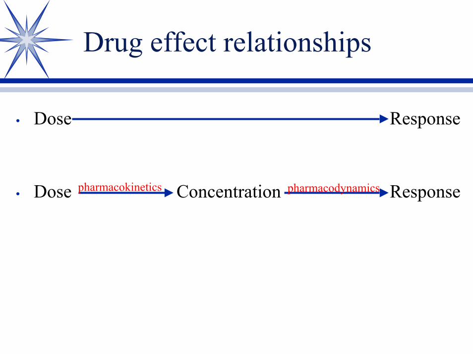
Drug effect relationships

• Dose Response

Res

pons

e

log dose

Res

pons

e

doseHigh variabilitylog concentrationLow variability

Drug effect relationships

• Dose Response

• Dose Concentration Responsepharmacokinetics pharmacodynamics

Pharmacokinetics – Pharmacodynamics(PK – PD)

• If a concentration can be easily measured (blood) and this concentration directly correlates with an effect, then the ability to predict concentrations becomes of therapeutic benefit.

Pharmacokinetics

• Pharmacokinetics (toxicokinetics) is a mathematical description of drug (toxin) disposition in the body. A complete model will address:→absorption (A)→distribution (D)→metabolism (M)→excretion (E)

Types of Pharmacokinetic Modeling

• Data-Based compartmental models(Classical; Compartmental pharmacokinetics)

• Physiologically-Based pharmacokinetic models• Population-Based pharmacokinetic models

• Pharmacokinetic-Pharmacodynamic models

Data-Based Compartmental Pharmacokinetics

• Classic kinetics• Views the body as a series of compartments• Those compartments have a mathematical

volume in which the drug is distributed.• Transfer of drug to and from compartments

is described by rate constants.

Graphical representation

zero-order

first-order

Cartesian semilog

1

10

0 1 2 3 4 5 6 7 8 9 10 11

hours

0

1

2

3

4

56

7

8

9

10

11

0 1 2 3 4 5 6 7 8 9 10 11

hours

01

23

45

67

89

1011

0 1 2 3 4 5 6 7 8 9 10 11

time (hours)

1

1 0

0 2 4 6 8 1 0 1 2

tim e (ho urs )

amou

nt (m

g)

Mixed-order process

d

1.00

10.00

100.00

0 5 10 15

hours

mcg

/ml

Zero-order

First-order

Transitional

Semi-log plot of first-order one-compartment model

1

dose

k10=λ

Vc

1

10

0 1 2 3 4 5 6 7 8 9 10 11

hours

C = C0 • e-λt

Slope (λ) is a proportion/time i.e., /hr or hr-1

Two compartment model

1

10

0 1 2 3 4 5 6 7 8 9 10 11

hours

mcg

/ml

• Some drug plasma concentration-time profiles are biphasic.

Distribution phase

Elimination phase

Method of residuals (feathering or curve stripping)

0.1

1

10

100

0 5 10 15 20

hr

mcg

/ml Slope = λz

y-intercept = CzC = (C1 • e-λ1t ) + (Cz • e-λzt)

Method of residuals (feathering or curve stripping)

0.1

1.0

10.0

100.0

0 5 10 15 20hr

mcg

/ml

λ1

C = (C1 • e-λ1t ) + (Cz • e-λzt)C1

Microconstants

• k12, k21, k10 etc. are “microconstants• To calculate microconstants:

→1st step: k21 = C1•λz + Cz • λ1C1 + Cz

→2nd step: k10 = λ1 • λz

k21→3rd step: k12 = λ1 + λz - k21 - k10

Two-compartment model

dose

k12

1 2k21Vc Vp

k10

Three-compartment model

1

10

0 1 2 3 4 5 6 7 8 9 10 11

hours

mcg

/ml

days

• Equation→C = (C1 • e-λ1t ) + (C2 • e-λ2t) + (Cz • e-λzt)

Three-compartment model

dose

1 2k12k13

3 k21k31

k10

Three-compartment model

• Compartment #1→central compartment→blood, extracellular fluid, highly perfused

tissues• Compartment #2

→less perfused tissues; e.g., muscle• Compartment #3

→deep compartment→poorly perfused tissue; e.g., fat, bone

Physiologic-based pharmacokinetics

• Compartments correspond to anatomical spaces so that physiologic interactions can be incorporated into the model.

• Allows extrapolation outside the range of data to deal with altered physiology (disease states).

Physiologic pharmacokinetics

• Model may incorporate these factors→anatomic

organ volume

→physiologicblood flow chemical reactions

→transport membrane permeabilities

→thermodynamic protein or tissue binding

Physiologic approach to clearance

Eliminationorgan

• CL = Q(ER)• ER = (Ca - Cv) / Ca• CL = Q [ (Ca - Cv) / Ca ]

Eliminateddrug

Q • Ca Q • Cv

Rate of exit from the rumen

Dose theophylline Dose Cr-EDTA

4 6Vr Vcr

k40 k60

k41

k14

Computer programs

• Most programs can be used, but WINNONLIN and Advanced Continuous Simulation Language (ACSL) are commonly employed software programs

Population pharmacokineticsReference: JVPT 21(3), 167-189, 1998.

• Traditional kinetic studies usually conducted in small number of healthy individuals

• How to account for disease effects and differences in population→therapeutic drug monitoring→physiologic kinetics→population kinetics

Population pharmacokinetics

• Compartmental and physiologic kinetics derive their information from extensive sampling of a small number of animals, usually in good health.

• Population kinetics derive their information from limited sampling of a much larger number of animals, often representing the target population (diseased animals).

Population pharmacokinetics

• Population kinetics identify surrogate parameters (age, body weight, common clinical test results) as covariates that relate the physiologic factors altering the underlying pharmacokinetic model. → e.g., age → % body water → volume of distribution

Cr clearance → GFR → CL• “In other words, one must determine the sources of

pharmacokinetic variability in a patient population as well as the magnitude of that variability, in order to design dosage regimens that account for individual patient characteristics.”

Pharmacostatistical Model

Structural ModelCi = D / Vd • e- CL / Vd • t

•Fixed effectsdosetime

•Fixed-effect parameters

clearancevolume of

distribution

Regression ModelClavg = θ1 + (θ2 • CRCL)Vdavg = θ3 +(θ4 • Age)

•Fixed effectsagecreatinine clearance

•Fixed-effect parametersθ1, θ2, ... θn

Statistical Model•Intraindividual random effects

Cij = Ci + εij•Intraind. random-effect parameter

σ2 (variance of ε)•Interindividual random effects

CLj = CLavg + ηCLjVdj = Vdavg + ηVdj

•Interind. random-effect parameters

ω2CL (variance of ηCL)ω2Vd (variance of ηVd)

Pharmacokinetic model(Fixed Effects)

Statistical Model(Random Effects)

Types of true population pharmacokinetic methods

• Parametric→assumes a normal or log-normal distribution→usually simpler; computer program NONMEM

• Nonparametric→does not require a normal distribution and can identify

deviations such as bimodal or skewed distributions→computes a “joint probability density function’, which

measures the variance of two parameters and how they are related

→Computer programs NPEM, NPML, and NPAG (part of USC-PACK)

Pharmacokinetic model only

Population modelIncludes age, CrCL, and body wt as covariates

Population pharmacokinetic methods

• More representative of the population to which the drug is targeted.

• Requires less rigid experimental design.• Less extensive sampling per subject creating less

patient stress.

‘True’ population pharmacokinetic methods

• Characterizes random effects including both inter- and intraindividual (residual) variability of the estimated parameters.

• Allows not only for the prediction of the effect of clinical features on kinetic parameters, but the degree of confidence in those predictions.

PK – Pharmacodynamic models

•When hysteresis occurs in the time-concentration profile versus the time-effect profile, a PK-PD model should be developed.

All figures from: “Riviere, J. E. Comparative pharmacokinetics : principles, techniques, and applications; Ames, : Iowa State University press, 1999.

PK-Pharmacodynamic models

Effector compartment

PK-Pharmacodynamic models

Reflects barriers between the central compartment and the receptors and is

a function of anatomical location, blood perfusion, and tissue

permeabilities.

Hill equation often used to describe concentration-effect relationship

γ determines slope of sigmoid C-E curve; related to drug-receptor binding ratio

PK-PD model of meperidine in goats

Validation of meperidine model

PB-PK-PD models

• Some models have been created for toxicology risk assessment using ACSL.

• Example: “A Physiologically Based Pharmacokinetic and Pharmacodynamic Model of Paraoxon in Rainbow Trout. Toxicology & Applied Pharm 145, 1997, 192-201”

• Used “Continuous System Modeling Program III (CSMP III) software

A

R

T

E

R

Y

V

E

I

N

Brain

Heart

Liver

Muscle

Kidney

QBr

QH

QL

QM

QK

QM • 0.6

E

WaterPB-PK modelCLD CLu

GillCv Ca

PD model ofcholinesterase inactivation

Paraoxon

AChE

RO

+

KAChE [PO + AChE]

KD

CaE [PO + CaE]RO

+KCaE

KD

AChE-1 = (KAChE/Ri) [paraoxon] + KD/Ro

Parameters Used in the Model

• Paraoxon conc.• AChE conc.• CaE conc.• Tissue/plasma partition coeff.• Brain AChE synthesis rate• Brain AChE degradation rate• Blood flow to each tissue• Tissue volume

• AChE bimolecular rate constant

• CaE bimolecular rate constant

• Hepatic clearance• Water uptake clearance• Water depuration

clearance

Model-predicted AChE activity after water exposure to 75 ng/ml paraoxon

• exp. data point…. predicted conc; model w/o CaE predicted conc; model w/ CaE

Table 3Sensitivity of Brain AChE Inhibition to Changes

in the PBPK-PD Model Parameters

CaE bimolecular rate constant

AChE bimolecular rate

constant

Hepatic clearance

Brain AChE degradation rate

Brain AChE synthesis rate

Tissue/plasmaPartition coeff.

Blood flow

Carboxylesterase conc.

AChE conc +1.0[AChE]+1.8[CaE]

+2.8KCaE

-3.0KAChE

<0.1CLh

-1.5KD

+17.9Ro

<0.1R-0.8Q

Percent change in brain AChE inhibitionwhen model parameter is increased 10%Parameter

PK-PD Modeling

• Quantitatively describe the mechanisms affecting drug disposition

• Allows the prediction of what a change in drug dosage, population variabilty, a physiolgic change, or a disease effect will have on the response of a patient or patient population.

Mathematical approaches to modeling (Computer modeling)

• Linear (least squares) regression and curve stripping

• Nonlinear regression• MAP Bayesian • Nonparametric

Linear regression and curve stripping

• Advantages→ Simple; used before computers readily available

• Disadvantages→ Requires transformation of data to obtain linearity using

ln(concentration)→ Can only fit single-dose data→ Emphasizes lower concentrations

Relative weights by linear regression proportional to the reciprocal of their squarese.g., 8.0 and 1.5 mcg/ml; weight 82 / 1.52 = (1/64)/(1/2.25) = 28.4 times more emphasis given to 1.5 compared to 8.0 mcg/ml

Nonlinear regression

• Advantages→ Designed to fit data to a curve, so no data transformation is

necessary→ Can fit data from multi-dose profile→ Can provide correct weighting to the data based on its

credibility (Fisher information)

• Disadvantages→ Requires at least one serum concentration for each

parameter to be fitted→ Does not take into account covariants from the population.

(To be discussed in Population Kinetics approaches)

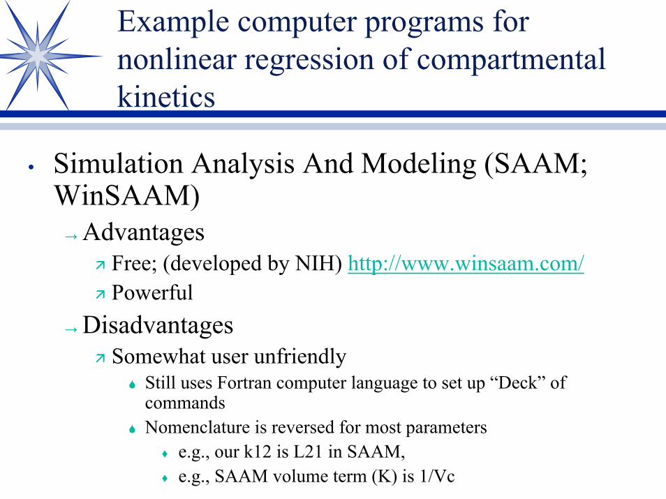
Example computer programs for nonlinear regression of compartmental kinetics

• Simulation Analysis And Modeling (SAAM; WinSAAM)→Advantages

Free; (developed by NIH) http://www.winsaam.com/Powerful

→DisadvantagesSomewhat user unfriendly

Still uses Fortran computer language to set up “Deck” of commandsNomenclature is reversed for most parameters

♦ e.g., our k12 is L21 in SAAM, ♦ e.g., SAAM volume term (K) is 1/Vc

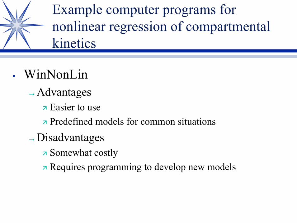
Example computer programs for nonlinear regression of compartmental kinetics

• WinNonLin→Advantages

Easier to usePredefined models for common situations

→DisadvantagesSomewhat costlyRequires programming to develop new models

MAP Bayesian Fitting

• Bayes Theorem quantitatively describes relationships between → Existing probabilities→ New information→ Predicts revised (posterior) probabilities

• These revised probabilities are referred to as Maximum Aposteriori Probability (MAP)

• Typically employed in population kinetic modeling (to be discussed), it also fits compartmental parameters

MAP Bayesian Fitting

• Pros→Same benefits as nonlinear fitting AND→Adds estimates of parameter variability into the

model→Adds population data and its variability into the

model→Can fit with only one data point per subject

MAP Bayesian Fitting

• Cons→ More complicated models and software→ Unable to separate inter- from intra-individual subject

variability.→ A parametric approach, it assumes normal or log-normal

distributions• Common software

→ NonMemThe standard. A commercial product $

→ USC-PAKIncreasingly used. Free (USC) but requires commercial Fortran compiler $

Nonparametric approaches

• Regarded by many as the preferred approach• Pros

→ Makes no assumptions about the distribution of the population parameter (can discover bimodal distributions and subpopulations such as “fast versus slow acetylators”

• Cons→ Computer intensive. Most require the use of a

supercomputer. Common Software:→ NPLM (nonparametric maximum likelihood method)→ NPEM (nonparametric expectation-maximization method)→ NPAG (nonparametric adaptive grid; recently moved to

microcomputer)