PHAR 7632 Chapter TWO - Boomer · PHAR 7632 Chapter TWO 02/02/2006 10:46 PM Page 4 of 28 PHAR 7632 Chapter 2 Background Mathematical Material

02/02/2006 10:46 PMPHAR 7632 Chapter TWO

Page 1 of 28http://www.boomer.org/c/p4/c02/c02.html

PHAR 7632 Chapter 2

Background Mathematical Materialreturn to the Course index

previous | next

Student Objectives for this Chapter

After completing the material in this chapter each student should:-

understand exponents and logarithms, algebraically and graphicallybe able to use linear (Cartesian) and semi-log graph paper for the representation of databe able to draw a 'best-fit' straight line through data on linear and semi-log graph paperunderstand and able to use spreadsheetsunderstand differential and integral calculusbe able to write differential equations given a compartmental modeling scheme as a diagram or descriptionbe able calculate the area under the plasma concentration versus time curve (AUC) using the linear trapezoidal rule

return to the Course index previous | next

This page was last modified: Saturday 31 Dec 2005 at 03:50 PM

Material on this website should only be used for Educational or Self-Study Purposes

Copyright 2001-2006 David W. A. Bourne ([email protected])



PHAR 7632 Chapter 2


previous | next

ExponentsDefinition:

N = bx or N = b^x or N = b ** x

where N is the number, b is the base, often 10 but also e ( = 2.7183... Napier's constant), and x is the exponent (or power term whenan integer as in 102 is 10 to the power 2).

Note use of ^ (common calculator or single line format) or ** (common computer language format)

With the same base, exponents can be added or subtracted

For example; ax x ay = a(x+y) to perform multiplication

or

ax / ay = a(x-y) to perform division.

Some Example Calculations

a) 100 = 102 = 10^2 = 10**2

b) 100 = e4.605 = e^4.605 = e**4.605 where e = 2.7183 !!!

c) 10 x 100 = 101 x 102 = 101+2 = 103 = 1000

d) 10 x 100 = e2.303 x e4.605 = e6.908 = 1000 when the base is the same you can add exponents to multiply numbers

Subtract exponents to divide

e) 5.6/1.2 = e1.723 / e0.182 = e1.723 - 0.182 = e1.541 = 4.67

Use your calculator to check this answer

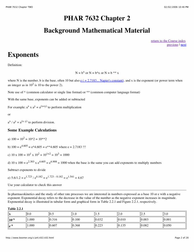
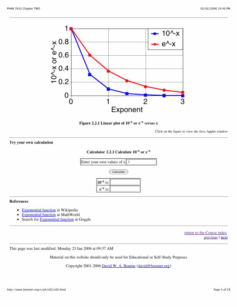
In pharmacokinetics and the study of other rate processes we are interested in numbers expressed as a base 10 or e with a negativeexponent. Exponential decay refers to the decrease in the value of the number as the negative exponent increases in magnitude.Exponential decay is illustrated in tabular form and graphical form in Table 2.2.1 and Figure 2.2.1, respectively.

Table 2.2.1 x 0.0 0.5 1.0 1.5 2.0 2.5 3.0

10-x 1.000 0.316 0.100 0.032 0.010 0.003 0.001

e-x 1.000 0.607 0.368 0.223 0.135 0.082 0.050



Figure 2.2.1 Linear plot of 10-x or e-x versus x

Click on the figure to view the Java Applet window

Try your own calculation

Calculator 2.2.1 Calculate 10-x or e-x

Enter your own values of x 1

Calculate

10-x is:

e-x is:

References

Exponential function at WikipediaExponential function at MathWorldSearch for Exponential function at Goggle


This page was last modified: Monday 23 Jan 2006 at 09:37 AM





PHAR 7632 Chapter 2


previous | next

LogarithmsIf N = bx then x = logb N

For example, 100 = 102 thus log (100) = 2 [base 10 assumed] or 100 is the antilog of 2.

These are called common logs (log). Natural logs (ln) use the base e (=2.7183). Note the use of log and ln to denote common ornatural logarithms, respectively.

To convert from common log (base 10) to natural log (base e)

use 2.303 x log10(N) = lne(N)

that is, ln(10) x log(N) = ln(N)

For example, ln (100) = 2.303 x log (100) = 2.303 x 2 = 4.606

Common logs are often used with equilibrium equations and buffer or pH calculations. Logarithms to base e are often used inpharmacokinetics and other kinetic processes.

Before calculators, logarithms were used to multiply or divide numbers. The two numbers to be multiplied or divided would beconverted to logarithms. For multiplication the logs are added and for division the logs are subtracted.

Examples: a) 23.7 x 56.4 = x

To find x take the natural log of both numbers, add and take the 'anti'-log (base e)

ln(23.7) + ln(56.4) = ln(x)

3.1655 + 4.0325 = 7.1980 = ln(x)

x = 1337

or 23.7 x 56.4 = e3.1655 x e4.0325 = e(3.1655 + 4.0325) = e7.1980 = 1337

b) 6.75 / 14.7 = y

To find y take the common log of both numbers, subtract and take the 'anti'-log (base 10)

log(6.75) - log(14.7) = log(y)

0.8293 - 1.1673 = -0.338 = log(y)

y = 0.4592



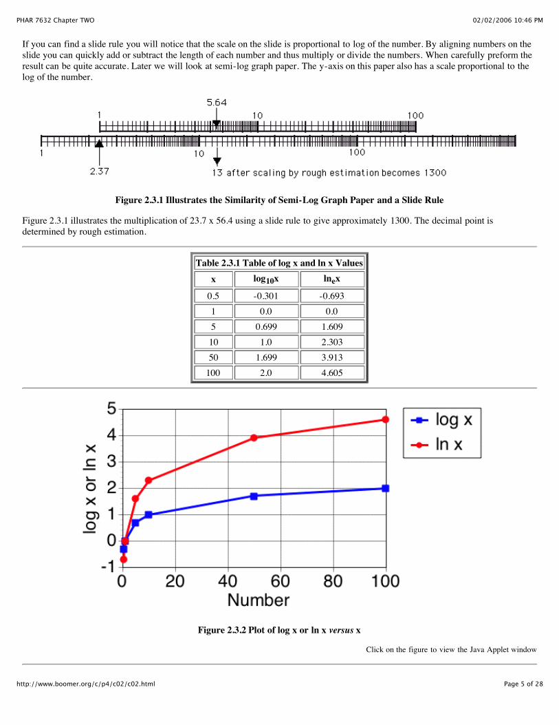
If you can find a slide rule you will notice that the scale on the slide is proportional to log of the number. By aligning numbers on theslide you can quickly add or subtract the length of each number and thus multiply or divide the numbers. When carefully preform theresult can be quite accurate. Later we will look at semi-log graph paper. The y-axis on this paper also has a scale proportional to thelog of the number.

Figure 2.3.1 Illustrates the Similarity of Semi-Log Graph Paper and a Slide Rule

Figure 2.3.1 illustrates the multiplication of 23.7 x 56.4 using a slide rule to give approximately 1300. The decimal point isdetermined by rough estimation.

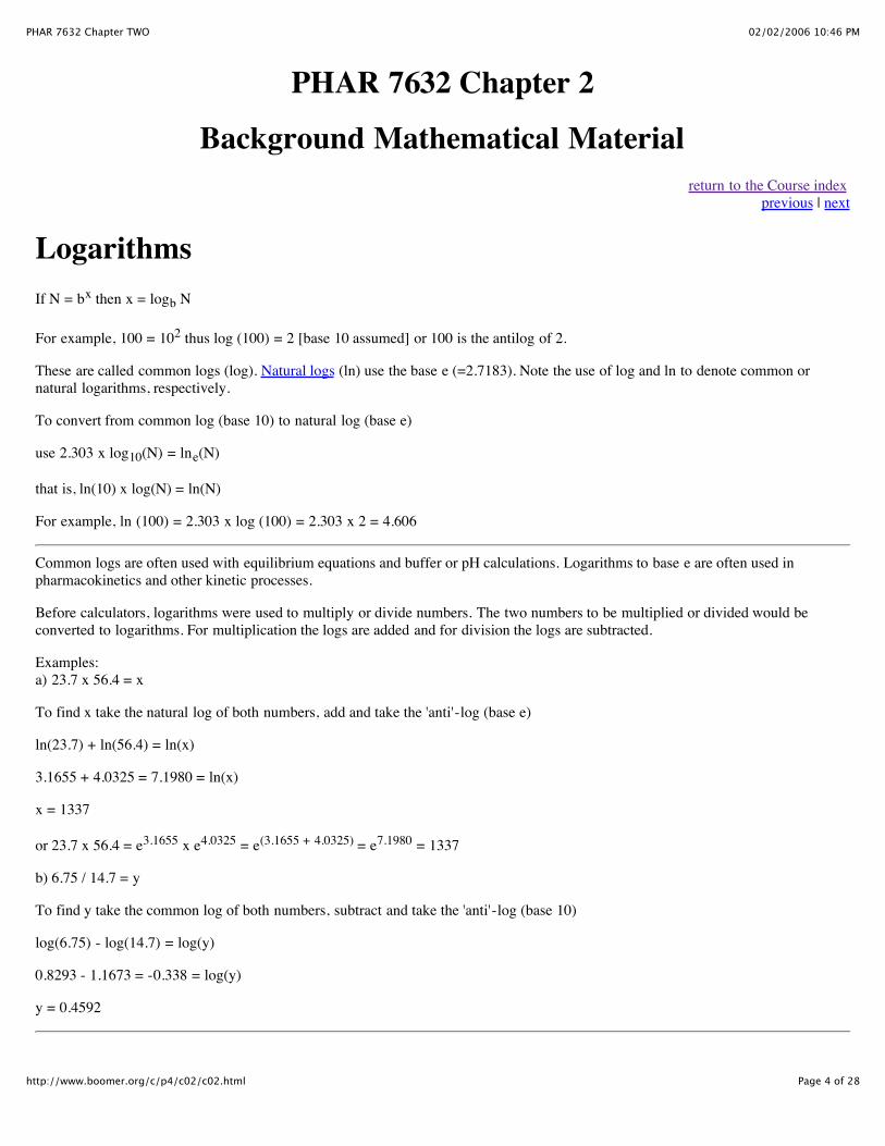
Table 2.3.1 Table of log x and ln x Valuesx log10x lnex

0.5 -0.301 -0.6931 0.0 0.05 0.699 1.60910 1.0 2.30350 1.699 3.913

100 2.0 4.605

Figure 2.3.2 Plot of log x or ln x versus x




References

Logarithm at WikipediaSearch for Logarithm at GoggleSearch for Slide Rule at Goggle


This page (http://www.boomer.org/c/p4/c02/c0203.html) was last modified: Saturday 31 Dec 2005 at 03:50 PM





PHAR 7632 Chapter 2


previous | next

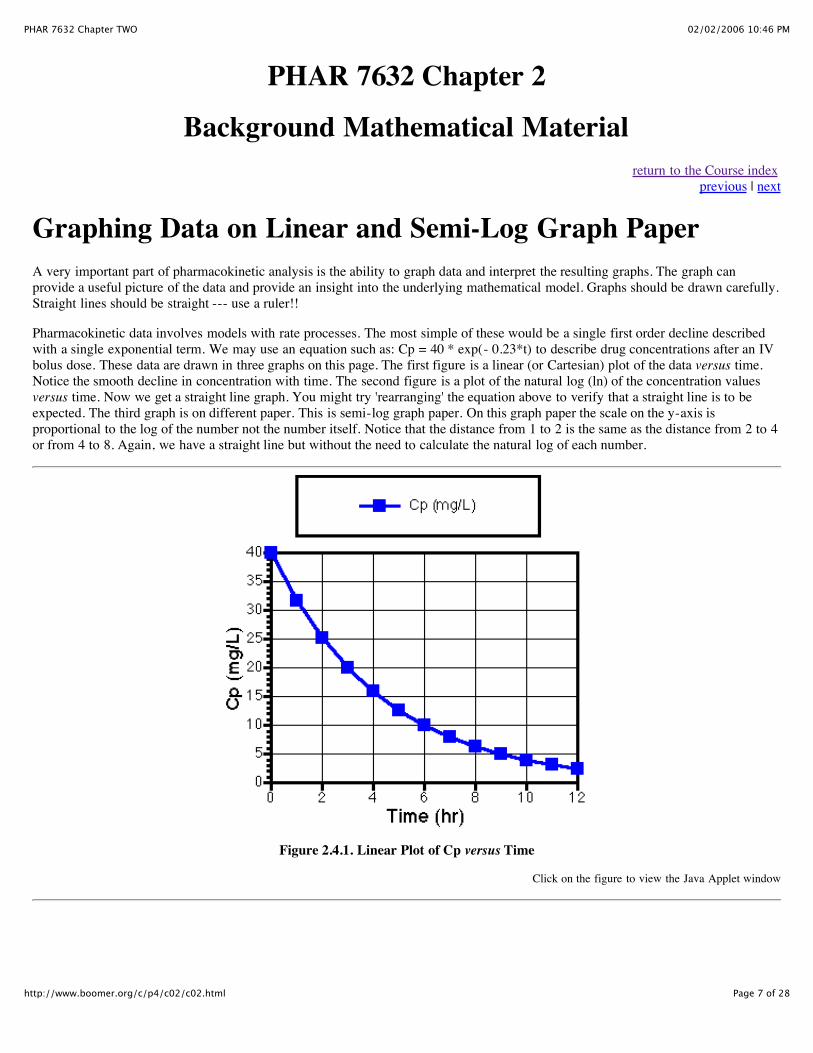
Graphing Data on Linear and Semi-Log Graph PaperA very important part of pharmacokinetic analysis is the ability to graph data and interpret the resulting graphs. The graph canprovide a useful picture of the data and provide an insight into the underlying mathematical model. Graphs should be drawn carefully.Straight lines should be straight --- use a ruler!!

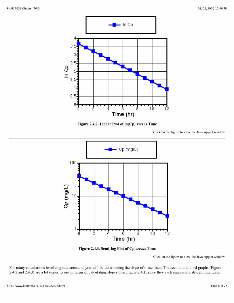
Pharmacokinetic data involves models with rate processes. The most simple of these would be a single first order decline describedwith a single exponential term. We may use an equation such as: Cp = 40 * exp(- 0.23*t) to describe drug concentrations after an IVbolus dose. These data are drawn in three graphs on this page. The first figure is a linear (or Cartesian) plot of the data versus time.Notice the smooth decline in concentration with time. The second figure is a plot of the natural log (ln) of the concentration valuesversus time. Now we get a straight line graph. You might try 'rearranging' the equation above to verify that a straight line is to beexpected. The third graph is on different paper. This is semi-log graph paper. On this graph paper the scale on the y-axis isproportional to the log of the number not the number itself. Notice that the distance from 1 to 2 is the same as the distance from 2 to 4or from 4 to 8. Again, we have a straight line but without the need to calculate the natural log of each number.

Figure 2.4.1. Linear Plot of Cp versus Time




Figure 2.4.2. Linear Plot of ln(Cp) versus Time


Figure 2.4.3. Semi-log Plot of Cp versus Time


For many calculations involving rate constants you will be determining the slope of these lines. The second and third graphs (Figure2.4.2 and 2.4.3) are a lot easier to use in terms of calculating slopes than Figure 2.4.1, since they each represent a straight line. Later



we will revisit the equation for this line. Remember semi-log graph paper has a normal x- axis scaling but the y- axis scaling isproportional to the log of the number not the number itself. It saves you from taking the log of each number before you plot it. Note:Once you take the log of a number you loose the units.

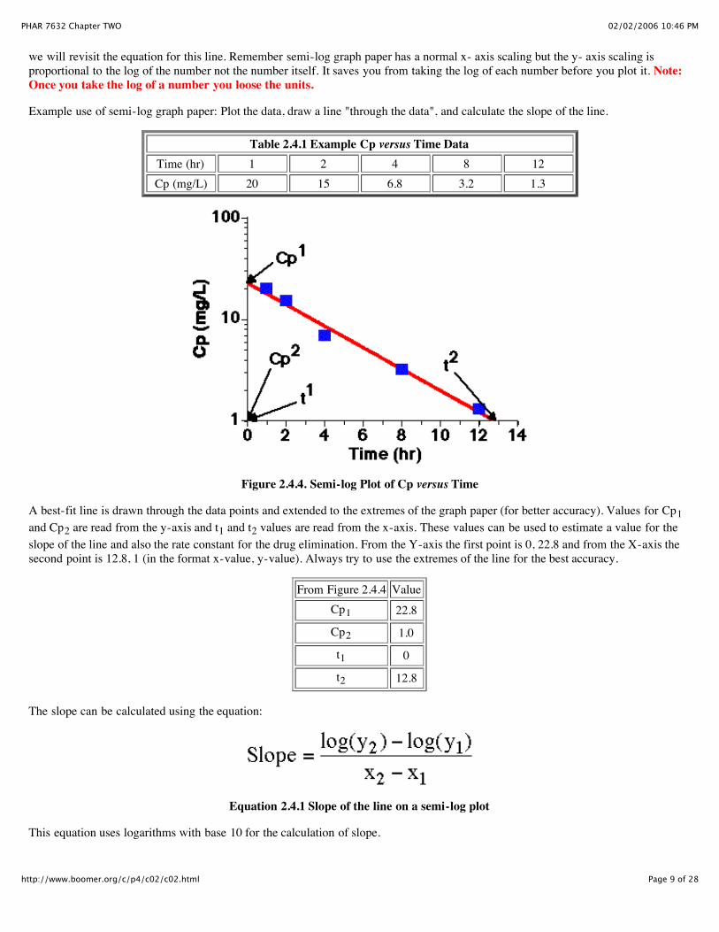
Example use of semi-log graph paper: Plot the data, draw a line "through the data", and calculate the slope of the line.

Table 2.4.1 Example Cp versus Time DataTime (hr) 1 2 4 8 12Cp (mg/L) 20 15 6.8 3.2 1.3

Figure 2.4.4. Semi-log Plot of Cp versus Time

A best-fit line is drawn through the data points and extended to the extremes of the graph paper (for better accuracy). Values for Cp1and Cp2 are read from the y-axis and t1 and t2 values are read from the x-axis. These values can be used to estimate a value for theslope of the line and also the rate constant for the drug elimination. From the Y-axis the first point is 0, 22.8 and from the X-axis thesecond point is 12.8, 1 (in the format x-value, y-value). Always try to use the extremes of the line for the best accuracy.

From Figure 2.4.4 ValueCp1 22.8

Cp2 1.0

t1 0

t2 12.8

The slope can be calculated using the equation:

Equation 2.4.1 Slope of the line on a semi-log plot

This equation uses logarithms with base 10 for the calculation of slope.



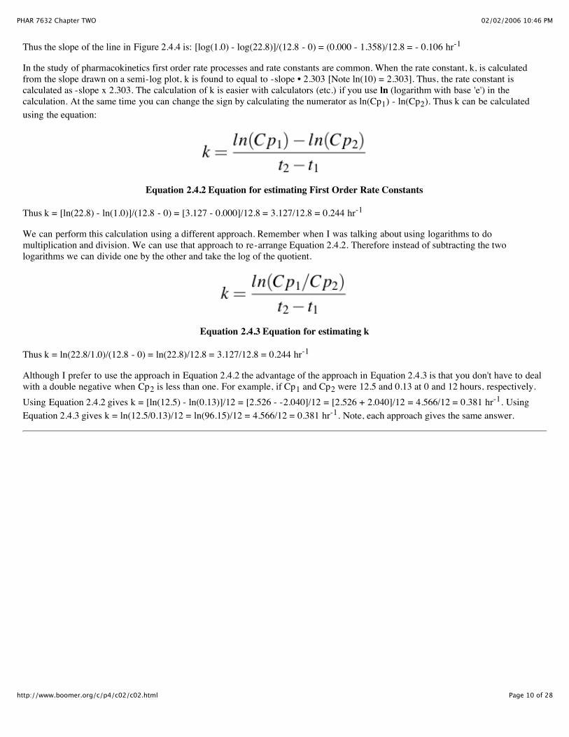
Thus the slope of the line in Figure 2.4.4 is: [log(1.0) - log(22.8)]/(12.8 - 0) = (0.000 - 1.358)/12.8 = - 0.106 hr-1

In the study of pharmacokinetics first order rate processes and rate constants are common. When the rate constant, k, is calculatedfrom the slope drawn on a semi-log plot, k is found to equal to -slope • 2.303 [Note ln(10) = 2.303]. Thus, the rate constant iscalculated as -slope x 2.303. The calculation of k is easier with calculators (etc.) if you use ln (logarithm with base 'e') in thecalculation. At the same time you can change the sign by calculating the numerator as ln(Cp1) - ln(Cp2). Thus k can be calculatedusing the equation:

Equation 2.4.2 Equation for estimating First Order Rate Constants

Thus k = [ln(22.8) - ln(1.0)]/(12.8 - 0) = [3.127 - 0.000]/12.8 = 3.127/12.8 = 0.244 hr-1

We can perform this calculation using a different approach. Remember when I was talking about using logarithms to domultiplication and division. We can use that approach to re-arrange Equation 2.4.2. Therefore instead of subtracting the twologarithms we can divide one by the other and take the log of the quotient.

Equation 2.4.3 Equation for estimating k

Thus k = ln(22.8/1.0)/(12.8 - 0) = ln(22.8)/12.8 = 3.127/12.8 = 0.244 hr-1

Although I prefer to use the approach in Equation 2.4.2 the advantage of the approach in Equation 2.4.3 is that you don't have to dealwith a double negative when Cp2 is less than one. For example, if Cp1 and Cp2 were 12.5 and 0.13 at 0 and 12 hours, respectively.Using Equation 2.4.2 gives k = [ln(12.5) - ln(0.13)]/12 = [2.526 - -2.040]/12 = [2.526 + 2.040]/12 = 4.566/12 = 0.381 hr-1. UsingEquation 2.4.3 gives k = ln(12.5/0.13)/12 = ln(96.15)/12 = 4.566/12 = 0.381 hr-1. Note, each approach gives the same answer.



Drawing a best-fit line through the Data

Drawing a line through the data doesn't mean through just two data points but through all the data points. Be especially careful aboutpicking two adjacent data points. Sometimes the first and last point can work but the last point, the lowest concentration data pointwill probably be inaccurate. The best approach is to put the line through all the data. There should be points above and below the line.



Calculate kel from the best-fit line

Practice and Assignments

Two exercises allowing you to draw straight lines through data on both linear and on semi-log graph paper.

Linear Graph

Semi-log Graph

Try them out if you need practice graphing data and calculating intercept and slope in these graphs.

Graph Paper Resources

Graph Paper in Adobe Reader (v5.0) - PDF Format. If you have Adobe Reader installed (or Preview in Mac OS X) clicking on thelinks below will provide the graph paper indicated.



Linear 7 x 9 inchesLinear 18 x 22 cm

Semi-log One CycleSemi-log Two CycleSemi-log Three CycleSemi-log Four CycleSemi-log Five Cycle

Video or audio tutorials are available to help with this material

Video PODcast snippets as a RSS Feed for Safari(Mac), or add the URL: http://www.boomer.org/c/snips/phar7632.xml as alive bookmark in Firefox (Mac/Win), or install Sage in Firefox and use the Tools:Sage menu and 'discover' the feed OR Open iTunesand select 'Advanced:Subscribe to Podcast..." then paste in the URL: http://www.boomer.org/c/snips/phar7632.xml


This page (http://www.boomer.org/c/p4/c02/c0204.html) was last modified: Thursday 02 Feb 2006 at 10:48 PM





PHAR 7632 Chapter 2


previous | next

Using SpreadsheetsFrom Visicalc™, to Lotus 1-2-3™, to Excel™, spreadsheets have provided powerful what-if capability to the personal computer user.Using a combination of numbers, labels, and formulas the user is able try out various equations and mathematical scenarios. Theresults of these calculations can be linked to graphical output in various forms of charts or graphs. The spreadsheet program, Excel™

is available for a number of platforms including the Macintosh™ and Windows™ operating systems.

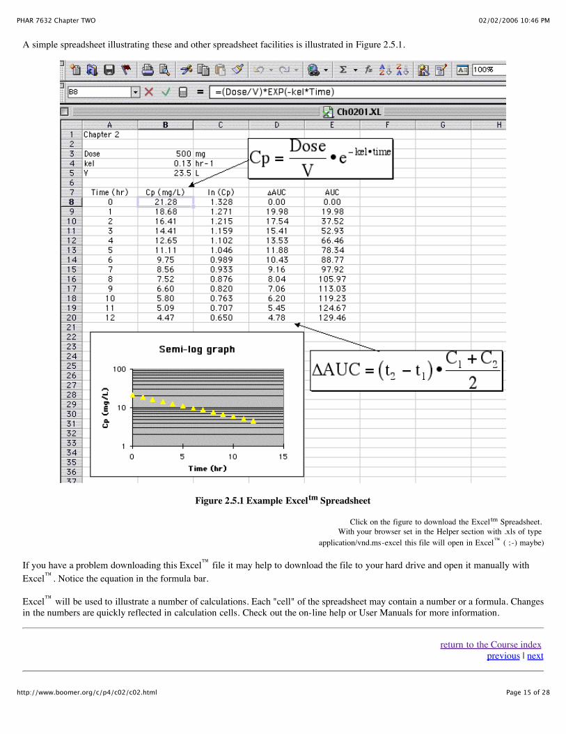
A new spreadsheet document provides a sheet of cells. The user can enter either numbers, labels, or functions into each cell. Cells aredesignated by letter and number. For example, Cell 'A1' in the top left corner contains the text 'Chapter II'. Cells A8:A16 contain thenumbers 0 through 8. Cell B8 could be completed by entering the formula '=($B$3/$B$5)*EXP(-$B$4*A8)' which calculates Cp attime = 0.

Cells with formulas can be copied (down for example) and thus values for Cp at other times can be quickly calculated. Notice the useof '$' to designate absolute cell references. When copied down these references stay the same and refer to the same cell, e.g. B3 =Dose. The reference A8 however is relative and changes for each cell to refer to the relative time in the 'A' column.

Once the formulas are entered changes to parameter values will be quickly reflected by new values in the appropriate cells.



A simple spreadsheet illustrating these and other spreadsheet facilities is illustrated in Figure 2.5.1.

Figure 2.5.1 Example Exceltm Spreadsheet

Click on the figure to download the Exceltm Spreadsheet. With your browser set in the Helper section with .xls of type

application/vnd.ms-excel this file will open in Excel™ ( ;-) maybe)

If you have a problem downloading this Excel™ file it may help to download the file to your hard drive and open it manually withExcel™. Notice the equation in the formula bar.

Excel™ will be used to illustrate a number of calculations. Each "cell" of the spreadsheet may contain a number or a formula. Changesin the numbers are quickly reflected in calculation cells. Check out the on-line help or User Manuals for more information.









PHAR 7632 Chapter 2


previous | next

CalculusDifferential Calculus

Pharmacokinetics is the study of the rate of drug absorption and disposition in the body. Thus differential calculus is an importantstepping stone in the development of many of the equations used. These differential equations can be integrated using a variety oftechniques including Laplace transforms. However, in this course we won't be doing these integrations.

Differential calculus is involved with the study of rates of processes. The calculus part comes in when we look at these processes indetail, that is, during small time intervals.

We may say that at time zero a patient has a concentration of 25 mg/L of a drug in plasma and at time 24 hours the concentration is 5mg/L. That may be interesting in its self, but it doesn't give us any idea of the concentration between 0 and 24 hours, or after 24hours. Using differential calculus we are able to develop equations to look at the process during the small time intervals that make upthe total time interval of 0 to 24 hours. Then we can calculate concentrations at any time after the dose is given.

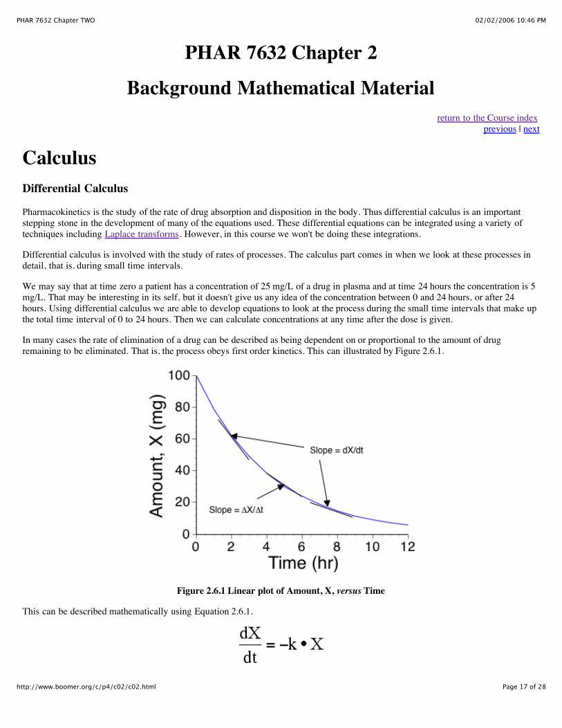
In many cases the rate of elimination of a drug can be described as being dependent on or proportional to the amount of drugremaining to be eliminated. That is, the process obeys first order kinetics. This can illustrated by Figure 2.6.1.

Figure 2.6.1 Linear plot of Amount, X, versus Time

This can be described mathematically using Equation 2.6.1.



Equation 2.6.1. Rate of Change of X with Time

where k is a proportionality constant we call a rate constant and X is the amount remaining to be eliminated. Note the use of thesymbol 'd' to represent a very small increment in X or t. Thus dX/dt represents the slope of the line (or rate of change) over a smallregion of the curved line, see Figure 2.6.1. When data are collected at discrete times such as 4 and 6 hours the larger change in X and tcan be represented by ΔX/Δt as shown in Figure 2.6.1. Note the slope changes as the value of X (y-axis) changes.

Equation 2.6.2. Rate of Elimination

Integration of Equation 2.6.1 (and other differential equations) provides the integrated equations such as Equation 2.6.3.

Equation 2.6.3. Integrated Equation. X versus Time

Equation 2.6.3 is the resulting integrated equation. We will talk more of these equations during the semester.

What we have done is convert the equation for rate of change of X versus time into an equation for X versus time. A differentialequation is converted into an integrated equation. (Compare Equation 2.6.1 and Equation 2.6.3).

We will work with both differential and integrated equations in this course.

Integral Calculus

Differentiation is the reverse of integration. With differentiation breaking a process down to look at the instantaneous process,integration sums up the information from small time intervals to give a total result over a larger time period.

Another example of integration is the calculation of the area under the plasma concentration versus time curve. Later we shall learnthat this summation or integration process can be used to evaluate dosage forms, that is it can be used as a measure of dosage formperformance.

In the section above we converted from the rate of change equation to an equation for X. We can also go further and get an area underthe curve, which is a further integration.

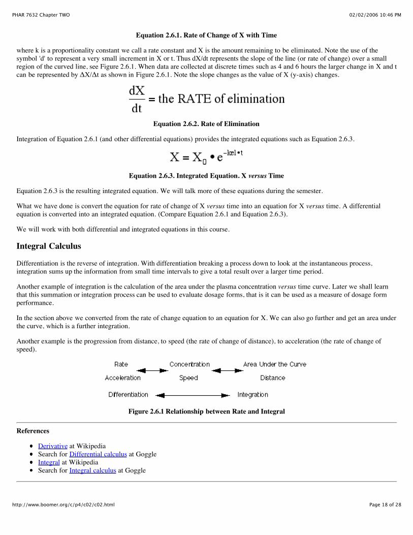
Another example is the progression from distance, to speed (the rate of change of distance), to acceleration (the rate of change ofspeed).

Figure 2.6.1 Relationship between Rate and Integral

References

Derivative at WikipediaSearch for Differential calculus at GoggleIntegral at WikipediaSearch for Integral calculus at Goggle









PHAR 7632 Chapter 2


previous | next

Writing Differential EquationsRate processes in the field of pharmacokinetics are usually limited to first order, zero order and occasionally Michaelis-Mentenkinetics. Linear pharmacokinetic systems consist of first order disposition processes and bolus doses, first order or zero orderabsorption rate processes. These rate processes can be described mathematically.

First Order Equation

Each first order rate process ("arrow") is described by a first order rate constant (k1) and the amount or concentration remaining to betransferred (X1).

Zero Order Equation

Zero order rate processes are described by the rate constant alone. Amount or concentration to the zero power is 1.

Michaelis Menten Equation

The Michaelis Menten process is somewhat more complicated with a maximum rate (velocity, Vm) and a Michaelis constant (Km)and the amount or concentration remaining.

The full differential equation for any component of a pharmacokinetic model can be constructed by adding an equation segment foreach arrow in the pharmacokinetic model. The rules for each segment:

. 1 Direction of the arrowIf the arrow goes into the component the equation segment is positiveIf the arrow leaves the component the equation segment is negative.

. 2 Type of rate processIf the rate process is first order multiply the (first order) rate constant by the amount or concentration of drug in thecomponent at the tail of the arrow.If the process is zero order just enter the rate constant.For a Michaelis Menten processes include the amount or concentration of drug in the component at the tail of the arrowin the Michaelis-Menten equation.



An example

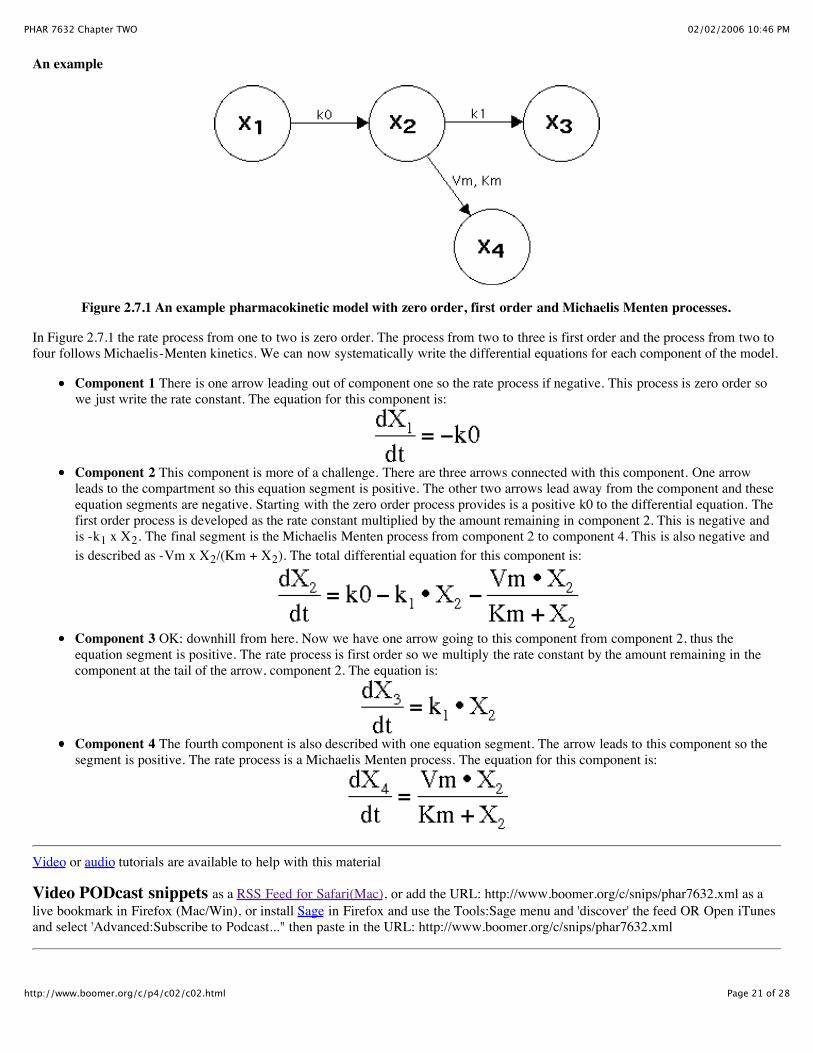
Figure 2.7.1 An example pharmacokinetic model with zero order, first order and Michaelis Menten processes.

In Figure 2.7.1 the rate process from one to two is zero order. The process from two to three is first order and the process from two tofour follows Michaelis-Menten kinetics. We can now systematically write the differential equations for each component of the model.

Component 1 There is one arrow leading out of component one so the rate process if negative. This process is zero order sowe just write the rate constant. The equation for this component is:

Component 2 This component is more of a challenge. There are three arrows connected with this component. One arrowleads to the compartment so this equation segment is positive. The other two arrows lead away from the component and theseequation segments are negative. Starting with the zero order process provides is a positive k0 to the differential equation. Thefirst order process is developed as the rate constant multiplied by the amount remaining in component 2. This is negative andis -k1 x X2. The final segment is the Michaelis Menten process from component 2 to component 4. This is also negative andis described as -Vm x X2/(Km + X2). The total differential equation for this component is:

Component 3 OK; downhill from here. Now we have one arrow going to this component from component 2, thus theequation segment is positive. The rate process is first order so we multiply the rate constant by the amount remaining in thecomponent at the tail of the arrow, component 2. The equation is:

Component 4 The fourth component is also described with one equation segment. The arrow leads to this component so thesegment is positive. The rate process is a Michaelis Menten process. The equation for this component is:






This page was last modified: Friday 06 Jan 2006 at 11:49 AM





PHAR 7632 Chapter 2


previous | next

Area under the plasma concentration time curve (AUC)The area under the plasma (serum, or blood) concentration versus time curve (AUC) has an number of important uses in toxicology,biopharmaceutics and pharmacokinetics.

Toxicology AUC can be used as a measure of drug exposure. It is derived from drug concentration and time so it gives a measurehow much - how long a drug stays in a body. A long, low concentration exposure may be as important as shorter but higherconcentration. Haber's law propose exposure k = C X t (Fritz Haber, 1868-1934) where k is essentially AUC. Some drugs are dosedusing AUC to quantitate the maximum tolerated exposure (AUC Dosing). The efficacy of some antibiotics are related to AUC/MIC,thus maintaining a concentration above a minimum inhibitory concentration (MIC) is more important than peak concentrations.

Biopharmaceutics The AUC measured after administration of a drug product is an important parameter in the comparison of drugproducts. Studies can be performed whereby different drug products may be given to a panel of subject on separate equations. Thesebioequivalency or bioavailability studies can be analyzed by comparing AUC values.

Pharmacokinetics Drug AUC values can be used to determine other pharmacokinetic parameters, such as clearance orbioavailability, F. Similar techniques can be used to calculate area under the first moment curve (AUMC) and thus mean residenttimes (MRT).

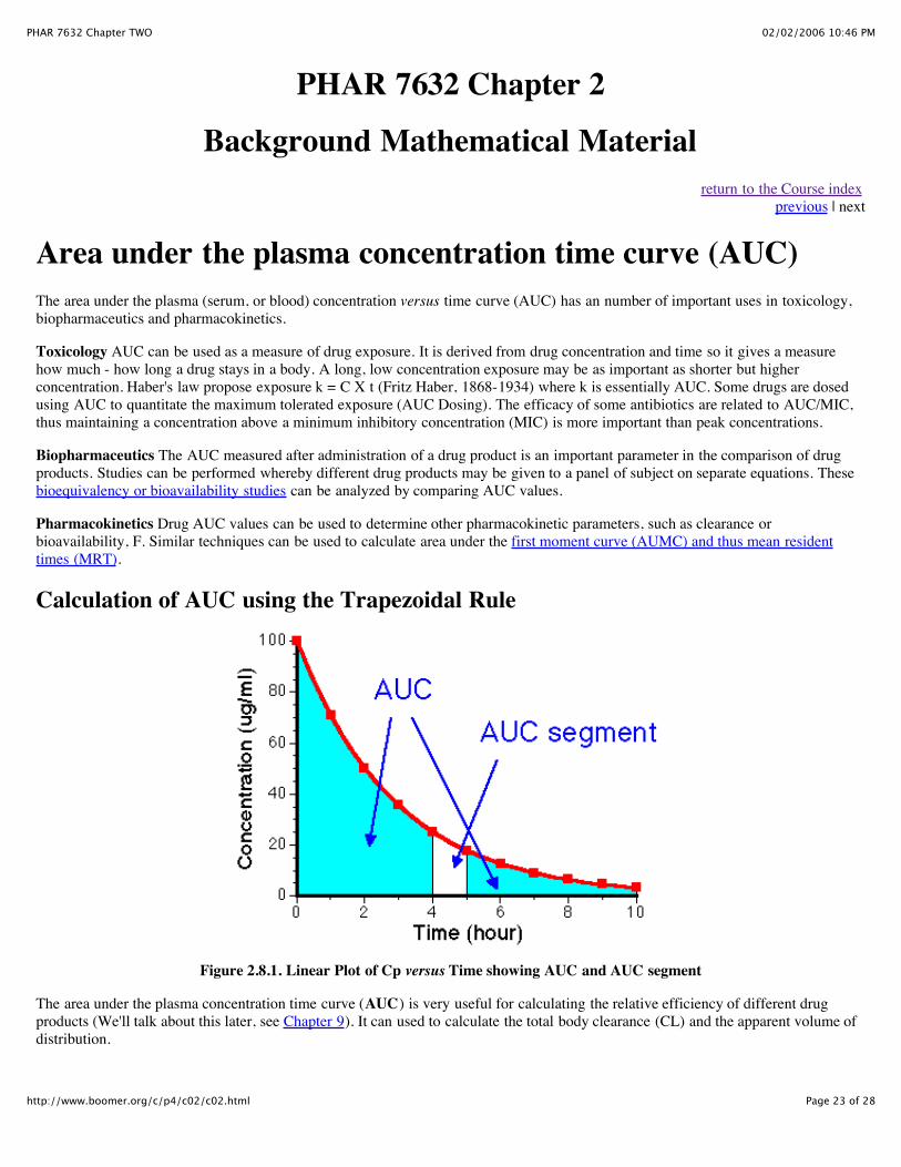
Calculation of AUC using the Trapezoidal Rule

Figure 2.8.1. Linear Plot of Cp versus Time showing AUC and AUC segment

The area under the plasma concentration time curve (AUC) is very useful for calculating the relative efficiency of different drugproducts (We'll talk about this later, see Chapter 9). It can used to calculate the total body clearance (CL) and the apparent volume ofdistribution.



If we have a smooth line for concentration versus time or an equation for Cp versus time from a pharmacokinetic model we couldslice the area into vertical segments. Each segment would be very thin, Δt and in extreme dt, in width (much smaller than the segmentin Fig 2.8.1). The total AUC is calculated by adding these segments together. In calculus this would be the integral. Each very narrowsegment has an area = Cp*dt. Thus the total area (AUC) is given by Equation 2.8.1:

Equation 2.8.1. Total AUC calculated from Very Narrow Segment

Moving ahead a little to Chapter 4 the integrated equation for plasma concentration as a function of time is:

Equation 2.8.2. Cp versus Time after an IV Bolus dose

This is essentially the same as the integrated equation we demonstrated for amount of drug remaining (which can be derived usingLaplace transforms). The difference here is the use of V, apparent volume of distribution, to convert amount into concentration. Wecan substitute this equation for Cpt into Equation 2.8.1 to derive an analytical equation for AUC:

Equation 2.8.3. AUC calculated as the integral of Cp versus time

From Math Tables we would find that:

With a = kel (in Equation 2.8.3), t1 = 0, and t2 = ∞,

At t = 0, e-kel*t = 1 and at t = ∞, e-kel*t = 0

Therefore:

Equation 2.8.4. AUC Calculated from Concentration and kel



This is analytical integration (exact solution, given exact values for V and kel)

Note: For t = 0 to ∞, AUC = Cp0/kel. With t = t to ∞, AUC is calculated as Cpt/kel. We will use this result further down on this page

That is:

Rearranging Equation 2.8.4 to solve for V gives:

V = Dose/(AUC * kel)

Equation 2.8.5. Volume of Distribution Calculated from Dose, AUC and kel

We could use Equation 2.8.4 to calculate the AUC value if we knew DOSE, kel, and V but usually we don't do this. We can calculateAUC directly from the Cp versus time data. We need to use a different approach. The simplest, most common approach is anumerical approximation method called the trapezoidal rule.

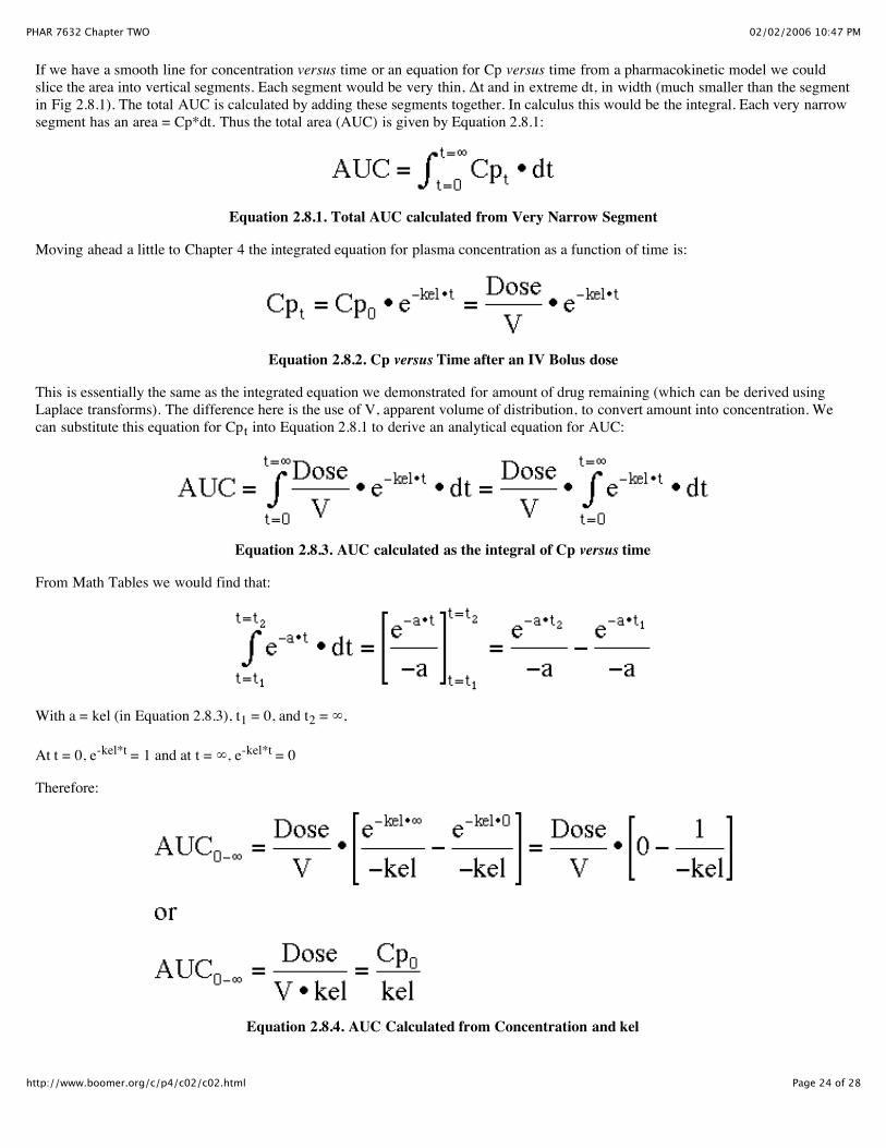
Figure 2.8.2. Linear Plot of Cp versus Time showing Typical Data Points

We can calculate the AUC of each segment if we consider the segments to be trapezoids. [Four sided figure with two parallel sides].

The area of each segment can be calculated by multiplying the average concentration by the segment width. For the segment from Cp2to Cp3:



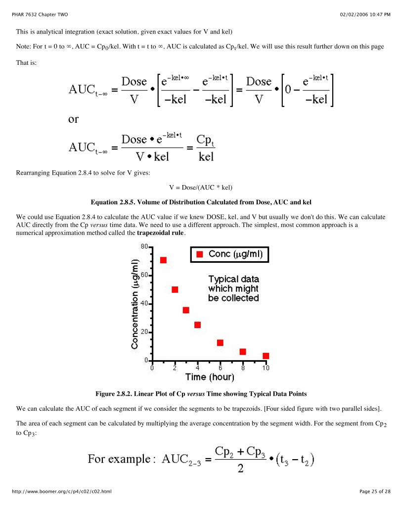
This segment is illustrated in Fig 2.8.3 below.

Figure 2.8.3. Linear Plot of Cp versus Time showing One Trapezoid

The area from the first to last data point can then be calculated by adding the areas together.

Equation 2.8.6 AUC from Cp 1 to Cp n

Note: Summation of data point information (non-calculus)

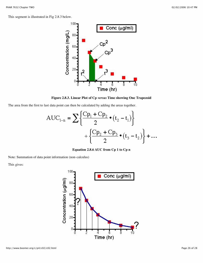
This gives:



Figure 2.8.4. Linear plot of Cp versus time showing areas from data 1 to data n

To finish this calculation we have two more areas to consider. The first and the last segments.

After a rapid IV bolus, the first segment can be calculated after determining the zero plasma concentration Cp0 by extrapolation.

Thus

Equation 2.8.7 AUC from Cp 0 to Cp 1

If we assume that the last data points follow a single exponential decline (a straight line on semi-log graph paper) the final segmentcan be calculated from the equation above from tlast to infinity:

Equation 2.8.8 AUC from tlast to infinity

Thus the total AUC can be calculated as:

Equation 2.8.9 Total AUC from time zero to infinity



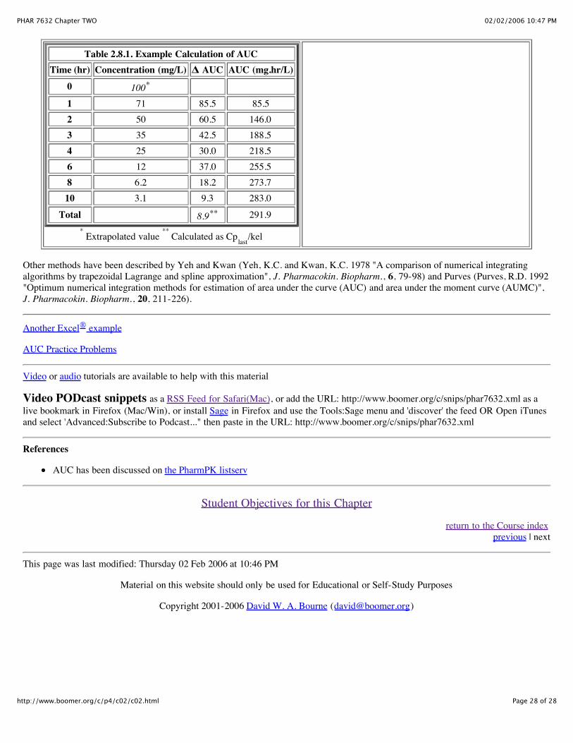
Table 2.8.1. Example Calculation of AUCTime (hr) Concentration (mg/L) Δ AUC AUC (mg.hr/L)

0 100*

1 71 85.5 85.52 50 60.5 146.03 35 42.5 188.54 25 30.0 218.56 12 37.0 255.58 6.2 18.2 273.710 3.1 9.3 283.0

Total 8.9** 291.9* Extrapolated value

** Calculated as Cplast/kel

Other methods have been described by Yeh and Kwan (Yeh, K.C. and Kwan, K.C. 1978 "A comparison of numerical integratingalgorithms by trapezoidal Lagrange and spline approximation", J. Pharmacokin. Biopharm., 6, 79-98) and Purves (Purves, R.D. 1992"Optimum numerical integration methods for estimation of area under the curve (AUC) and area under the moment curve (AUMC)",J. Pharmacokin. Biopharm., 20, 211-226).

Another Excel® example

AUC Practice Problems



References

AUC has been discussed on the PharmPK listserv

Student Objectives for this Chapter


This page was last modified: Thursday 02 Feb 2006 at 10:46 PM



Documents

PHAR 7632 Chapter TWO - Boomer · PHAR 7632 Chapter TWO 02/02/2006 10:46 PM Page 4 of 28 PHAR 7632 Chapter 2 Background Mathematical Material