PH

YS

ICS

LA

B M

AN

UA

L E

NG

INE

ER

ING

SC

IEN

CE

& P

HY

SIC

S D

EP

AR

TM

EN

T

C O L L E G E O F S T A T E N I S L A N D

C I T Y U N I V E R S I T Y O F N E W Y O R K

PHY 114

“The important thing in science is not so much to obtain new facts as to discover new ways of thinking about them.” --Sir William Lawrence Bragg

COLLEGE OF STATEN ISLAND

PHY 114

PHYSICS LAB MANUAL

ENGINEERING SCIENCE & PHYSICS DEPARTMENT

CITY UNIVERSITY OF NEW YORK

ENGINEERING SCIENCE & PHYSICS DEPARTMENT

PHYSICS LABORATORY EXT 2978, 4N-214/4N-215

ENGINEERING SCIENCE & PHYSICS DEPARTMENT

PHYSICS LABORATORY EXT 2978, 4N-214/4N-215

LABORATORY RULES

1. No eating or drinking in the laboratory premises.

2. The use of cell phones is not permitted.

3. Computers are for experiment use only. No web surfing, reading e-mail,

instant messaging or computer games allowed.

4. When finished using a computer log-off and put your keyboard and mouse

away.

5. Arrive on time otherwise equipment on your station will be removed.

6. Bring a scientific calculator for each laboratory session.

7. Have a hard copy of your laboratory report ready to submit before you enter

the laboratory.

8. Some equipment will be required to be signed out and checked back in. The

rest of the equipment should be returned as directed by the technician. All

equipment must be treated with care and caution. No markings or writing is

allowed on any piece of equipment or tables. Remember, you are responsible

for the equipment you use during an experiment.

9. After completing the experiment and, if needed, putting away equipment,

check that your station is clean and clutter free and push in your chair.

10. Before leaving the laboratory premises, make sure that you have all your

belongings with you. The lab is not responsible for any lost items.

Your cooperation in abiding by these rules will be highly appreciated.

Thank You.

The Physics Laboratory Staff

ENGINEERING SCIENCE & PHYSICS DEPARTMENT

PHYSICS LABORATORY EXT 2978, 4N-214/4N-215

10 ESSENTIALS of

writing laboratory reports ALL students must comply with

1. No report is accepted from a student who didn’t actually participate in the

experiment.

2. Despite that the actual lab is performed in a group, a report must be individually

written. Photocopies or plagiaristic reports will not be accepted and zero grade

will be issued to all parties.

3. The laboratory report should have a title page giving the name and number of

the experiment, the student's name, the class, and the date of the experiment.

The laboratory partner’s name must be included on the title page, and it should

be clearly indicated who the author and who the partner is.

4. Each section of the report, that is, “objective”, “theory background”, etc.,

should be clearly labeled. The data sheet collected by the author of the report

during the lab session with instructor’s signature must be included – no report

without such a data sheet indicating that the author has actually performed the

experiment is to be accepted.

5. Paper should be 8 ½” x 11”. Write on one side only using word-processing

software. Ruler and compass should be used for diagrams. Computer graphing

is also accepted.

6. Reports should be stapled together.

7. Be as neat as possible in order to facilitate reading your report.

8. Reports are due one week following the experiment. No reports will be

accepted after the "Due-date" without penalty as determined by the instructor.

9. No student can pass the course unless he or she has turned in a set of laboratory

reports required by the instructor.

10. The student is responsible for any further instruction given by the instructor.

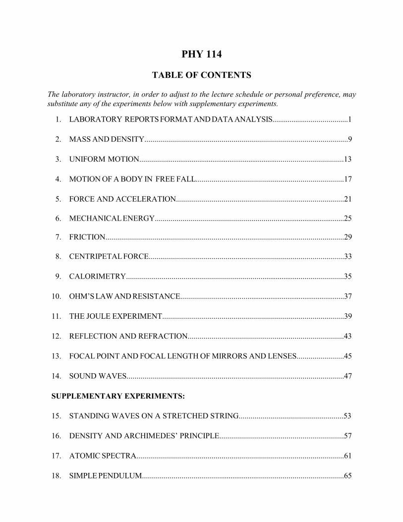
PHY 114

TABLE OF CONTENTS

The laboratory instructor, in order to adjust to the lecture schedule or personal preference, maysubstitute any of the experiments below with supplementary experiments.

1. LABORATORY REPORTS FORMAT AND DATA ANALYSIS.......................................1

2. MASS AND DENSITY.......................................................................................................9

3. UNIFORM MOTION..........................................................................................................13

4. MOTION OF A BODY IN FREE FALL...........................................................................17

5. FORCE AND ACCELERATION.....................................................................................21

6. MECHANICAL ENERGY.................................................................................................25

7. FRICTION.........................................................................................................................29

8. CENTRIPETAL FORCE...................................................................................................33

9. CALORIMETRY...............................................................................................................35

10. OHM’S LAW AND RESISTANCE.....................................................................................37

11. THE JOULE EXPERIMENT............................................................................................39

12. REFLECTION AND REFRACTION...............................................................................43

13. FOCAL POINT AND FOCAL LENGTH OF MIRRORS AND LENSES........................45

14. SOUND WAVES..............................................................................................................47

SUPPLEMENTARY EXPERIMENTS:

15. STANDING WAVES ON A STRETCHED STRING.....................................................53

16. DENSITY AND ARCHIMEDES’ PRINCIPLE...............................................................57

17. ATOMIC SPECTRA.........................................................................................................61

18. SIMPLE PENDULUM.......................................................................................................65

19. VERNIER CALIPER - MICROMETER CALIPER.........................................................67

20. EQUILIBRIUM OF A RIGID BODY................................................................................73

21. ACCELERATION.............................................................................................................79

22. FOCAL LENGTH OF A CONVERGING LENS............................................................83

APPENDIX:

A1 GRAPHICAL ANALYSIS 3.4 - FINDING THE BEST..................................................89

A2 TECHNICAL NOTES ON VERNIER LABQUEST2 INTERFACE...............................93

A3 TECHNICAL NOTES ON SENSORS AND PROBES...................................................97

A4 MULTIMETERS AND POWER SUPPLIES.................................................................103

All diagrams and tables created by Jackeline S. Figueroa, Senior CLT.Except for diagrams on pages 67-70 and 89-105

1

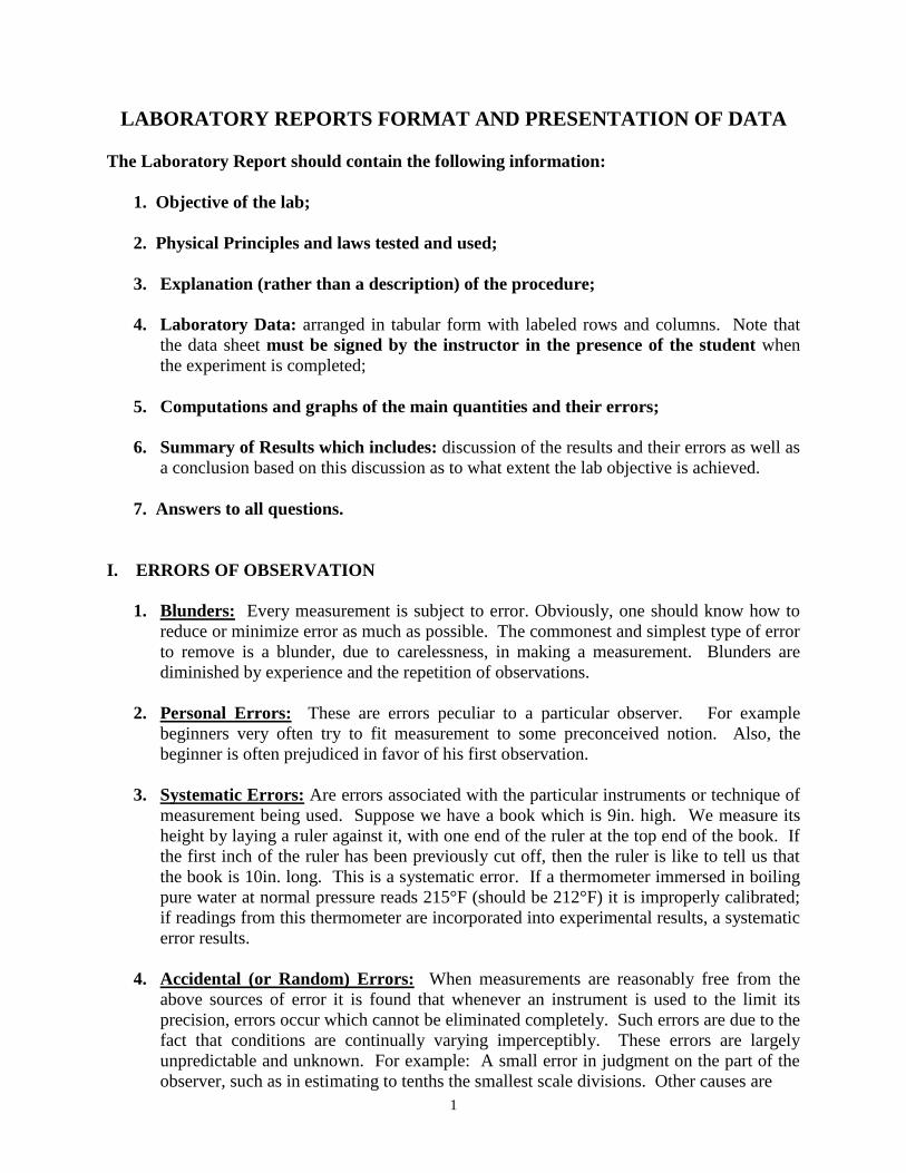
LABORATORY REPORTS FORMAT AND PRESENTATION OF DATA

The Laboratory Report should contain the following information:

1. Objective of the lab;

2. Physical Principles and laws tested and used;

3. Explanation (rather than a description) of the procedure;

4. Laboratory Data: arranged in tabular form with labeled rows and columns. Note that

the data sheet must be signed by the instructor in the presence of the student when

the experiment is completed;

5. Computations and graphs of the main quantities and their errors;

6. Summary of Results which includes: discussion of the results and their errors as well as

a conclusion based on this discussion as to what extent the lab objective is achieved.

7. Answers to all questions.

I. ERRORS OF OBSERVATION

1. Blunders: Every measurement is subject to error. Obviously, one should know how to

reduce or minimize error as much as possible. The commonest and simplest type of error

to remove is a blunder, due to carelessness, in making a measurement. Blunders are

diminished by experience and the repetition of observations.

2. Personal Errors: These are errors peculiar to a particular observer. For example

beginners very often try to fit measurement to some preconceived notion. Also, the

beginner is often prejudiced in favor of his first observation.

3. Systematic Errors: Are errors associated with the particular instruments or technique of

measurement being used. Suppose we have a book which is 9in. high. We measure its

height by laying a ruler against it, with one end of the ruler at the top end of the book. If

the first inch of the ruler has been previously cut off, then the ruler is like to tell us that

the book is 10in. long. This is a systematic error. If a thermometer immersed in boiling

pure water at normal pressure reads 215°F (should be 212°F) it is improperly calibrated;

if readings from this thermometer are incorporated into experimental results, a systematic

error results.

4. Accidental (or Random) Errors: When measurements are reasonably free from the

above sources of error it is found that whenever an instrument is used to the limit its

precision, errors occur which cannot be eliminated completely. Such errors are due to the

fact that conditions are continually varying imperceptibly. These errors are largely

unpredictable and unknown. For example: A small error in judgment on the part of the

observer, such as in estimating to tenths the smallest scale divisions. Other causes are

2

unpredictable fluctuations in conditions, such as temperature, illumination, socket voltage

or any kind of mechanical vibrations of the equipment being used. The effect of these

errors may be mitigated by repeating the measurement several times and taking the

average of the readings.

There are two ways of estimating the error due to random independent measurements.

One way is to calculate the Mean Absolute Deviation and the other is to calculate the

Standard deviation. Both methods are discussed in the appendix.

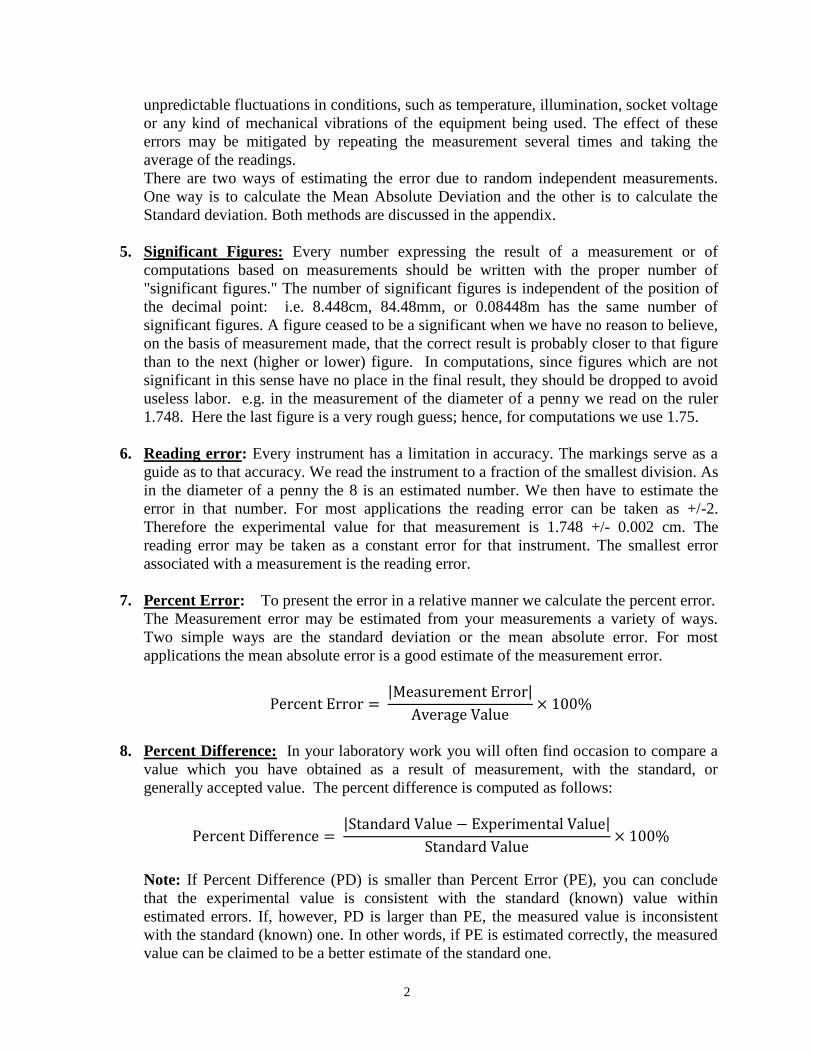
5. Significant Figures: Every number expressing the result of a measurement or of

computations based on measurements should be written with the proper number of

"significant figures." The number of significant figures is independent of the position of

the decimal point: i.e. 8.448cm, 84.48mm, or 0.08448m has the same number of

significant figures. A figure ceased to be a significant when we have no reason to believe,

on the basis of measurement made, that the correct result is probably closer to that figure

than to the next (higher or lower) figure. In computations, since figures which are not

significant in this sense have no place in the final result, they should be dropped to avoid

useless labor. e.g. in the measurement of the diameter of a penny we read on the ruler

1.748. Here the last figure is a very rough guess; hence, for computations we use 1.75.

6. Reading error: Every instrument has a limitation in accuracy. The markings serve as a

guide as to that accuracy. We read the instrument to a fraction of the smallest division. As

in the diameter of a penny the 8 is an estimated number. We then have to estimate the

error in that number. For most applications the reading error can be taken as +/-2.

Therefore the experimental value for that measurement is 1.748 +/- 0.002 cm. The

reading error may be taken as a constant error for that instrument. The smallest error

associated with a measurement is the reading error.

7. Percent Error: To present the error in a relative manner we calculate the percent error.

The Measurement error may be estimated from your measurements a variety of ways.

Two simple ways are the standard deviation or the mean absolute error. For most

applications the mean absolute error is a good estimate of the measurement error.

Percent Error = |Measurement Error|

Average Value× 100%

8. Percent Difference: In your laboratory work you will often find occasion to compare a

value which you have obtained as a result of measurement, with the standard, or

generally accepted value. The percent difference is computed as follows:

Percent Difference = |Standard Value − Experimental Value|

Standard Value× 100%

Note: If Percent Difference (PD) is smaller than Percent Error (PE), you can conclude

that the experimental value is consistent with the standard (known) value within

estimated errors. If, however, PD is larger than PE, the measured value is inconsistent

with the standard (known) one. In other words, if PE is estimated correctly, the measured

value can be claimed to be a better estimate of the standard one.

3

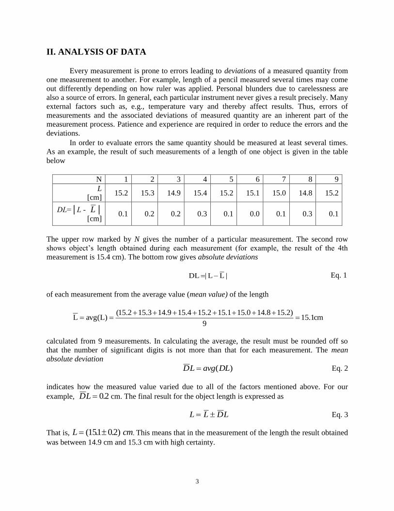
II. ANALYSIS OF DATA

Every measurement is prone to errors leading to deviations of a measured quantity from

one measurement to another. For example, length of a pencil measured several times may come

out differently depending on how ruler was applied. Personal blunders due to carelessness are

also a source of errors. In general, each particular instrument never gives a result precisely. Many

external factors such as, e.g., temperature vary and thereby affect results. Thus, errors of

measurements and the associated deviations of measured quantity are an inherent part of the

measurement process. Patience and experience are required in order to reduce the errors and the

deviations.

In order to evaluate errors the same quantity should be measured at least several times.

As an example, the result of such measurements of a length of one object is given in the table

below

N 1 2 3 4 5 6 7 8 9

L

[cm] 15.2 15.3 14.9 15.4 15.2 15.1 15.0 14.8 15.2

DL=L - L

[cm] 0.1 0.2 0.2 0.3 0.1 0.0 0.1 0.3 0.1

The upper row marked by N gives the number of a particular measurement. The second row

shows object’s length obtained during each measurement (for example, the result of the 4th

measurement is 15.4 cm). The bottom row gives absolute deviations

|LL|DL Eq. 1

of each measurement from the average value (mean value) of the length

cm1.159

)2.158.140.151.152.154.159.143.152.15()L(avgL

calculated from 9 measurements. In calculating the average, the result must be rounded off so

that the number of significant digits is not more than that for each measurement. The mean

absolute deviation

DL avg DL ( ) Eq. 2

indicates how the measured value varied due to all of the factors mentioned above. For our

example, DL 02. cm. The final result for the object length is expressed as

L L DL Eq. 3

That is, L cm ( . . )151 02 . This means that in the measurement of the length the result obtained

was between 14.9 cm and 15.3 cm with high certainty.

4

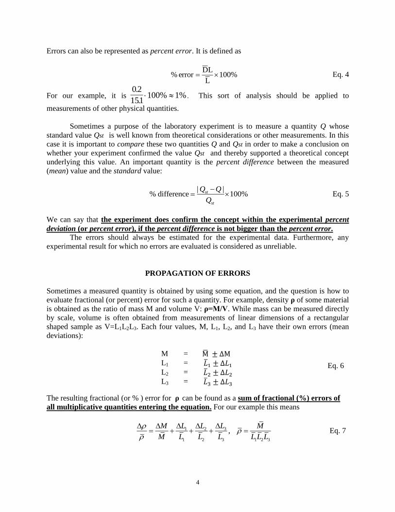
Errors can also be represented as percent error. It is defined as

%100L

LD error % Eq. 4

For our example, it is 0 2

151100% 1%

.

. . This sort of analysis should be applied to

measurements of other physical quantities.

Sometimes a purpose of the laboratory experiment is to measure a quantity Q whose

standard value Qst is well known from theoretical considerations or other measurements. In this

case it is important to compare these two quantities Q and Qst in order to make a conclusion on

whether your experiment confirmed the value Qst and thereby supported a theoretical concept

underlying this value. An important quantity is the percent difference between the measured

(mean) value and the standard value:

| |

% difference 100%st

st

Q Q

Q

Eq. 5

We can say that the experiment does confirm the concept within the experimental percent

deviation (or percent error), if the percent difference is not bigger than the percent error.

The errors should always be estimated for the experimental data. Furthermore, any

experimental result for which no errors are evaluated is considered as unreliable.

PROPAGATION OF ERRORS

Sometimes a measured quantity is obtained by using some equation, and the question is how to

evaluate fractional (or percent) error for such a quantity. For example, density ρ of some material

is obtained as the ratio of mass M and volume V: ρ=M/V. While mass can be measured directly

by scale, volume is often obtained from measurements of linear dimensions of a rectangular

shaped sample as V=L1L2L3. Each four values, M, L1, L2, and L3 have their own errors (mean

deviations):

The resulting fractional (or % ) error for ρ can be found as a sum of fractional (%) errors of

all multiplicative quantities entering the equation. For our example this means

31 2

1 2 3 1 2 3

, LL LM M

M L L L L L L

Eq. 7

M = M ± ∆M L1 = 1 ± ∆𝐿1 L2 = 2 ± ∆𝐿2 L3 = 3 ± ∆𝐿3

Eq. 6

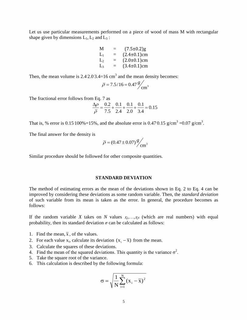
5

Let us use particular measurements performed on a piece of wood of mass M with rectangular

shape given by dimensions L1, L2 and L3 :

Then, the mean volume is 2.4.2.0

.3.4=16 cm

3 and the mean density becomes:

3 7.5 /16 0.47cm

g

The fractional error follows from Eq. 7 as

0.2 0.1 0.1 0.1 0.15

7.5 2.4 2.0 3.4

That is, % error is 0.15.100%=15%, and the absolute error is 0.47

.0.15 g/cm

3 =0.07 g/cm

3.

The final answer for the density is

3 (0.47 0.07)cm

g

Similar procedure should be followed for other composite quantities.

STANDARD DEVIATION

The method of estimating errors as the mean of the deviations shown in Eq. 2 to Eq. 4 can be

improved by considering these deviations as some random variable. Then, the standard deviation

of such variable from its mean is taken as the error. In general, the procedure becomes as

follows:

If the random variable X takes on N values x1,…,xN (which are real numbers) with equal

probability, then its standard deviation σ can be calculated as follows:

1. Find the mean, x , of the values.

2. For each value xi, calculate its deviation )xx( i from the mean.

3. Calculate the squares of these deviations.

4. Find the mean of the squared deviations. This quantity is the variance σ2.

5. Take the square root of the variance.

6. This calculation is described by the following formula:

M = (7.5±0.2)g L1 = (2.4±0.1)cm L2 = (2.0±0.1)cm L3 = (3.4±0.1)cm

N

1i

2

i )xx(N

1

6

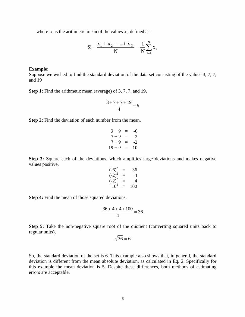
where x is the arithmetic mean of the values xi, defined as:

Example:

Suppose we wished to find the standard deviation of the data set consisting of the values 3, 7, 7,

and 19

Step 1: Find the arithmetic mean (average) of 3, 7, 7, and 19,

94

19773

Step 2: Find the deviation of each number from the mean,

3 − 9 = -6

7 − 9 = -2

7 − 9 = -2

19 − 9 = 10

Step 3: Square each of the deviations, which amplifies large deviations and makes negative

values positive,

(-6)2 = 36

(-2)2 = 4

(-2)2 = 4

102 = 100

Step 4: Find the mean of those squared deviations,

Step 5: Take the non-negative square root of the quotient (converting squared units back to

regular units),

So, the standard deviation of the set is 6. This example also shows that, in general, the standard

deviation is different from the mean absolute deviation, as calculated in Eq. 2. Specifically for

this example the mean deviation is 5. Despite these differences, both methods of estimating

errors are acceptable.

N

1i

iN21 x

N

1

N

x...xxx

364

1004436

636

7

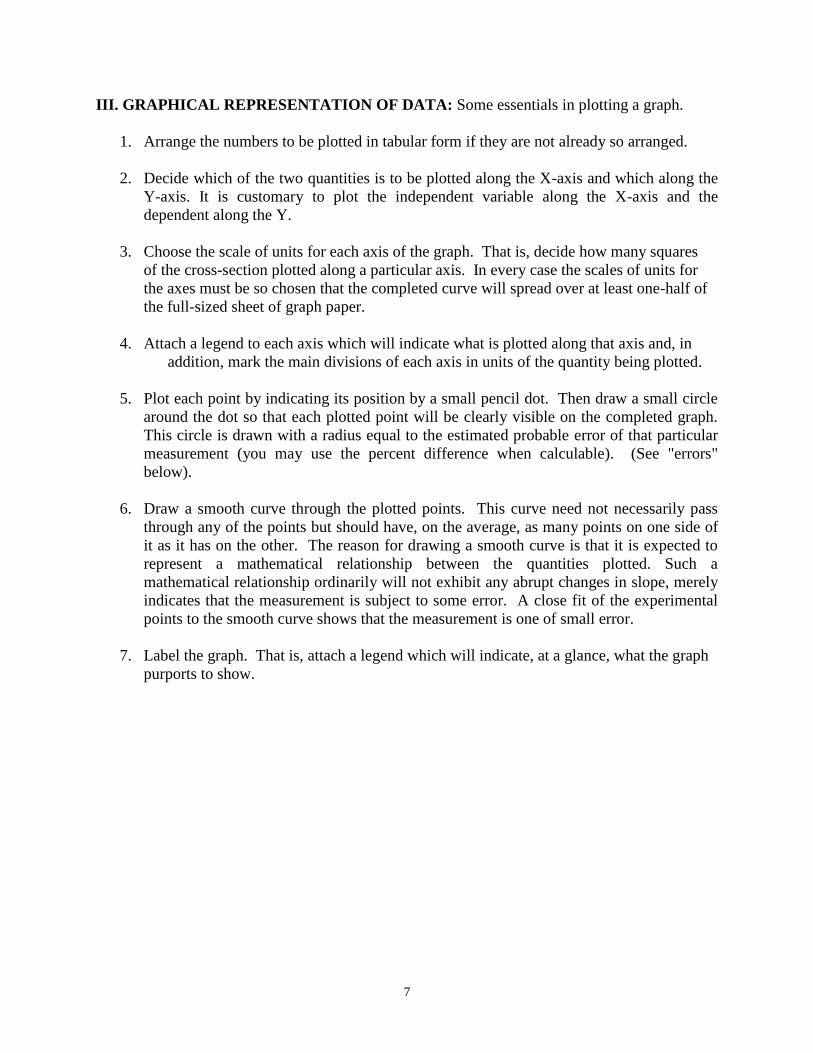
III. GRAPHICAL REPRESENTATION OF DATA: Some essentials in plotting a graph.

1. Arrange the numbers to be plotted in tabular form if they are not already so arranged.

2. Decide which of the two quantities is to be plotted along the X-axis and which along the

Y-axis. It is customary to plot the independent variable along the X-axis and the

dependent along the Y.

3. Choose the scale of units for each axis of the graph. That is, decide how many squares

of the cross-section plotted along a particular axis. In every case the scales of units for

the axes must be so chosen that the completed curve will spread over at least one-half of

the full-sized sheet of graph paper.

4. Attach a legend to each axis which will indicate what is plotted along that axis and, in

addition, mark the main divisions of each axis in units of the quantity being plotted.

5. Plot each point by indicating its position by a small pencil dot. Then draw a small circle

around the dot so that each plotted point will be clearly visible on the completed graph.

This circle is drawn with a radius equal to the estimated probable error of that particular

measurement (you may use the percent difference when calculable). (See "errors"

below).

6. Draw a smooth curve through the plotted points. This curve need not necessarily pass

through any of the points but should have, on the average, as many points on one side of

it as it has on the other. The reason for drawing a smooth curve is that it is expected to

represent a mathematical relationship between the quantities plotted. Such a

mathematical relationship ordinarily will not exhibit any abrupt changes in slope, merely

indicates that the measurement is subject to some error. A close fit of the experimental

points to the smooth curve shows that the measurement is one of small error.

7. Label the graph. That is, attach a legend which will indicate, at a glance, what the graph

purports to show.

8

MASS AND DENSITY

Apparatus:

- Electronic balance- Vernier caliper or metric ruler- Assorted metallic cylinders- Aluminum bar- Wooden block- Irregular shaped object (mineral/rock sample)- 250ml graduated cylinder

Part I. Mass and Weight:

The mass of a body at rest is an invariable property of that body. It is a measure of the quantityof matter in a body. A body has the same mass at the equator as at the North Pole, -- the same masson the earth as on Jupiter or interstellar space.

The gravitational force between the earth (or other planet) and a body is called the weight of thebody with respect to the earth (or other planet). The gravitational force on a body is a variablequantity even on the surface of the earth, e.g., the weight of a body is larger at the North Pole thanat the Equator. E.g., A book transported to the moon would have the same mass (quantity matter)on the moon as it had back on the earth, but the book weighs less on the moon than it did on the earthbecause the moon's gravitational pull is less than the earth's.

The weight of a body is proportional to its mass, the proportionality factor depending on theplace at which the weight is determined. If the weight of a body is compared with that of a standardbody, at the same place on the earth the ratio of the two weights is equal to the ratio of the twomasses. Consequently, if the weight of the body is found to be equal to the weight of a standardbody at the same place on earth, the two masses are equal. In order to measure the mass of a body,it is necessary to find a standard mass or a combination of standard masses whose weight equals thatof a body at the same place on the earth. The device employed for this purpose is called a balance.

Part I - Obtaining the mass:

1.1. Determine the mass of each object using the balance. Record all data in tabular form.

Part II - Volume based on measured dimensions:

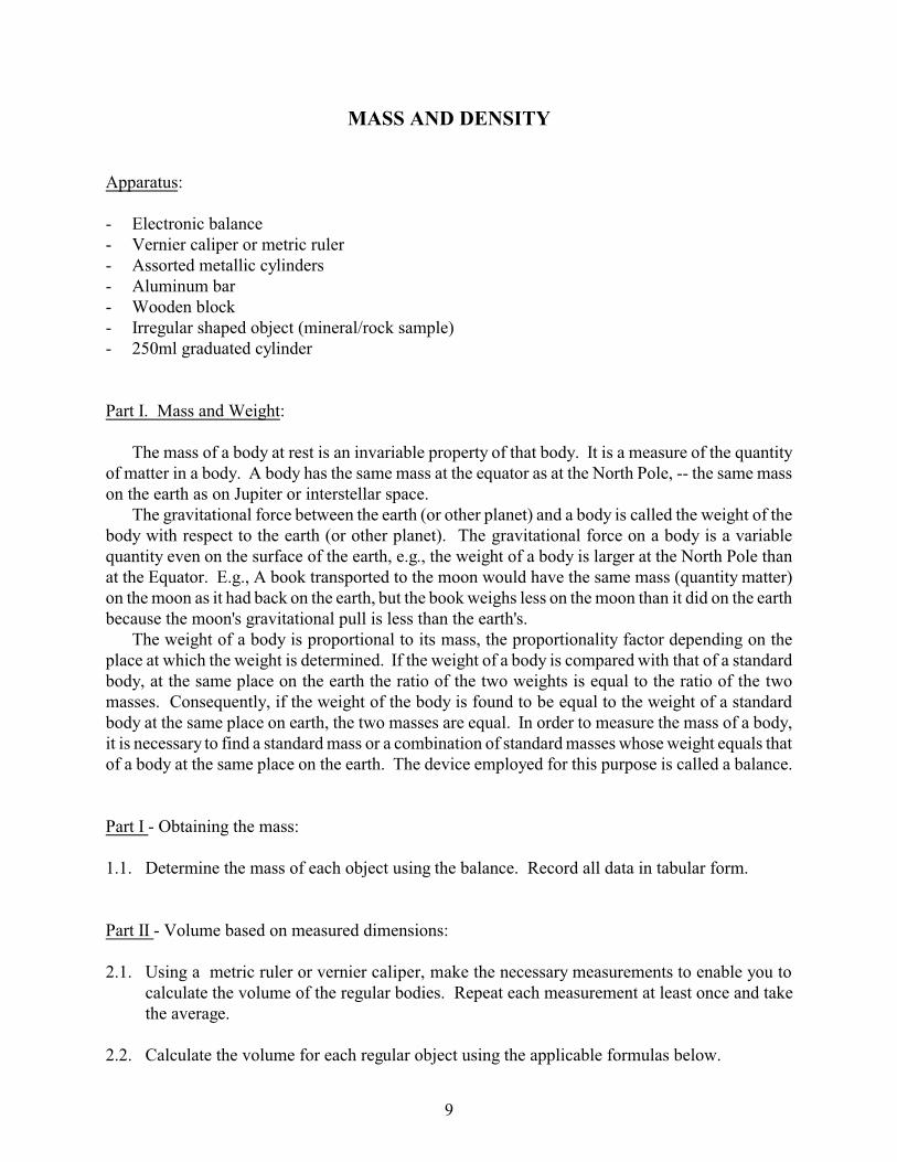
2.1. Using a metric ruler or vernier caliper, make the necessary measurements to enable you tocalculate the volume of the regular bodies. Repeat each measurement at least once and takethe average.

2.2. Calculate the volume for each regular object using the applicable formulas below.

9

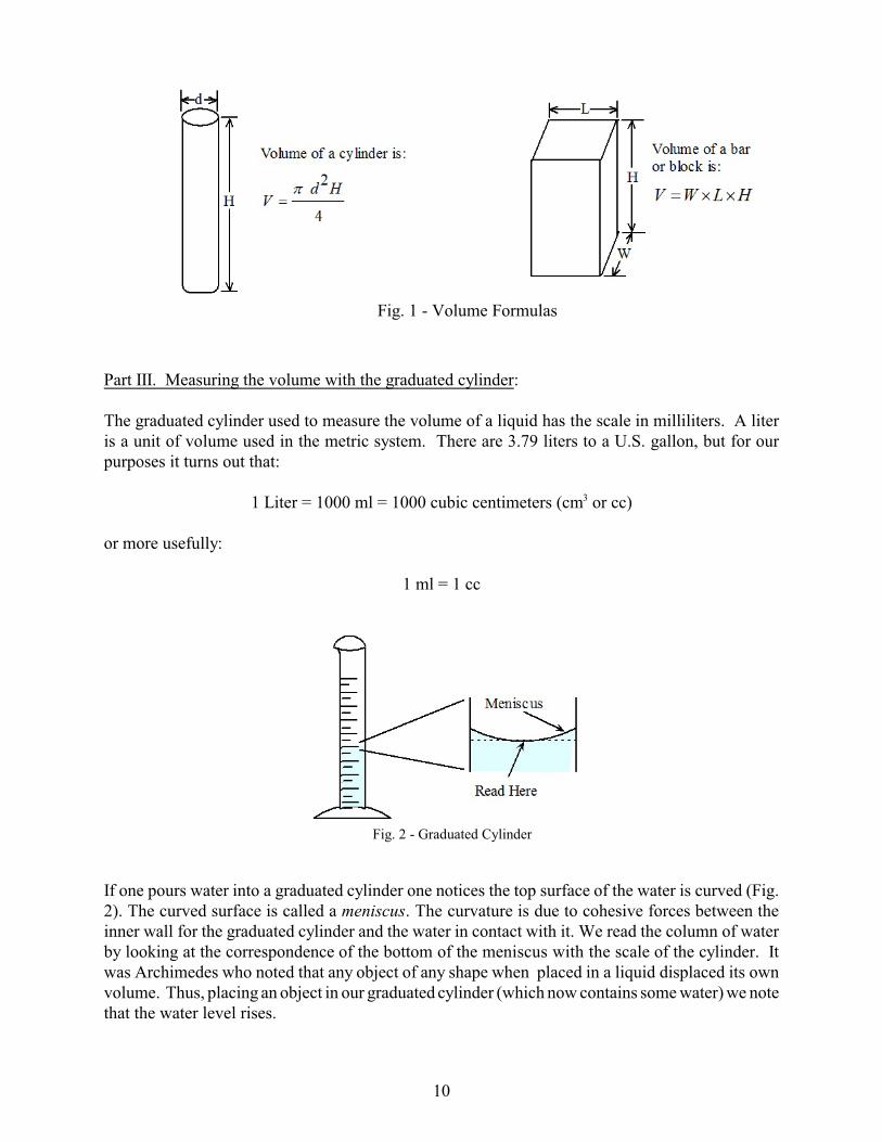
Fig. 2 - Graduated Cylinder

Part III. Measuring the volume with the graduated cylinder:

The graduated cylinder used to measure the volume of a liquid has the scale in milliliters. A literis a unit of volume used in the metric system. There are 3.79 liters to a U.S. gallon, but for ourpurposes it turns out that:

1 Liter = 1000 ml = 1000 cubic centimeters (cm3 or cc)

or more usefully:

1 ml = 1 cc

If one pours water into a graduated cylinder one notices the top surface of the water is curved (Fig.2). The curved surface is called a meniscus. The curvature is due to cohesive forces between theinner wall for the graduated cylinder and the water in contact with it. We read the column of waterby looking at the correspondence of the bottom of the meniscus with the scale of the cylinder. It was Archimedes who noted that any object of any shape when placed in a liquid displaced its ownvolume. Thus, placing an object in our graduated cylinder (which now contains some water) we notethat the water level rises.

Fig. 1 - Volume Formulas

10

3.1 Use the graduated cylinder to obtain the volume of the objects applicable to this method. Beingenious with the wooden block!

Part IV. Mass Density:

The “mass density” of a material is defined as the mass of any amount of that material divided bythe volume of that amount. The density of a substance is a fixed quantity for fixed externalconditions, and, thus, is a means of identifying a substance. E.g., All different shaped solids ofaluminum have the same density at room temperature. The units of mass density are g/cm3 or kg/m3

in the metric system.

When we use centimeter (cm), grams (g), and seconds (s) in measuring quantities we refer to the cgssystem. Likewise when we use meters (m), kilograms (kg), and seconds (s) we refer to the mkssystem.

4.1. Calculate the mass density of each object in the cgs system.

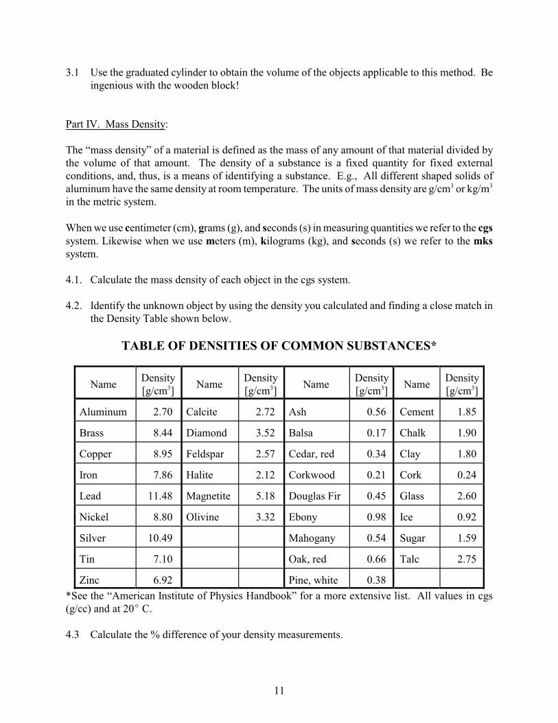
4.2. Identify the unknown object by using the density you calculated and finding a close match inthe Density Table shown below.

TABLE OF DENSITIES OF COMMON SUBSTANCES*

Name Density[g/cm3]

NameDensity[g/cm3]

NameDensity[g/cm3]

NameDensity[g/cm3]

Aluminum 2.70 Calcite 2.72 Ash 0.56 Cement 1.85

Brass 8.44 Diamond 3.52 Balsa 0.17 Chalk 1.90

Copper 8.95 Feldspar 2.57 Cedar, red 0.34 Clay 1.80

Iron 7.86 Halite 2.12 Corkwood 0.21 Cork 0.24

Lead 11.48 Magnetite 5.18 Douglas Fir 0.45 Glass 2.60

Nickel 8.80 Olivine 3.32 Ebony 0.98 Ice 0.92

Silver 10.49 Mahogany 0.54 Sugar 1.59

Tin 7.10 Oak, red 0.66 Talc 2.75

Zinc 6.92 Pine, white 0.38

*See the “American Institute of Physics Handbook” for a more extensive list. All values in cgs(g/cc) and at 20E C.

4.3 Calculate the % difference of your density measurements.

11

Questions:

1. By Archimedes' observation how would you obtain the volume of the object placed in thecylinder?

2. Which value of the volume is closer to the 'truth'? I.e., Part II or III. Explain your answer.

3. How do you account for the errors in your computed values of the density(ies)?

4. Which type of measurement done in parts I, II and III do you think you made with the leasterror? i.e., mass or length or volume. Explain.

5. Which of the densities you have just determined would you expect to be the least accurate?

6. What is the benefit, if any, in measuring volumes by using Archimedes’ observations?

12

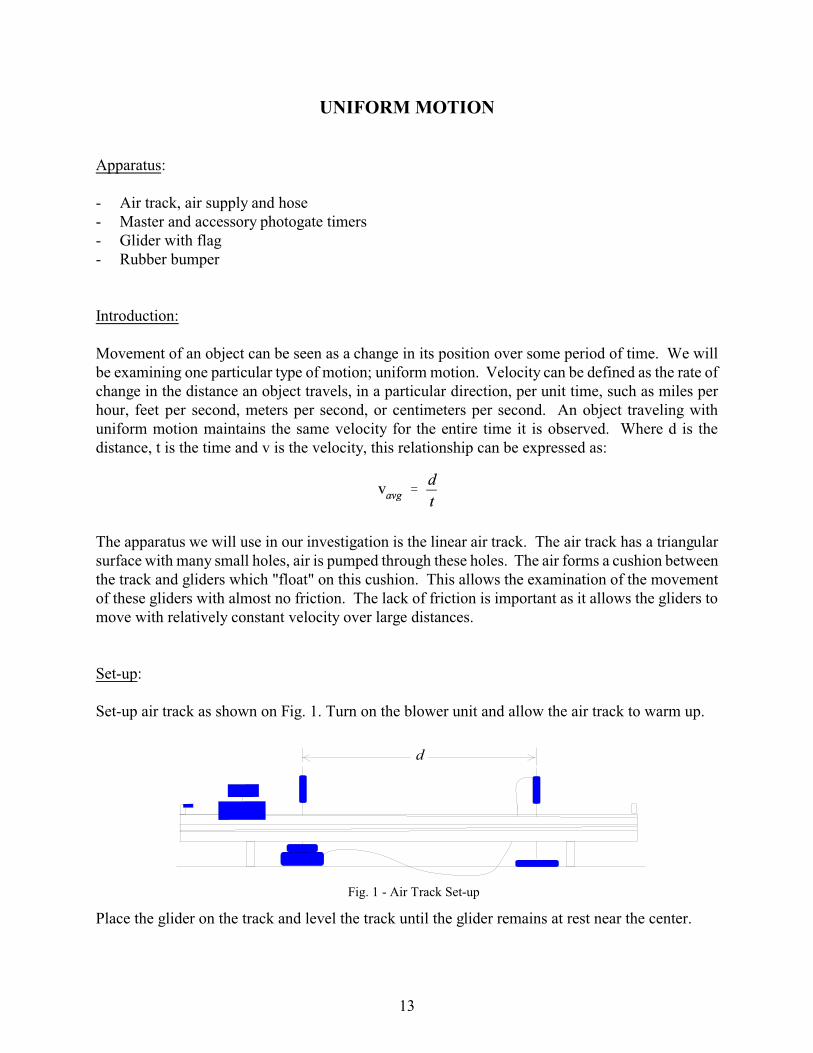
Fig. 1 - Air Track Set-up

UNIFORM MOTION

Apparatus:

- Air track, air supply and hose- Master and accessory photogate timers- Glider with flag- Rubber bumper

Introduction:

Movement of an object can be seen as a change in its position over some period of time. We willbe examining one particular type of motion; uniform motion. Velocity can be defined as the rate ofchange in the distance an object travels, in a particular direction, per unit time, such as miles perhour, feet per second, meters per second, or centimeters per second. An object traveling withuniform motion maintains the same velocity for the entire time it is observed. Where d is thedistance, t is the time and v is the velocity, this relationship can be expressed as:

The apparatus we will use in our investigation is the linear air track. The air track has a triangularsurface with many small holes, air is pumped through these holes. The air forms a cushion betweenthe track and gliders which "float" on this cushion. This allows the examination of the movementof these gliders with almost no friction. The lack of friction is important as it allows the gliders tomove with relatively constant velocity over large distances.

Set-up:

Set-up air track as shown on Fig. 1. Turn on the blower unit and allow the air track to warm up.

Place the glider on the track and level the track until the glider remains at rest near the center.

13

Procedure:

Position the start and stop photogates so that the distance between them is 20cm. Set the masterphotogate to pulse mode. With the rubber band set for the smallest separation, launch the glider andrecord the time. Be sure not to allow the glider to bounce back and trip the start gate before the timeis recorded. Repeat two more times for the same distance. Repeat the procedure after moving thestop photogate to give timing distances of 40cm, 60cm, 80cm and 100cm. Reset the timer each timebefore releasing the glider. Do not forget to do three runs for each distance and record thecorresponding times.

Data Table

d[cm]

t[s]

tavg

[s]v=d/tavg

[cm/s]

20

t1=

t2=

t3=

40

t1=

t2=

t3=

60

t1=

t2=

t3=

80

t1=

t2=

t3=

100

t1=

t2=

t3=

Calculations and Graph:

1. Calculate the average time for each given distance.

2. Use the average time to calculate the average velocity for each position. Compare thesevelocities are they equal? How much do you trust your results?

14

3. Use all the velocities on the 4th column and find the mean.

4. Use the data from the table to plot a graph of d vs. tavg.

5. Determine the slope of the graph, how does it compare to the mean velocity you obtained onCalculation 3?

15

16

MOTION OF A BODY IN FREE FALL

Apparatus:

- Behr Free-Fall apparatus- Pre-made tape from the free fall apparatus- Masking Tape- Ruler and/or meter stick

Discussion:

In the case of free falling objects the acceleration and the velocity are in the same direction so thatin this experiment we will be able to measure the acceleration by concerning ourselves only withchanges in the speed of the falling bodies. (We recall the definition of acceleration as a change inthe velocity per unit-time and the definition of velocity as the displacement in a specified directionper unit-time.)

A body is said to be in free fall when the only force that acts upon it is gravity. The condition of freefall is difficult to achieve in the laboratory because of the retarding frictional force produced by airresistance; to be more accurate we should perform the experiment in a vacuum. Since, however, theforce exerted by air resistance on a dense, compact object is small compared to the force of gravity,we will neglect it in this experiment.

The force exerted by gravity may be considered to be constant as long as we stay near the surfaceof the earth; i.e., the force acting on a body is independent of the position of the body. The force ofgravity (also known as the weight of the body) is given by the equation:

where m is the mass and g is the acceleration due to gravity

The direction of g is toward the center of the Earth. As shown by Galileo, the acceleration impartedto a body by gravity is independent of the mass of the body so that all bodies fall equally fast (in avacuum). The acceleration is also independent of the shape of the body (again neglecting airresistance).

Useful Information for Constant Acceleration:

17

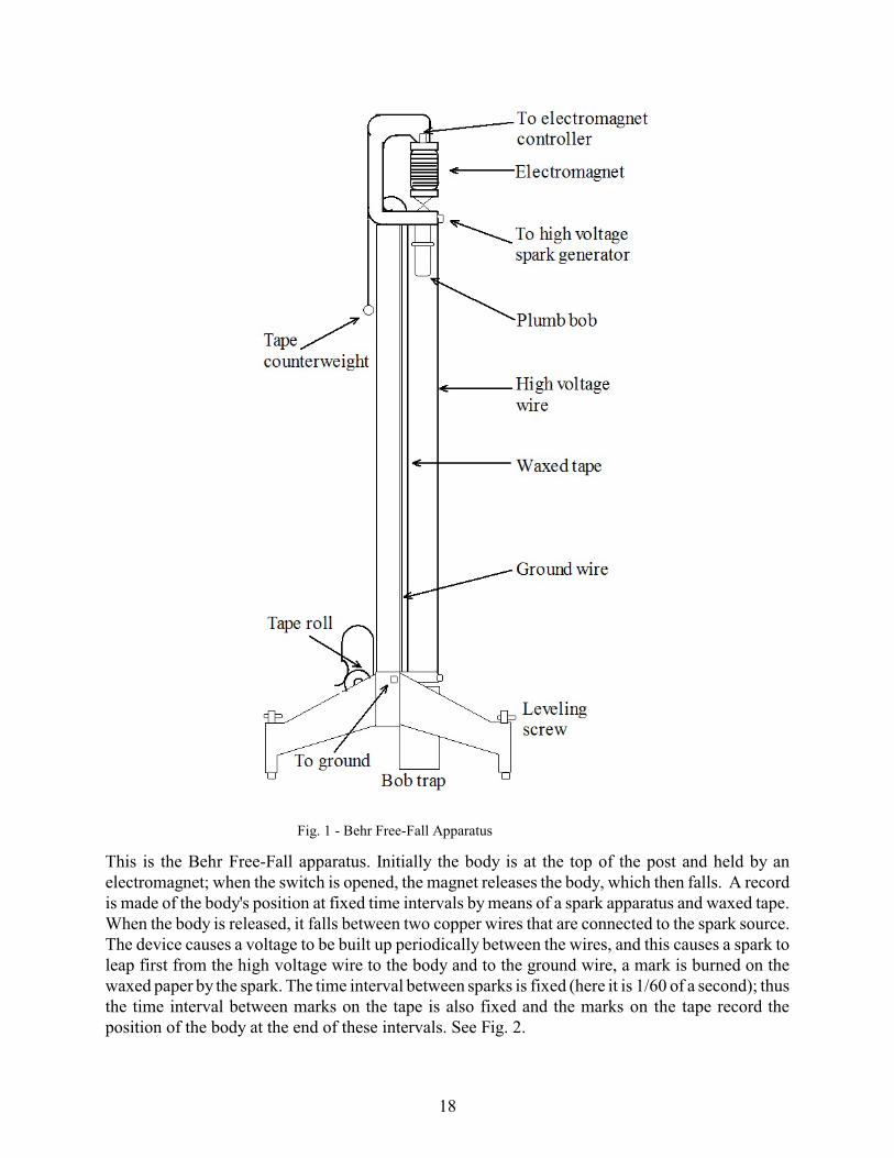
Fig. 1 - Behr Free-Fall Apparatus

This is the Behr Free-Fall apparatus. Initially the body is at the top of the post and held by anelectromagnet; when the switch is opened, the magnet releases the body, which then falls. A recordis made of the body's position at fixed time intervals by means of a spark apparatus and waxed tape. When the body is released, it falls between two copper wires that are connected to the spark source.The device causes a voltage to be built up periodically between the wires, and this causes a spark toleap first from the high voltage wire to the body and to the ground wire, a mark is burned on thewaxed paper by the spark. The time interval between sparks is fixed (here it is 1/60 of a second); thusthe time interval between marks on the tape is also fixed and the marks on the tape record theposition of the body at the end of these intervals. See Fig. 2.

18

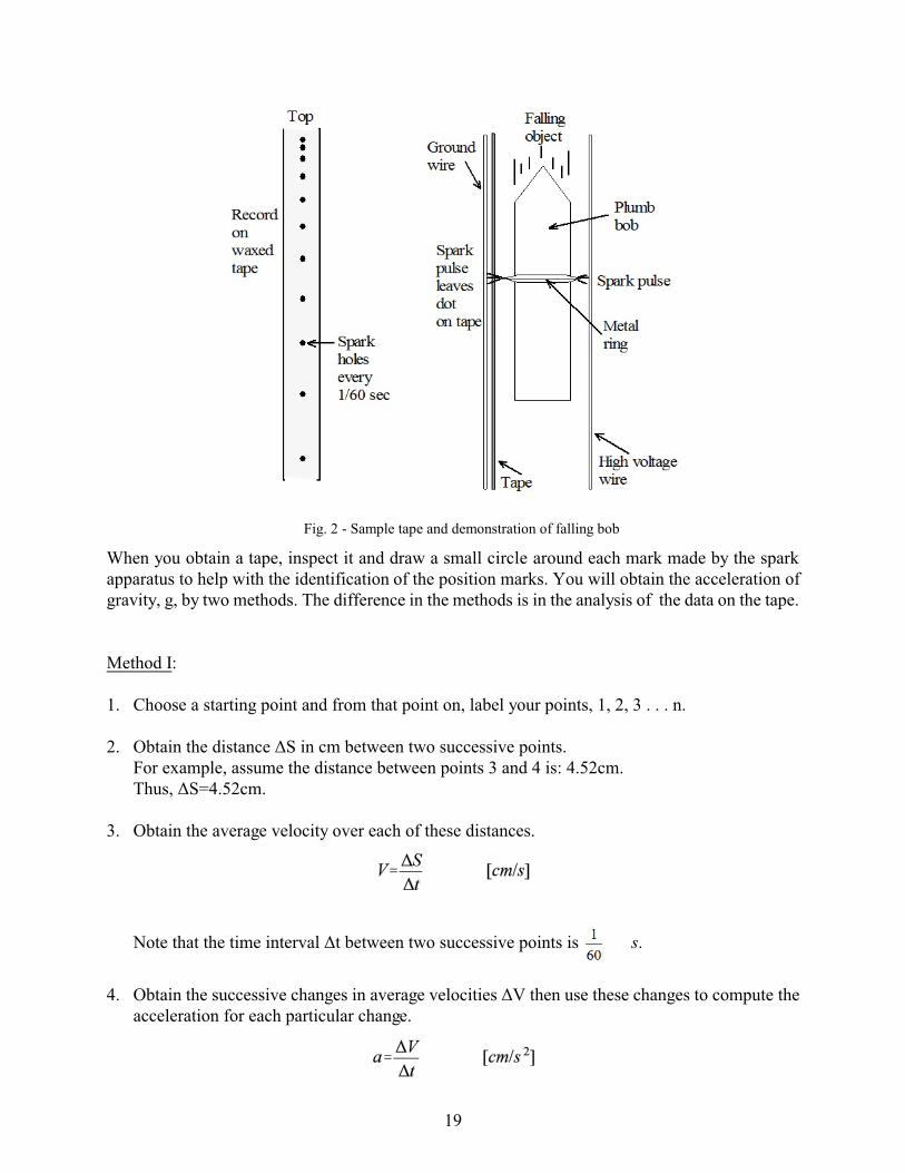
Fig. 2 - Sample tape and demonstration of falling bob

When you obtain a tape, inspect it and draw a small circle around each mark made by the sparkapparatus to help with the identification of the position marks. You will obtain the acceleration ofgravity, g, by two methods. The difference in the methods is in the analysis of the data on the tape.

Method I:

1. Choose a starting point and from that point on, label your points, 1, 2, 3 . . . n.

2. Obtain the distance ÄS in cm between two successive points. For example, assume the distance between points 3 and 4 is: 4.52cm. Thus, ÄS=4.52cm.

3. Obtain the average velocity over each of these distances.

Note that the time interval Ät between two successive points is s.

4. Obtain the successive changes in average velocities ÄV then use these changes to compute theacceleration for each particular change.

19

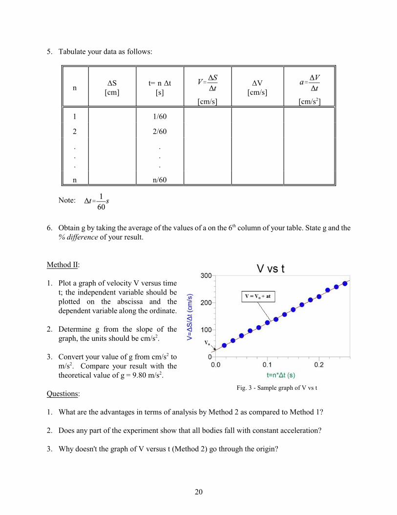
Fig. 3 - Sample graph of V vs t

5. Tabulate your data as follows:

nÄS

[cm]t= n Ät

[s] [cm/s]

ÄV[cm/s]

[cm/s2]

1 1/60

2 2/60

.

.

.

.

.

.

n n/60

Note:

6. Obtain g by taking the average of the values of a on the 6th column of your table. State g and the% difference of your result.

Method II:

1. Plot a graph of velocity V versus timet; the independent variable should beplotted on the abscissa and thedependent variable along the ordinate.

2. Determine g from the slope of thegraph, the units should be cm/s2.

3. Convert your value of g from cm/s2 tom/s2. Compare your result with thetheoretical value of g = 9.80 m/s2.

Questions:

1. What are the advantages in terms of analysis by Method 2 as compared to Method 1?

2. Does any part of the experiment show that all bodies fall with constant acceleration?

3. Why doesn't the graph of V versus t (Method 2) go through the origin?

20

FORCE AND ACCELERATION

Apparatus:

S Air track, air supply and hoseS Master and accessory photogate timersS Glider and Air track kitS Electronic balance

Introduction:

The interaction between various objects is responsible for a whole variety of phenomena in ourPhysical World. If no interaction existed our world would be a bunch of objects performing UniformMotion in accordance to Newton’s 1st Law. We could not even perceive such a world because outperceptions are associated with out interaction with the external environment. For example, visionis due to interaction with light. In fact, we would not even exist because no forces would bind theconstituents of our organisms together. What a boring situation!

So force is one of the central physical concepts. It is not possible for us to trace out all the possiblemeans by which various forces act, and what are all the implications. However, we will consider aspecific situation which can be studied completely. This is based on the observation that a forceapplied to a single object produces acceleration of this object. Furthermore, a constant forceproduces a constant acceleration. In accordance with Newton’s 2nd law of dynamics, the accelerationis proportional to the force. This law can be formulated as the concise equation:

F = MA Eq. 1

where A is the acceleration and F is the force. While F is essentially due to other objects, thecoefficient M is a property of the accelerating object. This property is called mass. Applying this

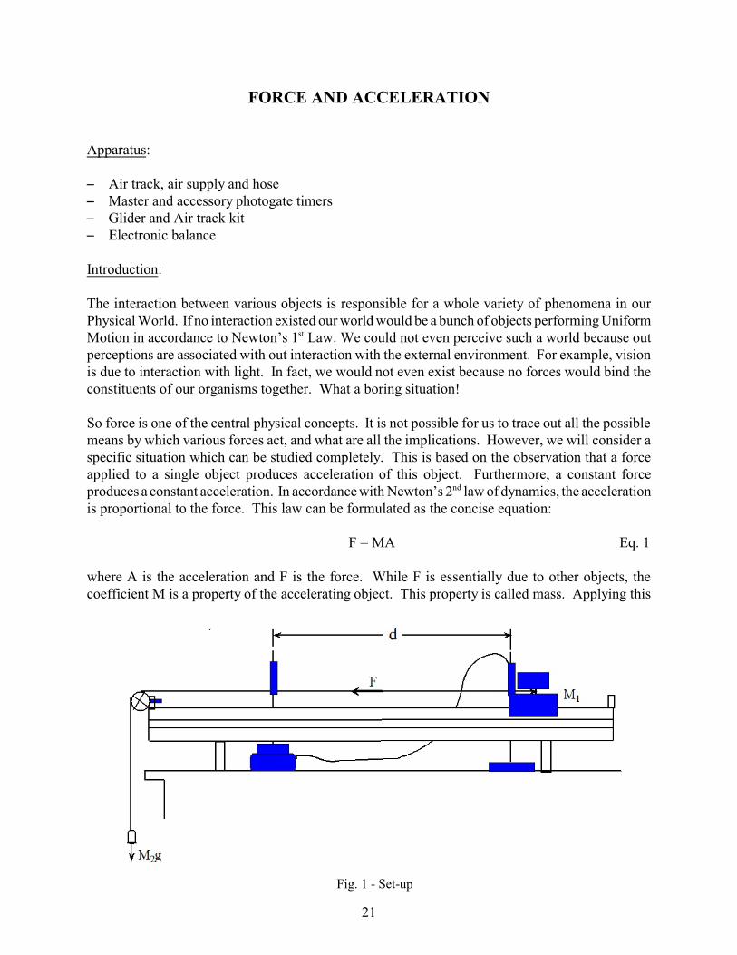
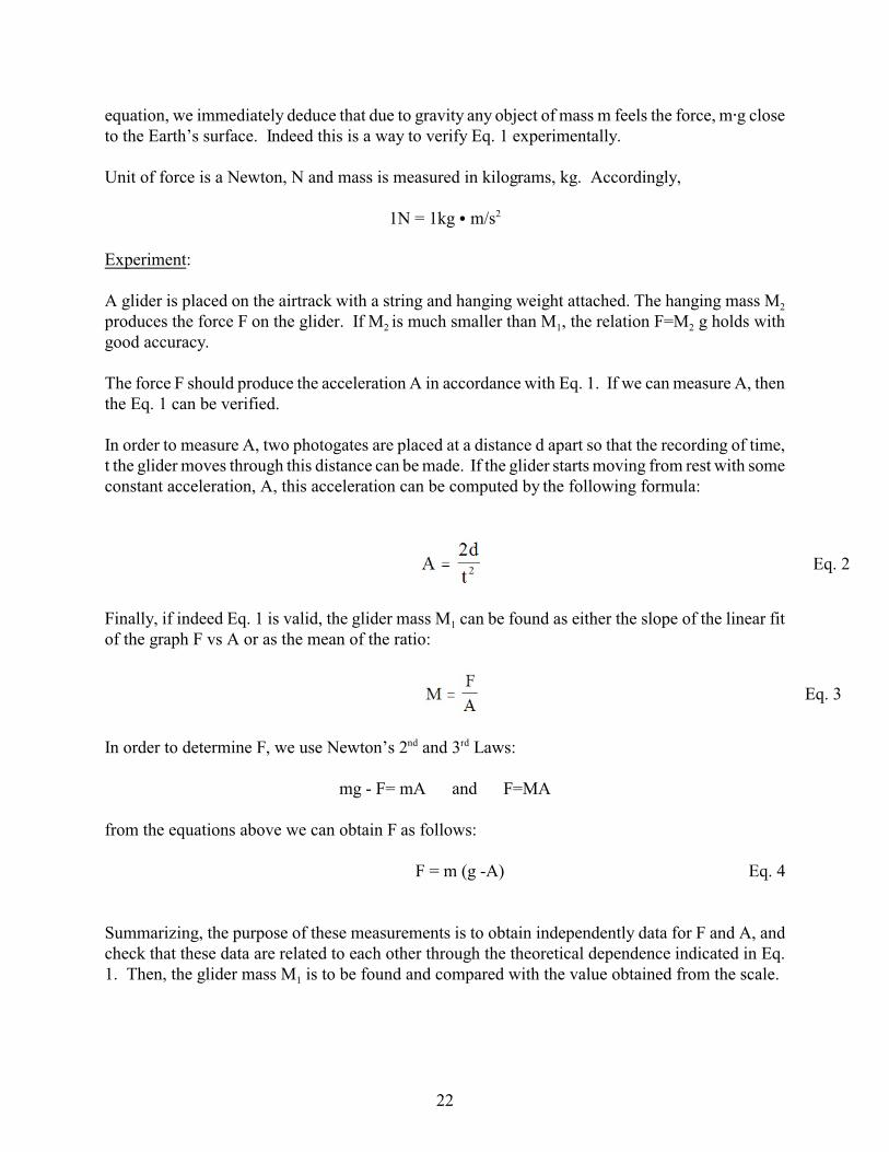
Fig. 1 - Set-up

21

equation, we immediately deduce that due to gravity any object of mass m feels the force, m@g closeto the Earth’s surface. Indeed this is a way to verify Eq. 1 experimentally.

Unit of force is a Newton, N and mass is measured in kilograms, kg. Accordingly,

1N = 1kg C m/s2

Experiment:

A glider is placed on the airtrack with a string and hanging weight attached. The hanging mass M2

produces the force F on the glider. If M2 is much smaller than M1, the relation F=M2 g holds withgood accuracy.

The force F should produce the acceleration A in accordance with Eq. 1. If we can measure A, thenthe Eq. 1 can be verified.

In order to measure A, two photogates are placed at a distance d apart so that the recording of time,t the glider moves through this distance can be made. If the glider starts moving from rest with someconstant acceleration, A, this acceleration can be computed by the following formula:

Eq. 2

Finally, if indeed Eq. 1 is valid, the glider mass M1 can be found as either the slope of the linear fitof the graph F vs A or as the mean of the ratio:

Eq. 3

In order to determine F, we use Newton’s 2nd and 3rd Laws:

mg - F= mA and F=MA

from the equations above we can obtain F as follows:

F = m (g -A) Eq. 4

Summarizing, the purpose of these measurements is to obtain independently data for F and A, andcheck that these data are related to each other through the theoretical dependence indicated in Eq.1. Then, the glider mass M1 is to be found and compared with the value obtained from the scale.

22

Preliminary set-up:

Turn on the air supply and allow the track to warm up for several minutes then level the air track. Cut a length of string approximately 130 cm long and tie a small loop at each end. Attach one endof the string to the glider by placing one loop around the connector for the flag, and the other end tothe mass hanger. Place the string over the pulley and set the position of the glider so that the massis just below the pulley. Place the photogates 60-80cm apart making sure that the hanger does nothit the floor before the glider crosses through the gate closer to the pulley. Adjust the position of thestart photogate so that it is about to be tripped by the glider. Set master photogate to pulse mode.

Procedure:

1. Weigh the glider, flag and string and record the total mass as M1 (units in kg). If you wish forthe glider to be heavier there is the option to add 50 g weights, one on each side of the glider.

2. The hanger by itself weighs 2 g (0.002 kg). Place 5 g (0.005 kg) on the hanger to get a total massM2= 7 g = 0.007 kg. When ready, release the glider and record the time. Repeat two additionaltimes.

3. Combine the small masses to give additional total hanging masses of 12,17, 22, and 27 grams. Take three time measurements for each and record them.

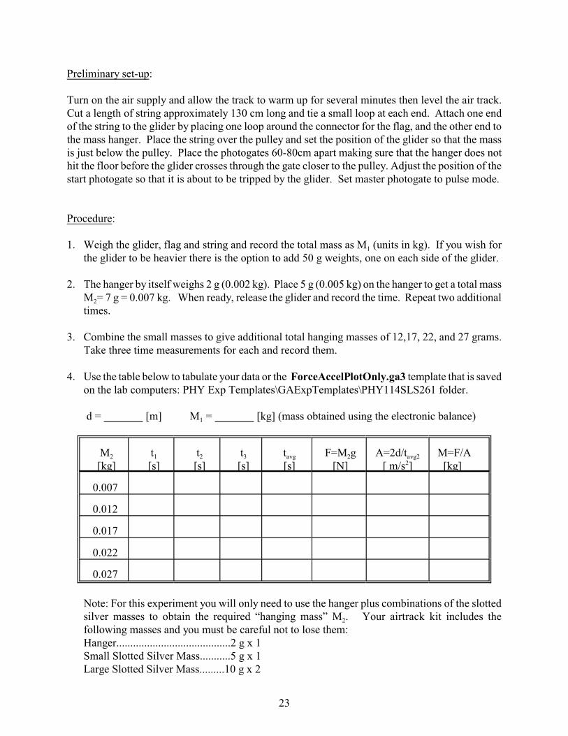
4. Use the table below to tabulate your data or the ForceAccelPlotOnly.ga3 template that is savedon the lab computers: PHY Exp Templates\GAExpTemplates\PHY114SLS261 folder.

d = [m] M1 = [kg] (mass obtained using the electronic balance)

M2

[kg] t1

[s] t2

[s] t3

[s] tavg

[s]F=M2g

[N]A=2d/tavg2

[ m/s2]M=F/A [kg]

0.007

0.012

0.017

0.022

0.027

Note: For this experiment you will only need to use the hanger plus combinations of the slottedsilver masses to obtain the required “hanging mass” M2. Your airtrack kit includes thefollowing masses and you must be careful not to lose them:Hanger.........................................2 g x 1Small Slotted Silver Mass...........5 g x 1Large Slotted Silver Mass.........10 g x 2

23

Graph/Calculations:

1. From the table of Procedure 5 plot a graph of F vs. A. Find the slope of the best linear fit forthis graph and record it. What should the slope of this graph represent? If you are using theGraphical Analysis template ForceAccelPlotOnly.ga3 click on f(x) on top of the toolbar andselect “proportional” fit to obtain the slope of the line.

2. Compare M1 (mass of the glider) to the other M values that were obtained based on experimentaldata.

Questions:

1. How close is the value of the glider mass obtained from the slope to the one obtained from theelectronic balance?

2. How close is the value of the glider mass obtained from the mean of the F/A ratio (last columnof your data table) to the one obtained from the electronic balance?

3. Give a conclusion as to whether this experiment supports Newton’s 2nd Law of dynamics. Discuss the precision of your measurements for the glider mass, and possible reasons fordeviations.

24

Eq. 1

Eq. 2

MECHANICAL WORK AND ENERGY

Apparatus:

S Air track, air supply and hoseS Master photogate timerS Glider and Air track kitS Electronic balance

Objective: The concept of Work and Energy is to be studied. The Law of Conservation of Energy is to beverified for a simple mechanical set-up.

Theoretical Background: The concept of Work and Energy is crucial for understanding nature. Its importance is not limitedto the mechanics of a single object. This concept can equally be applied to complex systems–atoms,molecules, substance, and even organisms. All acts of motion, transformation, and creation in ourworld are due to Work and Energy. We will begin study of this concept for a simple mechanicalsystem–the glider on the airtrack.A very special significance is endowed to the Law of Conservation of Energy which states that thetotal amount of Energy in the world is constant. That is, Energy can neither be created or destroyed.It can be only transformed from one form to another and redistributed between objects. The processof Energy transformation and redistribution is called Work.How Energy is defined and measured is to be studied in this experiment, though here we will talkonly about Mechanical Energy and Work. The first form of energy we will investigate is Kinetic Energy. This is energy or ability to do work,that an object possesses due to its motion. In this case if we know the mass of an object and itsvelocity, we can calculate its kinetic energy:

The larger the object mass, M or the velocity, V, the greater the KE. If two moving bodies areconsidered then their total kinetic energy is:

The second form of energy we will investigate is Potential Energy. This is the energy or ability todo work, that an object possesses due to its height or position. In our experiment we will only dealwith objects raised a certain height above either the ground or some reference point. If we know themass of an object and its height we can calculate its potential energy:

25

Eq. 3

Eq. 4

The unit of energy is the Joule, J where:

If the mechanical system is isolated from the environment, the total Mechanical Energy is:

In other words, the total mechanical energy is conserved, in accordance with the general statementgiven above.Mechanical energy can be lost or acquired, if it is transformed to or from other forms of energy. Foexample, friction decreased the KE and heats the environment. If, however, no friction is present,Eq. 3 says that any increase in KE occurs at the expense of PE, or conversely any increase of PEoccurs at the expense of KE. Reformulated in terms of the change of Kinetic Energy, ÄKE and thechange in Potential Energy, ÄPE, the statement becomes

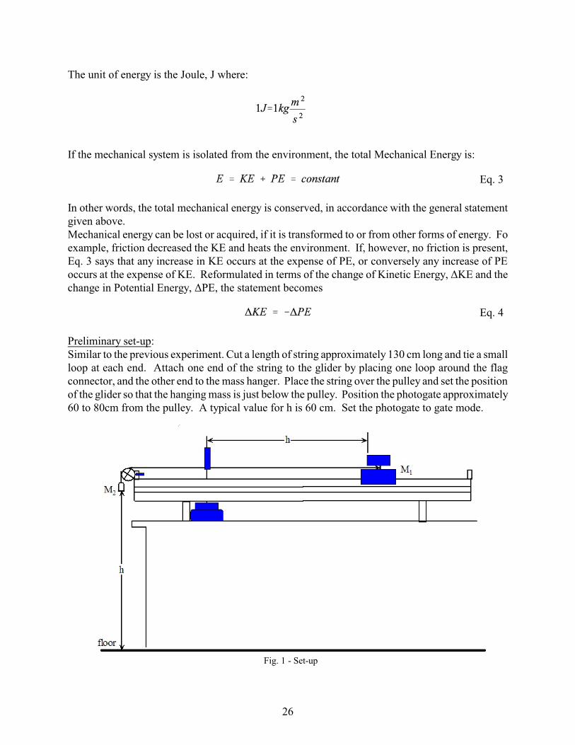
Preliminary set-up:Similar to the previous experiment. Cut a length of string approximately 130 cm long and tie a smallloop at each end. Attach one end of the string to the glider by placing one loop around the flagconnector, and the other end to the mass hanger. Place the string over the pulley and set the positionof the glider so that the hanging mass is just below the pulley. Position the photogate approximately60 to 80cm from the pulley. A typical value for h is 60 cm. Set the photogate to gate mode.

Fig. 1 - Set-up

26

Procedure:

1. Weigh the glider with the flag and string and record the total mass as M1 with units in kg. If youwish for the glider to be heavier there is the option to add 50 g weights, one on each side of theglider.

2. The hanger by itself weighs 2 g (0.002 kg). Place 5 g (0.005 kg) on the hanger to get a total mass

M2 = 7 g = 0.007 kg as shown on the table below. When ready release the glider M1. Recordthe time. Repeat two additional times.

3. Combine the small masses to give additional total hanging masses of 12,17, 22, and 27 grams. Take three time measurements for each and record them.

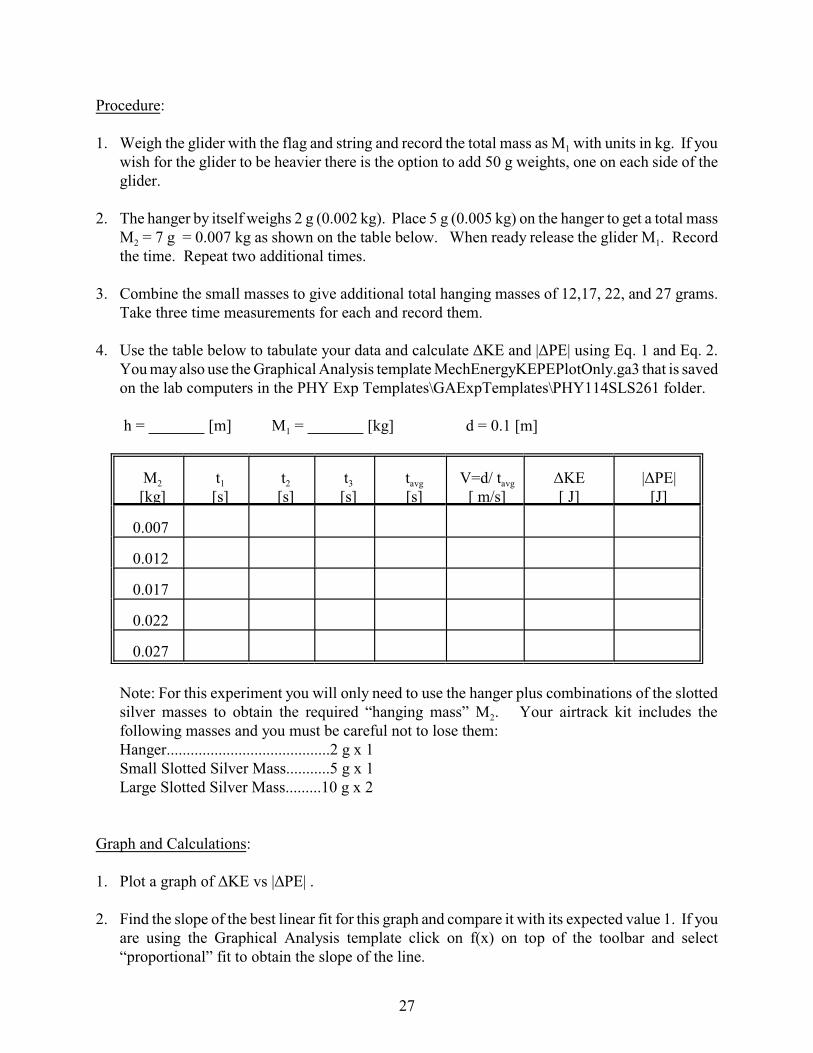
4. Use the table below to tabulate your data and calculate ÄKE and |ÄPE| using Eq. 1 and Eq. 2. You may also use the Graphical Analysis template MechEnergyKEPEPlotOnly.ga3 that is savedon the lab computers in the PHY Exp Templates\GAExpTemplates\PHY114SLS261 folder.

h = [m] M1 = [kg] d = 0.1 [m]

M2

[kg] t1

[s] t2

[s] t3

[s] tavg

[s]V=d/ tavg

[ m/s]ÄKE[ J]

|ÄPE|[J]

0.007

0.012

0.017

0.022

0.027

Note: For this experiment you will only need to use the hanger plus combinations of the slottedsilver masses to obtain the required “hanging mass” M2. Your airtrack kit includes thefollowing masses and you must be careful not to lose them:Hanger.........................................2 g x 1Small Slotted Silver Mass...........5 g x 1Large Slotted Silver Mass.........10 g x 2

Graph and Calculations:

1. Plot a graph of ÄKE vs |ÄPE| .

2. Find the slope of the best linear fit for this graph and compare it with its expected value 1. If youare using the Graphical Analysis template click on f(x) on top of the toolbar and select“proportional” fit to obtain the slope of the line.

27

Questions:

1. For a hanging weight of 8 g and a height of 2 m, make a prediction for the velocity of the glider.

2. Discuss possible deviations of the slope in cases when the airtrack was not leveled.

3. How would the slope (if compared to 1) of the best linear fit graph change in the presence offriction.

28

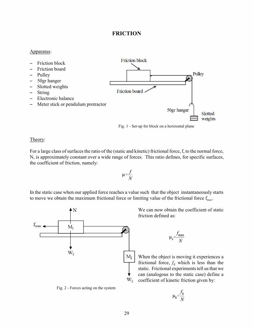
Fig. 1 - Set-up for block on a horizontal plane

Fig. 2 - Forces acting on the system

FRICTION

Apparatus:

S Friction blockS Friction boardS PulleyS 50gr hangerS Slotted weightsS StringS Electronic balanceS Meter stick or pendulum protractor

Theory:

For a large class of surfaces the ratio of the (static and kinetic) frictional force, f, to the normal force,N, is approximately constant over a wide range of forces. This ratio defines, for specific surfaces,the coefficient of friction, namely:

In the static case when our applied force reaches a value such that the object instantaneously startsto move we obtain the maximum frictional force or limiting value of the frictional force fmax.

We can now obtain the coefficient of staticfriction defined as:

When the object is moving it experiences africtional force, fK which is less than thestatic. Frictional experiments tell us that wecan (analogous to the static case) define acoefficient of kinetic friction given by:

29

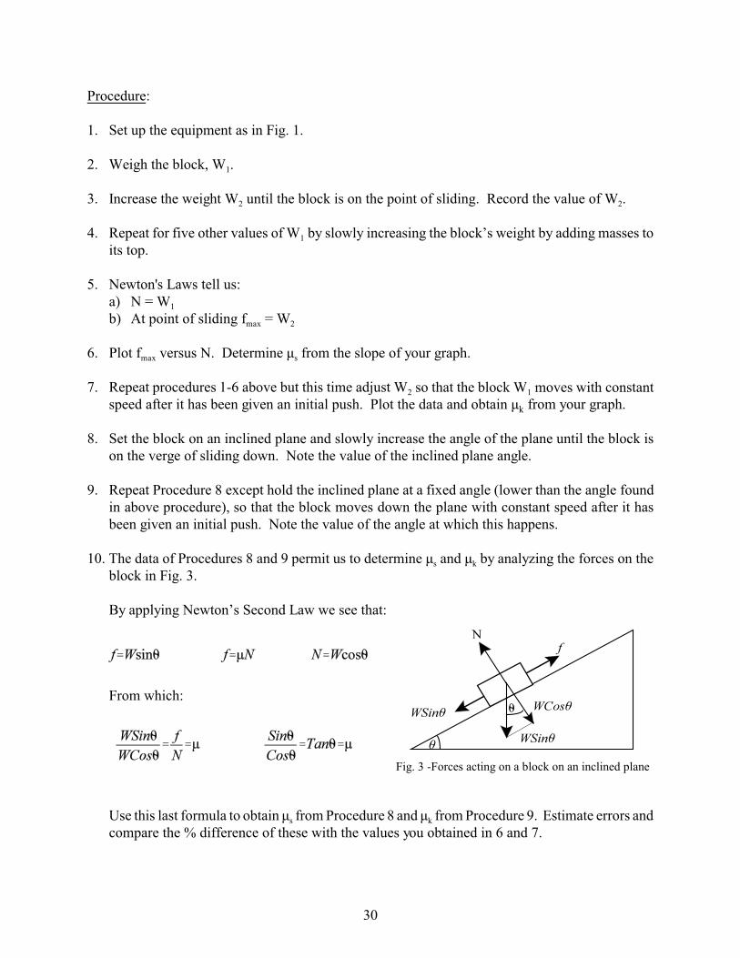
Fig. 3 -Forces acting on a block on an inclined plane

Procedure:

1. Set up the equipment as in Fig. 1.

2. Weigh the block, W1.

3. Increase the weight W2 until the block is on the point of sliding. Record the value of W2.

4. Repeat for five other values of W1 by slowly increasing the block’s weight by adding masses toits top.

5. Newton's Laws tell us: a) N = W1

b) At point of sliding fmax = W2

6. Plot fmax versus N. Determine ìs from the slope of your graph.

7. Repeat procedures 1-6 above but this time adjust W2 so that the block W1 moves with constantspeed after it has been given an initial push. Plot the data and obtain ìk from your graph.

8. Set the block on an inclined plane and slowly increase the angle of the plane until the block ison the verge of sliding down. Note the value of the inclined plane angle.

9. Repeat Procedure 8 except hold the inclined plane at a fixed angle (lower than the angle found

in above procedure), so that the block moves down the plane with constant speed after it hasbeen given an initial push. Note the value of the angle at which this happens.

10. The data of Procedures 8 and 9 permit us to determine ìs and ìk by analyzing the forces on theblock in Fig. 3.

By applying Newton’s Second Law we see that:

From which:

Use this last formula to obtain ìs from Procedure 8 and ìk from Procedure 9. Estimate errors andcompare the % difference of these with the values you obtained in 6 and 7.

30

Questions:

1. Which coefficient, ìs, or ìk is usually the larger?

2. What graphical curve should you obtain in part 6?

3. Is it possible to have a coefficient of friction greater than 1? Justify your answer.

31

32

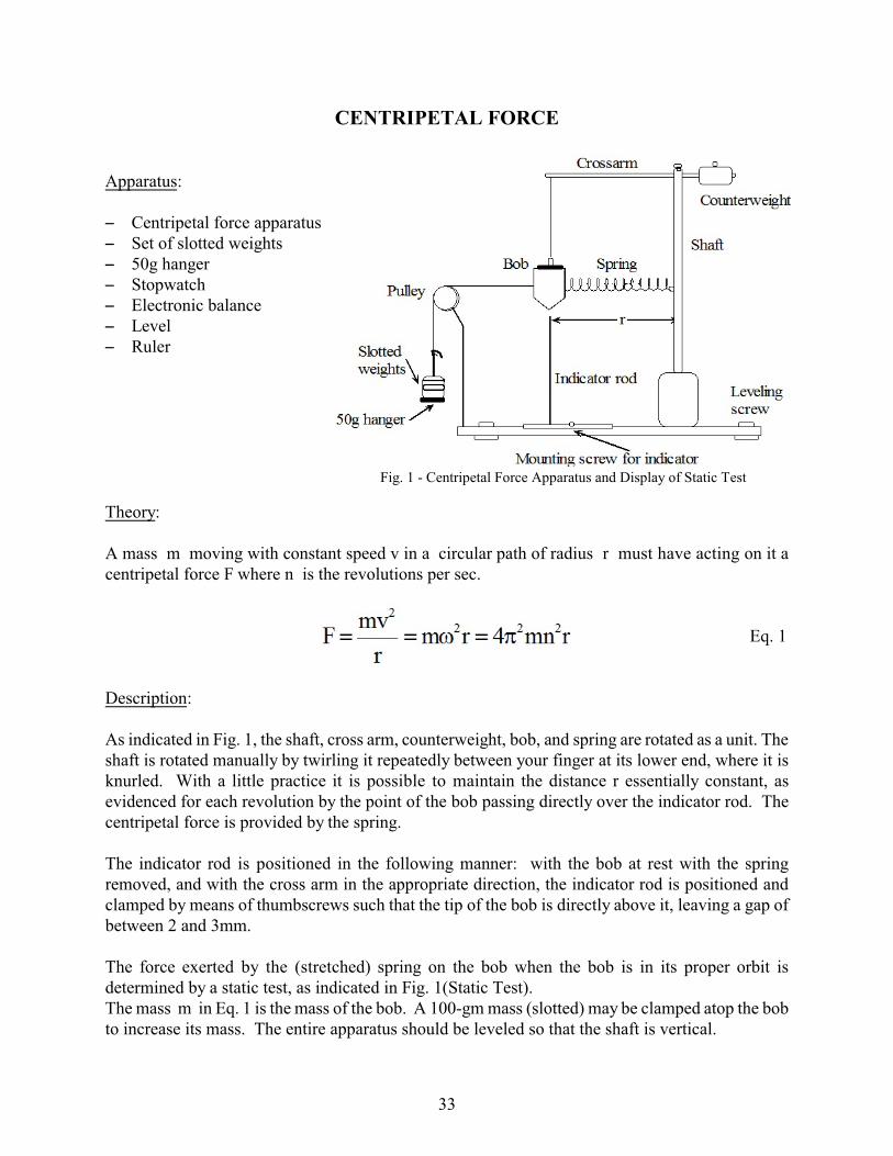
Fig. 1 - Centripetal Force Apparatus and Display of Static Test

CENTRIPETAL FORCE

Apparatus:

S Centripetal force apparatusS Set of slotted weightsS 50g hangerS StopwatchS Electronic balanceS Level S Ruler

Theory:

A mass m moving with constant speed v in a circular path of radius r must have acting on it acentripetal force F where n is the revolutions per sec.

Eq. 1

Description:

As indicated in Fig. 1, the shaft, cross arm, counterweight, bob, and spring are rotated as a unit. Theshaft is rotated manually by twirling it repeatedly between your finger at its lower end, where it isknurled. With a little practice it is possible to maintain the distance r essentially constant, asevidenced for each revolution by the point of the bob passing directly over the indicator rod. Thecentripetal force is provided by the spring.

The indicator rod is positioned in the following manner: with the bob at rest with the springremoved, and with the cross arm in the appropriate direction, the indicator rod is positioned andclamped by means of thumbscrews such that the tip of the bob is directly above it, leaving a gap ofbetween 2 and 3mm.

The force exerted by the (stretched) spring on the bob when the bob is in its proper orbit isdetermined by a static test, as indicated in Fig. 1(Static Test).The mass m in Eq. 1 is the mass of the bob. A 100-gm mass (slotted) may be clamped atop the bobto increase its mass. The entire apparatus should be leveled so that the shaft is vertical.

33

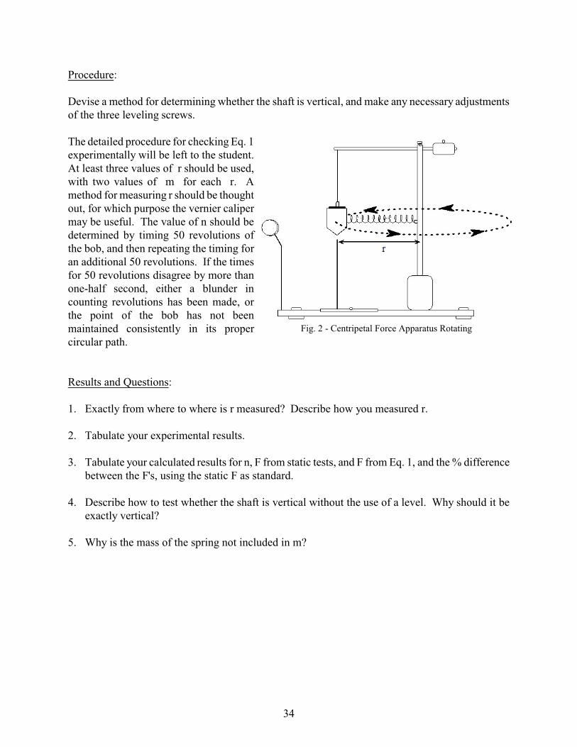
Fig. 2 - Centripetal Force Apparatus Rotating

Procedure:

Devise a method for determining whether the shaft is vertical, and make any necessary adjustmentsof the three leveling screws.

The detailed procedure for checking Eq. 1experimentally will be left to the student. At least three values of r should be used,with two values of m for each r. Amethod for measuring r should be thoughtout, for which purpose the vernier calipermay be useful. The value of n should bedetermined by timing 50 revolutions ofthe bob, and then repeating the timing foran additional 50 revolutions. If the timesfor 50 revolutions disagree by more thanone-half second, either a blunder incounting revolutions has been made, orthe point of the bob has not beenmaintained consistently in its propercircular path.

Results and Questions:

1. Exactly from where to where is r measured? Describe how you measured r.

2. Tabulate your experimental results. 3. Tabulate your calculated results for n, F from static tests, and F from Eq. 1, and the % difference

between the F's, using the static F as standard.

4. Describe how to test whether the shaft is vertical without the use of a level. Why should it beexactly vertical?

5. Why is the mass of the spring not included in m?

34

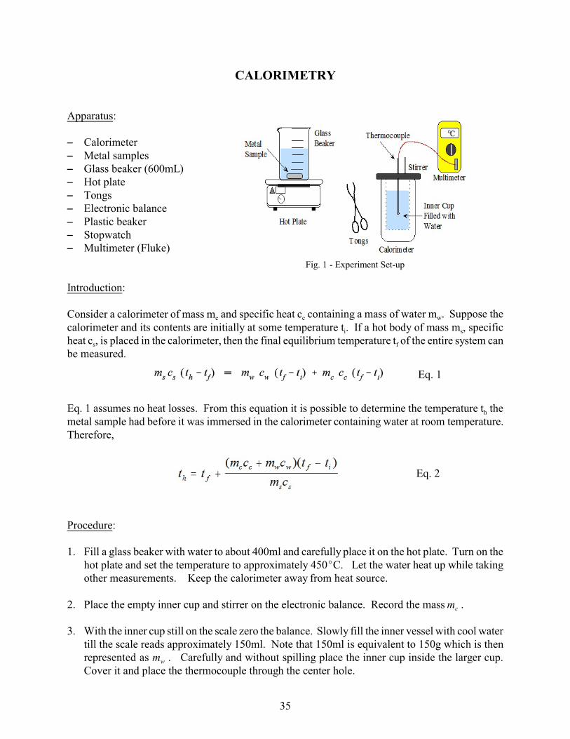
CALORIMETRY

Apparatus:

S CalorimeterS Metal samplesS Glass beaker (600mL)S Hot plateS TongsS Electronic balanceS Plastic beaker S StopwatchS Multimeter (Fluke)

Introduction:

Consider a calorimeter of mass mc and specific heat cc containing a mass of water mw. Suppose thecalorimeter and its contents are initially at some temperature ti. If a hot body of mass ms, specificheat cs, is placed in the calorimeter, then the final equilibrium temperature tf of the entire system canbe measured.

Eq. 1

Eq. 1 assumes no heat losses. From this equation it is possible to determine the temperature th themetal sample had before it was immersed in the calorimeter containing water at room temperature. Therefore,

Eq. 2

Procedure:

1. Fill a glass beaker with water to about 400ml and carefully place it on the hot plate. Turn on thehot plate and set the temperature to approximately 450EC. Let the water heat up while takingother measurements. Keep the calorimeter away from heat source.

2. Place the empty inner cup and stirrer on the electronic balance. Record the mass mc .

3. With the inner cup still on the scale zero the balance. Slowly fill the inner vessel with cool water till the scale reads approximately 150ml. Note that 150ml is equivalent to 150g which is thenrepresented as mw . Carefully and without spilling place the inner cup inside the larger cup. Cover it and place the thermocouple through the center hole.

Fig. 1 - Experiment Set-up

35

4. Obtain the mass of your metal sample.

5. Once the water starts to boil carefully place the metal sample in the beaker. Heat the samplefor10 minutes. While the sample is heating note the initial temperature of the water in thecalorimeter just prior to immersing the sample.

6. Immerse the hot sample in the calorimeter, cover it and stir gently. Note the final temperatureof the system after equilibrium has been reached.

7. Use Eq. 2 to calculate the temperature of the hot metal.

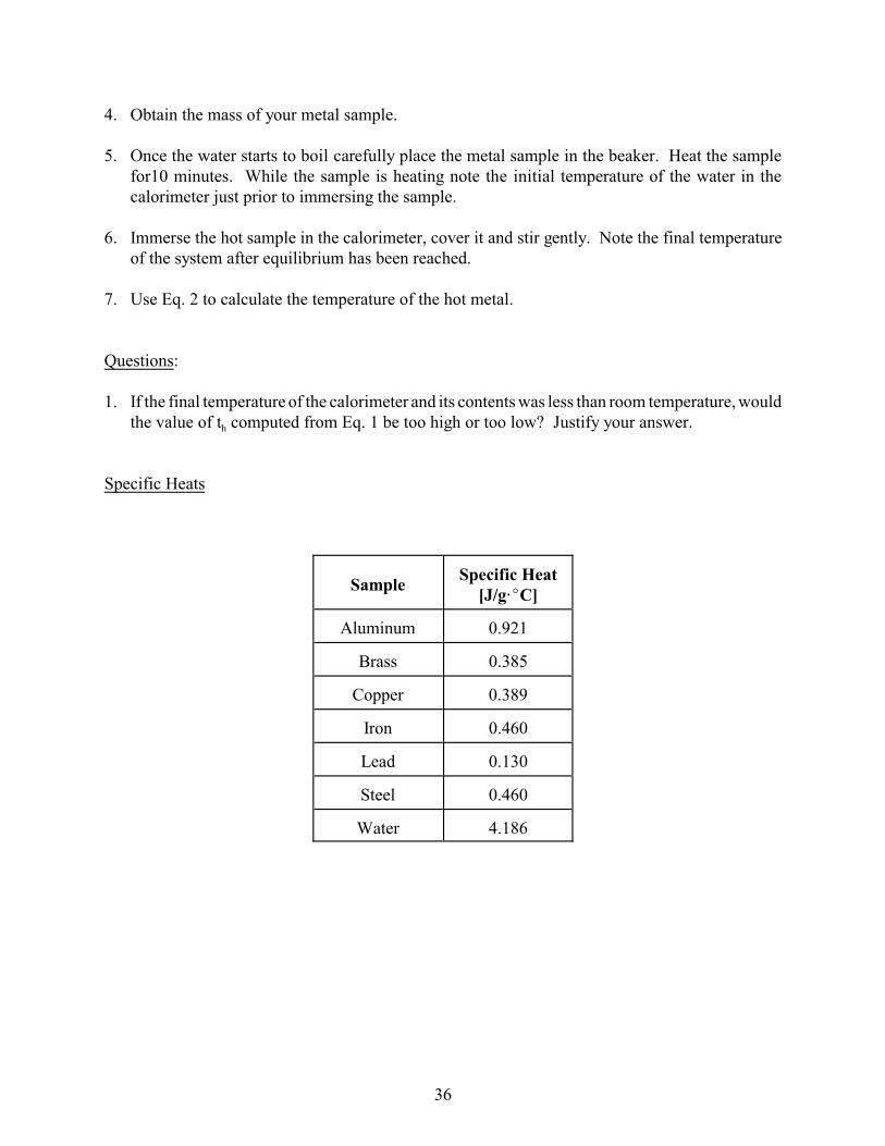
Questions:

1. If the final temperature of the calorimeter and its contents was less than room temperature, wouldthe value of th computed from Eq. 1 be too high or too low? Justify your answer.

Specific Heats

SampleSpecific Heat

[J/g@EC]

Aluminum 0.921

Brass 0.385

Copper 0.389

Iron 0.460

Lead 0.130

Steel 0.460

Water 4.186

36

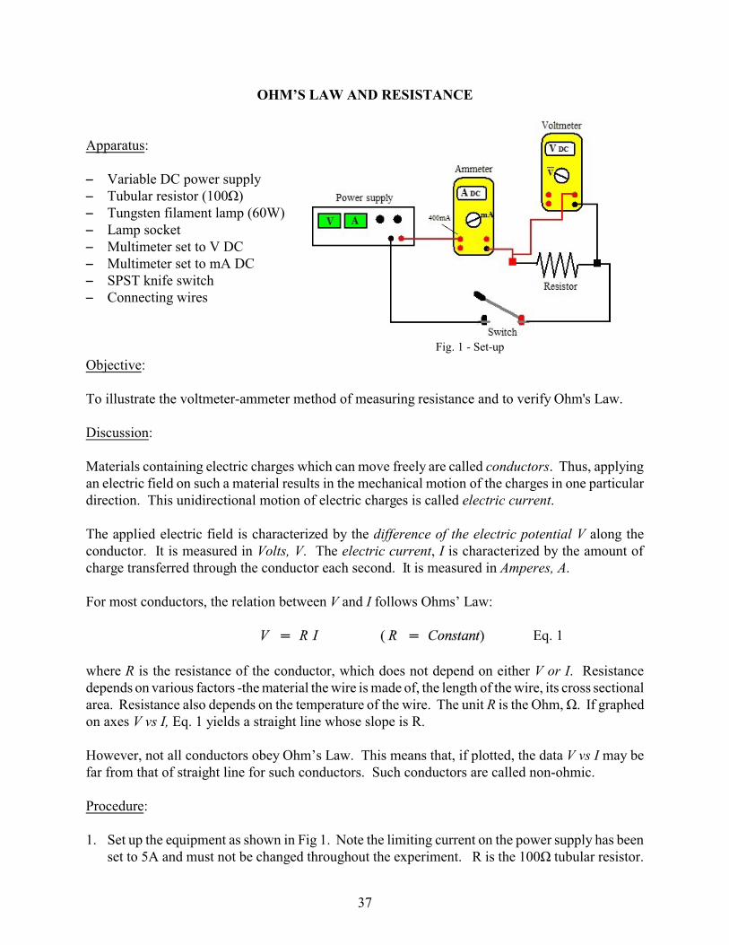
Fig. 1 - Set-up

OHM’S LAW AND RESISTANCE

Apparatus:

S Variable DC power supplyS Tubular resistor (100Ù)S Tungsten filament lamp (60W)S Lamp socketS Multimeter set to V DCS Multimeter set to mA DCS SPST knife switchS Connecting wires

Objective:

To illustrate the voltmeter-ammeter method of measuring resistance and to verify Ohm's Law.

Discussion:

Materials containing electric charges which can move freely are called conductors. Thus, applyingan electric field on such a material results in the mechanical motion of the charges in one particulardirection. This unidirectional motion of electric charges is called electric current.

The applied electric field is characterized by the difference of the electric potential V along theconductor. It is measured in Volts, V. The electric current, I is characterized by the amount ofcharge transferred through the conductor each second. It is measured in Amperes, A.

For most conductors, the relation between V and I follows Ohms’ Law:

Eq. 1

where R is the resistance of the conductor, which does not depend on either V or I. Resistancedepends on various factors -the material the wire is made of, the length of the wire, its cross sectionalarea. Resistance also depends on the temperature of the wire. The unit R is the Ohm, Ù. If graphedon axes V vs I, Eq. 1 yields a straight line whose slope is R.

However, not all conductors obey Ohm’s Law. This means that, if plotted, the data V vs I may befar from that of straight line for such conductors. Such conductors are called non-ohmic.

Procedure:

1. Set up the equipment as shown in Fig 1. Note the limiting current on the power supply has beenset to 5A and must not be changed throughout the experiment. R is the 100Ù tubular resistor.

37

The first multimeter will be used to measure the current I in your circuit, set it to mA and pressthe yellow key for DC Current. Set the second multimeter to VDC, this will measure the voltagedrop across the resistor. Have your instructor check your connections.Close the circuit and allow current to flow in the circuit. Set the power supply, Vo to 1, 2, 4, 6,10, 14, 18, 22, 26 and 30V and record the corresponding readings of I and V from themultimeters. When done, open the circuit.

2. With not current flowing through the circuit remove the tubular resistor and connect the tungstenlamp in its place. Have your instructor check your connections. Close the circuit and allow current to flow in the circuit. Set the power supply, Vo to 1, 2, 4, 6,10, 14, 18, 22, 26 and 30V and record the corresponding readings of I and V from themultimeters. Note that when using low voltages give it a few seconds to allow the current, I tostabilize before recording it. When done with the procedure, open the circuit and turn off all theinstruments.

Calculations and Graphs:

1. From the data of Procedure 1 plot V as the y-axis and I as the x-axis. If you obtain a straight linethen Ohm’s Law has been verified. Find the slope of the line and compare it to the knownresistance.

2. From the data of Procedure 2 plot V as the y-axis and I as the x-axis. Do you obtain a straightline or a parabolic curve?

Questions:

1. What is the accuracy of your measurements of R in Procedure 1?

2. What is your explanation for the fact that light bulb does not follow Ohm’s Law?

3. From the graph corresponding to the 60W bulb data find the current at 16V.

38

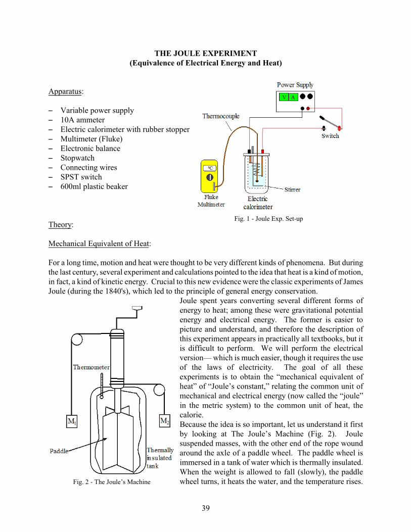
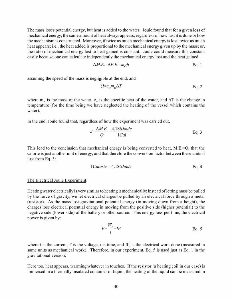
Fig. 2 - The Joule’s Machine

THE JOULE EXPERIMENT(Equivalence of Electrical Energy and Heat)

Apparatus:

S Variable power supplyS 10A ammeterS Electric calorimeter with rubber stopperS Multimeter (Fluke)S Electronic balanceS StopwatchS Connecting wiresS SPST switchS 600ml plastic beaker

Theory:

Mechanical Equivalent of Heat:

For a long time, motion and heat were thought to be very different kinds of phenomena. But duringthe last century, several experiment and calculations pointed to the idea that heat is a kind of motion,in fact, a kind of kinetic energy. Crucial to this new evidence were the classic experiments of JamesJoule (during the 1840's), which led to the principle of general energy conservation.

Joule spent years converting several different forms ofenergy to heat; among these were gravitational potentialenergy and electrical energy. The former is easier topicture and understand, and therefore the description ofthis experiment appears in practically all textbooks, but itis difficult to perform. We will perform the electricalversion— which is much easier, though it requires the useof the laws of electricity. The goal of all theseexperiments is to obtain the “mechanical equivalent ofheat” of “Joule’s constant,” relating the common unit ofmechanical and electrical energy (now called the “joule”in the metric system) to the common unit of heat, thecalorie.Because the idea is so important, let us understand it firstby looking at The Joule’s Machine (Fig. 2). Joulesuspended masses, with the other end of the rope woundaround the axle of a paddle wheel. The paddle wheel isimmersed in a tank of water which is thermally insulated. When the weight is allowed to fall (slowly), the paddlewheel turns, it heats the water, and the temperature rises.

Fig. 1 - Joule Exp. Set-up

39

Eq. 1

Eq. 2

Eq. 3

Eq. 4

Eq. 5

The mass loses potential energy, but heat is added to the water. Joule found that for a given loss ofmechanical energy, the same amount of heat always appears, regardless of how fast it is done or howthe mechanism is constructed. Moreover, if twice as much mechanical energy is lost, twice as muchheat appears; i.e., the heat added is proportional to the mechanical energy given up by the mass; or,the ratio of mechanical energy lost to heat gained is constant. Joule could measure this constanteasily because one can calculate independently the mechanical energy lost and the heat gained:

assuming the speed of the mass is negligible at the end, and

where mw is the mass of the water, cw is the specific heat of the water, and ÄT is the change intemperature (for the time being we have neglected the heating of the vessel which contains thewater).

In the end, Joule found that, regardless of how the experiment was carried out,

This lead to the conclusion that mechanical energy is being converted to heat, M.E.=Q, that thecalorie is just another unit of energy, and that therefore the conversion factor between these units ifjust from Eq. 3:

The Electrical Joule Experiment:

Heating water electrically is very similar to heating it mechanically: instead of letting mass be pulledby the force of gravity, we let electrical charges be pulled by an electrical force through a metal(resistor). As the mass lost gravitational potential energy (in moving down from a height), thecharges lose electrical potential energy in moving from the positive side (higher potential) to thenegative side (lower side) of the battery or other source. This energy loss per time, the electricalpower is given by:

where I is the current, V is the voltage, t is time, and We is the electrical work done (measured insame units as mechanical work). Therefore, in our experiment, Eq. 5 is used just as Eq. 1 in thegravitational version.

Here too, heat appears, warming whatever in touches. If the resistor (a heating coil in our case) isimmersed in a thermally insulated container of liquid, the heating of the liquid can be measured in

40

Eq. 6

the usual way, Eq. 2— except that for good accuracy one should include additional terms on the rightside to account for heat lost to the container and whatever else is warmed by the current (see Eq. 7). Thus, the ratio, J, is obtained here as W/Q.

We can do this for different amounts of electrical energy lost, and heat gained, simply by letting theheating take place for different lengths of time. And we can vary the rate of heating by changing thecurrent.

Procedure:

1. Using the electronic scale, weigh the inner cup of the calorimeter with the stirrer. Both must bedry. Denote the mass as mc .

2. Keep the inner cup on the scale and zero the latter. Fill the inner cup with approximately 250mlof cool water. Record the mass of the water as mw .

3. Carefully, place the inner vessel into the calorimeter, insert the heating coil. Place thethermocouple through the hole in the rubber stopper. Set the thermocouple so that it is insidethe coil not through it. The tip should be past the length of the coil but without touching thebottom.

4. Connect the circuit as shown on Fig. 1.

5. Turn on the power supply. Close the switch to allow current to run through the circuit. Slowlyset the voltage to 6V and record the corresponding current. Immediately, open the circuit toavoid heating the water before starting the experiment.

6. Turn on the multimeter and set to mV and press the yellow key to change the setting totemperature readouts. Stir the water, wait a bit for equilibrium, and record the temperature asTi this must be done before closing the circuit again.

7. When ready to start throw the switch to allow current to flow in the circuit again andsimultaneously start the timer.

8. Record the temperature at one minute intervals for 12 minutes or till water heats up to 10E to 15Eabove room temperature. During the process the water must be stirred constantly but gently.

Calculations:

You now have all the data to calculate, at each of the above points in time, the value of the Jouleconstant, J. From Eq. 5, obtain the energy dissipated by the coil:

41

Eq. 7

If I is in amperes, V in volts, and t in seconds, then We is in Joules.

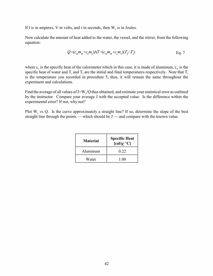
Now calculate the amount of heat added to the water, the vessel, and the stirrer, from the followingequation:

where cc is the specific heat of the calorimeter which in this case, it is made of aluminum, cw is thespecific heat of water and Ti and Tf are the initial and final temperatures respectively. Note that Ti

is the temperature you recorded in procedure 5, thus, it will remain the same throughout theexperiment and calculations.

Find the average of all values of J=We/Q thus obtained, and estimate your statistical error as outlinedby the instructor. Compare your average J with the accepted value. Is the difference within theexperimental error? If not, why not?

Plot We vs Q. Is the curve approximately a straight line? If so, determine the slope of the beststraight line through the points — which should be J — and compare with the known value.

MaterialSpecific Heat

[cal/g@EC]

Aluminum 0.22

Water 1.00

42

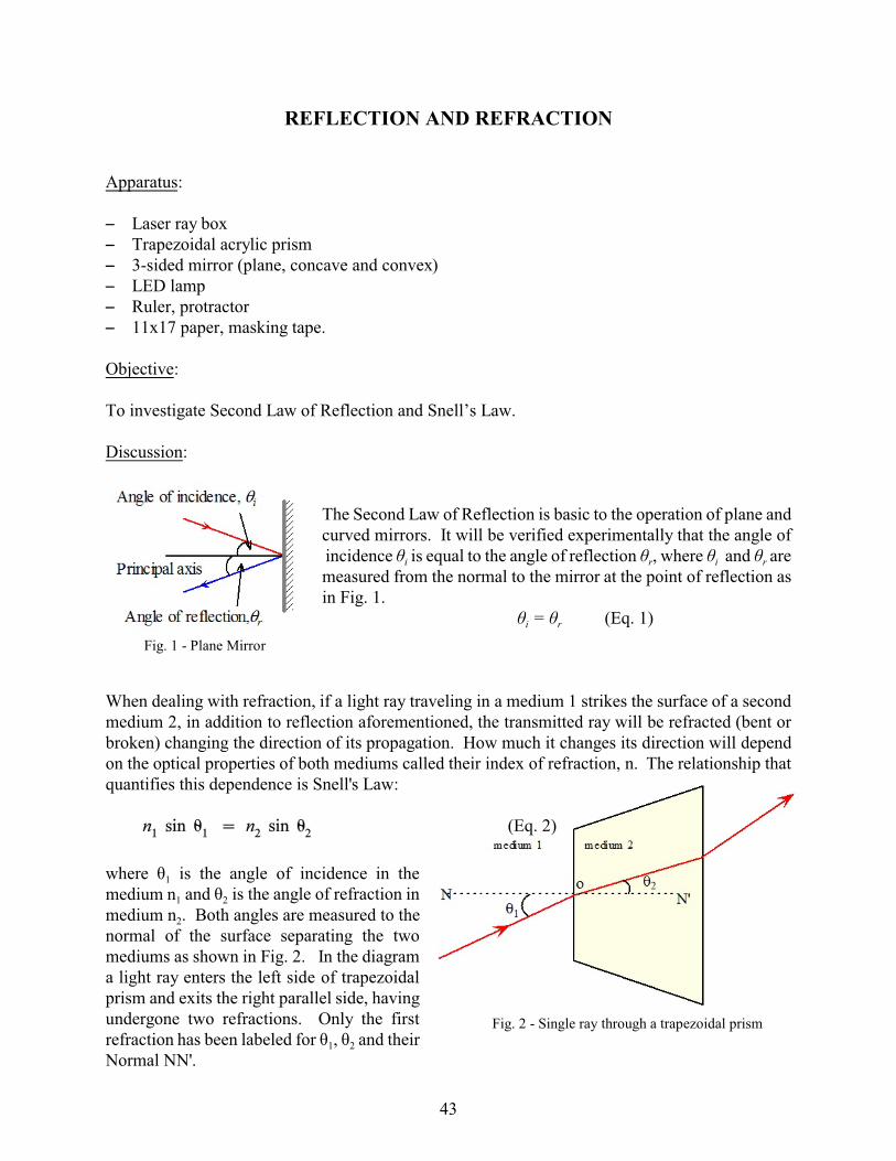
Fig. 1 - Plane Mirror

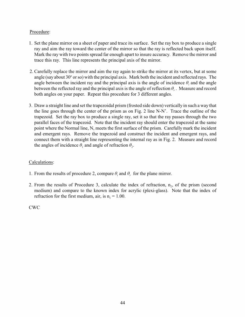
Fig. 2 - Single ray through a trapezoidal prism

REFLECTION AND REFRACTION

Apparatus:

S Laser ray boxS Trapezoidal acrylic prismS 3-sided mirror (plane, concave and convex)S LED lampS Ruler, protractorS 11x17 paper, masking tape.

Objective:

To investigate Second Law of Reflection and Snell’s Law.

Discussion:

The Second Law of Reflection is basic to the operation of plane and curved mirrors. It will be verified experimentally that the angle of incidence èi is equal to the angle of reflection èr, where èi and èr aremeasured from the normal to the mirror at the point of reflection asin Fig. 1.

èi = èr (Eq. 1)

When dealing with refraction, if a light ray traveling in a medium 1 strikes the surface of a secondmedium 2, in addition to reflection aforementioned, the transmitted ray will be refracted (bent orbroken) changing the direction of its propagation. How much it changes its direction will dependon the optical properties of both mediums called their index of refraction, n. The relationship thatquantifies this dependence is Snell's Law: (Eq. 2)

where è1 is the angle of incidence in themedium n1 and è2 is the angle of refraction inmedium n2. Both angles are measured to thenormal of the surface separating the twomediums as shown in Fig. 2. In the diagrama light ray enters the left side of trapezoidalprism and exits the right parallel side, havingundergone two refractions. Only the firstrefraction has been labeled for è1, è2 and theirNormal NN'.

43

Procedure:

1. Set the plane mirror on a sheet of paper and trace its surface. Set the ray box to produce a singleray and aim the ray toward the center of the mirror so that the ray is reflected back upon itself. Mark the ray with two points spread far enough apart to insure accuracy. Remove the mirror andtrace this ray. This line represents the principal axis of the mirror.

2. Carefully replace the mirror and aim the ray again to strike the mirror at its vertex, but at someangle (say about 30o or so) with the principal axis. Mark both the incident and reflected rays. Theangle between the incident ray and the principal axis is the angle of incidence èi and the anglebetween the reflected ray and the principal axis is the angle of reflection èr . Measure and recordboth angles on your paper. Repeat this procedure for 3 different angles.

3. Draw a straight line and set the trapezoidal prism (frosted side down) vertically in such a way thatthe line goes through the center of the prism as on Fig. 2 line N-N’. Trace the outline of thetrapezoid. Set the ray box to produce a single ray, set it so that the ray passes through the twoparallel faces of the trapezoid. Note that the incident ray should enter the trapezoid at the samepoint where the Normal line, N, meets the first surface of the prism. Carefully mark the incidentand emergent rays. Remove the trapezoid and construct the incident and emergent rays, andconnect them with a straight line representing the internal ray as in Fig. 2. Measure and recordthe angles of incidence è1 and angle of refraction è2.

Calculations:

1. From the results of procedure 2, compare èi and èr for the plane mirror.

2. From the results of Procedure 3, calculate the index of refraction, n2, of the prism (secondmedium) and compare to the known index for acrylic (plexi-glass). Note that the index ofrefraction for the first medium, air, is n1 = 1.00.

CWC

44

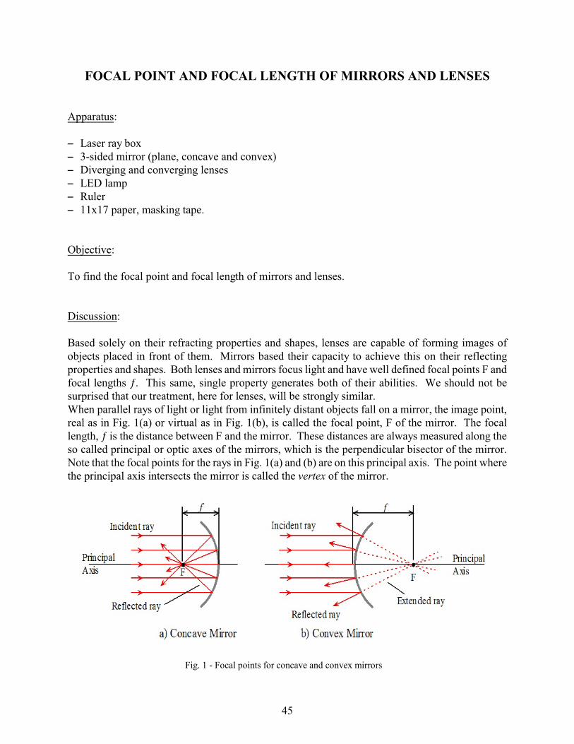
Fig. 1 - Focal points for concave and convex mirrors

FOCAL POINT AND FOCAL LENGTH OF MIRRORS AND LENSES

Apparatus:

S Laser ray boxS 3-sided mirror (plane, concave and convex)S Diverging and converging lensesS LED lampS RulerS 11x17 paper, masking tape.

Objective:

To find the focal point and focal length of mirrors and lenses.

Discussion:

Based solely on their refracting properties and shapes, lenses are capable of forming images ofobjects placed in front of them. Mirrors based their capacity to achieve this on their reflectingproperties and shapes. Both lenses and mirrors focus light and have well defined focal points F andfocal lengths ƒ. This same, single property generates both of their abilities. We should not besurprised that our treatment, here for lenses, will be strongly similar.When parallel rays of light or light from infinitely distant objects fall on a mirror, the image point,real as in Fig. 1(a) or virtual as in Fig. 1(b), is called the focal point, F of the mirror. The focallength, ƒ is the distance between F and the mirror. These distances are always measured along theso called principal or optic axes of the mirrors, which is the perpendicular bisector of the mirror.Note that the focal points for the rays in Fig. 1(a) and (b) are on this principal axis. The point wherethe principal axis intersects the mirror is called the vertex of the mirror.

45

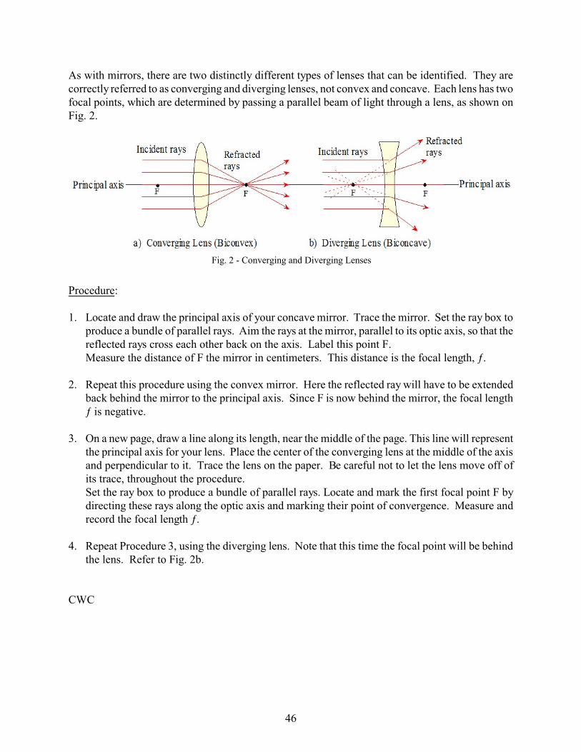
Fig. 2 - Converging and Diverging Lenses

As with mirrors, there are two distinctly different types of lenses that can be identified. They arecorrectly referred to as converging and diverging lenses, not convex and concave. Each lens has twofocal points, which are determined by passing a parallel beam of light through a lens, as shown onFig. 2.

Procedure:

1. Locate and draw the principal axis of your concave mirror. Trace the mirror. Set the ray box to produce a bundle of parallel rays. Aim the rays at the mirror, parallel to its optic axis, so that thereflected rays cross each other back on the axis. Label this point F.Measure the distance of F the mirror in centimeters. This distance is the focal length, ƒ.

2. Repeat this procedure using the convex mirror. Here the reflected ray will have to be extendedback behind the mirror to the principal axis. Since F is now behind the mirror, the focal lengthƒ is negative.

3. On a new page, draw a line along its length, near the middle of the page. This line will representthe principal axis for your lens. Place the center of the converging lens at the middle of the axisand perpendicular to it. Trace the lens on the paper. Be careful not to let the lens move off ofits trace, throughout the procedure.Set the ray box to produce a bundle of parallel rays. Locate and mark the first focal point F bydirecting these rays along the optic axis and marking their point of convergence. Measure andrecord the focal length ƒ.

4. Repeat Procedure 3, using the diverging lens. Note that this time the focal point will be behindthe lens. Refer to Fig. 2b.

CWC

46

Eq. 1

SOUND WAVES

Apparatus:

S 1000ml graduated cylinderS Acrylic tubeS Tuning forks (various frequencies)S Rubber activator

Objective:

To determine the wavelengths in air of sound waves of different frequencies by the method ofresonance in closed pipes and to calculate the speed of sound in air using these measurements.

Discussion:

The speed of sound can be measured directly by timing the passage of a sound over a long, knowndistance. To do this with an ordinary watch requires a much longer distance than is available in thelaboratory. It is convenient, therefore, to resort to an indirect way of measuring the speed of soundin air by making use of its wave properties. For all waves the following relationship holds: where v is the speed of the wave, f is its frequency of vibration, and ë is its wavelength. In this

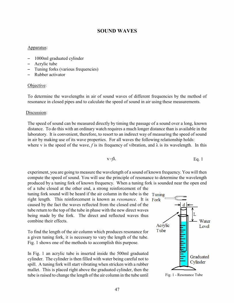
experiment, you are going to measure the wavelength of a sound of known frequency. You will thencompute the speed of sound. You will use the principle of resonance to determine the wavelengthproduced by a tuning fork of known frequency. When a tuning fork is sounded near the open end of a tube closed at the other end, a strong reinforcement of thetuning fork sound will be heard if the air column in the tube is theright length. This reinforcement is known as resonance. It iscaused by the fact the waves reflected from the closed end of thetube return to the top of the tube in phase with the new direct wavesbeing made by the fork. The direct and reflected waves thuscombine their effects.

To find the length of the air column which produces resonance fora given tuning fork, it is necessary to vary the length of the tube. Fig. 1 shows one of the methods to accomplish this purpose.

In Fig. 1 an acrylic tube is inserted inside the 500ml graduatedcylinder. The cylinder is then filled with water being careful not tospill. A tuning fork will start vibrating when stricken with a rubbermallet. This is placed right above the graduated cylinder, then thetube is raised to change the length of the air column in the tube until Fig. 1 - Resonance Tube

47

Eq. 2

the sound intensity is at a maximum. For a tube closed at one end, whose diameter is smallcompared to its length, strong resonance will occur when the length of the air column is one-quarterof a wavelength, ë/4, of the sound waves made by the tuning fork. A less intense resonance will alsobe heard when the tube length is 3/4ë, 5/4ë, and so on.Since the shortest tube length for which resonance occurs is L=ë/4, it follows that ë. Practically, thisrelationship must be corrected for the diameter d of the tube. This gives:

In this experiment ë, L, and d will be measured in meters.

Procedure:

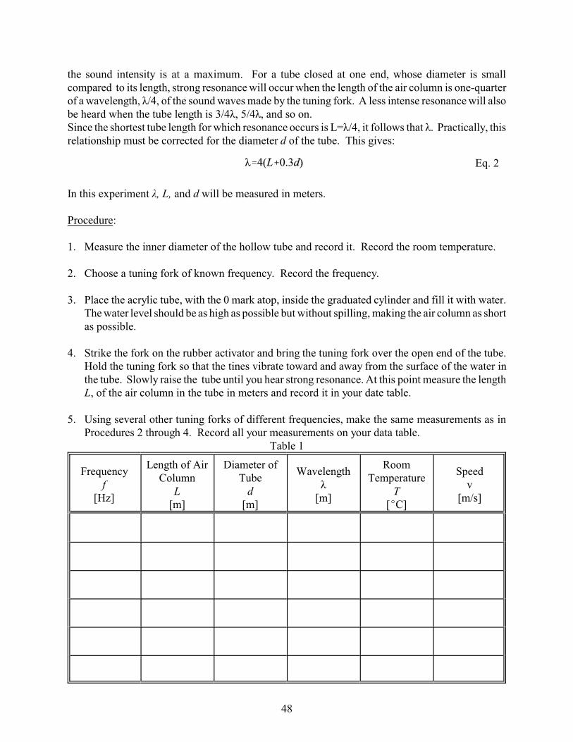
1. Measure the inner diameter of the hollow tube and record it. Record the room temperature.

2. Choose a tuning fork of known frequency. Record the frequency.

3. Place the acrylic tube, with the 0 mark atop, inside the graduated cylinder and fill it with water.The water level should be as high as possible but without spilling, making the air column as shortas possible.

4. Strike the fork on the rubber activator and bring the tuning fork over the open end of the tube. Hold the tuning fork so that the tines vibrate toward and away from the surface of the water inthe tube. Slowly raise the tube until you hear strong resonance. At this point measure the lengthL, of the air column in the tube in meters and record it in your date table.

5. Using several other tuning forks of different frequencies, make the same measurements as inProcedures 2 through 4. Record all your measurements on your data table.

Table 1

Frequencyf

[Hz]

Length of AirColumn

L[m]

Diameter ofTube

d[m]

Wavelengthë

[m]

RoomTemperature

T[EC]

Speedv

[m/s]

48

Eq. 3

Calculations:

1. Using the values of L and d in Table 1, calculate the value of the wavelength ë from Eq. 2. Enterthis value of wavelength in the table.

2. Using Eq. 1 calculate the value of the speed of sound in air and record this value in the table foreach of the tuning forks used.

3. Calculate the value of the speed of sound in air from the following relation:

where T is the temperature in degrees centigrade and 331m/s is the speed of sound in air at 0EC.

4. Compare the result obtained by resonance measurement with the calculated value obtained byusing Eq. 3.

Questions:

1. How could you use the method and the results of this experiment to determine whether the speedof sound in air depends upon its frequency? What do your results indicate about such arelationship?

2. If we assume that the speed of sound at any temperature is known from Eq. 3, how can thisexperiment be used to measure the frequency of an unmarked tuning fork?

49

50

SUPPLEMENTARYEXPERIMENTS

51

52

Eq. 1

Eq. 2

Eq. 3

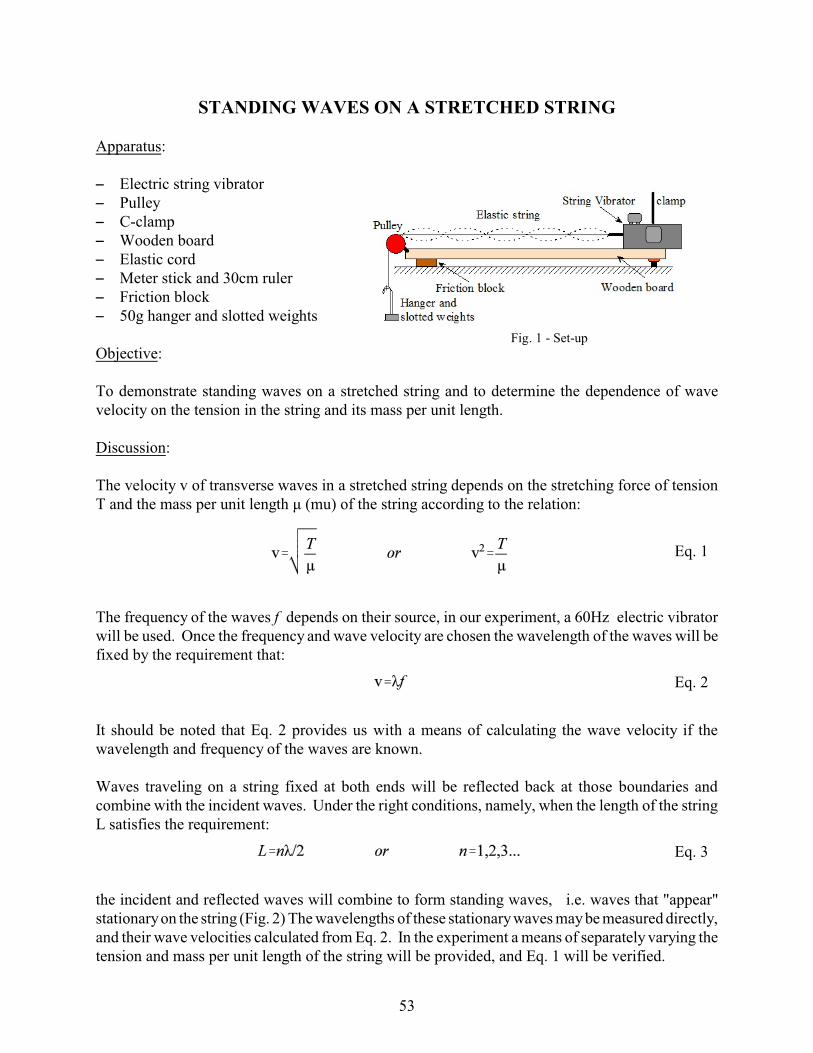
STANDING WAVES ON A STRETCHED STRING

Apparatus:

S Electric string vibratorS PulleyS C-clampS Wooden boardS Elastic cordS Meter stick and 30cm rulerS Friction blockS 50g hanger and slotted weights

Objective:

To demonstrate standing waves on a stretched string and to determine the dependence of wavevelocity on the tension in the string and its mass per unit length.

Discussion:

The velocity v of transverse waves in a stretched string depends on the stretching force of tensionT and the mass per unit length ì (mu) of the string according to the relation:

The frequency of the waves f depends on their source, in our experiment, a 60Hz electric vibratorwill be used. Once the frequency and wave velocity are chosen the wavelength of the waves will befixed by the requirement that:

It should be noted that Eq. 2 provides us with a means of calculating the wave velocity if thewavelength and frequency of the waves are known.

Waves traveling on a string fixed at both ends will be reflected back at those boundaries andcombine with the incident waves. Under the right conditions, namely, when the length of the stringL satisfies the requirement:

the incident and reflected waves will combine to form standing waves, i.e. waves that "appear"stationary on the string (Fig. 2) The wavelengths of these stationary waves may be measured directly,and their wave velocities calculated from Eq. 2. In the experiment a means of separately varying thetension and mass per unit length of the string will be provided, and Eq. 1 will be verified.

Fig. 1 - Set-up

53

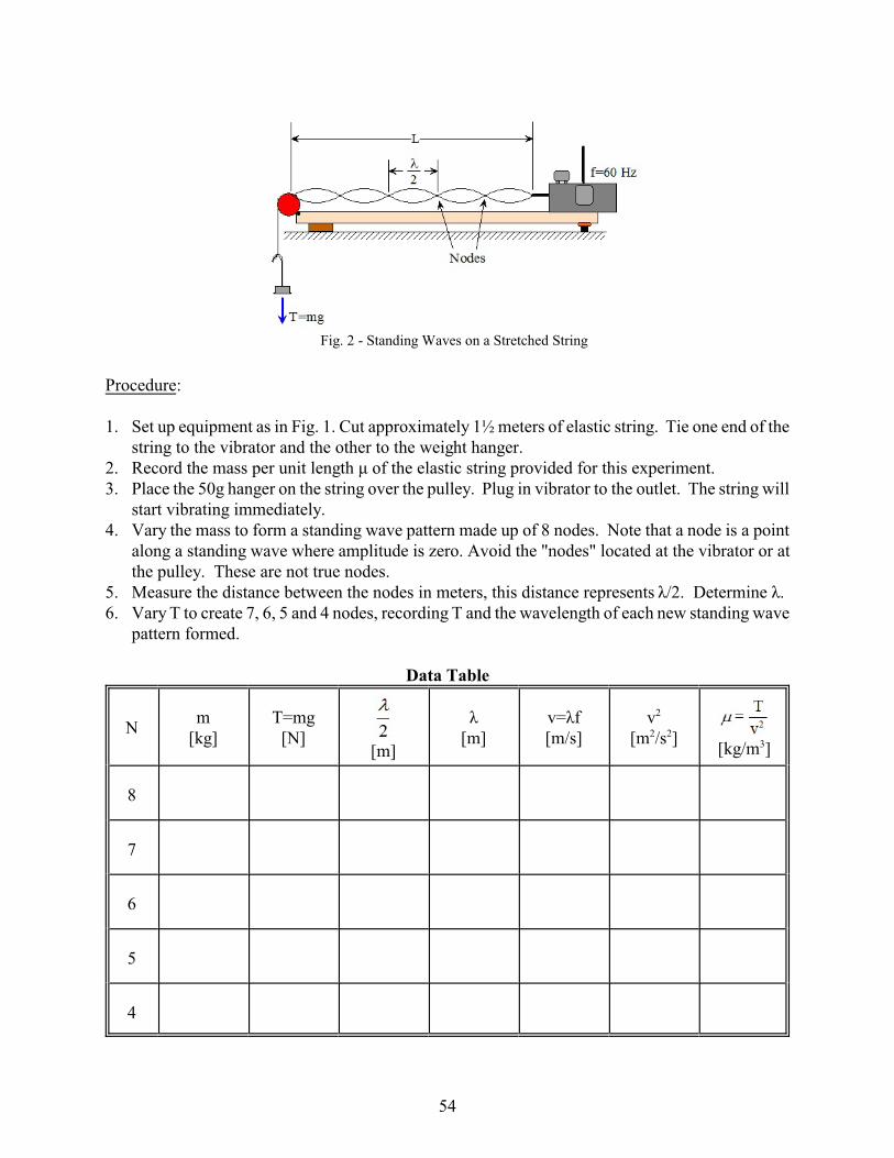
Procedure:

1. Set up equipment as in Fig. 1. Cut approximately 1½ meters of elastic string. Tie one end of thestring to the vibrator and the other to the weight hanger.

2. Record the mass per unit length ì of the elastic string provided for this experiment. 3. Place the 50g hanger on the string over the pulley. Plug in vibrator to the outlet. The string will

start vibrating immediately. 4. Vary the mass to form a standing wave pattern made up of 8 nodes. Note that a node is a point

along a standing wave where amplitude is zero. Avoid the "nodes" located at the vibrator or atthe pulley. These are not true nodes.

5. Measure the distance between the nodes in meters, this distance represents ë/2. Determine ë.6. Vary T to create 7, 6, 5 and 4 nodes, recording T and the wavelength of each new standing wave

pattern formed.

Data Table

Nm

[kg]T=mg

[N][m]

ë[m]

v=ëf[m/s]

v2

[m2/s2][kg/m3]

8

7

6

5

4

Fig. 2 - Standing Waves on a Stretched String

54

Calculations:

1. Calculate tension T = mg.2. Obtain the wavelength ë in meters.3. Calculate velocity using Eq. 2 where f=60Hz. 4. Plot T as ordinate against v2 as abscissa. Fit the plotted data with a straight line that passes

through the origin. Record the slope and compare to the known value of ì.5. Use Eq. 1 to determine ì for each set of nodes. Calculate the average of ì and compare to the

known value of ì.

55

56

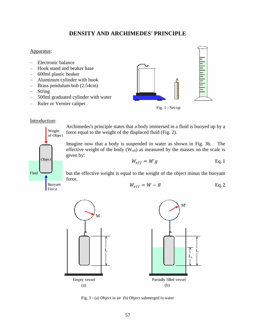
57

DENSITY AND ARCHIMEDES' PRINCIPLE

Apparatus:

‒ Electronic balance

‒ Hook stand and beaker base

‒ 600ml plastic beaker

‒ Aluminum cylinder with hook

‒ Brass pendulum bob (2.54cm)

‒ String

‒ 500ml graduated cylinder with water

‒ Ruler or Vernier caliper

Introduction:

Archimedes's principle states that a body immersed in a fluid is buoyed up by a

force equal to the weight of the displaced fluid (Fig. 2).

Imagine now that a body is suspended in water as shown in Fig. 3b. The

effective weight of the body (Weff) as measured by the masses on the scale is

given by:

𝑊𝑒𝑓𝑓 = 𝑀′𝑔 Eq. 1

but the effective weight is equal to the weight of the object minus the buoyant

force.

𝑊𝑒𝑓𝑓 = 𝑊 − 𝐵 Eq. 2

Fig. 3 - (a) Object in air (b) Object submerged in water

Buoyant

Force

Weight

of Object

Fluid

Object

L

Li

M

Empty vessel

L

M'

Partially filled vessel

(a) (b)

Fig. 1 - Set-up

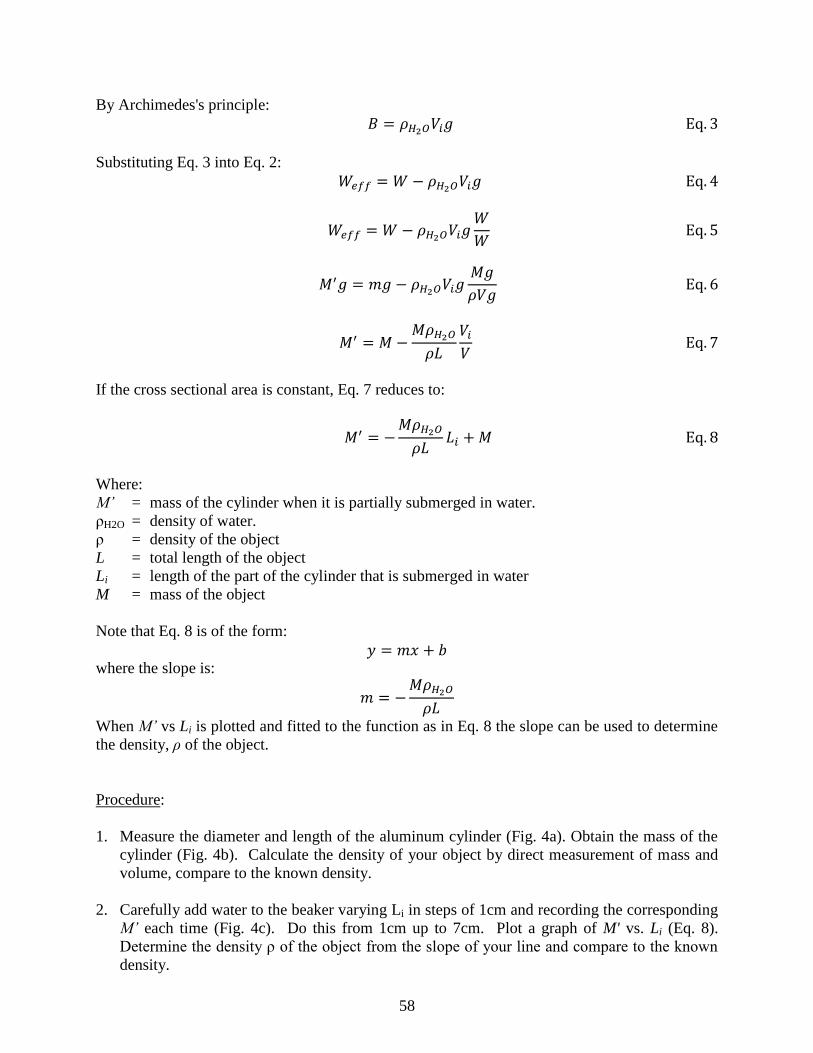
58

By Archimedes's principle:

𝐵 = 𝜌𝐻2𝑂𝑉𝑖𝑔 Eq. 3

Substituting Eq. 3 into Eq. 2:

𝑊𝑒𝑓𝑓 = 𝑊 − 𝜌𝐻2𝑂𝑉𝑖𝑔 Eq. 4

𝑊𝑒𝑓𝑓 = 𝑊 − 𝜌𝐻2𝑂𝑉𝑖𝑔𝑊

𝑊 Eq. 5

𝑀′𝑔 = 𝑚𝑔 − 𝜌𝐻2𝑂𝑉𝑖𝑔𝑀𝑔

𝜌𝑉𝑔 Eq. 6

𝑀′ = 𝑀 −𝑀𝜌𝐻2𝑂

𝜌𝐿

𝑉𝑖

𝑉 Eq. 7

If the cross sectional area is constant, Eq. 7 reduces to:

𝑀′ = −𝑀𝜌𝐻2𝑂

𝜌𝐿𝐿𝑖 + 𝑀 Eq. 8

Where:

M’ = mass of the cylinder when it is partially submerged in water.

ρH2O = density of water.

ρ = density of the object

L = total length of the object

Li = length of the part of the cylinder that is submerged in water

M = mass of the object

Note that Eq. 8 is of the form:

𝑦 = 𝑚𝑥 + 𝑏 where the slope is:

𝑚 = −𝑀𝜌𝐻2𝑂

𝜌𝐿

When M’ vs Li is plotted and fitted to the function as in Eq. 8 the slope can be used to determine

the density, ρ of the object.

Procedure:

1. Measure the diameter and length of the aluminum cylinder (Fig. 4a). Obtain the mass of the

cylinder (Fig. 4b). Calculate the density of your object by direct measurement of mass and

volume, compare to the known density.

2. Carefully add water to the beaker varying Li in steps of 1cm and recording the corresponding

M’ each time (Fig. 4c). Do this from 1cm up to 7cm. Plot a graph of M' vs. Li (Eq. 8).

Determine the density ρ of the object from the slope of your line and compare to the known

density.

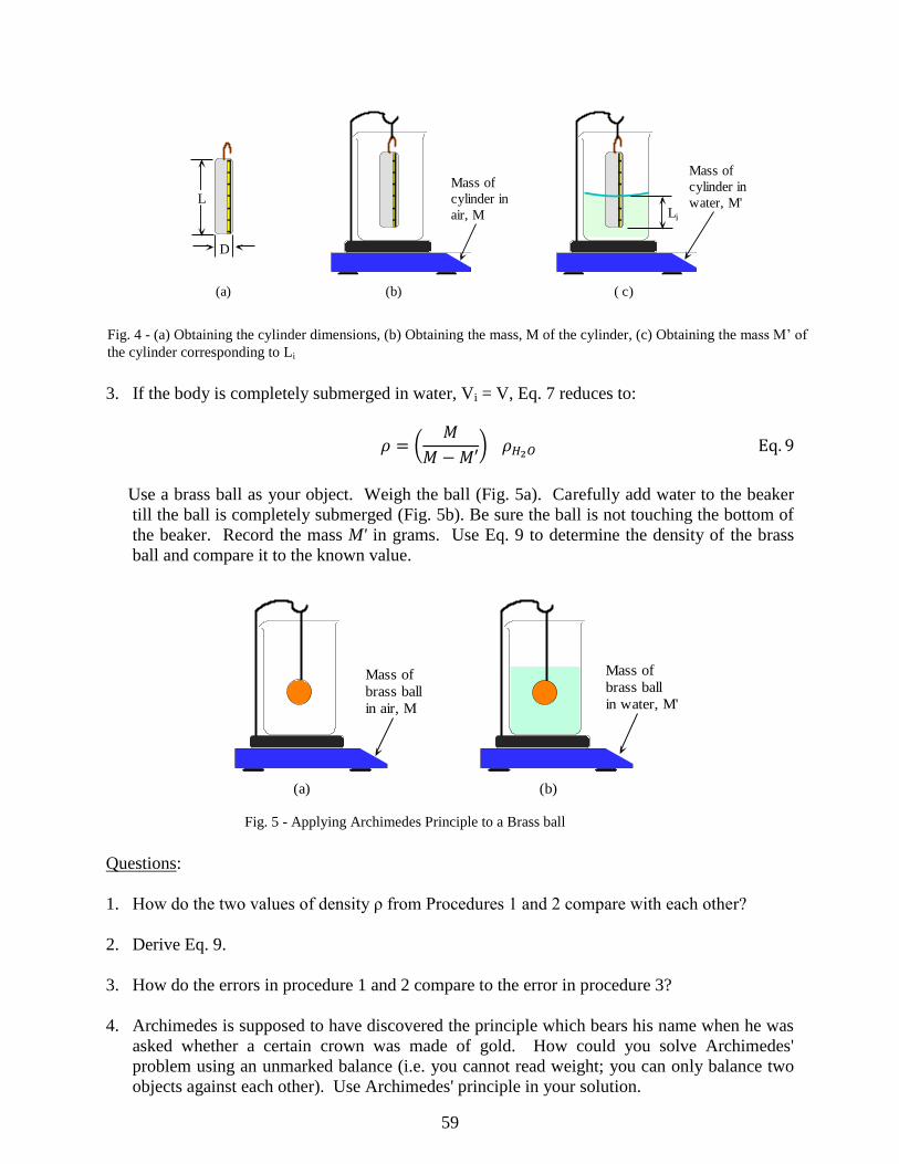
59

3. If the body is completely submerged in water, Vi = V, Eq. 7 reduces to:

𝜌 = (𝑀

𝑀 − 𝑀′) 𝜌𝐻2𝑂 Eq. 9

Use a brass ball as your object. Weigh the ball (Fig. 5a). Carefully add water to the beaker

till the ball is completely submerged (Fig. 5b). Be sure the ball is not touching the bottom of

the beaker. Record the mass M' in grams. Use Eq. 9 to determine the density of the brass

ball and compare it to the known value.

Questions:

1. How do the two values of density ρ from Procedures 1 and 2 compare with each other?

2. Derive Eq. 9.

3. How do the errors in procedure 1 and 2 compare to the error in procedure 3?

4. Archimedes is supposed to have discovered the principle which bears his name when he was

asked whether a certain crown was made of gold. How could you solve Archimedes'

problem using an unmarked balance (i.e. you cannot read weight; you can only balance two

objects against each other). Use Archimedes' principle in your solution.

D

L

Mass of

cylinder in

air, M Li

Mass of

cylinder in

water, M'

(a) (b) ( c)

Fig. 4 - (a) Obtaining the cylinder dimensions, (b) Obtaining the mass, M of the cylinder, (c) Obtaining the mass M’ of

the cylinder corresponding to Li

Mass of

brass ball

in air, M

Mass of

brass ball

in water, M'

(a) (b)

Fig. 5 - Applying Archimedes Principle to a Brass ball

60

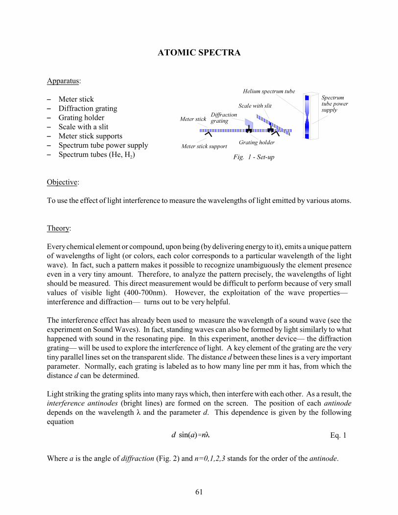
Eq. 1

ATOMIC SPECTRA

Apparatus:

S Meter stickS Diffraction gratingS Grating holderS Scale with a slitS Meter stick supportsS Spectrum tube power supplyS Spectrum tubes (He, H2)

Objective:

To use the effect of light interference to measure the wavelengths of light emitted by various atoms.

Theory:

Every chemical element or compound, upon being (by delivering energy to it), emits a unique pattern of wavelengths of light (or colors, each color corresponds to a particular wavelength of the lightwave). In fact, such a pattern makes it possible to recognize unambiguously the element presenceeven in a very tiny amount. Therefore, to analyze the pattern precisely, the wavelengths of lightshould be measured. This direct measurement would be difficult to perform because of very smallvalues of visible light (400-700nm). However, the exploitation of the wave properties— interference and diffraction— turns out to be very helpful.

The interference effect has already been used to measure the wavelength of a sound wave (see theexperiment on Sound Waves). In fact, standing waves can also be formed by light similarly to whathappened with sound in the resonating pipe. In this experiment, another device— the diffractiongrating— will be used to explore the interference of light. A key element of the grating are the verytiny parallel lines set on the transparent slide. The distance d between these lines is a very importantparameter. Normally, each grating is labeled as to how many line per mm it has, from which thedistance d can be determined.

Light striking the grating splits into many rays which, then interfere with each other. As a result, theinterference antinodes (bright lines) are formed on the screen. The position of each antinodedepends on the wavelength ë and the parameter d. This dependence is given by the followingequation

Where a is the angle of diffraction (Fig. 2) and n=0,1,2,3 stands for the order of the antinode.

61

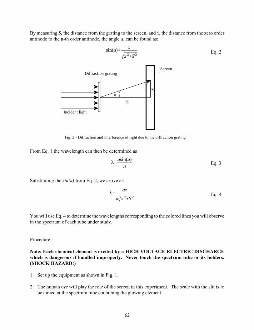
Eq. 2

Fig. 2 - Diffraction and interference of light due to the diffraction grating

Eq. 3

Eq. 4

By measuring S, the distance from the grating to the screen, and x, the distance from the zero orderantinode to the n-th order antinode, the angle a, can be found as:

From Eq. 1 the wavelength can then be determined as

Substituting the sin(a) from Eq. 2, we arrive at:

You will use Eq. 4 to determine the wavelengths corresponding to the colored lines you will observein the spectrum of each tube under study.

Procedure:

Note: Each chemical element is excited by a HIGH VOLTAGE ELECTRIC DISCHARGEwhich is dangerous if handled improperly. Never touch the spectrum tube or its holders.(SHOCK HAZARD!)

1. Set up the equipment as shown in Fig. 1.

2. The human eye will play the role of the screen in this experiment. The scale with the slit is tobe aimed at the spectrum tube containing the glowing element.

62

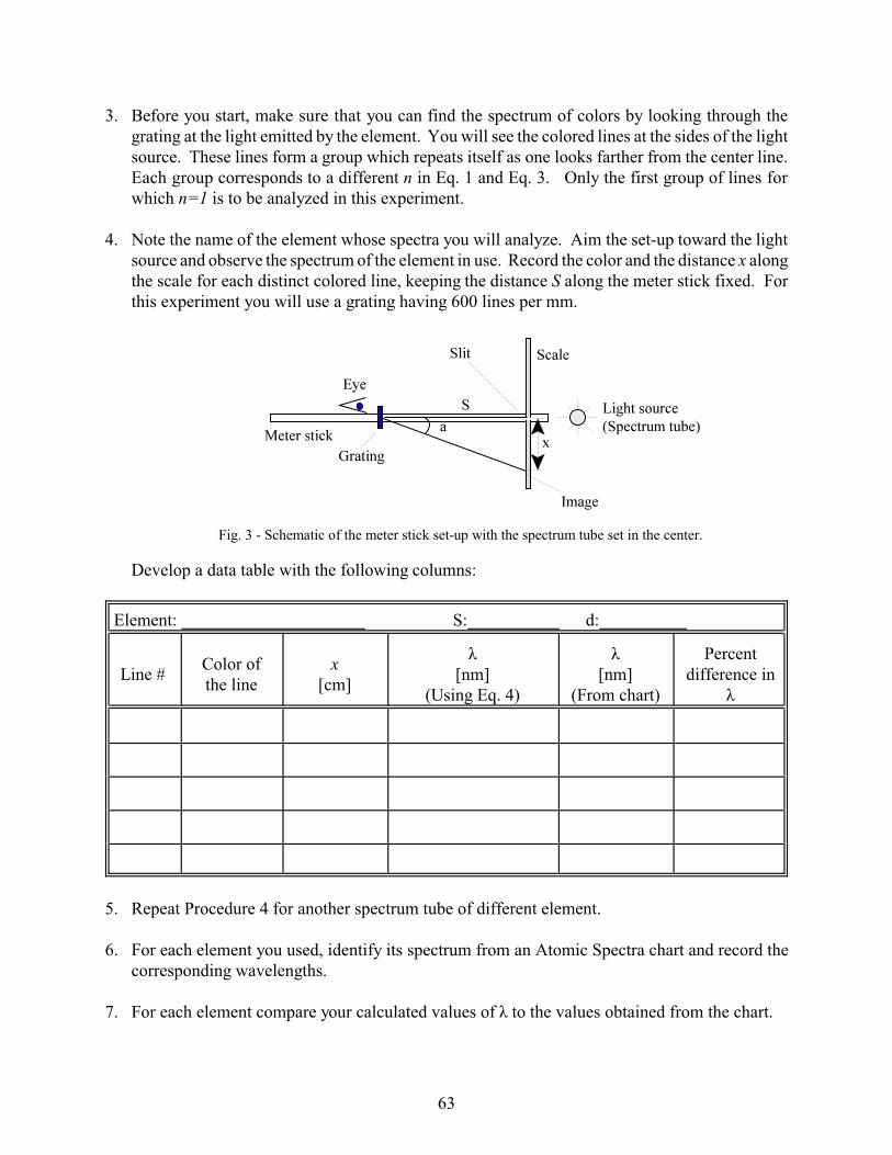
Fig. 3 - Schematic of the meter stick set-up with the spectrum tube set in the center.

3. Before you start, make sure that you can find the spectrum of colors by looking through thegrating at the light emitted by the element. You will see the colored lines at the sides of the lightsource. These lines form a group which repeats itself as one looks farther from the center line. Each group corresponds to a different n in Eq. 1 and Eq. 3. Only the first group of lines forwhich n=1 is to be analyzed in this experiment.

4. Note the name of the element whose spectra you will analyze. Aim the set-up toward the lightsource and observe the spectrum of the element in use. Record the color and the distance x alongthe scale for each distinct colored line, keeping the distance S along the meter stick fixed. Forthis experiment you will use a grating having 600 lines per mm.

Develop a data table with the following columns:

Element: S: d:

Line #Color ofthe line

x[cm]

ë[nm]

(Using Eq. 4)

ë[nm]

(From chart)

Percentdifference in

ë

5. Repeat Procedure 4 for another spectrum tube of different element.

6. For each element you used, identify its spectrum from an Atomic Spectra chart and record the corresponding wavelengths.

7. For each element compare your calculated values of ë to the values obtained from the chart.

63

64

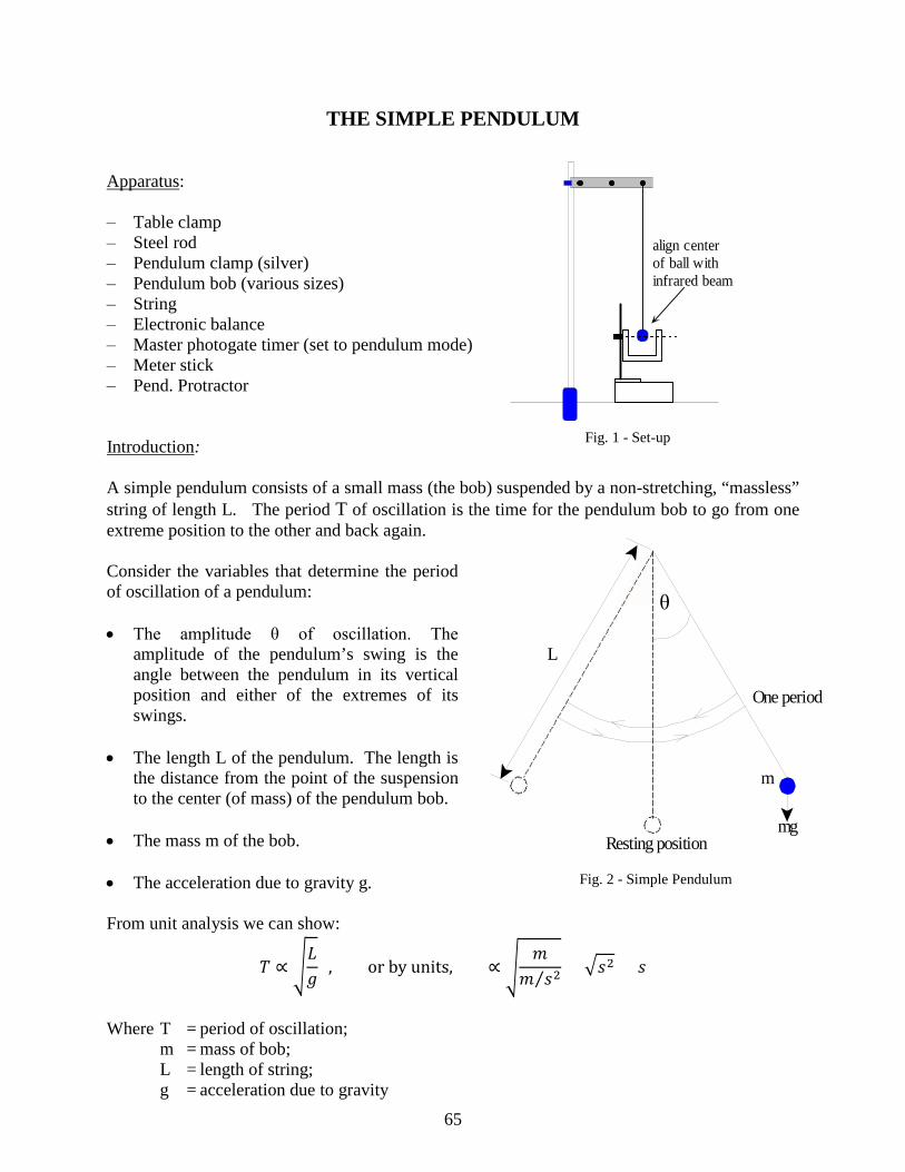
65

THE SIMPLE PENDULUM Apparatus

:

‒ Table clamp ‒ Steel rod ‒ Pendulum clamp (silver) ‒ Pendulum bob (various sizes) ‒ String ‒ Electronic balance ‒ Master photogate timer (set to pendulum mode) ‒ Meter stick ‒ Pend. Protractor Introduction

:

A simple pendulum consists of a small mass (the bob) suspended by a non-stretching, “massless” string of length L. The period T of oscillation is the time for the pendulum bob to go from one extreme position to the other and back again. Consider the variables that determine the period of oscillation of a pendulum: • The amplitude θ of oscillation. The

amplitude of the pendulum’s swing is the angle between the pendulum in its vertical position and either of the extremes of its swings.

• The length L of the pendulum. The length is

the distance from the point of the suspension to the center (of mass) of the pendulum bob.

• The mass m of the bob. • The acceleration due to gravity g. From unit analysis we can show:

𝑇 ∝ 𝐿𝑔

, or by units, ∝ 𝑚

𝑚 𝑠2⁄ = 𝑠2 = 𝑠

Where T = period of oscillation; m = mass of bob; L = length of string; g = acceleration due to gravity

align centerof ball withinfrared beam

Fig. 1 - Set-up

L

θ

m

mgResting position

One period

Fig. 2 - Simple Pendulum

66

Since an oscillation is described mathematically by cos ωt and knowing that ω=2πf where f = 1/T we then have:

𝑇 =2𝜋𝜔

Eq. 1 Equation 1 can be re-writen as:

𝑇 = 2𝜋𝐿𝑔

Eq. 2

Procedure

:

Make the following measurements: 1. Turn on the photogate and set it to pendulum mode. In addition, make sure the memory

switch on as well. Set-up the pendulum so that when it is in resting position it blocks the photogate as shown on Fig. 1.

2. Period as a function of amplitude (plot T vs. θ). Perform this procedure for amplitudes of

5° to 30° in steps of 5°. The length and mass will remain constant. At each given angle allow the pendulum to swing through the photogate, be careful not to strike the photogate with the pendulum. Record the period displayed on the photogate that corresponds to the amplitude.

3. Period as a function of length (plot T vs. L). Use a small angle such as 10°. Change the

length 6 times. Each time a new length L is set, the length must be measured from the center of the bob to the pivot point. The amplitude and the mass will remain constant. Allow the pendulum to swing through the photogate and record the period displayed on the photogate. Fit the data to Eq. 2. How does the obtained “g” value from the fit compare to the known value of “g”?

Note: An alternate method for this procedure is to plot T2 vs L and use the best linear fit to determine the slope. Then use the slope to obtain g and compare to the known value. The linear fit would be of the form: 𝑇2 = 4𝜋

𝑔𝐿.

4. Period as a function of mass (plot T vs. m). Use a small angle such as 10°. Use 4

different masses but keep amplitude and length constant. For each mass record the period as displayed on the photogate.

Questions

:

1. For the simple pendulum where is the maximum for: displacement, velocity and acceleration?

2. Would the period increase or decrease if the experiments were held on : a) the top of a high mountain? b) the moon? c) on Jupiter?

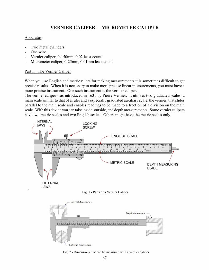
Fig. 1 - Parts of a Vernier Caliper

Fig. 2 - Dimensions that can be measured with a vernier caliper

ENGLISH SCALE

VERNIER CALIPER - MICROMETER CALIPER

Apparatus:

- Two metal cylinders- One wire- Vernier caliper, 0-150mm, 0.02 least count- Micrometer caliper, 0-25mm, 0.01mm least count

Part I: The Vernier Caliper

When you use English and metric rulers for making measurements it is sometimes difficult to getprecise results. When it is necessary to make more precise linear measurements, you must have amore precise instrument. One such instrument is the vernier caliper. The vernier caliper was introduced in 1631 by Pierre Vernier. It utilizes two graduated scales: amain scale similar to that of a ruler and a especially graduated auxiliary scale, the vernier, that slidesparallel to the main scale and enables readings to be made to a fraction of a division on the mainscale. With this device you can take inside, outside, and depth measurements. Some vernier calipershave two metric scales and two English scales. Others might have the metric scales only.

67

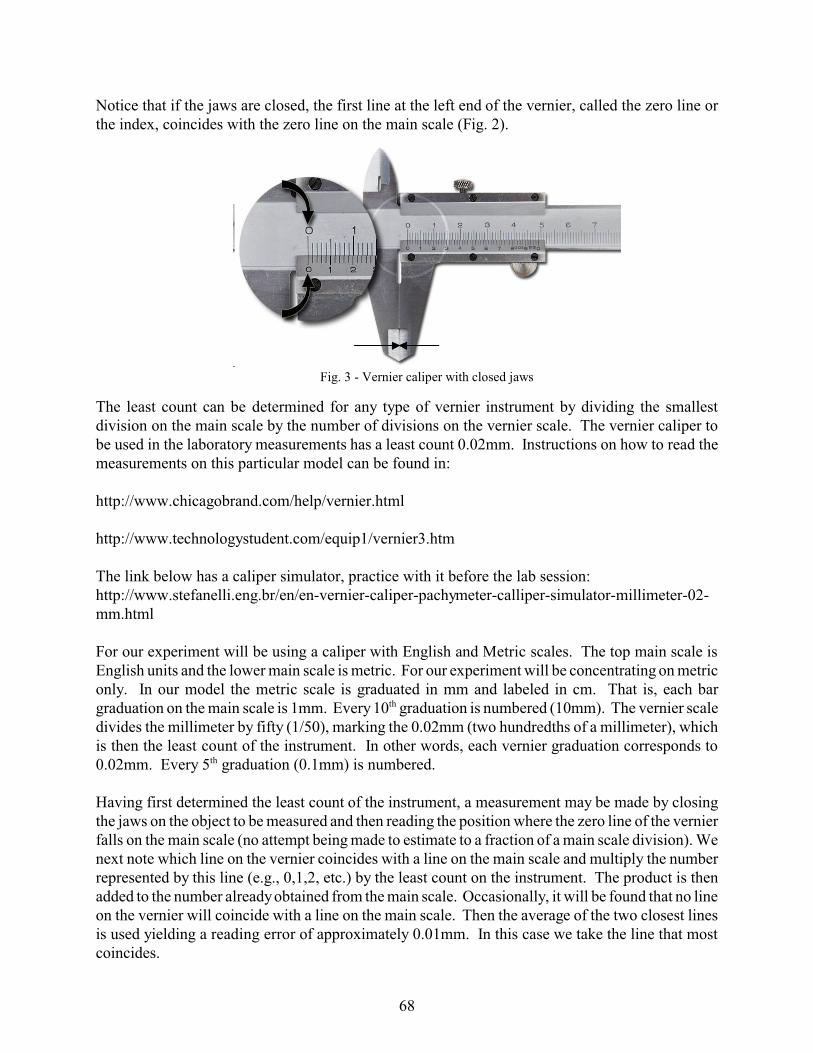
Fig. 3 - Vernier caliper with closed jaws

Notice that if the jaws are closed, the first line at the left end of the vernier, called the zero line orthe index, coincides with the zero line on the main scale (Fig. 2).

The least count can be determined for any type of vernier instrument by dividing the smallestdivision on the main scale by the number of divisions on the vernier scale. The vernier caliper tobe used in the laboratory measurements has a least count 0.02mm. Instructions on how to read themeasurements on this particular model can be found in:

http://www.chicagobrand.com/help/vernier.html

http://www.technologystudent.com/equip1/vernier3.htm

The link below has a caliper simulator, practice with it before the lab session:http://www.stefanelli.eng.br/en/en-vernier-caliper-pachymeter-calliper-simulator-millimeter-02-mm.html

For our experiment will be using a caliper with English and Metric scales. The top main scale isEnglish units and the lower main scale is metric. For our experiment will be concentrating on metriconly. In our model the metric scale is graduated in mm and labeled in cm. That is, each bargraduation on the main scale is 1mm. Every 10th graduation is numbered (10mm). The vernier scaledivides the millimeter by fifty (1/50), marking the 0.02mm (two hundredths of a millimeter), whichis then the least count of the instrument. In other words, each vernier graduation corresponds to0.02mm. Every 5th graduation (0.1mm) is numbered.

Having first determined the least count of the instrument, a measurement may be made by closingthe jaws on the object to be measured and then reading the position where the zero line of the vernierfalls on the main scale (no attempt being made to estimate to a fraction of a main scale division). Wenext note which line on the vernier coincides with a line on the main scale and multiply the numberrepresented by this line (e.g., 0,1,2, etc.) by the least count on the instrument. The product is thenadded to the number already obtained from the main scale. Occasionally, it will be found that no lineon the vernier will coincide with a line on the main scale. Then the average of the two closest linesis used yielding a reading error of approximately 0.01mm. In this case we take the line that mostcoincides.

68

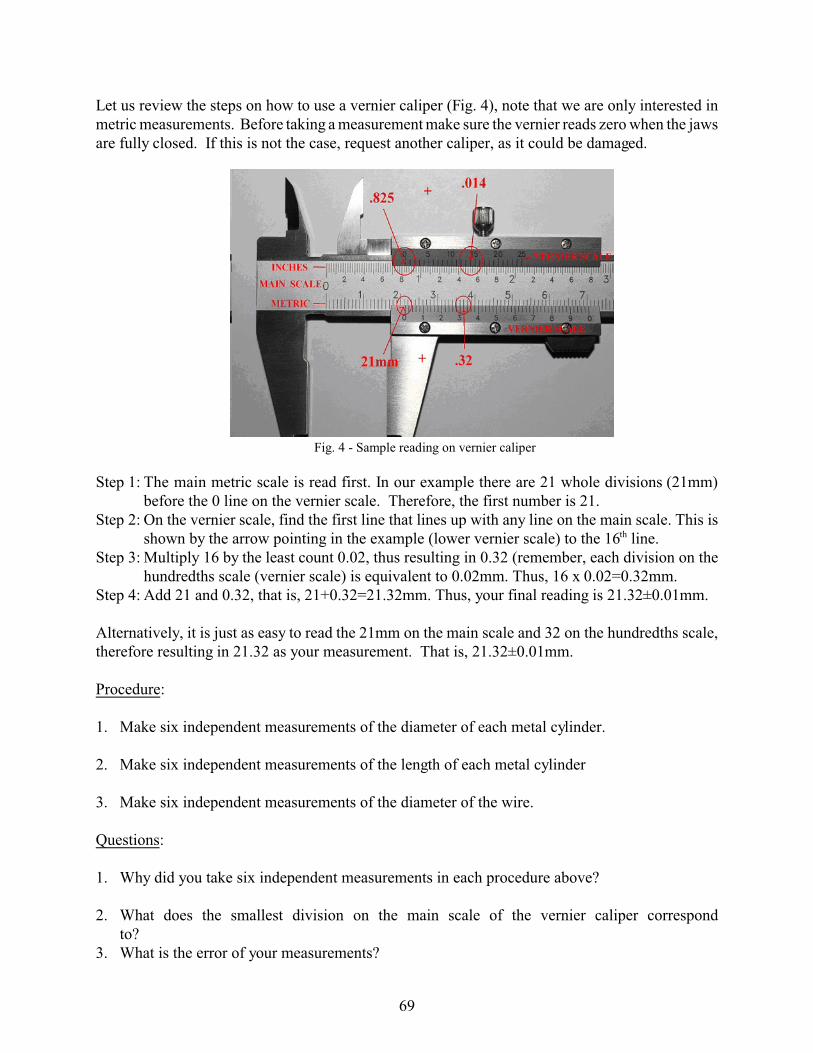
Fig. 4 - Sample reading on vernier caliper

Let us review the steps on how to use a vernier caliper (Fig. 4), note that we are only interested inmetric measurements. Before taking a measurement make sure the vernier reads zero when the jawsare fully closed. If this is not the case, request another caliper, as it could be damaged.

Step 1: The main metric scale is read first. In our example there are 21 whole divisions (21mm)before the 0 line on the vernier scale. Therefore, the first number is 21.

Step 2: On the vernier scale, find the first line that lines up with any line on the main scale. This isshown by the arrow pointing in the example (lower vernier scale) to the 16th line.

Step 3: Multiply 16 by the least count 0.02, thus resulting in 0.32 (remember, each division on thehundredths scale (vernier scale) is equivalent to 0.02mm. Thus, 16 x 0.02=0.32mm.

Step 4: Add 21 and 0.32, that is, 21+0.32=21.32mm. Thus, your final reading is 21.32±0.01mm.

Alternatively, it is just as easy to read the 21mm on the main scale and 32 on the hundredths scale,therefore resulting in 21.32 as your measurement. That is, 21.32±0.01mm.

Procedure:

1. Make six independent measurements of the diameter of each metal cylinder.

2. Make six independent measurements of the length of each metal cylinder

3. Make six independent measurements of the diameter of the wire.

Questions:

1. Why did you take six independent measurements in each procedure above?

2. What does the smallest division on the main scale of the vernier caliper correspond to?

3. What is the error of your measurements?

69

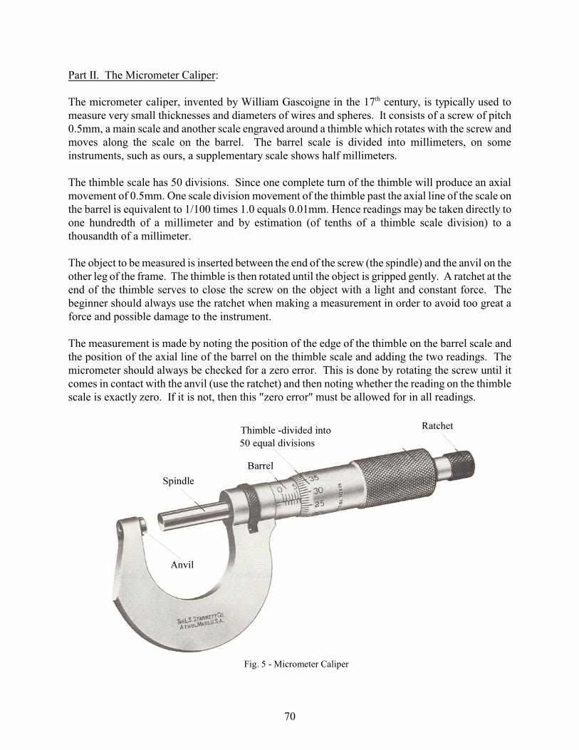
Fig. 5 - Micrometer Caliper

Part II. The Micrometer Caliper:

The micrometer caliper, invented by William Gascoigne in the 17th century, is typically used tomeasure very small thicknesses and diameters of wires and spheres. It consists of a screw of pitch0.5mm, a main scale and another scale engraved around a thimble which rotates with the screw andmoves along the scale on the barrel. The barrel scale is divided into millimeters, on someinstruments, such as ours, a supplementary scale shows half millimeters.

The thimble scale has 50 divisions. Since one complete turn of the thimble will produce an axialmovement of 0.5mm. One scale division movement of the thimble past the axial line of the scale onthe barrel is equivalent to 1/100 times 1.0 equals 0.01mm. Hence readings may be taken directly toone hundredth of a millimeter and by estimation (of tenths of a thimble scale division) to athousandth of a millimeter.

The object to be measured is inserted between the end of the screw (the spindle) and the anvil on theother leg of the frame. The thimble is then rotated until the object is gripped gently. A ratchet at theend of the thimble serves to close the screw on the object with a light and constant force. Thebeginner should always use the ratchet when making a measurement in order to avoid too great aforce and possible damage to the instrument.

The measurement is made by noting the position of the edge of the thimble on the barrel scale andthe position of the axial line of the barrel on the thimble scale and adding the two readings. Themicrometer should always be checked for a zero error. This is done by rotating the screw until itcomes in contact with the anvil (use the ratchet) and then noting whether the reading on the thimblescale is exactly zero. If it is not, then this "zero error" must be allowed for in all readings.

70

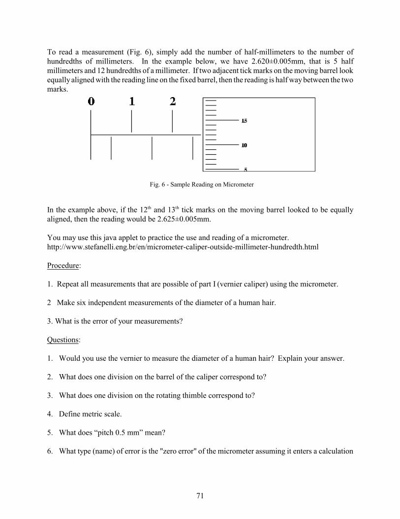
Fig. 6 - Sample Reading on Micrometer

To read a measurement (Fig. 6), simply add the number of half-millimeters to the number ofhundredths of millimeters. In the example below, we have 2.620±0.005mm, that is 5 halfmillimeters and 12 hundredths of a millimeter. If two adjacent tick marks on the moving barrel lookequally aligned with the reading line on the fixed barrel, then the reading is half way between the twomarks.

In the example above, if the 12th and 13th tick marks on the moving barrel looked to be equallyaligned, then the reading would be 2.625±0.005mm.

You may use this java applet to practice the use and reading of a micrometer.http://www.stefanelli.eng.br/en/micrometer-caliper-outside-millimeter-hundredth.html

Procedure:

1. Repeat all measurements that are possible of part I (vernier caliper) using the micrometer.

2 Make six independent measurements of the diameter of a human hair.

3. What is the error of your measurements?

Questions:

1. Would you use the vernier to measure the diameter of a human hair? Explain your answer.

2. What does one division on the barrel of the caliper correspond to?

3. What does one division on the rotating thimble correspond to?

4. Define metric scale.

5. What does “pitch 0.5 mm” mean?

6. What type (name) of error is the "zero error" of the micrometer assuming it enters a calculation

71

72

73

EQUILIBRIUM OF A RIGID BODY Apparatus

:

- Meter stick - One knife-edge meter stick clamp without clips - Two knife-edge meter stick clamps with clips - Two 50gr hangers - Slotted weights - Meter stick support stand - Large friction box - Electronic balance Introduction

:

If a rigid body is in equilibrium, then the vector sum of the external forces acting on the body yields a zero resultant and the sum of the torques of the external forces about any arbitrary axis is also equal to zero. Stated in equation form:

𝛴𝐹 = 0 𝛴𝜏 = 0 𝐸𝑞. 1 In this lab work force is defined as the mass m times gravitational acceleration g:

𝐹 = 𝑚𝑔 𝐸𝑞. 2 where m is in kg and g in m/s2 therefore, force F is in newtons N. Torque is a measure of how effective a given force is at twisting or turning the object it is applied to. Torque is defined as the force F times the moment arm or lever arm r of the force with respect to a selected pivot point x. In other words r is the distance from the pivot to the point where a force is applied. If the force is perpendicular to r, then

𝜏 = 𝐹𝑟 𝐸𝑞. 3 The unit of torque is Newton-meter, N∙m. The sign for torque is defined as positive (+) when rotating in counter-clockwise direction and negative (-) when rotating in a clockwise direction. In this experiment a meter stick is used as a rigid body to illustrate the application of the equations of equilibrium. The torque equation will be verified for a balanced system of two masses. The torque equation will also be applied to determine the mass of the meter stick and compare to the known value. For this experiment it is not only important to familiarize yourself with the equations, but also with sketching free-body diagrams (FBD). Next are examples of balanced systems and application of the torque equation. The equations must be solved as a pre-lab exercise.

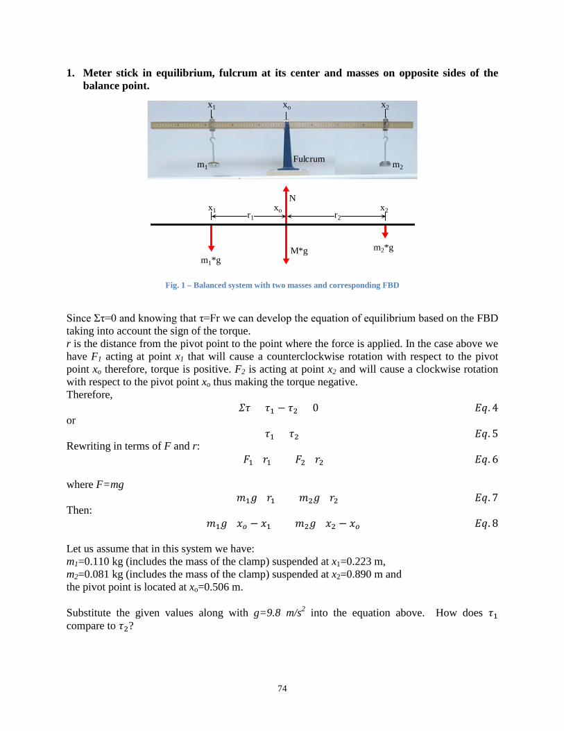
74

1. Meter stick in equilibrium, fulcrum at its center and masses on opposite sides of the balance point.

Fig. 1 – Balanced system with two masses and corresponding FBD

Since Στ=0 and knowing that τ=Fr we can develop the equation of equilibrium based on the FBD taking into account the sign of the torque. r is the distance from the pivot point to the point where the force is applied. In the case above we have F1 acting at point x1 that will cause a counterclockwise rotation with respect to the pivot point xo therefore, torque is positive. F2 is acting at point x2 and will cause a clockwise rotation with respect to the pivot point xo thus making the torque negative. Therefore,

𝛴𝜏 = 𝜏1 − 𝜏2 = 0 𝐸𝑞. 4 or

𝜏1 = 𝜏2 𝐸𝑞. 5 Rewriting in terms of F and r:

(𝐹1)(𝑟1) = (𝐹2)(𝑟2) 𝐸𝑞. 6 where F=mg

(𝑚1𝑔)(𝑟1) = (𝑚2𝑔)(𝑟2) 𝐸𝑞. 7 Then:

(𝑚1𝑔)(𝑥𝑜 − 𝑥1) = (𝑚2𝑔)(𝑥2 − 𝑥𝑜) 𝐸𝑞. 8 Let us assume that in this system we have: m1=0.110 kg (includes the mass of the clamp) suspended at x1=0.223 m, m2=0.081 kg (includes the mass of the clamp) suspended at x2=0.890 m and the pivot point is located at xo=0.506 m. Substitute the given values along with g=9.8 m/s2 into the equation above. How does 𝜏1 compare to 𝜏2?

Fulcrum

x1 xo x2

m1 m2

x1 xo x2

m1*g

r1 r2

N

M*g m2*g

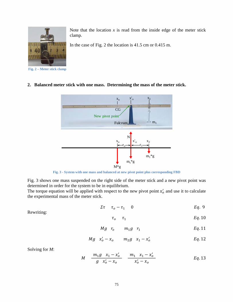
75

Note that the location x is read from the inside edge of the meter stick clamp. In the case of Fig. 2 the location is 41.5 cm or 0.415 m.

2. Balanced meter stick with one mass. Determining the mass of the meter stick.

Fulcrum

x'o

m1

xo x1

CG

xo x'o x2

m1*g

ro r1

N

M*gms*g

New pivot point

Fig. 3 - System with one mass and balanced at new pivot point plus corresponding FBD

Fig. 3 shows one mass suspended on the right side of the meter stick and a new pivot point was determined in order for the system to be in equilibrium. The torque equation will be applied with respect to the new pivot point 𝑥𝑜′ and use it to calculate the experimental mass of the meter stick.

𝛴𝜏 = 𝜏𝑜 − 𝜏1 = 0 𝐸𝑞. 9 Rewriting:

𝜏𝑜 = 𝜏1 𝐸𝑞. 10

(𝑀𝑔)(𝑟𝑜) = (𝑚1𝑔)(𝑟1) 𝐸𝑞. 11

(𝑀𝑔)(𝑥𝑜′ − 𝑥𝑜) = (𝑚2𝑔)(𝑥1 − 𝑥𝑜′ ) 𝐸𝑞. 12 Solving for M:

𝑀 =(𝑚1𝑔)(𝑥1 − 𝑥𝑜′ )

(𝑔)(𝑥𝑜′ − 𝑥𝑜)=

(𝑚1)(𝑥1 − 𝑥𝑜′ )(𝑥𝑜′ − 𝑥𝑜)

𝐸𝑞. 13

Fig. 2 – Meter stick clamp

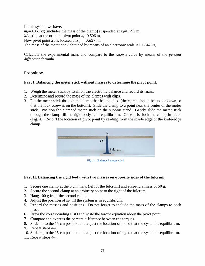
76

In this system we have: m1=0.061 kg (includes the mass of the clamp) suspended at x1=0.792 m, M acting at the original pivot point xo=0.506 m, New pivot point 𝑥𝑜′ is located at 𝑥𝑜′ = 0.627 m. The mass of the meter stick obtained by means of an electronic scale is 0.0842 kg. Calculate the experimental mass and compare to the known value by means of the percent difference formula. Procedure

:

Part I. Balancing the meter stick without masses to determine the pivot point

:

1. Weigh the meter stick by itself on the electronic balance and record its mass. 2. Determine and record the mass of the clamps with clips. 3. Put the meter stick through the clamp that has no clips (the clamp should be upside down so

that the lock screw is on the bottom). Slide the clamp to a point near the center of the meter stick. Position the clamped meter stick on the support stand. Gently slide the meter stick through the clamp till the rigid body is in equilibrium. Once it is, lock the clamp in place (Fig. 4). Record the location of pivot point by reading from the inside edge of the knife-edge clamp.

Fulcrum

xo

CG

Fig. 4 – Balanced meter stick

Part II. Balancing the rigid body with two masses on opposite sides of the fulcrum

:

1. Secure one clamp at the 5 cm mark (left of the fulcrum) and suspend a mass of 50 g. 2. Secure the second clamp at an arbitrary point to the right of the fulcrum. 3. Hang 100 g from the second clamp. 4. Adjust the position of m2 till the system is in equilibrium. 5. Record the masses and positions. Do not forget to include the mass of the clamps to each

mass. 6. Draw the corresponding FBD and write the torque equation about the pivot point. 7. Compare and express the percent difference between the torques. 8. Slide m1 to the 15 cm position and adjust the location of m2 so that the system is equilibrium. 9. Repeat steps 4-7. 10. Slide m1 to the 25 cm position and adjust the location of m2 so that the system is equilibrium. 11. Repeat steps 4-7.

77

Part III. Obtaining the mass of the meter stick by method of torques

:

1. Balance the meter stick by itself. 2. Position one clamp at the 5 cm mark and suspend 100 g from it. 3. Find a new pivot point that will bring the system to equilibrium. Record the location. 4. Using the torque equation calculate the mass of the meter stick. 5. Compare the obtained value with the value you found when weighing the meter stick.

Questions

:

1. A meter stick is balanced at its center. If a 3 kg mass is suspended at x=0 m, where would you need to place a mass of 5 kg to have the system in equilibrium?

2. What will happen if the meter stick is not strictly horizontal? 3. Can we apply the torque balance equation if the stick is not horizontal? What must be

changed in Eq. 3, 6, 7, 8, 11, 12 and 13 in this case?

78

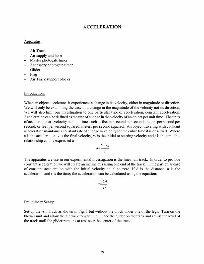
ACCELERATION

Apparatus:

S Air TrackS Air supply and hoseS Master photogate timerS Accessory photogate timerS GliderS FlagS Air Track support blocks

Introduction:

When an object accelerates it experiences a change in its velocity, either in magnitude or direction. We will only be examining the case of a change in the magnitude of the velocity not its direction. We will also limit our investigation to one particular type of acceleration, constant acceleration. Acceleration can be defined as the rate of change in the velocity of an object per unit time. The unitsof acceleration are velocity per unit time, such as feet per second per second, meters per second persecond, or feet per second squared, meters per second squared. An object traveling with constantacceleration maintains a constant rate of change in velocity for the entire time it is observed. Wherea is the acceleration, v is the final velocity, v0 is the initial or starting velocity and t is the time thisrelationship can be expressed as:

The apparatus we use in our experimental investigation is the linear air track. In order to provideconstant acceleration we will create an incline by raising one end of the track. In the particular caseof constant acceleration with the initial velocity equal to zero, if d is the distance, a is theacceleration and t is the time; the acceleration can be calculated using the equation:

Preliminary Set-up:

Set-up the Air Track as shown in Fig. 1 but without the block under one of the legs. Turn on theblower unit and allow the air track to warm up. Place the glider on the track and adjust the level ofthe track until the glider remains at rest near the center of the track.

79

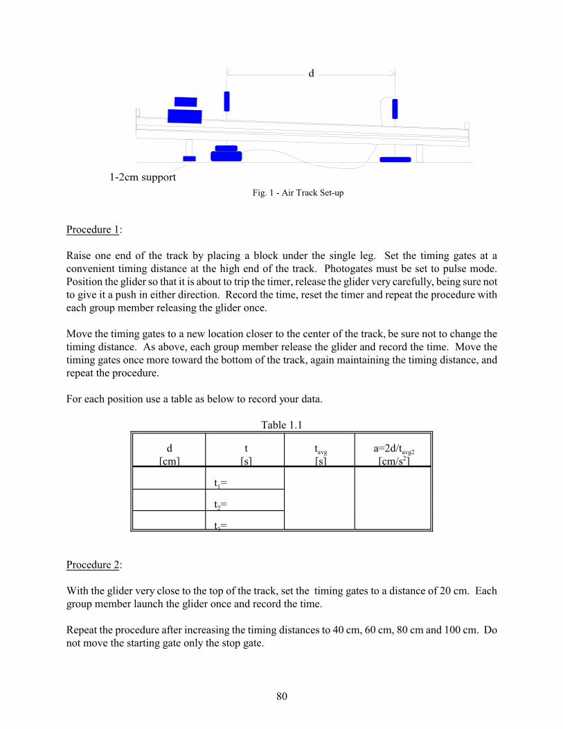
Fig. 1 - Air Track Set-up

Procedure 1:

Raise one end of the track by placing a block under the single leg. Set the timing gates at aconvenient timing distance at the high end of the track. Photogates must be set to pulse mode. Position the glider so that it is about to trip the timer, release the glider very carefully, being sure notto give it a push in either direction. Record the time, reset the timer and repeat the procedure witheach group member releasing the glider once.

Move the timing gates to a new location closer to the center of the track, be sure not to change thetiming distance. As above, each group member release the glider and record the time. Move thetiming gates once more toward the bottom of the track, again maintaining the timing distance, andrepeat the procedure.

For each position use a table as below to record your data.

Table 1.1

d[cm]

t[s]

tavg

[s]a=2d/tavg2

[cm/s2]

t1=

t2=

t3=

Procedure 2:

With the glider very close to the top of the track, set the timing gates to a distance of 20 cm. Eachgroup member launch the glider once and record the time.

Repeat the procedure after increasing the timing distances to 40 cm, 60 cm, 80 cm and 100 cm. Donot move the starting gate only the stop gate.

80

Table 2.1

d[cm]

t[s]

tavg

[s]tavg2

[s2]a=2d/tavg2

[cm/s2]

20

t1=

t2=

t3=

40

t1=

t2=

t3=

60

t1=

t2=

t3=

80

t1=

t2=

t3=

100

t1=

t2=

t3=

Calculations:

1. For each step in each procedure calculate the average time.

2. For Procedure 2 use the second equation, the distance and the average time squared to calculatethe average acceleration for each position. Compare these accelerations, are they equal? Howmuch do you trust your results? Discuss the answers in your conclusion.

Graphs:

1. Plot a graph of d vs. tavg

2. Plot a graph of d vs tavg2

Discuss these graphs in your conclusion. Use the slope of the second graph to find the acceleration,how does this acceleration compare to the average acceleration from Procedure 1?

81

82

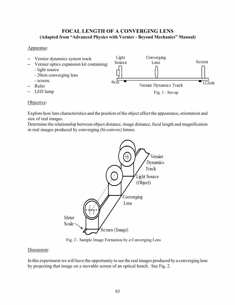
FOCAL LENGTH OF A CONVERGING LENS(Adapted from “Advanced Physics with Vernier - Beyond Mechanics” Manual)

Apparatus:

S Vernier dynamics system trackS Vernier optics expansion kit containing:

- light source- 20cm converging lens

- screen.S RulerS LED lamp

Objective:

Explore how lens characteristics and the position of the object affect the appearance, orientation andsize of real images. Determine the relationship between object distance, image distance, focal length and magnificationin real images produced by converging (bi-convex) lenses.

Discussion:

In this experiment we will have the opportunity to see the real images produced by a converging lensby projecting that image on a movable screen of an optical bench. See Fig. 2.

Fig. 1 - Set-up

Fig. 2 - Sample Image Formation by a Converging Lens

83

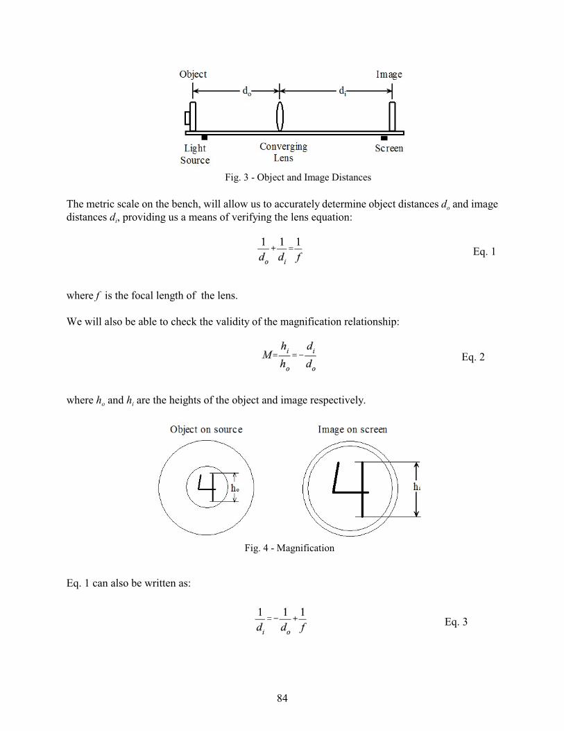
Eq. 1

Eq. 2

Eq. 3

The metric scale on the bench, will allow us to accurately determine object distances do and imagedistances di, providing us a means of verifying the lens equation:

where f is the focal length of the lens.

We will also be able to check the validity of the magnification relationship:

where ho and hi are the heights of the object and image respectively.

Eq. 1 can also be written as:

Fig. 3 - Object and Image Distances

Fig. 4 - Magnification

84

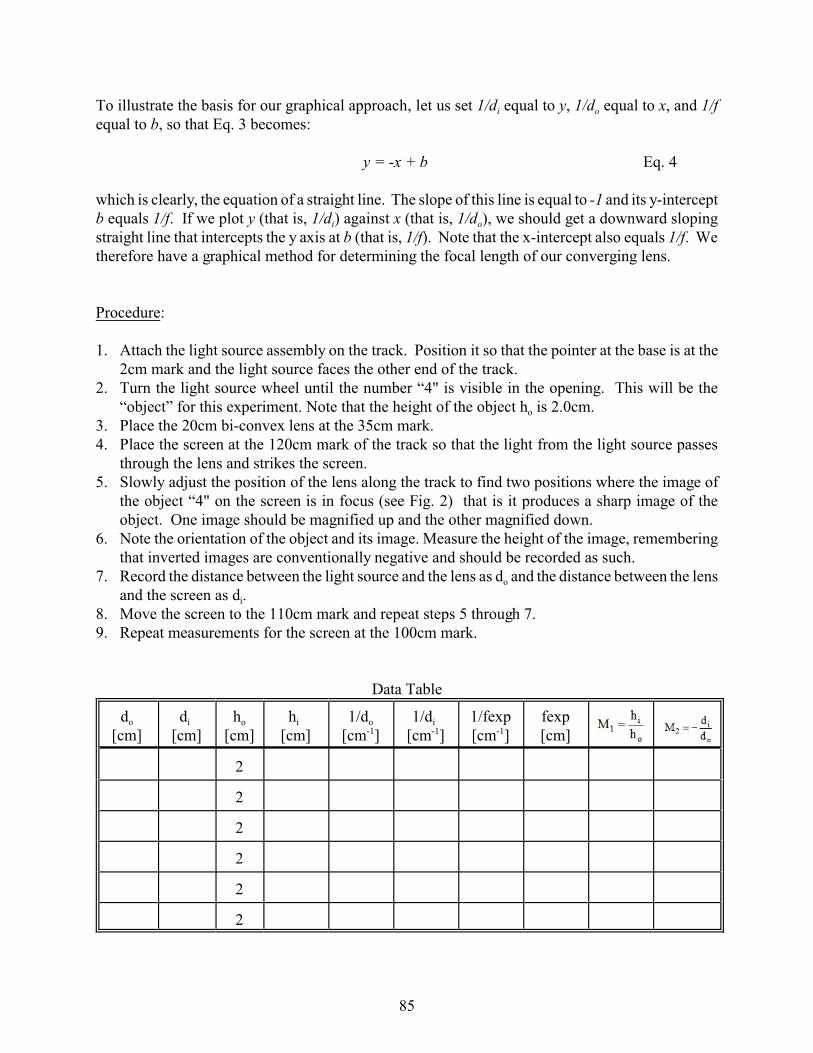
To illustrate the basis for our graphical approach, let us set 1/di equal to y, 1/do equal to x, and 1/fequal to b, so that Eq. 3 becomes:

y = -x + b Eq. 4

which is clearly, the equation of a straight line. The slope of this line is equal to -1 and its y-interceptb equals 1/f. If we plot y (that is, 1/di) against x (that is, 1/do), we should get a downward slopingstraight line that intercepts the y axis at b (that is, 1/f). Note that the x-intercept also equals 1/f. Wetherefore have a graphical method for determining the focal length of our converging lens.

Procedure:

1. Attach the light source assembly on the track. Position it so that the pointer at the base is at the2cm mark and the light source faces the other end of the track.

2. Turn the light source wheel until the number “4" is visible in the opening. This will be the“object” for this experiment. Note that the height of the object ho is 2.0cm.

3. Place the 20cm bi-convex lens at the 35cm mark. 4. Place the screen at the 120cm mark of the track so that the light from the light source passes

through the lens and strikes the screen. 5. Slowly adjust the position of the lens along the track to find two positions where the image of

the object “4" on the screen is in focus (see Fig. 2) that is it produces a sharp image of theobject. One image should be magnified up and the other magnified down.

6. Note the orientation of the object and its image. Measure the height of the image, rememberingthat inverted images are conventionally negative and should be recorded as such.

7. Record the distance between the light source and the lens as do and the distance between the lensand the screen as di.

8. Move the screen to the 110cm mark and repeat steps 5 through 7. 9. Repeat measurements for the screen at the 100cm mark.

Data Table

do

[cm]di

[cm]ho

[cm]hi

[cm]1/do

[cm-1]1/di

[cm-1]1/fexp[cm-1]

fexp[cm]

2

2

2

2

2

2

85

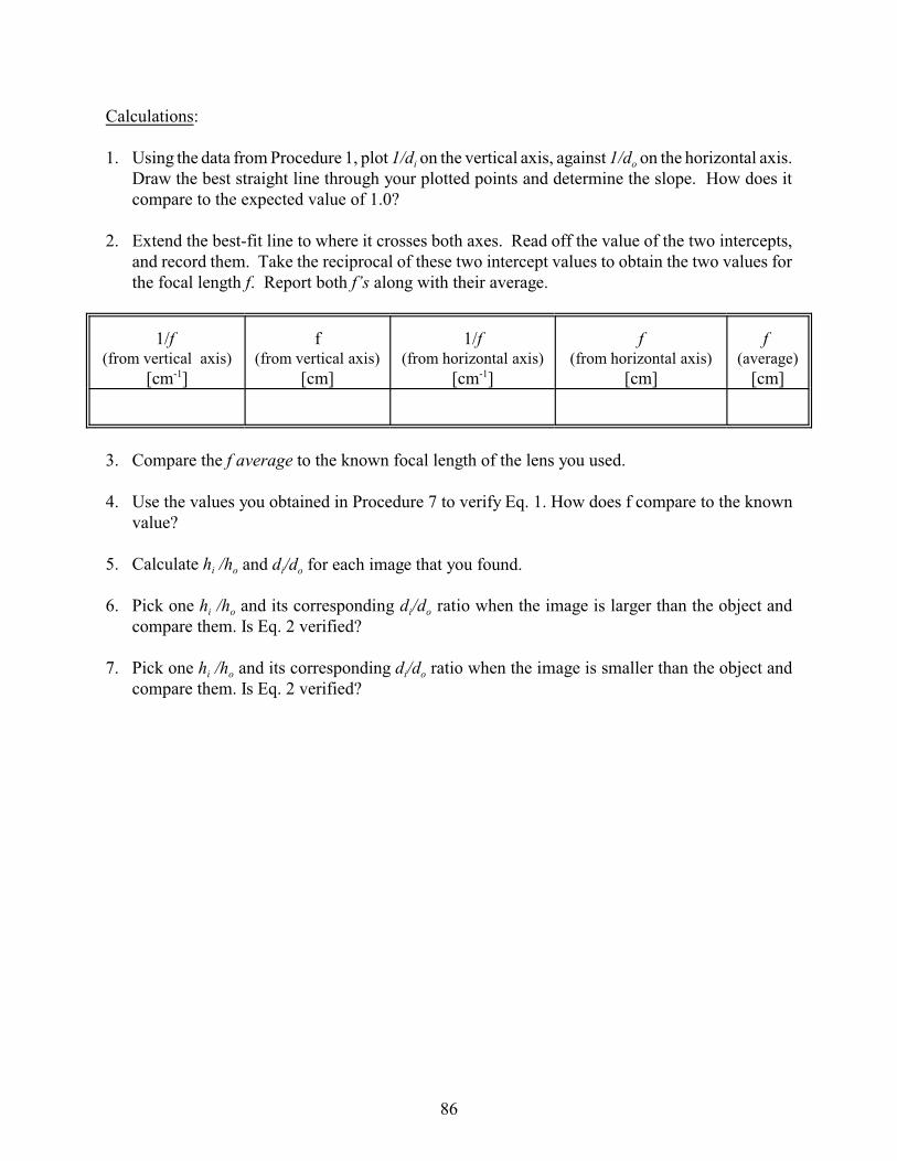
Calculations:

1. Using the data from Procedure 1, plot 1/di on the vertical axis, against 1/do on the horizontal axis. Draw the best straight line through your plotted points and determine the slope. How does itcompare to the expected value of 1.0?

2. Extend the best-fit line to where it crosses both axes. Read off the value of the two intercepts,and record them. Take the reciprocal of these two intercept values to obtain the two values forthe focal length f. Report both f’s along with their average.

1/f (from vertical axis)

[cm-1]

f(from vertical axis)

[cm]

1/f(from horizontal axis)

[cm-1]

f(from horizontal axis)

[cm]

f (average)

[cm]

3. Compare the f average to the known focal length of the lens you used.

4. Use the values you obtained in Procedure 7 to verify Eq. 1. How does f compare to the knownvalue?

5. Calculate hi /ho and di/do for each image that you found.

6. Pick one hi /ho and its corresponding di/do ratio when the image is larger than the object andcompare them. Is Eq. 2 verified?

7. Pick one hi /ho and its corresponding di/do ratio when the image is smaller than the object andcompare them. Is Eq. 2 verified?

86

APPENDIX

87

88

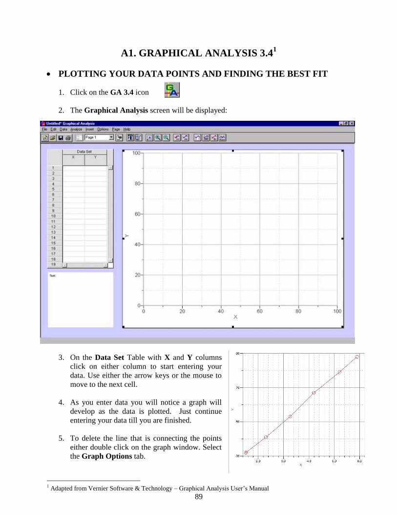
89

A1. GRAPHICAL ANALYSIS 3.41

PLOTTING YOUR DATA POINTS AND FINDING THE BEST FIT

1. Click on the GA 3.4 icon

2. The Graphical Analysis screen will be displayed:

3. On the Data Set Table with X and Y columns

click on either column to start entering your

data. Use either the arrow keys or the mouse to

move to the next cell.

4. As you enter data you will notice a graph will

develop as the data is plotted. Just continue

entering your data till you are finished.

5. To delete the line that is connecting the points

either double click on the graph window. Select

the Graph Options tab.

1 Adapted from Vernier Software & Technology – Graphical Analysis User’s Manual

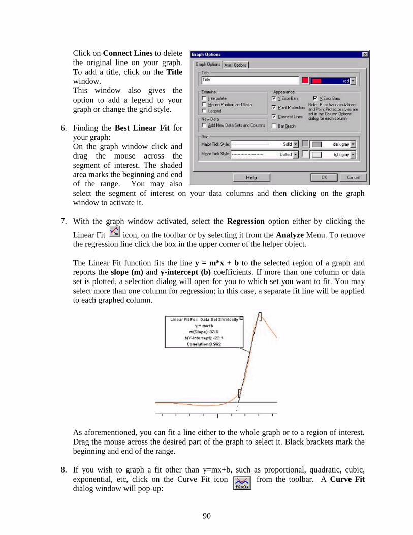
90

Click on Connect Lines to delete

the original line on your graph.

To add a title, click on the Title

window.

This window also gives the

option to add a legend to your

graph or change the grid style.

6. Finding the Best Linear Fit for

your graph:

On the graph window click and

drag the mouse across the

segment of interest. The shaded

area marks the beginning and end

of the range. You may also

select the segment of interest on your data columns and then clicking on the graph

window to activate it.

7. With the graph window activated, select the Regression option either by clicking the

Linear Fit icon, on the toolbar or by selecting it from the Analyze Menu. To remove

the regression line click the box in the upper corner of the helper object.

The Linear Fit function fits the line y = m*x + b to the selected region of a graph and

reports the slope (m) and y-intercept (b) coefficients. If more than one column or data

set is plotted, a selection dialog will open for you to which set you want to fit. You may

select more than one column for regression; in this case, a separate fit line will be applied

to each graphed column.

As aforementioned, you can fit a line either to the whole graph or to a region of interest.

Drag the mouse across the desired part of the graph to select it. Black brackets mark the

beginning and end of the range.

8. If you wish to graph a fit other than y=mx+b, such as proportional, quadratic, cubic,

exponential, etc, click on the Curve Fit icon from the toolbar. A Curve Fit

dialog window will pop-up:

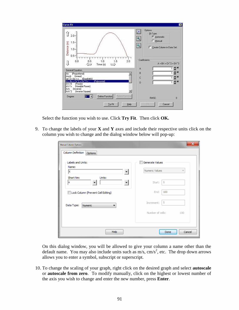
91

Select the function you wish to use. Click Try Fit. Then click OK.

9. To change the labels of your X and Y axes and include their respective units click on the

column you wish to change and the dialog window below will pop-up:

On this dialog window, you will be allowed to give your column a name other than the

default name. You may also include units such as m/s, cm/s2, etc. The drop down arrows

allows you to enter a symbol, subscript or superscript.

10. To change the scaling of your graph, right click on the desired graph and select autoscale

or autoscale from zero. To modify manually, click on the highest or lowest number of

the axis you wish to change and enter the new number, press Enter.

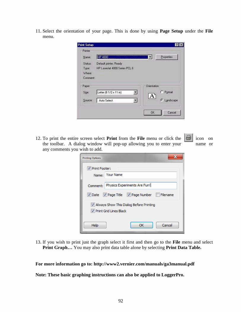
92

11. Select the orientation of your page. This is done by using Page Setup under the File

menu.

12. To print the entire screen select Print from the File menu or click the icon on

the toolbar. A dialog window will pop-up allowing you to enter your name or

any comments you wish to add.

13. If you wish to print just the graph select it first and then go to the File menu and select

Print Graph… You may also print data table alone by selecting Print Data Table.

For more information go to: http://www2.vernier.com/manuals/ga3manual.pdf

Note: These basic graphing instructions can also be applied to LoggerPro.

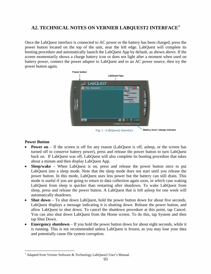
93

A2. TECHNICAL NOTES ON VERNIER LABQUEST2 INTERFACE1

Once the LabQuest interface is connected to AC power or the battery has been charged, press the power button located on the top of the unit, near the left edge. LabQuest will complete its booting procedure and automatically launch the LabQuest App by default, as shown above. If the screen momentarily shows a charge battery icon or does not light after a moment when used on battery power, connect the power adapter to LabQuest and to an AC power source, then try the power button again.

Power Button • Power on – If the screen is off for any reason (LabQuest is off, asleep, or the screen has

turned off to conserve battery power), press and release the power button to turn LabQuest back on. If LabQuest was off, LabQuest will also complete its booting procedure that takes about a minute and then display LabQuest App.

• Sleep/wake – When LabQuest is on, press and release the power button once to put LabQuest into a sleep mode. Note that the sleep mode does not start until you release the power button. In this mode, LabQuest uses less power but the battery can still drain. This mode is useful if you are going to return to data collection again soon, in which case waking LabQuest from sleep is quicker than restarting after shutdown. To wake LabQuest from sleep, press and release the power button. A LabQuest that is left asleep for one week will automatically shutdown.

• Shut down – To shut down LabQuest, hold the power button down for about five seconds. LabQuest displays a message indicating it is shutting down. Release the power button, and allow LabQuest to shut down. To cancel the shutdown procedure at this point, tap Cancel. You can also shut down LabQuest from the Home screen. To do this, tap System and then tap Shut Down.

• Emergency shutdown – If you hold the power button down for about eight seconds, while it is running. This is not recommended unless LabQuest is frozen, as you may lose your data and potentially cause file system corruption.

1 Adapted from Vernier Software & Technology LabQuest2 User’s Manual.

Fig. 1 - LabQuest2 Interface

94

Touch Screen LabQuest has an LED backlit resistive touch screen that quickly responds to pressure exerted on the screen. LabQuest is controlled primarily by touching the screen. The software is designed to be finger-friendly. In some situations, you may desire more control for precise navigation. In such cases, we recommend using the included stylus. If you are having trouble viewing the color screen or are using LabQuest outside in bright sunlight, we recommend changing to the High Contrast mode. Tap Preferences on the Home screen, then tap Light & Power. Select the check box for High Contrast to enable this mode. Hardware Keys In addition to using the touch screen, the three hardware keys can also be used to control your LabQuest. • Collect – Start and stop data collection within LabQuest App • Home – Launch the Home screen to access other applications • Escape – Close most applications, menus, and exit dialog boxes without taking action (i.e.,

cancel dialog boxes)

Sensor Ports LabQuest has three analog sensor ports (CH 1, CH 2, and CH 3) for analog sensors such as our pH Sensor, Temperature Probe, and Force Sensor. Also included is a full-size USB port for USB sensors, USB flash drives, and USB printers. In addition to the power button, the top edge of LabQuest has two digital sensor ports (DIG 1 and DIG 2) for Motion Detectors, Drop Counters, and other digital sensors.

Fig. 2 - LabQuest2 Control Buttons

Fig. 3- LabQuest2 Sensor Ports

95

Audio ports are also located adjacent to the digital ports, as well as a microSD card slot for expanding disk storage. On the side opposite of the analog ports, there is a stylus storage slot, an AC power port for recharging the battery, and a mini USB port for connecting LabQuest to a computer. In between these ports, there is a serial connection for charging the unit in a LabQuest Charging Station.

For more information on the LabQuest2 interface please go to: http://www2.vernier.com/manuals/labquest2_user_manual.pdf

Fig. 4 - LabQuest2 Additional Ports

96

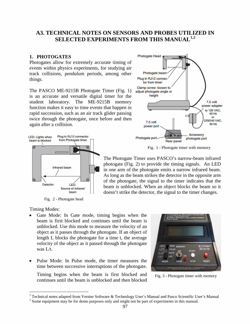
97

A3. TECHNICAL NOTES ON SENSORS AND PROBES UTILIZED IN SELECTED EXPERIMENTS FROM THIS MANUAL1,2

1. PHOTOGATES Photogates allow for extremely accurate timing of events within physics experiments, for studying air track collisions, pendulum periods, among other things. The PASCO ME-9215B Photogate Timer (Fig. 1) is an accurate and versatile digital timer for the student laboratory. The ME-9215B memory function makes it easy to time events that happen in rapid succession, such as an air track glider passing twice through the photogate, once before and then again after a collision.

The Photogate Timer uses PASCO’s narrow-beam infrared photogate (Fig. 2) to provide the timing signals. An LED in one arm of the photogate emits a narrow infrared beam. As long as the beam strikes the detector in the opposite arm of the photogate, the signal to the timer indicates that the beam is unblocked. When an object blocks the beam so it doesn’t strike the detector, the signal to the timer changes.

Timing Modes: • Gate Mode: In Gate mode, timing begins when the

beam is first blocked and continues until the beam is unblocked. Use this mode to measure the velocity of an object as it passes through the photogate. If an object of length L blocks the photogate for a time t, the average velocity of the object as it passed through the photogate was L/t.

• Pulse Mode: In Pulse mode, the timer measures the

time between successive interruptions of the photogate.

Timing begins when the beam is first blocked and continues until the beam is unblocked and then blocked

1 Technical notes adapted from Vernier Software & Technology User’s Manual and Pasco Scientific User’s Manual 2 Some equipment may be for demo purposes only and might not be part of experiments in this manual.

Fig. 3 - Photogate timer with memory

Fig. 1 - Photogate timer with memory

Fig. 2 - Photogate head

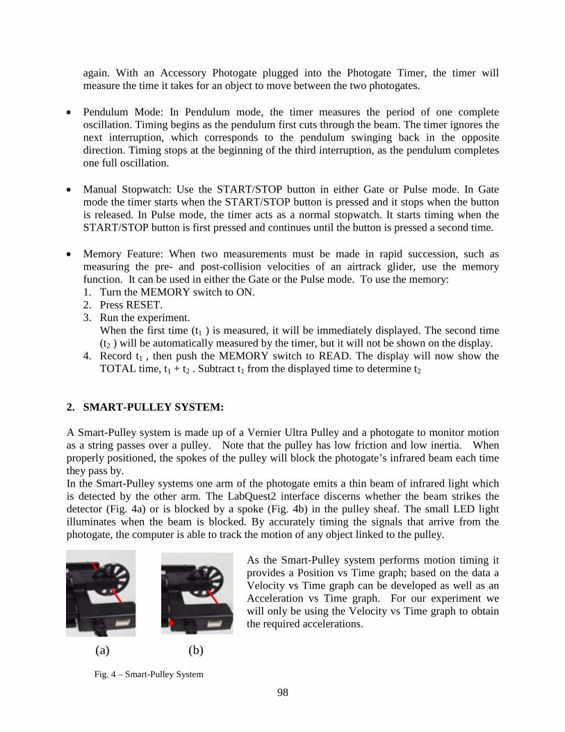
98

again. With an Accessory Photogate plugged into the Photogate Timer, the timer will measure the time it takes for an object to move between the two photogates.

• Pendulum Mode: In Pendulum mode, the timer measures the period of one complete

oscillation. Timing begins as the pendulum first cuts through the beam. The timer ignores the next interruption, which corresponds to the pendulum swinging back in the opposite direction. Timing stops at the beginning of the third interruption, as the pendulum completes one full oscillation.

• Manual Stopwatch: Use the START/STOP button in either Gate or Pulse mode. In Gate

mode the timer starts when the START/STOP button is pressed and it stops when the button is released. In Pulse mode, the timer acts as a normal stopwatch. It starts timing when the START/STOP button is first pressed and continues until the button is pressed a second time.

• Memory Feature: When two measurements must be made in rapid succession, such as

measuring the pre- and post-collision velocities of an airtrack glider, use the memory function. It can be used in either the Gate or the Pulse mode. To use the memory: 1. Turn the MEMORY switch to ON. 2. Press RESET. 3. Run the experiment.

When the first time (t1 ) is measured, it will be immediately displayed. The second time (t2 ) will be automatically measured by the timer, but it will not be shown on the display.

4. Record t1 , then push the MEMORY switch to READ. The display will now show the TOTAL time, t1 + t2 . Subtract t1 from the displayed time to determine t2

2. SMART-PULLEY SYSTEM: A Smart-Pulley system is made up of a Vernier Ultra Pulley and a photogate to monitor motion as a string passes over a pulley. Note that the pulley has low friction and low inertia. When properly positioned, the spokes of the pulley will block the photogate’s infrared beam each time they pass by. In the Smart-Pulley systems one arm of the photogate emits a thin beam of infrared light which is detected by the other arm. The LabQuest2 interface discerns whether the beam strikes the detector (Fig. 4a) or is blocked by a spoke (Fig. 4b) in the pulley sheaf. The small LED light illuminates when the beam is blocked. By accurately timing the signals that arrive from the photogate, the computer is able to track the motion of any object linked to the pulley.

As the Smart-Pulley system performs motion timing it provides a Position vs Time graph; based on the data a Velocity vs Time graph can be developed as well as an Acceleration vs Time graph. For our experiment we will only be using the Velocity vs Time graph to obtain the required accelerations.

Fig. 4 – Smart-Pulley System

(a) (b)

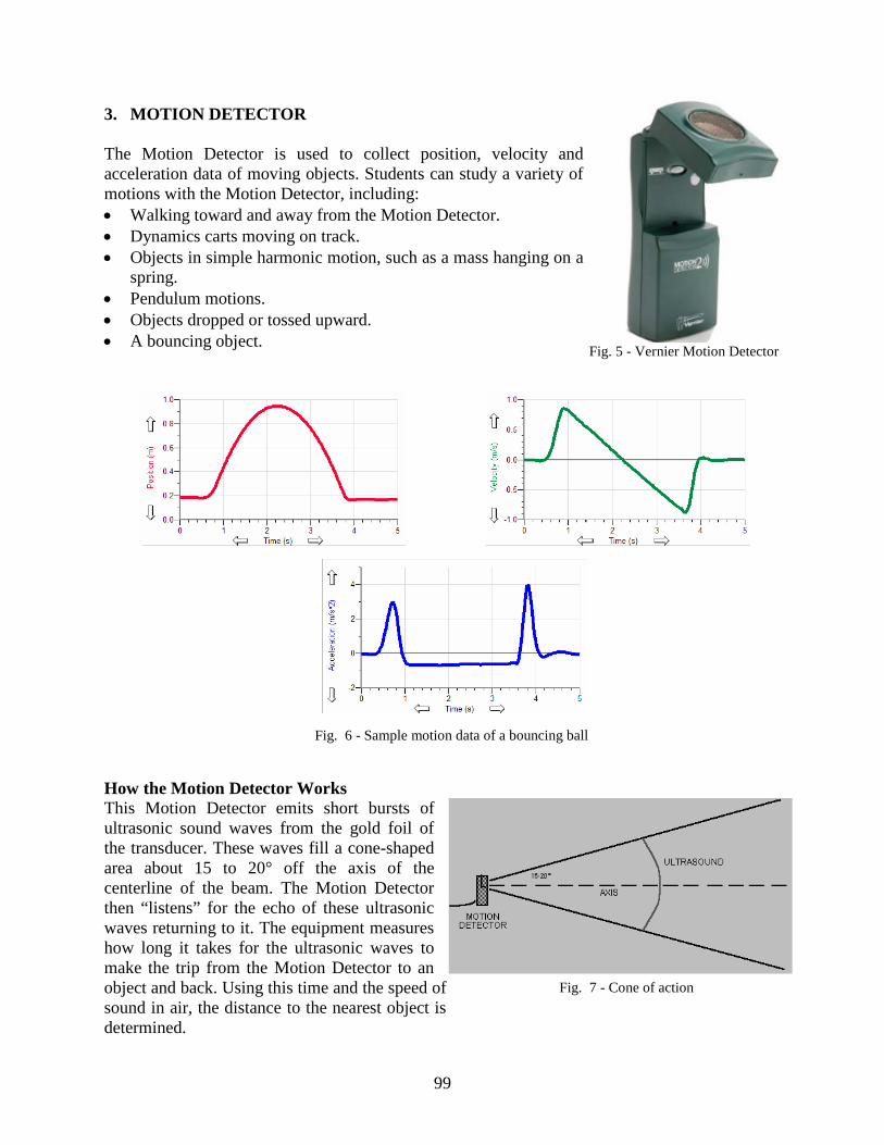
99

3. MOTION DETECTOR The Motion Detector is used to collect position, velocity and acceleration data of moving objects. Students can study a variety of motions with the Motion Detector, including: • Walking toward and away from the Motion Detector. • Dynamics carts moving on track. • Objects in simple harmonic motion, such as a mass hanging on a

spring. • Pendulum motions. • Objects dropped or tossed upward. • A bouncing object.

How the Motion Detector Works This Motion Detector emits short bursts of ultrasonic sound waves from the gold foil of the transducer. These waves fill a cone-shaped area about 15 to 20° off the axis of the centerline of the beam. The Motion Detector then “listens” for the echo of these ultrasonic waves returning to it. The equipment measures how long it takes for the ultrasonic waves to make the trip from the Motion Detector to an object and back. Using this time and the speed of sound in air, the distance to the nearest object is determined.

Fig. 5 - Vernier Motion Detector

Fig. 6 - Sample motion data of a bouncing ball

Fig. 7 - Cone of action

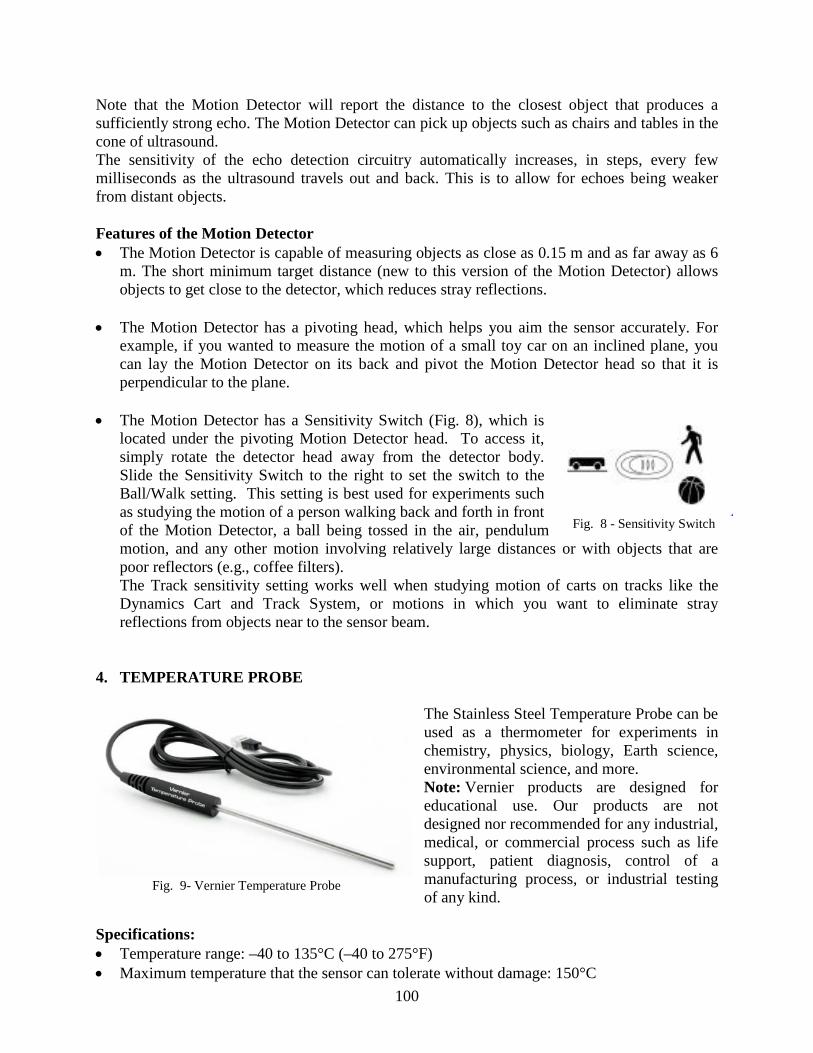
100

Note that the Motion Detector will report the distance to the closest object that produces a sufficiently strong echo. The Motion Detector can pick up objects such as chairs and tables in the cone of ultrasound. The sensitivity of the echo detection circuitry automatically increases, in steps, every few milliseconds as the ultrasound travels out and back. This is to allow for echoes being weaker from distant objects. Features of the Motion Detector • The Motion Detector is capable of measuring objects as close as 0.15 m and as far away as 6

m. The short minimum target distance (new to this version of the Motion Detector) allows objects to get close to the detector, which reduces stray reflections.

• The Motion Detector has a pivoting head, which helps you aim the sensor accurately. For example, if you wanted to measure the motion of a small toy car on an inclined plane, you can lay the Motion Detector on its back and pivot the Motion Detector head so that it is perpendicular to the plane.

• The Motion Detector has a Sensitivity Switch (Fig. 8), which is

located under the pivoting Motion Detector head. To access it, simply rotate the detector head away from the detector body. Slide the Sensitivity Switch to the right to set the switch to the Ball/Walk setting. This setting is best used for experiments such as studying the motion of a person walking back and forth in front of the Motion Detector, a ball being tossed in the air, pendulum motion, and any other motion involving relatively large distances or with objects that are poor reflectors (e.g., coffee filters). The Track sensitivity setting works well when studying motion of carts on tracks like the Dynamics Cart and Track System, or motions in which you want to eliminate stray reflections from objects near to the sensor beam.

4. TEMPERATURE PROBE

The Stainless Steel Temperature Probe can be used as a thermometer for experiments in chemistry, physics, biology, Earth science, environmental science, and more. Note: Vernier products are designed for educational use. Our products are not designed nor recommended for any industrial, medical, or commercial process such as life support, patient diagnosis, control of a manufacturing process, or industrial testing of any kind.

Specifications: • Temperature range: –40 to 135°C (–40 to 275°F) • Maximum temperature that the sensor can tolerate without damage: 150°C

Fig. 8 - Sensitivity Switch

Fig. 9- Vernier Temperature Probe

101

• Typical Resolution: o .17°C (–40 to 0°C) o .03°C (0 to 40°C) o .1°C (40 to 100°C) o .25°C (100 to 135°C)

• Temperature sensor: 20 kΩ NTC Thermistor • Accuracy: ±0.2°C at 0°C, ±0.5°C at 100°C • Response time (time for 90% change in reading):

o 10 seconds (in water, with stirring) o 400 seconds (in still air) o seconds (in moving air)

• Probe dimensions: o Probe length (handle plus body): 15.5 cm o Stainless steel body: length 10.5 cm, diameter 4.0 mm o Probe handle: length 5.0 cm, diameter 1.25 cm

102

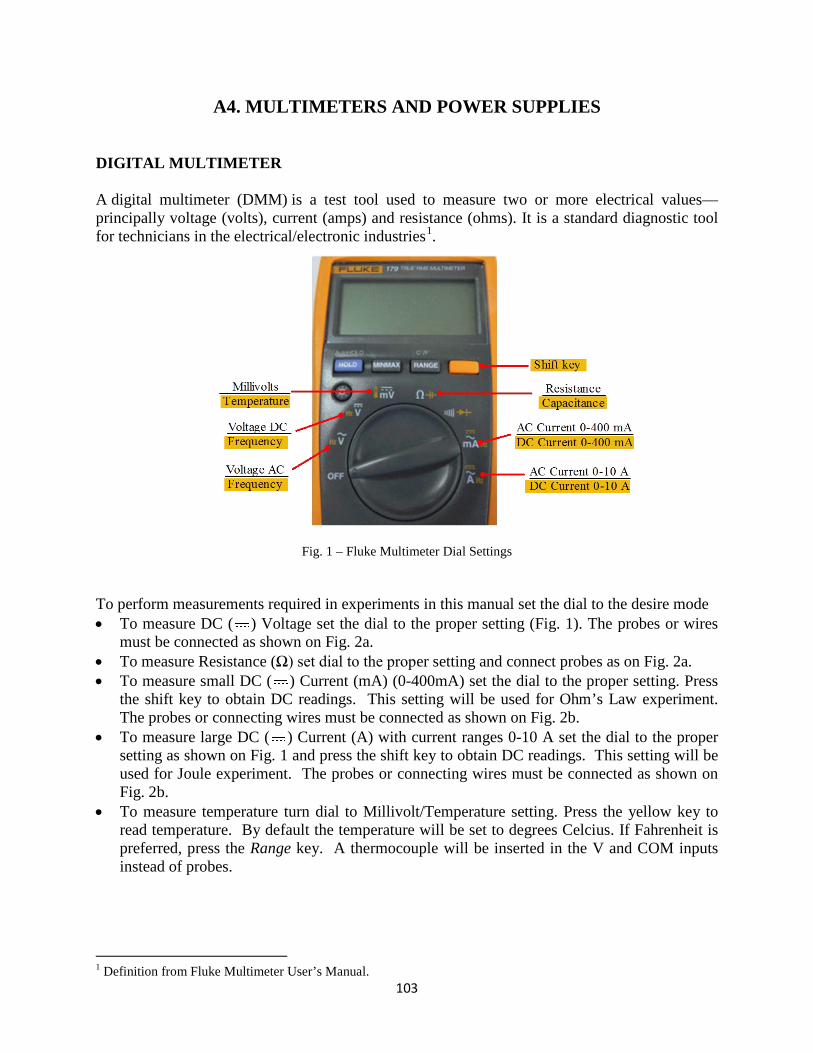
103

A4. MULTIMETERS AND POWER SUPPLIES DIGITAL MULTIMETER A digital multimeter (DMM) is a test tool used to measure two or more electrical values—principally voltage (volts), current (amps) and resistance (ohms). It is a standard diagnostic tool for technicians in the electrical/electronic industries1

.

Fig. 1 – Fluke Multimeter Dial Settings To perform measurements required in experiments in this manual set the dial to the desire mode • To measure DC ( ) Voltage set the dial to the proper setting (Fig. 1). The probes or wires

must be connected as shown on Fig. 2a. • To measure Resistance (Ω) set dial to the proper setting and connect probes as on Fig. 2a. • To measure small DC ( ) Current (mA) (0-400mA) set the dial to the proper setting. Press

the shift key to obtain DC readings. This setting will be used for Ohm’s Law experiment. The probes or connecting wires must be connected as shown on Fig. 2b.

• To measure large DC ( ) Current (A) with current ranges 0-10 A set the dial to the proper setting as shown on Fig. 1 and press the shift key to obtain DC readings. This setting will be used for Joule experiment. The probes or connecting wires must be connected as shown on Fig. 2b.

• To measure temperature turn dial to Millivolt/Temperature setting. Press the yellow key to read temperature. By default the temperature will be set to degrees Celcius. If Fahrenheit is preferred, press the Range key. A thermocouple will be inserted in the V and COM inputs instead of probes.

1 Definition from Fluke Multimeter User’s Manual.

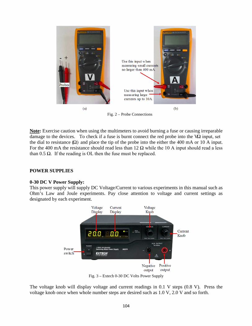
104

Fig. 2 – Probe Connections Note

: Exercise caution when using the multimeters to avoid burning a fuse or causing irreparable damage to the devices. To check if a fuse is burnt connect the red probe into the V Ω input, set the dial to resistance (Ω) and place the tip of the probe into the either the 400 mA or 10 A input. For the 400 mA the resistance should read less than 12 Ω while the 10 A input should read a less than 0.5 Ω. If the reading is OL then the fuse must be replaced.

POWER SUPPLIES 0-30 DC V Power Supply: This power supply will supply DC Voltage/Current to various experiments in this manual such as Ohm’s Law and Joule experiments. Pay close attention to voltage and current settings as designated by each experiment.

Fig. 3 – Extech 0-30 DC Volts Power Supply The voltage knob will display voltage and current readings in 0.1 V steps (0.8 V). Press the voltage knob once when whole number steps are desired such as 1.0 V, 2.0 V and so forth.

105

0-12 DC V Power Supply This power supply has various small DC Voltages settings such as 3 V, 4.5 V, 6 V, 7.5 V, 9 V and 12 V.

Fig. 4 – 0 to 12 V Power Supply

106