Embed Size (px)
Citation preview
University of Cagliari
Ph. D. Course in
INDUSTRIAL ENGINEERING
XXV Cycle
Analysis and Synthesis Techniques of Nonlinear Dynamical
Systems with Applications to Diagnostic of Controlled
Thermonuclear Fusion Reactors
Fabio Pisano
Tutor: Alessandra Fanni
Advisor: Barbara Cannas
Curriculum: ING-IND/31
2011 – 2012


Dedicated to my parents


Questa Tesi può essere utilizzata, nei limiti stabiliti dalla normativa vigente sul Diritto
d’Autore (Legge 22 aprile 1941 n. 633 e succ. modificazioni e articoli da 2575 a 2583 del
Codice civile) ed esclusivamente per scopi didattici e di ricerca; è vietato qualsiasi utilizzo
per fini commerciali. In ogni caso tutti gli utilizzi devono riportare la corretta citazione delle
fonti. La traduzione, l'adattamento totale e parziale, sono riservati per tutti i Paesi. I
documenti depositati sono sottoposti alla legislazione italiana in vigore nel rispetto del
Diritto di Autore, da qualunque luogo essi siano fruiti.


9
Contents
Acknowledgements .………………………………………………………………13
Sommario …………………………………………………………………………15
List of figures ...…………………………………………………………………...17
List of tables ...…………………………………………………………………….21
Introduction ...…………………………………………………………………….23
Part I. Theory …………………………………………………………………….27
1. Nonlinear dynamical systems analysis ......................................................29
1.1. Continuous-time dynamical systems ……………………………………….29
1.2. Discrete-time dynamical systems …………………………………………...30
1.3. Affine dynamical systems …………………………………………………..31
1.4. PWL dynamical systems …………………………………………………...33
1.5. Steady-state behaviours ……………………………………………………..34
1.6. Chaotic systems ……………………………………………………………..35
1.7. Lyapunov exponents estimation for nonlinear dynamical systems analysis ..36
1.8. Algorithms for the evaluation of Lyapunov exponents ……………………..37
2. Nonlinear dynamical systems synthesis………………………………….. 39
2.1. Synchronization of chaotic systems …….…………………………………..39
3. Data analysis and statistics ………………………………………………..41
3.1. Preliminary concepts ……………………………………………………….41
3.2. Some theoretical distributions ………………………………………………44
3.3. The memorylessness property ………………………………………………44
3.4. Maximum likelihood estimation method for unknown parameters ………...47
3.5. Goodness of fit tests ………………………………………………………...47
3.6. Analysis of variance ………………………………………………………...49
3.7. Graph theory and clique detection ………………………………………….50
4. Nonlinear time series analysis …………………………………………….53
4.1. Wavelet transform …………………………………………………………..53
4.2. Denoising by thresholding of wavelet coefficients …………………………56
4.3. Auto-correlation and cross-correlation analysis ……………………………58
4.4. State reconstruction by differential algebra ………………………………...60
4.5. Identifiability ………………………………………………………………..63
4.6. State reconstruction by embedding …………………………………………63
4.7. Lyapunov exponents estimation for nonlinear time series analysis ………..63
4.8. Hurst exponent ……………………………………………………………...64

10
5. Artificial neural networks ………………………………………………...67
5.1. Components of artificial neural networks …………………………………..67
5.2. Network topologies …………………………………………………………68
5.3. The learning paradigms ……………………………………………………..69
5.4. The perceptron ……………………………………………………………...69
5.5. The back-propagation algorithm ……………………………………………70
5.6. Training and validation ……………………………………………………..72
6. Plasma physics …………………………………………………………….75
6.1. Fusion reactions …………………………………………………………….75
6.2. Magnetic confinement ……………………………………………………...75
6.3. L-mode and H-mode ………………………………………………………..77
6.4. Edge localized modes ………………………………………………………78
Part II. Applications ……………………………………………………………...81
7. A fast algorithm for Lyapunov exponents evaluation in PWL systems ..83
7.1. Description of the algorithm ………………………………………………..83
7.2. Application to PWL chaotic systems ……………………………………….84
7.3. PWL approximation of nonlinear dynamical systems for Lyapunov exponents
estimation …………………………………………………………………...87
7.4. Application to polynomial chaotic systems ………………………………...88
7.5. Conclusions …………………………………………………………………91
8. Effect of a particular coupling on the dynamic behavior of nonlinear
systems ……………………………………………………………………..93
8.1. General approach …………………………………………………………...93
8.2. Application to PWL chaotic systems ……………………………………….94
8.2.1. Numerical results …………………………………………………..97
8.2.2. Experimental results …………………………………………….....99
8.3. Application to polynomial chaotic systems ……………………………….100
8.3.1. Numerical results …………………………………………………105
8.4. Conclusions ………………………………………………………………..105
9. Identification of parameters in nonlinear dynamical systems by neural
networks …………………………………………………………………..107
9.1. General approach ………………………………………………………….107
9.2. Application to the Chua’s circuit with cubic nonlinearity ………………...107
9.3. Conclusions ………………………………………………………………..111
11
10. Denoising of time series based on wavelet decomposition and cross-
correlation between the residuals and the denoised signal ……………113
10.1. Denoising method …………………………………………………………113
10.2. Detailed description of the threshold selection criteria …………………...114
10.3. The Lorenz system as a case of study ……………………………………..117
10.4. Application to time series from JET diagnostics ………………………….120
10.5. Conclusions ………………………………………………………………..122
11. Dynamic behaviour of Type I ELMs ……………………………………123
11.1. Database construction ……………………………………………………..123
11.2. An algorithm for finding ELMs in a Dα time series ………………………124
11.3. Distribution fitting ………………………………………………………...126
11.4. Memorylessness study …………………………………………………….129
11.5. Analysis of variance ……………………………………………………….130
11.6. Grouping pulses …………………………………………………………...131
11.6.1. Grouping by input signals ………………………………………...131
11.6.2. Grouping by input signals and experiments ………………………132
11.6.2.1. Distribution fitting of clique 16 ………………………...133
11.6.2.2. Statistical analysis of clique 19 ………………………...135
11.7. Analysis of determinism of ELM time series ……………………………..136
11.8. Conclusions ……………………………………………………………….139
Conclusions ……………………………………………………………………...140
Glossary of functions ……………………………………………………………143
Bibliography …………………………………………………………………….145
List of publications related to the thesis ……………………………………….153


13
Acknowledgements
A few words to thank all the people who have been close to me in the last three years, and
have helped me to finish this work, directly and indirectly.
First of all, I’d like to thank my supervisor Alessandra Fanni, for her support and
encouragement. A special thanks goes to Barbara Cannas, who helped me a lot and guided
during these long and intense years, and provided valuable support. She’s been a necessary
condition for the development of this thesis.
Additional but not secondary thanks go to my colleagues of the Electrotechnics research
group of the Department of Electrical and Electronic Engineering of the University of
Cagliari.
Thanks to Massimiliano Grosso for his statistical support, definitely above-average.
Part of this dissertation has been completed at JET, in the Culham Science Center. Thanks to
Andrea Murari and to all the people whose collaboration has been essential for this work.
Finally I’d like to thank my parents, for their support, and my friends.


15
Sommario
Il tema principale di questa tesi è la soluzione di problemi ingegneristici legati all’analisi e
alla sintesi di sistemi dinamici non lineari. I sistemi dinamici non lineari sono di largo
interesse per ingegneri, fisici e matematici, e questo è dovuto al fatto che la maggior parte
dei sistemi fisici in natura è intrinsecamente non lineare.
La non linearità di questi sistemi ha conseguenze sulla loro evoluzione temporale, che in
certi casi può rivelarsi del tutto imprevedibile, apparentemente casuale, seppure
fondamentalmente deterministica. I sistemi caotici sono un esempio lampante di questo
comportamento. Nella maggior parte dei casi non esistono delle regole standard per l’analisi
di questi sistemi. Spesso, le soluzioni non possono essere ottenute in forma chiusa, ed è
necessario ricorrere a tecniche di integrazione numerica, che, in caso di elevata sensibilità
alle condizioni iniziali, portano a problemi di mal condizionamento e di elevato costo
computazionale.
La teoria dei sistemi dinamici, la branca della matematica usata per descrivere il
comportamento di questi sistemi, non si concentra sulla ricerca di soluzioni esatte per le
equazioni che descrivono il sistema dinamico, ma piuttosto sull’analisi del comportamento a
lungo termine del sistema, per sapere se questo si stabilizzi in uno stato stabile e per sapere
quali siano i possibili attrattori, ad esempio, attrattori quasi-periodici o caotici.
Per quanto riguarda la sintesi, sia da un punto di vista pratico che teorico, è molto
importante lo sviluppo di metodi in grado di sintetizzare questi sistemi. Sebbene per i
sistemi lineari sia stata sviluppata una teoria ampia e esaustiva, al momento non esiste
alcuna formulazione completa per la sintesi di sistemi non lineari.
In questa tesi saranno affrontati problemi di caratterizzazione, analisi e sintesi, legati allo
studio di sistemi non lineari e caotici.
La caratterizzazione dinamica di un sistema non lineare permette di individuarne il
comportamento qualitativo a lungo termine. Gli esponenti di Lyapunov sono degli strumenti
che permettono di determinare il comportamento asintotico di un sistema dinamico. Essi
danno informazioni circa il tasso di divergenza di traiettorie vicine, caratteristica chiave
delle dinamiche caotiche. Le tecniche esistenti per il calcolo degli esponenti di Lyapunov
sono computazionalmente costose, e questo fatto ha in qualche modo precluso l’uso
estensivo di questi strumenti in problemi di grandi dimensioni. Inoltre, durante il calcolo
degli esponenti sorgono dei problemi di tipo numerico, per ciò il calcolo deve essere
affrontato con cautela. L’implementazione di algoritmi veloci e accurati per il calcolo degli
esponenti di Lyapunov è un problema di interesse attuale.
In molti casi pratici il vettore di stato del sistema non è disponibile, e una serie temporale
rappresenta l’unica informazione a disposizione. L’analisi di serie storiche è un metodo di
analisi dei dati provenienti da serie temporali che ha lo scopo di estrarre delle statistiche
significative e altre caratteristiche dei dati, e di ottenere una comprensione della struttura e
dei fattori fondamentali che hanno prodotto i dati osservati. Per esempio, un problema dei
reattori a fusione termonucleare controllata è l’analisi di serie storiche della radiazione Dα,
caratteristica del fenomeno chiamato Edge Localized Modes (ELMs). La comprensione e il

16
controllo degli ELMs sono problemi cruciali per il funzionamento di ITER, in cui il type-I
ELMy H-mode è stato scelto come scenario di funzionamento standard. Determinare se la
dinamica degli ELM sia caotica o casuale è cruciale per la corretta descrizione dell’ELM
cycle. La caratterizzazione dinamica effettuata sulle serie temporali ricorrendo al cosiddetto
spazio di embedding, può essere utilizzata per distinguere serie random da serie caotiche.
Uno dei problemi più frequenti che si incontra nell’analisi di serie storiche sperimentali è la
presenza di rumore, che in alcuni casi può raggiungere anche il 10% o il 20% del segnale. È
quindi essenziale , prima di ogni analisi, sviluppare una tecnica appropriata e robusta per il
denosing.
Quando il modello del sistema è noto, l’analisi di serie storiche può essere applicata al
rilevamento di guasti. Questo problema può essere formalizzato come un problema di
identificazione dei parametri. In questi casi, la teorie dell’algebra differenziale fornisce utili
informazioni circa la natura dei rapporti fra l’osservabile scalare, le variabili di stato e gli
altri parametri del sistema.
La sintesi di sistemi caotici è un problema fondamentale e interessante. Questi sistemi non
implicano soltanto un metodo di realizzazione di modelli matematici esistenti ma anche di
importanti sistemi fisici reali. La maggior parte dei metodi presentati in letteratura dimostra
numericamente la presenza di dinamiche caotiche, per mezzo del calcolo degli esponenti di
Lyapunov. In particolare, le dinamiche ipercaotiche sono identificate dalla presenza di due
esponenti di Lyapunov positivi.

17
List of figures
1.4.1 A piecewise linear function in 3D. ………………………………………..34
1.5.1 Limit cycle. ………………………………………………………………..35
1.5.2 Two-torus. …………………………………………………………………35
1.6.1 Chaotic attractor. ………………………………………………………….36
1.7.1 Divergence of nearby trajectories in chaotic phenomena. ………………...37
1.7.2 Hyperchaotic Rossler attractor. …………………………………………...37
3.5.1 Example of Q-Q plot for a sample taken from a population with normal
distribution. ………………………………………………………………..49
4.1.1 Mother wavelet Ψ(t) of four members of the Daubechies wavelet system:
db2, db4, db8 and db16. …………………………………………………...54
4.1.2 Filter bank of decomposition (a) and reconstruction (b). …………………56
4.2.1 Noise reduction by wavelet thresholding. (a) Hard-thresholding (b) Soft-
thresholding. The x axis represents the original wavelet coefficients, the y
axis the values computed by the thresholding procedure. ………………...57
5.1.1 Basic artificial neuron. …………………………………………………….67
5.4.1 Structure of an MLP with two layers (MLP). ……………………………..70
5.6.1 Training and validation. …………………………………………………...73
6.1.1 Fusion reaction. ……………………………………………………………75
6.2.1 Magnetic confinement in a tokamak. ……………………………………..76
6.4.1 Example of D-alpha emission during a Type-I ELM. …………………….78
7.2.1 A* during the calculation of the zero exponent with respect to (a) simulation
time (b) calculation time. ………………………………………………….85
7.3.1 Neural network structure for approximating nonlinear odd functions. …...87
7.4.1 Double scroll attractor of the Chua’s circuit with cubic nonlinearity. ……88
7.4.2 Attractors corresponding to the values of (a) M = 2, (b) M = 4, (c) M = 8
and (d) M = 16. ……………………………………………………………89
7.4.3 (a) LEs values: LET confidence intervals (dashed lines), PSLE (continuous
line); (b) calculation time varying the value of M for the PWL
algorithm. ………………………………………………………………...90
18
8.2.1 6th order circuit with PWL nonlinearity. ………………………………….96
8.2.2 View of system S attractor in the plane (a) x1, x2, (b) y1, y2, (c) x1 ,y1. ……98
8.2.3 System S time series. ……………………………………………………...98
8.2.4 3D View of the system attractor (a) transverse system (b) tangent
system. …………………………………………………………………….98
8.2.5 2D View of the Chua’s circuit attractor obtained imposing x2=0. ………..99
8.2.6 2D View of the 6D-system attractor on the plane (a) x1, y1, (b) x1, x2,
(c) y1, y2. …………………………………………………………………...99
8.2.7 2D View of the experimental system attractor (a) transverse system,
(b) tangent system. ………………………………………………………100
8.3.1 6th order circuit with polynomial non linearity. ………………………….101
8.3.2 View of the Sd attractor in the plane (a) x1d, x2d, (b) y1d, y2d. …………….101
8.3.3 System Sd time series. ……………………………………………………106
9.2.1 Attractors of the Chua’s circuit for different α values. ………………….109
9.2.2 Multi Layer Perceptron neural network with a tapped delay line as
input. ……………………………………………………………………..109
9.2.3 Target (continuous line) and network output (dots) for (a) α parameter,
(b) β parameter, (c) c parameter. ………………………………………...110
10.2.1 (a) Chua's circuit; (b) V-I characteristic of nonlinear resistor. ………….115
10.2.2 (a) Cost function normalized with respect to confidence limit (b) signal-to-
noise ratio. The vertical line indicates the value of the standard deviation of
the wavelet coefficients for the corresponding level. ……………………116
10.2.3 Flow diagram of the denoising technique. ………………………………117
10.2.4 Sequence of SNR and RMSE values during the denoising procedure. ….117
10.3.1 Simulation results for Lorenz system. The y–axis reports the SNR (a) and
the RMSE (b) of the denoised signal versus the SNR of the original signal
with different sampling times. …………………………………………...118
10.3.2 Standard deviation of details coefficients for each level in the first iteration
with mother wavelet db2. ………………………………………………..119
10.3.3 Sequence of SNR and RMSE values during the denoising procedure for the
Lorenz signal. ……………………………………………………………119
10.3.4 Lorenz: x1 time series (a) noisy data (SNR=14 dB), (b) denoised data. ...120
10.4.1 Soft-X rays time series before and after denoising, and residuals. ……...121
10.4.2 Cost function normalized with respect to confidence limit. The vertical line
indicates the value of the standard deviation of the wavelet coefficients for
the corresponding level. ………………………………………………….121

19
11.1.1 Orthogonal projections of the input space. ………………………………124
11.2.1 Example of D time series with circled ELM times detected by the
algorithm. ………………………………………………………………...125
11.3.1 Data histogram and non-parametric estimation of the probability density
function. ………………………………………………………………….126
11.3.2 Q-Q plot, probability density and cumulative distribution function graphs
related to the fitted (a) Burr and (b) Dagum distributions. Histograms
represent the empirical distributions, dotted lines represent the theoretical
ones.............................................................................................................128
11.4.1 Contour plot of probability Pr{T T1+T2/T T1} with respect to T1 and
T2. ………………………………………………………………………...129
11.6.1 a) Data histogram and non-parametric estimation of the probability density
function; b) example of ELM time series taken from clique 16. ………..134
11.6.2 a) Data histogram and non-parametric estimation of the probability density
function; b) example of ELM time series taken from clique 19. ………..136
11.7.1 Histogram of the Hurst exponent values for the different pulses. ……….137
11.7.2 Histogram of the maximum Lyapunov exponent values for the different
pulses. ……………………………………………………………………138


21
List of tables
3.2.1 Probability density function of some theoretical distributions. …………..45
3.2.2 Cumulative distribution function of some theoretical distributions. ……...46
5.1.1 Activation functions. ……………………………………………………...68
7.2.1 Parameter values for the LEs calculation. ………………………………...86
7.2.2 Comparison of the performance. ………………………………………….86
7.2.3 Accuracy for different dynamics. …………………………………………87
7.4.1 Mean squared error (MSE) on approximation of the cubic nonlinearity
varying the number of regions. ……………………………………………89
7.4.2 Parameter values for Lyapunov exponents estimation. …………………...91
9.2.1 Error values on the identification of α parameter. ……………………….111
9.2.2 Error values on the identification of β parameter. ……………………….111
9.2.3 Error values on the identification of c parameter. ……………………….111
10.3.1 SNR and RMSE comparison of four denoising methods. ……………….120
11.1.1 List of experiments candidates for the analysis. ………………………...124
11.3.1 List of distributions and best fit parameters. …………………………….127
11.3.2 Results of tests for each theoretical model. Highlighted in grey distributions
for which the K-S test has given a positive result. ………………………127
11.6.1 Groups with division by input conditions. ……………………………….131
11.6.2 Groups with division by input conditions and experiment. ……………..132
11.6.3 List of distributions and best fit parameters for clique 16. ……………...134
11.6.4 Results of tests for each theoretical model for clique 16. Highlighted in grey
distributions for which the K-S test gave a positive result. ……………..135
11.7.1 Estimated embedding parameters and maximum Lyapunov exponent for
each time series. ………………………………………………………….137


23
Introduction
The main topic of this thesis is the solution of engineering problems related to the analysis
and synthesis of nonlinear dynamical systems. Nonlinear dynamical systems are of wide
interest to engineers, physicists and mathematicians, and this is due to the fact that most of
physical systems in nature are inherently non-linear.
The nonlinearity of these systems has consequences on their time-evolution, which in some
cases can be completely unpredictable, apparently random, although fundamentally
deterministic. Chaotic systems are striking examples of this. In most cases, there are no hard
and fast rules to analyse these systems. Often, their solutions cannot be obtained in closed
form, and it is necessary to resort to numerical integration techniques, which, in case of high
sensitivity to initial conditions, lead to ill-conditioning problems and high computational
costs.
The dynamical system theory, the branch of mathematics used to describe the behaviour of
these systems, focuses not on finding exact solutions to the equations describing the
dynamical system, but rather on knowing if the system stabilises to a steady state in the long
term, and what are the possible attractors, e.g. a quasi-periodic or chaotic attractors.
Regarding the synthesis, from both a practical and a theoretical standpoint, it is very
desirable to develop methods of synthesizing these systems. Although extensive theory has
been developed for linear systems, no complete formulation for nonlinear systems synthesis
is present today.
In this dissertation, problems of characterization, analysis and synthesis, related to the study
of nonlinear and chaotic systems, will be addressed.
Dynamical characterization of nonlinear systems can identify long-term qualitative
behaviours. Lyapunov exponents allow to determine the long-term asymptotic behaviour of
a dynamical system. They give information about the rate of divergence of nearby
trajectories, a key component of chaotic dynamics. Existing techniques to evaluate
Lyapunov exponents are expensive, and this fact may have precluded extensive use of the
Lyapunov exponents in large dimensional problems. Moreover, numerical problems arise
during the Lyapunov exponents evaluation, so it has to be approached with care. The
implementation of fast and accurate algorithms for Lyapunov exponents evaluation is a
problem of current concern.
In many practical situations the state vector of the system is not available, and the only
information available is given by one time series. Time series analysis is a method for
analysing time series data in order to extract meaningful statistics and other characteristics
of the data and obtain an understanding of the underlying forces and structure that produced
the observed data. For example, an issue in controlled thermonuclear fusion reactors is the
analysis of the time series of Dα particle radiation, characteristic of the phenomena called
Edge Localized Modes (ELMs). Understanding and control of ELMs are crucial issues for
the operation of ITER where the type-I ELMy H-mode has been chosen as the standard
operation scenario. Determine whether ELM dynamic is chaotic or random is crucial to
correctly describe the ELM cycle. Dynamical characterization carried out on the time series

24
resorting to the so called embedding space, can be used to distinguish between random and
chaotic time series.
One of the most frequent problems encountered in experimental time series analysis is the
presence of noise, which can reach in some cases even 10 or 20% of the signal. It is
therefore essential, prior to any analysis, to develop an appropriate and robust denoising
technique.
When the system model is known, time series analysis can be applied to fault detection. The
fault detection problem can be formalized as a problem of parameter identification. In these
cases, the differential algebra theory provides useful information about the nature of
relations between the scalar observable, the other state variables and the system parameters.
Synthesis of chaotic systems is a fundamental and interesting problem. These systems do not
imply just a realization method of existing mathematical models but also of important real
physical systems. The majority of the methods presented in literature numerically
demonstrates the presence of chaotic dynamic, evaluating Lyapunov exponents. In
particular, hyperchaotic dynamic is identified by the presence of two positive Lyapunov
exponents.
Organization of the thesis
The thesis is organized as follows.
In the first part (chapters 1-6), an overview of the state of the art is given.
In chapter 1 an overview on nonlinear dynamical systems is given, with particular
attention to the Lyapunov exponents evaluation for the determination of qualitative
behaviours.
Chapter 2 deals with an overview on synthesis of nonlinear systems, in particular of
hyperchaotic systems.
In chapter 3 an overview on statistics and statistical methods for data analysis is
presented. In addition, some concepts related to graph theory are introduced.
Chapter 4 deals with time series analysis.
In chapter 5 an overview on neural networks, as a tool for nonlinear regression problems,
is given.
In chapter 6, some concepts about controlled thermonuclear fusion reactors are
introduced, with particular attention to the Edge Localized Modes (ELMs) phenomenon.
Applications are discussed in the second part (chapter 7-11).
In chapter 7, a new algorithm, (PSLE) which optimizes Lyapunov exponents estimation
in piecewise linear systems is described.
25
In chapter 8, a systematic method to synthetize systems of order 2n characterized by two
positive Lyapunov exponents, by coupling nth-order chaotic systems with a suitable
nonlinear coupling function, is proposed.
Chapter 9 deals with the fault detection problem. In this chapter, a traditional Multi-
Layer Perceptron with a tapped delay line as input is trained to identify the parameters of
the Chua’s circuit when fed with a sequence of values of a scalar state variable.
In chapter 10, a new denoising method, based on the wavelet transform of the noisy
signal, is described.
Chapter 11 deals with the statistical analysis and dynamical characterization of the
ELMs time series.


Part I.
Theory
…and the flame of the candle thins out slowly …


29
Chapter 1
Nonlinear dynamical systems analysis
In this chapter, an overview on nonlinear dynamical systems is given, with particular
attention to the Lyapunov exponents evaluation for the determination of qualitative
behaviours.
1.1 Continuous-time dynamical systems
A dynamical system is a system whose state varies over time. Mathematically, a dynamical
system consists of a state space or phase space and a rule, called the dynamic, for
determining which state corresponds at a given future time to a given present state. In a
deterministic dynamical system the state, at any time, is completely determined by its initial
state and dynamic.
A deterministic dynamical system may have a continuous or discrete state space and a
continuous-time or discrete-time dynamic. The evolution of the state of a continuous-time
dynamical system is described by a system of ordinary differential equations called state
equations.
Theorem 1.1.1: (Existence and uniqueness of solution for a differential equation) Consider a continuous-time deterministic dynamical system defined by a system of ordinary
differential equations of the form
ttt ,xfx (1.1.1)
where nt Rx is called the state, tx denotes the derivative of tx with respect to time,
00 xx t is called the initial condition, and the map nn RRR :,f is continuous
almost everywhere on RRn and globally Lipschitz in x . Then, for each
RRnt00,x , there exists a continuous function nt RR :,; 00xφ such that
0000 ,; xxφ tt and ttttt ,,;,; 0000 xφfxφ . Furthermore, this function is unique. The
function 00,; txφ is called the solution or trajectory through 00 , tx of the differential
equation (1.1.1).
The initial time 0t can be chosen, without loss of generality, unless otherwise explicitly
stated, to be zero, for the sake of simplicity.
If the map ,f of a continuous-time deterministic dynamical system depends only on the
state and is independent of time t, then the system is said to be autonomous and may be
written as
xfx . (1.1.2)
30
If, in addition, the map nn RR :f is Lipschitz, then there is a unique continuous
function nRR :, 0xφ (called the trajectory through x0), which satisfies 000xxφ t
and 00 xφfxφ tt where, for shorthand, the map nnt RR :,φ has been denoted by
tφ .
Otherwise, if the map ,f of a continuous-time deterministic dynamical is dependent of
time t, the system is said to be non-autonomous.
A non-autonomous, n-dimensional, continuous-time dynamical system may be transformed
to an (n+1)-dimensional autonomous system by appending time as an additional state
variable and writing
1
,
1
1
tx
txtt
n
n
xfx. (1.1.3)
1.2 Discrete-time dynamical systems
Consider a discrete-time deterministic dynamical system defined by a system of difference
equations of the form
kkk ,1 xgx (1.2.1)
where nk Rx is called the state, 00 xx k is the initial condition, and
nn RZR :,g maps the current state kx into the next state 1kx , where Z0k .
By analogy with the continuous-time case, there exists a function nk RZ :,; 00xφ such
that 0000 ,; xxφ kk and kkkkk ,,;,;1 0000 xφgxφ . The function 00 ,; kxφ is
called the solution or trajectory through 00 ,kx of the difference equation (1.2.1).
The initial iterate 0k can be chosen, without loss of generality, unless otherwise explicitly
stated, to be zero, for the sake of simplicity.
If the map ,g of a discrete-time dynamical system depends only on the state kx and is
independent of k, then the system is said to be autonomous and may be written more simply
as
kk xgx 1 (1.2.2)
where kx is shorthand for kx .
Otherwise, if the map ,g of a discrete-time dynamical system is dependent of k, then the
system is said to be non-autonomous. [Chen 2002]
31
By analogy with the continuous-time case, a non-autonomous, n-dimensional, discrete-time
dynamical system may be transformed to an (n+1)-dimensional autonomous system by
appending the iteration as an additional state variable and writing
kkx
kxkk
n
n
1
1,1 xgx. (1.2.3)
1.3 Affine dynamical systems
Definition 1.3.1: A continuous-time dynamical system of the form
tttt fxAx (1.3.1)
where A(t) is an nn matrix and f(t) is a vector function, is called affine.
Definition 1.3.2: A continuous-time affine dynamical system of the form (1.3.1) is called
linear if the vector function f(t) is null.
Any set of n linearly independent solutions x1(t), …, xn(t) of the linear system
ttt xAx (1.3.2)
is called a fundamental system of solutions and is a basis in the space of its solutions. A
matrix X(t) = {x1(t), …, xn(t)} whose columns are the vectors of a basis is called a
fundamental matrix. Such a matrix is a solution of the matrix equation
ttt XAX (1.3.3)
and vice versa any non-singular solution of equation (1.3.3) is a fundamental matrix of
system (1.3.2).
If X(t) is a fundamental matrix of system (1.3.2), and the trajectory starts from x0 at time t0,
the solution is written for system (1.3.1) as
t
t
dtttt0
1
00
1 fXXxXXx (1.3.4)
and for system (1.3.2) as
00
1xXXx ttt . (1.3.5)
The matrix U(t, τ) = X(t)X-1
(τ) is called the Cauchy matrix of system (1.3.2). [Adrianova
1995]

32
When t0 = 0, only one argument in the Cauchy matrix can be written, denoting U(t, 0) ≡
U(t), which then satisfy the differential equation and initial condition
IU
UAU
0
ttt (1.3.6)
where I stands for the n-dimensional identity matrix.
Generally, a solution to (1.3.6) is given by
tt ΩU exp , (1.3.7)
where Ω(t) is given by the Magnus expansion [Blanes 2008]
1k
k tt ΩΩ (1.3.8)
and exp(∙) is the matrix exponential operator.
The Ωk(t) can be evaluated recursively as
2!
1
1 0
0
1
kdj
Bt
dt
k
j
tj
k
j
k
t
SΩ
AΩ
(1.3.9)
where Bj are the Bernoulli numbers,
12,
,
1
1
1
1
kjttt
ttt
jk
m
j
mkm
j
k
kk
SΩS
AΩS
(1.3.10)
and [A, B] = AB – BA is the matrix commutator of A and B.
Definition 1.3.3: A continuous-time affine dynamical system of the form (1.3.1) is called
stationary if the matrix A(t) and the vector function f(t) are independent of time.
A stationary version of systems (1.3.1) and (1.3.2) is
fAxx tt , (1.3.11)
tt Axx . (1.3.12)
It is possible to demonstrate that the exponential matrix exp(At) is a fundamental matrix of
system (1.3.12), and its Cauchy matrix is equal to U(t, τ) = exp(A(t – τ)). Thus, if the
trajectory starts from x0 at time t0, the solution is written for system (1.3.11) as

33
fAIxfUxUxAA 1
00000
0
ee,,
ttttt
t
dtttt , (1.3.13)
and for system (1.3.12) as
000
0e, xxUxA tt
ttt
. (1.3.14)
By sampling the solution with step Ts, it is possible to obtain the recursive formulas for
solution (1.3.13)
fAIxxAA 1
1 ee
ss T
k
T
k (1.3.15)
and for solution (1.3.14)
1e k
T
ks xx
A. (1.3.16)
The exponential matrix plays a fundamental role in the solution of linear and affine systems.
In [Higham 2005] a scaling and squaring Padé method to solve matrix exponential is
proposed showing excellent results in terms of efficiency and accuracy. Since for non-
normal matrices, if ||Ak||
1/k << ||A||, overscaling can occur, in [Al-Mohy 2009] an algorithm
has been proposed that alleviates the overscaling. In practical applications, it is important to
know how sensitive the result is, before its computation is attempted. Thus, for a small
perturbations E in matrix A, Relative Condition Number (RCN) has to be computed
AAEA
AE
AA eeeRCN
suplim)(
0. (1.3.17)
1.4 PWL dynamical systems
Definition 1.3: An autonomous continuous-time dynamical system of the form
xfx (1.4.1)
where nn RR :f is a piecewise linear function (Fig. 1.4.1), is called , piecewise linear
(PWL)1.
1 In these contexts, the term “linear” does not refer solely to linear transformations, but to
more general affine functions.

34
Fig. 1.4.1 A piecewise linear function in 3D.
Most of the PWL functions can be represented by the canonical form [Parker 1986]
p
ii
T
ii1
xαγMxqxf (1.4.2)
where nnRM ,
n
ii Rαγq ,, and Ri are independent of time.
A function f(x) in the canonical form (1.4.2) is continuous, as a sum of continuous
functions, and divides the space Rn into several regions by means of p hyper-planes, each
one of them is described by the equation 0 i
T
i xα . Within each single region, system
(1.4.1) acts as a stationary affine dynamical system.
1.5 Steady-state behaviors
A trajectory of a dynamical system from an initial state x0 settles, possibly after some
transient, onto a set of points called a limit set. The limit set corresponds to the asymptotic
behaviour of the system as t and is called the steady- state response. A limit set is
called attracting if there exists a neighbourhood such that all nearby trajectories converge
toward the limit set as t . An attracting set A that contains at least one orbit that comes
arbitrarily close to every point in A is called an attractor.
In an asymptotically stable linear system the limit set is independent of the initial condition
and unique so it makes sense to talk of the steady-state behaviour. By contrast, a nonlinear
system may possess several different limit sets and therefore may exhibit a variety of
steady-state behaviours, depending on the initial condition. The set of all points in the state
space that converge to a particular limit set L is called the basin of attraction of L.
The simplest steady-state behaviour of a dynamical system is an equilibrium point. An
equilibrium point or fixed point of (1.1.2) is a state xQ at which f(xQ) = 0 and QQt xxφ .
A trajectory starting from an equilibrium point remains indefinitely at that point. An

35
equilibrium point or fixed point of a discrete-time dynamical system is a point xQ that
satisfies g(xQ) = xQ.
A state x is called periodic if there exists T > 0 such that xxφ T . A periodic orbit which
isn’t a stationary point is called a cycle (Fig. 1.5.1). A limit cycle Γ is an isolated periodic
orbit of a dynamical system. The limit cycle trajectory visits every point on the closed curve
Γ with period T. Thus, Γxxφxφ ,Ttt .
Fig. 1.5.1 Limit cycle.
The next most complicated form of steady-state behaviour is called quasi-periodicity. In
state space, this corresponds to a torus (Fig. 1.5.2). A quasi-periodic function may be
expressed as a countable sum of periodic functions with frequencies that are not rationally
related ([Chen 2002]).
Fig. 1.5.2 Two-torus.
1.6 Chaotic systems
Although the notion of chaotic behaviour in dynamical systems has existed in the
mathematics literature since the turn of the century, unusual behaviours in the physical
science were described as “strange”. From an experimentalist’s point of view, chaos may be
defined as bounded steady-state behaviour in a deterministic dynamical system that is not an
equilibrium point, nor a periodic solution, and not a quasi-periodic solution. Chaos is
characterized by repeated stretching and folding of bundles of trajectories in state space. Two
trajectories started from almost identical initial conditions diverge and soon become
uncorrelated; this is called sensitive dependence on initial conditions and gives rise to long-term
unpredictability.
The repeated stretching and folding of trajectories in a chaotic steady state gives the limit set
a more complicated structure that, for three-dimensional continuous-time systems, is
something more than a surface but not quite a volume (Fig. 1.6.1) [Chen 2002].
36
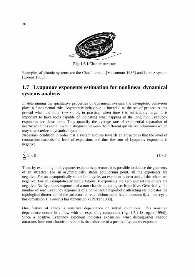
Fig. 1.6.1 Chaotic attractor.
Examples of chaotic systems are the Chua’s circuit [Matsumoto 1985] and Lorenz system
[Lorenz 1963].
1.7 Lyapunov exponents estimation for nonlinear dynamical
systems analysis
In determining the qualitative properties of dynamical systems the asymptotic behaviour
plays a fundamental role. Asymptotic behaviour is intended as the set of properties that
prevail when the time t , or, in practice, when time t is sufficiently large. It is
important to have tools capable of indicating what happens in the long run. Lyapunov
exponents are these tools. They quantify the average rate of exponential separation of
nearby solutions and allow to distinguish between the different qualitative behaviours which
may characterize a dynamical system.
Necessary condition in order that a system evolves towards an attractor is that the level of
contraction exceeds the level of expansion, and thus the sum of Lyapunov exponents is
negative
01
n
ii . (1.7.1)
Then, by examining the Lyapunov exponents spectrum, it is possible to deduce the geometry
of an attractor. For an asymptotically stable equilibrium point, all the exponents are
negative. For an asymptotically stable limit cycle, an exponent is zero and all the others are
negative. For an asymptotically stable k-torus, k exponents are zero and all the others are
negative. No Lyapunov exponent of a non-chaotic attracting set is positive. Generically, the
number of zero Lyapunov exponents of a non-chaotic hyperbolic attracting set indicates the
topological dimension of the attractor: an equilibrium point has dimension 0, a limit cycle
has dimension 1, a k-torus has dimension k [Parker 1989].
One feature of chaos is sensitive dependence on initial conditions. This sensitive
dependence occurs in a flow with an expanding component (fig. 1.7.1 [Strogatz 1994]).
Since a positive Lyapunov exponent indicates expansion, what distinguishes chaotic
attractors from non-chaotic attractors is the existence of a positive Lyapunov exponent.

37
Fig. 1.7.1 Divergence of nearby trajectories in chaotic phenomena.
From the facts that at least one Lyapunov exponent of a chaotic system must be positive,
that one Lyapunov exponent of any limit set other than equilibrium point must be zero, and
that the sum of the Lyapunov exponents of an attractor must be negative, it follows that a
chaotic attractor must have at least three Lyapunov exponents, which implies that an
autonomous chaotic system must have a dimension not less than three. Thus, for a chaotic
attractor, one exponent is positive, one is zero, and all the others are negative.
When more than one Lyapunov exponent of an attractor is positive, then this is called
hyperchaotic behaviour [Rossler 1979]. Hyperchaos normally arises as a natural regime in
extended space-time systems, delayed systems or in complex networks. The first example of
hyperchaotic system was presented by Rossler (Fig. 1.7.2) [Rossler 1979] whereas
hyperchaos was first observed from a physical system by Matsumoto, Chua and Kobayashi
in [Matsumoto 1986].
Fig. 1.7.2 Hyperchaotic Rossler attractor.
1.8 Algorithms for the evaluation of Lyapunov exponents
Unfortunately, Lyapunov exponents are not easy to calculate. The computational load is
considerable, and results are sometimes uncertain due to numeric problems. It is therefore
important to develop efficient algorithms for the calculation of Lyapunov exponents.
Let us consider a n-th order autonomous continuous-time dynamical system defined by the
state equation (1.1.2). The solution is denoted by t(x0), where x0 is the initial state. Let us

38
consider the variation of the solution when the initial conditions are perturbed,
Y(t)=t(x0)/x0, and the Jacobian matrix A(t)=f/x. The equation
IY
YΑY
)(
)()(
0t
ttt (1.8.1)
is called variational equation.
Lyapunov exponents can be evaluated analytically as
t
t
it
it
i dttt
tdt
0
Re1
limlog1
lim , (1.8.2)
where di(t) are the square root of the eigenvalues of YT(t)Y(t) and i(t) are the eigenvalues
of A(t). In presence of at least one positive Lyapunov exponent, the elements of the matrix
YTY diverge [Eckmann 1985]. Moreover, Y
TY is ill-conditioned, because its column vectors
tend to line up along the local direction of most rapid growth. These problems can be
overcome considering the growth rate of n-dimensional volumes [Benettin 1980, Shimada
1979]. These volumes can be computed by QR method applied on integration of system
(1.8.1) [Dieci 1997].
Ad hoc procedures for the numerical calculation of LEs in PWL systems have been
proposed in [Chialina 1994]. In [Parker 1986] a procedure for the solution of the variational
equation in PWL systems is reported.

39
Chapter 2
Nonlinear dynamical systems synthesis
This chapter describes the state of the art concerning on the synthesis of hyperchaos by
coupling of chaotic circuits.
2.1 Generating hyperchaos by coupling of chaotic circuits
Synthesis of hyperchaotic circuits is a fundamental and interesting problem. These systems
do not imply just a realization method of existing mathematical models but important real
physical systems to investigate interesting nonlinear phenomena. Recently, the generation of
hyperchaos and the hyperchaotic circuit realization have attracted the increasing attention of
researchers, and a variety of chaotic and hyperchaotic circuits have been presented.
In order to obtain hyperchaos, three important requirements must be met: dissipative
structure of the system, minimal dimension of the phase space that embeds the hyperchaotic
attractor of the system not less than four, number of terms in the equations giving rise to
instability not less than two, of which at least one must have a nonlinear function. As a
consequence of the requirement on the minimal dimension of the phase space, the minimum
number of coupled first-order autonomous ordinary differential equations must be four.
A simple way to construct a hyperchaotic circuit is to use two or more, regular chaotic
circuits either identical or non-identical ones. They can be coupled by means of linear or
nonlinear resistors by unidirectional or recurrent coupling.
Generally speaking, these hyperchaotic systems have been derived by an ad hoc design
rather than by a systematic procedure. In these cases, the dynamics of coupled chaotic
systems is strictly linked with their synchronization. The method most frequently used for
detecting hyperchaos in this type of systems is based on the evaluation of the Lyapunov
exponents.
In the case of coupled Chua’s circuits, many linear and ring geometries have been
considered in terms of chaotic synchronization. Different theoretical and experimental
results have been obtained, depending on the type of the arrangement. Kapitaniak et al. have
reported experimental observations of hyperchaotic attractors in open and closed chains of
Chua’s circuits [Hu 2011]. In References [Li 2011][Zhang 2010], linear-stability analyses of
a ring of N Chua’s oscillators are performed. Results show that, for a number of oscillators
in the ring that is smaller than a certain critical number, the behaviour of the system is
chaotic synchronized, whereas, above such a threshold value, the system exhibits a
hyperchaotic behaviour consisting in a cycling wave of chaotic amplitude that travels
through the array [Suzuki 1994].
In [Elwakil 2006] unidirectional and diffusive coupling of identical n-double scroll cells in a
one-dimensional cellular neural network is studied. Weak coupling between the cells leads
to hyperchaos, with n-double scroll hypercube attractors.
In [Li 2008], a pair of bi-directionally coupled Chua’s circuits is dealt with. The study
makes reference to PWL Chua’s circuits and shows the existence of hyperchaotic attractors.
In [Grassi 2009] two Chua’s circuit with cubic nonlinearity, bidirectionally coupled, are

40
considered. The dynamics is analysed referring to a transformed space, i.e., the space
described by the transverse and tangent systems. With the proposed coupling, the transverse
system is described by the same equations of a single autonomous system, whereas the
tangent system is structurally identical but forced by the transverse system. In [Kapitaniak
1994] the procedure has been extended to any dynamic system with nonlinear polynomial
elements and it has been tested through application to Chua’s circuit with cubic nonlinearity,
Lorenz system and Rossler system.
In [Lorenzo 1996] hyperchaotic attractors are generated in a ring of three Chua’s circuits
exploiting sine function as nonlinearities, whereas in [Matias 1997] two sinusoidal
oscillators are nonlinearly coupled.
In [Suykens 1997] a hyperchaotic oscillator consisting of two Wien-bridge oscillators
coupled by a resistor and a diode is presented. The whole circuit is investigated both
numerically and experimentally. Also, its hyperchaotic dynamics is studied theoretically by
a topological horseshoe with two-directional expansions which provides an immediate
evidence of hyperchaos.
In [Sanchez 2000] four-wing and eight-wing hyperchaotic attractors are generated by
coupling identical Lorenz systems. The presence of hyperchaos is demonstrated by means of
the calculation of Lyapunov exponents.
Connecting two symmetric three-dimensional linear systems by hysteresis switching
[Cannas 2002] or adding a state-dependent impulsive switching to chaotic system [Cincotti
2007] also leads to the birth of hyperchaos.
In [Cafagna 2003] an experimental and numerical study into the transition between
synchronized low-dimensional, and unsynchronized hyperchaotic dynamics using a system
of coupled electronic chaotic oscillators is presented.
In [Camplani 2009] one of the authors presented two Lorenz systems nonlinearly mutually
coupled obtaining a six-dimensional system with two positive Lyapunov exponents.

41
Chapter 3
Data analysis and statistics
The term “statistics” derives from the Latin word “status,” meaning “state.” Statistics
comprises three major divisions: collection of statistical data, their statistical analysis, and
development of mathematical methods for processing and using the statistical data to draw
scientific and practical conclusions. In this chapter, some concepts concerning with statistics
and statistical methods for data analysis are presented. In addition, some concepts related to
graph theory are introduced.
3.1 Preliminary concepts
Below some preliminary notions of statistics will be introduced ([Polyanin 2007]).
The set of all possible results of observations that can be made under a given set of
conditions is called the population. The population is treated as a random variable X.
Definition 3.1.1: The cumulative distribution function of a random variable X is the
function FX(x) whose value at each point x is equal to the probability of the event {X < x}:
xXPxFxFX . (3.1.1)
The cumulative distribution function has a number of properties:
1. F(x) is bounded: 0 ≤ F(x) ≤ 1.
2. F(x) is a non-decreasing function for ),( x : if x2 > x1, then F(x2) ≥ F(x1).
3. 0)(lim
xFx
.
4. 1)(lim
xFx
.
5. The probability that a random variable X lies in the interval [x1, x2) is equal to the
increment of its cumulative distribution function on this interval:
1221 xFxFxXxP .
6. F(x) is left continuous: )()(lim 00
xFxFxx
.
Definition 3.1.2: A random variable X is said to be continuous if its cumulative distribution
function F(x) can be represented in the form
x
X dyyfxF . (3.1.2)
The function fX(x) = f (x) is called the probability density function of the random variable X.
The probability density function has the following properties:
1. f(x) is always non-negative: f(x) ≥ 0.

42
2. 2
1
21
x
x
dyyfxXxP .
3. 1
dyyf .
4. xxfxxXxP .
5. For continuous random variables, one always has P(X = x) = 0, but the event {X = x} is
not necessarily impossible.
6. For continuous random variables,
)()()()( 21212121 xXxPxXxPxXxPxXxP .
Definition 3.1.3: The expectation (expected value) E{X} of a continuous random variable X
defines the mean position of a random variable and is given by
dxxxfXE . (3.1.3)
For the existence of the expectation, it is necessary that the integral in (3.1.3) converges
absolutely.
Definition 3.1.4: The expectation E{Y} of a continuous random variable Y, which is related
to a random variable X by a functional dependence Y = g(X), can be determined by
dxxfxgXgEYE , (3.1.4)
where f(x) is the probability density function of the random variable X.
Definition 3.1.5: The variance Var{X} of a continuous random variable X is the measure of
the deviation of X from its expectation E{X}, determined by the relation
XEXEdxxfXExXVar 222
. (3.1.5)
Definition 3.1.6: A quantile of level γ of a one-dimensional distribution is a number tγ for
which the value of the corresponding distribution function is equal to γ, i.e.
10 tFtXP . (3.1.6)
All the concepts related to probability distributions of one-dimensional random variables
can be extended to the multidimensional case.
Definition 3.1.7: The distribution function F(x(1)
, x(2)
, …, x(N)
) = FX(1)
, X(2)
, …, X(N) (x
(1), x
(2), …,
x(N)
) of a N-dimensional random vector (X(1)
, X(2)
, …, X(N)
), or the joint distribution function
of the random variables X(1)
, X(2)
, …, X(N)
, is defined

43
as the probability of the simultaneous occurrence (intersection) of the events {X(1)
< x(1)
},
{X(2)
< x(2)
}, …, {X(N)
< x(N)
}, i.e.,
NNN xXxXxXPxxxF ,...,,,...,, 221121 . (3.1.7)
Definition 3.1.8: A multivariate random variable (X(1)
, X(2)
, …, X(N)
) is said to be continuous
if its joint distribution function F(x(1)
, x(2)
, …, x(N)
) can be represented as
N
N
xN
x xN
XXX
N dydydyyyyfxxxF ...,...,,...,...,,
2 1
21
2121
,.. . ,,
21, (3.1.8)
where the joint probability function f(x(1)
, x(2)
, …, x(N)
) = fX(1)
, X(2)
, …, X(N) (x
(1), x
(2), …, x
(N)) is
piecewise continuous.
Theorem 3.1.1: Two random variables X and Y are independent if and only if the joint
distribution function of the bivariate random variable (X, Y) is equal to the product of the
cumulative distribution functions of X and Y, or equivalently, if and only if the joint density
function of the bivariate random variable (X, Y) is equal to the product of the probability
density functions of X and Y
yFxFyxF YXYX ,,, (3.1.9)
yfxfyxf YXYX ,,. (3.1.10)
A set of entities randomly selected from a population is called a sample. A sample must be
representative of the population i.e., it must show the right proportions characteristic of the
population. The number of elements in a sample is called its size and is denoted by the
symbol n. The elements of a sample are denoted by X1, …, Xn.
Definition 3.1.9: The empirical distribution function corresponding to a random ordered
sample X1, …, Xn is defined for each real x by the formula
n
kkn
Xx
XxXnk
Xx
xF
1
0
1
1
* (3.1.11)
i.e., )(* xFn is constant on each interval (Xk, Xk+1] and increases by 1/n at the point Xk. The
empirical distribution function )(* xFn is an unbiased consistent estimator of the theoretical
distribution function i.e., converges to the theoretical distribution function as n .
Definition 3.1.10: Let Hi, i = 1, 2, …, L be the random events that the random ordered
sample X1, …, Xn lies in the ith interval Δi = xi+1 – xi and let ni be their frequencies. The bar
graph consisting of rectangles whose bases are class intervals of length Δi and whose
heights are equal to the relative frequency densities ni/(nΔi) is called the relative frequency
histogram. The area of the relative frequency histogram is equal to . The relative frequency
histogram is an estimator of the probability density function.

44
Definition 3.1.11: The sample mean of a random sample X1, …, Xn is defined as
n
iiX X
n 1
* 1 (3.1.12)
and is an unbiased consistent estimator of the population expectation.
Definition 3.1.12: The sample variance of a random sample X1, …, Xn is defined as
n
iXiXXX X
n 1
2***2
1
1 (3.1.13)
and is an unbiased estimator of the population variance.
Definition 3.1.13: The sample covariance between two random samples X1, …, Xn and Y1,
…, Yn is defined as
n
iYiXiXY YX
n 1
***
1
1 . (3.1.14)
3.2 Some theoretical distributions
In tables 3.2.1 and 3.2.2, a list of theoretical distributions mentioned in the thesis is shown.
For each distribution, the probability density function (table 3.2.1) and the cumulative
distribution function (table 3.2.2) are shown.
3.3 The memorylessness property
The memorylessness property ([Feller 1968]) is related to the conditional behaviour of
random variables related to the time between two subsequent events. Let T be one of those
variables. Suppose we know in advance that the time T between two events is greater than a
fixed value T1. The conditional probability that we need to wait less than another T2 seconds
before the subsequent event, given that the following event has not yet happened after T1
seconds is given by
1
121
1
211121
1Pr
PrPr
TF
TFTTF
TT
TTTTTTTTT
. (3.3.1)
If the probability in (3.3.1) is independent on T1, i.e. if
22121 PrPr TFTTTTTTT , (3.3.2)
then, the distribution is called memoryless.
The exponential is the only memoryless continuous distribution.

45
Table 3.2.1 Probability density function of some theoretical distributions.
Distribution Probability density
function Distribution
Probability density
function
Birnbaum–
Saunders or fatigue
life
x
x
xx
x2
2
2exp
22
0,
Levy
xx 2exp
2 3
0
Burr or
Singh–Maddala 1
1
k
k
x
xk
0,, k
Log–logistic 21
x
x
0,
Chi-squared
2exp
22 2
12 xx
N
Log–normal
2
2
2 2
lnexp
2
1
x
x
R ,0
Dagum 1
1
k
k
x
xk
0,, k
Normal
2
2
1exp
2
1
x
R ,0
Exponential x exp
0
Pearson type
5
xx
exp1
0,
Frechet
xxexp
1
0,
Pearson type
6 21
12
21
1
,
xB
x
0,, 21
Gamma
xxexp
1
0,
Rayleigh
2
2
2 2exp
xx
0
Generalized
gamma
k
k
k xkx
exp1
0,, k
Rice
202
22
2 2exp
xI
xx
0,0
Inverse Gaussian
x
x
x 2
2
3 2exp
2
0,
Weibull
xx exp1
0,

46
Table 3.2.2 Cumulative distribution function of some theoretical distributions.
Distribution Cumulative distribution function Distribution
Cumulative
distribution
function
Birnbaum–
Saunders or
fatigue life
x
x
0,
Levy
x
2
0
Burr or
Singh–
Maddala
k
x
11
0,, k
Log–logistic
1
1
x
0,
Chi-squared
2
22
x
N
Log–normal
xlog
R ,0
Dagum
k
x
1
0,, k
Normal
x
R ,0
Exponential xexp1
0
Pearson type
5
x1
0,
Frechet
xexp
0,
Pearson type
6
21,x
xI
0,, 21
Gamma
x
0,
Rayleigh
2
2
1exp1
x
0
Generalized
gamma
kx
0,, k
Rice
xQ ,1 1
0,0
Inverse
Gaussian
2exp
x
x
x
x
0,
Weibull
xexp1
0,

47
3.4 Maximum likelihood estimation method for unknown
parameters
Maximum likelihood estimation is the most popular estimation method for the estimation of
the parameters of a theoretical distribution. This method allows to estimate the parameters
of a theoretical distribution directly from the sample elements.
Definition 3.4.1: Let the theoretical distribution function F(x) of a population belong to a
family F(x, θ) with unknown parameter vector θ. If the sample elements X1, …, Xn are
drawn independently from the family F(x, θ), then the likelihood function is given by the
joint probability density function of the all sample, and is given by
n
iin XfXXL
11 ,,,..., . (3.4.1)
In the likelihood function, the sample elements X1, …, Xn are known fixed parameters and θ
is an argument. Then, the maximum likelihood estimator is a vector θ* such that the
likelihood function is maximized.
Since L and logL attain maximum values for the same values of the argument θ, it is
convenient to use the logarithm of the likelihood function in practical implementations of
the maximum likelihood method.
The equation
0,log,,...,log1
1
n
iin XfXXL
θθ (3.4.2)
is called the likelihood equation, and its solution vector gives the maximum likelihood
estimator θ* ([Polyanin 2007]).
3.5 Goodness of fit tests
Suppose that there is a random sample X1, …, Xn drawn from a population X with unknown
theoretical distribution function F(x). It is required to test the null hypothesis H0: F(x) =
F0(x) against the alternative hypothesis H1: F(x) ≠ F0(x), where F0(x) is a given theoretical
distribution function. There are several methods for solving this problem that differ in the
form of the measure of discrepancy between the empirical and hypothetical distribution
laws. One of them is the Kolmogorov–Smirnov (K–S) test ([Sachs 1984]).
In the K-S test the measure of discrepancy is a function of the difference between the
empirical cumulative distribution function F*(x) of the experimental data and the theoretical
one F(x) deduced from the model adopted. Relying on the fact that the value of the
empirical cumulative distribution function is asymptotically normally distributed, the K–S
test consists on finding the K-S statistic,

48
xFxFKx
*sup , (3.5.1)
that is the greatest discrepancy between the empirical and theoretical distribution function,
and comparing it against the critical K-S statistic for that sample size. For high n the critical
K-S statistic is given by
2log
5.0
nKcr , (3.5.2)
where α is the significance level, normally equal to 5% or 1%. If
crKK , then the null
hypothesis H0 is rejected at the significance level α.
Other two criterions to test the goodness of fit of a certain empirical distribution with a
theoretical one are the Akaike Information Criterion (AIC) and the Bayesian Information
Criterion (BIC) ([Ljung 1999]).
AIC is a way of selecting a model from a set of models. In this case, the model is the
theoretical distribution. It is defined as
kLAIC 2log2 , (3.5.3)
where L is the likelihood function and k is the number of parameters of the model. Given a
set of candidate models for the data, the preferred model is the one with the minimum AIC
value. Hence AIC not only rewards goodness of fit, but also includes a penalty that is an
increasing function of the number of estimated parameters. This penalty
discourages overfitting.
BIC is a criterion alternative to AIC. It is defined as
nkLBIC lnln2 , (3.5.4)
where n is the number of samples. Also for BIC, given a set of candidate models for the
data, the preferred model is the one with the minimum BIC value. The fitted model favoured
by BIC ideally corresponds to the candidate model which is a posteriori more probable.
There is also a graphical method, known as the quantile-quantile (Q-Q) plot, used for
comparing the empirical and theoretical probability distributions. In a Q-Q plot, the
quantiles of the sample are plotted against the quantiles of the theoretical distribution. If the
two sets come from a population with the same distribution, the points should fall
approximately along a 45-degree reference line. The greater the departure from this
reference line, the greater the evidence for the conclusion that the sample set have come
from a population with a different distribution. An example of Q-Q plot is given in fig.
3.5.1.

49
Fig. 3.5.1 Example of Q-Q plot for a sample taken from a population with normal
distribution.
3.6 Analysis of variance
All techniques previously shown are useful for the statistical analysis of a given sample and
for the extrapolation from it of theoretical information about the population from which the
sample was extracted. In the case of presence of different samples, it is important to
understand if these samples come from the same population or from different populations.
The technique typically used to decide whether the different samples belong to the same
population is the one-way analysis of variance (ANOVA) ([Polyanin 2007], [Dowdy 2004]).
Using this technique, the variation between different sample means is used to estimate the
variation between individual observations. Suppose that there are L independent samples
X1,1, …, Xn1,1; X1,2, …, Xn
2,2; …; X1,L, …, Xn
L,L, drawn from normal populations with unknown
expectations a1, …, aL and unknown but equal variances σ2. It is necessary to test the null
hypothesis H0: a1 = …= aL that all theoretical expectations ai are the same against the
alternative hypothesis H1that some theoretical expectations are different. It should be noted
that this test can be performed given the assumption that each parent population is normally
distributed and have the same variance.
If the hypothesis that all samples belong to a population having a normal distribution cannot
be met, because for example the elements of samples are all positive quantities which cannot
be described by a distribution defined also for negative values, an alternative method is
necessary. A method useful for this purpose is the Kruskal-Wallis test ([Kruskal 1952],
[Davis 2002]). This test makes no assumption about the distribution of samples, but requires
to use ranks instead of the original observations, that is to array all the observations in order
of magnitude and replace the smallest by 1, the next-to-smallest by 2, and so on; if there are
ties (two or more equal observations), each observation is given the mean of the ranks for
which is tied. The test statistic to be computed is
TNN
Nn
R
H
L
i i
iNN
3
1
2
112
11
13
, (3.6.1)
50
where L is the number of samples, ni is the number of observations in the ith sample, N is
the number of all observations, Ri is the sum of the ranks in the ith sample, the sum in the
denominator is over all groups of ties and T = t3 – t for each group of ties, t being the
number of tied observations in the group. If the samples come from identical continuous
populations, for high ni, H is approximately distributed as 2 (chi-squared distribution) with
L – 1 degrees of freedom. Thus the critical H statistic is given by
11FHcr , (3.6.2)
where α is the significance level and F-1
(x) is the inverse cumulative distribution function of
a chi-squared distribution with L – 1 degrees of freedom. If
crHH , then the null
hypothesis H0, whereby the samples come from the same population, is rejected at the
significance level α.
3.7 Graph theory and clique detection
In computer science, the clique problem refers to any of the problems related to finding
particular complete subgraphs ("cliques") in a graph, i.e., sets of elements where each pair
of elements is connected.
Let G = (V, E) be an arbitrary undirected graph, where V = {1, 2, …, nV} is the node set of G
and E V V is the edge set of G. The symmetric nV nV matrix AG = (ai,j)(i, j)VV, where
ai,j = 1 if (i, j) E is an edge of G, and ai,j = 0 if (i, j) E, is called the adjacency matrix of
G. Suppose that all the diagonal entries of the adjacency matrix are zero, i.e. no edge has
both ends connected to the same node. Thus, the adjacent matrix AG is a symmetrical matrix
with zero diagonal entries.
In [Harary 1957] the adjacency matrix is called the group matrix, and the graph edges
represent the presence of an interpersonal relationship among members of a group. This
concept can be generalized to a generic set of elements among which we wish to study the
presence or absence of a particular relationship. Then, a clique is a maximal subgraph of at
least three nodes in which each node is connected by an edge to each other node.
Harary et al. have proposed an algorithm [Harary 1957] for finding cliques in a social group.
The algorithm, which is summarized below, can be generalized to a general graph. For this
purpose some definitions are needed. A noncliqual node is one who does not belong to any
clique. A unicliqual node is one who belongs to exactly one clique. A multicliqual node
belongs to more than one clique. Two nodes are cocliqual if they belong both to at least one
clique.
Step 1. Given a graph G, the matrix AG2 AG is constructed, where represents the
elementwise product operator. The i, j entry of this matrix is zero if and only if nodes i and j
are not cocliqual, and is positive otherwise. Consequently, all those graph nodes whose row
in AG2 AG consists entirely of zeros are noncliqual. Let MG be the submatrix of AG
2 AG
obtained by deleting from it the rows and columns corresponding to every noncliqual node.
The sum of the elements in any row of MG is equal to the corresponding diagonal element of
AG3. After calculating the matrix MG, the rows of MG are examined. Let v be any node
whose row sum in MG is r(v). Then, if and only if r(v) = n(v) [n(v) – 1], where n(v) is the
51
number of nodes cocliqual with v, i.e. the number of positive elements in v’s row in MG, V is
a unicliqual node. If G contains unicliqual persons, proceed to step 2, else skip to step 4.
Step 2. Having the unicliqual node v, the next step is to find the clique Cv to which v
belongs, and the set Cv’, which denotes the set of all unicliqual nodes in Cv. The clique Cv
consists of v, together with all those nodes whose entry in v’s row in MG is not zero.
Step 3. If Cv = G, then G has only one clique. In this case skip to step 5. Else, if Cv G, let
G = G – Cv’ and revert to step 1.
Step 4. The graph G contains no unicliqual nodes, and the matrix MG has been already
calculated in step 1. Let v be any member of G such that r(v) is minimal. The next step is to
find the subgraphs G(v) and G(–v), where G(v) consists of v and all nodes cocliqual with v
and G(–v) consists of the nodes in cliques not containing v.
Step 5. On arriving at this step from step 4, we now have the two subgraphs G(v) and G(–v).
Send one of these to to step 1 and store the other. When arriving from step 3, send any
stored subgroup to step 1. If there are no subgroups in storage, the preocedure is terminated.
Some of the noncliqual nodes can be isolated nodes, i.e. nodes with no edges. The other
noncliqual nodes may be connected with another node, which can be noncliqual, unicliqual
or multicliqual, forming a “pair” of nodes.


53
Chapter 4
Nonlinear time series analysis
Deterministic dynamical systems, describe the time evolution of a system in some phase
space. They can be expressed for example by ordinary differential equations or in discrete
time by difference equations. A time series can then be thought of as a sequence yn of N
observations performed with some measurement function at successive time instants spaced
at uniform time intervals.
Time series analysis includes methods for analysing time series data in order to extract
meaningful statistics and other characteristics of the data. Methods for time series analyses
may be divided into two classes: frequency-domain methods and time-domain methods. The
first include spectral analysis and wavelet analysis; the second include auto-correlation and
cross-correlation analysis.
Below an overview on the wavelet transform and its application for the denoising of noisy
signals (sections 4.1, 4.2), and on the use of auto-correlation and cross-correlation analysis
(section 4.3) has been reported. Moreover, some useful methods for the reconstruction of the
phase space and for the identification of parameters from a time series has been shown
(sections 4.4, 4.5, 4.6). Finally some methods for the evaluation of Lyapunov exponents to
test the chaoticity of time series (section 4.7) and an introduction to the use of the Hurst
exponent to give a measure of the long term correlation in a time series (section 4.8) have
been reported.
4.1 Wavelet transform
The development of Fourier analysis is based on the properties of periodic functions, which
can be expressed as an infinite sum of trigonometric functions. These basic functions have
the key property of localization in frequency. The Windowed Fourier Transform (also
known as the short-time FT), in attempting to overcome this deficiency, provides a two-
dimensional representation in the time-frequency domain windowing the signal. However,
resolution in both time and frequency remains constant because the same window is
employed across the entire frequency range. Such conventional transforms, which employ
continuous periodic basis functions, are not suitable to characterize non-periodic and
transient signals.
The wavelet transform is a mathematical tool that can simultaneously provide information
on time and frequency of a signal, contrary to what happens with trigonometric functions. It
works on specific parts of a signal to extract local structures and singularities. This makes
the wavelets ideal for handling non-stationary and transient signals, as well as fractal-type
structures ([Han 2006][Han 2009][Wornell 1992][Staszewski 1999]).
The Continuous Wavelet Transform (CWT) of a signal )(ty is defined as follows ([Chen
2003]):
dtttysCWT sy ,, (4.1.1)
54
where the wavelet function
s
t
sts
1, (4.1.2)
is a dilated and translated version of the Mother Wavelet )(t , s is the scale parameter,
is the translation parameter and * represents the complex conjugate operator. The term
"wavelet" means small wave, because of the block-wave form of )(t . The term "mother"
implies that the functions used in the transformation process are derived from one main
function, the mother wavelet. Literature reports a number of analytical mother wavelets.
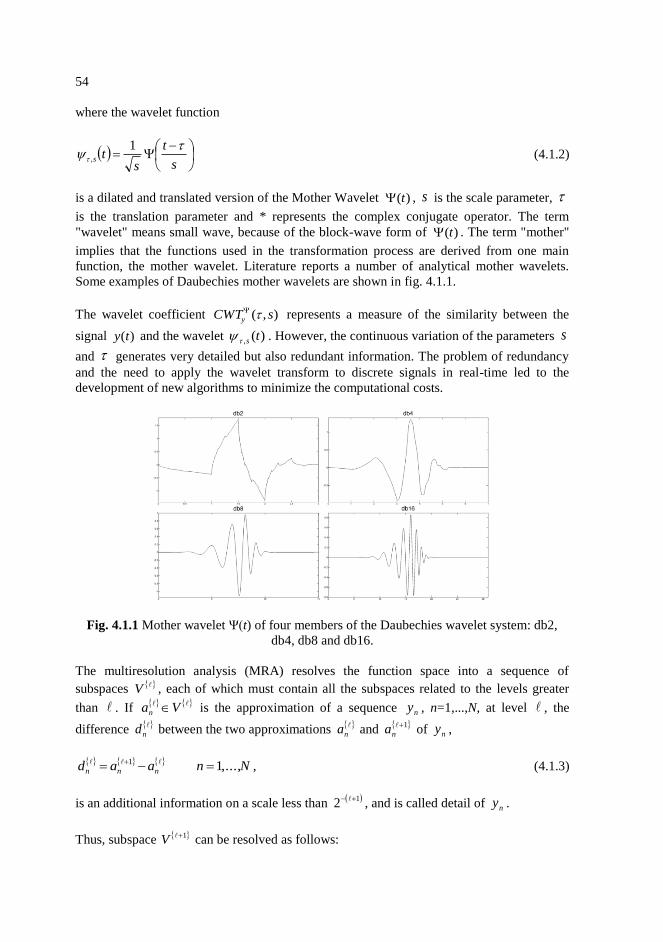
Some examples of Daubechies mother wavelets are shown in fig. 4.1.1.
The wavelet coefficient ),( sCWTy represents a measure of the similarity between the
signal )(ty and the wavelet )(, ts . However, the continuous variation of the parameters s
and generates very detailed but also redundant information. The problem of redundancy
and the need to apply the wavelet transform to discrete signals in real-time led to the
development of new algorithms to minimize the computational costs.
Fig. 4.1.1 Mother wavelet Ψ(t) of four members of the Daubechies wavelet system: db2,
db4, db8 and db16.
The multiresolution analysis (MRA) resolves the function space into a sequence of
subspaces V , each of which must contain all the subspaces related to the levels greater
than . If Van is the approximation of a sequence ny , n=1,...,N, at level , the
difference nd between the two approximations
na and
1na of ny ,
Nnaad nnn ,...,11
, (4.1.3)
is an additional information on a scale less than 12
, and is called detail of ny .
Thus, subspace 1V can be resolved as follows:

55
WVV 1 (4.1.4)
where the space W , orthogonal to V , is called detail space and represents the
operator sum of vector spaces. By means of a scaling function Φ, called Father Wavelet, the
bases k are generated for each subspace:
knnk
22 2 . (4.1.5)
Equation (4.1.5) is known as dilation equation.
Similarly, by means of the Mother Wavelet )(t , the bases k are generated for each
subspace W :
knnk
22 2 . (4.1.6)
Equation (4.1.6) is known as wavelet equation.
Generally speaking, using the mother and the father wavelets, a signal ny can be written as
follows:
0
0
0
0
11,
nn
kkk
kkkn danny , (4.1.7)
where 0 is the level of decomposition, k are the approximation coefficients at resolution
level 0 , ,k are the detail coefficients at level . In the case of orthogonal bases, the
coefficients are calculated with the following expressions:
iii
iik kyiky 00
0
22 2
(4.1.8)
iii
iik kyiky
22 2, . (4.1.9)
The coefficients ,k and k give the Discrete Wavelet Transform (DWT) of the signal ny .
The expression of DWT is similar to the general equation of a FIR digital filter.
The DWT can be easily implemented by using the pyramid algorithm. The algorithm uses
two digital filters, a high-pass filter hn and a low-pass filter gn, which give rise to a bank of
filters able to decompose the signal into low and high frequency components, by means of
undersampling operations by a factor of two (fig. 4.1.2a). The series of filtering operations
at different frequencies correspond to a signal analysis at different resolution levels. This
process can be expressed completely in terms of the digital filters gn and hn as follows:

56
kknkn
kknkn
aha
agd
2
1
2
1
. (4.1.10)
Fig. 4.1.2 Filter bank of decomposition (a) and reconstruction (b).
The signal reconstruction is achieved by inverting the decomposition procedure (fig. 4.1.2b).
The approximation and the detail at each level are oversampled by a factor of two, then
filtered by a high-pass filter nh and a low-pass filter ng respectively, and finally summed,
to give the approximation at lower level.
4.2 Denoising by thresholding of wavelet coefficients
Most noise reduction algorithms assume that noise ηnwith zero mean is added to a discrete
signal yn of N data points, giving an experimental signal which can be written as:
nnn ηyz (4.2.1)
The linearity of the wavelet transform preserves the additivity of the model:
kkk ωvw (4.2.2)
where wk are the noisy signal wavelet coefficients, vk are the uncorrupted wavelet
coefficients, ωk are the noise wavelet coefficients.
Since noise is often spread out equally over many coefficients, if the signal energy is
concentrated in a small number of wavelet coefficients, its coefficient values will be
relatively large compared to those of the noise. Thus, a good denoising methodology using
wavelets is thresholding ([Donoho 1994]).
Thresholding is a simple non-linear technique, which operates on one wavelet coefficient at
a time. In its most basic form, each coefficient is compared to a threshold: if the coefficient
is smaller than the threshold, it is set to zero; otherwise, it is kept (hard thresholding) or

57
shrunk (soft thresholding). The difference between hard and soft thresholding is shown in
fig. 4.2.1.
Fig. 4.2.1 Noise reduction by wavelet thresholding. (a) Hard-thresholding (b) Soft-
thresholding. The x axis represents the original wavelet coefficients, the y axis the values
computed by the thresholding procedure.
The main problem of noise reduction by thresholding wavelet coefficients is to find the best
threshold that allows eliminating only the noise and leaves the signal unaltered. Two aspects
must be considered. First of all, in general, signals have different characteristics at different
scales and, if the noise is correlated instead of white, also the noise behavior depends on the
resolution.
Secondly, one single threshold cannot efficiently remove noise, if the amount of noise
depends on the resolution level, or the signal has different characteristics at different scales.
Thus, scale-dependent thresholds are generally the best solution. A small threshold yields a
result close to the input, but the resulting signal may still be noisy. Conversely, a large
threshold produces a signal with a lot of zero wavelet coefficients and can alter the signal.
The scale-dependent thresholds have to be chosen to optimize a given cost function.
Signal denoising using wavelet transforms consists of three steps, namely, signal
decomposition, thresholding of the wavelet coefficients, and signal reconstruction. The
wavelet transform of the noisy signal up to a given level 0 is evaluated. Then, the detail
coefficients in the different levels are thresholded and the denoised signal is obtained
through the inverse of the wavelet transform.
In [Donoho 1994], a universal threshold is proposed
Nln2̂ , (4.2.3)
where 6745.0ˆ M is a rough estimate of the noise level and M is the median absolute
deviation of the detail coefficients up to the level 0 .
In [Han 2006], two scale-dependent thresholding schemes are proposed
Nln2 (4.2.4)
and

58
0
0
0
ln2
1,...,2ln21ln
1ln2ˆ
0
N
N
N
, (4.2.5)
where and are respectively the threshold and the standard deviation of detail
coefficients at scale . The authors set 40 in the two examples. However, the basis to
choose the decomposition level 0 has not been addressed in the paper. On the other hand,
this is a crucial issue since denoising performance may vary with 0 .
In [Han 2009], the approximate coefficients are handled by the Singular Spectrum Analysis
and the details are analyzed combining Singular Spectrum Analysis and Spatial Correlation
theory. In this case, the optimal wavelet decomposition scale is determined by evaluating the
noise residual ratio at different levels and selecting the level with minimum ratio. However,
this procedure cannot be applied when the noiseless signal is unavailable.
In a recent paper, Gao et al. ([Gao 2010]) compare the performance of their algorithm based
on adaptive filtering with those obtained using wavelet thresholding techniques reported in
[Donoho 1994] and [Han 2006]. The authors claim that adaptive filtering is more effective
than wavelet based methods.
4.3 Auto-correlation and cross-correlation analysis
In the analysis of time series it is often very important to measure the dependence of a given
measurement on its predecessors. The auto-covariance is a simple statistical quantity which
measures this dependence. For a time series ny of length N the auto-covariance at lag k is
given by
kN
ikkikik yy
kNac
11
1
(4.3.1)
where there are only N – k elements to compare and the factor N – k – 1 depends on the
correction for the degrees of freedom used in computing the sample auto-covariance. There
is also a particular definition, which considers only a subset of the time series, for the means
to subtract
kN
iik y
kN 1
1
(4.3.2)
N
kiik y
kN 1
1
(4.3.3)

59
Theoretically, it could be possible to increase the lag k until it is large as N – 1, but as the lag
becomes larger, the degree of overlap N – k becomes smaller. Conventionally, the auto-
covariance is evaluated for lags from 0 to about N/4. The resulting values can be displayed
as an auto-covariogram or auto-covariance function, which is a plot of auto-covariance
against lag. The largest value of the auto-covariance is generally, except in the case of
periodic time series, at zero lag, since the series will never perfectly match up except at zero
lag. The zero crossing in the auto-covariance is an important concept, since it characterizes
the length of time that must elapse before the times series becomes uncorrelated. The first
zero is known as the decorrelation time.
The measurement units of auto-covariance are the squares of those of the time series, thus
the auto-covariance is sensitive to the changes of the time series, which makes it difficult to
compare two auto-covariograms. By dividing the auto-covariance by a standardizing factor,
it is possible to compute the so-called auto-correlation
kk
kk
acar
, (4.3.4)
where k
and k
are the standard deviations
kN
ikik y
kN 1
2
1
1
(4.3.5)
N
kikik y
kN 1
2
1
1
. (4.3.6)
The resulting values of the auto-correlation can be displayed as an auto-correlogram, which
is a plot of auto-correlation against lag. The largest value of the auto-correlation is
generally, except in the case of periodic time series, at zero lag, and its value is equal to 1. In
correspondence of the other lags, the auto-correlation oscillates between -1 and 1.
The expected auto-correlation of a random series is zero for lags greater than zero. The
expected standard deviation in the auto-correlation of a random sequence at any lag is
3
1
kNk . (4.3.7)
The value 3 comes from a correction for the degrees of freedom used in computing the
means of each of the two series used (even if they are the same) and in the choice of the
starting point of the autocorrelation. Thus, if
03
96.1
k
kNra k (4.3.8)
then the series is likely (at about 95%) non-random.
60
If it is possible to compare a time series with itself at successive lags, it is possible to
compare two different time series with each other in order to determine positions of
pronounced correspondence. Similarly for the auto-correlation, it is possible to evaluate the
cross-correlation of two time series ny ,1 and ny ,2
kk
kk
cccr
,2,1 , (4.3.9)
where
kN
ikkikik yy
kNcc
1,2,2,1,1
1
1
(4.3.10)
is the cross-covariance at lag k of ny ,1 and ny ,2 , and
kN
iik y
kN 1,1,1
1
(4.3.11)
N
kiik y
kN 1,2,2
1
(4.3.12)
kN
ikik y
kN 1
2
,1,1,11
1
(4.3.13)
N
kikik y
kN 1
2
,2,2,21
1
(4.3.14)
are the mean values and the standard deviations of the two overlapping series ([Davis
2002]).
Like the auto-correlation function, it is possible to test the significance of the cross-
correlation. Thus, if
03
96.1
k
kNcrk (4.3.15)
then the series are likely (at about 95%) cross-correlated ([Box 1970]).
4.4 State reconstruction by differential algebra
Consider a nonlinear time invariant dynamical system described by
ppxgp
ppxfpx
,,,
,,,
tty
tt
(4.4.1)

61
where x is the n-dimensional state variable vector, y is a scalar output function of the state, f,
g, are algebraic vector functions in x, and the dependence on time t and parameter vector p
has been made explicit. This class of systems includes an extensive variety of systems,
including chaotic systems such as Rossler, Lorenz and Chua systems.
We assume that only one scalar output is measured as y(t) (i.e., the state is not directly
available). Since the usually scalar time series in itself does not properly represent the
multidimensional phase space of the dynamical system, some technique to reconstruct the
system state or to unfold the multidimensional structure by using only the information
contained in y(t) must be employed.
Definition 4.4.1 [Forsman 1992]: An algebraic observer for the state xi of the system
(4.4.1) is a polynomial P(xi, y, y(1)
, …, y(m)
) with m < n.
The two following statements are equivalent:
i) the state of the system (1) can be reconstructed;
ii) a smooth function h exists such that x = h(y, p).
The possibility that ii) is verified, is strictly linked to the observability concept. In case of
algebraic systems the most natural way is to refer to algebraic observability [Ljung 1994]
[Fliess1993].
The above property can be easily tested in the differential algebra context by resorting to the
concept of characteristic set associated to the dynamic equations. The characteristic set has
been introduced by Ritt [Ritt 1950] in 1950 and starting from 1990 has been widely used in
the study of the dynamic systems [Ljung1994][Fliess 1993]. In order to define the
characteristic set we need to introduce some concepts of differential algebra. A detailed
formal description of differential algebra can be found in [Ritt 1950].
Remark 4.4.1 [Forsman 1992]: The peculiarity of the characteristic set is that it
summarises all the information contained in the differential equations defining the dynamic
system. In order to handle differential polynomials (polynomials on x and their derivatives)
a ranking of the variables and their derivatives must be introduced.
Chosen the ranking
n
nnnn
n xxxxxxxyyy ............... 22
1
11
11
1
for a system in the form (4.4.1), the characteristic set exhibits n+1 differential polynomials
i.e.:
i. an output relation that is a differential polynomial on y and its derivatives, which can be
expressed as iiappyyyzyk ,...,,...,,,),( 21p , where ai are coefficients
depending on the set of parameters p, and i are polynomial functions in y and its
derivatives.
ii. n differential polynomials triangularised with respect to the state component denoted by
the n-dimensional K(x ,y , p).

62
Remark 4.4.2 [Ljung 1994]: The state space description of the dynamic model ensures the
uniqueness of the characteristic set of the differential polynomials of eqs. (4.4.1).
Property 4.4.1 [Forsman 1992]: A system is algebraically observable if one at least of the
following equivalent relations is verified:
i. derivatives of the state components do not appear in the characteristic set;
ii. k(y, p) is of order n.
Let’s now return to the nonlinear time invariant dynamic system described by the equations
(4.4.1) with initial conditions x(0) = x0. The state x(t, x0) is not directly available, only an
output is measured, say txty i where i = 1, …, n. The goal is the reconstruction of
system state by using only the information contained in y. In order to get k(y, p) and K(x, y,
p) we need to calculate the characteristic set associated to the dynamic equations (4.4.1).
Proposition 4.4.1: A necessary condition for the finite-time global state reconstruction of
the system (4.4.1) is that it is algebraically observable.
If the system is not algebraically observable the characteristic set contains some derivatives
of the state components, hence the state vector is a solution of a differential system whose
initial conditions are unknown. Thus Remark 4.4.1 implies that no further information is
available and the state admits infinite solutions. Conversely if the system is algebraically
observable such solutions are finite in number.
Proposition 4.4.2: The state can be locally reconstructed in a finite time if the system is
algebraically observable and the characteristic set equations K(x, y, p) = 0 have, for x, a
finite number of solutions.
Proposition 4.4.3: The state can be globally reconstructed in a finite time if the system is
algebraically observable and the characteristic set equations K(x, y, p) = 0 have, for x, a
unique solution.
In this case, with the possibility of choosing between a finite number of solutions, the proper
solution depends to the knowledge of a basin of attraction of the initial point.
In the adopted definition of observability only the information contained in the dynamic
equations has been considered without taking into account the initial conditions.
Nevertheless in a physical system such initial conditions, although unknown, are fixed, thus
yielding the following remark.
Remark 4.4.3: Although a system is observable following the Definition 3.4.1, it can
happen that the differential polynomial multiplying some state component in the
characteristic set, let be G(y, y(1)
, y(2)
, …, y(n)
) such polynomial, identically vanishes in the
solution related to a particular initial point. In this case although the system is observable
in the sense of Forsman, such state component would not be reconstructible. This cannot
happen for a generic initial point, indeed vanishing of G (y, y(1)
, y(2)
, …, y(n)
)x(t0) = x
0, for all t
and a generic x0 implies y is identically equal zero.

63
In some cases, the algebraic observability can be easily detected by simple inspection and
manipulation on dynamic equations.
4.5 Identifiability
Algebraic observability is essential for the verification of identifiability of parameters of a
given system. The property of global identifiability allows one to obtain the values of all
parameters by means of the only output and its derivatives.
Proposition 4.5.1: A system of the form (4.4.1) is globally identifiable if and only if, for at
least a generic set of parameters, the equation a(p) = a(p*) has at most a finite number of
solutions {p = p*}. This equation is solved in the set of parameters p.
The procedure to investigate the observability and identifiability property may result rather
complex, hence resorting to a software for calculating the characteristic set is necessary. The
software tool used is DAISY ([Bellu 2007]), it has been written in Reduce 3.6 and resorts to
the Buchberger algorithm for the calculation of Gröbner bases.
4.6 State reconstruction by embedding
An alternative phase space reconstruction technique, especially when the equations of the
dynamic system are not known, is the method of delays. By means of this method, vectors in
a new space, the embedding space, are formed from time delayed values of the scalar
measurements yn
nmnmnn yyy ,...,, 21 s , (4.6.1)
where the number m of elements is called the embedding dimension and the time τ is
generally referred to as the delay.
Embedding theorems by Takens ([Takens 1981]) and by Sauer et al. ([Sauer 1991]) state
that if the sequence {sn} consists of scalar measurements of the state of a dynamical system,
then under certain genericity assumptions, the time delay embedding provides a one-to-one
image of the original set, provided m is large enough.
There is a large literature on the “optimal” choice of the embedding parameters m and τ. It
turns out, however, that what constitutes the optimal choice largely depends on the
application. An implementation of this algorithm can be found in the TISEAN package
([Hegger 1999]) and in [Mohammadi 2009].
4.7 Lyapunov exponents estimation for nonlinear time series
analysis
Since a positive Lyapunov exponent is a strong signature of chaos, it is of considerable
interest to determine its value for a given time series.

64
The first algorithm for this purpose was suggested by Wolf et al. [Wolf 1985].
Unfortunately, this algorithm does not allow one to test for the presence of exponential
divergence, but just assumes its existence and thus yields a finite exponent for stochastic
data also, where the true exponent is infinite, giving easily rise to wrong results.
While Wolf's algorithm does not use more than a delay reconstruction of phase space, there
is another class of algorithms [Sano 1985] [Eckmann 1986] which also involves the
approximation of the underlying deterministic dynamics. This method is very efficient if the
data allow for a good approximation of the dynamics.
In [Rosenstein 1993] and [Kantz 1994] a more robust algorithm, which has been
implemented in the TISEAN package ([Hegger 1999]), has been introduced. It tests directly
for the exponential divergence of nearby trajectories and thus allows to decide whether it
really makes sense to compute a Lyapunov exponent for a given data set. Given a time
series and the embedding parameters, the algorithm firstly reconstructs the attractor with the
method of delays and then, given a point in the embedding space and its neighbourhood,
evaluates the average divergence of the neighbours with respect to the reference point as a
function of time and for N reference points. The size of the neighbourhood should be as
small as possible, but large enough such that on average each reference point has at least a
few neighbours ([Kantz 2004]).
The computation of the full Lyapunov spectrum requires considerably more effort than the
computation of the maximal exponent. An algorithm for this purpose has been implemented
in the TISEAN package. An essential part of this algorithm is some estimate of the local
Jacobians which rules the growth of infinitesimal perturbations ([Sano 1985][Eckmann
1985]). Then Jacobians are multiplied one by one, following the trajectory, to an arbitrary
number of different vectors in tangent space to compute Lyapunov exponents. Every few
steps, a Gram-Schmidt orthonormalization procedure is applied to the set of vectors, and the
logarithms of their rescaling factors are accumulated. Their average, in the order of the
Gram-Schmidt procedure, give the Lyapunov exponents in descending order. A
disadvantage of this method is that it assumes that there exist well defined Jacobians, and
does not test for their relevance [Hegger 1999].
4.8 Hurst exponent
The Hurst exponent occurs in several areas of applied mathematics, including fractals and
chaos theory, long memory processes and spectral analysis. Hurst exponent estimation has
been applied in areas ranging from biophysics to computer networking. It has reached high
popularity especially in the analysis of financial market indexes and stock market ([Lo
2001][Peters 1994]).
Estimation of the Hurst exponent H was originally developed in hydrology and was
introduced by Hurst in [Hurst 1951], when he was studying the historical data of the
flooding of the river Nile.
This quantity can be used to discriminate between a time series generated by a random
process or a long term correlation time series.

65
H ≈ 0.5 indicates a random walk (a Brownian time series). In a random walk there is no
correlation between any element and a future element and there is a 50% probability that
future return values will go either up or down. Series of this type are hard to predict.
0 < H < 0.5 indicates an anti-persistent behaviour. This means that an increase will tend
to be followed by a decrease (or a decrease will be followed by an increase). This
behaviour is sometimes called "mean reversion" which means future values will have a
tendency to return to a longer term mean value. The strength of this mean reversion
increases as H approaches 0.
0.5 < H < 1 indicates "persistent behaviour", that is the time series is trending. This
means that an increase will tend to be followed by an increase. The same is true of
decreases, where a decrease will tend to follow a decrease. The larger the H value is, the
stronger the trend. Series of this type are easier to predict than series falling in the other
two categories.
There are several ways to formally define the Hurst Exponent. The description developed by
Hurst himself is as follows:
H
nn
n
nn
nCn
S
RE
limlimlim , (4.8.1)
where n is also known as the expected value (among the first n samples) of the rescaled
range (R/S), Rn is defined on a time series yn as
niyniyR iin ,...,1,min,...,1,max , (4.8.2)
Sn is the standard deviation of the first n samples and C is an arbitrary constant.
Thus, for every size n, the rescaled range is estimated and the expected value n among the
first n samples is evaluated. This leads to a system of equations
H
n Cn , (4.8.3)
and therefore
nHCn logloglog . (4.8.4)
Using more than two different n, system (4.8.4) is generally over-determined, provided there
is enough input data and can be solved using a least squares fit. The slope of the fit will be
the estimated value for H.


67
Chapter 5
Artificial Neural Networks
Artificial Neural Networks (ANNs) or simply Neural Networks (NNs) derive their
inspiration from the biological neuron system and the brain. The field of neural networks
has a long history of development. Their history begins in the early 1940’s and thus nearly
simultaneously with the history of programmable electronic computers. During the past few
years, ANNs have been successfully applied in several fields, like system identification and
control, chemistry, decision making, pattern recognition, sequence recognition, medical
diagnosis, financial applications, data mining, visualization and e-mail spam filtering. From
a practical point of view, they’ve been used mainly for different tasks, like regression
analysis, classification problems, data processing and robotics. In this chapter an
introduction to neural networks is given, with particular attention to Multi-Layer
Perceptrons (MLPs).
5.1 Components of artificial neural networks
A neural network can be defined as a network that resembles the functional architecture of
the brain. It consists of simple processing units, the neurons, and directed, weighted
connections between those neurons. The first artificial neuron was first proposed by Warren
McCulloch and Walter Pitts in 1943 [McCulloch 1943]. The neuron model is shown in fig.
5.1.1.
Fig. 5.1.1 Basic artificial neuron.
The k-th artificial neuron given in fig. 5.1.1 has p input, denoted as x1, x2, …, xp. The line
connecting input i to the neuron is characterized by a weight, which is denoted as wk,j.
Weights in the artificial model correspond to the synaptic connections in biological neurons.
The threshold, or bias, in artificial neuron is usually represented by ϑk . The activation vk is
given by the formula
k
p
jjjkk xwv
1, . (5.1.1)
The output value of the neuron is a function of its activation
k
T
kkk vy xw , (5.1.2)

68
where the weighted sum in (5.1.1) is expressed in vector notation. The most commonly used
activation functions are the threshold function, the sigmoid function, the hyperbolic tangent
function and the linear function (see table 5.1.1).
Table 5.1.1 Activation functions.
Threshold Sigmoid Hyperbolic tangent Linear
01
00
z
zz
z
z
exp1
1
zz tanh
zz
McCulloch and Pitts proved that a synchronous assembly of such neurons is capable in
principle to perform any computation that an ordinary digital computer can, though not
necessarily so rapidly or conveniently ([Hertz 1991]). In fact, while a single artificial neuron
is not able to implement some complex functions, connecting the outputs of some neurons
as input to the others, so constituting a neural network, may overcome this problem.
5.2 Network topologies
According to the structure of the connections, networks may be basically distinguished for
their architectures: feed-forward, recurrent and competitive neural networks.
In feed-forward neural networks, the neurons are organized in the form of layers. The
neurons in a layer get input from the previous layer and feed their output to the next layer. In
this kind of networks, connections to the neurons in the same or previous layers are not
permitted. The last layer of neurons is called the output layer and the layers between the
input and output layers are called the hidden layers. The input layer is made up of special
input neurons, transmitting only the applied external input to their outputs. In a network if
there is only the layer of input nodes and a single layer of neurons constituting the output
layer then they are called single layer network. If there are one or more hidden layers, such
networks are called multilayer networks. Classical examples of this kind of networks are the
Adaline [Widrow 1960] and the Multi-Layer Perceptron [Cybenko 1992].
The structures, in which loops and feedback connections between neurons belonging to
different layers are allowed, are called recurrent networks. Examples of recurrent networks
are the Elman networks [Elman 1990] and the Hopfield networks [Hopfield 1982].
The third category comprises competitive networks, in which neighbouring cells compete in
their activities by means of mutual lateral interactions, and develop adaptively into specific
detectors of different signal patterns. This kind of network is competitive in the sense that
all the neurons of the network receive the same input. The neuron with the best output
(following a certain criteria) is chosen as the winner. In case of hard competition only one
winner can exist and only its connections weights are updated. In case of soft competition

69
also the neighbours neurons of the winner are involved during the weights update procedure.
An example of competitive network is the Self Organizing Map (SOM) [Kohonen 1990].
5.3 The learning paradigms
The most interesting characteristic of neural networks is their capability to familiarize with
problems by means of training and, after sufficient training, to be able to solve unknown
problems of the same class. This approach is referred to as generalization.
Learning is the procedure that extracts the information from input data. An incomplete
learning leads to a network that does not perform well. There are three main categories of
learning paradigms: unsupervised, reinforcement and supervised learning.
Unsupervised learning is also known as clustering. It provides only input patterns to the
network, which tries to identify similar patterns and to classify them into similar categories
without any a priori information about data distribution.
In reinforcement learning the network receives a logical or a real value after completion of a
sequence, which defines whether the result is right or wrong.
Supervised learning methods provide training patterns together with appropriate desired
outputs. Thus, for each training set that is fed into the network, the output, for instance, can
directly be compared with the correct solution and the network weights can be changed
according to their difference. The objective is to change the weights so that the network can
associate input and output patterns independently after the training, and also provide
plausible results to unknown similar input patterns, i.e. it generalises ([Kriesel 2007]).
5.4 The perceptron
The perceptron was described by Frank Rosenblatt in 1958 [Rosenblatt 1958]. The
perceptron is a feed-forward network containing a retina that is used only for data
acquisition and which has fixed-weighted connections with the first neuron layer (input
layer). The fixed-weight layer is followed by at least one trainable weight layer. One neuron
layer is completely linked with the following layer. The first layer of the perceptron consists
of the input neurons defined above. The last layer of neurons is commonly called output
layer. All the other layers are called hidden layers.
A Single-Layer Perceptron (SLP) is a perceptron having only one layer of variable weights
and one layer of output neurons. Perceptrons with more than one layer of variably weighted
connections are referred to as Multi-Layer Perceptrons (MLP). An n-layer perceptron has
thereby exactly n variable weight layers and n+1 neuron layers with neuron layer 1 being the
input layer.
The structure of an MLP with two layers is shown in figure 5.4.1.
Consider the two-layers MLP, shown in figure 5.4.1, with p inputs, m neurons in the hidden
layer and q neurons in the output layer. The output of the j-th hidden unit can be obtained by
first forming a weighted linear combination of the p input values, and adding a bias, to give

70
Fig. 5.4.1 Structure of an MLP with two layers (MLP).
1
1
)1(
,
1
j
p
iiijj uwv
, (5.4.1)
where )1(
,ijw denotes a weight in the first layer, going from input i to hidden unit j, ui is the i-
th input and 1
j denotes the bias for hidden unit j. The activation of hidden unit j is
obtained by transforming the sum in (5.4.1) using an activation function φ() to give
1
1
)1(
,
1
j
p
iiijjj uwvz . (5.4.2)
The outputs of the network are obtained by transforming the activations of the hidden units
using a second layer of processing elements. Thus, for each output unit k, a linear
combination of the outputs of the hidden layer is performed
2
1
)2(
,
2
k
m
jjjkk zwv
, (5.4.3)
where )2(
, jkw denotes the weight in the second layer, from hidden unit j to output k, and 2
k
denotes the bias for output unit k. The activation of the k-th output unit is then obtained by
transforming this linear combination using a non-linear activation function, to give
2
1
1
1
)1(
,
)2(
,
2
1
)2(
,
2
k
m
jj
p
iiijjkk
m
jjjkkk uwwzwvy . (5.4.4)
This equation can be obviously extended to the case of more than one hidden layer with the
same iterative process. As stated in [Cybenko 1989], an MLP represents a universal function
approximator, and with a sufficient number of sigmoidal hidden neurons can approximate
any continuous functional mapping.
5.5 The back-propagation algorithm
Let us consider a network with differentiable activation functions and assume you wish to
train this network to reproduce a set of targets by means of a set of inputs. Let us assume
that the network has the form in fig. 5.4.1, with p inputs, m neurons in the hidden layer and
q neurons in the output layer. The activation functions of the output units are functions

71
differentiable with respect to the input variables, the weights and the biases si dice così?.
The network error function is a function differentiable with respect to the weights and
biases. Thus, it is possible to evaluate the derivatives of the error with respect to the weights,
and these derivatives can be used to find weight and bias values which minimize the error
function. The algorithm for evaluating the derivatives of the error function is known as
back-propagation since it corresponds to a propagation of errors backwards through the
network ([Bishop 1996]). The back-propagation learning procedure was separately
developed as a generalization of the delta rule and published by the Parallel Distributed
Processing Group ([Rumelhart 1986]).
If εn and u
n are the values of the error function and of the input, respectively, for the n-th
pattern, back-propagation procedure can be summarized ([Bishop 1996]) in four steps:
1. An input vector un is applied to the network and forward-propagated to find the
activations of all the hidden and output units.
2. The k are evaluated for all the output units using
k
n
kk
n
kydv
d
v
22, (5.5.1)
and
jk
jk
k
k
n
jk
n
zw
v
vw
2
,
2
22
,
(5.5.2)
is used to evaluate the derivative of εn with respect to the output layer weights.
3. The k are back-propagated using
kkjk
jj
n
jk
n
j wdv
d
zdv
d
v
2
,112 (5.5.3)
to obtain j for each hidden unit in the network.
4. The formula
ij
ij
j
j
n
ij
n
zw
v
vw
1
,
1
11
,
(5.5.4)
is used to evaluate the derivative of εn with respect to the hidden layer weights.
The derivative of the total error ε can then be obtained by repeating the above steps for each
pattern in the training set, and then summing over all patterns

72
n ij
n
ij ww 1
,
1
,
, (5.5.5)
n jk
n
jk ww 2
,
2
,
. (5.5.6)
The minimization procedure can be achieved by a gradient descend technique. The weights
can be updated after presentation of each pattern (online learning) or after first summing the
derivatives over all the patterns in the training set (batch learning). In the first case, the
weights in the hidden layer are updated using
ijij xw 1
, , (5.5.6)
while in the second case are updated using
n
n
i
n
jij xw 1
, , (5.5.6)
with analogous expressions for the output layer weights.
5.6 Training and validation
The goal of the training procedure is to find a network which gives the smallest error with
respect to the training data having the best generalization performance. Networks with too
little flexibility smooth out some of the underlying structure in the data, while networks
which are too complex overfit the data. For this reasons it is necessary to avoid the
phenomenon of the overfitting and an efficient stopping learning criteria is needed.
Since the goal is to find the network having the best performance on new data, the simplest
approach to the comparison of different networks is to evaluate the error function using data
independent of that used for training. With this method, various networks are trained by
minimization of an appropriate error function defined with respect to a training data set. The
performance of the networks is then compared by evaluating the error function using an
independent validation set, and the network having the smallest error with respect to the
validation set is selected (fig. 5.6.1). This approach is called the hold out method. Since this
procedure can itself lead to some overfitting to the validation set, the performance of the
selected network should be confirmed by measuring its performance on a third independent
data set, which is called test set.
In practice, the availability of labelled data may be severely limited and it may not be
possible to keeping aside part of the data set for model comparison purposes. In such cases,
the procedure of K-fold cross-validation ([Stone 1974], [Stone 1978], [Wahba 1975]) can be
adopted. This technique consists first on randomly dividing the data set into K distinct
segments. Then, the network is trained using data from K – 1 of the segments and its
performance is tested, by evaluating the error function, using the remaining segment. This
process is repeated K times, and the test errors are averaged over all K results. If data are
very scarce, it is possible to go to the extreme limit of K = N for a data set with N data
points. This limit is known as the leave-one-out method ([Bishop 1996]).

73
Fig. 5.6.1 Training and validation.

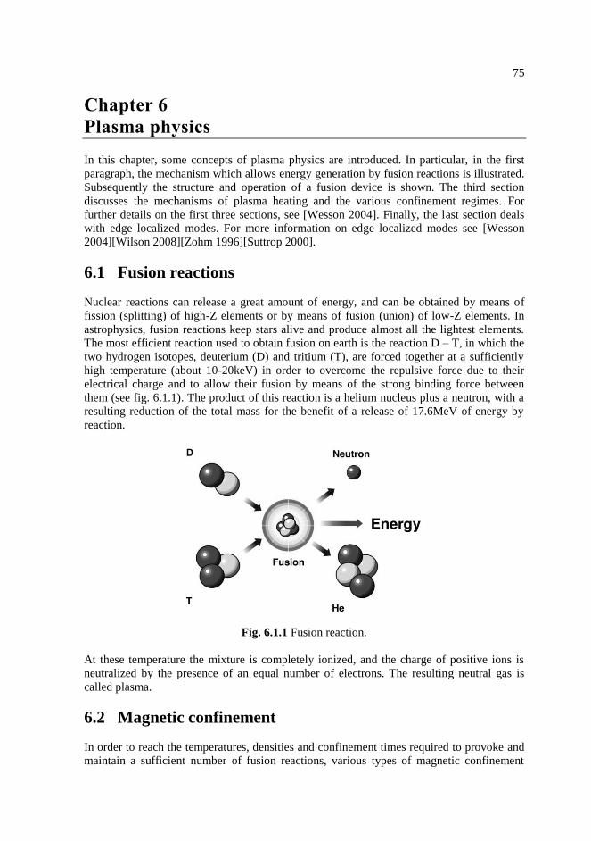
75
Chapter 6
Plasma physics
In this chapter, some concepts of plasma physics are introduced. In particular, in the first
paragraph, the mechanism which allows energy generation by fusion reactions is illustrated.
Subsequently the structure and operation of a fusion device is shown. The third section
discusses the mechanisms of plasma heating and the various confinement regimes. For
further details on the first three sections, see [Wesson 2004]. Finally, the last section deals
with edge localized modes. For more information on edge localized modes see [Wesson
2004][Wilson 2008][Zohm 1996][Suttrop 2000].
6.1 Fusion reactions
Nuclear reactions can release a great amount of energy, and can be obtained by means of
fission (splitting) of high-Z elements or by means of fusion (union) of low-Z elements. In
astrophysics, fusion reactions keep stars alive and produce almost all the lightest elements.
The most efficient reaction used to obtain fusion on earth is the reaction D – T, in which the
two hydrogen isotopes, deuterium (D) and tritium (T), are forced together at a sufficiently
high temperature (about 10-20keV) in order to overcome the repulsive force due to their
electrical charge and to allow their fusion by means of the strong binding force between
them (see fig. 6.1.1). The product of this reaction is a helium nucleus plus a neutron, with a
resulting reduction of the total mass for the benefit of a release of 17.6MeV of energy by
reaction.
Fig. 6.1.1 Fusion reaction.
At these temperature the mixture is completely ionized, and the charge of positive ions is
neutralized by the presence of an equal number of electrons. The resulting neutral gas is
called plasma.
6.2 Magnetic confinement
In order to reach the temperatures, densities and confinement times required to provoke and
maintain a sufficient number of fusion reactions, various types of magnetic confinement

76
devices have been designed. Among these, tokamak is the most highly developed
technology.
The tokamak is a toroidal plasma confinement system. This system consists essentially of a
toroidal ring surrounding a magnetic circuit, called core. Around the core, the coils and the
torus are wrapped. The central solenoid and the torus are respectively the primary and the
secondary circuit of a transformer. Current is supplied into the primary circuit (the central
solenoid), developing a magnetic induction flow in the magnetic circuit. If free electric
charges are present in the secondary circuit (the torus), they are accelerated and in the torus
an electric current is induced.
The principal magnetic field is the toroidal field, induced by the current flowing in the coils
wrapping around the torus along the poloidal direction. However, this field alone doesn’t
allow the plasma confinement. In order to have an equilibrium in which the plasma pressure
is balanced by the magnetic forces also a poloidal magnetic field is necessary. In a tokamak
this field is produced mainly by the plasma current flowing in the toroidal direction
according to Ampere’s law. The combination of the two magnetic fields give rise to
magnetic field lines with a helical trajectory around the torus.
The plasma is surrounded by a blanket, which has the role to absorb the neutrons,
transforming their energy into heat which is then carried away by a suitable coolant to
provide most of the reactor power output, to shield the superconducting coils and other outer
components and to allow the necessary breeding of tritium to fuel the reactor. The energy
flux of the neutrons which pass through the outer wall of the blanket must be reduced by a
factor 106 – 10
7 before reaching the superconducting coils to avoid both radiation damage
and heating of the coils. This protection is achieved by placing a shield of about 1m
thickness of high Z material such as steel between the blanket and the coils.
Additional coils are located externally for the plasma shape control.
In experimental tokamaks direct contact between the plasma and the first wall is avoided by
means of either a material limiter or by a divertor which leads magnetic field lines away
from the surface of the plasma to a dump plate more remote from the plasma.
Fig. 6.2.1 Magnetic confinement in a tokamak.

77
6.3 L-Mode and H-Mode
In an ignited D-T plasma the energy losses are balanced by the plasma heating from the
stowing down of the α-particles resulting from the fusion reactions. However, the fusion
reaction rate is a strong function of temperature and is negligible at low temperatures. Thus,
to reach the temperature required for ignition it is necessary to provide some form of
heating.
The initial heating in all tokamaks comes from the ohmic heating caused by the toroidal
current. At low temperatures ohmic heating is quite powerful and, in large tokamaks, easily
produces temperatures of a few keV. However, as the temperature increases, the collision
frequency and the resistivity fall, leading to the requirement for additional heating.
The two main methods designed for heating to ignition temperatures are the injection of
energetic neutral beams and the resonant absorption of radio frequency electromagnetic
waves.
The beams used for injection heating are composed of neutral particles. The choice of
neutral particles is due to the fact that the ions, positively charged particles, would be
reflected by the tokamak magnetic field. Heating with neutral beams is a complex process:
ions are produced and accelerated to the required energy and then neutralized by charge
exchange in a gas target; after removal of the residual ions, the neutral particles are injected
in the plasma where they are charged again, confined by the magnetic field and then slowed
by collisions giving up their energy in the process.
Radio frequency heating transfers energy from an external source to the plasma by means of
electromagnetic waves. There are several types of radio frequency heating, the three
principal ones involving waves at around the ion cyclotron frequency, the electron cyclotron
frequency and the lower hybrid frequency. When an electromagnetic wave propagates
through a plasma the electric field of the wave accelerates the charged particles which then
heat the plasma through collisions.
When the magnetically confined plasma is heated above a certain threshold level, it may
spontaneously switch from a low confinement state (or L-mode) to a high confinement state
(or H-mode). In the H-mode, the energy confinement time is significantly enhanced,
typically by a factor of two or greater than that in the standard L-mode discharges, leading
to edge pedestals in the temperature and density. A widely used scaling law for the
confinement time in H-mode can be found in [ITER 1999],
19.078.058.039.141.069.015.093.02,98 145.0 AaRnPBI eheattorp
yIPB
E (6.3.1)
where Ip is the plasma current in MA, Btor is the toroidal magnatic field in T, Pheat is the
auxiliary heating power in MW, ne is the line averaged electron density in 1020
m-3
, R is the
major radius in m, a is the minor radius in m, κ is the elongation and A is the mean atomic
mass.

78
6.4 Edge Localized Modes
In the H-mode, the pressure gradient on the plasma edge is typically high. While this is good
for confinement, instabilities called edge localized modes can be triggered.
Edge localized modes (ELMs) are repetitive bursts of the edge plasma. They can be
described by a cycle ([Wilson 2008]) divided into four phases:
Before the ELM the plasma is stable and has a high pressure gradient at the edge. The
gradient is maintained on a high level by the edge transport barrier, associated to the H-
mode, where the heat and particles transfer through the magnetic flux surfaces is
suppressed.
The pressure gradient overcomes the stability limit and many small turbulent eddies
appear at the edge.
The edge plasma is lost to the Scrape-Off Layer (SOL) where it flows along the
magnetic field lines towards the divertor.
The lost plasma ends up on the divertor plates producing the distinctive peak in the D-
alpha radiation (visible light emission by the excited atoms of deuterium, fig. 6.4.1). The
heat load produced by the ELMs on the divertor plates can cause erosion.
Fig. 6.4.1 Example of D-alpha emission during a Type-I ELM.
If the conditions remain stationary, the cycle can continue indefinitely. The ELM crash is
usually significantly shorter than the time between two ELMs. Depending on the type of
ELM and the state of the plasma, each ELM is able to remove from 1% to 7% of the plasma
energy and particles.
Over time, researchers ([Wilson 2008]) distinguished among different categories of ELMs,
each one characterized by specific properties. The first category is represented by Type-I
ELMs, also called large or even “giant” ELMs. During type-I ELMs, the plasma edge is
close to the theoretical stability limit or even beyond it, and the D-alpha radiation shows big
and isolated bursts. This kind of instability is guided by the pressure, and the ELM
frequency increases with the heating power.
The second category is represented by Type-II ELMs, also called grassy ELMs. Type-II
ELMs are observed only on high elongation, high triangularity and rather high density
plasmas. Their magnitude is lower and their frequency is greater than type-I ELMs.

79
The third and last category is represented by Type-III ELMs, also called small ELMs.
During type-III ELMs the D-alpha radiation shows small and frequent bursts. This kind of
instability is driven by electric current and appears when the plasma resistivity is rather high
(edge temperature rather low). The ELM frequency decreases with the heating power.
Between the different ELM types, during type-III ELMs the plasma confinement is
degraded more than with other ELMs.
In [Duro 2009] a method for the automated ELM classification has been addressed.
In the H-mode, paradoxically, ELMs contribute to maintain a stable plasma density. In fact,
in a H-mode without ELMs the plasma density would increase above the overall stability
limit, leading to sudden loss of the plasma confinement in a major instability called plasma
disruption. On the other hand, in order to decrease the divertor erosion and maintain a good
control on the pressure profile, several methods for the ELM mitigation has been
considered. The most promising approaches are the injection of small pellets of frozen fuel
into the plasma edge at a high frequency ([Lang 2004][Canik 2010]) and the ergodisation of
the plasma edge with magnetic field perturbations ([Bécoulet 2008]).
In [Zedda 2008], the results on the analysis of several ELM type-I time series suggest the
presence of deterministic chaos.


Part II.
Applications
…a light from the window, now I see …

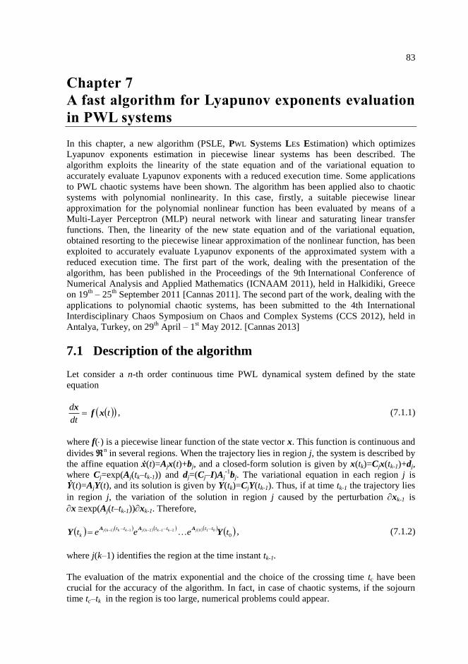
83
Chapter 7
A fast algorithm for Lyapunov exponents evaluation
in PWL systems
In this chapter, a new algorithm (PSLE, PWL Systems LEs Estimation) which optimizes
Lyapunov exponents estimation in piecewise linear systems has been described. The
algorithm exploits the linearity of the state equation and of the variational equation to
accurately evaluate Lyapunov exponents with a reduced execution time. Some applications
to PWL chaotic systems have been shown. The algorithm has been applied also to chaotic
systems with polynomial nonlinearity. In this case, firstly, a suitable piecewise linear
approximation for the polynomial nonlinear function has been evaluated by means of a
Multi-Layer Perceptron (MLP) neural network with linear and saturating linear transfer
functions. Then, the linearity of the new state equation and of the variational equation,
obtained resorting to the piecewise linear approximation of the nonlinear function, has been
exploited to accurately evaluate Lyapunov exponents of the approximated system with a
reduced execution time. The first part of the work, dealing with the presentation of the
algorithm, has been published in the Proceedings of the 9th International Conference of
Numerical Analysis and Applied Mathematics (ICNAAM 2011), held in Halkidiki, Greece
on 19th
– 25th
September 2011 [Cannas 2011]. The second part of the work, dealing with the
applications to polynomial chaotic systems, has been submitted to the 4th International
Interdisciplinary Chaos Symposium on Chaos and Complex Systems (CCS 2012), held in
Antalya, Turkey, on 29th
April – 1st May 2012. [Cannas 2013]
7.1 Description of the algorithm
Let consider a n-th order continuous time PWL dynamical system defined by the state
equation
tdt
dxf
x , (7.1.1)
where f() is a piecewise linear function of the state vector x. This function is continuous and
divides n in several regions. When the trajectory lies in region j, the system is described by
the affine equation ẋ(t)=Ajx(t)+bj, and a closed-form solution is given by x(tk)=Cjx(tk-1)+dj,
where Cj=exp(Aj(tk–tk-1)) and dj=(Cj–I)Aj-1
bj. The variational equation in each region j is
Ẏ(t)=AjY(t), and its solution is given by Y(tk)=CjY(tk-1). Thus, if at time tk-1 the trajectory lies
in region j, the variation of the solution in region j caused by the perturbation xk-1 is
xexp(Aj(t–tk-1))xk-1. Therefore,
001021211 teeet
tttttt
kjkkkjkkkj YY
AAA , (7.1.2)
where j(k–1) identifies the region at the time instant tk-1.
The evaluation of the matrix exponential and the choice of the crossing time tc have been
crucial for the accuracy of the algorithm. In fact, in case of chaotic systems, if the sojourn
time tc–tk in the region is too large, numerical problems could appear.
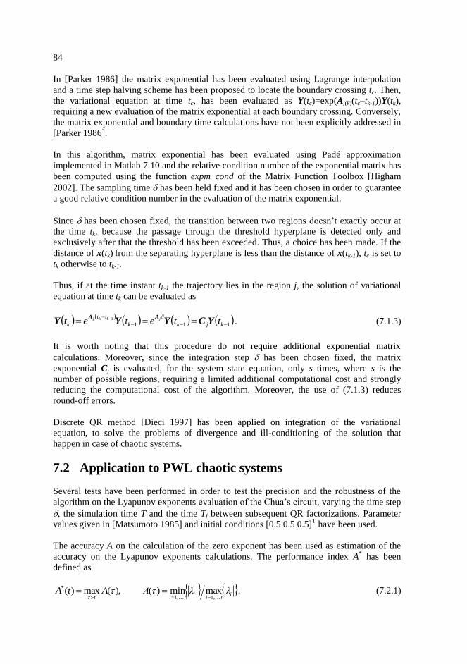
84
In [Parker 1986] the matrix exponential has been evaluated using Lagrange interpolation
and a time step halving scheme has been proposed to locate the boundary crossing tc. Then,
the variational equation at time tc, has been evaluated as Y(tc)=exp(Aj(k)(tc–tk-1))Y(tk),
requiring a new evaluation of the matrix exponential at each boundary crossing. Conversely,
the matrix exponential and boundary time calculations have not been explicitly addressed in
[Parker 1986].
In this algorithm, matrix exponential has been evaluated using Padé approximation
implemented in Matlab 7.10 and the relative condition number of the exponential matrix has
been computed using the function expm_cond of the Matrix Function Toolbox [Higham
2002]. The sampling time has been held fixed and it has been chosen in order to guarantee
a good relative condition number in the evaluation of the matrix exponential.
Since has been chosen fixed, the transition between two regions doesn’t exactly occur at
the time tk, because the passage through the threshold hyperplane is detected only and
exclusively after that the threshold has been exceeded. Thus, a choice has been made. If the
distance of x(tk) from the separating hyperplane is less than the distance of x(tk-1), tc is set to
tk otherwise to tk-1.
Thus, if at the time instant tk-1 the trajectory lies in the region j, the solution of variational
equation at time tk can be evaluated as
1111
kjkk
tt
k ttetet jkkj YCYYYAA
. (7.1.3)
It is worth noting that this procedure do not require additional exponential matrix
calculations. Moreover, since the integration step has been chosen fixed, the matrix
exponential Cj is evaluated, for the system state equation, only s times, where s is the
number of possible regions, requiring a limited additional computational cost and strongly
reducing the computational cost of the algorithm. Moreover, the use of (7.1.3) reduces
round-off errors.
Discrete QR method [Dieci 1997] has been applied on integration of the variational
equation, to solve the problems of divergence and ill-conditioning of the solution that
happen in case of chaotic systems.
7.2 Application to PWL chaotic systems
Several tests have been performed in order to test the precision and the robustness of the
algorithm on the Lyapunov exponents evaluation of the Chua’s circuit, varying the time step
, the simulation time T and the time Tf between subsequent QR factorizations. Parameter
values given in [Matsumoto 1985] and initial conditions [0.5 0.5 0.5]T have been used.
The accuracy A on the calculation of the zero exponent has been used as estimation of the
accuracy on the Lyapunov exponents calculations. The performance index A* has been
defined as
i, . . .ni
i,. . .nit
λλΑAtA11
* maxmin)(),(max)(
. (7.2.1)

85
The accuracy A(t) oscillates during the Lyapunov exponents estimation. Thus, it is strongly
dependent on the time instant t. Conversely, A*(t)
is monotonically decreasing. The index
A*(t), which can be only calculated at the end of the Lyapunov exponents evaluation, is
representative of the worst value assumed by the accuracy after t. In this sense it is a
measure of the improvement on the accuracy during the Lyapunov exponents estimation
procedure.
Fig. 7.2.1 A
* during the calculation of the zero exponent with respect to (a) simulation time
(b) calculation time.
Fig. 7.2.1 reports a measure of the accuracy A* with respect to simulation time and
calculation time for different values of and Tf. In order to evaluate A* the simulation has
been stopped after 10000s even if the Lyapunov exponents calculation is reported for 5000s.
Fig. 7.2.1(a) reports A* with respect to the simulation time. As it can be noticed, PSLE is not
particularly affected by the QR factorization frequency. This parameter is generally critical
for the accuracy of Lyapunov exponents. Smaller values generally lead to more accurate
results, but take longer time, since the numerical integration needs to be restarted many
100
101
102
103
10-3
10-2
10-1
simulation time (s)
pre
cisi
on
A*
=5ms Tf=50ms
=5ms Tf=100ms
=5ms Tf=250ms
=10ms Tf=100ms
=10ms Tf=200ms
=10ms Tf=500ms
=20ms Tf=200ms
=20ms Tf=400ms
=20ms Tf=1000ms
a)
0.01" 0.1" 1" 10" 20"
10-3
10-2
10-1
computation time
pre
cisi
on
A*
=5ms Tf=50ms
=5ms Tf=100ms
=5ms Tf=250ms
=10ms Tf=100ms
=10ms Tf=200ms
=10ms Tf=500ms
=20ms Tf=200ms
=20ms Tf=400ms
=20ms Tf=1000ms
b)

86
times for short calculations. PSLE is robust with respect to the different time steps: the
largest one, = 20ms, seems to show the more fast convergence. Nevertheless, for t>2000s,
when Lyapunov exponents settle to approximately their asymptotic value, best performance
have been obtained with = 5ms.
Fig. 7.2.1(b) reports the performance versus the calculation time. For a given calculation
time, best performance have been obtained when = 20ms irrespective of Tf. Thus, fixing
the calculation time, the test with the highest time step, i.e., longer simulations, shows the
best values of precision.
PSLE has been compared to LET [LET] and PWL algorithm in [Chialina 1994]. The
algorithm in LET is an integration of the two algorithms in [Eckmann 1985], [Wolf 1985].
The graphical interface has been disabled since it causes a growth of calculation time. The
same algorithms ([Eckmann 1985], [Wolf 1985]) are also implemented in MATDS and
Mathematica.
In tables 7.2.1 and 7.2.2 the parameters values for the different tests and the obtained values
of Lyapunov exponents, precision and calculation time respectively, have been reported.
Since LET performance and calculation time depend on Tf, Lyapunov exponents have been
evaluated for three values of Tf. Conversely, since PSLE is not influenced by Tf (see
Fig.7.2.1a) only one value of Tf has been tested.
Table 7.2.1 Parameter values for the LEs calculation.
PSLE LET [Chialina 1994]
Step Fixed Variable N. A.
[ms] 5 - N.A.
ODE solver Matrix exponential Runge-Kutta Matrix exponential
Tf [ms] 100 100, 200, 500 N.A.
T [s] 5000 5000 5000
Table 7.2.2 Comparison of the performance.
PSLE
LET [Chialina 1994]
tf =100ms tf = 200ms tf = 500ms
Lyapunov
exponents
0.2329
-0.0009
-1.7771
0.2378
0.0007
-1.7906
0.2379
-0.0028
-1.7488
0.2287
-0.0003
-1.7845
0.23
0.00
-1.78
A*(T) 9.182 10-4 8.062 10-4 2.269 10-3 1.461 10-3 -
Tc 17” 26’ 32’’ 13’ 52’’ 5’ 46’’ N.A.
The accuracy of PSLE is slightly better if compared with that obtained in [Chialina 1994]
using an extrapolation filter to accelerate the convergence. The calculation time is
significantly shortened. LET reaches better values of A* when Tf = 100ms, at expense of a
huge calculation time. For other Tf values, LET performance is worst and PSLE results more
than an order of magnitude fast. Moreover, the time requested by LET and PSLE in order to
achieve the same accuracy has been evaluated. Varying Tf, LET employs 11’ 41’’, 27’ 43’’,
29’ 59’’, to achieve 9.182 10-4
versus 17’’ spent by the algorithm. PSLE employs 57” to
achieve the best value of accuracy, A*=8.062e-4, reached by LET in 26’ 32’’. Thus, PSLE
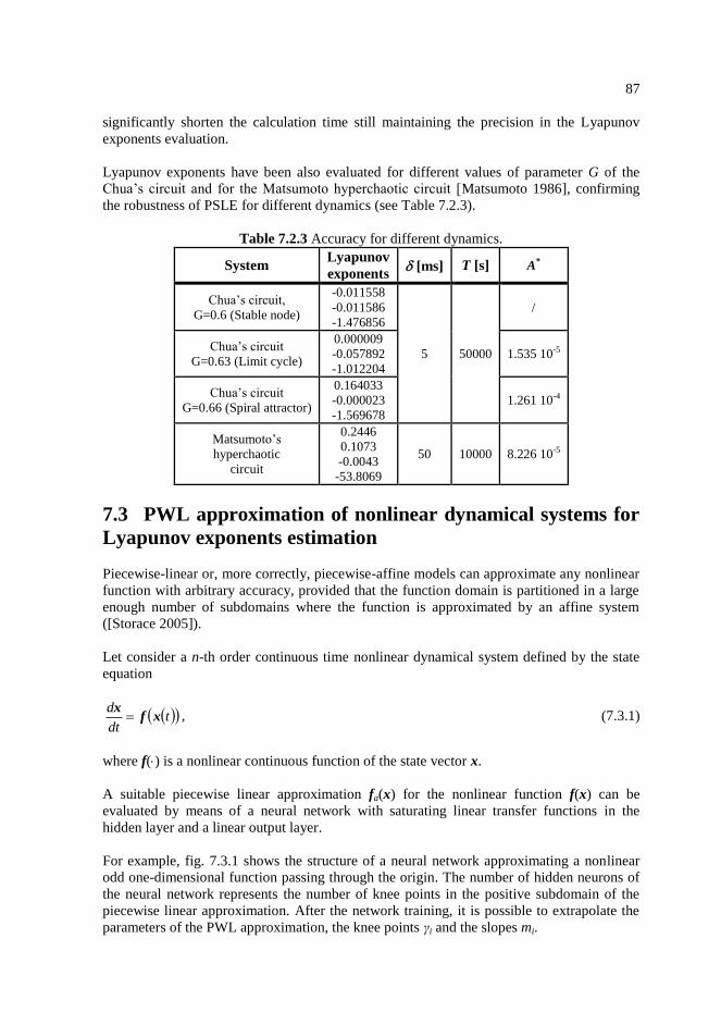
87
significantly shorten the calculation time still maintaining the precision in the Lyapunov
exponents evaluation.
Lyapunov exponents have been also evaluated for different values of parameter G of the
Chua’s circuit and for the Matsumoto hyperchaotic circuit [Matsumoto 1986], confirming
the robustness of PSLE for different dynamics (see Table 7.2.3).
Table 7.2.3 Accuracy for different dynamics.
System Lyapunov
exponents [ms] T [s] A*
Chua’s circuit,
G=0.6 (Stable node)
-0.011558
-0.011586
-1.476856
5 50000
/
Chua’s circuit
G=0.63 (Limit cycle)
0.000009
-0.057892
-1.012204
1.535 10-5
Chua’s circuit
G=0.66 (Spiral attractor)
0.164033
-0.000023
-1.569678
1.261 10-4
Matsumoto’s
hyperchaotic
circuit
0.2446
0.1073
-0.0043
-53.8069
50 10000 8.226 10-5
7.3 PWL approximation of nonlinear dynamical systems for
Lyapunov exponents estimation
Piecewise-linear or, more correctly, piecewise-affine models can approximate any nonlinear
function with arbitrary accuracy, provided that the function domain is partitioned in a large
enough number of subdomains where the function is approximated by an affine system
([Storace 2005]).
Let consider a n-th order continuous time nonlinear dynamical system defined by the state
equation
tdt
dxf
x , (7.3.1)
where f() is a nonlinear continuous function of the state vector x.
A suitable piecewise linear approximation fa(x) for the nonlinear function f(x) can be
evaluated by means of a neural network with saturating linear transfer functions in the
hidden layer and a linear output layer.
For example, fig. 7.3.1 shows the structure of a neural network approximating a nonlinear
odd one-dimensional function passing through the origin. The number of hidden neurons of
the neural network represents the number of knee points in the positive subdomain of the
piecewise linear approximation. After the network training, it is possible to extrapolate the
parameters of the PWL approximation, the knee points γi and the slopes mi.
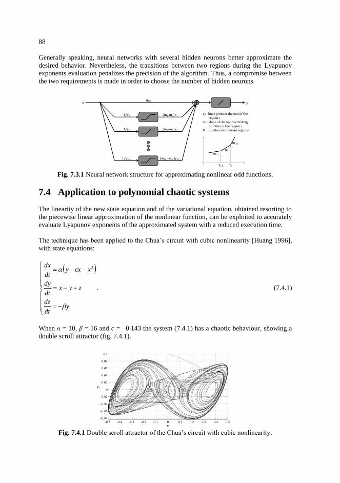
88
Generally speaking, neural networks with several hidden neurons better approximate the
desired behavior. Nevertheless, the transitions between two regions during the Lyapunov
exponents evaluation penalizes the precision of the algorithm. Thus, a compromise between
the two requirements is made in order to choose the number of hidden neurons.
Fig. 7.3.1 Neural network structure for approximating nonlinear odd functions.
7.4 Application to polynomial chaotic systems
The linearity of the new state equation and of the variational equation, obtained resorting to
the piecewise linear approximation of the nonlinear function, can be exploited to accurately
evaluate Lyapunov exponents of the approximated system with a reduced execution time.
The technique has been applied to the Chua’s circuit with cubic nonlinearity [Huang 1996],
with state equations:
ydt
dz
zyxdt
dy
xcxydt
dx
3
. (7.4.1)
When α = 10, β = 16 and c = –0.143 the system (7.4.1) has a chaotic behaviour, showing a
double scroll attractor (fig. 7.4.1).
Fig. 7.4.1 Double scroll attractor of the Chua’s circuit with cubic nonlinearity.

89
The cubic non linearity f(x) = x3 has been approximated with a PWL function fa(x), using the
neural network shown in fig. 7.3.1. Table 7.4.1 shows the mean squared error between f(x)
and the PWL approximation fa(x), varying the number of regions M in the positive
subdomain.
Table 7.4.1 Mean squared error (MSE) on approximation of the cubic nonlinearity varying
the number of regions.
N° of regions 2 3 4 5 6
MSE 1.442∙10-5
2.378∙10-6
7.592∙10-7
2.822∙10-7
1.324∙10-7
N° of regions 7 8 9 10 11
MSE 6.881∙10-8
4.061∙10-8
2.547∙10-8
1.631∙10-8
1.113∙10-8
N° of regions 12 13 14 15 16
MSE 7.627∙10-9
5.786∙10-9
4.210∙10-9
3.357∙10-9
2.675∙10-9
For each value of M, the approximated PWL system
ydt
dz
zyxdt
dy
xfcxydt
dxa
(7.4.2)
has been integrated. Fig. 7.4.2 shows the attractors corresponding to the values M = 2, 4, 8
and 16.
Fig. 7.4.2 Attractors corresponding to the values of
(a) M = 2, (b) M = 4, (c) M = 8 and (d) M = 16.
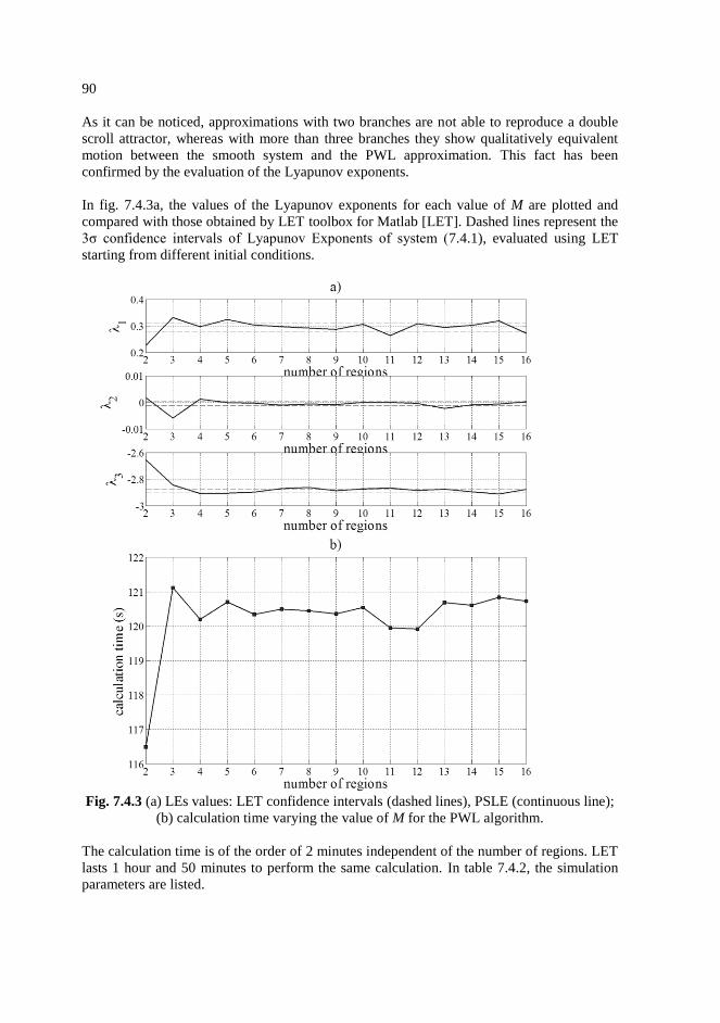
90
As it can be noticed, approximations with two branches are not able to reproduce a double
scroll attractor, whereas with more than three branches they show qualitatively equivalent
motion between the smooth system and the PWL approximation. This fact has been
confirmed by the evaluation of the Lyapunov exponents.
In fig. 7.4.3a, the values of the Lyapunov exponents for each value of M are plotted and
compared with those obtained by LET toolbox for Matlab [LET]. Dashed lines represent the
3σ confidence intervals of Lyapunov Exponents of system (7.4.1), evaluated using LET
starting from different initial conditions.
Fig. 7.4.3 (a) LEs values: LET confidence intervals (dashed lines), PSLE (continuous line);
(b) calculation time varying the value of M for the PWL algorithm.
The calculation time is of the order of 2 minutes independent of the number of regions. LET
lasts 1 hour and 50 minutes to perform the same calculation. In table 7.4.2, the simulation
parameters are listed.

91
Table 7.4.2 Parameter values for Lyapunov exponents estimation.
Time step N° iterations Initial conditions
5ms 2∙106 [0 0 0.1]
7.5 Conclusions
PSLE, an algorithm for Lyapunov exponents evaluation in PWL systems, has been
proposed. The algorithm solves in closed form the state and the variational equations taking
into account the issues of crossing time and the matrix exponential estimations. The
computational cost is considerably reduced without compromising the precision. Results
have been compared with those obtained by algorithms presented in literature for PWL
systems and by the LET toolbox without graphical interface, demonstrating the
effectiveness of the approach.
The algorithm has been extended to non linear systems with polynomial nonlinearity, by
means of a PWL approximation of the nonlinear function. The suitable approximation is
evaluated by means of a Multi-Layer Perceptron with linear and saturating linear transfer
functions. PSLE is then applied to a new system with the piecewise linear approximation of
the nonlinear function. Comparisons with results obtained by LET with disabled graphical
interface have been reported in the case of Lyapunov exponents evaluation for the Chua’s
circuit. Results confirm that the proposed algorithm allows one a fast evaluation of
Lyapunov exponents without compromising the accuracy of the calculation.


93
Chapter 8
Effect of a particular coupling on the dynamic
behavior of nonlinear systems
In this chapter, a systematic method to project systems of order 2n characterized by two
positive Lyapunov exponents, is proposed. This procedure couples nth-order chaotic
systems with a suitable non linear coupling function. Examples of polynomial and piecewise
linear systems have been proposed. Both numerical simulation and circuit implementation
have been performed. Transformation techniques have been applied to the study of these
systems; in particular, the analysis of the transverse and tangent systems has shown that they
are equivalent to two uncoupled identical chaotic systems of order three. The work has been
published in the International Journal of Circuit Systems and Applications.
8.1 General approach
Let us consider a system described by
)(xfAxx
dt
d, (8.1.1)
where x = (x1 x2 … xn)T Rn
and f (x) =(f1(x) f2(x) … fn(x))T is a nonlinear function on Rn
.
The coupling functions g and h are introduced to couple two identical systems of the form
(8.1.1) obtaining
),()(
),()(
21222
21111
xxgxfAxx
xxhxfAxx
dt
d
dt
d
S (8.1.2)
The transverse and tangent systems are
),(),()()(
),(),()()(
212121||
||
212121
xxgxxhxfxfAxx
xxgxxhxfxfAxx
dt
d
dt
d
. (8.1.3)
If
)(),(),()()(
)(),(),()()(
21212121
21212121
xxfxxgxxhxfxf
xxfxxgxxhxfxf, (8.1.4)
i.e.,

94
)(5.0)(5.0)()(
)(5.0)(5.0)()(
212121
212112
xxfxxfxfxg
xxfxxfxfxh (8.1.5)
system (8.1.3) becomes
)(
)(
||||
||xfAx
x
xfAxx
dt
d
dt
d
, (8.1.6)
with
20100||
20100
xxx
xxx. (8.1.7)
In this case, transverse and tangent systems are two uncoupled systems, identical to the
original systems. The effect of the coupling is the same effect of a change in the initial
conditions x10 and x20 of the uncoupled systems. Thus, if the initial conditions of S// are in
the same basin of attraction of [x10 x20] the S// dynamics is the same of system S.
The linear transformation of the state variables leads to the uncoupling of the equations
governing the behavior of the 6th
order system by splitting the state space in subspaces. As it
can be noticed, the two systems S and S// are two identical uncoupled systems.
System S and system S// composed by S// and S are equivalent under a linear
transformation of the state variables. Since LEs are invariant under linear transformations of
the state variables, S and S// are characterized by the same LEs.
If system S is chaotic, system S//, being composed of two chaotic systems, is characterized
by two identical positive LEs. For this reason, system S too presents two positive LEs.
However, its dynamics is equivalent to that of system S//, i.e., to that of two uncoupled
systems in chaotic regime, S// and S. Thus, although system S has two positive LEs, it can
be considered hyperchaotic at the same level as any other pair of uncoupled chaotic systems.
8.2 Application to PWL chaotic systems
Let us consider the Chua’s circuit with PWL nonlinearity. System equations are
11
1
2
1
2
1
2
1
1
11
1
1
1
1
1
1
yLdt
dz
zC
yC
Gx
C
G
dt
dy
C
xfy
C
Gx
C
G
dt
dx
, (8.2.1)

95
where
ExExGGxGxf bab 111 5.0)( . (8.2.2)
If C1 = 10nF, C2 = 100nF, L = 18mH, R1 = 6.6kΩ, R2 = R3 = 44kΩ, R4 = 4.4kΩ, R5 = R6 =
440Ω, G = 1/1670Ω-1
the system shows a chaotic behavior and it is characterized by one
positive, one negative and one null LE.
The Chua’s circuit is characterized by three fixed points
EG
GG
GGE
GG
GGPEG
GG
GGE
GG
GG=PP
b
ab
b
ba
b
ba
b
ab ,0,,0,0,0,0 210 , (8.2.3)
which, in chaotic regime, are non-stable. The origin is a saddle point for all values of the
parameters.
Let us consider two identical Chua’s circuits S1 and S2. The dynamics of the system S,
obtained bidirectionally coupling S1 and S2, is described by a set of six differential
equations, i.e.,
22
2
2
2
2
2
2
2
2121
1
2
1
2
1
2
11
1
2
1
2
1
2
1
2121
1
1
1
1
1
1
1
1
2
1
1
1
2
1
yLdt
dz
zC
yC
Gx
C
G
dt
dy
xxfxxfC
yC
Gx
C
G
dt
dx
yLdt
dz
zC
yC
Gx
C
G
dt
dy
xxfxxfC
yC
Gx
C
G
dt
dx
S , (8.2.4)
where
2121
1
1
1
212
1)(
1),( xxfxxf
Cxf
Cxxh (8.2.5)
2121
1
2
1
212
1)(
1),( xxfxxf
Cxf
Cxxg (8.2.6)
The analogue circuit representing system S is shown in fig. 8.2.1.

96
As it can be noticed when x2=0 (x1=0), the left (right) part of the circuit is an independent
Chua’s circuit.
The system S is characterized by six Lyapunov exponents and one or two Lyapunov
exponents could be positive. In this case, the parameters are chosen to obtain that each
Chua’s circuit subsystem operates in the chaotic regime.
Fig. 8.2.1 6
th order circuit with PWL nonlinearity.
In order to simplify the analysis of the dynamical behaviour of the system, let us introduce
the transverse systems S and the tangent system S//. The transverse and tangent systems are
respectively defined by the state variables
21
21
21
zzz
yyy
xxx
21
21
21
zzz
yyy
xxx
//
//
//
. (8.2.7)
A direct substitution of (8.2.7) into (8.2.4) leads to the new state equations
97
yLdt
dz
zC
yC
Gx
C
G
dt
dy
xgC
yC
Gx
C
G
dt
dx
S
1
1
1
222
111
(8.2.8)
//
//
2
//
2
//
2
//
1
//
1
//
1
//
//
1
1
1
yLdt
dz
zC
yC
Gx
C
G
dt
dy
xgC
yC
Gx
C
G
dt
dx
S . (8.2.9)
The linear transformation of the state variables leads to the uncoupling of the equations
governing the behavior of the 6th
order system by splitting the state space in subspaces. As it
can be noticed, the two systems S and S// are two identical uncoupled Chua’s circuits.
System S and system S// composed by S// and S are equivalent under a linear
transformation of the state variables. Since LEs are invariant under linear transformations of
the state variables, S and S// are characterized by the same LEs.
System S//, being composed of two Chua’s circuits, is characterized by two identical
positive LEs. For this reason, system S too presents two positive LEs. However, its
dynamics is equivalent to that of system S//, i.e., to that of two uncoupled Chua’s systems in
chaotic regime, S// and S. Thus, system S can be considered hyperchaotic at the same level
as any other pair of uncoupled chaotic systems.
If the initial point of S or S// is not one of the fixed points P1,2 in (8.2.3), also the
generalised synchronization
EGGG
GGzz
yy
EGG
GGxx
b
ba
b
ab
21
21
21
0 (8.2.10)
can be excluded.
8.2.1. Numerical results
The system equations have been solved using Matlab. The integration method was Runge
Kutta with time step equal to 10-6
. Typical hyperchaotic attractors shown in fig. 8.2.2 have
been obtained.
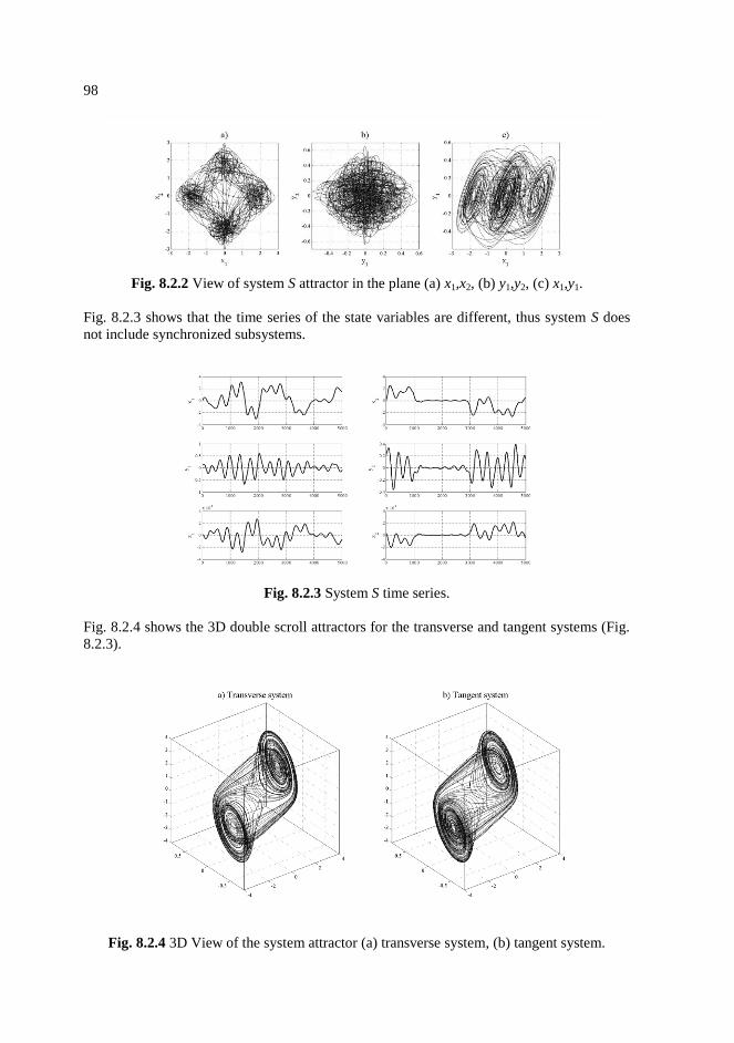
98
Fig. 8.2.2 View of system S attractor in the plane (a) x1,x2, (b) y1,y2, (c) x1,y1.
Fig. 8.2.3 shows that the time series of the state variables are different, thus system S does
not include synchronized subsystems.
Fig. 8.2.3 System S time series.
Fig. 8.2.4 shows the 3D double scroll attractors for the transverse and tangent systems (Fig.
8.2.3).
Fig. 8.2.4 3D View of the system attractor (a) transverse system, (b) tangent system.

99
8.2.2. Experimental results
To verify the practical feasibility of the circuit, it has been realized in laboratory using
standard components. The operational amplifiers are TL082 powered by 9V batteries, G is a
potentiometer of 2k, the resistors are 1/4W with 5% tolerance, the inductor has been
realized with an active circuit [19].
Fig. 8.2.5 shows a 2D projection of the double scroll attractor obtained imposing x2=0.
Fig. 8.2.6 shows the voltage x1 of the capacitor C1 vs. the voltage y1 of the capacitor C2 (fig.
8.2.6a), the 2D attractor obtained measuring the voltages x1 and x2 of the capacitors C1 (fig.
8.2.6b) and the voltages y1 and y2 of the capacitors C2 (fig. 8.2.6c).
Fig. 8.2.5 2D View of the Chua’s circuit attractor obtained imposing x2=0.
Fig. 8.2.6 2D View of the 6D-system attractor on the plane (a) x1,y1, (b) x1,x2, (c) y1,y2.
Fig. 8.2.7 shows the 3D views of tangent and transverse systems attractors obtained by
processing the experimental data with Matlab.

100
Fig. 8.2.7 2D View of the experimental system attractor (a) transverse system, (b) tangent
system.
As it can be noticed, comparing the attractors in fig. 8.2.2 and 8.2.6 and those in fig. 8.2.4
and 8.2.7, experimental results are in agreement with numerical simulations.
Lyapunov exponents of system S have been evaluated starting from the experimental time
series using TISEAN [20]. The LEs spectra estimated from a time series of 10000 samples
is [5669 2202 146 -1293 -4369 -11589], where the third one can be considered as null when
compared with the other values. Moreover, the effect of component tolerances results in the
difference between the Lyapunov exponents of the uncoupled Chua’s circuits and those of
system S. In particular, one of the two null Lyapunov exponents becomes less than zero in
system S.
8.3 Application to polynomial chaotic systems
Let us consider the Chua’s circuit with cubic nonlinearity. System equations are the same in
(8.2.1) and
3
31 xxxf (8.3.1)
If = 10, = 16, c = 0.143 the system shows a chaotic behavior and it is characterized by
one positive, one negative and one null Lyapunov exponent.
Three equilibrium points exist, i.e.
ccPcc=PP ,0,,0,0,0,0 210 , (8.3.2)
and, in chaotic regime, the three equilibrium points are non-stable.
Let us consider two identical Chua’s circuits S1 and S2. The dynamics of the system S,
shown in fig. 8.3.1, obtained bidirectionally coupling S1 and S2, is described by a set of six
differential equations, i.e.,

101
Fig. 8.3.1 6
th order circuit with polynomial non linearity.
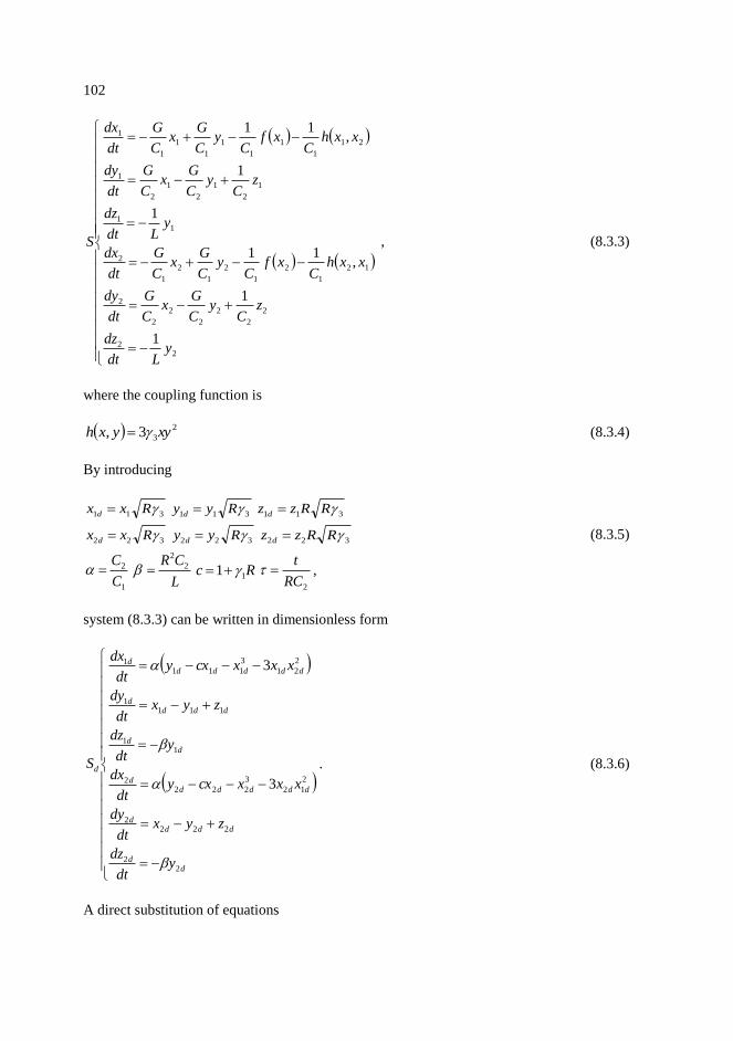
102
22
2
2
2
2
2
2
2
12
1
2
1
2
1
2
1
2
11
1
2
1
2
1
2
1
21
1
1
1
1
1
1
1
1
1
1
,11
1
1
,11
yLdt
dz
zC
yC
Gx
C
G
dt
dy
xxhC
xfC
yC
Gx
C
G
dt
dx
yLdt
dz
zC
yC
Gx
C
G
dt
dy
xxhC
xfC
yC
Gx
C
G
dt
dx
S , (8.3.3)
where the coupling function is
2
33, xyyxh (8.3.4)
By introducing
311 Rxx d 311 Ryy d 311 RRzz d
322 Rxx d 322 Ryy d 322 RRzz d (8.3.5)
1
2
C
C
L
CR 2
2
Rc 11 2RC
t ,
system (8.3.3) can be written in dimensionless form
dd
dddd
dddddd
dd
dddd
dddddd
d
ydt
dz
zyxdt
dy
xxxcxydt
dx
ydt
dz
zyxdt
dy
xxxcxydt
dx
S
22
2222
2
12
3
2222
11
1111
2
21
3
1111
3
3
. (8.3.6)
A direct substitution of equations

103
ddd
ddd
ddd
zzz
yyy
xxx
21
21
21
dd//d
dd//d
dd//d
zzz
yyy
xxx
21
21
21
(8.3.7)
into (8.3.6) leads to the state equations for the transverse and tangent systems
dd
dddd
ddddddddd
d
yd
dz
zyxd
dy
xxxxxxcxyd
dx
S
3 2
12
2
21
3
2
3
1
, (8.3.8)
dd
dddd
ddddddddd
d
yd
dz
zyxd
dy
xxxxxxcxyd
dx
S
////
////////
2
12
2
21
3
2
3
1//////
//
3
, (8.3.9)
i.e.,
dd
dddd
dddd
d
yd
dz
zyxd
dy
xcxyd
dx
S
3
, (8.3.10)
dd
dddd
dddd
d
yd
dz
zyxd
dy
xcxyd
dx
S
////
////////
3
||||////
//
. (8.3.11)
The systems Sd and S//d are two Chua’s circuits with cubic non linearity. Thus, system Sd,
obtained coupling two Chua’s circuits through a polynomial nonlinear function, is
equivalent to system S//d consisting of the same but uncoupled Chua’s circuits. The initial
conditions of S//d can be obtained substituting in (8.3.7) the initial conditions of Sd. Thus,
the only effect of the coupling function on Sd dynamics is a change in the initial conditions
of the original uncoupled circuits.
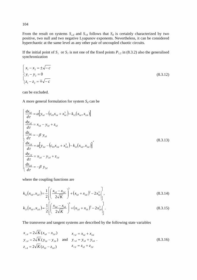
104
From the result on systems Sd and S//d follows that Sd is certainly characterized by two
positive, two null and two negative Lyapunov exponents. Nevertheless, it can be considered
hyperchaotic at the same level as any other pair of uncoupled chaotic circuits.
If the initial point of S or S// is not one of the fixed points P1,2 in (8.3.2) also the generalised
synchronization
czz
yy
cxx
21
21
21
0 (8.3.12)
can be excluded.
A more general formulation for system Sd can be
dd
dddd
dddddd
dd
dddd
dddddd
yd
dz
zyxd
dy
xxkxxcyd
dx
yd
dz
zyxd
dy
xxkxxcyd
dx
22
2222
2121
3
220322
11
1111
2112
3
110311
,
,
, (8.3.13)
where the coupling functions are
3
1
3
21
3
212112 2
22
1, ddd
dddd xxx
K
xxxxk , (8.3.14)
3
2
3
12
3
122121 2
22
1, ddd
dddd xxx
K
xxxxk . (8.3.15)
The transverse and tangent systems are described by the following state variables
)(2
)(2
)(2
21
21
21
ddd
ddd
ddd
zzKz
yyKy
xxKx
and
ddd
ddd
ddd
zzz
yyy
xxx
21//
21//
21//
. (8.3.16)

105
The transverse and tangent system equations show that they are still two uncoupled Chua’s
circuits. The parameter K does not appear in their state equations. Thus, the number of
positive Lyapunov exponents does not depend on the value of K. If K = 1/4 is assumed.
there is a large simplification in the coupling function expressions. In this case
2
212112 3, dddd xxxxk , (8.3.17)
2
122121 3, dddd xxxxk , (8.3.18)
and system (8.3.13) turns to system (8.3.6).
8.3.1. Numerical results
The system Sd is characterized by six Lyapunov exponents. If = 10, = 16, c = 0.143, Sd
has two positive, two negative and two null Lyapunov exponents. The system equations
have been simulated using Matlab. The integration method was Runge Kutta with fixed time
step equal to 6·10-3
.
Under the initial conditions [0, 0.15, 3·10-4
, 0, 0.05, 10-4
], the attractors shown in fig. 8.3.2
have been obtained.
Fig. 8.3.2 View of the Sd attractor in the plane (a) x1d,x2d, (b) y1d,y2d.
Fig. 8.3.3 shows that the time series of the state variables are different, thus Sd does not
include synchronized subsystems. The presence of two positive Lyapunov exponents and
the absence of synchronization would lead to the hypothesis of hyperchaotic behavior.
8.4 Conclusions
Generally speaking, depending on the coupling function, the qualitative behaviour of two
coupled systems, could be different by the one of the uncoupled systems.
A systematic method to project systems of order 2n characterized by two positive Lyapunov
exponents, has been proposed. The procedure couples nth-order chaotic systems with a
suitable non linear coupling function.

106
Fig. 8.3.3 System Sd time series.
In particular, this study focused on particular sixth-order dynamic systems characterized by
two positive Lyapunov exponents, occurrence generally assumed as a signature of
hyperchaos. The dynamic behavior of these systems has been investigated applying
transformation techniques, i.e., analyzing transverse and tangent 3-D systems. The analysis
of the transverse and tangent systems showed that they are equivalent to two uncoupled
identical chaotic systems of order three. Examples of polynomial and piecewise linear
systems are proposed. Both numerical simulation and circuit implementation have been
performed.
The presence of two positive Lyapunov exponents is generally considered a signature of
hyperchaos. This analysis suggests some considerations about the hyperchaoticity of these
systems. Indeed, despite the presence of two Lyapunov exponents, these systems can be
considered hyperchaotic at the same level as any other pair of uncoupled chaotic circuits.

107
Chapter 9
Identification of parameters in nonlinear dynamical
systems by neural networks
In this chapter a traditional Multi Layer Perceptron with a tapped delay line as input has
been trained to identify the parameters of the Chua’s circuit when fed with a sequence of
values of a scalar state variable. The analysis of the a priori identifiability of the system,
performed resorting to differential algebra, has allowed to choose a suitable observable and
the minimum number of taps. The results has confirmed the appropriateness of the proposed
approach. The work has been submitted to the 4th International Interdisciplinary Chaos
Symposium on Chaos and Complex Systems (CCS 2012), held in Antalya, Turkey, on 29th
April -1st May 2012.
9.1 General approach
Let us consider a time-invariant, nonlinear system described by the model:
]),([ ,,),,( uthyutdt
dxppxf
x (9.1.1)
where f and h are algebraic functions in x, p is a P-dimensional parameter vector, u is the
system input and y is a scalar output.
The main purpose is to identify the system parameters in (9.1.1) by means of the observable
y, after that their identifiability has been verified by means of the differential algebra
approach. The relationship between parameters and the observable is then captured by the
training of a neural network with memory. The network input consists of sequences of the
observable variables and the network outputs are the system parameters.
The solution of the identifiability problem, when it exists, allows one to identify the state
variable necessary to identify the unknown parameters and it determines the neural network
architecture.
9.2 Application to the Chua’s circuit with cubic nonlinearity
The Chua’s circuit with a polynomial nonlinearity has been considered [21], with equations
23
3212
3
111
xdt
dx
xxxdt
dx
xcxydt
dx
(9.2.1)
The input output relationship (IOR) corresponding to the output y = x1 is
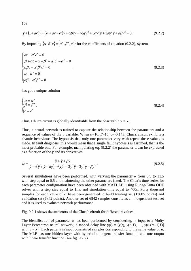
108
03361 3222 yyyyyyycyycycy . (9.2.2)
By imposing cc ,,,, for the coefficients of equation (9.2.2), system
0
0
0
0
0
cc
cc
cc
, (9.2.3)
has got a unique solution
cc
. (9.2.4)
Thus, Chua's circuit is globally identifiable from the observable y = x1.
Thus, a neural network is trained to capture the relationship between the parameters and a
sequence of values of the y variable. When α=10, β=16, c=-0.143, Chua's circuit exhibits a
chaotic behaviour. The hypotesis that only one parameter vary with repect these values is
made. In fault diagnosis, this would mean that a single fault hypotesis is assumed, that is the
most probable one. For example, manipulating eq. (9.2.2) the parameter α can be expressed
as a function of the y and its derivatives
3222 336 yyyyyyyyyycy
yyy
. (9.2.5)
Several simulations have been performed, with varying the parameter α from 8.5 to 11.5
with step equal to 0.5 and maintening the other parameters fixed. The Chua’s time series for
each parameter configuration have been obtained with MATLAB, using Runge-Kutta ODE
solver with a step size equal to 1ms and simulation time equal to 400s. Forty thousand
samples for each value of have been generated to build training set (13685 points) and
validation set (6842 points). Another set of 6842 samples constitutes an independent test set
and it is used to evaluate network performance.
Fig. 9.2.1 shows the attractors of the Chua’s circuit for different α values.
The identification of parameter α has been performed by considering, in input to a Multy
Layer Perceptron neural network, a tapped delay line y(t) = [y(t), y(t–T), …, y(t–(m–1)T)]
with y = x1. Each pattern in input consists of samples corresponding to the same value of α.
The MLP has one hidden layer with hyperbolic tangent transfer function and one output
with linear transfer function (see fig. 9.2.2).
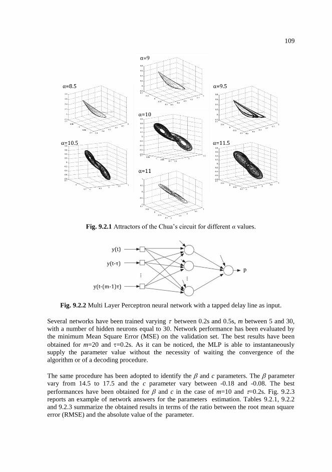
109
Fig. 9.2.1 Attractors of the Chua’s circuit for different α values.
Fig. 9.2.2 Multi Layer Perceptron neural network with a tapped delay line as input.
Several networks have been trained varying between 0.2s and 0.5s, m between 5 and 30,
with a number of hidden neurons equal to 30. Network performance has been evaluated by
the minimum Mean Square Error (MSE) on the validation set. The best results have been
obtained for m=20 and =0.2s. As it can be noticed, the MLP is able to instantaneously
supply the parameter value without the necessity of waiting the convergence of the
algorithm or of a decoding procedure.
The same procedure has been adopted to identify the and c parameters. The parameter
vary from 14.5 to 17.5 and the c parameter vary between -0.18 and -0.08. The best
performances have been obtained for and c in the case of m=10 and =0.2s. Fig. 9.2.3
reports an example of network answers for the parameters estimation. Tables 9.2.1, 9.2.2
and 9.2.3 summarize the obtained results in terms of the ratio between the root mean square
error (RMSE) and the absolute value of the parameter.

110
a)
b)
c)
Fig. 9.2.3 Target (continuous line) and network output (dots) fora parameter, (b)
parameter, (c) c parameter.
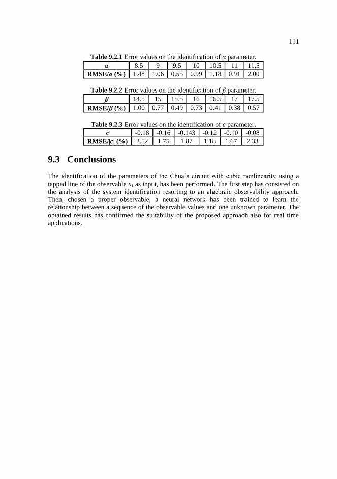
111
Table 9.2.1 Error values on the identification of α parameter.
α 8.5 9 9.5 10 10.5 11 11.5 RMSE/α (%) 1.48 1.06 0.55 0.99 1.18 0.91 2.00
Table 9.2.2 Error values on the identification of β parameter.
14.5 15 15.5 16 16.5 17 17.5
RMSE/ (%) 1.00 0.77 0.49 0.73 0.41 0.38 0.57
Table 9.2.3 Error values on the identification of c parameter.
c -0.18 -0.16 -0.143 -0.12 -0.10 -0.08 RMSE/|c| (%) 2.52 1.75 1.87 1.18 1.67 2.33
9.3 Conclusions
The identification of the parameters of the Chua’s circuit with cubic nonlinearity using a
tapped line of the observable x1 as input, has been performed. The first step has consisted on
the analysis of the system identification resorting to an algebraic observability approach.
Then, chosen a proper observable, a neural network has been trained to learn the
relationship between a sequence of the observable values and one unknown parameter. The
obtained results has confirmed the suitability of the proposed approach also for real time
applications.


113
Chapter 10
Denoising of time series based on wavelet
decomposition and cross-correlation between the
residuals and the denoised signal
In this chapter, a new denoising method, based on the wavelet transform of the noisy signal,
is described. The method implements a variable thresholding, whose optimal value is
determined by analysing the cross-correlation between the denoised signal and the residuals
and by applying different criteria depending on the particular decomposition level. The
residuals are defined as the difference between the noisy signal and the denoised signal. The
procedure is suitable for denoising signals in real situations when the noiseless signal is not
known. The results, obtained with synthetic data generated by well-known chaotic systems,
show the very competitive performance of the proposed technique. The technique has been
applied also to real time series coming from diagnostics of the JET tokamak reactor, located
in the Culhum Science Center, Abingdon, UK. Part of the work has been submitted to the
10th
IASTED International Conference on Signal Processing, Pattern Recognition and
Applications (SPPRA 2013), held in Innsbruck, Austria on 12th
-14th
February 2013.
10.1 Denoising method
Let zn be a noisy time series of length N sampled with constant sampling time Ts. The aim of
the denoising algorithm is to eliminate the noise component from the noisy time series
minimizing the function
kk
crf max , (10.1.1)
where crk is the cross correlation between the denoised signal ny~ and the reconstructed
noise n~ . This objective function can be used in experimental applications, when the clean
signal is not known and traditional performance indexes, e.g., MSE (Mean Squared Error),
cannot be evaluated.
It is worth noting that since all the values of crk that lie within the 95% confidence limits are
considered statistically equivalent (see eq. 4.3.15), the evaluation of the minimum of the
objective function is characterized by a tolerance. The objective of our method is to keep the
maximum absolute value of the cross-correlation, i.e. the objective function f, as small as
possible within the 95% confidence limits.
In order to design an algorithm to choose suitable thresholds for the wavelet coefficients, the
cross-correlation crk, has been evaluated for known noisy time series obtained from Chua's
circuit ([Matsumoto 1985]) by adding to the clean signal yn a white Gaussian noise of
known variance ηn. The relation between the cost function f and the signal to noise ratio
2~
2
10log10
ySNR , (10.1.2)

114
where 2
y and 2~ are respectively the variance of the clean signal and of the noise not
identified by the denoising algorithm, has been analysed to define an appropriate threshold
criterion. So, in this design phase the noise is known.
Several tests have been performed varying the sampling time and signal-to-noise ratio.
Moreover, the influence of the choice of the mother wavelet has been considered.
A characteristic behaviour of the cost function f has been identified varying the level of the
wavelet decomposition. Thus, in the proposed algorithm, also the cost function's
optimization is scale-dependent. For each scale, the local minimum of f is chosen, and this
criterion results in a SNR higher than the initial one, the smaller the size of the sampling
step.
In more detail, in the early resolution levels, the noise component is much greater than the
signal component and a soft thresholding technique is used. For these levels, the optimal
threshold, the value giving a local minimum in f, has to be chosen in the range between the
standard deviation of the detail coefficients and their maximum absolute value. For white
gaussian noise, the statistical distribution of coefficients in the early levels, and hence the
optimal threshold, remains to a large extent constant.
Increasing the level, at a certain point a so called ‘critical’ level is reached, where the noise
and signal components are comparable, thus making the identification of the best threshold
not so straightforward. The detection of the critical level is made possible, for gaussian
white noise, by analyzing the standard deviation of the coefficients level by level. When the
standard deviation of the coefficients begins to increase significantly, then the level is
classified as critical. At the critical level, a hard thresholding technique is used and the
optimal threshold value corresponds, with good approximation, to the smallest threshold that
guarantees a local minimum in the cost function f, in the range between zero and the
standard deviation of the detail coefficients.
In the last levels the signal component is much greater than the noise component, thus
thresholding could be very dangerous to the integrity of the signal. Indeed, the optimal
threshold in the last levels is almost zero. Thus, in the levels following the critical level, a
threshold equal to zero is chosen.
It is important to consider that the minimum of the objective function in the early levels may
exceed, in some particular cases, the confidence limits. In this case, the algorithm first tries
to perform a hard thresholding in place of the soft one. If also in this case the minimum of
the objective function exceeds the confidence limits, then the algorithm applies the same
thresholding technique used for the critical level.
10.2 Detailed description of the threshold selection criteria
In order to choose a suitable threshold criterion for the wavelet coefficients the behaviour of
cross-correlation crk, for known noisy time series obtained from Chua's circuit (fig. 10.2.1a,
[Matsumoto 1985]) have been analysed. The dynamics of Chua’s circuit is described by the
following equations:
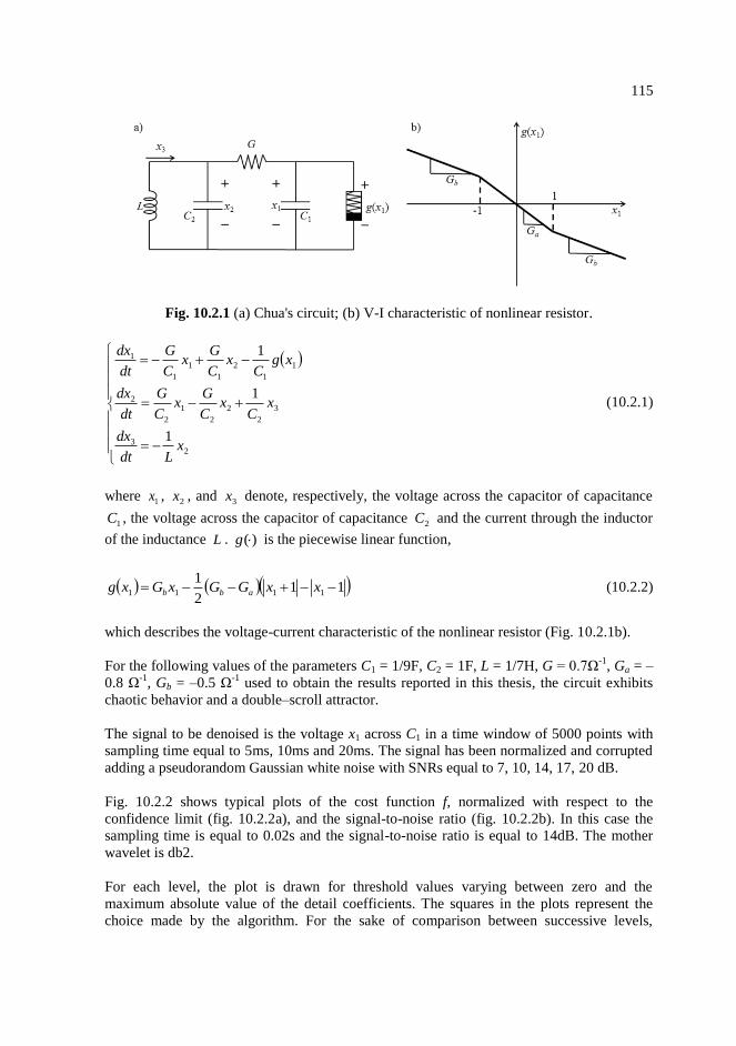
115
Fig. 10.2.1 (a) Chua's circuit; (b) V-I characteristic of nonlinear resistor.
23
3
2
2
2
1
2
2
1
1
2
1
1
1
1
1
1
1
xLdt
dx
xC
xC
Gx
C
G
dt
dx
xgC
xC
Gx
C
G
dt
dx
(10.2.1)
where 1x , 2x , and 3x denote, respectively, the voltage across the capacitor of capacitance
1C , the voltage across the capacitor of capacitance 2C and the current through the inductor
of the inductance L . )(g is the piecewise linear function,
112
11111 xxGGxGxg abb (10.2.2)
which describes the voltage-current characteristic of the nonlinear resistor (Fig. 10.2.1b).
For the following values of the parameters C1 = 1/9F, C2 = 1F, L = 1/7H, G = 0.7Ω-1
, Ga = –
0.8 Ω-1
, Gb = –0.5 Ω-1
used to obtain the results reported in this thesis, the circuit exhibits
chaotic behavior and a double–scroll attractor.
The signal to be denoised is the voltage x1 across C1 in a time window of 5000 points with
sampling time equal to 5ms, 10ms and 20ms. The signal has been normalized and corrupted
adding a pseudorandom Gaussian white noise with SNRs equal to 7, 10, 14, 17, 20 dB.
Fig. 10.2.2 shows typical plots of the cost function f, normalized with respect to the
confidence limit (fig. 10.2.2a), and the signal-to-noise ratio (fig. 10.2.2b). In this case the
sampling time is equal to 0.02s and the signal-to-noise ratio is equal to 14dB. The mother
wavelet is db2.
For each level, the plot is drawn for threshold values varying between zero and the
maximum absolute value of the detail coefficients. The squares in the plots represent the
choice made by the algorithm. For the sake of comparison between successive levels,
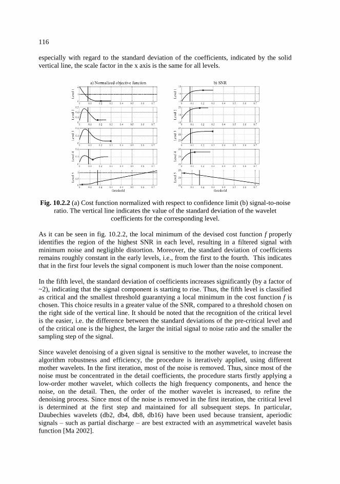
116
especially with regard to the standard deviation of the coefficients, indicated by the solid
vertical line, the scale factor in the x axis is the same for all levels.
Fig. 10.2.2 (a) Cost function normalized with respect to confidence limit (b) signal-to-noise
ratio. The vertical line indicates the value of the standard deviation of the wavelet
coefficients for the corresponding level.
As it can be seen in fig. 10.2.2, the local minimum of the devised cost function f properly
identifies the region of the highest SNR in each level, resulting in a filtered signal with
minimum noise and negligible distortion. Moreover, the standard deviation of coefficients
remains roughly constant in the early levels, i.e., from the first to the fourth. This indicates
that in the first four levels the signal component is much lower than the noise component.
In the fifth level, the standard deviation of coefficients increases significantly (by a factor of
~2), indicating that the signal component is starting to rise. Thus, the fifth level is classified
as critical and the smallest threshold guarantying a local minimum in the cost function f is
chosen. This choice results in a greater value of the SNR, compared to a threshold chosen on
the right side of the vertical line. It should be noted that the recognition of the critical level
is the easier, i.e. the difference between the standard deviations of the pre-critical level and
of the critical one is the highest, the larger the initial signal to noise ratio and the smaller the
sampling step of the signal.
Since wavelet denoising of a given signal is sensitive to the mother wavelet, to increase the
algorithm robustness and efficiency, the procedure is iteratively applied, using different
mother wavelets. In the first iteration, most of the noise is removed. Thus, since most of the
noise must be concentrated in the detail coefficients, the procedure starts firstly applying a
low-order mother wavelet, which collects the high frequency components, and hence the
noise, on the detail. Then, the order of the mother wavelet is increased, to refine the
denoising process. Since most of the noise is removed in the first iteration, the critical level
is determined at the first step and maintained for all subsequent steps. In particular,
Daubechies wavelets (db2, db4, db8, db16) have been used because transient, aperiodic
signals – such as partial discharge – are best extracted with an asymmetrical wavelet basis
function [Ma 2002].
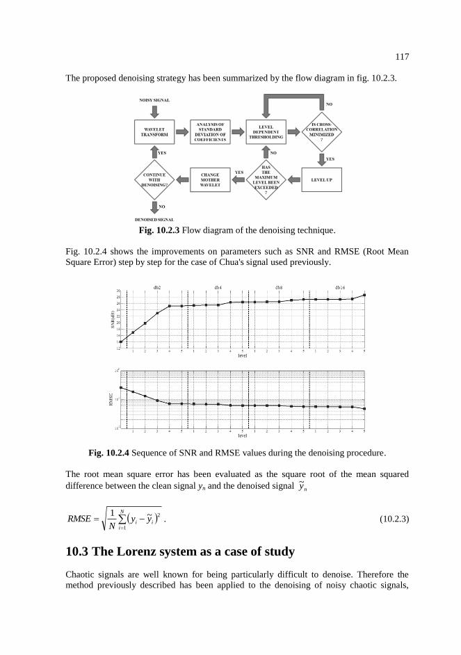
117
The proposed denoising strategy has been summarized by the flow diagram in fig. 10.2.3.
Fig. 10.2.3 Flow diagram of the denoising technique.
Fig. 10.2.4 shows the improvements on parameters such as SNR and RMSE (Root Mean
Square Error) step by step for the case of Chua's signal used previously.
Fig. 10.2.4 Sequence of SNR and RMSE values during the denoising procedure.
The root mean square error has been evaluated as the square root of the mean squared
difference between the clean signal yn and the denoised signal ny~
N
iii yy
NRMSE
1
2~1. (10.2.3)
10.3 The Lorenz system as a case of study
Chaotic signals are well known for being particularly difficult to denoise. Therefore the
method previously described has been applied to the denoising of noisy chaotic signals,

118
obtained by adding a white gaussian noise to the chaotic signals. As a typical example, in
the following the results obtained for Lorenz system [Lorenz 1963] have been reported. In
this case, as in practical cases, the added noise is considered unknown and is not used for the
denoising procedure.
The dynamics of the Lorenz system is described by
3213
2312
121
xxxdt
dx
xxxdt
dx
xxdt
dx
(10.3.1)
where σ is the Prandtl number, ρis the Rayleigh number and β is related to the horizontal
wavenumber of the convective motions. All σ, ρ, β > 0, but usually σ = 10, β = 8/3, and ρ is
varied. The system exhibits chaotic behavior for ρ = 28.
The signal to be denoised is the variable x1 in a time window of 5000 points with sampling
time equal to 5ms, 10ms and 20ms. The signal has been normalized and corrupted adding a
pseudorandom white gaussian noise with SNRs equal to 7, 10, 14, 17, 20 dB.
For each SNR, ten denoising sessions have been performed varying the added noise. Fig.
10.3.1 summarizes the simulation results in terms of mean value and minimum-maximum
values of SNR and RMSE.
Fig. 10.3.1 Simulation results for Lorenz system. The y–axis reports the SNR (a) and the
RMSE (b) of the denoised signal versus the SNR of the original signal with different
sampling times.
As expected, the denoising performance is strongly influenced by the signal sampling time.
In particular, the higher the ratio between the sampling frequency and the signal bandwidth,
the greater the increase in the signal-to-noise ratio.

119
Let us consider the case of a SNR before denoising of 14dB and sampling time equal to
0.01s. Fig. 10.3.2 shows the standard deviation of the detail coefficients at the different
decomposition levels during the first iteration of the algorithm. The standard deviation is
almost constant in the first three levels, whereas it considerably increases in the fourth level.
Thus, level four is the critical level.
Fig. 10.3.2 Standard deviation of details coefficients for each level in the first iteration with
mother wavelet db2.
Fig. 10.3.3 shows the values of SNR and RMSE in the different steps of the procedure. The
curve of SNR values is monotonic increasing and that one of RMSE values is monotonic
decreasing, confirming the suitability of the proposed approach.
Fig. 10.3.3 Sequence of SNR and RMSE values during the denoising procedure for the
Lorenz signal.
Table 10.3.1 reports the obtained results, in terms of SNR and RMSE, and those presented
in literature. As it can be noticed, the performance of the proposed method is slightly worse
with respect to that of the improved noise reduction method described in [Han 2009].
However, there is a crucial difference between the significance of the results in the two

120
cases. In [Han 2009] the optimal decomposition scale has been chosen in order to obtain the
minimal noise residual ratio, that can be evaluated only if the noiseless signal is known.
Since it is strongly problem-dependent, this method cannot be applied in real situations
when only the noisy signal is available.
Table 10.3.1 SNR and RMSE comparison of four denoising methods.
Method SNR after denoising (dB) RMSE
[Han 2006] 23.18 0.5431
[Han 2009] 24.60 0.4550
[Gao 2010] - 0.4803
Present method 24.20 0.4794
To provide a visual representation of the quality of the obtained results, in fig. 10.3.4 three
noisy signals are plotted. Fig. 10.3.4a shows the signal of the Lorenz system with a SNR
before denoising of 14dB with different sampling times (5ms, 10ms and 20ms); the related
denoised signals are reported in Fig. 10.3.4b.
Fig. 10.3.4 Lorenz: x1 time series (a) noisy data (SNR=14 dB), (b) denoised data.
10.4 Application to time series from JET diagnostics
The algorithm has been applied to real signals coming from the soft X-rays diagnostic of the
tokamak JET during an ELM. It is important to consider that, in presence of real noisy
signals, the form and the values of the noise are not known, and make quantitative
considerations on the signal to noise ratio or mean square error is not possible. It is therefore
necessary, in these cases, in order to make qualitative considerations on the success of the
denoising method, to be able to distinguish, roughly at least, the noise component from the
signal one.
The denoising technique has been applied to a time series of 20000 samples with sampling
time Ts = 100μs. In fig. 10.4.1, the time series before and after denoising and the the
residuals are shown.
0 5 10 15 20 25
-20
-10
0
10
20
a) Noisy signal
Ts = 5ms
0 5 10 15 20 25
-20
-10
0
10
20
b) Denoised signal
0 5 10 15 20 25
-20
-10
0
10
20
Ts = 10ms
0 5 10 15 20 25
-20
-10
0
10
20
0 5 10 15 20 25
-20
-10
0
10
20
Ts = 20ms
time (s)0 5 10 15 20 25
-20
-10
0
10
20
time (s)
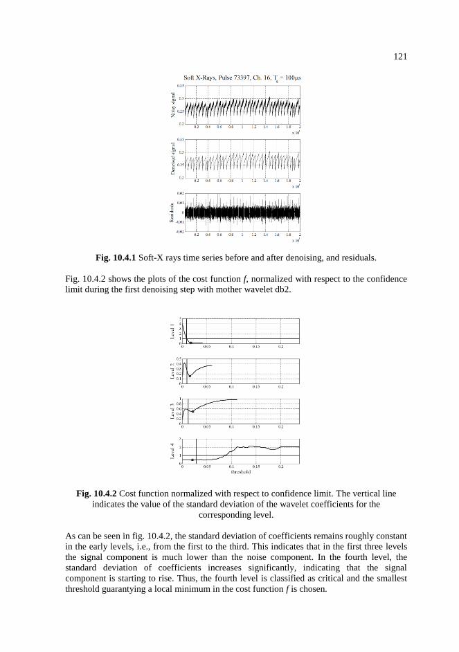
121
Fig. 10.4.1 Soft-X rays time series before and after denoising, and residuals.
Fig. 10.4.2 shows the plots of the cost function f, normalized with respect to the confidence
limit during the first denoising step with mother wavelet db2.
Fig. 10.4.2 Cost function normalized with respect to confidence limit. The vertical line
indicates the value of the standard deviation of the wavelet coefficients for the
corresponding level.
As can be seen in fig. 10.4.2, the standard deviation of coefficients remains roughly constant
in the early levels, i.e., from the first to the third. This indicates that in the first three levels
the signal component is much lower than the noise component. In the fourth level, the
standard deviation of coefficients increases significantly, indicating that the signal
component is starting to rise. Thus, the fourth level is classified as critical and the smallest
threshold guarantying a local minimum in the cost function f is chosen.

122
10.5 Conclusions
A new denoising method based on the wavelet transform of the noisy signal and on the
cross-correlation between the denoised signal and the residuals has been developed. This
procedure, in contrast to previous works, is suitable to denoising signals in real situations,
when the noiseless signal is not known.
Several tests on chaotic signals have been performed varying the sampling step and the
initial amount of noise. The technique has proved to be quite robust and has allowed
increasing the signal-to-noise ratio of a quantity dependent only on the ratio between the
sampling frequency and the bandwidth of the signal. The performance obtained is quite
competitive with respect to the most recent alternative methods that, on the other hand, are
not applicable to experimental signals.
With regard to practical applications, the developed algorithms has been applied also to
experimental time series coming from JET database. The application to experimental time
series has led the method to deal with the normal difficulties encountered in these cases, like
the presence of non-white noise and a not clear discrimination between the signal and the
noise component. In these cases, the algorithm has been able to eliminate only the white
component of the noise, while keeping the non-white one unaltered.

123
Chapter 11
Dynamic behaviour of Type I ELMs
This chapter deals with the study of dynamic behaviour of Type I ELMs. The final goal of
the study is the modelization of the phenomenon.
As a first step, a statistical analysis of time intervals between successive Type I ELMs is
proposed. The analysis can be summarized in the following steps: database construction
(section 11.1), ELMs detection (section 11.2), i.e., identification of inter-ELM time
intervals, distribution fitting on the entire sample of time intervals (section 11.3),
memorylessness study on the best fit distribution (section 11.4), analysis of variance
(section 11.5), grouping of pulses obtained in similar experimental conditions and detailed
analysis on some groups (section 11.6), determinism analysis on ELM time series (section
11.7).
11.1 Database construction
For the analysis, a database of 60 shots has been analysed. The D signals taken from the
outer divertor line of sight have been used, resulting in a total of 3448 Type I ELMs
extracted from JET database, sampled with a time step of 100s.
Only the shots in which the plasma conditions are stable and stationary have been selected.
For the analysis of stationarity, plasma current, vacuum toroidal field at R=2.96, neutral
beam input power and lower triangularity have been considered as the input quantities of
interest.
For the sake of stationarity, only cases in which the heating power of the plasma was given
by only two contributions, ohmic power and neutral beam power, have been used, since the
greatest contribution to the variation of the input power is given by radiofrequency and LH-
waves heating.
The neutral beam power contribution is the main cause of ELMs generation, since it allows
the L-H transition. In addition, all experiments dealing with ELM control and mitigation
techniques have been avoided.
Pulses used for the analysis have been selected within the campaigns between C21 and
C27b (from 9th
June 2008 to 23rd
October 2010). In table 11.1.1, a list of the experiments
candidates for the analysis has been reported.
The level of accuracy of the different input signals has been considered for the verification
of stationarity of the input space. Fig. 11.1.1 shows the orthogonal projections of the input
space for each pulse.
As shown in fig. 11.1.1, there is a slight correlation between the plasma current and the
toroidal magnetic field. This doesn’t result from a physical relationship, but from
experimental conditions.
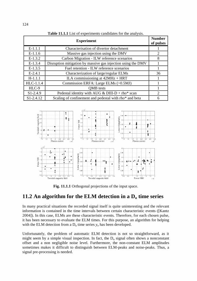
124
Table 11.1.1 List of experiments candidates for the analysis.
Experiment Number
of pulses
E-1.1.1 Characterisation of divertor detachment 1
E-1.1.6 Massive gas injection using the DMV 2
E-1.3.2 Carbon Migration - ILW reference scenarios 8
E-1.3.4 Disruption mitigation by massive gas injection using the DMV 1
E-1.3.5 Fuel retention - ILW reference scenarios 1
E-2.4.1 Characterization of large/regular ELMs 36
H-1.1.1 ILA commissioning at 42MHz + HRT 1
HLC-1.1.4 Commission ERFA: Large ELMs (>0.5MJ) 1
HLC-9 QMB tests 1
S1-2.4.9 Pedestal identity with AUG & DIII-D + rho* scan 2
S1-2.4.12 Scaling of confinement and pedestal with rho* and beta 6
Fig. 11.1.1 Orthogonal projections of the input space.
11.2 An algorithm for the ELM detection in a Dα time series
In many practical situations the recorded signal itself is quite uninteresting and the relevant
information is contained in the time intervals between certain characteristic events ([Kantz
2004]). In this case, ELMs are these characteristic events. Therefore, for each chosen pulse,
it has been necessary to evaluate the ELM times. For this purpose, an algorithm for helping
with the ELM detection from a Dα time series yn has been developed.
Unfortunately, the problem of automatic ELM detection is not so straightforward, as it
might seem by a simple visual inspection. In fact, the Dα signal often shows a nonconstant
offset and a non negligible noise level. Furthermore, the non-constant ELM amplitudes
sometimes makes it difficult to distinguish between ELM-peaks and noise-peaks. Thus, a
signal pre-processing is needed.
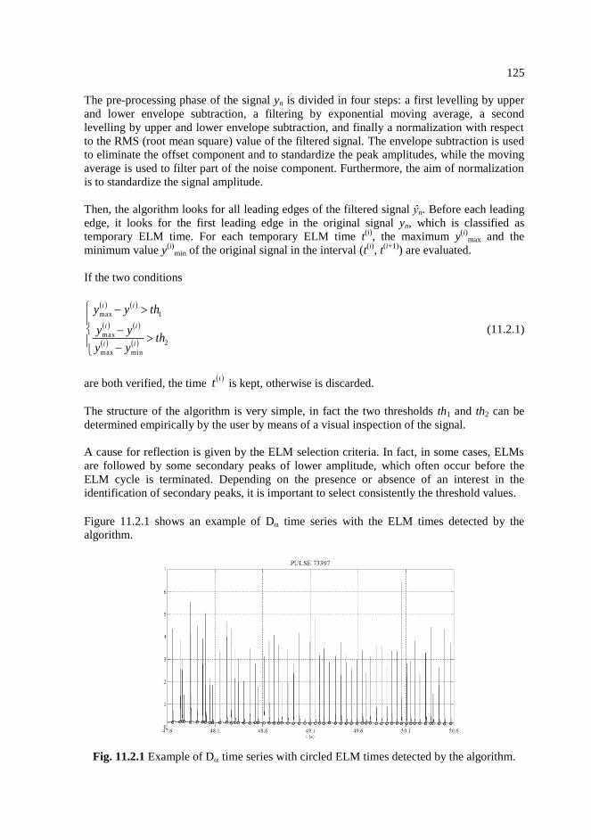
125
The pre-processing phase of the signal yn is divided in four steps: a first levelling by upper
and lower envelope subtraction, a filtering by exponential moving average, a second
levelling by upper and lower envelope subtraction, and finally a normalization with respect
to the RMS (root mean square) value of the filtered signal. The envelope subtraction is used
to eliminate the offset component and to standardize the peak amplitudes, while the moving
average is used to filter part of the noise component. Furthermore, the aim of normalization
is to standardize the signal amplitude.
Then, the algorithm looks for all leading edges of the filtered signal ŷn. Before each leading
edge, it looks for the first leading edge in the original signal yn, which is classified as
temporary ELM time. For each temporary ELM time t(i)
, the maximum y(i)
max and the
minimum value y(i)
min of the original signal in the interval (t(i)
, t(i+1)
) are evaluated.
If the two conditions
2
minmax
max
1max
thyy
yy
thyy
ii
ii
ii
(11.2.1)
are both verified, the time it is kept, otherwise is discarded.
The structure of the algorithm is very simple, in fact the two thresholds th1 and th2 can be
determined empirically by the user by means of a visual inspection of the signal.
A cause for reflection is given by the ELM selection criteria. In fact, in some cases, ELMs
are followed by some secondary peaks of lower amplitude, which often occur before the
ELM cycle is terminated. Depending on the presence or absence of an interest in the
identification of secondary peaks, it is important to select consistently the threshold values.
Figure 11.2.1 shows an example of D time series with the ELM times detected by the
algorithm.
Fig. 11.2.1 Example of D time series with circled ELM times detected by the algorithm.
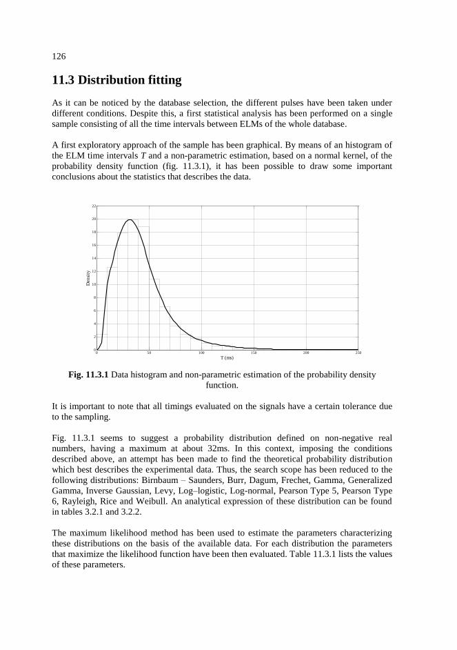
126
11.3 Distribution fitting
As it can be noticed by the database selection, the different pulses have been taken under
different conditions. Despite this, a first statistical analysis has been performed on a single
sample consisting of all the time intervals between ELMs of the whole database.
A first exploratory approach of the sample has been graphical. By means of an histogram of
the ELM time intervals T and a non-parametric estimation, based on a normal kernel, of the
probability density function (fig. 11.3.1), it has been possible to draw some important
conclusions about the statistics that describes the data.
Fig. 11.3.1 Data histogram and non-parametric estimation of the probability density
function.
It is important to note that all timings evaluated on the signals have a certain tolerance due
to the sampling.
Fig. 11.3.1 seems to suggest a probability distribution defined on non-negative real
numbers, having a maximum at about 32ms. In this context, imposing the conditions
described above, an attempt has been made to find the theoretical probability distribution
which best describes the experimental data. Thus, the search scope has been reduced to the
following distributions: Birnbaum – Saunders, Burr, Dagum, Frechet, Gamma, Generalized
Gamma, Inverse Gaussian, Levy, Log–logistic, Log-normal, Pearson Type 5, Pearson Type
6, Rayleigh, Rice and Weibull. An analytical expression of these distribution can be found
in tables 3.2.1 and 3.2.2.
The maximum likelihood method has been used to estimate the parameters characterizing
these distributions on the basis of the available data. For each distribution the parameters
that maximize the likelihood function have been then evaluated. Table 11.3.1 lists the values
of these parameters.
0 50 100 150 200 2500
2
4
6
8
10
12
14
16
18
20
22
T (ms)
Den
sity

127
Table 11.3.1 List of distributions and best fit parameters.
Distribution Parameters Distribution Parameters
Birnbaum–Saunders α = 0.60436
β = 0.03572 Log–Logistic
α = 3.1142
β = 0.03613
Burr
k = 1.8386
α = 2.6275
β = 0.0507
Log–Normal σ = 0.57689
μ = −3.3201
Dagum
k = 0.62246
α = 3.7915
β = 0.0457
Pearson Type 5 α = 2.9575
β = 0.08943
Frechet α = 2.102
β = 0.02747 Pearson Type 6
α1 = 4.2771
α2 = 15.042
β = 0.13881
Gamma α = 2.9672
β = 0.01425 Rayleigh σ = 0.03375
Generalized Gamma
k = 1.0329
α = 3.0991
β = 0.01425
Rice ν = 1.5110 · 10
−5
σ = 0.03458
Inverse Gaussian λ = 0.12549
μ = 0.04229 Weibull
α = 2.1846
β = 0.04703
Levy σ = 0.03024
Table 11.3.2 Results of tests for each theoretical model. Highlighted in grey distributions
for which the K-S test has given a positive result.
Distribution K
Kcr5%
= 0.0231 AIC BIC Distribution
K Kcr
5% = 0.0231
AIC BIC
Birnbaum–
Saunders 0.0579 -16855 -16842
Log-
Logistic 0.0509 -16901 -16888
Burr 0.0183 -16976 -16957 Log-
Normal 0.0443 -16900 -16888
Dagum 0.0165 -16964 -16946 Pearson
Type 5 0.0881 -16460 -16447
Frechet 0.1135 -14985 -14972 Pearson
Type 6 0.0246 -16968 -16949
Gamma 0.0362 -16899 -16887 Rayleigh 0.0621 -16602 -16595
Generalized
Gamma 0.0386 -16917 -16899 Rice 0.0799 -16608 -16596
Inverse
Gaussian 0.0418 -16768 -16756 Weibull 0.0507 -16363 -16351
Levy 0.3935 -12493 -12487
The verification of conformity of the observed data to the different theoretical models, i.e.,
the goodness of fit, has been carried out using three statistical test. In this particular case, the
Kolmogorov–Smirnov (K–S) test, the Akaike Information Criterion (AIC) and the Bayesian
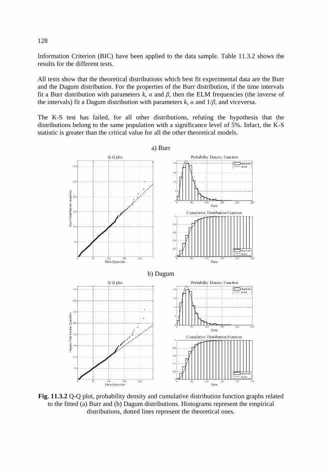
128
Information Criterion (BIC) have been applied to the data sample. Table 11.3.2 shows the
results for the different tests.
All tests show that the theoretical distributions which best fit experimental data are the Burr
and the Dagum distribution. For the properties of the Burr distribution, if the time intervals
fit a Burr distribution with parameters k, α and β, then the ELM frequencies (the inverse of
the intervals) fit a Dagum distribution with parameters k, α and 1/β, and viceversa.
The K-S test has failed, for all other distributions, refuting the hypothesis that the
distributions belong to the same population with a significance level of 5%. Infact, the K-S
statistic is greater than the critical value for all the other theoretical models.
a) Burr
b) Dagum
Fig. 11.3.2 Q-Q plot, probability density and cumulative distribution function graphs related
to the fitted (a) Burr and (b) Dagum distributions. Histograms represent the empirical
distributions, dotted lines represent the theoretical ones.

129
Fig. 11.3.2 shows the Q-Q plots and the probability density and cumulative distribution
function graphs related to the fitted Burr and Dagum distributions.
The Q-Q plots confirm visibly the obtained results. Moreover they show that the Burr
distribution fits the sample better than the Dagum distribution, even if the previous test
values are very similar. Thus, given these considerations, it can be said that the sample
intervals are most likely to belong to a Burr distribution, and that the ELM frequencies fit a
Dagum distribution with parameters k = 1.8386, α = 2.6275 and β = 19.724.
11.4 Memorylessness study
As it can be noticed, the statistics is very far from the one described by an exponential
distribution, which is well known for its memorylessness property, allowing the hypothesis
of presence of memory between subsequent ELMs.
The conditional probability that the value of T is smaller than T1 + T2, given that it is larger
than or equal to T1 is
1
121
1
211121
1Pr
PrPr
TF
TFTTF
TT
TTTTTTTTT
(11.4.1)
has been evaluated on the entire sample, and its dependency on the variable T1 has been
used as an indicator of the presence of memory. Fig. 11.4.1 shows the conditional
probability for the model Burr distribution with respect to the variables T1 and T2.
Fig. 11.4.1 Contour plot of probability Pr{T T1+T2/ T T1} with respect to T1 and T2.
If α is the conditional probability (11.4.1), the contour line in fig. 11.4.1 related to α
represents the values of T1 and T2 for which the conditional probability Pr{T T1 + T2/ T
T1} = α. For example, the last contour line on the top is related to α = 99%. Thus, looking at
the point (0.15, 0.25) in the graph, if after T1 = 0.15s no ELM has occurred, then there is a
99% probability that the next ELM occurs within other T2 = 0.25s. As it can be noticed from
the contour lines, the dependence on the variable T1 is not negligible, thus the process is not
T1 (s)
T2 (
s)
Memory
0 0.05 0.1 0.15 0.2 0.250
0.05
0.1
0.15
0.2
0.25
0.8
0.7
0.6
0.5
0.4
0.30.20.1
0.9
0.95
0.99

130
memoryless. In fact, if the process was memoryless, the contour lines would be parallel to
the x-axis, indicating no dependence on T1.
11.5 Analysis of variance
All the considerations made previously have been made assuming that the intervals in each
pulse belong to the same population. But the question is to check whether this assumption is
correct or not, and if the different experimental conditions affect their statistical behaviour.
The technique typically used to decide whether the different samples belong to the same
population is the analysis of variance (ANOVA). In the present case, the hypothesis that all
samples belong to a population having a normal distribution cannot be met, because time
intervals are positive quantities which cannot be described by a distribution defined also for
negative values. For these reasons, it has been necessary to use the Kruskal-Wallis test.
The Kruskal-Wallis test has been applied to the observations of ELM intervals from all
pulses. For the test samples, the H statistic has been given as H = 1981.4. This value has
been compared with the critical value Hcr5%
= 77.93, obtained by evaluating the inverse
cumulative distribution function of a chi-squared distribution with 59 degrees of freedom for
the probability 0.95. Because %5
crHH , the null hypothesis, whereby the samples come
from the same population, has been rejected at the significance level 5%.
11.6 Grouping pulses
11.6.1 Grouping by input signals
Given the previous results, pulses relative to similar inputs have been grouped, taking into
account the signals’ tolerances (4% for toroidal magnetic field, 2% for plasma current, 10%
for NBI input power and lower triangularity). In particular, two input conditions have been
considered similar if all the input parameters have fallen within the limits dictated by their
tolerance, that is
k
k
jk
ik
tol
tol
u
u
1
1loglog , (11.6.1)
where uik and ujk are respectively the input k of pulses i and j and tolk is the relative tolerance
related to the input k. A set of pulses belong to a group if each pair of pulses belonging to
the group is characterized by similar input conditions. It has been possible to distinguish
between three different cases: single pulses, pairs of pulses and cliques (groups of three or
more pulses).
The algorithm used for finding cliques is reported in [Harary 1957].
From the initial 60 pulses, 21 groups have been created, including 4 singles, 3 pairs and 14
cliques. Table 11.6.1 reports the obtained groups. For each group, the number of samples,
the input conditions and the result of the Kruskal-Wallis test with 5% confidence level are
reported.

131
Table 11.6.1 Groups with division by input conditions.
G Pulses ni Inputs
K-W
test
(5%)
1 73397, 73445, 73446, 73447,
73450, 73484, 74130 432
2.5MA, 2.4T,
12.5-14.8MW, 0.23-0.28 NO
2 73397, 73484, 74376 200 2.5MA, 2.4-2.5T,
14.5-15.1MW, 0.27-0.33 NO
3 74364, 76812 176 2MA, 1.8T,
15.5-18.5MW, 0.36-0.37 NO
4 74365, 74366, 74367, 74368,
74369, 74371, 74372, 74373,
74374, 74375, 74443
395 2.5MA, 2.5-2.7T,
15.5-18.5MW, 0.32-0.35 NO
5 74365, 74366, 74367, 74368,
74369, 74371, 74372, 74373,
74374, 74375, 77073
468 2.5-2.6MA, 2.4-2.5T,
15.5-18.5MW, 0.34-0.36 NO
6 74375, 74376, 74443, 74444 144 2.5MA, 2.5-2.7T,
14-15.8MW, 0.32-0.35 NO
7 74375, 74376, 78448 73 2.5MA, 2.5-2.7T,
12.9-15.5MW, 0.33-0.4 NO
8 '74375, 74376, 77073 175 2.5-2.6MA, 2.4-2.5T,
15.1-17MW, 0.33-0.36 NO
9 74378, 75724, 75726, 75727,
75728, 75731, 75732, 76481,
79389
629 2MA, 2T,
11-12.8MW, 0.32-0.37 NO
10 74378, 75724, 75726, 75727,
75728, 75731, 75732, 76476,
79389
629 2MA, 2T,
11.9-14.5MW, 0.32-0.37 NO
11 74378, 75724, 75728, 75731,
75732, 76473, 76474, 76475,
76476, 76477, 76478, 76479
705 2MA, 2T,
12.5-15.2MW, 0.32-0.37 NO
12 74612, 74613, 77073 291 2.6MA, 2.3-2.4T, 16.7-17MW, 0.36 NO
13 74793, 74795 286 1.7MA, 1.6T,
9.1-10.5MW, 0.35-0.36 NO
14 74798 120 1.7MA, 1.6T, 16.8MW, 0.37 /
15 75118 33 1.7MA, 1.8T, 9.4MW, 0.26 NO
16 75724, 75728, 76471, 76472,
76473, 76474, 76475, 76476,
76477, 76478, 76479
439 2MA, 2T,
12.6-15.4MW, 0.32-0.37 NO
17 76428, 76430, 76431, 76437,
76438, 76440, 76443, 77192 323
2MA, 2T,
7.5-8.4MW, 0.31-0.36 NO
18 76470, 76480 45 2MA, 2T,
16.8-19.8MW, 0.37 NO
19 76470, 76471, 76472, 76473,
76474, 76475, 76476, 76477,
76478, 76479
363 2MA, 2T,
14.5-16.8MW, 0.35-0.37 YES
20 78750 104 1.5MA, 1.8T, 17.6MW, 0.32 NO
21 79546 177 1.5MA, 1.8T, 17.7MW, 0.45 NO

132
As it can be noticed, there are several multicliqual pulses. Moreover, only for one group
(19) the Kruskal-Wallis test has given a positive result.
11.6.2 Grouping by input signals and experiments
A more selective division between the groups has been made by discriminating pulses with
similar input conditions but coming from different experiments. By means of this division,
from the initial 60 pulses, 24 groups have been created, including 10 singles, 4 pairs and 10
cliques. In table 11.6.2, the groups are listed. For each group, the number of samples, the
input conditions, the name of the experiment and the result of the Kruskal-Wallis test with
5% confidence level are reported.
Table 11.6.2 Groups with division by input conditions and experiment.
G Pulses ni Inputs Exp.
K-W
test
(5%)
1 73397, 73445, 73446,
73447, 73450 246
2.5MA, 2.4T,
12.5-14.5MW, 0.23-0.27 E-1.3.2 NO
2 73484 108 2.5MA, 2.4T, 14.8MW, 0.28 E-1.3.2 NO
3 74130 78 2.5MA, 2.4T, 13.6MW, 0.25 E-1.3.2 NO
4 74364 116 2MA, 1.8T, 15.5MW, 0.36 E-1.3.2 NO
5
74365, 74366, 74367,
74368, 74369, 74371,
74372, 74373, 74374,
74375
347 2.5MA, 2.5T,
15.5-18.5MW, 0.34-0.35 E-1.3.2 NO
6 74375, 74376 54 2.5MA, 2.5T,
15.1-15.5MW, 0.33-0.35 E-1.3.5 YES
7 74378, 75724, 75726,
75727, 75728, 75731,
75732, 76481
497 2MA, 2T,
11-12.8MW, 0.32-0.37 HLC-9 NO
8 74378, 75724, 75726,
75727, 75728, 75731,
75732, 76476
497 2MA, 2T,
12.1-14.5MW, 0.32-0.37 E-2.4.1 NO
9
74378, 75724, 75728,
75731, 75732, 76473,
76474, 76475, 76476,
76477, 76478, 76479
705 2MA, 2T,
12.5-15.2MW, 0.32-0.37 E-2.4.1 NO
10 74443, 74444 90 2.5MA, 2.7T, 14-15.8MW, 0.32 E-2.4.1 YES
11 74612, 74613, 77073 291 2.6MA, 2.3-2.4T,
16.7-17MW, 0.36 E-2.4.1 NO
12 74793, 74795 286 1.7MA, 1.6T,
9.1-10.5MW, 0.35-0.36 E-2.4.1 NO
13 74798 120 1.7MA, 1.6T, 16.8MW, 0.37 E-2.4.1 NO
14 75118 33 1.7MA, 1.8T, 9.4MW, 0.26 E-2.4.1 NO
15
75724, 75728, 76471,
76472, 76473, 76474,
76475, 76476, 76477,
76478, 76479
439 2MA, 2T,
12.6-15.4MW, 0.32-0.37 E-2.4.1 NO
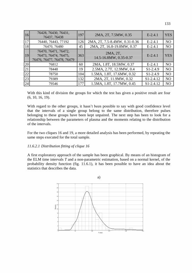
133
16 76428, 76430, 76431,
76437, 76438 197 2MA, 2T, 7.5MW, 0.35 E-2.4.1 YES
17 76440, 76443, 77192 126 2MA, 2T, 7.5-8.4MW, 0.31-0.36 E-2.4.1 NO
18 76470, 76480 45 2MA, 2T, 16.8-19.8MW, 0.37 E-2.4.1 NO
19 76470, 76471, 76472,
76473, 76474, 76475,
76476, 76477, 76478, 76479
363 2MA, 2T,
14.5-16.8MW, 0.35-0.37 E-2.4.1 YES
20 76812 60 2MA, 1.8T, 18.5MW, 0.37 E-2.4.1 NO
21 78448 19 2.5MA, 2.7T, 12.9MW, 0.4 S1-2.4.9 NO
22 78750 104 1.5MA, 1.8T, 17.6MW, 0.32 S1-2.4.9 NO
23 79389 132 2MA, 2T, 11.9MW, 0.32 S1-2.4.12 NO
24 79546 177 1.5MA, 1.8T, 17.7MW, 0.45 S1-2.4.12 NO
With this kind of division the groups for which the test has given a positive result are four
(6, 10, 16, 19).
With regard to the other groups, it hasn’t been possible to say with good confidence level
that the intervals of a single group belong to the same distribution, therefore pulses
belonging to these groups have been kept unpaired. The next step has been to look for a
relationship between the parameters of plasma and the moments relating to the distribution
of the intervals.
For the two cliques 16 and 19, a more detailed analysis has been performed, by repeating the
same steps executed for the total sample.
11.6.2.1 Distribution fitting of clique 16
A first exploratory approach of the sample has been graphical. By means of an histogram of
the ELM time intervals T and a non-parametric estimation, based on a normal kernel, of the
probability density function (fig. 11.6.1), it has been possible to have an idea about the
statistics that describes the data.
a)
0 50 100 150 200 2500
2
4
6
8
10
12
14
16
18
20
22
T (ms)
Densi
ty
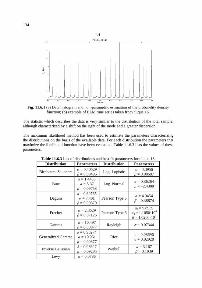
134
b)
Fig. 11.6.1 (a) Data histogram and non-parametric estimation of the probability density
function; (b) example of ELM time series taken from clique 16.
The statistic which describes the data is very similar to the distribution of the total sample,
although characterized by a shift on the right of the mode and a greater dispersion.
The maximum likelihood method has been used to estimate the parameters characterizing
the distributions on the basis of the available data. For each distribution the parameters that
maximize the likelihood function have been evaluated. Table 11.6.3 lists the values of these
parameters.
Table 11.6.3 List of distributions and best fit parameters for clique 16.
Distribution Parameters Distribution Parameters
Birnbaum–Saunders α = 0.40529
β = 0.08496 Log–Logistic
α = 4.3956
β = 0.08687
Burr
k = 1.4485
α = 5.37
β = 0.09753
Log–Normal σ = 0.36264
μ = –2.4388
Dagum
k = 0.60765
α = 7.401
β = 0.09879
Pearson Type 5 α = 4.9454
β = 0.38874
Frechet α = 2.8629
β = 0.07126 Pearson Type 6
α1 = 9.8939
α2 = 1.1050·108
β = 1.0260·106
Gamma α = 10.497
β = 0.00877 Rayleigh σ = 0.07344
Generalized Gamma
k = 0.98274
α = 10.061
β = 0.00877
Rice υ = 0.08696
σ = 0.02928
Inverse Gaussian λ = 0.96627
μ = 0.09205 Weibull
α = 3.167
β = 0.1039
Levy σ = 0.0786
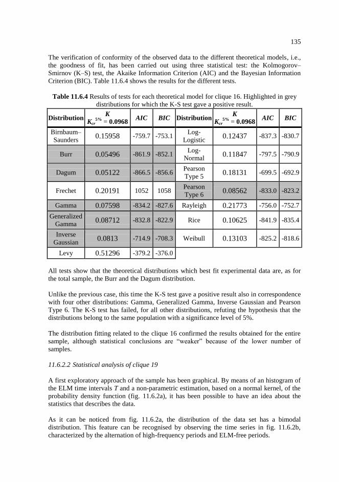
135
The verification of conformity of the observed data to the different theoretical models, i.e.,
the goodness of fit, has been carried out using three statistical test: the Kolmogorov–
Smirnov (K–S) test, the Akaike Information Criterion (AIC) and the Bayesian Information
Criterion (BIC). Table 11.6.4 shows the results for the different tests.
Table 11.6.4 Results of tests for each theoretical model for clique 16. Highlighted in grey
distributions for which the K-S test gave a positive result.
Distribution K
Kcr5%
= 0.0968 AIC BIC Distribution
K Kcr
5% = 0.0968
AIC BIC
Birnbaum–
Saunders 0.15958 -759.7 -753.1
Log-
Logistic 0.12437 -837.3 -830.7
Burr 0.05496 -861.9 -852.1 Log-
Normal 0.11847 -797.5 -790.9
Dagum 0.05122 -866.5 -856.6 Pearson
Type 5 0.18131 -699.5 -692.9
Frechet 0.20191 1052 1058 Pearson
Type 6 0.08562 -833.0 -823.2
Gamma 0.07598 -834.2 -827.6 Rayleigh 0.21773 -756.0 -752.7
Generalized
Gamma 0.08712 -832.8 -822.9 Rice 0.10625 -841.9 -835.4
Inverse
Gaussian 0.0813 -714.9 -708.3 Weibull 0.13103 -825.2 -818.6
Levy 0.51296 -379.2 -376.0
All tests show that the theoretical distributions which best fit experimental data are, as for
the total sample, the Burr and the Dagum distribution.
Unlike the previous case, this time the K-S test gave a positive result also in correspondence
with four other distributions: Gamma, Generalized Gamma, Inverse Gaussian and Pearson
Type 6. The K-S test has failed, for all other distributions, refuting the hypothesis that the
distributions belong to the same population with a significance level of 5%.
The distribution fitting related to the clique 16 confirmed the results obtained for the entire
sample, although statistical conclusions are “weaker” because of the lower number of
samples.
11.6.2.2 Statistical analysis of clique 19
A first exploratory approach of the sample has been graphical. By means of an histogram of
the ELM time intervals T and a non-parametric estimation, based on a normal kernel, of the
probability density function (fig. 11.6.2a), it has been possible to have an idea about the
statistics that describes the data.
As it can be noticed from fig. 11.6.2a, the distribution of the data set has a bimodal
distribution. This feature can be recognised by observing the time series in fig. 11.6.2b,
characterized by the alternation of high-frequency periods and ELM-free periods.

136
a)
b)
Fig. 11.6.2 (a) Data histogram and non-parametric estimation of the probability density
function; (b) example of ELM time series taken from clique 19.
This special case hasn’t allow to confirm the characteristics of the distribution of the total
sample, strengthening the Kruskal – Wallis test results previously obtained in section 11.5.
11.7 Analysis of determinism of ELM time series
The previous analysis has shown that the statistical properties of the time intervals are
mostly dependent on the single time series. Then, an analysis of ELM time series may be
useful in order to highlight the presence of determinism.
For each Dα time series taken from the database, the Hurst exponent has been evaluated with
the purpose of detecting the presence of determinism within the ELM phenomenon. A
preliminary denoising of time series has been performed to eliminate the noise component
by the signal applying the algorithm proposed in chapter 10. In fig. 11.7.1 a histogram of
values obtained for the 60 denoised time series is shown.
10 20 30 40 50 60 700
5
10
15
20
25
30
35
40
45
50
55
T (ms)
Densi
ty

137
Fig. 11.7.1 Histogram of the Hurst exponent values for the different pulses.
As can be noticed, the Hurst exponent values are all located in the range between 0.5 and 1,
indicating a persistent behaviour. This result is very important for a future modelling of the
ELM phenomenon.
For 35 of the denoised Dα time series taken from the database, the maximum Lyapunov
exponent has been evaluated with the Rosenstein algorithm [Rosenstein 1993] developed for
Matlab in [Mohammadi 2009].
For the estimation of the maximum Lyapunov exponent, it has been necessary to reconstruct
the embedding space from each time series. This task is performed automatically by the
software. For the selection of the time delay methods of autocorrelation function and
minimum mutual information are used. Two methods, namely False Nearest Neighbors and
Symplectic Geometry, are used for choosing proper value of the embedding dimension. In
table 11.7.1 the list of pulses with the embedding parameters is shown.
Table 11.7.1 Estimated embedding parameters and maximum Lyapunov exponent for each
time series.
Pulse Time
Delay
Embedding
dimension
Maximum
Lyapunov
exponent
73397 8 5 0.0975
73445 9 10 0.0820
73446 8 5 0.0952
73447 8 5 0.0929
73450 1 4 0.1248
74365 1 8 0.1081
74366 1 5 0.1034
74368 1 6 0.0804
74369 1 5 0.0725
74371 1 7 0.1047
0.5 0.55 0.6 0.65 0.7 0.75 0.8 0.85 0.9 0.95 10
1
2
3
4
5
6
7
Hurst exponent

138
74373 1 5 0.0809
74374 1 8 0.1046
74376 1 6 0.0816
74443 1 6 0.1004
74613 1 5 0.0952
75118 7 4 0.0951
75724 1 4 0.0801
75726 1 9 0.1017
75727 1 16 0.1012
75732 1 5 0.1141
76438 1 4 0.0860
76470 9 3 0.0736
76471 8 12 0.0757
76473 1 8 0.1078
76474 1 11 0.0997
76475 1 10 0.1190
76477 1 3 0.1106
76478 1 2 0.0754
76479 1 4 0.0961
76480 1 4 0.1065
76481 1 3 0.1129
77073 1 2 0.1491
78448 1 9 0.0807
78750 7 7 0.0829
73397 8 5 0.0975
In fig. 11.7.2 a histogram of the obtained values is shown.
Fig. 11.7.2 Histogram of the maximum Lyapunov exponent values for the different pulses.
As can be noticed, the maximum Lyapunov exponent values are all positive, indicating the
possibility of a chaotic behaviour.
139
11.8 Conclusions
A statistical analysis of time intervals between successive Type I ELMs has been proposed.
For this purpose, a database of 60 shots, by using the D signals taken from the outer
divertor line of sight, has been created. Much attention has been given to the search of time
intervals in which the plasma conditions are stable and stationary. Firstly, an algorithm for
finding the ELM spikes in D-alpha time series has been developed. Then, the empirical
probability distribution of the entire sample of inter-ELM time periods has been fitted with
several theoretical distributions. Some statistical tests have been used for finding the best fit.
The tests have shown that Burr distribution is the one that best fits the experimental data.
A memorylessness analysis on the probability distribution recognized that the process is not
memoryless.
Finally, an analysis of variance on the entire database led to the conclusion that inter-ELM
time periods coming from different pulses don’t belong to the same population, i.e., the
statistical properties of the intervals are dependent on the single pulse.
A division of pulses depending on the type of experiment and on some parameters of plasma
has been performed. A statistical analysis on the two bigger groups confirmed the obtained
results.
A final analysis of ELM time series has been performed in order to highlight the presence of
determinism. In fact, the Hurst exponent evaluated for all the pulses, indicated the presence
of a persistent behaviour. This result is very important for a future modelling of the ELM
phenomenon. Furthermore, the evaluation of the maximum Lyapunov exponent has allowed
to hypothesize about the presence of a chaotic behaviour.

140
Conclusions
In this dissertation the solution of several engineering problems dealing with the analysis
and synthesis of complex systems has been addressed.
In particular, a new algorithm which optimizes Lyapunov exponents estimation in piecewise
linear systems has been applied on PWL and polynomial chaotic systems. In the case of
polynominal systems, firstly, a suitable piecewise linear approximation for the polynomial
nonlinear function has been evaluated by means of a Multi-Layer Perceptron (MLP) neural
network with linear and saturating linear transfer functions. Then, the piecewise linearity of
the state equation has been exploited to evaluate Lyapunov exponents of the approximated
system. Results show that the algorithm is able to accurately estimate the exponents strongly
reducing the execution time.
In the field of complex systems synthesis, a systematic method to project systems of order
2n characterized by two positive Lyapunov exponents, has been proposed. This procedure
couples nth-order chaotic systems with a suitable non linear coupling function. Examples of
polynomial and piecewise linear systems have been proposed. Both numerical simulation
and circuit implementation have been performed. Transformation techniques have been
applied to the study of these systems; in particular, the analysis of the transverse and tangent
systems has shown that they are equivalent to two uncoupled identical chaotic systems of
order n. This result open questions on the definition of hyperchaotic systems as systems
characterized by two positive Lyapunov exponents.
Furthermore, a method for the fault detection has been developed. For this purpose, a
traditional Multi Layer Perceptron with a tapped delay line as input has been trained to
identify the parameters of the Chua’s circuit when fed with a sequence of values of a scalar
state variable. The analysis of the a priori identifiability of the system, performed resorting
to differential algebra, has allowed to choose a suitable observable and the minimum
number of taps. The results has confirmed the appropriateness of the proposed approach,
particularly for real time applications when the parameter identification must be instaneous.
In the field of time series analysis, a new denoising method, based on the wavelet transform
of the noisy signal, has been described. The method implements a variable thresholding,
whose optimal value is determined by analysing the cross-correlation between the denoised
signal and the residuals and by applying different criteria depending on the particular
decomposition level. The residuals are defined as the difference between the noisy signal
and the denoised signal. The procedure is suitable for denoising signals in real situations
when the noiseless signal is not known. The results, obtained with synthetic data generated
by well-known chaotic systems, show the very competitive performance of the proposed
technique. The technique has been applied also to real time series coming from diagnostics
of the JET tokamak reactor.
Finally, a study of dynamical behaviour of Type I ELMs has been performed for a future
modelization of the phenomenon. In this context, a statistical analysis of time intervals
between successive Type I ELMs has been proposed. The different tests have shown that
Burr distribution is the one that best fits the experimental data.
141
A memorylessness analysis on the probability distribution recognized that the process is not
memoryless.
Finally, an analysis of variance on the entire database led to the conclusion that inter-ELM
time periods coming from different pulses don’t belong to the same population, i.e., the
statistical properties of the intervals are dependent on the single pulse. A division of pulses
depending on the type of experiment and on some parameters of plasma has been
performed. A statistical analysis on the two bigger groups confirmed the obtained results.
The analysis of ELM time series has been performed in order to investigate the presence of
determinism. The Hurst exponent evaluated for all the pulses, indicated the presence of a
persistent behaviour. Moreover, the evaluation of the maximum Lyapunov exponent
indicated the presence of a chaotic behaviour.
The obtained results are useful to gain understanding of the ELM behavior. They are the
first step for a modelling of the ELM phenomenon which is one of the biggest concerns for
physicists at ITER.

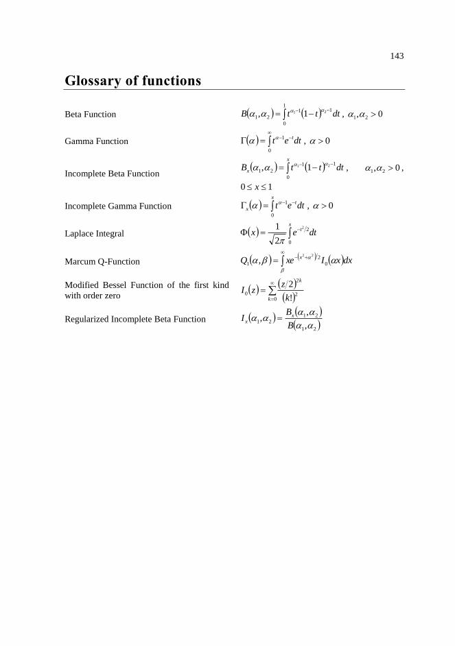
143
Glossary of functions
Beta Function
1
0
11
2121 1, dtttB
, 0, 21
Gamma Function
0
1 dtet t , 0
Incomplete Beta Function
x
x dtttB0
11
2121 1,
, 0, 21 ,
10 x
Incomplete Gamma Function
xt
x dtet0
1 , 0
Laplace Integral
xt dtex
0
22
2
1
Marcum Q-Function
dxxIxeQ x
0
2
1
22
,
Modified Bessel Function of the first kind
with order zero
0
2
2
0!
2
k
k
k
zzI
Regularized Incomplete Beta Function 21
2121
,
,,
B
BI x
x


145
Bibliography
[Adrianova 1995] L. Ya. Adrianova (1995), “Introduction to linear systems of differential
equations”, American Mathematical Society, Providence, RI.
[Al-Mohy 2009] A. H. Al-Mohy, N. J. Higham (2009), “A new scaling and squaring
algorithm for the matrix exponential”, SIAM Journal on Matrix
Analysis and Applications, vol. 31 (3), pp. 970-989.
[Bécoulet 2008] M. Bécoulet et al (2008), “Numerical study of the resonant magnetic
perturbations for Type I edge localized modes control in ITER”,
Nuclear Fusion, vol. 48 (2), 024003.
[Bellu 2007] G. Bellu, M. P. Saccomani, S. Audoly, L. D’Angiò (2007), “DAISY: A
new software tool to test global identifiability of biological and
physiological systems”, Computer Methods and Programs in
Biomedicine, vol. 88 (1), pp. 52-61.
[Benettin 1980a] G. Benettin, L. Galgani, A. Giorgilli, J. M. Strelcyn (1980), “Lyapunov
characteristic exponents for smooth dynamical systems and for
Hamiltonian systems; a method for computing all of them. Part 1:
Theory”, Meccanica, vol. 15 (1), pp. 9-20.
[Benettin 1980b] G. Benettin, L. Galgani, A. Giorgilli, J. M. Strelcyn (1980), “Lyapunov
characteristic exponents for smooth dynamical systems and for
Hamiltonian systems; a method for computing all of them. Part 2:
Numerical application”, Meccanica, vol. 15 (1), pp. 21-30.
[Bishop 1996] C. M. Bishop (1996), “Neural networks for pattern recognition”,
Oxford University Press, New York.
[Blanes 2008] S. Blanes, F. Casas, J. A. Oteo, J. Ros (2009), “The Magnus expansion
and some of its applications”, Physics Reports, vol. 470 (5-6), pp. 151-
238.
[Bomze 1999] I. M. Bomze, M. Budinich, P. M. Pardalos, M. Pelillo (1999), “The
maximum clique problem”, Handbook of Combinatorial Optimization,
Kluwer Academic Publishers, vol. 4, pp. 1-74.
[Box 1970] G. E. P. Box, G. M. Jenkins (1970), “Time series analysis: forecasting
and control”, Holden-Day, San Francisco, California.
[Cafagna 2003] D. Cafagna, G. Grassi (2003), “New 3D-scroll attractors in
hyperchaotic Chua’s circuits forming a ring”, International Journal of
Bifurcation and Chaos, vol. 13 (10), pp. 2889-2903.

146
[Camplani 2009] M. Camplani, B. Cannas, P. Carboni (2009), “Dynamic behaviour of
two coupled Lorenz systems”, Analysis and Control of Chaotic
Systems, Proceedings of 2nd IFAC Conference on, London, UK, June
22nd—24th, 2009, vol. 2 (1), pp. 62-66.
[Canik 2010] J.M. Canik et al (2010), “Progress in the development of ELM pace-
making with non-axisymmetric magnetic perturbations in NSTX”,
Nuclear Fusion, vol. 50 (6), 064016.
[Cannas 2002] B. Cannas, S. Cincotti (2002), “Hyperchaotic behaviour of two bi-
directionally coupled Chua’s circuits”, International Journal of Circuit
Theory and Applications, vol. 30 (6), pp. 625-637.
[Chen 2002] W. K. Chen (2002), “The circuits and filters handbook, 2nd
edition”,
CRC Press.
[Chialina 1994] S. Chialina, M. Hasler, A. Premoli (1994), “Fast and accurate
calculation of Lyapunov Exponents for piecewise-linear systems”,
International Journal of Bifurcations and Chaos, vol. 4 (1), pp. 127-
136.
[Cincotti 2007] S. Cincotti, A. Teglio (2007), “A systematic approach to bi-
directionally nonlinearly coupled systems design for the generation of
complex dynamical behaviours”, Circuits and Systems I: Regular
Papers, IEEE Transactions on, vol. 54 (6), pp. 1340-1347.
[Cybenko 1989] G. Cybenko (1989), “Approximation by superpositions of a sigmoidal
function”, Mathematics of Control, Signals and Systems, vol. 2 (4), pp.
303-314.
[Davis 2002] J. C. Davis (2002), “Statistics and data analysis in geology”, John
Wiley & Sons, Inc., New York.
[Dieci 1997] L. Dieci, R. D. Russell, and E. S. Van Vleck (1997), “On the
Computation of Lyapunov Exponents for Continuous Dynamical
Systems”, SIAM Journal on Numerical Analysis, vol. 34 (1), pp. 402-
423.
[Donoho 1994] D. L. Donoho, I. M. Johnstone (1994), “Ideal Spatial Adaptation by
Wavelet Shrinkage”, Biometrika, 81 (3), pp. 425-455.
[Dowdy 2004] S. Dowdy, S. Weardon, D. Chilko (2004), “Statistics for research”,
John Wiley & Sons, Inc., Hoboken, New Jersey.
[Duro 2009] N. Duro, R. Dormido, J. Vega, S. Dormido-Canto, G. Farias, J.
Sánchez, H. Vargas, A. Murari, JET-EFDA Contributors (2009),
“Automated recognition system for ELM classification in JET”,
Fusion Engineering and Design, vol. 84 (2-6), pp. 712-715.
147
[Eckmann 1985] J. P. Eckmann, D. Ruelle (1985), “Ergodic theory of chaos and strange
attractors”, Reviews of Modern Physics, 57 (3), pp. 617-656.
[Eckmann 1986] J. P. Eckmann, S. Oliffson Kamphorst, D. Ruelle, S. Ciliberto (1986),
“Liapunov exponents from time series”, Physical Review A, vol. 34
(6), pp. 4971-4979.
[Elman 1990] J. L. Elman (1990), “Finding structure in time”, Cognitive Science, vol.
14 (2), pp. 179-211.
[Elwakil 2006] A. S. Elwakil, S. Ozoguz (2006), “On the generation of higher order
chaotic oscillators via passive coupling of two identical or nonidentical
sinusoidal oscillators”, Circuits and Systems I: Regular Papers, IEEE
Transactions on, vol. 53 (7), pp. 1521-1532.
[Feller 1968] W. Feller (1968), “An introduction to probability theory and its
applications”, John Wiley & Sons, Inc., New York.
[Fliess 1993] M. Fliess, S. T. Glad (1993), “An algebraic approach to linear and
nonlinear control”, Essays on Control: Perspectives in the Theory and
Its Applications, Birkhäuser Boston, vol. 14, pp. 223-267.
[Forsman 1992] K. Forsman (1992), “Constructive commutative algebra in nonlinear
control theory”, Ph. D dissertation, Linkoping Studies in Science and
Technology, Department of Electrical Engineering, Linkoping
University, Linkoping, Sweden.
[Gao 2010] J. Gao, H. Sultan, J. Hu, W. W. Tung (2010), “Denoising nonlinear
time series by adaptive filtering and wavelet shrinkage: a comparison”,
Signal Processing Letters, IEEE, vol. 17 (3), pp. 237-240.
[Grassi 2009] G. Grassi, F. L. Severance, D. A. Miller (2009), “Multi-wing
hyperchaotic attractors from coupled Lorenz systems”, Chaos, Solitons
and Fractals, vol. 41 (1), pp. 284-291.
[Han 2006] M. Han, Y. Liu, J. Xi, W. Guo (2006), “Noise smoothing for nonlinear
time series using wavelet soft threshold”, Signal Processing Letters,
IEEE, vol. 14 (1), pp. 62-65.
[Han 2009] M. Han, Y. Liu (2009), “Noise reduction method for chaotic signals
based on dual-wavelet and spatial correlation”, Expert Systems with
Applications, vol. 36 (6), pp. 10060-10067.
[Harary 1957] F. Harary, I. C. Ross (1957), “A procedure for clique detection using
the group matrix”, Sociometry, vol. 20 (3), pp. 205-215.
[Hegger 1999] R. Hegger, H. Kantz, T. Schreiber (1999), “Practical implementation of
nonlinear time series methods: the TISEAN package”, Chaos, vol. 9
(2), pp. 413-435.

148
[Hertz 1991] J. Hertz, A. Krogh, R. G. Palmer (1991), “Introduction to the Theory
of Neural Computation”, Addison-Wesley.
[Higham 2002] N. J. Higham (2002), “Accuracy and stability of numerical
algorithms”, SIAM. http://www.ma.man.ac.uk/_higham/mftoolbox.
[Higham 2005] N. J. Higham (2005), “The scaling and squaring method for the matrix
exponential revisited”, SIAM Journal on Matrix Analysis and
Applications, vol. 26 (4), pp. 1179-1193.
[Hopfield 1982] J. J. Hopfield (1982), “Neural networks and physical systems with
emergent collective computational abilities”, Proceedings of the
National Academy of Sciences of the United States of America, vol. 79
(8), pp. 2554-2558.
[Hu 2011] G. Hu (2011), “Hyperchaos of higher order and its circuit
implementation”, International Journal of Circuit Theory and
Applications, vol. 39 (1), pp. 79-89.
[Huang 1996] A. S. Huang, L. Pivka, C. W. Wu, M. Franz (1996), “Chua’s equation
with cubic nonlinearity”, International Journal of Bifurcation and
Chaos, vol. 6 (12a), pp. 2175-2222.
[Hurst 1951] H. E. Hurst (1951), “Long-term storage of reservoirs: an experimental
study”, Transactions of the American society of civil engineers, vol.
116, pp. 770–799.
[ITER 1999] ITER Physics Expert Group on Confinement and Transport et al.
(1999), “Chapter 2: Plasma confinement and transport”, Nuclear
Fusion, vol. 39 (12), pp. 2175-2249.
[Kantz 2004] H. Kantz, T. Schreiber (2004), “Nonlinear time series analysis”,
Cambridge University Press, Cambridge.
[Kapitaniak 1994] T. Kapitaniak, L. O. Chua, G. Zhong (1994), “Experimental
hyperchaos in coupled Chua’s circuits”, Circuits and Systems I:
Fundamental Theory and Applications, IEEE Transactions on, vol. 41
(7), pp. 499-503.
[Kohonen 1990] T. Kohonen (1990), “The self-organizing map”, Proceedings of the
IEEE, vol. 78 (9), pp. 1464-1480.
[Kriesel 2007] D. Kriesel (2007), “A brief introduction to neural networks”, available
at http://www.dkriesel.com.
[Lang 2004] P. Lang et al (2004), “ELM pace making and mitigation by pellet
injection in ASDEX Upgrade”, Nuclear Fusion, vol. 44 (5), pp. 665-
677.

149
[LET] http://www.mathworks.cn/matlabcentral/fileexchange/233-let
[Li 2008] Q. Li, X. S. Yang (2008), “Hyperchaos from two coupled Wien-bridge
oscillators”, International Journal of Circuit Theory and Applications,
vol. 36 (1), pp. 19-29.
[Li 2011] Y. Li, X. Liu, G. Chen, X. Liao (2011), “A new hyperchaotic Lorenz-
type system: Generation, analysis, and implementation”, International
Journal of Circuit Theory and Applications, vol. 39 (8), pp. 865-879.
[Ljung 1994] L. Ljung, S. T. Glad (1994), “On global identifiability for arbitrary
model parameterizations”, Automatica, vol. 30 (2), pp. 265-276.
[Ljung 1999] L. Ljung (1999), “System Identification: Theory for the User”, Prentice
Hall.
[Lo 2001] A. W. Lo (2001), “A Non-Random Walk Down Wall Street”,
Princeton University Press.
[Lorenz 1963] E. N. Lorenz (1963), “Deterministic nonperiodic flow”, Journal of
Atmospheric Sciences, vol. 20 (2), pp.130-141.
[Lorenzo 1996] M. N. Lorenzo, I. P. Marino, V. Perez-Munuzuri, M. A. Matias, V.
Perez-Villar (1996), “Synchronization waves in arrays of driven
chaotic systems”, Physical Review E, vol. 54 (4), pp. 3094-3097.
[Ma 2002] X. Ma, C. Zhou, I. J. Kemp (2002), “Automated wavelet selection and
thresholding for PD detection”, Electrical Insulation Magazine, IEEE,
vol. 18 (2), pp. 37-45.
[Massey 1951] F. J. Massey (1951), "The Kolmogorov-Smirnov Test for Goodness of
Fit", Journal of the American Statistical Association, vol. 46 (253), pp.
68–78.
[Matias 1997] M. A. Matias, J. Guemez, V. Perez-Munuzuri, I. P. Marino, M. N.
Lorenzo (1997), “Size instabilities in rings of chaotic synchronized
systems”, Europhysics Letters, vol. 37 (6), pp. 379-384.
[Matsumoto 1985] T. Matsumoto, L. Chua, M. Komuro (1985), “The double scroll”,
Circuits and Systems, IEEE Transactions on, vol. 33 (8), pp. 797–818.
[Matsumoto 1986] T. Matsumoto, L. Chua, K. Kobayashi (1986), “Hyper chaos:
laboratory experiment and numerical confirmation”, Circuits and
Systems, IEEE Transactions on, vol. 33 (11), pp. 1143–1147.
[McCulloch 1943] W. S. McCulloch, W. Pitts (1943), “A logical calculus of the ideas
immanent in nervous activity”, The Bulletin of Mathematical
Biophysics, vol. 5 (4), pp. 115-133.

150
[Mohammadi 2009] S. Mohammadi (2009), "LYAPROSEN: MATLAB function to
calculate Lyapunov exponent", Statistical Software Components
T741502, Boston College Department of Economics.
[Parker 1986] T. S. Parker, L. O. Chua (1986), “Efficient solution of the variational
equation for piecewise-linear differential equations”, International
Journal of Circuit Theory and Applications, vol. 14 (4), pp. 305-314.
[Parker 1989] T. S. Parker, L. O. Chua (1989), “Practical numerical algorithms for
chaotic systems”, Springer-Verlag, New York.
[Peters 1994] E. E. Peters (1994), “Fractal Market Analysis: Applying Chaos Theory
to Investment and Economics”, John Wiley & Sons, New York.
[Polyanin 2007] A. D. Polyanin, A. V. Manzhirov (2007), “Handbook of mathematics
for engineers and scientists”, Chapman & Hall/ CRC.
[Ritt 1950] J. F. Ritt (1950), “Differential Algebra”, Colloquium Publications,
American Mathematical Society, Providence, Rhode Island, vol. 33.
[Rosenblatt 1958] F. Rosenblatt (1958), “The perceptron: a probabilistic model for
information storage and organization in the brain”, Psychological
Review, vol. 65 (6), pp. 386-408.
[Rosenstein 1993] M. T. Rosenstein, J. J. Collins, C. J. De Luca (1993), “A practical
method for calculating largest Lyapunov exponents from small data
sets”, Physica D, vol. 65 (1-2), pp. 117-134.
[Rossler 1979] O. E. Rossler (1979), “An equation for hyperchaos”, Physics Letters A,
vol. 71 (2-3), pp.155-157.
[Rumelhart 1986] D. E. Rumelhart, G. E. Hinton, R. J. Williams (1986), “Learning
representations by back-propagating errors”, Nature, vol. 323 (6088),
pp. 533-536.
[Sachs 1984] L. Sachs (1984), “Applied Statistics: A Handbook of Techniques”,
Springer-Verlag, New York.
[Sanchez 2000] E. Sanchez, M. A. Matias, V. Perez-Munuzuri (2000), “Chaotic
synchronization in small assemblies of driven Chua’s circuits”,
Circuits and Systems I: Fundamental Theory and Applications, IEEE
Transactions on, vol. 47 (5), pp. 644-654.
[Sano 1985] M. Sano, Y. Sawada (1985), “Measurement of the Lyapunov spectrum
from a chaotic time series”, Physical Review Letters, vol. 55 (10), pp.
1082-1085.
[Sauer 1991] T. Sauer, J. Yorke, M. Casdagli (1991), “Embedology”, Journal of
Statistical Physics, vol. 65 (3-4), pp. 579-616.
151
[Shimada 1979] I. Shimada, T. Nagashima (1979), “A numerical approach to ergodic
problem of dissipative dynamical systems”, Progress of Theoretical
Physycs, vol. 61 (6), pp. 1605-1616.
[Staszewski 1999] W. J. Staszewski, K. Worden (1999), “Wavelet analysis of time-series:
coherent structures, chaos and noise”, International Journal of
Bifurcation and Chaos, vol. 9 (3), pp. 455-471.
[Stone 1974] M. Stone (1974), “Cross-validatory choice and assessment of statistical
predictions”, Journal of the Royal Statistical Society, Series B
(Methodological), vol. 36 (2), pp. 111-147.
[Stone 1978] M. Stone (1978), “Cross-validation: a review”, Series Statistics, vol. 9
(1), pp. 127-139.
[Storace 2005] M. Storace, O. De Feo (2005), “PWL approximation of nonlinear
dynamical systems, part I: structural stability”, Journal of Physics:
Conference Series, vol. 22, pp. 208-221.
[Strogatz 1994] S. H. Strogatz, D. E. Herbert (1994), “Nonlinear dynamics and chaos:
with applications to physics, biology, chemistry, and engineering”,
Perseus Books, Reading, MA.
[Suttrop 2000] W. Suttrop (2000), “The physics of large and small edge localized
modes”, Plasma Physics and Controlled Fusion, vol. 42 (5A), pp. A1-
A14.
[Suykens 1997] J. A. K. Suykens, L. O. Chua (1997), “n-double scroll hypercubes in 1-
D CNNs”, International Journal of Bifurcation and Chaos, vol. 7 (8),
1873-1885.
[Suzuki 1994] T. Suzuki, T. Saito (1994), “On fundamental bifurcations from a
hysteresis hyperchaos generator”, Circuits and Systems I: Fundamental
Theory and Applications, IEEE Transactions on, vol. 41 (12), pp. 876–
884.
[Takens 1981] F. Takens (1981), “Detecting Strange Attractors in Turbulence”,
Dynamical Systems and Turbulence, Warwick, 1980, Lecture Notes in
Mathematics, vol. 898, pp. 366-381.
[Wahba 1975] G. Wahba, S. Wold (1975), “A completely automatic French curve:
fitting spline functions by cross-validation”, Communications in
Statistics, vol. 4 (1), pp. 1-17.
[Wesson 2004] J. Wesson et al (2004), “Tokamaks”, Oxford University Press, New
York.
[Widrow 1960] B. Widrow, M. E. Hoff (1960), “Adaptive switching circuits”, IRE
WESCON Convention Record, vol. 4, pp. 96-104.

152
[Wilson 2008] H. Wilson (2008), “Edge localized modes in tokamaks”, Fusion
Science and Technology, vol. 53 (2T), pp. 161-169.
[Wolf 1985] A. Wolf, J. B. Swift, H. L. Swinney, J. A. Vastano (1985),
“Determining Lyapunov exponents from a time series”, Physica D:
Nonlinear Phenomena, vol. 16 (3), pp. 285-317.
[Wornell 1992] G. W. Wornell, A. V. Oppenheim (1992), “Wavelet-based
representations for a class of self-similar signals with application to
fractal modulation”, Information Theory, IEEE Transactions on, vol.
38 (2), pp. 785-800.
[Zedda 2008] M. K. Zedda, M. Camplani, B. Cannas, A. Fanni, P. Sonato, E. Solano,
JET-EFDA contributors (2008), “Dynamic behaviour of type I Edge
Localized Modes in the JET”, The 35th EPS Conference on Plasma
Physics and Controlled Fusion, 09 - 13 June 2008, Hersonisson, Crete,
Greece, vol. 32D, P-4.070.
[Zhang 2010] C. Zhang, S. Yu (2010), “On constructing complex grid multi-wing
hyperchaotic system: Theoretical design and circuit implementation”,
International Journal of Circuit Theory and Applications, vol. 40 (12).
[Zohm 1996] H. Zohm (1996), “Edge localized modes”, Plasma Physics and
Controlled Fusion, vol. 38 (2), pp. 105-128.
153
List of publications related to the thesis
Journal papers
B. Cannas, F. Pisano (2012), “Effect of a particular coupling on the dynamic behavior of
nonlinear systems”, International Journal of Circuit Theory and Applications, doi:
10.1002/cta.1867. Relation to Chapter 8.
Conference papers
B. Cannas, F. Pisano (2011), "A fast algorithm for Lyapunov exponents calculation in
piecewise linear systems", AIP Conference Proceedings of 9th International Conference of
Numerical Analysis and Applied Mathematics (ICNAAM 2011), Halkidiki, Greece, 19-25
September 2011, vol. 1389, pp. 1844-1847. Relation to Chapter 7.
B. Cannas, F. Pisano, A. Montisci (2013), "Identification of chaotic systems by neural
networks", Proceedings of the 4th International Interdisciplinary Chaos Symposium on
Chaos and Complex Systems (CCS 2012), Antalya, Turkey, 29 April – 1 May 2012,
publication due on March 31, 2013. Relation to Chapter 9.
B. Cannas, F. Pisano (2013), "A piecewise linear approximation method for the evaluation
of Lyapunov Exponents of polynomial nonlinear systems", Proceedings of the 4th
International Interdisciplinary Chaos Symposium on Chaos and Complex Systems (CCS
2012), Antalya, Turkey, 29 April – 1 May 2012, publication due on March 31, 2013.
Relation to Chapter 7.
B. Cannas, A. Murari, F. Pisano (2013), “Time series denoising based on wavelet
decomposition and cross-correlation between the residuals and the denoised signal”,
Proceedings of the 10th IASTED International Conference on Signal Processing, Pattern
Recognition and Applications (SPPRA 2013), Innsbruck, Austria, 12-14 February 2013,
accepted. Relation to Chapter 10.