PFI, Trondheim, October 24-26, 2012

1Department of Energy and Process Engineering, NTNU

2Centro Interdipartimentale di Fluidodinamica e Idraulica, University of Udine

L. Zhao1, C. Marchioli2, H. Andersson1

Joint 4th SIG43 –FP1005 Workshop on

Fiber Suspension Flow Modelling

Slip Velocity of Rigid Fibers

in Wall-Bounded Turbulence

Motivation of the Study:Why are we looking at the slip

velocity?Slip velocity is a crucial variable in:

1. Euler-Lagrange simulations:

• One-way coupling: determines the drag experienced by fibers

• Two-way coupling: determinesreaction force from fibers on fluid

2. Two-fluid modeling of particle-laden flows

• Modeling SGS fiber dynamics in LES flow fields

• Crossing trajectory effects on time decorrelation tensor of u

v

u

u: fluid velocity “seen”

v: fiber velocity

∆u=u-v: slip velocity

Aim of this study: statistical characterization of ∆u at varying fiber inertia and elongation

Examples: flow of air at 1.8 m/s in a 4 cm high channel

Pseudo-Spectral method: Fourier modes in x and y, Chebyschev modes in z.

Methodology - Carrier Fluid

flow of water at 3.8 m/s in a 0.5 cm high channel

DNS of turbulent channel flow @ Ret=ut h/n=150, 180, 300

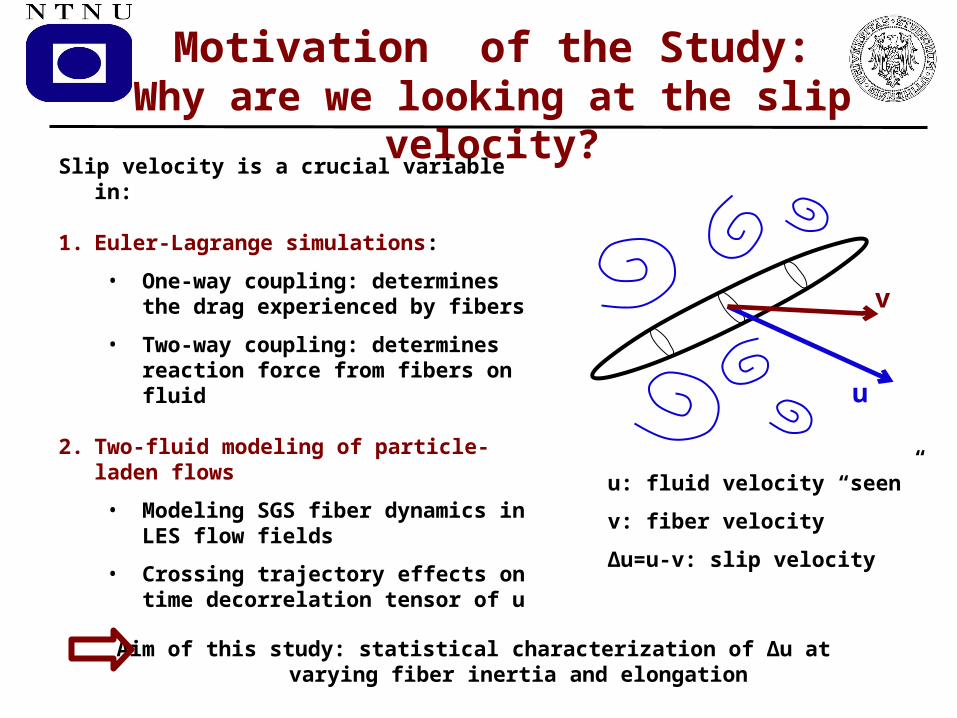
Fibers are modelled as prolate ellipsoidal particles.

Lagrangian particle tracking.

Simplifying assumptions: dilute flow, one-way coupling, Stokes flow (ReP<1 ), pointwise particles (particle size is smaller than the smallest flow scale).

Periodicity in x ed y, elastic rebound at the wall and conservation of angular momentum.

200,000 fibers tracked, random initial position and orientation, linear and angular velocities equal to those of the fluid at fiber’s location.

Methodology - Fibers

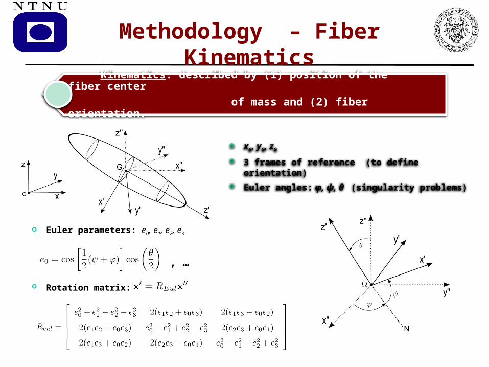
Kinematics: described by (1) position of the fiber center of mass and (2) fiber orientation.

xG, yG, zG

3 frames of reference (to define orientation) Euler angles: φ, ψ, θ (singularity problems)

Euler parameters: e0, e1, e2, e3

Rotation matrix:

, …

Methodology – Fiber Kinematics

Euler Equations: (2nd cardinal law)

(in the particle frame)

Rotational dynamics: Euler equations with Jeffery moments.

Jeffery moments:

Aspect Ratio

Hence: Euler equations with Jeffery

couples

e0, e1, e2, e3

(Euler parameters)

),,,( 3210 eeeeRR euleul

(Jeffery, 1922)

Methodology – Fiber Dynamics

Translational Dynamics: hydrodynamic resistance (Brenner, 1963).

First cardinal law:

Brenner’s law: (form drag and

skin drag)

(in the fiber frame)

In the inertial (Eulerian) frame: Resistance

Tensor

,

Once fiber orientation is known, fiber translational motion can be computed!

(inertia and drag only!!)

(via numerical integration)

Methodology – Fiber Dynamics

Stokes number: (chosen values: t+=1, 5, 30, 100) F

PSt

Specific density:

The physics of turbulent fiber dispersionis determined by a small set of parameters

Input parameters: S, τ , λ+

τ >> 1: large inertia (“stones”)

τ << 1 : small inertia (tracers)

τ ~ 1 : preferential (selective)

response to flow structures

+

+

+

Relevant Parameters and Summary of the

Simulations

Aspect ratio: (chosen values: l=1.001, 3, 10, 50) a

b

F

PS

“Cartoon” offiber ’s elongation

l=1.001 (spherical particle)

l=3

l=10

l=50 (elongated “spaghetti-like” fiber)

Top view: fibers accumulate in near-wall fluid Low-Speed Streaks (LSS)

Results - Non-Homogeneity ofNear-Wall Fiber Preferential

Distribution

Slip velocity at fiber position:

Sample snapshot for t+=30, l=50 fibers

Results - Using Slip Velocity to Analyze

Fiber Accumulation in LSS

The influence of λ is not dramatic: only a change in thepeak values is observed (no PDF shape change)

Effect of fiber elongation on conditioned PDF(uf’) – St=30

Positive slip

Negative slip

l=1l=3l=10l=50

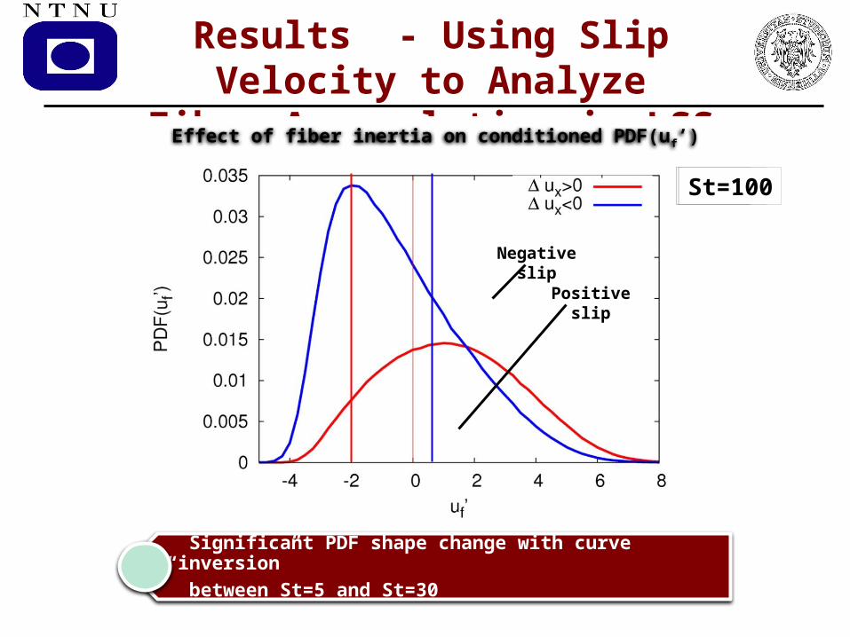
Results - Using Slip Velocity to Analyze

Fiber Accumulation in LSS

Significant PDF shape change with curve “inversion” between St=5 and St=30

Effect of fiber inertia on conditioned PDF(uf’)

Positive slip

Negative slip

St=1St=5St=30St=100

Results - Streamwise Slip Velocity:

Mean and RMS valuesSt=1

St=30

Mean RMS

Mean RMS

Results - Streamwise Slip Velocity:

Mean and RMS valuesSt=5

St=100

Mean RMS

Mean RMS

Results - Wall-Normal Slip Velocity:

Mean and RMS valuesSt=1

St=30

Mean RMS

Mean RMS

Conclusions ……and Future Developments

Slip velocity is a useful measure of fibers-turbulence interaction in wall-bounded flows: its statistical characterization provides useful indications for modeling turbulent fiber dispersion

Slip velocity statistics depend both on fiber elongation (quantitatively) and fiber inertia (also qualitatively!)

RMS exceeds the corresponding mean value by roughly 3 to 5 times: the instantaneous slip velocity may thus frequently change sign

Simulate more values of St, λ and Re

Evaluate slip spin statistics

l

Mean slip spin for the St=30fibers in the Re=150 flow(spanwise component)