Petrophysical seismic inversion conditioned to well-log ...Petrophysical seismic inversion conditioned to well-log data: Methods and application to a gas reservoir Miguel Bosch1, Carla

Pa

MJ

gsitpgpacwfi

@

c

©

GEOPHYSICS, VOL. 74, NO. 2 �MARCH-APRIL 2009�; P. O1–O15, 11 FIGS.10.1190/1.3043796

etrophysical seismic inversion conditioned to well-log data: Methodsnd application to a gas reservoir

iguel Bosch1, Carla Carvajal2, Juan Rodrigues1, Astrid Torres2, Milagrosa Aldana3, andesús Sierra4

stWddtawwrilpp

ABSTRACT

Hydrocarbon reservoirs are characterized by seismic, well-log, and petrophysical information, which is dissimilar in spatialdistribution, scale, and relationship to reservoir properties. Wecombine this diverse information in a unified inverse-problemformulation using a multiproperty, multiscale model, linkingproperties statistically by petrophysical relationships and condi-tioning them to well-log data. Two approaches help us: �1� Mark-ov-chain Monte Carlo sampling, which generates many reservoirrealizations for estimating medium properties and posterior mar-ginal probabilities, and �2� optimization with a least-squares iter-ative technique to obtain the most probable model configuration.Our petrophysical model, applied to near-vertical-anglestacked

dr

tdrenspd1�i

ved 17 Sion La

n Labor

zuela. Egs-sc.co

O1

Downloaded 13 Apr 2009 to 200.44.243.220. Redistribution subject to

eismic data and well-log data from a gas reservoir, includes a de-erministic component, based on a combination of Wyllie and

ood relationships calibrated with the well-log data, and a ran-om component, based on the statistical characterization of theeviations of well-log data from the petrophysical transform. Athe petrophysical level, the effects of porosity and saturation oncoustic impedance are coupled; conditioning the inversion toell-log data helps resolve this ambiguity. The combination ofell logs, petrophysics, and seismic inversion builds on the cor-

esponding strengths of each type of information, jointly improv-ng �1� cross resolution of reservoir properties, �2� vertical reso-ution of property fields, �3� compliance to the smooth trend ofroperty fields, and �4� agreement with well-log data at wellositions.

INTRODUCTION

The 3D characterization of hydrocarbon reservoirs requires inte-rating information across medium properties at different spatialcales and distributions: �1� high-resolution well-log information atrregularly distributed well paths, �2� uniformly sampled informa-ion from 3D seismic data with low vertical resolution, �3� petro-hysical information relating reservoir properties and scales, and �4�eostatistical information relating property fields in space. Commonrocedures rely on stepwise processing of the different types of datand information �seismic, well log, petrophysical, and geostatisti-al� and their combination in various work flows. The goal of ourork is to describe a method to integrate this information into a uni-ed inversion scheme, accounting for nonlinear relations across me-

Manuscript received by the Editor 5 March 2008; revised manuscript recei1Universidad Central of Venezuela, Geophysical Simulation and Inversucv.ve.2Universidad Central of Venezuela, Geophysical Simulation and Inversio

as, Venezuela.3Universidad Simón Bolivar, Department of Earth Sciences, Caracas, Vene4IGS Services and Consulting, Caracas, Venezuela. E-mail: jesus.sierra@i2009 Society of Exploration Geophysicists.All rights reserved.

ium properties and data as well as the combination of uncertaintieselated to the various information components.

The combination of well-log data and seismic information for es-imating reservoir and elastic medium properties has motivated theevelopment of different techniques. In Doyen �1988�, well-log po-osities are extrapolated by correlation with the acoustic impedancestimated from seismic data, using the well-known cokriging tech-ique. An additional step in integrating seismic data within geo-tatistical methods is described by Haas and Dubrule �1994�, whoropose a method to generate acoustic impedance realizations con-itioned to the well-log data and seismic stacked data simulated byD convolution of the model reflectivity. Also, Torres-Verdin et al.1999� focus on the problem of generating realizations of acousticmpedance and discrete facies types jointly honoring stacked seis-

eptember 2008; published online 4 February 2009.boratory, Engineering Faculty, Caracas, Venezuela. E-mail: miguel.bosch

atory, and Universidad Simón Bolivar, Department of Earth Sciences, Cara-

-mail: [email protected].

SEG license or copyright; see Terms of Use at http://segdl.org/

mgejGus

vreog

cppeBsiraappmlaprfint

optmmcpdm�a

sdbgsfbE1paslaf

ttbsaeaiea

bfmscv

mpt�atdr

Flri

O2 Bosch et al.

ic data and well logs using a simulated annealing technique. Inte-ration of well-log data and seismic data partially stacked at differ-nt incidence angle ranges is described by Contreras et al. �2005� foroint estimation of elastic medium parameters and facies types. Inonzalez et al. �2008�, facies types also are related with seismic datasing a multipoint geostatistical model that honors spatial well con-traints.

We can circumscribe these works to the field of geostatistical in-ersion of seismic data. The advantages of geostatistical inversionelated to plain geophysical inversion are manifold: estimated prop-rty fields match well-log data at well location, seismic data are hon-red, and field resolution increases along the well direction in the re-ion within the range of spatial property correlation.

Effort has been directed to integrate petrophysical and geophysi-al inversion within a common inference formulation. In this ap-roach, the seismic data are inverted under the constraint of a petro-hysical model and prior information; the result is a joint estimate oflastic and reservoir �e.g., porosity, facies, fluid� properties. Inosch �2004�, a statistical formulation for the joint inversion is de-

cribed and numerical examples are presented for the case of invert-ng short-offset seismic data to estimate acoustic impedance and po-osity. The relation between impedance and porosity is embodied inpetrophysical mixed model �deterministic mean and random devi-tions� calibrated to well-log data; an optimization method is used toroduce a linear system of equations for the joint porosity and im-edance model updates. Bosch et al. �2007� describe a similar for-ulation to solve the inference problem with a sampling Monte Car-

o approach, providing an application to a field case. Also, Spikes etl. �2007� focus on constraining a seismic inversion with a petro-hysical model calibrated to well-log data and estimating elastic andeservoir parameters from two constant-angle stacks, showing aeld case. Larsen et al. �2006�, Buland and Omre �2006�, and Gun-ing and Glinski �2007� describe similar methods illustrated by syn-hetic tests.

igure 1. Model parameters and data involved in the inference prob-em—information components and their relations. Thin black ar-ows indicate the forward-modeling sense. Thick arrows indicate thenverse sense.


We can group these works in the field of petrophysical inversionf seismic data. The advantages of petrophysical inversion com-ared to plain seismic inversion are also manifold: reservoir proper-ies are estimated in addition to elastic properties, relations across

edium properties honor the petrophysical model, and prior infor-ation constraining the reservoir properties holds. Other ways to

ombine seismic and petrophysical information follow a two-steprocess: �1� calculating seismic attributes or inverting the seismicata and �2� using these results within a petrophysical statisticalodel to estimate reservoir parameters. Work by Eidsvik et al.

2004�, Bachrach �2006�, Mukerji et al. �2001�, Saltzer et al. �2005�,nd Sengupta and Bachrach �2007� is based on this approach.

Our work extends the method of petrophysical inversion de-cribed by Bosch �2004� and Bosch et al. �2007� to include well-logata constrained on the basis of a geostatistical model, combiningenefits of the geostatistical and petrophysical approaches and inte-rating surface seismic data, well-log data, petrophysics, and geo-tatistics. We parameterize the model in two scales to address the dif-erent resolution of well logs and seismic data, with a scale relationetween them based on petrophysical change of support transforms.ffective medium theory �Backus, 1962; Schoenberg and Muir,989� describes averaging functions to obtain the elastic mediumarameters at seismic resolution from the corresponding parameterst finer resolution; it also encompasses the full anisotropic elastictiffness tensor parameters. Impedances, for instance, commonly areower at seismic scale than the corresponding impedances measuredt well-log scale. Ray theory, on the other hand, provides averagingunctions for the properties, assuming high-frequency propagation.

The two formulations correspond to the upper and lower limits ofhe ratio between the wavelength and the characteristic thickness ofhe strata. Behavior at intermediate ratios is bounded approximatelyy the effective media and ray-theory results, depending on factorsuch as the statistical spatial characterization of the heterogeneitiesnd the actual frequency composition of the signal as shown by mod-ling and laboratory tests �Mukerji, 1995; Grechka, 2003; Stovasnd Arntsen, 2006�. In many practical applications to reservoirs, anntermediate recipe combining the two bounds is recommended �Riot al., 1996�. Here, we use an upscaling formulation of the imped-nce that lies between these two limits.

We describe our methods, characterize the well-log data to cali-rate our petrophysical and geostatistical models, and apply two dif-erent inversion techniques — sampling and optimization — to seis-ic data from a gas reservoir area. For comparison, we show the re-

ults obtained from the seismic petrophysical inversion with no wellonditioning, the plain geostatistical estimation, and the seismic in-ersion conditioned by the well-log data.

THEORY AND METHOD

The joint model parameter array is a composition, m � �mgeo,

elas�, of parameters describing the reservoir property fields mgeo andarameters describing the elastic-property fields melas. In addition,he elastic properties are described at two different vertical scales:1� high-resolution parameters linked with the well-log informationnd �2� low-resolution parameters according to the vertical resolu-ion of the seismic data. Figure 1 describes the model parameters, theata subspaces, the information involved in the problem, and theirelations.


S

posf

Ttcletmufsdevs

etucClob

wvls�

vst�

mtsmbad

wt

cs

waf�c

Tt

ivlf�t

wfttlc

popstsaa

taamdi

P

aibn

Integrated inversion of reservoir data O3

tatistical formulation

The knowledge about medium parameters is described with arobability density function �PDF� that combines the different typesf information and data considered. The combined probability den-ity is given by the product of three factors that cast the types of in-ormation included in our problem �Bosch, 1999�:

�1�he PDF �geo�mgeo� describes the prior geostatistical information in

he reservoir property fields, including the well-data constraints. Theonditional probability density ��melas�mgeo� is a petrophysical like-ihood function, based on the petrophysical model that predicts thelastic properties from the reservoir properties. In addition, this fac-or embodies geostatistical constraints of the elastic properties; it

easures the probability of the elastic-property fields given a partic-lar reservoir field configuration and well-log measurements. Theactor Lseis�melas� is the geophysical likelihood function that mea-ures the proximity between the observed and calculated seismicata. It depends on the elastic-property field parameters. We modelach of the factors of the combined probability density with multi-ariate parametric functions and implement solution methods byampling and optimization approaches.

As common in geostatistical formulation, property fields are mod-led as a multidimensional random variable, with components beinghe values of the properties at a given set of points in the medium vol-me. We model the reservoir-property fields, prior to the well-logonstraints, with a Gaussian multivariate prior probability density.onditioning the Gaussian property field to known values of corre-

ated properties at a given set of points �here, the well-log estimatesf the property field� results in a random Gaussian field with proba-ility density

�geo�mgeo� � c2 exp��1/2�mgeo � mgeo krig�T

� Cgeo krig�1 �mgeo � mgeo krig�� , �2�

here mgeo krig and Cgeo krig are the simple cokriging estimate and co-ariance that result from the geostatistical interpolation of the well-og data. For a review on geostatistical estimation and conditionalimulation, see Isaaks and Srivastava �1989�, Chiles and Delfiner1999�, and Dubrule �2003�.

In our model, the elastic-medium properties depend on the reser-oir properties. To describe their relationship, we use a mixed modeluperimposing a deterministic petrophysical transform f�mgeo� forhe central trend and random deviations from the transform melas

f�mgeo� � mdev. We also call petrophysical misfits the deviations

dev of the elastic properties from the corresponding prediction ofhe petrophysical transform of the reservoir parameters. Before con-training the property field with the well-log measurements, weodel the petrophysical misfits with a multivariate Gaussian proba-

ility density. Parameters of the Gaussian density, such as the covari-nce function, can be characterized and modeled from the well-logata.

To condition the elastic parameters to the well-log observations,e constrain the elastic parameter deviations from the petrophysical

ransform to the corresponding deviations at the well points. The


onstraint field is also Gaussian and is given by the probability den-ity:

��mdev� � exp��1/2�mdev � mdev krig�T

� Cdev krig�1 �mdev � mdev krig�� , �3�

ith mdev krig and mdev krig the simple cokriging estimate and covari-nce for the elastic-property deviations from the petrophysical trans-orm. By substituting the petrophysical deviations mdev � melas

f�mgeo� in equation 3, we have the expression for the petrophysi-al likelihood term constrained to the well-log measurements:

��melas�mgeo� � exp��1/2�melas � f�mgeo�

� mdev krig�TCdev krig�1 �melas � f�mgeo�

� mdev krig�� . �4�

he function provides a large likelihood for the model configura-ions that jointly honor well-log and petrophysical information.

The third factor in the combined probability density �equation 1�s a seismic likelihood. It is defined as a Gaussian function of the de-iations of the observed seismic data dobs and the seismic data calcu-ated from the model configuration dcal. The latter depends on theunction that simulates the seismic response of the model dcal

g�melas,msou�, commonly a nonlinear function. Thus, we modelhe geophysical likelihood with the expression

L�melas� � exp��1/2�g�melas� � dobs�T

� Cdat�1�g�melas� � dobs�� , �5�

ith Cdat being the data covariance matrix. In our particular case, theunction g�melas� involves a scale transformation. It is the concatena-ion of two functions: gscale�melas� � melas lowres for upscaling the elas-ic property model parameter from the high-resolution model to theow-resolution model �at seismic scale� and the forward functionalculating the seismic data, gseis�melas lowres� � dcal.

Modeling the geophysical likelihood by equation 5, the petro-hysical likelihood by equation 4, and the prior probability densityn the reservoir parameters by equation 2 fully defines the combinedrobability in equation 1. The combined probability depends on theeismic observed data, functions f�mgeo� and g�melas�, solving the de-erministic petrophysical and geophysical forward problems corre-pondingly—the well data from the cokriging estimates and covari-nces of the reservoir fields and the petrophysical deviation field,nd reservoir data from prior densities.

Different strategies can be adopted to produce model configura-ions describing the information summarized by the combined prob-bility density of equation 1; two major approaches are optimizationnd sampling. The first searches for a model configuration that maxi-izes the combined PDF; the second explores the model space pro-

ucing a large set of joint model �reservoir elastic properties� real-zations in proportion to the combined probability.

robability estimation by Monte Carlo sampling

Following the sampling approach, we implement a Markov-chainlgorithm adapted to the relation between parameters and the specif-c structure of the posterior probability density in equation 1, com-ining multivariate Gaussian, Gibbs, and Metropolis sampling tech-iques. Given a current model configuration, the next configuration


i

1

2

3

4

mjc

pba�f

O

tdg�

a

S

tjpfst

tmdra

dtcmotr

Itcgr�dfJ�tidtsov

ahtrpmass

O4 Bosch et al.

n the chain is generated in the following manner:

� A set of parameters of the reservoir model is modified to gener-ate a candidate Gaussian multivariate realization following theprior probability density for the reservoir parameters in expres-sion 2. The candidate configuration is a realization of thecokriging probability density, honoring the well-log con-straints on the reservoir properties.

� Sampling is extended to the elastic parameter space by evaluat-ing the deterministic petrophysical transform and adding ran-dom multivariate Gaussian realizations of the petrophysicalmisfit.

� The geophysical likelihood of the candidate realization is cal-culated by upscaling the elastic-property fields, computing thereflection coefficients, convolving the reflectivity series withthe source function, and comparing the predicted seismic am-plitudes with the observed amplitudes at the correspondingcommon depth point �CDP�, as in equation 5.

� The Metropolis rule is used to accept or reject the candidatemodel realization according to the likelihood ratio with the cur-rent realization in the chain. The acceptance probability is giv-en by

p � min�1,L�mcand�/L�mn�� , �6�

where mcand is the candidate configuration and mn is the currentodel configuration. When the candidate model configuration is re-

ected, the current model stands for the next step in the samplinghain, mn�1 � mn.

The process repeats for the next step of the chain and iterates; therocedure warrants convergence of the chain to the combined proba-ility density in equation 1. Hastings �1970�, Geyer �1992�, Smithnd Roberts �1993�, Tierney �1994�, Mosegaard and Tarantola1995�, Bosch �1999�, and Bosch et al. �2007� provide additional in-ormation on Markov-chain Monte Carlo sampling methods.

bjective function and optimization

The optimization approach searches for a model configurationhat maximizes the combined probability density. Substituting theifferent factors in the combined probability of equation 1 androuping their exponents in the objective function S � Sgeo � Selas

Sseis, with

Sgeo � 1/2�mgeo � mgeo krig�TCgeo krig�1 �mgeo � mgeo krig� ,

�7�

Selas � �1/2�melas � f�mgeo� � kdev krig�T

� Cdev krig�1 �melas � f�mgeo� � mdev krig�� , �8�

nd

seis � 1/2�g�melas� � dobs�TCdat�1�g�melas� � dobs� , �9�

he combined probability density can be written in terms of the ob-ective function as � �melas,mgeo� � c exp��S�. A maximum of therobability density corresponds to a minimum of the joint objectiveunction S. Therefore, the solution of the optimization problem con-ists of searching for the joint model configuration that minimizeshe objective function, jointly satisfying the proximity between �a�


he reservoir model configuration and the reservoir-property esti-ates obtained from the geostatistical interpolation of the well-log

ata, �b� the petrophysical relationship residuals and correspondingesiduals interpolated from the well-log data, and �c� the calculatednd observed seismic data.

We use Newton’s method to develop an iterative procedure for up-ating the joint model configuration �physical and reservoir parame-ers� to converge to a local minimum of the misfit function. Given aurrent joint model configuration mn at iteration step n, Newton’sethod requires solving a linear system of equations A �m � b to

btain the model update �m � mn�1 � mn, where A is the curva-ure matrix of the objective function and b is the steepest-descent di-ection:

A � �I Cgeo krigFTGTCdat

�1G

0 I � �Cdev krig � FCgeo krigFT�GTCdat

�1G� ,

�10�

�m � � �mgeo

�mphys� , �11�

b � �mgeo krig � mgeo � Cgeo krigFTGTCdat

�1�dobs � g�mphys��

f�mgeo� � mphys � mdev krig � F�mgeo krig � mgeo�

� �FCgeo krigFT � Cdev krig�GTCdat

�1�dobs � g�mphys�� .

�12�

n expressions 10 and 11, G � ��g/�melas� and F � �� f/�mgeo� arehe Jacobian matrices of g�melas� and f�mgeo�, respectively. In ourase, the function g�melas� is the concatenation of the functionsscale�melas� � melas lowres for upscaling the elastic-property model pa-ameter from the high-resolution model to the low-resolution modelat seismic scale� and the forward function calculating the seismicata gseis�melas lowers� � dcal. Therefore, the Jacobian of the completeunction g�melas� � gseis�gscale is the product of the correspondingacobian matrices G � GscaleGseis, with Gscale � ��melas lowres/melas� and Gseis � ��gseis/�melas lowres�. The function accounting for

he change of scale depends on the specific elastic parameters. In ourmplementation, we compute the Jacobian matrices by analyticalifferentiation of the functions involved. The curvature matrix andhe steepest-descent direction are derived from the gradient and Hes-ian of the objective function given by equations 7–9; a descriptionf a similar derivation, for the case of the petrophysical seismic in-ersion unconditioned to well-log data, is given in Bosch �2004�.

SEISMIC, PETROPHYSICAL, ANDGEOSTATISTICAL MODELING

Modeling the petrophysical relationships, property geostatistics,nd seismic data depends on the setting of the problem. We considerere the case of inverting near-vertical-angle seismic stacked andime-migrated data, which we simulate as zero-offset seismic dataeflected in a horizontally layered medium. For each common depthoint �CDP�, we parameterize the medium in time as a series of ho-ogeneous horizontal layers described by the acoustic impedance

s the elastic parameter related with the seismic observations. Theeismic signal is modeled by convolving the reflectivity series corre-ponding to the acoustic impedance model with a source wavelet,


wifn

M

amsarccfie

tfarrcasmtpe

mfwpG�stStptfpsb�a

mddttttlT

lcw

P

accrvtire2

wav

t1

F

wc

oowtiaJ

Valprboo

it


hich is estimated at the well-log positions. The choice of acousticmpedance as the physical parameter in the joint model is straight-orward from its direct relation, with seismic reflected amplitudes atear-incidence angles.

odel parameters

For modeling the reservoir properties related to acoustic imped-nce, we describe rock total porosity and pore fluid jointly. Ourethods are applied in the setting of a gas reservoir located in clastic

trata. No oil is present in the area; the fluid system includes only gasnd brine. Hence, the description of the fluid involves only one pa-ameter, which we take as water saturation Sw. Gas saturation is theomplement to the unit Sg � 1 � Sw of the water saturation in thisase. Our justification for this choice of reservoir parameters is two-old: �1� total porosity and water saturation are properties of majornterest for reservoir description and management and �2� both prop-rties strongly relate to acoustic impedance.

We build a petrophysical model to cast these relations, calibratedo the local well-log data. In this application, we do not include rockacies in the property model, which also influences acoustic imped-nce. We include facies and other effects on acoustic impedance in aandom model characterizing the deviations from the petrophysicalelationship, based on model porosity and gas saturation. A moreomplete petrophysical model including facies along with porositynd water saturation is beyond the scope of this work; it would beuggested for the case of inverting multiple angle stack ranges �orultiple offsets� instead of the inversion limited here to the near-ver-

ical-angle data. In this case, improvement in resolution of reservoirroperties should result from the information on shear rock behaviormbodied in multiangle measurements.

In formulating the geostatistical modeling and inversion, we haveade extensive use of Gaussian statistical distributions. Therefore,

or the mathematical computations indicated in the previous section,e do not describe porosity and water saturation directly as modelarameters. Being bounded properties, they are incompatible withaussian assumptions. We transform to the logarithmic porosity �*

ln�� /�1 � ��, where � is porosity, and the logarithmic wateraturation Sw

* � ln�Sw/�1 � Sw��, which are unbounded. Inverseransforms are, correspondingly, � � exp��*�/�1 � exp��*�� andw � exp�Sw

*�/�1 � exp�S�*��. The well-log data actually verify that

he transforms improve normality of the distribution; further im-rovement could be obtained with a complementary normalizationransform �see Bosch 2004 for a discussion of the logarithmic trans-orm�. In summary, our model parameters are the layer acoustic im-edance, logarithmic porosity, and logarithmic water saturation,pecified at regular time intervals for each CDP: melas � Z�, with Zeing the array specifying layer acoustic impedances, and mgeo

�*,Sw*�, with �* and Sw

* being the array of logarithmic porositynd logarithmic water saturation.

We fix the impedance low-resolution scale at the limit of the seis-ic resolution, using 4-ms layers, approximately one-fifth of the

ominant period of our seismic data. For the high-resolution timeiscretization, we use a smaller layer thickness of 1 ms, about 20imes smaller than the dominant period. Hence, we increase the ver-ical resolution between our two modeled scales a factor of fourimes. Increasing this factor implies an increase in numerical opera-ions in proportion to the square of the factor for the optimization so-ution and in proportion to the factor for the Monte Carlo solution.he model resolution in this approach accounts for the significant


ayer thickness for practical reservoir description and the size ofomputations. Therefore, it is fixed between the seismic and the finerell-log resolutions.

etrophysical model

For the relation between total porosity, water saturation, andcoustic impedance, we model acoustic impedance as a random fieldonditioned by the total porosity field and water saturation, with aentral value that is a deterministic petrophysical transform of po-osity and water saturation f��*,Sw

*� plus multivariate Gaussian de-iations. We combine two well-known petrophysical relationshipso reveal the influence of porosity and water saturation on acousticmpedance. First, we describe the influence of total porosity with aelation straightforwardly derived from the Wyllie time averagequation for compressional velocity �Wyllie et al., 1956; Hilterman,001� and the corresponding average for density:

Z�� Vmatrix�matrix�1 � ��1 � �fluid/�matrix��/�1 � �

� �1 � Vmatrix/Vfluid�� , �13�

ith Z being the layer acoustic impedance; � the layer total porosity;nd �fluid, �matrix, Vmatrix, and Vfluid the mass density and compressionalelocities for the pure rock matrix and pure fluid, respectively.

Second, we model the fluid compressional velocity with an identi-y derived from the Wood relation for the bulk modulus �Wood,955; Hilterman, 2001� and an identity corresponding to density:

1

Vfluid2 �

Sw2

Vbrine2 �

�1 � Sw�2

Vgas2

� Sw�1 � Sw�� gas

�brineVbrine2 �

�brine

�gasVgas2 .

�14�

or fluid density, we have

�fluid�SW� � �gas�1 � SW� � SW�brine. �15�

ith �gas, �brine, Vgas, and Vbrine the gas and brine in situ densities andompressional velocities.

By substituting equations 15 and 14 into equation 13, we obtainur Wyllie-Wood model for the acoustic impedance. We completeur petrophysical transform by making the inverse substitutions ofater saturation and porosity in terms of logarithmic water satura-

ion and logarithmic porosity. We use this transform as the determin-stic component of the petrophysical model to forward-calculate thecoustic impedance and to calculate the analytical derivatives for theacobians in the optimization approach.

Our petrophysical transform is dependent on six parameters —matrix, �matrix, Vbrine, �brine, Vgas, and �gas — that characterize the matrixnd fluid acoustic behavior. We calibrate these parameters to well-og data in the area by least-squares regression of the well-log im-edance estimates and use these values for all of the area. These pa-ameters, however, are actually variable in the area and are affectedy other conditions such as the facies. These undetermined effectsn acoustic impedance are accounted for in the random componentf the petrophysical model mdev.A final issue on the petrophysical modeling is the change of scale

n the impedance, to transform from high-resolution to low-resolu-ion layer discretization. Wave velocities and reflection coefficients


dcpdbtah

imctHs

wZtsmm

G

ps

1

23

4

5

Itegbrm

vjlpltp1v

cblcsa�aot

sWfcllba

b9tweppvf

tamwvdi

Frs

O6 Bosch et al.

epend not only on medium properties but also on the frequencyontent of the signal. Different numerical methods can be used toredict the equivalent elastic properties, given the medium statisticalescription and frequency content, and simple relationships haveeen developed for limiting cases. If the wavelength � is much largerhan the typical strata thickness ��d, we have the common Backusverage expressions. In the opposite case, the ray-theory equationsold. However, these two situations are ideal.

Equivalent elastic-medium parameters lie between the two limit-ng expressions in most practical cases, and different computation

ethods have been proposed. Some authors �Rio et al., 1996; Gre-hka, 2003; Stovas andArntsen, 2006� propose that an average of thewo limiting expressions is convenient in many practical situations.ere, we link our high- and low-resolution model scales using an up-

caling expression for the impedance:

Zlow res �� Zi

�Zi�1 , �16�

ith Zlow res being the equivalent thick-layer acoustic impedance andi the acoustic impedances of the thin layers regularly sampled in

raveltime. Expression 16 combines common Backus and mass den-ity depth averages with time conversion in the ray-theory approxi-ation; the results are intermediate between the ray and effectiveedium formulations.

eostatistical model and characterization

The third component of information in this work is geostatistical,rovided by the well-log constraints to the model parameters. Geo-tatistical modeling involves several procedures:

� Characterizing the prior mean of the reservoir properties �loga-rithmic porosity and logarithmic water saturation�

� Characterizing the prior covariance of the reservoir properties� Calculating the cokriging mean and covariance for the reser-

voir properties� Characterizing the prior covariance for the petrophysical mis-

fits �impedance deviation from the petrophysical transform�

igure 2. Joint CDP model for acoustic impedance, logarithmic po-osity, logarithmic water saturation, information components, andpatial relation with well-log and CDP seismic data.


� Calculating the cokriging mean and covariance for the petro-physical transform deviations

n vertical direction, measured here in time, these covariance func-ions are modeled from the well-log data. The procedure is illustrat-d in the following section using field well logs. As is common ineostatistical modeling of reservoirs, we describe lateral covarianceetween the well data and the properties at the estimation point ineference to structural surfaces previously interpreted from the seis-ic data to follow the stratification directions.To produce calculations of reasonable size, we decompose the

olume inversion in a set of independent inversions of single CDPoint impedance porosity saturation models. Thus, our inverse prob-em combines the following information in estimating the 1D im-edance porosity saturation model associated with a CDP: �1� well-og data at the surrounding wells, �2� seismic data corresponding tohe CDP, and �3� the petrophysical relationship between acoustic im-edance, total porosity, and gas saturation. Figure 2 shows the jointD model associated with each trace and the information and data in-olved in the estimation.

MODEL CALIBRATION TO WELL-LOG DATA

We adjust parameters defining the petrophysical and geostatisti-al models for optimal description of the properties in the area on theasis of well-log-estimated properties, using data from two area wellogs. We first upscale the well-log data to high-resolution model dis-retization �1-ms sampling� via common effective theory expres-ions and use the upscaled well-log porosity, water saturation, andcoustic impedance to obtain optimal parameters Vmatrix, �matrix, Vbrine,brine, Vgas, and �gas for the Wyllie-Wood petrophysical transform. Wechieve this goal by implementing a nonlinear least-squares fittingf the well-log impedance, adapted to the specific transform func-ion.

Figure 3 shows plots of the well-log data points and the corre-ponding surface defining the petrophysical deterministic Wyllie-ood transform fitted to the data; Figure 3c is a 3D view of the trans-

orm and data points, which correspond to the well-log data used toonstrain the inversions in the field case �following�. For a closerook into data and model compliance, we show crossplots at particu-ar bands. Our data were clustered in a high-saturation region forrine-saturated rocks and a variable-saturation region at intermedi-te porosities that corresponded to the gas-reservoir rocks.

Figure 3a shows the fitting of the petrophysical transform for therine-saturated rocks, including samples with saturation larger than5%. The gray band shows the size of the standard deviation fromhe transform used in the statistical model and characterized from theell-log data deviations from the transform predictions. On the oth-

r hand, Figure 3b shows a cut of the surface at 30% porosity with therojection of well-log data points within the band from 20% to 40%orosity. The gray band indicates �plus and minus� one standard de-iation of the impedance from the predicted petrophysical trans-orm, as characterized and modeled.

To define the parameters of our geostatistical model, we charac-erized the vertical covariance of the well-log logarithmic porositynd logarithmic water saturation. Figure 4a and b shows the experi-ental covariance as a function of the time lag, calculated from theell-log estimates for the two properties sampled at 1-ms time inter-als, and the corresponding covariance function model fitted to theata. For the covariance function, we used a parametric model mix-ng basic covariance functions: nugget, Gaussian, and exponential


tamdsf

dTpc

trGmesbtfD

prwagFdE2a

fi

Fsgaofasi

Frflap


erms. The corresponding coefficients and parameters of the covari-nce functions were fitted with a regression procedure to the experi-ental covariance data. Similarly, we calculated the impedance pre-

icted by the petrophysical transform evaluated at the porosity andaturation well-log data and computed the corresponding deviationsrom the well-log impedance data.

Figure 4c shows the covariances of the petrophysical relationshipata deviations and the corresponding covariance function model.he well-log data show no correlation between water saturation andorosity. Thus, for our synthetic tests and real case, we use zero priorross-covariances between the two properties.

Wate

rsatu

ration

0.2

0.0

0.4

0.6

0.8

1.0

Porosity

1.0

0.4 0.3 0.1 0.0

0.50.2

0.80.6

0.4

0.00.2

Water saturation

Acoustic

impedance

6

8

10

12

4

2

Acoustic

impedance

Water saturation

5

6

7

8

0.1 0.2 0.3 0.4 0.5 0.6 0.7 0.8 0.9

Acoustic

impedance

a)

Porosity

5

6

7

8

0.2 0.3 0.4

b)

c)

(10

kg/s

m)

26

(10

kg/s

m)

26

(10

kg/s

m)

26

igure 3. Crossplots of �a� well-log acoustic impedance and wateraturation for porosities of �a� 0.95–1.00 and �b� 0.2–0.4. The darkray line shows the petrophysical transform values after calibrationgainst the well-log data. The clear gray bar shows the size of �plusr minus� one standard deviation of the well-log acoustic impedancerom the transform. �c� A 3D view of well-log data �black dots� incoustic impedance, porosity, and water saturation space and theurface for predicting the acoustic impedance as a function of poros-ty and water saturation after calibrating the data.


The property covariance in lateral direction is not constrained byhe well-log data because wells are vertical in the area. Lateral cova-iance is subjected to a choice of model and ranges; we use a smoothaussian covariance model. As is done for reservoir geostatisticalodeling, we use surfaces picked from major seismic continuous

vents to guide the lateral correlation of the medium properties, en-uring the correlation follows the geometry of the strata. Finally, weuild the a 3D property covariance function as the product of the ver-ical and lateral functions. For more information about covarianceunction models, see Isaaks and Srivastava �1989� and Chiles andelfiner �1999�.

SYNTHETIC EXAMPLES

We perform numerical tests of the inversion technique using theetrophysical, geostatistical, and seismic source wavelet parameterselated to our gas reservoir area. Figure 5 shows a joint total porosity,ater saturation, and acoustic impedance model created following

rtificial structural surfaces and simulated property fields. We locateas reservoirs in two sand strata as particular targets of the inversion.rom the property sections �Figure 5a-c�, we calculate the seismicata �Figure 5d�, used as observed seismic data for the inversion.qually, we take the 1D model configuration beneath position500 m �X1 in the figure� as observed well logs of acoustic imped-nce, total porosity, and water saturation to condition the inversion.

For comparison, we present the results of the estimated propertyelds following three categories of procedures highlighting the in-

igure 4. Experimental covariance in time �gray curve� and the cor-esponding modeled covariance function �solid black curve� for theollowing well-log-derived properties: �a� logarithmic porosity, �b�ogarithmic water saturation, and �c� deviations of well-log-derivedcoustic impedance from corresponding values predicted by theetrophysical transform of porosity and water saturation.


fll

1

2

3

2pmtcsdtowppFwt

jpttmumtstH

FsTaussap

a

b

FCazat

O8 Bosch et al.

uence of each type of information involved in the inference prob-em:

� Geostatistical estimation from well data, which corresponds tothe case of no seismic likelihood information in equation 1. Inthis case, the result is the cokriging estimate based on the well-log data with covariances, following the structural directionsinterpreted from the seismic section.

� Petrophysical seismic inversion with no conditioning to well-log data, which corresponds to the case of no well-log spatialconstraint to the model. The result combines the information ofthe seismic data with the petrophysical model relating mediumproperties. Well-log data are used to build up the global petro-physical and geostatistical models and to extract the sourceseismic wavelet, but not as spatial constraint to the propertyfields. As part of the geostatistical model, the expected reser-voir properties are given as a linear trend fitted to the well data.

igure 5. �a� Acoustic impedance, �b� total porosity, and �c� wateraturation sections used as true properties for the synthetic tests. �d�he seismic section calculated from the acoustic impedance sectionnd used as observed data for the tests. Location of the virtual wellsed to condition the inversions is indicated by X1, with the pathhown as a black dashed line. Locations X2 and X3 indicate CDPpo-itions used for uncertainty plots in Figure 8, which are also showns a black dashed line. The two white dashed lines in �d� indicate theolygons used to guide the property covariances along the structure.


� Petrophysical seismic inversion conditioned to well-log data,using the complete formulation described here.

Application of the Monte Carlo inversion technique generates0,000 model realizations for our synthetic case. We start the sam-ling chain in the cokriging estimation configuration and perturb theodel configurations by combining the geostatistical simulation and

he Metropolis sampler as described in a previous section. A typicalhi-squared � 2� seismic residual plot for a CDP trace located at po-ition X2 indicated in Figure 5 is shown in Figure 6a. In the plot, weistinguish the burn-in phase, influenced by the initial model, andhe sampling phase, where model configurations satisfy the seismicbservations within uncertainties. With the optimization technique,e initiate the iteration algorithm at the cokriging estimates of theroperties and iterate for optimizing jointly the seismic data misfit,etrophysical relationships, and prior geostatistical information.igure 6b shows a plot of the progress of the 2 seismic data misfit,ith the iterations of the optimization technique, at the same loca-

ion X2 of Figure 5.Figure 7 shows the estimated property fields obtained with the

oint seismic and well-log inversion and the two categories based onartial information, solved with the optimization method. Results ofhe numerical tests show the input of each type of information intohe estimated result and the benefit of combining well-log and seis-

ic information. The geostatistical estimation shown in the first col-mn of Figure 7 is based on pure extrapolation of the well-log infor-ation, located at the horizontal position of 2500 m, along the stra-

a. We select a 13-km-long range for the lateral covariance along thetratification in these tests. The technique successfully extrapolateshe well information following the structural lineation of the strata.owever, the second gas reservoir is not predicted in the estimation

) c)

) d)

igure 6. Seismic residual evolution with iterations for the �a� Montearlo and �b� optimization algorithms applied to the synthetic data,nd the corresponding plots for the �c� Monte Carlo and �d� optimi-ation algorithms applied to the field data. The seismic data residualsre measured in 2. Burn-in and sampling phases are indicated forhe Monte Carlo method.


beft

tcppssscfisdbvw

tusiptfi

awciptepTcppwwq

sissmt

Fli


ecause the true well �path X1 in Figure 5� misses the second gas res-rvoir.Also, the limits of the first gas reservoir are extrapolated awayrom the true location. This illustrates that pure geostatistical estima-ion neglects lateral heterogeneities, as expected.

On the other hand, the seismic petrophysical inversion, shown inhe second column, resolves the impedance model at a vertical scaleommensurate with the seismic resolution, missing thinner strataresent in the target model. Also, because of the coupled effects oforosity and water saturation in the acoustic impedance, the inver-ion resolves with medium accuracy both reservoir parameters:ome features of the porosity stratification are mapped into the wateraturation estimation, and vice versa. Nevertheless, the marked de-rease of water saturation corresponding to both reservoirs is identi-ed clearly. Also, major stratification of the porosity is correct ateismic scale. Finally, the seismic inversion conditioned to well-logata solves many of the limitations of each type of procedure.As cane seen, each of the properties is better resolved, the two gas reser-oirs can be identified, and vertical resolution increases in the regionithin the lateral covariance range of the well-log data.Similar results were obtained with the Monte Carlo method. For

his method, the estimated fields are the average of the model config-rations generated in the sampling phase.As explained earlier, an as-et of Monte Carlo sampling is the many model realizations, allow-ng straightforward estimation of marginal probabilities on modelarameters or functions of model parameters. Estimated probabili-ies correspond to frequencies calculated from the set of model con-gurations sampled by the chain.

a) d)

b) e)

c) f)

igure 7. Acoustic impedance, total porosity, and water-saturation seog data at well X1, �d-f� petrophysical seismic inversion with no welnversion. The conditioning well data are located in the path shown b


We show in Figure 8a marginal cumulative probabilities forcoustic impedance, total porosity, and water saturation obtainedith the petrophysical inversion of seismic data �with no well-log

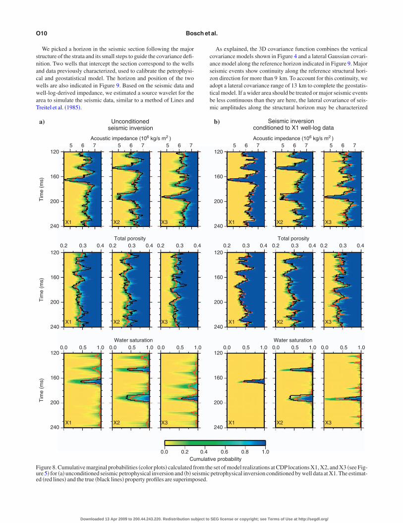
onditioning� at three different distances from the well, correspond-ng to locations X1, X2, and X3 in Figure 5. Color plots indicate therobability of the property’s true value being smaller than or equal tohe property axis value, fully describing the uncertainty of the prop-rty profiles inferred with the inversion. In our color scale, greenlus clear blue areas approximately demark a 0.9 uncertainty bar.he figure also shows the true and estimated property profiles foromparison. Figure 8b is the corresponding probability plots for theetrophysical seismic inversion conditioned to the well-log data atosition X1. Comparing this case with the unconditioned inversion,e can verify �1� smaller uncertainties, �2� uncertainties reducingith the distance to the conditioning well log, and �3� higher fre-uency content in the estimated profiles.

INVERSION RESULTS FOR A GAS RESERVOIR

We apply the inversion method to a stacked and time-migratedmall-incidence-angle �within 18° from the vertical� seismic data setn an area of a producing gas reservoir; a section of the seismic data ishown in Figure 9. The area for the inversion corresponds to a clasticequence with good lateral continuity affected by small faults andild deformation. As indicated, there is no oil presence in the area;

hus, the possible fluids are brine and gas.

g)

h)

i)

estimated using the optimization method: �a-c� cokriging true well-nditioning, and �g-i� joint seismic and well-log-based petrophysicalack dashed line.

ctionsl-log coy the bl


snacwwaT

caszatbm

Fue

O10 Bosch et al.

We picked a horizon in the seismic section following the majortructure of the strata and its small steps to guide the covariance defi-ition. Two wells that intercept the section correspond to the wellsnd data previously characterized, used to calibrate the petrophysi-al and geostatistical model. The horizon and position of the twoells are also indicated in Figure 9. Based on the seismic data andell-log-derived impedance, we estimated a source wavelet for the

rea to simulate the seismic data, similar to a method of Lines andreitel et al. �1985�.

5 6 7 5 6 7 5 6 7

0.2 0.3 0.4 0.2 0.3 0.4 0.2 0.3 0

0.0 0.5 1.0 0.0 0.5 1.0 0.0 0.5

0.0 0.2

120

160

200

240

120

160

200

240

120

160

200

240

Tim

e(m

s)Tim

e(m

s)Tim

e(m

s)

Acoustic impedance (106 kg/s m2 )

Total porosity

Water saturation

Cu

Unconditionedseismic inversion

a)

X1 X2 X3

X1 X2 X3

X1 X2 X3

igure 8. Cumulative marginal probabilities �color plots� calculated fre 5� for �a� unconditioned seismic petrophysical inversion and �b� sd �red lines� and the true �black lines� property profiles are superimp


As explained, the 3D covariance function combines the verticalovariance models shown in Figure 4 and a lateral Gaussian covari-nce model along the reference horizon indicated in Figure 9. Majoreismic events show continuity along the reference structural hori-on direction for more than 9 km. To account for this continuity, wedopt a lateral covariance range of 13 km to complete the geostatis-ical model. If a wider area should be treated or major seismic eventse less continuous than they are here, the lateral covariance of seis-ic amplitudes along the structural horizon may be characterized

5 6 7 5 6 7 5 6 7

0.2 0.3 0.4 0.2 0.3 0.4 0.2 0.3 0.4

0.0 0.5 1.0 0.0 0.5 1.0 0.0 0.5 1.0

0.6 0.8 1.0

120

160

200

240

120

160

200

240

120

160

200

240


Total porosity

Water saturation

ve probability

Seismic inversionconditioned to X1 well-log data

b)

X1 X2 X3

X1 X2 X3

X1 X2 X3

e set of model realizations at CDPlocations X1, X2, and X3 �see Fig-petrophysical inversion conditioned by well data at X1. The estimat-

.4

1.0

0.4mulati

rom theismicosed.


ar

tgdcstsb

i�stcppd1

R

sc1r�lWacbw

tdPtgsntatm

wtiameTapct

iiAaTlu

�btesaarbtbir

R

umstrveszqp

pFwbpb

Foadlu


nd modeled for constructing the horizontal component of the cova-iance function, as done for the vertical components in Figure 4.

We present the results of the estimated property fields followinghe same three procedures categorized for the synthetic tests: �1�eostatistical estimation, �2� petrophysical seismic inversion uncon-itioned to well-log data, and �3� petrophysical seismic inversiononditioned to well-log data. In these categories, we apply the twoolution methods: Monte Carlo sampling and optimization. Parame-ers defining the petrophysical and geostatistical models are theame for the two solution methods and correspond to the model cali-ration described previously.

Figure 6c and d shows the progress of seismic data residuals withterations measured in 2 statistic for the CDP model at location X1Figure 9�. Iterations for the Monte Carlo method �Figure 6c� corre-pond to steps in the Markov chain associated with perturbations ofhe model configurations. Estimated fields and probabilities are cal-ulated from the set of realizations generated during the samplinghase of the chain. A similar plot is shown for the optimization ap-roach �Figure 6d�, with each iteration corresponding to a model up-ate after constructing and solving the linear system of equations0–12.

esults with the optimization solution

Property sections obtained with the optimization solution arehown in Figure 10 and correspond to optimal values: maximumombined probability density values obtained by solving equations0–12 after several iterations, as shown in Figure 6d. The column ar-angement of the plots corresponds to the geostatistical solutioncokriging�, the seismic inversion with no conditioning to the well-og W1 data, and the seismic inversion conditioned to the well-log

1 data. For all of the plots, the corresponding well-log propertiesre superimposed at well-path locations of wells W1 and W2 foromparison with the properties estimated with the inversion. Num-ers at the bottom of the sections indicate the correlation between theell log and the inversion-estimated properties for each case.In Figure 10a-c, the geostatistical estimate shows the extrapola-

ion of the conditioning well logs at position W1 along the structuralirection; the three properties match the well log at the intersection.roperties progressively tend to the prior mean with increasing dis-

ance from the conditioning well log, e.g., the water saturation at theas reservoir progressively reduces away from well W1. Compari-on with the well W2 well-log data shows that major features conve-iently have been extrapolated in space because the structure is par-icularly continuous. However, the geostatistical estimation does notccount for the location of medium heterogeneities and the magni-ude of property contrasts imprinted on the seismic amplitude infor-

ation.For the seismic petrophysical inversion �Figure 10d-f�, there is no

ell constraint; wells are superimposed on the section at their loca-ions W1 and W2 only for comparison with the inversion results. Themage shows that the estimated impedance and water saturation havegood match with the corresponding well logs for thick strata, com-ensurate with the frequency content of the seismic data, as expect-

d; corresponding correlations are shown at the bottom of the plots.he gas saturation looks continuous between the two wells, and nodditional gas strata are present, which coincides with independentroduction information. On the other hand, the low impedance asso-iated with the gas-bearing sand reservoir is mapped partially intohe porosity field and water saturation. This results from the common


nfluence of the two reservoir properties on the acoustic impedance,n this case overestimating the porosity at the site of the reservoir.lso, high well-log porosities that correspond to a shale seal located

t approximately 10 ms above the gas reservoir are underestimated.he correlation of the estimated porosity and the well-log porosity is

ower than correlations obtained for the other two properties for thenconditional seismic inversion.

The seismic inversion conditioned with the W1 well-log dataFigure 10g-i� improves the match of the estimated properties withoth wells �conditioning W1 and blind test W2�. Improved correla-ions are shown at the bottom of the figures for all three model prop-rties — acoustic impedance, water saturation, and total porosity —howing that the well-log information contributes to the resolutioncross saturation and porosity, which have coupled effects on thecoustic impedance.Also, the plots reveal the increase in the verticalesolution for all estimated property fields where thinner strata haveeen inferred. The inferred sections are not a plain extrapolation ofhe W1 well-log data, as in the case of the geostatistical estimation,ecause they include the medium lateral heterogeneities imprintedn the seismic data. The gas saturation shows continuity along theeservoir.

esults with the Monte Carlo solution

The many realizations produced with the sampling algorithm aresed to calculate the estimated fields and probabilities for the threeodel properties. Figure 8c shows the progress of seismic data re-

iduals and the length of the sampling chain for the real-case applica-ion. We used 35,000 iterations of the Monte Carlo sampling algo-ithm per trace with a burn-in phase of 2000 interations, which pro-ided 33,000 realizations in the sampling phase of the process. Thestimated property fields obtained with the Monte Carlo method areimilar to the sections shown in Figure 10 estimated with the optimi-ation approach. In addition, by constructing the cumulative fre-uency of the realizations, we estimated the marginal cumulativerobability distribution for each property.

Figure 11a shows the cumulative probability plots for the seismicetrophysical inversion with no well constraints for three CDPs inigure 9, giving a complete description of the uncertainty associatedith the estimate. The color plotted at each point indicates the proba-ility that the property axis value is greater than or equal to the trueroperty value for the corresponding time. Intermediate plot tonesetween yellow and dark blue can be regarded as marking uncertain-

igure 9. Seismic section that corresponds to a time-migrated stackf small incidence angles �18° from the vertical�. Superimposedre the structural horizon used to guide lateral covariances �dot-ashed black line�, wells W1 and W2 �dashed line�, and an additionalocation X1 �also dashed white line� used for probability plots in Fig-re 11.


tcseicltCplm

rloawcsa

t

lfiidnafsput

terpspmw

a

b

c

Ftdd

O12 Bosch et al.

y bars around the estimated value of the property; the plot zone en-ompassing the green and clear blue areas approximately corre-ponds to a 0.9 probability error bar. We superimpose the prior prop-rty field, which is a linear trend adjusted to the well-log data, and thenversion-estimated field to the probability plot. Two of the locationsorrespond to well sites; for comparison, we superimpose the well-og-derived property sampled at 1-ms intervals. Correlations be-ween the well-log and inversion estimates obtained with the Montearlo method are shown at the bottom of the plots. Note the appro-riate location and magnitude of the water-saturation prediction re-ated to the gas reservoir and the lower frequency content of the seis-

ic inversion result, compared with the well log sampled at 1 ms.Figure 11b shows the same probability plots corresponding to the

esults of the seismic petrophysical inversion constrained with well-og data corresponding to well W1. The estimated result and the pri-r profiles, which in this case correspond to the cokriging estimate,re superimposed; at the conditioning well W1 and the blind testell W2, the well-log-derived properties are also superimposed. We

an see from these probability plots that the uncertainty is muchmaller at site W1 and increases progressively for sites X1 and W2,s expected.

A few other features are worth mentioning. First, near the condi-ioning well, the estimated properties closely approximate the well-

Acoustic Impedance Acoust

Total porosity

Underestimatedporosities Overe

sand

Unsha

Overestimatedwater saturation

Water saturation

)

0.48

0.36

0.91

0.45

0.84

0.43

0.99

0.99

0.99

Wa

Tim

e(m

s)

Distance (m)

2360

2400

2440

2480

2520

2560

2600

0 3000 6000 9000 0 3000

2360

2400

2440

2480

2520

2560

2600

0 3000

2360

2400

2440

2480

2520

2560

2600

0 3000 6000 9000

Geostatistical estimationfrom well data

Uncondiseismic in

W1 DistanceW2W1 W2 W1d)

) e)

) f)

Tim

e(m

s)T

ime

(ms)

igure 10. Matrix of plots corresponding to results of the optimizationion. �a-c� Cokriging of well data along the structural horizon. �d-f� Sitioning. �g-i� Sections estimated by the seismic petrophysical inveerived properties are superimposed on the corresponding inversion


og data. Second, our model allows for deviations of the estimatedeld from the well-log data attributable to the nugget terms modeled

n the covariance functions, which implies an amount of indepen-ence between the well data and the property field estimated at theearest CDP. Third, locations and magnitudes of water saturation aredequate at blind test well W2. Fourth, porosity prediction improvesrom the one corresponding to the unconditioned seismic inversionhown in Figure 11a. Fifth, the vertical resolution of the estimatedroperties improves.Also, the location and magnitude of the gas sat-ration at the reservoir level adequately match the well W2 satura-ion derived from the well-log data.

DISCUSSION

We would like to highlight different assumptions and simplifica-ions made when implementing the method. The petrophysical mod-l is not general purpose and has been developed specifically for gaseservoirs without oil. Different petrophysical models could be im-lemented, depending on the reservoir situation. Gassmann fluidubstitution relations, for instance, could improve the modeling ofartial saturation effects on acoustic impedance. A review of com-on predictive relationships between porosity and compresional-ave velocity, and their combination with Wood’s emulsion equa-

dance

dy

Resolvedshale seal

rosity

0.61

0.40

0.89

0.89

0.86

0.99

0.62

0.57

0.94

Total porosity

ration Water saturation

Wat

ersa

tura

tion

0.25

0.30

0.35

0.40

Aco

ustic

impe

danc

e

(10

kg/s

m2 )

6

5

6

7

8

Tota

l por

osity

0.0

0.2

0.4

0.6

0.8

1.0

Acoustic Impedance

9000

2360

2400

2440

2480

2520

2560

2600

9000

2360

2400

2440

2480

2520

2560

2600

0 3000 6000 9000

2360

2400

2440

2480

2520

2560

2600

0 3000 6000 9000

Seismic inversionconditioned to well W1 data

Distance (m)W2 W1 W2g)

h)

i)

ion method for acoustic impedance, total porosity, and water satura-estimated by seismic petrophysical inversion with no well-log con-

onditioned to well W1 data. At well paths W1 and W2, the well-log-tes for comparison.

ic Impe

stimateporositi

resolvedle seal

Total po

ter satu

6000

6000

tionedversion

(m)

inversectionsrsion cestima


tccAc

dfmvp

FcXp


ion, is given in Mavko et al. �2003� and Brereton �1992�. With anyhoice of relationships, validation and calibration of the petrophysi-al transform with the actual well-log data from the area are needed.lso, more complete petrophysical models can be enhanced to in-

lude other parameters, such as facies, to improve deterministic pre-

0.0 0.2

2400

2440

2480

2520

2560

5 6 7

0.2 0.3 0.4 0.2 0.3 0.4 0.2 0.3

0.0 0.5 1.0

Time(m

s)

W1

0.46

0.82 0.63

0.62

X1

W1

W1

X1

X1

W2

W2

W2

0.40.50

5 6 7 5 6

0.0 0.5 1.0 0.0 0.5

2400

2440

2480

2520

2560

2400

2440

2480

2520

2560

Time(m

s)Time(m

s)


Unconditionedseismic inversion

a)

Total porosity

Water saturation

Cu

igure 11. Cumulative marginal probabilities for the model propertieonditioned seismic petrophysical inversion and �b� seismic petroph1, and W2 �see Figure 9�. The estimated property profiles �red linesrofiles �black lines� are superimposed.


iction of the elastic parameters. In cases where matrix lithology ef-ects are particularly relevant or fluid-property contrasts are lessarked, as in our case, we suggest extending the application to in-

ert multiple offset �or angle� seismic data to estimate a more com-lete set of reservoir properties.

0.6 0.8 1.0

W1 X1

W1

W1

X1

X1

W2

W2

W2

0.99 0.81

0.83 0.64

0.560.87

0.2 0.3 0.4 0.2 0.3 0.4 0.2 0.3 0.4

5 6 7 5 6 7 5 6 7

0.0 0.5 1.0 0.0 0.5 1.0 0.0 0.5 1.0


Seismic inversionconditioned to X1 well-log data

b)

Total porosity

Water saturation

e probability

r plots� calculated from the set of joint model realizations for �a� un-inversion conditioned to well W1 data shown at CDP locations W1,rior property profile �white lines�, and the well-log-derived property

0.4

0.4

8

7

1.0

mulativ

s �coloysical�, the p


irrofiatptvrp

�khrahIsatf

rctseewttilmspa

psmpvHmmfpmupgmri

si

lsamlptiac9dssr

soMpnmamtscpp

dsvstonawrca

tmmcrmaswtt

O14 Bosch et al.

An important advantage of our general petrophysical formulations that we use a mixed model, combining petrophysical deterministicelationships and random deviations. Well-log statistics may not beepresentative of the reservoir because of limits on the well numbersr because wells are not drilled randomly. Thus, a purely empiricalt of a function to the well-log data is sensible with poor data cover-ge. In our model, we use petrophysical relationships calibrated tohe well-log data for more robust modeling, consistent with commonetrophysical knowledge. On the other hand, none of the determinis-ic petrophysical transforms fully explains the relation between theariables. Thus, describing well-data deviations from the calibratedelationships allows us to account for the variability of mediumroperties from these relations.

Upscaling recipes and relationships are a matter of discussionLindsay and Van Koughnet, 2001; Liner and Fei, 2007�. Well-nown situations correspond to the two extremes in wavelength andeterogeneity-size ratios, given by the effective media and ray theo-ies. However, behavior in many common cases is more complicatednd involves a combination of the two phenomena. In real cases, weave a distribution of wavelength and medium heterogeneity sizes.n intermediate cases, dispersion and apparent attenuation can be ob-erved, and different approaches have been proposed �Chapman etl., 2006�. In our case, the dominant period is approximately 20imes larger than the high-resolution model layer thickness; there-ore, rescaling to a seismic resolution layering is required.

We rescale between our low and high model resolution scales di-ectly in the impedance. This is convenient in our formulation be-ause impedance is the elastic parameter in our model, whereas be-ween the original well-log sampling and the high-resolution modelcale, we use common effective media expressions. Our upscalingxpression for impedance combines ray and effective media consid-rations and produces results within the two bounds. For the scalese relate in our synthetic and real implementations, our tests with

he actual data of the area show that differences are negligible be-ween the effective media average, the ray theory average, and ourntermediate model average of the impedance. However, we formu-ate this issue for generality of the method because it relates the seis-

ic and subseismic scales. In different conditions of model-timeampling, source-frequency composition, or variability of mediumroperties, the difference in the smoothing approach used for thecoustic impedance could be significant.

Because effects of total porosity and gas saturation in acoustic im-edance are coupled, their estimation could be unresolved from theole information rendered by the near-vertical incidence-angle seis-ic data. The additional information provided by the nonlinear

etrophysical model and the geostatistical characterization of reser-oir properties contribute to the resolution of the two properties.owever, as shown in the synthetic tests for the unconditioned seis-ic petrophysical inversion, some features of high gas saturation areapped partially as high porosities, and vice versa. The coupled ef-

ect is given at the level of the petrophysical model because the tworoperties are uncorrelated at the level of the prior statistical infor-ation. Conditioning the inversion to well-log data largely contrib-

tes to resolving the ambiguity resulting from the petrophysical cou-led effect of the two reservoir properties. On the other hand, plaineostastistical estimation �cokriging� based on the well-log dataisses information between the wells carried by the seismic data and

elated with strata heterogeneities and structural features of majornterest in reservoir description. The combination of well-log and


eismic inversion builds on the corresponding assets of each type ofnformation to estimate the property fields better.

Another issue of reservoir characterization is the possibility of de-ineating thin strata. Because of the lateral covariance in the geo-tatistical model, the high-resolution well-log data extrapolationlong the structural directions contributes to the property-field esti-ates. Joint seismic and well-log inversion improves vertical reso-

ution as a result of the contribution of the well-log data. This is notarticularly important for the gas-bearing sand, which has a layerhickness commensurate with the seismic dominant wavelength, butt is clear for other thinner strata. In particular, the acoustic imped-nce and the porosity sections resolve thin stratification that matchesorresponding thin strata at the blind test well W2, located more thankm from the conditioning well W1. Correlation is larger and rms

eviation is smaller for the joint seismic and well-log-based inver-ion than for each of the disjoint components for geostatistical andeismic information. Similar results on improving the joint verticalesolution are shown in the synthetic tests.

Because they are based on the same general formulation and as-umptions, the results obtained from the Monte Carlo sampling andptimization methods are similar in the method’s major features.inor differences result from particularities of the two-solution ap-

roach. Concerning execution times, it is important to notice that theumber of iterations shown in Figure 6 for the Monte Carlo and opti-ization methods cannot be used straightforwardly to compare the

ssociated computation effort. A single iteration of the Monte Carloethod is a very fast process, whereas an iteration of the optimiza-

ion method requires solving a large system of equations. For the re-ults shown here, the optimization approach is faster by a factor of 20ompared with the Monte Carlo approach for estimating mediumroperties. However, the Monte Carlo method describes propertyrobabilities �uncertainties� in addition to property estimates.

CONCLUSION

We have developed a general formulation for inverting seismicata under well-log constraints derived from petrophysical and geo-tatistical models. It allows a joint description and inference of reser-oir- and elastic-medium properties. The formulation unifies theteps of geophysical and petrophysical data inversion within a quan-itative scheme, accounting for nonlinear relationships, conditioningf estimated property fields to well-log measurements, and combi-ation of uncertainties. We describe solution methods for two majorpproaches, sampling and optimization, and illustrate the techniquesith a synthetic example and an application to field data from a gas

eservoir. In this specific setting, we invert seismic near-vertical in-idence-angle and well-log data to estimate gas saturation, porosity,nd acoustic impedance jointly.

Results of the numerical tests are coherent with the hypotheses ofhe method. They show that geostatistical interpolation commonly

isses laterally discontinuous features, whereas petrophysical seis-ic inversion �without well conditioning� is limited in frequency ac-

ording to the seismic signal. Also, the latter is limited in resolvingeservoir properties �porosities and saturations�, which can be cross-apped partially for some events because of their coupled effect on

coustic impedance. These issues are improved in the petrophysicaleismic inversion conditioned with well-log data. In the field case,e base our inference parameters on calibrating the petrophysical

ransform and the geostatistical characterization of the well logs andransform deviations.


jueptttt

0cfts

B

B

B

—

B

B

B

C

C

C

D

D

E

G

G

G

G

H

H

HI

L

L

L

L

M

M

M

M

R

S

S

S

S

S

S

T

T

WW


Results of acoustic impedance, water saturation, and porosityointly honor the seismic data, well logs, and petrophysical modelsed for the area. We successfully resolve the property fields delin-ating gas saturation at the level of the reservoir. The seismic petro-hysical inversion constrained by well-log data combines assets ofhe two types of information: increased vertical resolution close tohe well, estimated fields that conform to the well logs at intersec-ions, no smoothing of lateral resolution, and adequate joint resolu-ion of water saturation and porosity.

ACKNOWLEDGMENTS

The authors thank CDCH-Universidad Central of Venezuela �PG-8-00-5631-04/08�, Petrobras Energía Venezuela, and ENI for theirontributions to this research.Also, thanks to the referees and editorsor their reviews and comments. This work was done at the Labora-ory of Geophysical Simulation and Inversion �LSIG� of the Univer-idad Central of Venezuela.

REFERENCES

achrach, R., 2006, Joint estimation of porosity and saturation using stochas-tic rock-physics modeling: Geophysics, 71, no. 5, O53–O63.

ackus, G. E., 1962, Long-wave elastic anisotropy produced by horizontallayering: Journal of Geophysical Research, 67, 4427–4440.

osch, M., 1999, Lithologic tomography: From plural geophysical data to li-thology estimation: Journal of Geophysical Research, 104, 749–766.—–, 2004, The optimization approach to lithological tomography: Com-bining seismic data and petrophysical information for porosity prediction:Geophysics, 69, 1272–1282.

osch, M., L. Cara, J. Rodrigues, A. Navarro, and M. Díaz, 2007, A MonteCarlo approach to the joint estimation of reservoir and elastic parametersfrom seismic amplitudes: Geophysics, 72, no. 6, O29–O39.

rereton, N. R., 1992, Physical property relationships from sites 756 and766: Proceedings of the Ocean Drilling Program, Scientific Results, 123,453–468.

uland, A., and H. Omre, 2003, Bayesian linearized AVO inversion: Geo-physics, 68, 185–198.

hapman, M., E. Liu, and X.-Y. Li, 2006, The influence of fluid-sensitive dis-persion and attenuation on AVO analysis: Geophysical Journal Interna-tional, 167, 89–105.

hiles, J.-P., and P. Delfiner, 1999, Geostatistics: Modeling spatial uncertain-ty: John Wiley & Sons, Inc.

ontreras, A., C. Torres-Verdin, W. Chesters, and K. Kvien, 2005, Joint sto-chastic inversion of petrophysical logs and 3D pre-stack seismic data to as-sess the spatial continuity of fluid units away from wells: Application to aGulf of Mexico deepwater hydrocarbon reservoir: Transactions of the 46thAnnual Logging Symposium, Society of Petrophysicists and Well LogAn-alysts, Paper UUU.

oyen, P. M, 1988, Porosity from seismic data: A geostatistical approach:Geophysics, 53, 1263–1275.

ubrule, O., 2003, Geostatistics for seismic data integration in earth models:SEG.

idsvik, J., P. Avseth, H. More, T. Mukerji, and G. Mavko, 2004, Stochastic


reservoir characterization using prestack seismic data: Geophysics, 69,978–993.

eyer, C. J., 1992, Practical Markov chain Monte Carlo: Statistical Science,7, 473–551.

onzalez, E. F., T. Mukerji, and G. Mavko, 2008, Seismic inversion combin-ing rock physics and multiple-point geostatistics: Geophysics, 73, no. 1,R11–R21.

rechka, V., 2003, Effective media: A forward modeling view: Geophysics,68, 2055–2062.

unning, J., and M. E. Glinsky, 2007, Detection of reservoir quality usingBayesian seismic inversion: Geophysics, 72, no. 3, R37–R49.

aas, A., and O. Dubrule, 1994, Geostatistical inversion—A sequentialmethod of stochastic reservoir modeling constrained by seismic data: FirstBreak, 12, 561–569.

astings, W. K., 1970, Monte Carlo sampling method using Markov chainsand their applications: Biometrika, 57, 97–109.

ilterman, F. J., 2001, Seismic amplitude interpretation: SEG.saaks, E., and R. Srivastava, 1989, An introduction to applied geostatistics:

Oxford University Press.arsen, A. L., M. Ulvmoen, H. Omre, and A. Buland, 2006, Bayesian litholo-gy/fluid prediction and simulation on the basis of a Markov-chain priormodel: Geophysics, 71, no. 5, R69–R78.

indsay, R., and R. Van Koughnet, 2001, Sequential Backus averaging: Up-scaling well logs to seismic wavelengths: The Leading Edge, 20, 188–191.

iner, C., and T. Fei, 2007, The Backus number: The Leading Edge, 26, 420–426.

ines, L., and S. Treitel, 1985, Wavelets, well logs and Wiener filters: FirstBreak, 3, 9–14.avko, G., T. Mukerji, and J. Dvorkin, 2003, The rock physics handbook:Cambridge University Press.osegaard, K., and A. Tarantola, 1995, Monte Carlo sampling of solutions toinverse problems: Journal of Geophysical Research, 100, 12431–12447.ukerji, T., A. Jørstad, P. Avseth, G. Mavko, and J. R. Granli, 2001, Mappinglithofacies and pore-fluid probabilities in a North Sea reservoir: Seismicinversions and statistical rock physics: Geophysics, 66, 988–1001.ukerji, T., G. Mavko, D. Mujica, and N. Lucet, 1995, Scale-dependent seis-mic velocity in heterogeneous media: Geophysics, 60, 1222–1233.

io, P., T. Mukerji, G. Mavko, and D. Marion, 1996, Velocity dispersion andupscaling in a laboratory-simulated VSP: Geophysics, 61, 584–593.

altzer, R., C. Finn, and O. Burtz, 2005, Predicting Vshale and porosity usingcascaded seismic and rock physics inversion: The Leading Edge, 24, 732–736.

choenberg, M., and F. Muir, 1989, A calculus for finely layered anisotropicmedia: Geophysics, 54, 581–589.

engupta, M., and R. Bachrach, 2007, Uncertainty in seismic-based pay vol-ume estimation: Analysis using rock physics and Bayesian statistics: TheLeading Edge, 24, 184–189.

mith, A. F., and G. O. Roberts, 1993, Bayesian computations via the Gibbssampler and related Markov chain Monte Carlo methods: Journal of theRoyal Statistical Society, 55, 3–23.

pikes, K., T. Mukerji, J. Dvorkin, and G. Mavko, 2007, Probabilistic seis-mic inversion based on rock-physics models: Geophysics, 72, no. 5, R87–R97.

tovas, A., and B. Arntsen, 2006, Vertical propagation of low-frequencywaves in finely layered media: Geophysics, 71, no. 3, T87–T94.

ierney, L., 1994, Markov-chains for exploring posterior distributions: An-nals of Statistics, 22, 1702–1762.

orres-Verdin, C., M. Victoria, G. Merletti, and J. Pendrel, 1999, Trace-basedand geostatistical inversion of 3-D seismic data for thin-sand delineation:An application in San Jorge Basin, Argentina: The Leading Edge, 19,1070–1077.ood, A. W., 1955,Atextbook on sound: Macmillan Publ. Co..yllie, M. R. J., A. R. Gregory, and L. W. Gardner, 1956, Elastic wave veloc-ities in heterogeneous and porous media: Geophysics, 21, 41–70.


Documents

Petrophysical seismic inversion conditioned to well-log ...Petrophysical seismic inversion conditioned to well-log data: Methods and application to a gas reservoir Miguel Bosch1, Carla