Embed Size (px)
Citation preview

Petri Nets – Lecture 1
Chen ChenSep. 28th, 2011
2011/9/28 \course\867-11F\Topic-2.ppt 1

Outline
• History of Petri Nets• Basic Terminologies• Comparing with FSM• Petri Net Properties
2011/9/28 \course\867-11F\Topic-2.ppt 2
Invention of Petri Nets
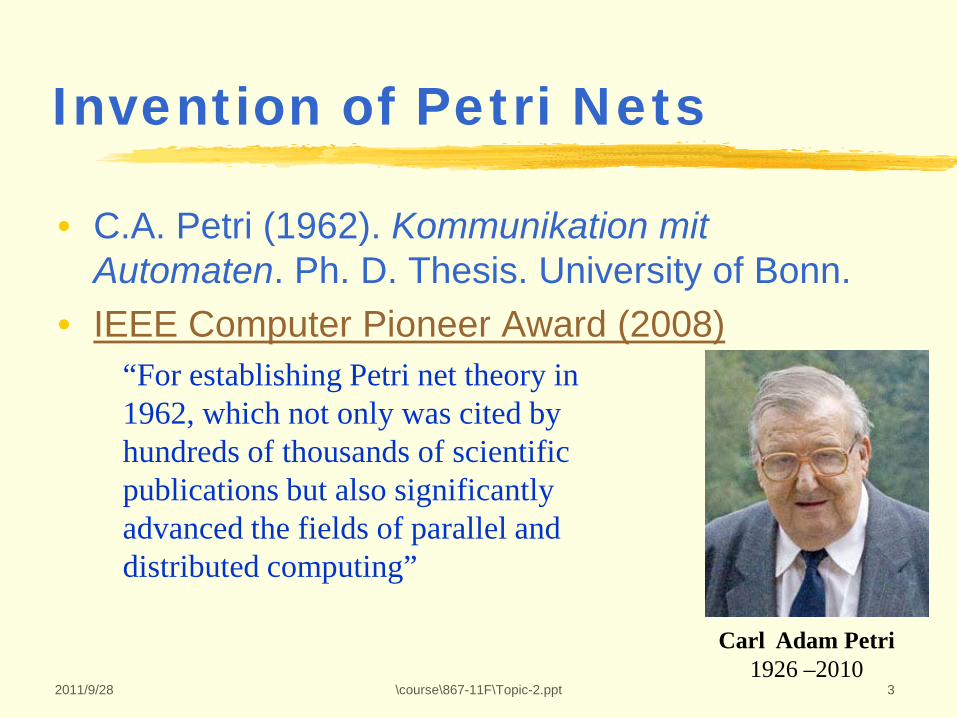
• C.A. Petri (1962). Kommunikation mitAutomaten. Ph. D. Thesis. University of Bonn.
• IEEE Computer Pioneer Award (2008)
2011/9/28 \course\867-11F\Topic-2.ppt 3
Carl Adam Petri1926 –2010
“For establishing Petri net theory in 1962, which not only was cited by hundreds of thousands of scientific publications but also significantly advanced the fields of parallel and distributed computing”

Introduction to Petri Nets Theory
• A theory of systems for modeling concurrency and synchronization
• Feature Graphical representation Simplicity Expressiveness for concurrency and
asynchronous operations
2011/9/28 \course\867-11F\Topic-2.ppt 4

ISO/IEC 15909 (2011)Petri Nets Standard
Rudiger Valk (1998)Elementary Object Nets
M.K. Molly (1982)Stochastic Petri Nets
Chiola, Dutheillet, Franceschinis, S. Haddad. (1991)
Well-Formed Coloured Nets
History of Petri Nets
2011/9/28 \course\867-11F\Topic-2.ppt 5
1960 1970 1980 1990 2000 2010C.A. Petri (1962)
Invention of Petri Nets
Holt and Commoner (1970)Graphical expression of PN
Marked Graph
Ramchandani (1973)Timed Petri Nets
Kurt Jensen (1981)Colored Petri Nets
E. P. Dawis, J. F. Dawis, Wei-Pin Koo(2001)Dualistic Petri Nets
Bail, Alla, David (1991)Hybrid Petri Nets
R. David & H. Alla (1987)Continuous Petri Nets
Hack (1972)Free-choice Petri Nets
Simple Petri Nets
Buchs and Guelfi (1991)Object Oriented Petri Net
Haddad & Poitrenaud (2007)Recursive Petri Nets
First PN
Sub-class of PN
Extension of PN
Normalization of PN

Outline
• History• Basic Terminologies• Comparing with FSM• Petri Net Properties
2011/9/28 \course\867-11F\Topic-2.ppt 6

Example: Critical Section
• 3 users try to access the same CS• Only one user can access CS each time
2011/9/28 \course\867-11F\Topic-2.ppt 7
Critical Section
3 tokens = 3 users 1 token = lock place
transition
token
t2
p2
p3
p1
t1
arc

Example: Critical Section
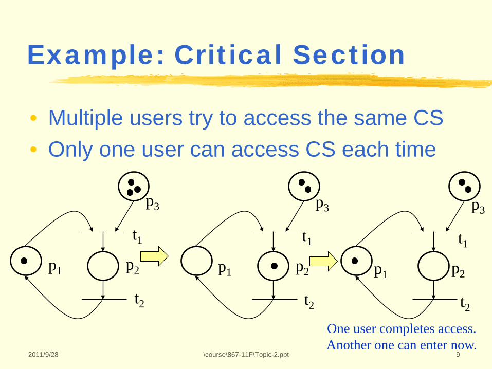
• Multiple users try to access the same CS• Only one user can access CS each time
2011/9/28 \course\867-11F\Topic-2.ppt 8
One user entered CSThe others have to wait
t2
p2
p3
p1
t1
t2
p2
p3
p1
t1
Example: Critical Section
• Multiple users try to access the same CS• Only one user can access CS each time
2011/9/28 \course\867-11F\Topic-2.ppt 9
One user completes access.Another one can enter now.
t2
p2
p3
p1
t1
t2
p2
p3
p1
t1
t2
p2
p3
p1
t1

Example: Producer-Consumer
2011/9/28 \course\867-11F\Topic-2.ppt 10
Producer
Consumer A Consumer B
Task Buffer
Producer produces tasks and put the tasks in the task buffer.Consumers take tasks from the task buffer and execute them.One task can only be executed by one consumer – either A or B.
1 2 3

Example: Producer-Consumer
2011/9/28 \course\867-11F\Topic-2.ppt 11
Producer
Consumer A Consumer B
Task Buffer
1 2 3
Producer produced one task.Either A or B can be fired. But only one will be fired!

Example: Producer-Consumer
2011/9/28 \course\867-11F\Topic-2.ppt 12
Producer
Consumer A Consumer B
Task Buffer
1 2 3
After firing A or B, the task is executed.

Example: Producer-Consumer
2011/9/28 \course\867-11F\Topic-2.ppt 13
Producer
Consumer A Consumer B
Task Buffer
What’s the difference between Petri Nets and Dataflow?
Petri NetsDataflow (similar structure
but different semantics)
What will happen after token pushing?

Definition of a Petri Net (Self-reading)
• A Petri Net is a bipartite graph (P,T,A) that comprises of A set of transitions: T A set of places: P A set of directed arcs: A
2011/9/28 \course\867-11F\Topic-2.ppt 14
a transition a place

Firing Rules (Self-reading)
•
2011/9/28 \course\867-11F\Topic-2.ppt 15

Petri Net Marking (Self-reading)
•
2011/9/28 \course\867-11F\Topic-2.ppt 16

Outline
• History• Basic Terminologies• Comparing with FSM• Petri Net Properties
2011/9/28 \course\867-11F\Topic-2.ppt 17
Example: Two’s Complement
• What is two’s complement?• How to compute two's complement?
2011/9/28 \course\867-11F\Topic-2.ppt 18

Example: Two's Complement (cont.)
• What is two's complement?• How to compute two's complement? flip all bits, and then plus a carry bit Assume B = 110, then -B = 001 + 1 = 010
2011/9/28 \course\867-11F\Topic-2.ppt 19

Example: Two's Complement (cont.)
• What is two's complement?• How to compute two's complement? flip all bits, and then plus a carry bit Assume B = 110, then -B = 001 + 1 = 010 Compute two's complement of 110 from low bit flip(0) + carry bit 1 + 1 = 0 & carry bit flip(1) + carry bit 0 + 1 = 1 flip(1) 0
2011/9/28 \course\867-11F\Topic-2.ppt 20

Example: Two's Complement (cont.)
2011/9/28 \course\867-11F\Topic-2.ppt 21
q1 q2
1/1
R/R
0/0
R/R
0/1
1/0State q1: need to add carry bitflip(0) + carry bit 1 + 1 = 0 + carry bitflip(1) + carry bit 0 + 1 = 1
State q2: no need to add carry bitflip(0) 1 flip(1) 0
R means reset of computation

Example: FSM (cont.)
2011/9/28 \course\867-11F\Topic-2.ppt 22
q1 q2
1/1
R/R
0/0
R/R
0/1
1/0
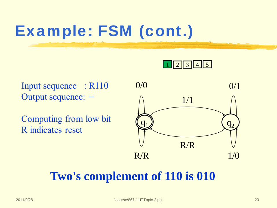
Now try to compute two's complement of 110
Example: FSM (cont.)
2011/9/28 \course\867-11F\Topic-2.ppt 23
q1 q2
1/1
R/R
0/0
R/R
0/1
1/0
1 2 3 4 5
Two's complement of 110 is 010

Example: FSM (cont.)
2011/9/28 \course\867-11F\Topic-2.ppt 24
q1 q2
1/1
R/R
0/0
R/R
0/1
1/0
1 2
Input sequence : R11Output sequence: 0
Computing from low bitR indicates reset
3 4 5
Two's complement of 110 is 010

Example: FSM (cont.)
2011/9/28 \course\867-11F\Topic-2.ppt 25
q1 q2
1/1
R/R
0/0
R/R
0/1
1/0
1 2
Input sequence : R1Output sequence: 10
Computing from low bitR indicates reset
3 4 5
Two's complement of 110 is 010
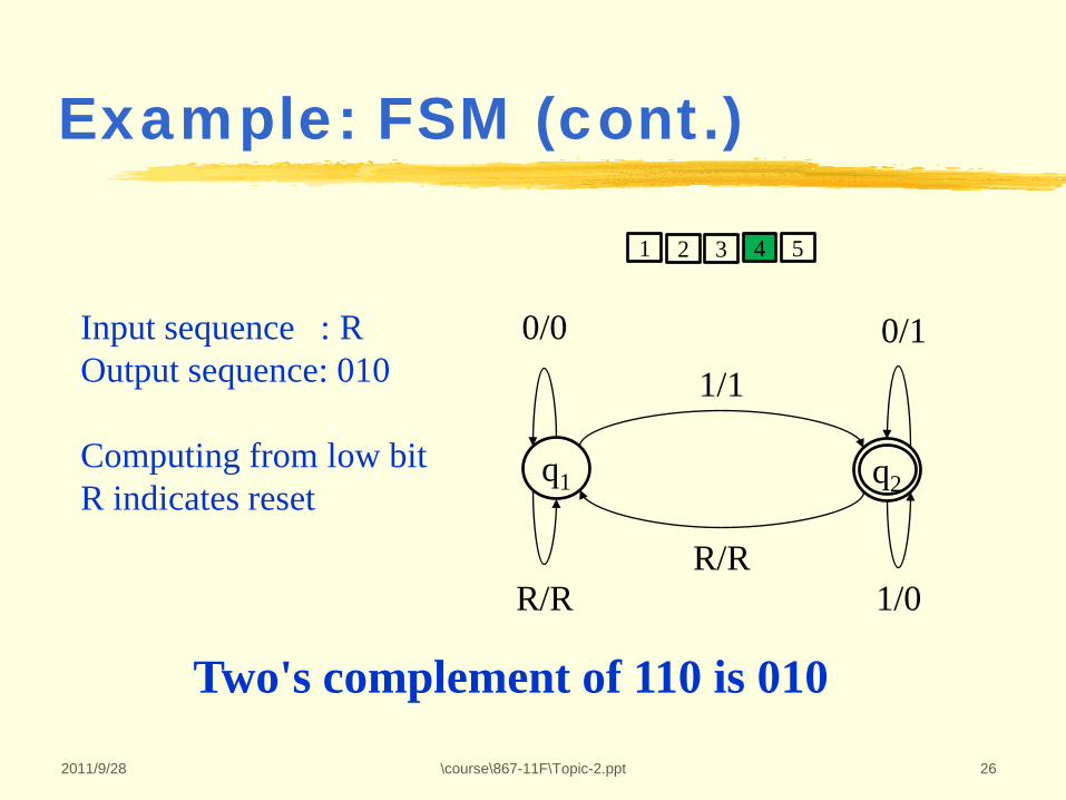
Example: FSM (cont.)
2011/9/28 \course\867-11F\Topic-2.ppt 26
q1 q2
1/1
R/R
0/0
R/R
0/1
1/0
1 2
Input sequence : ROutput sequence: 010
Computing from low bitR indicates reset
3 4 5
Two's complement of 110 is 010

Example: FSM (cont.)
2011/9/28 \course\867-11F\Topic-2.ppt 27
q1 q2
1/1
R/R
0/0
R/R
0/1
1/0
1 2 3 4 5
Two's complement of 110 is 010

Finite State Machine (FSM)Self-reading
•
2011/9/28 \course\867-11F\Topic-2.ppt 28

Important Features of FSM
2011/9/28 \course\867-11F\Topic-2.ppt 29
What are the features?

Important Features of FSM
2011/9/28 \course\867-11F\Topic-2.ppt 30
What are the features?
FSM is always at a single active state!
A single input event triggers state transition!

Important Features of FSM
2011/9/28 \course\867-11F\Topic-2.ppt 31
What are the features?
FSM is always at a single active state!How to represent multiple active states
as a single active state?A single input event triggers state transition!
How to represent synchronization between multiple states?

Another Example: 2-Stage Pipeline Modeling
2011/9/28 \course\867-11F\Topic-2.ppt 32
Input sequence Output sequence
Unit1 Unit2
Each unit can be modeled by a three-state FSM
ready for input
ready to outputbusy
Unit I (I = 1,2)
a
b c

Another Example: 2-Stage Pipeline Modeling (cont.)
2011/9/28 \course\867-11F\Topic-2.ppt 33
Input sequence Output sequence
Unit1 Unit2
How to model the two units together in FSM?

Another Example: 2-Stage Pipeline Modeling (cont.)
2011/9/28 \course\867-11F\Topic-2.ppt 34
Input sequence Output sequence
Unit1 Unit2
How to model the two units together in FSM?– cross-functional states
State aa’: Unit1 is ready for input & Unit2 is ready for inputState ba’: Unit1 is busy & Unit2 is ready for inputState ca’: Unit 1 is ready to output & Unit2 is ready for input
…State cc’: Unit 1 is ready to output & Unit 2 is ready to output

Another Example: 2-Stage Pipeline Modeling (cont.)
2011/9/28 \course\867-11F\Topic-2.ppt 35
ab’
aa’ac’
ba’
bb’
bc’
ca’
cc’
cb’The structure of the FSM for 2-stage pipeline modeling. Inputs and outputs are omitted.

Problems of FSM Modeling of the Pipeline
• Number of states grows exponentially with the number of stages
• The identity of the individual stage lost • The structure information is obscured• Concurrency / synchronization information
cannot be represented
2011/9/28 \course\867-11F\Topic-2.ppt 36

Try Again: 2-Stage Pipeline Modeling by PN
2011/9/28 \course\867-11F\Topic-2.ppt 37
Each unit can be modeled by 3 places and 3 transitions
ready for input
ready to outputbusy
Pickup input data
Done with processing
Output result
Input sequence Output sequence
Unit1 Unit2 Unit I (I = 1,2)

Try Again: 2-Stage Pipeline Modeling by PN (cont.)
2011/9/28 \course\867-11F\Topic-2.ppt 38
ready for input
ready to output
busy
Done with processing
Output result
ready for input
ready to output
busy
Pickup input data
Done with processing
Unit1 transfers intermediate result to Unit2
Input sequence Output sequenceUnit1 Unit2
Pipeline
PN
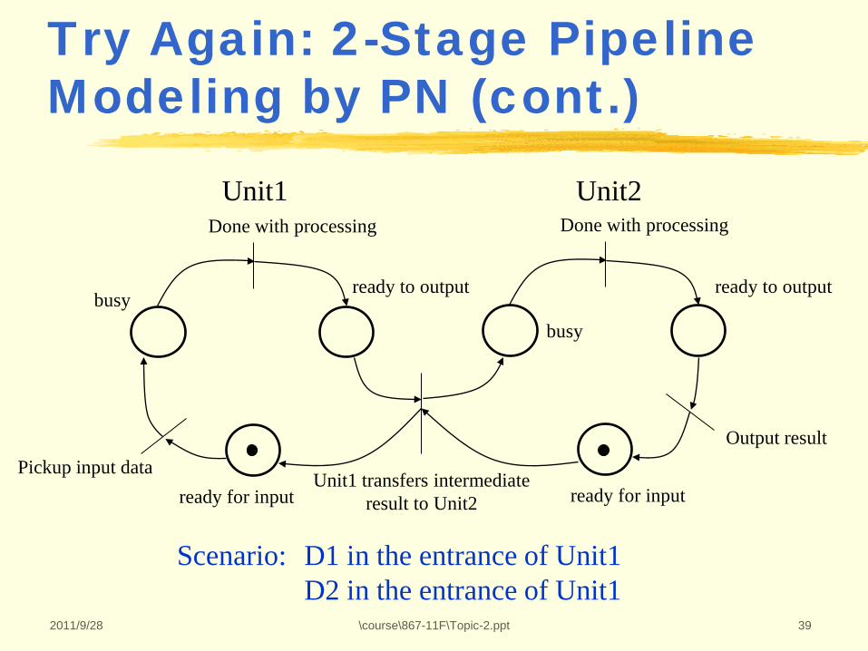
Try Again: 2-Stage Pipeline Modeling by PN (cont.)
2011/9/28 \course\867-11F\Topic-2.ppt 39
ready for input
ready to output
busy
Done with processing
Output result
ready for input
ready to outputbusy
Pickup input data
Done with processing
Scenario: D1 in the entrance of Unit1D2 in the entrance of Unit1
Unit1 Unit2
Unit1 transfers intermediate result to Unit2

Try Again: 2-Stage Pipeline Modeling by PN (cont.)
2011/9/28 \course\867-11F\Topic-2.ppt 40
ready for input
ready to output
busy
Done with processing
Output result
ready for input
ready to outputbusy
Pickup input data
Done with processing
Scenario: D1 being processed by Unit1D2 in the entrance of Unit1
Unit1 Unit2
Unit1 transfers intermediate result to Unit2

Try Again: 2-Stage Pipeline Modeling by PN (cont.)
2011/9/28 \course\867-11F\Topic-2.ppt 41
ready for input
ready to output
busy
Done with processing
Output result
ready for input
ready to outputbusy
Pickup input data
Done with processing
Unit1 Unit2
Scenario: D1 is done by Unit1D2 in the entrance of Unit1
Unit1 transfers intermediate result to Unit2

Try Again: 2-Stage Pipeline Modeling by PN (cont.)
2011/9/28 \course\867-11F\Topic-2.ppt 42
ready for input
ready to output
busy
Done with processing
Output result
ready for input
ready to outputbusy
Pickup input data
Done with processing
Unit1 Unit2
Scenario: D1 being processed by Unit2D2 in the entrance of Unit1
Unit1 transfers intermediate result to Unit2

Try Again: 2-Stage Pipeline Modeling by PN (cont.)
2011/9/28 \course\867-11F\Topic-2.ppt 43
ready for input
ready to output
busy
Done with processing
Output result
ready for input
ready to outputbusy
Pickup input data
Done with processing
Unit1 Unit2
Scenario: D1 is done by Unit2D2 being processed by Unit1
Unit1 transfers intermediate result to Unit2

Try Again: 2-Stage Pipeline Modeling by PN (cont.)
2011/9/28 \course\867-11F\Topic-2.ppt 44
ready for input
ready to output
busy
Done with processing
Output result
ready for input
ready to outputbusy
Pickup input data
Done with processing
Unit1 Unit2
Scenario: Result of D1 is outputted by Unit2D2 is done by Unit1
Unit1 transfers intermediate result to Unit2

Try Again: 2-Stage Pipeline Modeling by PN (cont.)
2011/9/28 \course\867-11F\Topic-2.ppt 45
ready for input
ready to output
busy
Done with processing
Output result
ready for input
ready to outputbusy
Pickup input data
Done with processing
Unit1 Unit2
Scenario: Result of D1 is outputted by Unit2D2 being processed by Unit2
Unit1 transfers intermediate result to Unit2

Try Again: 2-Stage Pipeline Modeling by PN (cont.)
2011/9/28 \course\867-11F\Topic-2.ppt 46
ready for input
ready to output
busy
Done with processing
Output result
ready for input
ready to outputbusy
Pickup input data
Done with processing
Unit1 Unit2
Scenario: Result of D1 is outputted by Unit2D2 is done by Unit2
Unit1 transfers intermediate result to Unit2

Try Again: 2-Stage Pipeline Modeling by PN (cont.)
2011/9/28 \course\867-11F\Topic-2.ppt 47
ready for input
ready to output
busy
Done with processing
Output result
ready for input
ready to outputbusy
Pickup input data
Done with processing
Unit1 Unit2
Unit1 transfers intermediate result to Unit2
Scenario: Result of D1 is outputted by Unit2Result of D2 is outputted by Unit2

Conclusion: Compare PN with FSM
• PN is powerful in constructing composite machines. FSM must do cross product.
• PN is powerful in expressing concurrency. (FSM cannot express concurrency).
• PN is powerful in expressing synchronization.
2011/9/28 \course\867-11F\Topic-2.ppt 48

Outline
• History• Basic Terminologies• Comparing with FSM• Petri Net Properties
2011/9/28 \course\867-11F\Topic-2.ppt 49

Petri Net Properties
• Reachability• Safeness and Boundness• Conservation• Liveness• Persistency• Consistency
2011/9/28 \course\867-11F\Topic-2.ppt 50