Embed Size (px)
Citation preview
Petri Nets
1
Petri nets
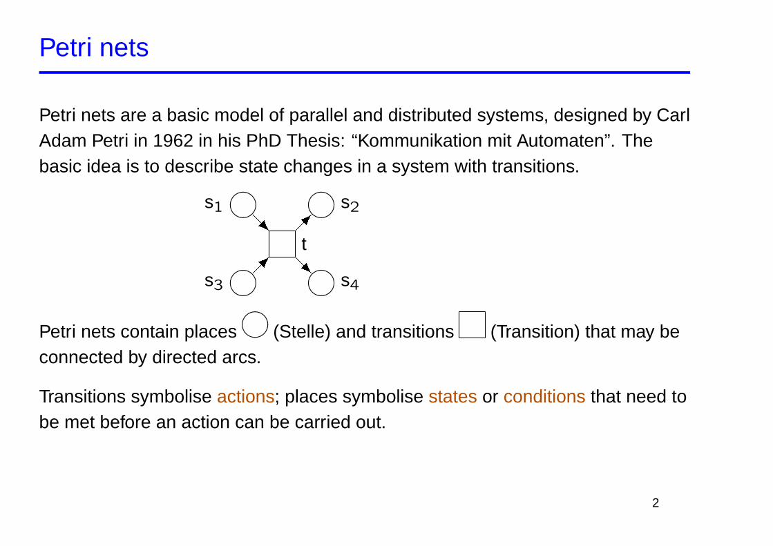
Petri nets are a basic model of parallel and distributed systems, designed by CarlAdam Petri in 1962 in his PhD Thesis: “Kommunikation mit Automaten”. Thebasic idea is to describe state changes in a system with transitions.
����
����
����
����
t���
@@R
@@R
���s1 s2
s3 s4
Petri nets contain places ����
(Stelle) and transitions (Transition) that may beconnected by directed arcs.
Transitions symbolise actions; places symbolise states or conditions that need tobe met before an action can be carried out.
2
Behaviour of Petri nets
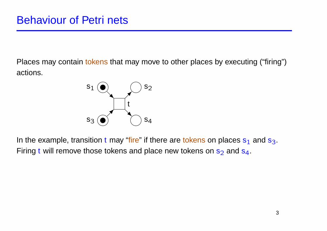
Places may contain tokens that may move to other places by executing (“firing”)actions.
����
����
����
����
t���
@@R
@@R
���s1
}
} s2
s3 s4
In the example, transition t may “fire” if there are tokens on places s1 and s3.Firing t will remove those tokens and place new tokens on s2 and s4.
3
Example: Dining philosophers
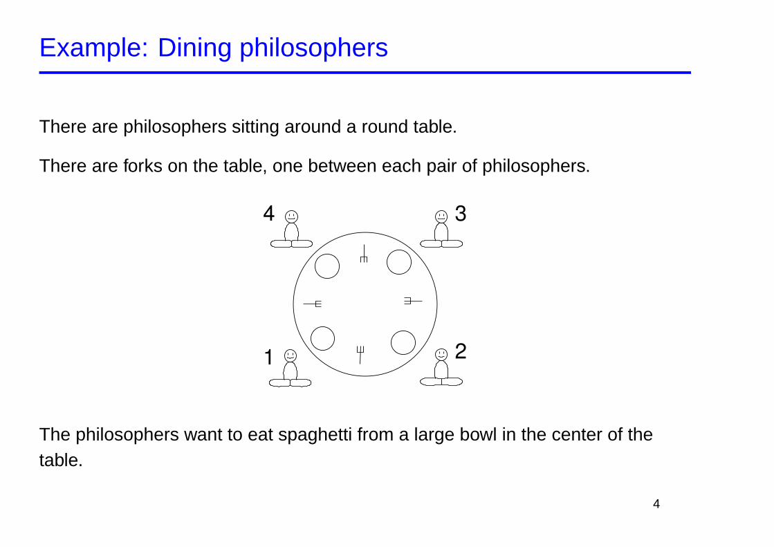
There are philosophers sitting around a round table.
There are forks on the table, one between each pair of philosophers.
4
1 2
3
The philosophers want to eat spaghetti from a large bowl in the center of thetable.
4
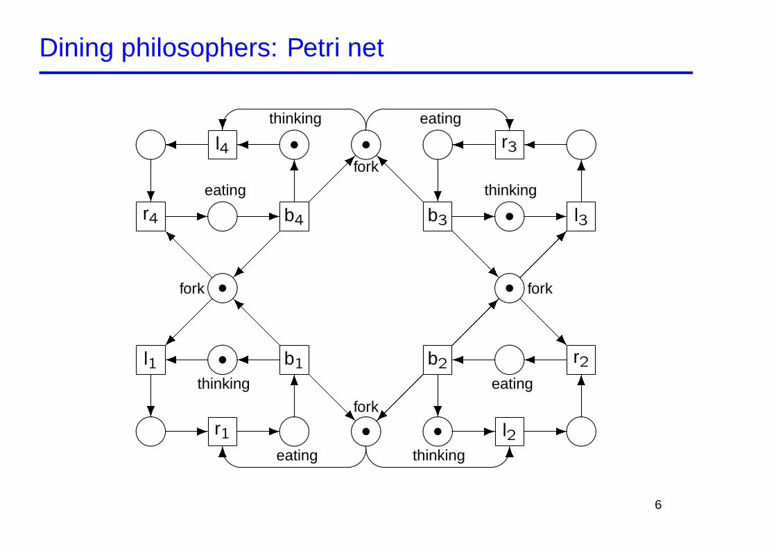
Unfortunately the spaghetti is of a particularly slippery type, and a philosopherneeds both forks in order to eat it.
The philosophers have agreed on the following protocol to obtain the forks:Initially philosophers think about philosophy, when they get hungry they do thefollowing: (1) take the left fork, (2) take the right fork and start eating, (3) returnboth forks simultaneously, and repeat from the beginning
How can we model the behaviour of the philosophers?
5
Dining philosophers: Petri net
����
����
����
����
����
����
����
����
����
����
������������
������������
w
w w
w
w w
w wfork
fork
fork fork
l1 �
��
��
��
?r1- -
& %6
b16
�
@@@@@@R
@@
@@
@@I
thinking
eating
r2�
@@@@@@R
6
l2- -
& %6
b2
?
�
��
��
��
�������
eating
thinking
l3-
�������
6
r3� �
' $?
b3
?-
@@
@@
@@I
@@@@@@R
thinking
eating
r4 -
@@
@@
@@I
?
l4� �
' $?
b4
6
-�������
��
��
��
eating
thinking
6
Dining philosophers: Questions
Can two neighbouring philosophers eat at the same time?
Can the philosophers starve to death?
Can an individual philosopher eventually eat, assuming he wants to?
7
Example: Reliable connection on a lossy channel
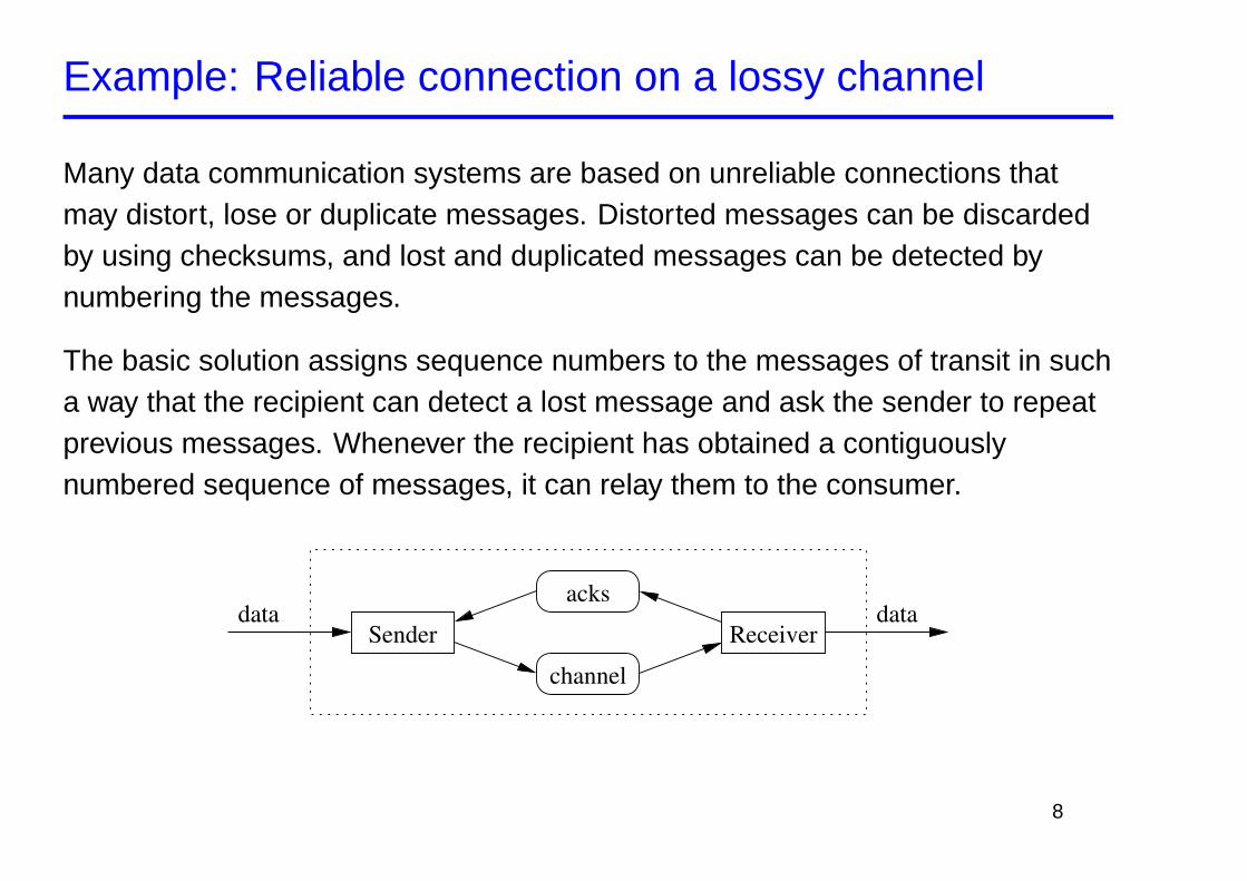
Many data communication systems are based on unreliable connections thatmay distort, lose or duplicate messages. Distorted messages can be discardedby using checksums, and lost and duplicated messages can be detected bynumbering the messages.
The basic solution assigns sequence numbers to the messages of transit in sucha way that the recipient can detect a lost message and ask the sender to repeatprevious messages. Whenever the recipient has obtained a contiguouslynumbered sequence of messages, it can relay them to the consumer.
dataSender
channel
acks
Receiverdata
8
Alternating bit protocol
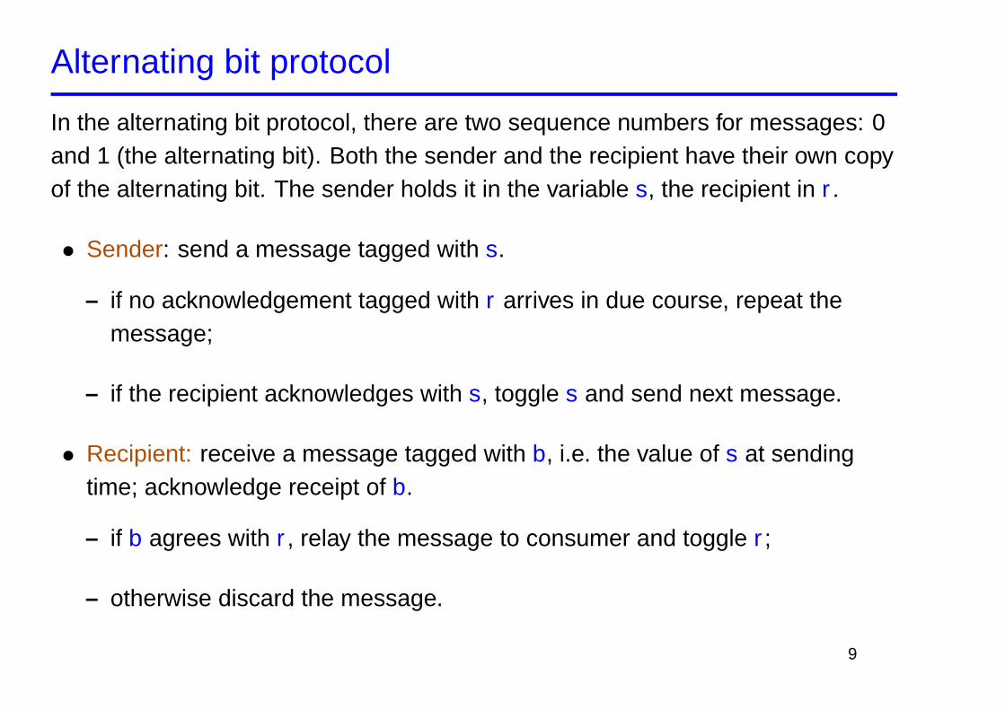
In the alternating bit protocol, there are two sequence numbers for messages: 0and 1 (the alternating bit). Both the sender and the recipient have their own copyof the alternating bit. The sender holds it in the variable s, the recipient in r .
• Sender: send a message tagged with s.
– if no acknowledgement tagged with r arrives in due course, repeat themessage;
– if the recipient acknowledges with s, toggle s and send next message.
• Recipient: receive a message tagged with b, i.e. the value of s at sendingtime; acknowledge receipt of b.
– if b agrees with r , relay the message to consumer and toggle r ;
– otherwise discard the message.
9
Alternating Bit protocol: Questions
Is the protocol correct?
Is every message eventually delivered, assuming that the channels are notpermanently faulty?
Are messages received in the right order?
Can two messages with the same alternating bit value be confused?
10
Alternating bit protocol: Communicating FA
s=0
s=1
?ack0 ?ack1
?ack1
?ack0
!msg0
!msg1
Senderaa0 a1
?ack0
!ack0
?ack1
!ack1
Acks channel
mm0 m1
?msg0
!msg0
?msg1
!msg1
Message channel
r=0
r=1
Receiver
?msg0 ?msg1
!ack1?msg1
!ack1!ack0
?msg0!ack0
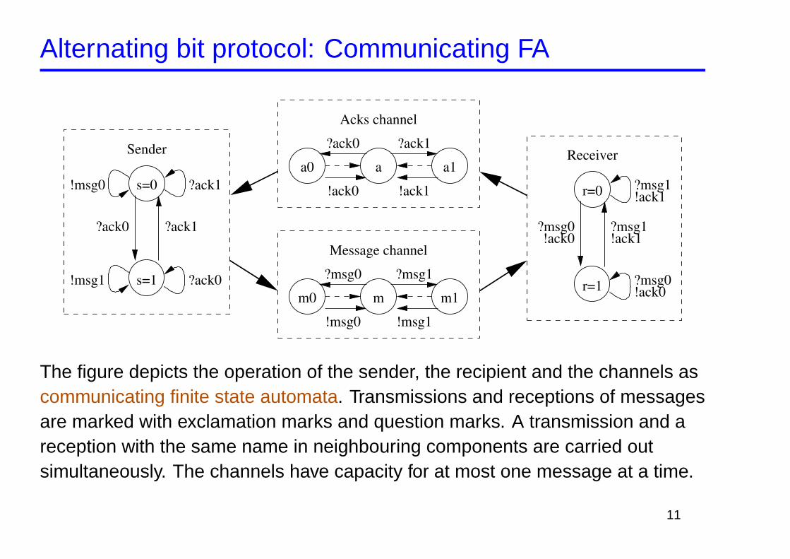
The figure depicts the operation of the sender, the recipient and the channels ascommunicating finite state automata. Transmissions and receptions of messagesare marked with exclamation marks and question marks. A transmission and areception with the same name in neighbouring components are carried outsimultaneously. The channels have capacity for at most one message at a time.
11
Alternating bit protocol: Petri net
����vs=0
����
s=1
����vm
����m1
����m0
����vr =0
����
r =1
����a1
����
a0
����v a
?ack0
?ack0
?ack1
?ack1
!msg1
!msg0
losemsg
losemsg
?msg0!ack
?msg1!ack
?msg0!ack0
?msg1!ack1
loseack
loseack
6?
6?
� -
� -
?
6
$
%
$
%��
?
6
� � � � �������������
AAAAAAAAAAAAU -
-
6
?
�� �
�� �
� -
� -
�
�
JJJJJJJJJJJ
�
� �� �� �
6
?
�
ZZZZ
ZZ}
������=
XXXXXXXX
XXXXXXXX
XXXXy
��������������������9
PPPPPPq
������1
������)
PPPPPPi
-
-
�
�
�
�
�
�
�
�
12
Alternating bit protocol: state space
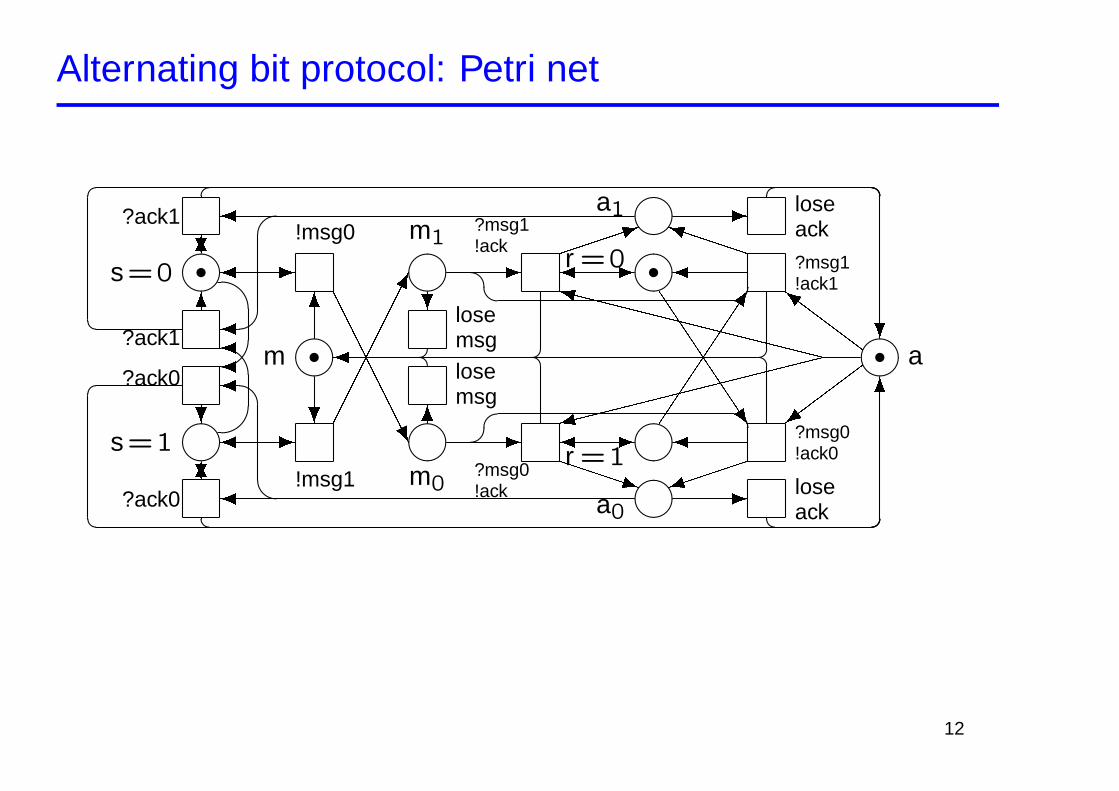
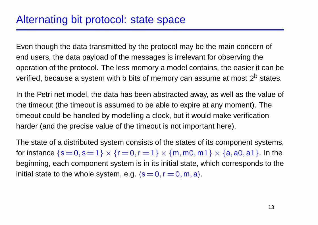
Even though the data transmitted by the protocol may be the main concern ofend users, the data payload of the messages is irrelevant for observing theoperation of the protocol. The less memory a model contains, the easier it can beverified, because a system with b bits of memory can assume at most 2b states.
In the Petri net model, the data has been abstracted away, as well as the value ofthe timeout (the timeout is assumed to be able to expire at any moment). Thetimeout could be handled by modelling a clock, but it would make verificationharder (and the precise value of the timeout is not important here).
The state of a distributed system consists of the states of its component systems,for instance {s=0, s=1} × {r =0, r =1} × {m, m0, m1} × {a, a0, a1}. In thebeginning, each component system is in its initial state, which corresponds to theinitial state to the whole system, e.g. 〈s=0, r =0, m, a〉.
13
Constructing the state space (idea)
The state of a Petri system is formed by the distribution of tokens in the places.
The state changes when enabled transitions are fired.
A transition is enabled if each of its pre-places contains a token.
When an enabled transition fires, a token is removed from each of its pre-placesand a token is inserted to each of its post-places.
14
The state space can be represented by a graph.
Nodes of the graph correspond to distributions of tokens.
Edges of the graph correspond to firing of transitions.
By constructing the state space, it is “fairly” easy to ensure that the alternating bitprotocol works. There are at most 2 · 2 · 3 · 3 = 36 states.
It turns out that from 〈s=0, r =0, m, a〉, there are 18 reachable nodes and 40edges.
15

Place/Transition Nets
16
Place/Transition Nets
Let us study Petri nets and their firing rule in more detail:
• A place may contain several tokens, which may be interpreted as resources.
• There may be several input and output arcs between a place and a transition.The number of these arcs is represented as the weight of a single arc.
• A transition is enabled if its each input place contains at least as many tokensas the corresponding input arc weight indicates.
• When an enabled transition is fired, its input arc weights are subtracted fromthe input place markings and its output arc weights are added to the outputplace markings.
17
Place/Transition Net
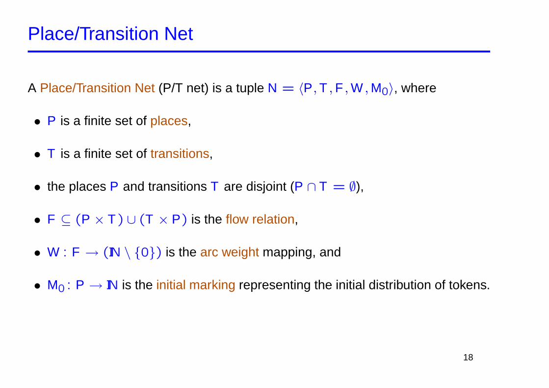
A Place/Transition Net (P/T net) is a tuple N = 〈P, T , F , W , M0〉, where
• P is a finite set of places,
• T is a finite set of transitions,
• the places P and transitions T are disjoint (P ∩ T = ∅),
• F ⊆ (P × T) ∪ (T × P) is the flow relation,
• W : F → (IN \ {0}) is the arc weight mapping, and
• M0 : P → IN is the initial marking representing the initial distribution of tokens.
18
P/T nets: Remarks
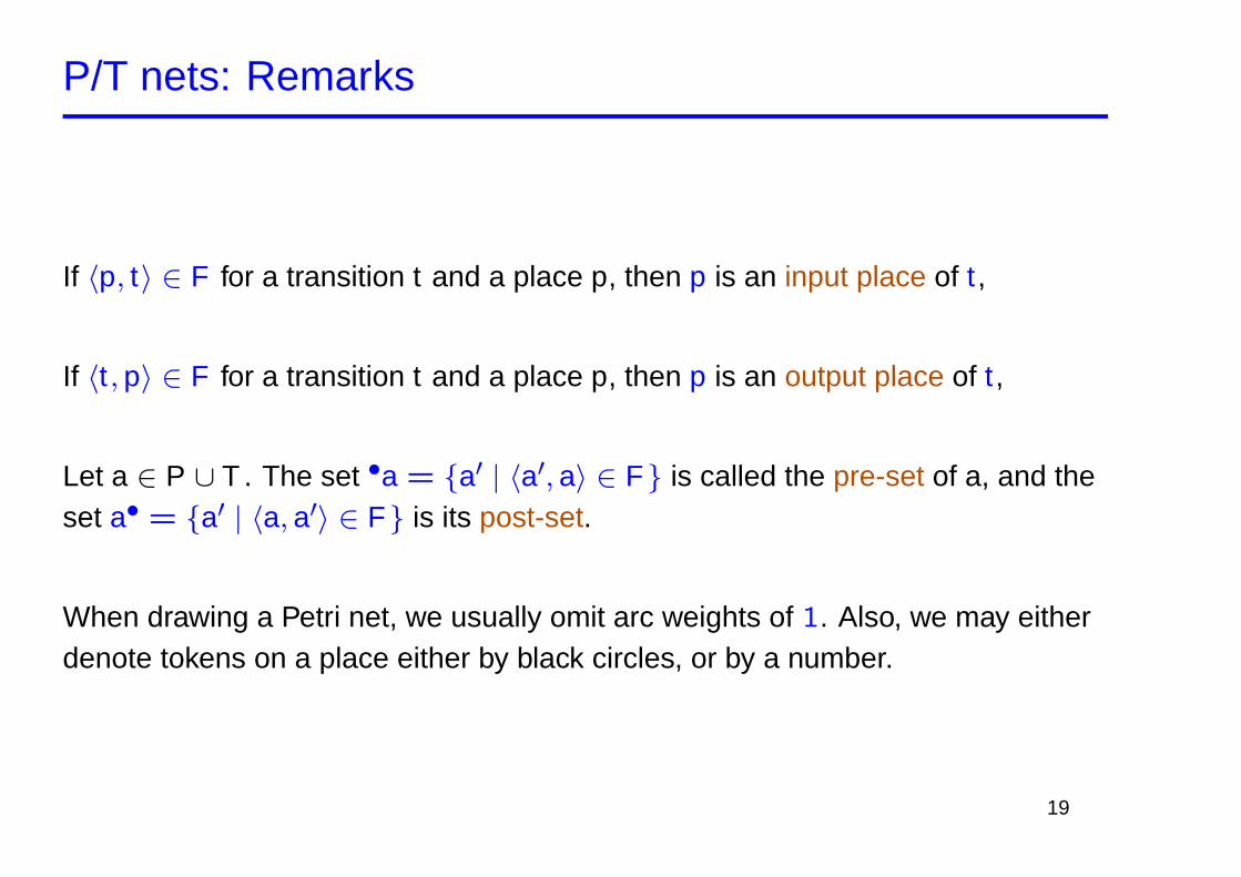
If 〈p, t〉 ∈ F for a transition t and a place p, then p is an input place of t ,
If 〈t , p〉 ∈ F for a transition t and a place p, then p is an output place of t ,
Let a ∈ P ∪ T . The set •a = {a′ | 〈a′, a〉 ∈ F} is called the pre-set of a, and theset a• = {a′ | 〈a, a′〉 ∈ F} is its post-set.
When drawing a Petri net, we usually omit arc weights of 1. Also, we may eitherdenote tokens on a place either by black circles, or by a number.
19
Alternative definitions
Sometimes the notation S (for Stellen) is used instead of P (for places) in thedefinition of Place/Transition nets.
Some definitions also use the notion of a place capacity (the maximum numberof tokens allowed in a place, possibly unbounded). Place capacities can besimulated by adding some additional places to the net (we will see how later),and thus for simplicity we will not define them in this course.
20
Place/Transition Net: Example
&%'$
p2
&%'$
p1
&%'$
p3
t
����
@@@R2
-2
vvv vv
v v
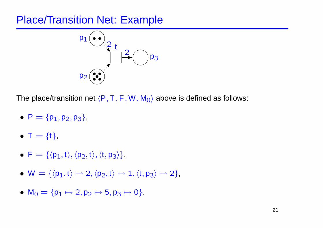
The place/transition net 〈P, T , F , W , M0〉 above is defined as follows:
• P = {p1, p2, p3},
• T = {t},
• F = {〈p1, t〉, 〈p2, t〉, 〈t , p3〉},
• W = {〈p1, t〉 7→ 2, 〈p2, t〉 7→ 1, 〈t , p3〉 7→ 2},
• M0 = {p1 7→ 2, p2 7→ 5, p3 7→ 0}.
21
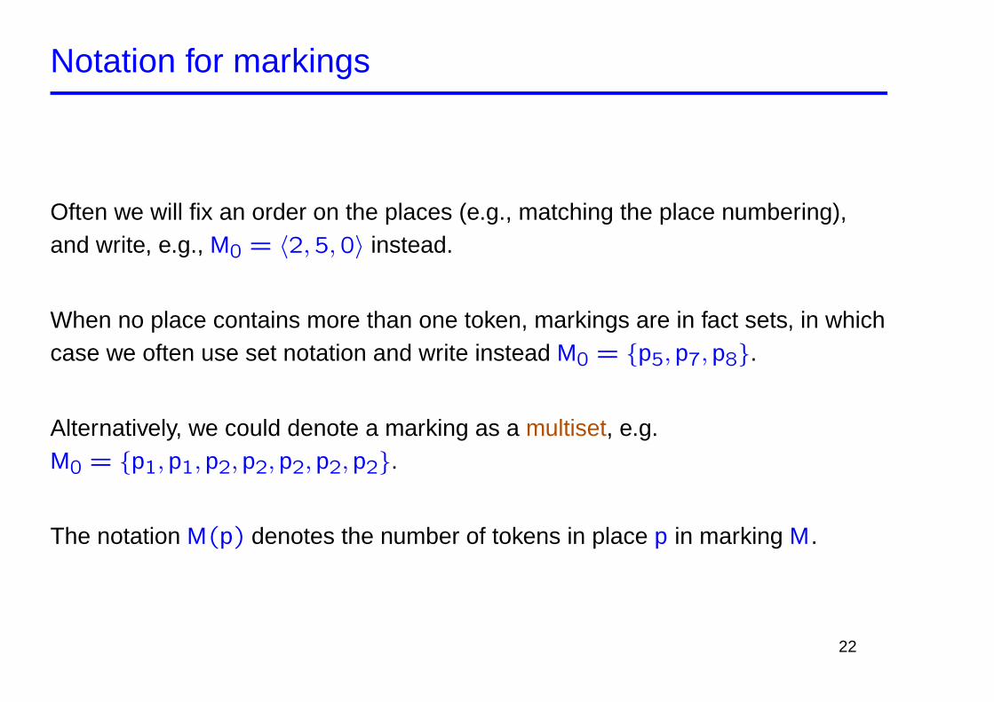
Notation for markings
Often we will fix an order on the places (e.g., matching the place numbering),and write, e.g., M0 = 〈2,5,0〉 instead.
When no place contains more than one token, markings are in fact sets, in whichcase we often use set notation and write instead M0 = {p5, p7, p8}.
Alternatively, we could denote a marking as a multiset, e.g.M0 = {p1, p1, p2, p2, p2, p2, p2}.
The notation M(p) denotes the number of tokens in place p in marking M.
22
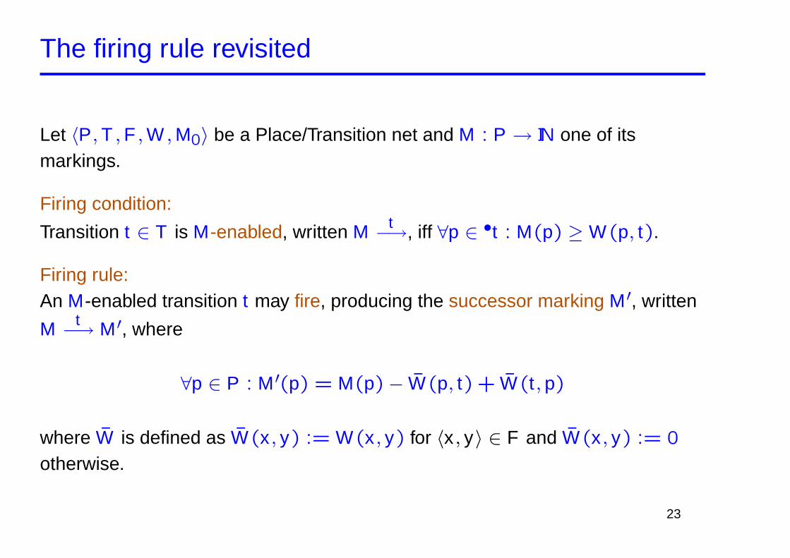
The firing rule revisited
Let 〈P, T , F , W , M0〉 be a Place/Transition net and M : P → IN one of itsmarkings.
Firing condition:
Transition t ∈ T is M-enabled, written M t−→, iff ∀p ∈ •t : M(p) ≥ W(p, t).
Firing rule:An M-enabled transition t may fire, producing the successor marking M ′, written
M t−→ M ′, where
∀p ∈ P : M ′(p) = M(p)− W(p, t) + W(t , p)
where W is defined as W(x , y) := W(x , y) for 〈x , y〉 ∈ F and W(x , y) := 0
otherwise.
23
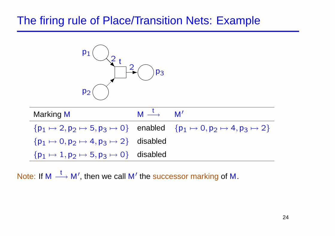
The firing rule of Place/Transition Nets: Example
&%'$
p2
&%'$
p1
&%'$
p3
t
����
@@@R2
-2
Marking M M t−→ M ′
{p1 7→ 2, p2 7→ 5, p3 7→ 0} enabled {p1 7→ 0, p2 7→ 4, p3 7→ 2}{p1 7→ 0, p2 7→ 4, p3 7→ 2} disabled
{p1 7→ 1, p2 7→ 5, p3 7→ 0} disabled
Note: If M t−→ M ′, then we call M ′ the successor marking of M.
24
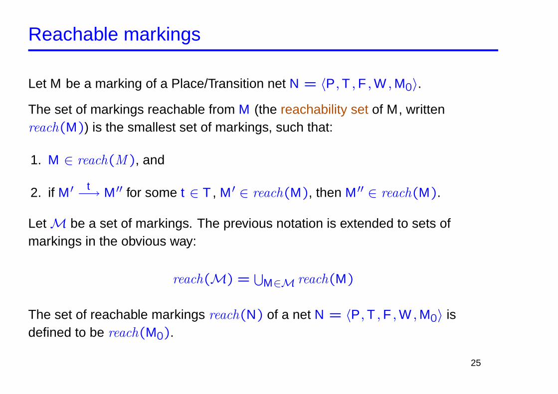
Reachable markings
Let M be a marking of a Place/Transition net N = 〈P, T , F , W , M0〉.
The set of markings reachable from M (the reachability set of M, writtenreach(M)) is the smallest set of markings, such that:
1. M ∈ reach(M ), and
2. if M ′ t−→ M ′′ for some t ∈ T , M ′ ∈ reach(M), then M ′′ ∈ reach(M).
Let M be a set of markings. The previous notation is extended to sets ofmarkings in the obvious way:
reach(M) =⋃
M∈M reach(M)
The set of reachable markings reach(N) of a net N = 〈P, T , F , W , M0〉 isdefined to be reach(M0).
25
Reachability Graph
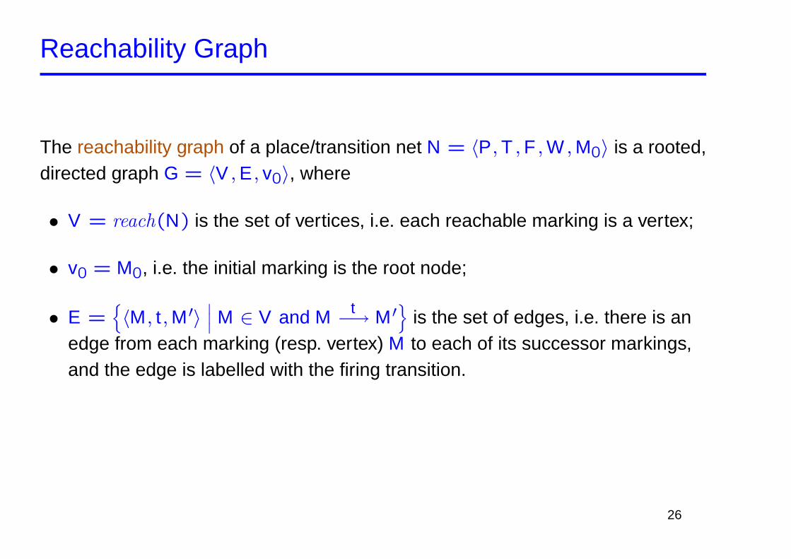
The reachability graph of a place/transition net N = 〈P, T , F , W , M0〉 is a rooted,directed graph G = 〈V , E , v0〉, where
• V = reach(N) is the set of vertices, i.e. each reachable marking is a vertex;
• v0 = M0, i.e. the initial marking is the root node;
• E ={〈M, t , M ′〉
∣∣∣ M ∈ V and M t−→ M ′}
is the set of edges, i.e. there is anedge from each marking (resp. vertex) M to each of its successor markings,and the edge is labelled with the firing transition.
26
Reachability Graph: Example
����
����
����
����
����
p1 p3 p5
p2 p4
t1 t3
t2
v
v
- - - -
- -
& $?
�������
�������
t1
t1
@@
@@
@@I
@@
@@
@@I
t2
t2�������
t3
> 〈1,1,0,0,0〉
〈1,0,0,1,0〉 〈0,1,1,0,0〉
〈0,0,1,1,0〉 〈0,0,0,0,1〉
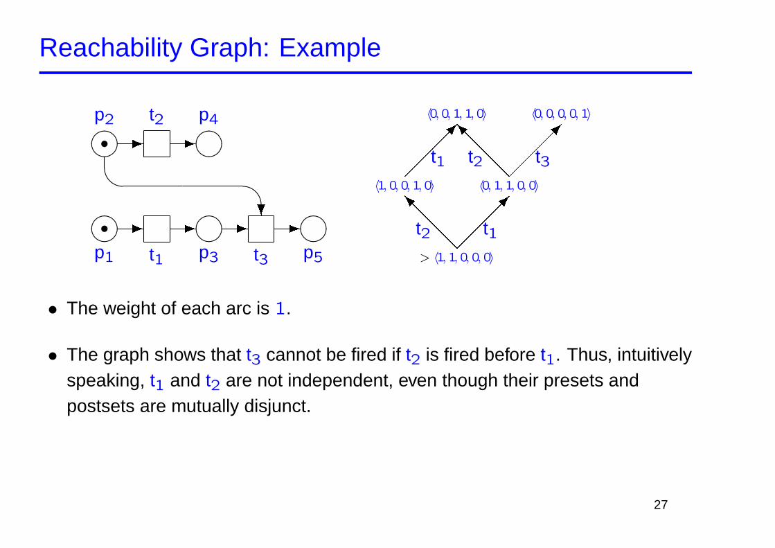
• The weight of each arc is 1.
• The graph shows that t3 cannot be fired if t2 is fired before t1. Thus, intuitivelyspeaking, t1 and t2 are not independent, even though their presets andpostsets are mutually disjunct.
27
Computing the reachability graph
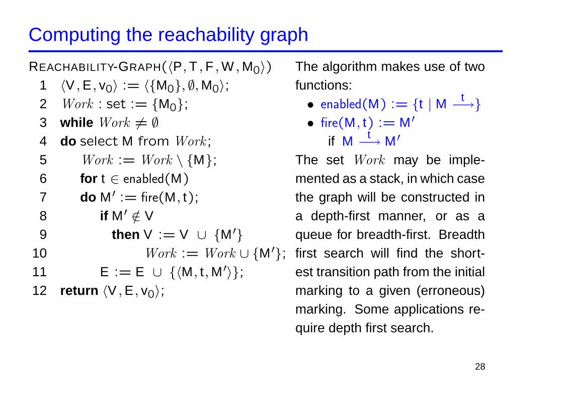
REACHABILITY-GRAPH(〈P, T , F , W , M0〉)1 〈V , E , v0〉 := 〈{M0}, ∅, M0〉;2 Work : set := {M0};3 while Work 6= ∅4 do select M from Work ;
5 Work := Work \ {M};6 for t ∈ enabled(M)
7 do M ′ := fire(M, t);8 if M ′ /∈ V9 then V := V ∪ {M ′}
10 Work := Work ∪ {M ′};11 E := E ∪ {〈M, t , M ′〉};12 return 〈V , E , v0〉;
The algorithm makes use of twofunctions:• enabled(M) := {t | M t−→}• fire(M, t) := M ′
if M t−→ M ′
The set Work may be imple-mented as a stack, in which casethe graph will be constructed ina depth-first manner, or as aqueue for breadth-first. Breadthfirst search will find the short-est transition path from the initialmarking to a given (erroneous)marking. Some applications re-quire depth first search.
28
The size of the reachability graph
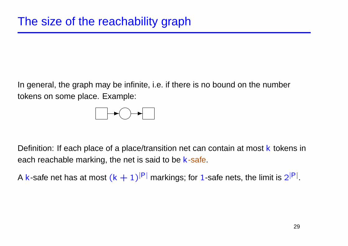
In general, the graph may be infinite, i.e. if there is no bound on the numbertokens on some place. Example:
- -����
Definition: If each place of a place/transition net can contain at most k tokens ineach reachable marking, the net is said to be k -safe.
A k -safe net has at most (k + 1)|P| markings; for 1-safe nets, the limit is 2|P|.
29
Use of reachability graphs
In practice, all analysis tools and methods for Petri nets compute the reachabilitygraph in some way or other. The reachability graph can be effectively computedif the net is k -safe for some k .
If the net is not k -safe for any k , we may compute the coverability graph (seenext lecture).
30
Analysis with Place/Transition Nets
31
Recap from last Session
We discussed the following topics:
Modeling: Petri nets (and others)
Specifying: reachability (and others, mostly informally)
Verifying: construction of reachability graph
32
Programme
Example: modeling, specifying, and reachability analysis
Coverability graphs
Analysis with reachability and coverability graphs
33
Example: A logical puzzle
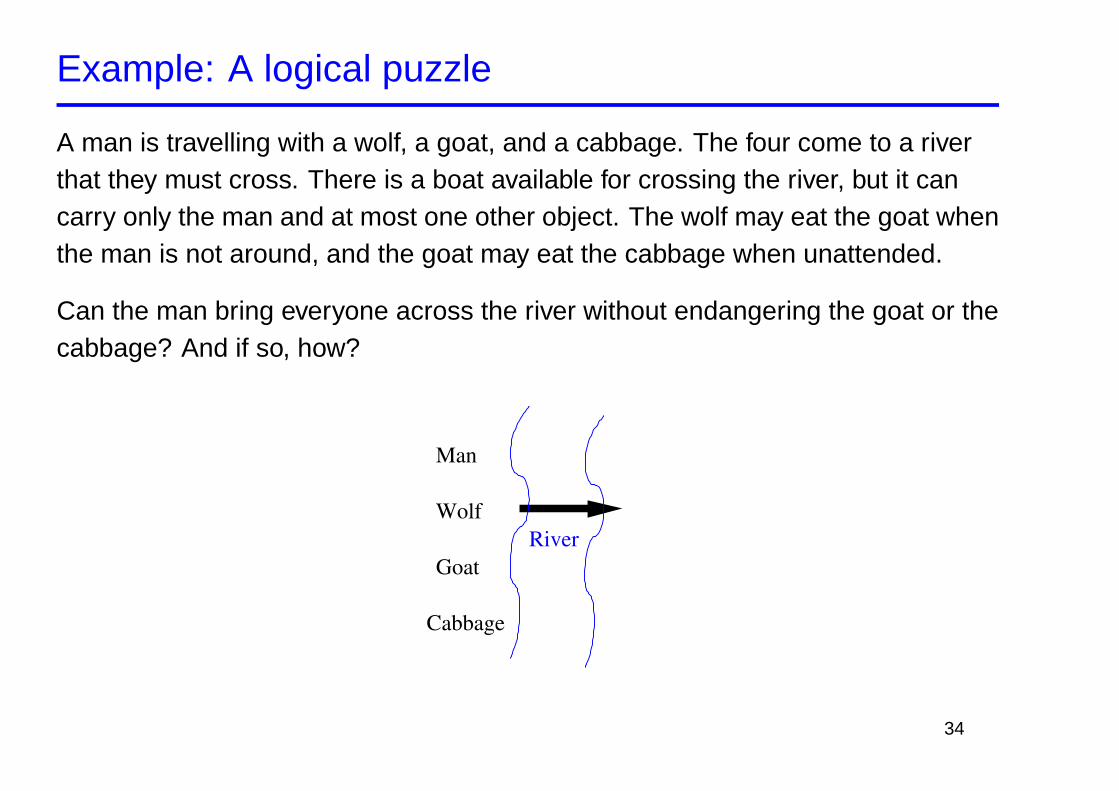
A man is travelling with a wolf, a goat, and a cabbage. The four come to a riverthat they must cross. There is a boat available for crossing the river, but it cancarry only the man and at most one other object. The wolf may eat the goat whenthe man is not around, and the goat may eat the cabbage when unattended.
Can the man bring everyone across the river without endangering the goat or thecabbage? And if so, how?
Cabbage
Goat
Wolf
Man
River
34
Example: Modeling
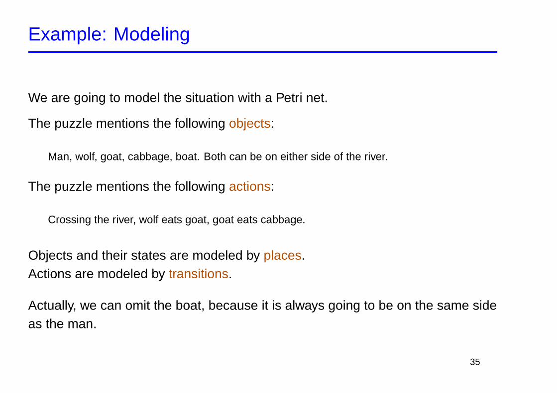
We are going to model the situation with a Petri net.
The puzzle mentions the following objects:
Man, wolf, goat, cabbage, boat. Both can be on either side of the river.
The puzzle mentions the following actions:
Crossing the river, wolf eats goat, goat eats cabbage.
Objects and their states are modeled by places.Actions are modeled by transitions.
Actually, we can omit the boat, because it is always going to be on the same sideas the man.
35
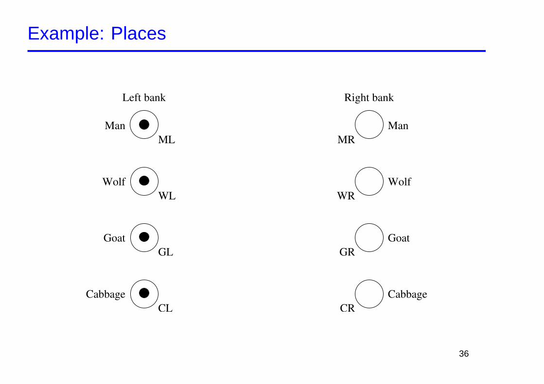
Example: Places
Man
Wolf
Goat
Cabbage
Left bank
CL
GL
WL
ML
Right bank
Wolf
Goat
Cabbage
ManMR
WR
GR
CR
36
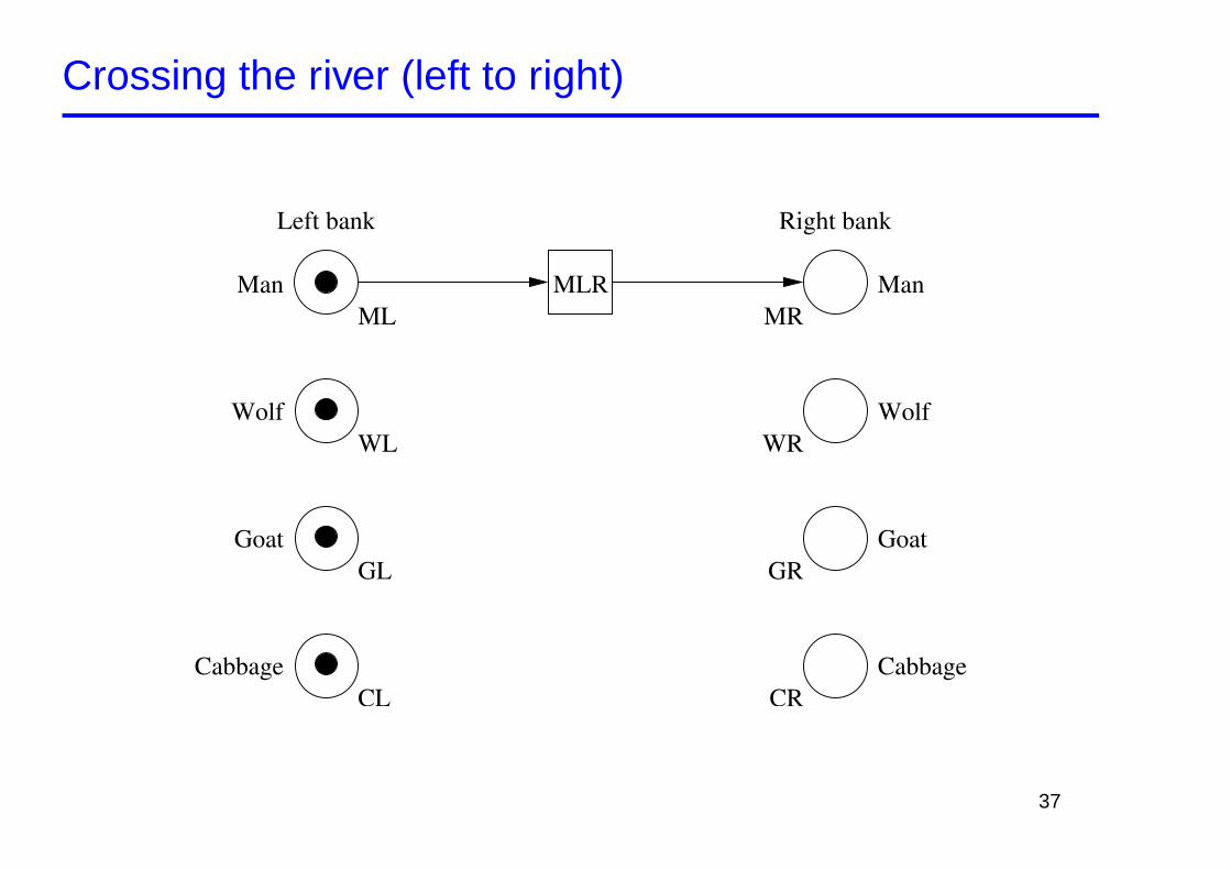
Crossing the river (left to right)
Man
Wolf
Goat
Cabbage
Left bank
CL
GL
WL
ML
Right bank
Wolf
Goat
Cabbage
ManMR
WR
GR
CR
MLR
37
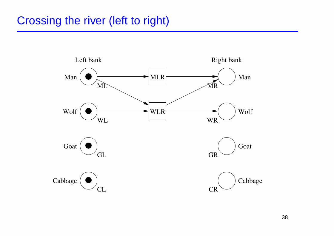
Crossing the river (left to right)
Man
Wolf
Goat
Cabbage
Left bank
CL
GL
WL
ML
Right bank
Wolf
Goat
Cabbage
ManMR
WR
GR
CR
WLR
MLR
38
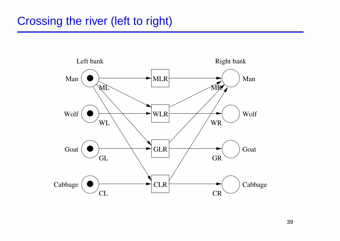
Crossing the river (left to right)
Man
Wolf
Goat
Cabbage
Left bank
CL
GL
WL
ML
Right bank
Wolf
Goat
Cabbage
ManMR
WR
GR
CR
WLR
MLR
CLR
GLR
39
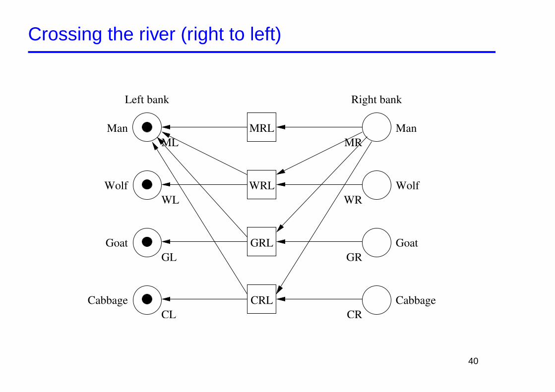
Crossing the river (right to left)
Man
Wolf
Goat
Cabbage
Left bank
CL
GL
WL
ML
Right bank
Wolf
Goat
Cabbage
ManMR
WR
GR
CR
WRL
MRL
CRL
GRL
40
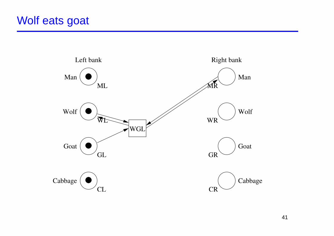
Wolf eats goat
Man
Wolf
Goat
Cabbage
Left bank
CL
GL
Right bank
Wolf
Goat
Cabbage
ManMR
WR
GR
CR
WL
ML
WGL
41
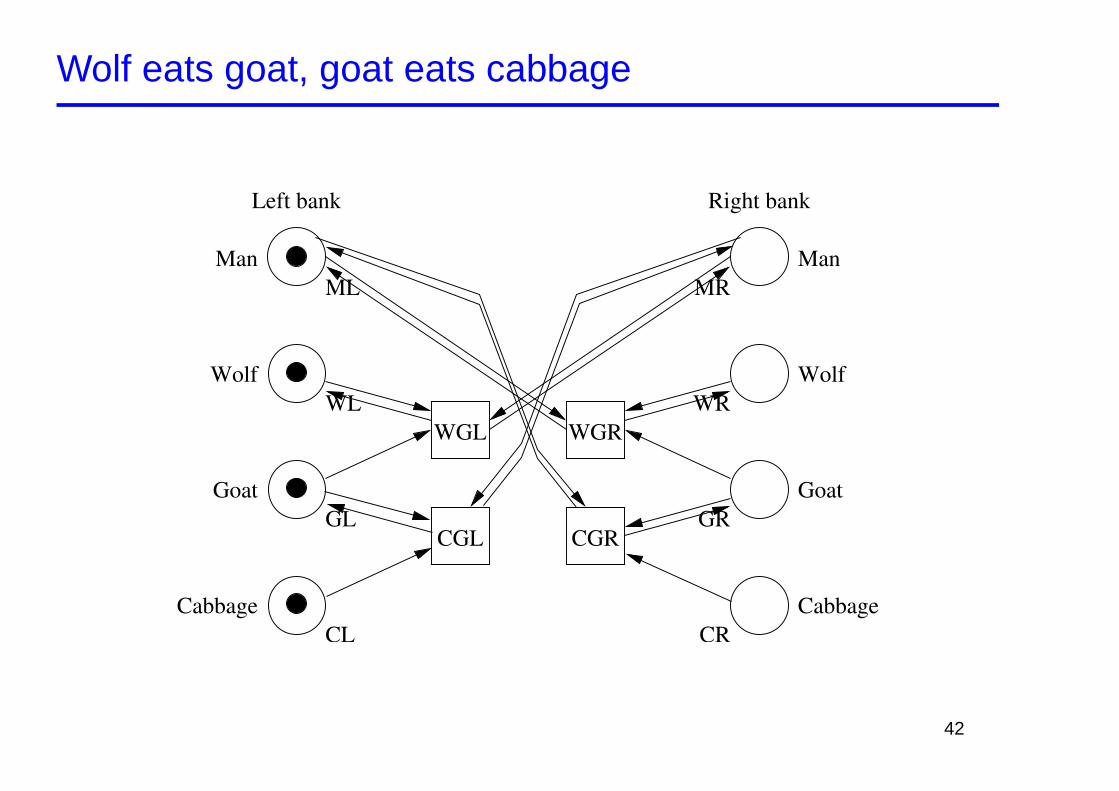
Wolf eats goat, goat eats cabbage
Man
Wolf
Goat
Cabbage
Left bank
CL
GL
Right bank
Wolf
Goat
Cabbage
ManMR
WR
GR
CR
WL
ML
WGL WGR
CGL CGR
42
Example: Specification
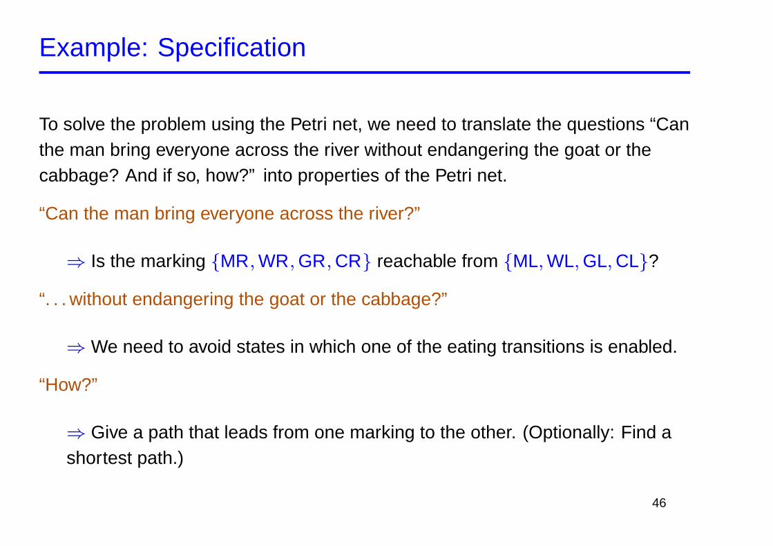
To solve the problem using the Petri net, we need to translate the questions “Canthe man bring everyone across the river without endangering the goat or thecabbage? And if so, how?” into properties of the Petri net.
“Can the man bring everyone across the river?”
⇒ Is the marking {MR, WR, GR, CR} reachable from {ML, WL, GL, CL}?
“. . . without endangering the goat or the cabbage?”
⇒ We need to avoid states in which one of the eating transitions is enabled.
“How?”
⇒ Give a path that leads from one marking to the other. (Optionally: Findshortest path.)
43
Example: Specification
To solve the problem using the Petri net, we need to translate the questions “Canthe man bring everyone across the river without endangering the goat or thecabbage? And if so, how?” into properties of the Petri net.
“Can the man bring everyone across the river?”
⇒ Is the marking {MR, WR, GR, CR} reachable from {ML, WL, GL, CL}?
“. . . without endangering the goat or the cabbage?”
⇒ We need to avoid states in which one of the eating transitions is enabled.
“How?”
⇒ Give a path that leads from one marking to the other. (Optionally: Findshortest path.)
44
Example: Specification
To solve the problem using the Petri net, we need to translate the questions “Canthe man bring everyone across the river without endangering the goat or thecabbage? And if so, how?” into properties of the Petri net.
“Can the man bring everyone across the river?”
⇒ Is the marking {MR, WR, GR, CR} reachable from {ML, WL, GL, CL}?
“. . . without endangering the goat or the cabbage?”
⇒ We need to avoid states in which one of the eating transitions is enabled.
“How?”
⇒ Give a path that leads from one marking to the other. (Optionally: Find ashortest path.)
45
Example: Specification
To solve the problem using the Petri net, we need to translate the questions “Canthe man bring everyone across the river without endangering the goat or thecabbage? And if so, how?” into properties of the Petri net.
“Can the man bring everyone across the river?”
⇒ Is the marking {MR, WR, GR, CR} reachable from {ML, WL, GL, CL}?
“. . . without endangering the goat or the cabbage?”
⇒ We need to avoid states in which one of the eating transitions is enabled.
“How?”
⇒ Give a path that leads from one marking to the other. (Optionally: Find ashortest path.)
46
Result
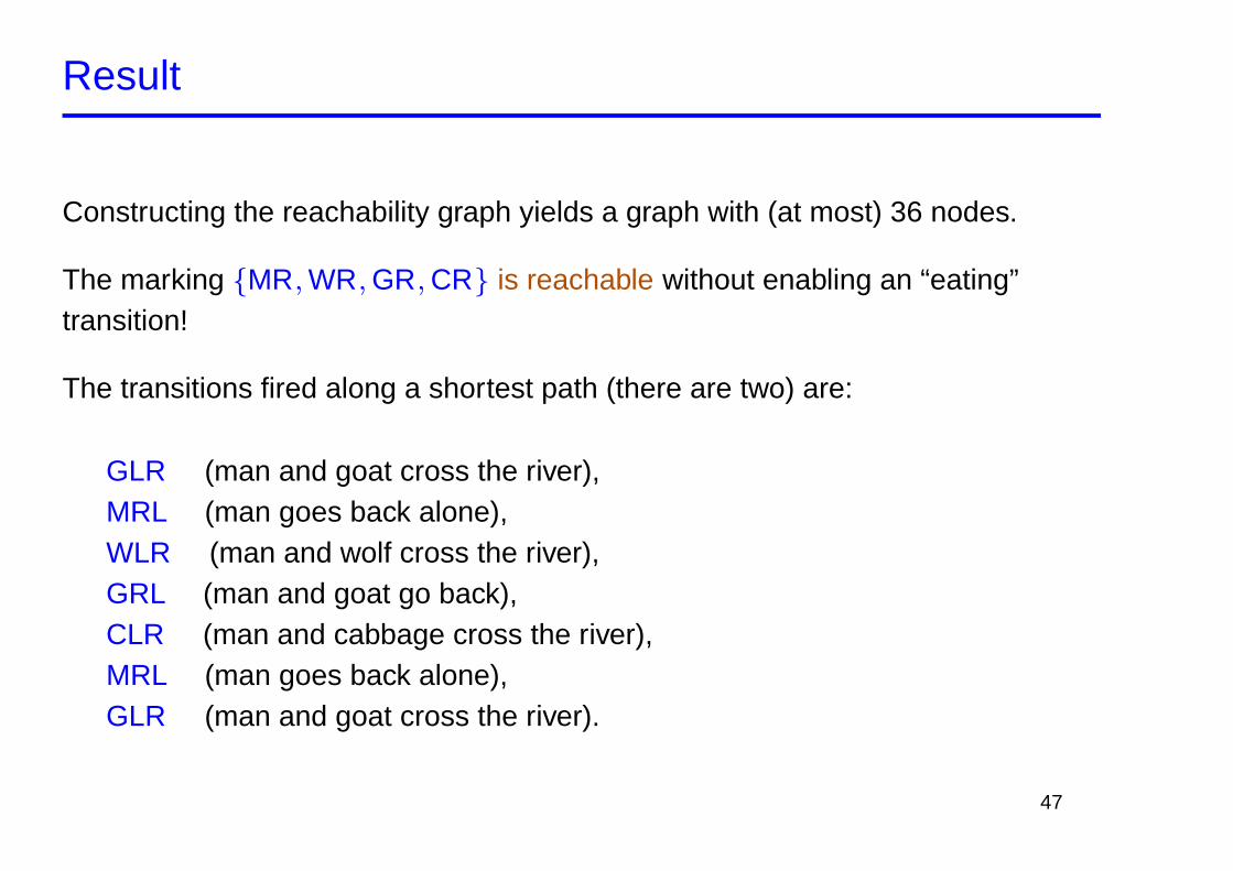
Constructing the reachability graph yields a graph with (at most) 36 nodes.
The marking {MR, WR, GR, CR} is reachable without enabling an “eating”transition!
The transitions fired along a shortest path (there are two) are:
GLR (man and goat cross the river),MRL (man goes back alone),WLR (man and wolf cross the river),GRL (man and goat go back),CLR (man and cabbage cross the river),MRL (man goes back alone),GLR (man and goat cross the river).
47
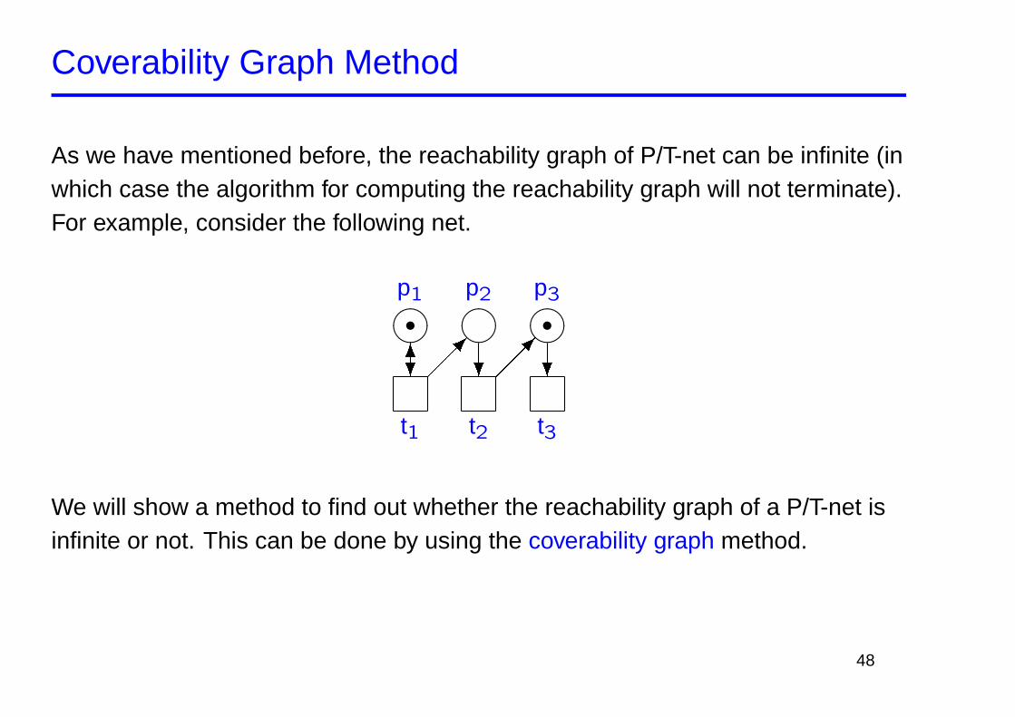
Coverability Graph Method
As we have mentioned before, the reachability graph of P/T-net can be infinite (inwhich case the algorithm for computing the reachability graph will not terminate).For example, consider the following net.
t1 t2 t3
����
����
����p1 p2 p3
v v? ? ?6�����
�����
We will show a method to find out whether the reachability graph of a P/T-net isinfinite or not. This can be done by using the coverability graph method.
48
ω-Markings
First we introduce a new symbol ω to represent “arbitrarily many” tokens.
We extend the arithmetic on natural numbers with ω as follows. For all n ∈ IN:n + ω = ω + n = ω,ω + ω = ω,ω − n = ω,0 · ω = 0, ω · ω = ω,n ≥ 1 ⇒ n · ω = ω · n = ω,n ≤ ω, and ω ≤ ω.
Note: ω − ω remains undefined, but we will not need it.
We will extend the notion of markings to ω-markings. In an ω-marking, eachplace p will either have n ∈ IN tokens, or ω tokens (infinitely many).
49
Firing Rule and ω-markings
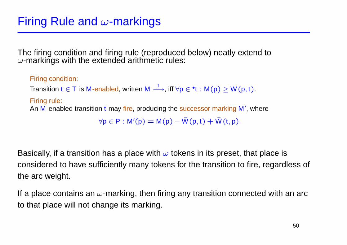
The firing condition and firing rule (reproduced below) neatly extend toω-markings with the extended arithmetic rules:
Firing condition:
Transition t ∈ T is M-enabled, written Mt−→, iff ∀p ∈ •t : M(p) ≥ W(p, t).
Firing rule:An M-enabled transition t may fire, producing the successor marking M ′, where
∀p ∈ P : M ′(p) = M(p)− W(p, t) + W(t , p).
Basically, if a transition has a place with ω tokens in its preset, that place isconsidered to have sufficiently many tokens for the transition to fire, regardless ofthe arc weight.
If a place contains an ω-marking, then firing any transition connected with an arcto that place will not change its marking.
50

Definition of Covering
An ω-marking M ′ covers an ω-marking M, denoted M ≤ M ′, iff
∀p ∈ P : M(p) ≤ M ′(p).
An ω-marking M ′ strictly covers an ω-marking M, denoted M < M ′, iff
M ≤ M ′ and M ′ 6= M.
51
Coverability and Transition Sequences (1/2)
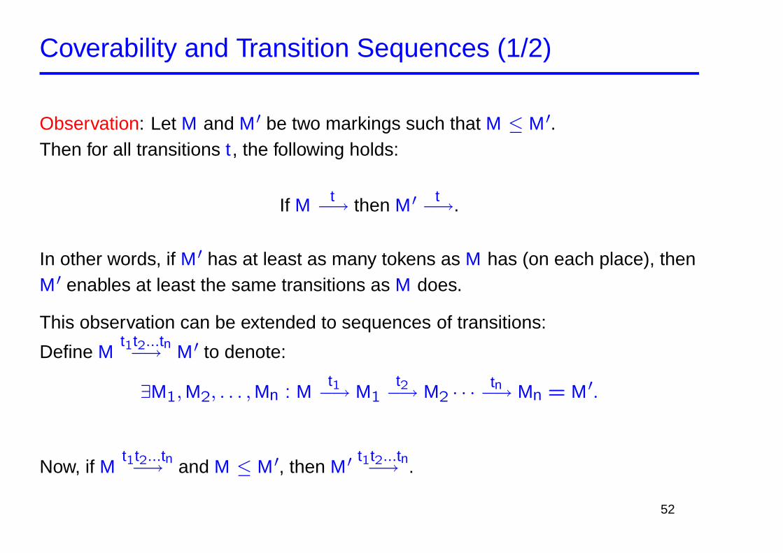
Observation: Let M and M ′ be two markings such that M ≤ M ′.Then for all transitions t , the following holds:
If M t−→ then M ′ t−→.
In other words, if M ′ has at least as many tokens as M has (on each place), thenM ′ enables at least the same transitions as M does.
This observation can be extended to sequences of transitions:
Define Mt1t2...tn−→ M ′ to denote:
∃M1, M2, . . . , Mn : Mt1−→ M1
t2−→ M2 · · ·tn−→ Mn = M ′.
Now, if Mt1t2...tn−→ and M ≤ M ′, then M ′ t1t2...tn−→ .
52
Coverability and Transition Sequences (2/2)
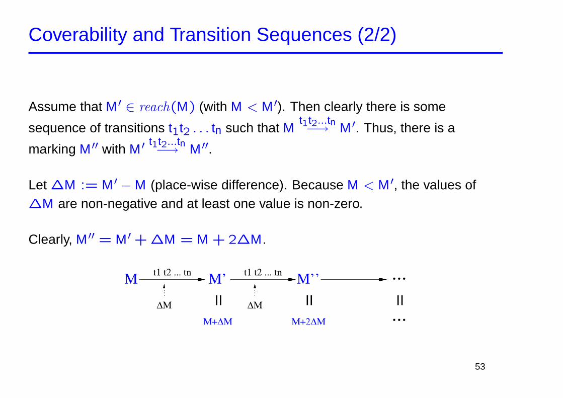
Assume that M ′ ∈ reach(M) (with M < M ′). Then clearly there is some
sequence of transitions t1t2 . . . tn such that Mt1t2...tn−→ M ′. Thus, there is a
marking M ′′ with M ′ t1t2...tn−→ M ′′.
Let ∆M := M ′ − M (place-wise difference). Because M < M ′, the values of∆M are non-negative and at least one value is non-zero.
Clearly, M ′′ = M ′ + ∆M = M + 2∆M.
M t1 t2 ... tn M’ t1 t2 ... tn M’’= =
∆Μ ∆Μ
Μ+∆Μ Μ+2∆Μ
...
=
...
53
By firing the transition sequence t1t2 . . . tn repeatedly we can “pump” an arbitrarynumber of tokens to all the places having a non-zero marking in ∆M.
The basic idea for constructing the coverability graph is now to replace themarking M ′ with a marking where all the places with non-zero tokens in ∆M arereplaced by ω.
54
Coverability Graph Algorithm (1/2)
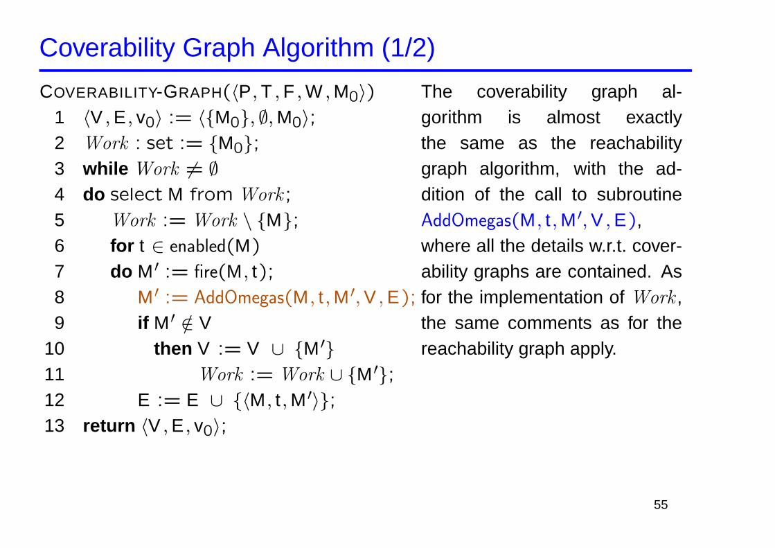
COVERABILITY-GRAPH(〈P, T , F , W , M0〉)1 〈V , E , v0〉 := 〈{M0}, ∅, M0〉;2 Work : set := {M0};3 while Work 6= ∅4 do select M from Work ;
5 Work := Work \ {M};6 for t ∈ enabled(M)
7 do M ′ := fire(M, t);8 M ′ := AddOmegas(M, t , M ′, V , E);
9 if M ′ /∈ V10 then V := V ∪ {M ′}11 Work := Work ∪ {M ′};12 E := E ∪ {〈M, t , M ′〉};13 return 〈V , E , v0〉;
The coverability graph al-gorithm is almost exactlythe same as the reachabilitygraph algorithm, with the ad-dition of the call to subroutineAddOmegas(M, t , M ′, V , E),where all the details w.r.t. cover-ability graphs are contained. Asfor the implementation of Work ,the same comments as for thereachability graph apply.
55
Coverability Graph Algorithm (2/2)
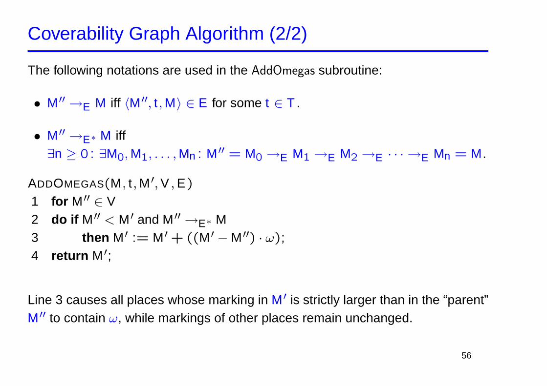
The following notations are used in the AddOmegas subroutine:
• M ′′ →E M iff 〈M ′′, t , M〉 ∈ E for some t ∈ T .
• M ′′ →E∗ M iff∃n ≥ 0: ∃M0, M1, . . . , Mn : M ′′ = M0 →E M1 →E M2 →E · · · →E Mn = M.
ADDOMEGAS(M, t , M ′, V , E)
1 for M ′′ ∈ V2 do if M ′′ < M ′ and M ′′ →E∗ M3 then M ′ := M ′ + ((M ′ − M ′′) · ω);
4 return M ′;
Line 3 causes all places whose marking in M ′ is strictly larger than in the “parent”M ′′ to contain ω, while markings of other places remain unchanged.
56
Termination of the Coverability Graph Algorithm (1/2)
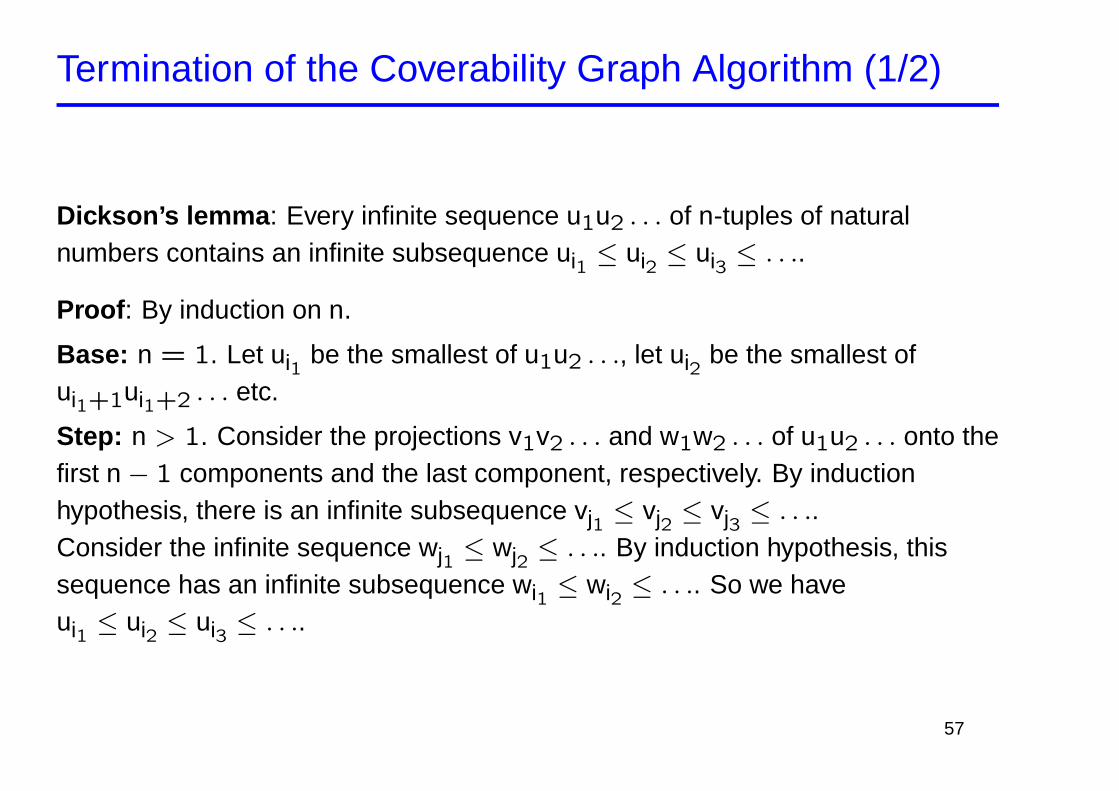
Dickson’s lemma : Every infinite sequence u1u2 . . . of n-tuples of naturalnumbers contains an infinite subsequence ui1 ≤ ui2 ≤ ui3 ≤ . . ..
Proof : By induction on n.
Base: n = 1. Let ui1 be the smallest of u1u2 . . ., let ui2 be the smallest ofui1+1ui1+2 . . . etc.
Step: n > 1. Consider the projections v1v2 . . . and w1w2 . . . of u1u2 . . . onto thefirst n − 1 components and the last component, respectively. By inductionhypothesis, there is an infinite subsequence vj1 ≤ vj2 ≤ vj3 ≤ . . ..Consider the infinite sequence wj1 ≤ wj2 ≤ . . .. By induction hypothesis, thissequence has an infinite subsequence wi1 ≤ wi2 ≤ . . .. So we haveui1 ≤ ui2 ≤ ui3 ≤ . . ..
57
Termination of the Coverability Graph Algorithm (2/2)
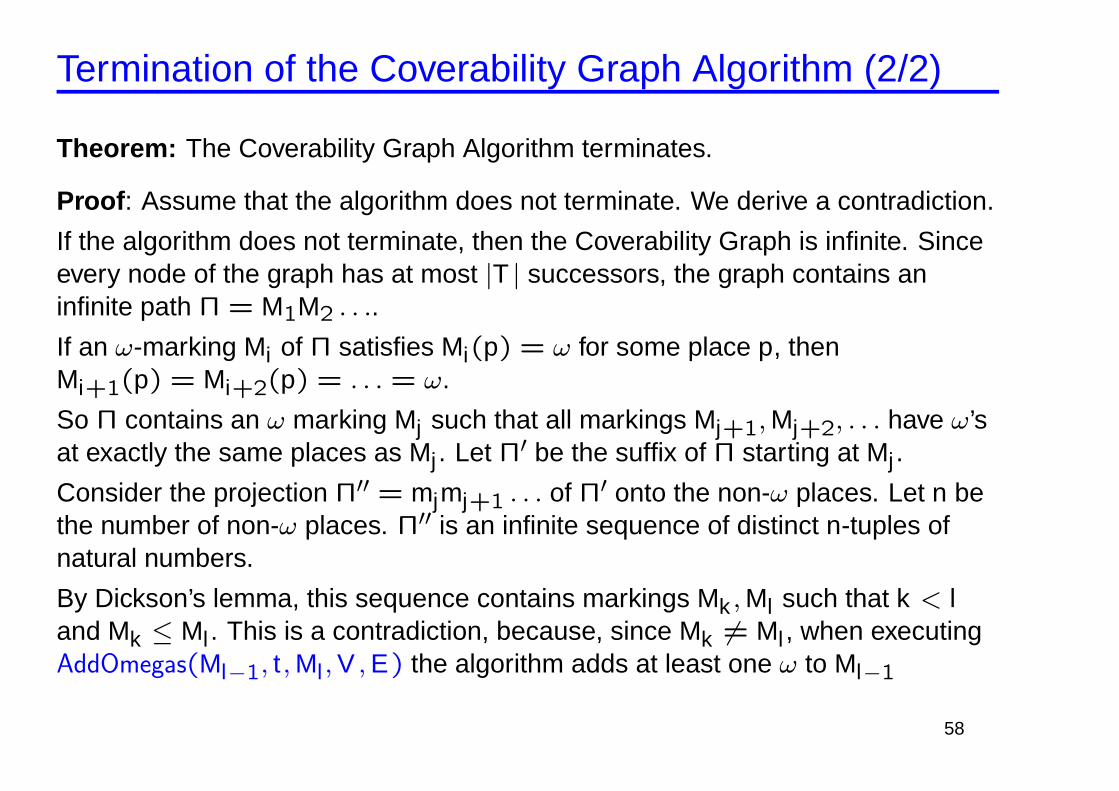
Theorem: The Coverability Graph Algorithm terminates.
Proof : Assume that the algorithm does not terminate. We derive a contradiction.
If the algorithm does not terminate, then the Coverability Graph is infinite. Sinceevery node of the graph has at most |T | successors, the graph contains aninfinite path Π = M1M2 . . ..
If an ω-marking Mi of Π satisfies Mi(p) = ω for some place p, thenMi+1(p) = Mi+2(p) = . . . = ω.
So Π contains an ω marking Mj such that all markings Mj+1, Mj+2, . . . have ω’sat exactly the same places as Mj . Let Π′ be the suffix of Π starting at Mj .
Consider the projection Π′′ = mjmj+1 . . . of Π′ onto the non-ω places. Let n bethe number of non-ω places. Π′′ is an infinite sequence of distinct n-tuples ofnatural numbers.
By Dickson’s lemma, this sequence contains markings Mk , Ml such that k < land Mk ≤ Ml . This is a contradiction, because, since Mk 6= Ml , when executingAddOmegas(Ml−1, t , Ml , V , E) the algorithm adds at least one ω to Ml−1
58
Remarks on the Coverability Graph Algorithm
If the reachability graph is finite, the algorithm AddOmegas(M, t , M ′, V , E) willalways return M ′ as its output (i.e., the third parameter).
In this case the coverability graph algorithm will return the reachability graph (butit will run more slowly).
Implementations of the algorithm are bound to be slow because of the for loop inAddOmegas, which has to traverse the potentially large size of the graph.
The result of the algorithm is not unique, e.g. it depends on the implementationof Work and on the exact order of fired transitions on line 5 of the main routine.
59
Example 1: Coverability Graph
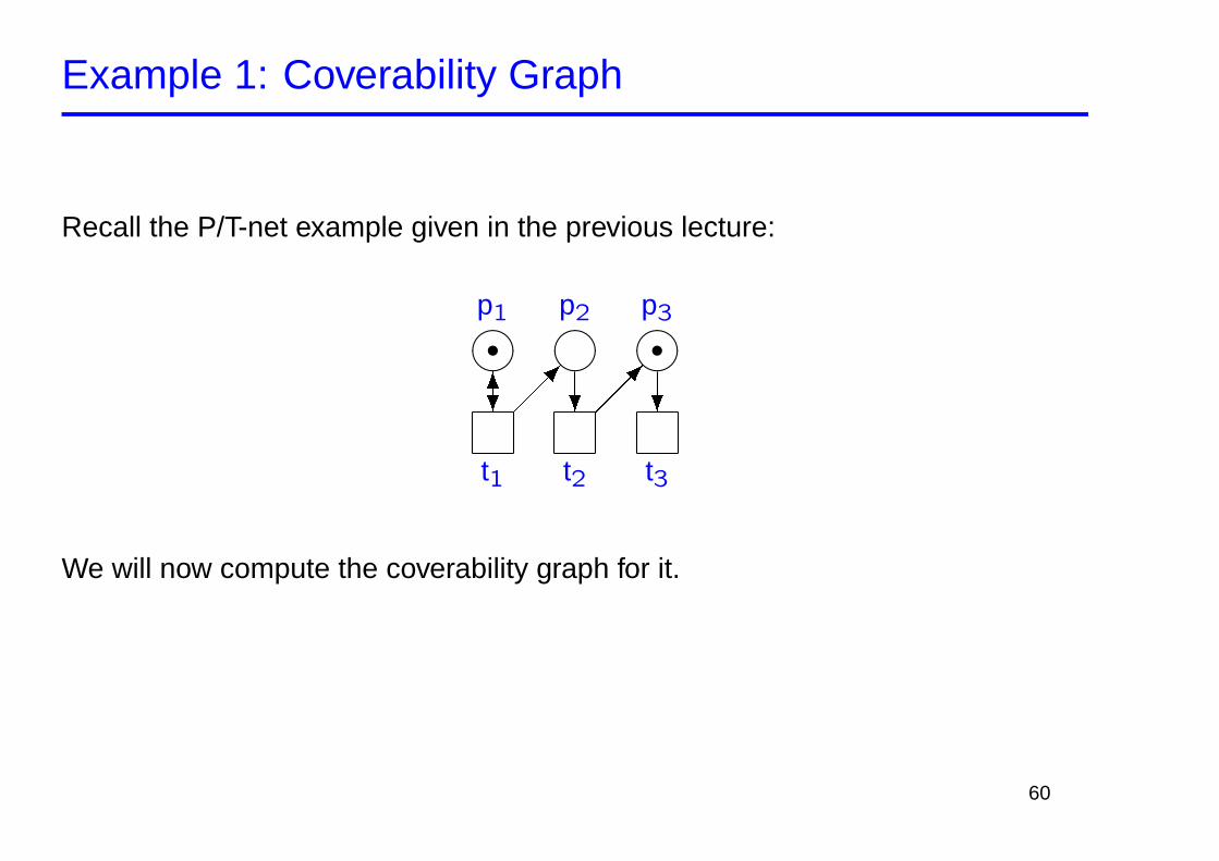
Recall the P/T-net example given in the previous lecture:
t1 t2 t3
����
����
����p1 p2 p3
v v? ? ?6�����
�����
We will now compute the coverability graph for it.
60
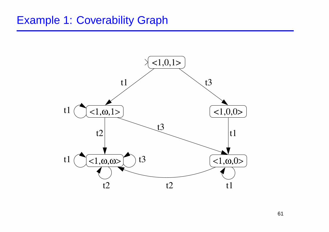
Example 1: Coverability Graph
t2 t1
t3t1
t1
t1
t3
t3
t2 t1
<1,0,1>
<1,0,0>
t2
<1,ω,1>
<1,ω,ω> <1,ω,0>
61
Example 2
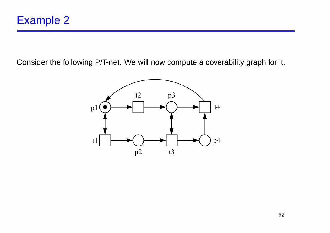
Consider the following P/T-net. We will now compute a coverability graph for it.
t4
p4
p1
t1
p2 t3
p3t2
62
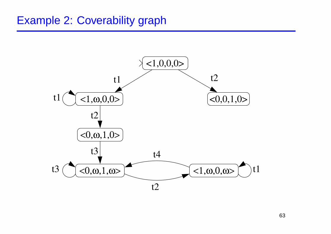
Example 2: Coverability graph
<1,0,0,0>
t1 t2
t2
t3
t1
t2
t4
t1
t3
<0,0,1,0><1,ω,0,0>
<0,ω,1,0>
<0,ω,1,ω> <1,ω,0,ω>
63
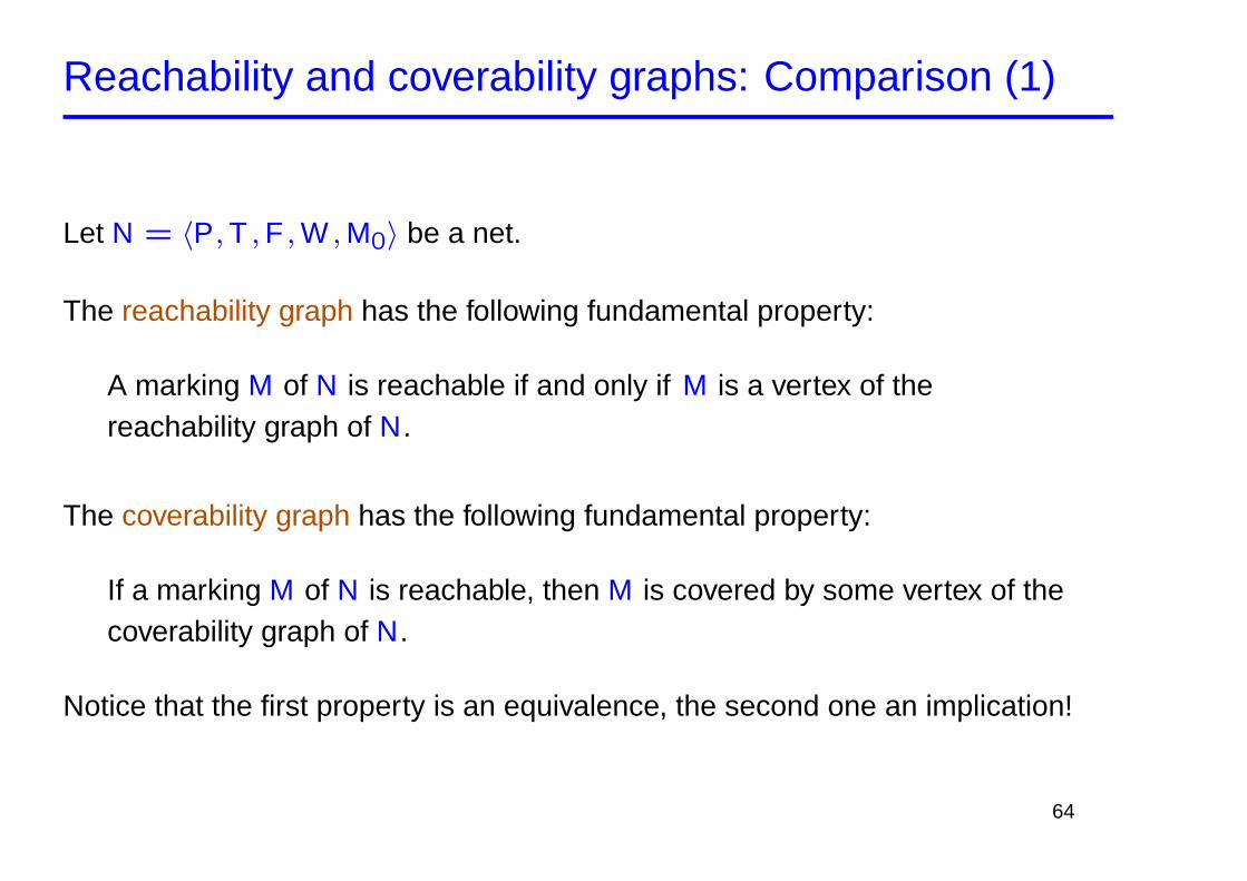
Reachability and coverability graphs: Comparison (1)
Let N = 〈P, T , F , W , M0〉 be a net.
The reachability graph has the following fundamental property:
A marking M of N is reachable if and only if M is a vertex of thereachability graph of N.
The coverability graph has the following fundamental property:
If a marking M of N is reachable, then M is covered by some vertex of thecoverability graph of N.
Notice that the first property is an equivalence, the second one an implication!
64
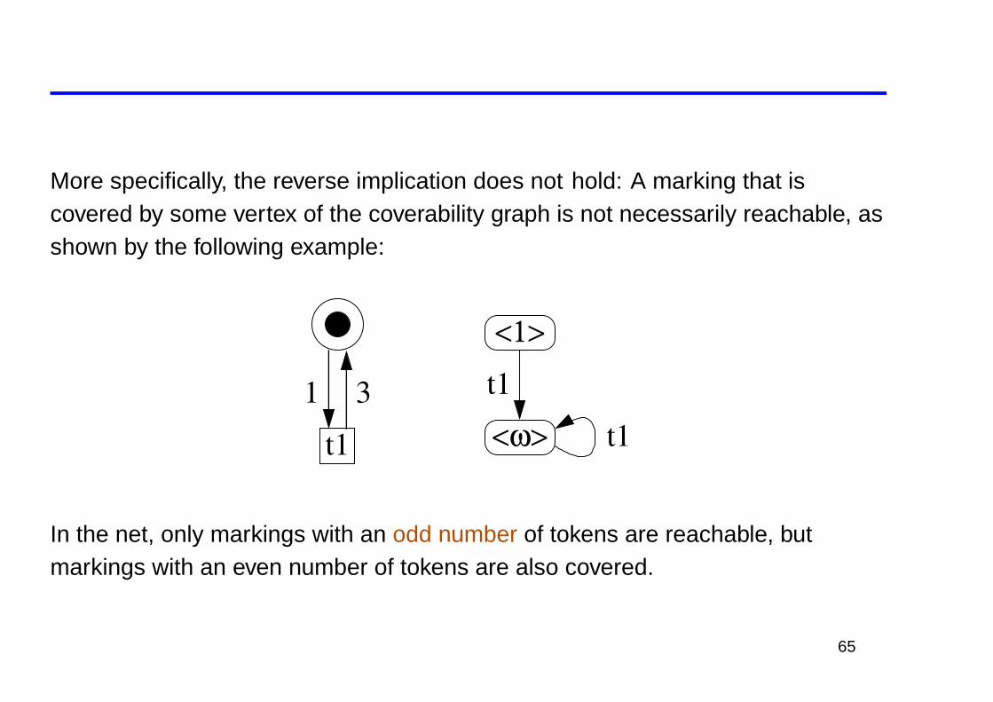
More specifically, the reverse implication does not hold: A marking that iscovered by some vertex of the coverability graph is not necessarily reachable, asshown by the following example:
t1
1 3
<1>
<ω>
t1
t1
In the net, only markings with an odd number of tokens are reachable, butmarkings with an even number of tokens are also covered.
65
Reachability and coverability graphs: Comparison (2)
The reachability graph captures exact information about the reachable markings(but its computation may not terminate).
The coverability graph computes an overapproximation(but remains exact as long as the number of markings is finite).
66
Summary: Which properties can we check so far?
Reachability: Given some marking M and a net N, is M reachable in N?More generally: Given a set of markings M, is some marking of M reachable?
Application: This is often used to check whether some ‘bad’ state can occur(classical example: violation of mutual exclusion property) if M is taken to be theset of ‘error’ states. Sometimes (as in the man/wolf/etc example), this analysiscan check for the existence of a solution to some problem.
Using the reachability graph: Exact answer is obtained.
Using the coverability graph: Approximate answer. When looking for ‘bad’ states,this analysis is safe in the sense that bad states will not be missed, but the graphmay indicate ‘spurious’ errors.
67
Summary (cont’d)
Finding paths: Given a reachable marking M, find a firing sequence that leadsfrom M0 to M.
Application: Used to supplement reachability queries. If M represents an errorstate, the firing sequence can be useful for debugging. When solving puzzles,the path represents actions leading to the solution.
Using the reachability graph: Find a path from M0 to M in the graph, obtainsequence from edge labels.
Using the coverability graph: Not so suitable – edges may represent ‘shortcuts’(unspecified repetitions of some loop).
68
Summary (cont’d)
Enabledness: Given some transition t , is there a reachable marking in which t isenabled?(Sometimes, t is called dead if the answer is no. Actually, this is a special case ofreachability.)
Application: Check whether some ‘bad’ action is possible. Also, is somedesirable action is never enabled, a ‘no’ answer is an indication of some problemwith the model.In some Petri-net tools, checking for enabledness is easier to specify thanchecking for reachability. In that case, reachability queries can be framed asenabledness queries by adding ‘artificial’ transitions that can fire iff a givenmarking is reachable.
Using the reachability graph: Check whether there is an edge labeled with t .
Using the coverability graph: ?
69
Summary (cont’d)
Deadlocks: Given a net N, is N deadlock-free?
A marking M of a Place/Transition net N = 〈P, T , F , W , M0〉 is called adeadlock if no transition t ∈ T is enabled in M. A net N is deadlock-free if noreachable marking is a deadlock
Application: Deadlocks tend to indicate errors (classical example: philosophersmay starve).
Using the reachability graph: Check whether there is a vertex without anoutgoing edge.
70
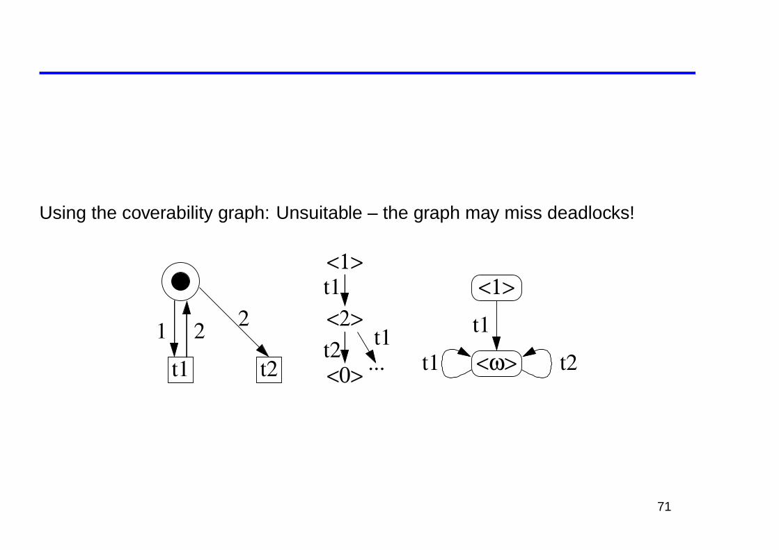
Using the coverability graph: Unsuitable – the graph may miss deadlocks!
<1>
<ω>
t1
t2t1t1
1 2
t2
2
<1>
<0>
<2>t1
t2 t1...
71
Summary (cont’d)
Boundedness: Given a net N, is there a constant k such that N is k -safe?Otherwise, which places can assume an unbounded number of tokens?
Application: If tokens represent available resources, unbounded numbers oftokens may indicate some problem (e.g. a resource leak). Also, this propertyshould be checked before computing the reachability graph!
Using the reachability graph: Unsuitable, computation may not terminate.
Using the coverability graph:
A place p can assume an unbounded number of tokens iff the coverabilitygraph contains a vertex M where M(p) = ω.Iff no vertex with an ω exists, then the net is k -safe, where k is the largestnatural number in a marking of the graph.
72
What is missing? (Outlook)
Sometimes, properties mentioned in the summary can be checked even withoutconstructing the reachability graph (which can be pretty large, after all).
Methods for doing this are collectively called structural analyses. These will becovered in the next lecture.
So far, we have not learnt how to express (and check) properties like these:
Marking M can be reached infinitely often.
Whenever transition t occurs, transition t ′ occurs later.
No marking with some property x occurs before some marking with property y has occurred.
Properties like these can be expressed using temporal logic.
73
Structural analysis of P/T nets
74
Structural analysis of P/T nets
75
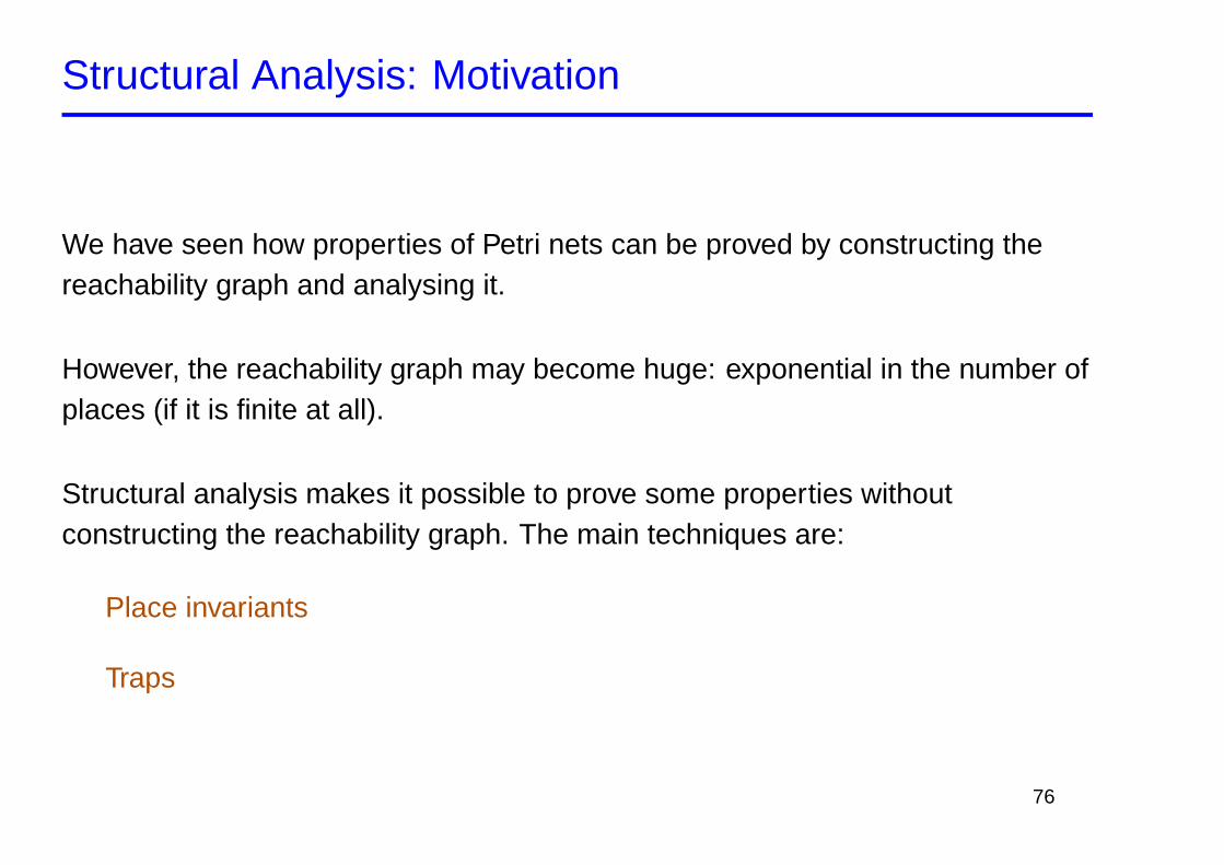
Structural Analysis: Motivation
We have seen how properties of Petri nets can be proved by constructing thereachability graph and analysing it.
However, the reachability graph may become huge: exponential in the number ofplaces (if it is finite at all).
Structural analysis makes it possible to prove some properties withoutconstructing the reachability graph. The main techniques are:
Place invariants
Traps
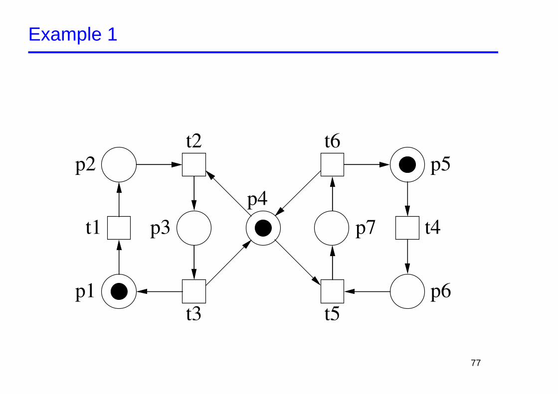
76
Example 1
p4
p5
p7
p6p1
p2
p3 t4t1
t2
t3 t5
t6
77
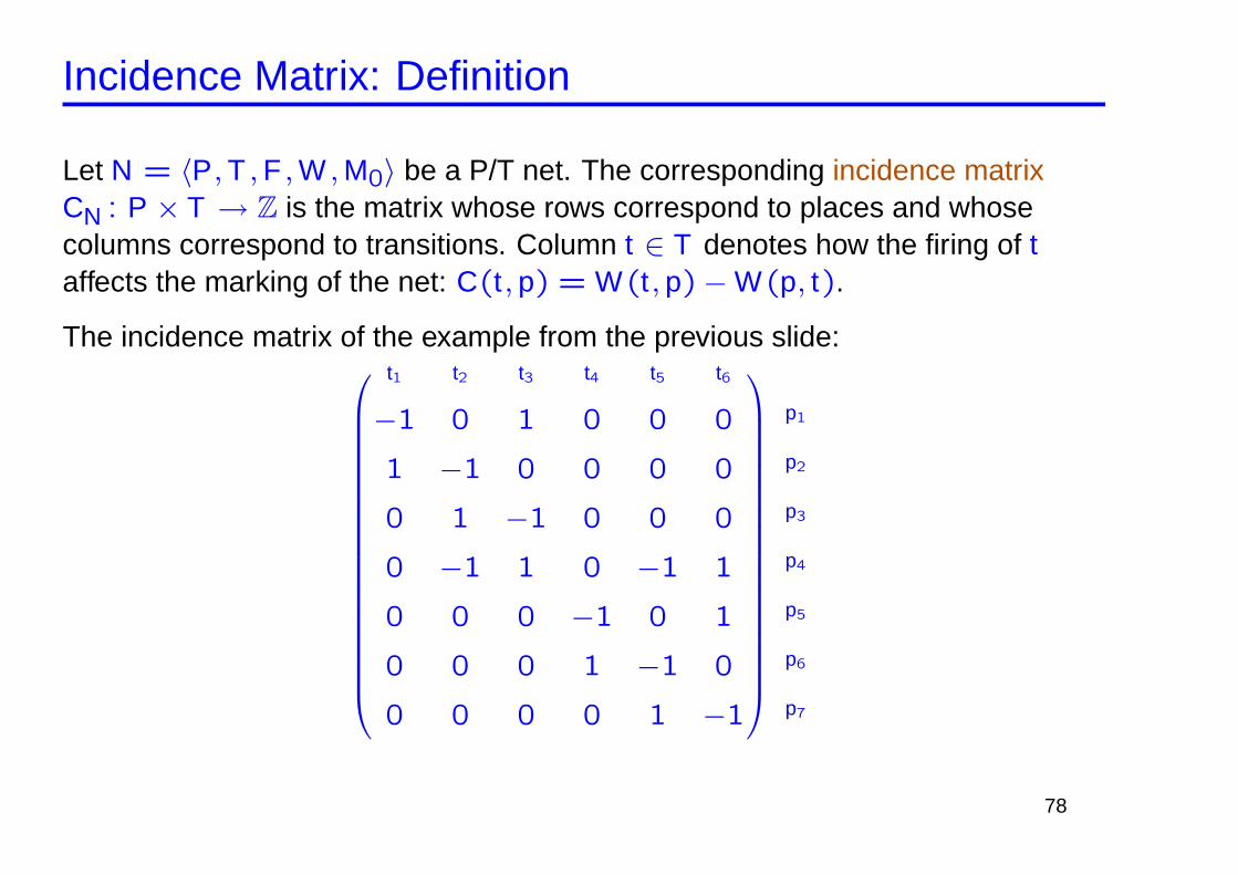
Incidence Matrix: Definition
Let N = 〈P, T , F , W , M0〉 be a P/T net. The corresponding incidence matrixCN : P × T → Z is the matrix whose rows correspond to places and whosecolumns correspond to transitions. Column t ∈ T denotes how the firing of taffects the marking of the net: C(t , p) = W(t , p)− W(p, t).
The incidence matrix of the example from the previous slide:
t1 t2 t3 t4 t5 t6
−1 0 1 0 0 0
1 −1 0 0 0 0
0 1 −1 0 0 0
0 −1 1 0 −1 1
0 0 0 −1 0 1
0 0 0 1 −1 0
0 0 0 0 1 −1
p1
p2
p3
p4
p5
p6
p7
78
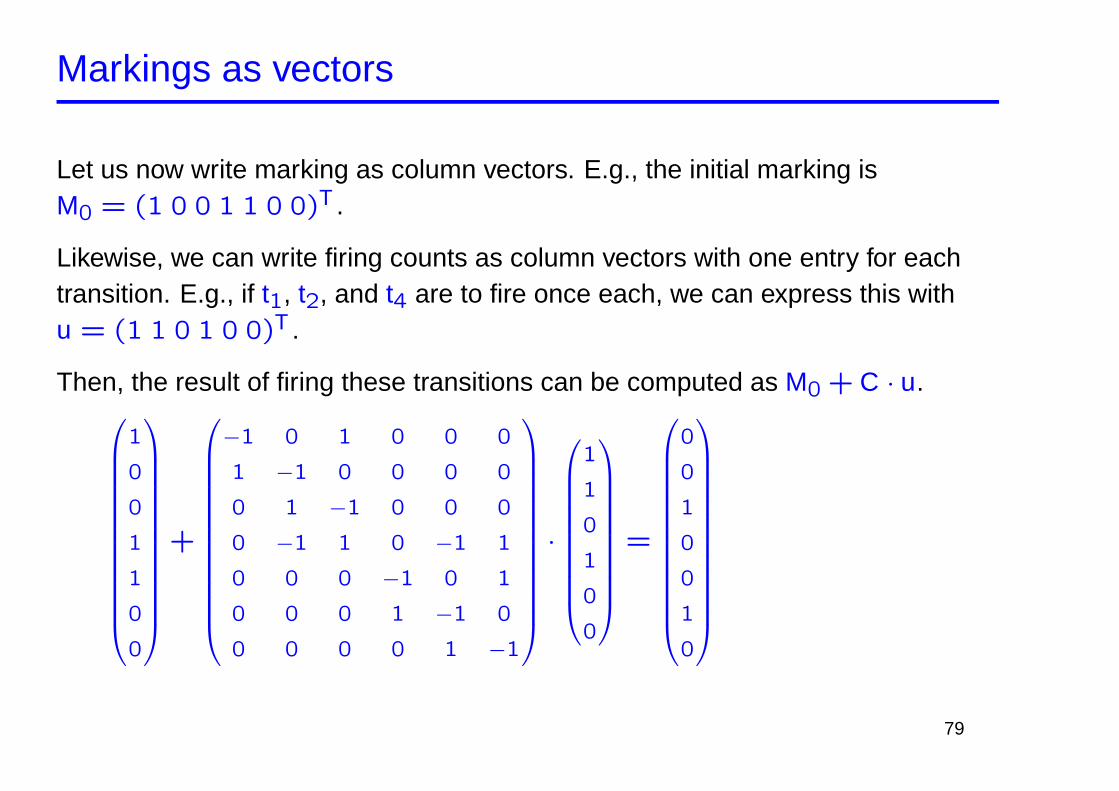
Markings as vectors
Let us now write marking as column vectors. E.g., the initial marking isM0 = (1 0 0 1 1 0 0)T .
Likewise, we can write firing counts as column vectors with one entry for eachtransition. E.g., if t1, t2, and t4 are to fire once each, we can express this withu = (1 1 0 1 0 0)T .
Then, the result of firing these transitions can be computed as M0 + C · u.
1
0
0
1
1
0
0
+
−1 0 1 0 0 0
1 −1 0 0 0 0
0 1 −1 0 0 0
0 −1 1 0 −1 1
0 0 0 −1 0 1
0 0 0 1 −1 0
0 0 0 0 1 −1
·
1
1
0
1
0
0
=
0
0
1
0
0
1
0
79
Caveat
Notice: Bi-directional arcs (an arc from a place to a transition and back) canceleach other out in the matrix!
Thus, when a marking arises as the result of a matrix equation (like on theprevious slide), this does not guarantee that the marking is reachable!
I.e., the markings obtained by the incidence markings are an over-approximationof the actual reachable markings (compare coverability graphs. . . ).
However, we can sometimes use the matrix equations to show that a marking Mis unreachable, i.e. if M0 + Cu = M has no natural solution for u.
Note: When we are talking about natural (integral) solutions of equations, wemean those whose components are natural (integral) numbers.
80
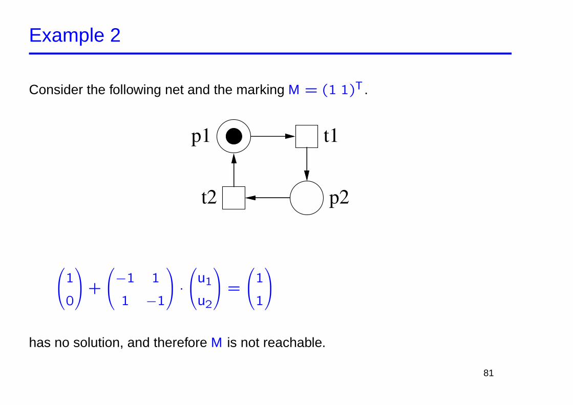
Example 2
Consider the following net and the marking M = (1 1)T .
p2
p1 t1
t2
1
0
+
−1 1
1 −1
·
u1
u2
=
1
1
has no solution, and therefore M is not reachable.
81
Invariants
The solutions of the equation Cu = 0 are called transition invariants (or:T-invariants). The natural solutions indicate (possible) loops.
For instance, in Example 2, u = (1 1)T is a T-invariant.
The solutions of the equation CT x = 0 are called place invariants (or:P-invariants). A proper P-invariant is a solution of CT x = 0 if x 6= 0.
For instance, in Example 1, x1 = (1 1 1 0 0 0 0)T , x2 = (0 0 1 1 0 0 1)T ,and x3 = (0 0 0 0 1 1 1)T are all (proper) P-invariants.
A P-invariant indicates that the number of tokens in all reachable markingssatisfies some linear invariant (see next slide).
82
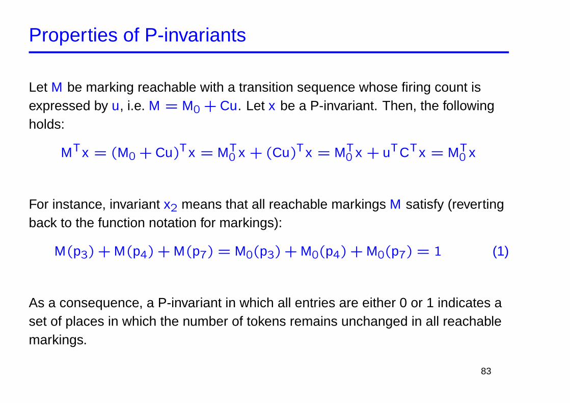
Properties of P-invariants
Let M be marking reachable with a transition sequence whose firing count isexpressed by u, i.e. M = M0 + Cu. Let x be a P-invariant. Then, the followingholds:
MT x = (M0 + Cu)T x = MT0 x + (Cu)T x = MT
0 x + uT CT x = MT0 x
For instance, invariant x2 means that all reachable markings M satisfy (revertingback to the function notation for markings):
M(p3) + M(p4) + M(p7) = M0(p3) + M0(p4) + M0(p7) = 1 (1)
As a consequence, a P-invariant in which all entries are either 0 or 1 indicates aset of places in which the number of tokens remains unchanged in all reachablemarkings.
83
Note that multiplying an invariant by a constant or component-wise addition oftwo invariants will again yield a P-invariant. That is, the set of all invariants is avector space.
We can use P-invariants to prove mutual exclusion properties:
According to equation 1, in every reachable marking of Example 1 exactlyone of the places p3, p4, and p7 is marked. In particular, p3 and p7 cannot bemarked concurrently!
Another example: Mutual exclusion with token passing (demo)
84
More remarks on P-invariants
P-invariants can also be useful as a pre-processing step for reachability analysis.
Suppose that when computing the reachability graph, the marking of a place isnormally represented with n bits of storage. E.g. the places p3, p4, and p7
together would require 3n bits.
However, as we have discovered invariant x2, we know that exactly one of thethree places is marked in each reachable marking.
Thus, we just need to store in each marking which of the three is marked, whichrequired just 2 bits.
85
Algorithms for P-invariants
A basis of the set of all invariants can be computed using linear algebra.
There is an algorithm called “Farkas Algorithm” (by J. Farkas, 1902) to computea set of so called minimal P-invariants (see the enxt slides). These are positiveplace invariants from which any other positive invariant can be computed by alinear combination.
Unfortunately there are P/T-nets with an exponential number of minimalP-invariants (in the number of places of the net). Thus the Farkas algorithmneeds (at least) exponential time in the worst case.
The INA tool of the group of Peter Starke (Humboldt University of Berlin)contains a large number of algorithms for structural analysis of P/T-nets,including invariant generation.
86
Farkas Algorithm
Input: the incidence matrix C with n rows (places), and m columns (transitions).
(C | En) denotes the augmentation of C by a n × n identity matrix (last ncolumns).
87
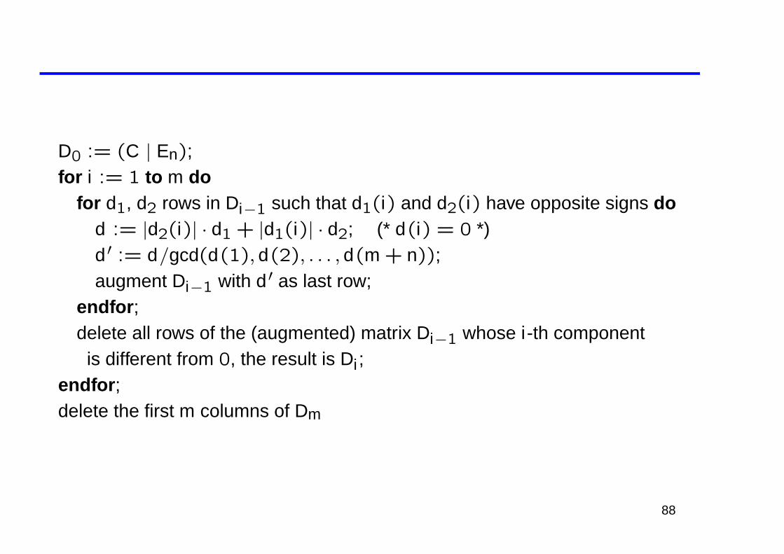
D0 := (C | En);for i := 1 to m do
for d1, d2 rows in Di−1 such that d1(i) and d2(i) have opposite signs dod := |d2(i)| · d1 + |d1(i)| · d2; (* d(i) = 0 *)d ′ := d/gcd(d(1), d(2), . . . , d(m + n));augment Di−1 with d ′ as last row;
endfor ;delete all rows of the (augmented) matrix Di−1 whose i-th component
is different from 0, the result is Di ;endfor ;delete the first m columns of Dm
88
An example
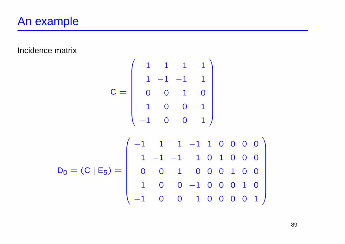
Incidence matrix
C =
−1 1 1 −1
1 −1 −1 1
0 0 1 0
1 0 0 −1
−1 0 0 1
D0 = (C | E5) =
−1 1 1 −1 1 0 0 0 0
1 −1 −1 1 0 1 0 0 0
0 0 1 0 0 0 1 0 0
1 0 0 −1 0 0 0 1 0
−1 0 0 1 0 0 0 0 1
89
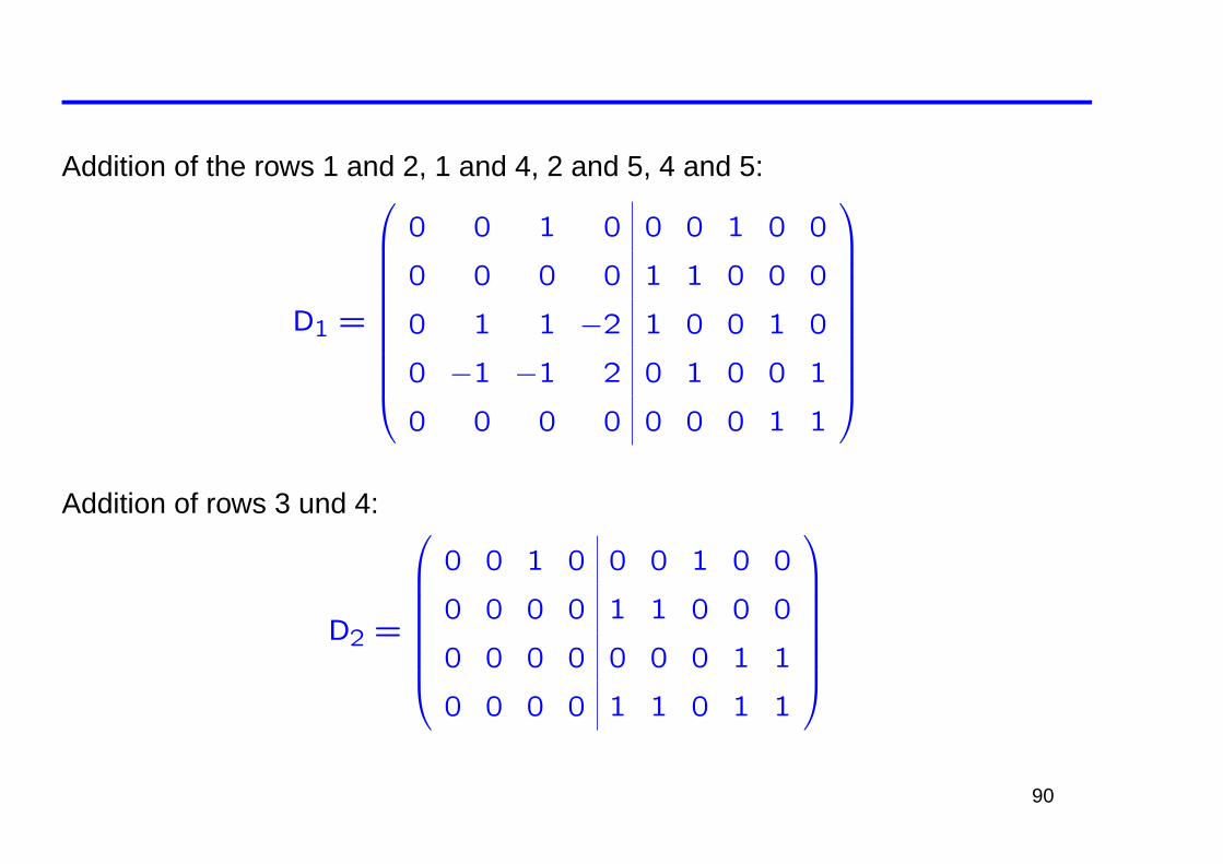
Addition of the rows 1 and 2, 1 and 4, 2 and 5, 4 and 5:
D1 =
0 0 1 0 0 0 1 0 0
0 0 0 0 1 1 0 0 0
0 1 1 −2 1 0 0 1 0
0 −1 −1 2 0 1 0 0 1
0 0 0 0 0 0 0 1 1
Addition of rows 3 und 4:
D2 =
0 0 1 0 0 0 1 0 0
0 0 0 0 1 1 0 0 0
0 0 0 0 0 0 0 1 1
0 0 0 0 1 1 0 1 1
90
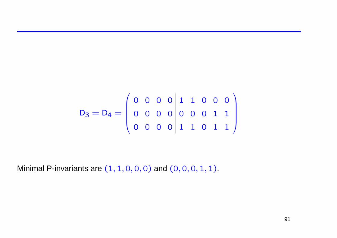
D3 = D4 =
0 0 0 0 1 1 0 0 0
0 0 0 0 0 0 0 1 1
0 0 0 0 1 1 0 1 1
Minimal P-invariants are (1,1,0,0,0) and (0,0,0,1,1).
91
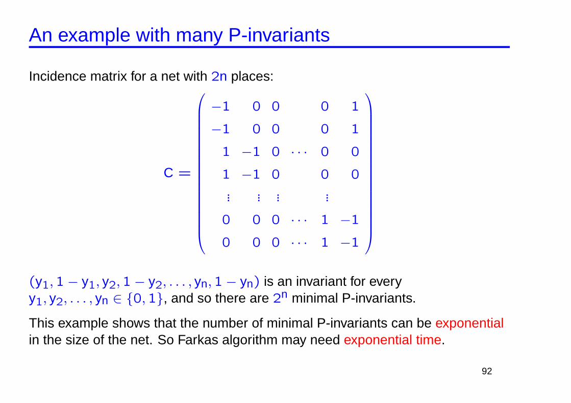
An example with many P-invariants
Incidence matrix for a net with 2n places:
C =
−1 0 0 0 1
−1 0 0 0 1
1 −1 0 · · · 0 0
1 −1 0 0 0... ... ... ...
0 0 0 · · · 1 −1
0 0 0 · · · 1 −1
(y1,1− y1, y2,1− y2, . . . , yn,1− yn) is an invariant for everyy1, y2, . . . , yn ∈ {0,1}, and so there are 2n minimal P-invariants.
This example shows that the number of minimal P-invariants can be exponentialin the size of the net. So Farkas algorithm may need exponential time.
92
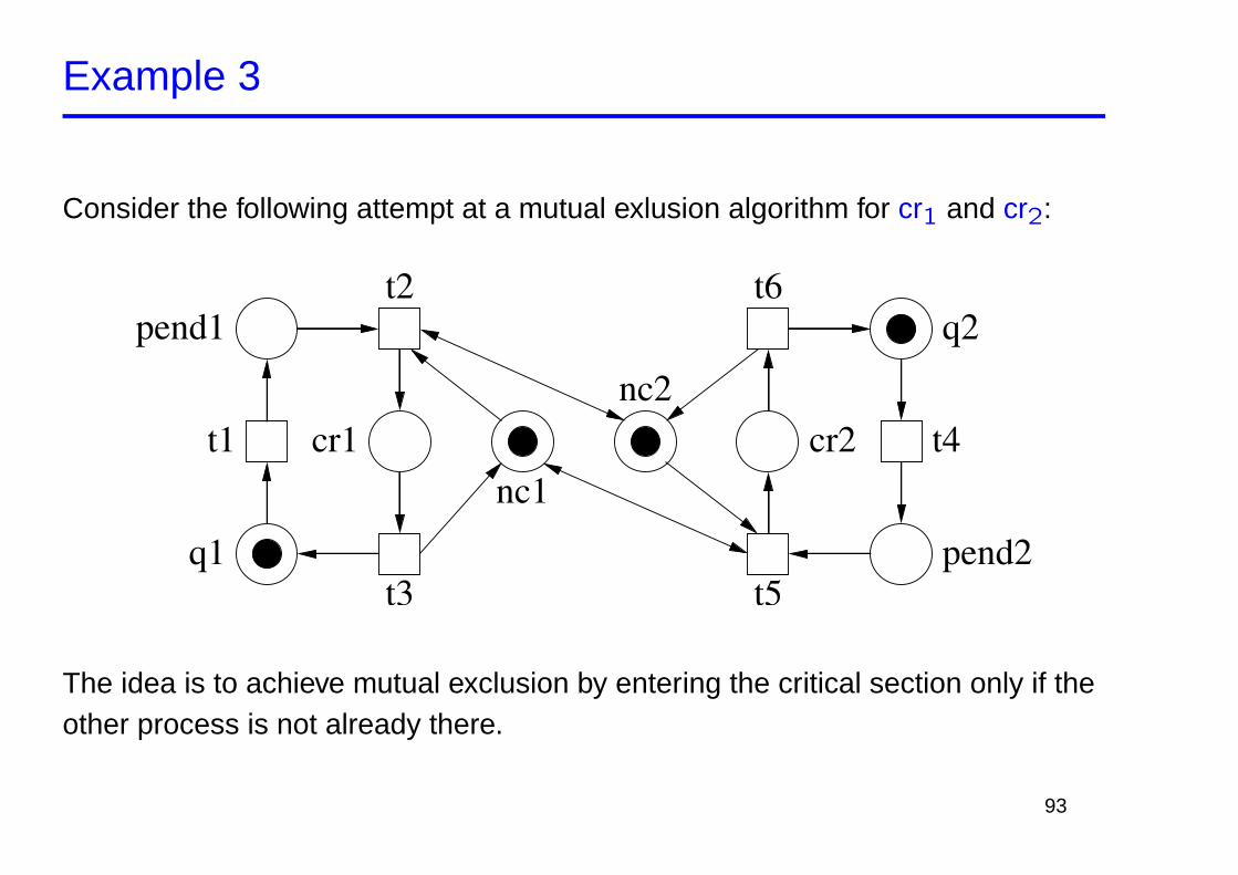
Example 3
Consider the following attempt at a mutual exlusion algorithm for cr1 and cr2:
t1
t3q1
pend1t2
cr1nc1
nc2t4
t5
t6q2
pend2
cr2
The idea is to achieve mutual exclusion by entering the critical section only if theother process is not already there.
93
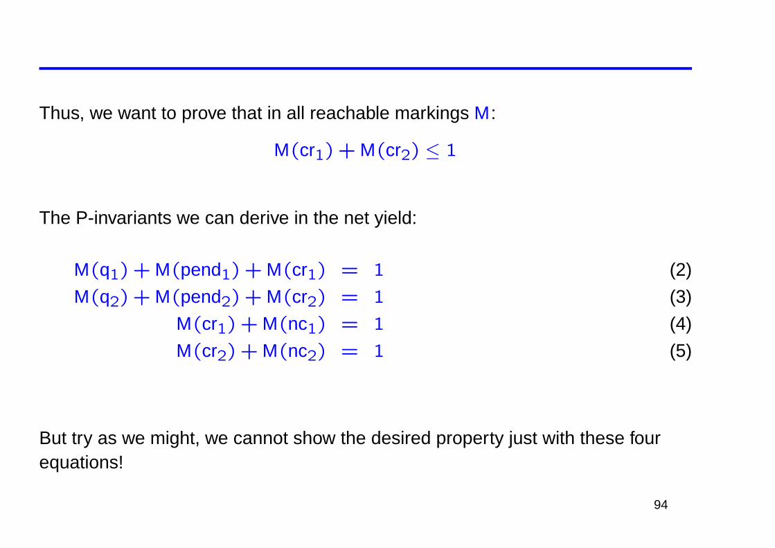
Thus, we want to prove that in all reachable markings M:
M(cr1) + M(cr2) ≤ 1
The P-invariants we can derive in the net yield:
M(q1) + M(pend1) + M(cr1) = 1 (2)
M(q2) + M(pend2) + M(cr2) = 1 (3)
M(cr1) + M(nc1) = 1 (4)
M(cr2) + M(nc2) = 1 (5)
But try as we might, we cannot show the desired property just with these fourequations!
94
Traps
Definition: Let 〈P, T , F , W , M0〉 be a P/T net.A trap is a set of places S ⊆ P such that S• ⊆ •S.
In other words, each transition which removes tokens from a trap must also putat least one token back to the trap.
A trap S is called marked in marking M iff for at least one place s ∈ S it holdsthat M(s) ≥ 1.
Note: If a trap S is marked in M0, then it is also marked in all reachable markings.
95
In Example 3, S1 = {nc1, nc2} is a trap.
The only transitions that remove tokens from this set are t2 and t5. However,both also add new tokens to S1.
S1 is marked initially and therefore in all reachable markings M. Thus:
M(nc1) + M(nc2) ≥ 1 (6)
Traps can be useful in combination with place invariants to recapture informationlost in the incidence matrix due to the cancellation of self-loop arcs.
Here: Adding (4) and (5) and subtracting (6) yields M(cr1) + M(cr2) ≤ 1, whichproves the mutual exclusion property.
96