Using a Social Experiment to Validate a Dynamic Behavioral Model of Child Schooling and Fertility:

Assessing the Impact of a School Subsidy Program in Mexico*

Petra Todd

and

Kenneth I. Wolpin

April, 2002

revised September, 2003

* We thank the National Science Foundation for support under grant #SES-0111593, the Population Studies

Center at the University of Pennsylvania for computer support and Jere Behrman for helpful comments.

Abstract

This paper studies the performance of a methodology that can be used to evaluate the impact of new policies

that radically depart from existing ones. It uses data gathered from a randomized schooling subsidy experiment

in Mexico (i) to estimate and validate a dynamic behavioral model of parental decisions about fertility and child

schooling, (ii) to forecast long-term program impacts that extend beyond the life of the experiment, and (iii) to

assess the impact of a variety of counterfactual policies. The behavioral model is estimated using data on

families in the randomized-out control group and in the treatment group prior to the experiment, both of which

did not receive any subsidy. Child wages provide a valuable source of variation in the data for identifying

subsidy effects. Using the estimated model, we predict the effects of school subsidies according to the schedule

that was implemented under the Mexican PROGRESA program. We compare the predicted impacts to the

experimental benchmarks and find that the model’s predictions track the experimental results closely. The

model is also used to simulate the effects of counterfactual programs and to find an alternative subsidy schedule

that provides greater impact on schooling achievement at similar cost to the existing program.

For a recent discussion, see Heckman (2000).1

Non-structural estimation can be used to evaluate new policies either when the policy directly varies2

itself, e.g., in the case of extrapolating the effect of say doubling the U.S. minimum wage, or when thereis policy relevant variation, e.g., extrapolating the effect of a college tuition subsidy that pays people toattend college using existing variation in tuition costs (as in Ichimura and Taber (2002)).

A nonstructural approach is not feasible in our setting as there is no policy relevant variation from which3

to extrapolate.

1

I. Introduction:

The value of empirically determining the underlying structure of economic relations in evaluating the

impact of policy interventions that radically depart from past experience is well understood (Marshak, 1953)

and, in principle, non-controversial. However, the credibility of applications of structural estimation in1

forecasting the impact of new policies is often a matter of dispute. Structural estimation requires extra-theoretic

assumptions. Within sample validation is imperfect, because pre-testing of the model’s structure on the

estimation sample is a common practice. Nonstructural estimation, when it can be used for the same purpose,

suffers from the same limitations. Parametric assumptions are required for extrapolating outside the range of

existing policy variation and specification pre-testing is also widespread. An alternative to using observational2

data to evaluate the impact of new policies is to design and implement randomized social experiments. A major

limitation of the experimental approach is that it is usually infeasible to vary treatments in a way that permits

evaluation of many different policies of interest. In this paper, we demonstrate that there is an unexploited

synergy between social experimentation and observational methods.

This paper has two goals. The first is to assess the validity of a dynamic behavioral model of parental

decision-making about fertility and children’s schooling by exploiting household data from a controlled social

experiment. The model we develop and estimate is an extension of the static quality-quantity fertility model of3

Willis(1973) and Becker and Lewis (1973) to a dynamic setting under uncertainty that combines features of

dynamic models of fertility as in Wolpin (1984) and Hotz and Miller (1993) and models of intra-household

For recent surveys of these literatures, see Behrman (1997) and Hotz, Klerman and Willis (1997).4

2

allocation of resources to children as in Becker and Tomes (1976) and Behrman, Pollak and Taubman (1986).4

The social experiment is designed to augment completed schooling levels of children in rural Mexico by

providing subsidies to parents conditional on school attendance. The validity of the model is assessed according

to how well structural estimates of the model, based on data from the randomized-out control group and from

the treatment group prior to the intervention, predict the experimental impact of the program.

The second goal of this paper is to use the structural estimates of the behavioral model to perform an

evaluation of policy interventions that are not part of the original experimental design, such as variations in the

subsidy, and to assess the longer- term impact of the program on behaviors related to child schooling decisions

that extend beyond the life of the program, such as completed family size and completed schooling of all

children ever born.

It is well known that the structural estimation of dynamic behavioral models requires auxiliary

assumptions about the functional forms of structural relationships, i.e., preferences, technology and other

constraints, and the distributions of unobservable random elements. Assessing the validity of such models by

relying on tests of model fit to sample elements of the data used in estimation provides useful, but usually not

compelling, evidence on the validity of the model. Such models are often subjected to a form of “pre-test”

estimation in that the final formulation of the model is based on the fit of prior formulations to specific

summary statistics of the data. This practice reduces the value of within-sample fit tests as a method of model

validation.

To mitigate the effect of pre-test estimation, there have been a number of attempts to assess model

validity through out-of-sample forecasts. However, such applications are sparse and have been limited by the

nature of the data. For example, Keane and Wolpin (1997) used the estimates of their model of occupational

choice, based on a cohort of young men from the NLSY79 between the ages of 16 and 26 (over the years 1978

to1988), to forecast occupational choices for the same and nearby cohorts between the ages of 27 and 44 over

Keane and Wolpin found that the structurally estimated model forecasts white-collar employment better5

than a non-structurally estimated model, but that the situation is reversed in forecasting blue-collaremployment. They also found that a model in which individuals behave myopically provided incredibleout-of-sample forecasts of occupational choices and wages.

Lumsdaine, Stock and Wise (1992) found that the structural dynamic programming model forecasts the6

impact of the window plan better than a non-structural probit specification.

In parallel work, Lise, Seitz and Smith (2003) use data from the experimental evaluation of Canada’s7

Self Sufficiency Project to test a calibrated equilibrium model of job search behavior.

PROGRESA stands for Programa de Educacion, Salud, y Alimentacion (Program of Education, Health8

and Nutrition). The name of the program was recently changed to Oportunidades, but its essentialfeatures remain the same.

3

the years 1989-1995 (using march CPS data). Although informative, because the data are highly age-trended

and the model builds in such trends, tests based on this kind of out-of-sample data may not be able to

discriminate finely among alternative models. 5

Another type of model validation test makes use of regime shifts. For example, Lumsdaine, Stock and

Wise (1992) compared the ability of structurally and non-structurally estimated models to forecast the impact of

a pension “window plan” on the departure rates of workers from a single firm. The workers were subject to a

defined benefit plan that provided a significant incentive to remain with the firm until age 55 but to leave before

65. In 1982, there was a major change in the plan and vested workers over the age of 55 were offered a bonus to

retire. Lumsdaine, Stock and Wise (1992) compare forecasts of the models’ predictions about the impact of the

bonus on retirements, based on pre-1982 data, to actual retirements. The forecast is of a large change in the

pension rules, and thus provides an arguably more convincing test of the validity of the model than do within-

sample tests. 6

In this paper, we similarly use out-of-sample forecasts to assess the validity of a structurally estimated

model, but the comparison is to a completely new program rather than a change to an existing program. We7

study the Mexican school subsidy program PROGRESA. This program was implemented as a social experiment

beginning in 1997. We obtain structural estimates of a model of household fertility and child schooling8

4

decisions using data on the randomly selected control group and on the treatment group prior to the experiment,

for whom there are longitudinal data over three survey years. We assess the performance of the model by

comparing the impact of the program predicted by the model to the impact obtained under the experiment. By

design, the control and treatment groups are randomly drawn from the same population so that the behavioral

model relevant to the control group should be the same as the model relevant to the treatment group. This

experiment therefore represents a unique opportunity to assess the validity of a structurally estimated model.

Previous studies in the program evaluation literature have also made use of social experiments to study

the performance of methods for estimating program effects using observational data. For example, Lalonde

(1986) compared estimates of the impact of a job training program based on a variety of nonexperimental

estimators to an experimental benchmark. More recently, Heckman, Ichimura and Todd (1997) studied the

performance of a class of matching estimators in a similar context. The methods studied in that literature

typically require data on program participants and are therefore not suitable for evaluating the effect of

programs that have not been implemented. In contrast, the method adopted in this paper only requires data on

nonparticipants. We show that the existence of an active child labor market and variation in child wages, a

component of the opportunity cost of school attendance, can be used to identify the parameters of our

behavioral model, which enables us to forecast the effect of a school subsidy program without any variation in

the data in the direct cost of schooling.

The model developed in this paper assumes that a married couple makes sequential decisions about the

timing and spacing of births and about the time allocation of children through age 15, including their school

attendance and labor market participation. Parents receive utility contemporaneously from the stock of children

and their current ages, their children’s current schooling levels and attendance and from their leisure time

(home production). Household consumption, which also yields contemporaneous utility, is enhanced by their

children’s earnings. The decision to bear a child (for a woman to become pregnant) is made over a finite

horizon beginning at the woman’s age at marriage and ending when the woman is no longer fecund (assumed to

5

be age 43); decisions about the time allocation of children are made through age 59. Parent’s income is an

exogenous function of the husband’s age and the distance of the village of residence to the nearest large city.

Parental preferences and income and children’s earnings are subject to time-varying stochastic shocks.

Preferences, parental income and child wages differ permanently among households according to their type,

which is unobservable to us.

Attanasio, Meghir and Santiago (2001) develop and structurally estimate a quite different model of

schooling decisions that they also use to evaluate the impact of the PROGRESA program and of variations to

the subsidy schedule. The key differences are: (i) their model assumes that schooling is chosen to maximize

each individual child’s lifetime income disregarding the intra-household allocation decision of parents, and

their model does not incorporate a fertility decision; (ii) they use data from post-program treatment households

in estimating their model; (iii) they allow the income generated by working children to have a different effect

on schooling decisions than income generated by the school subsidy, which we cannot allow for because we do

not use post-program data in the estimation; and (iv) they estimate treatment impacts allowing for the

possibility that the control group may have anticipated plans to bring them into the program at a future date.

The empirical evidence presented about the importance of anticipatory effects is mixed, with some schooling

patterns better fit by a model that assumes no anticipation, but other patterns better fit by a model with

anticipation.

Our strategy of using the treatment group to validate the model assumes that the control group did not

expect to be brought into the program. We base this assumption mainly on accounts from PROGRESA

administrative personnel that special care was taken in administering the survey so as not to inform the control

group families about the existence of the program or about future plans to incorporate them. If there were

anticipatory effects, however, we would expect them to be present in 1998 but not in 1997, because the baseline

data were gathered at a time before the initiation of the program. Thus, we would expect our model, estimated

under the assumption of no anticipation, to fit the 1997 schooling patterns better than the 1998 patterns. As

Wolpin (1996) reviews a number of examples in the context of discrete choice dynamic programming9

models.

For an alternative non-structural approach to analyzing the long-run impact of the PROGRESA10

program, see Behrman, Sengupta and Todd (2000a).

6

described later in the paper, the model fits similarly well for both years, which leads us to conclude that there is

no strong evidence of anticipatory effects.

A structurally estimated model that is a valid representation of behavior can be used to evaluate the

impact of counterfactual policies. In contrast, social experiments provide information only about the impact of9

the program as it was implemented. They cannot be used to evaluate variations in the program or longer run

effects that extend beyond the life of the experiment, and they cannot be used to evaluate radically different

programs. Using the model’s estimates, we determine the impact of the program for alternative subsidy

schedules, including halving the subsidy level, doubling the subsidy level and subsidizing attendance only in

higher grades. In addition, we evaluate two radically different programs, one that provides a bonus for

graduating from junior secondary school but no other payments and one that provides an income subsidy

without the school attendance requirement.

The model is also used to forecast long run impacts of the program, which might differ substantially

from the short-run impacts that are measured by the experiment. Even if the program was viewed by the

treatment group as permanent, the impact of the program measured by the experiment is conditioned on the

circumstances of the families at the time the program was initiated, e.g., the number of children they have and

their grade completion levels. The longer-run impact of the program may be to affect those circumstances. For

example, one long-run effect of a schooling subsidy may be to alter the number of children families have.

Another long-run impact may be to decrease the extent of discontinuous school attendance, leading to larger

long-run effects if returning to school after a period of non-attendance is viewed as costly. Evaluating the10

long-run effects of the program using an experimental approach would require that the experiment be continued

long enough to observe these changes, which is costly and often politically infeasible. We use the model to

These households account for 40 percent of all rural households and 10 percent of all households in11

Mexico (See Gomez de Leon and Parker (2000)).

Children are required to attend at least 85% of days as verified by principals and teachers.12

For example, such programs exist in Bangladesh, Pakistan, Chile, Colombia, Brazil, Guatemala, and13

Nicaragua.

7

estimate what the completed family size and completed schooling would have been for the treatment families

had the program been in existence for their entire lifetimes.

In the next section, we provide relevant details of the PROGRESA program, followed in section III by a

description of the data used in the estimation. Section IV presents the model and estimation method and section

V the results of the estimation, including an assessment of the model’s validity and of counterfactual

experiments. The latter exercise is clearly dependent on the success of the model at forecasting the impact of

the subsidy program. The model does indeed perform quite well.

II. The PROGRESA Program:

We begin with a description of the PROGRESA program and the evaluation research that has already

been performed. PROGRESA is a large-scale anti-poverty and human resource program begun in Mexico in

1997 that now provides aid to about 10 million poor families. The program was begun in rural areas and is11

currently being expanded into semi-urban and urban areas. The major goal of the program is to stimulate

investments in children’s human capital. The program attempts to align household incentives with program

goals by providing transfer payments that are contingent on children’s regular attendance at school. Programs12

with features very similar to those of PROGRESA have been initiated in many other Latin American and Asian

countries. 13

In recognition of the fact that older children are more likely to engage in family or outside work, the

transfer amount provided under the PROGRESA program varies with the child’s grade level. As seen in Table

1, it is greatest for children in junior secondary school (grades 7 through 9) and is also slightly higher for

Prior to 1992, Mexico had compulsory schooling that required that children complete at least 6 years14

of schooling. In 1992, the law was changed to require the completion of 9 years of schooling. However,as our data show, the law is not strictly enforced. Although a large proportion of children complete 6years of schooling, the vast majority complete less than 9.

Some of this aid is contingent on visiting a health clinic. 15

The 506 localities were selected in a stratified random sampling procedure from localities identified by16

PROGRESA to be eligible to participate in the program, because of a “high degree of marginality”(determined mainly on the basis of analysis of data in the 1990 and 1995 population censuses (1990Censo, 1995 Conteo)). There are 31 states in Mexico.

However, the program has recently been expanded to include many of the control localities, so that it is17

possible that the behavior of the controls groups over the time period we observe them could have beeninfluenced by their expectation of eventually receiving benefits. We present evidence about the existenceof anticipatory effects below.

8

female children, who traditionally have lower secondary school enrollment levels. In addition to the14

educational subsidies, the program also provides some monetary aid and nutritional supplements for infants and

small children that are not contingent on schooling. In total, the benefit levels that families receive are15

substantial relative to their income levels. The monthly average total cash transfer is US $55 (more than 75% is

due to the educational subsidy), which represents about one-fourth of average family income (Gomez de Leon

and Parker, 2000).

For purposes of evaluation, the second phase of the PROGRESA program was implemented as a

randomized social experiment, in which 506 rural villages (in 7 states) were randomly assigned to either

participate in the program or serve as controls. Randomization, under ideal conditions, allows mean program16

impacts to be assessed in a simple way through comparisons of outcomes for treatments and controls. Behrman

and Todd (2000b) provide evidence that is consistent with the randomization having been carefully

implemented. They document that the treatment and control groups are highly comparable prior to the initiation

of the program. Over the three year time period covered by our data, the households living in the control

villages did not receive program benefits.17

The data gathered as part of the PROGRESA experiment provide rich information at the individual and

Program eligibility is based in part on discriminant analysis applied to the October 1997 household18

survey data. The discriminant analysis uses information on household composition, household assets(such as whether the house had a dirt floor) and some other factors in determining program eligibility.

A family could participate in the health component of the program, but not in the school subsidy19

component.

9

household levels, including information on school attendance and achievement, employment and wages of

children and the income of the household. Data are available for all households located in 320 villages

randomly assigned to the treatment group and for all households located in 186 villages assigned to the control

group. The data that we analyze were gathered through two baseline surveys administered in October, 1997 and

March, 1998 and through three follow-up surveys administered October, 1998, May, 1999, and November,

1999. Households residing in treatment localities began receiving subsidy checks in the fall of 1998. In addition

to the household survey data sets, supplemental data gathered at the village level and at the school level are also

available, most importantly for our purpose, the travel distance to the nearest secondary school and to the

nearest city.

Within treatment localities, only households that satisfy program eligibility criteria receive the school

subsidies, where eligibility is determined on the basis of a marginality index designed to identify the poorest

families within each community. Because program benefits are generous relative to families’ incomes, most18

families deemed eligible for the program decide to participate in it, although not all families are induced by the

transfers to send their children to school. Data collection was exhaustive within each village and included19

children from ineligible families. There are 9,221 separate households in the control villages and 14,856 in the

treatment villages.

Most of the existing research on the PROGRESA social experiment focuses on estimating the

experimental impacts through mean comparisons of various outcome measures for treatment and control

children. Gomez de Leon and Parker (2000) and Parker and Skoufias (2000) examine how children’s time use,

e.g., time spent working for pay, differs for children participating in the program. Shultz (2000) and Behrman,

A landless household is defined as a household that reported producing no agricultural goods for20

market sale. This restriction was adopted both to make the sample more homogeneous and smaller (toreduce the computational burden) and to avoid having to model agricultural production, which would benecessary if family child labor is not a perfect substitute for hired labor. We also restricted the sample tonuclear households, which are the vast majority.

10

Sengupta, and Todd (2000a) analyze the effect of the program on school enrollment and attendance rates.

Figure 1, adapted from Behrman, Sengupta and Todd, shows the impact of the subsidy on school enrollment

rates by age and sex. Treatment impacts on enrollment rates are mainly confined to older ages, children

between the ages of 12 and 15, and are of similar magnitudes for girls and boys.

III. Variable Definitions and Descriptive Statistics:

Variable Definitions

Our estimation sample consists of landless households in which there was a woman under the age of 50

reported to be the spouse of the household head. This restriction reduced the sample to 1,531 households20

located in the control villages in 1997 and 2,162 households located in the treatment villages in 1997.

Additional exclusions based on missing or otherwise inconsistent data reduced the sample to 1,362 households

in the control villages (of which 1,355 are also observed in 1998) and 1,949 households in the treatment

villages. As of 1997, there were 4,501children born to the control households and 6,219 to the treatment

households, on average a little over 3 children per household. Of these, 2,096 children in the control village and

2,845 in the treatment villages are between the ages of 6 and 15 as of the October, 1997 survey. In contrast to

the entire sample, landless households tend to be poorer and, therefore, have a higher proportion of eligible

households. As of the 1997 survey, about 52 percent of the all households were eligible to participate in the

program, while 66 percent of the landless households were eligible to participate.

In estimating the behavioral model, we use data on both program eligible and ineligible households.

Because eligibility depends on the number of children in the family, which is a choice variable in our model,

restricting the estimation sample to eligible families would create a choice-based sampling problem of the kind

Given the specification of the model, which is described in detail in the next section, solving the21

choice-based sampling problem would require knowledge of the distribution of unobserved family typesamong both eligible and ineligible families. Using ineligible households also has the advantage ofincreasing sample variability in parental income and initial conditions.

11

that often arises in program evaluation settings. We avoid the choice-based sampling problem by using data on

both eligible and ineligible families in estimating the model. 21

Unfortunately, the PROGRESA data provide information concerning school attendance and work

essentially only at the survey dates. Therefore, allocating children to the school-work-at home categories that

pertain to an entire school year requires additional assumptions. In defining school attendance, we use the data

on school enrollment in the week prior to the survey and data on highest grade completed at the time of the

survey. Specifically, we used the following rule in determining school attendance during each of the two school

years, 1997-98 and 1998-99, covered by the surveys: (1) A child was considered as having attended school for

the entire year if a child that was reported as enrolled in at least one of the two surveys during each school year

and was reported as completing at least one grade level. (2) A child was considered as having not attended if the

child was reported as not enrolled in both surveys during each school year and did not complete a grade level.

(3) Essentially, all other problematic cases were hand-edited to provide a consistent sequence of attendance and

grade completion. A child who was determined to have attended school, but did not complete a grade level, was

assumed to have failed that school year. School attendance information was obtained for children between the

ages of 6 and 15. Highest grade completed was obtained for all children born to the woman.

A child was defined as working during the school year if the child did not attend school using the

criteria above and had been reported as working for salary (for 1997, in the October 1997 survey and for 1998,

in the October 1998 survey). The weekly wage was provided in the surveys for those who were reported

working in the week previous to the survey. A child was defined as being at home if the child was neither

attending school nor working. Parents’ weekly income was obtained from the October surveys and includes

It is extremely rare, as reported in the survey, for children to have contributed to the self-employment22

income of the household.

Weeks worked during the year were not reported in the data.23

Although mean earnings of children would appear to be large relative to parents’ income, it should be24

recognized that the figures for children represent the means of accepted wages, that is, the mean offeredwages for that relatively small fraction of children that work. Our estimates, as described below, of themean of the offered wage distribution for children is about a third of the mean of the accepted wagedistribution. Because parents’ income is mostly composed of the income of working fathers and almostall fathers work, the mean accepted and mean offered wages will be very close.

12

market earnings of both parents as well as their self-employment income. Both the children’s weekly wage22

and the parents’ weekly income were multiplied by 52 to obtain an annual equivalent. 23

Descriptive Statistics

Table 2 presents basic sample statistics. The mean age of the wives in the sample as of 1997 is 30.5,

and that of their husbands 34.4. The mean age of marriage of the women is 18.1. On average, the families had 3

children as of 1997 and added another .2 children by 1998.The mean highest grade completed of children age 7

to 11 is 2.4 years of schooling, while children who were between the ages of 12 and 15 had completed 5.8

years, and those age 16 and over, 6.6 years. As also shown, there is almost no difference in the completed

schooling of this latter group by sex. Parent’s income over the two survey years was, on average, about 12,000

pesos (approximately 1,100 U.S. dollars). Approximately 8 percent of children between the ages of 12 and 15

were working over the two years. Among those that worked, their average income ranged from about 6,000

pesos for those 12 and 13 years of age to about 9,000 pesos for those who were 15 years of age. 24

Data were also collected about the households’ villages. Two “distance” variables are of particular

relevance: the distance from the village to a junior secondary school and the distance from the village to the

nearest city. As seen in Table 2, about one-quarter of the villages have a junior secondary school located in the

village, and among those villages that do not, the average distance to a village with a secondary school is

We thank T. Paul Schultz for making this data available to us. 25

Child labor laws prohibit children under the age of 14 from working and also limit the kinds of26

employment and the length of the work day. Our model assumes that these restrictions are not binding,which is consistent with the fact that we observe children under the age of 14 who are working. A verysmall number of children were working before the age of 12. We assumed that, in fact, they were at homein order to avoid having to fit the model to those few observations.

13

approximately three kilometers. The villages are also generally quite distant from major cities. The average

distance of the households from a city is 135 kilometers. 25

Table 3 provides more detail concerning the time allocation of children. The first two columns contrast

the reported school attendance rates (in percent) of children by sex from ages 6 through 15 based on the raw

data, whether or not the child was enrolled as of the October 1997 interview date (in column one), and the

revised rates based on the rules described above (in column 2). The third column shows the percentage of

children working for pay and the last column the percentage at home (100 - (2) - (3)).

As is apparent from comparing the first two columns, the revised attendance rates are slightly higher

than the raw attendance rates. Based on the revised rates, school attendance is almost universal from ages 7 to

11 for both boys and girls. Attendance at age 6 is lower, particularly for boys, although over 90 percent.

Attendance rates fall to 89 percent for males and to 90 percent for females at age 12, an age by which many

children have completed primary school (grade 6). After age 12, attendance rates continue to decline for both

girls and boys, but more rapidly for girls. By age 15, attendance rates are only 48 percent for boys and 40

percent for girls. The percentage of children working for pay at age 12 is only 2.5 for boys and 1.1 for girls. By

age 15, 28 percent of boys but only 16 percent of girls are working for pay.26

Girls progress through the early grades somewhat faster than boys, but ultimately complete about the

same amount of schooling. As of October 1997, girls who are 12 years of age have completed about .3 more

years of schooling on average than have boys of the same age. At age 16, that difference has completely

disappeared, with both sexes having completed, on average, 6.6 years of schooling. Girls are more likely to

complete sixth grade, but are also more likely drop out of school after completing it. As seen in Table 4, among

National examinations are given at each primary grade level and adequate performance determines27

grade progression, although compliance is left to teachers. Certificates are awarded after the completionof primary school and junior secondary school.

The duration to the first birth is calculated as the age of the woman in 1997 minus the age of the child28

in 1997 minus the age of the woman at marriage. Ten percent of first births were reported to haveoccurred at an age prior to the woman’s age at marriage and 14 percent coincident with the woman’s ageat marriage. For the cases where the birth occurred at or before the age at marriage, the marriage wasassumed to have occurred one year prior to the birth of the first child. An additional 26 percent of firstbirths occurred at an age one year post-marriage. The sum of these is about equal to the 52 percent offirst births occurring in the first year of marriage reported in the table.

14

the children in our sample who are age 15 or 16 in 1997, 22 percent of the boys and 17 percent of the girls have

less than 6 years of schooling, 32 percent of the boys and 39 percent of the girls have exactly 6 years of

schooling and 46 percent of the boys and 44 percent of the girls have more than 6 years of schooling. Failure

rates are slightly higher for boys than for girls, 15.2 percent for boys and 14.5 percent for girls over all grades,

but considerably higher at the primary grades, 15.7 percent vs. 13.9 percent.27

Table 5 provides information about fertility patterns. In particular, it shows the duration distribution

from the date of marriage to the birth of each of the first three children. Fertility occurs rapidly after marriage.

A little more than 50 percent of the women had their first birth within a year of marriage. First births occurred28

within two years for seventy percent of the women. As the second column shows, of the women who had at

least two children, only 11 percent of the women had two births in two years, but 35 percent had their second

birth within 3 years of marriage and two-thirds within 5 years. About 10 percent did not have their second birth

until after 10 years of marriage. Over 20 percent of the women who have at least three children had their third

birth after 10 years of marriage. Thus, most women have their births quickly after marriage, although some

delay for a significant period.

Once children leave school, they rarely return. As seen in Table 6, only 13 percent of boys age 13 to 15

who worked in one year attended school in the next year. Similarly of those who were home in one year, only

15 percent attended school in the next year. Comparable figures for girls are 20 percent (although the sample

size is only 5) and zero percent. The school-to-school transition over these ages exhibits substantial permanence

)

)

)2

w )

1F((wi)/))

)

More precisely, in order to use the probability statement above to estimate the parameters, we need to29

observe child wage offers. If we observe only accepted wages, that is, the wages of children who work,then we need to able also to identify the parameters of the offered wage distribution together with and . Standard arguments for selection models hold for the identification of the wage offer parameters,namely functional form and distributional assumptions. Identification of and requires an exclusionrestriction, a variable that affects the offered wage but not the family’s preference for child schooling.Below, we discuss the specific identifying assumptions in the richer model that we estimate.

15

for both boys and girls, with 86.2 percent of the boys and 76.9 percent of the girls who attended school in one

year also attending in the next year. The home-to- home transition for girls and the work-to-work transition for

boys also exhibit such permanence. Among girls in this age group 92.5 percent of those who were home in one

year were also home in the next year, and among boys 62.5 percent of those who worked in one year were also

working the next year.

IV. The Model:

An Illustrative Model and Identification of Subsidy Effects

Given that there is no direct cost of schooling through junior secondary school, and thus no variation

from which to directly estimate the impact of a subsidy to attendance, it is useful to consider an illustrative

model to demonstrate what information in the data would enable one to forecast the impact of the subsidy

program. Consider, then, a household with one child making a single period (myopic) decision about whether to

send the child to school or to work, the only two alternatives. Let utility of the household be separable in

consumption (C) and school attendance (s), namely u = C + ( )s, where s=1 if the child attends school and

0 otherwise and is a preference shock. Assume that the preference shock is normally distributed with mean

zero and variance . The family’s income is y + w(1-s), where y is the parent’s income and w is the child’s

earnings if working. Under utility maximization, the family chooses to have the child attend school if and only

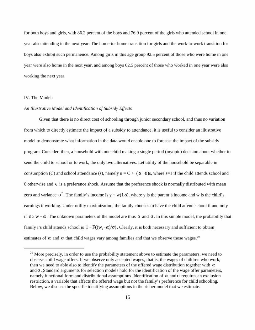
if . The unknown parameters of the model are thus and . In this simple model, the probability that

family i’s child attends school is . Clearly, it is both necessary and sufficient to obtain

estimates of and that child wages vary among families and that we observe those wages.29

F((wb)/))F((w) /))

)

tm

See Wolpin (1999) for a similar analysis of the informational content of probabilistic subjective30

expectations.

Although some information on contraceptive use is available, it is not detailed enough to allow31

modeling contraceptive decisions.

Labor force participation rates of married women in this sample are quite low, between 10-20% at32

most ages.

16

Now, suppose the government is contemplating a program to increase school attendance of children

through the introduction of a subsidy to parents of amount b if they send their child to school. Under such a

program, the probability that a child attends school will increase by . As this

expression indicates, knowledge of and is sufficient to forecast the impact of the program. Moreover, it30

is also sufficient to enable forecasts of the effect of varying the amount of the subsidy on school attendance.

Variation in the opportunity cost of attending school, the child market wage, thus serves as a substitute for

direct variation in the monetary (tuition) cost of schooling.

Model Description

In each discrete time period, a married couple makes fertility and child time allocation decisions.

Specifically, a decision is made about whether or not to have the woman become pregnant, and have a child in

the next period, and, for each child between the ages of 6 and 15, whether or not to send the child to school,

have the child work in the labor market (after reaching age 12) or have the child remain at home. At ages older31

than 15, children are assumed to become independent, making their own schooling and work decisions. A

woman can become pregnant beginning with marriage (at age t = ) and ending at some exogenous age (at t =

T-1) when she becomes infecund. The contribution of the husband and wife to household income is exogenous

(there are no parental labor supply decisions) and stochastic, and the household cannot save or borrow. The32

contributions to household income from working children (under the age of 16) are pooled with parental income

in determining household consumption.

-

- - -n

- -

It is more straightforward to treat these costs as utility losses rather than monetary costs. Given that33

monetary costs associated with school attendance are not observed in the data, consumption and psychiccosts are indistinguishable.

Bold type is used to indicate a vector.34

17

Children who neither attend school nor work for pay are assumed to contribute to household production

and thus to parental utility. Therefore, the cost of sending a child to school consists of the opportunity loss in

either home production or household income, each of which may differ by the child’s age and sex. Parents are

also assumed to derive utility in each period from the current average level of schooling that their children have

completed, from the current number of children who have graduated from elementary school (grade 6) and from

the current number who have graduated from junior secondary school (grade 9). Schooling is publicly provided

and therefore parents bear no direct tuition costs. All of the villages have their own primary schools (grades 1

through 6), but not all villages have junior secondary schools (grades 7 through 9). We allow for a psychic cost

of attending a junior secondary school that varies with the distance to the nearest village with a secondary

school, for a potential utility loss from interrupted schooling, that is, sending children to school who are behind

for their age and for an additional loss if a child attends grade 10, which often involves living away from

home.33

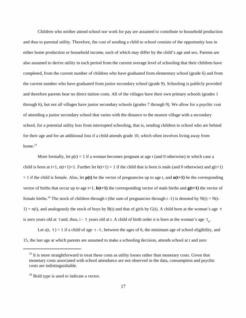
More formally, let p(t) = 1 if a woman becomes pregnant at age t (and 0 otherwise) in which case a

child is born at t+1, n(t+1)=1. Further let b(t+1) = 1 if the child that is born is male (and 0 otherwise) and g(t+1)

= 1 if the child is female. Also, let p(t) be the vector of pregnancies up to age t, and n(t+1) be the corresponding

vector of births that occur up to age t+1, b(t+1) the corresponding vector of male births and g(t+1) the vector of

female births. The stock of children through t (the sum of pregnancies through t -1) is denoted by N(t) = N(t-34

1) + n(t), and analogously the stock of boys by B(t) and that of girls by G(t). A child born at the woman’s age

is zero years old at and, thus, t - years old at t. A child of birth order n is born at the woman’s age .

Let s(t, ) = 1 if a child of age t - , between the ages of 6, the minimum age of school eligibility, and

15, the last age at which parents are assumed to make a schooling decision, attends school at t and zero

- - - - - -

%c(t1,-,S(t1) |s(t1)1,µc) µc

S(t)

S(t)

- -

- -

-

- -

(1)U(t) U(C(t), p(t), n(t), lb(t), lg(t), sb(t), sg(t), S(t);

zs, p(t), lb(t), lg(t); µN, µS, µlg , µlb ) ,

zs

µ

18

otherwise. The corresponding vector of school attendance decisions for school age children at t is s(t), where

an element is zero when there does not exist a child of a given age. Cumulative schooling at t for a child born at

is given by S(t, ) = S(t-1, ) + c(t-1, ) s(t-1, ), where c(t-1, ) =1 if a year of schooling is successfully

completed and zero otherwise. The completion of a grade level conditional on attendance is probabilistic. The

probability of completion is given by , where is a permanent family-

specific component of the success probability. The completion probability also may differ by the child’s sex.

The vector of cumulative schooling at t over all children is and the mean schooling level of those children

at t, . Sex-specific schooling variables are similarly defined and denoted with b or g subscripts.

Finally, let h(t, ) = 1 if a child born at works at t, and zero otherwise, with h(t) the corresponding

vector over all children at t. Children must be at least twelve years old to be eligible for work, i.e., h( +k, )=0

for k<12. A child who is neither in school nor at work is by definition at home, which we denote as l(t, ) =1 -

h(t, ) - s(t, ). Sex-specific variables, as before, carry b and g subscripts.

The utility function is given by

where C(t) is household consumption, is the distance to a secondary school, the ‘s are stochastic shocks to

being pregnant and to the value attached to having children of each sex at home and the ‘s reflect permanent

differences across households in their preferences for children, for schooling and for the home time of children

by sex. The parental utility function (1) is written generally enough to include the possibility, for example, that

the value of household production is greater for older girls when there are also very young children in the

yp yo

(2) C(t) yp(t) (n

yo(t, -n)h(t, -n) .

ap(t)

zc yp(t)

µyp

yo(t)

µyo

(3)

yp(t) yp(ap(t), zc, yp(t); µyp

)

yo(t, -n) yo(t-n, I(b(-n) 1), zc, yo(t); µyo

) .

It is the absence of economic theory about the form of the utility function and our inability to directly35

elicit preferences that makes necessary pre-testing of the model.

Child rearing costs are essentially indistinguishable from the psychic value of children of different36

ages, which is included in parental utility rather than in the budget constraint.

Parental education does not directly affect income, but instead enters the parent income function37

through its relationship to the unobservable parental type.

19

household. The exact representation of the utility function, which is shown in Appendix A, was determined in

part using model fit criteria. 35

Family consumption at t is equal to total family income. Family income is the sum of parental income

( ) and the earnings of children ( ) who work in the market. Thus, the family’s budget constraint is given36

by

Income generating functions differ for parents and children. Parental income at t, which includes both

earnings and self-employment income, depends on the age of the male parent ( ) , on the distance of the

household’s village from a city ( ), a random shock at t ( ) and a permanent parent-specific unobservable

component ( ). Similarly, the earnings of a child depends on the child’s age and sex, on the distance of the37

household’s village from a city, on a time-varying (but not child-varying) shock ( ) and on a permanent

unobservable component ( ) that is the same for all children (within the same household). The distance from

a city affects wage offers due to differences in the skill price reflecting the extent of the labor market to which

the household has access. Specifically,

f((t))

g(µ)

dk(t)1

6(t)

b(t) g(t) Sb(t) Sg(t) ap(t) (t) µ tm zs zc

(4) V(6(t), t) maxkK(t)

E(T

-t -tU(t) 6(t)!

T

The implicit time-varying shock to grade completion is assumed to be independent of all other shocks38

in the model.

The integration is also performed over whether a birth outcome is a boy or a girl. We assume the39

probability of each gender outcome to be .5.

20

The five time-varying -shocks are assumed to be jointly serially uncorrelated. Their joint

contemporaneous distribution is denoted by . The permanent components of parental preferences and38

income, of child earnings and grade completion are also assumed to be jointly distributed according to . In the

application, we assume g to be discrete with a fixed number of support points, which we denote as indicating

family “type.” These permanent components are known to parents from the beginning of the marriage.

At any t, the couple is assumed to maximize the present discounted value of remaining lifetime utility. In

any period, the family will face K(t) mutually exclusive alternatives, where K varies over time with the number of

children eligible to attend school and work and the woman’s age. Define if the kth alternative is chosen at

t, and = 0 otherwise. (The ordering of the K(t) alternatives is irrelevant.) Further, define to be the state space

at t, namely all of the relevant factors that affect current or future utility or that affect the distributions of future

shocks, that is, , , , , , , , , , .

The maximized present discounted value of lifetime utility at t, the value function, is given by

where is the end of the couple’s life (woman’s age 59) and the expectation is taken over the distribution of

parental preference and income shocks, the children’s earnings shock and the implicit shocks to grade completion

for choices that involve school attendance. The solution to the optimization problem is a set of decision rules that39

relate the optimal choice at any t, from among the feasible set of alternatives, to the elements of the state space at t.

Recasting the problem in a dynamic programming framework, the value function can be written as the maximum

(5)

V(6(t), t) maxkK(t)

[V k(6(t), t)]

V k(6(t), t) U k(t, 6(t)) E(V(6(t1), t1|dk(t)1),6(t)) for t < T,

U k(T, 6(T)) for t T.

V k(6(t), t) kK(t)

EV(6(t1), t1 dk(t)1,6(t)) 6(t)

Emax

2#3N1(t)

N1(t)

Violations of the assumption in the 1997 survey occur in about 5% of the households in the case of40

schooling and in about 1% of the households for working.

21

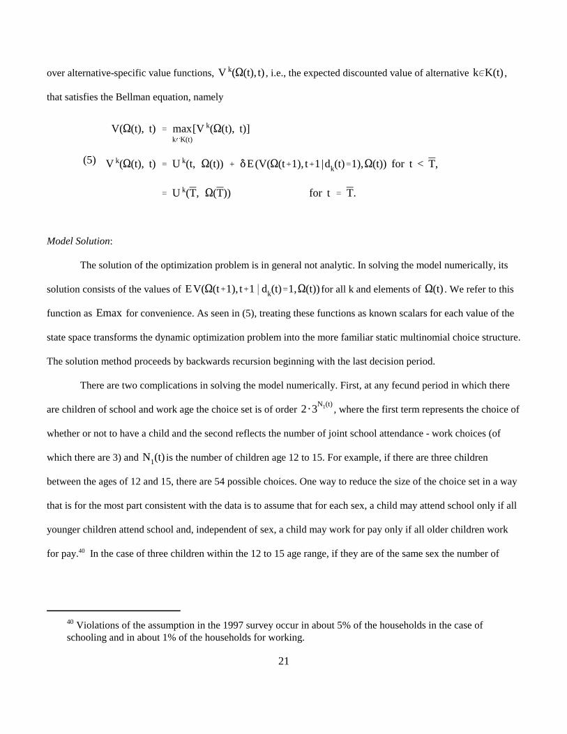
over alternative-specific value functions, , i.e., the expected discounted value of alternative ,

that satisfies the Bellman equation, namely

Model Solution:

The solution of the optimization problem is in general not analytic. In solving the model numerically, its

solution consists of the values of for all k and elements of . We refer to this

function as for convenience. As seen in (5), treating these functions as known scalars for each value of the

state space transforms the dynamic optimization problem into the more familiar static multinomial choice structure.

The solution method proceeds by backwards recursion beginning with the last decision period.

There are two complications in solving the model numerically. First, at any fecund period in which there

are children of school and work age the choice set is of order , where the first term represents the choice of

whether or not to have a child and the second reflects the number of joint school attendance - work choices (of

which there are 3) and is the number of children age 12 to 15. For example, if there are three children

between the ages of 12 and 15, there are 54 possible choices. One way to reduce the size of the choice set in a way

that is for the most part consistent with the data is to assume that for each sex, a child may attend school only if all

younger children attend school and, independent of sex, a child may work for pay only if all older children work

for pay. In the case of three children within the 12 to 15 age range, if they are of the same sex the number of40

330

Stinebrickner (2001) develops a local approximation to the Emax function.41

Only about 3 percent of women in our sample report having more that eight children. In the empirical42

implementation, we assume that children of birth order greater than eight were not born.

We used 2500 state points for the estimation of the Emax approximations and 50 draws for the43

numerical integrations. The Emax approximations did not appear to be sensitive to increases in theseparameters, up to 10,000 state points and 300 draws. There were approximately 150 variables used in theEmax approximation, which includes interactions among the state variables. The R-squares were above.99 in all time periods.

22

alternatives is now reduced to 20. We do not impose these restrictions on 6 and 7 year old children to

accommodate the fact that school entry is sometimes delayed.

Second, the size of the state space makes a full solution of the problem computationally intractable. The

Emax functions must be calculated for all state values at each t. As long as the ages of children affect lifetime

utility, as it must because of the age restrictions on children’s eligibility for schooling and work, the state space

will include the entire sequence of births by sex and not simply the stock of children. With 30 fecund periods, there

are such sequences. In addition at any t, the schooling level of each child affects expected lifetime utility at t.

To solve the dimensionality problem, we adopt an approximation method in which the Emax functions are

expressed as a parametric function of the state variables or composites of the state variables using methods

developed in Keane and Wolpin (1994, 1997, 1999). In particular, the Emax functions are calculated at a subset of

the state points and their values are used to fit a global polynomial approximation in the state variables. To41

further limit the size of the state space, we also assume that women can have no more than eight children. As in42

Keane and Wolpin, the multivariate integrations necessary to calculate the expected value of the maximum of the

alternative-specific value functions at those state points are performed by Monte Carlo integration over the -

shocks.43

Model Estimation:

The solution to the agents’ maximization problem serves as input into estimating the parameters of the

model. The numerical solution method described above provides (regression approximations to) the Emax

O(t)dk(t),yo(t),c(t),yp(t)!

tmn tn

(6) $N

n1Pr(O(tn), ...... , O(tm1,n), O(tmn)) 6(tmn),µ),

6(tmn)

µ tmn

tmn tmn

(7) $N

n1M

J

j1Pr(O(tn), ...... , O(tm1,n), O(tmn)) 6(tmn), typej)Pr(typej 6(tmn)) ,

23

functions that appear on the right hand side of (5). The alternative-specific value functions, V (t) for k=1,..,K(t),k

are known up to the parental random preference and income shocks and the earnings shock of the children. Thus,

conditional on the deterministic part of the state space, the probability that an agent is observed to choose option k

takes the form of an integral over the region of a subset of the random shocks such that k is the preferred option.

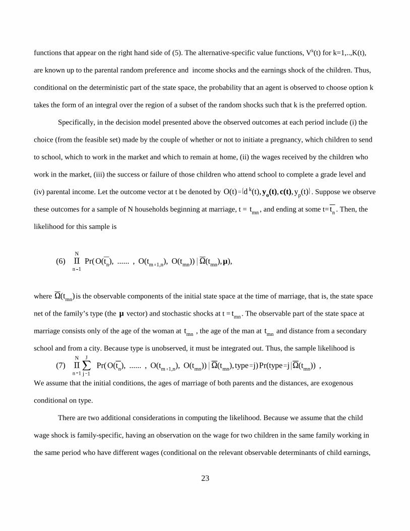
Specifically, in the decision model presented above the observed outcomes at each period include (i) the

choice (from the feasible set) made by the couple of whether or not to initiate a pregnancy, which children to send

to school, which to work in the market and which to remain at home, (ii) the wages received by the children who

work in the market, (iii) the success or failure of those children who attend school to complete a grade level and

(iv) parental income. Let the outcome vector at t be denoted by . Suppose we observe

these outcomes for a sample of N households beginning at marriage, t = , and ending at some t= . Then, the

likelihood for this sample is

where is the observable components of the initial state space at the time of marriage, that is, the state space

net of the family’s type (the vector) and stochastic shocks at t = . The observable part of the state space at

marriage consists only of the age of the woman at , the age of the man at and distance from a secondary

school and from a city. Because type is unobserved, it must be integrated out. Thus, the sample likelihood is

We assume that the initial conditions, the ages of marriage of both parents and the distances, are exogenous

conditional on type.

There are two additional considerations in computing the likelihood. Because we assume that the child

wage shock is family-specific, having an observation on the wage for two children in the same family working in

the same period who have different wages (conditional on the relevant observable determinants of child earnings,

y obso (t)yo(t)exp((t))

tm

We follow this strategy as opposed to allowing for child-specific wage shocks to avoid having to44

integrate over all of the child shocks in calculating the Emax functions. The problem of degeneracy existsmore generally, namely that with family level shocks some choices may not be generated by the model.Restricting the choice set as above reduces the likelihood of this event, but does not eliminate itnecessarily. Estimation is feasible when such events occur because our procedure smooths over zerolikelihood events (see below). After estimating the model, we verified that simulations of the modelcould generate all of the outcomes that were observed in the data, so none of these outcomes has zeroprobability of occurrence.

24

child age and sex as in (3)) will lead to a degenerate likelihood. We therefore assume that the children’s wages are

measured with error, which seems like a reasonable assumption in any event. Thus, assuming a multiplicative44

measurement error, observed child earnings is given by .

Another difficulty arises because, for most of the families, we do not observe decisions from the start of

marriage. In particular, although we have a complete fertility history for all women, we do not have a complete

school attendance and work history for children who are above the school or work eligibility ages at the first

survey. For example, consider a family with 3 children whose ages are 10, 13 and 16 as of the October 1997 survey

date and whose marriage occurred in 1980 when the woman was age 19 ( ). For this family, we observe fertility

outcomes at every t between 1980 and 1997, the woman’s age 19 through 36. However, we are missing the

complete history of school decisions for all children above the age of 6, and the work decisions for all children

above the age of 12, as of 1997. Although it is conceptually straightforward to accommodate this feature of the

data into the likelihood function (7), it is computationally infeasible to perform the integrations over all of the

feasible unobserved choice paths as would be required to calculate the likelihood.

To avoid having to deal with missing data on the schooling and work decisions of children, one could

restrict the sample to marriages that occurred between 1989 and 1997 for whom there are complete data. But for

the earliest marriages in this range, the oldest age a child could be in 1997 is 6, the first age at which a schooling

decision is made. It is obviously not possible to identify all of the parameters of the model solely from those

observations, because children do not start work for pay until age 12.

(8) $N

n1M

J

j1Pr(O(t98

n ), O(t97n ) 6(t 97

n ), typej)Pr(typej 6(t 97n )) ,

t 97n t 98

n

(t)

This is exactly the initial conditions problem in discrete choice models as discussed in Heckman45

(1981).

25

For all families, we observe the complete set of outcomes in the two survey years, 1997 and 1998. The

difficulty in using that data is that the state variables at the time of the surveys, including for instance the birth

history and the schooling levels of all children, are not exogenous. The assumption of serial independence in the45

shocks, however, implies that the state variables at any time t are exogenous with respect to decisions at t

conditional on type. Thus, the likelihood for the observations in 1997 and 1998 can be written, analogous to (7),

where and are the ages of the woman in 1997 and 1998. A problem with (8) is that we must specify how

the type distribution is related to the state variables. In actuality, the form of this conditional distribution function

is given by the structure of the behavioral model together with the relationship between type and the initial state

variables, i.e., the second term in (7). There is clearly a trade-off in how one specifies this conditional type

distribution. The more flexible the functional form the better the approximation to its true functional form and the

closer the exogeneity requirement is met. However, the more flexible the form, the more parameters there are to

estimate. Furthermore, these parameters are themselves functions of the structural parameters; the estimation

method is thus not efficient.

To summarize, in estimating the model we use (7) for the families with complete decision histories as

described above (Sample A) and we use (8) for the families with incomplete decision histories (Sample B),

ignoring the information about pregnancy decisions made prior to 1997 . Now, given the assumption of joint serial

independence of the vector of shocks (conditional on type), both (7) and (8) can be written as the product of

within-period outcome probabilities conditional on the corresponding state space and type. Each of these

conditional probabilities are of dimension equal to the number of contemporaneous shocks in .

p(t),lb(t),lg(t),yp(t),(t) yo

(t)

exp[Vk(t)max(V j(t))

-]/M

i

exp[Vi(t)max(V j(t))

-]

dk(t) -

yoj(t)obs

yoj(t)

(9)

Pr(dk(t)1,yo(t)obs 6(t), type)

Pyo(t)

Pr(dkt 1 yo(t),6(t), type)#Pr(y obs

o (t), yo(t) 6(t), type) ,

For ease of exposition, we have ignored parents’ income in the formulation of the likelihood function46

as well as whether the children that were sent to school failed to progress to the next grade level. Themodifications of (9) to account for these additional observable variables are straightforward and inestimation we take them into account in evaluating the likelihood.

The kernel smoothed frequency simulator we adopt was proposed in McFadden (1989). For each of K47

draws of the error vector, , noting that is chosen to satisfy the observed wage for each child, that is, inclusive of the measurement error. The kernel of the integral is

VKOGU VJG LQKPV FGPUKV[ QH the observed and true

wage, where the j superscript denotes the vector of value functions over all alternatives. The first term inthe kernel is the smoothed simulator of the probability that = 1, with , the smoothing parameter,set equal to 10, which provided sufficient smoothing given the magnitudes of the value functions. SeeKeane and Wolpin (1997) and Eckstein and Wolpin (1999) for further applications.

26

To illustrate the calculation of the likelihood, it is sufficient to consider a specific outcome at some period.

Suppose that the kth alternative that is chosen at period t is to send at least some children to work. The children

who work are observed to have wages given by , where j signifies the jth working child and the superscript

“obs” distinguishes the observed wage from the true wage, . Then the likelihood contribution for such an

observation is (for a given type)

where “~” signifies the vector of child wages over j and the integration is of the same order as the number of

children who work. Notice that it is necessary to integrate over the vector of true wages in (9) because the choice46

probability depends on true wages , which we observe only with error. Probability statements for other alternative

choices are calculated similarly. We calculate the right hand side of (9) by a smoothed frequency simulator.47

The entire set of model parameters enters the likelihood through the choice probabilities that are computed

from the solution of the dynamic programming problem. Subsets of parameters enter through other structural

relationships as well, e.g., child wage offer functions, the parents’ income function and the school failure

00

01<0

02>0 03<0

Identification in the model is achieved through a combination of functional form (for example, the48

CRRA utility function, normality of error distributions) and exclusion restrictions. As discussed in theillustrative example, identification of the variance in the preference shock to leisure (school attendance inthe example) can be obtained if at least one variable that affects the child wage offer function does notaffect the preference for leisure. The distance of the village to a city serves here as this exclusionrestriction. However the model would also be identified in the absence of this restriction because childage is parameterized differently in the wage function than elsewhere, which essentially also serves as anexclusion restriction.

27

probability function. The estimation procedure, i.e., the maximization of the likelihood function, iterates between

the solution of the dynamic program and the calculation of the likelihood.

V. Results

Parameter Estimates

The precise functional forms of the model’s structure are provided in appendix A. Parameter estimates,48

and their standard errors, are provided in appendix table A.1. Most of the parameters are not of direct interest,

although a few may be worth highlighting. In particular, the CRRA parameter ( ) is .87, implying that utility is

close to linear in consumption. Consumption is a substitute in utility with fertility ( ), a complement with the

average school attainment of children ( ) and a substitute with the leisure of children age 12 to 15 ( ).

The model was fit with three household types, where types differ with respect to their underlying

preferences (for fertility, child schooling and child leisure), school failure rates, parental income potential and

child earnings potential. The three types have distinctly different behaviors. As seen in table 7, type 1 households,

comprising 36 percent of the sample, and type 3's, comprising 8 percent of the sample, value schooling less than

type 2's. However, type 1's and type 3's also differ; the percent of the youngest children, age 6 to 11, from type 3

households who attend school is considerably lower than those from type 1 households. Moreover, in terms of

schooling overall, type 1 households seem to favor boys and type 3 households girls, with type 2 households

exhibiting little sex-bias. Children age 12 to 15 from type 2 households are least likely to work. And, although

school attendance rates of children age 12 to 15 are similar for type 1 and type 3 households, those from type 3

These tests do not correct for the fact that the predicted distributions are based on estimated49

parameters.

28

households are considerably more likely to work, and concomitantly, less likely to be at home. Child offered

wages, on the other hand, differ very little among the types and are only about one-third as large as mean accepted

wages, while parental income is 20 percent higher for type 2's than for type 1's or 3's. Type 2 household's, in

addition to sending their children to school at a higher rate, are much less likely to have an additional pregnancy

during the year than either of the other types, about two-thirds less likely.

Within-Sample Fit

We next present evidence on the within-sample fit of our model along various dimensions of the data.

Table 8 compares the model’s prediction of the distribution of child activity allocations (school, work or home) at

individual ages by sex to the actual distribution and reports the relevant chi-square statistic for the null that they

are the same. At younger ages, when school attendance is nearly universal, the model predicts an attendance rate

nearly identical to the actual rate. Between ages 11 and 12, when attendance drops as children finish primary

school, the model captures this drop for both boys and girls. It predicts a 11.8% drop for boys compared to an

actual drop of 9.2% and a 9.4% drop for girls compared to an actual drop of 7.3%. The model also fits the choices

between working for pay and staying at home. For example, it captures the pattern in the data that teenage girls are

twice as likely as teenage boys to be at home at age 15, while teenage boys are more likely to work for pay. As

seen in the table, the null that predicted and actual rates are the same is never rejected at the 5 percent level.49

Table 9 compares the actual and predicted school attendance rates for children whose schooling attainment

differs from their maximum potential, defined as the level they could have achieved had they enrolled at age 6 and

attended school continuously without repeating grades. The predicted rates for the subgroups that are not behind in

school are about 5% too low (the null is rejected at the 5 percent level), but the attendance rates for the other

subgroups are within 1-2% of the actual rates. Table 10 compares the observed wages of children who are working

to the wages for working children predicted under the model. The model’s predicted (accepted) wages tend to be

29

too high relative to the observed (accepted) wages. Averaged over the ages of 12 through 15, the mean accepted

wage is approximately 10 percent too high for boys and 28 percent too high for girls.

The Test of Model Validity: Comparison of Impacts Predicted Under the Model to Experimental Impacts

Given the parameter estimates, it is straightforward to predict the impact of the school subsidy program on

school attendance. A subsidy paid to the family for each child that attends school augments family income and

affects the family’s school attendance and fertility decisions by changing the family budget constraint (2).

Resolving the optimization problem for each family in the presence of the subsidy will lead to a different pattern of

school attendance and fertility decisions. Comparing the decisions of the treatment group predicted under the

model to their actual decisions (at the same stage in the life cycle and for the same state variables) provides a direct

out-of-sample test of the model’s validity.

We predict the subsidy effects in two different ways. A one-year ahead prediction uses information on the

state variables in a base year (1997 or 1998) to forecast the effects of the program during the subsequent year. An

N-year ahead prediction makes use only of information on initial conditions, i.e. the age of the wife and husband at

marriage, parental education levels, and the distances to schools and to the nearest city. Using the initial conditions

and the estimated model parameters, we simulate from the beginning of marriage the couples’ fertility and

school/work/home choices over their lifetime. This long-term prediction is used to evaluate the consequences of

long-term participation in the PROGRESA subsidy program on fertility and schooling, as described below.

One-year ahead (short-term) predictions

Table 11 compares the actual and predicted school attendance rates for different categories of children,

defined by age, gender and completed schooling, in the control and treatment groups. The only group that received

the subsidy is the treatment group in 1998. This group was not used in fitting the model and, therefore, a

comparison of the predictions shown in the last two columns of the table with the actual attendance rates represent

an out-of-sample test of the model’s validity. The table also presents within-sample comparisons for the control

group in 1997 and 1998 and for the treatment group in 1997. As seen in the first two rows of the table, predicted

We also looked at more restricted age ranges For12-13 year old girls (145 children), the actual and50

predicted attendance rates were 86.9 vs. 85.7 percent and for boys (141 children), 89.4 vs. 87.6 percent.For 14-15 year old girls (78 children), the actual and predicted rates were 57.3 vs. 51.3 and for boys (121children) 61.2 vs. 65.6 percent. Although the differences are somewhat larger than in the combined 12-15year old group, they are still quite close, especially considering that the predictions could range up to100percent attendance.

30

attendance rates usually come within 1-2 percent of the actual attendance rate for all the groups in the 6-11 age

category. In 1998, the model predicts an attendance rate for the treatment group equal to 97.1% for both boys and

girls, compared to actual attendance rates of 98.5 percent and 98.7 percent. For children age 12 to 15, the predicted

attendance rates tend to be a few percentage points lower than the actual rates for the 1997 treatment and control

groups and the 1998 control group. However, the predictions for the 1998 treatment group are very close to the

experimental impacts. The predicted attendance rate is within 1 percentage point of the rate observed under the

experiment (74.9 vs. 74.4 percent for girls and 77.1 vs. 76.3 percent for boys).50

To further assess the validity of the model, we restrict the sample of children age 12 -15 to those who are

behind in school. As would be expected, attendance rates are lower for those who are already behind in school. In

that case as well, the predicted attendance rate with the subsidy is quite close to the actual (72.3 vs. 71.4 percent

for girls and 72.9 vs. 71.6 percent for boys). Further restricting this last sample to those who have completed the

6 grade leads to considerably lower attendance rates and poorer prediction. The model overpredicts attendanceth

rates by 7.2 percentage points for girls and by 8.4 percentage points for boys, although the experimental treatment

effect is not precisely estimated for these subsamples.

Table 12 compares the model’s predicted impacts of the subsidy on attendance to the experimental impact

estimates. Three different ways of computing the experimental impacts are shown in the row labeled

“Experimental Treatment Effect.” The cross-section effect is the average attendance rate for the treatment group

minus the average rate for the control group in the post-subsidy year, 1998. The longitudinal impact estimate is the

difference in the post-subsidy and pre-subsidy attendance rates for the treatment group. Finally, the difference-in-

difference estimate subtracts from the cross-sectional impact estimate the pre-subsidy (1997) difference between

Recall that we focus on the subsample of landless households. Interestingly, in the full sample, which51

includes also landed households, the experimental impacts for boys are larger and tend to be of similarmagnitude to those of girls. See Figure 1.

31

the groups’ attendance rates. “*” denotes whether the impact estimates are statistically significant under the

experiment at a 10% level.

Predicted subsidy effects are shown for three different categories of children (the last three in the previous

table) for the control group in 1997 and 1998 and for the treatment group in 1997. For example, the model

predicts an impact of 10.1% for treatment group girls age 12-15 in 1997. That is, given the state space for

households in the treatment group as of (October) 1997, this figure represents the difference between the

attendance rate of girls during the 1997/1998 school year that is predicted by the model if the subsidy had been in

force and the actual attendance rate. This predicted subsidy effect falls within the range of the experimental

estimates (7.9%-10.3%). For the control groups, the estimates are close but slightly below the range. Similarly, the

estimates of the subsidy effects for girls who are behind in school are also close to the actual treatment effects.

However, predicted subsidy effects are less accurate for boys. The experimental impact estimates for boys are

smaller and are not usually statistically significantly different from zero, while the model’s predicted subsidy

impacts are of a similar magnitude for girls and boys. The experimental impacts, especially for the boys that are

behind and have completed the 6 grade, are considerably too high. th 51

As a further evaluation of the model’s performance, Table 13 presents evidence on the model’s ability to

forecast the full school/work/home choice distribution, by sex, for the 1998 treatment group for all children age

12-15, for children of those ages not behind in school, those behind in school and those behind who have

completed 6 grade. The model predicts well the rates of staying home or working for pay (usually within 2% ofth

the actual rates) and it captures the differences in the work/home pattern between boys and girls, although as

before not as well for the last category.

N-year ahead (long-term) predictions

32

Social experiments usually last only a few years, because they are typically very expensive and because it

is often politically infeasible to deny those in the control group access to the treatment for a long time period. The

short-term nature of experiments limits the usefulness of experimental data in evaluating the long-term

consequences of programs like PROGRESA. However, PROGRESA’s long-term effects are arguably of greater

interest than its short-term effects, because the policy change being considered is that of making it a permanent

feature of Mexico’s social welfare system. As described earlier, short- and long-term consequences of

PROGRESA may be quite different. For example, it may be difficult over the short-term to bring children who

have dropped out back into school; but if the program were available from the beginning, it may prevent dropping-

out. We, therefore, evaluate the performance of the model in making long-term forecasts by using it to predict

school and fertility outcomes at the survey dates using only information on initial conditions.

Table 14 shows the actual and predicted school attendance rates obtained from that simulation exercise

for the control sample in 1997 and 1998 and for the treatment sample in 1997 (at the baseline). The predictions

shown in the table represent a within-sample fit test of the model’s ability to make accurate long-term forecasts of

attendance rates in the absence of the subsidy. The N-year ahead predictions of attendance rates are clearly not as

accurate as the one-year ahead predictions and tend to underpredict attendance rates. Nevertheless, the

predictions are still reasonably good. For example, for the 12-15 year old age category, the predicted attendance

rates are between 6 and 10 percentage points below the actual rates. In comparison, the difference between them

based on one-step ahead forecasts ranged from 0 to 5 percentage points. The last four rows of the table show the

model’s predictions of pregnancy rates for women of different age ranges. They are usually within 2-3 percentage

points of the actual rates.

Given that the model’s longer range forecasts of fertility and school attendance rates are reasonably

accurate, we now use the model to predict the long-term impact of exposure to the PROGRESA subsidy program.

That is, we predict the effect of the subsidy on family choices for the control and treatment groups at each survey

Our long-term forecasts assume that the families will be eligible over their entire lifetimes. In reality, a52

family could become ineligible, for example, by accumulating certain assets, such as a car. Given that ourmodel does not incorporate asset accumulation, we do not take into account that eligibility may changewith changes in assets. However, our model does allow families to change fertility decisions to becomeeligible for program subsidies.

N is the number of years between the time of marriage and 1997 and ranges from 8 to 38 years in the53

sample used for the simulations.

The predictions of mean schooling and the percentage of children completing 6 grade or more are also54 th

quite accurate. In the sample of eligible households, girls age 16 to 20 in 1997 had completed 6.30 andboys 6.41 years of schooling (with completed schooling as in the model and table truncated at 10 years)and the percent completing at least 6 grade is 75.0 for girls and 73.4 for boys. However, the percentageth

completing 9 grade is significantly understated, actually being 30.6 percent for girls and 30.7 percent forth

girls.

33

date assuming that the program had been available to them from the time of marriage. Table 15 compares the52

short-run (one-year ahead) and long-run (N-year ahead) predictions of the program on school attendance rates for

girls and boys age 12-15. As expected, long-run impacts are larger than the short-run impacts; however, they53

only exceed the short-run effects by 0.5-1.5 percentage points. Therefore, the estimates suggest that much of the

effect of the program on attendance is observed over the short-run.

Tables 16 and 17 report estimated long-term impacts on completed schooling and fertility. These

estimates are obtained by simulating fertility and schooling outcomes from the mother’s age at marriage through

age 59, when all the children in the family would be at least 16 years of age. The model predicts that without the

subsidy, girls will complete 6.29 years and boys 6.42 years of schooling. Had the program been in existence from

marriage, given our estimates, children’s mean years of completed education at age 16 would have increased by

0.54 years for both girls and boys. The model also predicts an increase in girls completing 6 grade by 6.4th

percentage points and in boys by 4.5 percentage points. Increases in 9 grade completion rates are predicted by theth

model to be 6 percentage points for girls and 5.3 percentage points for boys. 54

Although the impacts of the program on attendance rates and schooling attainment are substantial, table

18 provides little evidence for an effect of the program on fertility. Without the subsidy, the predicted long-run

Failure rates differ significantly among the types. Type 2's complete almost 9 years of schooling under55

the compulsory school attendance requirement, while type 3's complete less than 6.5 years.

This experiment is the flip side of the natural experiment that Rosenzweig and Wolpin (1980) exploit56

in which the impact on mean child schooling of an additional exogenous birth associated with a twinbirth is used to test the quality-quantity fertility model. The above result, that fertility declines with anexogenous increase in mean schooling, arises because the increase in the per-child cost of schooling withdistance from a junior secondary school is large enough to compensate for the estimated complementarityof mean schooling and fertility.

34

average number of children is 4.24 in comparison to 4.28 with the subsidy. There is also little change in the

distribution of numbers of children across families.

Counterfactual Subsidy Experiments

Designing an optimal subsidy scheme to achieve some desired increase in schooling requires knowledge

of the effects of many alternative subsidy schedules. As discussed earlier, a limitation of experimental data is that

they are only informative about the effects of the particular experiment that was implemented and do not provide a

reliable way of extrapolating to learn about effects of counterfactual policies. Although a small change in the

subsidy schedule might be well approximated by a simple extrapolation of the experimental treatment effect, any

extrapolation to a more radical change in the subsidy schedule would be ad hoc. For example, one might be

interested in evaluating an unconditional income grant to families that removes the school attendance requirement,

or a bonus system that rewards the completion of certain grade levels.

Table 18 reports the results of a number of counterfactual experiments based on simulations to the

mother’s age 59 as in the previous two tables. The first column reports predictions of completed schooling and

fertility at the baseline. To establish an upper bound for the effect of alternative subsidy schemes on school

completion levels, the second column reports the effect of a perfectly enforced school attendance requirement for

all children between the ages of 6 and 15. Although maximum completed schooling by age 16 is 10 years, because

failure rates are significant, mean completed schooling with compulsory attendance is only 8.29 years for girls and

8.37 for boys, an increase over the baseline of about 2 years for both. Fertility declines very slightly with55

compulsory school attendance. 56

In a static quality-quantity fertility model, Willis (1973) shows that a decrease in the per-child price of57

quality, e.g., a subsidy to school attendance, will increase fertility as long as quality and quantity arecomplements in utility. We find that average schooling and numbers of children are indeed complementsin the per-period utility function (see appendix table A.1). We would expect the basic intuition of thatmodel to also hold in the more complex model that we estimate.

Moreover, relative to the original subsidy there is a substantially smaller gain in the fraction of58

children graduating from elementary school (6 grade), although offset by a slight gain in the fraction ofth

children graduating from junior secondary school (9 grade). With the restricted subsidy, 77.6 percent ofth

35

The next column again shows the effect of the original subsidy scheme as in the previous two tables, and

the following two columns report experiments in which the subsidy amounts are first doubled and then halved. As

seen in the table, completed fertility is essentially invariant to subsidy levels, increasing slightly as subsidy levels

rise. Mean completed schooling increases at a linear rate with increments in subsidy amounts up to the original57

amount and then at a diminishing rate. For example, for girls the increases in mean schooling between the baseline

and one-half of the original subsidy and between one-half and the full original subsidy amount are both .27, while

the increase from doubling the subsidy amount is .47 years. However, whether there are diminishing returns to the

program depends, in addition, on how the total cost of the program increases with the subsidy levels. The next to

the last row of the table, which calculates the average cost of the subsidy program on a per family basis, shows

that doubling the subsidy amounts more than doubles the per family cost. Based on these figures, the change in

average schooling induced by a unit change in total costs is 41% higher at the one-half subsidy level than at the

full subsidy level.

The next column restricts the subsidy to attendance in the 6 grade or higher, that is, the subsidy is zero forth

attending grades 3 through 5. Because the great majority of children complete at least the 5 grade, the subsidy toth

the earlier grades acts mainly as a direct income transfer program and might have, therefore, only a small effect on

schooling although a large effect on the cost of the program. As seen, restricting the subsidy to higher grades

reduces the per-family cost of the program considerably, from around 26,000 pesos to less than 16,000 pesos.

Perhaps surprisingly, however, the fall in completed schooling is also not insignificant, with approximately 30

percent of the gain in mean schooling for girls and 33 percent for boys being lost.58

girls and 80.0 percent of boys graduate from elementary school, an increase of 1.6 percentage points forgirls and 0.8 for boys as compared to increases of 6.5 and 4.5 percentage points with the original subsidy.

36

The reason that restricting the subsidy to attendance in higher grades only has a non-negligible impact on

completed schooling levels is due to the interdependence of parental decisions among children within the family. If

there are multiple children of school age in the household, providing a subsidy to attendance for children at lower

grades, because it increases family income, increases the incentive for older children to attend higher grades rather

than to produce additional income through work. That this intra-household allocation mechanism is important can

be seen from the fact that the reduction in the gain from the subsidy under the restriction falls with the number of

children ever born. In one child families, mean completed schooling is 8.66 under both the original subsidy and

under the restricted subsidy, a zero percent reduction in the gain, in two child families 8.54 and 8.51, a 12.5

percent reduction, in three child families 8.30 and 8.24, a 16.7 percent reduction, and in four child families 7.51

and 7.36, a 29 percent reduction. The reduction in the gain is about 35 percent in families with five or more

children.

In light of this finding, the next column reports an experiment in which the subsidy is again restricted to

attendance in grades 6 through 9, but the subsidy schedule is set at a level (1.43 times the subsidy amounts at each

grade) at which the cost per family is the same as the original subsidy without the restriction (column 2). Relative

to the original subsidy, the gain in mean completed schooling is predicted to be .14 years for girls and .11 years for

boys, an increase of about 25 percent over the original gain. There is also a difference, as compared to the original

subsidy, in the distribution of completed schooling, with a very slight increase in the proportion of children

completing less than 6 years of schooling and a significant increase in the proportion completing 9 or more years.

Ignoring distributional impacts, namely that families whose children do not attend the higher grade levels receive

no income transfer under the restricted subsidy program, the restricted subsidy program would appear to be more

efficient in producing higher completed schooling levels in this population.

Keane and Wolpin (2000) assess such bonus-type schemes in the U.S. context.59

The effect of a bonus program would also be sensitive to assumptions about the ability of families to60

smooth consumption intertemporally. Increased opportunities to smooth consumption throughsaving/borrowing would presumably increase the value of large lump-sum payments. Recall that, in themodel, families cannot smooth consumption between periods at all. However, our estimates imply thatutility is close to being linear in consumption so that the capability to smooth consumption is not of greatrelevance.

37

An alternative subsidy scheme rewards completion rather than attendance. In the next column, we assess

the impact of ninth grade graduation bonus in the form of a payment of 30,000 pesos to families when a child

graduates from junior secondary school. Clearly, the effect of such a bonus scheme requires, as the model59

assumes, that families be forward-looking. The simulations show that the bonus increases the percentage of60

children completing junior secondary school significantly, by about ten percentage points for both girls and boys,

but has a relatively small impact on average schooling. In fact, the increase in average schooling is not as large as

the effect of the original subsidy even though the cost of the bonus program is about 50 percent higher.

Interestingly, the proportion of children who complete at least 6 grade actually falls below the non-subsidy level,th

suggesting that families are substituting more schooling for some children and less for others. Thus, the effect of

the bonus is largely to induce children who were already attending junior secondary school to complete ninth

grade.

The additional interventions we consider all have rather small effects on schooling. In particular, enforcing

a child labor law prohibiting children under the age of 16 from working and building a junior secondary school in

each village where it is absent each would raise mean schooling by .1 years or less. We also simulate the impact of

a pure income transfer program, one that pays 5000 pesos per year to families without any school attendance

requirement. This amount is close to the maximum benefit that families may currently receive under the program in

any year, and represents about a 50 percent increase in annual family income. As seen, mean schooling increases

As with all of the other subsidy schemes, fertility, though falling with the income subsidy, is61

essentially unchanged.

38

due to the subsidy as schooling is a normal good. However, the increase in schooling is only about 20 percent as61

large as the original attendance-based subsidy. Moreover, its cost per family is an order of magnitude larger.

VI. Conclusions

In this paper, we have used a social experiment that subsidized school attendance of children in rural

Mexico to evaluate the validity of a forward-looking model of family decision-making about fertility and child

schooling. The model was estimated on control families who did not have access to the program and on treatment

families prior to the existence of the program. The problem in identifying the impact of subsidies is that there are

no direct costs of attending school that could serve as information from which the effects of the subsidy program

could be extrapolated. However, given the existence of an active child labor market, we showed that variation in

child wages, the opportunity cost of attending school, coupled with the assumptions necessary to implement the

structural estimation of our behavioral model, could serve to identify the model’s parameters and, from those

estimates, simulate the impact of the program.

We found that the model provided an accurate forecast of the effect of the program, as given by the

experiment, on school attendance rates of children, although the forecast was better for girls than for boys. Given

this evidence on the model’s performance, we simulated a number of counterfactual policy experiments that

illustrate a menu of options that could be placed before policy-makers. We provided information on the long run

benefit and cost trade-offs associated with doubling the subsidy at all grade levels, of halving it, of restricting it to

only higher grade levels, of providing a bonus for graduation from junior secondary school and of a pure income

transfer program.

An important caveat to our evaluation of the long-run impact of counterfactual experiments is that our

analysis is partial equilibrium. As school attendance rates rise due to the program, and children withdraw from the

We assume that parental income would be unchanged, although there may be an effect on adult wages62

depending on the degree to which child and adult labor are substitutes.

39

child labor market, one would expect child wage rates to rise and the increase in school attendance rates due to the

subsidy to be somewhat mitigated. Although our forecast of the subsidy effect does not incorporate such a labor

market equilibrium response and is yet quite accurate, such adjustments in the child labor market may require time.

To get some idea of the quantitative significance of the equilibrium effect, we also performed a counterfactual

experiment which combines the original subsidy program with a concomitant increase in child wage rates of 25

percent. The results of that experiment are shown in the last column of table 18. The degree of mitigation of the62

increase in mean schooling differs by sex. For girls, the increase above the baseline accounting for the wage

increase is 85 percent of the partial equilibrium effect of the original subsidy, while for boys it is only 69 percent.

Of course this example is at best illustrative because we do not know how elastic is the demand for child labor. A

complete analysis would require a general equilibrium model of the rural labor market, which we leave for future

work..

One lesson that we draw from this validation exercise is that there is a potential synergy between the

implementation of social experiments and the structural estimation of behavioral models. It arises because of, on

the one hand, the inherent limitation of social experiments to exhaustively explore the impacts of competing

policies and, on the other, the difficulty in providing credible evidence of the validity of counterfactual policy

experiments that are based on structural estimates of behavioral models. Exploiting the strengths of both

methodologies requires, as in PROGRESA, that data collected from social experiments go significantly beyond the

more limited types of data necessary for the simple estimation of treatment effects. We view this paper as an

example of one such effort to exploit this synergy.

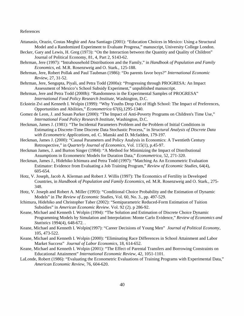
40

References

Attanasio, Orazio, Costas Meghir and Ana Santiago (2001): “Education Choices in Mexico: Using a StructuralModel and a Randomized Experiment to Evaluate Progresa,” manuscript, University College London.

Becker, Gary and Lewis, H. Greg (1973): “On the Interaction between the Quantity and Quality of Children”Journal of Political Economy, 81, 4, Part 2, S143-62.

Behrman, Jere (1997): “Intrahousehold Distributioon and the Family,” in Handbook of Population and FamilyEconomics, ed. M.R. Rosenzweig and O. Stark., 125-188.

Behrman, Jere, Robert Pollak and Paul Taubman (1986): “Do parents favor boys?” International EconomicReview, 27, 31-52.

Behrman, Jere, Sengupta, Piyali, and Petra Todd (2000a): “Progressing through PROGRESA: An ImpactAssessment of Mexico’s School Subsidy Experiment,” unpublished manuscript.

Behrman, Jere and Petra Todd (2000b): “Randomness in the Experimental Samples of PROGRESA” International Food Policy Research Institute, Washington, D.C.

Eckstein Zvi and Kenneth I. Wolpin (1999): “Why Youths Drop Out of High School: The Impact of Preferences,Opportunities and Abilities,” Econometrica 67(6),1295-1340.

Gomez de Leon, J. and Susan Parker (2000): “The Impact of Anti-Poverty Programs on Children's Time Use,” International Food Policy Research Institute, Washington, D.C.

Heckman, James J. (1981): “The Incidental Parameters Problem and the Problem of Initial Conditions inEstimating a Discrete-Time Discrete Data Stochastic Process,” in Structural Analysis of Discrete Datawith Econometric Applications, ed. C. Manski and D. Mcfadden, 179-197.

Heckman, James J. (2000): “Causal Parameters and Policy Analysis in Economics: A Twentieth CenturyRetrospective,” in Quarterly Journal of Economics, Vol. 115(1), p.45-97.

Heckman James, J. and Burton Singer (1984): “A Method for Minimizing the Impact of DistributionalAssumptions in Econometric Models for Duration Data,” Econometrica, 52, 271-320.

Heckman, James J., Hidehiko Ichimura and Petra Todd (1997): “Matching As An Econometric EvaluationEstimator: Evidence from Evaluating a Job Training Program,” Review of Economic Studies, 64(4),605-654.

Hotz, V. Joseph, Jacob A. Klerman and Robert J. Willis (1997): The Economics of Fertility in DevelopedCountries, in Handbook of Population and Family Economics, ed. M.R. Rosenzweig and O. Stark., 275-348.

Hotz, V. Joseph and Robert A. Miller (1993): “Conditional Choice Probability and the Estimation of DynamicModels” in The Review of Economic Studies, Vol. 60, No. 3., pp. 497-529.

Ichimura, Hidehiko and Christopher Taber (2002): “Semiparametric Reduced-Form Estimation of TuitionSubsidies” in American Economic Review. Vol. 92 (2). p 286-92.

Keane, Michael and Kenneth I. Wolpin (1994): “The Solution and Estimation of Discrete Choice DynamicProgramming Models by Simulation and Interpolation: Monte Carlo Evidence,” Review of Economics andStatistics 1994(4), 648-672. .

Keane, Michael and Kenneth I. Wolpin(1997): “Career Decisions of Young Men” Journal of Political Economy,105, 473-522.

Keane, Michael and Kenneth I. Wolpin (2000): “Eliminating Race Differences in School Attainment and LaborMarket Success” Journal of Labor Economics, 18, 614-652.

Keane, Michael and Kenneth I. Wolpin (2001): “The Effect of Parental Transfers and Borrowing Constraints onEducational Attainment” International Economic Review, 42, 1051-1101.

LaLonde, Robert (1986): “Evaluating the Econometric Evaluations of Training Programs with Experimental Data,”American Economic Review, 76, 604-620.

41

Lise, Jeremy, Seitz, Shannon, and Jeffrey Smith (2003): “Equilibrium Policy Experiments and the Evaluation ofSocial Programs,” working paper.

Lumsdaine, Robin L., James H. Stock and David A.Wise (1992): “Pension Plan Provisions and Retirement: Menand Women, Medicare, and Models,” in D. A. Wise (ed.) Studies in the Economics of Aging, Chicago:University of Chicago Press.

Marschak, Jacob (1953): “Economic Measurements for Policy and Prediction,” in William Hood and TjallingKoopmans, eds., Studies in Econometric Method (New York: John Wiley, 1953), pp. 1-26.

McFadden, Daniel (1989): “A Method of Simulated Moments for Estimation of Discrete Response Models withoutNumerical Integration” Econometrica, 57, 5, 995-1026.

Rosenzweig, Mark R. and Kenneth I. Wolpin (1980): “Testing the Quantity-Quality Fertility Model: The Use ofTwins as a Natural Experiment,” Econometrica, 48, 227-40.

Schultz, T. Paul (2000a): “Progresa's Impact on School Enrollments from 1997/98 to 1998/99,” International FoodPolicy Research Institute, Washington, D.C.

Schultz, T. Paul (2000b): “Progresa's Impact on School on School Attendance Rates in the Sampled Population,”International Food Policy Research Institute, Washington, D.C.

Schultz, T. Paul (2000c): “School Subsidies for the Poor: Evaluation a Mexican Strategy for Reducing Poverty,”unpublished manuscript, Yale University.

Skoufias, Emmanuel and Susan Parker (2000): “The Impact of PROGRESA on Work, Liesure and TimeAllocation,” International Food Policy Research Institute, Washington, D.C.

Steinbrickner, Todd E.(2001): “Compensation Policies and Teacher Decisions” International Economic Review,42(3), 751-780.

Willis, Robert J (1973): “A New Approach to the Economic Theory of Fertility Behavior” in Journal of PoliticalEconomy, 81, S12-S64.

Wolpin, Kenneth I. (1999): ‘Commentary on “Analysis of Choice Expectations in Incomplete Scenarios”’ ByCharles F. Manski, Journal of Risk and Uncertainty.

Wolpin, Kenneth I. (1996): “Public Policy Uses of Dynamic Programming Models” American Economic Review,Papers and Proceedings, 86(2), 427-432.

Wolpin, Kenneth I. (1984): “An Estimable Stochastic Model of Fertility and Child Mortality” in The Journal ofPolitical Economy, Vol. 92, No. 5., pp. 852-874.

42

Table 1Monthly transfers for school attendance

under the PROGRESA programSchool Level Grade Monthly Payment in Pesos

Females MalesPrimary 3 70 70

4 80 805 105 1056 135 135

Secondary 1 210 2002 235 2103 255 225

Source: Schultz (1999a, Table 1). Corresponds to first term of the 1998-99 schoolyear.

Table 2Means and standard deviations of selected variables

MeanStandardDeviation

Wife’s age in 1997 30.5 8.1Husband’s age in 1997 34.4 9.5Wife’s age at marriage 18.1 3.4Number of children ever born (1997 ) 3.01 1.92Number of children ever born (1998) 3.06 1.84Number of children ever born to women age 35-49 (1997)

4.05 2.14

Highest grade completed of children age 7-11 2.39 1.41Highest grade completed of children aged 12-15 5.79 1.76

Highest grade completed of children age 16 or older All Boys Girls

6.606.646.56

2.812.822.81

Percentage with secondary school in Village 26.7Distance to secondary school if not in Village (km) 2.82 1.60Distance to city (km) 136 74Parent’s income (pesos) 11,841 12,551Percentage of children aged 12-15 who worked for pay

8.4 -

Market income of working children age:

12 5605 331013 6707 267114 8037 741515 9073 9549

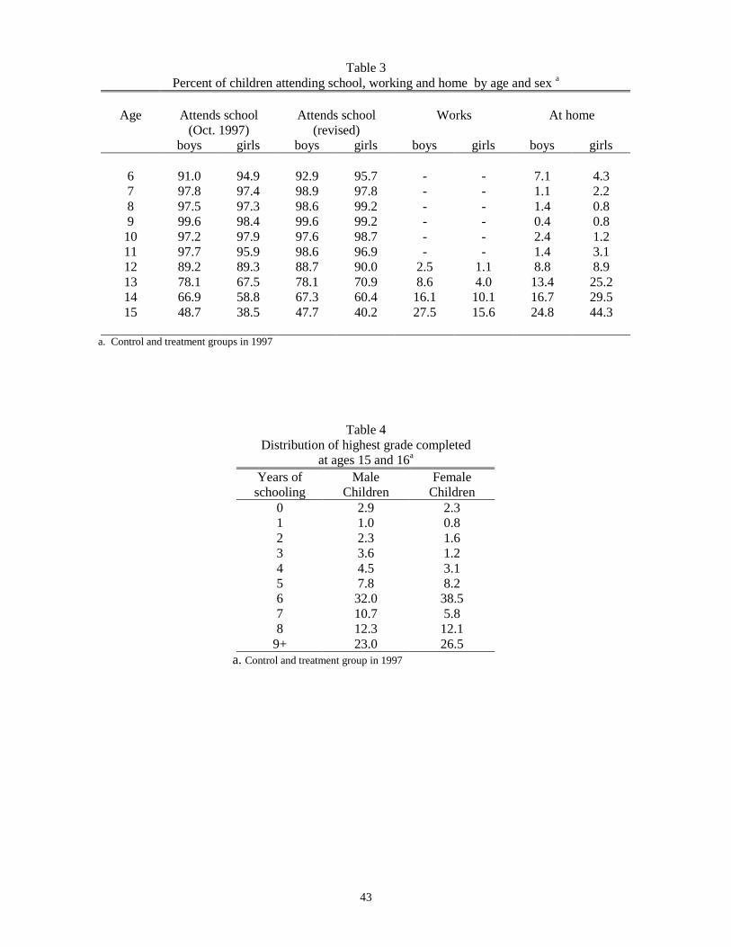
43

Table 3Percent of children attending school, working and home by age and sex a

Age Attends school(Oct. 1997)

Attends school(revised)

Works At home

boys girls boys girls boys girls boys girls

6 91.0 94.9 92.9 95.7 - - 7.1 4.37 97.8 97.4 98.9 97.8 - - 1.1 2.28 97.5 97.3 98.6 99.2 - - 1.4 0.89 99.6 98.4 99.6 99.2 - - 0.4 0.810 97.2 97.9 97.6 98.7 - - 2.4 1.211 97.7 95.9 98.6 96.9 - - 1.4 3.112 89.2 89.3 88.7 90.0 2.5 1.1 8.8 8.913 78.1 67.5 78.1 70.9 8.6 4.0 13.4 25.214 66.9 58.8 67.3 60.4 16.1 10.1 16.7 29.515 48.7 38.5 47.7 40.2 27.5 15.6 24.8 44.3

a. Control and treatment groups in 1997

Table 4Distribution of highest grade completed

at ages 15 and 16a

Years ofschooling

MaleChildren

FemaleChildren

0 2.9 2.31 1.0 0.82 2.3 1.63 3.6 1.24 4.5 3.15 7.8 8.26 32.0 38.57 10.7 5.88 12.3 12.1

9+ 23.0 26.5a. Control and treatment group in 1997

44

Table 5Distribution of the durations from marriage

to first, second and third birtha

Duration frommarriage(years)

To FirstBirth

ToSecondBirth

To ThirdBirth

1 52.4 - -2 18.5 10.6 -3 9.7 24.5 1.74 4.6 18.6 8.95 3.4 11.9 16.06 2.5 8.3 15.47 1.5 6.4 12.48 1.4 4.2 10.19 1.3 3.3 8.010 1.1 2.2 6.611 0.8 1.8 4.5

12+ 2.7 8.2 16.5a. Control and treatment groups in 1997

Table 6One period transition rates by sex: age(a) 13 to 15

BoysHome (a) Work (a) School (a)

Home (a-1) 44.4 40.7 14.8Work (a-1) 25.0 62.5 12.5School (a-1) 8.3 5.5 86.2

GirlsHome (a) Work (a) School (a)

Home (a-1) 92.5 7.5 0.0Work (a-1) 40.0 20.0 20.0School (a-1) 21.5 1.5 76.9

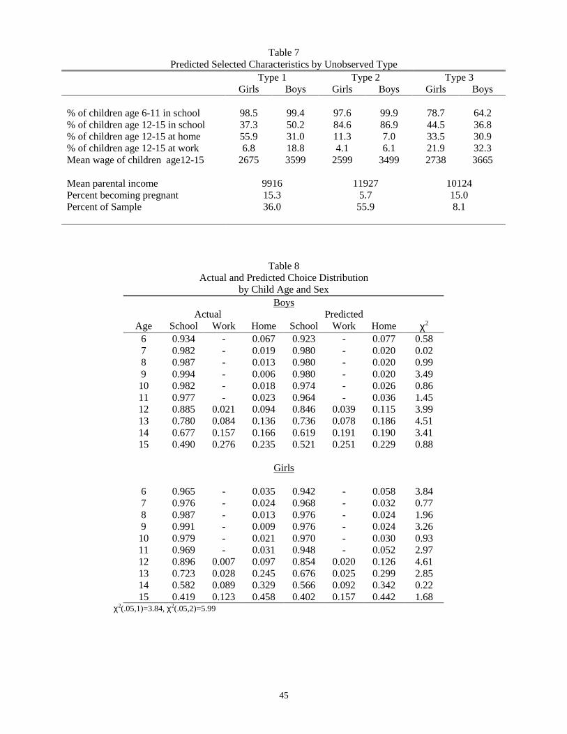
45

Table 7Predicted Selected Characteristics by Unobserved Type

Type 1 Type 2 Type 3Girls Boys Girls Boys Girls Boys

% of children age 6-11 in school 98.5 99.4 97.6 99.9 78.7 64.2% of children age 12-15 in school 37.3 50.2 84.6 86.9 44.5 36.8% of children age 12-15 at home 55.9 31.0 11.3 7.0 33.5 30.9% of children age 12-15 at work 6.8 18.8 4.1 6.1 21.9 32.3Mean wage of children age12-15 2675 3599 2599 3499 2738 3665

Mean parental income 9916 11927 10124Percent becoming pregnant 15.3 5.7 15.0Percent of Sample 36.0 55.9 8.1

Table 8Actual and Predicted Choice Distribution

by Child Age and SexBoys

Actual PredictedAge School Work Home School Work Home χ2

6 0.934 - 0.067 0.923 - 0.077 0.587 0.982 - 0.019 0.980 - 0.020 0.028 0.987 - 0.013 0.980 - 0.020 0.999 0.994 - 0.006 0.980 - 0.020 3.4910 0.982 - 0.018 0.974 - 0.026 0.8611 0.977 - 0.023 0.964 - 0.036 1.4512 0.885 0.021 0.094 0.846 0.039 0.115 3.9913 0.780 0.084 0.136 0.736 0.078 0.186 4.5114 0.677 0.157 0.166 0.619 0.191 0.190 3.4115 0.490 0.276 0.235 0.521 0.251 0.229 0.88

Girls

6 0.965 - 0.035 0.942 - 0.058 3.847 0.976 - 0.024 0.968 - 0.032 0.778 0.987 - 0.013 0.976 - 0.024 1.969 0.991 - 0.009 0.976 - 0.024 3.2610 0.979 - 0.021 0.970 - 0.030 0.9311 0.969 - 0.031 0.948 - 0.052 2.9712 0.896 0.007 0.097 0.854 0.020 0.126 4.6113 0.723 0.028 0.245 0.676 0.025 0.299 2.8514 0.582 0.089 0.329 0.566 0.092 0.342 0.2215 0.419 0.123 0.458 0.402 0.157 0.442 1.68

χ2(.05,1)=3.84, χ2(.05,2)=5.99

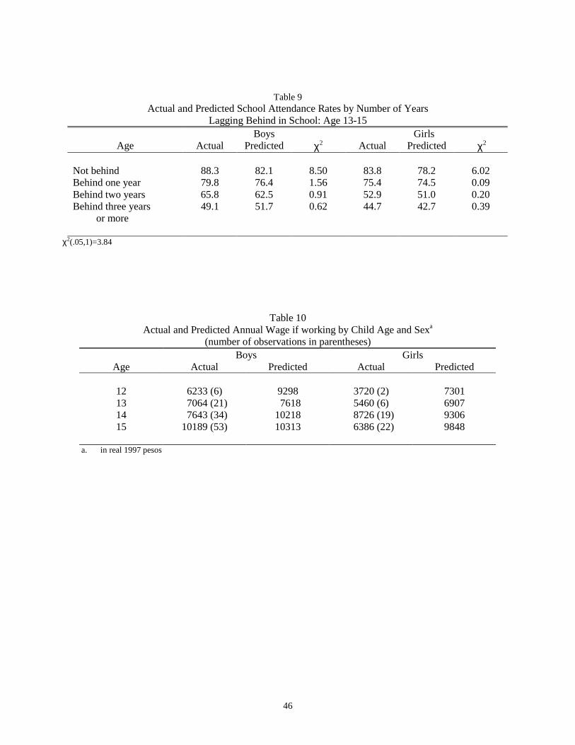
46

Table 9Actual and Predicted School Attendance Rates by Number of Years

Lagging Behind in School: Age 13-15Boys Girls

Age Actual Predicted χ2 Actual Predicted χ2

Not behind 88.3 82.1 8.50 83.8 78.2 6.02Behind one year 79.8 76.4 1.56 75.4 74.5 0.09Behind two years 65.8 62.5 0.91 52.9 51.0 0.20Behind three years or more

49.1 51.7 0.62 44.7 42.7 0.39

χ2(.05,1)=3.84

Table 10Actual and Predicted Annual Wage if working by Child Age and Sexa

(number of observations in parentheses)Boys Girls

Age Actual Predicted Actual Predicted

12 6233 (6) 9298 3720 (2) 730113 7064 (21) 7618 5460 (6) 690714 7643 (34) 10218 8726 (19) 930615 10189 (53) 10313 6386 (22) 9848

a. in real 1997 pesos

47

Table 11Actual and Predicted School Attendance Rates by Child

Age, Sex and School Attainment: Control and Treatment Groups by Yeara

Girls BoysControl Group Treatment Group Control Group Treatment Group

1997 1998 1997 1998 1997 1998 1997 1998Age 6-11 Actual 96.9 96.5 97.6 98.5b 96.6 96.7 97.6 98.7b

Predicted 96.1 96.2 96.4 97.1 96.4 96.4 96.3 97.1 No. obs. 449 431 632 600 471 460 671 678

Age 12-15 Actual 65.3 66.5 62.9 74.4b,c,d 68.8 72.5 69.5 76.3c

Predicted 61.6 61.8 61.8 74.9 68.8 68.8 68.0 77.1 No. obs. 190 176 205 223 189 182 279 262

Age 12-15, Behind in School Actual 58.3 58.7 56.9 71.4b,c,d 64.0 67.4 64.2 71.6c

Predicted 54.2 55.5 55.6 72.3 63.9 65.3 62.7 72.9 No. obs. 127 121 144 161 139 135 204 190

Age 13-15, HGC≥6Behind in School Actual 40.9 44.4 30.3 51.5c,d 59.0 57.1 52.6 58.3 Predicted 40.2 45.3 37.3 58.7 55.0 53.0 51.7 66.7 No. obs. 66 72 66 66 61 56 95 96

a. based on 200 simulation draws per familyb. cross-section treatment effect (T98-C98) p-value ≤ .10c. longitudinal treatment effect (T98-T97) p-value ≤ .10d. difference-in-difference treatment effect ((T98-T97) – (C98-C97)) p-value ≤ .10

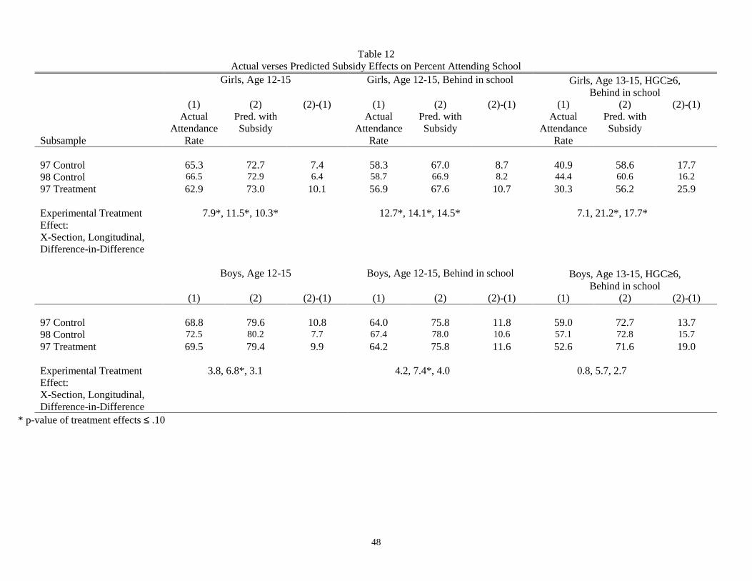
48

Table 12Actual verses Predicted Subsidy Effects on Percent Attending School

Girls, Age 12-15 Girls, Age 12-15, Behind in school Girls, Age 13-15, HGC≥6,Behind in school

Subsample

(1)Actual

AttendanceRate

(2)Pred. withSubsidy

(2)-(1) (1)Actual

AttendanceRate

(2)Pred. withSubsidy

(2)-(1) (1)Actual

AttendanceRate

(2)Pred. withSubsidy

(2)-(1)

97 Control 65.3 72.7 7.4 58.3 67.0 8.7 40.9 58.6 17.798 Control 66.5 72.9 6.4 58.7 66.9 8.2 44.4 60.6 16.297 Treatment 62.9 73.0 10.1 56.9 67.6 10.7 30.3 56.2 25.9

Experimental TreatmentEffect:X-Section, Longitudinal,Difference-in-Difference

7.9*, 11.5*, 10.3* 12.7*, 14.1*, 14.5* 7.1, 21.2*, 17.7*

Boys, Age 12-15 Boys, Age 12-15, Behind in school Boys, Age 13-15, HGC≥6,Behind in school

(1) (2) (2)-(1) (1) (2) (2)-(1) (1) (2) (2)-(1)

97 Control 68.8 79.6 10.8 64.0 75.8 11.8 59.0 72.7 13.798 Control 72.5 80.2 7.7 67.4 78.0 10.6 57.1 72.8 15.797 Treatment 69.5 79.4 9.9 64.2 75.8 11.6 52.6 71.6 19.0

Experimental TreatmentEffect:X-Section, Longitudinal,Difference-in-Difference

3.8, 6.8*, 3.1 4.2, 7.4*, 4.0 0.8, 5.7, 2.7

* p-value of treatment effects ≤ .10

49

Table 13Actual and Predicted Choice Distribution by Child

Age, Sex and School Attainment: Post-Subsidy Treatment

Girls Boys

In School Home Work In School Home WorkActa Predb Act. Pred. Act. Pred. Act. Pred. Act. Pred. Act. Pred.

Age 12-15c,d

All 74.4 74.9 21.2 22.3 4.1 2.8 76.3 77.1 14.9 15.0 8.8 7.9 Not Behind 82.3 82.1 14.5 14.8 3.2 3.1 88.9 88.2 9.7 9.7 1.4 2.1 Behind 71.9 72.3 23.7 25.0 4.4 2.7 71.6 72.9 16.8 16.9 11.6 10.2 Not Behind and 52.3 58.7 41.5 37.7 6.2 3.6 58.3 66.7 25.0 20.9 16.7 12.4 HGC ≥ 6a. Based on observations in which neither the school nor work choice is missing.b. Based in all observations including those missing school or work.c. Numbers of observations for each of the four rows are 222, 62, 160 and 65 for girls, and 262, 72, 190 and 96 for boys.d. Based on 200 simulation draws per family.

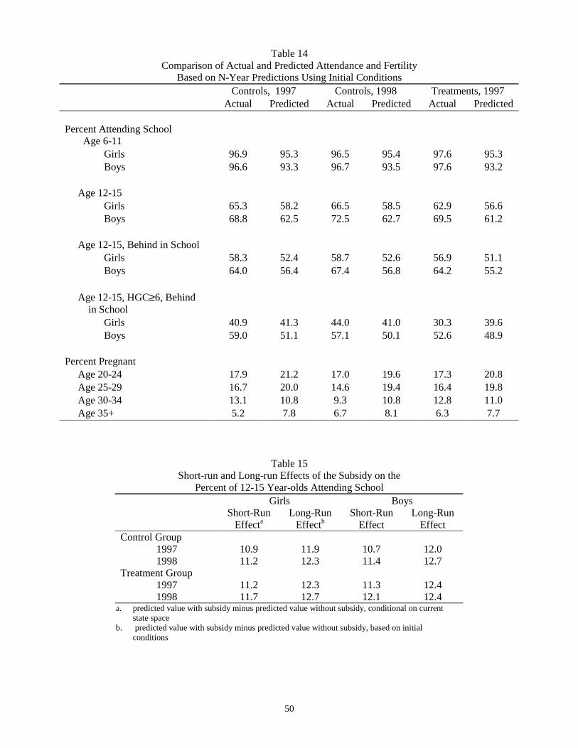
50

Table 14Comparison of Actual and Predicted Attendance and Fertility

Based on N-Year Predictions Using Initial ConditionsControls, 1997 Controls, 1998 Treatments, 1997

Actual Predicted Actual Predicted Actual Predicted

Percent Attending School Age 6-11 Girls 96.9 95.3 96.5 95.4 97.6 95.3 Boys 96.6 93.3 96.7 93.5 97.6 93.2

Age 12-15 Girls 65.3 58.2 66.5 58.5 62.9 56.6 Boys 68.8 62.5 72.5 62.7 69.5 61.2

Age 12-15, Behind in School Girls 58.3 52.4 58.7 52.6 56.9 51.1 Boys 64.0 56.4 67.4 56.8 64.2 55.2

Age 12-15, HGC≥6, Behind in School Girls 40.9 41.3 44.0 41.0 30.3 39.6 Boys 59.0 51.1 57.1 50.1 52.6 48.9

Percent Pregnant Age 20-24 17.9 21.2 17.0 19.6 17.3 20.8 Age 25-29 16.7 20.0 14.6 19.4 16.4 19.8 Age 30-34 13.1 10.8 9.3 10.8 12.8 11.0 Age 35+ 5.2 7.8 6.7 8.1 6.3 7.7

Table 15Short-run and Long-run Effects of the Subsidy on the

Percent of 12-15 Year-olds Attending SchoolGirls Boys

Short-Run Long-Run Short-Run Long-RunEffecta Effectb Effect Effect

Control Group1997 10.9 11.9 10.7 12.01998 11.2 12.3 11.4 12.7

Treatment Group1997 11.2 12.3 11.3 12.41998 11.7 12.7 12.1 12.4

a. predicted value with subsidy minus predicted value without subsidy, conditional on currentstate space

b. predicted value with subsidy minus predicted value without subsidy, based on initialconditions

51

Table 16Predicted Effect of the Subsidy on Completed Schooling of Children by Age 16:

All Children Ever Borna

Girls BoysNo Subsidy Subsidy No Subsidy Subsidy

Mean Schooling 6.29 6.83 6.42 6.96

Percent Completing 75.8 82.2 78.8 83.3 Grade Six or More

Percent Completing 19.8 25.8 22.8 28.1 Grade Nine or More

a. completed schooling at grade 10

Table 17Predicted Effect of Subsidy on Completed Fertility:

All Children Ever BornWithoutsubsidy

Withsubsidy

Mean Number of Children Ever Born 4.24 4.28

Percent of Families with Zero Children 0.05 0.04 One Child 1.16 1.13 Two Children 9.23 8.74 Three Children 22.97 22.48 Four Children 24.43 24.60 Five Children 21.54 21.46 Six Children 14.78 15.30 Seven Children 5.05 5.36

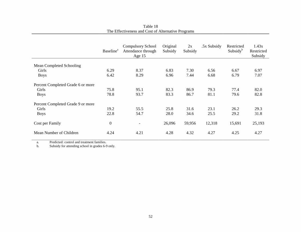
52

Table 18The Effectiveness and Cost of Alternative Programs

BaselineaCompulsory SchoolAttendance through

Age 15

OriginalSubsidy

2xSubsidy

.5x Subsidy RestrictedSubsidyb

1.43xRestrictedSubsidy

Mean Completed Schooling Girls 6.29 8.37 6.83 7.30 6.56 6.67 6.97 Boys 6.42 8.29 6.96 7.44 6.68 6.79 7.07

Percent Completed Grade 6 or more Girls 75.8 95.1 82.3 86.9 79.3 77.4 82.0 Boys 78.8 93.7 83.3 86.7 81.1 79.6 82.8

Percent Completed Grade 9 or more Girls 19.2 55.5 25.8 31.6 23.1 26.2 29.3 Boys 22.8 54.7 28.0 34.6 25.5 29.2 31.8

Cost per Family 0 - 26,096 59,956 12,318 15,691 25,193

Mean Number of Children 4.24 4.21 4.28 4.32 4.27 4.25 4.27

a. Predicted: control and treatment families.b. Subsidy for attending school in grades 6-9 only.

53

Table 18 continuedThe Effectiveness and Cost of Alternative Programs

Bonus forCompleting 9th

Gradec

Junior SecondarySchool in Each

Village

UnconditionalIncome Transfer5,000 Pesos /Yr

No Child Laborthrough Age 15

Original Subsidyand 25%

Wage Increase

Mean Completed Schooling Girls 6.50 6.39 6.41 6.30 6.75 Boys 6.58 6.55 6.53 6.52 6.79

Percent Completed Grade 6 or more Girls 74.9 76.0 77.6 76.1 81.5 Boys 76.9 79.0 80.0 79.9 81.8

Percent Completed Grade 9 or more Girls 28.8 21.2 20.8 19.7 25.3 Boys 32.7 24.1 23.6 23.5 26.5

Cost per Family 36,996 - 237,000 - 25,262

Mean Number Children 4.20 4.25 4.23 4.25 4.29

c. The bonus is set at 30,000 pesos for girls and boys.

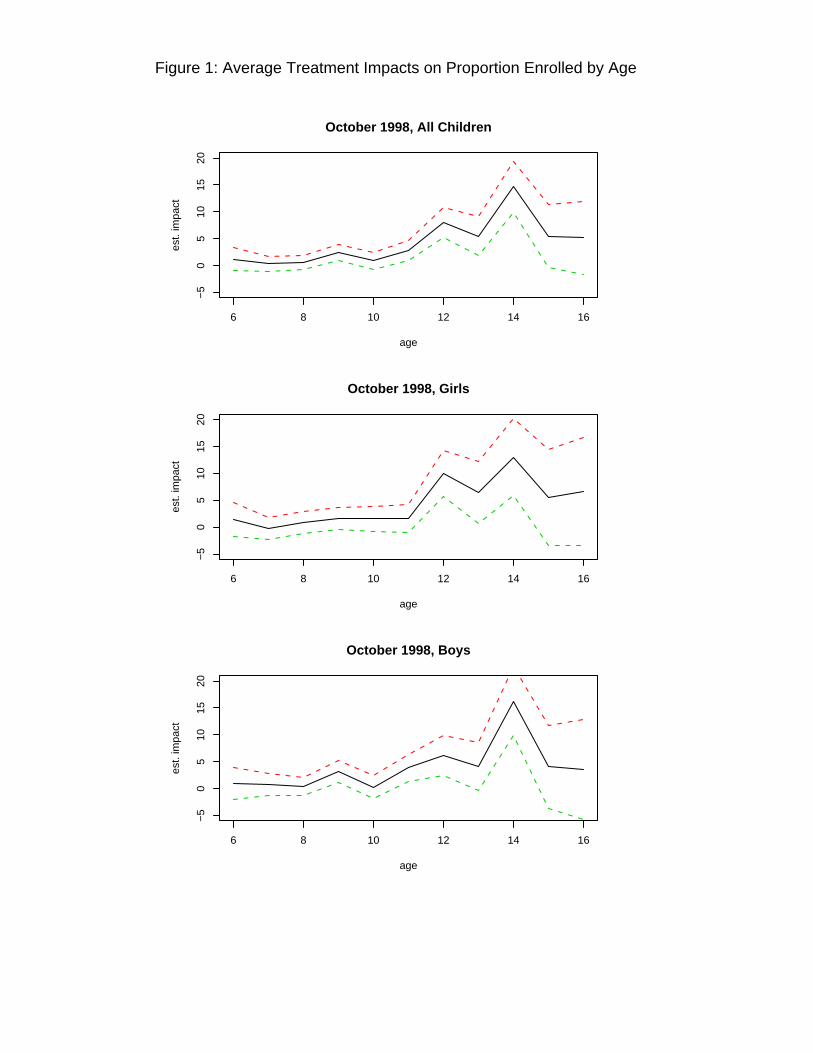
6 8 10 12 14 16

−5

05

1015

20

age

est.

impa

ct

October 1998, All Children

6 8 10 12 14 16

−5

05

1015

20

age

est.

impa

ct

October 1998, Girls

6 8 10 12 14 16

−5

05

1015

20

age

est.

impa

ct

October 1998, Boys

Figure 1: Average Treatment Impacts on Proportion Enrolled by Age

(A.1)

ut 100

C(t)00[1exp(01N(t1)02S(t)03 (15

j12l(t, tj)n(tj)]

(3

j11, jI(typej)N(t) (

3

j12, jI(typej)N(t)2

(3

j13, jI(typej) S(t)

(3

j14, jI(typej)N(t) S(t)5(

3

j1n(tj)6(

3

j1n(tj)2

(3

j17, jI(typej)(

nI(S(t,-n)6)

(3

j18, jI(typej)(

nI(S(t,-n)9)9I(p(tm)1)10I( (

24

t20p(t)1)11I( (

29

t25p(t)1)

12I( (34

t30p(t)1)13I( (

39

t35p(t)1)14I( (

43

t40p(t)1)15I(p(t1)1)I(p(t)1)

16 (15

k12I(Sb(t,-n)6,sb(t,-n)1) t-nk))17 (

15

k12I(Sg(t,-n)6,sg(t,-n)1) t-nk)

19, j (3

j1I(typej) (

15

k12I(S(t,-n)(t-n6)1,s(t,-n)1) t-nk))

20 (15

k12I(S(t,-n)(t-n6)2,s(t,-n)1) t-nk))

21 (15

k12I(S(t,-n)(t-n6)3,s(t,-n)1) t-nk))

22 (15

k12I(Sb(t,-n)(t-n6)0,sb(t,-n)1) t-nk))

A.1

Appendix A

Utility function:

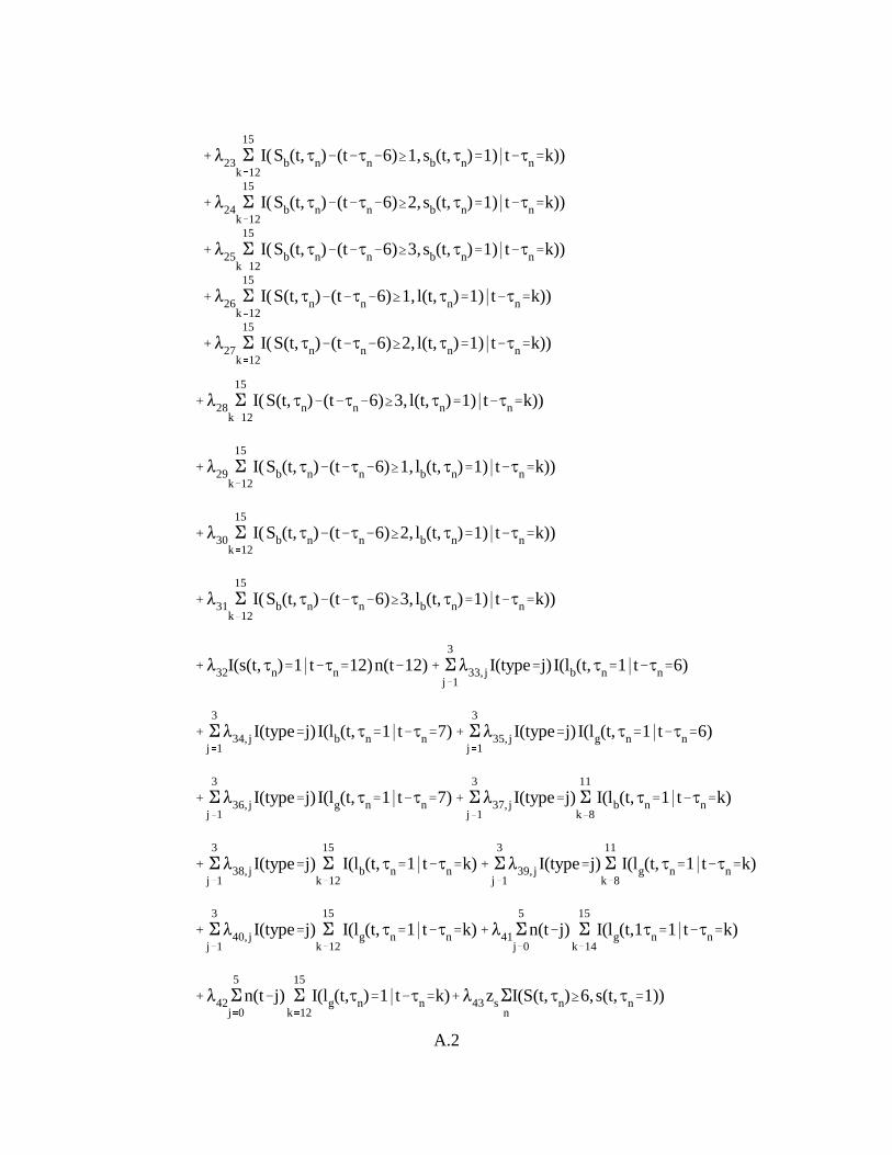
23 (15

k12I(Sb(t,-n)(t-n6)1,sb(t,-n)1) t-nk))

24 (15

k12I(Sb(t,-n)(t-n6)2,sb(t,-n)1) t-nk))

25 (15

k12I(Sb(t,-n)(t-n6)3,sb(t,-n)1) t-nk))

26 (15

k12I(S(t,-n)(t-n6)1, l(t,-n)1) t-nk))

27 (15

k12I(S(t,-n)(t-n6)2, l(t,-n)1) t-nk))

28 (15

k12I(S(t,-n)(t-n6)3, l(t,-n)1) t-nk))

29 (15

k12I(Sb(t,-n)(t-n6)1, lb(t,-n)1) t-nk))

30 (15

k12I(Sb(t,-n)(t-n6)2, lb(t,-n)1) t-nk))

31 (15

k12I(Sb(t,-n)(t-n6)3, lb(t,-n)1) t-nk))

32I(s(t,-n)1 t-n12)n(t12) (3

j133, jI(typej) I(l b(t,-n1 t-n6)

(3

j134, jI(typej) I(l b(t,-n1 t-n7) (

3

j135, jI(typej) I(l g(t,-n1 t-n6)

(3

j136, jI(typej) I(l g(t,-n1 t-n7) (

3

j137, jI(typej) (

11

k8I(l b(t,-n1 t-nk)

(3

j138, jI(typej) (

15

k12I(l b(t,-n1 t-nk) (

3

j139, jI(typej) (

11

k8I(l g(t,-n1 t-nk)

(3

j140, jI(typej) (

15

k12I(l g(t,-n1 t-nk)41(

5

j0n(tj) (

15

k14I(l g(t,1-n1 t-nk)

42(5

j0n(tj) (

15

k12I(l g(t,-n)1 t-nk)43zs(

nI(S(t,-n)6,s(t,-n1))

A.2

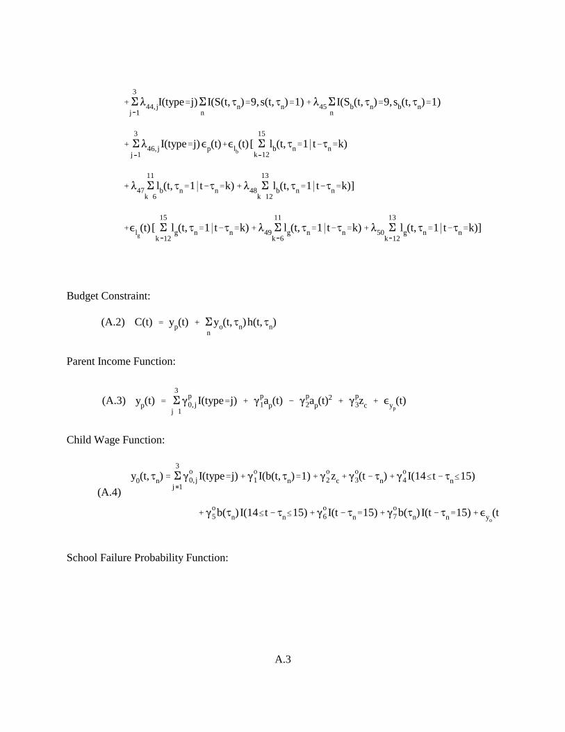
(3

j144, jI(typej)(

nI(S(t,-n)9,s(t,-n)1)45(

nI(Sb(t,-n)9,sb(t,-n)1)

(3

j146, jI(typej) p(t)lb

(t) [ (15

k12lb(t,-n1 t-nk)

47(11

k6lb(t,-n1 t-nk)48 (

13

k12lb(t,-n1 t-nk)]

lg(t) [ (

15

k12lg(t,-n1 t-nk)49(

11

k6lg(t,-n1 t-nk)50 (

13

k12lg(t,-n1 t-nk)]

(A.2) C(t) yp(t) (n

yo(t,-n)h(t,-n)

(A.3) yp(t) (3

j1

p0, j I(typej)

p1ap(t)

p2ap(t)

2

p3zc yp

(t)

(A.4)

y0(t,-n) (3

j1

o0, j I(typej)o

1I(b(t,-n)1)o2zc

o3(t-n)

o4I(14t-n15)

o5b(-n) I(14t-n15)o

6I(t-n15)o7b(-n) I(t-n15)yo

(t)

A.3

Budget Constraint:

Parent Income Function:

Child Wage Function:

School Failure Probability Function:

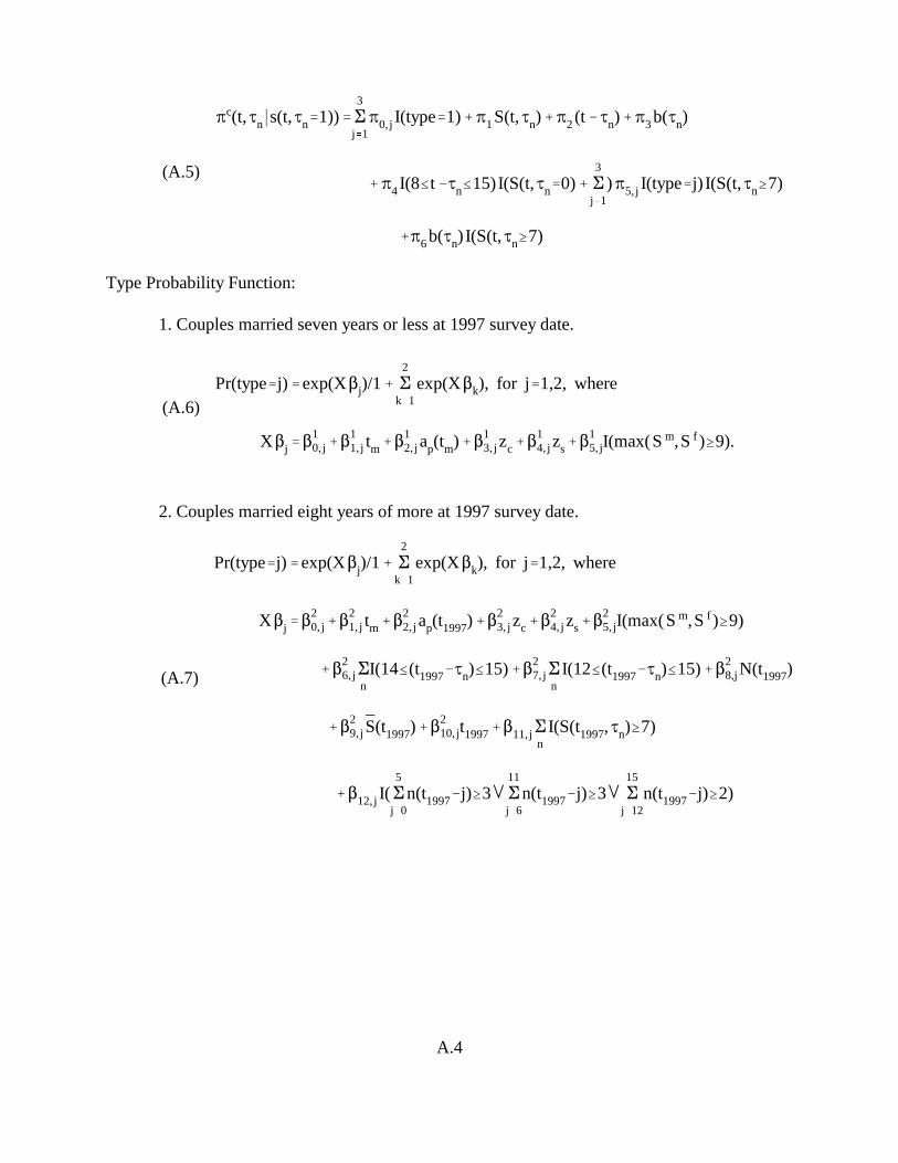
(A.5)

%c(t,-n s(t,-n1))(3

j1%0, j I(type1)%1S(t,-n)%2(t-n)%3b(-n)

%4I(8t-n15)I(S(t,-n0) (3

j1)%5, j I(typej) I(S(t,-n7)

%6b(-n) I(S(t,-n7)

(A.6)Pr(typej)exp(Xj)/1 (

2

k1exp(Xk), for j1,2, where

Xj10, j

11, j tm

12, jap(tm)1

3, jzc14, jzs

15, jI(max(Sm,Sf )9).

(A.7)

Pr(typej)exp(Xj)/1 (2

k1exp(Xk), for j1,2, where

Xj20, j

21, j tm

22, jap(t1997)

23, jzc

24, jzs

25, jI(max(Sm,Sf )9)

26, j(

nI(14(t1997-n)15)2

7, j(n

I(12(t1997-n)15)28,jN(t1997)

29, j S(t1997)

210, jt199711, j(

nI(S(t1997,-n)7)

12, jI((5

j0n(t1997j)3 (

11

j6n(t1997j)3 (

15

j12n(t1997j)2)

A.4

Type Probability Function:

1. Couples married seven years or less at 1997 survey date.

2. Couples married eight years of more at 1997 survey date.

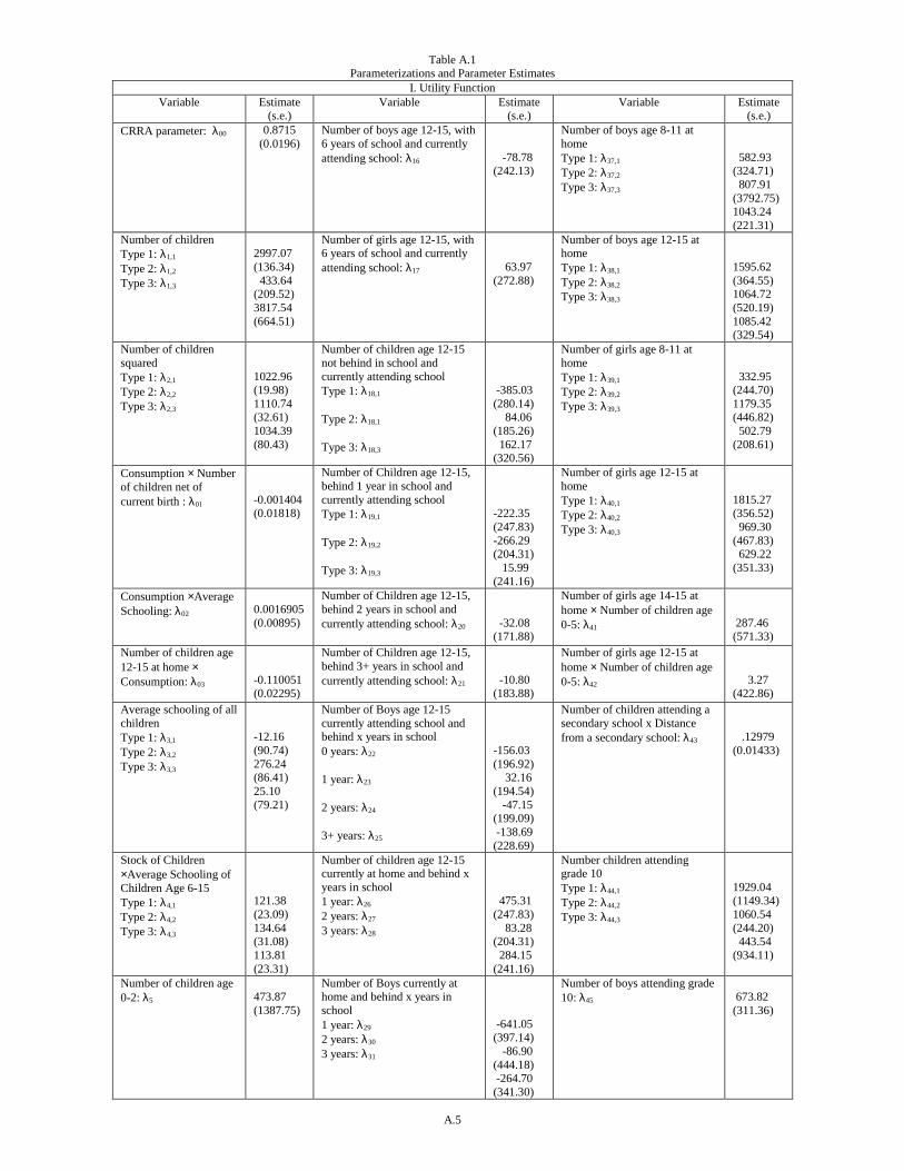
Table A.1Parameterizations and Parameter Estimates

I. Utility FunctionVariable Estimate

(s.e.)Variable Estimate

(s.e.)Variable Estimate

(s.e.)CRRA parameter: λ00 0.8715

(0.0196)Number of boys age 12-15, with6 years of school and currentlyattending school: λ16 -78.78

(242.13)

Number of boys age 8-11 athomeType 1: λ37,1

Type 2: λ37,2

Type 3: λ37,3

582.93(324.71) 807.91(3792.75)1043.24(221.31)

Number of childrenType 1: λ1,1

Type 2: λ1,2

Type 3: λ1,3

2997.07(136.34) 433.64(209.52)3817.54(664.51)

Number of girls age 12-15, with6 years of school and currentlyattending school: λ17 63.97

(272.88)

Number of boys age 12-15 athomeType 1: λ38,1

Type 2: λ38,2

Type 3: λ38,3

1595.62(364.55)1064.72(520.19)1085.42(329.54)

Number of childrensquaredType 1: λ2,1

Type 2: λ2,2

Type 3: λ2,3

1022.96(19.98)1110.74(32.61)1034.39(80.43)

Number of children age 12-15not behind in school andcurrently attending schoolType 1: λ18,1

Type 2: λ18,1

Type 3: λ18,3

-385.03(280.14) 84.06(185.26) 162.17(320.56)

Number of girls age 8-11 athomeType 1: λ39,1

Type 2: λ39,2

Type 3: λ39,3

332.95(244.70)1179.35(446.82) 502.79(208.61)

Consumption × Numberof children net ofcurrent birth : λ01 -0.001404

(0.01818)

Number of Children age 12-15,behind 1 year in school andcurrently attending schoolType 1: λ19,1

Type 2: λ19,2

Type 3: λ19,3

-222.35(247.83)-266.29(204.31) 15.99(241.16)

Number of girls age 12-15 athomeType 1: λ40,1

Type 2: λ40,2

Type 3: λ40,3

1815.27(356.52) 969.30(467.83) 629.22(351.33)

Consumption ×AverageSchooling: λ02 0.0016905

(0.00895)

Number of Children age 12-15,behind 2 years in school andcurrently attending school: λ20 -32.08

(171.88)

Number of girls age 14-15 athome × Number of children age0-5: λ41 287.46

(571.33)Number of children age12-15 at home ×Consumption: λ03 -0.110051

(0.02295)

Number of Children age 12-15,behind 3+ years in school andcurrently attending school: λ21 -10.80

(183.88)

Number of girls age 12-15 athome × Number of children age0-5: λ42 3.27

(422.86)Average schooling of allchildrenType 1: λ3,1

Type 2: λ3,2

Type 3: λ3,3

-12.16(90.74)276.24(86.41)25.10(79.21)

Number of Boys age 12-15currently attending school andbehind x years in school0 years: λ22

1 year: λ23

2 years: λ24

3+ years: λ25

-156.03(196.92) 32.16(194.54) -47.15(199.09) -138.69(228.69)

Number of children attending asecondary school x Distancefrom a secondary school: λ43 .12979

(0.01433)

Stock of Children×Average Schooling ofChildren Age 6-15Type 1: λ4,1

Type 2: λ4,2

Type 3: λ4,3

121.38(23.09)134.64(31.08)113.81(23.31)

Number of children age 12-15currently at home and behind xyears in school1 year: λ26

2 years: λ27

3 years: λ28

475.31(247.83) 83.28(204.31) 284.15(241.16)

Number children attendinggrade 10Type 1: λ44,1

Type 2: λ44,2

Type 3: λ44,3

1929.04(1149.34)1060.54(244.20) 443.54(934.11)

Number of children age0-2: λ5 473.87

(1387.75)

Number of Boys currently athome and behind x years inschool1 year: λ29

2 years: λ30

3 years: λ31

-641.05(397.14) -86.90(444.18) -264.70(341.30)

Number of boys attending grade10: λ45 673.82

(311.36)

A.5

Table A.1, continuedParameterizations and Parameter Estimates

I. Utility Function continued.Variable Estimate

(s.e.)Variable Estimate

(s.e.)Variable Estimate

(s.e.)Number of children age0-2 squared : λ6 -811.75

(544.91)Age 12 and in school: λ32 186.85

(199.21)

Pregnancy shockType 1: λ46,1

Type 2: λ46,2

Type 3: λ46,3

1.00.90674

(0.03192)0.97329

(0.12767)Number of Childrenwith 6 or more years ofschoolingType 1: λ7,1

Type 2: λ7,2

Type 3: λ7,3

184.63(39.38)11.50

(35.49)-54.21(22.98)

Boy age 6 at homeType 1: λ33,1

Type 2: λ33,2

Type 3: λ33,3

1205.91(362.39) 1421.85(1681.07) 1579.79(323.36)

Shock to preferences for boysage 12 –15 at home x number ofboys at home age 6-11: λ47

12-13: λ48

0.31036(228.51)-0.11917(0.1373)

Number of Childrenwith 9 or more years ofschoolingType 1: λ8,1

Type 2: λ8,2

Type 3: λ8,3

1.43(48.65)147.43(41.84)

6.06(42.96)

Boy age 7 at homeType 1: λ34,1

Type 2: λ34,2

Type 3: λ34,3

697.49(2161.71) 644.18(3.34E6) 935.43(234.52)

Shock to preferences for girlsage 12 –15 at home x number ofgirls at home age 6-11: λ49

12-13: λ50

.87932(217.73) -.24124(0.1510)

Pregnancy at:First yr. of marriage: λ9

Age 20-24: λ19

25-29: λ11

30-34: λ12

35-39: λ13

40-43: λ14

31834.43(1312.82) -1126.39(1030.11) -3071.81(2030.60)-24413.72(1355.16)-27203.99(2030.60)-59672.14(7098.44)

Girl age 6 at homeType 1: λ35,1

Type 2: λ35,2

Type 3: λ35,3

582.94(822.72)1676.45(387.47) 885.99(272.70)

Pregnancy× Pregnancyin previous period : λ15 -37001.59

(1442.54)

Girl age 7 at homeType 1: λ36,1

Type 2: λ36,2

Type 3: λ36,3

356.10(462.73)1072.03(1231.52) 680.21(382.96)

(a) the discount rate δ is set equal to 0.95

A.6

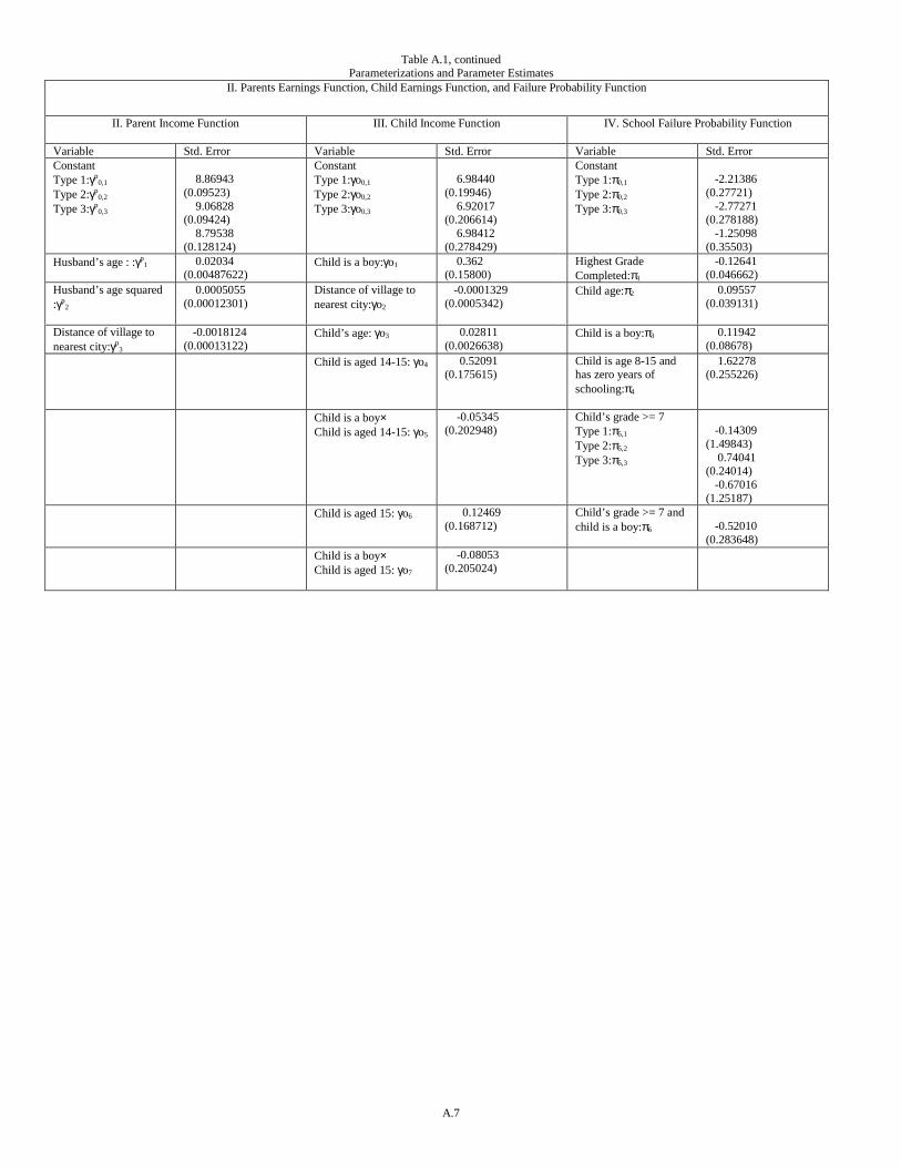
Table A.1, continuedParameterizations and Parameter Estimates

II. Parents Earnings Function, Child Earnings Function, and Failure Probability Function

II. Parent Income Function III. Child Income Function IV. School Failure Probability Function

Variable Std. Error Variable Std. Error Variable Std. ErrorConstantType 1:γp

0,1

Type 2:γp0,2

Type 3:γp0,3

8.86943(0.09523) 9.06828(0.09424) 8.79538(0.128124)

ConstantType 1:γo0,1

Type 2:γo0,2

Type 3:γo0,3

6.98440(0.19946) 6.92017(0.206614) 6.98412(0.278429)

ConstantType 1:π0,1

Type 2:π0,2

Type 3:π0,3

-2.21386(0.27721) -2.77271(0.278188) -1.25098(0.35503)

Husband’s age : :γp1 0.02034

(0.00487622)Child is a boy:γo1 0.362

(0.15800)Highest GradeCompleted:π1

-0.12641(0.046662)

Husband’s age squared:γp

2

0.0005055(0.00012301)

Distance of village tonearest city:γo2

-0.0001329(0.0005342)

Child age:π2 0.09557(0.039131)

Distance of village tonearest city:γp

3

-0.0018124(0.00013122)

Child’s age: γo3 0.02811(0.0026638)

Child is a boy:π3 0.11942(0.08678)

Child is aged 14-15: γo4 0.52091(0.175615)

Child is age 8-15 andhas zero years ofschooling:π4

1.62278(0.255226)

Child is a boy×Child is aged 14-15: γo5

-0.05345(0.202948)

Child’s grade >= 7Type 1:π5,1

Type 2:π5,2

Type 3:π5,3

-0.14309(1.49843) 0.74041(0.24014) -0.67016(1.25187)

Child is aged 15: γo6 0.12469(0.168712)

Child’s grade >= 7 andchild is a boy:π6 -0.52010

(0.283648)Child is a boy×Child is aged 15: γo7

-0.08053(0.205024)

A.7

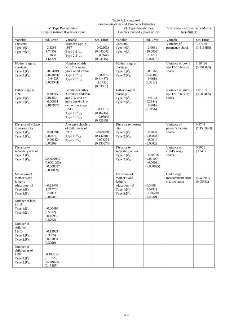
Table A.1, continuedParameterizations and Parameter Estimates

V. Type Probabilities:Couples married 8 years or more

VI. Type Probabilities:Couples married 7 years or less

VII. Variance-Covariance Matrixf(ε)=N(0,Ω)

Variable Std. Error Variable Std. Error Variable Std. Error Variable Std. ErrorConstantType 1:β2

0,1

Type 2:β20,2

2.5289(1.7435) 1.7650(1.6122)

Mother’s age in1997Type 1:β2

10,1

Type 2:β210,2

-0.029033(0.04564) 0.009445(0.04145)

ConstantType 1:β1

0,1

Type 2:β10,2

2.0681(10.0052) 1.1235(9.07815)

Variance ofpregnancy shock

3.274E9(1.5114E8)

Mother’s age atmarriageType 1:β2

1,1

Type 2:β21,2

-0.04049(0.072084) 0.04235(0.059344)

Number of kidswith 7 or moreyears of educationType 1:β2

11,1

Type 2:β211,2

-0.80875(0.41467) 1.27330(0.33881)

Mother’s age atmarriageType 1:β1

1,1

Type 2:β11,2

-0.0163(0.36489) 0.0619(0.3314)

Variance of boy’sage 12-15 leisureshock

1.584E6(5.3911E5)

Father’s age in1997Type 1:β2

2,1

Type 2:β22,2

0.00695(0.01850) -0.00864(0.017967)

Family has either3 or more childrenage 0-5, or 3 ormore age 6-11, ortwo or more age12-15Type 1:β2

12,1

Type 2:β212,2

0.12185(0.46245) -0.05946(0.42595)

Father’s age atmarriageType 1:β1

2,1

Type 2:β12,2

0.0142(0.2344) 0.0016(0.2156)

Variance of girl’sage 12-15 leisureshock

1.015E5(3.5834E5)

Distance of villageto nearest cityType 1:β2

3,1

Type 2:β23,2

0.000387(0.00276) 0.001824(0.00269)

Average schoolingof children as of1997Type 1:β2

9,1

Type 2:β29,2

-0.024591(0.14238) 0.071278(0.130876)

Distance to nearestcityType 1:β1

3,1

Type 2:β13,2

0.0020(0.00844) -0.0014(0.0082)

Variance ofparent’s incomeshock

0.3744(7.1505E-3)

Distance tosecondary schoolType 1:β2

4,1

Type 2:β24,2 0.00001930

(0.0001093) -0.000057(0.000099)

Distance tosecondary schoolType 1:β1

4,1

Type 2:β14,2

0.00016(0.00109) -0.00011(0.000995)

Variance ofchild’s wageshock

0.5051(.1345)

Maximum ofmother’s andfather’seducation>=9Type 1:β2

5,1

Type 2:β25,2

-0.13470(1.21770) 2.00331(0.84585)

Maximum ofmother’s andfather’seducation>=9Type 1:β1

5,1

Type 2:β15,2

-0.3498(2.5492) 1.06700(2.2920)

Child wagemeasurement errorstd. deviation

0.5402055(0.05363)

Number of kids14-15Type 1:β2

6,1

Type 2:β26,2

-0.00410(0.5312) -0.15981(0.5262)

Number ofchildren12-15Type 1:β2

7,1

Type 2:β27,2

-0.13983(0.3975) -0.31883(0.3990)

Number ofchildren as of1997Type 1:β2

8,1

Type 2:β28,2

0.103014(0.15726) -0.349685(0.13455)

A.8