1

Pesticide in Water Calculator User Manual for Versions 1.50 and 1.52 Revision Date: February 25, 2016 Contact Information: Dirk F. Young, young.dirk@epa.gov U.S. Environmental Protection Agency Washington, DC

Overview The Pesticide in Water Calculator (PWC) estimates pesticide concentrations in surface water and groundwater bodies that result from pesticide applications to land. The calculator was designed as a regulatory tool for users in the USEPA’s Office of Pesticide Programs and in the Pest Management Regulatory Agency of Health Canada. The calculator uses the Pesticide Root Zone Model (PRZM) (version 5.0+) and the Variable Volume Water Model (VVWM). This manual should be used for PWC versions 1.50 and 1.52 and future versions unless superseded.

Installation and Launching The PWC can be installed by downloading the model files from: http://www2.epa.gov/exposure-assessment-models/surface-water-models. To launch the PWC, the user should double-click on the Pesticide Water GUI.exe, saved in the model setup directory under the folder PWC.

Menu File manipulations in the PWC are performed from the top Menu bar.

File Retrieve All Inputs will open a file browser and allow the user

to upload a previously created input file (*.SWI) into the user interface. All information necessary for a simulation is recorded in the input file, including the scenario and pesticide information. The input files are text files that can be created either within the interface or within a text editor.

Save All Inputs will open a file browser and allow the user to select a directory to save the

inputs from the interface to a text file (Note: Output files will be saved in the same directory).

2

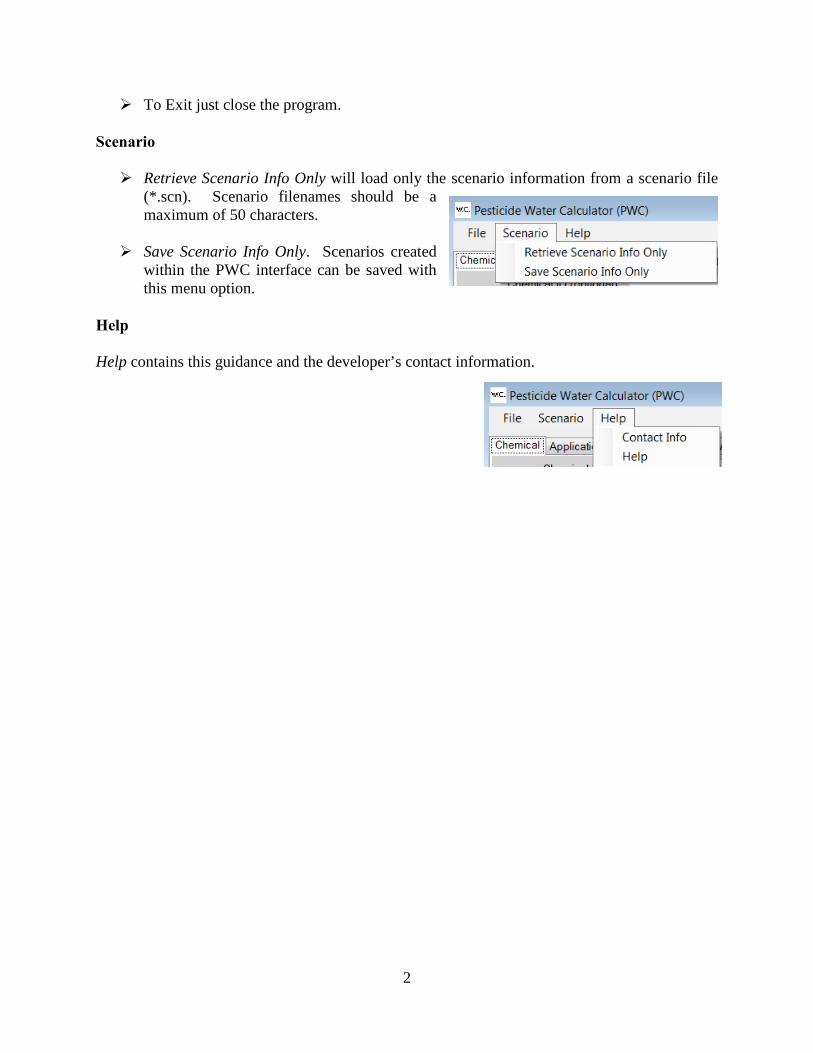
To Exit just close the program. Scenario Retrieve Scenario Info Only will load only the scenario information from a scenario file

(*.scn). Scenario filenames should be a maximum of 50 characters.

Save Scenario Info Only. Scenarios created

within the PWC interface can be saved with this menu option.

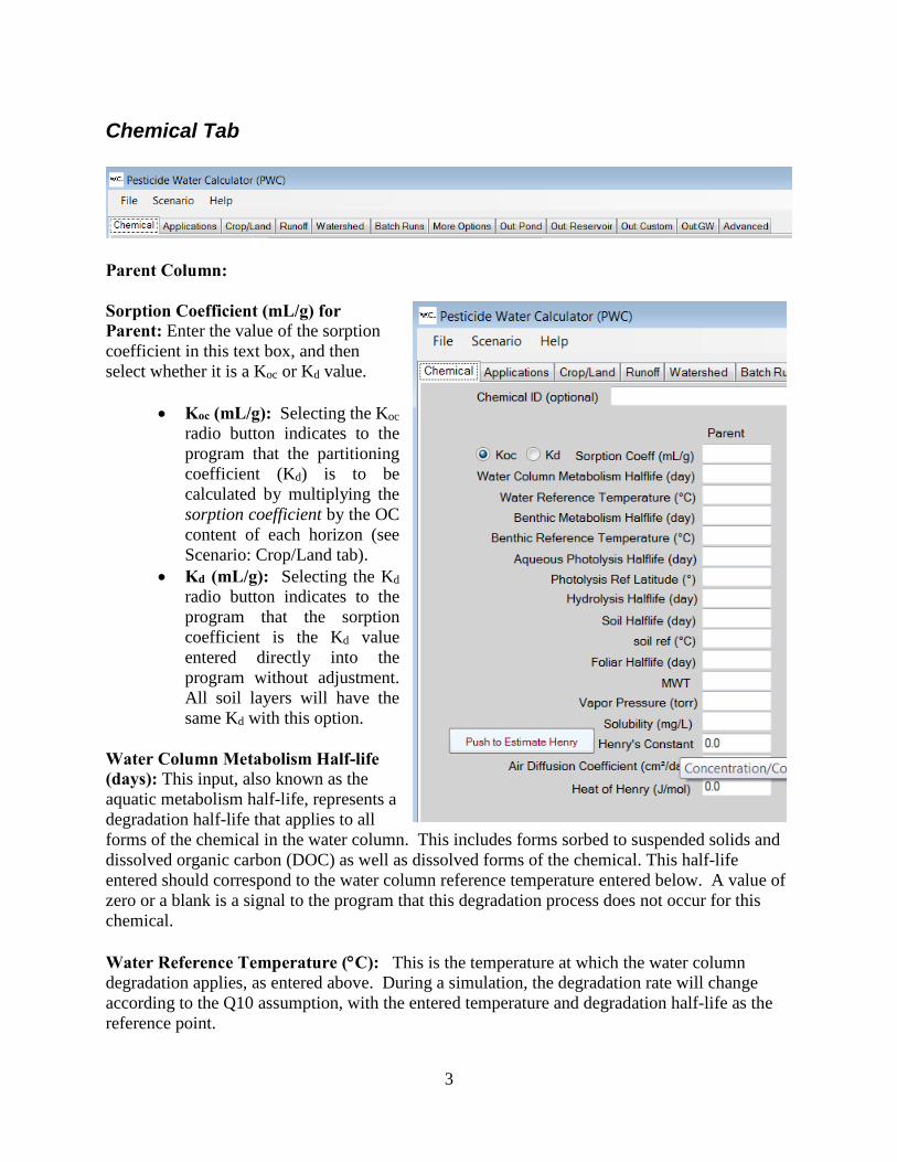
Help Help contains this guidance and the developer’s contact information.

3

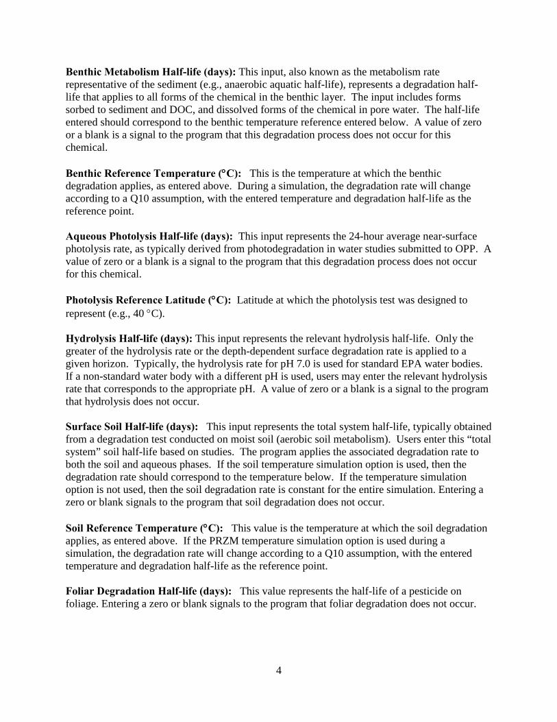
Chemical Tab

Parent Column: Sorption Coefficient (mL/g) for Parent: Enter the value of the sorption coefficient in this text box, and then select whether it is a Koc or Kd value.

• Koc (mL/g): Selecting the Koc radio button indicates to the program that the partitioning coefficient (Kd) is to be calculated by multiplying the sorption coefficient by the OC content of each horizon (see Scenario: Crop/Land tab).

• Kd (mL/g): Selecting the Kd radio button indicates to the program that the sorption coefficient is the Kd value entered directly into the program without adjustment. All soil layers will have the same Kd with this option.

Water Column Metabolism Half-life (days): This input, also known as the aquatic metabolism half-life, represents a degradation half-life that applies to all forms of the chemical in the water column. This includes forms sorbed to suspended solids and dissolved organic carbon (DOC) as well as dissolved forms of the chemical. This half-life entered should correspond to the water column reference temperature entered below. A value of zero or a blank is a signal to the program that this degradation process does not occur for this chemical. Water Reference Temperature (°C): This is the temperature at which the water column degradation applies, as entered above. During a simulation, the degradation rate will change according to the Q10 assumption, with the entered temperature and degradation half-life as the reference point.

4

Benthic Metabolism Half-life (days): This input, also known as the metabolism rate representative of the sediment (e.g., anaerobic aquatic half-life), represents a degradation half-life that applies to all forms of the chemical in the benthic layer. The input includes forms sorbed to sediment and DOC, and dissolved forms of the chemical in pore water. The half-life entered should correspond to the benthic temperature reference entered below. A value of zero or a blank is a signal to the program that this degradation process does not occur for this chemical. Benthic Reference Temperature (°C): This is the temperature at which the benthic degradation applies, as entered above. During a simulation, the degradation rate will change according to a Q10 assumption, with the entered temperature and degradation half-life as the reference point. Aqueous Photolysis Half-life (days): This input represents the 24-hour average near-surface photolysis rate, as typically derived from photodegradation in water studies submitted to OPP. A value of zero or a blank is a signal to the program that this degradation process does not occur for this chemical. Photolysis Reference Latitude (°C): Latitude at which the photolysis test was designed to represent (e.g., 40 °C). Hydrolysis Half-life (days): This input represents the relevant hydrolysis half-life. Only the greater of the hydrolysis rate or the depth-dependent surface degradation rate is applied to a given horizon. Typically, the hydrolysis rate for pH 7.0 is used for standard EPA water bodies. If a non-standard water body with a different pH is used, users may enter the relevant hydrolysis rate that corresponds to the appropriate pH. A value of zero or a blank is a signal to the program that hydrolysis does not occur. Surface Soil Half-life (days): This input represents the total system half-life, typically obtained from a degradation test conducted on moist soil (aerobic soil metabolism). Users enter this “total system” soil half-life based on studies. The program applies the associated degradation rate to both the soil and aqueous phases. If the soil temperature simulation option is used, then the degradation rate should correspond to the temperature below. If the temperature simulation option is not used, then the soil degradation rate is constant for the entire simulation. Entering a zero or blank signals to the program that soil degradation does not occur. Soil Reference Temperature (°C): This value is the temperature at which the soil degradation applies, as entered above. If the PRZM temperature simulation option is used during a simulation, the degradation rate will change according to a Q10 assumption, with the entered temperature and degradation half-life as the reference point. Foliar Degradation Half-life (days): This value represents the half-life of a pesticide on foliage. Entering a zero or blank signals to the program that foliar degradation does not occur.

5

MWT (g/mol): the molecular weight of the chemical. This value is used directly in the degradate production routines if degradates are simulated. It is also used indirectly to calculate the Henry’s Law coefficient.

NOTE: For volatilization routine refer to Guidance for Using the Volatilization Algorithm in the PWC and Water Exposure Models. Vapor Pressure (torr): vapor pressure of a pesticide at 25 °C. Used indirectly to calculate the Henry’s law coefficient. Solubility (mg/L): solubility of the pesticide in water at 25 °C. Used indirectly to calculate the Henry’s law coefficient. The program does not limit the concentration in water; solubility limit can be exceeded. Henry’s Constant (dimensionless): The dimensionless Henry’s Law Constant (Kh) is the partitioning coefficient of a chemical between air and moist soil. The graphical user interface enables the user to calculate Kh automatically from input vapor pressure and solubility values by clicking the “Push to Estimate Henry” button. The estimation routine assumes that the user entered vapor pressure and solubility relevant to 25°C . Air Diffusion Coefficient (cm2/day): used for volatilization routine. The air diffusion coefficient is related to the kinetic energy associated with molecular motion and is dependent on the molecular weight of the compound. An input of zero for the air diffusion coefficient effectively shuts off dissipation of the chemical due to volatilization. Heat of Henry (J/mol): This input is the enthalpy of phase change from aqueous solution to air solution (Joules/mole). This enthalpy can be approximated from the enthalpy of vaporization (Schwarzenbach et al., 1993), which can be obtained from EPISuite among other sources. Enthalpy for pesticides obtained in a literature review ranged from 20,000 to 100,000 J/mol (average 59,000 J/mol). Some example enthalpies for pesticides are Metalochlor 84,000 Feigenbrugel et al. 2004 Diazonon 98,000 Feigenbrugel et al. 2004 Alachlor 76,000 Gautier et al., 2003 Dichlorvos 95,000 Gautier et al., 2003

Mirex 91,000 Yin and Hassett, 1986 Lindane 43,000 Staudinger et al. (2000) EPTC 37,000 Staudinger et al. (2000) Molinate 58,000 Staudinger et al. (2000) Chlorpyrifos 17,000 Staudinger et al. (2000) Enthalpies can also be estimated by the US EPA EPI Suite software. Open the software, then select the HENRYWIN subprogram on the left of the EPI Suite screen. On the top menu of the HENRYWIN window item, select the ShowOptions, then select Show Temperature Variation

6

with Results. Enter the chemical name of interest and then push the Calculate button. EPI Suite will give the temperature variation results in the form of an equation: HLC (atm-m3/mole) = exp(A-(B/T)) {T in K}. The enthalpy of solvation in Joules/mol is equal to 8.314*B. Example enthalpies from EPI Suite are: Pendamethalin 62,000 J/mol Carbaryl 58,000 J/mol Carbofuran 54,000 J/mol Molinate 54,000 J/mol Endosulfan 37,000 J/mol Daughter Check Box Column: Checking this box allows for the simulation of a daughter degradate of the parent. Chemical properties of the degradate should be entered as described above for the parent. Granddaughter Check Box Column: This box is only available if the Daughter Check Box is checked. Checking this box allows for the simulation of a daughter degradate of degradate 1, or a second degradate of the parent (sequential reaction only). Chemical properties of this degradate should be entered as described above for the parent. Repeat the run for multiples degradates. Molar Conversion Factors: These values are the ratios of moles of degradate produced to moles of parent degraded for each of the processes. For example, if one parent molecule breaks down and produces one degradate then the ratio is 1. If the process does not produce the degradate of interest, then enter a zero.

NOTE: Ground Water Modeling In groundwater-modeling mode, water metabolism, benthic metabolism, and photolyisis are not used, and the respective text boxes do not need to be populated.

7

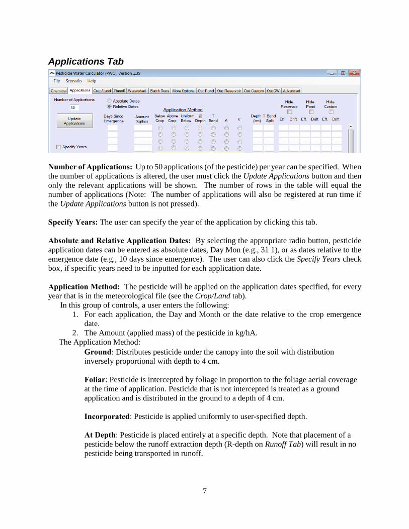
Applications Tab

Number of Applications: Up to 50 applications (of the pesticide) per year can be specified. When the number of applications is altered, the user must click the Update Applications button and then only the relevant applications will be shown. The number of rows in the table will equal the number of applications (Note: The number of applications will also be registered at run time if the Update Applications button is not pressed). Specify Years: The user can specify the year of the application by clicking this tab. Absolute and Relative Application Dates: By selecting the appropriate radio button, pesticide application dates can be entered as absolute dates, Day Mon (e.g., 31 1), or as dates relative to the emergence date (e.g., 10 days since emergence). The user can also click the Specify Years check box, if specific years need to be inputted for each application date. Application Method: The pesticide will be applied on the application dates specified, for every year that is in the meteorological file (see the Crop/Land tab).

In this group of controls, a user enters the following: 1. For each application, the Day and Month or the date relative to the crop emergence

date. 2. The Amount (applied mass) of the pesticide in kg/hA.

The Application Method: Ground: Distributes pesticide under the canopy into the soil with distribution inversely proportional with depth to 4 cm. Foliar: Pesticide is intercepted by foliage in proportion to the foliage aerial coverage at the time of application. Pesticide that is not intercepted is treated as a ground application and is distributed in the ground to a depth of 4 cm. Incorporated: Pesticide is applied uniformly to user-specified depth. At Depth: Pesticide is placed entirely at a specific depth. Note that placement of a pesticide below the runoff extraction depth (R-depth on Runoff Tab) will result in no pesticide being transported in runoff.

8

T-band: Pesticide is distributed to a depth specified by the incorporation depth, with a specified fraction (see T-Band Split below) placed into the top 2 cm. Δ. Pesticide mass is distributed in the soil linearly, increasing with depth down to the depth specified by the user.

∇ : Pesticide is distributed in the soil linearly, decreasing with depth down to the depth specified by the user.

Depth (cm): The depth of pesticide incorporations for the Incorporate, @Depth, and T-Band application methods (see above). T-Band Split: This is the fraction of the application rate that will be applied to the top 2 cm in a T-band application. Eff.: the efficiency, which is a multiplier of the application rate in PRZM. It is used to reduce the actual applied mass to the field, without changing the input application rate (has utility when performing spray drift applications). It does not affect the spray drift calculations. Typically, the efficiency is 0.95 for aerial spray and 0.99 for ground spray and orchard air blast. Drift/T: The spray drift fraction is used to calculate drift loading. It can also be used in a T-Band application to specify the fraction of the applied chemical incorporated into the top 2 cm. Typically for aquatic ecological exposure assessments (pond), use 0.05 for aerial spray, 0.01 for ground spray, or 0.03 for orchard air blast. In drinking water assessments (Reservoir), use 0.16 for aerial spray, 0.064 for ground spray, or 0.063 for orchard air blast. Refer to the Input Parameter Guidance for more information (USEPA, 2009)1 Custom, Reservoir, or Pond: User may select any of these three options, based on the simulation type being performed. Note that the Eff. and Drift/T need to be filled accordingly if more than one water body is used. Application Refinements: These options allow flexibility in how the applications occur.

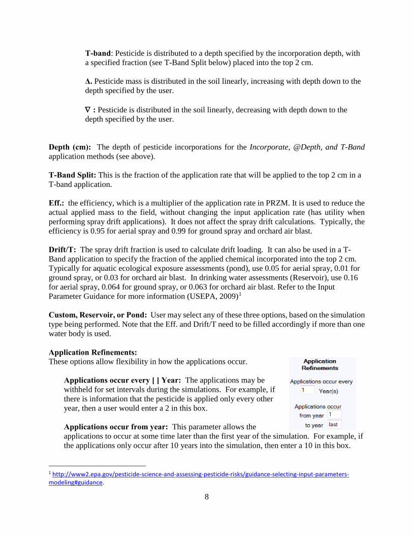
Applications occur every [ ] Year: The applications may be withheld for set intervals during the simulations. For example, if there is information that the pesticide is applied only every other year, then a user would enter a 2 in this box. Applications occur from year: This parameter allows the applications to occur at some time later than the first year of the simulation. For example, if the applications only occur after 10 years into the simulation, then enter a 10 in this box.

1 http://www2.epa.gov/pesticide-science-and-assessing-pesticide-risks/guidance-selecting-input-parameters-modeling#guidance.

9

Applications occur to year: This parameter allows the applications to end at some time prior to the last year of the simulation. For example, if the applications only occur for the first 15 years and then stop, enter a 15 in this box.

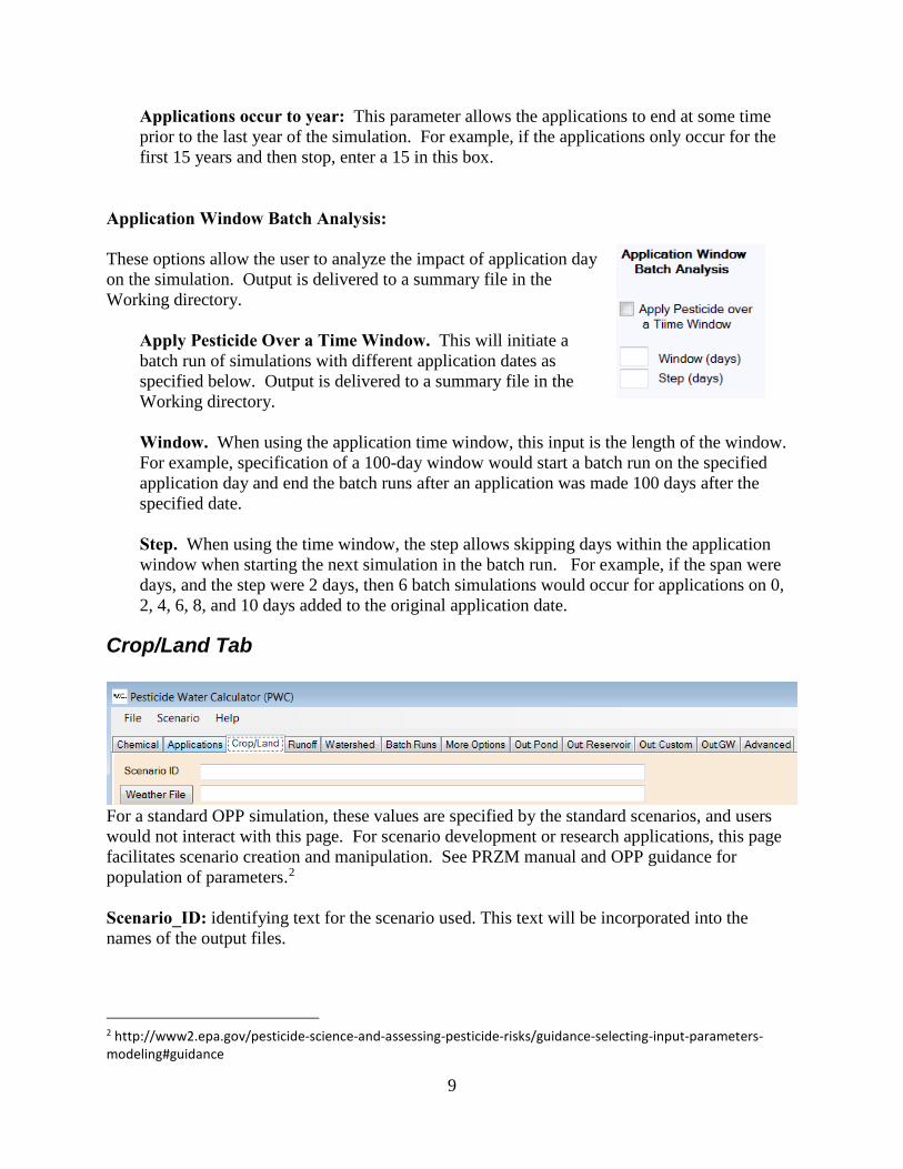
Application Window Batch Analysis: These options allow the user to analyze the impact of application day on the simulation. Output is delivered to a summary file in the Working directory.

Apply Pesticide Over a Time Window. This will initiate a batch run of simulations with different application dates as specified below. Output is delivered to a summary file in the Working directory. Window. When using the application time window, this input is the length of the window. For example, specification of a 100-day window would start a batch run on the specified application day and end the batch runs after an application was made 100 days after the specified date. Step. When using the time window, the step allows skipping days within the application window when starting the next simulation in the batch run. For example, if the span were days, and the step were 2 days, then 6 batch simulations would occur for applications on 0, 2, 4, 6, 8, and 10 days added to the original application date.

Crop/Land Tab

For a standard OPP simulation, these values are specified by the standard scenarios, and users would not interact with this page. For scenario development or research applications, this page facilitates scenario creation and manipulation. See PRZM manual and OPP guidance for population of parameters.2 Scenario_ID: identifying text for the scenario used. This text will be incorporated into the names of the output files.

2 http://www2.epa.gov/pesticide-science-and-assessing-pesticide-risks/guidance-selecting-input-parameters-modeling#guidance

10

Weather File button opens a file browser to allow for selection of weather files. Files must be in the same format as PRZM weather files.

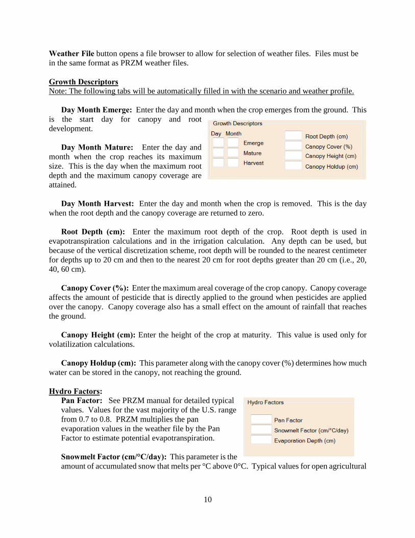
Growth Descriptors Note: The following tabs will be automatically filled in with the scenario and weather profile.

Day Month Emerge: Enter the day and month when the crop emerges from the ground. This

is the start day for canopy and root development.

Day Month Mature: Enter the day and

month when the crop reaches its maximum size. This is the day when the maximum root depth and the maximum canopy coverage are attained.

Day Month Harvest: Enter the day and month when the crop is removed. This is the day

when the root depth and the canopy coverage are returned to zero.

Root Depth (cm): Enter the maximum root depth of the crop. Root depth is used in evapotranspiration calculations and in the irrigation calculation. Any depth can be used, but because of the vertical discretization scheme, root depth will be rounded to the nearest centimeter for depths up to 20 cm and then to the nearest 20 cm for root depths greater than 20 cm (i.e., 20, 40, 60 cm).

Canopy Cover (%): Enter the maximum areal coverage of the crop canopy. Canopy coverage affects the amount of pesticide that is directly applied to the ground when pesticides are applied over the canopy. Canopy coverage also has a small effect on the amount of rainfall that reaches the ground.

Canopy Height (cm): Enter the height of the crop at maturity. This value is used only for

volatilization calculations. Canopy Holdup (cm): This parameter along with the canopy cover (%) determines how much

water can be stored in the canopy, not reaching the ground.

Hydro Factors: Pan Factor: See PRZM manual for detailed typical values. Values for the vast majority of the U.S. range from 0.7 to 0.8. PRZM multiplies the pan evaporation values in the weather file by the Pan Factor to estimate potential evapotranspiration. Snowmelt Factor (cm/°C/day): This parameter is the amount of accumulated snow that melts per °C above 0°C. Typical values for open agricultural

11

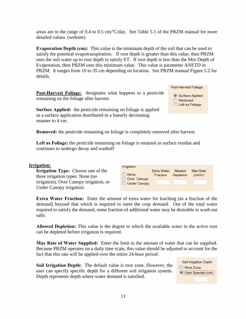
areas are in the range of 0.4 to 0.5 cm/oC/day. See Table 5.1 of the PRZM manual for more detailed values. (website) Evaporation Depth (cm): This value is the minimum depth of the soil that can be used to satisfy the potential evapotranspiration. If root depth is greater than this value, then PRZM uses the soil water up to root depth to satisfy ET. If root depth is less than the Min Depth of Evaporation, then PRZM uses this minimum value. This value is parameter ANETD in PRZM. It ranges from 10 to 35 cm depending on location. See PRZM manual Figure 5.2 for details. Post-Harvest Foliage: designates what happens to a pesticide remaining on the foliage after harvest. Surface Applied: the pesticide remaining on foliage is applied as a surface application distributed in a linearly decreasing manner to 4 cm.

Removed: the pesticide remaining on foliage is completely removed after harvest.

Left as Foliage: the pesticide remaining on foliage is retained as surface residue and continues to undergo decay and washoff

Irrigation:

Irrigation Type: Choose one of the three irrigation types: None (no irrigation), Over Canopy irrigation, or Under Canopy irrigation.

Extra Water Fraction: Enter the amount of extra water for leaching (as a fraction of the demand) beyond that which is required to meet the crop demand. Out of the total water required to satisfy the demand, some fraction of additional water may be desirable to wash out salts. Allowed Depletion: This value is the degree to which the available water in the active root can be depleted before irrigation is required. Max Rate of Water Supplied: Enter the limit to the amount of water that can be supplied. Because PRZM operates on a daily time scale, this value should be adjusted to account for the fact that this rate will be applied over the entire 24-hour period.

Soil Irrigation Depth: The default value is root zone. However, the user can specify specific depth for a different soil irrigation system. Depth represents depth where water demand is satisfied.

12

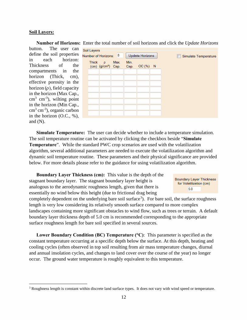
Soil Layers: Number of Horizons: Enter the total number of soil horizons and click the Update Horizons button. The user can define the soil properties in each horizon: Thickness of the compartments in the horizon (Thick, cm), effective porosity in the horizon (ρ), field capacity in the horizon (Max Cap., cm3 cm-3), wilting point in the horizon (Min Cap., cm3 cm-3), organic carbon in the horizon (O.C., %), and (N). Simulate Temperature: The user can decide whether to include a temperature simulation. The soil temperature routine can be activated by clicking the checkbox beside “Simulate Temperature”. While the standard PWC crop scenarios are used with the volatilization algorithm, several additional parameters are needed to execute the volatilization algorithm and dynamic soil temperature routine. These parameters and their physical significance are provided below. For more details please refer to the guidance for using volatilization algorithm.

Boundary Layer Thickness (cm): This value is the depth of the stagnant boundary layer. The stagnant boundary layer height is analogous to the aerodynamic roughness length, given that there is essentially no wind below this height (due to frictional drag being completely dependent on the underlying bare soil surface3). For bare soil, the surface roughness length is very low considering its relatively smooth surface compared to more complex landscapes containing more significant obstacles to wind flow, such as trees or terrain. A default boundary layer thickness depth of 5.0 cm is recommended corresponding to the appropriate surface roughness length for bare soil specified in several sources.

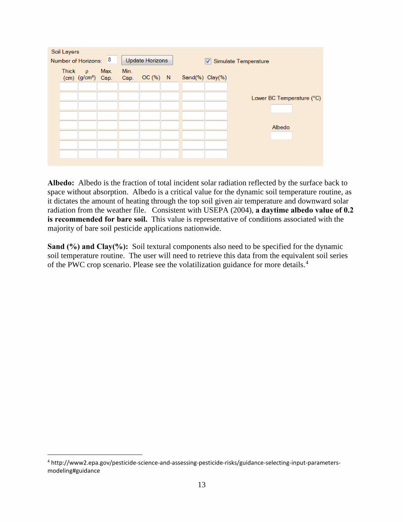
Lower Boundary Condition (BC) Temperature (°C): This parameter is specified as the

constant temperature occurring at a specific depth below the surface. At this depth, heating and cooling cycles (often observed in top soil resulting from air mass temperature changes, diurnal and annual insolation cycles, and changes to land cover over the course of the year) no longer occur. The ground water temperature is roughly equivalent to this temperature.

3 Roughness length is constant within discrete land surface types. It does not vary with wind speed or temperature.

13

Albedo: Albedo is the fraction of total incident solar radiation reflected by the surface back to space without absorption. Albedo is a critical value for the dynamic soil temperature routine, as it dictates the amount of heating through the top soil given air temperature and downward solar radiation from the weather file. Consistent with USEPA (2004), a daytime albedo value of 0.2 is recommended for bare soil. This value is representative of conditions associated with the majority of bare soil pesticide applications nationwide. Sand (%) and Clay(%): Soil textural components also need to be specified for the dynamic soil temperature routine. The user will need to retrieve this data from the equivalent soil series of the PWC crop scenario. Please see the volatilization guidance for more details.4

4 http://www2.epa.gov/pesticide-science-and-assessing-pesticide-risks/guidance-selecting-input-parameters-modeling#guidance

14

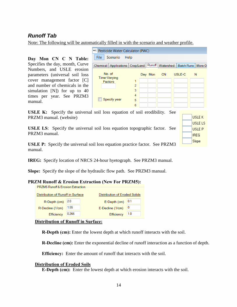
Runoff Tab Note: The following will be automatically filled in with the scenario and weather profile. Day Mon CN C N Table: Specifies the day, month, Curve Numbers, and USLE erosion parameters (universal soil loss cover management factor [C] and number of chemicals in the simulation [N]) for up to 40 times per year. See PRZM3 manual. USLE K: Specify the universal soil loss equation of soil erodibility. See PRZM3 manual. (website)

USLE LS: Specify the universal soil loss equation topographic factor. See PRZM3 manual.

USLE P: Specify the universal soil loss equation practice factor. See PRZM3 manual.

IREG: Specify location of NRCS 24-hour hyetograph. See PRZM3 manual.

Slope: Specify the slope of the hydraulic flow path. See PRZM3 manual. PRZM Runoff & Erosion Extraction (New For PRZM5):

Distribution of Runoff in Surface:

R-Depth (cm): Enter the lowest depth at which runoff interacts with the soil.

R-Decline (cm): Enter the exponential decline of runoff interaction as a function of depth.

Efficiency: Enter the amount of runoff that interacts with the soil.

Distribution of Eroded Soils

E-Depth (cm): Enter the lowest depth at which erosion interacts with the soil.

15

E-Decline (1/cm): Enter the exponential decline of erosion interaction as a function of depth. Efficiency: The contribution of the eroded soil in runoff. Enter the fraction of the eroded soil that interacts with the surface for removal of pesticide.

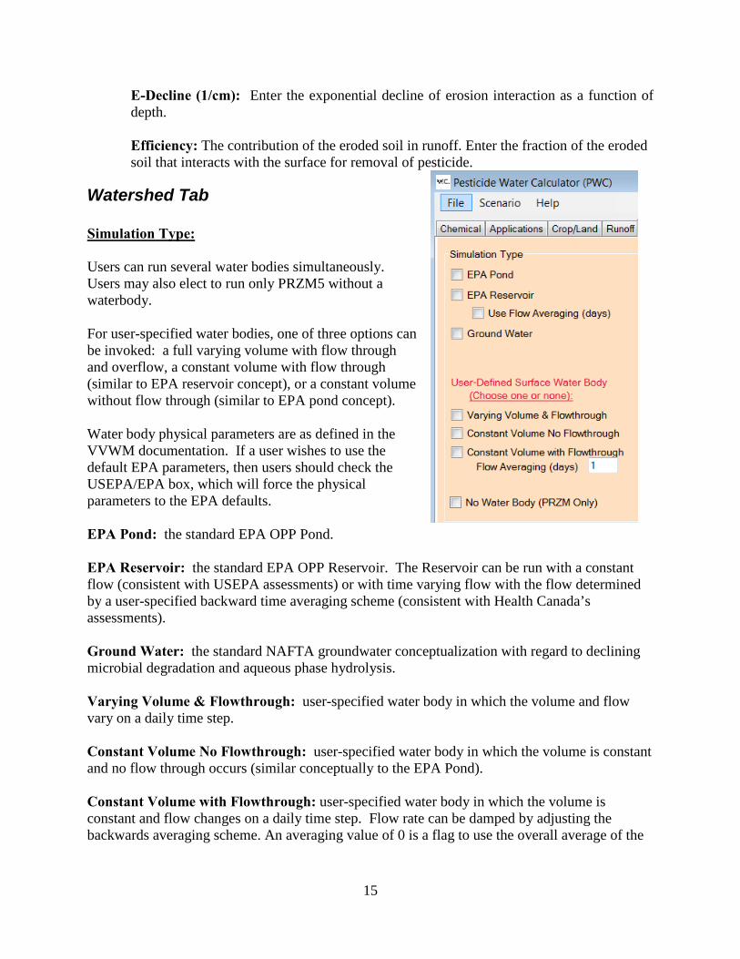
Watershed Tab Simulation Type: Users can run several water bodies simultaneously. Users may also elect to run only PRZM5 without a waterbody. For user-specified water bodies, one of three options can be invoked: a full varying volume with flow through and overflow, a constant volume with flow through (similar to EPA reservoir concept), or a constant volume without flow through (similar to EPA pond concept). Water body physical parameters are as defined in the VVWM documentation. If a user wishes to use the default EPA parameters, then users should check the USEPA/EPA box, which will force the physical parameters to the EPA defaults. EPA Pond: the standard EPA OPP Pond. EPA Reservoir: the standard EPA OPP Reservoir. The Reservoir can be run with a constant flow (consistent with USEPA assessments) or with time varying flow with the flow determined by a user-specified backward time averaging scheme (consistent with Health Canada’s assessments). Ground Water: the standard NAFTA groundwater conceptualization with regard to declining microbial degradation and aqueous phase hydrolysis. Varying Volume & Flowthrough: user-specified water body in which the volume and flow vary on a daily time step. Constant Volume No Flowthrough: user-specified water body in which the volume is constant and no flow through occurs (similar conceptually to the EPA Pond). Constant Volume with Flowthrough: user-specified water body in which the volume is constant and flow changes on a daily time step. Flow rate can be damped by adjusting the backwards averaging scheme. An averaging value of 0 is a flag to use the overall average of the

16

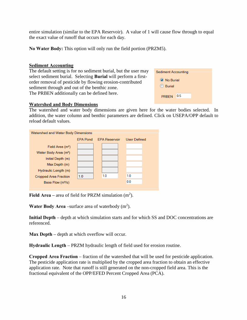
entire simulation (similar to the EPA Reservoir). A value of 1 will cause flow through to equal the exact value of runoff that occurs for each day. No Water Body: This option will only run the field portion (PRZM5). Sediment Accounting The default setting is for no sediment burial, but the user may select sediment burial. Selecting Burial will perform a first-order removal of pesticide by flowing erosion-contributed sediment through and out of the benthic zone. The PRBEN additionally can be defined here. Watershed and Body Dimensions The watershed and water body dimensions are given here for the water bodies selected. In addition, the water column and benthic parameters are defined. Click on USEPA/OPP default to reload default values.

Field Area – area of field for PRZM simulation (m2). Water Body Area –surface area of waterbody (m2). Initial Depth – depth at which simulation starts and for which SS and DOC concentrations are referenced. Max Depth – depth at which overflow will occur. Hydraulic Length – PRZM hydraulic length of field used for erosion routine. Cropped Area Fraction – fraction of the watershed that will be used for pesticide application. The pesticide application rate is multiplied by the cropped area fraction to obtain an effective application rate. Note that runoff is still generated on the non-cropped field area. This is the fractional equivalent of the OPP/EFED Percent Cropped Area (PCA).

17

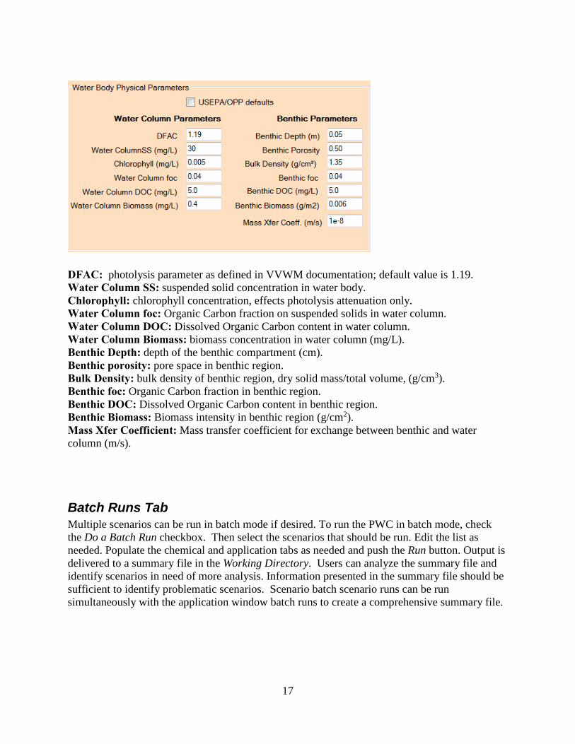
DFAC: photolysis parameter as defined in VVWM documentation; default value is 1.19. Water Column SS: suspended solid concentration in water body. Chlorophyll: chlorophyll concentration, effects photolysis attenuation only. Water Column foc: Organic Carbon fraction on suspended solids in water column. Water Column DOC: Dissolved Organic Carbon content in water column. Water Column Biomass: biomass concentration in water column (mg/L). Benthic Depth: depth of the benthic compartment (cm). Benthic porosity: pore space in benthic region. Bulk Density: bulk density of benthic region, dry solid mass/total volume, (g/cm3). Benthic foc: Organic Carbon fraction in benthic region. Benthic DOC: Dissolved Organic Carbon content in benthic region. Benthic Biomass: Biomass intensity in benthic region (g/cm2). Mass Xfer Coefficient: Mass transfer coefficient for exchange between benthic and water column (m/s).

Batch Runs Tab Multiple scenarios can be run in batch mode if desired. To run the PWC in batch mode, check the Do a Batch Run checkbox. Then select the scenarios that should be run. Edit the list as needed. Populate the chemical and application tabs as needed and push the Run button. Output is delivered to a summary file in the Working Directory. Users can analyze the summary file and identify scenarios in need of more analysis. Information presented in the summary file should be sufficient to identify problematic scenarios. Scenario batch scenario runs can be run simultaneously with the application window batch runs to create a comprehensive summary file.

18

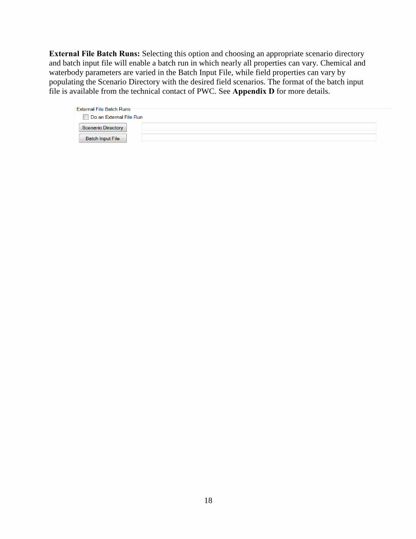
External File Batch Runs: Selecting this option and choosing an appropriate scenario directory and batch input file will enable a batch run in which nearly all properties can vary. Chemical and waterbody parameters are varied in the Batch Input File, while field properties can vary by populating the Scenario Directory with the desired field scenarios. The format of the batch input file is available from the technical contact of PWC. See Appendix D for more details.

19

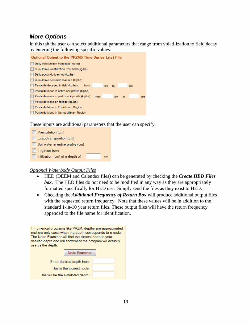
More Options In this tab the user can select additional parameters that range from volatilization to field decay by entering the following specific values:

These inputs are additional parameters that the user can specify:

Optional Waterbody Output Files

• HED (DEEM and Calendex files) can be generated by checking the Create HED Files box. The HED files do not need to be modified in any way as they are appropriately formatted specifically for HED use. Simply send the files as they exist to HED.

• Checking the Additional Frequency of Return Box will produce additional output files with the requested return frequency. Note that these values will be in addition to the standard 1-in-10 year return files. These output files will have the return frequency appended to the file name for identification.

20

Out:Pond Tab This output tab gives results for the USEPA Pond.

Out:Reservoir Tab This output tab gives results for the USEPA Drinking Water Reservoir.

Out:Custom Tab This output tab gives results for the user-defined water body.

The graphs on these three output tabs show annual peaks for the water column and benthic pore water.

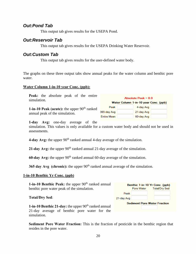
Water Column 1-in-10 year Conc. (ppb):

Peak: the absolute peak of the entire simulation. 1-in-10 Peak (acute): the upper 90th ranked annual peak of the simulation. 1-day Avg: one-day average of the simulation. This values is only available for a custom water body and should not be used in assessments. 4-day Avg: the upper 90th ranked annual 4-day average of the simulation. 21-day Avg: the upper 90th ranked annual 21-day average of the simulation. 60-day Avg: the upper 90th ranked annual 60-day average of the simulation.

365 day Avg (chronic): the upper 90th ranked annual average of the simulation.

1-in-10 Benthic Yr Conc. (ppb) 1-in-10 Benthic Peak: the upper 90th ranked annual benthic pore water peak of the simulation. Total/Dry Sed: 1-in-10 Benthic 21-day: the upper 90th ranked annual 21-day average of benthic pore water for the simulation. Sediment Pore Water Fraction: This is the fraction of pesticide in the benthic region that resides in the pore water.

21

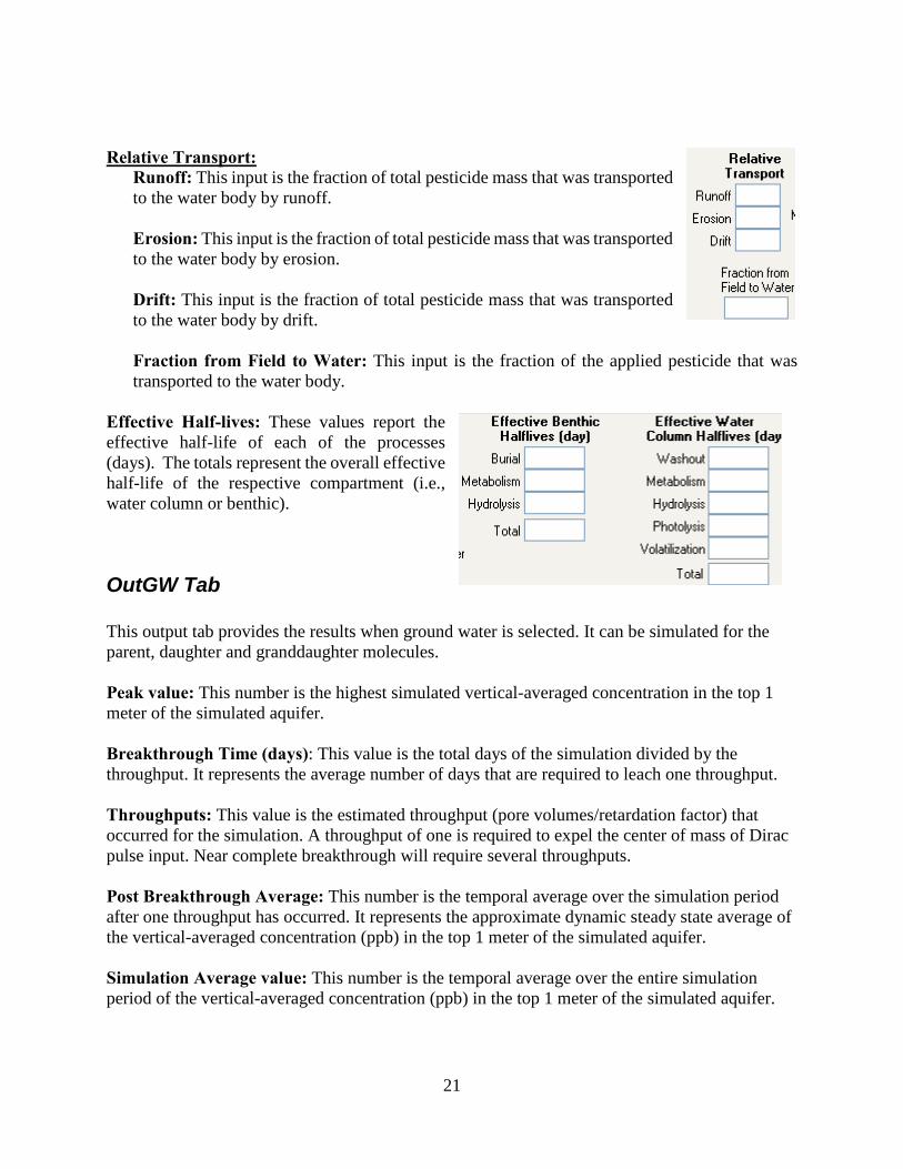
Relative Transport:

Runoff: This input is the fraction of total pesticide mass that was transported to the water body by runoff.

Erosion: This input is the fraction of total pesticide mass that was transported to the water body by erosion.

Drift: This input is the fraction of total pesticide mass that was transported to the water body by drift.

Fraction from Field to Water: This input is the fraction of the applied pesticide that was transported to the water body.

Effective Half-lives: These values report the effective half-life of each of the processes (days). The totals represent the overall effective half-life of the respective compartment (i.e., water column or benthic).

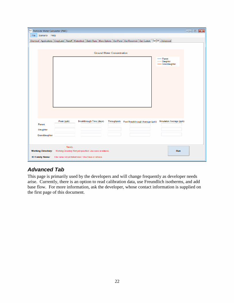
OutGW Tab This output tab provides the results when ground water is selected. It can be simulated for the parent, daughter and granddaughter molecules. Peak value: This number is the highest simulated vertical-averaged concentration in the top 1 meter of the simulated aquifer. Breakthrough Time (days): This value is the total days of the simulation divided by the throughput. It represents the average number of days that are required to leach one throughput. Throughputs: This value is the estimated throughput (pore volumes/retardation factor) that occurred for the simulation. A throughput of one is required to expel the center of mass of Dirac pulse input. Near complete breakthrough will require several throughputs. Post Breakthrough Average: This number is the temporal average over the simulation period after one throughput has occurred. It represents the approximate dynamic steady state average of the vertical-averaged concentration (ppb) in the top 1 meter of the simulated aquifer. Simulation Average value: This number is the temporal average over the entire simulation period of the vertical-averaged concentration (ppb) in the top 1 meter of the simulated aquifer.

22

Advanced Tab This page is primarily used by the developers and will change frequently as developer needs arise. Currently, there is an option to read calibration data, use Freundlich isotherms, and add base flow. For more information, ask the developer, whose contact information is supplied on the first page of this document.

23

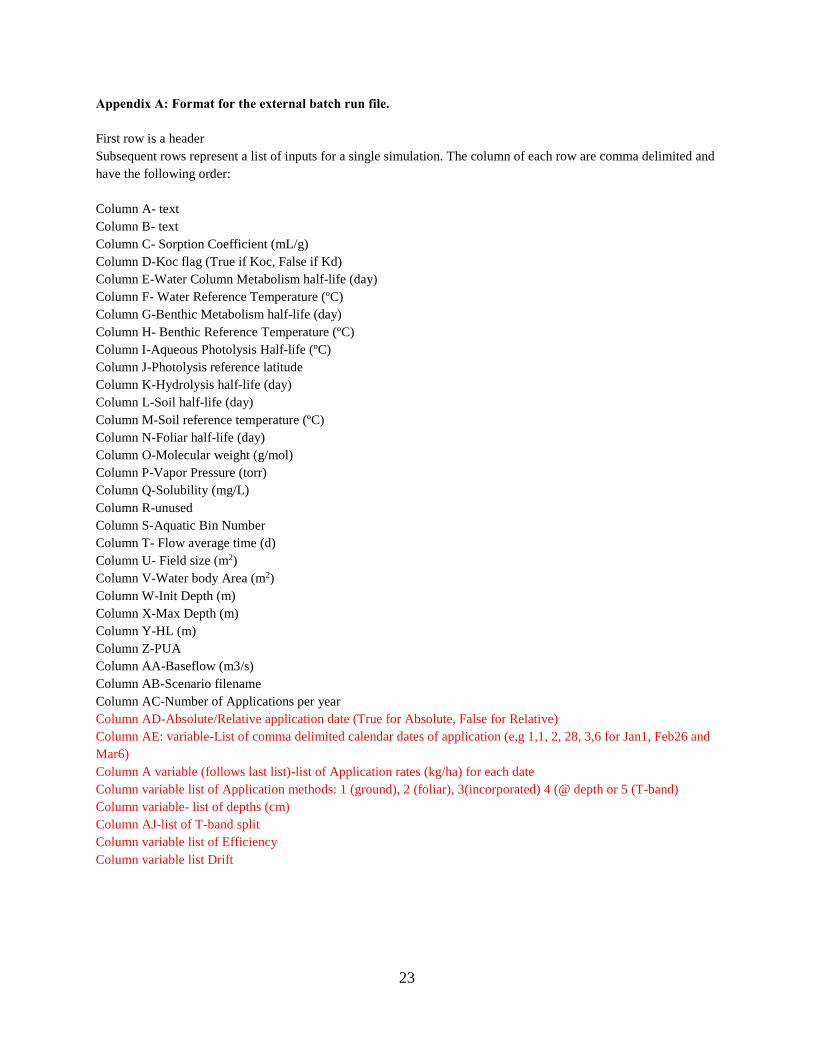
Appendix A: Format for the external batch run file. First row is a header Subsequent rows represent a list of inputs for a single simulation. The column of each row are comma delimited and have the following order: Column A- text Column B- text Column C- Sorption Coefficient (mL/g) Column D-Koc flag (True if Koc, False if Kd) Column E-Water Column Metabolism half-life (day) Column F- Water Reference Temperature (ºC) Column G-Benthic Metabolism half-life (day) Column H- Benthic Reference Temperature (ºC) Column I-Aqueous Photolysis Half-life (ºC) Column J-Photolysis reference latitude Column K-Hydrolysis half-life (day) Column L-Soil half-life (day) Column M-Soil reference temperature (ºC) Column N-Foliar half-life (day) Column O-Molecular weight (g/mol) Column P-Vapor Pressure (torr) Column Q-Solubility (mg/L) Column R-unused Column S-Aquatic Bin Number Column T- Flow average time (d) Column U- Field size (m2) Column V-Water body Area (m2) Column W-Init Depth (m) Column X-Max Depth (m) Column Y-HL (m) Column Z-PUA Column AA-Baseflow (m3/s) Column AB-Scenario filename Column AC-Number of Applications per year Column AD-Absolute/Relative application date (True for Absolute, False for Relative) Column AE: variable-List of comma delimited calendar dates of application (e,g 1,1, 2, 28, 3,6 for Jan1, Feb26 and Mar6) Column A variable (follows last list)-list of Application rates (kg/ha) for each date Column variable list of Application methods: 1 (ground), 2 (foliar), 3(incorporated) 4 (@ depth or 5 (T-band) Column variable- list of depths (cm) Column AJ-list of T-band split Column variable list of Efficiency Column variable list Drift