Embed Size (px)
Citation preview

Perturbation and Projection Methods for Solving DSGE Models
Lawrence J. Christiano
Discussion of projections taken from Christiano‐Fisher, ‘Algorithms for Solving Dynamic Models with Occasionally Binding Constraints’, 2000, Journal of Economic Dynamics and Control.Discussion of perturbations taken from Judd’s textbook.
Outline• A Toy Example to Illustrate the basic ideas.
– Functional form characterization of model solution.
– Use of Projections and Perturbations.
• Neoclassical model.– Projection methods– Perturbation methods
• Make sense of the proposition, ‘to a first order approximation, can replace equilibrium conditions with linear expansion about nonstochastic steady state and solve the resulting system using certainty equivalence’
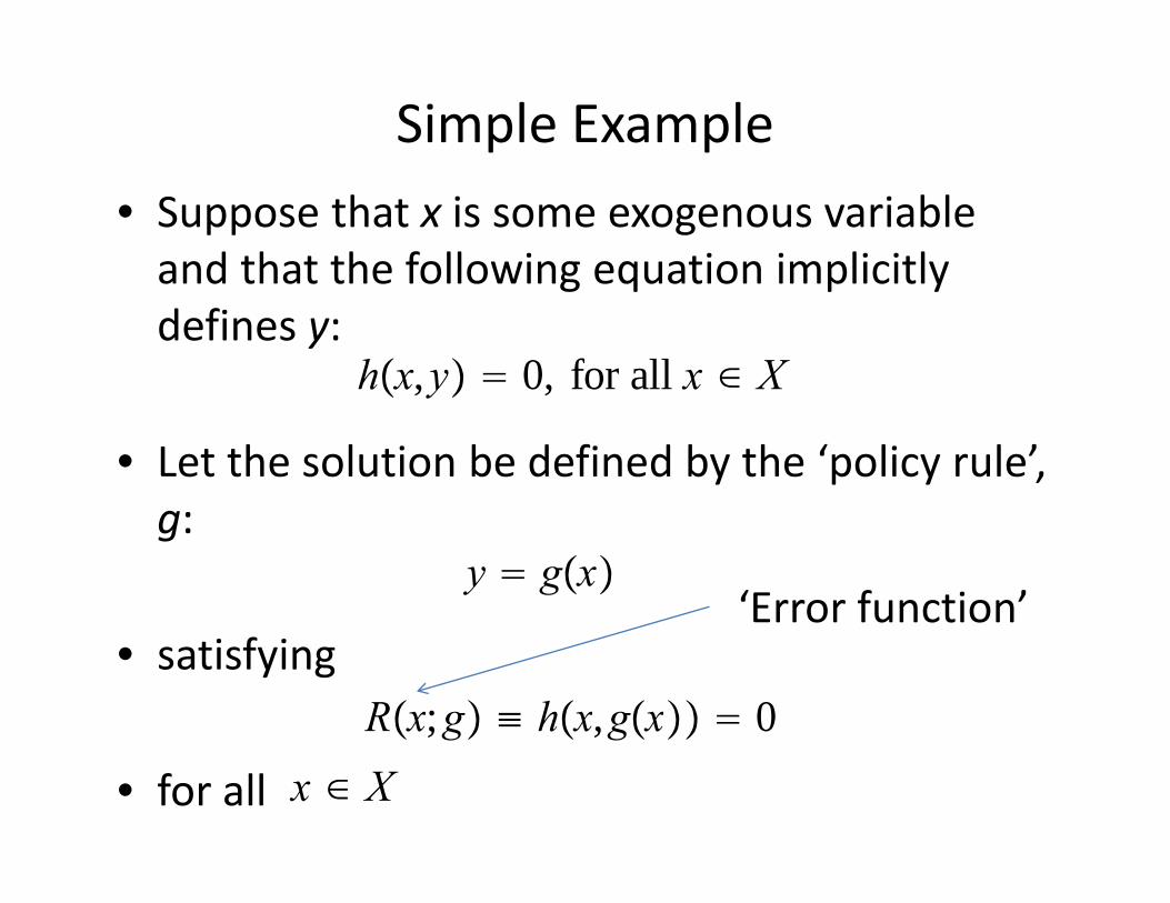
Simple Example• Suppose that x is some exogenous variable and that the following equation implicitly defines y:
• Let the solution be defined by the ‘policy rule’, g:
• satisfying
• for all
Rx;g ≡ hx,gx 0
y gx
hx,y 0, for all x ∈ X
x ∈ X
‘Error function’

The Need to Approximate• Finding the policy rule, g, is a big problem outside special cases
– ‘Infinite number of unknowns (i.e., one value of gfor each possible x) in an infinite number of equations (i.e., one equation for each possible x).’
• Two approaches:
– projection and perturbation
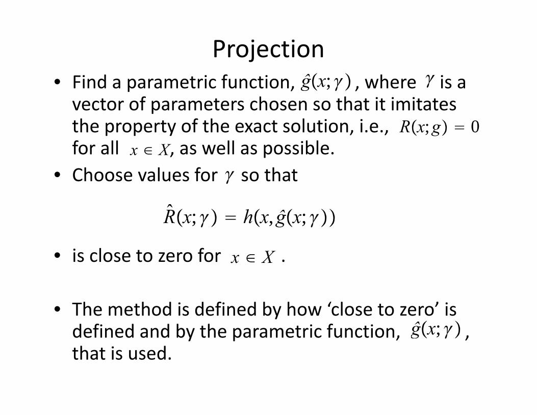
Projection• Find a parametric function, , where is a vector of parameters chosen so that it imitates the property of the exact solution, i.e., for all , as well as possible.
• Choose values for so that
• is close to zero for .
• The method is defined by how ‘close to zero’ is defined and by the parametric function, , that is used.
ĝx;
R̂x; hx,ĝx;
ĝx;
Rx;g 0x ∈ X
x ∈ X

Projection, continued• Spectral and finite element approximations
– Spectral functions: functions, , in which each parameter in influences for all example:
ĝx; ĝx; x ∈ X
ĝx; ∑i0
n
iHix, 1
n
Hix xi ~ordinary polynominal (not computationaly efficient)Hix Tix,Tiz : −1,1 → −1,1, ith order Chebyshev polynomial
: X → −1,1
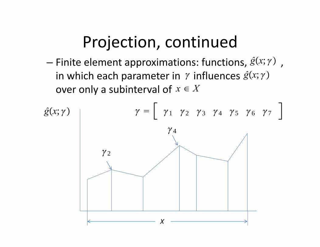
Projection, continued– Finite element approximations: functions, , in which each parameter in influences over only a subinterval of
ĝx; ĝx;
x ∈ X
X
ĝx;
4
2
1 2 3 4 5 6 7

Projection, continued • ‘Close to zero’: two methods• Collocation, for n values of choose n elements of so that
– how you choose the grid of x’s matters…
• Weighted Residual, for m>n values of xxxxxxxx choose the n
x : x1,x2, . . . ,xn ∈ X
R̂xi; hxi,ĝxi; 0, i 1, . . . ,n
1 n
∑j1
m
wjihxj,ĝxj; 0, i 1, . . . ,n
i’sx : x1,x2, . . . ,xm ∈ X

Example of Importance of Grid Points• Here is an example, taken from a related problem, the problem
of interpolation.– You get to evaluate a function on a set of grid points that you select, and you must guess the shape of the function between the grid points.
• Consider the function,
• Next slide shows what happens when you select 11 equally‐spaced grid points and interpolate by fitting a 10th order polynomial. – As you increase the number of grid points on a fixed interval grid, oscillations in tails grow more and more violent.
• Chebyshev approximation theorem: distribute more points in the tails (by selecting zeros of Chebyshev polynomial) and get convergence in sup norm.
fk 11 k2 , k ∈ −5,5

How You Select the Grid Points Matters
Figure from Christiano‐Fisher, JEDC, 1990


Projection, continued • ‘Close to zero’: two methods• Collocation, for n values of choose n elements of so that
– how you choose the grid of x’s matters…
• Weighted Residual, for m>n values of xxxxxxxx choose the n
x : x1,x2, . . . ,xn ∈ X
R̂xi; hxi,ĝxi; 0, i 1, . . . ,n
1 n
∑j1
m
wjihxj,ĝxj; 0, i 1, . . . ,n
i’sx : x1,x2, . . . ,xm ∈ X

Perturbation• Projection uses the ‘global’ behavior of the functional equation to approximate solution.– Problem: requires finding zeros of non‐linear equations. Iterative methods for doing this are a pain.
– Advantage: can easily adapt to situations the policy rule is not continuous or simply non‐differentiable (e.g., occasionally binding zero lower bound on interest rate).
• Perturbation method uses local properties of functional equation and Implicit Function/Taylor’s theorem to approximate solution.– Advantage: can implement it using non‐iterative methods. – Possible disadvantages:
• may require enormously high derivatives to achieve a decent global approximation.
• Does not work when there are important non‐differentiabilities(e.g., occasionally binding zero lower bound on interest rate).

Perturbation, cnt’d• Suppose there is a point, , where we know the value taken on by the function, g, that we wish to approximate:
• Use the implicit function theorem to approximate g in a neighborhood of
• Note:
x∗ ∈ X
Rx;g 0 for all x ∈ X→
Rjx;g ≡ djdxjRx;g 0 for all j, all x ∈ X.
gx∗ g∗, some x∗
x∗

Perturbation, cnt’d• Differentiate R with respect to and evaluate the result at :
• Do it again!
R1x∗ ddx hx,gx|xx
∗ h1x∗,g∗ h2x∗,g∗g′x∗ 0
→ g′x∗ − h1x∗,g∗h2x∗,g∗
xx∗
R2x∗ d2
dx2 hx,gx|xx∗ h11x∗,g∗ 2h12x∗,g∗g′x∗
h22x∗,g∗g′x∗2 h2x∗,g∗g′′x∗.
→ Solve this linearly for g′′x∗.

Perturbation, cnt’d• Preceding calculations deliver (assuming enough differentiability, appropriate invertibility, a high tolerance for painful notation!), recursively:
• Then, have the following Taylor’s series approximation:
g′x∗ ,g′′x∗ , . . . ,gnx∗
gx ≈ ĝxĝx g∗ g′x∗ x − x∗
12 g
′′x∗ x − x∗ 2 . . . 1n! g
nx∗ x − x∗n

Perturbation, cnt’d
• Check….• Study the graph of
– over to verify that it is everywhere close to zero (or, at least in the region of interest).
Rx;ĝ
x ∈ X

Example of Implicit Function Theoremhx,y 1
2 x2 y2 − 8 0
x
y
4
4
‐4
‐4
g′x∗ − h1x∗,g∗h2x∗,g∗
− x∗
g∗ h2 had better not be zero!
gx ≃ g∗ − x∗
g∗ x − x∗

Neoclassical Growth Model
• Objective:
• Constraints:
E0∑t0
tuct, uct ct
1− − 11 −
ct expkt1 ≤ fkt,at, t 0,1,2, . . . .
at at−1 t, t~ Et 0, Et2 V
fkt,at expktexpat 1 − expkt
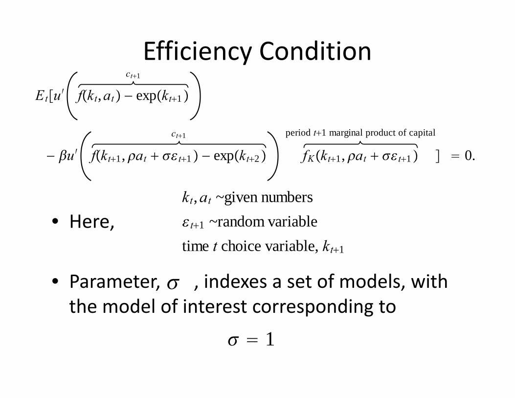
Efficiency Condition
• Here,
• Parameter, , indexes a set of models, with the model of interest corresponding to
Etu′ct1
fkt,at − expkt1
− u′ct1
fkt1,at t1 − expkt2
period t1 marginal product of capital
fKkt1,at t1 0.
kt,at ~given numberst1 ~random variabletime t choice variable, kt1
1
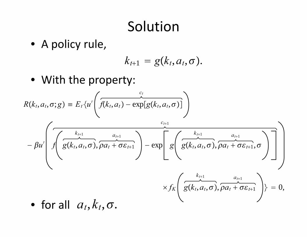
Solution• A policy rule,
• With the property:
• for all
kt1 gkt,at,.
Rkt,at,;g ≡ Etu′ct
fkt,at − expgkt,at,
− u′
ct1
fkt1
gkt,at,,at1
at t1 − exp gkt1
gkt,at,,at1
at t1,
fK
kt1
gkt,at,,at1
at t1 0,
at,kt,.

Projection Methods• Let
– be a function with finite parameters (could be either spectral or finite element, as before).
• Choose parameters, , to make
– as close to zero as possible, over a range of values of the state.
– use weighted residuals or Collocation.
ĝkt,at,;
Rkt,at,;ĝ

Occasionally Binding Constraints• Suppose we add the non‐negativity constraint on
investment:
• Express problem in Lagrangian form and optimum is characterized in terms of equality conditions with a multiplier and with a complementary slackness condition associated with the constraint.
• Conceptually straightforward to apply preceding method. For details, see Christiano‐Fisher, ‘Algorithms for Solving Dynamic Models with Occasionally Binding Constraints’, 2000, Journal of Economic Dynamics and Control.– This paper describes alternative strategies, based on
parameterizing the expectation function, that may be easier, when constraints are occasionally binding constraints.
expgkt,at, − 1 − expkt ≥ 0

Perturbation Approach• Straightforward application of the perturbation approach, as in the simple
example, requires knowing the value taken on by the policy rule at a point.
• The overwhelming majority of models used in macro do have this property.
– In these models, can compute non‐stochastic steady state without any knowledge of the policy rule, g.
– Non‐stochastic steady state is such that
– and
k∗
k∗ g k∗,a0 (nonstochastic steady state in no uncertainty case)
0 ,
0 (no uncertainty)
0
k∗ log 1 − 1 −
11−
.

Perturbation• Error function:
– for all values of
• So, all order derivatives of R with respect to its arguments are zero (assuming they exist!).
kt,at,.
Rkt,at,;g ≡ Etu′ct
fkt,at − expgkt,at,
− u′ct1
fgkt,at,,at t1 − expggkt,at,,at t1,
fKgkt,at,,at t1 0,

Four (Easy to Show) Results About Perturbations
• Taylor series expansion of policy rule:
– : to a first order approximation, ‘certainty equivalence’
– All terms found by solving linear equations, except coefficient on past endogenous variable, ,which requires solving for eigenvalues
– To second order approximation: slope terms certainty equivalent –
– Quadratic, higher order terms computed recursively.
gk
g 0
gk ga 0
gkt,at, ≃
linear component of policy rule
k gkkt − k gaat g
second and higher order terms
12 gkkkt − k
2 gaaat2 g2 gkakt − kat gkkt − k gaat . . .

First Order Perturbation• Working out the following derivatives and evaluating at
• Implies:
Rkkt,at,;g Rakt,at,;g Rkt,at,;g 0
Source of certainty equivalenceIn linear approximation
kt k∗,at 0
‘problematic term’
Rk u′′fk − eggk − u′fKkgk − u′′fkgk − eggk2 fK 0
Ra u′′fa − egga − u′fKkga fKa − u′′fkga fa − eggkga gafK 0
R −u′eg u′′fk − eggk fK g 0
Absence of arguments in these functions reflects they are evaluated in kt k∗,at 0

Technical notes for following slide
• Simplify this further using:
• to obtain polynomial on next slide.
u′′fk − eggk − u′fKkgk − u′′fkgk − eggk2 fK 0
1 fk − e
ggk − u′fKku′′gk − fkgk − eggk2 fK 0
1 fk −
1 e
g u′ fKku′′
fkfK gk eggk2fK 0
1
fkegfK
− 1fK
u′u′′
fKkegfK
fkeg gk gk2 0
1 − 1 1
u′u′′
fKkegfK
gk gk2 0
fK ~steady state equationfK K−1 expa 1 − , K ≡ expk exp − 1k a 1 −
fk expk a 1 − expk fKeg
fKk − 1exp − 1k afKK − 1K−2 expa − 1exp − 2k a fKke−g
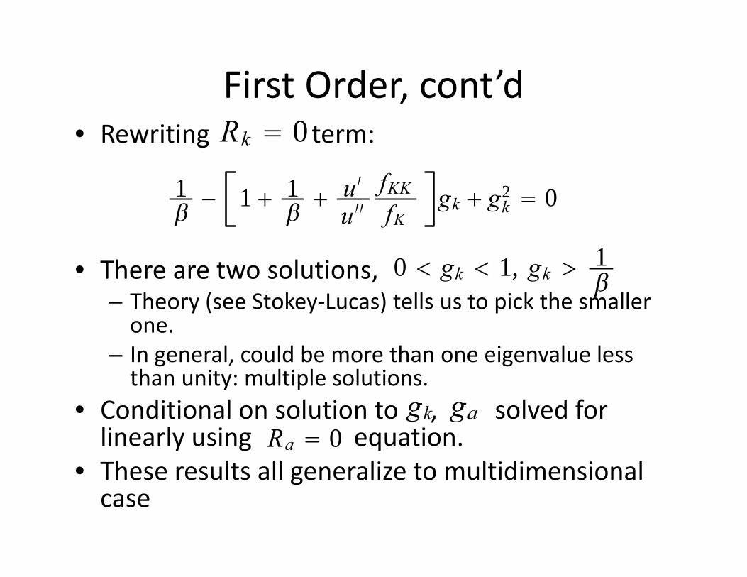
First Order, cont’d• Rewriting term:
• There are two solutions, – Theory (see Stokey‐Lucas) tells us to pick the smaller one.
– In general, could be more than one eigenvalue less than unity: multiple solutions.
• Conditional on solution to , solved for linearly using equation.
• These results all generalize to multidimensional case
Rk 0
1 − 1 1
u′u′′fKKfK
gk gk2 0
0 gk 1, gk 1
gk gaRa 0
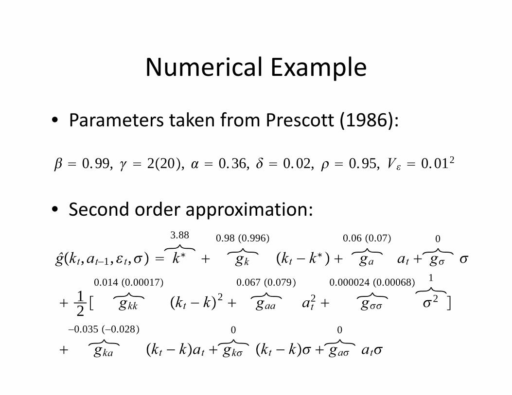
Numerical Example
• Parameters taken from Prescott (1986):
• Second order approximation:
ĝkt,at−1,t, 3.88k∗
0.98 0.996gk kt − k∗
0.06 0.07ga at
0g
12
0.014 0.00017gkk kt − k2
0.067 0.079gaa at2
0.000024 0.00068g
12
−0.035 −0.028
gka kt − kat 0
gk kt − k 0
ga at
0.99, 220, 0.36, 0.02, 0.95, V 0.012
• Following is a graph that compares the policy rules implied by the first and second order perturbation.
• The graph itself corresponds to the baseline parameterization, and results are reported in parentheses for risk aversion equal to 20.

‘If initial capital is 20 percent away from steady state, then capitalchoice differs by 0.03 (0.035) percent between the two approximations.’
‘If shock is 6 standard deviations away from its mean, then capital choice differs by 0.14 (0.18) percent between the two approximations’
Number in parentheses at top correspond to = 20.
-20 -10 0 10 200
0.005
0.01
0.015
0.02
0.025
0.03
0.035
0.04
100*( kt - k* ), percent deviation of initial capital from steady state
100*
( kt+
1 (2nd
ord
er) -
kt+1
(1st
ord
er) )
= 2 = 20
-20 -10 0 10 200
0.02
0.04
0.06
0.08
0.1
0.12
0.14
0.16
0.18
100*at, percent deviation of initial shock from steady state
100*
( kt+
1 (2nd
ord
er) -
kt+1
(1st
ord
er) )

Conclusion
• For modest US‐sized fluctuations and for aggregate quantities, it is reasonable to work with first order perturbations.
• First order perturbation: linearize (or, log‐linearize) equilibrium conditions around non‐stochastic steady state and solve the resulting system. – This approach assumes ‘certainty equivalence’. Ok, as a first order approximation.
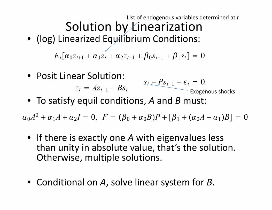
Solution by Linearization• (log) Linearized Equilibrium Conditions:
• Posit Linear Solution:
• To satisfy equil conditions, A and Bmust:
• If there is exactly one A with eigenvalues less than unity in absolute value, that’s the solution. Otherwise, multiple solutions.
• Conditional on A, solve linear system for B.
Et0zt1 1zt 2zt−1 0st1 1st 0
st − Pst−1 − t 0.zt Azt−1 Bst
0A2 1A 2I 0, F 0 0BP 1 0A 1B 0
List of endogenous variables determined at t
Exogenous shocks