Persuading the Regulator To Wait∗

Dmitry Orlov† Andrzej Skrzypacz‡ Pavel Zryumov§

First Draft: 13th February, 2016

Abstract

We study a Bayesian persuasion game in the context of real options. The Sender (firm) chooses

signals to reveal to the Receiver (regulator) each period but has no long-term commitment

power. The Receiver chooses when to exercise the option, affecting welfare of both parties.

When the Sender favors late exercise relative to the Receiver but their disagreement is small,

in the unique equilibrium information is disclosed discretely with a delay and the Receiver

sometimes ex-post regrets waiting too long. When disagreement is large, the Sender, instead

of acquiring information once and fully, pipets good information over time. These results shed

light on the post-market surveillance practices of medical drugs and instruments by the FDA,

and the role of pharmaceutical companies in keeping marginally beneficial drugs in the market.

When the Sender favors early exercise, the lack of commitment not to persuade in the future

leads to unraveling, in equilibrium all information is disclosed immediately. In sharp contrast

to static environments, the ability to persuade might hurt the Sender.

1 Introduction

Consider a pharmaceutical firm selling an FDA-regulated drug or medical device. When the drug is

first introduced, its efficacy is somewhat uncertain. As more and more patients use it, information

about its effects, the good ones and the bad ones, is gradually revealed. The regulator (FDA), monitors

this news and can recall the drug (i.e. remove it from the market) if it turns out to be unsafe. While

the firm does not want to sell a bad drug, it is natural to expect a partial misalignment between the

firm and the regulator over when to exercise the real option of recalling the drug. For example, if the

firm does not fully internalize all the costs of a bad drug, it would prefer to wait longer for stronger

∗We thank Mike Harrison, Johannes Horner, Ron Kaniel, Eric Madsen, and seminar participants at the Universityof Rochester for useful comments and suggestions.†University or Rochester, Simon School of Business. dmitry.orlov@simon.rochester.edu‡Stanford University, Graduate School of Business. andy@gsb.stanford.edu§University of Pennsylvania, Wharton School. pzryumov@wharton.upenn.edu

1

evidence of side effects than the regulator would. Similarly, if the regulator discounts future more

than the firm, it would choose to exercise the real option sooner than the firm would want it to. The

firm cannot pay the regulator to postpone a recall, but can persuade it to wait by providing additional

information/tests.1

In this paper we analyze a model of dynamic persuasion of the regulator by the firm and characterize

equilibrium dynamics of information provision. The firm and the regulator learn jointly from public

news about quality of the product produced by the firm (e.g. drug efficacy). The regulator has the

power to stop the marketing of the product at any time (i.e. he has the decision rights over the

execution of the real option) and we assume it is rational and forward-looking.

In addition to the public news, the firm can at any time run additional tests that provide a noisy signal

of product quality. The firm’s decision is what information to acquire and when. In most of the paper

we assume that the firm cannot perfectly learn the state via tests. This assumption is motivated by

the observation that short-term tests are not perfectly informative about long-term effects of a drug

and the regulator cares both about the short and long-term effects.2 The design and timing of the

tests is chosen by the firm - the regulator interprets the results of the tests, but does not have the

power to compel the firm to take them. The firm does not have private information about the quality

of the product and we assume that when it runs a test it cannot hide the results from the regulator.3

Beyond pharmaceutical firms and their regulators, our model applies to many economic situations in

which one agent has decision rights over a real option and another agent controls some information

acquisition (and there is misalignment of incentives). One example is environmental regulation: for

instance, information about price of oil or local risks of a given oil well comes gradually to the market,

and the firm can let engineers perform additional tests about the environmental impact of the well.

Another example is decision making within organizations: for instance, a product manager and a

CEO learn over time about profitability of a product and the product manager can perform market

tests. While the manager may be paid for performance, as long as the contract does not fully align

incentives, the manager will have incentives to manipulate information acquisition to influence CEO’s

1For example, see “Guidance for Industry and FDA Staff. Postmarket Surveillance Under Sec-tion 522 of the Federal Food, Drug and Cosmetic Act” issued on April 27, 2006 and availableat http://www.fda.gov/downloads/medicaldevices/deviceregulationandguidance/guidancedocuments/ucm072564.pdf.Under these FDA guidelines, the manufacturer has the opportunity to provide additional information and identifyspecific surveillance methodologies before the FDA issues postmarket surveillance. The FDA does not require con-trolled clinical trials to address its concerns, but “intend(s) that manufacturers use the most practical least burdensomeapproach to produce a scientifically sound answer.”

2Additionally, very accurate tests may be prohibitively costly, but we abstract away from any direct costs of testing.3We do not allow the firm to secretly run tests about the drug and hide unfavorable results and we assume that the

information is verifiable since it comes from scientific tests. While voluntary non-disclosure is legal in some markets,we focus on markets in which either full disclosure is mandated or the agent cannot hide having information (if theregulator knows that the firm has verifiable information then due to standard unraveling arguments the firm wouldreveal it). The analysis of fraud related to disclosure or fabrication of results is of its own interest, especially given thefamous examples of firms knowingly hiding negative effects of their products. While our paper can help understand theincentives to engage in such fraud, a proper analysis of fraud and fraud prevention is beyond the scope of this paper.

2

decision to terminate the project. Finally, the model can also apply to stakeholders’ decisions when

to sell off firm’s assets: for example, some stakeholders may have access to sources of information

while others may have the majority required to make the decision to sell assets and their preferences

need not be perfectly aligned. The key assumptions of the model are that the regulator cannot be

paid by the firm to delay a recall, the regulator cannot pay the firm to disclose information and both

parties have no commitment to future actions. For tractability, we also assume that the underlying

state and signal are binary, time is continuous and information comes to the market via a Brownian

motion with a drift that depends on the true state.

The incentives to acquire information depend on the misalignment of preferences between the firm

and the regulator. On one hand, information improves decisions so if there was no misalignment,

the firm would acquire information immediately. On the other hand, information affects when the

regulator recalls the drug - it can either speed up or delay it.4 For example, if the regulator expects

to reveal information in near future, it may find it optimal to delay the recall.

Persuasion to Wait. In the main part of the paper we assume that the firm/Sender is “more

patient” than the regulator/Receiver in the sense that absent any information from the firm, the

regulator would exercise the real option sooner than the firm would like to. So it is in the firm’s

interest to persuade the regulator to wait. In this case, we show that this game has a unique Markov-

perfect equilibrium (Markov in beliefs) in which the Sender delays information disclosure and the

Receiver sometimes ex-post regrets waiting too long. For a given prior, we show that the pattern of

information disclosure depends on the amount of disagreement between the firm and the regulator

when to recall the drug.

When the misalignment is small, then in equilibrium the firm postpones information acquisition until

its beliefs reach a point that in the event the noisy signal would deliver bad news about the drug,

the firm would want to recall the drug itself. In that case the firm acquires information once and

disclosure is fully revealing. The regulator, not wanting to take a potentially effective drug off the

market, and expecting the firm to provide comprehensive information when beliefs become sufficiently

pessimistic, waits in equilibrium for the firm to provide information. This can mean that the regulator

waits past a belief threshold at which it would stop with only public news. Finally, the timing of the

recall has a “compromise” property: in case the test results are bad, the regulator recalls the drug at

the firm’s optimal belief; when the test results are good, the regulator further delays the recall but

if he eventually does recall, it is at the regulator’s optimal threshold. This seems to correspond to

the two types of recalls in the market: in some instances the regulator suggest the firm a voluntary

4In the special case when the firm can perfectly learn the quality of the drug, as long as the misalignment ofpreferences is not so extreme that the firm would prefer to market even a bad drug, the firm would reveal thatinformation immediately. Signal imprecision creates more interesting equilibrium dynamics.

3

recall and the firm decides to follow the recommendation and in some cases the regulator recalls the

drug in opposition to the firm. This “compromise” property implies also that even if the information

about test results was not verifiable, the equilibrium would be robust - when the news is bad it is in

the firm’s self-interest to recall the drug, so seeing the firm not recalling the drug, the regulator would

rationally infer that the news is good and optimize accordingly. When the news is bad, the regulator

has ex-post regret that it waited, but since it wants to avoid a false-positive of recalling a good drug,

ex-ante it is willing to wait for the information.

When the misalignment is large, equilibrium information provision is radically different. We show that

instead of acquiring information once and fully, the firm “pipets” good information. That is, once the

regulator reaches its recall threshold, which in equilibrium is the same as if the regulator acted on

the public news only, the firm reveals just enough information to either slightly reduce the belief or

to fully reveal bad information. In the jargon of real options, the regulator’s belief threshold becomes

a reflecting boundary (and the reflection is accompanied by a jump of beliefs that the drug is bad,

so that beliefs are martingales).5 Somewhat surprisingly, while this strategy helps the firm obtain

higher payoffs than with no access to additional information, for the regulator additional information

pipetted this way has no value.

Persuasion to Act. We also discuss the case where the Sender is less patient than the Receiver, in

the sense that its threshold for exercising the real option is lower than the Receiver’s. For example, if

the real option is to invest into project that the Sender likes, or stop a project that the Sender does

not like but cannot stop on its own.6 We call this case persuasion to act.

In that case there always exists a Markov-perfect equilibrium in which the Sender immediately acquires

all information about the noisy signal. While in some cases this is beneficial for the Sender who wants

to speed-up the execution of the real option, it can be also harmful. For example, if the regulator’s

prior is above its threshold for execution based solely on the public news, and the posterior belief

after bad news lies in between the firm’s and regulator’s thresholds, the firm is hurt by equilibrium

disclosure. Unlike the case of persuasion to wait, where having access to the noisy signal is always

beneficial for the Sender, in the case of persuasion to act, this access can be detrimental for the Sender.

Moreover, we show that for some parameter values if the Sender is less patient than the Receiver, in

all Markov equilibria the Sender is worse off as a result of having access to additional information.

5If the misalignment is large enough, this is the only type of information disclosure on the equilibrium path. Whenmisalignment is intermediate, the equilibrium starts in the “pipetting” mode and if the bad news do not arrive, changesto the “waiting for full information” mode.

6In case the drug manufacturer faces triple penalties if the drug turns out to be bad, it is possible that it would liketo recall the drug even sooner than the regulator; since firms have the right to self-recall a product that situation doesnot create frictions. Therefore our analysis of persuasion to act applies more to regulator’s approval of a product or toa product manager who would like to start a new project and hopes to persuade the CEO to re-assign her.

4

On the technical side, we have decided to write the model in continuous time to use the standard

tools of real-option analysis. The drawback of this approach is that we have a game between two

strategic agents instead of a single-decision maker, and the actions are perfectly observable (unlike

in Sannikov (2007)). In general, modeling games in continuous time is notoriously difficult (see for

example, Simon and Stinchcombe (1989)). In discrete-time communications games, it is customary to

define the Sender’s strategy as a choice of message sequences from some abstract message space as a

function of the history. This can be simplified in Bayesian persuasion problems since it is without loss

of generality to describe communication by posterior beliefs induced by messages and the set of all

possible communications as the set of all distributions that satisfy the martingale property of beliefs.

Even that turns out to be technically cumbersome in continuous time. Instead, we propose to define

the Sender’s strategy to be a choice of information partition about the additional signal, and we put

constraints on the information partitions to be a well-defined filtration. Such filtrations capture a

general way the Sender can in continuous time provide information about the noisy signal in response

to the public news. While continuous time implies that for some Markov strategies of the Receiver

(mappings from beliefs about the state and noisy signal to the decision to exercise the option or not)

there does not exist a Sender’s best response (because the supremum over responses is not attainable),

the problem does not lead to non-existence of Markov equilibria.

1.1 Related Literature.

Our technology of information acquisition and disclosure is the same as in the literature on Bayesian

persuasion, as in Aumann and Maschler (1995) and Kamenica and Gentzkow (2011). That is, the agent

does not have private information, chooses how to “split” a prior belief and cannot hide results. In that

literature there are a few papers that study dynamic information disclosure, for example, Renault,

Solan, and Vieille (2014) and Ely (2015). There are many differences between these two papers and

our model. First, in their models the Sender cares only about the Receiver’s actions, while in our paper

the Sender’s preferences over actions depend on the underlying state: if the state is bad, the firm wants

to recall the drug, but if the state is good, it does not want it to do so. The second is that we have two

long-lived players and consider non-commitment equilibria rather than design of dynamic information

acquisition with dynamic commitment. Despite these important modeling differences, somewhat

surprisingly we find that in some instances the equilibrium information provision features “pipetting”

which in continuous time is equivalent to the “greedy” strategy from their results: releasing the least

information possible to prevent the recall. While pipetting is sometimes an equilibrium outcome, we

have also identified important cases when information is instead revealed only once and fully.7

7Another difference is that absent information acquisition, beliefs in those two papers drift because the underlyingstate changes, while in our model the state does not change but beliefs respond to public news. Therefore, in our paper

5

Our paper is also somewhat related to literature on voluntary dynamic information disclosure with

verifiable information, as in Acharya, DeMarzo, and Kremer (2011) or Guttman, Kremer, and Skrzy-

pacz (2014). The main difference between these models is that in our model the firm decides when

to acquire information and has to reveal all news it obtains, while in those models the firm learns

exogenously and privately: the “Receiver” in those paper is the market who does not know if the

agent obtained the news. Moreover, in those papers the agent can decide to hide bad information,

something we do not allow motivated by markets where such withholding of information would be

illegal (or where due to unraveling argument such hiding would not happen in equilibrium). We think

our model applies better to either markets with regulation compelling firms to disclose certain types

of information, or to internal-organization situations where agents may not be able to hide results of

tests from their managers.

Grenadier, Malenko, and Malenko (2015) and Guo (2014) consider two variants of dynamic models of

experts providing information to a principal with decision rights and partial misalignment of incentives.

The difference from our model is that their Senders are privately informed and provide information

via cheap talk. This leads to qualitatively different information disclosure in equilibrium. The main

similarity is that like in our paper, the dynamics of information disclosure depend on the direction

of misalignment of incentives between the Sender and Receiver. For example, in Grenadier, Malenko

and Malenko (2015) when the Sender is more patient, in equilibrium information is revealed fully but

the Receiver takes action ex-post too late; when the Receiver is more patient, information is partially

pooled in equilibrium.

The observation that in some of our equilibria the regulator waits for the additional news to arrive

is somewhat reminiscent of the results in Kremer and Skrzypacz (2007) and Daley and Green (2012)

where the expectation of news arriving to the market leads to a market breakdown due to adverse

selection.

The rest of the paper is organized as follows. In the next section we present the model. In Section 3

we provide some additional notation and preliminary results. In Section 4 we discuss persuasion to

wait. In Section 5, persuasion to act. We conclude in Section 6. The Appendix contains proofs of all

our formal results.

beliefs are martingales not only within a period but also across periods, which is not true in their papers.

6

2 Model

2.1 Basic Setup

We start with an informal description of the model. There are two long-lived players, a firm and

a regulator, who we also refer to as the Sender (she) and Receiver (he). The firm/Sender sells a

product, for example a drug or a medical device, that is either safe or unsafe, which we refer to as

the state. The players share a common prior about the state. Over (continuous) time public news

arrives about the state - information can come from payoffs or other sources, for example reports on

side effects or long-term effects of the product. We model this information as a Brownian motion

with a drift that depends on the state. Additional information can be acquired by the firm about a

noisy indicator of the state. As long as the drug is on the market, the players earn payoff flows that

on average depend on the state. Expected payoff flows are positive if the drug is safe and negative if

not (we also consider the case when they are always positive for the firm/Sender). Profits are noisy

and do not immediately reveal the state, especially that some consequences of the sales today are

delayed with long-term negative effects on the patients. The regulator has control rights over product

recall and faces a real-option problem of deciding when to recall the product from the market - his

Markov strategy is stopping time that depends on beliefs and he wants to recall unsafe drugs but

protect safe ones. We model the firm’s actions as the option to acquire information about a binary

random variable that is correlated with the state. This information is noisy because some long-term

effects of the product cannot be perfectly discovered with short-term tests or because running fully

revealing tests is prohibitively expensive. The firm’s Markov strategy is a mapping from beliefs to an

information acquisition policy that we model as a filtration. We assume that the Sender can decide

not to learn certain information, but once she obtains it, she has to disclose it. As a result, at all

times the players have the same beliefs about the state. The Receiver makes his decisions based on

the exogenous public news and the additional information chosen by the Sender; his option value of

waiting for more information depends on both the variance of the public news and the expectation

of the Sender’s future disclosures. We characterize Markov Perfect Equilibria in which the strategies

of both players depend on the current beliefs about the state of the drug and the realization of the

additional random variable the Sender can disclose.

Players and Payoffs. There are two long-lived players: a firm/Sender/she and a regulator/Receiver/he.

The firm sells a product that can be either safe θ = 0 or unsafe θ = 1.

Time is continuous and infinite. As long as the product is on the market, it generates for the firm

expected profit flow which depends on the state: Fθ ∈ F0, F1, with F0 ≥ F1 and F0 > 0. It also

generates expected welfare flow for the Regulator, Wθ ∈ W0,W1, with W0 > 0 > W1.

7

If the product is recalled from the market at time τ then the expected payoffs of the Sender and the

Receiver conditional on θ are

uS(τ, θ) =

∫ τ

0

e−rSt(F1θ + (1− θ)F0)dt uR(τ, θ) =

∫ τ

0

e−rRt(W1θ + (1− θ)W0)dt, (1)

where rS and rR are the discount rates of the two players. We allow the discount rates and payoff flows

of the two players to be different. If F1 < 0, then under complete information the two players agree on

recall policy (since their payoff flows conditional on θ have the same sign). The friction/disagreement

is caused by uncertainty about the state and hence misalignment between the Sender and the Receiver

about the option value of waiting for additional information.

Denote by Hτ the sigma-algebra reflecting all the information available to the parties at the time of

the drug recall τ , and let pτ = P(θ = 1 |Hτ ). Then the expected unconditional payoffs can be written

as

E [uS(τ, θ)] = E

[∫ τ

0

e−rSt(F1θ + (1− θ)F0)dt

]=

1

rSE[F1θ + (1− θ)F0 − e−rSτ (F1θ + (1− θ)F0)

]=

1

rSE[E[F1θ + (1− θ)F0 − e−rSτ (F1θ + (1− θ)F0)

∣∣∣hτ]]=

1

rSE[F1pτ + (1− pτ )F0 − e−rSτ (F1pτ + (1− pτ )F0)

]=

1

rSE [F1pτ + (1− pτ )F0] +

1

rSE [vS(τ, pτ )]

=1

rS

[F1p0 + (1− p0)F0

]+

1

rSE [vS(τ, pτ )] ,

where

vS(τ, p) = e−rSτ[(F0 − F1)p− F0

], (2)

Analogously for the Receiver, define vR(τ, p) as

vR(τ, p) = e−rRτ[(W0 −W1)p−W0

]. (3)

Note that expected values of vS and vR are affine transformations of the expected values of uS and

uR with a positive slope. Therefore, they define the same preferences over stopping times. For

convenience, in the rest of the paper we work with vR and vS instead of the original utility functions

given by (1).

8

Remark about Payoffs This last observation allows us to apply our model to a wider class of

real-option problems. Motivated by the drug recall application we derived preferences of the players

vS and vR from the model primitives (Fθ,Wθ). Yet, our model is applicable to any situation in which

the players’ utilities have a form of

vi(τ, p) = e−riτ[aip− bi

]ai ≥ 0, bi > 0 i ∈ R,S.

For example, parameter bi can incorporate a fixed cost incurred at the time the option is exercised, as

in models of timing of the start of a project. Similarly, in a model of a product manager and a CEO,

it can represent the foregone private benefits of the Sender from running a project when the Receiver

stops it. The real option model has been applied to a wide array of economic decisions. Our model

is relevant to any such situation if it involves a conflict of interest between an agent who has decision

rights over stopping and an agent who has access to additional information.

Information: Public News. The state of nature θ is a random variable defined on a probability

space (Ω,F ,P) with P(θ = 1) = p0 being the common prior. Neither the Sender nor the Receiver

observe at any time the realization of θ.

Over time public news about the state θ arrive via stochastic process X:

dXt = θ dt+ σ dBt

where B = (Bt)t≥0 is a Standard Brownian Motion with respect to its natural filtration FB under

measure P. The interpretation of the news process is that it can reflect sales data as well as information

from patients and medical care providers about the effects of the product. The process of learning

is gradual because it takes time to learn about all effects of a drug and we assume outcomes of any

particular patient do not change beliefs discontinuously.8

Information: Sender’s Additional Information. Sender can choose to learn about a (typically

imperfect) signal ξ independent of the Brownian Motion B. The signal ξ is binary and has conditional

distribution matrix Q0 = (qij0 ) with qij0 = P(ξ = j|θ = i). Since the columns of Q0 add up to one, the

whole matrix can be summarized by two numbers qi0 = P(ξ = 1 | θ = i) for i = 0, 1. For our purposes,

precision of signal ξ about θ is better summarized by the beliefs this signal can induce in the absence

8To be concrete, our model encompasses the following situation: the cumulative payoffs of the two players are dF (t)= Fθdt + dZFt and dW (t) = Wθdt + dZWt where ZF and ZW are standard Brownian Motions. In this case publicinformation X is a sufficient statistic for θ given public realizations of F (t) and W (t).

9

of public news. This is given by

zi0 = P(θ = 1 | ξ = i) i = 0, 1

We normalize that z00 < z10 , i.e. the signal ξ = i is more informative about the fundamental state

being θ = i. The precision of the signal ξ determines how much information in total is available to

the Sender. For example, if z00 = 0 and z10 = 1 then the Sender has a perfect information technology

and she can potentially choose information structure that reveals the state to both agents, however,

when z00 > 0 (z10 < 1) then even perfect knowledge of the signal ξ = 0 (ξ = 1) leaves both parties

uncertain about the true state θ. We describe the information acquisition technology next.

2.2 Strategies

We cast our model in continuous time to use well-established tools and intuitions for single-agent real

option problems (see for example Dixit and Pindyck (2012)). However, since our problem is a game

and not a single-decision-maker problem, continuous time requires special care in defining strategies.

While this subsection is highly technical, it is designed to capture the following idea from discrete

time: within every “period” the public news is first realized, the Sender can then provide information

about ξ by “splitting” the prior about ξ. That is, the Sender induces some posterior distribution over

ξ subject to the martingale constraint that the average posterior belief has to be equal to the prior.

The Sender can commit within a period to an arbitrary distribution, but she cannot commit to future

actions. After that, the Receiver makes the decision to either stop or continue the project (that is, to

either recall or not the product) and he also cannot commit to future actions. The Sender’s strategy

is a function of past history of public news and information revealed about ξ up to time t. The

Receiver’s strategy is additionally a function of the information disclosed about ξ at time t. Markov

strategies depend on the history only insofar that they affect joint beliefs about θ and ξ.

Sender’s Strategy. Information available to the Sender can be organized in three groups:

1. Public Information: FX = (FXt )t≥0 with FXt = σ(Xs, s ≤ t)

2. Private Signal : Fξ = σ(ξ)

3. Randomization Device: A sufficiently rich9 filtration FR = (FRt )t≥0 such that FR∞ =∨∞t=0 FRt ,

FB∞ =∨∞t=0 FBt , and Fθ = σ(θ) are mutually independent sigma algebras10.

9For our purposes it will be sufficient to require that this filtration contains sigma-algebras generated by a countableand independent uniform random variables and Poisson processes. In the construction of equilibria, we first assumethat this filtration is sufficiently rich and then show by construction what is sufficient.

10We also require the original probability space to be rich enough to accommodate Brownian news and independentrandomization, i.e. FR∞ ⊂ F and FB∞ ⊂ F .

10

For technical reasons we require filtrations FX and FR to satisfy standard conditions, i.e., to contain

all P-null sets and to be right-continuous.

Definition. A feasible action profile of the Sender is a filtration H = (Ht)t≥0 satisfying standard

conditions such that

∀ t FXt ⊆ Ht ⊆ σ(FXt ,Fξ,FRt ). (4)

Let H denote the set of all feasible action profiles.

Such definition of action profiles allows the Sender to generate informative messages at every time

t whose distribution can be contingent on the path of X, realization of ξ, and realization of past

messages. Standard restrictions on the filtration H guarantee that all martingales with respect to

this filtration have cadlag versions and first hitting times of such martingales are stopping times with

respect to H.11 That assures that expected payoffs from our strategies are well-defined. The set of all

action profiles corresponds to the set of all possible histories of the game in case the Receiver never

stopped.12.

Note that according to this definition an action profile specifies not just current information disclosure

but a whole plan of contingent dynamic information disclosures starting at time 0. Intuitively, we are

capturing an action in a normal form of the dynamic game. To introduce a notion of perfection, we

next define histories and strategies.

Define the history generated by a feasible action profile H up to time t to be

Ht = Hs, s < t.

Notice that such definition of history in a way encompasses all paths that could happen up to time t

under the action profile H. Thus, any decisions made conditional on history up to time t would have

to specify the plan of action for every possible realization of stochastic uncertainty.

Denote by H (Ht) the set of all feasible action profiles that agree with H up to time t, i.e.

H (Ht) =H ∈H : Hs = Hs ∀ s < t

. (5)

Definition. A strategy of the Sender, S, is a mapping from any possible history Ht into the set of

all feasible action profiles H (Ht) that agree with Ht up to time t, i.e.

S(Ht) ∈H (Ht). (6)11For further details see Pollard (2002).12We chose H to denote the set of all action profiles motivated by Mailath and Samuelson (2006) who use that

symbol to denote the set of all histories of a repeated game

11

At any time and after any history of the game, the Sender’s strategy S is a choice of an action profile,

i.e. it specifies the whole structure of past and future information sharing, S(Ht). Since the history

states what already happened and an action profile specifies information sharing starting at time 0,

the strategy at time t can only choose actions that are consistent with the realized history.

Note that in discrete-time games it is more common to define a strategy as a mapping from all possible

histories to current period information disclosure. Iteratively one can then recover the whole sequence

of actions in the future periods and specify the information filtration chosen by the Sender. We

define the strategy to be the whole contingent plan of disclosures in current and future periods. Such

definition allows us to avoid some technical issues related to continuous time modeling.

A strategy of the seller is time consistent if

S(Ht) = S(S(Ht)t

′)∀ t′ > t ≥ 0 and ∀H ∈H .

In words, if the Sender decides on the whole structure of information sharing at time t after arbitrary

history Ht and follows it up to some future time t′, then at t′ (for a strategy to be time consistent)

she should not change her mind given the history S(Ht)t′ = Ss(Ht), s < t′. We will not restrict the

Sender to time consistent strategies, allowing her to deviate to non-time consistent strategy after any

time (yet, time consistency will be a feature of the equilibrium due to sequential rationality).

Remark. Our model can be described as a dynamic Bayesian persuasion model without commit-

ment. In Bayesian persuasion models, Sender’s strategy is typically defined either as a choice of

messages, or, more commonly, as a choice of posterior distribution of beliefs subject to a martingale

constraint. In our definition, instead of choosing posteriors, the Sender chooses filtration/sigma-

algebras of the set Ω and they induce posterior beliefs, so that in discrete time the definitions are

equivalent. While it may be possible to define a strategy in continuous time using posterior beliefs,

we find it more convenient to define actions in terms of the filtrations as they are a more fundamental

object. Also recall that we assume that the filtration chosen by the Sender up to time t is public,

so that at any time the Sender and Receiver’s beliefs coincide. This captures our assumption that

the firm can decide not to learn about some aspects of its drug, but if it learns something, it has to

disclose it to the regulator.

We define a (Markov) state of the game, π, to be the joint distribution of a pair (θ, ξ). That is, π

contains information about the posterior belief about the pay-off relevant state θ, about the realization

of the Receiver’s signal ξ, and about the correlation between the two. Denote by Π the set of all possible

joint distributions of the pair (θ, ξ).

12

For any feasible action profile of the Sender H = (Hs)s≥0 ∈ H and arbitrary time t define the

posterior belief about the state π to be:

πt− = Law(θ, ξ |Ht−).

Definition (Markov Strategy of the Sender). A strategy of the Sender, S, is Markov in state π

if for any feasible action profile H ∈H and any time t ≥ 0 the induced belief process (πt+s)s≥0 with

πt+s = Law(θ, ξ |St+s(Ht))

is a Markov process.

Verbally, we define the strategy to be Markov, if the future evolution of posterior beliefs about (θ, ξ),

that are induced jointly by public news and the Sender’s information disclosure, depend only on

current beliefs. Also note that since in our game the Sender never has private information, posterior

beliefs are uniquely pinned down for any history Ht, both on and off the equilibrium path.

Receiver’s Strategy. We now turn to the Receiver’s strategy.

Definition. A strategy of the Receiver, T , is a collection of stopping times. For any action profile

of the Sender H and any time t ≥ 0, T (H, t) is a stopping time with respect to H that takes values in

[t,+∞).

Intuitively, T (H, t) is the Receiver’s optimal time of exercising the option calculated from the time

t stand point given the history Ht up time t, the latest information Ht available at time t, and

expectations about future information sharing given by H.

Similarly to the Sender’s strategy, we now define the strategy of the Receiver which is Markov in the

state π.

Definition (Markov Strategy of the Receiver). A strategy of the Receiver T is Markov in state

π if there exists a set T ⊆ Π such that

∀H ∈H , t ≥ 0 T (H, t) = infs ≥ t : πs ∈ T, (7)

where πs = Law(θ, ξ |Hs)

In words, the Receiver’s strategy is Markov if the decision to stop depends only on the beliefs induced

by Ht and nothing else. In particular, if the Sender deviates from the equilibrium path but later

13

follows disclosure that would bring beliefs back to the equilibrium path, the Receiver cannot punish

such behavior and has to behave the same way as if that belief was reached on-path.

Heuristically, the sequence of actions in a short period of time dt is shown in Figure 1 and can

be described as follows: for a given ω ∈ Ω (i) first, the public news Xt(w) is realized, (ii) second,

additional information from St(Ht) is announced (iii) finally, the Receiver upon observing everything

prior decides whether to exercise the option or not.

dt

Public NewsXt Arrive

Additional InformationFrom St(Ht) is announced

ReceiverActs/Waits

Figure 1: Timing of Events in a Short Interval of Time

2.3 Equilibrium.

Now, we define equilibrium that is Markov in posterior beliefs, π.

Definition. A Markov Perfect Equilibrium in posterior beliefs, π, is a collection of Markov strategies

of the Sender and Receiver (S∗, T ∗) such that

1. The Receiver’s Strategy T ∗ is optimal given the anticipated flow of information S∗, i.e.

∀H ∈H ,∀ t ≥ 0 T ∗(H, t) ∈ arg maxτ∈M(S∗(Ht)),τ≥t

E[vR(τ, pτ )

](8)

where ps = P(θ = 1 |S∗s (Ht)) and the maximum is taken over the set of all stopping times

M(S∗(Ht)) with respect to filtration S∗(Ht).

2. The Sender’s strategy S∗ is optimal given the anticipated stopping rule of the Receiver T ∗, i.e.

∀H ∈H ,∀ t ≥ 0 S∗(Ht) ∈ arg maxH∈H (Ht)

E[vS

(T ∗(H, t), pT ∗(H,t)

) ](9)

Notice that in the spirit of subgame perfection, we require both the strategy of the Sender S∗ and

the strategy of the Receiver T ∗ to be optimal after arbitrary histories of the game, even those that

do not occur along the equilibrium path.

14

3 General Analysis

In this section we provide some preliminary analysis that facilitates delivery of our main results in

the next two sections.

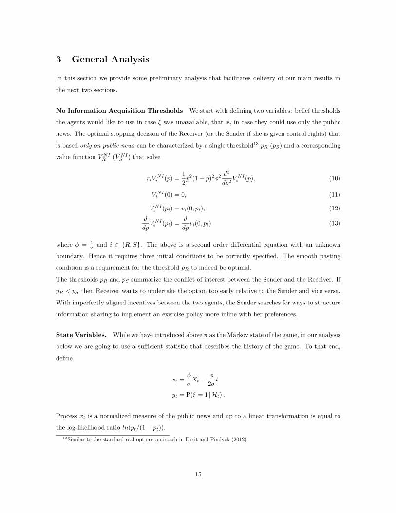
No Information Acquisition Thresholds We start with defining two variables: belief thresholds

the agents would like to use in case ξ was unavailable, that is, in case they could use only the public

news. The optimal stopping decision of the Receiver (or the Sender if she is given control rights) that

is based only on public news can be characterized by a single threshold13 pR (pS) and a corresponding

value function V NIR (V NIS ) that solve

riVNIi (p) =

1

2p2(1− p)2φ2 d

2

dp2V NIi (p), (10)

V NIi (0) = 0, (11)

V NIi (pi) = vi(0, pi), (12)

d

dpV NIi (pi) =

d

dpvi(0, pi) (13)

where φ = 1σ and i ∈ R,S. The above is a second order differential equation with an unknown

boundary. Hence it requires three initial conditions to be correctly specified. The smooth pasting

condition is a requirement for the threshold pR to indeed be optimal.

The thresholds pR and pS summarize the conflict of interest between the Sender and the Receiver. If

pR < pS then Receiver wants to undertake the option too early relative to the Sender and vice versa.

With imperfectly aligned incentives between the two agents, the Sender searches for ways to structure

information sharing to implement an exercise policy more inline with her preferences.

State Variables. While we have introduced above π as the Markov state of the game, in our analysis

below we are going to use a sufficient statistic that describes the history of the game. To that end,

define

xt =φ

σXt −

φ

2σt

yt = P(ξ = 1 |Ht) .

Process xt is a normalized measure of the public news and up to a linear transformation is equal to

the log-likelihood ratio ln(pt/(1− pt)).13Similar to the standard real options approach in Dixit and Pindyck (2012)

15

Next, define the most extreme posteriors about θ that the Sender can induce at any time t as

z1t = P(θ = 1 |ξ = 1,Ht) , z0t = P(θ = 1 |ξ = 0,Ht) .

Lemma 1. Given prior (p0, z00 , z

10), pair (xt, yt) is a sufficient statistic for posterior beliefs (pt, z

0t , z

1t ).

Proofs of all formal results are in the Appendix. For intuition, notice that z1t and z0t evolve based only

on the new information revealed by the public news. Thus, we can write z1t = z1(xt) and z0t = z0(xt).

The remaining parameter yt allows to recover belief about θ as pt = ytz1(xt) + (1− yt)z0(xt). Thus,

the state (pt, z0t , z

1t ) (or, equivalently, state (pt, q

0t , q

1t )) maps naturally into (z0(xt), z

1(xt), yt) and we

can treat the pair (xt, yt) as the new state variable, which we do in the rest of the paper.

The benefit of using (x, y) instead of (pt, q0t , q

1t ) is that when the Sender discloses information about

ξ, it changes both the beliefs about θ and ξ, while in the (x, y) space, only y changes. That facilitates

characterization of the Sender’s value function. Revelation of public new over time, on the other

hand, affects both xt and yt. Define yt to be the non-strategic component of yt, i.e. the belief about

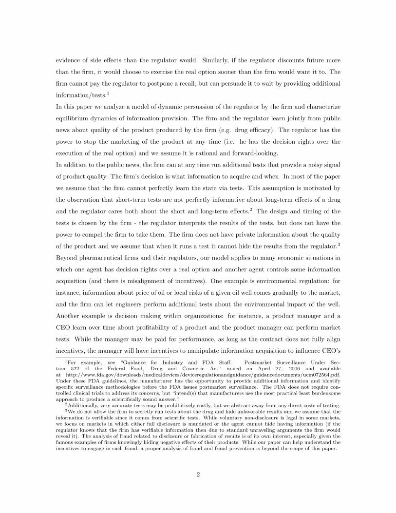
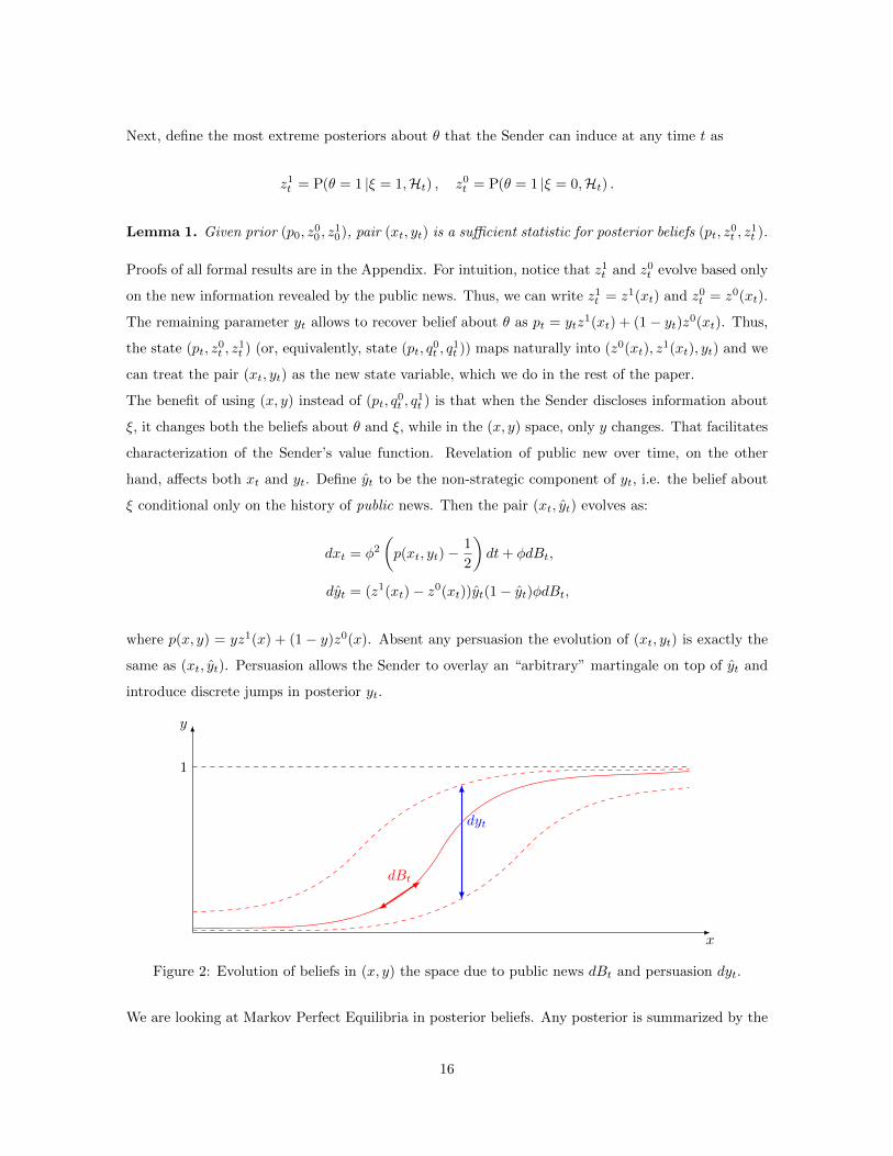
ξ conditional only on the history of public news. Then the pair (xt, yt) evolves as:

dxt = φ2(p(xt, yt)−

1

2

)dt+ φdBt,

dyt = (z1(xt)− z0(xt))yt(1− yt)φdBt,

where p(x, y) = yz1(x) + (1 − y)z0(x). Absent any persuasion the evolution of (xt, yt) is exactly the

same as (xt, yt). Persuasion allows the Sender to overlay an “arbitrary” martingale on top of yt and

introduce discrete jumps in posterior yt.

x

y

1

dBt

dyt

Figure 2: Evolution of beliefs in (x, y) the space due to public news dBt and persuasion dyt.

We are looking at Markov Perfect Equilibria in posterior beliefs. Any posterior is summarized by the

16

pair (xt, yt). In a given MPE denote the value function of the Receiver and Sender by VR(x, y) and

VS(x, y) respectively. We now provide characterization of these value functions for given strategies of

the opponent.

Sender’s Best Response. We start with the Sender’s value function and show that it solves an

HJB equation and a fixed point of a concavification operator (familiar from Bayesian persuasion

literature). Which of the two applies depends on whether beliefs (x, y) are the extreme point of a

lower contour set of VS(x, y). Then, given a value function, we construct a strategy that achieves

it. It has the property that in those points where HJB is satisfied the Sender keeps quiet and in

points where the concavification applies, there is randomization between two posterior beliefs about

y. VS(x, y) is weakly concave in y since the Sender can always induce any posterior distribution over

y subject to the martingale constraint. At points where VS(x, y) is strictly concave in y it has to be

optimal to not reveal any information.

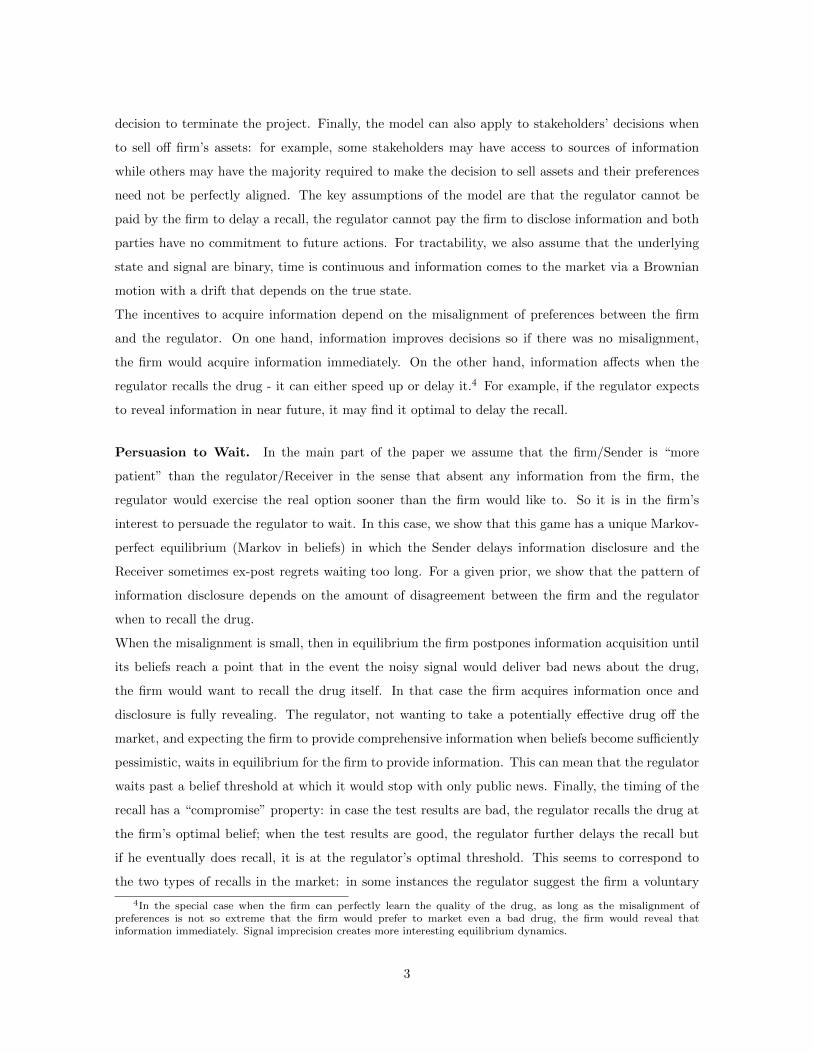
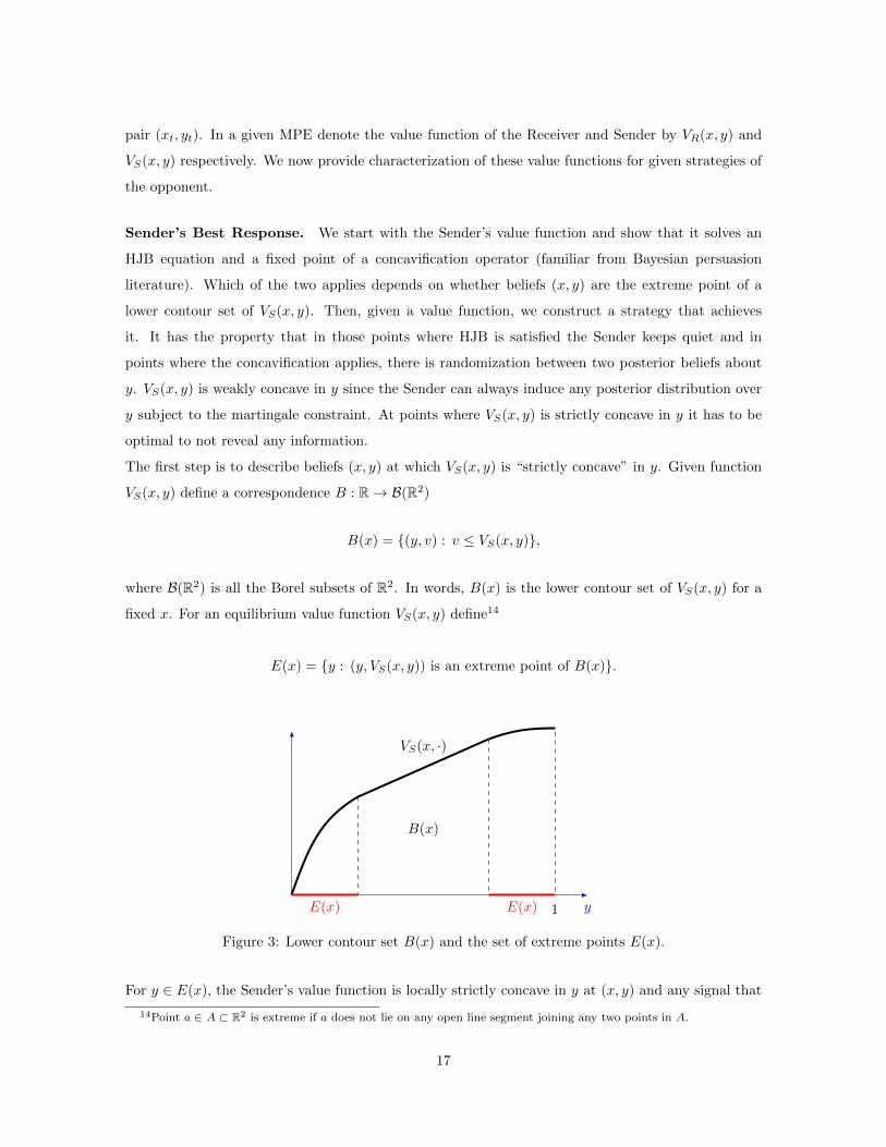
The first step is to describe beliefs (x, y) at which VS(x, y) is “strictly concave” in y. Given function

VS(x, y) define a correspondence B : R→ B(R2)

B(x) = (y, v) : v ≤ VS(x, y),

where B(R2) is all the Borel subsets of R2. In words, B(x) is the lower contour set of VS(x, y) for a

fixed x. For an equilibrium value function VS(x, y) define14

E(x) = y : (y, VS(x, y)) is an extreme point of B(x).

y

VS(x, ·)

1E(x) E(x)

B(x)

Figure 3: Lower contour set B(x) and the set of extreme points E(x).

For y ∈ E(x), the Sender’s value function is locally strictly concave in y at (x, y) and any signal that

14Point a ∈ A ⊂ R2 is extreme if a does not lie on any open line segment joining any two points in A.

17

she would generate about ξ would decrease her total payoff. Thus for y ∈ E(x) the Sender must prefer

waiting and not obtaining any additional information. For y /∈ E(x), the Sender’s value function is

locally linear in y. Hence she can send the Receiver a signal about ξ and her value function remains

unchanged.

Definition. For a function f : R → R define cav [f ] to be the smallest concave function that weakly

majorizes f .

We show that the if y ∈ E(x) then Sender’s value function satisfies a “waiting” Hamilton-Jacobi-

Bellman equation in (x, y).15 When y /∈ E(x) then Sender’s value function is a convex combination

between her value function when she waits, and her value function when she induces the Receiver to

exercise the option:

Lemma 2 (Dynamic Concavification). In any MPE Sender’s value function VS(x, y) is concave in y

and continuous in x. For every y ∈ E(x) and (x, y) /∈ T∗ function VS(x, y) satisfies

rSVS(x, y) =∂VS∂x· φ2

(p(x, y)− 1

2

)+

1

2

∂2VS∂2x

φ2 +1

2

∂2VS(x, y)

∂2y· (z1(x)− z0(x))2y2(1− y)2φ2

+∂2VS(x, y)

∂x∂y· (z1(x)− z0(x))y(1− y)φ2

(14)

Otherwise it satisfies

VS(x, y) = cavµ

[VS(x, µ) · 1 (x, µ) /∈ T∗+ vS(0, z1(x)µ+ z0(x)(1− µ)) · 1 (x, µ) ∈ T∗

](y). (15)

Notice that equation (15) is not tautological since for in the region (x, y) ∈ T∗ it might be possible for

the Sender to split the belief y into y, y and obtain a pay-off VS(x, y) > vS(0, z1(x)y+z0(x)(1−y)).

Sender Strategy Implementation. Given a function VS(x, y) that satisfies the conditions outlined

in Lemma 2 the Sender has a well-defined strategy attaining this payoff. If yt ∈ E(xt), then the Sender

does not disclose information. If yt /∈ E(xt) define

y(xt, yt) = sup y : y < yt and y ∈ E(xt)

y(xt, yt) = inf y : y > yt and y ∈ E(xt)

The Sender uses a public lottery between beliefs yt

and yt with probabilities that satisfy that beliefs

about y are a martingale.

15In fact, it is an ODE w.r.t. public belief about the fundamental p.

18

Receiver’s Best Response. We now turn to characterizing the Receiver’s equilibrium value func-

tion and strategy. We show that any MPE is outcome-equivalent to a MPE in which the Receiver

follows a threshold strategy for every x: if beliefs about ξ are below the threshold he waits and if they

are above the threshold, he stops:

Lemma 3 (Threshold Strategy). In any MPE, Receiver’s value function VR(x, y) is convex in y. For

any x the set where Receiver strictly prefers to wait is

W(x) = y : VR(x, y) > vR(0, z1(x)y + z0(x)(1− y))

is an interval [0, l(x)). Moreover, in any MPE the Receiver without loss of generality follows a threshold

strategy: wait when y < l(x), and act when y > l(x).

While the convexity of VR(x, y) in y is non-trivial, the characterization of the set W(x) follows imme-

diately from linearity of vR(0, z1(x)y+z0(x)(1−y)) in y. The second part of the Lemma 3 shows that

regardless of the Receiver’s action in the region (x, y) : y > l(x) the beliefs spend no time there,

thus, one can without loss resolve the Receiver’s indifference and focus only on threshold strategies.

Recommendation Principle. The last step in this section is to simplify the relevant set of equi-

libria further by noticing that without loss of generality we can consider equilibria in which the Sender

discloses information about ξ only to affect Receiver’s immediate action.

Definition. An MPE (T ∗,H∗) is a Recommendation Equilibrium if there exists a message process

m = (mt)t≥0 with values in 0, 1 such that

1. S∗s (Ht) = σ(Ht−, Xs,ms; s ≥ t) for all s ≥ t, t ≥ 0,H ∈H ,

2. T ∗(H, t) = infs ≥ t : ms = 1 for all t ≥ 0, H ∈H .

That is, in a Recommendation Equilibrium one can think of messages mt as recommended actions

to Receiver with mt = 0 being the recommendation to wait and mt = 1 being the recommendation

to exercise the option. Whether such class of equilibria is a restrictive may be a priori unclear. The

subtlety arises because a richer sigma algebraHt might not necessarily change the instantaneous action

of the Receiver but induce a variety of posterior beliefs affecting the continuation game. Nevertheless,

we show that it is in Sender’s best interest to simply recommend the action to the Receiver and not

reveal any additional information. The intuition behind this result it twofold: on one hand, similar

to Myerson (1986), making information set of the Receiver coarser relaxes incentive constraints. On

the other hand, coarser history up to time t expands the set of feasible actions of the Sender allowing

to secure a higher pay-off.

19

Lemma 4 (Markov Recommendation Principle). For any MPE (T ∗,H∗) there exists a Recommen-

dation Equilibrium (T , H) such that T = T ∗.

4 Impatient Receiver pS > pR

In this section we analyze the game in case pS > pR, that is, the conflict of interest is such that with

only public information, the threshold belief at which the Receiver would choose to stop is lower than

the optimal stopping point for the Sender. This case is motivated by our leading example of a drug

or a medical device and the assumption that the firm would like to further delay the decision to recall

the product at the time the regulator is just indifferent.

For any level of public news xt the posterior belief pt about θ is always between

z0(xt) ≤ pt = ytz1(xt) + (1− yt)z0(xt) ≤ z1(xt).

By revealing ξ, the Sender could “speed up” or “delay” exercise of the real option depending on the

realization of ξ, since it would move the belief closer to z1(xt) or z0(xt). Consider the incentives of the

Sender state by state: if ξ = 0 then she would prefer this information to become public as it lowers

public beliefs and delays option exercise. If ξ = 1, then the Sender wishes to exercise the option when

z1(x) ≥ pS > pR. This suggests that when z1(xt) ≥ pS , the Sender should prefer to reveal ξ because

in this case if it turns out that ξ = 1 then the Receiver would stop which is in the Sender’s best

interest, and if ξ = 0 the Receiver will delay as much as it is possible. In other words, two rounds

of eliminating dominated strategies imply that it is optimal for the Sender to reveal ξ when z1(x)

reaches pS . The following lemma established this result formally.

Lemma 5. In any MPE, if after some history the posterior z1(xt) ≥ pS, then the Sender immediately

fully reveals ξ.

If z10 = 1, then Lemma 5 fully characterizes equilibrium outcome: immediate disclosure of ξ at

t = 0 followed by option exercise as soon as pt ≥ pR. Otherwise, define x1S to be the level16 of the

(normalized) public signal at which, conditional on ξ = 1, beliefs are pS :

z1(x1S) = pS .

Lemma 5 implies as soon as the (normalized) public signal x reaches in equilibrium level xt = x1S then

the Sender immediately reveals ξ and the resulting exercise of the real option has the “compromise”

16Equation z1(x1S) = pS has a unique solution since when z10 < 1, then z1(·) is a strictly increasing function with 0and 1 being the limits at −∞ and +∞ respectively.

20

property that we described in the Introduction: Conditional on ξ = 1, the option is exercised at the

Sender’s first-best threshold, pS ; conditional ξ = 0, the option is exercised at the Receiver’s first-best

threshold, pR.

Our next step is to construct an equilibrium and discuss under what conditions x1S is reached. We

then prove that the Markov Perfect Equilibrium is essentially unique.

Receiver’s Equilibrium Strategy. When deciding whether to exercise the real option the Receiver

weights the benefits of obtaining more precise information in the future against the costs of waiting.

There are two sources of information for the Receiver: (i) public news and (ii) Sender’s persuasion.

While the amount of information the Sender shares is an equilibrium object, Lemma 5 states that

there is always full information revelation by the Sender when beliefs (x, y) are such that x ≥ x1S .

For now, assume that public information and discrete revelation when x1S are the only two sources of

valuable information for the Receiver.17

The value of learning from public news alone is given by18 V NIR (x, y) which has been defined in Section

3. If the Receiver additionally learns ξ when public news reach x1S , we denote the corresponding value

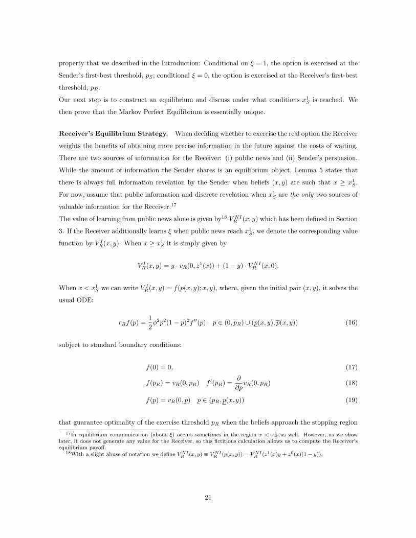
function by V IR(x, y). When x ≥ x1S it is simply given by

V IR(x, y) = y · vR(0, z1(x)) + (1− y) · V NIR (x, 0).

When x < x1S we can write V IR(x, y) = f(p(x, y);x, y), where, given the initial pair (x, y), it solves the

usual ODE:

rRf(p) =1

2φ2p2(1− p)2f ′′(p) p ∈ (0, pR) ∪ (p(x, y), p(x, y)) (16)

subject to standard boundary conditions:

f(0) = 0, (17)

f(pR) = vR(0, pR) f ′(pR) =∂

∂pvR(0, pR) (18)

f(p) = vR(0, p) p ∈ (pR, p(x, y)) (19)

that guarantee optimality of the exercise threshold pR when the beliefs approach the stopping region

17In equilibrium communication (about ξ) occurs sometimes in the region x < x1S as well. However, as we showlater, it does not generate any value for the Receiver, so this fictitious calculation allows us to compute the Receiver’sequilibrium payoff.

18With a slight abuse of notation we define V NIR (x, y) ≡ V NIR (p(x, y)) = V NIR (z1(x)y + z0(x)(1− y)).

21

(pR, p(x, y)) from below, and

f(p(x, y)) = vR(0, p(x, y)) f ′(p(x, y)) =∂

∂pvR(0, p(x, y)) (20)

(21)

that guarantee optimality of the exercise threshold p(x, y) when the beliefs approach the stopping

region (pR, p(x, y)) from above. The last boundary condition

f(p(x, y)) = y · vR(0, pS) + (1− y) · V NIR (x1S , 0). (22)

pins down from the value that Receiver derives from full disclosure of ξ: if ξ = 1 beliefs increase to pS

which leads to immediate exercise, if ξ = 0, beliefs decrease to z0(x1S) and the Receiver subsequently

exercises the real option when his beliefs reach pR. The threshold p(x, y) is an implied belief about θ

when xt = x1S , formally it is defied by

p(x, y) =pS · q0(x, y)

q1(x, y)(1− pS) + q0(x, y)pS,

q0(x, y) = (1− z1(x)) · y

1− yz1(x)− (1− y)z0(x),

q1(x, y) = z1(x) · y

yz1(x) + (1− y)z0(x).

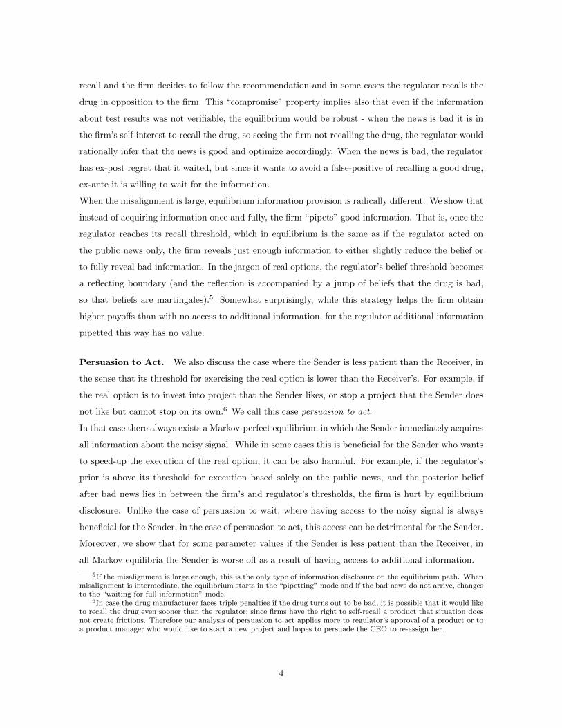
A solution to this system is illustrated in Figure 4. There are three regions of beliefs: between (0, pR)

the Receiver waits optimally because of his option to wait for public news. In (pR, p(x, y)) the Receiver

stops immediately. Finally, in (p(x, y), p(x, y)) the Receiver waits because of the option value that ξ

will be discretely revealed.

p

f(p)

Receiver’

s Value if ξis

revea

ledat x

1S

z0(x1S) pSpR p(x, y) p(x, y)

Figure 4: Receiver’s expected value f(p) from acting only on public news and the discrete messagefrom the Sender at x1S .

22

When the signal ξ is very informative, or when disagreement between Sender and Receiver is small,

then pR ≥ p(x, y), so instead of two waiting regions as in Figure 4, there is only one. In that case

the Receiver prefers to wait everywhere between p = 0 and p(x, y) until the Sender reveals ξ. In this

case f is given as a solution of the ODE (16) subject to boundary conditions (17) and (22) only. The

equilibrium is quite simple – once belief p(x, y) is reached, the Sender reveals ξ and Receiver acts

accordingly.

When ξ is not that informative or the disagreement is large, so that pR < p, the equilibrium is more

complicated. In that case, for beliefs in (pR, p), the Receiver would prefer to exercise the option,

rather than wait for the x1S threshold. For x ≤ x1S define l(x) as the minimal solution to the equation

l(x) = infy ∈ [0, 1] : vR(0, z1(x)y + z0(x)(1− y)) = V IR(x, y)

.19,20

Define a candidate Markov strategy of the Receiver, T ∗, via the following stopping set T∗:

T∗ =(x, y) : pR ≤ z1(x) ≤ pS , y > l(x)∪

(x, y) : z1(x) > pS , z0(x) ≤ pR, y = 1∪ (23)

(x, y) : z0(x) > pR

Intuitively, according to (23) the Receiver waits if the value of waiting VR(x, y) is strictly above the

value of exercising the option vR(0, p(x, y)). This happens when z1(x) < pR or when pR ≤ z1(x) ≤ pSand y < l(x). Additionally, when z1(x) > pS but z0(x) ≤ pR the Receiver anticipates immediate

revelation of ξ, thus, waiting everywhere but y = 1 is optimal. Finally, when z0(x) > pR the Receiver

exercises the option regardless of the realization of ξ. The distinction from a standard real option is

that the Receiver now has an endogenous option of waiting for the Sender to reveal ξ.21 This strategy

is depicted in Figure 5.

Sender’s Equilibrium Strategy. For x < x1S even if the signal is ξ = 1 the Sender would prefer to

wait longer to observe public news. This means that, intuitively, the Sender should try to minimize the

probability of option exercise as much as possible when x < x1S . We heuristically define the strategy

of the Sender via the messages communicated to the Receiver:

- z1(x) ≥ pS . Sender reveals ξ immediately. As we saw before, Sender obtains her highest possible

equilibrium payoff this way (she gets her most-preferred stopping when ξ = 1 and she delays

19We interpret inf∅ ≡ +∞.20Notice that p(x, l(x)) is either pR or p(x, l(x))21Additionally the Receiver waits in a measure zero subset of all states in which VR(x, y) = vR(0, p(x, y)) to make

sure that the best response of the Sender is well-defined.

23

x

y

z1(x) = pR z1(x) = pS z0(x) = pR

y=l(x)

p(x, y) = p(x, y)p(x, y) = pR

y = l(x)

R: waitS: wait

R: act

S: reflect

R: actR: wait

R: wait

S: reveal

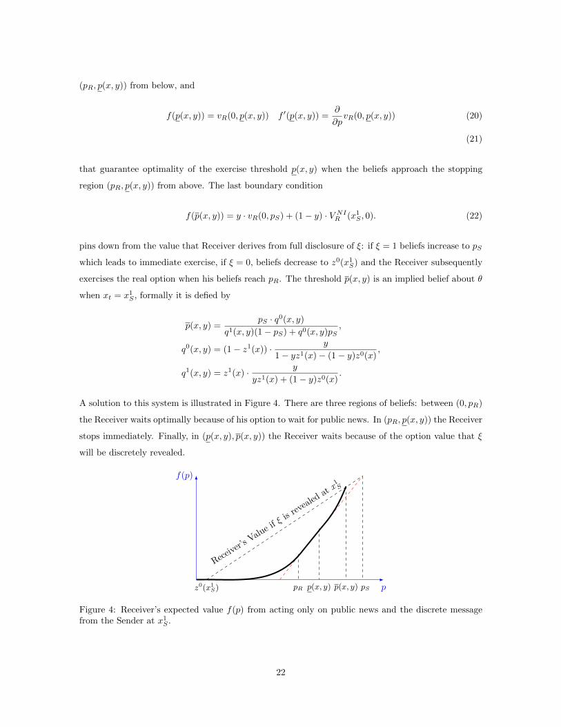
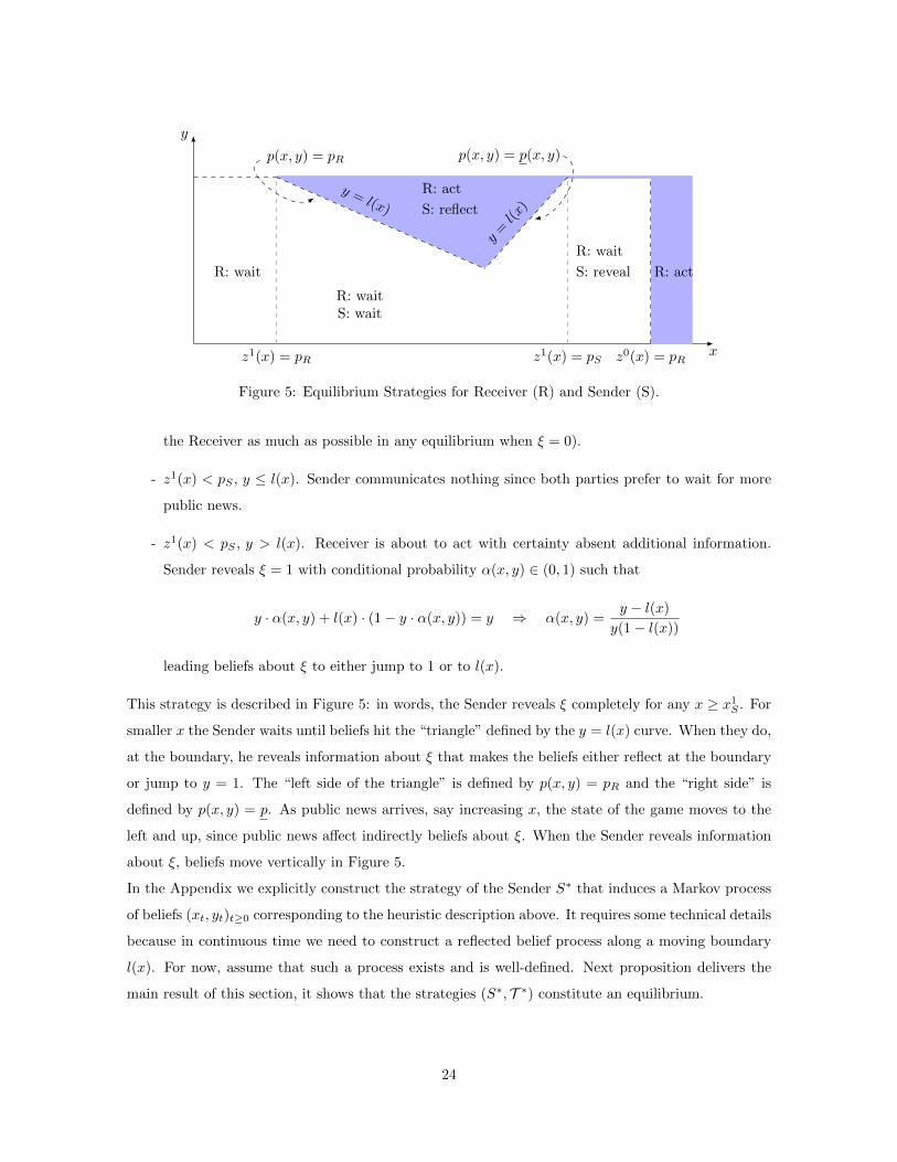
Figure 5: Equilibrium Strategies for Receiver (R) and Sender (S).

the Receiver as much as possible in any equilibrium when ξ = 0).

- z1(x) < pS , y ≤ l(x). Sender communicates nothing since both parties prefer to wait for more

public news.

- z1(x) < pS , y > l(x). Receiver is about to act with certainty absent additional information.

Sender reveals ξ = 1 with conditional probability α(x, y) ∈ (0, 1) such that

y · α(x, y) + l(x) · (1− y · α(x, y)) = y ⇒ α(x, y) =y − l(x)

y(1− l(x))

leading beliefs about ξ to either jump to 1 or to l(x).

This strategy is described in Figure 5: in words, the Sender reveals ξ completely for any x ≥ x1S . For

smaller x the Sender waits until beliefs hit the “triangle” defined by the y = l(x) curve. When they do,

at the boundary, he reveals information about ξ that makes the beliefs either reflect at the boundary

or jump to y = 1. The “left side of the triangle” is defined by p(x, y) = pR and the “right side” is

defined by p(x, y) = p. As public news arrives, say increasing x, the state of the game moves to the

left and up, since public news affect indirectly beliefs about ξ. When the Sender reveals information

about ξ, beliefs move vertically in Figure 5.

In the Appendix we explicitly construct the strategy of the Sender S∗ that induces a Markov process

of beliefs (xt, yt)t≥0 corresponding to the heuristic description above. It requires some technical details

because in continuous time we need to construct a reflected belief process along a moving boundary

l(x). For now, assume that such a process exists and is well-defined. Next proposition delivers the

main result of this section, it shows that the strategies (S∗, T ∗) constitute an equilibrium.

24

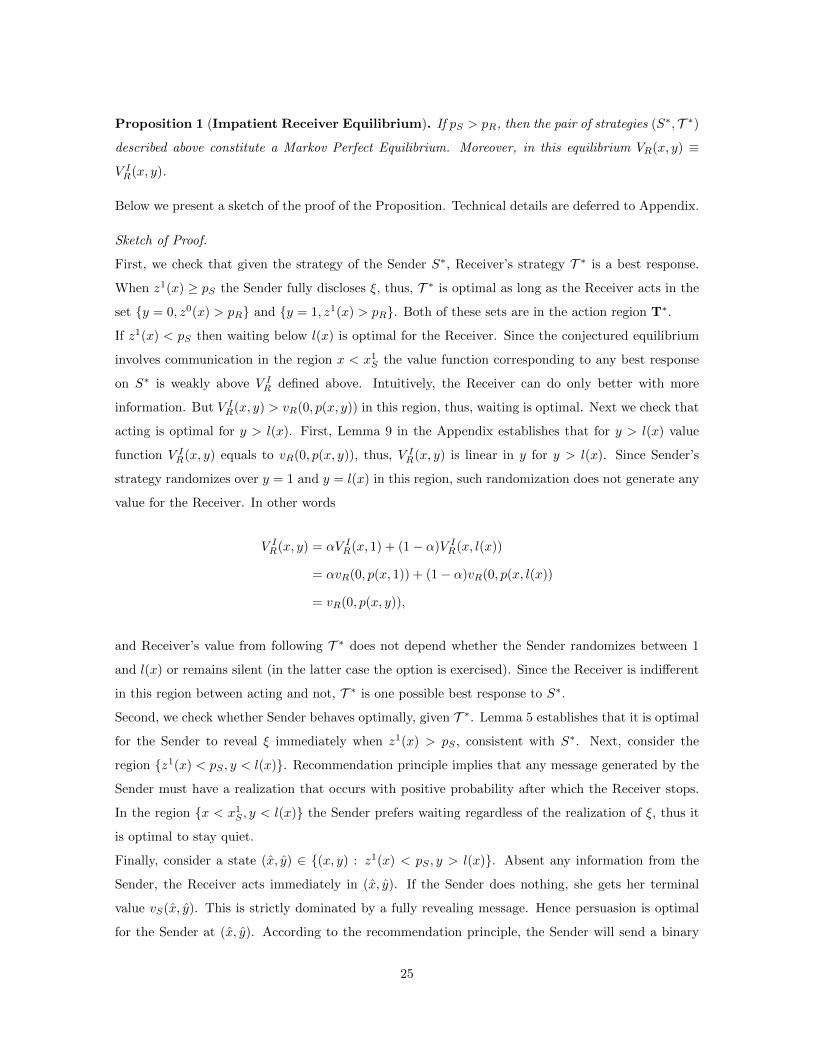
Proposition 1 (Impatient Receiver Equilibrium). If pS > pR, then the pair of strategies (S∗, T ∗)

described above constitute a Markov Perfect Equilibrium. Moreover, in this equilibrium VR(x, y) ≡

V IR(x, y).

Below we present a sketch of the proof of the Proposition. Technical details are deferred to Appendix.

Sketch of Proof.

First, we check that given the strategy of the Sender S∗, Receiver’s strategy T ∗ is a best response.

When z1(x) ≥ pS the Sender fully discloses ξ, thus, T ∗ is optimal as long as the Receiver acts in the

set y = 0, z0(x) > pR and y = 1, z1(x) > pR. Both of these sets are in the action region T∗.

If z1(x) < pS then waiting below l(x) is optimal for the Receiver. Since the conjectured equilibrium

involves communication in the region x < x1S the value function corresponding to any best response

on S∗ is weakly above V IR defined above. Intuitively, the Receiver can do only better with more

information. But V IR(x, y) > vR(0, p(x, y)) in this region, thus, waiting is optimal. Next we check that

acting is optimal for y > l(x). First, Lemma 9 in the Appendix establishes that for y > l(x) value

function V IR(x, y) equals to vR(0, p(x, y)), thus, V IR(x, y) is linear in y for y > l(x). Since Sender’s

strategy randomizes over y = 1 and y = l(x) in this region, such randomization does not generate any

value for the Receiver. In other words

V IR(x, y) = αV IR(x, 1) + (1− α)V IR(x, l(x))

= αvR(0, p(x, 1)) + (1− α)vR(0, p(x, l(x))

= vR(0, p(x, y)),

and Receiver’s value from following T ∗ does not depend whether the Sender randomizes between 1

and l(x) or remains silent (in the latter case the option is exercised). Since the Receiver is indifferent

in this region between acting and not, T ∗ is one possible best response to S∗.

Second, we check whether Sender behaves optimally, given T ∗. Lemma 5 establishes that it is optimal

for the Sender to reveal ξ immediately when z1(x) > pS , consistent with S∗. Next, consider the

region z1(x) < pS , y < l(x). Recommendation principle implies that any message generated by the

Sender must have a realization that occurs with positive probability after which the Receiver stops.

In the region x < x1S , y < l(x) the Sender prefers waiting regardless of the realization of ξ, thus it

is optimal to stay quiet.

Finally, consider a state (x, y) ∈ (x, y) : z1(x) < pS , y > l(x). Absent any information from the

Sender, the Receiver acts immediately in (x, y). If the Sender does nothing, she gets her terminal

value vS(x, y). This is strictly dominated by a fully revealing message. Hence persuasion is optimal

for the Sender at (x, y). According to the recommendation principle, the Sender will send a binary

25

lottery y, y such that 1 ≥ y > l(x) ≥ y. Suppose y < 1. State (x, y) has similar problems to (x, y) in

the sense that at (x, y) the Sender would reveal all of the information rather than stay quiet. Hence

it must be the case that y = 1. Suppose that y < l(x). This information sharing can be implemented

via a compound message. First, the Sender sends beliefs either to l(x) or to 1. Then, conditional on

being at l(x), the Sender sends beliefs either to y or to 1. We know, however, that at (x, l(x)) the

Sender prefers to stay quiet since the Receiver is not acting, and hence y < l(x) cannot be optimal.

By setting y = l(x) the Sender minimizes the probability of immediate action and keeps the option

of sharing the information in subsequent periods.

The proof in the Appendix deals explicitly with the technical difficulty of defining actions of the Sender

at the boundary y = l(x). We show that the Sender generates a messages that reveals ξ = 1 with

positive intensity making the belief process reflect from the boundary of the action region conditional

on sending a negative “message”.

0 p(xt; yt) = pR mt = 1 t0

pR

pS

1

pt

p(xt; yt)

p(xt; yt)

(a) Successful Persuasion in p space

z0(x) = pR z1(x) = pS x0

1

y

p(x; y) =pR

p(x;

y)=

p(x;

y)

(x0; y0)

(b) Successful Persuasion in (x, y) space

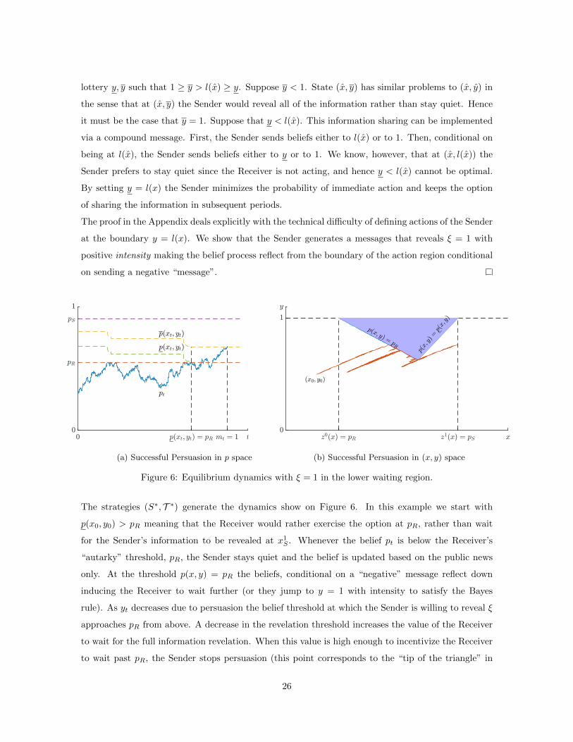
Figure 6: Equilibrium dynamics with ξ = 1 in the lower waiting region.

The strategies (S∗, T ∗) generate the dynamics show on Figure 6. In this example we start with

p(x0, y0) > pR meaning that the Receiver would rather exercise the option at pR, rather than wait

for the Sender’s information to be revealed at x1S . Whenever the belief pt is below the Receiver’s

“autarky” threshold, pR, the Sender stays quiet and the belief is updated based on the public news

only. At the threshold p(x, y) = pR the beliefs, conditional on a “negative” message reflect down

inducing the Receiver to wait further (or they jump to y = 1 with intensity to satisfy the Bayes

rule). As yt decreases due to persuasion the belief threshold at which the Sender is willing to reveal ξ

approaches pR from above. A decrease in the revelation threshold increases the value of the Receiver

to wait for the full information revelation. When this value is high enough to incentivize the Receiver

to wait past pR, the Sender stops persuasion (this point corresponds to the “tip of the triangle” in

26

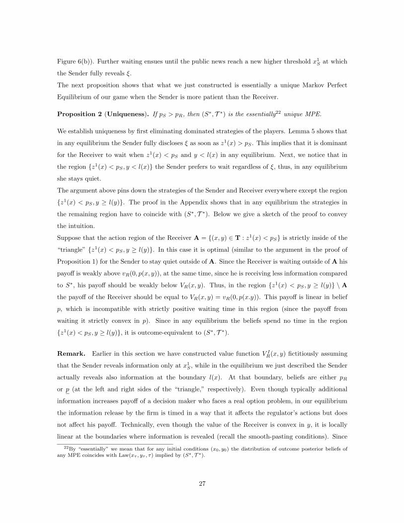
Figure 6(b)). Further waiting ensues until the public news reach a new higher threshold x1S at which

the Sender fully reveals ξ.

The next proposition shows that what we just constructed is essentially a unique Markov Perfect

Equilibrium of our game when the Sender is more patient than the Receiver.

Proposition 2 (Uniqueness). If pS > pR, then (S∗, T ∗) is the essentially22 unique MPE.

We establish uniqueness by first eliminating dominated strategies of the players. Lemma 5 shows that

in any equilibrium the Sender fully discloses ξ as soon as z1(x) > pS . This implies that it is dominant

for the Receiver to wait when z1(x) < pS and y < l(x) in any equilibrium. Next, we notice that in

the region z1(x) < pS , y < l(x) the Sender prefers to wait regardless of ξ, thus, in any equilibrium

she stays quiet.

The argument above pins down the strategies of the Sender and Receiver everywhere except the region

z1(x) < pS , y ≥ l(y). The proof in the Appendix shows that in any equilibrium the strategies in

the remaining region have to coincide with (S∗, T ∗). Below we give a sketch of the proof to convey

the intuition.

Suppose that the action region of the Receiver A = (x, y) ∈ T : z1(x) < pS is strictly inside of the

“triangle” z1(x) < pS , y ≥ l(y). In this case it is optimal (similar to the argument in the proof of

Proposition 1) for the Sender to stay quiet outside of A. Since the Receiver is waiting outside of A his

payoff is weakly above vR(0, p(x, y)), at the same time, since he is receiving less information compared

to S∗, his payoff should be weakly below VR(x, y). Thus, in the region z1(x) < pS , y ≥ l(y) \ A

the payoff of the Receiver should be equal to VR(x, y) = vR(0, p(x.y)). This payoff is linear in belief

p, which is incompatible with strictly positive waiting time in this region (since the payoff from

waiting it strictly convex in p). Since in any equilibrium the beliefs spend no time in the region

z1(x) < pS , y ≥ l(y), it is outcome-equivalent to (S∗, T ∗).

Remark. Earlier in this section we have constructed value function V IR(x, y) fictitiously assuming

that the Sender reveals information only at x1S , while in the equilibrium we just described the Sender

actually reveals also information at the boundary l(x). At that boundary, beliefs are either pR

or p (at the left and right sides of the “triangle,” respectively). Even though typically additional

information increases payoff of a decision maker who faces a real option problem, in our equilibrium

the information release by the firm is timed in a way that it affects the regulator’s actions but does

not affect his payoff. Technically, even though the value of the Receiver is convex in y, it is locally

linear at the boundaries where information is revealed (recall the smooth-pasting conditions). Since

22By “essentially” we mean that for any initial conditions (x0, y0) the distribution of outcome posterior beliefs ofany MPE coincides with Law(xτ , yτ , τ) implied by (S∗, T ∗).

27

the equilibrium information disclosure reflects beliefs only locally, it keeps the Receiver indifferent and

hence does not create any value for him.

Remark. We want to highlight two features of the equilibrium. If the prior beliefs and parameters

are such that the beliefs on the equilibrium path do not cross the l(x) “triangle” in Figure 5, then the

outcome has the compromise property we discussed. That has two consequences. First, anytime ξ = 1

is revealed, the firm does not need to be compelled to recall the drug - it is happy to do so voluntarily.

That is not true in the “pipetting region” - there upon revealing ξ = 1 the regulator decides to recall

the draft and that is against the wishes of the firm. Second, the “compromise” property implies that

the equilibrium is robust to replacing the verifiable information about ξ with cheap talk. The reason

is that at x1S the firm has aligned incentives with the regulator to reveal the truth. If the firm does

not perform self-recall past x1S , the regulator can credibly infer that ξ = 0 and stop accordingly. That

is again not true in the “pipetting” region: there if the firm is about to reveal ξ = 1, it would prefer

to mislead (at least temporarily) the regulator that ξ = 0.

4.1 Comparative Statics

We finish this section discussing some comparative statics of the equilibrium.

Comparative static on the size of the triangle. Keeping the assumption pS > pR, define

by (x∗, y∗) to be the unique solution of pR = p(x∗, y∗). Visually, point (x∗, y∗) is the lower tip

of the Receiver’s action “triangle” depicted in Figure 5. This point is important because it affects

equilibrium dynamics: arrival of public news shifts beliefs along non-intersecting curves in the (x, y)

space as shown in Figure 2. If such curve passing through the prior (x0, y0) does not intersect the

triangle, then along the equilibrium path information is revealed once and fully when xt = x1S and

the timing of the option exercise features a “compromise” property. If the initial curve crosses the

“triangle”, along the equilibrium path the Sender initially “pipets” information until either bad news

arrives revealing ξ = 1 or beliefs reach the tip of the triangle, at which point both players wait until

x1S .

Dependence on Sender’s Information Precision. The next lemma shows that the amount of

delay in equilibrium is increasing with the precision of Sender’s signal ξ.

Lemma 6. The Receiver is willing to wait longer when the Sender’s signal ξ is more precise:

∂y∗

∂z10> 0,

∂y∗

∂z00< 0.

28

As z10 goes up Sender’s signal ξ becomes more precise about the state θ = 1. As a result, the

information revelation threshold x1S decreases since, conditional on ξ = 1, the Sender is requires less

positive public news to reach a belief pS . A lower x1S , in turn, corresponds to a smaller Receiver’s

cost of waiting for the discrete information revelation. At (x∗, y∗) the Receiver is exactly indifferent

between acting immediately and waiting for x1S . As z10 increases, Receiver’s option value to wait at

(x∗, y∗) increasing leading him to prefer waiting rather than acting. This shifts the tip of the triangle

up.

As z00 decreases, Sender’s signal ξ becomes more precise about the state θ = 0. This has no effect

on her incentives to reveal information at x1S . However it makes the information disclosed that is

discretely disclosed of higher quality. Because Receiver’s value function is strictly convex in beliefs,

this increases the payoff of waiting for the Receiver. Graphically, as z00 decreases, the tip of the triangle

(x∗, y∗) increases.

Level of Disagreement. In our model disagreement between the Sender and Receiver is summa-

rized by the distance between pR and pS , the no-additional-information thresholds.

Lemma 7. As the disagreement of preferences increases the Receiver is willing to wait less before

acting:∂y∗

∂pS< 0

The intuition is simply that a higher pS implies a higher x1S since the firm is going to wait longer to

self-recall the drug. The Receiver now has to wait longer for the discrete revelation of information.

Naturally, this decreases the value of waiting to learn ξ and expands the range of beliefs for which the

Receiver is willing to exercise the option in equilibrium.

5 Impatient Sender pS ≤ pR

We now turn to the opposite case, when it is the Receiver who would like to exercise the real option

sooner than the Sender, which is captured by the assumption pS ≤ pR. As we discussed above, that

can correspond to a situation where an agent works for a principal and they learn jointly from public

news about a potential project the agent would like to start. The conflict of interest is that either

because the project gives the agent private benefits or that the agent does not fully internalize the

fixed cost of starting it, she would like to start her project sooner than the principal.

29

5.1 Immediate Revelation Equilibrium

Our first result is that there exists a MPE in which the Sender reveals information immediately, after

every history.

Proposition 3. There exists a MPE in which signal ξ is fully revealed by the Sender after all histories.

In such equilibrium the Receiver achieves the first best by adopting a very “strong bargaining position”:

he threatens not to exercise the option until either all information about ξ is revealed, or the public

news render additional information that could be obtained by the Sender irrelevant, i.e. z0(x) ≥ pR.

Given the equilibrium strategy of the Sender such threat is credible, since waiting for the information

to be released at the next instance is costless in continuous time. The Sender faces a tough choice:

either to reveal ξ immediately, or to wait until z0(x) = pR; any partial information revelation does

not affect the timing of option exercise. If the Sender reveals ξ, then the option is exercised either at

z1(x) = pR (if ξ = 1) or at z0(x) = pR (if ξ = 0). Since she prefers the option to be exercised earlier

and z0(x) < z1(x) the Sender is better off revealing ξ at time 0.

Note that the same reasoning does not apply to the previous case of a patient Sender. In that case, if

the Receiver could commit to a strategy “I stop in the next second unless you reveal all information

about ξ,” the Sender’s best response would be to reveal such additional information. But that threat

is not credible: if the Sender does not provide information, it is not credible for the Receiver to stop

before beliefs reach pR.

In the next sections we show that under some parametric assumptions this is the unique Markov

Perfect Equilibrium and that in general, Receiver’s decision threshold is always higher than absent

persuasion, which implies that in these cases the Sender is worse off as a result of having access to

information about ξ.

5.2 Equilibrium Uniqueness

First we show that in any Recommendation Equilibrium if mt = 1 is an informative message, then

it fully reveals ξ = 1. As a consequence, in equilibrium the option is exercised either when yt = 1 or

after a period of no persuasion.

Lemma 8. In any Recommendation Equilibrium if Pt(ξ = 1|mt = 1) > Pt(ξ = 1|mt = 0) then

Pt(ξ = 1|mt = 1) = 1.

The above lemma highlights the impact of public news on the equilibrium behavior. The proof

constructs an unraveling argument that we illustrate with an example in which signal ξ is perfectly

informative of θ. Suppose the Receiver’s strategy is to wait when belief is below some threshold p and

30

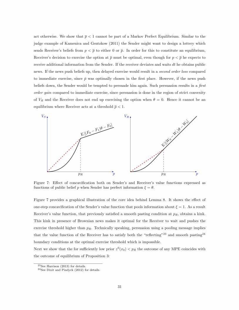
act otherwise. We show that p < 1 cannot be part of a Markov Perfect Equilibrium. Similar to the

judge example of Kamenica and Gentzkow (2011) the Sender might want to design a lottery which

sends Receiver’s beliefs from p < p to either 0 or p. In order for this to constitute an equilibrium,

Receiver’s decision to exercise the option at p must be optimal, even though for p < p he expects to

receive additional information from the Sender. If the receiver deviates and waits dt he obtains public

news. If the news push beliefs up, then delayed exercise would result in a second order loss compared

to immediate exercise, since p was optimally chosen in the first place. However, if the news push

beliefs down, the Sender would be tempted to persuade him again. Such persuasion results in a first

order gain compared to immediate exercise, since persuasion is done in the region of strict convexity

of VR and the Receiver does not end up exercising the option when θ = 0. Hence it cannot be an

equilibrium where Receiver acts at a threshold p < 1.

p

VS

E [(F0− F1)θ

− F0]

pR p

VR

E[(W

0−W

1)θ−W

0]

pR

Figure 7: Effect of concavification both on Sender’s and Receiver’s value functions expressed asfunctions of public belief p when Sender has perfect information ξ = θ.

Figure 7 provides a graphical illustration of the core idea behind Lemma 8. It shows the effect of

one-step concavification of the Sender’s value function that pools information about ξ = 1. As a result

Receiver’s value function, that previously satisfied a smooth pasting condition at pR, obtains a kink.

This kink in presence of Brownian news makes it optimal for the Receiver to wait and pushes the

exercise threshold higher than pR. Technically speaking, persuasion using a pooling message implies

that the value function of the Receiver has to satisfy both the “reflecting”23 and smooth pasting24

boundary conditions at the optimal exercise threshold which is impossible.

Next we show that the for sufficiently low prior z0(x0) < pR the outcome of any MPE coincides with

the outcome of equilibrium of Proposition 3:

23See Harrison (2013) for details.24See Dixit and Pindyck (2012) for details.

31

Proposition 4. If z1(x0) ≤ pR, then the equilibrium outcome of Proposition 3 is essentially unique.

Moreover, regardless of z1(x0) in any MPE (T ∗,H∗) the stopping set T∗ is strictly inside of the

autarky stopping set (x, y) : p(x, y) ≥ pR.

We prove the first part of the proposition by showing that given the initial condition z1(x0) ≤ pR in

any MPE the option is exercised only when ξ is fully revealed. Since the Sender prefers early exercise

immediate revelation of ξ guarantees that the Receiver stops exactly when z1(x) = pR or z0(x) = pR.

To see why the second part of Proposition 4 holds, one has to notice that full revelation of ξ at x1R

such that z1(x1R) = pR creates additional option value for the Receiver when the beliefs approach this

threshold from above. Hence he will no longer prefer to stop at p(x, y) = pR because his value from

waiting is now strictly higher.

Suppose now that Receiver’s prior beliefs at t = 0 are pR and the Sender would prefer him to exercise

the option. Then, absent persuasion, this would be the outcome of the game. The Receiver, however,

expects the Sender to reveal more information when public beliefs drop. Hence he will no longer

wish to exercise the option at pR. This hurts the value of the Sender since, under some parameters,

unconditional exercise would result in a first best outcome had they started with sufficiently high

beliefs.

Corollary 1. Suppose V NIS (z0(x0)) < (F0 − F1)z0(x0)− F1 at t = 0 and y0 ∈ (0, 1). If initial beliefs

are p0 = pR then Sender’s value in any MPE is strictly lower than his value if the Receiver acted just

based on public news.

Proof. Absent persuasion the Receiver would have exercised the real option at pR which would have

been the best outcome for the Sender. Due to persuasion, however, Receiver’s decision threshold is

strictly higher than pR.

5.3 Special Case: z0(x) ≡ 0

In this section we prove the uniqueness of the equilibrium for a special case when the Receiver can

obtain a perfect information about θ = 0:

Proposition 5. Suppose z0(x) ≡ 0 then the equilibrium of Proposition 3 is essentially unique.

When z0 = 0 and the Sender learns that ξ = 0, then, the Sender knows that the state of nature is

θ = 0. If F0 < 0, the Sender does not wish to exercise the option. In that case it is a dominant

strategy for her to disclose all of information immediately: if ξ = 0 she gets her preferred action and

when ξ = 1 she gets the Receiver speed up exercise as much as possible.

If, however, she prefers pooling (F0 > 0), then for any interior decision threshold y = l(x) of the

Receiver there is always a point (x∗, y∗), such that she always prefers to send a pooling message to

32

induce action. Given such a best response of the Sender to threshold l(·) we have a contradiction with

Lemma 8. The Receiver will expect such a pooling message at x∗ and his threshold will be strictly

higher than l(x∗). Hence a threshold 0 < l(x) < 1 cannot be part of any Markov Perfect Equilibrium.

Remark. This is a stark difference to a result of persuasion with commitment. It can be shown

that when z00 = 0 the Sender engages in immediate persuasion by doing a lottery between z00 and

min(z10 , pR).

6 Conclusion

In this paper we study a dynamic Bayesian persuasion game in which the Sender and the Receiver

learn jointly about the state of the nature from a stream of public news. The Sender can acquire

additional informative signals; she decides what signals and when to acquire but has no long-term

commitment power. The Receiver, upon observing public news and additional information generated

by the Sender, decides when to take an irreversible action (exercise a real option) and also have no

commitment power to future stopping decisions. This analysis is motivated by many problems where

one agent has decision power over a real option (e.g. a regulator) and another agent, with partially

misaligned preferences (e.g. a medical device supplier), can acquire additional information to influence

the decision-maker.

We show that there exists a unique Markov Perfect equilibrium and characterize equilibrium dynamics

of information provision when the Sender prefers later exercise. If misalignment of incentives is small,

in equilibrium the Sender acquires information once and it is fully revealing. Anticipating a discrete

information disclosure, the Receiver is willing to wait past a belief threshold at which he would stop

with only public news. Depending on the information disclosed, the option is exercised at either the

Senders optimal threshold, in which case the Receiver ex-post regrets waiting for too long, or at the

Receivers optimal threshold. Thus, the timing of option exercise features a compromise property. If

misalignment of incentives is large, Sender [initially] resorts to pipetting of information over time.

Pipetting results in belief process that either reflects from the action threshold of the Receiver or

discretely jumps, triggering immediate exercise of the option. Such information provision changes

the timing of the option exercise and allows the Sender to reach the compromise region with positive

probability, however, it does not generate any value for the Receiver.

When the Sender prefers earlier exercise her inability to stop persuading undermines her ability to

speed up the option exercise time. We show that there always exists an equilibrium in which the Sender

discloses all information at time zero, and in several cases this equilibrium is unique. In contrast to

the static environment of Kamenica and Gentzkow (2011) pooling of information unravels due to the

33

option of the Receiver to wait and obtain more information from the Sender in the immediate future.

Moreover, we show that for some parameter values the Sender is worse off as a result of having access

to additional information in all Markov equilibria.

34

Appendix

Proof of Lemma 1. The most extreme beliefs that the sender can induce at any time t can be

expressed as a function of initial conditions and xt:

zit = Pt(θ = 1|ξ = i) =zi0e

xt

zi0ext + (1− zi0)

= zi(xt)

The triplet (pt, q0t , q

1t ) maps naturally into (z0(xt), z

1(xt), yt) via

pt = yt · z1(xt) + (1− yt) · z0(xt),

q1t =z1(xt)ytpt,

q0t =(1− z1(xt))yt

1− pt.

Public news and persuasion are subsequently captured by the pair (xt, yt).

Proof of Lemma 2 . Suppose VS(x, y) corresponds to Sender’s equilibrium value function. First, it

must satisfy

VS(x, y) = cavyVS(x, y) (A.1)

where x is taken as constant and the concavification operator is applied only w.r.t. y. If (A.1) did

not hold for any y, then the Sender can improve his value by sending a single informative signal and

then returning to the original strategy. This proves global concavity in y. It also implies continuity

in y.

Second, the Sender has the option to choose the time when he starts persuading the receiver:

VS(x, y) = supκ

E(x,y)

[e−rτ · VS(xτ∧κ, yτ∧κ)

](A.2)

where

τ = inft : (xt, yt) ∈ T ∗

Moreover because the simple solution of κ = 0 achieves the optimum, we have

VS(x, y) = maxκ

E(x,y)

[e−rτ · VS(xτ∧κ), yτ∧κ

]The solution must be continuous along the path of no persuasion (x, y(x)). Because it is continuous

in y it implies that it is continuous in x. Suppose y ∈ E(x). It implies that there is no action and no

persuasion being conducted by the Sender (because of strict concavity).

35

Suppose that y ∈ E(x). This implies that in the vicinity of (x, y) there is no persuasion. Hence for

κ = inft : yt /∈ E(xt)

we have

VS(x, y) = E(x,y)

[e−rκ∧τ · VS(xτ∧κ), yτ∧κ

]Hence VS must satisfy (14).

Proof of Lemma 3. First we show a property of the Sender’s best response to any strategy. Suppose

yL0 < yH0 and yL0 , yH0 ∈ E(x). There exists an information sharing strategy of the Sender delivering

him his equilibrium value such that yHt ≥ yLt . From the contrary define (we can define it with some

small gap ∆ just as way to make it a non-strict inequality)

κ = inft < κ : Y Lt > Y Ht

Denote the random set E = E(xκ). Then

limε→0,ε>0

Y Lκ−ε = Y Lκ− /∈ E

Process Y Lt is continuous when Y Lt ∈ E(xt). Suppose that Y Hκ− ∈ E. Then according to the Sender’s

strategy it will be the case that Y Lκ ≤ Y Hκ and we have a contradiction. Hence it must be the case

that Y Hκ− /∈ E. This implies that both along both belief paths L and H in state xτ the Sender creates

signals. It is clear that we must focus on the case when ∀y ∈ [Y Lκ−, YHκ−] we have y /∈ E. Otherwise

Sender’s signals would not alter the ranking of beliefs.

The lottery is going to be between two points y and y. The probability that message y is sent by the

Sender is given by

αL =Y Lκ− − yy − y

αH =Y Hκ− − yy − y

The Sender can implement his strategy by delivering two messages. One that sends messages from

Y L to y and Y H . It does not hurt the Sender and the Receiver’s continuation value does not change.

Hence Y Ht ≥ Y Lt . This implies that if the Receiver has a signal about y0 at t = 0, this leads to a

lottery over all subsequent paths. Because he can ignore this information when making the decision,

this leads to convexity in his value function in equilibrium.

36

It is not obvious that the above constitutes a threshold rule. Suppose VR(x, 1) > vR(0, z1(x)). This

implies that the receiver prefers waiting even if all of the information is revealed. The Receiver

solves his real option problem and the above is equivalent to z1(x) < pR. In this case z1(x)y +

z0(x)(1 − y) < pR for y < 1 as well. Hence VR(x, y) > vR(0, z1(x)y + z0(x)(1 − y)) for y ∈ [0, 1]. If

VR(x, 1) ≤ vR(0, z1(x)), then l(x) = supy : VR(x, y) > vR(0, z1(x)y + z0(x)(1− y)) is well defined

and

VR(x, y) > vR(0, z1(x)y + z0(x)(1− y)) for y < l(x),

VR(x, y) = vR(0, z1(x)y + z0(x)(1− y)) for y ≥ l(x).

Clearly the strategy of the Receiver “wait if yt ≥ l(xt) and act otherwise” is a best response, however,

there are many others since in the region y > l(x) the Receiver is indifferent between acting and not.

We now show that in any equilibrium the beliefs spend measure zero time in the region 1 > y > l(x),

thus, it is without loss of generality to consider a threshold best response T.

Suppose the contrary, and consider a given (x0, y0) with y0 > l(x0) and T (x0, y0) = 0. Define E to

be the set of pairs (x, y) that correspond to the extreme point of VS , i.e.

E = (x, y) : y ∈ E(x).

If (x0, y0) ∈ int(E), then starting at (x0, y0) a positive waiting ensues with only the public news

arriving. In this region VS is linear in p but has to satisfy a second order ODE and be strictly convex

- a contradiction. If (x0, y0) /∈ intE, then y0 ∈ [y(x0, y0), y(x0, y0)]. Notice that y(x0, y0) ≤ l(x0) oth-

erwise, there would be some positive quiet time starting at some (x0, y′0) with y′0 ∈ (l(x0), y(x0, y0))

which we have shown to be a contradiction. Similarly y(x0, y0) = 1, otherwise, there would is some

quite time starting at some (x0, y′0) with y′0 > y(x0, y0). Thus, starting at (x0, y0) the sender imme-

diately sends beliefs out of the region 1 > y > l(x), and we can put T(x0, y0) = 1 without changing

the outcome of the equilibrium.

Proof of Lemma 4. In the existing equilibrium (T ∗,H) process (xt, yt) is Markov. Define

mt = maxs≤t

T(xs, ys)

Define

τ = inft : mt = 1

37

The new belief process is given by

yt = P(ξ = 1|xt,mt = 0)

It satisfies the SDE

dyt = (z1(xt) − z0(xt))yt(1 − yt)φdBt + (y(t, xt,mt = 1) − yt)(dNt − λ(t, xt,mt = 0) dt)

This implies process (xt, yt, t) is Markov. This equilibrium is not MPE in beliefs yet because of the

time dependency of the intensity λ(t, xt,mt = 0). Define the corresponding value function VS(t, y, x).

Suppose

maxtVS(t, y, x) > min

tVS(t, y, x)

Then the Sender has a profitable deviation in the original equilibrium. Hence VS(t, y, x) = VS(0, y, x).

Define the optimal strategy as

λ∗(x,mt = 0) = λ(0, x,m = 0)

This leads to the same expected value for the Sender and a Markov recommendation strategy.

Proof of Lemma 5. If ξ(ω) = 1, then disclosing it results in immediate exercise of the option by

the receiver, which is the first best outcome for the sender conditional on ξ(ω) = 1. Any delay in such

a state ω decreases sender’s pay-off conditional on ξ = 1.

Consider the case with ξ(ω) = 0. Let pτ denote the equilibrium level of beliefs about θ at the

moment of option exercise. It must be that pτ ≥ P(θ = 1|pτ , ξ = 0). Without loss, this inequality

is strict in some states of the world. In those states revealing ξ = 0 at t = τ lowers the belief

of the receiver and weakly delays option exercise. If P(θ = 1|pτ , ξ = 0) > pR, then the option is

exercised by the receiver regardless of the sender’s information, hence, revealing is weakly optimal.

If P(θ = 1|pτ , ξ = 0) ≤ pR < pS , delaying option exercise in this region improves sender’s conditional

payoff pay-off – a contradiction. Thus, pτ = P(θ = 1|pτ , ξ = 0) i.e. negative signal ξ = 0 is fully

disclosed in any equilibrium. Revealing ξ = 0 at t = 0 path-by-path results in the same exercise time

τ and induces the same pay-off to both receiver and the sender, conditional on ξ = 0.

Lemma 9. For any fixed x there exists yH(x) such that V NIR (x, y) ≥ V IR(x, y) when y ≥ yH(x).

Proof of Lemma 9. It is sufficient to show that

∂

∂y

[V IR(x, y)− V NIR (x, y)

]∣∣∣p(x,y)=p

= 0.

38

Consider a function f that solves

rRf(p) =1

2φ2p2(1− p)2f ′′(p) p ∈ (a, b)

f(a) = vR(0, a)

f(b) = y · vR(0, pS) + (1− y)V NIR (x, 0)

To show the dependence on the boundary conditions can write f(p; a, b). Notice that f(p; p, p) coin-

cides with V IR as a function of p in the relevant region. Recall that

∂

∂pf(p; p, p) =

∂

∂pvR(0, p).

Next increase y to y+dy, and consider the new triplet p′ = p+dp(y) p′ = p+dp(y) and p′ = p+dp(y).

We can check whether the smoothpasting condition holds and the new boundary p′:

∂

∂pf(p′; p′, p′) =

∂

∂p

(f(p; p, p) +

∂

∂pf(p; p, p)dp(y) +

∂

∂pf(p; p, p)dp(y) +

∂

∂pf(p; p, p)dp(y)

)=

∂

∂p

(f(p; p, p) +

∂

∂pf(p; p, p)dp(y)

)<

∂

∂pf(p; p, p)

=∂

∂pvR(0, p)

where the second equality holds since

∂2

∂p2f(p; p, p) = − ∂2

∂p∂pf(p; p, p) =

2rRf(p)

φ2p2(1− p)2.

Thus, the optimal exercise threshold p(y) increases faster than the current belief p(y) and an increase

in y keeps the beliefs in the linear part of V IR = V NIR .

Explicit Construction of the Reflected Process First, define yt to be the naive posterior about

ξ that is updated based only on public news, i.e.

yt = P(ξ = 1 |Xt) = g(xt;x0, y0).

39

For any belief process y induced by the Sender define a(xt, yt) to be

a(xt, yt) = g(x0;xt, yt). (A.3)

Intuitively, a(xt, yt) is the belief about ξ that is updated only on the information generated by the

sender above and beyond public news. Clearly the state of the game can be described by a pair (x, a)

instead of (x, y) and it is natural to think of a as a pure control variable of the Sender since it is not

confounded by the public news. Given a path xt define a∗t to be

a∗t = min[y0, inf

s≤tg(x0;xs, l(xs))

]. (A.4)

Given the process a∗ we now define the belief y simply as

y∗t = g(xt;x0, a∗t ). (A.5)

Lemma 10. Process a∗t is the unique process such that (xt, y∗t ) /∈ T and it changes if and only if

y∗t = l(xt).

Proof. Step 1: reflection. Suppose there exists some realization ω ∈ Ω and time t such that

y∗t (ω) > l(xt(ω)). This implies that a(xt(ω), y∗t (ω)) > a∗t (ω) and gives rise to a contradiction

y∗t (ω) ≡ g(xt(ω);x0, a(xt(ω), y∗t (ω))) > g(xt(ω);x0, a∗t (ω)) = y∗t (ω).

Moreover, notice that y∗t satisfies

y∗t =

∫ t

0

[(z1(xs)− z0(xs))y

∗s (1− y∗s )φdBs +

∂

∂yg(xs;x0, a

∗s)das

].

Step 2: uniqueness. Suppose there is an alternative process yt such that in the region (x, y) /∈ T it

behaves like the standard belief process, while (xt, yt) /∈ T. The new process (xt, yt) corresponds to

the process at given by

at = min[y0, inf

s≤tg(x0;xs, ys)

]Then for the same paths we must have a∗t ≥ at. This implies that y∗t ≥ yt. It is possible to show that

the Sender’s payoff is greater if path by path process a∗t is greater.

Proof of Proposition 2. Define l(x) to be the threshold in the already constructed equilibrium

such that the receiver stops when y > l(x). Suppose there exists an alternative equilibrium with

l(x) 6= l(x). The following properties apply:

40

(i) The receiver never finds it incentive compatible to stop before l(x). This implies that l(x) ≥ l(x).

(ii) The sender does not reveal any information for y ≤ l(x). Otherwise he can delay sending the

same message.

Denote by V (x, y) the value obtained by the receiver in the alternative equilibrium. Then V (x, y) ≤

V (x, y). Otherwise we can add the external news process from the original equilibrium and implement

the value function V (x, y) but the receiver will have strictly more information. On the other hand,

in the original equilibrium belief reflection does not add value. This implies that V (x, y) ≥ V (x, y).

This keeps the possibility that V (x, y) = V (x, y).

Note that for y < l(x)+l(x)2 there is no persuasion in the alternative equilibrium. Convexity of the

ODE solution in p in the waiting for these y and the result that V (x, y) = V (x, y) once y < l(x)

and y > l(x) it implies that V (x, y) < V (x, y) in that region. This contradicts V (x, y) = V (x, y) for

y < l(x).

Proof of Lemma 6 . Holding y fixed, when z1 is increased two things happen. First, the Sender

discloses information sooner. Second, Receiver’s belief about the fundamental p = yz1 +(1−y)z0 also

increases. At the point (x∗, y∗) the Receiver is indifferent between acting and waiting for the discrete

piece of news

V NIR (x∗, y∗) = V IR(x∗, y∗)

Moreover these functions just depend on p

V NIR (x∗, y∗) = fNIR (y∗z1(x∗) + (1− y∗)z0(x∗))

V IR(x∗, y∗) = f IR(y∗z1(x∗) + (1− y∗)z0(x∗))

Note thatdfI

R

dp (pR) ≥ dfIR

dp (pR) when at z1(xτ ) = pS the Sender reveals everything. Sensitivity of

V NIR (x, y) with respect to z1 is equal to y at the smooth pasting point. Now consider the representation

of V IR.

V IR(x, y) = fR(pS(z1), yz1 + (1− y)z0)

The Receiver strictly prefers observing the signal z1 earlier, rather than later. Hence

∂fR∂pS

< 0

Then∂V IR(x∗, y∗)

∂z1=∂fR∂pS

∂pS∂z1

+∂fR∂p· y∗ > y∗ =

∂V NIR

∂z1(x∗, y∗)

Hence when z1 is increased, V IR increases by more than V NIR , and which implies that l(x∗) increases.

41

Next, suppose z0 decreases. This implies that conditional on ξ = 0 the Sender has more precise

information. The value function of the Receiver upon obtaining this information is

V IR(x, y) = E[e−rτS (yτS ((W 0 −W 1)pS −W 0) + (1− yτS )(V NIR (z0τS )))

]The derivative wrt z0 is given by

V IR(x, y) = (1− yτS ) · ∂fNIR

∂p· (z0τS )E

[e−rτS

]< 1− y

Hence when z0 is decreased the value of V IR decreases at a smaller rate than V NIR . This implies that

when z0 declines, l(x∗) has to increase.

Proof of Proposition 3. Consider the following pair of Markov strategies:

T ∗: Receiver acts if and only if

vR(0, z1(x)y + z0(x)(1− y)) ≥ y · V NIR (1, x) + (1− y) · V NIR (0, x)

H∗: Sender reveals ξ after every history.

Now we need to check that these strategies are a best response to one another after every history.

Receiver’s best response is easy: if he believes a positive amount of information is about to be revealed

the next instance he chooses to wait. The only case when he does not is when this information is

irrelevant for decision making z0 ≥ pR. In that region, however, the Sender is indifferent between

disclosing information and not since it does not affect option exercise.

To compute the Sender’s best response we must show that if all information must be revealed for the

action to take place, she chooses to reveal it immediately (when z0 ≥ pR the information is irrelevant

for Sender’s decision as well and she might as well reveal everything). Denote by τ the moment when

ξ is fully revealed. Then

piτ = ziτ i = 0, 1

The Sender solves

maxτ

E

[e−rτ · yτ · V NIS

(z1(xτ )

)+ e−rτ · (1− yτ ) · V NIS

(z0(xτ )

)]

In order for immediate disclosure to be the best response, the solution to the above stopping problem

must be τ∗ = 0. We can simplify by aligning incentives of the Sender conditional on ξ. Type 1 Sender

42

prefers immediate disclosure after any history. Type 0 Sender also prefers immediate disclosure since

the Receiver will not act at a threshold lower than pR after any history.

Proof of Lemma 8. Fix the strategy of the Sender. It specified a public beliefs process pt. It is a

combination of public news and Sender’s messages. The belief pt can be decomposed into (xt, yt). In

the region where the Sender chooses to send an informative message, she sends a signal leading beliefs

in yt to be either yH(x) and yL(x).

VR(x, y) =y − yL(x)

yH(x)− yL(x)· VR(x, yH(x)) +

yH(x)− yyH(x)− yL(x)

· VR (x, yL(x))

In particular

VR(x, yH(x)) = vR(0, yH(x)z1(x) + (1− yH(x))z0(x)

)The optimal stopping problem of the receiver implies that ∀(x, y)

VR(x, y) ≥ vR(0, z1(x)y + z0(x)(1− y))

Function z1(x)y + z0(x)(1− y) is increasing in x. The above inequality implies

limε→0

VR(x, yH(x))− VR(x− ε, yH(x))

ε≤ dz1(x)

dx· yH(x) +

dz0(x)

dx· (1− yH(x))

limε→0

VR(x+ ε, yH(x))− VR(x, yH(x))

ε≥ dz1(x)

dx· yH(x) +

dz0(x)

dx· (1− yH(x))

If the above is not true, then there exists x∗ and y∗ = yH(x∗) such that

VR(x∗, y∗) < vR(0, z1(x∗)y∗ + z0(x∗) · (1− y∗))

which contradicts the optimal stopping of the Receiver. The derivative with respect to y is given by

∂VR∂y

(x, y) =1

yH(x)− yL(x)·(vR(0, z1(x)yH(x) + z0(x)(1− yH(x))

)− VR(x, yL(x))

)= −

VR(x, yL(x))− vR(0, z1(x)yL(x)− z0(x)(1− yL(x))

)yH(x)− yL(x)

+ (z1(x)− z0(x)) · (W 0 −W 1)

< (z1(x)− z0(x)) · (W 1 −W 0)

The calculations above show that VR(x, y) has a non-negative kink in x and strictly positive kink in y

at every point of (x, yH(x)). Consider one such point (x, y) = (x, yH(x)) with a corresponding belief

43

p = P(θ = 1|x, y) and suppose that y < 1. Then the function fS(p) defined as

fR(p) = VR(x(p), y(p)) with x′(p), y′(p) > 0

has a positive kink at p.

Proof of Proposition 4 . Recall that for all p(x, y) < pR it is dominant strategy for the receiver to

wait, thus, without loss of generality, we can assume that for all x such that z1(x) < pR sender does

not reveal any information.

Define

τ = inft : yt ≥ yH(xt) or yt /∈ E(xt)

This is the first moment where there will be either action of information sharing. We know that

pt = p(xt, y(xt)) evolves according to the public news process for t ≤ τ and no action is undertaken

by the Receiver.

Suppose yτ ≥ yH(xτ ). Since the sender is not disclosing any information up to (and including) the

time τ it has to be that p(xτ , yτ ) = pR. Thus, VS(x0, y0) = V NIS (p(x0, y0)). If the sender fully reveals

information at time 0 (or, pay-off equivalently at time τ ′ = inft > 0 : z1(xt) ≥ pR) her pay-off is

y0VNIS (z1(x0)) + (1− y0)V NIS (z0(x0)) > V NIS (p(x0, y0)).

The inequality holds due to strict convexity of V NIS (p) for all p ≤ pR.

Profitable deviation outlined in the previous paragraph implies that yτ < yH(xτ ) for all (y0, x0) such

that z1(x0) < pR. Consider

y = infy0∈[0,1]

yτ = yτ (x0, y0),

and suppose that y > 0. Then there exists y0 small enough that path of (xt, yt) updated only on

public news satisfies y(xt) ∈ E(xt) for all t ≥ 0, i.e., the sender does not reveal any information along

this path. This can not be the case, since the receiver would act at p(xt, y(xt)) = pR which contradicts

yτ < yH(xτ ). Thus, y = 0, implying that for all (x0, y0) with z1(x0) < pR in any MPE the action is

taken only after ξ is fully revealed and

VS(x0, y0) ≤ y0V NIS (z1(x0)) + (1− y0)V NIS (z0(x0)).

44

Clearly, revealing information at t = 0 (or at τ ′) generates

VS(x0, y0) = y0VNIS (z1(x0)) + (1− y0)V NIS (z0(x0))

and achieves the upper bound on the equilibrium value function of the Sender.

Proof of Proposition 5 . After any history Sender’s value function cannot exceed:

p

pR· ((F0 − F1)pR − F0)

Suppose z1(x) = pR. Sender’s beliefs are given by p = y ·z1(x) = pR. Then full information revelation

implies

y · ((F0 − F1)pR − F0) =p

pR· ((F0 − F1)pR − F0)

For a given equilibrium payoff VS(x, y) along the particular path of beliefs define W (p) to be the upper

bound. It is constructed as follows. Given the path of (x, y) between the waiting and the persuasion

region, denote by p the first time when the Sender sends the message m = act = ξ = 1. At p

beliefs reach Receiver’s decision threshold and the latter acts. Then

VS(x, y) ≤p

pR· p− pp− p

· ((F0 − F1)pR − F0) +p− pp− p

· ((F0 − F1)p− F0) = W (p)

where, to the benefit of the Sender, Receiver is willing to act at pR when public beliefs reach p along

this trajectory.

For a given p define by u(p) the lowest current belief at which the Receiver is willing to act. This

is coming from the threshold strategy of the Receiver in the (x, y) space – depending on the current

level of p the persuasion threshold will be different. Compare W (p) with immediate persuasion. The

value from the latter is

w(p) =p

u(p)· ((F0 − F1)u(p)− F0) = (F0 − F1)p− F0

p

u(p)

At p = p by definition u(p) = p and hence w(p) = W (p). I show that W ′(p) > w(p) implying that for

p < p it is better to persuade immediately, rather than wait.

45

[−p

pR· ((F0 − F1)pR − F0) · 1

p− p+

1

p− p· ((F0 − F1)p− F0)

]vs.

[F0 − F1 − F0 ·

1

u(p)+ F0

p

u(p)2u′(p)

]F0

p

pR· 1

p− p− F0 ·

1

p− pvs. − F0 ·

1

p

p

pR− 1 vs. −

p− p

pp

pRvs.

p

p

p > pR

For the inequalities above to hold it is sufficient that u′(p) < 0. Hence locally around p immediate

persuasion dominates the upper bound on the value that the Sender can obtain if she delays persuasion.

Q.E.D.

46

References

Viral V. Acharya, Peter DeMarzo, and Ilan Kremer. Endogenous information flows and the clustering

of announcements. The American Economic Review, 101(7):2955–2979, 2011.

Ricardo Alonso and Odilon Camara. Persuading skeptics and reaffirming believers. mimeo.

Robert J. Aumann and Michael Maschler. Repeated games with incomplete information. MIT press,

Cambridge University Press, 1995.

Isabelle Brocas and Juan D Carrillo. Influence through ignorance. The RAND Journal of Economics,

38(4):931–947, 2007.

Brendan Daley and Brett Green. Waiting for news in the market for lemons. Econometrica, 80(4):

1433–1504, 2012.

Robert K Dixit and Robert S Pindyck. Investment under Uncertainty. Princeton University Press,

2012.

Jeffrey C. Ely. Beeps. mimeo, 2015.

Peter Eso and Yuk-Fai Fong. Wait and see: A theory of communication over time. mimeo, 2010.

Peter Eso, Balazs Szentes, et al. The one who controls the information appropriates its rents. mimeo.

Matthew Gentzkow and Emir Kamenica. Competition in persuasion. mimeo, 2016.

Steven R Grenadier, Andrey Malenko, and Nadya Malenko. Timing decisions in organizations: Com-

munication and authority in a dynamic environment. mimeo, 2015.

Faruk Gul and Wolfgang Pesendorfer. The war of information. The Review of Economic Studies, 79

(2):707–734, 2012.

Yingni Guo. Dynamic delegation of experimentation. mimeo, 2014.

Ilan Guttman, Ilan Kremer, and Andrzej Skrzypacz. Not only what but also when: A theory of

dynamic voluntary disclosure. The American Economic Review, 104(8):2400–2420, 2014.

J Michael Harrison. Brownian Models of Performance and Control. Cambridge University Press,

2013.

Emir Kamenica and Matthew Gentzkow. Bayesian persuasion. American Economic Review, 101(6):

2590–2615, 2011.

47

Aaron M. Kolb. Reputation and strategic adoption. mimeo, 2015.

Ilan Kremer and Andrzej Skrzypacz. Dynamic signaling and market breakdown. Journal of Economic

Theory, 133(1):58–82, 2007.

Erik Madsen. Optimal project termination with an informed agent. mimeo, 2015.

George J Mailath and Larry Samuelson. Repeated games and reputations, volume 2. Oxford university

press Oxford, 2006.

Roger B. Myerson. Multistage games with communication. Econometrica, 54(2):323–358, 1986.

David Pollard. A user’s guide to measure theoretic probability, volume 8. Cambridge University Press,

2002.

Jerome Renault, Eilon Solan, and Nicolas Vieille. Optimal dynamic information provision. arXiv

preprint arXiv:1407.5649, 2014.

Yuliy Sannikov. Games with imperfectly observable actions in continuous time. Econometrica, 75(5):

1285–1329, 2007.

Leo Simon and Maxwell Stinchcombe. Extensive form games in continuous time: Pure strategies.

Econometrica, 57(5):1171–1214, 1989.

Alex Smolin. Optimal feedback design. mimeo, 2015.

48