Personalized Treatment Selection Based on

Randomized Clinical Trials

Tianxi Cai Department of Biostatistics

Harvard School of Public Health

Outline

  Motivation

  A systematic approach to separating subpopulations with differential treatment benefit in the absence of correct models

  Remarks   Evaluation of the system   Efficiency augmentation

Motivating Example AIDS Clinical Trial ACTG320

 Study Objective: to compare the efficacy of   3-drug combination therapy: Indinarvir+Zidovudine/Stavudine+Lamivudine   2-drug alternatives: Zidovudine/Stavudine + Lamivudine

 Study population: HIV infected patients with CD4 ≤ 200 and at least three months of prior zidovudine therapy   1156 patients randomized: 577 received 3-drug; 579 received 2-drug

 Study conclusion: 3-drug combination therapy was more effective compared to the 2-drug alternatives

 Question: 3-drug therapy beneficial to all subjects?

Age CD4wk 0

log10RNAwk 0

Predictor Z 2-drug

3-drug

Treatment Benefit Of 3 drug (vs 2 drug) | Z

Age: 12 CD4： 170 log10RNA: 3.00

Age: 41 CD4: 10 log10RNA: 5.69

Likely to benefit from the 3-drug? How much benefit would there be?

No two drug Treatment Benefit : 0 units of CD4 ↑

Yes three drug Treatment Benefit : 500 units of CD4 ↑

Outcome Y Change in CD4 from week 0 to 24

Background and Motivation

  Treatment × covariate interactions

  Testing for h(Z; β) = 0   Helpful for identifying Z that may affect treatment benefit

  Estimation of h(Z, β)   Robust estimators of may be obtained for certain special cases (Vansteelandt et al, 2008)

  Issues arising from quantifying treatment benefit:   Model based inference may be invalid under model mis-specification   Fully non-parametric procedure may be infeasible

  # of subgroups created by Z may be large difficult to control for the inflated type I error

€

E(Y |Z,Trt) = g{m(Z,α) + Trt × h(Z;β)}

  Notation:   Z: Covariates; Y: Outcome   Trt: Treatment Group (independent of Z)

  Trt = 1: experimental treatment (Y1, Z1)   Trt = 0: placebo/standard treatment (Y0, Z0)

  Data: {Yki, Zki, i=1, …, nk, k = 0, 1}

  Objective: to approximate the treatment benefit conditional on Z:

€

η true(Z) = E(Y1 −Y0 |Z1 = Z0 = Z)

Quantifying Subgroup Treatment Benefits

  To approximate , we may approximate E(Yk | Zk) via simple working models:

€

E(Yk |Z k = Z) = gk (β k

' Z)

Quantifying Subgroup Treatment Benefits

€

η true(Z)

€

η true(Z) = E(Y1 |Z1) − E(Y0 |Z0)

  Step 1: based on the working models, one may obtain an approximated treatment benefit

  is the solution to the estimating equations

€

ˆ η (Z) = g1( ˆ β 1'Z) − g0( ˆ β 0

'Z)

€

w(β,Z ki)Z kii=1

nk

∑ {Yki − gk (β'Z ki)} = 0

Quantifying Subgroup Treatment Benefits

  Step 2: estimate the true treatment benefit among

  Estimate non-parametrically as with the synthetic data and obtain

�

€

ϖ v = {Z : ˆ η (Z) = v}

€

Δ(v) = µ1(v) −µ 0(v)

€

where µk (v) = E{Yk | ˆ η (Z k ) = v} = E(Yk |Z k ∈ ϖ v )

€

µk (v)

€

{Yki, ˆ η (Z ki)}i=1,...,nk

€

ˆ µ k (v)

  as the intercept of the solution to

 

  €

ˆ S kv (µ,b) =1

h−1ˆ ε kvi

Kh (ˆ ε kvi) Yki −Η(µ + b ˆ ε kvi){ }

i=1

n

∑

€

ˆ ε kvi =ψ{ ˆ η (Z ki)}−ψ(v)

Quantifying Subgroup Treatment Benefits

€

ˆ µ k (v)

Inference Procedures for Subgroup Treatment Benefits

  Consistency of the estimator for Δ(v) :

  h : O(n-d) with 1/5 < d < 1/2

  Pointwise CI:

  Simultaneous CI:

€

supv | ˆ Δ (v) −Δ(v) | =Op{(nh)1/ 2 log(n)}

€

ˆ W (v) = (nh)1/ 2{ ˆ Δ (v) −Δ(v)} ~ N(0,σ2(v))

€

ˆ S = supv | ˆ W (v) / ˆ σ (v) |

€

P{an ( ˆ S − dn ) < x}→ e−2e − x

Selection of Bandwidth

  h : O(n-d) with 1/5 < d < 1/2

  Select h to optimize the estimation of

  Obtain h by minimizing a cumulative residual   under correctly model specification

  The resulting bandwidth has an order n-1/3

€

Δ(v) = E{Y1i −Y0 j | ˆ η (Z0i) = v, ˆ η (Z1 j ) = v}

€

E n1−1 Y1iI(Z1i ≤ z)

i=1

n1

∑ − n0−1 Y0 j I(Z0 j ≤ z)

j=1

n0

∑

= E[Δ{η(Z)}I(Z ≤ z)]

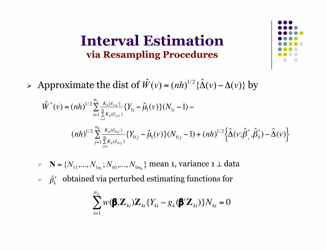
Interval Estimation via Resampling Procedures

  Approximate the dist of by

  mean 1, variance 1 ⊥ data

  obtained via perturbed estimating functions for €

ˆ W *(v) = (nh)1/ 2 Kh ( ˆ ε 1vi )

Kh ( ˆ ε 1vi )i=1

n1∑

{Y1i − ˆ µ 1(v)}(N1i −1) −i=1

n1

∑

(nh)1/ 2 Kh ( ˆ ε 0vj )

Kh ( ˆ ε 0vj )j=1

n0∑

{Y0 j − ˆ µ 1(v)}(N0 j −1)j=1

n0

∑ + (nh)1/ 2 ˆ Δ (v; ˆ β 1

*, ˆ β 0*) − ˆ Δ (v){ }

€

w(β,Z ki)Z kii=1

nk

∑ {Yki − gk (β'Z ki)}Nki = 0

Example AIDS Clinical Trial

  Objective: assess the benefit of 3-drug combination therapy vs the 2-drug alternatives across various sub-populations

  Predictors of treatment benefit:   Age, CD4wk0, logCD4wk0, log10RNAwk0

  Treatment Response:   Immune response (continuous)

  change in CD4 counts from baseline to week 24   E(Y | Z) : linear regression

  Viral response (binary)   RNA level below the limit of detection (500 copies/ml) at week 24   E(Y | Z) : logistic regression

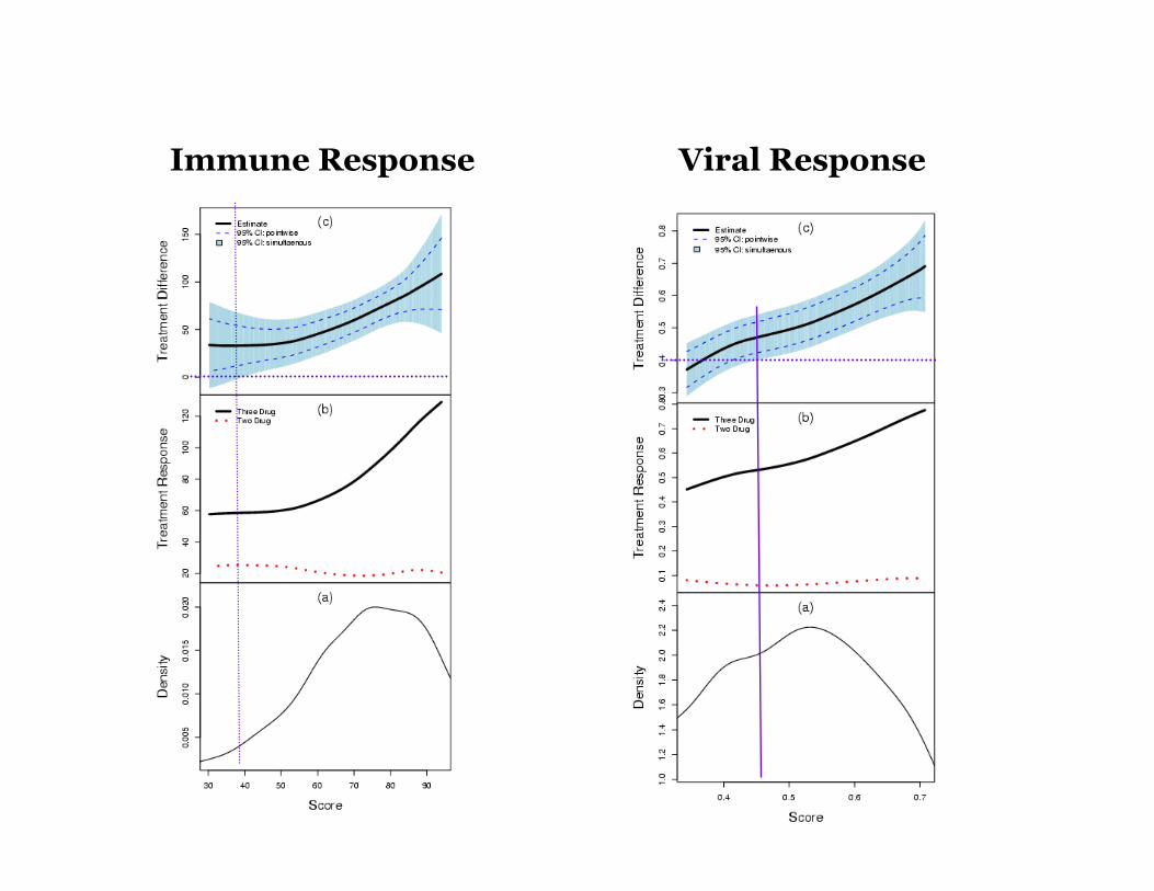
Immune Response Viral Response

Evaluating the System for Assessing Subgroup Treatment Benefits

  Cumulative residual:

  Integrated sum of squared residuals minimized under correct models

€

R(z) = E(Y1 −Y0 |Z1 = Z0 = Z) − ˆ Δ { ˆ η (Z)}[ ]Z∈Ω z∫ dF(Z)

= E{Y1I(Z1 ∈ Ωz)}− E{Y0I(Z0 ∈ Ωz)}− E[ ˆ Δ { ˆ η (Z)}I(Z ∈ Ωz)}

€

R(z)2dw(z)∫

Efficiency augmentation with auxiliary variables

  Use auxiliary variables A to obtain based on

  for example:

  Find optimal weights wopt to minimize

€

var{ ˆ Δ (v) + w' ˆ e (v)}

€

ˆ e (v) ≈ 0

€

E{ f (A1) − f (A 0) |Z1 = Z0 = Z} = 0

€

ˆ e (v) =

Kh (ˆ ε 1vi)A1ii∑

Kh (ˆ ε 1vi)i∑

−

Kh (ˆ ε 0vj )A 0 jj∑

Kh (ˆ ε 0vj )j∑

Efficiency augmentation with auxiliary variables

  Obtain optimal wopt based on the joint dist of

  Regress {Ei(v)} against {ei(v)} to obtain wopt and the augmented estimator

  The mean squared residual error of the regression, MRSE(v), while valid asymptotically, tends to under estimate the variance of the augmented estimator

€

{ ˆ Δ (v), ˆ e (v)}

€

(nh)1/ 2{ ˆ Δ (v) −Δ(v)} ≈ (nh)−1/ 2 Ei(v);i=1

n

∑ (nh)1/ 2 ˆ e (v) ≈ (nh)−1/ 2 e i(v)i=1

n

∑

€

var{ ˆ Δ w opt(v)} >> MRSE(v)

€

ˆ Δ w opt(v) = ˆ Δ (v) + wopt

' (v)ˆ e (v)

Efficiency augmentation with auxiliary variables

  To approximate the variance of

  Double bootstrap: computationally intensive   Bias correction via a single layer of resampling:

€

ˆ Δ w opt= ˆ Δ + wopt

' ˆ e

€

var( ˆ Δ w opt) ≈ MRSE + trace( ˆ Σ we

2 )

ˆ Σ we = ˆ Σ e−1 E{ˆ e *ˆ e *'ˆ ε ∗ | Data}

E{(N −1)3}ˆ ε ∗ = residual of linear regression with {( ˆ Δ b

* − ˆ Δ , ˆ e b* ),b =1,...,B}

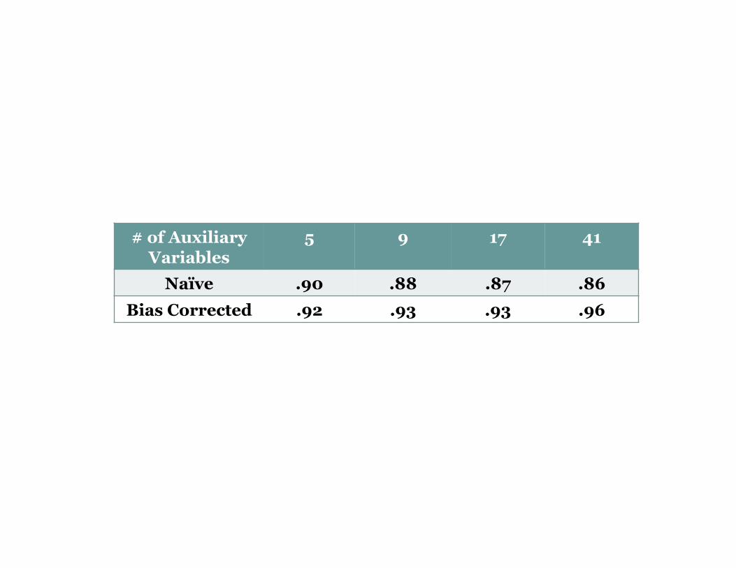
# of Auxiliary Variables

5 9 17 41

Naïve .90 .88 .87 .86 Bias Corrected .92 .93 .93 .96

Acknowledgement Joint work with Lu Tian, P. Wong and L. J. Wei

Thank you !