Embed Size (px)
Citation preview
Personality, IQ, and Lifetime Earnings
Miriam Gensowski∗
The University of Chicago
October 18, 2012
Abstract
Talented individuals are seen as drivers of long-term growth, but what makes themrealize their full potential? In this paper, I show that lifetime earnings of high-IQmen and women are substantially influenced by their personality traits, in addition tointelligence. Personality traits directly affect men’s earnings, where the effects onlydevelop fully after age 30 and increase in education. Personality and IQ also influenceearnings indirectly through education, which has sizeable positive rates of return formen in this sample. For women, born early in the 20th century, returns to educationpast a bachelor’s degree are reduced through worse marriage prospects, which offsetgains to education in terms of own earnings. The causal effect of education is identi-fied through matching on detailed background information. This paper complementsthe well-established results regarding the role of education and personality traits inexplaining life outcomes of disadvantaged children by demonstrating that they alsoaccount for considerable variation in lifetime productivity at the opposite end of theability distribution.
Key words: lifetime earnings, cognitive skills, social skills, factor analysis, human cap-ital, returns to education
JEL codes: J24, J16
∗Contact: [email protected]. I thank James J. Heckman, University of Chicago, and PeterSavelyev, Vanderbilt University, for their support in this project. Min Ju Lee and Molly Schnell haveprovided excellent research assistance in data preparation. This paper and other versions of it have benefitedfrom comments received at the Labor Working Group, University of Chicago, the Applied Economics andEconometrics Seminar, University of Mannheim, the IZA workshop on Cognitive and Noncognitive Skills,Bonn 2011, the European Association of Labor Economics, Paphos, Cyprus, September 2011, and the AEAMeetings in Chicago, January 2012. A Web Appendix with additional material and a data description canbe found at http://home.uchicago.edu/∼ mgensowski/research/Terman/TermanApp.pdf.
i

Contents
1 Introduction 1
2 The Terman Survey 22.1 IQ and Personality Measures in the Terman Sample . . . . . . . . . . . . . . 42.2 Education and Background Variables . . . . . . . . . . . . . . . . . . . . . . 7
3 The Effects of Psychological Traits on Earnings and the Rate of Return toSchooling 83.1 The Effect of Personality and IQ on Total Lifetime Earnings . . . . . . . . . 83.2 Estimation Procedure . . . . . . . . . . . . . . . . . . . . . . . . . . . . . . . 93.3 The Direct Effects of Personality Traits and IQ on Earnings . . . . . . . . . 12
3.3.1 Men . . . . . . . . . . . . . . . . . . . . . . . . . . . . . . . . . . . . 143.3.2 Women . . . . . . . . . . . . . . . . . . . . . . . . . . . . . . . . . . 20
3.4 The Effects of Psychological Traits on Educational Attainment . . . . . . . . 253.5 The Rate of Return to Schooling . . . . . . . . . . . . . . . . . . . . . . . . 29
3.5.1 The Mincer Coefficient . . . . . . . . . . . . . . . . . . . . . . . . . . 293.5.2 The IRR for Men . . . . . . . . . . . . . . . . . . . . . . . . . . . . . 303.5.3 The IRR for Women . . . . . . . . . . . . . . . . . . . . . . . . . . . 35
4 Conclusion 41
References 42
ii
1 Introduction
This paper draws on a unique sample of high-ability men and women born early in the last
century and followed over their lifetimes by the American psychologist Lewis Terman.1 The
Terman study contains rich data on the lifetime earnings, psychological traits and family
backgrounds of a cohort of high IQ men and women. These unique individuals were all
expected to excel in life, to be over-achievers and contribute to society by the sheer power of
their talent. While many of them fulfilled this expectation, their life outcomes varied greatly.
I show that a substantial amount of this variation in lifetime earnings can be explained
by personality traits, in addition to intelligence, and education. Psychological traits have
significant direct effects on earnings. These direct pricing effects do not arise until age 30 or
later. Furthermore, their magnitude is increasing in schooling — the effects are stronger for
the more highly educated men. In individual year-by-year estimates, these differences are
not statistically significant. Therefore, standard data sets, which do not contain life time
earnings data, would not identify this heterogeneity.
There are also indirect effects of personality traits and IQ on lifetime earnings, since they
alter educational attainment, and there are significant positive returns to schooling in this
sample.
I also analyze the effects of intelligence at very high levels. The data used in this paper
do so. IQ has a positive and statistically significant effect on men’s earnings, even within the
IQ range of 140–200. This effect does not only work through higher educational attainment
but also from a direct impact of ability on earnings. For women, in contrast, having a higher
IQ results in lower lifetime earnings if they were not at the top of the educational attainment
spectrum.
The cohort studied here was born in the early years of the last century when the role of
women in the labor market and society was fundamentally different than it is today (Goldin,
1The study is described in Terman and Sears (2002a); Terman et al. (2002a) and Terman and Sears(2002b); Terman et al. (2002b). It is the longest prospective cohort studies in existence, Friedman et al.(1995).
1
1992). Counting only their own earnings, the rate of return to female schooling is low
for women with less than a doctorate degree. Assortative mating leads to more profitable
matches for the more highly educated women, so education should increase their family
earnings. There is, however, an additional cost to post-graduate education for women of
this cohort: their prospects of marrying are much lower, offsetting the positive effects of
education on family earnings. Finally, women with a doctorate degree were exceptional
figures who had earnings almost as high as men.
With access to lifetime earnings histories, I can bypass the ad hoc methods widely used
to approximate the lifetime ex post rate of return from cross sections of data.2 Using full life
cycles of earnings, I present estimates of the internal rate of return to schooling and show
that it is a function of psychological traits as well. Standard application of the Mincer model
produces misleading estimates.
The paper proceeds in the following way. Section 2 discusses the rich data analyzed in
this paper. Section 3 discusses the effects of psychological traits on earnings levels and rates
of return by gender, separated into the direct and indirect effects. Section 4 concludes.
2 The Terman Survey
The analysis in this paper is based on a survey initiated by the prominent psychologist Lewis
Terman in the early 1920s to study the life outcomes of high IQ children.3 The criterion for
inclusion in the sample was having an IQ of 140 or higher.4 These high IQ school children
were identified through a procedure that canvassed all high schools in California.5 The
Terman sample consists of 856 boys and 672 girls, born around 1910. The cohort was followed
from 1922 to 1991, with surveys every 5–10 years, making it the longest prospective cohort
2See Mincer (1974) who suggests several widely used, but ad hoc, approximations.3Terman was a pioneer of IQ testing at Stanford University. He is the “Stanford” in the Stanford-Binet
IQ test.4The threshold was considered the genius level by Terman.5Part of the procedure was the Stanford-Binet test, which Terman perfected. See Terman et al. (1925)
for a description of how the sample was identified.
2
study that also has data on earnings.6 Using these, we can estimate earnings parameters
using life cycle data and not synthetic cohorts and avoid imposing the assumptions of the
Mincer model which in other research has been tested and rejected (Heckman et al., 2006).7
The Terman data is not only unusual in terms of its long follow up, but also, and possibly
even more so, in terms of its rich information about its participants Information is available
on their IQs, their personality traits, their early and current health, their background and
conditions when growing up, and other aspects of their lives, including marriage, children,
and other life events. The Terman survey samples high-ability individuals who are rarely
found in standard surveys. Given the low correlation between IQ and most personality
traits,8 we can generalize our findings on the effect of personality on earnings and other
outcomes to the wider population.
The sample used to conduct the analysis does not include the youngest and oldest partic-
ipants, since their selection into the sample was non-standard.9 Our sample consists of 766
men and 607 women who were born between 1904 and 1915. We use respondents with valid
information about their education who have observations available on all socio-emotional
trait ratings. We exclude non-Caucasian children and those with rare genetic diseases. In
order to have full earnings histories from age 18 to 75, only individuals with 10 or fewer
6Its attrition rate is less than 10%. Those who dropped out from the sample do not differ from thosewho remain in terms of income, education, and demographic factors (Sears, 1984), or psychological measures(Friedman et al., 1993a).
7The Terman data have been used extensively by psychologists but much less so by economists. Psy-chologists have focused on health and longevity outcomes. They have linked longevity to the personalitytrait of conscientiousness (Friedman, 2000, 2008; Friedman et al., 1994, 1995, 1993a; Martin et al., 2007,2002), as well as to parental divorce, durations of marriage, and number of children (Friedman et al., 1995;Martin et al., 2005; Schwartz et al., 1995; Tucker et al., 1997, 1996, 1999). The economists analyzing thisdata analyze family outcomes: Becker et al. (1977) discusses marital instability, Michael (1976) divorce, andTomes (1981) fertility and children’s schooling. The Terman retirement behavior is analyzed by Hamermesh(1984). Savelyev (2011) investigates the causal effect of higher education on longevity and the role of Con-scientiousness. Only the work by Leibowitz (1974) focuses on earnings outcomes. She estimates the effectof schooling on earnings, controlling for parental investments in their children, but the longitudinal featureof the data is ignored. Today, I have many more years of lifetime data than she does.
8See Borghans et al., 2011 for a discussion of the correlation of IQ and personality traits. Note thatOpenness to experience is an exception to the low correlation, this trait is consistently found to be positivelycorrelated to IQ.
9As described in Terman et al. (1925), most students were identified through the canvassing of schools.Few other students were included in the sample because the researchers were made aware of these intelligentchildren through other means— for example, by their siblings.
3

years of missing earnings information are retained in the sample. The sample consists of 595
men and 422 women.
I construct a full lifetime earnings history, as well as education and marriage profiles, for
each participant. 10 The earnings measures for computing the rates of return to schooling
are annual earnings after tuition, in 2010 U.S. Dollars.11 Tuition costs are estimated from
data on tuition rates at each of the colleges or universities attended by the Terman partic-
ipants. Tuition is subtracted from earnings at each year that college is attended, at both
the undergraduate and graduate level. Note that for inactive workers, who are no longer
working, as well as for the deceased, earnings are set to zero but still included in the profile.
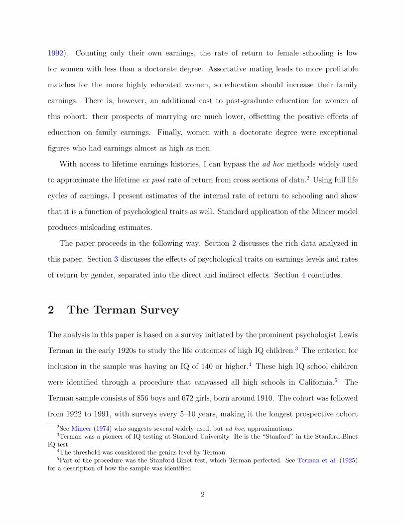
The raw earnings profiles by education are presented in Fig. 1. They follow the standard
pattern of initially higher earnings for persons who obtain less schooling, which are later
surpassed by the earnings of the more educated, once they work full-time.
2.1 IQ and Personality Measures in the Terman Sample
IQ is measured at study entry in 1922, and is the basis for inclusion in the Terman sample.12
The personality traits collected in this early survey are remarkably similar to the modern
Big Five taxonomy, even though the measures were collected some 70 years before the Big
Five were codified.13
Personality ratings are measured in 1922 and 1940. Table A-3 in the Web Appendix
10The Web Appendix A, found at http://home.uchicago.edu/∼ mgensowski/research/Terman/Terman-App.pdf, describes how the earnings profiles were constructed and specifies how tax rates or tuition costsare obtained.
11The Web Appendix C provides all of the estimates made here in this paper also on earnings after tuitionand tax, where tax rates are made a function of the marital status obtained from the Terman maritalhistories.
12Most students took the Stanford-Binet IQ test. About 30% of the students took another IQ test, theclosely related “Terman Group Test”, specifically designed for screening these high achieving children. Fora more detailed description of the tests, see Chapter I in Terman and Sears (2002a). In order to controlfor possible differences between the two measures of IQ, we allow for different regression coefficients on thedifferent measures of IQ. They are not statistically different from each other so we do not report these results.
13See Goldberg (1993). The Big Five traits are Openness, Conscientiousness, Extraversion, Agreeableness,and Neuroticism (OCEAN). While our traits are conceptually very close to the Big Five personality traits,they are not measured using the same inventory. Martin and Friedman (2000) have established that Consci-entiousness and Extraversion from the Terman questionnaires correspond closely to the analogous Big Fivetraits.
4

Figure 1: Average Earnings by Education, Minus Tuition and After Taxes
(a) Males
020
4060
8010
012
0
2010
USD
, in
th
ousa
nds
20 30 40 50 60 70
Age
Doctorate (158) Master's (113) Bachelor's (178)
Some College (102) High School (57)
(b) Females (family earnings)
020
4060
8010
012
0
2010
USD
, in
th
ousa
nds
20 30 40 50 60 70
Age
Doctorate (24) Master's (96)Bachelor's (182) High School(130)
Notes: Observation counts are given in parentheses. Earnings are average annual earnings minus tuition, in
thousand 2010 U.S. Dollars, constructed from Terman Data. For women, earnings are their own as well as
their husband’s earnings (if they are married). The tuition cost is applied in full when it occurred, i.e. we do
not assume any smoothing out of the payment streams, and we assume graduate students pay full tuition as
well. The education categories refer to the highest educational level attained in life. See the Web Appendix
http://home.uchicago.edu/~mgensowski/research/Terman/TermanApp.pdf for information on building
the earnings profiles, tuition, and the marriage history, from the raw data.
5

Table 1: Explanatory Variables Used
Control Variable Year Mean Std.dev Mean Std.dev
IQ 1922 149.4 (10.90) 148.6 (10.34)
Openness 1922 0.00 (0.85) 0.00 (0.73)
Conscientiousness 1940 0.00 (0.89) 0.00 (0.71)
Extraversion 1922 0.00 (0.70) 0.00 (0.82)
Agreeableness 1940 0.00 (0.66) 0.00 (0.57)
Neuroticism 1940 0.00 (0.59) 0.00 (0.55)
Father's highest school grade 1922 12.34 (3.61) 12.10 (3.62)
Mother's highest school grade 1922 11.57 (2.83) 11.69 (2.95)
Father's occupation: clerical or deceased 1922 26% (0.44) 24% (0.43)
Father's occupation: low-skilled 1922 16% (0.37) 15% (0.36)
At least one parent is retired or deceased 1922 3% (0.18) 4% (0.19)
Mother has occupation (not minor) 1922 11% (0.32) 10% (0.30)
Father's age when child was born 1922 33.42 (8.00) 34.17 (7.67)
Mother's age when child was born 1922 28.64 (5.39) 29.54 (5.36)
Either parent is born in Europe 1922 13% (0.34) 12% (0.32)
Childhood family finances (very) limited 1950 38% (0.49) 38% (0.49)
Childhood family finances abundant 1950 4% (0.20) 6% (0.23)
Childhood parental social status - high 1950 35% (0.48) 33% (0.47)
Number of siblings 1940 1.8 (1.60) 1.8 (1.62)
Birth order 1940 1.8 (1.27) 2.0 (1.39)
No breastfeeding 1922 9% (0.29) 9% (0.29)
Birthweight in kilograms 1922 3.8 (0.65) 3.6 (0.63)
Sleep is sound 1922 97% (0.17) 98% (0.14)
Cohort: 1904-1910 56% (0.50) 53% (0.50)
Cohort: 1911-1915 44% (0.50) 47% (0.50)
WWII combat experience 1945 10% (0.30) 0% (0.07)
FemalesMales
Ear
ly
Hea
lth
C
ohor
t In
foP
sych
. Tra
its
Par
enta
l Bac
kgro
un
dSi
b-
lings
6
presents the items used to measure each trait. Two personality traits are measured in
1922: Openness and Extraversion. Extraversion is indicated by the subject’s “fondness for
large groups,” “leadership,” and “popularity with other children” as rated by teachers and
parents (where we take the average of both ratings). Openness is extracted from ratings of
the subject’s “desire to know,” “originality,” and “intelligence.”14
The other three traits are based on self-ratings in 1940: Conscientiousness, Agreeableness,
and Neuroticism. The dedicated items for each are either from the personality inventory,15
where questions about usual behavior and feelings can be answered “yes,” “no,” and “?,” or
self-ratings of personality traits on an 11-point scale. Examples of Conscientiousness items
are self-ratings of “persistence” or “In your work do you usually drive yourself steadily?”
Neuroticism is based on measurements on “moodiness” or “Are your feelings easily hurt?”
etc. Agreeableness items are, for example, “easy to get along with,” or “Are you always
careful to avoid saying anything that might hurt anyone’s feelings?”.
2.2 Education and Background Variables
We have detailed information on the educational status and attainment of the Terman par-
ticipants. We also have information on father’s and mother’s backgrounds (education, occu-
pation, social status, region of origin, age at birth of subject), family environment (family’s
finances when growing up, number of siblings, birth order), and early childhood health
(birthweight, breastfeeding, sleep quality in 1922).
Descriptive statistics of the covariates that will be used as control variables are listed
in Table 1. Further descriptive statistics of variables used in this paper are presented in
Appendix Tables A-1 and A-2.
14Since “intelligence” is a facet of Openness, it might seem as if Openness and IQ measure the sameunderlying trait (see the discussion in Almlund et al., 2011). Note that the IQ test is a direct measureof the subject’s cognitive ability, while the parents’ and teachers’ ratings describe their impressions of thechild. Furthermore, several measurements of these impressions combine to generate the factor defined bypsychologists as “Openness.” Hogan and Hogan (2007) define the Big Five Openness as the degree towhich a person needs intellectual stimulation, change, and variety. Openness is correlated with IQ (r = .16,significantly different from zero). Other personality traits have much lower correlations with IQ.
15The Bernreuter scale (see Terman et al., 2002a).
7
3 The Effects of Psychological Traits on Earnings and
the Rate of Return to Schooling
IQ and personality traits, at least some of them, influence lifetime earnings of men and women
in the Terman sample. The association between the sum of discounted lifetime earnings and
these traits is discussed in Section 3.1. But observing that psychological traits are associated
with total earnings does not tell us where, or when these traits might influence earnings.
One can think of at least two channels: (1) a direct influence on wages in the marketplace,
i.e. through a direct pricing of the traits; and (2) an indirect channel through educational
attainment. The pricing of traits might occur early or late in a person’s working life. Also,
the price might be a function of the person’s educational attainment. If psychological traits
such as IQ alter the probability of obtaining higher education, and if there is a positive
return to education, the traits alter a person’s lifetime earnings potential indirectly.
After presenting the total effects of IQ and personality traits on the life-time earnings
of the Terman men and women (Section 3.1), and discussing the estimation procedures
Section 3.2 , the two channels are examined. Section 3.3 analyzes the direct effect, or the
prices of traits, by education level, for men and women. Section 3.4 shows the indirect effect
by asking how educational sorting is a function of psychological traits. The rate of return to
education, which determines the magnitude of the indirect effect, is examined in Section 3.5
3.1 The Effect of Personality and IQ on Total Lifetime Earnings
The total effects of personality and IQ on lifetime earnings16 of men and women in the
Terman sample are shown in Table 2. Personality traits and IQ clearly play a large role in
determining lifetime earnings of males. Ceteris paribus, lifetime earnings are higher if the
men are more conscientious and extraverted, and if they are less agreeable. Earnings are
16Lifetime earnings are the sum of each individual’s earnings from age 18 to age 75; for women, wealso consider the sum of their husbands’ earnings and the resulting family earnings. Family earnings forthe males can not be evaluated because the men in the sample were never asked to report their spouse’searnings, whereas the females were regularly asked about their husband’s income.
8
also increasing in IQ. It is remarkable that even in this sample, where IQs are restricted to
the top range, IQ is still positively and significantly associated with lifetime earnings. An
increase of IQ by 15 points would increase discounted lifetime earnings by 210 thousand
dollars, controlling for education and background variables. This contradicts the claim by
Gladwell (2008) that for the Terman men, IQ does not matter once family background and
other observable personal characteristics are taken into account. Even at the high end of the
ability distribution, additional IQ has meaningful consequences.
Women’s own earnings (column (2)) are also significantly increased by Conscientiousness;
but for them lifetime earnings are not higher if they are more extraverted. Instead, they are
higher for women who score higher on Openness to experience, and lower on Neuroticism.
More extraverted women have higher lifetime earnings from their spouse (column (3)). Since
for Neuroticism and Openness to experience, the lifetime effects on own and spouse’s earnings
have opposite signs, women’s family earnings (column (4)) are in fact only a significant
function of Conscientiousness and Extraversion. Generally, the effects of personality traits
on life-time earnings are much smaller for women.
3.2 Estimation Procedure
All effects of education and personality traits on earnings are identified using the rich set of
background and psychological variables at our disposal, in order to correct for any selection
problems into educational status. Thus “selection on observables” (Heckman and Robb,
1985) or a “matching” assumption are invoked. The specific implementation based on this
assumption is Ordinary Least Squares.17
We estimate the following linear specification for earnings at age t, for persons with
17The results are not a function of the linearity — other models, including a nonparametric one, yield thesame effects of education and personality traits. The description of these, and a comparison of the results,is in the Web Appendix Section C.8.
9
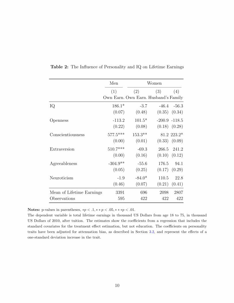
Table 2: The Influence of Personality and IQ on Lifetime Earnings
Men Women
(1) (2) (3) (4)
Own Earn. Own Earn. Husband’s Family
IQ 186.1* -3.7 -46.4 -56.3
(0.07) (0.48) (0.35) (0.34)
Openness -113.2 101.5* -200.9 -118.5
(0.22) (0.08) (0.18) (0.28)
Conscientiousness 577.5*** 153.3** 81.2 223.2*
(0.00) (0.01) (0.33) (0.09)
Extraversion 510.7*** -69.3 266.5 241.2
(0.00) (0.16) (0.10) (0.12)
Agreeableness -304.9** -55.6 176.5 94.1
(0.05) (0.25) (0.17) (0.29)
Neuroticism -1.9 -84.0* 110.5 22.8
(0.46) (0.07) (0.21) (0.41)
Mean of Lifetime Earnings 3391 696 2098 2807
Observations 595 422 422 422
Notes: p-values in parentheses, ∗p < .1, ∗ ∗ p < .05, ∗ ∗ ∗p < .01.
The dependent variable is total lifetime earnings in thousand US Dollars from age 18 to 75, in thousand
US Dollars of 2010, after tuition. The estimates show the coefficients from a regression that includes the
standard covariates for the treatment effect estimation, but not education. The coefficients on personality
traits have been adjusted for attenuation bias, as described in Section 3.2, and represent the effects of a
one-standard deviation increase in the trait.
10

schooling level j, Yj,t:
Yj,t = Xtβt + θδj,t +Dj,tνt,j + ρt,j, t = 1, . . . , T ; j = 1, . . . , J, (1)
where Xt is a vector of background variables, θ is a vector of traits (IQ and personality
factors), Dj,t is a dummy variable that equals 1 if a person is at schooling level j (of J
possible schooling levels) at age t, defined in a mutually exclusive fashion (so∑J
j=1Dj,t = 1
for all t) and νt,j is the average effect of schooling. Equation (1) is estimated separately for
men and women. In fact, as the results will show, the null hypothesis that δj,t = δj for all
t can not always be rejected at common significance levels for the t individually. Therefore,
the δj,t are subsequently also estimated as constant across education levels. The exact link
to the standard Roy model of counterfactuals is presented in Web Appendix B.
The psychological traits are summarized by factor scores, which are estimated using
the Bartlett method, based on a standard linear factor model 18. Since the estimation
of factor scores introduces error, the naive least squares estimates suffer from attenuation
bias. They can be corrected for estimation error using the method of Croon (2002).19 All
standard errors are bootstrapped accounting for the fact that the predictions are based
on an estimation of the measurement system.20 In all estimations, unless otherwise noted,
condition on personality traits (using extracted factors), IQ and family background variables
discussed in the preceding section.
Note that we allow explicitly for the effect of personality traits and IQ, δj,t, to vary
by educational level. This means that the treatment effect of education is allowed to be
heterogeneous, or in other words that there is an interaction between the education and
18See Bartlett (1937); Thomson (1938). The often-used regression method based on Thurstone (1935)results in estimates of the factor scores which are biased with respect to their means, and more importantlyfor the error correction method we are interested in, their covariance structure.
19For applications of Croon’s method, see Heckman, Malofeeva, Pinto, and Savelyev (2011) and Heckman,Schennach, and Williams (2011).
20It is standard practice to bootstrap the standard errors or estimate them with other Monte Carlomethods (Bolck et al., 2004). Even though Hoshino and Shigemasu (2008) have presented a formula thateliminates the need for simulations, their proposed solution is only valid in applications with large numbersof observations and measurements.
11

traits in their effect on earnings. As the next section will show, this is an important aspect
for the Terman men.
3.3 The Direct Effects of Personality Traits and IQ on Earnings
Now consider the first channel of influence of psychological traits on lifetime earnings —
the direct effect they have on earnings, holding constant educational attainment. How are
psychological traits priced in the marketplace? When do gains or losses occur? And is the
pricing of traits independent of the educational attainment?
We find that some traits are highly rewarded in the marketplace, and that the largest
effects (both positive and negative) arise later in the working life. And the lifetime effects of
personality traits are indeed a function of educational attainment, thus altering the payoff
from education depending on a persons personality profile.
An overview is provided by Table 3, which shows the direct effects on total lifetime
earnings. For this table, Eq. (1) was estimated on Y Ti =
∑75t=18 Yit. The different levels of
education, j, are “Bachelor’s or less” and “Master’s or more.”
For men, as in the total effect, the direct effect of IQ is positive and statistically signifi-
cantly different from zero. Therefore, the lifetime effect of IQ on earnings is not only driven
by higher educational attainment associated with higher IQ, but also through a direct impact
on earnings. IQ impacts earnings similarly across education levels. Conscientiousness, and
Extraversion, are associated with higher earnings regardless of education level. The reward
to being more conscientious and extraverted, however, is greater for more highly educated
men. This difference is statistically significant with p-values of 6% and 1%, respectively.
More agreeable men earn less, especially so if they are in the highly educated category of
having a Master’s or a doctorate degree. Interestingly, more neurotic men seem to earn more
when they are in this education category. While the point estimate is not significant, the
difference to the point estimate for less educated men is significant.
Women’s IQ is strongly negatively related to lifetime earnings for women with at most
12
a Bachelor’s degree, but not for the most highly educated women. The difference is highly
significant too. Women of this highly select sample who obtained at most a Bachelor’s degree
have lower earnings husbands when their IQs are in the highest ranges as opposed to “just
above 140.” This surprising negative effect, however, is limited to women who did not achieve
the highest educational attainments. Apparently, women with a Master’s or more are able
to avoid this wage penalty to higher IQs. Women with high scores in Openness to experience
benefit from this trait, either in terms of own earnings (Master’s or more) or family earnings
(Bachelor’s or less), whereas it is insignificant for men. As for men, Conscientiousness has
a positive effect on earnings, but only so for women with at most a Bachelor’s degree. The
effect on the more highly educated women is inconclusive. So are the effects of Extraversion
and Agreeableness. Surprisingly, women with less education seem to have higher lifetime
earnings if they score higher on Neuroticism.
The bottom half of Table 3 highlights the importance of accounting for heterogeneous
effects of the personality traits by educational attainment. For men, Conscientiousness,
Extraversion, and Neuroticism have statistically significantly different effects on lifetime
earnings. For women, education matters for the effects of IQ, Openness, Conscientiousness,
and Extraversion. Standard analyses without interactions ignore this heterogeneity and over-
or under-state the effects of these traits when considering the average impacts only.
13

3.3.1 Men
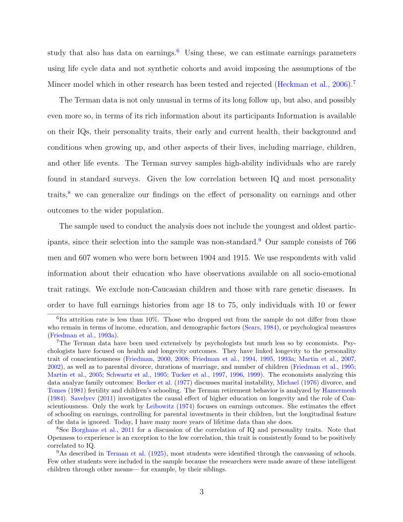
Figure 2 (page 18) presents the effects of personality traits and IQ on lifetime earnings of
the Terman males, by education. This means the δj,t are plotted over time t for two j,
either “Bachelor’s degree or less,” or “Master’s or doctoral degree.” While the effects vary
by education, the graphs reveal that the direct effects, when estimated age-by-age, are not
statistically significantly different from each other.21
Since the signs of the effects are equal across the education levels, except for Neuroticism,
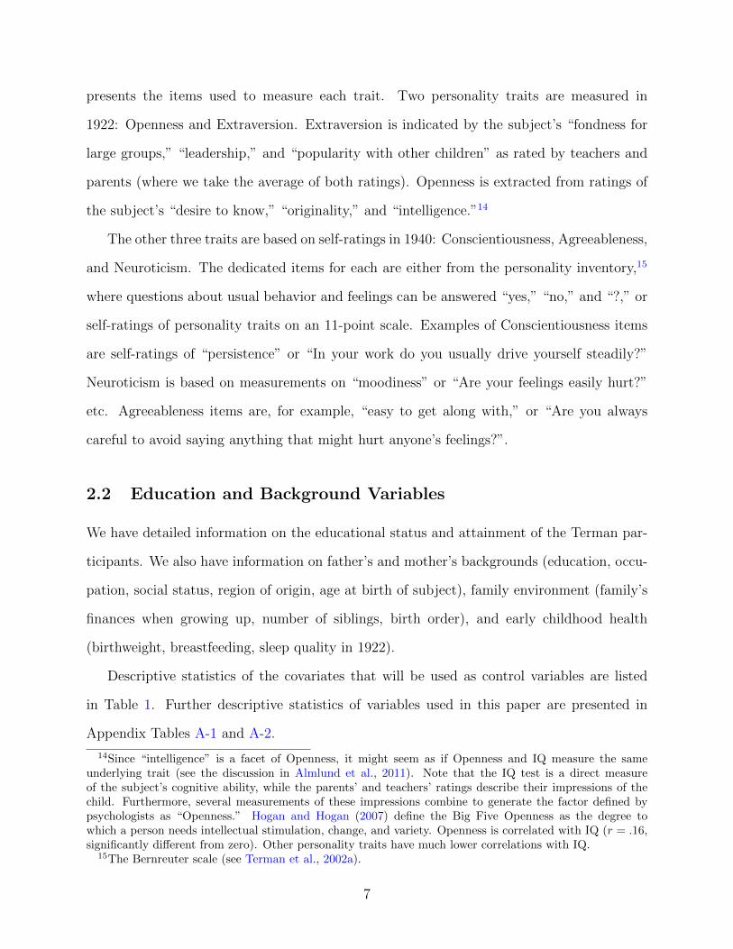
a sparser model that does not estimate the δj,t by education level is a good benchmark. In
the common coefficient model, all δj,t are forced to δj,t = δj:
Yj,t = Xtβt + θδt +Dj,tνt,j + ρt,j, t = 1, . . . , T ; j = 1, . . . , J, (2)
Figure 3 shows the results of estimates according to this common coefficient model, where
indeed the standard errors are tighter.
IQ, even in this selective group, is still associated with higher earnings. This means that
the lifetime effect of IQ is at least partly caused by a direct effect on earnings. Conscien-
tiousness is also strongly positively associated with earnings. For both IQ and Conscien-
tiousness, the effects are always positive, but they are largest during the prime working years
- from 40 to 60. One explanation for the strong effects which are absent from the early years
could be related to work effort: Since the measure of earnings provided by the Terman data
are only annual earnings, not hourly wages, it could very well be that more conscientious
individuals work longer, and longer hours. This would link back to the literature on the
role Conscientiousness plays in health (Lodi-Smith et al., 2010). It has been shown that
more conscientious individuals live longer (Friedman et al., 1993b; Weiss and Costa, 2005).
They are less likely to experience the chronic illnesses which are main predictors of mortality
(Goodwin and Friedman, 2006; Marks and Lutgendorf, 1999; Mokdad et al., 2004), at least
21The Appendix shows the difference between the coefficients and the associated 95% confidence bands ofthe difference, which include zero.
14
partly because they display better health-related behaviors, such as better prevention and
fewer activities that endanger health (Roberts et al., 2005). Men who score highly on Ex-
traversion have significantly higher earnings. Comparing two otherwise equal men where
one scores one standard deviation higher on Extraversion, he will earn up to 20,000 USD
(2010) per year more than his less outgoing counterpart.
Agreeableness in the common coefficient model is not precisely estimated - the lifetime
earnings effect are more negative (and only significant) for more highly educated men. By
combining coefficient, this impact is lost. Muller and Plug (2004) find that antagonistic (or
less agreeable) men earn more - in this sense, the Terman findings are similar.22 Openness
never seems to have a positive effect on earnings, but it is not statistically precisely estimated,
and even the effect on total lifetime earnings is not statistically significantly different from
zero. Because of its positive correlation with IQ, Openness is often found to have a positive
effect on earnings in analyses that do not control for IQ. These results are upwardly biased.
The Terman study is a case study of a group of persons with similar IQs that also provides
a direct IQ score. Controlling for IQ, Openness does not have a clear effect on earnings.
Finally, we can conclude that Neuroticism does not affect earnings in the Terman sample.
The effects of personality traits on earnings are very small in the early years of the
working life, until about age 30. Therefore, having access to data that combines measures of
personality traits and IQ with long follow-up is essential. One can only describe the effects
of these traits in a satisfying manner with earnings measures that extend well into the prime
working years. The effects of Conscientiousness, Extraversion, and IQ only materialize after
the thirties. Researchers who only have access to earnings observations for the early working
life would likely find that these personality traits have no significant association, or very
small ones, with earnings. 23
22Interestingly, these authors show that Conscientiousness is not statistically significantly different fromzero for men in the Wisconsin Longitudinal Study; whereas the measure in Terman is clearly significant.
23A caveat about causality is in order. In contrast to the estimated effect of education on earnings, whichwe can interpret as causal under the assumptions of this paper, the estimated effect of personality should beinterpreted with caution. Researchers have debated whether reverse causality is a serious threat to validity inthe analysis of the effect of personality on earnings. They are concerned with the possibility that personality
15

traits in mid-life are actually the result of previous labor market experience. Then, the association of acertain trait with earnings is not necessarily causal. Most researchers use early measures of personality, sothat these pre-date the outcome measures. This timing of measurements makes the interpretation of traitscausing outcomes more credible. Yet, early traits are not hypothesized to cause outcomes, but concurrenttraits. Thus, this method comes at the cost of not using the measure of personality that drives observedearnings (see Almlund et al., 2011).We follow the approach of using early measures of IQ, Openness and Extraversion. However, the otherpersonality traits are measured in 1940 — when the Terman participants are aged 25–35. While claims ofcausality have to be guarded, we do think the results are showing earnings gains due to personality and IQfor two reasons. First, we perform a robustness analysis to test whether the 1940 measures of personalitytraits are a function of early labor market success. We extract the personality factors conditionally on wagesprior to 1940, wages at age 25, education, and age, and estimated the effects of these factors on wages (in theWeb Appendix C, Section C.7). The estimated effect is not altered much by this conditioning. Second, notethat the strongest associations of the personality traits with earnings arise later in the working life. Underreverse causality, one would expect them to be strongest early on since the early labor market success (i.e.high wages) would cause the personality trait. Since the opposite is observed, even for the traits measuredin 1940, the argument that our results are driven by reverse causality is weaker.
16
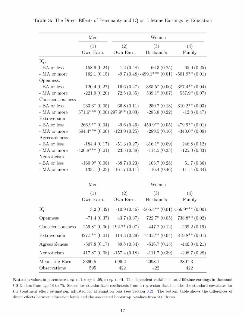
Table 3: The Direct Effects of Personality and IQ on Lifetime Earnings by Education
Men Women
(1) (2) (3) (4)
Own Earn. Own Earn. Husband’s Family
IQ:
- BA or less 158.9 (0.24) 1.2 (0.48) 66.3 (0.25) 65.0 (0.25)
- MA or more 162.1 (0.15) -9.7 (0.48) -499.1*** (0.01) -501.9** (0.01)
Openness:
- BA or less -120.4 (0.27) 16.6 (0.47) -385.5* (0.06) -387.4** (0.04)
- MA or more -221.9 (0.20) 72.5 (0.35) 539.1* (0.07) 557.9* (0.07)
Conscientiousness
- BA or less 233.3* (0.05) 66.8 (0.11) 250.7 (0.13) 310.2** (0.03)
- MA or more 571.6*** (0.00) 297.9** (0.03) -285.8 (0.22) -12.8 (0.47)
Extraversion
- BA or less 266.9** (0.04) -9.6 (0.46) 450.9** (0.05) 479.9** (0.01)
- MA or more 694.4*** (0.00) -123.9 (0.25) -289.5 (0.16) -340.0* (0.09)
Agreeableness
- BA or less -184.4 (0.17) -51.3 (0.27) 316.1* (0.09) 246.8 (0.12)
- MA or more -420.8*** (0.01) 23.5 (0.38) -114.5 (0.33) -125.0 (0.33)
Neuroticism
- BA or less -160.9* (0.08) -38.7 (0.23) 103.7 (0.28) 51.7 (0.36)
- MA or more 133.1 (0.23) -161.7 (0.11) 16.4 (0.46) -111.4 (0.34)
Men Women
(1) (2) (3) (4)
Own Earn. Own Earn. Husband’s Family
IQ 3.2 (0.42) -10.9 (0.46) -565.4** (0.01) -566.9*** (0.00)
Openness -71.4 (0.37) 43.7 (0.37) 722.7* (0.05) 738.8** (0.02)
Conscientiousness 259.8* (0.06) 192.7* (0.07) -447.2 (0.12) -269.2 (0.19)
Extraversion 427.5** (0.01) -114.3 (0.29) -740.3** (0.04) -819.8** (0.01)
Agreeableness -307.8 (0.17) 89.8 (0.34) -516.7 (0.15) -446.0 (0.21)
Neuroticism 417.8* (0.08) -157.4 (0.18) -111.7 (0.39) -208.7 (0.28)
Mean Life Earn. 3390.5 696.2 2098.1 2807.3
Observations 595 422 422 422
Notes: p-values in parentheses, ∗p < .1, ∗ ∗ p < .05, ∗ ∗ ∗p < .01. The dependent variable is total lifetime earnings in thousand
US Dollars from age 18 to 75. Shown are standardized coefficients from a regression that includes the standard covariates for
the treatment effect estimation, adjusted for attenuation bias (see Section 3.2). The bottom table shows the differences of
direct effects between education levels and the associated bootstrap p-values from 200 draws.
17
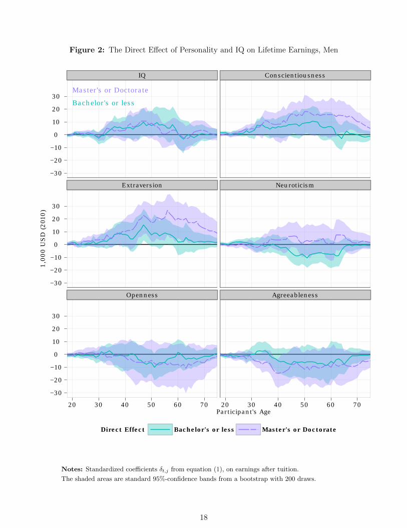
Figure 2: The Direct Effect of Personality and IQ on Lifetime Earnings, Men
Bachelor's or less
Master's or Doctorate
IQ Conscientiousness
Extraversion Neuroticism
Openness Agreeableness
−30
−20
−10
0
10
20
30
−30
−20
−10
0
10
20
30
−30
−20
−10
0
10
20
30
20 30 40 50 60 70 20 30 40 50 60 70Participant's Age
1,0
00 U
SD
(201
0)
Direct Effect Bachelor's or less Master's or Doctorate
Notes: Standardized coefficients δt,j from equation (1), on earnings after tuition.
The shaded areas are standard 95%-confidence bands from a bootstrap with 200 draws.
18

Figure 3: The Direct Effect of Personality and IQ on Lifetime Earnings, Men, Common Coefficient
IQ Conscientiousness
Extraversion Neuroticism
Openness Agreeableness
−20
−10
0
10
20
30
−20
−10
0
10
20
30
−20
−10
0
10
20
30
20 30 40 50 60 70 20 30 40 50 60 70Participant's Age
1,0
00 U
SD
(201
0)
Notes: Standardized coefficients δt from equation (2), on earnings after tuition.
The shaded areas are standard 95%-confidence bands from a bootstrap with 200 draws.
19
3.3.2 Women
For women, the estimates of the effects of personality traits and IQ on earnings are generally
more noisy than for men. There are at least three reasons for this: For women, we are
analyzing family earnings, which are constituted of the husband’s earnings, and own earnings.
The same trait may have different effects on these two types of earnings. Secondly, there
are fewer women than men in the Terman sample, so for the same number of covariates
the estimates are less precisely determined. Thirdly, in the case of women, the few with a
doctorate degree are so particular, and have very different earnings streams, that they can
almost be considered outliers.
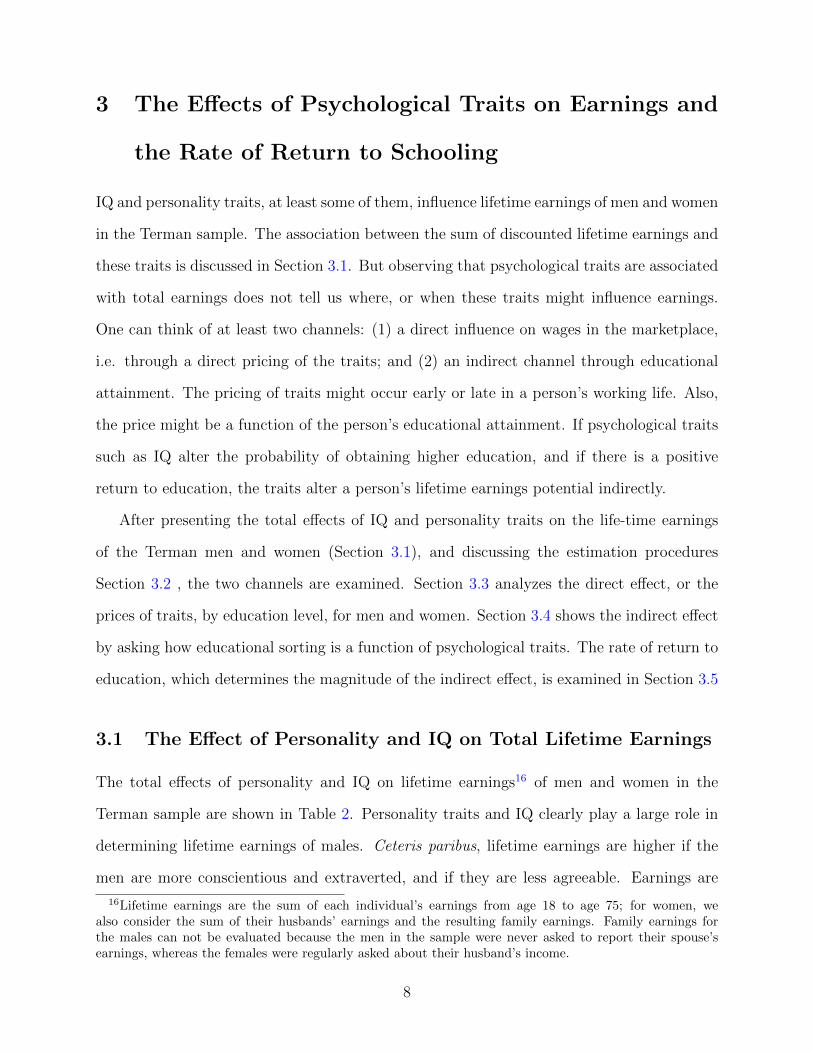
Figure 4 shows the direct effects of personality traits on the combined earnings of Terman
females and their husbands.24 The most striking feature of the effects are how large the
confidence bands are for women with a doctorate or Master’s degree (in purple), whereas
they are more reasonable for the less educated women.25 Only 28% of women in our sample
are in this high education category, or 120 women, leading to the noisy estimates. When
looking at the differences between effects by education level, they clearly exist in levels,
but the confidence bands overlap largely. Remember, however, that the differences are
statistically significant for lifetime earnings in IQ, Openness, and Extraversion.
While it is clear that since the effects are so noisy that one should not be confident about
their size or sign, knowing their constituents is of interest. In particular, since we know that
the direct effect of Extraversion on lifetime earnings, for example, are significantly different
between women with a Master’s degree or higher as opposed to women with a Bachelor’s
degree or less, it is important to see whether the difference is driven by the same components
having different effects, or by different components. Figures 5 and 6 show, in blue or pink
color, the stacked effects of traits on the husband’s or own earnings, that together make up
24The full set of figures also for own and husband’s earnings separately can be found in the Web AppendixC.
25Note that in the case of women, the common coefficient model 2 does not yield estimates of the directeffects that are statistically significantly different from zero age-by-age, as was the case for men in Fig. 3,even if we exclude the women with a doctorate degree from the estimation.
20

family earnings. And indeed, the overall positive effect of extraversion for women with a
Bachelor’s or less is almost entirely driven by the effect of extraversion on husbands’ earnings.
More extraverted women marry more frequently, or more higher earning husbands. In the
case of women with a Master’s degree or more, highly extraverted women have men who
are earning slightly less, and they also tend to earn less themselves. Individually, these
two effects are not statistically significantly different from zero, but taken together they are
significantly different over a lifetime (Table 3), as is the positive effect of extraversion for the
less highly educated women.
Openness is the mirror image of Extraversion; highly educated women benefit from hav-
ing intellectual taste and being open to new experiences, whereas women with at most a
Bachelor’s have lower earnings when they score higher on this trait.
In general, the pink slices representing the effects of personality and IQ on women’s
own earnings are very small. A likely explanation for the lack of association between own
earnings and the Terman females’ traits is that fertility and the probability of marriage are
not significantly associated with personality traits within this sample.26 Since much of the
labor market behavior can be attributed to their family status, it is not surprising to find
that traits and IQ do not influence the women’s earnings in a meaningful way. The lack of
effects is not only driven by zero earnings of many housewives: when I estimate these effects
only on a subsample of women who have earnings of ten thousand dollars per year or more
for at least 20 out of the 48 working years between age 18 and 65, the effects are still very
small and not statistically significantly different from zero.
Figures Figs. 5 and 6 demonstrate how educational attainment alters the effect certain
personality traits have on the earnings they receive through their husbands - IQ, Extraver-
sion, and Openness affect their potential in the marriage market differently depending on
whether they have a Bachelor’s or less, or a Master’s or doctorate degree.
26Tables not shown but available upon request.
21

Figure 4: The Direct Effect of Personality and IQ on Lifetime Earnings, Women
IQ Conscientiousness
Extraversion Neuroticism
Openness Agreeableness
−20
0
20
40
−20
0
20
40
−20
0
20
40
20 30 40 50 60 70 20 30 40 50 60 70Participant's Age
1,0
00 U
SD
(201
0)
Direct Effect Bachelor's or less Master's or Doctorate
Notes: Standardized coefficients δt,j from equation (1), on family earnings after tuition.
The shaded areas are standard 95%-confidence bands from a bootstrap with 200 draws.
22

Figure 5: The Direct Effect of Personality and IQ on Lifetime Earnings,Women with a Bachelor’s degree or less
IQ Conscientiousness
Extraversion Neuroticism
Openness Agreeableness
−20
0
20
−20
0
20
−20
0
20
20 30 40 50 60 70 20 30 40 50 60 70Participant's Age
Trea
tmen
t E
ffec
t, in
1,0
00 U
SD
(201
0)
Treatment Effect Family Earnings w 95% Conf.Int.
Husband's Earn. Own Earn.
Notes: Standardized coefficients δj,t from equation (1), for j = Bachelor’s degree or less, on three earnings
types: women’s own earnings (pink shade), their husband’s earnings (blue shade) and the combined family earnings after
tuition (black solid line, with a 95% confidence band, shaded gray).
23
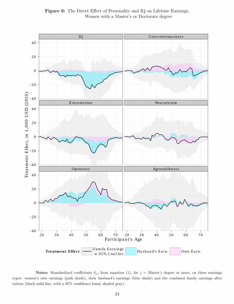
Figure 6: The Direct Effect of Personality and IQ on Lifetime Earnings,Women with a Master’s or Doctorate degree
IQ Conscientiousness
Extraversion Neuroticism
Openness Agreeableness
−40
−20
0
20
40
−40
−20
0
20
40
−40
−20
0
20
40
20 30 40 50 60 70 20 30 40 50 60 70Participant's Age
Trea
tmen
t E
ffec
t, in
1,0
00 U
SD
(201
0)
Treatment Effect Family Earnings w 95% Conf.Int.
Husband's Earn. Own Earn.
Notes: Standardized coefficients δj,t from equation (1), for j = Master’s degree or more, on three earnings
types: women’s own earnings (pink shade), their husband’s earnings (blue shade) and the combined family earnings after
tuition (black solid line, with a 95% confidence band, shaded gray).
24

3.4 The Effects of Psychological Traits on Educational Attainment
An emerging literature shows that psychological traits can be linked to educational attain-
ment. A summary is provided by Almlund et al. (2011), who report on findings from repre-
sentative datasets in the U.S., The Netherlands, and Germany. Conscientiousness is consis-
tently found to have a strong association with years of education, and its effect (correlation)
is the strongest among the psychological traits and exceeds that of IQ. More conscientious
individuals stay in school longer. Extraversion, Agreeableness, and Neuroticism have weaker
associations with education. Openness exhibits a positive association, but is known to be
moderately correlated with IQ. Hence this finding could reflect the role of IQ, rather than
an own independent relation to schooling, as IQ is not controlled for in these studies.
Based on a generalized ordered logit model of education choice,27 presented in Table 4, I
find that psychological traits play roles that are similar to those found in the literature, but
that the effects differ substantially by level of education, and slightly by gender.
Conscientiousness is generally associated with higher schooling attainment for both
men and women in this sample, even controlling for all background factors and other psy-
chological traits. For males, Conscientiousness positively affects the probability of passing
the thresholds of Bachelor’s degree, Master’s degree, and Doctorate (see Table 4). For fe-
males, it significantly increases the chance of obtaining a master’s degree or higher. Thus,
at each of these thresholds, more conscientious men and women are less likely to remain
in any of the education levels that are lower, in comparison to the threshold or a higher
education level. Conscientiousness likely enhances education through lowering the psychic
27The generalized ordered logit model (e.g., Williams, 2006) is a collection of binary logit models for eachof N − 1 thresholds of N ordered choices. In this paper, the four thresholds are the following: (1) somecollege, (2) Bachelor’s, (3) Master’s, and (4) Doctorate. For instance, a binary logit model for the threshold“Bachelor’s” estimates the choice of Bachelor’s degree or above vs. some college education or high schooldiploma. The generalized ordered logit model is equivalent to the ordered logit model when the coefficientsfor each regressor are restricted to be the same for all binary logits within the generalized model. Equalityof these coefficients is called the parallel regression assumption, which we test and reject for the Termandata. Thus, the more parsimonious ordered logit model should not be used. Another alternative model, themultinomial logit, relies on the independence of irrelevant alternatives assumption, which is not supportedby the Terman data.
25
costs of education, lowering the discount rate, and helping to imagine the future better. The
“hard working” element of Conscientiousness implies that a conscientious person perceives
the effort needed to achieve a higher educational attainment as less costly. The “future
planning” element of Conscientiousness can be thought of as being associated with lower
discount rates for deferred gains. Finally, a greater propensity to plan for the future could
decrease the effort needed to imagine future outcomes and to correctly evaluate the costs
and gains involved in the long-term investments of obtaining higher education.
Openness is also significantly associated with higher education levels in the Terman
sample. Men with a higher Openness score are more likely to obtain a bachelor’s degree
or more, and women are more likely to achieve a master’s or doctorate degree. This result
helps to resolve the uncertainty in the literature about the role of Openness in predicting
educational attainment. Openness positively affects education even conditioning on IQ.
Apart from Conscientiousness and Openness, the effects of other psychological traits differ
by gender. This might reflect the different role that education played for the females of this
cohort compared to the role of education for males. IQ significantly increases the chances of
obtaining a Bachelor’s degree or more for Terman men. Somewhat counterintuitively, women
with a higher IQ are less likely to pass the threshold of a doctorate degree than Terman
women with a lower IQ. Yet, the result is less puzzling when we remember two facts: All
Terman women had an exceptionally high IQ, so we are not comparing low-IQ women to
high-IQ women. Also, the threshold in question is very high and only few women of this
cohort obtained a doctorate degree (6%). This low percentage is in line with the evidence
that this was an unusual and difficult path in the first half of the Twentieth century.28
The associations between education and Extraversion, Agreeableness, and Neuroticism
for Terman females are similar to findings in previous studies, where representative samples
of men and women were used. The associations for Terman males diverge from these pooled
samples.
28The share of Terman males who obtained a Doctorate is 27%.
26
The effect of Extraversion on educational choice is negative for females. One expects
this negative effect (socializing takes time away from studies), and it has indeed been found
in previous studies for representative samples of men and women. More extraverted Terman
women are less likely to pass the thresholds of a bachelor’s degree as well as a doctorate
degree. For Terman men, extraversion has no significant effect on educational attainment,
which is not what other researchers find.
Finally, Agreeableness and Neuroticism29 negatively affect the choice of education
above high school for females, which is in line with previous results on the effects of Agree-
ableness and Neuroticism on the educational choices of men and women in the general
population (Almlund et al., 2011; Baron and Cobb-Clark, 2010). Neuroticism increases the
likelihood of choosing at least a bachelor’s degree for men.
Thus, traits influence education, but their effects depend on gender as well as the ed-
ucational margin considered. The educational sorting of Terman females by psychological
traits is similar to what other researchers have found based on representative datasets, where
men and women were pooled together. It would be interesting to contrast our findings on
Extraversion, Agreeableness, and Neuroticism to results from representative datasets where
the associations are broken out by gender as well. Conscientiousness and Openness have a
similar role in the Terman sample for both men and women: they increase the probability
of choosing higher educational levels. This is in line with previous results. Furthermore, we
can establish that Openness has a positive role in enhancing education that is independent
of IQ.
29The reverse of Neuroticism is Emotional Stability, and in this text we denote with these the two endpoints of the scale. This differs from the practice in the current psychological literature, where Neuroticismis sometimes reverse-coded so that by high Neuroticism the researchers actually denote high EmotionalStability, or “positive Neuroticism.”
27
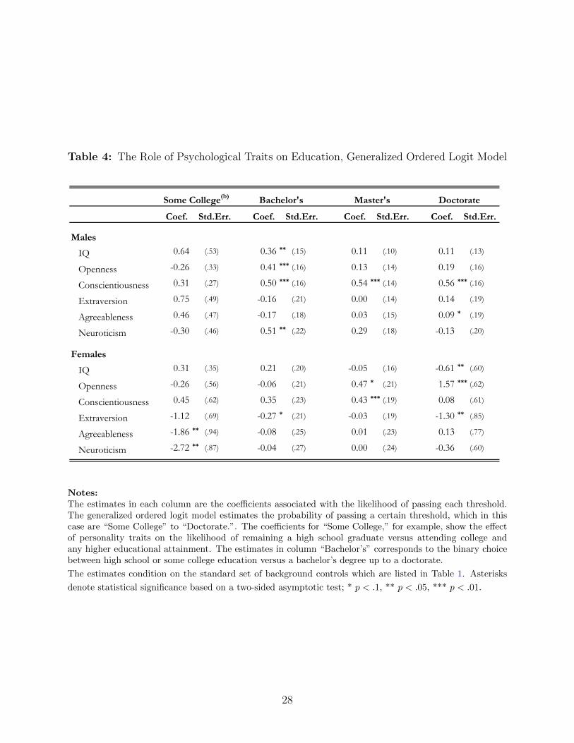
Table 4: The Role of Psychological Traits on Education, Generalized Ordered Logit Model
Some College(b)
Coef. Std.Err. Coef. Std.Err. Coef. Std.Err. Coef. Std.Err.
Males
IQ 0.64 (.53) 0.36 ** (.15) 0.11 (.10) 0.11 (.13)
Openness -0.26 (.33) 0.41 *** (.16) 0.13 (.14) 0.19 (.16)
Conscientiousness 0.31 (.27) 0.50 *** (.16) 0.54 *** (.14) 0.56 *** (.16)
Extraversion 0.75 (.49) -0.16 (.21) 0.00 (.14) 0.14 (.19)
Agreeableness 0.46 (.47) -0.17 (.18) 0.03 (.15) 0.09 * (.19)
Neuroticism -0.30 (.46) 0.51 ** (.22) 0.29 (.18) -0.13 (.20)
Females
IQ 0.31 (.35) 0.21 (.20) -0.05 (.16) -0.61 ** (.60)
Openness -0.26 (.56) -0.06 (.21) 0.47 * (.21) 1.57 *** (.62)
Conscientiousness 0.45 (.62) 0.35 (.23) 0.43 *** (.19) 0.08 (.61)
Extraversion -1.12 (.69) -0.27 * (.21) -0.03 (.19) -1.30 ** (.85)
Agreeableness -1.86 ** (.94) -0.08 (.25) 0.01 (.23) 0.13 (.77)
Neuroticism -2.72 ** (.87) -0.04 (.27) 0.00 (.24) -0.36 (.60)
DoctorateBachelor's Master's
Notes:The estimates in each column are the coefficients associated with the likelihood of passing each threshold.The generalized ordered logit model estimates the probability of passing a certain threshold, which in thiscase are “Some College” to “Doctorate.”. The coefficients for “Some College,” for example, show the effectof personality traits on the likelihood of remaining a high school graduate versus attending college andany higher educational attainment. The estimates in column “Bachelor’s” corresponds to the binary choicebetween high school or some college education versus a bachelor’s degree up to a doctorate.
The estimates condition on the standard set of background controls which are listed in Table 1. Asterisks
denote statistical significance based on a two-sided asymptotic test; * p < .1, ** p < .05, *** p < .01.
28
3.5 The Rate of Return to Schooling
Now that we have established that psychological traits determine educational choice, we
can ask how education translates into lifetime earnings. One common way of summarizing
this information is through the internal rate of return. The rate of return to education is
computed from the estimates of the earnings equations (Equation (1) for ages t = 18, ..., 75).
Because we have complete life-cycle earnings data, we do not have to impose the standard
procedures developed by Becker and Chiswick (1966) and Mincer (1974) to use cross sectional
data to estimate life-cycle rates of return.30 Indeed, we test and reject the adequacy of the
widely-used Mincer specification. Instead of relying on years of schooling as our outcome
variable, we contrast different levels of education in pairwise comparisons. This yields a
richer picture of the different trade-offs that individuals face when choosing one education
level over another.
Furthermore, we show a drastic departure from the traditional rate-of-return analysis,
due to the interactions we have established in Section 3.3. The rate of return to education
is significantly higher for men who are highly extroverted, conscientious, and who score low
on Openness and emotional stability.
We first discuss what the Mincer estimates would be for the Terman sample, and then
contrast it to pairwise internal rates of return for males. Then we show by how much the rate
of return varies by personality traits and IQ. Finally, we turn to the effect of education on
women’s earnings, decomposing the effects on own earnings and on their husbands’ earnings.
All estimates control for the variables of Table 1.
3.5.1 The Mincer Coefficient
Most rates of return that are presented in the literature are not actually estimates of the
internal rate of return. It is common practice to estimate a Mincer equation and interpret
the coefficient on years of schooling as the rate of return. Even though the Terman data
30Heckman et al. (2006, 2008) review the literature which is based on this approach.
29
are longitudinal, one can estimate the Mincer equation as if the data were cross-sectional.
Regressing log wages on years of schooling, experience, and its square, the Terman Mincer
rate of return for males is 7.5%. For women, it is 6.0%, and for combined earnings with their
husbands it is only 3.6%.31 We will see that these rates are masking a lot of different returns
that can be observed for the different education levels.
3.5.2 The IRR for Men
The average treatment effect of education level j vs k at each age t corresponds to νt,j − νt,k
from Eq. (1). Since the treatment effect of education is a function of the psychological traits,
as shown in Section 3.3, we report here the average treatment effect for men with average
scores on all personality traits and average IQ of the sample.32
The pairwise estimates of the average treatment effects are plotted in Fig. 7. Schooling
always has a negative effect on annual earnings in the early years of a working life since
individuals who are obtaining more education are still in school while their peers with less
education are already out of school and working. The effect of education is substantial during
the prime working years, a standard result in the literature (see Becker, 1964).
The IRRs and Net Present Values (NPVs) corresponding to the estimated average effects
are listed in each sub-graph.33 In principle, an IRR should be compared to the market interest
rate to determine the optimality of schooling.34 This comparison ignores the dynamic aspect
31For this comparison, all observations in the treatment-estimation sample are used, ages 18-65, as if theywere from a cross-section. Years of schooling are imputed from degrees and experience is approximated bysubtracting six and the number of years of schooling from the participants current age, as is customary.Then, log wages are regressed on years of schooling and experience, and its square, as well as the set ofpsychological traits and background variables as in our standard estimation.
32Note that in the limit, the average treatment effect of education as estimated from Eq. (1) is equal tothe estimates from Eq. (2), as the personality traits and IQ are normalized to have mean zero.
33The IRR are computed in the traditional fashion suggested by Becker (1964). Even though Becker(1964) and Heckman et al. (2006, 2008) used after-tax earnings, other authors tend to use pre-tax earnings.Therefore, the results here are for earnings after tuition, but before tax. The corresponding figures andtables for after-tax earnings can be found in Web Appendix C, Section C.5.
34The “nonlinear” pattern of some of the pairwise IRRs is not as counterintuitive as it might seem. Forexample, if for males the return of a master’s degree versus a bachelor’s degree is almost zero at -1.1%, andthe IRR of a doctorate degree versus a master’s is 11.5%, one might initially expect the IRR of a doctorateversus a bachelor’s to be similar to 11%. The graphs of pairwise treatment effects are helpful for an intuitiveunderstanding. The IRR of a doctorate over a bachelor’s is the result of a sizeable positive treatment effect
30

of schooling and the sequential revelation of uncertainty.35 Our analysis is explicitly ex-post
and considers rates of return in a static setting.
The pairwise treatment effects are clearly different from each other and can not be sum-
marized in a single “rate of return” as one would obtain from the Mincer coefficient.
In comparison to having a high school diploma, obtaining a bachelor’s degree increases
the Terman males’ earnings by $349,677 over a lifetime, if the difference in earnings is
discounted at 3%. The corresponding IRR is 11.8%. This estimate implies that even for the
highly talented Terman men with IQs above 140, going to school substantially contributed
to increasing their lifetime earnings, and the rate of return to this investment exceeds that
of the return on equity.36
Even though the category of “some college” is a rather heterogeneous one, attending
college (without obtaining a degree) increases the Terman men’s earnings once we hold their
traits constant. The levels of the average treatment effects are similar to those of a bachelor’s
degree, with a slightly smaller investment as well as a lower return later in life. This leads
to an IRR which is still relatively high at 7.8%.
The rates of return for a master’s degree or a doctoral degree in comparison to a high
school diploma are lower—because the investment periods for obtaining these degrees are
longer. The IRRs are 8.1% for a master’s degree and 8.9% for a doctoral degree over a high
school diploma. Note that at almost identical rates of return, the doctoral degree neverthe-
less leads to much higher discounted earnings gains than the master’s degree ($475,022 vs
$279,808).
from age 40 onwards, offset by an initial investment period during which the treatment effect of educationis negative. Yet when comparing men with a doctorate degree to men with a master’s, both groups havehigh foregone earnings during the long time spent in school. The difference in earnings between them isvery small during this period, making the investment cost of a doctorate versus a master’s almost nil. Thedoctorates will, however, have much greater earnings later in life. The return to investment will be largebecause a large payoff is contrasted to a small investment cost.
35See for example Heckman et al. (2006) for a discussion of the problems and particularities associatedwith sequential resolution of uncertainty. The option value of schooling has been analyzed, for example, byHeckman and Urzua (2008).
36For example, the S&P 500 annualized return from 1928 to 1985 (when the Terman men were on average18–75 years old), is about 6%.
31
The absolute treatment effects of incremental improvements, such as bachelor’s degree
over “some college”, or doctorate over master’s, are relatively small. But since these small
gains can be had at an even smaller cost, the resulting rates of returns are substantial (15.0%
and 11.9%).
In comparison to having a bachelor’s degree, having a master’s degree has almost no
return, and the treatment effect is negative for many years. The IRR is actually negative
at -2.4%. For the person with average levels of all psychological traits, obtaining a doctoral
degree over a bachelor’s degree increases increase lifetime earnings, but only by an NPV
of $124.346). Even in a high ability group, education adds skills that are valued on the
marketplace. The returns to schooling are real, and ability bias cannot be responsible for
the type of returns we find.
32

Figure 7: Pairwise Average Treatment Effects on Earnings, Males
IRR = 8.1CI = [−19, 16.1]NPV = 73.201
IRR = 12.2CI = [5.5, 17.4]NPV = 358.977
IRR = 8.5CI = [4, 12.4]NPV = 300.061
IRR = 9.1CI = [5.6, 11.8]NPV = 475.915
Some College vs High School Bachelor's vs High School
Master's vs High School Doctorate vs High School
−20
0
20
40
60
80
100
−20
0
20
40
60
80
100
20 30 40 50 60 70 20 30 40 50 60 70Age
Trea
tmen
t E
ffec
t, 1
,000 U
SD
Some Coll. Bachelor Master Doctorate Some Coll. Bachelor Master Doctorate
High School 8.1 12.2 8.5 9.1 73.2 359.0 300.1 475.9[-19.0, 16.1] [5.5, 17.4] [4.0, 12.4] [5.6, 11.8] [-170, 302] [100, 571] [55, 517] [255, 710]
Some College 15.3 8.7 9.4 287.5 228.6 404.5[4.2, 23.6] [4.5, 14.5] [6.0, 13.1] [95, 486] [30, 459] [214, 662]
Bachelor -1.1 5.8 -57.2 118.7[-12.0, 49.6] [1.7, 12.4] [-252, 175] [-31, 371]
Master 11.5 177.7[-2.0, 22.4] [-5, 427]
IRR NPV
Notes: Treatment effects from Eq. (2), evaluated for a person with average personality traits, and 95% confidence bands
from 200 bootstrap draws. Earnings are annual earnings after tuition in 2010 U.S. Dollars. The covariates are IQ, factor
scores for personality traits, parental background, family environment, early childhood health and 1922 health information,
and controls for WWII and cohort.
33
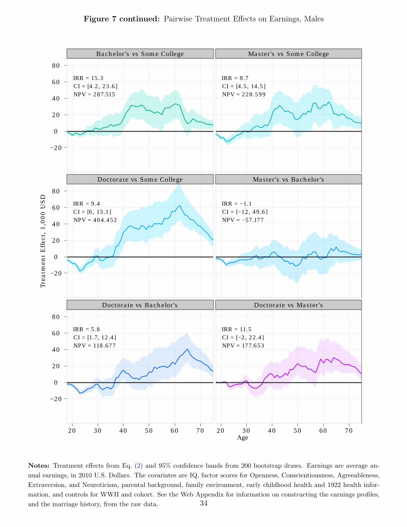
Figure 7 continued: Pairwise Treatment Effects on Earnings, Males
IRR = 15.3CI = [4.2, 23.6]NPV = 287.515
IRR = 8.7CI = [4.5, 14.5]NPV = 228.599
IRR = 9.4CI = [6, 13.1]NPV = 404.452
IRR = −1.1CI = [−12, 49.6]NPV = −57.177
IRR = 5.8CI = [1.7, 12.4]NPV = 118.677
IRR = 11.5CI = [−2, 22.4]NPV = 177.653
Bachelor's vs Some College Master's vs Some College
Doctorate vs Some College Master's vs Bachelor's
Doctorate vs Bachelor's Doctorate vs Master's
−20
0
20
40
60
80
−20
0
20
40
60
80
−20
0
20
40
60
80
20 30 40 50 60 70 20 30 40 50 60 70Age
Trea
tmen
t E
ffec
t, 1
,000 U
SD
Notes: Treatment effects from Eq. (2) and 95% confidence bands from 200 bootstrap draws. Earnings are average an-
nual earnings, in 2010 U.S. Dollars. The covariates are IQ, factor scores for Openness, Conscientiousness, Agreeableness,
Extraversion, and Neuroticism, parental background, family environment, early childhood health and 1922 health infor-
mation, and controls for WWII and cohort. See the Web Appendix for information on constructing the earnings profiles,
and the marriage history, from the raw data. 34

3.5.3 The IRR for Women
The women in the Terman sample belonged to a generation in which the role of the woman
was still mainly that of a homemaker, mother, and wife (see Goldin, 1992). Society defined
very strictly what type of occupations were deemed “suitable” for a woman, and a woman’s
freedom to choose her career or define her own lifestyle was not what it is today. Thus,
we should expect a high share of housewives among the Terman women. About half of the
Terman women did not engage in remunerated activity, despite their extraordinary abilities
and talents.
A woman was more likely to be in gainful employment and less likely to be married if she
had obtained higher levels of education than a Bachelor’s degree, as one can see in Fig. 8.
Whether this relationship between education and labor supply or marital status is causal is
far from clear. For example, a highly educated woman might have chosen to focus her energy
on a career early on, and with own earnings would have been less dependent on finding a
husband. Also, her high education and career aspirations may have made her less attractive
as a marriage partner. It is also possible that causality moves in the other direction. For
example, she might not have found a husband initially, and thus decided to obtain more
schooling in order to support herself. A richer model of decision making is required for
women than for men in order to make causal statements.
Since so many women of this cohort were mainly housewives and did not earn a market
wage, they might gain through education by finding a better match, a husband with higher
educational achievement, and thus increase their potential family earnings. In fact, the
correlation of the Terman women’s years of education with their husband’s (for those who
are married) is .36. We decompose the treatment effect of education for women into its effect
on their own earnings and on their husband’s earnings (which is the effect through marriage).
The combined effect will be the sum of the two, or the treatment effect of education on family
earnings. The decomposition is illustrated graphically in Fig. 9.
The gains through marriage, shown in blue, are positive for women with a bachelor’s
35

Figure 8: Women’s Labor Market Participation and Marriage Histories
(a) Labor Market Participation
0.2
.4.6
.81
Shar
e o
f W
om
en w
ith
Po
siti
ve E
arn
ings
20 30 40 50 60 70
Age
Doctorate (24) Master's (96)Bachelor's (182) High School(130)
(b) Married Status
0.2
.4.6
.81
Shar
e o
f W
om
en M
arri
ed
20 30 40 50 60 70
Age
Doctorate (24) Master's (96)Bachelor's (182) High School(130)
Notes: Observation counts are given in parentheses. The indicator for employment is given by positive own
earnings. The indicator for being married is given at each age, and excludes those who are currently married
but separated.
The education categories refer to the highest educational level the subjects attained in life. See the Web
Appendix for other graphs, as well as information on building the earnings profiles, and the marriage history,
from the raw data.
36
degree over high school. Yet for education levels beyond the bachelor’s, higher education is
associated with slightly lower earnings through marriage. The more highly educated women
are less likely to be married, and thus lose the opportunity to bolster their own earnings with
their husband’s. In the case of women with a Master’s degree, the negative effect is clearly
related to lower probability of being married - as Fig. 8 shows. A woman’s propensity to
be married is much lower for women with a master’s as opposed to a bachelor’s degree or
high school diploma. Most interestingly, the exceptional women who obtained a Doctorate
degree did not suffer significantly in the marriage market, as one might have anticipated.
Even though they were significantly less likely to be married, when they were married their
husbands had higher-than-average earnings, so overall the impact of their high education on
the returns to marriage are not statistically different from zero. Figure 10 explores these
different effects: It shows two counterfactual treatment effects of education on the women’s
gains through marriage. In green, the solid line shows the effect of education on the quality
of matches. It assumes that all women in the sample were married (marriage propensity of
1), and education is allowed to affect only husband’s earnings. For women with a bachelor’s
or doctorate degree, education improves match quality. Women with a master’s were not
able to find higher-earning husbands than less-educated women, leading to a negative return
through match quality. The second counterfactual, represented by the purple dashed line,
assumes that once married, the earnings through husbands were equal. Education affects the
marriage propensity only. Clearly, marriage prospects declined increasingly with education
past a bachelor’s degree. The lower marriage propensity outweighs the effect of education
on match quality, leading to negative returns to education through husbands, as seen in the
blue shade in Fig. 9 .
Women improved their own earnings by obtaining post-graduate education (see the
pink shaded areas). The treatment effect of a master’s degree is positive but remains small
and is not statistically significantly different from zero. For women with a doctorate degree,
the returns to education are substantial, and even higher in absolute levels and IRRs than
37

men’s.
The combined effect of education on family earnings is shown in the solid black line,
and the corresponding IRRs are shown in the box. The treatment effect on family earnings
is dominated by the very large effect on their own earnings for women with a doctoral degree
— it completely washes out the slightly negative effect that education has on husband’s
earnings. Even though family earnings are not precisely estimated age-by-age, the treatment
effect on own earnings is (not shown). Clearly, these women were very special cases. They
worked in high-ranking jobs, had high earnings, and did not rely on their husbands to provide
their earnings. Unfortunately, since there are only 24 women in the sample who obtained a
doctoral degree,37 the treatment effects are relatively imprecisely determined.
The returns to education in terms of family earnings are also positive for women with
a bachelor’s degree, because they benefit from the marriage market. For women with a
master’s, the rate of return is in fact negative, because the return through own earnings is
not enough to offset the losses in the marriage market.38
In the lifetimes of the Terman cohort, women’s opportunities to increase their earnings
through education were more limited for women than they were for men. Women’s own
earnings mostly fell short of the earnings of men with the same level of education and ability;
not only due to the choice of occupation, but also within occupation. At the same time,
marriage prospects were not always boosted by higher education, and only increased earnings
sufficiently for women with a college education to offset their smaller market returns. For
them, the rates of return to education were similar to those of Terman men.
37There were 26 women in the overall sample, but we restrict the treatment effect analysis to thoseobservations with complete earnings histories.
38The rate of return of a master’s degree over the high school diploma cannot be computed because thereare multiple crossings with the zero line, and also there might simply not exist a rate of return that wouldset the net present value of this investment to zero.
38
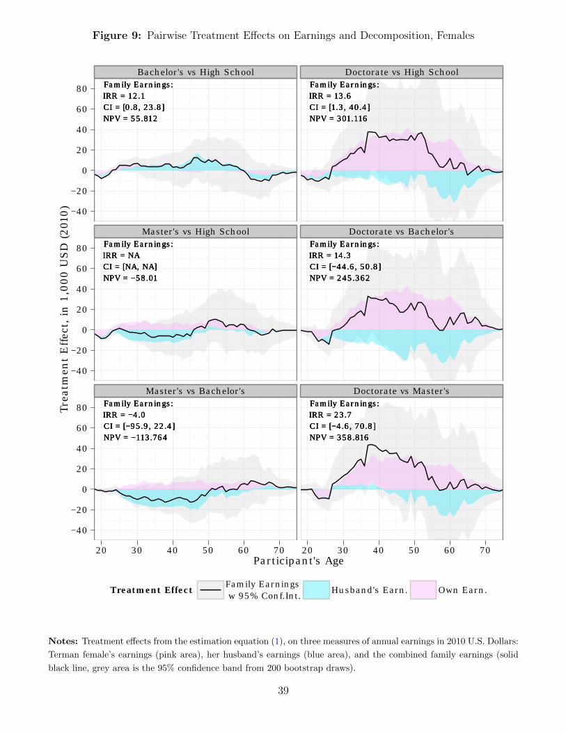
Figure 9: Pairwise Treatment Effects on Earnings and Decomposition, Females
Family Earnings: IRR = 12.1CI = [0.8, 23.8]NPV = 55.812
Family Earnings: IRR = 12.1CI = [0.8, 23.8]NPV = 55.812
Family Earnings: IRR = 12.1CI = [0.8, 23.8]NPV = 55.812
Family Earnings: IRR = 13.6CI = [1.3, 40.4]NPV = 301.116
Family Earnings: IRR = 13.6CI = [1.3, 40.4]NPV = 301.116
Family Earnings: IRR = 13.6CI = [1.3, 40.4]NPV = 301.116
Family Earnings: IRR = NACI = [NA, NA]NPV = −58.01
Family Earnings: IRR = NACI = [NA, NA]NPV = −58.01
Family Earnings: IRR = NACI = [NA, NA]NPV = −58.01
Family Earnings: IRR = 14.3CI = [−44.6, 50.8]NPV = 245.362
Family Earnings: IRR = 14.3CI = [−44.6, 50.8]NPV = 245.362
Family Earnings: IRR = 14.3CI = [−44.6, 50.8]NPV = 245.362
Family Earnings: IRR = −4.0CI = [−95.9, 22.4]NPV = −113.764
Family Earnings: IRR = −4.0CI = [−95.9, 22.4]NPV = −113.764
Family Earnings: IRR = −4.0CI = [−95.9, 22.4]NPV = −113.764
Family Earnings: IRR = 23.7CI = [−4.6, 70.8]NPV = 358.816
Family Earnings: IRR = 23.7CI = [−4.6, 70.8]NPV = 358.816
Family Earnings: IRR = 23.7CI = [−4.6, 70.8]NPV = 358.816
Bachelor's vs High School Doctorate vs High School
Master's vs High School Doctorate vs Bachelor's
Master's vs Bachelor's Doctorate vs Master's
−40
−20
0
20
40
60
80
−40
−20
0
20
40
60
80
−40
−20
0
20
40
60
80
20 30 40 50 60 70 20 30 40 50 60 70Participant's Age
Trea
tmen
t E
ffec
t, in
1,0
00 U
SD
(201
0)
Treatment Effect Family Earnings w 95% Conf.Int.
Husband's Earn. Own Earn.
Notes: Treatment effects from the estimation equation (1), on three measures of annual earnings in 2010 U.S. Dollars:
Terman female’s earnings (pink area), her husband’s earnings (blue area), and the combined family earnings (solid
black line, grey area is the 95% confidence band from 200 bootstrap draws).
39
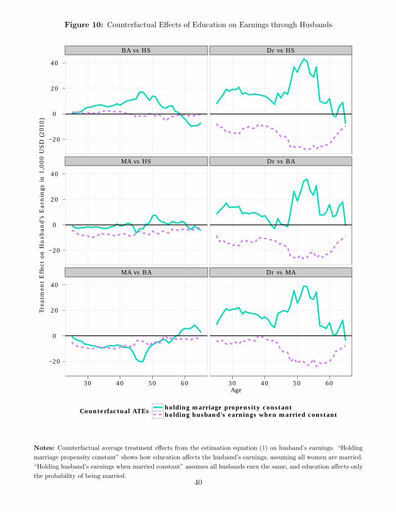
Figure 10: Counterfactual Effects of Education on Earnings through Husbands
BA vs HS Dr vs HS
MA vs HS Dr vs BA
MA vs BA Dr vs MA
−20
0
20
40
−20
0
20
40
−20
0
20
40
30 40 50 60 30 40 50 60Age
Trea
tmen
t E
ffec
t on
Hu
sban
d's
Ear
nin
gs in
1,0
00 U
SD
(201
0)
Counterfactual ATEs holding marriage propensity constantholding husband's earnings when married constant
Notes: Counterfactual average treatment effects from the estimation equation (1) on husband’s earnings. “Holding
marriage propensity constant” shows how education affects the husband’s earnings, assuming all women are married.
“Holding husband’s earnings when married constant” assumes all husbands earn the same, and education affects only
the probability of being married.40

4 Conclusion
This paper estimates the effects of personality traits and IQ on lifetime earnings of the
high-achieving men and women of the Terman study.
Personality traits and IQ affect the levels of earnings, especially in the prime working
years. They also affect educational sorting and thus command an indirect effect on lifetime
earnings. Furthermore, their effects on lifetime earnings are a function of educational at-
tainment. Therefore, the treatment effect of schooling is a function of personality traits. By
the unique access to the full lifetime earnings histories, these heterogeneous effects can be
disentangled - in an age-by-age estimation, they may fail to be statistically significant.
Psychological traits are priced directly in the marketplace for men, but not for women.
Men gain from traits such as Conscientiousness, Extraversion, and IQ. Women with up to a
Bachelor’s degree are able to gain from Extraversion by matching to higher-earning partners.
The presented estimates of the internal rate of return to education do not rely on the
strong assumptions that are standard in the literature to estimate the “rates of return.”
Instead, the returns are based on causal effects, obtained by matching on an unusually
extensive list of covariates, including IQ and personality. The analysis of the returns to
education for persons at the high end of the IQ distribution is unique.
The returns for the Terman men can be sizeable. For women at education levels below
the doctoral level, the rates of return are low. Women with a college education gain through
sorting in the marriage market. Women with a doctorate degree have very high earnings on
their own, and their rates of return are even higher than those of men.
41
References
Almlund, M., A. Duckworth, J. J. Heckman, and T. Kautz (2011). Personality psychology
and economics. In E. A. Hanushek, S. Machin, and L. Woßmann (Eds.), Handbook of the
Economics of Education, Volume 4, pp. 1–181. Amsterdam: Elsevier.
Baron, J. D. and D. Cobb-Clark (2010). Are Young Peoples Educational Outcomes Linked
to their Sense of Control? Discussion Paper 4907, Institute for the Study of Labor (IZA),
Bonn.
Bartlett, M. (1937). The Statistical Conception of Mental Factors. British Journal of Psy-
chology 1 (28), 97–104.
Becker, G. S. (1964). Human Capital: A Theoretical and Empirical Analysis, With Special
Reference to Education. New York: National Bureau of Economic Research.
Becker, G. S. and B. R. Chiswick (1966, March). Education and the distribution of earnings.
American Economic Review 56 (1/2), 358–369.
Becker, G. S., E. M. Landes, and R. T. Michael (1977). An economic analysis of marital
instability. Journal of Political Economy 85 (6), 1141–1187.
Bolck, A., M. Croon, and J. Hagenaars (2004, February). Estimating Latent Structure
Models with Categorical Variables: One-Step Versus Three-Step Estimators. Political
Analysis 12 (1), 3–27.
Borghans, L., B. H. H. Golsteyn, J. J. Heckman, and J. E. Humphries (2011). Identification
problems in personality psychology. Personality and Individual Differences 51 (Special
Issue on Personality and Economics), 315–320. E. Ferguson, J.J. Heckman, and P. Corr,
editors.
Croon, M. (2002). Using Predicted Latent Scores in General Latent Structure Models. In
42
G. A. Marcoulides and I. Moustaki (Eds.), Latent Variable and Latent Structure Models,
Chapter 10, pp. 195–223. Lawrence Erlbaum Associates, Inc.
Friedman, H. S. (2000). Long-term relations of personality and health: Dynamism, mecha-
nisms, tropisms. Journal of Personality 68 (6), 1089–1107.
Friedman, H. S. (2008, July). The multiple linkages of personality and disease. Brain,
Behavior, and Immunity 22 (5), 668–675.
Friedman, H. S., P. H. Hawley, and J. S. Tucker (1994). Personality, health, and longevity.
Current Directions in Psychological Science 3 (2), 37–41.
Friedman, H. S., J. S. Tucker, J. E. Schwartz, L. R. Martin, C. Tomlinson-Keasey, D. L.
Wingard, and M. H. Criqui (1995). Childhood conscientiousness and longevity: Health
behaviors and cause of death. Journal of Personality and Social Psychology 68 (4), 696–
703.
Friedman, H. S., J. S. Tucker, J. E. Schwartz, C. Tomlinson-Keasey, L. R. Martin, D. L.
Wingard, and M. H. Criqui (1995). Psychosocial and behavioral predictors of longevity:
The aging and death of the “Termites.”. American Psychologist 50 (2), 69–78.
Friedman, H. S., J. S. Tucker, C. Tomlinson-Keasey, J. E. Schwartz, D. L. Wingard, and
M. H. Criqui (1993a). Does childhood personality predict longevity? Journal of Person-
ality and Social Psychology 65 (1), 176–185.
Friedman, H. S., J. S. Tucker, C. Tomlinson-Keasey, J. E. Schwartz, D. L. Wingard, and
M. H. Criqui (1993b, July). Does childhood personality predict longevity? Journal of
personality and social psychology 65 (1), 176–85.
Gladwell, M. (2008, November). Outliers: the story of success. New York, NY: Little, Brown
and Company.
43

Goldberg, L. R. (1993). The structure of phenotypic personality traits. American Psychol-
ogist 48 (1), 26–34.
Goldin, C. (1992). Understanding the Gender Gap: An Economic History of American
Women. NBER Series on Long-Term Factors in Economic Development, Oxford University
Press.
Goodwin, R. D. and H. S. Friedman (2006, September). Health status and the five-factor
personality traits in a nationally representative sample. Journal of health psychology 11 (5),
643–54.
Hamermesh, D. S. (1984). Life-cycle effects on consumption and retirement. Journal of
Labor Economics 2 (3), 353–370.
Heckman, J. J., L. J. Lochner, and P. E. Todd (2006). Earnings equations and rates of return:
The Mincer equation and beyond. In E. A. Hanushek and F. Welch (Eds.), Handbook of
the Economics of Education, Chapter 7, pp. 307–458. Amsterdam: Elsevier.
Heckman, J. J., L. J. Lochner, and P. E. Todd (2008, Spring). Earnings functions and rates
of return. Journal of Human Capital 2 (1), 1–31.
Heckman, J. J., L. Malofeeva, R. Pinto, and P. A. Savelyev (2011). Understanding the
mechanisms through which an influential early childhood program boosted adult outcomes.
Unpublished manuscript, University of Chicago, Department of Economics (first draft,
2008). Under revision, American Economic Review.
Heckman, J. J. and R. Robb (1985). Using longitudinal data to estimate age, period and
cohort effects in earnings equations. In W. M. Mason and S. E. Fienberg (Eds.), Cohort
Analysis in Social Research: Beyond the Identification Problem. New York: Springer-
Verlag.
44
Heckman, J. J., S. Schennach, and B. Williams (2011). Matching with error-laden covariates.
Unpublished manuscript, University of Chicago, Department of Economics.
Heckman, J. J. and S. Urzua (2008, June). The option value of educational choices and
the rate of return to educational choices. Unpublished manuscript, University of Chicago.
Presented at the Cowles Foundation Structural Conference, Yale University.
Hogan, R. and J. Hogan (2007). Hogan Personality Inventory Manual (3rd ed.). Tulsa, OK:
Hogan Assessment Systems.
Hoshino, T. and K. Shigemasu (2008, March). Standard Errors of Estimated Latent Variable
Scores With Estimated Structural Parameters. Applied Psychological Measurement 32 (2),
181–189.
Leibowitz, A. (1974, March/April). Home investments in children. Journal of Political
Economy 82 (2), S111–S131.
Lodi-Smith, J., J. Jackson, T. Bogg, K. Walton, D. Wood, P. Harms, and B. W. Roberts
(2010). Mechanisms of health: Education and health-related behaviours partially mediate
the relationship between conscientiousness and self-reported physical health. Psychological
Health 25 (3), 305–319.
Marks, G. R. and S. K. Lutgendorf (1999, May). Perceived Health Competence and Person-
ality Factors Differentially Predict Health Behaviors in Older Adults. Journal of Aging
and Health 11 (2), 221–239.
Martin, L. R. and H. S. Friedman (2000). Comparing personality scales across time: An
illustrative study of validity and consistency in life-span archival data. Journal of Person-
ality 68 (1), 85–110.
Martin, L. R., H. S. Friedman, K. M. Clark, and J. S. Tucker (2005). Longevity following
the experience of parental divorce. Social Science and Medicine 61 (10), 2177–2189.
45
Martin, L. R., H. S. Friedman, and J. E. Schwartz (2007). Personality and mortality risk
across the life span: The importance of conscientiousness as a biopsychosocial attribute.
Health Psychology 26 (4), 428–436.
Martin, L. R., H. S. Friedman, J. S. Tucker, C. Tomlinson-Keasey, M. H. Criqui, and J. E.
Schwartz (2002). A life course perspective on childhood cheerfulness and its relation to
mortality risk. Personality and Social Psychology Bulletin 28 (9), 1155–1165.
Michael, R. T. (1976). Factors affecting divorce: A study of the Terman sample. NBER
Working Papers 147, National Bureau of Economic Research, Inc.
Mincer, J. (1974). Schooling, Experience and Earnings. New York: Columbia University
Press for National Bureau of Economic Research.
Mokdad, A. H., J. S. Marks, D. F. Stroup, and J. L. Gerberding (2004, March). Actual
causes of death in the United States, 2000. JAMA : The Journal of the American Medical
Association 291 (10), 1238–45.
Muller, G. and E. Plug (2004). Estimating the Effect of Personality on Male-Female Earnings.
Tinbergen Institute Discussion Paper 087/3.
Roberts, B. W., K. E. Walton, and T. Bogg (2005). Conscientiousness and Health Across
the Life Course. Review of General Psychology 9 (2), 156–168.
Savelyev, P. (2011). Conscientiousness, education, and longevity of high-ability individuals.
Unpublished manuscript, Vanderbilt University, Department of Economics.
Schwartz, J. E., H. S. Friedman, J. S. Tucker, C. Tomlinson-Keasey, D. L. Wingard, and
M. H. Criqui (1995, September). Sociodemographic and psychosocial factors in childhood
as predictors of adult mortality. American Journal of Public Health 85 (9), 1237–1245.
Sears, R. R. (1984). Handbook of longitudinal research, Volume 1, Chapter The Terman
gifted children study., pp. 398–414. New York: Praeger.
46
Terman, L. M., B. T. Baldwin, E. Bronson, J. C. DeVoss, F. Fuller, T. Lee Kelley, M. Lima,
H. Marshall, A. H. Moore, A. S. Raubenheimer, G. M. Ruch, R. L. Willoughby, J. Ben-
son Wyman, and D. Hazeltine Yates (1925). Genetic Studies of Genius: Mental and
Physical Traits of a Thousand Gifted Children, Volume 1. Stanford University, CA: Stan-
ford University Press.
Terman, L. M. and R. R. Sears (2002a). The Terman Life-Cycle Study of Children with High
Ability, 1922-1986, Volume 1, 1922-1928. Ann Arbor, MI: Inter-University Consortium
for Political and Social Research.
Terman, L. M. and R. R. Sears (2002b). The Terman Life-Cycle Study of Children with High
Ability, 1922-1986, Volume 3, 1950-1986. Ann Arbor, MI: Inter-University Consortium
for Political and Social Research.
Terman, L. M., R. R. Sears, L. J. Cronbach, and P. S. Sears (2002a). The Terman Life-Cycle
Study of Children with High Ability, 1922-1986, Volume 2, 1936-1945. Ann Arbor, MI:
Inter-University Consortium for Political and Social Research.
Terman, L. M., R. R. Sears, L. J. Cronbach, and P. S. Sears (2002b). The Terman Life-Cycle
Study of Children with High Ability, 1922-1986, Volume 4, 1991, Parts 69 and 70. Ann
Arbor, MI: Inter-University Consortium for Political and Social Research.
Thomson, G. H. (1938). Methods of Estimating Mental Factors. Nature 141 (Feb. 5), 246.
Thurstone, L. (1935). The vectors of mind. Chicago, IL: University of Chicago Press.
Tomes, N. (1981, April). A model of fertility and children’s schooling. Economic In-
quiry 19 (2), 209.
Tucker, J. S., H. S. Friedman, J. E. Schwartz, M. H. Criqui, C. Tomlinson-Keasey, D. L.
Wingard, and L. R. Martin (1997). Parental divorce: Effects on individual behavior and
longevity. Journal of Personality and Social Psychology 73 (2), 381–391.
47

Tucker, J. S., H. S. Friedman, D. L. Wingard, and J. E. Schwartz (1996). Marital history
at midlife as a predictor of longevity: Alternative explanations to the protective effect of
marriage. Health Psychology 15 (2), 94–101.
Tucker, J. S., J. E. Schwartz, K. M. Clark, and H. S. Friedman (1999). Age-related changes
in the associations of social network ties with mortality risk. Psychology and Aging 14 (4),
564–571.
Weiss, A. and P. T. Costa (2005). Domain and facet personality predictors of all-cause
mortality among Medicare patients aged 65 to 100. Psychosomatic medicine 67 (5), 724–
33.
Williams, R. (2006). Generalized ordered logitpartial proportional odds models for ordinal
dependent variables. The Stata Journal 6 (1), 58–82.
48