Person Detection using RGB-D Sensor and

Thermo Camera

M. Pecka, V. Kubelka, L. Wagner and K. Zimmermann

April 13, 2016

1 Introduction

Doc. Ing. F. Zlo, CSc. wants1 to reduce the number of students by means ofRobotron [1]. However, the publicly available face detector he has been using sofar produces too many false positive detections (e.g. printed faces on posters).Given a proper calibration of provided sensors, you can augment bare RGBimages with temperature and depth information. Avoid being exterminated byDoc. Ing. Zlo CSc., prove yourself useful and find a way to use the temperatureand depth information to improve the detector so that it detects only facesof real persons. An example of how your algorithm should work is given inFigure 1. Please note that Doc. Ing. Zlo, who might appear in provided data,is not a real person.

2 Solution outline

We have used an RGB-D sensor and thermo camera to record target data intoa set of MAT-files, see Section 4 for details. Your task is to improve the givenface detector, which detects faces only in RGB images; see Section 7 for details.Since the thermo-camera and the depth sensor are also available, it is desirableto enrich the standard color image by temperature and distance of observedfaces. You will find these measurements useful for improving the face detector.However, images provided by the sensors are not the same size nor aligned sincethe sensors are mounted next to each other so they observe the scene fromdifferent viewpoints. Hence, you will need to find the transformation that bindspixels of the images together. See Section 5 for details. Once the transformationamong measurements is known, you are expected to build your own detector on

1Except the use-case of Doc. Ing. Zlo, a precise detector of real persons can be furtherutilized in several ways. It may also serve as a part of a victim detection system, whichis essential for almost all Search&Rescue robots. Or it may be a part of a security videosurveillance system. Last, but not least, it may be useful for interactive robots to detectpeople around them and start a conversation, offer help or some other task. Connected with(known) face recognition, the possibilities are even greater.

1

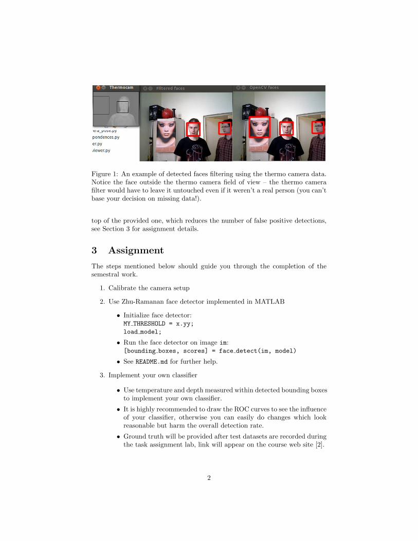
Figure 1: An example of detected faces filtering using the thermo camera data.Notice the face outside the thermo camera field of view – the thermo camerafilter would have to leave it untouched even if it weren’t a real person (you can’tbase your decision on missing data!).

top of the provided one, which reduces the number of false positive detections,see Section 3 for assignment details.

3 Assignment

The steps mentioned below should guide you through the completion of thesemestral work.

1. Calibrate the camera setup

2. Use Zhu-Ramanan face detector implemented in MATLAB

• Initialize face detector:MY THRESHOLD = x.yy;

load model;

• Run the face detector on image im:[bounding boxes, scores] = face detect(im, model)

• See README.md for further help.

3. Implement your own classifier

• Use temperature and depth measured within detected bounding boxesto implement your own classifier.

• It is highly recommended to draw the ROC curves to see the influenceof your classifier, otherwise you can easily do changes which lookreasonable but harm the overall detection rate.

• Ground truth will be provided after test datasets are recorded duringthe task assignment lab, link will appear on the course web site [2].

2

Note, that correctly drawn ROC curve is a compulsory part of your report.Both TP and FP are relative with respect to all ground truth faces in allBAG files – for example: if you have 10 incorrect detections and 50 correctdetections out of 100 ground truth faces, then TP = 0.5 and FP = 0.1).This also means TP can not have values greater than 1 (the best we can dois detect all faces), but FP can surely go beyond 1 (if the detector shows toomuch false faces). A correctly detected face is a bounding box B coveringground truth bounding box B0 by more than 50%, i.e.

B ∩B0

B ∪B0≥ 0.5 (1)

4. Create a PDF file containing only explicit answers to the following ques-tions:

(a) What is the reprojection error of your calibration matrix?Output: Real number from interval [0;∞].

(b) You are given a calibration matrix P of your camera. Let us supposethat you increase the camera resolution two-times (i.e. rows= 2×rows, cols= 2× cols), while its world position is preserved. Calibra-tion matrix of the new camera is H ·P. What is the matrix H ∈ R3×3?Output: Real matrix H ∈ R3×3.

(c) Draw the ROC curve of (i) the provided RGB face detector (withparameters used for your final detector) and (ii) your final RGB-D-Tface detector, with FP ranging from 0 to at least 1.Output: One graph with two ROC curves with FP on hori-zontal axis and TP on the vertical axis.

(d) What is TP for FP = 0.05? (Highest achieved TP will be rewarded bya bottled beer signed by all IRO teachers and personal congratulationof doc. Ing. Zlo, CSc. in front of the whole classroom).Output: Real number from interval [0; 1].

(e) It is obvious that previously defined ROC curves can be identical orthey can touch each other. Is it also possible that one ROC curvestrictly intersects the other (i.e. there is one FP-interval in which thefirst ROC has strictly lower FN and another FP-interval in which thesecond ROC has strictly lower FN)?Output: Binary answer {yes,no}.

(f) Let us take your detector with fixed θ corresponding to FP = 0.05on your testing set consisting of L images with fixed resolution (andlow density of faces). Let us create a new testing set by adding Lbackground images (images without faces) in the same resolution.How does the FP, FN change when detector is evaluated on the newtesting set?Output: Two real numbers N,M ∈ [0;∞] corresponding tothe claim that the resulting false positive is approximatelyN × FP and resulting false negative is approximately M × FN.

3

5. Submit your work

• Your work has to be uploaded to the Upload system. The report issubmitted to task answers. All your codes should be zipped and sub-mitted to task code. Do not include any binary files in the submittedpackage (MAT files...).

4 Sensors and data description

The first sensor is the ASUS Xtion PRO LIVE providing standard color images(640x480 pixels) as well as depth images of the same size (a combination of thesetwo images is denoted as RGB-D). These two images are already calibrated foryou – there is both the RGB and depth information at all pixel coordinates.The depth information is expressed in meters; zero depth indicates no depthinformation at that particular pixel. Depth stands for the Z coordinate of thecorresponding 3D point – a plane parallel with the image sensor will have aconstant value indicated by the depth sensor.

The second sensor is a thermo-camera, namely thermoIMAGER TIM 160from MICRO-EPSILON. This camera captures infrared images (160x120 pix-els), where the value of each pixel is the temperature of the corresponding surfaceobserved by the camera (approximate temperature in our case, emissivity is nottaken into account). In the provided dataset, the temperature is rounded tointegers. Make sure you convert the values into float or double types beforedivision.

These two sensors are attached to a common holder (see Figure 2 for arough idea, the actual setup differs), yet the exact configuration is not known(by the configuration, we mean the rotation and translation of camera opticalcenters). The only known parameter is the RGB-D camera calibration matrixK. This parameter is sufficient – combined with the depth information – toproject each pixel of the RGB-D camera to corresponding 3D space coordinates.That is, for each color-depth image pair, you are able to get 640 × 480 pointsXrgbd = [x, y, z]T that create a colored point-cloud. The images are recordedusing Matlab, therefore the output provided to you are MAT files containing allthe images as matrices. The provided MAT files are zipped into the followingarchives:

• calibration.zip: image topics with the calibration sequence (the hotmetal plate).

• train-lab-i.zip: image topics with real and artificial faces; use these fordetector design. Use the one, where i corresponds to your class number.

• test.zip: same as the previous one, but ground truth will be providedfor this dataset; use it to evaluate your result.

The first MAT file is available on the course web site, the other two will beprovided after the class where this assignment is presented – students of IROwill be involved in the recording of these datasets.

4

Figure 2: The two sensors involved: ASUS Xtion PRO LIVE (top), thermoIM-AGER TIM 160 (bottom).

Each zipped archive contains the following files:

• kinect K.mat: contains the calibration matrix K of the PrimeSense cam-era.

• depth images.mat: Depth data: a matrix of floats of size n × 480 × 640represented the distance in meters.

• rgb images.mat: RGB data: a matrix of bytes of size n× 480× 640× 3,where each triplet of the data represents one RGB point.

• thermo images.mat: Thermo data: a matrix of integers of size n× 120×160 representing the temperature in degrees Celsium.

TECHNICAL NOTE: The sensors generate images with rate higher than80Hz. To keep the bag files reasonably large, we diminished the rate to ap-prox. 3Hz by saving only a subset of all available images. Moreover, we chosethe subset to be as synchronous as possible. Thus, you can consider the tripletsof images to be synchronous keeping in mind that small delays may occur.

TECHNICAL NOTE 2: To get a single image out of the provided MAT file,you have to use the squeeze function like this:image = squeeze(rgb images(i,:,:,:)) .You can visualize the images using imagesc.

Doc. Zlo will choose one representative dataset from those created duringthe labs and make some poor assistant manually create ground truth. You willbe asked to use this ground truth to evaluate your ROC curves and possibly

5

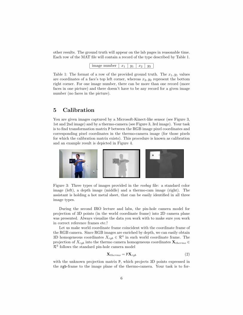
other results. The ground truth will appear on the lab pages in reasonable time.Each row of the MAT file will contain a record of the type described by Table 1.

image number x1 y1 x2 y2

Table 1: The format of a row of the provided ground truth. The x1, y1 valuesare coordinates of a face’s top left corner, whereas x2, y2 represent the bottomright corner. For one image number, there can be more than one record (morefaces in one picture) and there doesn’t have to be any record for a given imagenumber (no faces in the picture).

5 Calibration

You are given images captured by a Microsoft-Kinect-like sensor (see Figure 3,1st and 2nd image) and by a thermo-camera (see Figure 3, 3rd image). Your taskis to find transformation matrix P between the RGB image pixel coordinates andcorresponding pixel coordinates in the thermo-camera image (for those pixelsfor which the calibration matrix exists). This procedure is known as calibrationand an example result is depicted in Figure 4.

Figure 3: Three types of images provided in the rosbag file: a standard colorimage (left), a depth image (middle) and a thermo-cam image (right). Theassistant is holding a hot metal sheet, that can be easily identified in all threeimage types.

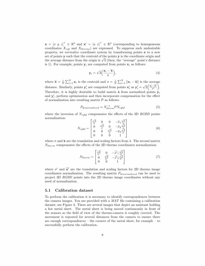
During the second IRO lecture and labs, the pin-hole camera model forprojection of 3D points (in the world coordinate frame) into 2D camera planewas presented. Always visualize the data you work with to make sure you workin correct reference frames etc.!

Let us make world coordinate frame coincident with the coordinate frame ofthe RGB camera. Since RGB images are enriched by depth, we can easily obtain3D homogeneous coordinates Xrgb ∈ R4 in such world coordinate frame. Theprojection of Xrgb into the thermo camera homogeneous coordinates Xthermo ∈R3 follows the standard pin-hole camera model

Xthermo = PXrgb (2)

with the unknown projection matrix P, which projects 3D points expressed inthe rgb-frame to the image plane of the thermo-camera. Your task is to for-

6

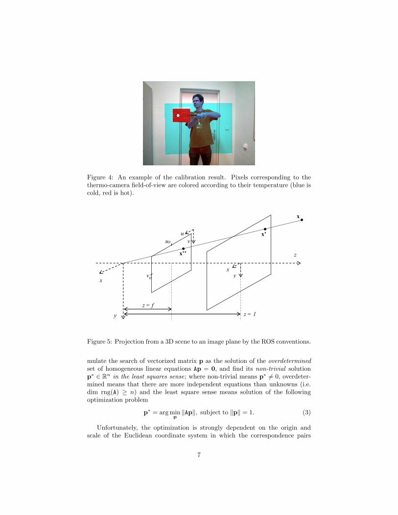
Figure 4: An example of the calibration result. Pixels corresponding to thethermo-camera field-of-view are colored according to their temperature (blue iscold, red is hot).

z

y

x

z = 1

z = f

y x

u

v

x

x’

x’’

u0

v0

Figure 5: Projection from a 3D scene to an image plane by the ROS conventions.

mulate the search of vectorized matrix p as the solution of the overdeterminedset of homogeneous linear equations Ap = 0, and find its non-trivial solutionp∗ ∈ Rn in the least squares sense; where non-trivial means p∗ 6= 0, overdeter-mined means that there are more independent equations than unknowns (i.e.dim rng(A) ≥ n) and the least square sense means solution of the followingoptimization problem

p∗ = arg minp‖Ap‖, subject to ‖p‖ = 1. (3)

Unfortunately, the optimization is strongly dependent on the origin andscale of the Euclidean coordinate system in which the correspondence pairs

7

x = [x y z]> ∈ R3 and x′ = [u v]> ∈ R2 (corresponding to homogeneouscoordinates Xrgb and Xthermo) are expressed. To suppress such undesirableproperty, we normalize coordinate system by transforming points x to a newset of points y such that the centroid of the points y is the coordinate origin andthe average distance from the origin is

√3 (then, the “average” point’s distance

is 1). For example, points yi are computed from points xi as follows:

yi =√

3(xi − x

σ

), (4)

where x = 1N

∑Ni=1 xi is the centroid and σ = 1

N

∑Ni=1 ‖xi − x‖ is the average

distance. Similarly, points y′i are computed from points x′i as y′i =√

2(

x′i−x′

σ′

).

Therefore, it is highly desirable to build matrix A from normalized points yiand y′i, perform optimization and then incorporate compensation for the effectof normalization into resulting matrix P as follows:

Pdenormalized = N−1thermPNrgbd (5)

where the inversion of Nrgbd compensates the effects of the 3D RGBD pointsnormalization:

Nrgbd =

√3σ 0 0 −x1

√3σ

0√3σ 0 −x2

√3σ

0 0√3σ −x3

√3σ

0 0 0 1

(6)

where σ and x are the translation and scaling factors from 4. The second matrixNtherm compensates the effects of the 2D thermo coordinates normalization:

Ntherm =

√2σ′ 0 −x′1

√2σ′

0√2σ′ −x′2

√2σ′

0 0 1

(7)

where σ′ and x′ are the translation and scaling factors for 2D thermo imagecoordinates normalization. The resulting matrix Pdenormalized can be used toproject 3D RGBD points into the 2D thermo image coordinates without anyneed of normalization.

5.1 Calibration dataset

To perform the calibration it is necessary to identify correspondences betweenthe camera images. You are provided with a MAT file containing a calibrationdataset, see Figure 3. There are several images that depict an assistant holdinga hot metal sheet. The metal sheet is being moved continuously in front ofthe sensors so the field of view of the thermo-camera is roughly covered. Themovement is repeated for several distances from the camera to ensure thereare enough correspondences – the corners of the metal sheet, for example – tosuccessfully perform the calibration.

8

We suggest that you go through all the calibration images (using imagesc

and pause) and select just a few (3-5) frames in which the pose of the metalsheet is very different. You can then use ginput to click on the correspondingcorners of the metal sheet in both RGB/Depth and Thermo images. This wayyou get the Xthermo and Xrgb sets, from which you form the A matrix.

6 Reprojection error

In order to find projection matrix P, 3D-2D correspondences need to be iden-tified in the calibration dataset between the RGBD sensor and thermo-camera.Reprojection error stands for average distance between coordinates of the 2Dpoints used for calibration and those obtained by applying projection matrix Pon their 3D counterparts. Therefore, in the ideal case, we would observe thatafter projecting 3D points by our matrix P, they would perfectly coincide withthe original 2D points we used for calibration.

Nevertheless, because of imperfections in the whole calibration chain (imper-fections of lenses, asynchronous image triplets, depth sensor noise, incorrectlymarked correspondences, . . . ) the original 2D points and those obtained byprojecting the 3D points will not fit. That is to be expected and measured bythe reprojection error. In your assignment, use your 3D-2D correspondences toevaluate this error, good result is an average error smaller than 2 pixels (we ex-pect standard euclidean L2 distance). However, be aware of the fact that usingsmall number of (incorrect) correspondences can lead to minimal reprojectionerror (minimum is 6 correspondences that will always lead to – almost – zeroerror) while the P matrix is nonsense. Use at least 10 correspondences, the morethe better.

7 Face detection

7.1 The face detector

The Zhu-Ramanan face detector is a detector based on mixtures of trees witha shared pool of parts, see [4] for details. In its full strength, it provides muchmore information about faces in the image than is needed for our task (e.g.landmark locations and their relative poses). So we slightly altered its output tojust return the smallest bounding box containing all the returned landmarks forevery detected face. Therefore, you can treat the detector as a classifier solvinga binary decision task, with labels y ∈ {F, B} (i.e. Face and Background), onthe set of all rectangles in the image.

7.2 Evaluation of detector quality

A graph depicting the relation between true positives TP(θ) = 1−FN(θ) and falsepositives FP(θ) as a function of classification threshold θ is called ROC curve, seeFigure 6. We also introduced ROC curves during the 6th lab (Bayesian decision

9

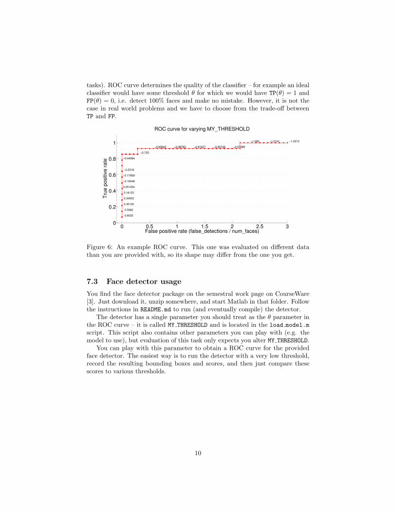
tasks). ROC curve determines the quality of the classifier – for example an idealclassifier would have some threshold θ for which we would have TP(θ) = 1 andFP(θ) = 0, i.e. detect 100% faces and make no mistake. However, it is not thecase in real world problems and we have to choose from the trade-off betweenTP and FP.

0 0.5 1 1.5 2 2.5 30

0.2

0.4

0.6

0.8

1

False positive rate (false_detections / num_faces)

Tru

e p

ositiv

e r

ate

ROC curve for varying MY_THRESHOLD

−0.2518

−0.17959

−0.16546

0.051434

0.16125

0.34503

0.40122

0.5062

0.6533

−0.44394

−0.725

−0.85843 −0.88782 −0.91627 −0.95748 −0.97989

−1.002 −1.0141 −1.0213 −1.0333

Figure 6: An example ROC curve. This one was evaluated on different datathan you are provided with, so its shape may differ from the one you get.

7.3 Face detector usage

You find the face detector package on the semestral work page on CourseWare[3]. Just download it, unzip somewhere, and start Matlab in that folder. Followthe instructions in README.md to run (and eventually compile) the detector.

The detector has a single parameter you should treat as the θ parameter inthe ROC curve – it is called MY THRESHOLD and is located in the load model.m

script. This script also contains other parameters you can play with (e.g. themodel to use), but evaluation of this task only expects you alter MY THRESHOLD.

You can play with this parameter to obtain a ROC curve for the providedface detector. The easiest way is to run the detector with a very low threshold,record the resulting bounding boxes and scores, and then just compare thesescores to various thresholds.

10

References

[1] Bugemos. Robotron. http://bugemos.com/komiksy/Student/2-10.gif.

[2] IRO Team. Task 2 cw page. https://cw.fel.cvut.cz/wiki/courses/

a3m33iro/semestralni_uloha.

[3] Xiangxin Zhu and Deva Ramanan. Face detection, pose esti-mation, and landmark localization in the wild, source codes foriro course. http://ptak.felk.cvut.cz/tradr/share/IRO/semestral_

project/face_detector.zip.

[4] Xiangxin Zhu and Deva Ramanan. Face detection, pose estimation, andlandmark localization in the wild. In Computer Vision and Pattern Recog-nition (CVPR), 2012 IEEE Conference on, pages 2879–2886. IEEE, 2012.

11