Persistent Poverty and Children’s Cognitive Development: Modelling, Methods and Evidence

Andy Dickerson and Gurleen Popli Department of Economics CWiPP Workshop on Growing up in Poverty, ICOSS: 1 August 2013

2

Outline • Motivation

• Data

• Measuring child poverty

• Measures of cognitive development

• Linking child poverty and cognitive development

• Method 1: Regression-based; SURE (Seemingly Unrelated Regression Equations)

• Method 2: SEM (Structural Equation Modelling)

• Results

• Conclusions

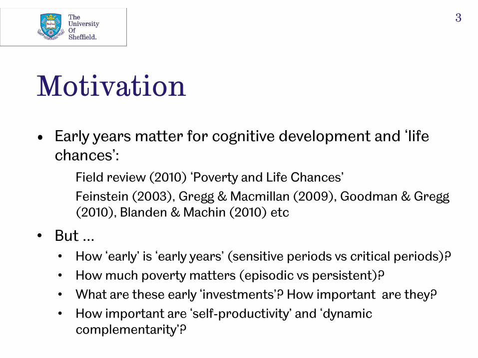
Motivation

• Early years matter for cognitive development and ‘life chances’:

Field review (2010) ‘Poverty and Life Chances’

Feinstein (2003), Gregg & Macmillan (2009), Goodman & Gregg (2010), Blanden & Machin (2010) etc

• But … • How ‘early’ is ‘early years’ (sensitive periods vs critical periods)?

• How much poverty matters (episodic vs persistent)?

• What are these early ‘investments’? How important are they?

• How important are ‘self-productivity’ and ‘dynamic complementarity’?

3

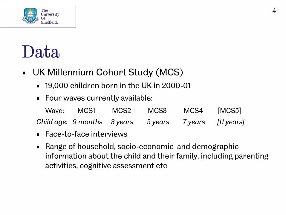
Data • UK Millennium Cohort Study (MCS)

• 19,000 children born in the UK in 2000-01

• Four waves currently available:

Wave: MCS1 MCS2 MCS3 MCS4 [MCS5]

Child age: 9 months 3 years 5 years 7 years [11 years]

• Face-to-face interviews

• Range of household, socio-economic and demographic information about the child and their family, including parenting activities, cognitive assessment etc

4

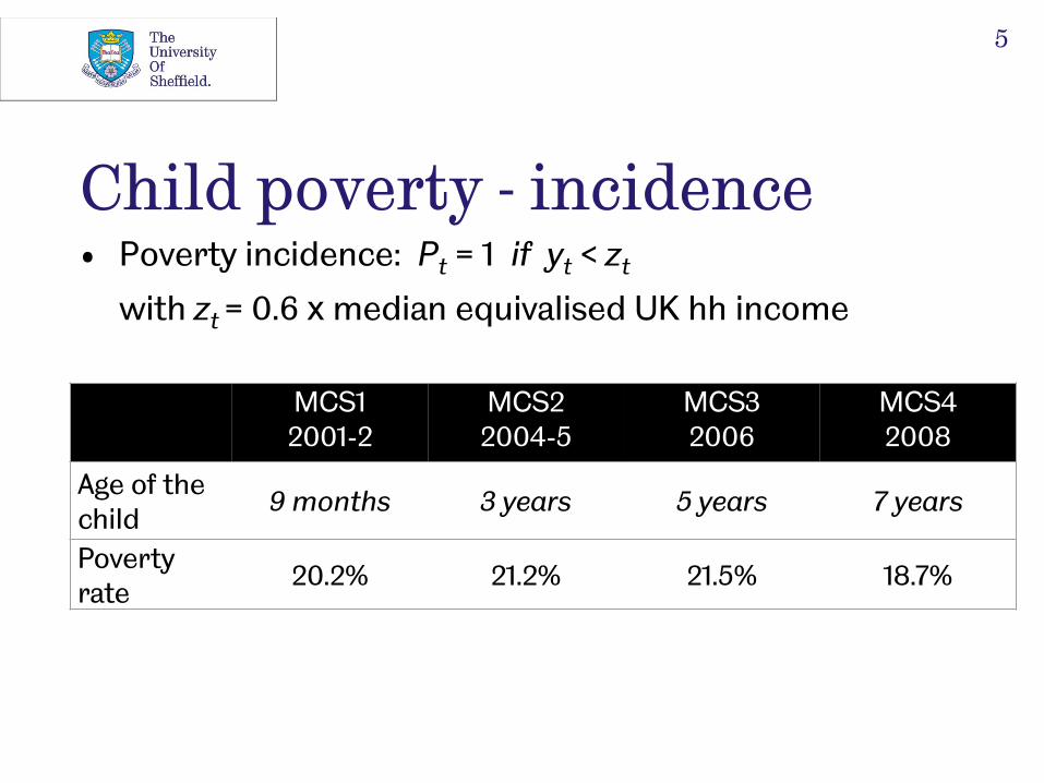
Child poverty - incidence • Poverty incidence: Pt = 1 if yt < zt

with zt = 0.6 x median equivalised UK hh income

5

MCS1 2001-2

MCS2 2004-5

MCS3 2006

MCS4 2008

Age of the child

9 months 3 years 5 years 7 years

Poverty rate

20.2% 21.2% 21.5% 18.7%

Persistent poverty

Time horizon T = 2

Time horizon T = 3

Time horizon T = 4

PS % PS % PS % 00 72.1 000 67.0 0000 64.1 01 7.7 001 5.1 0001 2.9 10 6.7 010 4.1 0010 3.5 11 13.5 100 4.4 0100 3.4

101 2.3 … … 011 3.6 … … 110 2.9 … … 111 10.5 … …

… …

1110 2.4

1111 8.2

6

• Number of poverty states (PS) at wave T is 2T

Cognitive development

• Age-appropriate standardised tests:

MCS2: BAS Naming Vocabulary test (BAS-NV) Bracken School Readiness Assessment (BSRA)

MCS3: BAS Naming Vocabulary test (BAS-NV)

BAS Picture Similarity test (BAS-PS)

BAS Pattern Construction test (BAS-PC)

MCS4: BAS Pattern Construction test (BAS-PC)

BAS Word Reading test (BAS-WR)

Progress in Maths (PiM)

• Compute percentile rankings for each test

7

Child poverty and cognitive development

8

6160

54

61

5758

56 57

32

37

43

36

41

37

4039

0

10

20

30

40

50

60

70

BSRA(3) BAS-NV(3) BAS-PS(5) BAS-NV(5) BAS-PC(5) BAS-WR(7) BAS-PC(7) PiM(7)

Avera

ge r

ank

never in poverty always in poverty

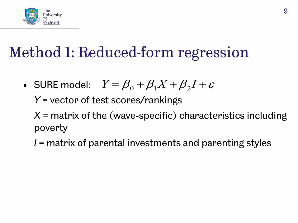
Method 1: Reduced-form regression

• SURE model:

Y = vector of test scores/rankings

X = matrix of the (wave-specific) characteristics including poverty

I = matrix of parental investments and parenting styles

9

IXY 210

Method 1: Reduced-form regression

• One weakness with SURE (and other reduced-form regression-based approaches) is impact of measurement error in cognitive ability (and in parental investment):

• we observe test scores which are correlated with the latent cognitive ability but measure it with error

• leads to problems econometrically and in interpretation (Cunha and Heckman, 2008)

• Also cannot take account of prior cognitive development and/or parental investment – no dynamics

• age-specific tests cannot be compared: Y = f(Y-1 ) is not allowed

10

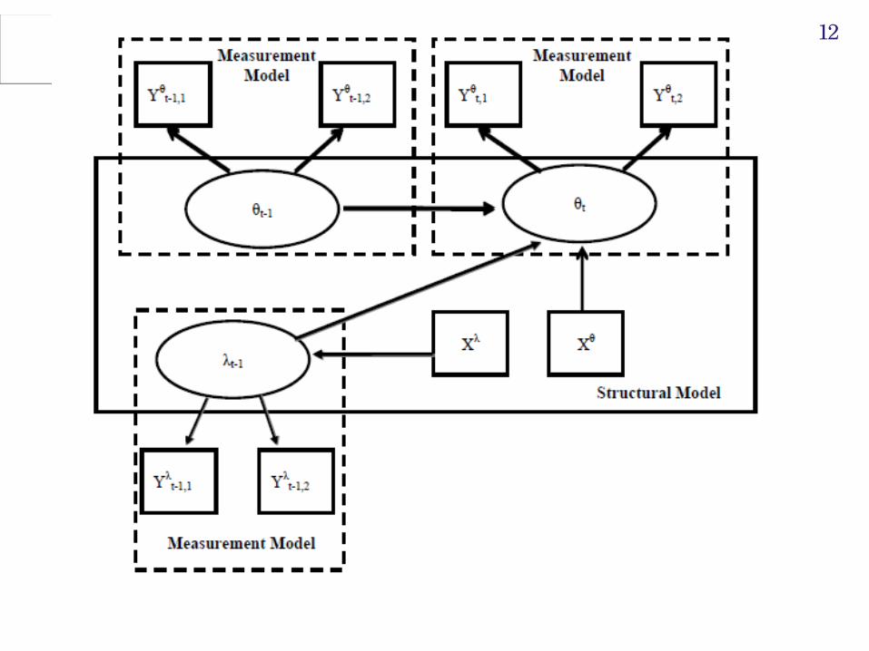
Method 2: Structural Equation Modelling

= latent cognitive skill at time t

= latent parental investment at time t

= matrix of the (wave-specific) characteristics including measure of poverty

Also have initial conditions for t = 1

11

tttttttt BXBA 1211

ttt XB 3

t

t

tX

12

Other advantages of SEM:

1. It allows us to introduce dynamics in the model

while the past latent cognitive ability can reasonably be assumed to influence current latent cognitive ability, the same cannot be said about the test scores

2. It also allows us to capture both the direct and the indirect effect of poverty on cognitive development

Direct effects are simply how poverty affects cognitive development

Indirect effects capture how poverty affects lagged cognitive development, parental investment and parenting style, which in turn impact upon current cognitive development

3. It allows us to utilise ‘incomplete’ observations

13

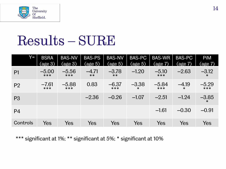
*** significant at 1%; ** significant at 5%; * significant at 10%

Results – SURE

14

Y= BSRA (age 3)

BAS-NV (age 3)

BAS-PS (age 5)

BAS-NV (age 5)

BAS-PC (age 5)

BAS-WR (age 7)

BAS-PC (age 7)

PiM (age 7)

P1 –5.00 ***

–5.56 ***

–4.71 **

–3.78 **

–1.20

–5.10 ***

–2.63

–3.12 *

P2 –7.61 ***

–5.88 ***

0.83

–6.37 ***

–3.38 *

–5.84 ***

–4.19 *

–5.29 ***

P3 –2.36

–0.26

–1.07

–2.51

–1.24

–3.85 *

P4 –1.61

–0.30

–0.91

Controls Yes Yes Yes Yes Yes Yes Yes Yes

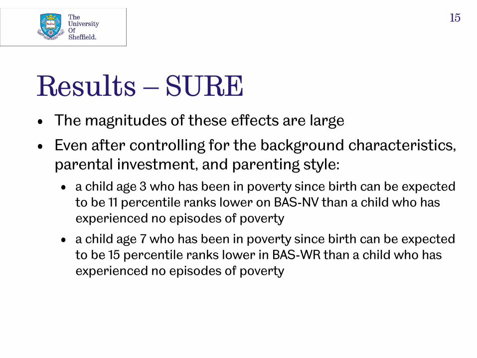
Results – SURE • The magnitudes of these effects are large

• Even after controlling for the background characteristics, parental investment, and parenting style:

• a child age 3 who has been in poverty since birth can be expected to be 11 percentile ranks lower on BAS-NV than a child who has experienced no episodes of poverty

• a child age 7 who has been in poverty since birth can be expected to be 15 percentile ranks lower in BAS-WR than a child who has experienced no episodes of poverty

15

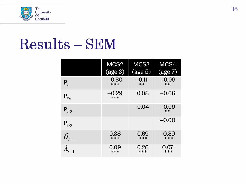
Results – SEM

MCS2 (age 3)

MCS3 (age 5)

MCS4 (age 7)

Pt –0.30

*** –0.11

** -0.09

**

Pt-1 –0.29

*** 0.08

–0.06

Pt-2 –0.04

–0.09

**

Pt-3 –0.00

0.38 ***

0.69 ***

0.89 ***

0.09 ***

0.28 ***

0.07 ***

16

1t

1t

Results – SEM

• Poverty dummies are not that significant after wave 2

i.e. direct effects of poverty on cognitive development are mainly insignificant

• However, indirect effects through lagged latent cognitive ability and latent parental investment are negative and strongly significant

17

Conclusions

• Children born into poverty have significantly lower test scores at age 3, 5 and 7

• Continually living in poverty in early years has a cumulative negative impact on cognitive development, even having controlled for a wide range of background characteristics and parental investment

• Much of the impact of poverty on cognitive development is through its effect on lagged cognitive development and on parental investment

18

Implications

• Emphasis needs to be on early years intervention (birth to age 3) in preventing poverty

since the ‘legacy’ effect of early poverty on cognitive development is so strong

• Good parenting (and ‘life chances’) are necessary but not sufficient for good cognitive development since impact of parental investment significantly reduced if in poverty

19