Chapter 2: The Derivation of Maxwell Equations and the form of the boundary value problem In modern time, physics, including geophysics, solves real-world problems by applying first principles of physics with a much higher capability than merely the analytical solutions for simple, classic problems. This is done with great assistance of sophisticated laboratory experiments and powerful computer techniques, including both the hardware and the software. Nevertheless, all mathematical analysis still deeply roots with fundamental mathematical physics. The mathematical physical principles to rule the electromagnetic problems are the Maxwell equations. James Clerk Maxwell (1831-1879, Figure 2.1) elegantly integrated the electric, magnetic, and the electro-magnetic induction theories prior to his era and formed a set of differential equations. This integration has been known as the Maxwell equations thereafter.

Figure 2.1. James Clerk Maxwell (1831-1879).

The next subsection gives the major derivation of the Maxwell equations. They integrated the Ampere’s law, the Faraday’s law and two mathematical-physical theorems and formed a set of four partial differential equations.

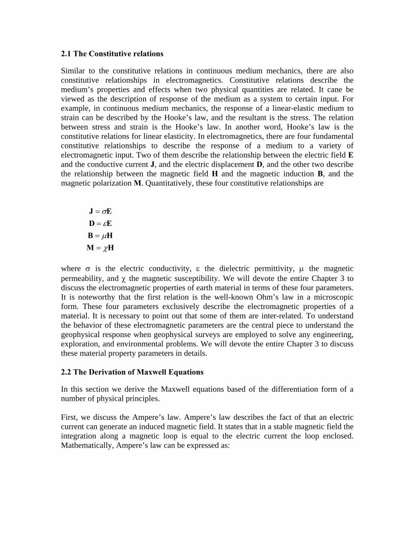
2.1 The Constitutive relations Similar to the constitutive relations in continuous medium mechanics, there are also constitutive relationships in electromagnetics. Constitutive relations describe the medium’s properties and effects when two physical quantities are related. It cane be viewed as the description of response of the medium as a system to certain input. For example, in continuous medium mechanics, the response of a linear-elastic medium to strain can be described by the Hooke’s law, and the resultant is the stress. The relation between stress and strain is the Hooke’s law. In another word, Hooke’s law is the constitutive relations for linear elasticity. In electromagnetics, there are four fundamental constitutive relationships to describe the response of a medium to a variety of electromagnetic input. Two of them describe the relationship between the electric field E and the conductive current J, and the electric displacement D, and the other two describe the relationship between the magnetic field H and the magnetic induction B, and the magnetic polarization M. Quantitatively, these four constitutive relationships are

HMHBEDEJ

χµεσ

====

where σ is the electric conductivity, ε the dielectric permittivity, µ the magnetic permeability, and χ the magnetic susceptibility. We will devote the entire Chapter 3 to discuss the electromagnetic properties of earth material in terms of these four parameters. It is noteworthy that the first relation is the well-known Ohm’s law in a microscopic form. These four parameters exclusively describe the electromagnetic properties of a material. It is necessary to point out that some of them are inter-related. To understand the behavior of these electromagnetic parameters are the central piece to understand the geophysical response when geophysical surveys are employed to solve any engineering, exploration, and environmental problems. We will devote the entire Chapter 3 to discuss these material property parameters in details. 2.2 The Derivation of Maxwell Equations In this section we derive the Maxwell equations based of the differentiation form of a number of physical principles. First, we discuss the Ampere’s law. Ampere’s law describes the fact of that an electric current can generate an induced magnetic field. It states that in a stable magnetic field the integration along a magnetic loop is equal to the electric current the loop enclosed. Mathematically, Ampere’s law can be expressed as:

jdL

=⋅∫ lH

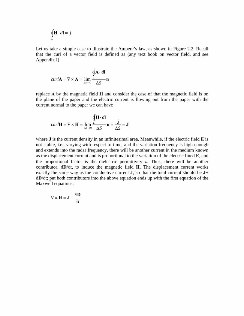
Let us take a simple case to illustrate the Ampere’s law, as shown in Figure 2.2. Recall that the curl of a vector field is defined as (any text book on vector field, and see Appendix I)

nlA

AAS

dcurl L

S ∆

⋅=×∇=

∫→∆ 0

lim

replace A by the magnetic field H and consider the case of that the magnetic field is on the plane of the paper and the electric current is flowing out from the paper with the current normal to the paper we can have

JjnlH

HH =∆

=∆

⋅=×∇=

∫→∆ SS

dcurl L

S 0lim

where J is the current density in an infinitesimal area. Meanwhile, if the electric field E is not stable, i.e., varying with respect to time, and the variation frequency is high enough and extends into the radar frequency, there will be another current in the medium known as the displacement current and is proportional to the variation of the electric fined E, and the proportional factor is the dielectric permittivity ε. Thus, there will be another contributor, dD/dt, to induce the magnetic field H. The displacement current works exactly the same way as the conductive current J, so that the total current should be J+ dD/dt; put both contributors into the above equation ends up with the first equation of the Maxwell equations:

t∂

∂+=×∇

DJH

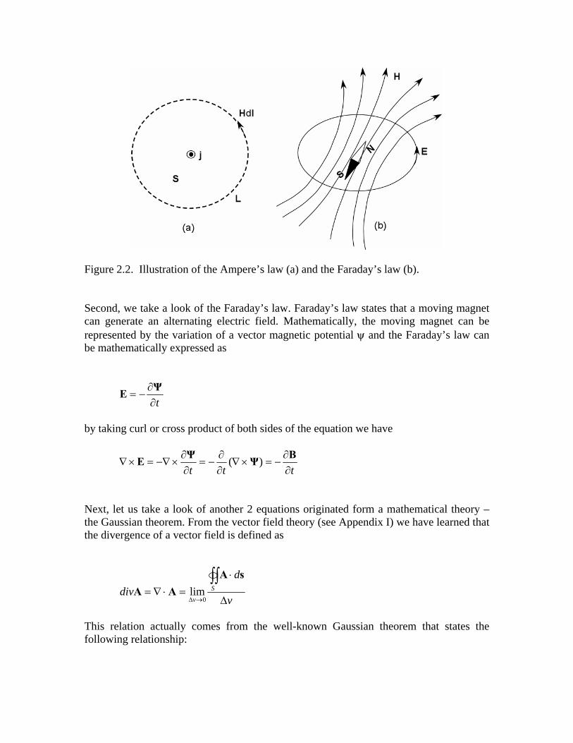
Figure 2.2. Illustration of the Ampere’s law (a) and the Faraday’s law (b). Second, we take a look of the Faraday’s law. Faraday’s law states that a moving magnet can generate an alternating electric field. Mathematically, the moving magnet can be represented by the variation of a vector magnetic potential ψ and the Faraday’s law can be mathematically expressed as

t∂∂

−=ΨE

by taking curl or cross product of both sides of the equation we have

ttt ∂∂

−=×∇∂∂

−=∂∂

×−∇=×∇BΨΨE )(

Next, let us take a look of another 2 equations originated form a mathematical theory – the Gaussian theorem. From the vector field theory (see Appendix I) we have learned that the divergence of a vector field is defined as

v

ddiv S

v ∆

⋅=⋅∇=

∫∫→∆

sAAA

0lim

This relation actually comes from the well-known Gaussian theorem that states the following relationship:

∫∫∫∫∫ ⋅=⋅∇Sv

ddv sAA

Gaussian theorem states that the integration of the divergence of a vector field over a certain volume is equivalent to the vector field itself integrated over the entire closed surface that contains the volume. Applying the divergence and Gaussian theorem to the electric field E and the magnetic field H results in different results. Let’s take a look of the electric field first. From the constitutive relationships we knew that D=εE, and we also knew the electric field caused by an electric charge q is

34 rqπε

rE =

Replacing A with D in the definition of divergence and considering the Gaussian theorem and take the closed surface as a spherical shell centered at the location of the electric charge we have

eS

0v

S

0v

S

0v vq

v

dr

q

v

d

v

d

limlimlim ρπε

εε===

⋅=

⋅=⋅∇

∫∫∫∫∫∫→→→

srsEsDD

34

where ρe is the charge density in the infinitesimal volume confined by the enclosed surface. In contrast, the magnetic field is a completely another story with the fact that the magnetic field is a rotation field with only the dipole source at a singular location and the south and north poles are only separated by a infinitesimal distance. Even when the enclosed surface contains the magnetic source, the net magnetic charge, in analog with the electric field, is still zero. Thus, when apply the divergence and Gaussian theorem to the magnetic induction B we have

0=⋅

=⋅

=⋅∇∫∫∫∫

→→ v

d

v

dS

0v

S

0vlimlim

sHsBB

µ

upon the fact that the net magnetic flux goes through the closed surface is zero (Figure 2.3).

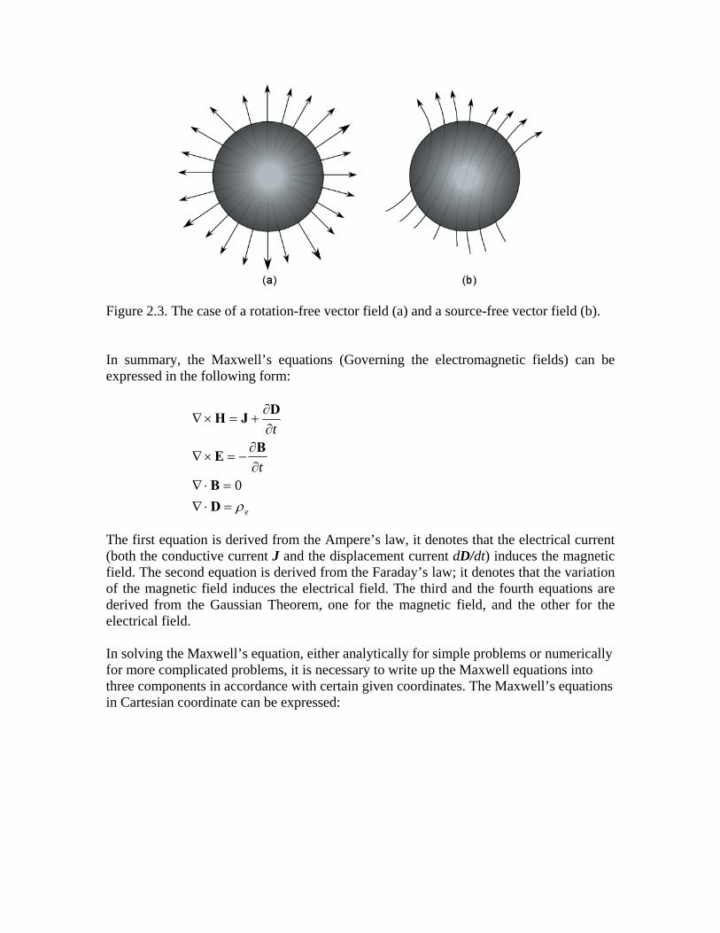
Figure 2.3. The case of a rotation-free vector field (a) and a source-free vector field (b). In summary, the Maxwell’s equations (Governing the electromagnetic fields) can be expressed in the following form:

e

t

t

ρ=⋅∇=⋅∇

∂∂

−=×∇

∂∂

+=×∇

DB

BE

DJH

0

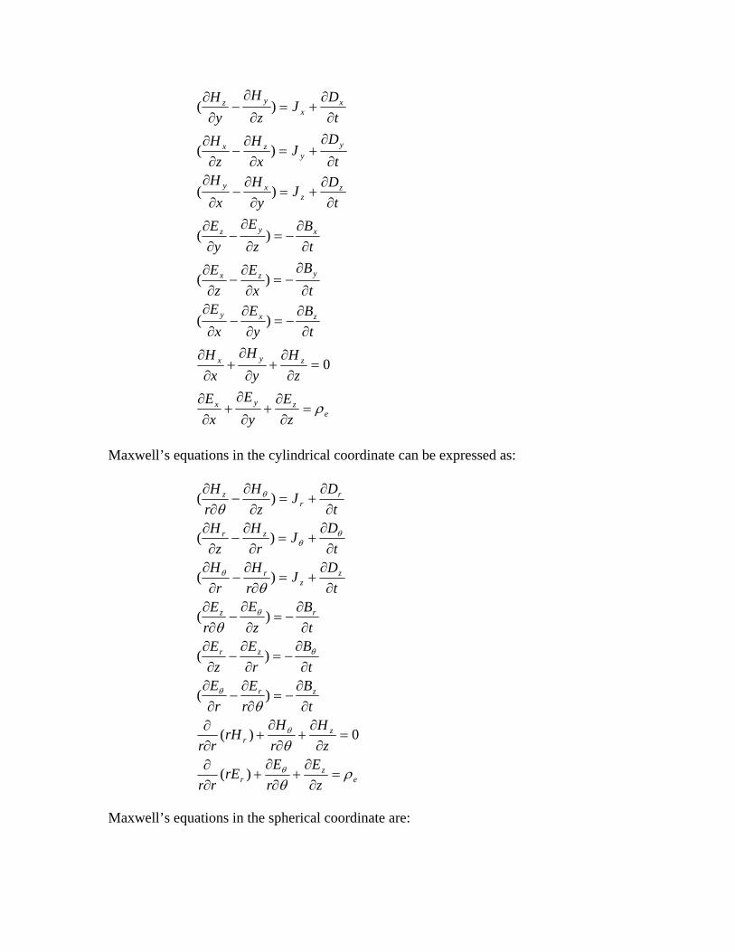
The first equation is derived from the Ampere’s law, it denotes that the electrical current (both the conductive current J and the displacement current dD/dt) induces the magnetic field. The second equation is derived from the Faraday’s law; it denotes that the variation of the magnetic field induces the electrical field. The third and the fourth equations are derived from the Gaussian Theorem, one for the magnetic field, and the other for the electrical field. In solving the Maxwell’s equation, either analytically for simple problems or numerically for more complicated problems, it is necessary to write up the Maxwell equations into three components in accordance with certain given coordinates. The Maxwell’s equations in Cartesian coordinate can be expressed:

ezyx

zyx

zxy

yzx

xyz

zz

xy

yy

zx

xx

yz

zE

yE

xE

zH

yH

xH

tB

yE

xE

tB

xE

zE

tB

zE

yE

tDJ

yH

xH

tD

Jx

Hz

Ht

DJ

zH

yH

ρ=∂

∂+

∂

∂+

∂∂

=∂

∂+

∂

∂+

∂∂

∂∂

−=∂

∂−

∂

∂∂

∂−=

∂∂

−∂

∂

∂∂

−=∂

∂−

∂∂

∂∂

+=∂

∂−

∂

∂∂

∂+=

∂∂

−∂

∂

∂∂

+=∂

∂−

∂∂

0

)(

)(

)(

)(

)(

)(

Maxwell’s equations in the cylindrical coordinate can be expressed as:

ez

r

zr

zr

zr

rz

zz

r

zr

rr

z

zE

rE

rErr

zH

rH

rHrr

tB

rE

rE

tB

rE

zE

tB

zE

rE

tD

JrH

rH

tD

Jr

Hz

Ht

DJ

zH

rH

ρθ

θ

θ

θ

θ

θ

θ

θ

θ

θ

θ

θ

θθ

θ

=∂

∂+

∂∂

+∂∂

=∂

∂+

∂∂

+∂∂

∂∂

−=∂

∂−

∂∂

∂∂

−=∂

∂−

∂∂

∂∂

−=∂

∂−

∂∂

∂∂

+=∂

∂−

∂∂

∂∂

+=∂

∂−

∂∂

∂∂

+=∂

∂−

∂∂

)(

0)(

)(

)(

)(

)(

)(

)(

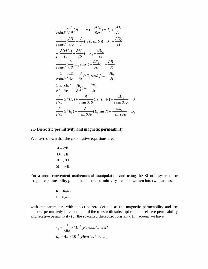
Maxwell’s equations in the spherical coordinate are:

er

r

r

r

r

r

r

rr

rE

Er

Errr

rH

Hr

Hrrr

tBE

rrE

r

tBrE

rE

r

tBEE

r

tD

JHr

rHr

tDJrH

rH

r

tDJHH

r

ρϕθ

θθθ

ϕθθ

θθ

θ

θϕθ

ϕθ

θθ

θ

θϕθ

ϕθ

θθ

ϕθ

ϕθ

ϕθ

θϕ

θϕ

ϕϕ

θ

θθϕ

θϕ

=∂

∂+

∂∂

+∂∂

=∂

∂+

∂∂

+∂∂

∂∂

−=∂∂

−∂

∂

∂∂

−=∂∂

−∂∂

∂∂

−=∂∂

−∂∂

∂∂

+=∂

∂−

∂∂

∂∂

+=∂∂

−∂∂

∂∂

+=∂

∂−

∂∂

sin)sin(

sin)(

0sin

)sin(sin

)(

))((1

))sin((sin1

))sin((sin1

))((1

))sin((sin1

))sin((sin1

22

22

2.3 Dielectric permittivity and magnetic permeability We have shown that the constitutive equations are:

HMHBEDEJ

χµεσ

====

For a more convenient mathematical manipulation and using the SI unit system, the magnetic permeability µ and the electric permittivity ε can be written into two parts as:

r

r

εεεµµµ

0

0

==

with the parameters with subscript zero defined as the magnetic permeability and the electric permittivity in vacuum; and the ones with subscript r as the relative permeability and relative permittivity (or the so-called dielectric constant). In vacuum we have

)/(104

)/(1036

1

70

90

meterHenries

meterFarads

−

−

×=

×=

πµπ

ε

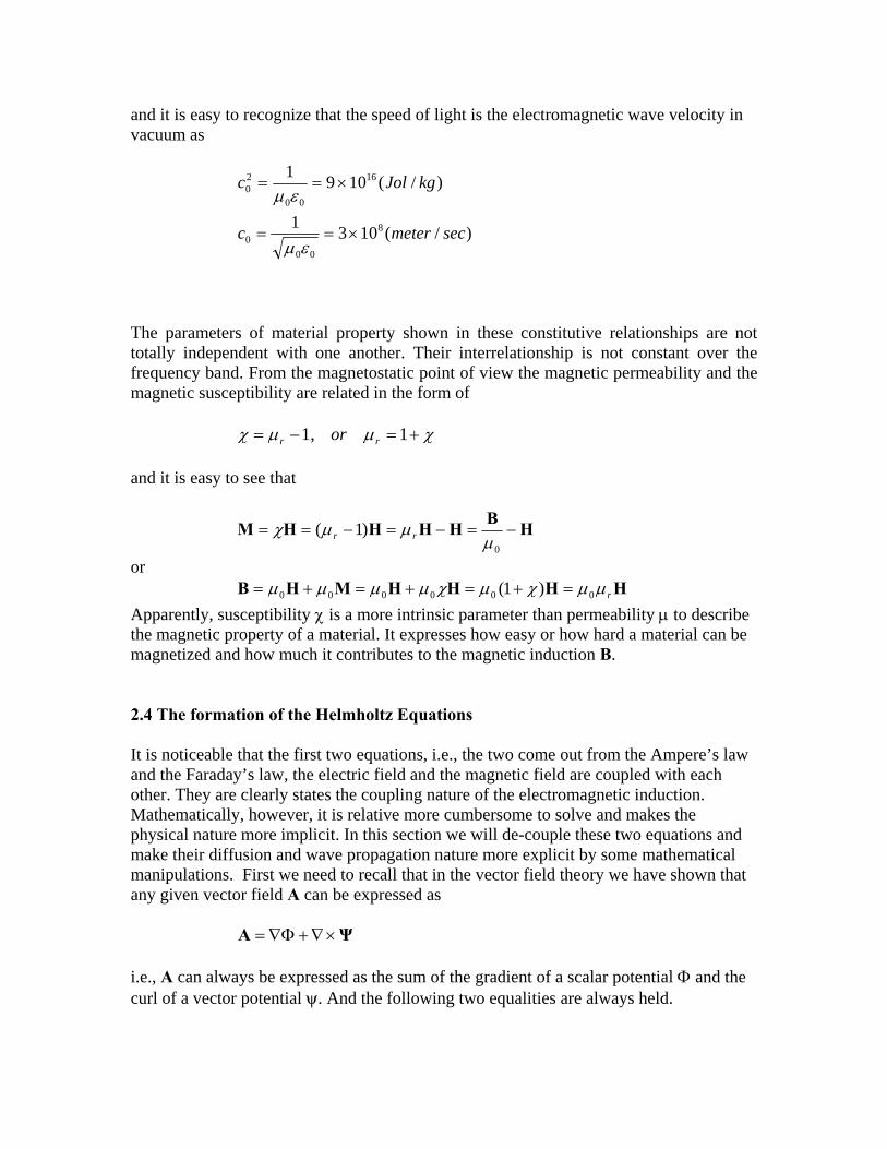
and it is easy to recognize that the speed of light is the electromagnetic wave velocity in vacuum as

)/(1031

)/(1091

8

000

16

00

20

secmeterc

kgJolc

×==

×==

εµ

εµ

The parameters of material property shown in these constitutive relationships are not totally independent with one another. Their interrelationship is not constant over the frequency band. From the magnetostatic point of view the magnetic permeability and the magnetic susceptibility are related in the form of

χµµχ +=−= 1,1 rr or and it is easy to see that

HBHHHHM −=−=−==0

)1(µ

µµχ rr

or HHHHMHB rµµχµχµµµµ 000000 )1( =+=+=+=

Apparently, susceptibility χ is a more intrinsic parameter than permeability µ to describe the magnetic property of a material. It expresses how easy or how hard a material can be magnetized and how much it contributes to the magnetic induction B. 2.4 The formation of the Helmholtz Equations It is noticeable that the first two equations, i.e., the two come out from the Ampere’s law and the Faraday’s law, the electric field and the magnetic field are coupled with each other. They are clearly states the coupling nature of the electromagnetic induction. Mathematically, however, it is relative more cumbersome to solve and makes the physical nature more implicit. In this section we will de-couple these two equations and make their diffusion and wave propagation nature more explicit by some mathematical manipulations. First we need to recall that in the vector field theory we have shown that any given vector field A can be expressed as

ΨA ×∇+Φ∇= i.e., A can always be expressed as the sum of the gradient of a scalar potential Φ and the curl of a vector potential ψ. And the following two equalities are always held.

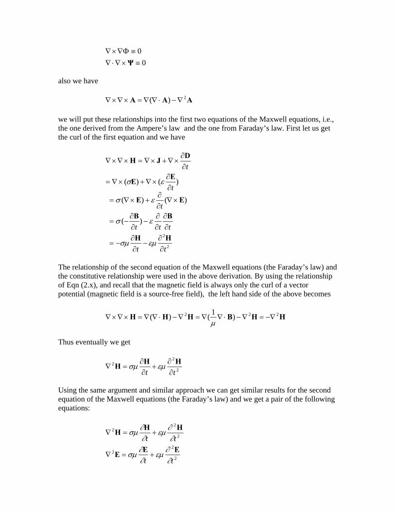
00≡×∇⋅∇

≡Φ∇×∇Ψ

also we have

AAA 2)( ∇−⋅∇∇=×∇×∇ we will put these relationships into the first two equations of the Maxwell equations, i.e., the one derived from the Ampere’s law and the one from Faraday’s law. First let us get the curl of the first equation and we have

2

2

)(

)()(

)()(

tt

ttt

t

t

t

∂∂

−∂∂

−=

∂∂

∂∂

−∂∂

−=

×∇∂∂

+×∇=

∂∂

×∇+×∇=

∂∂

×∇+×∇=×∇×∇

HH

BB

EE

EE

DJH

εµσµ

εσ

εσ

εσ

The relationship of the second equation of the Maxwell equations (the Faraday’s law) and the constitutive relationship were used in the above derivation. By using the relationship of Eqn (2.x), and recall that the magnetic field is always only the curl of a vector potential (magnetic field is a source-free field), the left hand side of the above becomes

HHBHHH 222 )1()( −∇=∇−⋅∇∇=∇−⋅∇∇=×∇×∇µ

Thus eventually we get

2

22

tt ∂∂

+∂∂

=∇HHH εµσµ

Using the same argument and similar approach we can get similar results for the second equation of the Maxwell equations (the Faraday’s law) and we get a pair of the following equations:

2

22

2

22

tt

tt

∂∂εµ

∂∂σµ

∂∂εµ

∂∂σµ

EEE

HHH

+=∇

+=∇

Obviously the two equations have been decoupled, i.e., only one physical quantity (field), either the electric field or the magnetic field, appears in one equation. After decoupling the electric field and the magnetic field we can further the discussion by look into the relativity of the material parameters for the electric and electromagnetic properties. Without lose of generality, we can assume the time variation of the electric field is in a simple harmonic form, i.e.,

EEEEEEEE 202

2

00 ))((,, ωωωωω ωωω −=−−=∂∂

−=−=∂∂

= −−− tititi eiit

ieit

e

Hereinafter we let that E is a newly defined quantity without time varying component and omitted the subscript zero for the easy writing. Put this definition into the second equation of eqn(2.x) we have

E

E

EE

EEE

2

2

2

2

22

)1(

k

i

itt

−=

+−=

−−=

+=∇

ωεσεµω

εµωωσµ∂∂εµ

∂∂σµ

Follow a similar approach we can get the same results for the magnetic field and we thus can arrive at a set of two the so-called Helmholtz equations. The Helmholtz equations

00

22

22

=+∇

=+∇

EEHH

kk

with the definition for

)1(22 ikωεσµεω +=

as the squared complex wave number. It is clear that in the above equation when the second term in the bracket on the right hand side has a value much larger than one then the k-square has a significant imaginary part so that the Helmholtz equation is essentially representing a diffusion equation. Vice versa, if the ratio is much less than one, the k-square has a significant real part so that the Helmholtz equation is essentially representing a wave equation. That is to say, in the complete equations

2

22

2

22

tt

tt

∂∂εµ

∂∂σµ

∂∂εµ

∂∂σµ

EEE

HHH

+=∇

+=∇

if σ>>ωε, we have

t

t

∂∂σµ

∂∂σµ

EE

HH

≈∇

≈∇

2

2

Since most earth materials do not have strong magnetic susceptibility, the electric conductivity is the controlling parameter in the process. Thus the above equation represents a conductive, or diffusion process, similar to the diffusion equation used to describe heat conduction, groundwater flow etc. Mathematically, this is a parabolic equation. On the other hand, if σ<<ωε, we have

2

22

2

22

t

t

∂∂εµ

∂∂εµ

EE

HH

≈∇

≈∇

In this equation the dielectric permittivity is the prevailing parameter (again, magnetic permeability is relative weak for most earth materials). Dielectric polarization is the controlling process other than conduction. The physical feature is the wave propagation like process, similar to the mechanic waves. Mathematically, this is a hyperbolic equation. We will discuss in a more detailed fashion on the diffusion equation in electromagnetic induction, and the wave equation in ground penetrating radar. We also define and discuss in details on the electric conduction and dielectric polarization in material properties in Chapter 3. 2.5 Electromagnetic boundary conditions Electromagnetic shows that the normal component of current, electric displacement, and magnetic induction should be continuous when cross a material interface or boundary; while the tangential component of the electric field and the magnetic field should be continuous cross the material interface. Let us take the magnetic boundary condition as the example to illustrate the calculation. From the Gaussian theorem we have

∫∫∫∫∫ ⋅=⋅∇Sv

ddv sAA

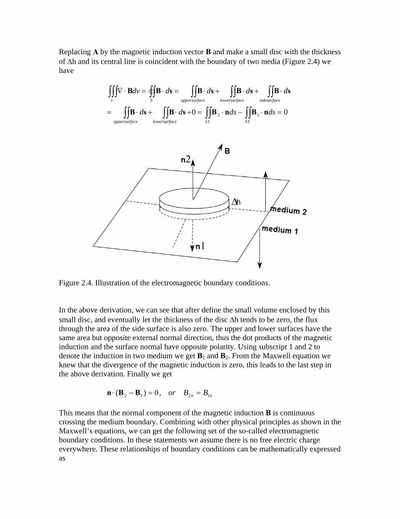
Replacing A by the magnetic induction vector B and make a small disc with the thickness of ∆h and its central line is coincident with the boundary of two media (Figure 2.4) we have

∫∫∫∫∫∫∫∫

∫∫∫∫∫∫∫∫∫∫∫

=⋅−⋅=+⋅+⋅=

⋅+⋅+⋅=⋅=⋅∇

11

12 00

SScelowersurfaceuppersurfa

esidesurfaccelowersurfaceuppersurfaSv

dsdsdd

dddddv

nBnBsBsB

sBsBsBsBB

Figure 2.4. Illustration of the electromagnetic boundary conditions. In the above derivation, we can see that after define the small volume enclosed by this small disc, and eventually let the thickness of the disc ∆h tends to be zero, the flux through the area of the side surface is also zero. The upper and lower surfaces have the same area but opposite external normal direction, thus the dot products of the magnetic induction and the surface normal have opposite polarity. Using subscript 1 and 2 to denote the induction in two medium we get B1 and B2. From the Maxwell equation we knew that the divergence of the magnetic induction is zero, this leads to the last step in the above derivation. Finally we get

nn BBor 1212 ,0)( ==−⋅ BBn This means that the normal component of the magnetic induction B is continuous crossing the medium boundary. Combining with other physical principles as shown in the Maxwell’s equations, we can get the following set of the so-called electromagnetic boundary conditions. In these statements we assume there is no free electric charge everywhere. These relationships of boundary conditions can be mathematically expressed as

0)(0)(0)(0)(0)(

12

12

12

12

12

=−×=−×=−⋅=−⋅=−⋅

EEnHHnDDnBBnJJn

After we discussed the physical equations (the Maxwell’s equations), the constitutive relationships, and the boundary conditions, we are ready to discuss the electromagnetic phenomena in the earth materials. Attenuation: The unit of attenuation coefficient is in Nepers for science and decibels (dB) for engineering. The definitions are

(Np), )xxln(

2

1=α and (dB), )xx(20log

2

110=α

so that the conversion is

.686dB8 (e)dBlog 20dB)

xx

ln(

(e))logxx

ln( 20dB

)xx

ln(

)(e20log dB

)xx

ln(

)xx

(20log Np 1 10

2

1

102

1

2

1

)xx

ln(

10

2

1

2

110 2

1

=====

The following equalities are used in deriving the above relation.

,eln lnx== xex and ,log

1logb

aa

b = if a>0, and b>0

4342945.0ln(10)

1)(log 10 ==e

In summary, neper (Np) is a unit used to express ratios, such as gain, loss, and relative values, here is the attenuation coefficient. The neper is analogous to the decibel, except that the Naperian base e=2.718281828 is used in computing the ratio in nepers. One neper (Np) = 8.686 dB, where 8.686 = 20log(e)=20/(ln 10). The neper is often used to express the ratio of amplitude, whereas the decibel is usually used to express power ratios. Like the dB, the Np is a dimensionless unit.