Embed Size (px)
Citation preview
Technical Report Documentation Page 1. Report No. FHWA/TX-06/0-4822-1
2. Government Accession No.
3. Recipient's Catalog No.
4. Title and Subtitle PERPETUAL PAVEMENTS IN TEXAS: STATE OF THE PRACTICE
5. Report Date May 2006 Published:August 2006
6. Performing Organization Code
7. Author(s) Tom Scullion
8. Performing Organization Report No. Report 0-4822-1 10. Work Unit No. (TRAIS)
9. Performing Organization Name and Address Texas Transportation Institute The Texas A&M University System College Station, Texas 77843-3135
11. Contract or Grant No. Project 0-4822 13. Type of Report and Period Covered Technical Report: September 2004-August 2005
12. Sponsoring Agency Name and Address Texas Department of Transportation Research and Technology Implementation Office P. O. Box 5080 Austin, Texas 78763-5080
14. Sponsoring Agency Code
15. Supplementary Notes Project performed in cooperation with the Texas Department of Transportation and the Federal Highway Administration. Project Title: Monitor Field Performance of Full-Depth Asphalt Pavements to Validate Design Procedures URL: http://tti.tamu.edu/documents/0-4822-1.pdf 16. Abstract As of December 2005 TxDOT has four perpetual pavement sections in service and another four under construction. Project 0-4822 was initiated to perform a structural assessment of these thick asphalt pavements, to identify strengths and weaknesses in the existing structures, and to provide guidance for future designs. This Year 1 report provides an evaluation of the existing sections. It is based on extensive nondestructive testing with Ground Penetrating Radar (GPR), Falling Weight Deflectometers (FWD), field coring, and limited laboratory testing. On a positive note, the stone-filled mixes used in these structures are considerably stiffer than the dense graded mixes traditionally used in Texas. Design moduli values of 750 ksi and 1000 ksi are recommended for future designs with the Stone Matrix Asphalt (SMA) and 1-inch stone-filled (SF) layers. However, three major problems were identified. Firstly, the 1-inch stone-filled layers are prone to vertical segregation. Several of the sections were found to have severe honeycombing at the bottom of the lifts. These mixes are excessively coarse with low asphalt binder contents around 4 percent. Mix design procedures must be modified to eliminate this problem. Secondly, all but one of the projects was found to have de-bonding occurring between layers. This will severely impact the fatigue life of these pavement sections. Thirdly, better guidelines need to be developed on what constitutes a foundation layer for perpetual pavements. Several of the current foundation layers are not thought to be permanent. 17. Key Words Perpetual Pavements, Full-Depth Asphalt Pavements, Non-Destructive Testing, Segregation, Compaction Problems, Stone-Filled Mixes, GPR, FWD
18. Distribution Statement No restrictions. This document is available to the public through NTIS: National Technical Information Service Springfield, Virginia 22161 http://www.ntis.gov
19. Security Classif.(of this report) Unclassified
20. Security Classif.(of this page) Unclassified
21. No. of Pages 90
22. Price
Form DOT F 1700.7 (8-72) Reproduction of completed page authorized

PERPETUAL PAVEMENTS IN TEXAS: STATE OF THE PRACTICE
by
Tom Scullion, P.E. Research Engineer
Texas Transportation Institute
Report 0-4822-1 Project 0-4822
Project Title: Monitor Field Performance of Full-Depth Asphalt Pavements to Validate Design Procedures
Performed in cooperation with the Texas Department of Transportation
and the Federal Highway Administration
May 2006 Published: August 2006
TEXAS TRANSPORTATION INSTITUTE The Texas A&M University System College Station, Texas 77843-3135

v
DISCLAIMER
The contents of this report reflect the views of the author, who is responsible for the facts
and the accuracy of the data presented herein. The contents do not necessarily reflect the official
views or policies of the Texas Department of Transportation or the Federal Highway
Administration. The United States Government and the State of Texas do not endorse products
or manufacturers. Trade or manufacturers’ names appear herein solely because they are
considered essential to the object of this report. This report does not constitute a standard,
specification, or regulation. The engineer in charge was Tom Scullion, P.E. (Texas, # 62683).
vi
ACKNOWLEDGMENTS
This project was made possible by the Texas Department of Transportation and the
Federal Highway Administration. Special thanks must be extended to Joe Leidy, P.E., for
serving as the project director and Miles Garrison, P.E., for serving as the program coordinator.
The following project advisors also provided valuable input throughout the course of the project:
Billy Pigg, P.E., Waco District; Andrew Wimsatt, P.E., Fort Worth District; and Patrick
Downey, P.E., San Antonio.
The assistance of the Laredo, Fort Worth, San Antonio, and Waco Districts is greatly
appreciated in helping with the field studies. Special thanks to Rene Soto in Laredo for going the
extra-mile to help with this research project.
vii
TABLE OF CONTENTS
Page List of Figures .............................................................................................................................. viii
List of Tables ...................................................................................................................................x
Chapter 1. Introduction ...................................................................................................................1
Chapter 2. Structural Evaluation of Existing Section .....................................................................5
Ground Penetrating Radar Evaluation .................................................................................6
Falling Weight Deflectometer Evaluation .........................................................................29
Observations from Coring..................................................................................................36
Mix Design and Placement Details for 1-Inch Stone-Filled Layers ..................................41
District Efforts to Address the Permeability Issues ...........................................................44
Summary ............................................................................................................................46
Chapter 3. Laboratory Testing ......................................................................................................47
Hamburg Wheel Tracking Test..........................................................................................47
Overlay Tester....................................................................................................................48
The Dynamic Modulus Test Protocol ................................................................................50
The Dynamic Modulus Test Results..................................................................................52
Lab Testing Results on Field Cores from the Texas Perpetual Pavements .......................54
Chapter 4. Conclusions and Recommendations............................................................................59
References......................................................................................................................................63
Appendix: FWD Data ...................................................................................................................65
viii
LIST OF FIGURES Figure Page 1. Texas Typical Full-Depth Asphalt Pavement Structural Sections.......................................1
2. GPR Equipment and Principles of Operation ......................................................................7
3. One Individual GPR Trace from a Thick HMA Pavement..................................................9
4. Color-Coded GPR Traces for a 2500-ft Section of Thick Hot Mix...................................10
5. GPR Data from a Thick Black Base Section on IH 10 near
Wurzbach Drive in San Antonio........................................................................................13
6. GPR Data from a Perpetual Pavement on IH 35 in San Antonio (New Braunfels)...........14
7. GPR Data from a Perpetual Pavement on IH 35 in New Braunfels ..................................15
8. GPR Data from Gilbert Job (CSJ 0018-01-063) in the Laredo District ............................17
9. GPR Data from the First Mile of the Zumwalt 1 Project in the Laredo
District (CSJ-0017-08-067) ...............................................................................................18
10. GPR Data from the Transition Section on the Zumwalt 1 Job ..........................................19
11. GPR Results and Cores from the Zumwalt 2 Job (CSJ 0018-02-049)
in the Laredo District .........................................................................................................20
12. GPR Results and a Core from the IH 35 Job in Waco.......................................................22
13. GPR Data Collected on the Hillsboro Perpetual Pavement during Construction..............23
14. GPR Data Collected on the Hillsboro Perpetual Pavement during Construction;
These Data Were Collected One Day after Heavy Rain....................................................24
15. GPR Results and Cores from the SH 114 Project in Fort Worth.......................................27
16. GPR Data from SH 114 Collected after the Edge Drains Were Installed .........................28
17. Temperature Probe Installation..........................................................................................31
18. Intact Cores from the Gilbert Project in Laredo ................................................................36
19. Debonded Core from the Zumwalt 1 Job in Laredo ..........................................................37
20. Inadequate Tack Coat on a Perpetual Pavement................................................................37
21. Severe Vertical Segregation in SF Layers .........................................................................38
22. Cores Taken from the Perpetual Pavement in Waco .........................................................39
23. Cores Taken from the Zumwalt 2 Project in Laredo (Upper) and Young
Brothers Project in Waco (Lower).....................................................................................40
ix
LIST OF FIGURES (CONTINUED) Figure Page 24. Gradation Curves for the 1-Inch SF Layer ........................................................................42
25. Coarse Texture of the 1-Inch SF Mix Used in San Antonio..............................................42
26. Releasing Trapped Water from the Stone-Filled Asphalt Layers on SH 114....................45
27. Installing Edge Drains in SH 114 to Drain Water Trapped within the SF Layers.............45
28. The Hamburg Test Device .................................................................................................47
29. Overlay Tester....................................................................................................................48
30. UTM-25 and HMAC Specimen Setup...............................................................................51
31. Loading Configuration for the DM Test............................................................................51
32. Sample Preparation Procedures for DM Test ....................................................................57
x
LIST OF TABLES Table Page 1. Existing Perpetual Pavements in Texas (as of December 2005) .........................................2
2. Structural Section, Layer Thickness, and PG Grade of Binder ...........................................5
3. FWD Backcalculated Moduli Values for the 1-Inch SF Layers ........................................33
4. FWD Backcalculated Moduli for SMA/¾-Inch SF Combination .....................................34
5. Gradations for 1-Inch SF Layers........................................................................................41
6. Mix Design and Construction Details for 1-Inch SF Layer...............................................43
7. Hamburg and Overlay Tester Results from Field Cores, Hamburg mm,
(Overlay Tester cycles to Failure)......................................................................................49
8. DM Test Results ................................................................................................................53
9. Dynamic Modulus Test Results for the 1-Inch SF Layers from the Gilbert
and Zumwalt 1 Jobs in Laredo...........................................................................................55
10. Comparison of Lab and Field Moduli for the 1-Inch SF Layer from
the Laredo District .............................................................................................................56
1
CHAPTER 1 INTRODUCTION
On March 29, 2001, a memorandum was sent by TxDOT’s Engineering Director to all
district engineers providing guidance on the design of pavements when more than 30 million
Equivalent Single Axle Loads (ESALs) are exceeded (1). This guidance was developed by the
Flexible Pavement Design Task Force, which consisted of senior TxDOT engineers and
representatives from the Asphalt Institute, Texas Asphalt Pavement Association, and various
industry groups. The objectives of the task force were to develop new asphalt concrete
specifications and pavement designs that could meet the demands of heavy truck traffic. A
suggested typical section was prescribed similar to the perpetual pavement concept developed by
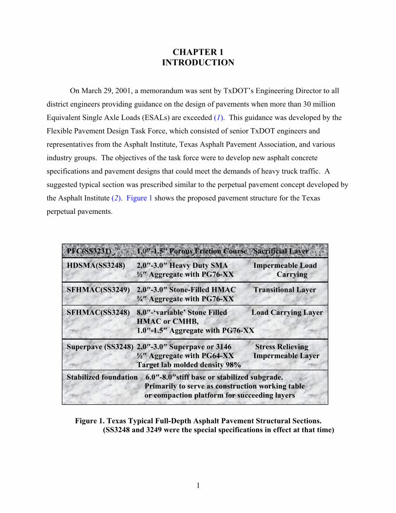
the Asphalt Institute (2). Figure 1 shows the proposed pavement structure for the Texas
perpetual pavements.
Figure 1. Texas Typical Full-Depth Asphalt Pavement Structural Sections. (SS3248 and 3249 were the special specifications in effect at that time)
PFC(SS3231) 1.0″-1.5″ Porous Friction Course Sacrificial Layer
HDSMA(SS3248) 2.0″-3.0″ Heavy Duty SMA Impermeable Load ½″ Aggregate with PG76-XX Carrying
SFHMAC(SS3249) 2.0″-3.0″ Stone-Filled HMAC Transitional Layer ¾″ Aggregate with PG76-XX
SFHMAC(SS3248) 8.0″-‘variable’ Stone Filled Load Carrying Layer HMAC or CMHB,
1.0″-1.5″ Aggregate with PG76-XX
Superpave (SS3248) 2.0″-3.0″ Superpave or 3146 Stress Relieving ½″ Aggregate with PG64-XX Impermeable Layer Target lab molded density 98% Stabilized foundation 6.0″-8.0″stiff base or stabilized subgrade. Primarily to serve as construction working table or compaction platform for succeeding layers
2
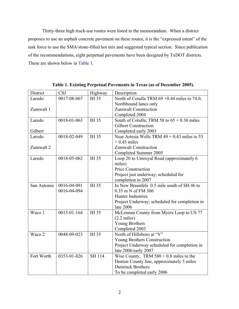
Thirty-three high truck-use routes were listed in the memorandum. When a district
proposes to use an asphalt concrete pavement on these routes, it is the “expressed intent” of the
task force to use the SMA/stone-filled hot mix and suggested typical section. Since publication
of the recommendations, eight perpetual pavements have been designed by TxDOT districts.
These are shown below in Table 1.
Table 1. Existing Perpetual Pavements in Texas (as of December 2005).
District CSJ Highway Description Laredo Zumwalt 1
0017-08-067 IH 35 North of Cotulla TRM 69 +0.44 miles to 74.0, Northbound lanes only Zumwalt Construction Completed 2004
Laredo Gilbert
0018-01-063 IH 35 South of Cotulla; TRM 58 to 65 + 0.36 miles Gilbert Construction Completed early 2003
Laredo Zumwalt 2
0018-02-049 IH 35 Near Artesia Wells TRM 49 + 0.43 miles to 53 + 0.43 miles Zumwalt Construction Completed Summer 2005
Laredo 0018-05-062 IH 35 Loop 20 to Uniroyal Road (approximately 6 miles) Price Construction Project just underway; scheduled for completion in 2007
San Antonio 0016-04-091 0016-04-094
IH 35 In New Braunfels 0.5 mile south of SH 46 to 0.35 m N of FM 306 Hunter Industries Project Underway; scheduled for completion in late 2006
Waco 1 0015-01-164 IH 35 McLennan County from Myers Loop to US 77 (2.2 miles) Young Brothers Completed 2003
Waco 2 0048-09-023 IH 35 North of Hillsboro at “Y” Young Brothers Construction Project Underway scheduled for completion in late 2006/early 2007
Fort Worth 0353-01-026 SH 114 Wise County, TRM 580 + 0.8 miles to the Denton County line, approximately 5 miles Duininck Brothers To be completed early 2006
3
The mix design for these projects followed Special Specification 3248, SS 3249, and
3231, which were developed based largely on national recommendations as proposed by the
Asphalt Institute, incorporating many of the requirements of the Superpave mixture design
system. These special specifications were subsequently revised and incorporated into TxDOT’s
2004 Standard Specifications Book as Porous Friction Courses Item 342 and Performance Mixes
Item 344, and Stone-Matrix Asphalt Item 346.
To date all the mixes used in the Texas Perpetual Pavements were designed using the
Superpave volumetric design system with 100 gyrations to achieve the 4 percent air voids; the
mixes also were required to pass the Hamburg Wheel tracking test. TxDOT has limited field
experience with all of these mixes, in particular the 1-inch and ¾-inch stone-filled (SF) layers
have not previously been placed. These were intended to provide high stiffness and superior rut
resistance.
The goal of Project 0-4822 is to monitor the performance of the existing projects, to test
the materials in the field and laboratory, and to identify the lessons learned for these initial
projects in order to improve future full-depth designs. In particular it is intended to focus on:
• validating the full-depth pavement design concept by relating field and laboratory results
to pavement performance monitored after construction,
• creating a database of design parameters for the current Flexible Pavement System (FPS)
design system and the National Cooperative Highway Research Program (NCHRP) 1-
37A mechanistic design process and the Asphalt Alliance design methodology, and
• using the data collected to verify and enhance TxDOT’s design, materials and
construction specifications.
This is the Year 1 report for Project 0-4822; it consists of the results of a structural
evaluation of the existing sections. The current thickness designs are based on the FPS19
program. A comparison will be given of the assumed design moduli used in the program
compared with those found in the field from Falling Weight Deflectometer (FWD) testing.
Recommendations will be given for a new set of design moduli for future projects.

5
CHAPTER 2
STRUCTURAL EVALUATION OF EXISTING SECTION
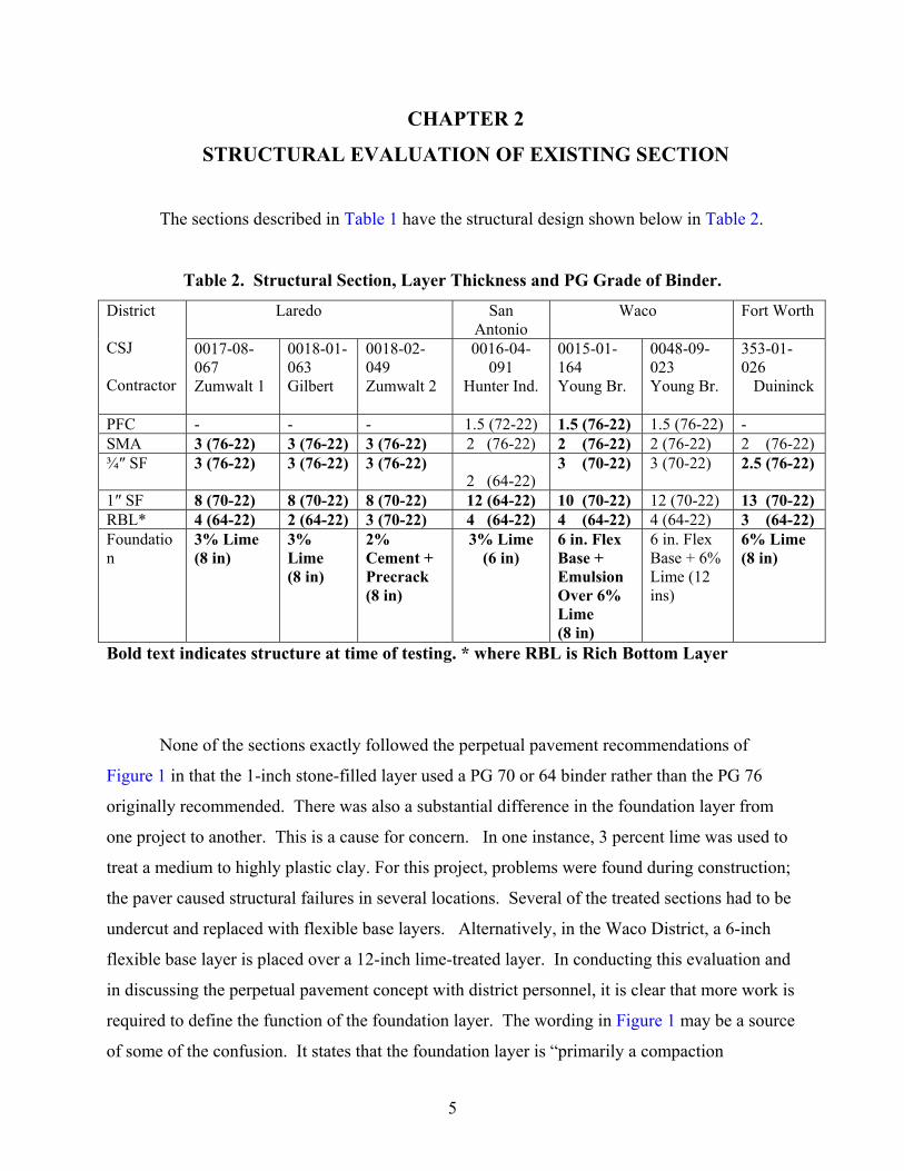
The sections described in Table 1 have the structural design shown below in Table 2.
Table 2. Structural Section, Layer Thickness and PG Grade of Binder.
Laredo San Antonio
Waco Fort Worth District CSJ Contractor
0017-08-067 Zumwalt 1
0018-01-063 Gilbert
0018-02-049 Zumwalt 2
0016-04-091
Hunter Ind.
0015-01-164 Young Br.
0048-09-023 Young Br.
353-01- 026 Duininck
PFC - - - 1.5 (72-22) 1.5 (76-22) 1.5 (76-22) - SMA 3 (76-22) 3 (76-22) 3 (76-22) 2 (76-22) 2 (76-22) 2 (76-22) 2 (76-22) ¾″ SF 3 (76-22) 3 (76-22) 3 (76-22)
2 (64-22) 3 (70-22) 3 (70-22) 2.5 (76-22)
1″ SF 8 (70-22) 8 (70-22) 8 (70-22) 12 (64-22) 10 (70-22) 12 (70-22) 13 (70-22) RBL* 4 (64-22) 2 (64-22) 3 (70-22) 4 (64-22) 4 (64-22) 4 (64-22) 3 (64-22) Foundation
3% Lime (8 in)
3% Lime (8 in)
2% Cement + Precrack (8 in)
3% Lime (6 in)
6 in. Flex Base + Emulsion Over 6% Lime (8 in)
6 in. Flex Base + 6% Lime (12 ins)
6% Lime (8 in)
Bold text indicates structure at time of testing. * where RBL is Rich Bottom Layer
None of the sections exactly followed the perpetual pavement recommendations of
Figure 1 in that the 1-inch stone-filled layer used a PG 70 or 64 binder rather than the PG 76
originally recommended. There was also a substantial difference in the foundation layer from
one project to another. This is a cause for concern. In one instance, 3 percent lime was used to
treat a medium to highly plastic clay. For this project, problems were found during construction;
the paver caused structural failures in several locations. Several of the treated sections had to be
undercut and replaced with flexible base layers. Alternatively, in the Waco District, a 6-inch
flexible base layer is placed over a 12-inch lime-treated layer. In conducting this evaluation and
in discussing the perpetual pavement concept with district personnel, it is clear that more work is
required to define the function of the foundation layer. The wording in Figure 1 may be a source
of some of the confusion. It states that the foundation layer is “primarily a compaction
6
platform.” This concept is not correct. The foundation layer needs to provide permanent support
for the asphalt layers throughout the design life of the pavement. Numerous forensic
investigations in Texas have found that excessive roughness can be found in flexible pavements
if the foundation layer is not permanently stabilized. It is highly doubtful that a 3 percent lime-
treated subgrade will provide an adequate foundation layer. More work is needed in this area.
The main part of this evaluation will focus on the use of TxDOT’s existing
Nondestructive testing (NDT) technologies to structurally evaluate these pavement sections. The
perpetual pavements shown in Table 2 are very thick, and they are not expected to exhibit any
structural damage for a number of years. It is, therefore, very important to use TxDOTs Falling
Weight Deflectometers and Ground Penetrating Radar (GPR) technologies to identify problems
with these structures.
GROUND PENETRATING RADAR EVALUATION
Basics of GPR
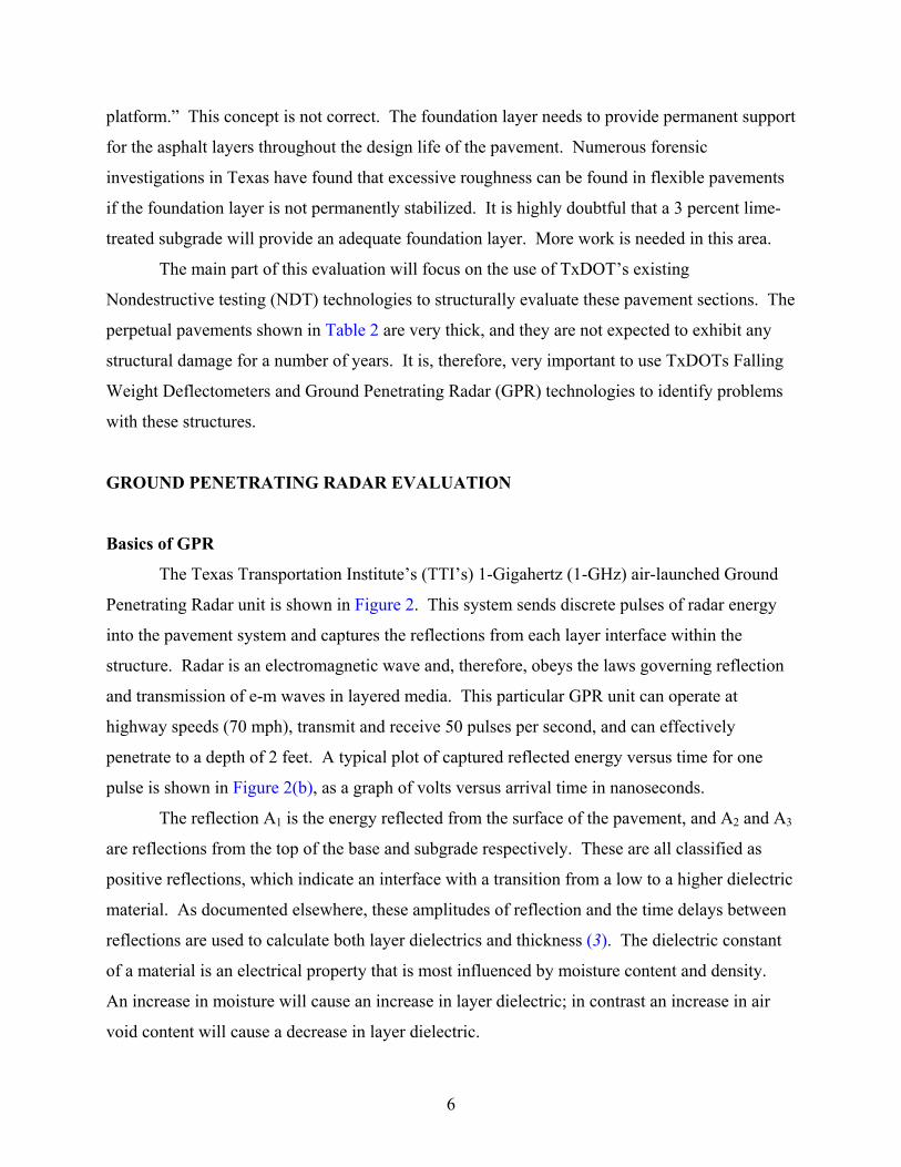
The Texas Transportation Institute’s (TTI’s) 1-Gigahertz (1-GHz) air-launched Ground
Penetrating Radar unit is shown in Figure 2. This system sends discrete pulses of radar energy
into the pavement system and captures the reflections from each layer interface within the
structure. Radar is an electromagnetic wave and, therefore, obeys the laws governing reflection
and transmission of e-m waves in layered media. This particular GPR unit can operate at
highway speeds (70 mph), transmit and receive 50 pulses per second, and can effectively
penetrate to a depth of 2 feet. A typical plot of captured reflected energy versus time for one
pulse is shown in Figure 2(b), as a graph of volts versus arrival time in nanoseconds.
The reflection A1 is the energy reflected from the surface of the pavement, and A2 and A3
are reflections from the top of the base and subgrade respectively. These are all classified as
positive reflections, which indicate an interface with a transition from a low to a higher dielectric
material. As documented elsewhere, these amplitudes of reflection and the time delays between
reflections are used to calculate both layer dielectrics and thickness (3). The dielectric constant
of a material is an electrical property that is most influenced by moisture content and density.
An increase in moisture will cause an increase in layer dielectric; in contrast an increase in air
void content will cause a decrease in layer dielectric.
7
Figure 2. GPR Equipment and Principles of Operation.
8
The examples below illustrate how changes in the pavement’s engineering properties
would influence the typical GPR trace shown in Figure 2b.
• If the thickness of the surface layer increases, then the time interval ∆t1 between
A1 and A2 would increase.
• If the base layer becomes wetter, then the amplitude of reflection from the top of
the base A2 would increase.
• For well-compacted hot mix layers, the GPR wave would be reflected at the top
of the asphalt layer and the top of the base layer. If the asphalt layer has uniform
density with depth, then no intermediate reflections would be observed. If there is
a significant defect within the surface layer, then an additional reflection will be
observed between A1 and A2. This could indicate areas of poor compaction or
moisture trapped between pavement layers. The occurrence of strong reflections
from within/between the asphalt layers of the perpetual pavements will be
described in the remainder of this section.
• Large changes in the surface reflection A1 would indicate changes in either the
density or moisture content along the section. The variation in surface reflection is
used to check segregation within a new HMA surface layer, and it can also be
used to test the quality of longitudinal construction joints.
In most GPR projects, researchers collect several thousand GPR traces. In order to
conveniently display this information, color-coding schemes are used to convert the traces into
line scans and stack them side-by-side so that a subsurface image of the pavement structure can
be obtained. This approach is used extensively in Texas. A typical display from a thick hot mix
asphalt pavement is shown in Figures 3 and 4. This is taken from a section of newly constructed
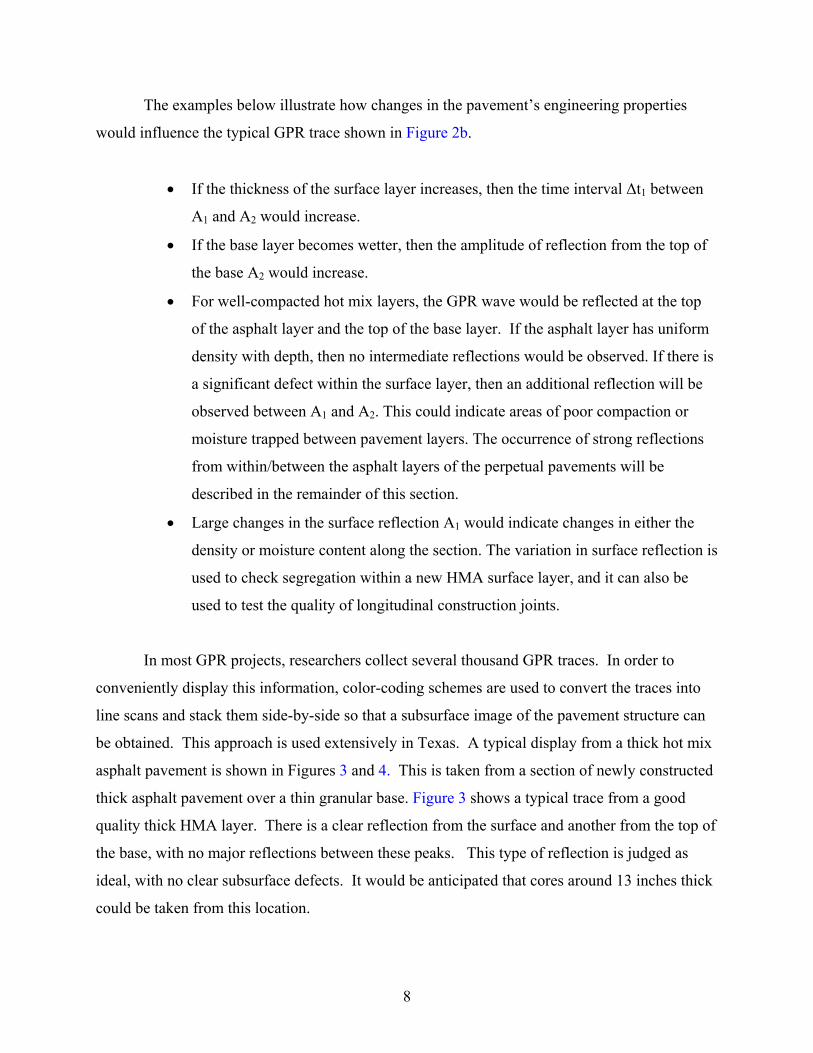
thick asphalt pavement over a thin granular base. Figure 3 shows a typical trace from a good
quality thick HMA layer. There is a clear reflection from the surface and another from the top of
the base, with no major reflections between these peaks. This type of reflection is judged as
ideal, with no clear subsurface defects. It would be anticipated that cores around 13 inches thick
could be taken from this location.
9
Figure 3. One Individual GPR Trace from a Thick HMA Pavement.
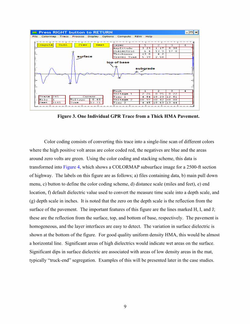
Color coding consists of converting this trace into a single-line scan of different colors
where the high positive volt areas are color coded red, the negatives are blue and the areas
around zero volts are green. Using the color coding and stacking scheme, this data is
transformed into Figure 4, which shows a COLORMAP subsurface image for a 2500-ft section
of highway. The labels on this figure are as follows; a) files containing data, b) main pull down
menu, c) button to define the color coding scheme, d) distance scale (miles and feet), e) end
location, f) default dielectric value used to convert the measure time scale into a depth scale, and
(g) depth scale in inches. It is noted that the zero on the depth scale is the reflection from the
surface of the pavement. The important features of this figure are the lines marked H, I, and J;
these are the reflection from the surface, top, and bottom of base, respectively. The pavement is
homogeneous, and the layer interfaces are easy to detect. The variation in surface dielectric is
shown at the bottom of the figure. For good quality uniform density HMA, this would be almost
a horizontal line. Significant areas of high dielectrics would indicate wet areas on the surface.
Significant dips in surface dielectric are associated with areas of low density areas in the mat,
typically “truck-end” segregation. Examples of this will be presented later in the case studies.
10
Figure 4. Color-Coded GPR Traces for a 2500-ft Section of Thick Hot Mix.
The traces shown in Figures 3 and 4 would be ideal for perpetual pavements. However,
as will be discussed below, the traces obtained from the perpetual pavements constructed in
Texas to date do not show this ideal GPR signature.
GPR Data from TxDOT’s Perpetual Pavements
All of the perpetual pavements in Texas have been tested with GPR, and typical results
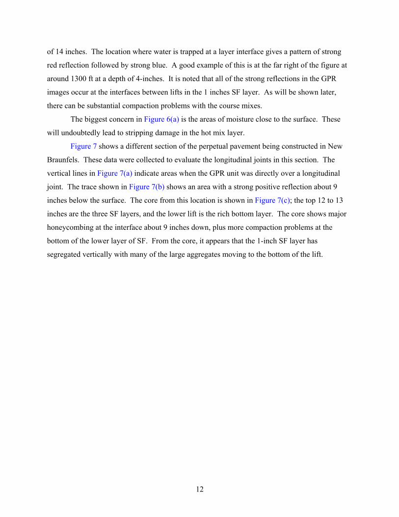
are presented in Figures 6 through 15. Figure 5 from a thick asphalt pavement (not perpetual)
has been included for comparison purposes.
TxDOT has been successfully using thick hot mix sections on heavily trafficked highway
sections for many years. Both the Austin and San Antonio Districts have many miles of very
thick hot mix pavements. Figure 5 shows GPR data from one section in San Antonio from IH
10. This structure was used widely in San Antonio in the 1970s and 1980s. It consists of a thick
densely graded Type A layer (Item 340) followed by various fine-graded surface layers. The
total thickness of the asphalt is close to 24 inches.
The upper figure shows the COLORMAP display for a 1000-ft section of highway. The
lower plot is an individual reflection from one specific location. In the upper figure, the surface
is normalized to the top of the figure. The depth scale is on the left, the only other strong
11
reflection is the reflection about 24 inches down, which is the top of the base layer. No strong
reflections are found between the reflections from the surface and the top of the base. In the
lower figure, the reflections from the surface and top of base are marked with (+). The box in
the upper right shows the computed layer dielectrics and thickness.
From our experience with GPR, these data would indicate a well-compacted mat with
little or no problems at the layer interfaces. It would be expected that solid cores could be taken
from this location. The GPR results from this section should be contrasted with those from
perpetual pavements studied in this project to date.
It is not intended to claim that all the full-depth graded mixes were not subject to
segregation and compaction problems. That is not the case; several forensic studies, such as the
one on US 290 in Houston, have found that segregation can be a problem with these mixes. The
point is that Figure 5 is the ideal target GPR image for thick hot mix pavements, and as will be
described below, has proven difficult to achieve with the current perpetual pavements.
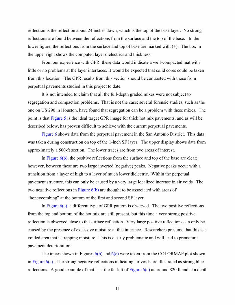
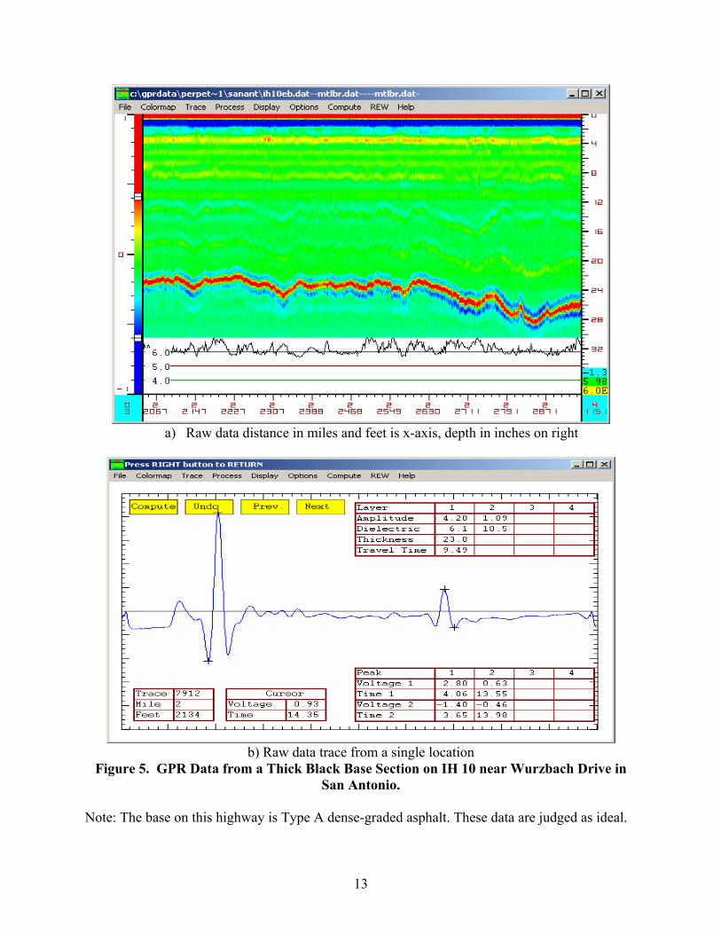
Figure 6 shows data from the perpetual pavement in the San Antonio District. This data
was taken during construction on top of the 1-inch SF layer. The upper display shows data from
approximately a 500-ft section. The lower traces are from two areas of interest.
In Figure 6(b), the positive reflections from the surface and top of the base are clear;
however, between these are two large inverted (negative) peaks. Negative peaks occur with a
transition from a layer of high to a layer of much lower dielectric. Within the perpetual
pavement structure, this can only be caused by a very large localized increase in air voids. The
two negative reflections in Figure 6(b) are thought to be associated with areas of
“honeycombing” at the bottom of the first and second SF layer.
In Figure 6(c), a different type of GPR pattern is observed. The two positive reflections
from the top and bottom of the hot mix are still present, but this time a very strong positive
reflection is observed close to the surface reflection. Very large positive reflections can only be
caused by the presence of excessive moisture at this interface. Researchers presume that this is a
voided area that is trapping moisture. This is clearly problematic and will lead to premature
pavement deterioration.
The traces shown in Figures 6(b) and 6(c) were taken from the COLORMAP plot shown
in Figure 6(a). The strong negative reflections indicating air voids are illustrated as strong blue
reflections. A good example of that is at the far left of Figure 6(a) at around 820 ft and at a depth
12
of 14 inches. The location where water is trapped at a layer interface gives a pattern of strong
red reflection followed by strong blue. A good example of this is at the far right of the figure at
around 1300 ft at a depth of 4-inches. It is noted that all of the strong reflections in the GPR
images occur at the interfaces between lifts in the 1 inches SF layer. As will be shown later,
there can be substantial compaction problems with the course mixes.
The biggest concern in Figure 6(a) is the areas of moisture close to the surface. These
will undoubtedly lead to stripping damage in the hot mix layer.
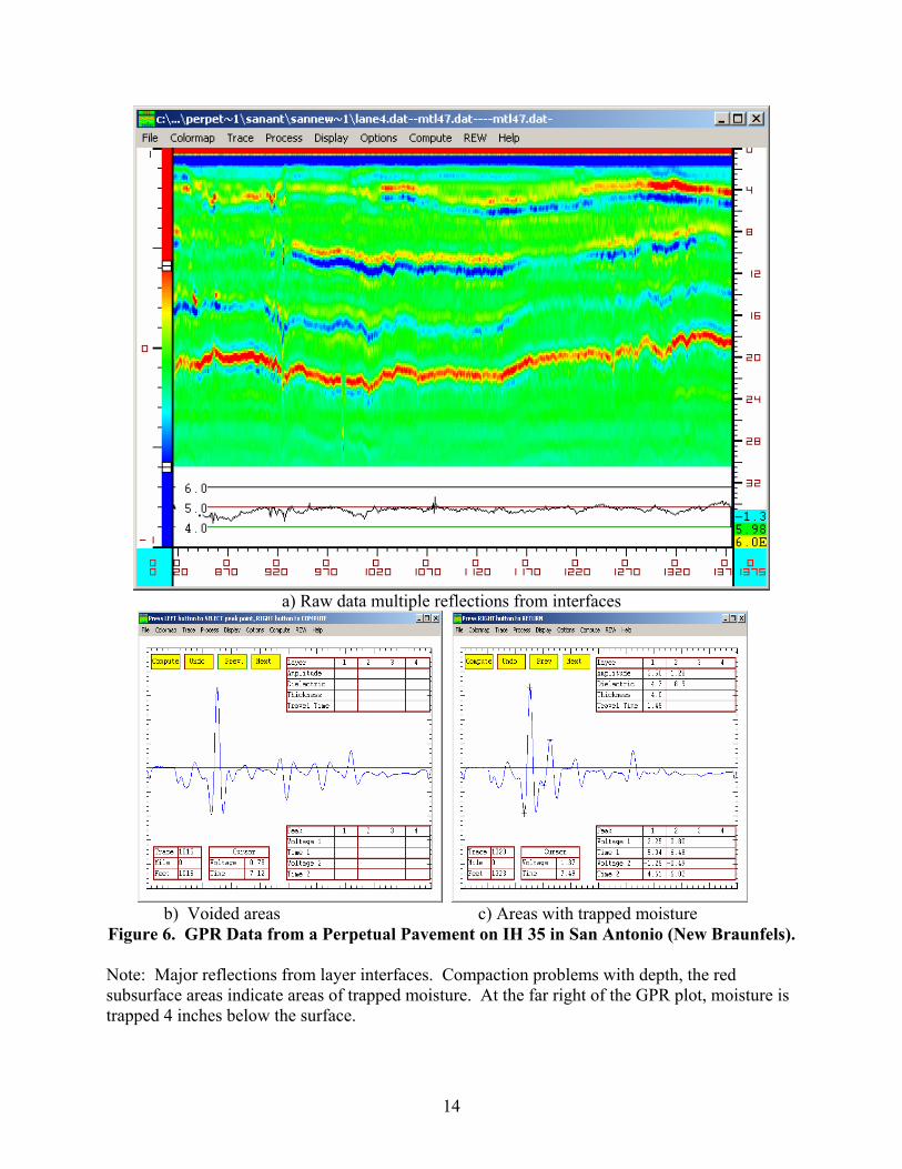
Figure 7 shows a different section of the perpetual pavement being constructed in New
Braunfels. These data were collected to evaluate the longitudinal joints in this section. The
vertical lines in Figure 7(a) indicate areas when the GPR unit was directly over a longitudinal
joint. The trace shown in Figure 7(b) shows an area with a strong positive reflection about 9
inches below the surface. The core from this location is shown in Figure 7(c); the top 12 to 13
inches are the three SF layers, and the lower lift is the rich bottom layer. The core shows major
honeycombing at the interface about 9 inches down, plus more compaction problems at the
bottom of the lower layer of SF. From the core, it appears that the 1-inch SF layer has
segregated vertically with many of the large aggregates moving to the bottom of the lift.
13
a) Raw data distance in miles and feet is x-axis, depth in inches on right
b) Raw data trace from a single location
Figure 5. GPR Data from a Thick Black Base Section on IH 10 near Wurzbach Drive in San Antonio.
Note: The base on this highway is Type A dense-graded asphalt. These data are judged as ideal.
14
a) Raw data multiple reflections from interfaces
b) Voided areas c) Areas with trapped moisture
Figure 6. GPR Data from a Perpetual Pavement on IH 35 in San Antonio (New Braunfels). Note: Major reflections from layer interfaces. Compaction problems with depth, the red subsurface areas indicate areas of trapped moisture. At the far right of the GPR plot, moisture is trapped 4 inches below the surface.
15
a) Blue marks indicate location of longitudinal joints
b) Trapped water c) Resulting core Figure 7. GPR Data from a Perpetual Pavement on IH 35 in New Braunfels.
Note: These data were collected over longitudinal joints. The markers in the upper figure are when the GPR unit passed over a joint. The core was taken close to a longitudinal joint. The red areas in the middle of the layers indicate trapped moisture.
16
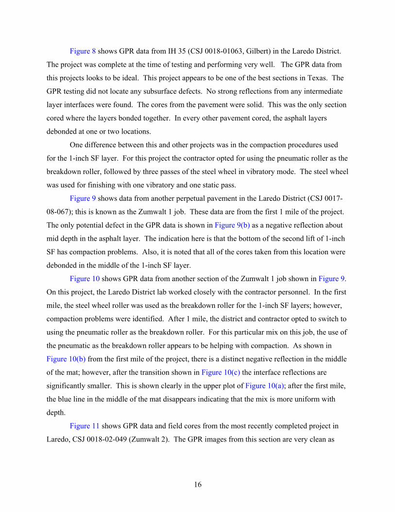
Figure 8 shows GPR data from IH 35 (CSJ 0018-01063, Gilbert) in the Laredo District.
The project was complete at the time of testing and performing very well. The GPR data from
this projects looks to be ideal. This project appears to be one of the best sections in Texas. The
GPR testing did not locate any subsurface defects. No strong reflections from any intermediate
layer interfaces were found. The cores from the pavement were solid. This was the only section
cored where the layers bonded together. In every other pavement cored, the asphalt layers
debonded at one or two locations.
One difference between this and other projects was in the compaction procedures used
for the 1-inch SF layer. For this project the contractor opted for using the pneumatic roller as the
breakdown roller, followed by three passes of the steel wheel in vibratory mode. The steel wheel
was used for finishing with one vibratory and one static pass.
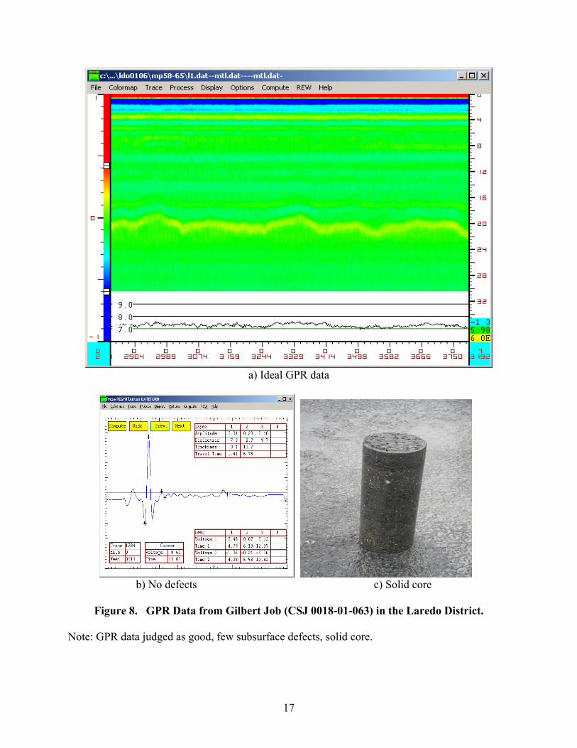
Figure 9 shows data from another perpetual pavement in the Laredo District (CSJ 0017-
08-067); this is known as the Zumwalt 1 job. These data are from the first 1 mile of the project.
The only potential defect in the GPR data is shown in Figure 9(b) as a negative reflection about
mid depth in the asphalt layer. The indication here is that the bottom of the second lift of 1-inch
SF has compaction problems. Also, it is noted that all of the cores taken from this location were
debonded in the middle of the 1-inch SF layer.
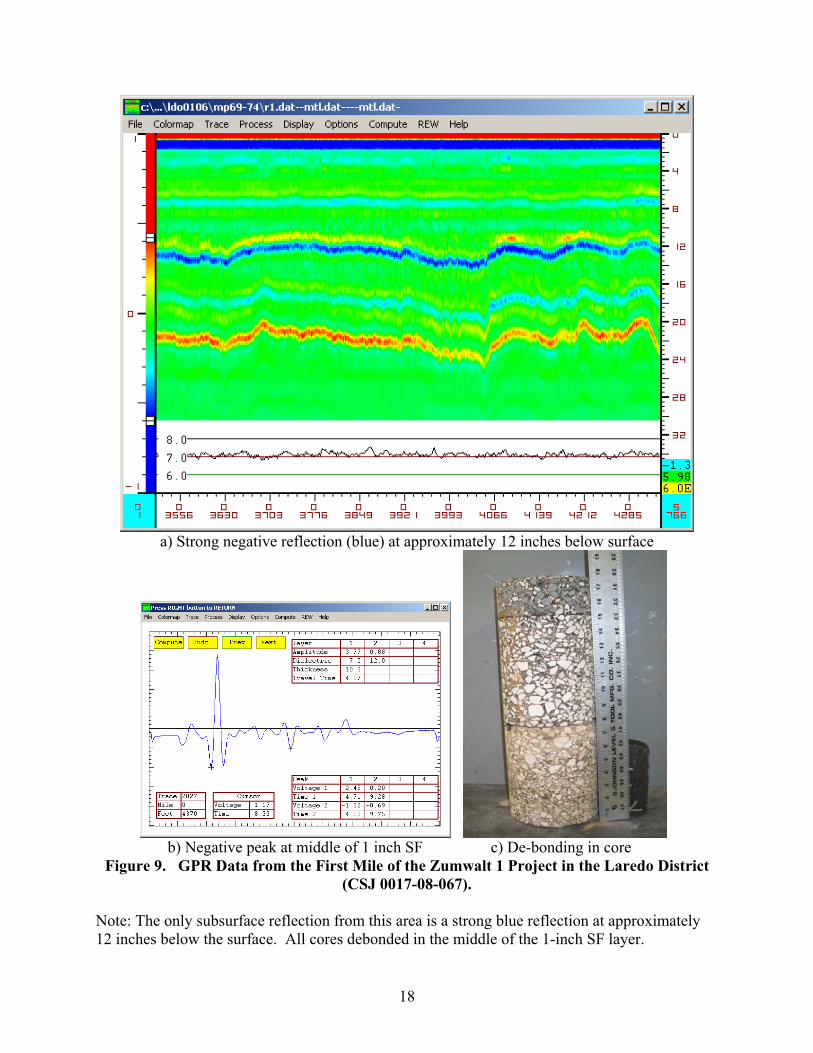
Figure 10 shows GPR data from another section of the Zumwalt 1 job shown in Figure 9.
On this project, the Laredo District lab worked closely with the contractor personnel. In the first
mile, the steel wheel roller was used as the breakdown roller for the 1-inch SF layers; however,
compaction problems were identified. After 1 mile, the district and contractor opted to switch to
using the pneumatic roller as the breakdown roller. For this particular mix on this job, the use of
the pneumatic as the breakdown roller appears to be helping with compaction. As shown in
Figure 10(b) from the first mile of the project, there is a distinct negative reflection in the middle
of the mat; however, after the transition shown in Figure 10(c) the interface reflections are
significantly smaller. This is shown clearly in the upper plot of Figure 10(a); after the first mile,
the blue line in the middle of the mat disappears indicating that the mix is more uniform with
depth.
Figure 11 shows GPR data and field cores from the most recently completed project in
Laredo, CSJ 0018-02-049 (Zumwalt 2). The GPR images from this section are very clean as
17
a) Ideal GPR data
b) No defects c) Solid core
Figure 8. GPR Data from Gilbert Job (CSJ 0018-01-063) in the Laredo District.
Note: GPR data judged as good, few subsurface defects, solid core.
18
a) Strong negative reflection (blue) at approximately 12 inches below surface
b) Negative peak at middle of 1 inch SF c) De-bonding in core
Figure 9. GPR Data from the First Mile of the Zumwalt 1 Project in the Laredo District (CSJ 0017-08-067).
Note: The only subsurface reflection from this area is a strong blue reflection at approximately 12 inches below the surface. All cores debonded in the middle of the 1-inch SF layer.
19
a) GPR data from transition area
b) Low density at bottom of layer c) No major problems after transition
Figure 10. GPR Data from the Transition Section on the Zumwalt 1 Job.
Note: A change in the type of breakdown roller was initiated 1 mile from the start of the project. The steel wheel was used initially; after 1 mile, this was replaced with a pneumatic roller. The GPR indicates a change in compaction levels after 1 mile. The pneumatic compactor appears to produce more uniformly compacted material.
20
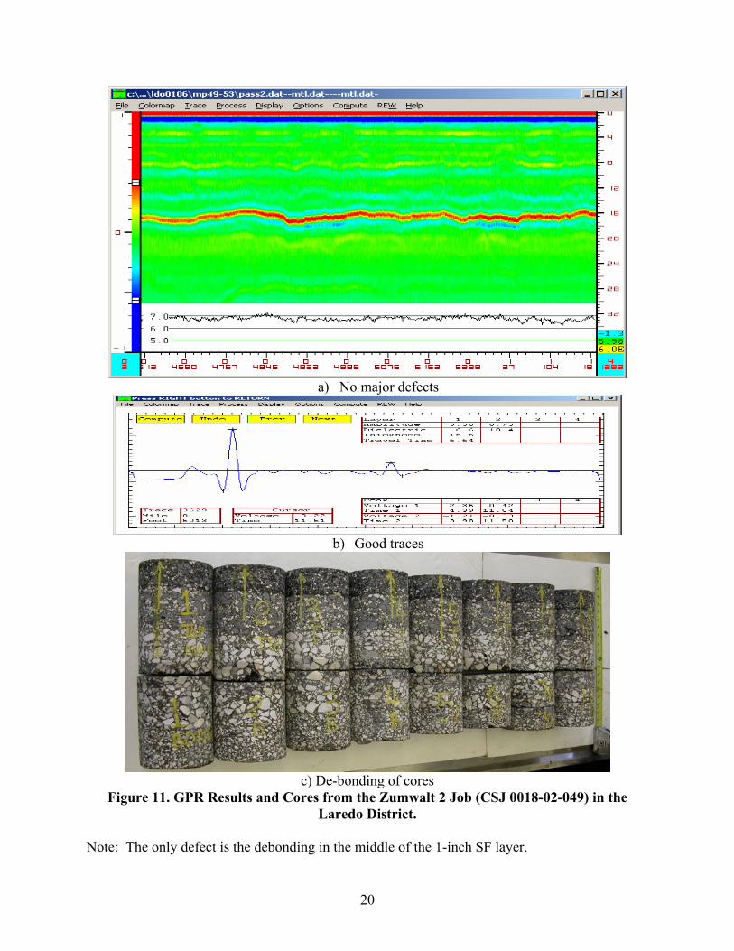
a) No major defects
b) Good traces
c) De-bonding of cores
Figure 11. GPR Results and Cores from the Zumwalt 2 Job (CSJ 0018-02-049) in the Laredo District.
Note: The only defect is the debonding in the middle of the 1-inch SF layer.
21
shown in Figure 11(b), and no major reflections are noted in the middle of the mat. The cores
taken from this section all appear to be in good condition. The only defect in the cores is
debonding in the middle of the 1-inch SF; every core broke at the same location.
In general, the GPR data and field cores obtained from Laredo are more uniform than the
other sections built in Texas. The factors involved in this will be discussed later in this report.
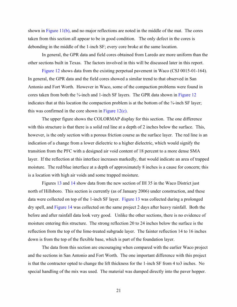
Figure 12 shows data from the existing perpetual pavement in Waco (CSJ 0015-01-164).
In general, the GPR data and the field cores showed a similar trend to that observed in San
Antonio and Fort Worth. However in Waco, some of the compaction problems were found in
cores taken from both the ¾-inch and 1-inch SF layers. The GPR data shown in Figure 12
indicates that at this location the compaction problem is at the bottom of the ¾-inch SF layer;
this was confirmed in the core shown in Figure 12(c).
The upper figure shows the COLORMAP display for this section. The one difference
with this structure is that there is a solid red line at a depth of 2 inches below the surface. This,
however, is the only section with a porous friction course as the surface layer. The red line is an
indication of a change from a lower dielectric to a higher dielectric, which would signify the
transition from the PFC with a designed air void content of 18 percent to a more dense SMA
layer. If the reflection at this interface increases markedly, that would indicate an area of trapped
moisture. The red/blue interface at a depth of approximately 8 inches is a cause for concern; this
is a location with high air voids and some trapped moisture.
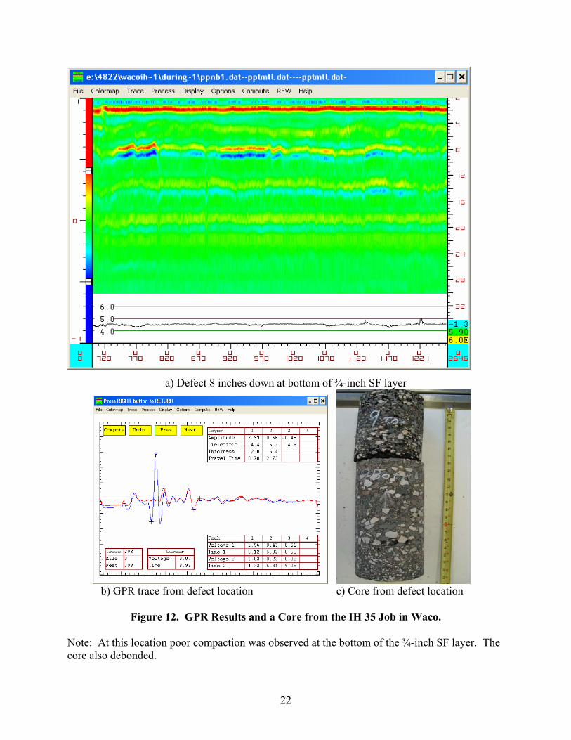
Figures 13 and 14 show data from the new section of IH 35 in the Waco District just
north of Hillsboro. This section is currently (as of January 2006) under construction, and these
data were collected on top of the 1-inch SF layer. Figure 13 was collected during a prolonged
dry spell, and Figure 14 was collected on the same project 2 days after heavy rainfall. Both the
before and after rainfall data look very good. Unlike the other sections, there is no evidence of
moisture entering this structure. The strong reflection 20 to 24 inches below the surface is the
reflection from the top of the lime-treated subgrade layer. The fainter reflection 14 to 16 inches
down is from the top of the flexible base, which is part of the foundation layer.
The data from this section are encouraging when compared with the earlier Waco project
and the sections in San Antonio and Fort Worth. The one important difference with this project
is that the contractor opted to change the lift thickness for the 1-inch SF from 4 to3 inches. No
special handling of the mix was used. The material was dumped directly into the paver hopper.
22
a) Defect 8 inches down at bottom of ¾-inch SF layer
b) GPR trace from defect location c) Core from defect location
Figure 12. GPR Results and a Core from the IH 35 Job in Waco.
Note: At this location poor compaction was observed at the bottom of the ¾-inch SF layer. The core also debonded.
23
a) Ideal data with no obvious defects
b) Ideal traces
Figure 13. GPR Data Collected on the Hillsboro Perpetual Pavement during
Construction. Note: GPR data collected during prolonged dry spell. Data collected on top of the 1-inch SF layer. No defects apparent in this mat.
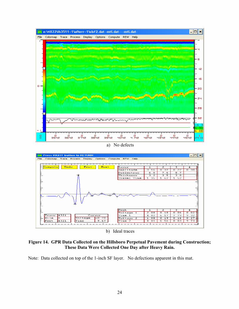
24
a) No defects
b) Ideal traces
Figure 14. GPR Data Collected on the Hillsboro Perpetual Pavement during Construction;
These Data Were Collected One Day after Heavy Rain. Note: Data collected on top of the 1-inch SF layer. No defections apparent in this mat.
25
The pneumatic rollers were not used in the compaction process; only steel wheel rollers were
used.
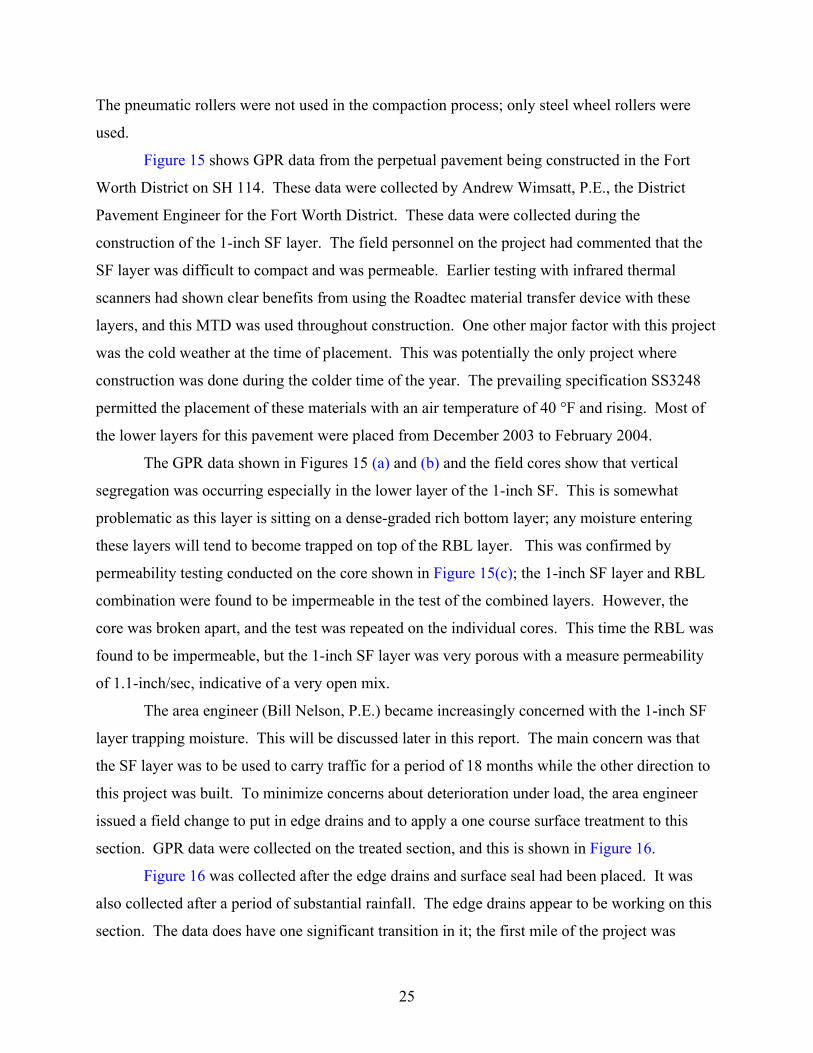
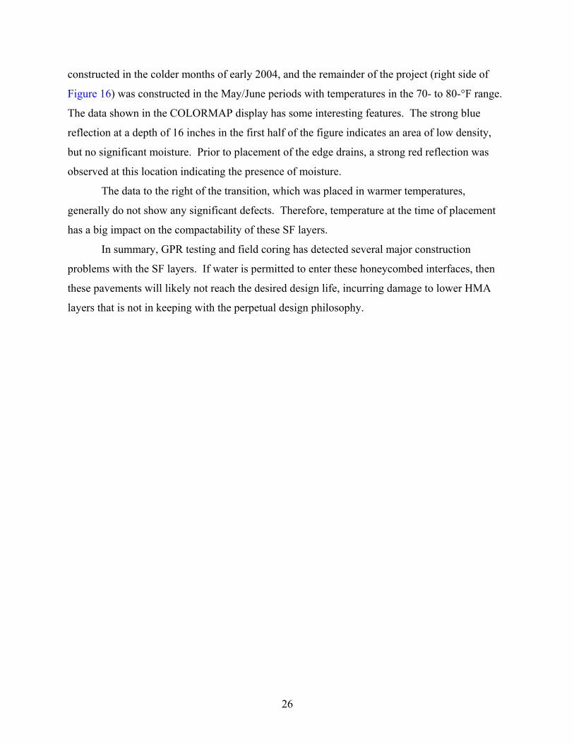
Figure 15 shows GPR data from the perpetual pavement being constructed in the Fort
Worth District on SH 114. These data were collected by Andrew Wimsatt, P.E., the District
Pavement Engineer for the Fort Worth District. These data were collected during the
construction of the 1-inch SF layer. The field personnel on the project had commented that the
SF layer was difficult to compact and was permeable. Earlier testing with infrared thermal
scanners had shown clear benefits from using the Roadtec material transfer device with these
layers, and this MTD was used throughout construction. One other major factor with this project
was the cold weather at the time of placement. This was potentially the only project where
construction was done during the colder time of the year. The prevailing specification SS3248
permitted the placement of these materials with an air temperature of 40 °F and rising. Most of
the lower layers for this pavement were placed from December 2003 to February 2004.
The GPR data shown in Figures 15 (a) and (b) and the field cores show that vertical
segregation was occurring especially in the lower layer of the 1-inch SF. This is somewhat
problematic as this layer is sitting on a dense-graded rich bottom layer; any moisture entering
these layers will tend to become trapped on top of the RBL layer. This was confirmed by
permeability testing conducted on the core shown in Figure 15(c); the 1-inch SF layer and RBL
combination were found to be impermeable in the test of the combined layers. However, the
core was broken apart, and the test was repeated on the individual cores. This time the RBL was
found to be impermeable, but the 1-inch SF layer was very porous with a measure permeability
of 1.1-inch/sec, indicative of a very open mix.
The area engineer (Bill Nelson, P.E.) became increasingly concerned with the 1-inch SF
layer trapping moisture. This will be discussed later in this report. The main concern was that
the SF layer was to be used to carry traffic for a period of 18 months while the other direction to
this project was built. To minimize concerns about deterioration under load, the area engineer
issued a field change to put in edge drains and to apply a one course surface treatment to this
section. GPR data were collected on the treated section, and this is shown in Figure 16.
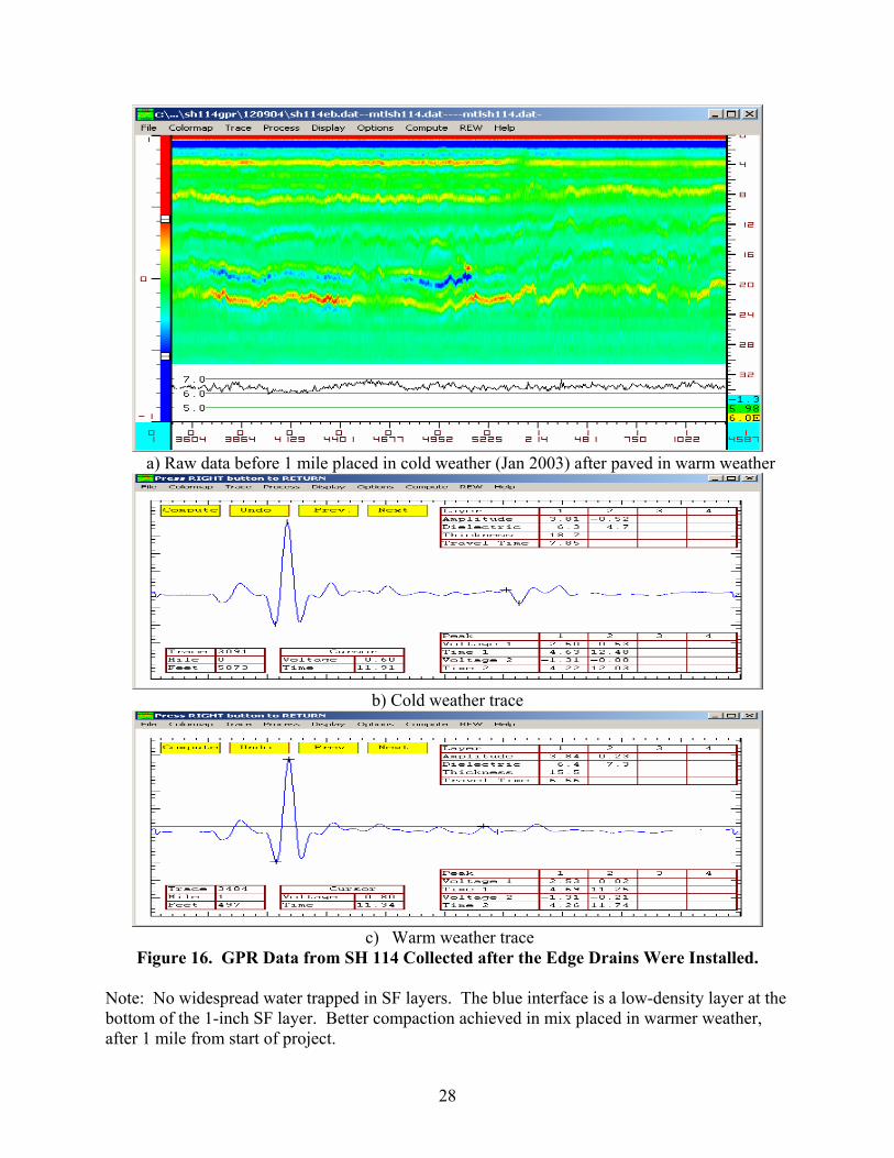
Figure 16 was collected after the edge drains and surface seal had been placed. It was
also collected after a period of substantial rainfall. The edge drains appear to be working on this
section. The data does have one significant transition in it; the first mile of the project was
26
constructed in the colder months of early 2004, and the remainder of the project (right side of
Figure 16) was constructed in the May/June periods with temperatures in the 70- to 80-°F range.
The data shown in the COLORMAP display has some interesting features. The strong blue
reflection at a depth of 16 inches in the first half of the figure indicates an area of low density,
but no significant moisture. Prior to placement of the edge drains, a strong red reflection was
observed at this location indicating the presence of moisture.
The data to the right of the transition, which was placed in warmer temperatures,
generally do not show any significant defects. Therefore, temperature at the time of placement
has a big impact on the compactability of these SF layers.
In summary, GPR testing and field coring has detected several major construction
problems with the SF layers. If water is permitted to enter these honeycombed interfaces, then
these pavements will likely not reach the desired design life, incurring damage to lower HMA
layers that is not in keeping with the perpetual design philosophy.
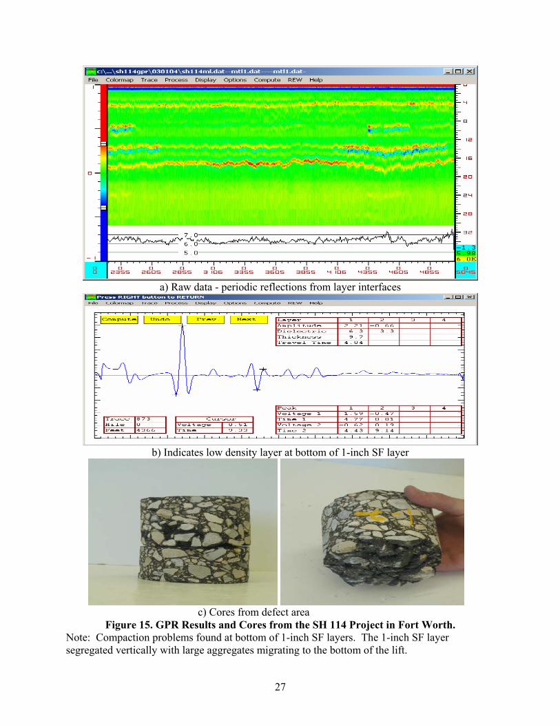
27
a) Raw data - periodic reflections from layer interfaces
b) Indicates low density layer at bottom of 1-inch SF layer
c) Cores from defect area
Figure 15. GPR Results and Cores from the SH 114 Project in Fort Worth. Note: Compaction problems found at bottom of 1-inch SF layers. The 1-inch SF layer segregated vertically with large aggregates migrating to the bottom of the lift.
28
a) Raw data before 1 mile placed in cold weather (Jan 2003) after paved in warm weather
b) Cold weather trace
c) Warm weather trace
Figure 16. GPR Data from SH 114 Collected after the Edge Drains Were Installed. Note: No widespread water trapped in SF layers. The blue interface is a low-density layer at the bottom of the 1-inch SF layer. Better compaction achieved in mix placed in warmer weather, after 1 mile from start of project.
29
FALLING WEIGHT DEFLECTOMETER EVALUATION Background
One of the main purposes of the initial evaluation of the perpetual pavements is to
validate and or revise the design assumption made in the thickness design process. In Texas
flexible pavements are designed using the FPS 19 design system (4). A critical input to this
system is the temperature corrected modulus of each of the pavement layers. This value is
traditionally obtained from FWD testing an existing pavement structure. The MODULUS 6
backcalculation program is used to process FWD data (5). The temperature of the mat at the
time of testing is recorded by the FWD operator. Temperature correction is achieved by
calculating a temperature correction factor using the following equation:
TCF = T ** 2.81 / 200000 (1)
where:
TCF = is the temperature correction factor used to convert the moduli
calculated at field temperatures to 77 °F. A maximum range is used
for TCF from 0.5 and 3.
T = is the temperature measured in the field by the FWD operator. This is
achieved by drilling a hole into the pavement section to the middle of
the asphalt layer at the beginning and end of the FWD data collection.
These numbers are typically averaged to get T.
To obtain a design modulus for any asphalt layer the field backcalculated value is
multiplied by TCF. This temperature corrected modulus is then input to FPS 19 as the design
modulus for that material. Based on numerous field evaluations, TxDOT has historically used
the following values as design moduli for its traditional dense-graded HMA mixes:
Surfacing Mixes Dense-graded fine mixes Type C or D 500 ksi
Base Mixes Dense-graded course mixes Type A or B 400 ksi
30
Historically, TxDOT has not relied on laboratory testing to obtain design moduli values.
This system has worked well over the years, but with the advent of new mixes, several concerns
about the existing materials characterization procedures have been raised. These include:
• How can TxDOT arrive at design moduli for new mix types such as the stone-filled
materials? With the current system, it is essential to construct sections and conduct
FWD testing.
• How can the system account for the move to higher PG grades? The design moduli
described above were developed largely with mixes from the old viscosity system of
AC 10 or AC 20; however, in recent years, new stiffer binders have become common
such as PG 76-22.
• As many of the layers placed in Texas pavement structures are relatively thin, how
well does the backcalculation software do at computing moduli values for layers less
than 3 inches thick (in the current version of MODULUS 6, it is recommended that
the moduli of the asphalt layer be fixed based on prevailing temperature if the mat
thickness is less than 3 inches)?
• With the perpetual pavements consisting of multiple layers of different asphalt mixes
(the Waco sections had five different mixes), how can a backcalculation program be
used to obtain moduli values for each layer?
These are major concerns that will be addressed throughout the course of
Project 0-4822. In general, TxDOT engineers are comfortable with the designs generated by the
FPS 19 design system, and the models within the system have been calibrated based on field
backcalculated material properties. Therefore, in the short term, the urgent need is to
verify/update the design moduli values for the new mixes based on collected FWD data. Later
studies in Project 0-4822 will evaluate the comparison between laboratory and field moduli
values, and the use of more mechanistically based design programs such as the NCHRP 1–37
program.
31
Results from Perpetual Pavements
Falling weight data were collected on six of the perpetual pavements shown in Table 1.
On the Zumwalt 1 and Gilbert jobs in Laredo, data were collected twice (once in the spring and
once during the summer). On all other projects (Zumwalt 2, San Antonio, Waco 1, and
Fort Worth), FWD data were collected once. More data sets will be collected in the future; the
focus of this work was to attempt to collect FWD data in the hotter parts of the year. It was also
important to evaluate the deflection response of the main structural component of this structure,
that being the 1-inch SF layer. In the initial design work, this layer was assumed to have a
temperature corrected modulus value of 500 ksi.
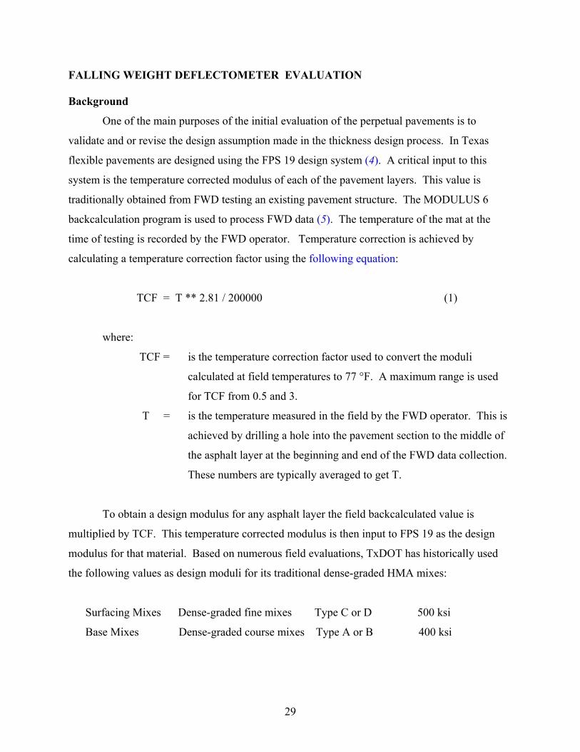
One concern about this system is measuring the temperature of the mat at the time of
testing. Traditionally, TxDOT data collectors drill holes to a depth of 2 inches. With these
perpetual pavements, some with 20 inches of asphalt, a more complete temperature profile is
required. For that, a thermocouple string shown in Figure 17 was developed. A string of six
thermocouples is mounted at a 3-inch spacing on a wooden dowel. This is fitted inside a hole
drilled through the entire asphalt layer. Temperature data with depth are collected regularly
throughout the FWD data collection.
Figure 17. Temperature Probe Installation.
32
Normal TxDOT procedures are followed when testing these perpetual pavements. The
FWD sensors are kept at 1-foot spacings. For long projects, a minimum of 30 drops are
collected.
In processing the FWD data, several assumptions and simplifications were made because
of the limitation of the backcalculation program. The maximum number of layers MODULUS 6
can handle is four. Two of the layers that must be included in the analysis are the foundation
layer and the existing subgrade layer. Therefore the maximum number of layers that can be used
for the asphalt layers is two. This is problematic as the minimum number of different hot mix
layers in a completed perpetual pavement is four (SMA, ¾-inch SF, 1-inch SF and RBL).
Based on the need to evaluate the structural contribution from the 1-inch SF layer, all
efforts were made to isolate that layer as best as possible in the analysis. For example, in the
completed Laredo projects, the SMA layer and ¾-inch SF layer were combined to provide a
6-inch surface layer. The 1-inch SF layer was combined with the RBL to give the second asphalt
layer (for the Gilbert job the thickness would be 10 inches, 8 + 2). The combination of the SF
and RBL layer will provide a composite modulus, which will be conservative for the SF layer as
it is known that the SF layer will have a higher modulus than the RBL layer. In several cases,
the FWD data were collected during construction, so the layer thicknesses used represent the
structure at the time of testing.
The detailed results from the FWD analysis are shown in the appendix for the 10 sets of
data collected. For the San Antonio project three sets of FWD data are given. For the New
Braunfels project, the contractor was having penalty problems related to the measured density of
the original 1-inch SF layers. Midway through the project he opted to change the gradation of
the mix. He added 5 percent field sand to improve mix workability; the mix gradations will be
presented later in this report. The first two sets, Tables A6 and A7, are for the old courser SF
layer; Table A8 is data collected on the revised mix.
The backcalculation results for the 1-inch SF layers are provided below in Table 3. The
test temperature in Table 3 is the average temperature for the SF layer at the time of testing. The
backcalculated moduli values for the upper layers are shown in Table 4. For this analysis the
SMA and ¾-inch SF were combined, therefore, the values in Table 4 are for a composite layer.
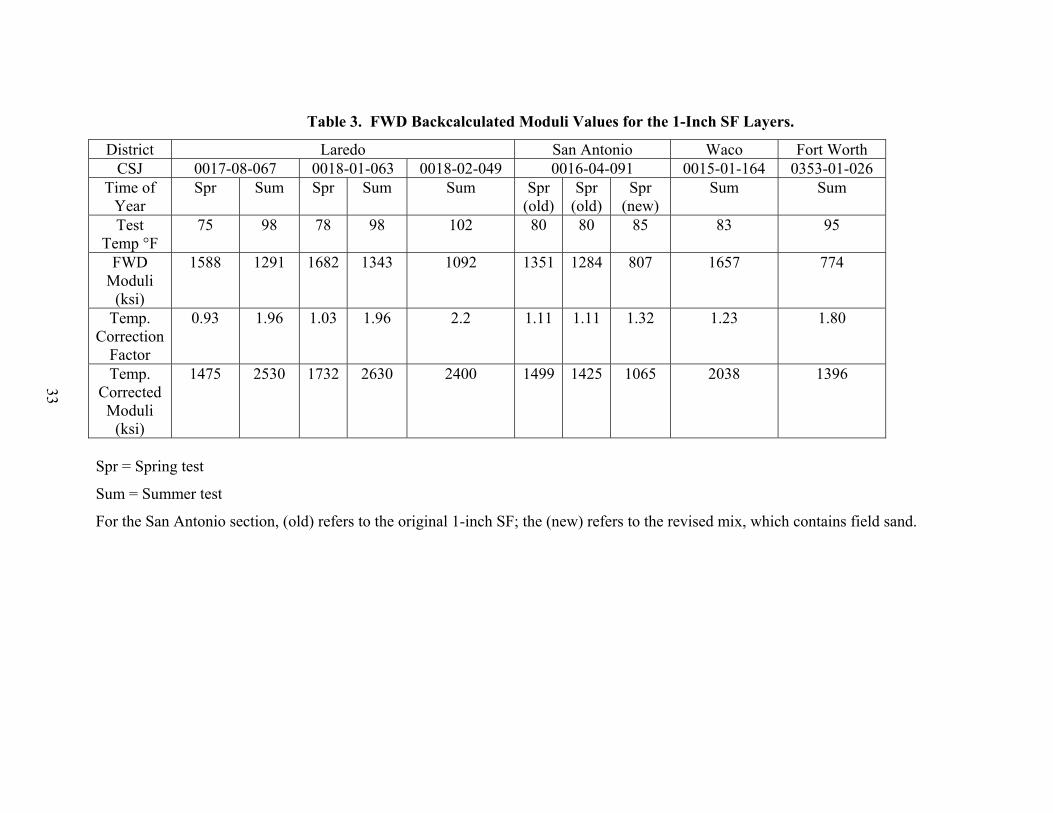
Table 3. FWD Backcalculated Moduli Values for the 1-Inch SF Layers.
District Laredo San Antonio Waco Fort Worth CSJ 0017-08-067 0018-01-063 0018-02-049 0016-04-091 0015-01-164 0353-01-026
Time of Year
Spr Sum Spr Sum Sum Spr (old)
Spr (old)
Spr (new)
Sum Sum
Test Temp °F
75 98 78 98 102 80 80 85 83 95
FWD Moduli
(ksi)
1588 1291 1682 1343 1092 1351 1284 807 1657 774
Temp. Correction
Factor
0.93 1.96 1.03 1.96 2.2 1.11 1.11 1.32 1.23 1.80
Temp. Corrected Moduli
(ksi)
1475 2530 1732 2630 2400 1499 1425 1065 2038 1396
Spr = Spring test
Sum = Summer test
For the San Antonio section, (old) refers to the original 1-inch SF; the (new) refers to the revised mix, which contains field sand.
33
34
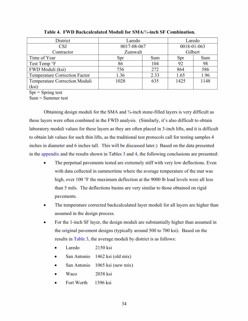
Table 4. FWD Backcalculated Moduli for SMA/¾-inch SF Combination.
District Laredo Laredo CSJ
Contractor 0017-08-067
Zumwalt 0018-01-063
Gilbert Time of Year Spr Sum Spr Sum Test Temp °F 86 104 92 98 FWD Moduli (ksi) 756 272 864 586 Temperature Correction Factor 1.36 2.33 1.65 1.96 Temperature Correction Moduli (ksi)
1028 635 1425 1148
Spr = Spring test Sum = Summer test
Obtaining design moduli for the SMA and ¾-inch stone-filled layers is very difficult as
these layers were often combined in the FWD analysis. (Similarly, it’s also difficult to obtain
laboratory moduli values for these layers as they are often placed in 3-inch lifts, and it is difficult
to obtain lab values for such thin lifts, as the traditional test protocols call for testing samples 4
inches in diameter and 6 inches tall. This will be discussed later.) Based on the data presented
in the appendix and the results shown in Tables 3 and 4, the following conclusions are presented:
• The perpetual pavements tested are extremely stiff with very low deflections. Even
with data collected in summertime where the average temperature of the mat was
high, over 100 °F the maximum deflection at the 9000 lb load levels were all less
than 5 mils. The deflections basins are very similar to those obtained on rigid
pavements.
• The temperature corrected backcalculated layer moduli for all layers are higher than
assumed in the design process.
• For the 1-inch SF layer, the design moduli are substantially higher than assumed in
the original pavement designs (typically around 500 to 700 ksi). Based on the
results in Table 3, the average moduli by district is as follows:
• Laredo 2150 ksi
• San Antonio 1462 ksi (old mix)
• San Antonio 1065 ksi (new mix)
• Waco 2038 ksi
• Fort Worth 1396 ksi
35
• Given that the values in Table 3 are conservative as the analysis combined the SF
and RBL layers to get a lift thickness, a design value of 1000 ksi seems reasonable
for this material.
• For the SMA and ¾-inch SF, only a composite modulus for both layers was
computed from the FWD. The average modulus for the two projects in Laredo
were 830 and 1286 ksi. In the FPS design program, it is also commonplace to use
fixed thicknesses for the upper asphalt layers and use the program to compute the
thickness of the structural layer (the 1-inch SF layer). If this is the case, it seems
reasonable that a design modulus of 750 ksi could be used for the combined upper
layers. (A comparison of SMA and ¾-inch SF layer stiffness will be presented later
in the lab testing results.)
• The GPR results found compaction problems with several of the projects,
particularly with the 1-inch SF layer. This was not found to be directly related to
the stiffness of the layers in that the section with the worst problems, the San
Antonio project, was calculated to have some of the lower in-place stiffness values,
whereas the well compacted sections such as those in Laredo had substantially
higher stiffness. The stiffness values are primarily related to the binder used, the
San Antonio FWD tests we conducted on the 1 inch SF layer which used a PG 64-
22 binder, whereas the Laredo tests we conducted on the completed section with
both PG 76-22 and PG 70-22 binders. The compaction problems appear to be
related to both mix design (gradation and binder content) and construction issues
such as lift thickness, roller sequence, placement temperature, and the use of MTDs.
• Unless the ingress of moisture into the sections with poor compaction is minimized,
then it is predicted that the moduli on the section will decrease with time. The Fort
Worth project with its edge drains and underseal would be predicted to remain
constant, whereas the San Antonio and Waco 1 project would be anticipated to
degrade with time.
36
OBSERVATIONS FROM CORING
Many of the discussions in the GPR section referred to possible problems in several of
the lower lifts of the perpetual pavements built to date in Texas. However, it is critical with an
NDT evaluation to confirm these interpretations with field coring in the impacted area. Photos
of several of the cored pavements are presented in this chapter of the report.
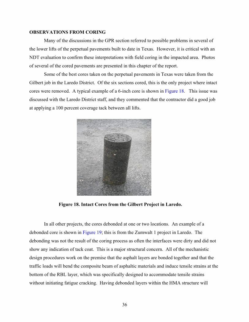
Some of the best cores taken on the perpetual pavements in Texas were taken from the
Gilbert job in the Laredo District. Of the six sections cored, this is the only project where intact
cores were removed. A typical example of a 6-inch core is shown in Figure 18. This issue was
discussed with the Laredo District staff, and they commented that the contractor did a good job
at applying a 100 percent coverage tack between all lifts.
Figure 18. Intact Cores from the Gilbert Project in Laredo.
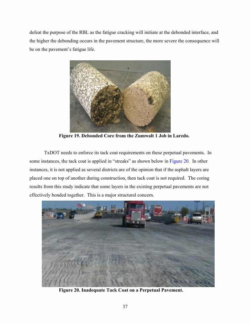
In all other projects, the cores debonded at one or two locations. An example of a
debonded core is shown in Figure 19; this is from the Zumwalt 1 project in Laredo. The
debonding was not the result of the coring process as often the interfaces were dirty and did not
show any indication of tack coat. This is a major structural concern. All of the mechanistic
design procedures work on the premise that the asphalt layers are bonded together and that the
traffic loads will bend the composite beam of asphaltic materials and induce tensile strains at the
bottom of the RBL layer, which was specifically designed to accommodate tensile strains
without initiating fatigue cracking. Having debonded layers within the HMA structure will
37
defeat the purpose of the RBL as the fatigue cracking will initiate at the debonded interface, and
the higher the debonding occurs in the pavement structure, the more severe the consequence will
be on the pavement’s fatigue life.
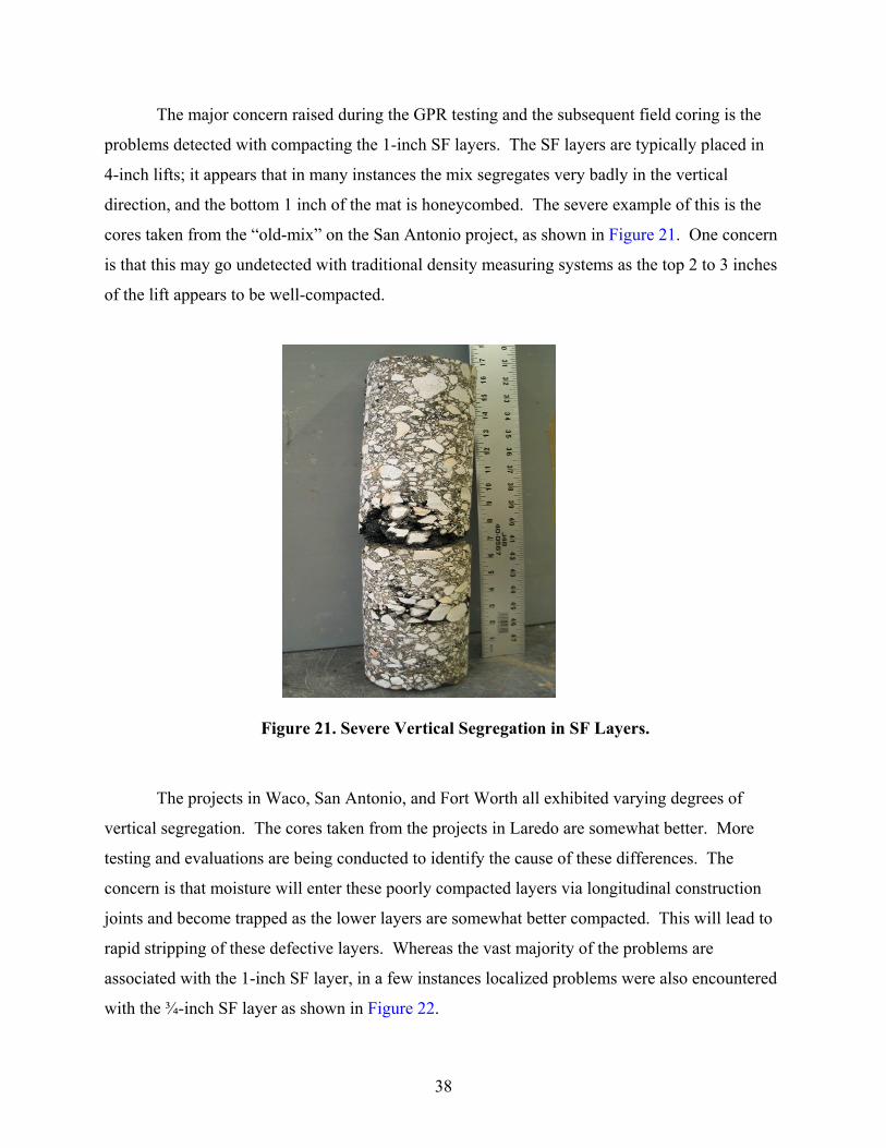
Figure 19. Debonded Core from the Zumwalt 1 Job in Laredo. TxDOT needs to enforce its tack coat requirements on these perpetual pavements. In
some instances, the tack coat is applied in “streaks” as shown below in Figure 20. In other
instances, it is not applied as several districts are of the opinion that if the asphalt layers are
placed one on top of another during construction, then tack coat is not required. The coring
results from this study indicate that some layers in the existing perpetual pavements are not
effectively bonded together. This is a major structural concern.
Figure 20. Inadequate Tack Coat on a Perpetual Pavement.
38
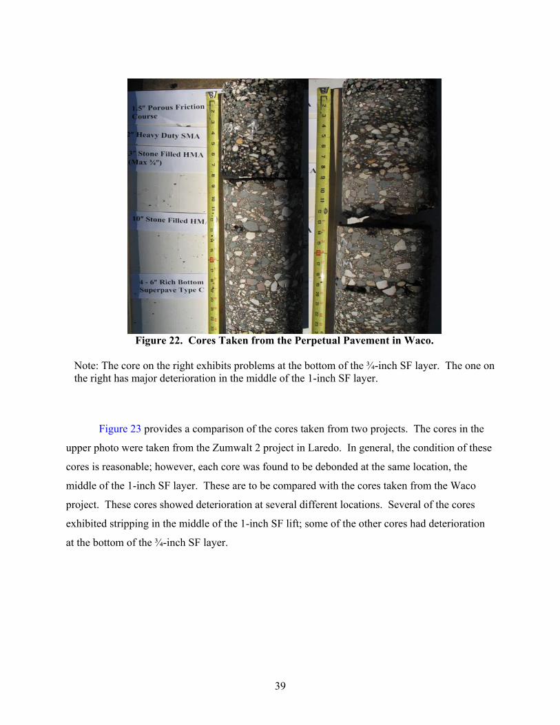
The major concern raised during the GPR testing and the subsequent field coring is the
problems detected with compacting the 1-inch SF layers. The SF layers are typically placed in
4-inch lifts; it appears that in many instances the mix segregates very badly in the vertical
direction, and the bottom 1 inch of the mat is honeycombed. The severe example of this is the
cores taken from the “old-mix” on the San Antonio project, as shown in Figure 21. One concern
is that this may go undetected with traditional density measuring systems as the top 2 to 3 inches
of the lift appears to be well-compacted.
Figure 21. Severe Vertical Segregation in SF Layers.
The projects in Waco, San Antonio, and Fort Worth all exhibited varying degrees of
vertical segregation. The cores taken from the projects in Laredo are somewhat better. More
testing and evaluations are being conducted to identify the cause of these differences. The
concern is that moisture will enter these poorly compacted layers via longitudinal construction
joints and become trapped as the lower layers are somewhat better compacted. This will lead to
rapid stripping of these defective layers. Whereas the vast majority of the problems are
associated with the 1-inch SF layer, in a few instances localized problems were also encountered
with the ¾-inch SF layer as shown in Figure 22.
39
Figure 22. Cores Taken from the Perpetual Pavement in Waco.
Note: The core on the right exhibits problems at the bottom of the ¾-inch SF layer. The one on the right has major deterioration in the middle of the 1-inch SF layer.
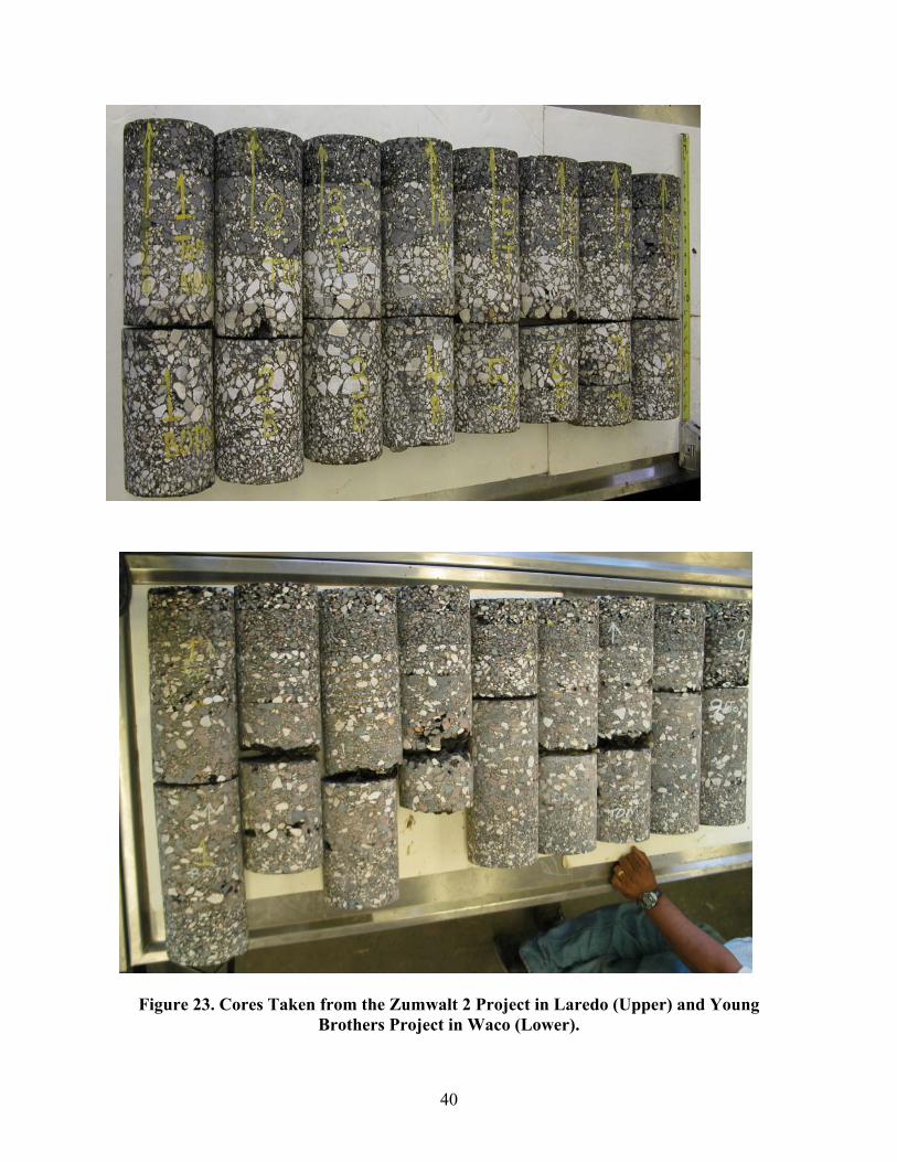
Figure 23 provides a comparison of the cores taken from two projects. The cores in the
upper photo were taken from the Zumwalt 2 project in Laredo. In general, the condition of these
cores is reasonable; however, each core was found to be debonded at the same location, the
middle of the 1-inch SF layer. These are to be compared with the cores taken from the Waco
project. These cores showed deterioration at several different locations. Several of the cores
exhibited stripping in the middle of the 1-inch SF lift; some of the other cores had deterioration
at the bottom of the ¾-inch SF layer.
40
Figure 23. Cores Taken from the Zumwalt 2 Project in Laredo (Upper) and Young Brothers Project in Waco (Lower).
41
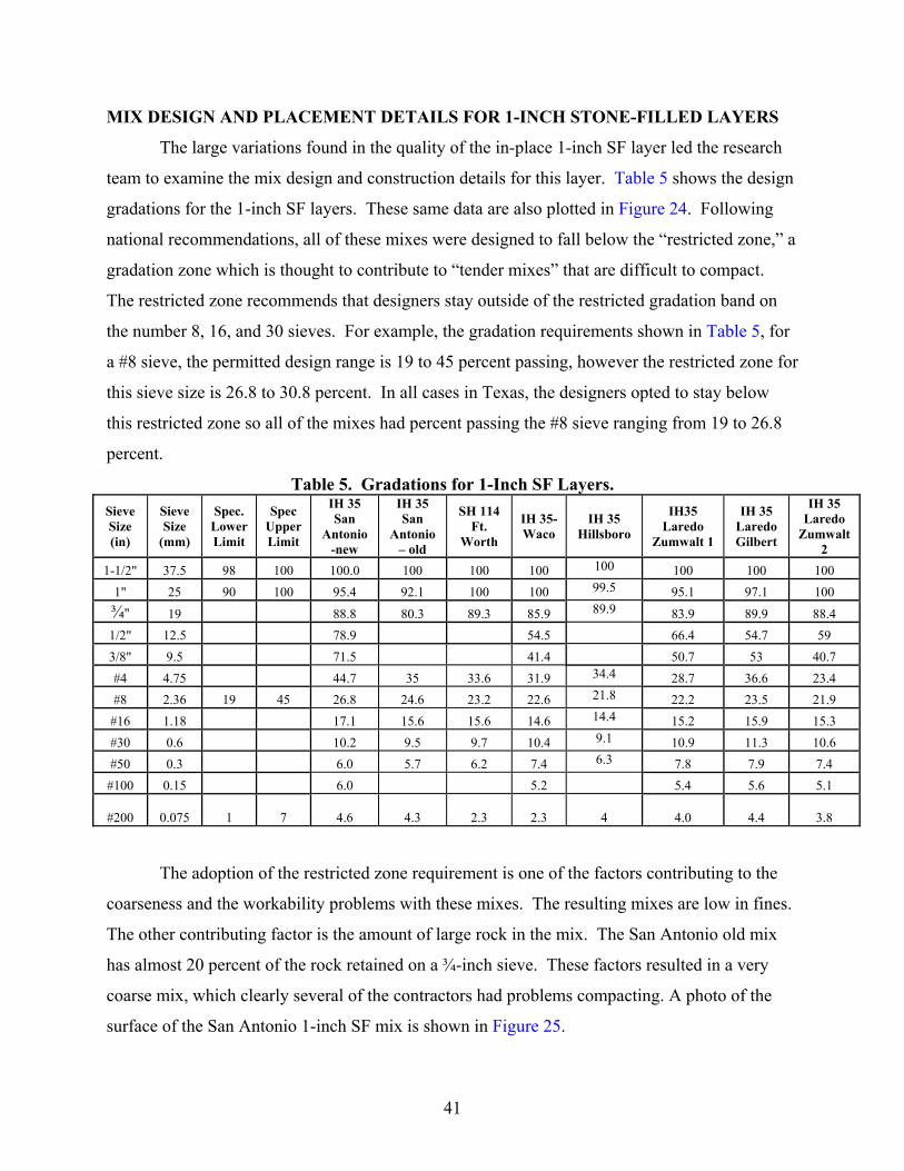
MIX DESIGN AND PLACEMENT DETAILS FOR 1-INCH STONE-FILLED LAYERS
The large variations found in the quality of the in-place 1-inch SF layer led the research
team to examine the mix design and construction details for this layer. Table 5 shows the design
gradations for the 1-inch SF layers. These same data are also plotted in Figure 24. Following
national recommendations, all of these mixes were designed to fall below the “restricted zone,” a
gradation zone which is thought to contribute to “tender mixes” that are difficult to compact.
The restricted zone recommends that designers stay outside of the restricted gradation band on
the number 8, 16, and 30 sieves. For example, the gradation requirements shown in Table 5, for
a #8 sieve, the permitted design range is 19 to 45 percent passing, however the restricted zone for
this sieve size is 26.8 to 30.8 percent. In all cases in Texas, the designers opted to stay below
this restricted zone so all of the mixes had percent passing the #8 sieve ranging from 19 to 26.8
percent.
Table 5. Gradations for 1-Inch SF Layers.
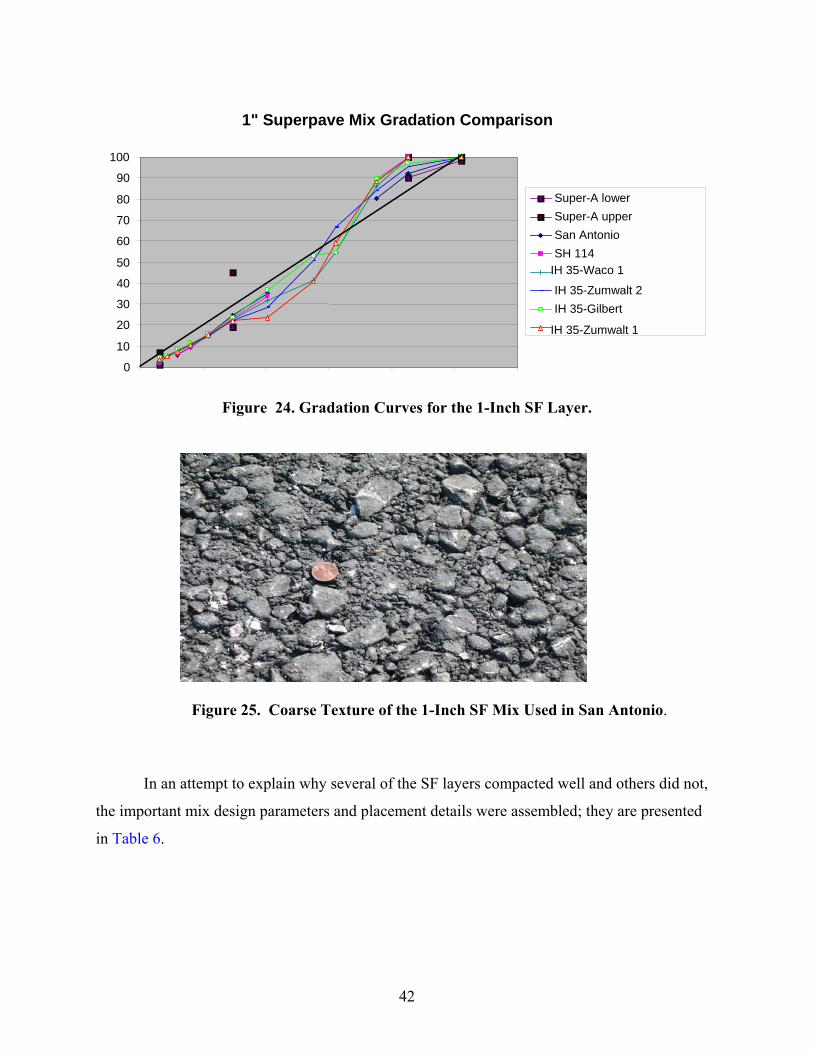
The adoption of the restricted zone requirement is one of the factors contributing to the
coarseness and the workability problems with these mixes. The resulting mixes are low in fines.
The other contributing factor is the amount of large rock in the mix. The San Antonio old mix
has almost 20 percent of the rock retained on a ¾-inch sieve. These factors resulted in a very
coarse mix, which clearly several of the contractors had problems compacting. A photo of the
surface of the San Antonio 1-inch SF mix is shown in Figure 25.
Sieve Size (in)
Sieve Size
(mm)
Spec. Lower Limit
Spec Upper Limit
IH 35 San
Antonio -new
IH 35 San
Antonio – old
SH 114 Ft.
Worth
IH 35-Waco
IH 35
Hillsboro
IH35 Laredo
Zumwalt 1
IH 35 Laredo Gilbert
IH 35 Laredo
Zumwalt 2
1-1/2" 37.5 98 100 100.0 100 100 100 100 100 100 100 1" 25 90 100 95.4 92.1 100 100 99.5 95.1 97.1 100 ¾" 19 88.8 80.3 89.3 85.9 89.9 83.9 89.9 88.4 1/2" 12.5 78.9 54.5 66.4 54.7 59 3/8" 9.5 71.5 41.4 50.7 53 40.7 #4 4.75 44.7 35 33.6 31.9 34.4 28.7 36.6 23.4 #8 2.36 19 45 26.8 24.6 23.2 22.6 21.8 22.2 23.5 21.9 #16 1.18 17.1 15.6 15.6 14.6 14.4 15.2 15.9 15.3 #30 0.6 10.2 9.5 9.7 10.4 9.1 10.9 11.3 10.6 #50 0.3 6.0 5.7 6.2 7.4 6.3 7.8 7.9 7.4
#100 0.15 6.0 5.2 5.4 5.6 5.1
#200 0.075 1 7 4.6 4.3 2.3 2.3
4 4.0 4.4 3.8
42
Figure 24. Gradation Curves for the 1-Inch SF Layer.
Figure 25. Coarse Texture of the 1-Inch SF Mix Used in San Antonio.
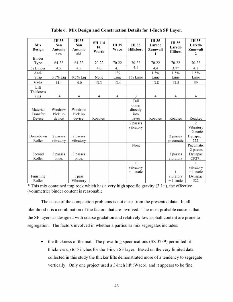
In an attempt to explain why several of the SF layers compacted well and others did not,
the important mix design parameters and placement details were assembled; they are presented
in Table 6.
1" Superpave Mix Gradation Comparison
0 10 20 30 40 50 60 70 80 90
100
Super-A lower Super-A upperSan Antonio SH 114
IH 35-Waco 1 IH 35-Zumwalt 2 IH 35-Gilbert
IH 35-Zumwalt 1
43
Table 6. Mix Design and Construction Details for 1-Inch SF Layer.
Mix Design
IH 35 San
Antonio new
IH 35 San
Antonio old
SH 114 Ft.
Worth
IH 35 Waco
IH 35
Hillsboro
IH 35 Laredo
Zumwalt 1
IH 35 Laredo Gilbert
IH 35 Laredo
Zumwalt 2
Binder Type 64-22 64-22 70-22 70-22
70-22 70-22 70-22 70-22
% Binder 4.5 4.5 4.0 4.1 4.1 4.4 3.7* 4.1 Anti- Strip 0.5% Liq 0.5% Liq None
1% Lime
1% Lime
1.5% Lime
1.5% Lime
1.5% Lime
VMA 14.1 14.0 13.3 13.4 13.8 13.5 59 Lift
Thickness (in) 4 4 4 4
3 4 4 4
Material Transfer Device
Windrow Pick up device
Windrow Pick up device Roadtec
Tail dump
directly into
paver Roadtec Roadtec Roadtec
Breakdown Roller
2 passes vibratory
2 passes vibratory
2 passes vibratory
2 passes
pneumatic
2 Vibratory + 2 static
Dynapac 722
Second Roller
3 passes pnue.
3 passes pnue.
None
3 passes vibratory
Pneumatic 2 passes Dynapac CP271
Finishing Roller
1 pass Vibratory
1 vibratory + 1 static
1 vibratory + 1 static
1 vibratory + 1 static Dynapac
522 * This mix contained trap rock which has a very high specific gravity (3.1+), the effective (volumetric) binder content is reasonable
The cause of the compaction problems is not clear from the presented data. In all
likelihood it is a combination of the factors that are involved. The most probable cause is that
the SF layers as designed with coarse gradation and relatively low asphalt content are prone to
segregation. The factors involved in whether a particular mix segregates includes:
• the thickness of the mat. The prevailing specifications (SS 3239) permitted lift
thickness up to 5 inches for the 1-inch SF layer. Based on the very limited data
collected in this study the thicker lifts demonstrated more of a tendency to segregate
vertically. Only one project used a 3-inch lift (Waco), and it appears to be fine.
44
However, with such limited data and with many confounding issues it is difficult to
provide strong recommendations.
• the temperature at the time of placement, the warmer the better (The Fort Worth
project showed problems; this was the only mix placed in the colder time of year.
However, this may have been resolved with TxDOT’s new 2004 specifications for
performance mixes, which call for surface temperatures of 60 of 70 °F before
placement, which is better than the 40 °F (and rising) ambient temperature
requirement in place for these projects.)
• the coarseness of the mix as measure by the amount of material retained on a 1-inch
sieve, (the coarsest mix was the old San Antonio mix which looked the worst).
• the use of a material transfer device (as used on all of the Laredo projects).
It was difficult to conclude anything about the compaction sequence. One Laredo job
(Gilbert) used the pneumatic as the breakdown roller, but other jobs in Laredo and Waco used
the steel wheel as the breakdown roller with satisfactory results.
DISTRICT EFFORTS TO ADDRESS THE PERMEABILITY ISSUES
The problems of compacting the 1-inch stone-filled layers was recognized by many of the
contractors and districts during the construction process. The Fort Worth District was very
concerned about the permeability of its structure. With its construction sequence, the initial
intention was to place all of the stone-filled layers and then let the traffic drive on the section for
a period of 12 to 18 months while the other side of the four-lane divided highway was
reconstructed. However, it was noted that during periods of heavy rainfall that little water would
flow off the edge of the pavement; most of it appeared to be entering the SF layers. This
reinforced the concerns that had already been raised from the GPR data shown earlier in Figure
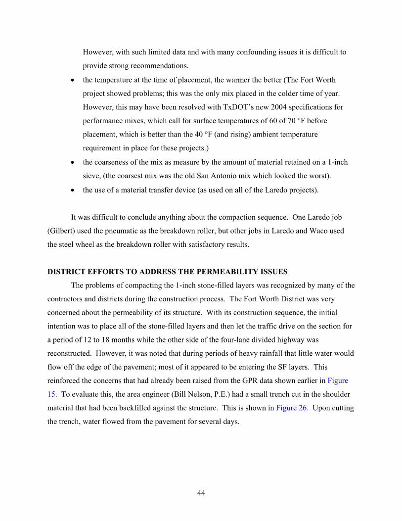
15. To evaluate this, the area engineer (Bill Nelson, P.E.) had a small trench cut in the shoulder
material that had been backfilled against the structure. This is shown in Figure 26. Upon cutting
the trench, water flowed from the pavement for several days.
45
Figure 26. Releasing Trapped Water from the Stone-Filled Asphalt Layers on SH 114.
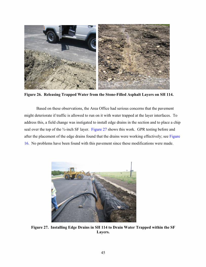
Based on these observations, the Area Office had serious concerns that the pavement
might deteriorate if traffic is allowed to run on it with water trapped at the layer interfaces. To
address this, a field change was instigated to install edge drains in the section and to place a chip
seal over the top of the ¾-inch SF layer. Figure 27 shows this work. GPR testing before and
after the placement of the edge drains found that the drains were working effectively; see Figure
16. No problems have been found with this pavement since these modifications were made.
Figure 27. Installing Edge Drains in SH 114 to Drain Water Trapped within the SF
Layers.

46
SUMMARY
In summary, it is concluded that the design recommendations of the 1-inch SF mix should be
revisited on future perpetual pavement design projects. TxDOT should explore other design
options to minimize the potential for having mixes than cannot be adequately compacted. Many
options exist including:
• adding more asphalt to these mixes, as long as they pass the Hamburg requirement;
• adding more fines, disregarding the restricted zone concept;
• replacing the 1-inch SF with a ¾-inch SF; and
• changing from the SF to a more dense-graded mix.
These options will be explored in the second year of this project. It will be necessary to
evaluate both the mix design and structural design implications of changing mixes.
47
CHAPTER 3
LABORATORY TESTING
The cores taken from the perpetual pavements were returned to TTI for laboratory
testing. This work is ongoing and only preliminary results will be presented here. Efforts were
made to characterize the engineering properties of the field cores. This included validating the
mixture design tests, such as the Hamburg and the Overlay Tester, and also measuring the
dynamic modulus (DM) values. The DM values are required for the new generation of
mechanistic empirical design programs. However, in addition, efforts were aimed at a first order
comparison of the laboratory moduli with the moduli backcalculated from the FWD.
HAMBURG WHEEL TRACKING TEST
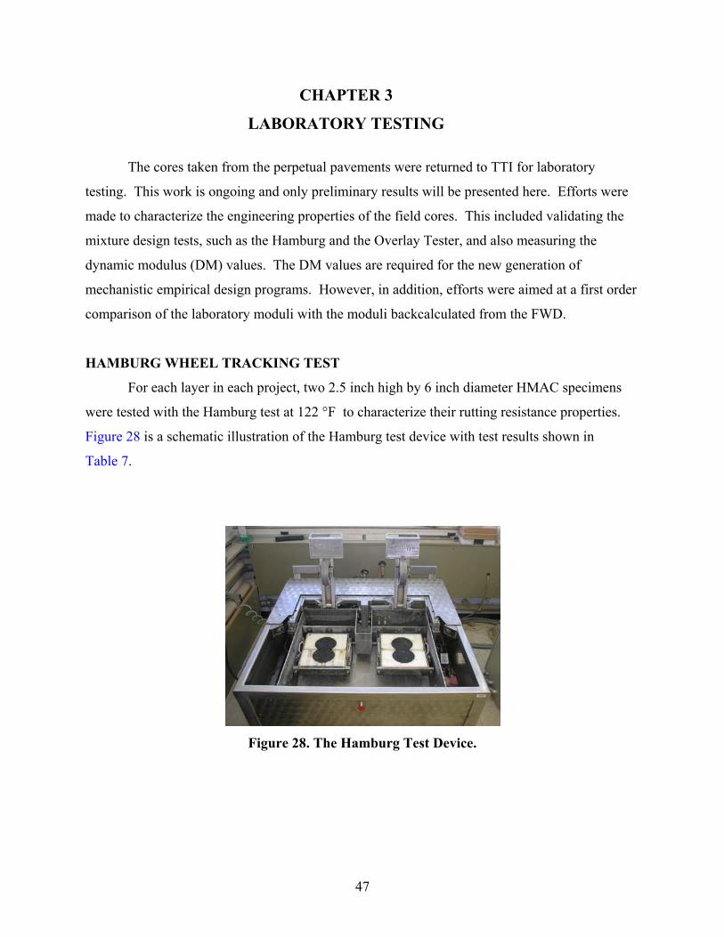
For each layer in each project, two 2.5 inch high by 6 inch diameter HMAC specimens
were tested with the Hamburg test at 122 °F to characterize their rutting resistance properties.
Figure 28 is a schematic illustration of the Hamburg test device with test results shown in
Table 7.
Figure 28. The Hamburg Test Device.
48
The test loading parameters for the Hamburg test were as follows:
• Load: 705 N (158-lb force)
• Number of passes: 20,000
• Test condition/temperature: Under water at 50 °C (122 °F)
• Terminal rutting failure criterion: 0.5 inch (12.5 mm)
• HMAC specimen size: 6-inch diameter by 2.5 inch high
OVERLAY TESTER
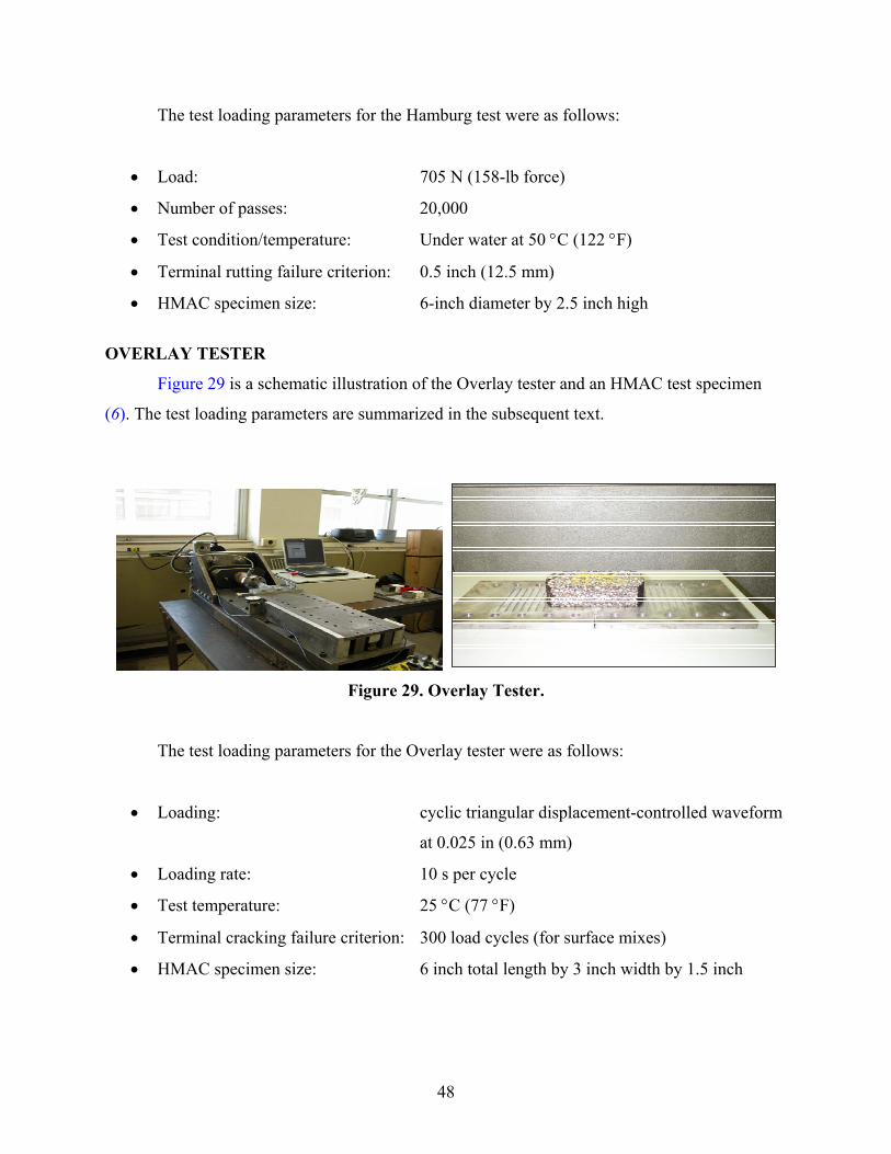
Figure 29 is a schematic illustration of the Overlay tester and an HMAC test specimen
(6). The test loading parameters are summarized in the subsequent text.
Figure 29. Overlay Tester.
The test loading parameters for the Overlay tester were as follows:
• Loading: cyclic triangular displacement-controlled waveform
at 0.025 in (0.63 mm)
• Loading rate: 10 s per cycle
• Test temperature: 25 °C (77 °F)
• Terminal cracking failure criterion: 300 load cycles (for surface mixes)
• HMAC specimen size: 6 inch total length by 3 inch width by 1.5 inch
49
The overlay tester was used to characterize the cracking potential of the mixes at an
ambient temperature of 77 °F. The overlay tester is currently not part of the TxDOT’s mix
design procedure, so the results were included for comparison purposes. Cracking resistance is
not critical for the stone-filled layers (assuming they are bonded together) as these are designed
for rut resistance. However, the SMA mixes and the RBL layers must have good crack
resistance. The RBL layer is supposedly designed to be the fatigue-resistant layer whereas the
SMA is the wearing surface. Work overseas primarily by Nunn and Ferne in England has
reported that the major performance problem with full-depth pavements in the UK has been top
down cracking (7). As the SMA is the surfacing mix for most of the perpetual pavements in
Texas, it is essential that this mix has both good rutting and cracking resistance. Good cracking
resistance will be to minimize the potential risk of top down cracking. TTI has tested numerous
SMA mixes from around Texas, and to date all of these have passed both the Hamburg and
Overlay Tester (>300 cycles to failure) requirements.
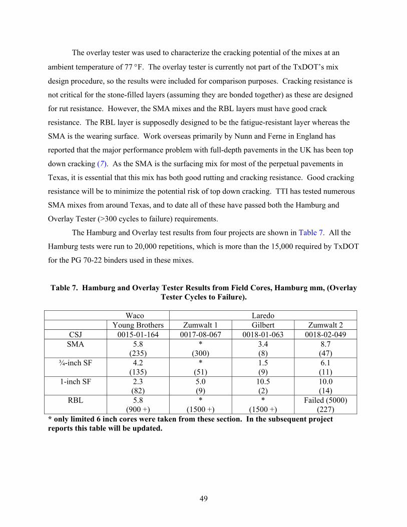
The Hamburg and Overlay test results from four projects are shown in Table 7. All the
Hamburg tests were run to 20,000 repetitions, which is more than the 15,000 required by TxDOT
for the PG 70-22 binders used in these mixes.
Table 7. Hamburg and Overlay Tester Results from Field Cores, Hamburg mm, (Overlay Tester Cycles to Failure).
Waco Laredo
Young Brothers Zumwalt 1 Gilbert Zumwalt 2 CSJ 0015-01-164 0017-08-067 0018-01-063 0018-02-049
SMA 5.8 (235)
* (300)
3.4 (8)
8.7 (47)
¾-inch SF 4.2 (135)
* (51)
1.5 (9)
6.1 (11)
1-inch SF 2.3 (82)
5.0 (9)
10.5 (2)
10.0 (14)
RBL 5.8 (900 +)
* (1500 +)
* (1500 +)
Failed (5000) (227)
* only limited 6 inch cores were taken from these section. In the subsequent project reports this table will be updated.
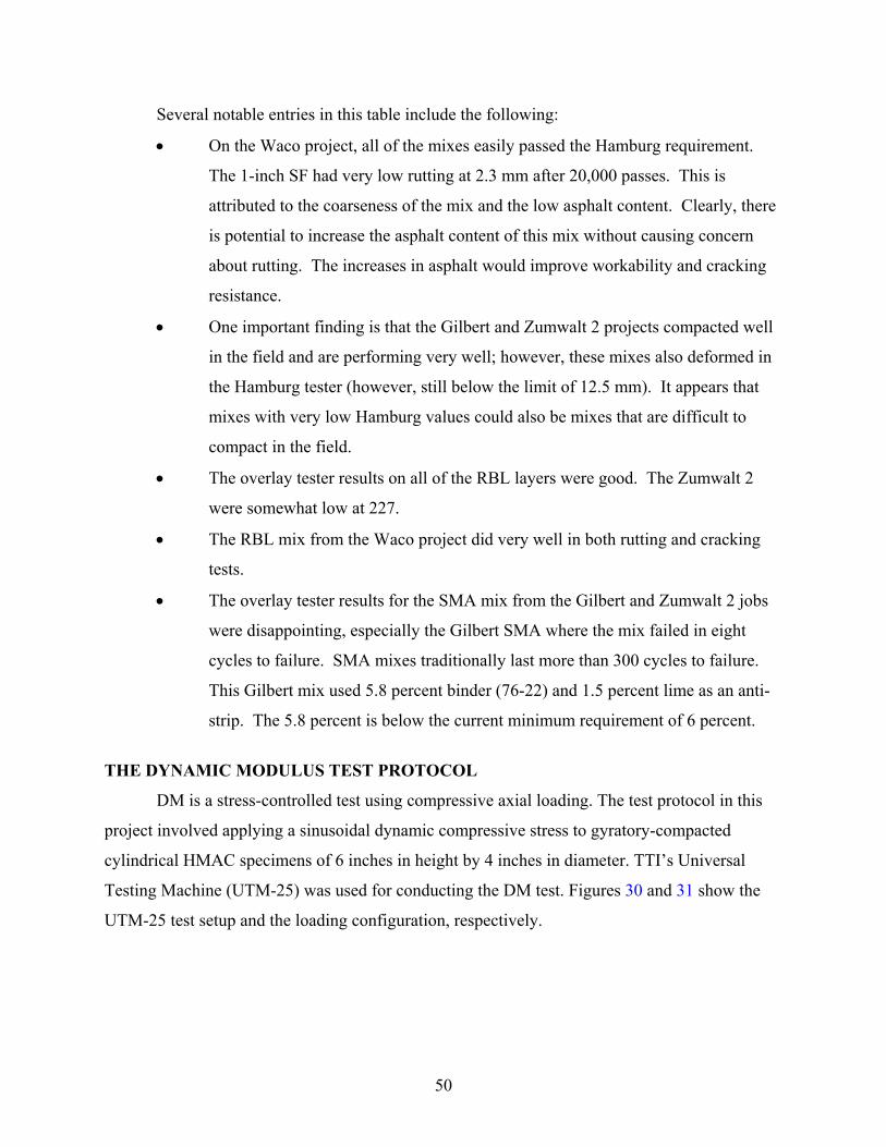
50
Several notable entries in this table include the following:
• On the Waco project, all of the mixes easily passed the Hamburg requirement.
The 1-inch SF had very low rutting at 2.3 mm after 20,000 passes. This is
attributed to the coarseness of the mix and the low asphalt content. Clearly, there
is potential to increase the asphalt content of this mix without causing concern
about rutting. The increases in asphalt would improve workability and cracking
resistance.
• One important finding is that the Gilbert and Zumwalt 2 projects compacted well
in the field and are performing very well; however, these mixes also deformed in
the Hamburg tester (however, still below the limit of 12.5 mm). It appears that
mixes with very low Hamburg values could also be mixes that are difficult to
compact in the field.
• The overlay tester results on all of the RBL layers were good. The Zumwalt 2
were somewhat low at 227.
• The RBL mix from the Waco project did very well in both rutting and cracking
tests.
• The overlay tester results for the SMA mix from the Gilbert and Zumwalt 2 jobs
were disappointing, especially the Gilbert SMA where the mix failed in eight
cycles to failure. SMA mixes traditionally last more than 300 cycles to failure.
This Gilbert mix used 5.8 percent binder (76-22) and 1.5 percent lime as an anti-
strip. The 5.8 percent is below the current minimum requirement of 6 percent.
THE DYNAMIC MODULUS TEST PROTOCOL
DM is a stress-controlled test using compressive axial loading. The test protocol in this
project involved applying a sinusoidal dynamic compressive stress to gyratory-compacted
cylindrical HMAC specimens of 6 inches in height by 4 inches in diameter. TTI’s Universal
Testing Machine (UTM-25) was used for conducting the DM test. Figures 30 and 31 show the
UTM-25 test setup and the loading configuration, respectively.
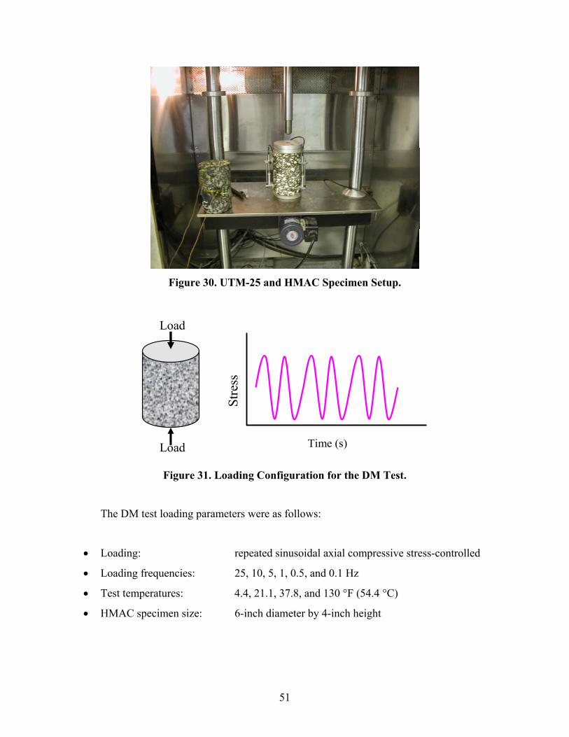
51
Figure 30. UTM-25 and HMAC Specimen Setup.
Load
Load
Time (s)
Stre
ss
Figure 31. Loading Configuration for the DM Test.
The DM test loading parameters were as follows:
• Loading: repeated sinusoidal axial compressive stress-controlled
• Loading frequencies: 25, 10, 5, 1, 0.5, and 0.1 Hz
• Test temperatures: 4.4, 21.1, 37.8, and 130 °F (54.4 °C)
• HMAC specimen size: 6-inch diameter by 4-inch height
52
The stress level for conducting the DM test was chosen in order to maintain the measured
resilient strain (recoverable) within 50 to 150 microstrain consistent with the TP 62-03 test
protocol (AASHTO 2003). The order for conducting each test sequence was from the lowest to
the highest temperature and the highest to the lowest frequency of loading at each temperature to
minimize HMAC specimen damage. For each temperature-frequency test sequence, the test
terminates automatically when a preset number of load cycles have been reached.
THE DYNAMIC MODULUS TEST RESULTS
The typical parameters that are computed from DM testing are the complex modulus
(|E*|) and the phase angle (δ) that characterizes the HMAC visco-elastic properties. The |E*|
data are then used for generation of a HMAC master-curve for pavement performance prediction
in new design programs. This |E*| is a function of the storage (elastic) modulus (E′ ) and loss
(viscous) modulus (E″), and is represented as shown in Equation 2:
0
0|*|εσ
=E (2)
δCosEE |*|'= , δSinEE |*|"= (3)
where:
|E*| = dynamic complex modulus (psi)
0σ = axial stress (psi)
0ε = axial strain (in/in)
E′ , E″ = storage (elastic) and loss (viscous) modulus, respectively (psi)
δ = phase angle (°)
A typical set of data from a DM test is shown below in Table 8. These data are from
laboratory prepared samples for the 1-inch SF mix from the new project in Waco.
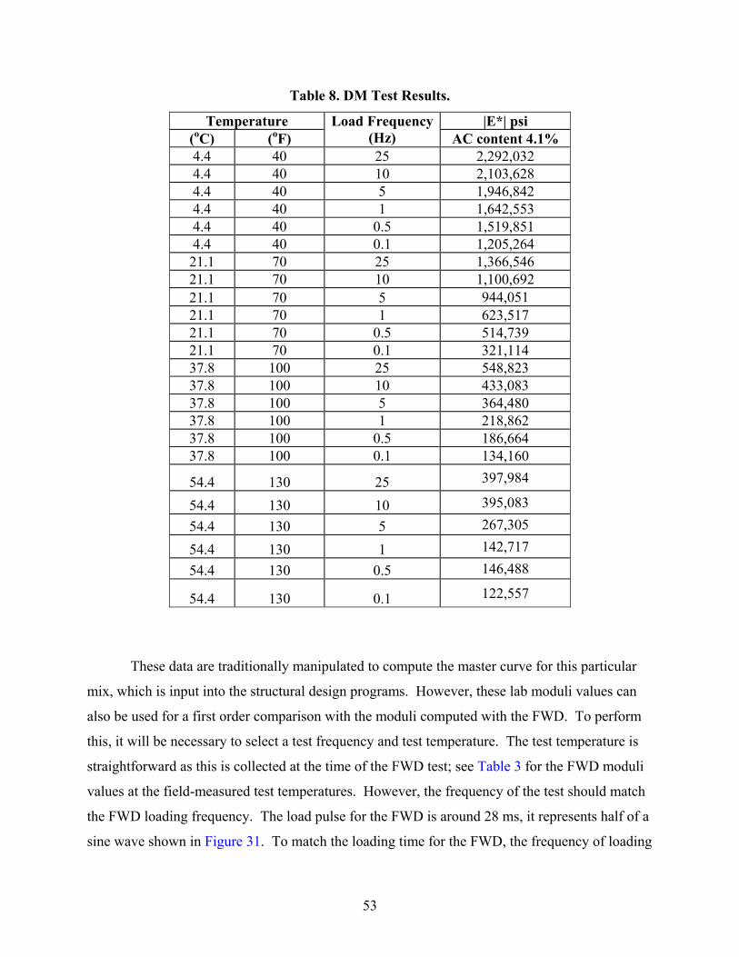
53
Table 8. DM Test Results.
Temperature |E*| psi (oC) (oF)
Load Frequency (Hz) AC content 4.1%
4.4 40 25 2,292,032 4.4 40 10 2,103,628 4.4 40 5 1,946,842 4.4 40 1 1,642,553 4.4 40 0.5 1,519,851 4.4 40 0.1 1,205,264 21.1 70 25 1,366,546 21.1 70 10 1,100,692 21.1 70 5 944,051 21.1 70 1 623,517 21.1 70 0.5 514,739 21.1 70 0.1 321,114 37.8 100 25 548,823 37.8 100 10 433,083 37.8 100 5 364,480 37.8 100 1 218,862 37.8 100 0.5 186,664 37.8 100 0.1 134,160
54.4 130 25 397,984
54.4 130 10 395,083 54.4 130 5 267,305
54.4 130 1 142,717 54.4 130 0.5 146,488
54.4 130 0.1 122,557
These data are traditionally manipulated to compute the master curve for this particular
mix, which is input into the structural design programs. However, these lab moduli values can
also be used for a first order comparison with the moduli computed with the FWD. To perform
this, it will be necessary to select a test frequency and test temperature. The test temperature is
straightforward as this is collected at the time of the FWD test; see Table 3 for the FWD moduli
values at the field-measured test temperatures. However, the frequency of the test should match
the FWD loading frequency. The load pulse for the FWD is around 28 ms, it represents half of a
sine wave shown in Figure 31. To match the loading time for the FWD, the frequency of loading
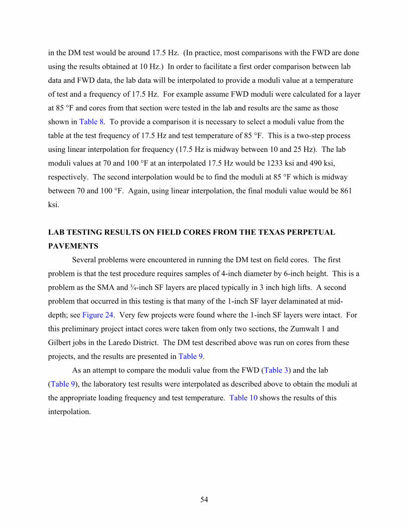
54
in the DM test would be around 17.5 Hz. (In practice, most comparisons with the FWD are done
using the results obtained at 10 Hz.) In order to facilitate a first order comparison between lab
data and FWD data, the lab data will be interpolated to provide a moduli value at a temperature
of test and a frequency of 17.5 Hz. For example assume FWD moduli were calculated for a layer
at 85 °F and cores from that section were tested in the lab and results are the same as those
shown in Table 8. To provide a comparison it is necessary to select a moduli value from the
table at the test frequency of 17.5 Hz and test temperature of 85 °F. This is a two-step process
using linear interpolation for frequency (17.5 Hz is midway between 10 and 25 Hz). The lab
moduli values at 70 and 100 °F at an interpolated 17.5 Hz would be 1233 ksi and 490 ksi,
respectively. The second interpolation would be to find the moduli at 85 °F which is midway
between 70 and 100 °F. Again, using linear interpolation, the final moduli value would be 861
ksi.
LAB TESTING RESULTS ON FIELD CORES FROM THE TEXAS PERPETUAL
PAVEMENTS
Several problems were encountered in running the DM test on field cores. The first
problem is that the test procedure requires samples of 4-inch diameter by 6-inch height. This is a
problem as the SMA and ¾-inch SF layers are placed typically in 3 inch high lifts. A second
problem that occurred in this testing is that many of the 1-inch SF layer delaminated at mid-
depth; see Figure 24. Very few projects were found where the 1-inch SF layers were intact. For
this preliminary project intact cores were taken from only two sections, the Zumwalt 1 and
Gilbert jobs in the Laredo District. The DM test described above was run on cores from these
projects, and the results are presented in Table 9.
As an attempt to compare the moduli value from the FWD (Table 3) and the lab
(Table 9), the laboratory test results were interpolated as described above to obtain the moduli at
the appropriate loading frequency and test temperature. Table 10 shows the results of this
interpolation.
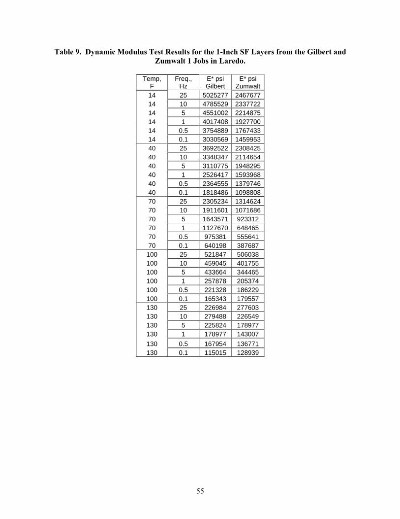
55
Table 9. Dynamic Modulus Test Results for the 1-Inch SF Layers from the Gilbert and Zumwalt 1 Jobs in Laredo.
Temp,
F Freq.,
Hz E* psi Gilbert
E* psi Zumwalt
14 25 5025277 246767714 10 4785529 233772214 5 4551002 221487514 1 4017408 192770014 0.5 3754889 176743314 0.1 3030569 145995340 25 3692522 230842540 10 3348347 211465440 5 3110775 194829540 1 2526417 159396840 0.5 2364555 137974640 0.1 1818486 109880870 25 2305234 131462470 10 1911601 107168670 5 1643571 923312 70 1 1127670 648465 70 0.5 975381 555641 70 0.1 640198 387687
100 25 521847 506038 100 10 459045 401755 100 5 433664 344465 100 1 257878 205374 100 0.5 221328 186229 100 0.1 165343 179557 130 25 226984 277603 130 10 279488 226549 130 5 225824 178977 130 1 178977 143007 130 0.5 167954 136771 130 0.1 115015 128939
56
Table 10. Comparison of Lab and Field Moduli for the 1-Inch SF Layer from the Laredo District.
CSJ Contractor Field Test temp
(°F)
Lab Modulus
(ksi)
Field Modulus
(ksi)
0011-01-063 Gilbert 78 1676 1682
0011-01-063 Gilbert 98 598 1343
0017-08-067 Zumwalt 75 1068 1588
0017-08-067 Zumwalt 98 502 1291
There are numerous assumptions in making a first order comparison such as this. For
example, the DM test is an unconfined test whereas the samples are highly confined in the field.
However, based on this preliminary analysis, the following conclusions are drawn:
• The moduli values obtained from the FWD in the field are in all cases higher than the
values measured in the lab.
• The FWD moduli are significantly higher (by at least a factor of 2) at the higher
temperatures.
• The values obtained at the lower temperatures are closer.
The one surprising feature of monitoring these perpetual pavements in Laredo was the
very small impact that layer temperature had on the overall pavement deflection. As shown in
the Appendix, the average deflection on the Gilbert section only increased from 3.79 to 4.53 mils
when the temperature increased from the 70 °F to close to 100 °F. This small increase is related
to the PG grade of the binder, possibly the use of 1.5 percent lime and the coarseness of the
mixes. This high field stiffness at high temperatures has not been traditionally observed on
other mixes placed in Texas.
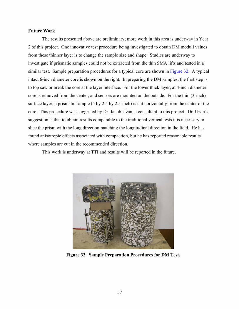
57
Future Work
The results presented above are preliminary; more work in this area is underway in Year
2 of this project. One innovative test procedure being investigated to obtain DM moduli values
from these thinner layer is to change the sample size and shape. Studies are underway to
investigate if prismatic samples could not be extracted from the thin SMA lifts and tested in a
similar test. Sample preparation procedures for a typical core are shown in Figure 32. A typical
intact 6-inch diameter core is shown on the right. In preparing the DM samples, the first step is
to top saw or break the core at the layer interface. For the lower thick layer, at 4-inch diameter
core is removed from the center, and sensors are mounted on the outside. For the thin (3-inch)
surface layer, a prismatic sample (5 by 2.5 by 2.5-inch) is cut horizontally from the center of the
core. This procedure was suggested by Dr. Jacob Uzan, a consultant to this project. Dr. Uzan’s
suggestion is that to obtain results comparable to the traditional vertical tests it is necessary to
slice the prism with the long direction matching the longitudinal direction in the field. He has
found anisotropic effects associated with compaction, but he has reported reasonable results
where samples are cut in the recommended direction.
This work is underway at TTI and results will be reported in the future.
Figure 32. Sample Preparation Procedures for DM Test.

59
CHAPTER 4
CONCLUSIONS AND RECOMMENDATIONS The conclusions from this project are as follows:
• The 1-inch SF layers are prone to vertical segregation. Several of the sections were
found to have severe honeycombing at the bottom of the lifts. These mixes are
excessively coarse with low asphalt binder contents around 4 percent.
• The cause of the segregation was thought primarily due to the coarseness of the mix
design but also somewhat related to construction conditions. Clearly, the mix is more
difficult to compact in cooler weather (as experienced in Fort Worth) and in thicker
lifts. All of these jobs were let with the requirement that the mix can be placed with
air temperatures of 40 °F and above. This problem will be eliminated on future
projects with the new 2004 specification, which specifies a roadway surface
temperature of 60 °F.
• The impact rolling sequence could not be validated. Using the pneumatic as the
breakdown roller appeared to help on one project, but satisfactory results were also
obtained with only steel-wheel compaction.
• Based on the Laredo experience, the use of the Roadtec MTD appeared to help in
mixture uniformity.
• In general, few problems were found with either the SMA or ¾-inch SF layers.
• Full depth cores were obtained from only one of the projects, the Gilbert job in
Laredo. In all other projects, the cores debonded at one or two layer interfaces.
• The structural strength of the foundation layers varied substantially from district to
district. The Waco District builds a foundation layer with lime-treated subgrade and
6 inches of flexible base. Other districts place the asphalt directly on top of clay soils
treated with low levels of lime.
• Structural testing with the FWD found that these pavement structures are very stiff;
the measured deflections are close to the level found with thick concrete pavements.
Researchers also noted that even when testing in the summer months, the pavement
deflections did not increase significantly.
60
• The design moduli for both the SMA and stone-filled layers can be increased
significantly in future FPS 19 designs. Based on the FWD data collected on this
project, values of 750 and 1000 ksi could be used for these layers. This will reduce
the overall thickness of these structures.
• The limited laboratory testing found a relationship between very low Hamburg values
and field compaction problems. The 1-inch SF mix in Waco had a Hamburg rut
depth of 2.3 mm after 20,000 load repetition. This mix did not compact well.
However, on the Gilbert and Zumwalt 2 projects, the Hamburg deformations were
over 10 mm (below the spec of 12.5). Both of the Laredo projects appeared to
compact well.
• It was interesting to note that the RBL layer in the Waco District passes both the
Hamburg and overlay tester requirements.
• The overlay tester appears to be suited to testing both the RBL and SMA layers. The
SMA in particular is critical as it must be both rut resistant and crack resistant to
minimize the risk of top down cracking. The only SMA that had poor results in this
testing was the SMA placed on the Gilbert project. It failed at eight cycles where the
target is 300. This low resistance to cracking is possibly caused by the low asphalt
content 5.8 percent (current specs state a minimum of 6 percent), and the use of a 1.5
percent lime with a PG 76-22 binder.
• The comparison between lab moduli as measured in the Dynamic Modulus (DM) test
and those computed from FWD testing were reasonable for tests conducted with
materials in the mid temperature range of 70 to 80 °F. However the lab moduli
values at the higher temperatures, close to 100 °F, were substantially less than the
moduli values backcalculated in the field. These are preliminary results, and more
testing will be performed later in this project.
• Conducting DM tests on field samples is difficult because of the thickness of the lift
and because of the level of debonding experienced in many of these projects.

61
Based on the findings to this point, the recommendations from this project are:
• TxDOT should modify its perpetual pavement guidelines based on the findings of this
project. Issues to be addressed include:
• the use of seals on top of stone-filled layers to minimize permeability and future
stripping problems by using seals on top of stone-filled layers, especially when
staged construction leaves these layers exposed to the elements for prolonged
periods.
• provide better direction on how to design a permanent foundation layer, and
• provide guidelines on how to minimize segregation problems with 1-inch SF
layers.
• TxDOT should review the design requirements for the stone-filled layers. This could
include recommendations to eliminate the restricted zone. Using mixes which pass
below this zone with relatively low asphalt contents is the source of many of the
concerns raised in this report.
• Efforts are required to develop a procedure to judge the workability/compactability of
any proposed mix design. One option here could be a lower limit on the Hamburg
test results or possibly a lower requirement on the number of gyrations to compact
Hamburg-sized samples to the required 7 percent air void levels.
• This project will focus on providing TxDOT engineers with the structural design tools
to evaluate design alternatives. Several districts have expressed an interest in
replacing the 1-inch SF layers with more workable mixtures such as ¾-inch SF or
dense-graded Type B materials. Mechanistic design tools are required to calculate
the consequences of these decisions in terms of required layer thicknesses. This will
be studied in Year 2 of Project 0-4822.
• The overall perpetual pavement design concept should be reviewed and modified to
meet TxDOT requirements. Overall, these pavements are considered to be complex
and expensive to construct. In several projects five different hot mix layers are
placed (RBL, 1-inch SF, ¾-inch SF, SMA, and PFC). The desire from several
districts was to make this structure less complex and possibly eliminate one or more
of these layers. The prime candidate for elimination is the RBL; with an asphalt
62
thickness in excess of 12 inches, the need for a RBL to minimize fatigue damage may
not be justified. At these thicknesses, the tensile strains computed at the bottom of
the RBL are well less than target levels.
There remains a great interest in most TxDOT districts in developing a full-depth flexible
pavement structure to handle the ever-increasing loads on Texas highways. Full-depth asphalt is
a very appealing alternative to the full-depth concrete being placed in many districts. The
perpetual pavement concept as it exists should be updated based on the findings of this project.
63
REFERENCES
1) Memorandum on Full-depth Asphalt Pavements, Flexible Pavement Design Task Force
Implementation, Texas Department of Transportation, April 23, 2001.
2) Newcomb, D.E., Buncher, M., and Huddleston, I.J. “Concepts of Perpetual Pavements,”
Transportation Research Circular Number 503. Perpetual Bituminous Pavements, TRB,
Washington D.C., December 2001, pp 4 to 11.
3) Scullion, T., and Chen, Y. “COLORMAP Version 2, User’s Manual with Help Menus,”
TTI Research Report 0-1702-5, November 1999.
4) Scullion, T., and Liu, W. “Flexible Pavement Design System FPS 19W: User’s Manual,”
Technical Report 0-1869-1. Texas Transportation Institute, College Station, TX.
October 2001.
5) Scullion, T., and Liu, W. “MODULUS 6.0 for Windows: User’s Manual,” Research
Report 0-1869-2. Texas Transportation Institute, College Station, TX. October 2001.
FPS 19.
6) Scullion, T., and Zhou, F. “Upgraded Overlay Tester and Its Application to Characterize
Reflection Cracking Resistance of Asphalt Mixtures,” Technical Report 0-4467-1. Texas
Transportation Institute, College Station, TX. September 2003.
7) Nunn, M., and Ferne, B.W. “Design and Assessment of Long Life Flexible Pavements,”
Transportation Research Circular Number 503. Perpetual Bituminous Pavements, TRB,
Washington D.C., December 2001, pp 32 to 49.


65
APPENDIX
FWD DATA

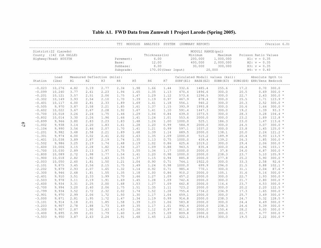
Table A1. FWD Data from Zumwalt 1 Project Laredo (Spring 2005). -------------------------------------------------------------------------------------------------------------------------------------- TTI MODULUS ANALYSIS SYSTEM (SUMMARY REPORT) (Version 6.0) -------------------------------------------------------------------------------------------------------------------------------------- District:22 (Laredo) MODULI RANGE(psi) County :142 (LA SALLE) Thickness(in) Minimum Maximum Poisson Ratio Values Highway/Road: H0035N Pavement: 6.00 200,000 1,000,000 H1: v = 0.35 Base: 12.00 400,000 2,000,000 H2: v = 0.35 Subbase: 8.00 30,000 300,000 H3: v = 0.35 Subgrade: 170.00(User Input) 20,000 H4: v = 0.40 -------------------------------------------------------------------------------------------------------------------------------------- Load Measured Deflection (mils): Calculated Moduli values (ksi): Absolute Dpth to Station (lbs) R1 R2 R3 R4 R5 R6 R7 SURF(E1) BASE(E2) SUBB(E3) SUBG(E4) ERR/Sens Bedrock -------------------------------------------------------------------------------------------------------------------------------------- -0.023 10,276 4.82 3.19 2.77 2.34 1.98 1.66 1.44 332.6 1485.4 255.6 17.2 0.70 300.0 -0.099 10,240 3.77 2.61 2.23 1.94 1.65 1.35 1.13 470.4 1896.6 300.0 20.5 0.69 300.0 * -0.201 10,121 3.57 2.51 2.06 1.75 1.47 1.29 1.12 573.6 1296.5 300.0 22.7 2.43 300.0 * -0.302 10,149 3.93 2.54 2.10 1.70 1.39 1.19 0.97 467.9 878.4 300.0 25.5 1.71 123.9 * -0.401 10,117 4.00 2.81 2.33 1.89 1.69 1.41 1.18 556.1 940.2 300.0 20.3 2.52 300.0 * -0.505 9,970 3.87 2.58 2.21 1.85 1.61 1.37 1.15 393.9 1993.8 300.0 20.6 1.64 300.0 * -0.602 10,022 3.67 2.67 2.28 1.92 1.67 1.41 1.10 591.4 1447.3 300.0 19.2 1.39 93.3 * -0.700 10,018 3.26 2.24 1.75 1.46 1.29 1.04 0.84 639.0 1073.5 300.0 28.3 3.28 104.4 * -0.802 10,014 3.30 2.26 1.96 1.66 1.41 1.24 1.01 553.6 2000.0 300.0 23.2 1.89 112.8 * -0.899 9,966 3.80 2.83 2.23 1.83 1.48 1.24 1.00 1000.0 525.1 186.3 23.0 1.47 113.6 * -1.002 9,938 3.14 2.20 1.83 1.61 1.28 1.20 0.99 584.9 2000.0 300.0 24.5 3.07 300.0 * -1.104 9,990 3.56 2.46 2.07 1.70 1.41 1.21 0.99 597.1 1037.2 300.0 23.8 1.45 125.0 * -1.201 9,982 3.48 2.58 2.21 1.89 1.68 1.39 1.14 689.5 2000.0 138.1 20.0 2.24 121.2 * -1.301 9,974 4.00 3.02 2.41 2.02 1.63 1.35 1.09 1000.0 515.2 189.9 20.4 0.93 113.5 * -1.401 10,038 3.89 2.87 2.19 1.74 1.35 1.13 0.75 1000.0 439.4 139.2 26.3 1.85 300.0 * -1.502 9,986 3.25 2.19 1.74 1.48 1.19 1.02 0.86 625.6 1019.2 300.0 29.4 2.06 300.0 * -1.600 10,006 3.15 2.28 1.82 1.54 1.27 1.09 0.88 943.5 835.4 300.0 26.4 1.96 103.1 * -1.700 10,030 2.89 2.13 1.97 1.75 1.55 1.34 1.17 1000.0 2000.0 37.8 24.0 6.87 300.0 * -1.800 10,089 2.72 1.98 1.77 1.54 1.41 1.20 0.98 1000.0 2000.0 238.3 23.7 5.10 105.9 * -1.900 10,018 2.82 1.92 1.63 1.55 1.37 1.15 0.94 885.8 2000.0 277.8 25.2 5.90 300.0 * -2.003 10,050 2.60 1.81 1.50 1.21 1.04 0.90 0.71 744.1 1922.0 300.0 33.3 2.58 92.6 * -2.101 9,875 3.45 2.56 2.15 1.75 1.49 1.24 0.98 1000.0 699.9 294.0 21.5 0.88 102.1 * -2.202 9,879 2.93 2.07 1.65 1.32 1.14 0.92 0.71 985.4 770.1 300.0 31.1 2.04 87.6 * -2.300 9,946 2.68 1.81 1.55 1.35 1.18 1.00 0.86 910.2 2000.0 105.1 31.6 5.16 300.0 * -2.401 9,910 3.51 2.33 1.99 1.70 1.46 1.27 1.09 457.2 2000.0 300.0 22.7 1.93 300.0 * -2.503 9,978 3.11 2.19 1.91 1.69 1.45 1.28 1.09 742.6 2000.0 300.0 21.7 2.80 300.0 * -2.600 9,934 3.31 2.25 2.00 1.68 1.53 1.27 1.09 662.8 2000.0 116.4 23.7 4.53 300.0 * -2.700 9,994 3.20 2.40 2.06 1.75 1.51 1.35 1.11 723.2 2000.0 300.0 20.2 2.20 122.5 * -2.799 9,934 3.52 2.72 2.32 2.02 1.74 1.52 1.28 755.4 1734.2 234.9 17.3 1.65 300.0 * -2.901 9,970 2.99 2.06 1.72 1.50 1.30 1.17 1.04 659.1 2000.0 300.0 25.7 3.49 300.0 * -3.000 9,871 2.81 1.95 1.72 1.47 1.34 1.19 0.99 914.8 2000.0 238.3 24.7 5.32 128.5 * -3.101 9,914 3.18 2.01 1.85 1.58 1.39 1.23 1.06 583.8 2000.0 300.0 24.4 4.49 300.0 * -3.203 9,907 2.78 1.88 1.73 1.49 1.35 1.17 1.01 992.4 2000.0 238.3 24.6 5.39 300.0 * -3.300 9,907 2.87 1.90 1.63 1.43 1.26 1.12 0.97 811.8 2000.0 150.4 28.2 6.00 300.0 * -3.400 9,895 2.99 2.01 1.79 1.60 1.40 1.25 1.09 809.8 2000.0 300.0 22.7 4.77 300.0 * -3.503 9,950 3.87 2.63 2.24 1.91 1.68 1.45 1.22 422.1 1954.0 300.0 19.5 2.22 300.0 *
67
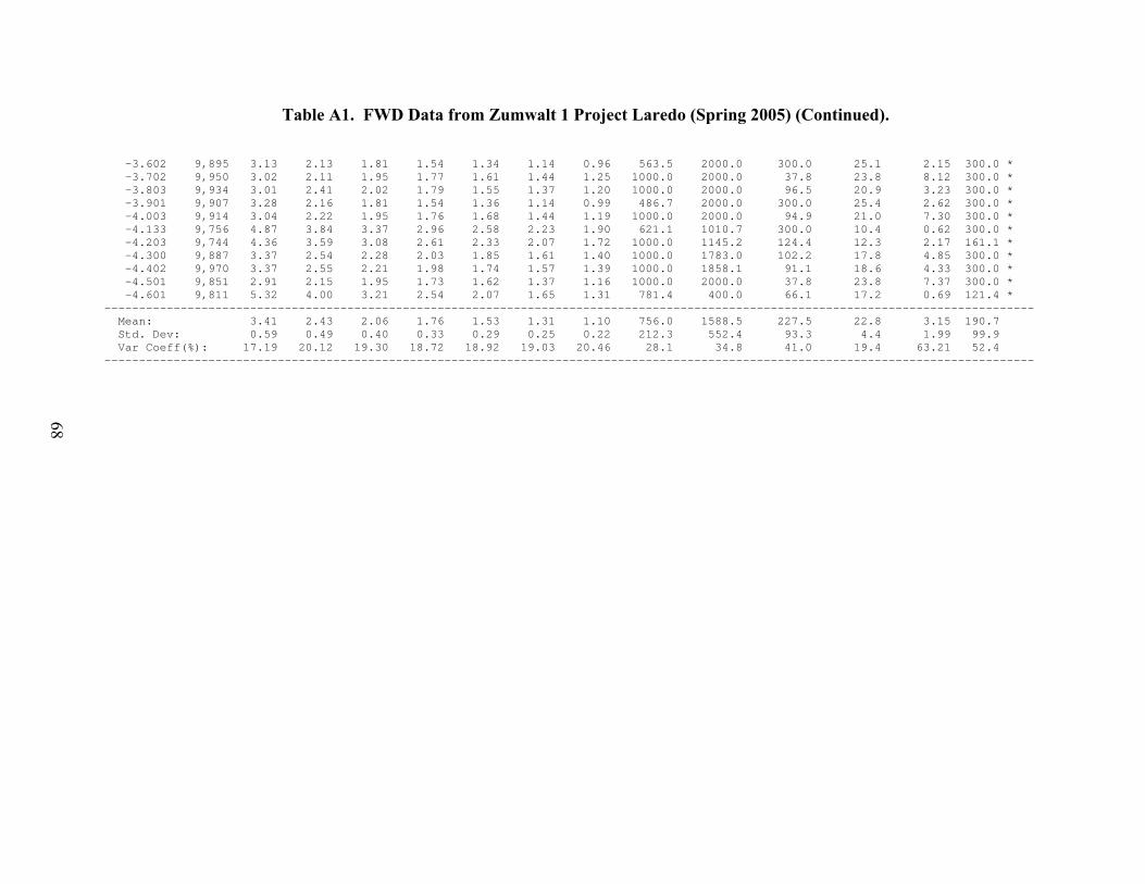
Table A1. FWD Data from Zumwalt 1 Project Laredo (Spring 2005) (Continued).
-3.602 9,895 3.13 2.13 1.81 1.54 1.34 1.14 0.96 563.5 2000.0 300.0 25.1 2.15 300.0 * -3.702 9,950 3.02 2.11 1.95 1.77 1.61 1.44 1.25 1000.0 2000.0 37.8 23.8 8.12 300.0 * -3.803 9,934 3.01 2.41 2.02 1.79 1.55 1.37 1.20 1000.0 2000.0 96.5 20.9 3.23 300.0 * -3.901 9,907 3.28 2.16 1.81 1.54 1.36 1.14 0.99 486.7 2000.0 300.0 25.4 2.62 300.0 * -4.003 9,914 3.04 2.22 1.95 1.76 1.68 1.44 1.19 1000.0 2000.0 94.9 21.0 7.30 300.0 * -4.133 9,756 4.87 3.84 3.37 2.96 2.58 2.23 1.90 621.1 1010.7 300.0 10.4 0.62 300.0 * -4.203 9,744 4.36 3.59 3.08 2.61 2.33 2.07 1.72 1000.0 1145.2 124.4 12.3 2.17 161.1 * -4.300 9,887 3.37 2.54 2.28 2.03 1.85 1.61 1.40 1000.0 1783.0 102.2 17.8 4.85 300.0 * -4.402 9,970 3.37 2.55 2.21 1.98 1.74 1.57 1.39 1000.0 1858.1 91.1 18.6 4.33 300.0 * -4.501 9,851 2.91 2.15 1.95 1.73 1.62 1.37 1.16 1000.0 2000.0 37.8 23.8 7.37 300.0 * -4.601 9,811 5.32 4.00 3.21 2.54 2.07 1.65 1.31 781.4 400.0 66.1 17.2 0.69 121.4 * -------------------------------------------------------------------------------------------------------------------------------------- Mean: 3.41 2.43 2.06 1.76 1.53 1.31 1.10 756.0 1588.5 227.5 22.8 3.15 190.7 Std. Dev: 0.59 0.49 0.40 0.33 0.29 0.25 0.22 212.3 552.4 93.3 4.4 1.99 99.9 Var Coeff(%): 17.19 20.12 19.30 18.72 18.92 19.03 20.46 28.1 34.8 41.0 19.4 63.21 52.4 --------------------------------------------------------------------------------------------------------------------------------------
68
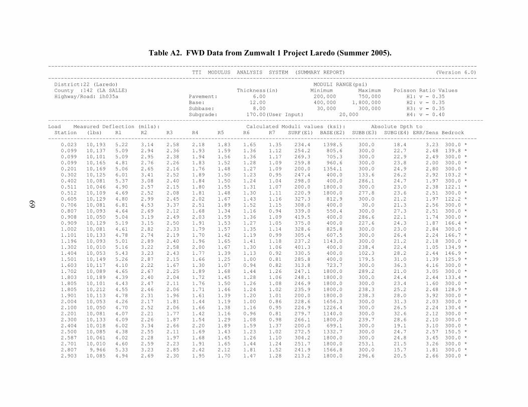
Table A2. FWD Data from Zumwalt 1 Project Laredo (Summer 2005). -------------------------------------------------------------------------------------------------------------------------------------- TTI MODULUS ANALYSIS SYSTEM (SUMMARY REPORT) (Version 6.0) -------------------------------------------------------------------------------------------------------------------------------------- District:22 (Laredo) MODULI RANGE(psi) County :142 (LA SALLE) Thickness(in) Minimum Maximum Poisson Ratio Values Highway/Road: ih035a Pavement: 6.00 200,000 750,000 H1: v = 0.35 Base: 12.00 400,000 1,800,000 H2: v = 0.35 Subbase: 8.00 30,000 300,000 H3: v = 0.35 Subgrade: 170.00(User Input) 20,000 H4: v = 0.40 ---------------------------------------------------------------------------------------------------------------------------------------- Load Measured Deflection (mils): Calculated Moduli values (ksi): Absolute Dpth to Station (lbs) R1 R2 R3 R4 R5 R6 R7 SURF(E1) BASE(E2) SUBB(E3) SUBG(E4) ERR/Sens Bedrock -------------------------------------------------------------------------------------------------------------------------------------- 0.023 10,193 5.22 3.14 2.58 2.18 1.83 1.65 1.35 234.4 1398.5 300.0 18.4 3.23 300.0 * 0.099 10,137 5.09 2.94 2.36 1.93 1.59 1.36 1.12 254.2 805.6 300.0 22.7 2.48 139.8 * 0.099 10,101 5.09 2.95 2.38 1.94 1.56 1.36 1.17 269.3 705.3 300.0 22.9 2.49 300.0 * 0.099 10,165 4.81 2.76 2.26 1.83 1.52 1.28 1.09 259.8 960.6 300.0 23.8 2.00 300.0 * 0.201 10,169 5.06 2.65 2.16 1.76 1.48 1.27 1.09 200.0 1354.1 300.0 24.9 2.80 300.0 * 0.302 10,125 6.01 3.41 2.52 1.89 1.50 1.23 0.95 247.4 400.0 133.6 26.2 2.92 103.2 * 0.402 10,081 5.37 3.08 2.40 1.84 1.50 1.24 1.04 298.0 400.0 286.1 24.7 1.97 300.0 * 0.511 10,046 4.90 2.57 2.15 1.80 1.55 1.31 1.07 200.0 1800.0 300.0 23.0 2.38 122.1 * 0.512 10,109 4.69 2.52 2.08 1.81 1.48 1.30 1.11 220.9 1800.0 277.8 23.6 2.51 300.0 * 0.605 10,129 4.80 2.99 2.45 2.02 1.67 1.43 1.16 327.3 812.9 300.0 21.2 1.97 122.2 * 0.706 10,081 6.81 4.53 3.37 2.51 1.89 1.52 1.15 308.0 400.0 30.0 21.3 2.56 300.0 * 0.807 10,093 4.64 2.69 2.12 1.68 1.34 1.16 0.94 339.0 550.4 300.0 27.3 2.51 300.0 * 0.908 10,050 5.04 3.19 2.49 2.03 1.59 1.36 1.09 419.5 400.0 286.6 22.1 1.74 300.0 * 0.909 10,129 5.19 3.15 2.50 1.91 1.53 1.27 1.05 375.0 400.0 227.6 24.3 1.87 166.4 * 1.002 10,081 4.61 2.82 2.33 1.79 1.57 1.35 1.14 328.6 825.8 300.0 23.0 2.84 300.0 * 1.101 10,133 4.78 2.74 2.19 1.70 1.42 1.19 0.99 305.4 607.5 300.0 26.4 2.24 166.7 * 1.196 10,093 5.01 2.89 2.40 1.96 1.65 1.41 1.18 237.2 1143.0 300.0 21.2 2.18 300.0 * 1.302 10,010 5.16 3.22 2.58 2.00 1.67 1.30 1.06 401.3 400.0 238.4 22.4 1.05 134.9 * 1.404 10,053 5.43 3.23 2.43 1.77 1.39 1.13 0.92 330.5 400.0 102.3 28.2 2.44 146.9 * 1.501 10,149 5.26 2.87 2.15 1.66 1.25 1.00 0.81 285.8 400.0 179.5 31.0 1.39 125.9 * 1.603 10,117 4.10 2.22 1.67 1.30 1.07 0.94 0.82 313.8 723.7 300.0 36.3 4.16 300.0 * 1.702 10,089 4.65 2.67 2.25 1.89 1.68 1.44 1.26 247.1 1800.0 289.2 21.0 3.05 300.0 * 1.803 10,189 4.39 2.40 2.04 1.72 1.45 1.28 1.06 248.1 1800.0 300.0 24.4 2.44 133.4 * 1.805 10,101 4.43 2.47 2.11 1.76 1.50 1.26 1.08 246.9 1800.0 300.0 23.4 1.60 300.0 * 1.805 10,212 4.55 2.46 2.06 1.71 1.46 1.24 1.02 235.9 1800.0 238.3 25.2 2.48 128.9 * 1.901 10,113 4.78 2.31 1.96 1.61 1.39 1.20 1.01 200.0 1800.0 238.3 28.0 3.92 300.0 * 2.004 10,053 4.26 2.17 1.81 1.44 1.19 1.00 0.86 228.6 1656.3 300.0 31.3 2.03 300.0 * 2.100 10,050 4.70 2.52 2.06 1.66 1.38 1.16 0.95 224.9 1226.4 300.0 26.5 2.24 130.4 * 2.201 10,081 4.07 2.21 1.77 1.42 1.16 0.96 0.81 279.7 1140.0 300.0 32.6 2.12 300.0 * 2.300 10,133 4.09 2.26 1.87 1.54 1.29 1.08 0.98 266.1 1800.0 239.7 28.6 2.10 300.0 * 2.404 10,018 6.02 3.34 2.66 2.20 1.89 1.59 1.37 200.0 699.1 300.0 19.1 3.10 300.0 * 2.500 10,085 4.38 2.55 2.11 1.69 1.43 1.23 1.02 272.5 1332.7 300.0 24.7 2.57 150.5 * 2.587 10,061 4.02 2.28 1.97 1.68 1.45 1.26 1.10 304.2 1800.0 300.0 24.8 3.45 300.0 * 2.701 10,010 4.60 2.59 2.23 1.91 1.65 1.44 1.24 251.7 1800.0 253.1 21.5 3.26 300.0 * 2.807 9,966 5.33 3.23 2.85 2.42 2.12 1.81 1.52 241.9 1566.8 300.0 15.7 1.81 300.0 * 2.903 10,085 4.94 2.69 2.30 1.95 1.70 1.47 1.28 213.2 1800.0 296.6 20.5 2.66 300.0 *
69
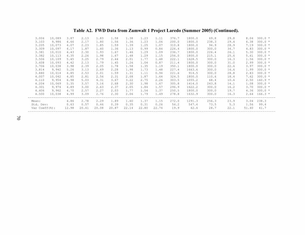
Table A2. FWD Data from Zumwalt 1 Project Laredo (Summer 2005) (Continued). 3.004 10,089 3.87 2.13 1.83 1.58 1.38 1.23 1.11 376.7 1800.0 69.8 29.8 8.04 300.0 * 3.103 9,986 4.66 2.17 1.80 1.56 1.36 1.23 1.06 200.0 1800.0 238.3 29.4 6.38 300.0 * 3.205 10,073 4.07 2.23 1.85 1.59 1.39 1.25 1.07 310.8 1800.0 94.9 28.9 7.19 300.0 * 3.309 10,097 4.17 1.87 1.60 1.36 1.13 0.99 0.84 226.4 1800.0 300.0 34.7 4.83 300.0 * 3.381 10,010 4.43 2.30 1.93 1.67 1.46 1.29 1.09 236.7 1800.0 226.4 26.1 5.30 300.0 * 3.382 10,113 4.35 2.26 1.98 1.67 1.48 1.29 1.15 256.0 1800.0 215.1 25.6 5.61 300.0 * 3.506 10,109 5.45 3.25 2.79 2.44 2.01 1.77 1.48 222.1 1628.5 300.0 16.3 1.56 300.0 * 3.608 10,093 4.42 2.13 1.79 1.45 1.26 1.04 0.87 211.4 1800.0 300.0 31.0 2.99 300.0 * 3.706 10,038 3.98 2.39 2.05 1.78 1.58 1.35 1.19 350.1 1800.0 300.0 22.6 3.97 300.0 * 3.814 9,942 5.26 3.13 2.69 2.28 1.98 1.73 1.48 227.4 1663.6 300.0 16.6 1.99 300.0 * 3.880 10,014 4.85 2.53 2.01 1.59 1.31 1.11 0.94 221.6 914.5 300.0 28.8 2.83 300.0 * 4.007 10,042 4.85 2.81 2.56 2.31 2.08 1.87 1.64 324.5 1800.0 110.6 18.4 7.62 300.0 * 4.110 9,954 6.98 5.03 4.31 3.67 3.22 2.75 2.26 303.5 1055.2 68.4 10.6 2.50 160.9 * 4.204 10,069 5.35 3.57 3.16 2.68 2.30 1.98 1.67 305.8 1414.0 243.8 14.1 1.08 300.0 * 4.301 9,974 4.89 3.00 2.63 2.37 2.05 1.84 1.57 296.9 1622.2 300.0 16.2 3.70 300.0 * 4.406 9,962 4.70 2.57 2.27 2.03 1.77 1.54 1.37 250.5 1800.0 300.0 19.7 4.36 300.0 * 4.500 10,038 4.99 3.09 2.76 2.30 2.06 1.79 1.49 278.8 1632.9 300.0 16.3 2.64 166.3 * -------------------------------------------------------------------------------------------------------------------------------------- Mean: 4.86 2.78 2.29 1.89 1.60 1.37 1.15 272.0 1291.3 256.3 23.9 3.04 238.3 Std. Dev: 0.63 0.57 0.46 0.39 0.35 0.31 0.26 54.2 547.4 73.5 5.3 1.56 99.4 Var Coeff(%): 12.98 20.41 20.08 20.87 22.14 22.80 22.74 19.9 42.4 28.7 22.1 51.40 41.7 --------------------------------------------------------------------------------------------------------------------------------------
70
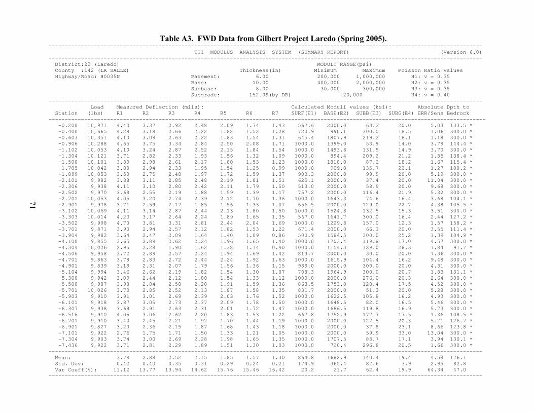
Table A3. FWD Data from Gilbert Project Laredo (Spring 2005). -------------------------------------------------------------------------------------------------------------------------------------- TTI MODULUS ANALYSIS SYSTEM (SUMMARY REPORT) (Version 6.0) -------------------------------------------------------------------------------------------------------------------------------------- District:22 (Laredo) MODULI RANGE(psi) County :142 (LA SALLE) Thickness(in) Minimum Maximum Poisson Ratio Values Highway/Road: H0035N Pavement: 6.00 200,000 1,000,000 H1: v = 0.35 Base: 10.00 400,000 2,000,000 H2: v = 0.35 Subbase: 8.00 30,000 300,000 H3: v = 0.35 Subgrade: 152.09(by DB) 20,000 H4: v = 0.40 -------------------------------------------------------------------------------------------------------------------------------------- Load Measured Deflection (mils): Calculated Moduli values (ksi): Absolute Dpth to Station (lbs) R1 R2 R3 R4 R5 R6 R7 SURF(E1) BASE(E2) SUBB(E3) SUBG(E4) ERR/Sens Bedrock --------------------------------------------------------------------------------------------------------------------------------------- -0.200 10,971 4.40 3.37 2.92 2.48 2.09 1.74 1.43 567.6 2000.0 63.2 20.0 5.03 133.5 * -0.400 10,665 4.28 3.18 2.66 2.22 1.82 1.52 1.28 720.9 990.1 300.0 18.5 1.06 300.0 * -0.603 10,351 4.10 3.09 2.63 2.22 1.83 1.54 1.31 645.4 1807.9 219.2 18.1 1.18 300.0 * -0.906 10,288 4.65 3.75 3.34 2.84 2.50 2.08 1.71 1000.0 1399.0 53.9 14.0 3.79 144.4 * -1.102 10,053 4.10 3.24 2.87 2.52 2.15 1.84 1.54 1000.0 1493.8 131.9 14.9 3.70 300.0 * -1.304 10,121 3.71 2.82 2.33 1.93 1.56 1.32 1.09 1000.0 894.4 209.2 21.2 1.85 138.4 * -1.500 10,101 3.80 2.98 2.61 2.17 1.80 1.53 1.23 1000.0 1818.0 87.2 18.2 1.67 115.4 * -1.705 10,042 3.80 2.94 2.33 1.95 1.54 1.25 0.99 1000.0 909.0 135.7 22.1 1.27 100.2 * -1.899 10,053 3.50 2.75 2.48 1.97 1.72 1.59 1.37 900.3 2000.0 99.9 20.0 5.19 300.0 * -2.101 9,982 3.88 3.11 2.85 2.48 2.19 1.81 1.51 625.1 2000.0 37.4 20.0 11.04 300.0 * -2.306 9,938 4.11 3.10 2.80 2.42 2.11 1.79 1.50 513.0 2000.0 58.9 20.0 9.68 300.0 * -2.502 9,970 3.69 2.55 2.19 1.88 1.59 1.39 1.17 757.2 2000.0 116.4 21.9 5.32 300.0 * -2.701 10,053 4.05 3.20 2.74 2.39 2.12 1.70 1.36 1000.0 1643.3 74.6 16.4 3.68 104.1 * -2.901 9,978 3.71 2.59 2.17 1.85 1.56 1.33 1.07 656.5 2000.0 129.0 22.7 4.38 105.5 * -3.102 10,069 4.11 3.14 2.87 2.44 2.13 1.80 1.50 1000.0 1524.8 132.5 15.3 3.51 300.0 * -3.303 10,014 4.23 3.17 2.64 2.24 1.89 1.65 1.35 567.0 1641.7 300.0 16.4 2.44 127.2 * -3.502 9,998 4.70 3.81 3.31 2.81 2.44 2.04 1.69 1000.0 1229.8 157.0 12.3 1.57 158.2 * -3.701 9,871 3.90 2.94 2.57 2.12 1.82 1.53 1.22 671.4 2000.0 66.3 20.0 3.55 111.4 * -3.904 9,982 3.64 2.47 2.09 1.64 1.40 1.09 0.86 500.9 1584.5 300.0 25.2 1.39 104.9 * -4.100 9,855 3.65 2.89 2.62 2.24 1.96 1.65 1.40 1000.0 1703.4 119.8 17.0 4.57 300.0 * -4.304 10,026 2.95 2.28 1.90 1.62 1.38 1.14 0.90 1000.0 1154.3 129.0 28.3 7.84 91.7 * -4.506 9,958 3.72 2.89 2.57 2.24 1.94 1.69 1.42 813.7 2000.0 30.0 20.0 7.36 300.0 * -4.701 9,863 3.78 2.83 2.72 2.44 2.24 1.92 1.63 1000.0 1615.9 104.4 16.2 9.48 300.0 * -4.901 9,839 3.19 2.31 2.07 1.79 1.56 1.36 1.15 989.0 2000.0 300.0 20.0 4.31 300.0 * -5.104 9,994 3.46 2.62 2.19 1.82 1.54 1.30 1.07 708.3 1964.9 300.0 20.7 1.83 131.1 * -5.300 9,942 3.09 2.44 2.12 1.80 1.54 1.33 1.12 1000.0 2000.0 276.0 20.3 2.64 300.0 * -5.500 9,907 3.98 2.84 2.58 2.20 1.91 1.59 1.36 863.5 1753.0 120.4 17.5 4.52 300.0 * -5.701 10,026 3.70 2.85 2.52 2.13 1.87 1.58 1.35 831.7 2000.0 51.3 20.0 5.28 300.0 * -5.903 9,910 3.91 3.01 2.69 2.39 2.03 1.76 1.52 1000.0 1622.5 105.8 16.2 4.93 300.0 * -6.101 9,918 3.87 3.05 2.73 2.37 2.09 1.78 1.50 1000.0 1648.5 82.0 16.5 5.46 300.0 * -6.307 9,938 3.69 2.91 2.63 2.31 2.01 1.72 1.47 1000.0 1686.5 119.8 16.9 5.73 300.0 * -6.516 9,910 4.05 3.06 2.62 2.20 1.83 1.53 1.22 667.8 1752.9 177.7 17.5 1.36 108.5 * -6.701 9,910 3.40 2.45 2.21 1.92 1.70 1.44 1.19 1000.0 2000.0 122.5 20.3 5.71 126.7 * -6.901 9,827 3.20 2.36 2.15 1.87 1.68 1.43 1.18 1000.0 2000.0 37.8 23.1 8.66 123.8 * -7.101 9,922 2.76 1.75 1.71 1.50 1.33 1.21 1.05 1000.0 2000.0 59.9 33.0 13.04 300.0 * -7.304 9,903 3.74 3.00 2.69 2.28 1.98 1.65 1.35 1000.0 1707.5 88.7 17.1 3.94 130.1 * -7.436 9,922 3.71 2.81 2.29 1.89 1.51 1.30 1.03 1000.0 720.4 296.8 20.5 1.66 300.0 * -------------------------------------------------------------------------------------------------------------------------------------- Mean: 3.79 2.88 2.52 2.15 1.85 1.57 1.30 864.8 1682.9 140.4 19.4 4.58 176.1 Std. Dev: 0.42 0.40 0.35 0.31 0.29 0.24 0.21 174.9 365.4 87.6 3.9 2.95 82.8 Var Coeff(%): 11.12 13.77 13.94 14.62 15.76 15.46 16.42 20.2 21.7 62.4 19.9 64.34 47.0 --------------------------------------------------------------------------------------------------------------------------------------
71
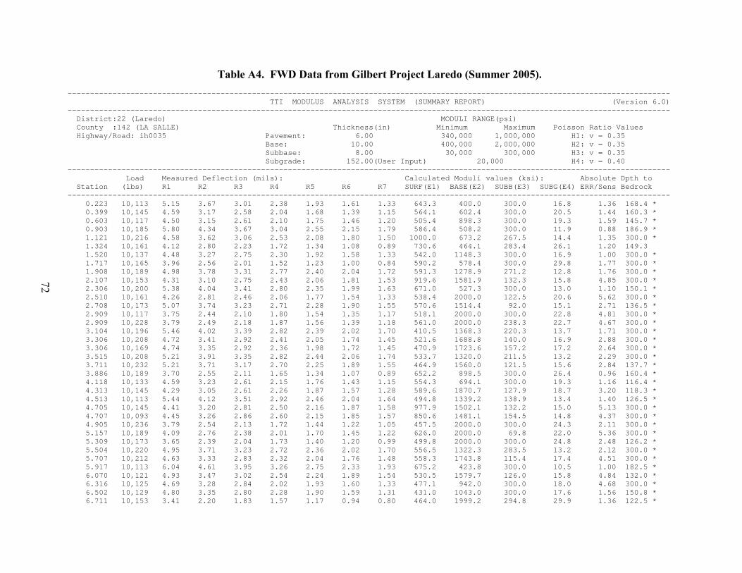
Table A4. FWD Data from Gilbert Project Laredo (Summer 2005). -------------------------------------------------------------------------------------------------------------------------------------- TTI MODULUS ANALYSIS SYSTEM (SUMMARY REPORT) (Version 6.0) -------------------------------------------------------------------------------------------------------------------------------------- District:22 (Laredo) MODULI RANGE(psi) County :142 (LA SALLE) Thickness(in) Minimum Maximum Poisson Ratio Values Highway/Road: ih0035 Pavement: 6.00 340,000 1,000,000 H1: v = 0.35 Base: 10.00 400,000 2,000,000 H2: v = 0.35 Subbase: 8.00 30,000 300,000 H3: v = 0.35 Subgrade: 152.00(User Input) 20,000 H4: v = 0.40 -------------------------------------------------------------------------------------------------------------------------------------- Load Measured Deflection (mils): Calculated Moduli values (ksi): Absolute Dpth to Station (lbs) R1 R2 R3 R4 R5 R6 R7 SURF(E1) BASE(E2) SUBB(E3) SUBG(E4) ERR/Sens Bedrock -------------------------------------------------------------------------------------------------------------------------------------- 0.223 10,113 5.15 3.67 3.01 2.38 1.93 1.61 1.33 643.3 400.0 300.0 16.8 1.36 168.4 * 0.399 10,145 4.59 3.17 2.58 2.04 1.68 1.39 1.15 564.1 602.4 300.0 20.5 1.44 160.3 * 0.603 10,117 4.50 3.15 2.61 2.10 1.75 1.46 1.20 505.4 898.3 300.0 19.3 1.59 145.7 * 0.903 10,185 5.80 4.34 3.67 3.04 2.55 2.15 1.79 586.4 508.2 300.0 11.9 0.88 186.9 * 1.121 10,216 4.58 3.62 3.06 2.53 2.08 1.80 1.50 1000.0 673.2 267.5 14.4 1.35 300.0 * 1.324 10,161 4.12 2.80 2.23 1.72 1.34 1.08 0.89 730.6 464.1 283.4 26.1 1.20 149.3 1.520 10,137 4.48 3.27 2.75 2.30 1.92 1.58 1.33 542.0 1148.3 300.0 16.9 1.00 300.0 * 1.717 10,165 3.96 2.56 2.01 1.52 1.23 1.00 0.84 590.2 578.4 300.0 29.8 1.77 300.0 * 1.908 10,189 4.98 3.78 3.31 2.77 2.40 2.04 1.72 591.3 1278.9 271.2 12.8 1.76 300.0 * 2.107 10,153 4.31 3.10 2.75 2.43 2.06 1.81 1.53 919.6 1581.9 132.3 15.8 4.85 300.0 * 2.306 10,200 5.38 4.04 3.41 2.80 2.35 1.99 1.63 671.0 527.3 300.0 13.0 1.10 150.1 * 2.510 10,161 4.26 2.81 2.46 2.06 1.77 1.54 1.33 538.4 2000.0 122.5 20.6 5.62 300.0 * 2.708 10,173 5.07 3.74 3.23 2.71 2.28 1.90 1.55 570.6 1514.4 92.0 15.1 2.71 136.5 * 2.909 10,117 3.75 2.44 2.10 1.80 1.54 1.35 1.17 518.1 2000.0 300.0 22.8 4.81 300.0 * 2.909 10,228 3.79 2.49 2.18 1.87 1.56 1.39 1.18 561.0 2000.0 238.3 22.7 4.67 300.0 * 3.104 10,196 5.46 4.02 3.39 2.82 2.39 2.02 1.70 410.5 1368.3 220.3 13.7 1.71 300.0 * 3.306 10,208 4.72 3.41 2.92 2.41 2.05 1.74 1.45 521.6 1688.8 140.0 16.9 2.88 300.0 * 3.306 10,169 4.74 3.35 2.92 2.36 1.98 1.72 1.45 470.9 1723.6 157.2 17.2 2.64 300.0 * 3.515 10,208 5.21 3.91 3.35 2.82 2.44 2.06 1.74 533.7 1320.0 211.5 13.2 2.29 300.0 * 3.711 10,232 5.21 3.71 3.17 2.70 2.25 1.89 1.55 464.9 1560.0 121.5 15.6 2.84 137.7 * 3.886 10,189 3.70 2.55 2.11 1.65 1.34 1.07 0.89 652.2 898.5 300.0 26.4 0.96 160.4 * 4.118 10,133 4.59 3.23 2.61 2.15 1.76 1.43 1.15 554.3 694.1 300.0 19.3 1.16 116.4 * 4.313 10,145 4.29 3.05 2.61 2.26 1.87 1.57 1.28 589.6 1870.7 127.9 18.7 3.20 118.3 * 4.513 10,113 5.44 4.12 3.51 2.92 2.46 2.04 1.64 494.8 1339.2 138.9 13.4 1.40 126.5 * 4.705 10,145 4.41 3.20 2.81 2.50 2.16 1.87 1.58 977.9 1502.1 132.2 15.0 5.13 300.0 * 4.707 10,093 4.45 3.26 2.86 2.60 2.15 1.85 1.57 850.6 1481.1 154.5 14.8 4.37 300.0 * 4.905 10,236 3.79 2.54 2.13 1.72 1.44 1.22 1.05 457.5 2000.0 300.0 24.3 2.11 300.0 * 5.157 10,189 4.09 2.76 2.38 2.01 1.70 1.45 1.22 626.0 2000.0 69.8 22.0 5.36 300.0 * 5.309 10,173 3.65 2.39 2.04 1.73 1.40 1.20 0.99 499.8 2000.0 300.0 24.8 2.48 126.2 * 5.504 10,220 4.95 3.71 3.23 2.72 2.36 2.02 1.70 556.5 1322.3 283.5 13.2 2.12 300.0 * 5.707 10,212 4.63 3.33 2.83 2.32 2.04 1.76 1.48 558.3 1743.8 115.4 17.4 4.51 300.0 * 5.917 10,113 6.04 4.61 3.95 3.26 2.75 2.33 1.93 675.2 423.8 300.0 10.5 1.00 182.5 * 6.070 10,121 4.93 3.47 3.02 2.54 2.24 1.89 1.54 530.5 1579.7 126.0 15.8 4.84 132.0 * 6.316 10,125 4.69 3.28 2.84 2.02 1.93 1.60 1.33 477.1 942.0 300.0 18.0 4.68 300.0 * 6.502 10,129 4.80 3.35 2.80 2.28 1.90 1.59 1.31 431.0 1043.0 300.0 17.6 1.56 150.8 * 6.711 10,153 3.41 2.20 1.83 1.57 1.17 0.94 0.80 464.0 1999.2 294.8 29.9 1.36 122.5 *
72
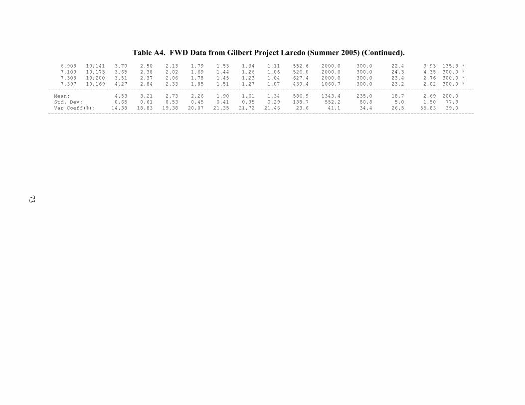
Table A4. FWD Data from Gilbert Project Laredo (Summer 2005) (Continued). 6.908 10,141 3.70 2.50 2.13 1.79 1.53 1.34 1.11 552.6 2000.0 300.0 22.4 3.93 135.8 * 7.109 10,173 3.65 2.38 2.02 1.69 1.44 1.26 1.06 526.0 2000.0 300.0 24.3 4.35 300.0 * 7.308 10,200 3.51 2.37 2.06 1.78 1.45 1.23 1.04 627.4 2000.0 300.0 23.4 2.76 300.0 * 7.397 10,169 4.27 2.84 2.33 1.85 1.51 1.27 1.07 439.4 1060.7 300.0 23.2 2.02 300.0 * -------------------------------------------------------------------------------------------------------------------------------------- Mean: 4.53 3.21 2.73 2.26 1.90 1.61 1.34 586.9 1343.4 235.0 18.7 2.69 200.0 Std. Dev: 0.65 0.61 0.53 0.45 0.41 0.35 0.29 138.7 552.2 80.8 5.0 1.50 77.9 Var Coeff(%): 14.38 18.83 19.38 20.07 21.35 21.72 21.46 23.6 41.1 34.4 26.5 55.83 39.0 --------------------------------------------------------------------------------------------------------------------------------------
73
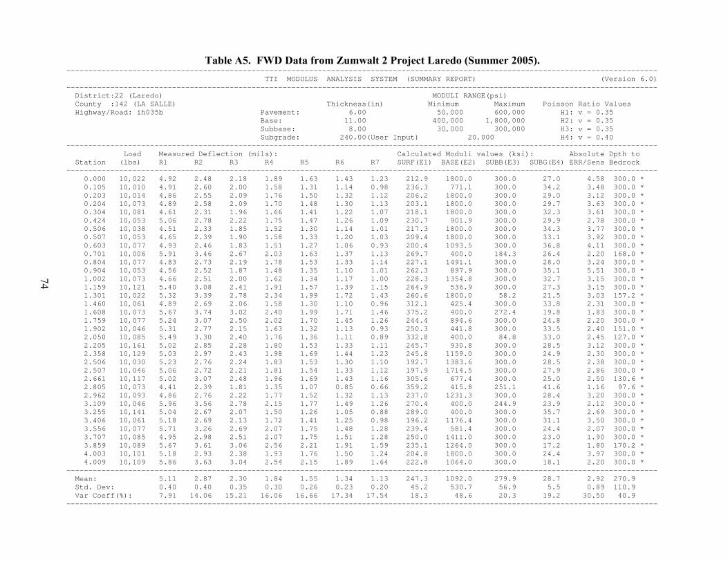
Table A5. FWD Data from Zumwalt 2 Project Laredo (Summer 2005). -------------------------------------------------------------------------------------------------------------------------------------- TTI MODULUS ANALYSIS SYSTEM (SUMMARY REPORT) (Version 6.0) -------------------------------------------------------------------------------------------------------------------------------------- District:22 (Laredo) MODULI RANGE(psi) County :142 (LA SALLE) Thickness(in) Minimum Maximum Poisson Ratio Values Highway/Road: ih035b Pavement: 6.00 50,000 600,000 H1: v = 0.35 Base: 11.00 400,000 1,800,000 H2: v = 0.35 Subbase: 8.00 30,000 300,000 H3: v = 0.35 Subgrade: 240.00(User Input) 20,000 H4: v = 0.40 -------------------------------------------------------------------------------------------------------------------------------------- Load Measured Deflection (mils): Calculated Moduli values (ksi): Absolute Dpth to Station (lbs) R1 R2 R3 R4 R5 R6 R7 SURF(E1) BASE(E2) SUBB(E3) SUBG(E4) ERR/Sens Bedrock -------------------------------------------------------------------------------------------------------------------------------------- 0.000 10,022 4.92 2.48 2.18 1.89 1.63 1.43 1.23 212.9 1800.0 300.0 27.0 4.58 300.0 * 0.105 10,010 4.91 2.60 2.00 1.58 1.31 1.14 0.98 236.3 771.1 300.0 34.2 3.48 300.0 * 0.203 10,014 4.86 2.55 2.09 1.76 1.50 1.32 1.12 206.2 1800.0 300.0 29.0 3.12 300.0 * 0.204 10,073 4.89 2.58 2.09 1.70 1.48 1.30 1.13 203.1 1800.0 300.0 29.7 3.63 300.0 * 0.304 10,081 4.61 2.31 1.96 1.66 1.41 1.22 1.07 218.1 1800.0 300.0 32.3 3.61 300.0 * 0.424 10,053 5.06 2.78 2.22 1.75 1.47 1.26 1.09 230.7 901.9 300.0 29.9 2.78 300.0 * 0.506 10,038 4.51 2.33 1.85 1.52 1.30 1.14 1.01 217.3 1800.0 300.0 34.3 3.77 300.0 * 0.507 10,053 4.65 2.39 1.90 1.58 1.33 1.20 1.03 209.4 1800.0 300.0 33.1 3.92 300.0 * 0.603 10,077 4.93 2.46 1.83 1.51 1.27 1.06 0.93 200.4 1093.5 300.0 36.8 4.11 300.0 * 0.701 10,006 5.91 3.46 2.67 2.03 1.63 1.37 1.13 269.7 400.0 184.3 26.4 2.20 168.0 * 0.804 10,077 4.83 2.73 2.19 1.78 1.53 1.33 1.14 227.1 1491.1 300.0 28.0 3.24 300.0 * 0.904 10,053 4.56 2.52 1.87 1.48 1.35 1.10 1.01 262.3 897.9 300.0 35.1 5.51 300.0 * 1.002 10,073 4.66 2.51 2.00 1.62 1.34 1.17 1.00 228.3 1354.8 300.0 32.7 3.15 300.0 * 1.159 10,121 5.40 3.08 2.41 1.91 1.57 1.39 1.15 264.9 536.9 300.0 27.3 3.15 300.0 * 1.301 10,022 5.32 3.39 2.78 2.34 1.99 1.72 1.43 260.6 1800.0 58.2 21.5 3.03 157.2 * 1.460 10,061 4.89 2.69 2.06 1.58 1.30 1.10 0.96 312.1 425.4 300.0 33.8 2.31 300.0 * 1.608 10,073 5.67 3.74 3.02 2.40 1.99 1.71 1.46 375.2 400.0 272.4 19.8 1.83 300.0 * 1.759 10,077 5.24 3.07 2.50 2.02 1.70 1.45 1.26 244.4 894.6 300.0 24.8 2.20 300.0 * 1.902 10,046 5.31 2.77 2.15 1.63 1.32 1.13 0.93 250.3 441.8 300.0 33.5 2.40 151.0 * 2.050 10,085 5.49 3.30 2.40 1.76 1.36 1.11 0.89 332.8 400.0 84.8 33.0 2.45 127.0 * 2.205 10,161 5.02 2.85 2.28 1.80 1.53 1.33 1.11 245.7 930.8 300.0 28.5 3.12 300.0 * 2.358 10,129 5.03 2.97 2.43 1.98 1.69 1.44 1.23 245.8 1159.0 300.0 24.9 2.30 300.0 * 2.506 10,030 5.23 2.76 2.24 1.83 1.53 1.30 1.10 192.7 1383.6 300.0 28.5 2.38 300.0 * 2.507 10,046 5.06 2.72 2.21 1.81 1.54 1.33 1.12 197.9 1714.5 300.0 27.9 2.86 300.0 * 2.661 10,117 5.02 3.07 2.48 1.96 1.69 1.43 1.16 305.6 677.4 300.0 25.0 2.50 130.6 * 2.805 10,073 4.41 2.39 1.81 1.35 1.07 0.85 0.66 359.2 415.8 251.1 41.6 1.16 97.6 * 2.962 10,093 4.86 2.76 2.22 1.77 1.52 1.32 1.13 237.0 1231.3 300.0 28.4 3.20 300.0 * 3.109 10,046 5.96 3.56 2.78 2.15 1.77 1.49 1.26 270.4 400.0 244.9 23.9 2.12 300.0 * 3.255 10,141 5.04 2.67 2.07 1.50 1.26 1.05 0.88 289.0 400.0 300.0 35.7 2.69 300.0 * 3.406 10,061 5.18 2.69 2.13 1.72 1.41 1.25 0.98 196.2 1176.4 300.0 31.1 3.50 300.0 * 3.556 10,077 5.71 3.26 2.69 2.07 1.75 1.48 1.28 239.4 581.4 300.0 24.4 2.07 300.0 * 3.707 10,085 4.95 2.98 2.51 2.07 1.75 1.51 1.28 250.0 1411.0 300.0 23.0 1.90 300.0 * 3.859 10,089 5.67 3.61 3.06 2.56 2.21 1.91 1.59 235.1 1264.0 300.0 17.2 1.80 170.2 * 4.003 10,101 5.18 2.93 2.38 1.93 1.76 1.50 1.24 204.8 1800.0 300.0 24.4 3.97 300.0 * 4.009 10,109 5.86 3.63 3.04 2.54 2.15 1.89 1.64 222.8 1064.0 300.0 18.1 2.20 300.0 * -------------------------------------------------------------------------------------------------------------------------------------- Mean: 5.11 2.87 2.30 1.84 1.55 1.34 1.13 247.3 1092.0 279.9 28.7 2.92 270.9 Std. Dev: 0.40 0.40 0.35 0.30 0.26 0.23 0.20 45.2 530.7 56.9 5.5 0.89 110.9 Var Coeff(%): 7.91 14.06 15.21 16.06 16.66 17.34 17.54 18.3 48.6 20.3 19.2 30.50 40.9 --------------------------------------------------------------------------------------------------------------------------------------
74
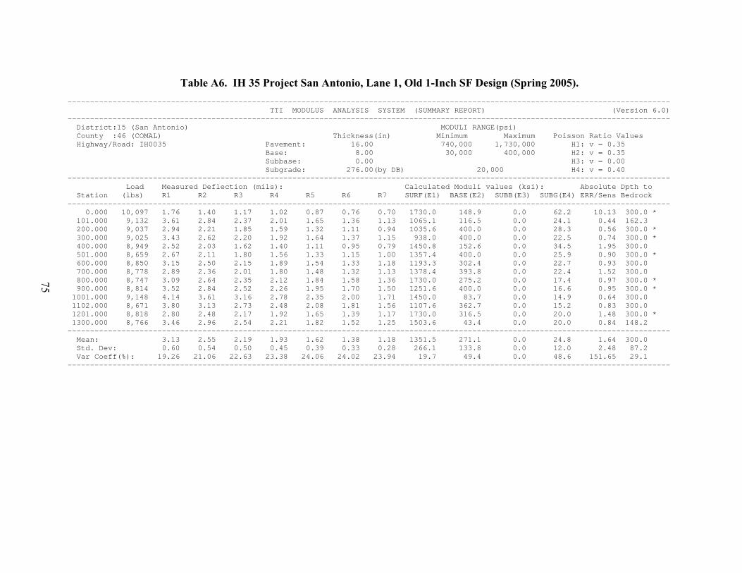
Table A6. IH 35 Project San Antonio, Lane 1, Old 1-Inch SF Design (Spring 2005). -------------------------------------------------------------------------------------------------------------------------------------- TTI MODULUS ANALYSIS SYSTEM (SUMMARY REPORT) (Version 6.0) -------------------------------------------------------------------------------------------------------------------------------------- District:15 (San Antonio) MODULI RANGE(psi) County :46 (COMAL) Thickness(in) Minimum Maximum Poisson Ratio Values Highway/Road: IH0035 Pavement: 16.00 740,000 1,730,000 H1: v = 0.35 Base: 8.00 30,000 400,000 H2: v = 0.35 Subbase: 0.00 H3: v = 0.00 Subgrade: 276.00(by DB) 20,000 H4: v = 0.40 -------------------------------------------------------------------------------------------------------------------------------------- Load Measured Deflection (mils): Calculated Moduli values (ksi): Absolute Dpth to Station (lbs) R1 R2 R3 R4 R5 R6 R7 SURF(E1) BASE(E2) SUBB(E3) SUBG(E4) ERR/Sens Bedrock -------------------------------------------------------------------------------------------------------------------------------------- 0.000 10,097 1.76 1.40 1.17 1.02 0.87 0.76 0.70 1730.0 148.9 0.0 62.2 10.13 300.0 * 101.000 9,132 3.61 2.84 2.37 2.01 1.65 1.36 1.13 1065.1 116.5 0.0 24.1 0.44 162.3 200.000 9,037 2.94 2.21 1.85 1.59 1.32 1.11 0.94 1035.6 400.0 0.0 28.3 0.56 300.0 * 300.000 9,025 3.43 2.62 2.20 1.92 1.64 1.37 1.15 938.0 400.0 0.0 22.5 0.74 300.0 * 400.000 8,949 2.52 2.03 1.62 1.40 1.11 0.95 0.79 1450.8 152.6 0.0 34.5 1.95 300.0 501.000 8,659 2.67 2.11 1.80 1.56 1.33 1.15 1.00 1357.4 400.0 0.0 25.9 0.90 300.0 * 600.000 8,850 3.15 2.50 2.15 1.89 1.54 1.33 1.18 1193.3 302.4 0.0 22.7 0.93 300.0 700.000 8,778 2.89 2.36 2.01 1.80 1.48 1.32 1.13 1378.4 393.8 0.0 22.4 1.52 300.0 800.000 8,747 3.09 2.64 2.35 2.12 1.84 1.58 1.36 1730.0 275.2 0.0 17.4 0.97 300.0 * 900.000 8,814 3.52 2.84 2.52 2.26 1.95 1.70 1.50 1251.6 400.0 0.0 16.6 0.95 300.0 * 1001.000 9,148 4.14 3.61 3.16 2.78 2.35 2.00 1.71 1450.0 83.7 0.0 14.9 0.64 300.0 1102.000 8,671 3.80 3.13 2.73 2.48 2.08 1.81 1.56 1107.6 362.7 0.0 15.2 0.83 300.0 1201.000 8,818 2.80 2.48 2.17 1.92 1.65 1.39 1.17 1730.0 316.5 0.0 20.0 1.48 300.0 * 1300.000 8,766 3.46 2.96 2.54 2.21 1.82 1.52 1.25 1503.6 43.4 0.0 20.0 0.84 148.2 -------------------------------------------------------------------------------------------------------------------------------------- Mean: 3.13 2.55 2.19 1.93 1.62 1.38 1.18 1351.5 271.1 0.0 24.8 1.64 300.0 Std. Dev: 0.60 0.54 0.50 0.45 0.39 0.33 0.28 266.1 133.8 0.0 12.0 2.48 87.2 Var Coeff(%): 19.26 21.06 22.63 23.38 24.06 24.02 23.94 19.7 49.4 0.0 48.6 151.65 29.1 --------------------------------------------------------------------------------------------------------------------------------------
75
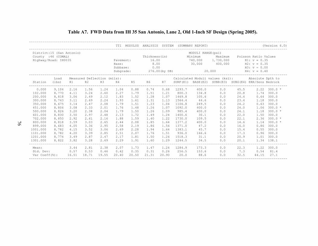
Table A7. FWD Data from IH 35 San Antonio, Lane 2, Old 1-Inch SF Design (Spring 2005). -------------------------------------------------------------------------------------------------------------------------------------- TTI MODULUS ANALYSIS SYSTEM (SUMMARY REPORT) (Version 6.0) -------------------------------------------------------------------------------------------------------------------------------------- District:15 (San Antonio) MODULI RANGE(psi) County :46 (COMAL) Thickness(in) Minimum Maximum Poisson Ratio Values Highway/Road: IH0035 Pavement: 16.00 740,000 1,730,000 H1: v = 0.35 Base: 8.00 30,000 400,000 H2: v = 0.35 Subbase: 0.00 H3: v = 0.00 Subgrade: 276.00(by DB) 20,000 H4: v = 0.40 -------------------------------------------------------------------------------------------------------------------------------------- Load Measured Deflection (mils): Calculated Moduli values (ksi): Absolute Dpth to Station (lbs) R1 R2 R3 R4 R5 R6 R7 SURF(E1) BASE(E2) SUBB(E3) SUBG(E4) ERR/Sens Bedrock -------------------------------------------------------------------------------------------------------------------------------------- 0.000 9,104 2.16 1.56 1.24 1.04 0.88 0.74 0.68 1293.7 400.0 0.0 45.5 2.22 300.0 * 102.000 8,770 4.11 3.24 2.60 2.27 1.79 1.51 1.21 800.3 134.8 0.0 20.8 1.74 300.0 200.000 8,818 3.06 2.49 2.12 1.83 1.52 1.28 1.07 1469.8 105.6 0.0 24.4 0.64 300.0 300.000 8,743 3.11 2.69 2.24 1.93 1.61 1.31 1.13 1564.4 44.6 0.0 23.4 1.18 300.0 350.000 8,675 3.14 2.47 2.08 1.79 1.51 1.23 1.04 1106.8 249.5 0.0 24.2 0.63 300.0 451.000 8,806 3.08 2.33 2.01 1.76 1.48 1.26 1.07 1092.0 400.0 0.0 24.0 1.06 300.0 * 500.000 8,826 3.20 2.38 2.04 1.79 1.50 1.26 1.09 985.4 400.0 0.0 24.1 1.18 300.0 * 601.000 8,830 3.50 2.97 2.48 2.13 1.72 1.49 1.24 1400.6 30.1 0.0 22.0 1.50 300.0 702.000 8,850 2.92 2.61 2.16 1.88 1.59 1.40 1.22 1730.0 109.5 0.0 22.1 2.36 300.0 * 800.000 8,818 3.59 3.03 2.65 2.44 2.08 1.85 1.64 1377.2 400.0 0.0 14.6 1.14 300.0 * 899.000 8,683 4.05 3.36 2.95 2.58 2.19 1.86 1.56 1371.0 47.2 0.0 16.0 0.86 300.0 1001.000 8,782 4.15 3.52 3.06 2.69 2.28 1.94 1.64 1383.1 45.7 0.0 15.4 0.55 300.0 1101.000 8,782 4.20 3.39 2.85 2.51 2.07 1.76 1.51 936.0 166.6 0.0 17.3 0.96 300.0 1201.000 8,774 3.49 2.87 2.47 2.17 1.81 1.50 1.26 1518.3 31.1 0.0 20.9 1.01 300.0 1301.000 8,822 3.82 3.28 2.69 2.29 1.91 1.60 1.29 1244.5 34.5 0.0 20.1 1.34 138.1 -------------------------------------------------------------------------------------------------------------------------------------- Mean: 3.44 2.81 2.38 2.07 1.73 1.47 1.24 1284.9 173.3 0.0 22.3 1.22 300.0 Std. Dev: 0.57 0.53 0.46 0.42 0.35 0.31 0.26 256.5 153.6 0.0 7.3 0.54 81.4 Var Coeff(%): 16.51 18.71 19.55 20.40 20.50 21.31 20.90 20.0 88.6 0.0 32.5 44.15 27.1 --------------------------------------------------------------------------------------------------------------------------------------
76
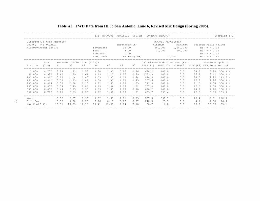
Table A8. FWD Data from IH 35 San Antonio, Lane 6, Revised Mix Design (Spring 2005). -------------------------------------------------------------------------------------------------------------------------------------- TTI MODULUS ANALYSIS SYSTEM (SUMMARY REPORT) (Version 6.0) -------------------------------------------------------------------------------------------------------------------------------------- District:15 (San Antonio) MODULI RANGE(psi) County :46 (COMAL) Thickness(in) Minimum Maximum Poisson Ratio Values Highway/Road: IH0035 Pavement: 16.00 600,000 1,480,000 H1: v = 0.35 Base: 8.00 30,000 400,000 H2: v = 0.35 Subbase: 0.00 H3: v = 0.00 Subgrade: 194.86(by DB) 20,000 H4: v = 0.40 -------------------------------------------------------------------------------------------------------------------------------------- Load Measured Deflection (mils): Calculated Moduli values (ksi): Absolute Dpth to Station (lbs) R1 R2 R3 R4 R5 R6 R7 SURF(E1) BASE(E2) SUBB(E3) SUBG(E4) ERR/Sens Bedrock -------------------------------------------------------------------------------------------------------------------------------------- 0.000 8,770 3.24 1.83 1.55 1.30 1.00 0.95 0.86 624.2 400.0 0.0 34.6 5.98 300.0 * 49.000 8,929 2.62 1.89 1.61 1.43 1.20 1.06 0.89 1363.3 400.0 0.0 26.9 3.42 300.0 * 100.000 8,810 3.10 2.14 1.83 1.59 1.33 1.13 0.94 944.5 400.0 0.0 24.6 2.95 143.7 * 150.000 8,842 3.30 2.25 1.87 1.58 1.33 1.09 0.95 757.6 400.0 0.0 25.3 2.26 300.0 * 200.000 8,814 3.50 2.50 2.10 1.82 1.50 1.23 1.05 771.8 400.0 0.0 21.6 1.34 300.0 * 250.000 8,830 3.54 2.49 2.06 1.75 1.46 1.18 1.02 707.4 400.0 0.0 22.6 1.08 300.0 * 300.000 8,806 3.44 2.35 1.95 1.63 1.35 1.09 0.90 690.2 400.0 0.0 24.8 1.16 150.6 * 352.000 8,782 3.85 2.69 2.20 1.82 1.49 1.18 1.01 603.7 333.6 0.0 22.6 0.33 159.0 -------------------------------------------------------------------------------------------------------------------------------------- Mean: 3.32 2.27 1.90 1.62 1.33 1.11 0.95 807.8 391.7 0.0 25.4 2.31 218.9 Std. Dev: 0.36 0.30 0.23 0.18 0.17 0.09 0.07 248.0 23.5 0.0 4.1 1.80 76.8 Var Coeff(%): 10.91 13.33 12.13 11.41 12.61 7.84 7.18 30.7 6.0 0.0 16.2 78.03 35.1 --------------------------------------------------------------------------------------------------------------------------------------
77
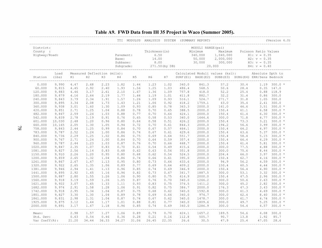
Table A9. FWD Data from IH 35 Project in Waco (Summer 2005). -------------------------------------------------------------------------------------------------------------------------------------- TTI MODULUS ANALYSIS SYSTEM (SUMMARY REPORT) (Version 6.0) -------------------------------------------------------------------------------------------------------------------------------------- District: MODULI RANGE(psi) County : Thickness(in) Minimum Maximum Poisson Ratio Values Highway/Road: Pavement: 6.50 340,000 1,040,000 H1: v = 0.35 Base: 14.00 50,000 2,000,000 H2: v = 0.35 Subbase: 8.00 30,000 300,000 H3: v = 0.35 Subgrade: 271.50(by DB) 20,000 H4: v = 0.40 -------------------------------------------------------------------------------------------------------------------------------------- Load Measured Deflection (mils): Calculated Moduli values (ksi): Absolute Dpth to Station (lbs) R1 R2 R3 R4 R5 R6 R7 SURF(E1) BASE(E2) SUBB(E3) SUBG(E4) ERR/Sens Bedrock -------------------------------------------------------------------------------------------------------------------------------------- 0.000 9,990 4.47 2.68 2.23 1.82 1.44 1.23 1.02 340.0 841.3 57.2 30.4 1.19 300.0 * 60.000 9,815 4.45 2.92 2.40 1.93 1.56 1.25 1.03 486.4 568.5 50.6 28.4 0.35 147.0 120.000 9,883 4.46 3.17 2.61 2.10 1.67 1.36 1.09 757.8 418.0 52.2 25.4 0.88 118.9 180.000 9,879 4.16 2.64 2.19 1.77 1.44 1.19 1.01 411.8 882.7 32.2 31.4 0.86 300.0 240.000 9,843 3.79 2.34 1.91 1.57 1.26 1.09 0.93 516.1 524.7 271.7 31.8 1.05 300.0 300.000 9,895 3.34 2.08 1.73 1.43 1.21 1.06 0.92 418.2 1759.1 43.0 35.4 2.41 300.0 360.000 9,938 3.01 1.60 1.30 1.09 0.93 0.85 0.78 363.3 2000.0 161.0 46.6 3.51 300.0 * 420.000 9,851 2.71 1.25 1.04 0.88 0.78 0.70 0.65 388.5 2000.0 150.4 61.1 6.58 300.0 * 482.000 9,847 2.59 1.24 1.03 0.88 0.77 0.70 0.64 424.1 2000.0 150.4 61.4 6.30 300.0 * 542.000 9,839 2.78 1.19 0.91 0.76 0.65 0.58 0.53 340.0 1644.6 300.0 71.8 4.77 300.0 * 601.000 10,030 2.48 1.20 0.96 0.80 0.64 0.58 0.51 426.2 2000.0 150.4 73.3 3.21 300.0 * 660.000 10,165 2.05 1.30 1.05 0.94 0.72 0.70 0.61 844.3 2000.0 194.2 56.6 3.99 300.0 * 758.000 9,843 2.44 1.25 0.99 0.84 0.70 0.67 0.57 464.1 2000.0 150.4 64.2 4.97 300.0 * 783.000 9,787 2.52 1.24 1.00 0.86 0.74 0.67 0.61 429.6 2000.0 150.4 63.6 5.37 300.0 * 840.000 9,736 2.29 1.25 1.02 0.86 0.75 0.69 0.64 551.7 2000.0 150.4 58.4 5.15 300.0 * 900.000 9,767 2.71 1.24 1.00 0.84 0.70 0.64 0.59 357.4 2000.0 150.4 66.4 4.29 300.0 * 960.000 9,787 2.44 1.23 1.03 0.87 0.76 0.70 0.66 468.7 2000.0 150.4 61.4 5.81 300.0 * 1020.000 9,847 2.35 1.07 0.83 0.70 0.61 0.54 0.49 415.6 2000.0 300.0 77.5 4.88 300.0 * 1081.000 9,827 2.56 1.14 0.83 0.68 0.62 0.63 0.56 351.8 2000.0 300.0 75.6 8.44 300.0 * 1150.000 9,910 2.26 1.20 0.95 0.80 0.68 0.62 0.54 524.5 2000.0 204.4 66.0 3.97 300.0 * 1200.000 9,859 2.65 1.32 1.04 0.86 0.74 0.66 0.61 395.0 2000.0 150.4 62.7 4.16 300.0 * 1261.000 9,867 2.67 1.47 1.13 0.95 0.80 0.73 0.66 433.6 2000.0 94.9 56.2 4.59 300.0 * 1320.000 9,922 2.65 1.35 1.06 0.89 0.77 0.69 0.64 409.2 2000.0 150.4 60.5 4.44 300.0 * 1381.000 9,946 2.94 1.41 1.13 0.96 0.85 0.74 0.69 346.9 2000.0 150.4 56.4 4.90 300.0 * 1441.000 9,895 2.92 1.45 1.16 0.96 0.82 0.73 0.67 341.7 1887.5 300.0 53.1 3.32 300.0 * 1500.000 9,887 2.80 1.55 1.26 1.06 0.90 0.80 0.75 414.9 2000.0 150.4 47.5 2.96 300.0 * 1560.000 9,918 3.19 1.59 1.26 1.05 0.87 0.76 0.70 340.0 1266.2 300.0 50.6 2.63 300.0 * 1621.000 9,922 3.07 1.65 1.33 1.11 0.93 0.83 0.75 374.5 1411.2 300.0 45.2 2.82 300.0 * 1682.000 9,974 2.91 1.58 1.28 1.06 0.91 0.82 0.75 384.7 2000.0 176.3 47.3 3.43 300.0 * 1742.000 9,918 2.95 1.34 1.04 0.87 0.75 0.68 0.62 340.0 1592.8 300.0 61.3 4.69 300.0 * 1801.000 9,827 3.30 1.30 1.04 0.89 0.78 0.69 0.66 340.0 974.7 300.0 62.4 8.40 300.0 * 1861.000 9,831 2.98 1.31 1.04 0.87 0.74 0.67 0.62 340.0 1478.7 300.0 61.7 4.74 300.0 * 1925.000 9,875 3.12 1.44 1.17 1.01 0.88 0.81 0.77 340.0 1809.6 300.0 49.7 5.25 300.0 * 2000.000 9,891 3.17 1.47 1.18 0.96 0.85 0.74 0.69 340.0 1286.9 300.0 54.4 4.57 300.0 * -------------------------------------------------------------------------------------------------------------------------------------- Mean: 2.98 1.57 1.27 1.06 0.89 0.79 0.70 424.1 1657.2 189.5 54.6 4.08 300.0 Std. Dev: 0.63 0.54 0.46 0.36 0.28 0.21 0.16 112.8 505.7 90.7 13.8 1.92 85.7 Var Coeff(%): 21.20 34.44 36.33 34.27 31.06 26.45 22.35 26.6 30.5 47.9 25.4 47.05 28.6 --------------------------------------------------------------------------------------------------------------------------------------
78
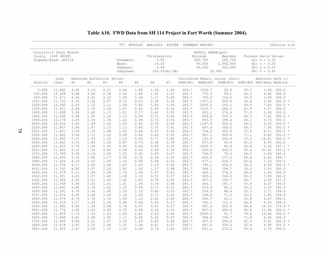
Table A10. FWD Data from SH 114 Project in Fort Worth (Summer 2004). ------------------------------------------------------------------------------------------------------------------------------------- TTI MODULUS ANALYSIS SYSTEM (SUMMARY REPORT) (Version 6.0) -------------------------------------------------------------------------------------------------------------------------------------- District:2 (Fort Worth) MODULI RANGE(psi) County :249 (WISE) Thickness(in) Minimum Maximum Poisson Ratio Values Highway/Road: sh0114 Pavement: 2.50 283,700 283,700 H1: v = 0.35 Base: 16.00 50,000 2,000,000 H2: v = 0.35 Subbase: 8.00 30,000 300,000 H3: v = 0.35 Subgrade: 250.09(by DB) 20,000 H4: v = 0.40 -------------------------------------------------------------------------------------------------------------------------------------- Load Measured Deflection (mils): Calculated Moduli values (ksi): Absolute Dpth to Station (lbs) R1 R2 R3 R4 R5 R6 R7 SURF(E1) BASE(E2) SUBB(E3) SUBG(E4) ERR/Sens Bedrock -------------------------------------------------------------------------------------------------------------------------------------- 0.000 11,662 4.30 3.15 2.21 2.06 1.68 1.28 1.00 283.7 1056.7 90.8 30.3 3.94 300.0 100.000 10,308 4.68 3.46 2.38 2.32 1.86 1.42 1.07 283.7 773.3 93.1 24.3 4.82 300.0 200.000 11,571 4.54 2.91 2.10 1.93 1.46 1.11 0.85 283.7 703.0 152.2 36.0 3.08 300.0 1001.000 11,722 2.33 1.32 0.87 0.72 0.53 0.38 0.28 283.7 1507.2 300.0 94.6 5.96 300.0 * 1200.000 12,350 2.54 1.72 1.11 1.04 0.82 0.65 0.56 283.7 2000.0 105.1 69.9 7.45 300.0 * 1300.000 11,921 2.94 1.78 1.26 1.07 0.83 0.65 0.54 283.7 1225.7 285.0 63.9 3.07 300.0 1400.000 11,698 3.04 1.80 1.13 1.01 0.77 0.60 0.50 283.7 923.1 276.6 71.3 5.18 300.0 1800.000 11,448 3.58 1.95 1.15 1.13 0.89 0.71 0.60 283.7 629.8 300.0 64.5 7.42 300.0 * 1900.000 12,179 3.49 2.25 1.36 1.22 0.98 0.73 0.56 283.7 893.5 199.4 60.1 5.74 300.0 2000.000 12,024 3.00 1.69 1.02 1.05 0.81 0.75 0.59 283.7 1187.9 300.0 68.6 9.35 300.0 * 2100.000 11,857 3.49 1.87 1.13 1.13 0.85 0.70 0.61 283.7 687.4 300.0 68.7 7.56 300.0 * 2201.000 11,821 3.29 1.78 1.08 1.03 0.86 0.67 0.56 283.7 754.2 300.0 71.9 8.11 300.0 * 2300.000 11,682 3.06 1.71 1.10 0.99 0.82 0.63 0.59 283.7 921.1 300.0 71.1 5.82 300.0 * 2400.000 11,642 7.27 1.93 1.25 1.15 0.93 0.71 0.60 283.7 163.4 300.0 72.5 14.61 300.0 * 2500.000 11,662 3.10 1.83 1.00 0.87 0.73 0.48 0.39 283.7 837.9 92.9 91.5 8.00 300.0 2600.000 11,623 2.79 1.59 1.05 0.85 0.63 0.45 0.35 283.7 1093.3 92.6 92.6 3.35 267.1 * 3001.000 11,666 3.52 1.32 0.85 0.58 0.42 0.28 0.18 283.7 653.0 300.0 94.6 31.42 165.2 * 3703.000 11,789 3.78 2.16 1.49 1.22 0.92 0.65 0.47 283.7 766.5 70.3 66.2 2.69 246.4 3800.000 11,650 3.55 1.82 1.17 0.92 0.72 0.54 0.40 283.7 629.5 137.2 84.6 2.62 284.7 3900.000 11,666 4.19 2.02 1.50 1.10 0.90 0.68 0.52 283.7 477.1 254.7 65.4 1.10 300.0 4000.000 11,754 4.17 2.69 1.92 1.67 1.43 1.19 0.90 283.7 790.1 300.0 36.3 4.56 300.0 * 4101.000 11,762 4.85 3.07 2.16 1.83 1.50 1.17 0.98 283.7 566.1 196.7 36.5 3.03 300.0 4200.000 11,579 5.11 2.89 1.99 1.72 1.36 1.07 0.83 283.7 400.3 274.5 40.0 2.45 300.0 4302.000 11,591 4.03 2.37 1.45 1.38 1.10 0.72 0.57 283.7 629.2 164.5 55.2 7.09 300.0 4302.000 11,583 4.24 2.41 1.69 1.42 1.03 0.78 0.56 283.7 607.2 100.7 54.7 2.34 237.5 4304.000 11,758 4.58 2.43 1.61 1.41 1.06 0.76 0.68 283.7 460.1 191.7 55.9 4.27 300.0 4400.000 11,642 3.95 2.36 1.42 1.25 0.95 0.71 0.53 283.7 633.4 90.3 63.3 5.23 300.0 4500.000 11,591 4.70 2.64 1.80 1.50 1.15 0.80 0.55 283.7 504.9 86.4 52.3 3.71 198.4 4701.000 11,674 4.35 2.48 1.58 1.28 1.00 0.71 0.54 283.7 548.6 71.3 62.5 3.85 254.8 4900.000 11,579 4.73 2.78 1.76 1.49 1.13 0.81 0.59 283.7 505.7 63.1 53.8 4.27 300.0 5000.000 11,519 3.17 1.63 1.05 0.88 0.66 0.43 0.27 283.7 760.1 111.2 94.6 6.03 300.0 5400.000 11,960 3.96 1.44 0.96 0.78 0.57 0.41 0.27 283.7 451.6 300.0 94.6 10.14 174.9 * 5501.000 11,778 3.00 1.43 0.84 0.72 0.58 0.36 0.35 283.7 847.2 300.0 94.6 11.08 300.0 * 5600.000 11,829 1.76 1.93 1.23 1.00 0.81 0.63 0.44 283.7 2000.0 91.7 78.4 19.86 300.0 * 5604.000 11,698 3.81 2.05 1.22 1.11 0.82 0.62 0.47 283.7 568.8 194.7 71.9 5.06 300.0 5701.000 11,654 4.66 2.41 1.47 1.35 1.09 0.85 0.69 283.7 407.3 300.0 55.3 5.61 300.0 * 5800.000 11,619 3.85 2.25 1.48 1.31 1.06 0.81 0.67 283.7 641.5 300.0 52.9 4.08 300.0 * 5901.000 11,929 3.47 2.06 1.37 1.20 0.94 0.73 0.65 283.7 831.1 272.2 59.6 3.78 300.0
79
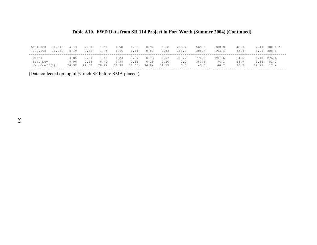
Table A10. FWD Data from SH 114 Project in Fort Worth (Summer 2004) (Continued). 6601.000 11,543 4.13 2.50 1.51 1.50 1.08 0.94 0.60 283.7 565.0 300.0 48.3 7.47 300.0 * 7000.000 11,734 5.19 2.80 1.75 1.46 1.11 0.81 0.55 283.7 388.4 103.3 55.4 3.94 300.0 -------------------------------------------------------------------------------------------------------------------------------------- Mean: 3.85 2.17 1.41 1.24 0.97 0.73 0.57 283.7 774.8 201.6 64.5 6.48 276.6 Std. Dev: 0.96 0.53 0.40 0.38 0.31 0.25 0.20 0.0 383.6 94.1 18.9 5.36 51.2 Var Coeff(%): 24.92 24.53 28.24 30.33 31.65 34.04 34.57 0.0 49.5 46.7 29.3 82.71 17.4 --------------------------------------------------------------------------------------------------------------------------------------
(Data collected on top of ¾-inch SF before SMA placed.)
80