Sect

ion

: Sy

stem

Ove

rvie

w

1

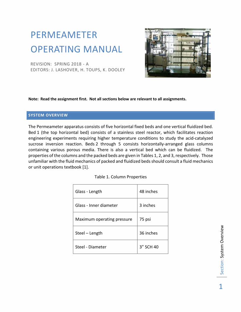
PERMEAMETER

OPERATING MANUAL

REVISION: SPRING 2018 - A EDITORS: J. LASHOVER, H. TOUPS, K. DOOLEY

Note: Read the assignment first. Not all sections below are relevant to all assignments.

SYSTEM OVERVIEW

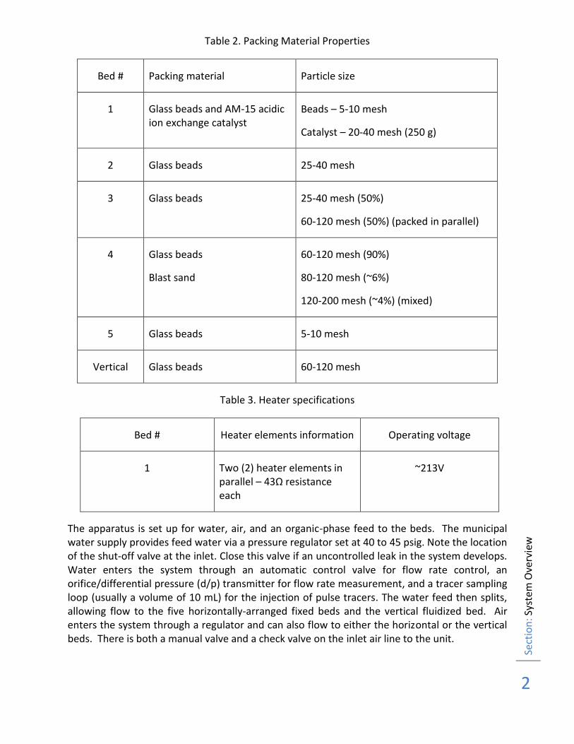
The Permeameter apparatus consists of five horizontal fixed beds and one vertical fluidized bed. Bed 1 (the top horizontal bed) consists of a stainless steel reactor, which facilitates reaction engineering experiments requiring higher temperature conditions to study the acid-catalyzed sucrose inversion reaction. Beds 2 through 5 consists horizontally-arranged glass columns containing various porous media. There is also a vertical bed which can be fluidized. The properties of the columns and the packed beds are given in Tables 1, 2, and 3, respectively. Those unfamiliar with the fluid mechanics of packed and fluidized beds should consult a fluid mechanics or unit operations textbook [1].

Table 1. Column Properties

Glass - Length 48 inches

Glass - Inner diameter 3 inches

Maximum operating pressure 75 psi

Steel – Length 36 inches

Steel - Diameter 3” SCH 40

Sect

ion

: Sy

stem

Ove

rvie

w

2

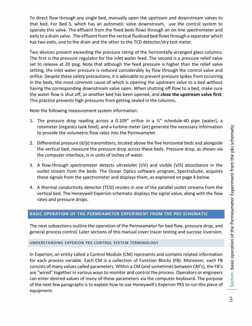
Table 2. Packing Material Properties

Bed # Packing material Particle size

1 Glass beads and AM-15 acidic ion exchange catalyst

Beads – 5-10 mesh

Catalyst – 20-40 mesh (250 g)

2 Glass beads 25-40 mesh

3 Glass beads 25-40 mesh (50%)

60-120 mesh (50%) (packed in parallel)

4 Glass beads

Blast sand

60-120 mesh (90%)

80-120 mesh (~6%)

120-200 mesh (~4%) (mixed)

5 Glass beads 5-10 mesh

Vertical Glass beads 60-120 mesh

Table 3. Heater specifications

Bed # Heater elements information Operating voltage

1 Two (2) heater elements in parallel – 43Ω resistance each

~213V

The apparatus is set up for water, air, and an organic-phase feed to the beds. The municipal water supply provides feed water via a pressure regulator set at 40 to 45 psig. Note the location of the shut-off valve at the inlet. Close this valve if an uncontrolled leak in the system develops. Water enters the system through an automatic control valve for flow rate control, an orifice/differential pressure (d/p) transmitter for flow rate measurement, and a tracer sampling loop (usually a volume of 10 mL) for the injection of pulse tracers. The water feed then splits, allowing flow to the five horizontally-arranged fixed beds and the vertical fluidized bed. Air enters the system through a regulator and can also flow to either the horizontal or the vertical beds. There is both a manual valve and a check valve on the inlet air line to the unit.

Sect

ion

: b

asic

op

erat

ion

of

the

Pe

rmea

met

er E

xper

imen

t fr

om

th

e p

ks s

chem

atic

3

To direct flow through any single bed, manually open the upstream and downstream valves to that bed. For Bed 5, which has an automatic valve downstream, use the control system to operate this valve. The effluent from the fixed beds flows through an on-line spectrometer and exits to a drain valve. The effluent from the vertical fluidized bed flows through a separator which has two exits, one to the drain and the other to the TCD detector/dry test meter.

Two devices prevent exceeding the pressure rating of the horizontally-arranged glass columns. The first is the pressure regulator for the inlet water feed. The second is a pressure relief valve set to release at 20 psig. Note that although the feed pressure is higher than the relief valve setting, the inlet water pressure is reduced considerably by flow through the control valve and orifice. Despite these safety precautions, it is advisable to prevent pressure spikes from occurring in the beds, the most common cause of which is opening the upstream valve to a bed without having the corresponding downstream valve open. When shutting off flow to a bed, make sure the water flow is shut off, or another bed has been opened, and close the upstream valve first. This practice prevents high pressures from getting sealed in the columns.

Note the following measurement system information:

1. The pressure drop reading across a 0.109” orifice in a ½” schedule-40 pipe (water), a rotameter (organics tank feed), and a turbine meter (air) generate the necessary information to provide the volumetric flow rates into the Permeameter.

2. Differential pressure (d/p) transmitters, located above the five horizontal beds and alongside the vertical bed, measure the pressure drop across these beds. Pressure drop, as shown via the computer interface, is in units of inches of water.

3. A flow-through spectrometer detects ultraviolet (UV) and visible (VIS) absorbance in the outlet stream from the beds. The Ocean Optics software program, SpectraSuite, acquires these signals from the spectrometer and displays them, as explained on page 4 below.

4. A thermal conductivity detector (TCD) resides in one of the parallel outlet streams from the vertical bed. The Honeywell Experion schematic displays the signal value, along with the flow rates and pressure drops.

BASIC OPERATION OF THE PERMEAMETER EXPERIMENT FROM THE PKS SCHEMATIC

The next subsections outline the operation of the Permeameter for bed flow, pressure drop, and general process control. Later sections of this manual cover tracer testing and sucrose inversion.

UNDERSTANDING EXPERION PKS CONTROL SYSTE M TERMINOLOGY

In Experion, an entity called a Control Module (CM) represents and contains related information for each process variable. Each CM is a collection of Function Blocks (FB). Moreover, each FB consists of many values called parameters. Within a CM (and sometimes between CM’s), the FB’s are “wired” together in various ways to monitor and control the process. Operators or engineers can enter desired values of many of these parameters via the computer keyboard. The purpose of the next few paragraphs is to explain how to use Honeywell’s Experion PKS to run this piece of equipment.

Sect

ion

: b

asic

op

erat

ion

of

the

Pe

rmea

met

er E

xper

imen

t fr

om

th

e p

ks s

chem

atic

4

LOGGING INTO HONEYWELL

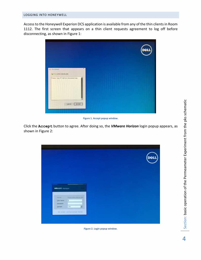
Access to the Honeywell Experion DCS application is available from any of the thin clients in Room 1112. The first screen that appears on a thin client requests agreement to log off before disconnecting, as shown in Figure 1:

Figure 1. Accept popup window.

Click the Accept button to agree. After doing so, the VMware Horizon login popup appears, as shown in Figure 2:

Figure 2. Login popup window.

Sect

ion

: b

asic

op

erat

ion

of

the

Pe

rmea

met

er E

xper

imen

t fr

om

th

e p

ks s

chem

atic

5

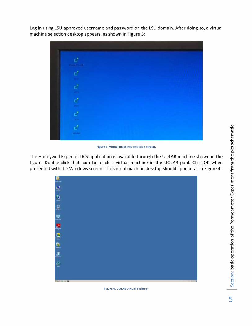
Log in using LSU-approved username and password on the LSU domain. After doing so, a virtual machine selection desktop appears, as shown in Figure 3:

Figure 3. Virtual machines selection screen.

The Honeywell Experion DCS application is available through the UOLAB machine shown in the figure. Double-click that icon to reach a virtual machine in the UOLAB pool. Click OK when presented with the Windows screen. The virtual machine desktop should appear, as in Figure 4:

Figure 4. UOLAB virtual desktop.

Sect

ion

: b

asic

op

erat

ion

of

the

Pe

rmea

met

er E

xper

imen

t fr

om

th

e p

ks s

chem

atic

6

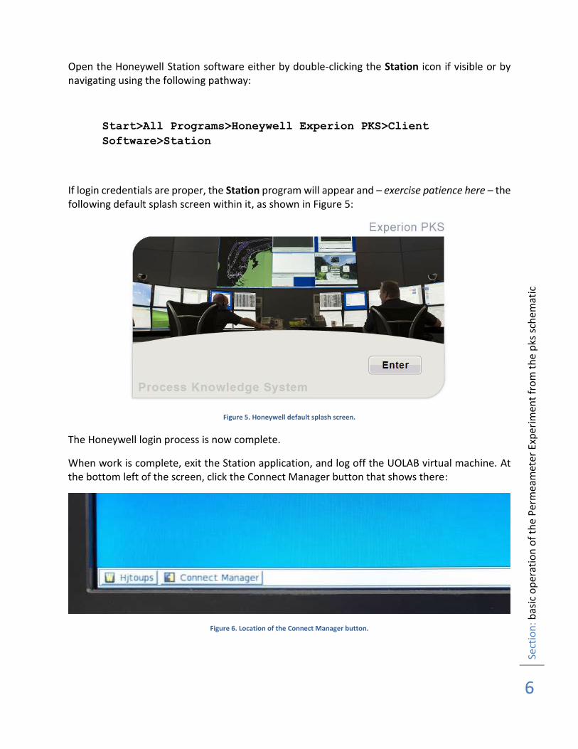
Open the Honeywell Station software either by double-clicking the Station icon if visible or by navigating using the following pathway:

Start>All Programs>Honeywell Experion PKS>Client

Software>Station

If login credentials are proper, the Station program will appear and – exercise patience here – the following default splash screen within it, as shown in Figure 5:

Figure 5. Honeywell default splash screen.

The Honeywell login process is now complete.

When work is complete, exit the Station application, and log off the UOLAB virtual machine. At the bottom left of the screen, click the Connect Manager button that shows there:

Figure 6. Location of the Connect Manager button.

Sect

ion

: b

asic

op

erat

ion

of

the

Pe

rmea

met

er E

xper

imen

t fr

om

th

e p

ks s

chem

atic

7

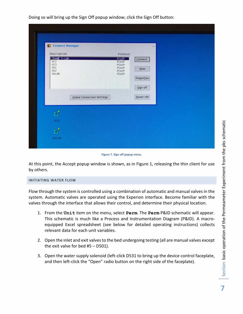
Doing so will bring up the Sign Off popup window; click the Sign Off button:

Figure 7. Sign off popup menu.

At this point, the Accept popup window is shown, as in Figure 1, releasing the thin client for use by others.

INITIATING WATER FLOW

Flow through the system is controlled using a combination of automatic and manual valves in the system. Automatic valves are operated using the Experion interface. Become familiar with the valves through the interface that allows their control, and determine their physical location.

1. From the Unit item on the menu, select Perm. The Perm P&ID schematic will appear. This schematic is much like a Process and Instrumentation Diagram (P&ID). A macro-equipped Excel spreadsheet (see below for detailed operating instructions) collects relevant data for each unit variables.

2. Open the inlet and exit valves to the bed undergoing testing (all are manual valves except the exit valve for bed #5 – D501).

3. Open the water supply solenoid (left-click D531 to bring up the device control faceplate, and then left-click the “Open” radio button on the right side of the faceplate).

Sect

ion

: U

sin

g th

e Ex

cel D

ata

Co

llect

or

8

4. Open the water flow control valve (left-click F531 to bring up the controller faceplate, enter an OP of 20-30% to start water flowing through the bed). Raise flow rate as necessary to reach assigned targets.

5. Monitor differential pressure across the beds (see P502 at the top of the schematic), trying to keep it below the maximum readout of 250 inches water. For some beds this is impossible. Use the Bourdon pressure gauge instead.

6. After a few moments, visually confirm that water is flowing to the drain.

7. Open the bypass valve on the differential pressure gauge to purge air from the pressure lines. Re-close this valve after a minute or two.

8. Switch F531 to AUTO and adjust the setpoint (it is in ml/min) until achieving the desired flow rate.

SHUTTING DOWN SYSTEM

1. Close the water flow control valve (i.e., left-click F531 to bring up the controller faceplate, left-click the SP field to enter a value of 0.0., left-click the MD dropdown list box and select MAN, left-click the OP field and enter a value of -6.9).

2. Close the water supply solenoid valve (left-click D531 to bring up the device control faceplate, left-click the “Closed” radio button on the right side of the faceplate).

3. Close the block valves and any of the unit’s solenoid valves in use.

USING THE EXCEL DATA COLLECTOR

On the Desktop, look for a folder named

Excel SpreadSheets

Within that folder, open the folder named

snr

and double click on PermRecorder.xls. The workbook will open with a Start button, the experiment name, a drop-down menu box for collection frequency, and a Stop button on the

top line.

Click on the Start button, and the workbook will start collecting the relevant data at a collection frequency chosen from the drop-down menu. When ready to save the data, press the Stop button, cut/paste the data into another instance of Excel, and then save this second instance wherever needed. Note that during data collection, conducting any activity in this instance of Excel other than scrolling around to look at the data, may stop the collector and require restarting. Note: The Experion system does NOT collect Ocean Optics data. See instructions for this activity below.

Sect

ion

: P

erfo

rmin

g a

Trac

er T

est

– W

ater

Flo

w

9

PERFORMING A TRACER TEST – WATER FLOW

Ultraviolet (UV) or visible-range (VIS) spectroscopy provides the means to measure the concentration of effluent tracers. An online and offline analyzer probe (Ocean Optics UV dip probe) is the actual sensing element. This probe requires careful handling. Nothing (no solid object, especially) should ever enter the cavity of the probe except the process fluid or distilled water for cleaning. Never place the probe on a dirty surface. The default location for the probe is the mounting mechanism in the effluent flow line. However, an instructor can remove the probe to allow students to make batch readings for calibration or other purposes.

Be sure to turn off the lamps at the end of a lab period, to prolong their life.

The Ocean Optics spectrometer itself resides in a module (connected to the PC through a USB port) near the experiment. Fiber-optic cables transmit the radiation from the DT-1000 source to the dip probe and the detected signal to the PC.

To perform calibration and then conduct a tracer experiment, use the following procedure.

1. Power up the spectrometer equipment.

To do this, first be sure that the Silex Technology USB hub/network connector is powered up and the rocker power switch at the rear of the Ocean Optics spectrometer is in the ON or 1 position. Then, press both the UV Start and Visible Start buttons on the front of the spectrometer. These two buttons turn on the specific light sources.

2. Enable USB communication from the Permeameter spectrometer.

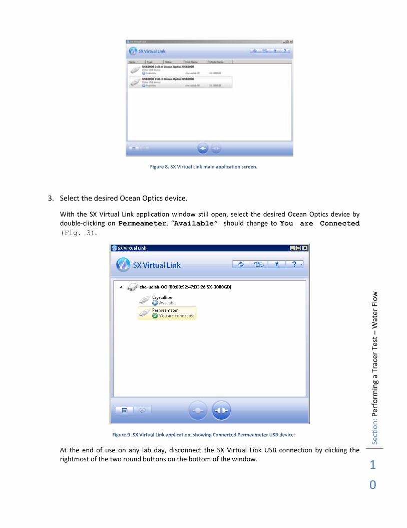
From a separate thin client, log into either the OO1 or OO2 virtual machine (see page 5 to locate these icons) by double-clicking its icon. Locate the SX Virtual Link icon on the virtual desktop and double-click to display the main application window for the SX Server Link application, as shown in Figure 8. This display should show two Ocean Optics USB 2000 devices, one for the Permeameter (given by location 2.41.0) and one for the Crystallizer (given by location 2.41.3). If these do not appear on

this display, disconnect and reconnect the power to the field USB hub. After the hub completes its self-test cycle, these two devices should appear on this display. If not, contact the Lab Coordinator.

Sect

ion

: Per

form

ing

a Tr

acer

Te

st –

Wat

er F

low

1

0

Figure 8. SX Virtual Link main application screen.

3. Select the desired Ocean Optics device.

With the SX Virtual Link application window still open, select the desired Ocean Optics device by double-clicking on Permeameter. “Available” should change to You are Connected

(Fig. 3).

Figure 9. SX Virtual Link application, showing Connected Permeameter USB device.

At the end of use on any lab day, disconnect the SX Virtual Link USB connection by clicking the rightmost of the two round buttons on the bottom of the window.

Sect

ion

: Per

form

ing

a Tr

acer

Te

st –

Wat

er F

low

1

1

Please be sure to perform this disconnect operation as no other computer will be able to connect to the Permeameter spectrometer until the connection is closed!

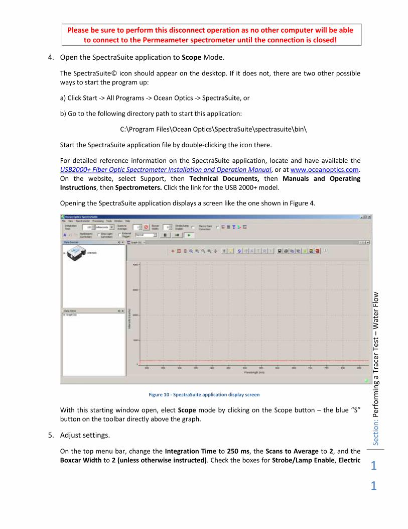
4. Open the SpectraSuite application to Scope Mode.

The SpectraSuite© icon should appear on the desktop. If it does not, there are two other possible ways to start the program up:

a) Click Start -> All Programs -> Ocean Optics -> SpectraSuite, or

b) Go to the following directory path to start this application:

C:\Program Files\Ocean Optics\SpectraSuite\spectrasuite\bin\

Start the SpectraSuite application file by double-clicking the icon there.

For detailed reference information on the SpectraSuite application, locate and have available the USB2000+ Fiber Optic Spectrometer Installation and Operation Manual, or at www.oceanoptics.com. On the website, select Support, then Technical Documents, then Manuals and Operating Instructions, then Spectrometers. Click the link for the USB 2000+ model.

Opening the SpectraSuite application displays a screen like the one shown in Figure 4.

Figure 10 - SpectraSuite application display screen

With this starting window open, elect Scope mode by clicking on the Scope button – the blue “S” button on the toolbar directly above the graph.

5. Adjust settings.

On the top menu bar, change the Integration Time to 250 ms, the Scans to Average to 2, and the Boxcar Width to 2 (unless otherwise instructed). Check the boxes for Strobe/Lamp Enable, Electric

Sect

ion

: Per

form

ing

a Tr

acer

Te

st –

Wat

er F

low

1

2

Dark Correction, and Stray Light Correction. No other boxes should contain checks. Do not change any other parameters on the top menu bar.

6. Prepare Dark Spectrum and Reference Spectrum files.

The spectrometer – to give meaningful results – will require the generation of a Dark Spectrum file and a Reference Spectrum file.

a) Immerse the probe into a test tube filled with DI water. Be sure to completely secure the probe mirror/cap to the probe. A partially secured mirror/cap (i.e., not completely screwed on) will negatively affect your readings.

b) To create a Dark Spectrum file, unplug the probe from the light source (white box). The ensuing graph should nearly trace the x-axis. When the probe has no light source, and the detector has no light reaching it, the spectrum generated is called a Dark Spectrum. To save this newly created Dark Spectrum, click on the grey light bulb (labeled Store Dark Spectrum). An alternative method is to save this spectrum through File -> Store -> Store Dark Spectrum.

c) To create a Reference Spectrum file, plug the probe connection back into the light source. Some peaks should appear on the graph in SpectraSuite. To save this Reference Spectrum, click on the yellow light bulb button (labeled Store Reference Spectrum). An alternative method is to save this spectrum through File -> Store -> Store Reference Spectrum.

d) Both of these saved files – the dark and reference spectra – will serve as reference points throughout the calibration process. It may be possible to use these saved files over and over again, without having to generate them every time the spectrometer is in use – this is the purpose of saving these files in the first place. However, there is nothing wrong with regenerating them each day.

e) If ANY settings change (e.g., Integration Time), both the Dark Spectrum and Reference Spectrum must be generated again.

7. Create a set of suitable calibration standards.

Make these from fluorescing dyes (a visible spectrum tracer) or reagent potassium iodide solution (a near UV tracer). The Instructor will specify. The discussion below assumes fluorescent dyes.

a) Reasonable calibration requires a minimum of four standard samples, though even more standard samples reduce uncertainty and to deal with nonlinearity (if this is evident). A fifth standard is deionized (DI) water.

b) The concentration of the pre-made standards – both red and yellow-green fluorescent dyes – is 250 ppm. Therefore dilution is necessary.

c) One reasonable series of low-level calibration standard concentrations, for either dye, might be 1, 2, 3 and 4 ppmw.

The actual standards concentrations are not critical. However, none of them should result in a spectrometer absorbance reading greater than 1.

Using 250 ppm pre-made standard, make a 25 ppm working standard by adding 450 mL of DI water to 50 mL of the pre-made standard in a 500 mL volumetric flask.

Sect

ion

: Per

form

ing

a Tr

acer

Te

st –

Wat

er F

low

1

3

To prepare the low-level calibration standards, make further dilutions with DI in 25 mL volumetric flasks, employing the following equations to determine the final solution volume and thus the amount of DI water to add:

- - - - - -working standard to add working standard to add desired-low-level-solution desired-low-level-solutionV C V C (1.1)

For example, to create a 25 mL low-level calibration standard at 2 ppm from a 25 ppm yellow-green fluorescent dye working standard, it is evident that:

25 ppm 25 mL 2 ppm

2 mL

working-standard -to-add

working-standard -to-add

V

V

(1.2)

So, to make up this low-level calibration standard – a 2 ppm standard – use 2 mL of the more-concentrated working standard and 23 mL of DI water.

8. Run these low-level calibration standards on the Permeameter spectrometer.

a) Pour these standards into aluminum foil-covered test tubes. One tube should contain only DI water and one each for the low-level standards prepared. Be sure to have each tube labeled appropriately.

b) With the Dark and Reference Files stored on SpectraSuite, click on the Absorbance button (blue “A” located immediately above the graph). Before beginning, a good rule of thumb is to start with the lowest concentration (water itself) and finish with the highest concentration.

c) With the probe in the water test tube, click on the “Strip Chart” button (far right button on the

uppermost menu bar, the icon is a graph with a red and green line on it). The current setting should now be the Single Wavelength setting. For red, use 550nm, while 486nm works best for yellow-green. Use the arrow keys next to the values to select wavelengths; typing in these wavelengths does not work. SpectraSuite™ will not save these but will refer to defaults.

d) After clicking Accept, a new graph will appear, and the program will plot the data. When the line

reaches the end of the screen, click the Save button (i.e., the button with the disc on it, directly above the graph). In the popup window, highlight the settings for the plotline (there should be only one line listed). Create a folder on the desktop to save this data and data for the remaining standard samples. With this location selected, click Save. It is also necessary to click Save in the Save Trend window in addition to the normal Save procedure; else the data will not save.

e) These steps complete the analysis of the first standard calibration point. Repeat steps 3-5 for

the subsequent standard samples.

f) To retrieve the data, open the previously-created desktop folder. Open the specific file with WordPad. Copy and paste the absorbance data into an Excel file. Create a calibration curve of concentration versus average absorbance.

9. Perform tracer tests in the Permeameter using dye standards.

a) Ensure that the manual inlet and outlet valves corresponding to the bed of interest are open.

b) Insert the spectrometer probe into the sample point. Unscrew the cap and then extend the plunger. To achieve a water-tight seal, ensure the use of the metal collar located within the

Sect

ion

: Per

form

ing

a Tr

acer

Te

st –

Wat

er F

low

1

4

sample point cap (including the O-ring) on the probe itself. Carefully guide the probe into the sample point.

c) Open the water supply valve on Station by clicking on D531.

d) Begin to flow water into the unit: Click on F531 (water flow control valve). Enter an OP valve of

20-30% to start water flowing into the unit.

e) Monitor the differential pressure (d/p transmitter) using P502 (top of the schematic, units = inches of water). The span of the d/p is 250 inches of water. For higher differential pressures, use the Bourdon pressure gauge instead.

f) Visually confirm that water is flowing to the drain. Also, confirm that no water is flowing out of

the probe sample point.

g) Purge air from the pressure lines by opening the bypass valve on the d/p transmitter. Close the valve after 1-2 minutes.

h) Change F531 from “MAN” to “AUTO.” Adjust the setpoint until achieving the assigned flowrate

(in mL/min).

i) Verify that the UV/Vis software is loaded and ready to read and the spectrometer is online.

j) When water begins flowing through the unit, the Absorbance profile should match up to the profile of the probe in the test tube of water.

k) Prep for sample injection: Click on D504 and change the status from “Running” to “Charging.”

Doing so will allow loading the sample into the injection valve.

l) Detach the syringe from the unit. Draw approx. 15 mL, attach the loaded syringe back onto the unit and inject the contents into the sample loop. DO NOT detach the syringe after injection while in “Charging” mode, as most of your sample will drain out of the loop.

m) Prepare a Strip Chart to track the passage of the sample across the spectrometer probe. Use the

same protocol for prepping a Strip Chart as done for the Calibration.

n) Once the Strip Chart is ready and a plot displays on the chart (should be a horizontal line at or close to 0), change the status of D504 from “Charging” to “Running.” Introduce the sample into the unit now.

o) After recording data from this sample, save the data using the same protocol for saving data for

calibration points. Make a note of the clock time when this sample begins and ends. When moving the data to Excel, not all of the zero-absorbance points are needed.

p) Clean out the injection chamber: Change the status of D504 from “Running” to “Charging.”

Detach and load the syringe with water, then inject the water into the chamber. Do this at least twice. Change the D504 status to “Running” and let the unit water flow for 5 minutes.

q) Flush the unit lines: The dyes used for this experiment can stain and potentially skew future

results if not flushed out. To ensure that traces or remnants of the dye do not coat the walls of

Sect

ion

: Per

form

ing

a Tr

acer

Te

st –

Wat

er F

low

1

5

the piping, set the flow rate to 2500 mL/min (or as high as possible) and let flow for 10-15 minutes.

r) When done injecting tracers, click on F531 and change the status from “AUTO” to “MAN.” Set

the %OP to a value of -6. Click on D531 and change the status from “Open” to “Closed.”

s) The water flow should stop. Remove the probe from the sample point. Do this carefully. Place it back into the water-filled test tube. Place the collar and O-ring back into the nut, put the plunger back in its starting position, and re-attach the nut.

t) Turn off the light source, each light individually and then the main on/off switch.

u) Log off the Honeywell Station and SpectraSuite. Be sure to disconnect from the USB2000 on SX

Virtual Link before logging off entirely.

Sect

ion

: Sp

ectr

op

ho

tom

eter

Tro

ub

leSh

oo

tin

g Ti

ps

1

6

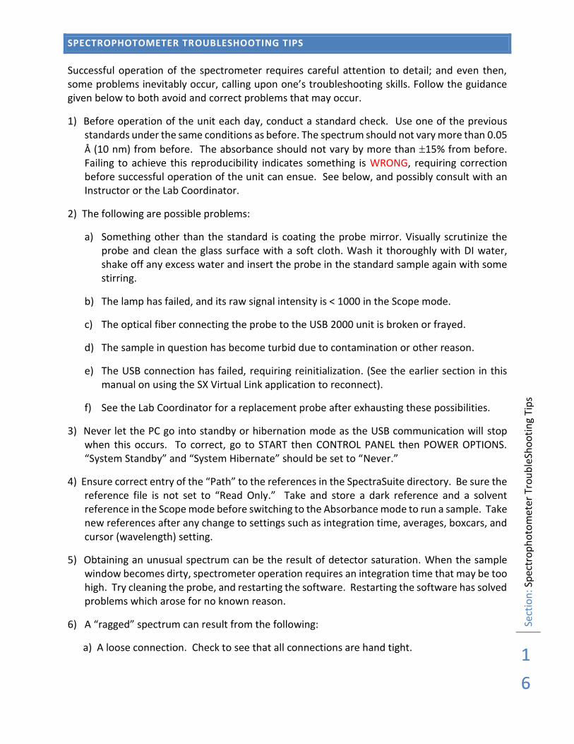
SPECTROPHOTOMETER TROUBLESHOOTING TIPS

Successful operation of the spectrometer requires careful attention to detail; and even then, some problems inevitably occur, calling upon one’s troubleshooting skills. Follow the guidance given below to both avoid and correct problems that may occur.

1) Before operation of the unit each day, conduct a standard check. Use one of the previous standards under the same conditions as before. The spectrum should not vary more than 0.05

Å (10 nm) from before. The absorbance should not vary by more than 15% from before. Failing to achieve this reproducibility indicates something is WRONG, requiring correction before successful operation of the unit can ensue. See below, and possibly consult with an Instructor or the Lab Coordinator.

2) The following are possible problems:

a) Something other than the standard is coating the probe mirror. Visually scrutinize the probe and clean the glass surface with a soft cloth. Wash it thoroughly with DI water, shake off any excess water and insert the probe in the standard sample again with some stirring.

b) The lamp has failed, and its raw signal intensity is < 1000 in the Scope mode.

c) The optical fiber connecting the probe to the USB 2000 unit is broken or frayed.

d) The sample in question has become turbid due to contamination or other reason.

e) The USB connection has failed, requiring reinitialization. (See the earlier section in this manual on using the SX Virtual Link application to reconnect).

f) See the Lab Coordinator for a replacement probe after exhausting these possibilities.

3) Never let the PC go into standby or hibernation mode as the USB communication will stop when this occurs. To correct, go to START then CONTROL PANEL then POWER OPTIONS. “System Standby” and “System Hibernate” should be set to “Never.”

4) Ensure correct entry of the “Path” to the references in the SpectraSuite directory. Be sure the reference file is not set to “Read Only.” Take and store a dark reference and a solvent reference in the Scope mode before switching to the Absorbance mode to run a sample. Take new references after any change to settings such as integration time, averages, boxcars, and cursor (wavelength) setting.

5) Obtaining an unusual spectrum can be the result of detector saturation. When the sample window becomes dirty, spectrometer operation requires an integration time that may be too high. Try cleaning the probe, and restarting the software. Restarting the software has solved problems which arose for no known reason.

6) A “ragged” spectrum can result from the following:

a) A loose connection. Check to see that all connections are hand tight.

Sect

ion

: Rea

ctiv

e (P

arti

tio

nin

g) T

race

rs

1

7

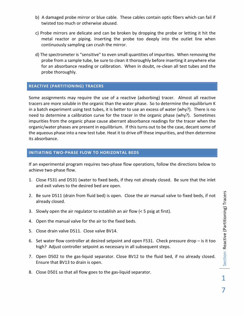
b) A damaged probe mirror or blue cable. These cables contain optic fibers which can fail if twisted too much or otherwise abused.

c) Probe mirrors are delicate and can be broken by dropping the probe or letting it hit the metal reactor or piping. Inserting the probe too deeply into the outlet line when continuously sampling can crush the mirror.

d) The spectrometer is “sensitive” to even small quantities of impurities. When removing the probe from a sample tube, be sure to clean it thoroughly before inserting it anywhere else for an absorbance reading or calibration. When in doubt, re-clean all test tubes and the probe thoroughly.

REACTIVE (PARTITIONING) TRACERS

Some assignments may require the use of a reactive (adsorbing) tracer. Almost all reactive tracers are more soluble in the organic than the water phase. So to determine the equilibrium K in a batch experiment using test tubes, it is better to use an excess of water (why?). There is no need to determine a calibration curve for the tracer in the organic phase (why?). Sometimes impurities from the organic phase cause aberrant absorbance readings for the tracer when the organic/water phases are present in equilibrium. If this turns out to be the case, decant some of the aqueous phase into a new test tube. Heat it to drive off these impurities, and then determine its absorbance.

INITIATING TWO-PHASE FLOW TO HORIZONTAL BEDS

If an experimental program requires two-phase flow operations, follow the directions below to achieve two-phase flow.

1. Close F531 and D531 (water to fixed beds, if they not already closed. Be sure that the inlet and exit valves to the desired bed are open.

2. Be sure D511 (drain from fluid bed) is open. Close the air manual valve to fixed beds, if not already closed.

3. Slowly open the air regulator to establish an air flow (< 5 psig at first).

4. Open the manual valve for the air to the fixed beds.

5. Close drain valve D511. Close valve BV14.

6. Set water flow controller at desired setpoint and open F531. Check pressure drop – is it too high? Adjust controller setpoint as necessary in all subsequent steps.

7. Open D502 to the gas-liquid separator. Close BV12 to the fluid bed, if no already closed. Ensure that BV13 to drain is open.

8. Close D501 so that all flow goes to the gas-liquid separator.

Sect

ion

: Usi

ng

the

Po

lari

met

er –

Su

cro

se In

vers

ion

Rea

ctio

n

1

8

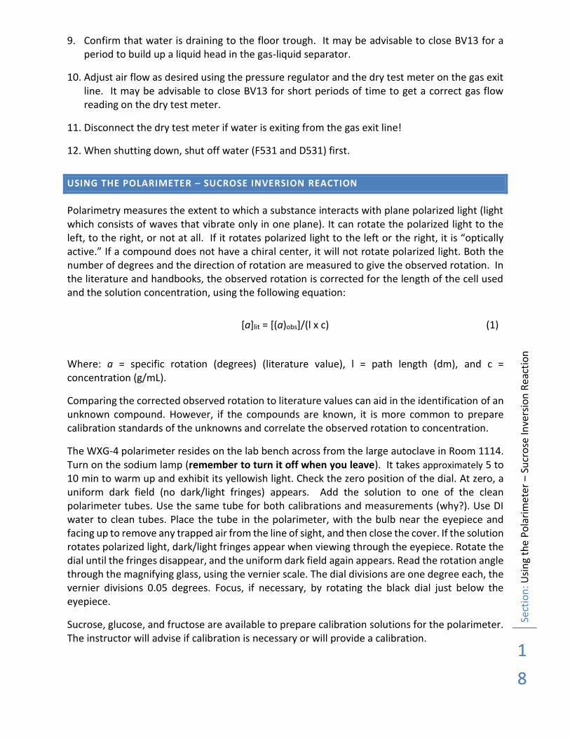
9. Confirm that water is draining to the floor trough. It may be advisable to close BV13 for a period to build up a liquid head in the gas-liquid separator.

10. Adjust air flow as desired using the pressure regulator and the dry test meter on the gas exit line. It may be advisable to close BV13 for short periods of time to get a correct gas flow reading on the dry test meter.

11. Disconnect the dry test meter if water is exiting from the gas exit line!

12. When shutting down, shut off water (F531 and D531) first.

USING THE POLARIMETER – SUCROSE INVERSION REACTION

Polarimetry measures the extent to which a substance interacts with plane polarized light (light which consists of waves that vibrate only in one plane). It can rotate the polarized light to the left, to the right, or not at all. If it rotates polarized light to the left or the right, it is “optically active.” If a compound does not have a chiral center, it will not rotate polarized light. Both the number of degrees and the direction of rotation are measured to give the observed rotation. In the literature and handbooks, the observed rotation is corrected for the length of the cell used and the solution concentration, using the following equation:

[a]lit = [(a)obs]/(l x c) (1)

Where: a = specific rotation (degrees) (literature value), l = path length (dm), and c = concentration (g/mL).

Comparing the corrected observed rotation to literature values can aid in the identification of an unknown compound. However, if the compounds are known, it is more common to prepare calibration standards of the unknowns and correlate the observed rotation to concentration.

The WXG-4 polarimeter resides on the lab bench across from the large autoclave in Room 1114. Turn on the sodium lamp (remember to turn it off when you leave). It takes approximately 5 to 10 min to warm up and exhibit its yellowish light. Check the zero position of the dial. At zero, a uniform dark field (no dark/light fringes) appears. Add the solution to one of the clean polarimeter tubes. Use the same tube for both calibrations and measurements (why?). Use DI water to clean tubes. Place the tube in the polarimeter, with the bulb near the eyepiece and facing up to remove any trapped air from the line of sight, and then close the cover. If the solution rotates polarized light, dark/light fringes appear when viewing through the eyepiece. Rotate the dial until the fringes disappear, and the uniform dark field again appears. Read the rotation angle through the magnifying glass, using the vernier scale. The dial divisions are one degree each, the vernier divisions 0.05 degrees. Focus, if necessary, by rotating the black dial just below the eyepiece.

Sucrose, glucose, and fructose are available to prepare calibration solutions for the polarimeter. The instructor will advise if calibration is necessary or will provide a calibration.

Sect

ion

: Usi

ng

the

Rea

cto

r (B

ed 1

) fo

r Su

cro

se K

inet

ics

Stu

die

s

1

9

USING THE REACTOR (BED 1) FOR SUCROSE KINETICS STUDIES

The sucrose inversion reaction is:

sucrose glucose (dextrose) + fructose (2)

This is an acid-catalyzed reaction and the catalyst (AM-15) is a common industrial solid acid catalyst of the sulfonic acid type – the sulfonic acid groups are attached to a poly (styrene-co-divinylbenzene) backbone. Catalyst properties are: size – 20-40 mesh; weight = 223 g; water content = 30 wt. %; apparent (bulk) density = 1010 kg/m3; acid site concentration = 4.6 mmol acid groups/g dry weight; surface area = 50 m2/g; macroporosity (macropore volume/total volume of cat.) = 0.34; average macropore size = 80 nm.

Activation of the catalyst requires passing 0.25 M sulfuric acid over it. About 2 L of acid should suffice, followed by ~200 mL of DI water. The acid protons will exchange for whatever other ions are attached to the sulfonic acid anions, ‘regenerating’ the catalyst.

The reaction kinetics are usually found to be first order in sucrose concentration and first order in the concentration of catalyst sites. So for a non-deactivating or slowly deactivating catalyst, the reaction kinetics can be approximated by a simple first-order reaction. Of course, like most acid catalysts, some deactivation will take place over time. Lifshutz and Dranoff report a second-order rate constant of ~0.014 g dry cat./(mmol acid sites-min) for a similar catalyst at 60°C, with an activation energy of 77 kJ/mol[2]. Gilliland et al. report ~0.020 g dry cat./(mmol acid sites-min) with an activation energy of 84 kJ/mol, again for a similar catalyst at these conditions [3].

A typical temperature for the reaction is 60°C. Reasonable levels of conversion occur in the range of 80 to 100 mL/min of a 20 wt. % sucrose (in DI water – a MUST) feed. When preparing the sucrose solution, add it slowly to some water, while stirring, at room temperature. Use both a magnetic stirrer and a paddle.

The temperature controller, T505, should be using the following tuning parameters for operation in the 80 to 100 mL/min range near 60°C: Kc = 0.34 %OP/%PV, Ti = 21 min, Td = 5 min. Use T5AVG for the control thermocouple unless instructed otherwise. Implementing control with the specifications just given should allow the unit to move from ambient to 60°C in roughly 45 to 60 minutes and control within 3 to 4°C of the set point, using this average sensor reading (computed from T503 and T502) for temperature control.

When starting the heater up, first place the T505 setpoint (SP) to near (say 10°C below) the process value. Then place the controller in AUTO. When the reactor T first crosses the set point, move the setpoint to the desired final temperature. There may be a temperature profile across the catalyst section, as can be seen by examining thermocouples T502 and T503. Consider this in experimental design and data analysis.

Do not conduct runs at temperatures greater than 60°C without the express authorization of the instructor. Additionally, recognize these issues:

Sect

ion

: Sh

ut

Do

wn

Pro

ced

ure

fo

r K

inet

ics

Stu

die

s

2

0

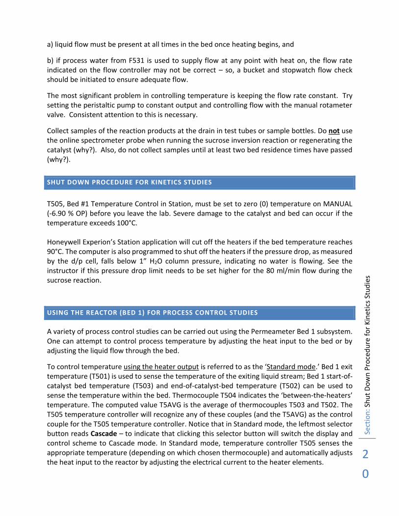
a) liquid flow must be present at all times in the bed once heating begins, and

b) if process water from F531 is used to supply flow at any point with heat on, the flow rate indicated on the flow controller may not be correct – so, a bucket and stopwatch flow check should be initiated to ensure adequate flow.

The most significant problem in controlling temperature is keeping the flow rate constant. Try setting the peristaltic pump to constant output and controlling flow with the manual rotameter valve. Consistent attention to this is necessary.

Collect samples of the reaction products at the drain in test tubes or sample bottles. Do not use the online spectrometer probe when running the sucrose inversion reaction or regenerating the catalyst (why?). Also, do not collect samples until at least two bed residence times have passed (why?).

SHUT DOWN PROCEDURE FOR KINETICS STUDIES

T505, Bed #1 Temperature Control in Station, must be set to zero (0) temperature on MANUAL (-6.90 % OP) before you leave the lab. Severe damage to the catalyst and bed can occur if the temperature exceeds 100°C. Honeywell Experion’s Station application will cut off the heaters if the bed temperature reaches 90°C. The computer is also programmed to shut off the heaters if the pressure drop, as measured by the d/p cell, falls below 1” H2O column pressure, indicating no water is flowing. See the instructor if this pressure drop limit needs to be set higher for the 80 ml/min flow during the sucrose reaction.

USING THE REACTOR (BED 1) FOR PROCESS CONTROL STUDIES

A variety of process control studies can be carried out using the Permeameter Bed 1 subsystem. One can attempt to control process temperature by adjusting the heat input to the bed or by adjusting the liquid flow through the bed.

To control temperature using the heater output is referred to as the ‘Standard mode.’ Bed 1 exit temperature (T501) is used to sense the temperature of the exiting liquid stream; Bed 1 start-of-catalyst bed temperature (T503) and end-of-catalyst-bed temperature (T502) can be used to sense the temperature within the bed. Thermocouple T504 indicates the ‘between-the-heaters’ temperature. The computed value T5AVG is the average of thermocouples T503 and T502. The T505 temperature controller will recognize any of these couples (and the T5AVG) as the control couple for the T505 temperature controller. Notice that in Standard mode, the leftmost selector button reads Cascade – to indicate that clicking this selector button will switch the display and control scheme to Cascade mode. In Standard mode, temperature controller T505 senses the appropriate temperature (depending on which chosen thermocouple) and automatically adjusts the heat input to the reactor by adjusting the electrical current to the heater elements.

Sect

ion

: Usi

ng

the

Rea

cto

r (B

ed 1

) fo

r P

roce

ss C

on

tro

l Stu

die

s

2

1

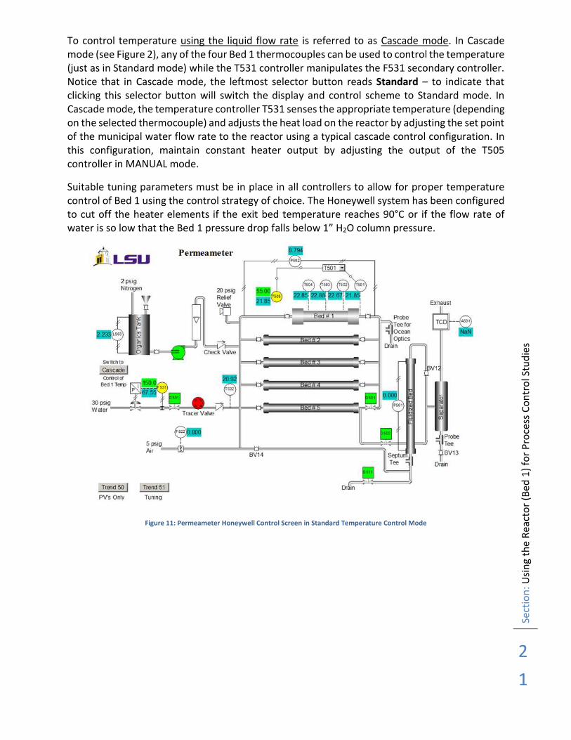
To control temperature using the liquid flow rate is referred to as Cascade mode. In Cascade mode (see Figure 2), any of the four Bed 1 thermocouples can be used to control the temperature (just as in Standard mode) while the T531 controller manipulates the F531 secondary controller. Notice that in Cascade mode, the leftmost selector button reads Standard – to indicate that clicking this selector button will switch the display and control scheme to Standard mode. In Cascade mode, the temperature controller T531 senses the appropriate temperature (depending on the selected thermocouple) and adjusts the heat load on the reactor by adjusting the set point of the municipal water flow rate to the reactor using a typical cascade control configuration. In this configuration, maintain constant heater output by adjusting the output of the T505 controller in MANUAL mode.

Suitable tuning parameters must be in place in all controllers to allow for proper temperature control of Bed 1 using the control strategy of choice. The Honeywell system has been configured to cut off the heater elements if the exit bed temperature reaches 90°C or if the flow rate of water is so low that the Bed 1 pressure drop falls below 1” H2O column pressure.

Figure 11: Permeameter Honeywell Control Screen in Standard Temperature Control Mode

Sect

ion

: Sh

ut

Do

wn

Pro

ced

ure

fo

r C

on

tro

l Stu

die

s

2

2

Figure 12: Permeameter Honeywell Control Screen in Cascade Temperature Control Mode

SHUT DOWN PROCEDURE FOR CONTROL STUDIES

Use the following steps to ensure leaving the Permeameter in a suitably safe mode after conducting Bed 1 control studies:

Place the unit display into the Standard mode.

Change the setpoint of T505 to 0°C.

Place controller T505 in MANUAL mode and set its output to -6.9%.

If the heater has been on and the bed temperature is elevated, raise the water flow rate (F531) to 2000 cc/min and wait till the temperature of the exiting stream is less than 30C.

Place controller F531 in MANUAL mode and set its output to -6.9%.

Severe damage to the catalyst and bed can occur if the temperature exceeds 100°C.

INITIATING AIR FLOW TO VERTICAL (FLUIDIZED) BED AND GAS TRACER INJECTION

Use the same Steps 1 through 3 described earlier for introducing two-phase flow.

4. Close D511 (drain from fluid bed) and BV13 from the separator to the drain.

5. Confirm that air is exiting from the line near the gas cylinders.

6. Monitor differential pressure across the bed (see the “Fluid Bed del(P)” graphic).

Sect

ion

: In

itia

tin

g A

ir F

low

to

Ver

tica

l (Fl

uid

ized

) B

ed a

nd

Gas

Tra

cer

Inje

ctio

n

2

3

7. Open the rotameters to the “Sample” and “Reference” sides of the TCD detector to near their maximum values (2.0). They should be kept equal.

8. Turn on power to TCD detector; using the “Zero” knob, zero the signal. Check for zero on the computer also. It does not have to be precisely zero, just near zero and stable.

9. The inert tracer for the gas phase experiments is CO2. The tracer must be syringe-injected using a LARGE syringe with a 25 G needle. Turn the CO2 cylinder on and adjust regulator pressure until reaching ~5 psig at the sample point. Keeping some pressure on a syringe, insert it into the sample point, and allow it to fill. Then, after noting the time, inject the sample at the injection point below the fluidized bed.

10. Note the need to periodically check for leaks at the sample and injection points and replace septa as necessary. Use Snoop to check for leaks.

Sect

ion

: Ref

eren

ces

2

4

REFERENCES

[1] W. L. McCabe, J. C. Smith, and P. Harriott, Unit operations of chemical engineering, 7th ed. Boston: McGraw-Hill, 2005.

[2] N. Lifshutz and J. S. Dranoff, "Inversion of Concentrated Sucrose Solutions in Fixed Beds of Ion Exchange Resin," Industrial & Engineering Chemistry Process Design and Development, vol. 7, pp. 266-269, 1968.

[3] E. R. Gilliland, H. J. Bixler, and J. E. O'Connell, "Catalysis of Sucrose Inversion in Ion-Exchange Resins," Industrial & Engineering Chemistry Fundamentals, vol. 10, pp. 185-191, 1971.