Embed Size (px)
DESCRIPTION
MILTON FRIEDMAN AND THE EMERGENCE OF THE PERMANENT INCOME HYPOTHESIS
Citation preview
1
MILTON FRIEDMAN AND THE EMERGENCE OF THE
PERMANENT INCOME HYPOTHESIS
Hsiang-Ke Chao∗∗∗∗
University of Amsterdam
November 2000
ABSTRACT
The purpose of this paper is to investigate the evolution of Milton Friedman’s permanent income
hypothesis from the 1940s to 1960s, and how it became the paradigm of modern consumption
theory. Modelling unobservables, such as permanent income and permanent consumption, is a
long-standing issue in economics and econometrics. While the conventional approach has been to
set an empirical model to make “permanent income” measurable, the historical change in the
meaning of that theoretical construct is also of methodological interest. This paper will show that
the concepts of unobservables, especially permanent income, in Friedman’s work was fluid and
depended on the instruments used.
This paper was prepared for the European Conferences on the History of Economics at Erasmus Institute for
Philosophy and Economics, Erasmus University Rotterdam, the Netherlands, on 20-22 April 2000. I would like to
thank Mark Blaug, Marcel Boumans, Jim Thomas, Kevin Hoover, members of the LSE-Amsterdam measurement
group and the participants of ECHE 2000 for their comments. I particularly thank Mary Morgan for her comments
and encouragement. All errors are mine.
2
1. INTRODUCTION
In the early stage of his professional career, Milton Friedman worked on consumption theory,
exploring the possible explanations of the relationship between consumption and income, for two
decades. The well-known “permanent income hypothesis”, often connected with his seminal
book A Theory of the Consumption Function (1957), highlights Friedman’s achievement in this
field. Nonetheless, the permanent income hypothesis also raises the issue of defining and
measuring “permanent income”, which unavoidably correlates with performing the same tasks
on “income”. The modern definition of income is owed to Hicks’s book Value and Capital
(1939; 1946 2nd edn.) that identified income as the budget constraint of consumption behavior.
But Hicks needed more specific definitions for empirical purposes. He claimed in his book that
there are still great discrepancies between the theoretical definition and the empirical one and
that existing theories couldn’t help us with these discrepancies, i.e. the measurement problem.
Thus he concluded that these income theories are “bad tools, which break in our hands” (1946,
p.177).
While Hicks attempted to find a satisfactory empirical counterpart for a theoretically sound
definition of income, other economists were conducting empirical studies of income structure.
Among them, Kuznets was the most notable one. Apart from a series of works in the 1930s and
1940s on the measurement of national income, Kuznets started a study comparing incomes of
different professions in 1933 by using data for 1929-32. He completed a draft in 1936 but
Friedman took up the work in 1937 and provided a more detailed statistical analysis1. The result
1 See Friedman and Kuznets (1945), pp. xi-xii.
3
was published in 1945 entitled Income from Independent Professional Practice, by which
Friedman earned his doctoral degree at Columbia University in 1946.
Income from Independent Professional Practice gives an account of income structure:
income is composed of permanent, quasi-permanent and transitory components. It also marks the
first of three stages of Friedman’s research on the permanent income hypothesis. Each stage
corresponds to a different concept of permanent income. In the second stage, identified by A
Theory of Consumption Function, Friedman continued to work on the dichotomy of measured
income but extended it to the account of consumer behavior, i.e., the permanent income
hypothesis. A formal statement of the permanent income hypothesis was given, several empirical
models were built and tests for various types of data were proposed. Consequently this book is
regarded as ‘one of the masterpieces of modern econometrics’ (Blaug, 1998, p.69). Finally,
Friedman (1963) extended the treatment in Friedman (1957, Chapter V) that adopted Cagan’s
adaptive expectations hypothesis (Cagan, 1956) to the case of time-series data. By doing so the
permanent income is equivalent to the adaptive expected income. It became the most popular
version of permanent income.
Several surveys have explored the permanent income hypothesis extensively, namely, Mayer
(1972), Hirsch and De Marchi (1990) and Hynes (1998). Mayer’s book is the most well-known
among them. Mayer indicates three definitions of permanent income in Friedman’s work:
M1 Permanent income is whatever the household thinks it is.
M2 Permanent income is equal to the household’s wealth times the relevant discount rate
M3 Permanent income is an exponentially weighted average of past incomes plus a trend.
4
Nonetheless, the main task of Mayer’s book is to scrutinize the existing tests with respect to
various data in order to appraise the permanent income hypothesis. But the interplay between
data, models and theoretical definitions that appears in the permanent income hypothesis
received less attention.
Both Hirsch and De Marchi (1990) and Hynes (1998) see Friedman’s permanent income
hypothesis as attempting to give a more empirically adequate account of consumption behavior,
in the sense that the permanent income model is made “operational” by containing certain
auxiliary statistical restrictions such that the permanent income hypothesis is capable of being
subject to diagnostic testing. Hynes makes a stronger claim: namely that this modelling process
goes in tandem with operationalism, which implies that the modelling procedure dictates the
definition of the theoretical construct. Yet, such a claim does not completely fit Friedman’s
widely known methodological instrumentalist position. Such claims of operationalism need to be
further justified.
This paper will illustrate the changing concept of the permanent income and the
corresponding stages in Friedman’s work on the permanent income hypothesis from the 1940s to
60s. Moreover, it also deals with the relations between the theoretical concepts, modelling
procedures and different empirical evaluation methods and problems there encountered. Two
empirical problems will be addressed: measurement and testing. Hicks regards models that
improve the measurability of economic entities as good tools, but Friedman is more concerned
with testing models. The conventional view on testing in economics is that tests always confirm
or disconfirm the target theory or model. Friedman’s case on the permanent income hypothesis
can be said to present an alternative idea of testing, namely the “characteristics tests”, meaning
that only certain features of models are subject to test (Kim et al, 1995). Whether models are
5
instruments for measuring or testing the permanent income hypothesis, they interact with the
meaning of permanent income in different ways.
2. MODELLING INCOME STRUCTURE
The aim of the analysis presented in Income from Independent Professional Practice was to
explain income differences among professions. The authors argued that given the free market
mechanism, people with similar ability would receive the same return. The observation of
income differences might suggest also the importance of the difference in institutional factors
such as professional training, the attractiveness and risks of the profession and the like (Friedman
and Kuznets, 1945, pp. v-vii). They conjectured that income differences are a compensation for
longer training -- to equalize differences-- in a free market economy2. Thus, apart from the
description of the income structure, the classification of income determinants is also needed to
interpret income differences. Since Friedman and Kuznets thought that income differences are
determined by human capacities and institutional factors which affect income in different time
spans, the taxonomy of income provides means to categorize the determinants of income by the
length of period that a factor influences income. The components are called permanent if they are
common over the specific time period, that is, “personal attributes such as training, ability,
personality”, or attributes of men’s practice, such as “location, type, organization” and the like
(Friedman and Kuznets, 1945, p.325). That is, permanent components are those effects on
2 The authors concluded that the income differences between occupations are not the equalizing type for there are
obstacles, such as high training fee, to present people from freely choose their occupations. On the other hand,
movement within a profession is unhindered so that the income inequalities of a profession equalize the difference
reflecting differences in age, location and the like. (See Friedman and Kuznets, 1945, ch.3).
6
income which are present in the whole period of investigation. Transitory components, on the
other hand, are defined as the factors whose effects on income exist within the single time unit.
The remaining factors are grouped under the category ‘quasi-permanent components’. The
authors wrote that:
The dichotomy between permanent and transitory components of a man’s income... necessarily
does violence to the facts. An accurate description of the factors determining a man’s income
must substitute a continuum for the dichotomy. This continuum is bounded at one extreme by
“truly” permanent factors- those that affect a man’s income throughout his career-and at the other
by the “truly” transitory- those that affect his income only during a single time unit, where the
time period is the shortest period during which it seems desirable to measure income. ... Between
these extremes falls what may be called “quasi-permanent” factors, factors whose effects neither
disappear at once nor last through out a man’s career (Friedman and Kuznets, 1945, p.352).
In other words, these three components are distinguished by the period they cover. For
example, if a survey of income covers a three-year span, then the permanent components are
those whose affect on income lasts for three or more years; the transitory components are those
whose affects on income occur within the time unit, e.g. one year. Quasi-permanent components
then might be two-year component, or a three-year component finished on the second year, and
so forth.
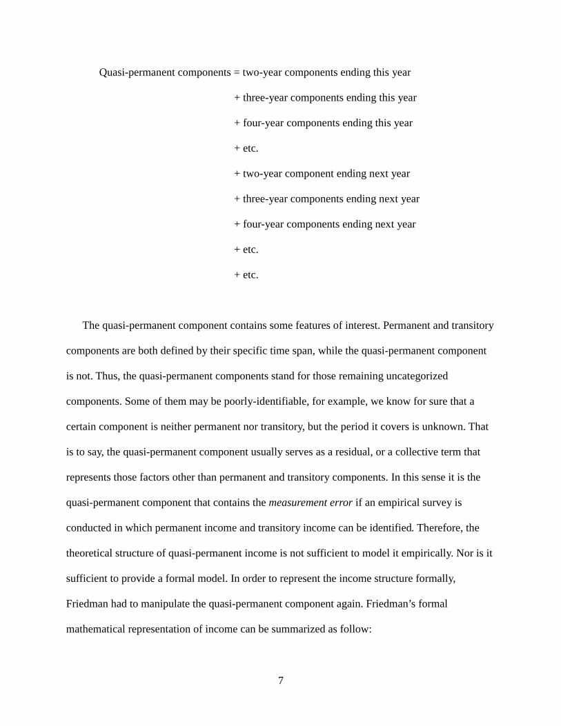
In distinction to the other permanent income accounts, quasi-permanent components take part
without been adequately identified. Friedman suggested a description of the quasi-permanent
components that can be stated as follow (Friedman and Kuznets, 1945, p.353):
7
Quasi-permanent components = two-year components ending this year
+ three-year components ending this year
+ four-year components ending this year
+ etc.
+ two-year component ending next year
+ three-year components ending next year
+ four-year components ending next year
+ etc.
+ etc.
The quasi-permanent component contains some features of interest. Permanent and transitory
components are both defined by their specific time span, while the quasi-permanent component
is not. Thus, the quasi-permanent components stand for those remaining uncategorized
components. Some of them may be poorly-identifiable, for example, we know for sure that a
certain component is neither permanent nor transitory, but the period it covers is unknown. That
is to say, the quasi-permanent component usually serves as a residual, or a collective term that
represents those factors other than permanent and transitory components. In this sense it is the
quasi-permanent component that contains the measurement error if an empirical survey is
conducted in which permanent income and transitory income can be identified. Therefore, the
theoretical structure of quasi-permanent income is not sufficient to model it empirically. Nor is it
sufficient to provide a formal model. In order to represent the income structure formally,
Friedman had to manipulate the quasi-permanent component again. Friedman’s formal
mathematical representation of income can be summarized as follow:
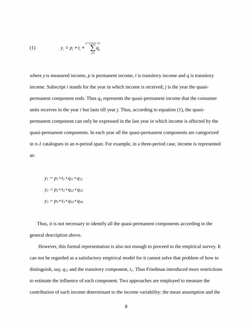
8
(1) �−+−
=
++=)1()1( ni
ijijiii qtpy
where y is measured income, p is permanent income, t is transitory income and q is transitory
income. Subscript i stands for the year in which income is received; j is the year the quasi-
permanent component ends. Thus qij represents the quasi-permanent income that the consumer
units receives in the year i but lasts till year j. Thus, according to equation (1), the quasi-
permanent component can only be expressed in the last year in which income is affected by the
quasi-permanent components. In each year all the quasi-permanent components are categorized
in n-1 catalogues in an n-period span. For example, in a three-period case, income is represented
as:
y1 = p1+t1+q11+q12
y2 = p2+t2+q22+q23
y3 = p3+t3+q33+q34
Thus, it is not necessary to identify all the quasi-permanent components according to the
general description above.
However, this formal representation is also not enough to proceed to the empirical survey. It
can not be regarded as a satisfactory empirical model for it cannot solve that problem of how to
distinguish, say, q11 and the transitory component, t1. Thus Friedman introduced more restrictions
to estimate the influence of each component. Two approaches are employed to measure the
contribution of each income determinant to the income variability: the mean assumption and the
9
variability assumption. The mean assumption is that permanent and quasi-permanent
components change in proportion to the change in the arithmetic mean income of the group,
given that components are uncorrelated with one another-- which is called the zero correlation
assumption. As the standard deviations of components can be derived, we can calculate the
proportionate contribution of each of the three types of components to the total variance of
income in any year. But the mean assumption approach is not sustainable. The problem lies in
the inseparability of quasi-permanent income and transitory income for the reason mention
above.
The variability assumption states that both the standard deviation of permanent and quasi-
permanent components are proportional to the standard deviation of measured income (but not to
the standard deviation of transitory income). It also requires the assumption of zero correlation,
but it has to be further assumed that the proportional contribution of the permanent component is
the same in all years. Although under the variability assumption we can calculate the
contribution of each component, Friedman did not think this assumption reasonable, for if
permanent component and transitory component are uncorrelated and average permanent income
is equal to average measured income, then it implies that the standard deviation of the permanent
component is proportional to the standard deviation of the transitory component. Friedman
argued that this is not reasonable for, by “theory”, the transitory component should contribute a
greater proportion to the variability of measured income than the permanent and quasi-permanent
components. Therefore, the mean assumption is preferable.
The problem confronting Friedman is the measurement of vaguely defined theoretical
constructs that do not translate the implicit causal account into a direct measurable structure. It is
possible to measure the income components only indirectly by looking at the proportional
10
contributions of income variance. Friedman’s measurement of income in Income of Independent
Professional Practice and the other early consumption studies are of methodological interest to
economists. Hirsch and De Marchi (1990) and Hynes (1998) both address the importance of the
operational meaning in the income structure model. Friedman’s work is regarded as being in the
tradition of the “operational development of income structure” (e.g., Hynes, 1998). But a theory
that is operational does not necessarily imply operationalism, which is what Hynes suggests. To
Hynes the term “operational” simply means a theory is model-able to the empirical level; that is,
we can model a theory such that it fits the data (Hynes, 1998, pp.33-4). Defining an
operationalist approach, however, requires that a theoretical term is defined by a set of
operations, i.e. procedure of measurement. If we want to claim Friedman’s approach at this stage
consisted of operationalism, the only way to argue is that these income components depend on
the measurement processes because a component is determined to be permanent or transitory by
the length of time period in which it affects income. For instance, the transitory component is
defined as a component that only affects income in the unit of time, which is decided mainly
under the consideration of data availability. It also means that the transitory components may be
defined by different units of time, so different concepts of transitory income are involved.
Claiming that the income structure is operational by employing the mean and variability
assumptions does not mean we can directly measure these income components. At least no direct
measurement of permanent and transitory income was conducted at this stage. In Income from
Independent Professional Practice, the income of different professions is measured by
questionnaires to professional men sent out by U.S. Department of Commerce (p.47). According
to the questionnaires (Appendix C) income is defined as labor income (i.e., receipts from
11
practice), implying that the concept of Hicksian income doesn’t come into Friedman’s first
formation of permanent income.
3. PERMANENT INCOME HYPOTHESIS-- BUDGET STIDIES
Before Friedman addressed the permanent income hypothesis in A Theory of the Consumption
Function (Friedman, 1957), several consumption theories were proposed to explain the stylized
facts for which Keynes’s absolute income hypothesis failed to give an account. This well-known
Kuhnian history3 starts with the discoveries of theoretical tools and empirical facts. On the
theoretical aspect, Friedman rediscovered the Fisherian intertemporal decision theory (Fisher,
1907) and emphasized his contention that the consumer smoothes his or her expenditures by
borrowing and lending. Friedman claimed that the Fisherian approach to individual consumption
behavior is the ‘pure theory of consumption behavior’ and that it makes the wealth approach a
more sound account than Keynes’s (Freidman, 1957, p.6). On the empirical aspect, Kuznets
published a study of consumption and saving behavior in 1946 --one year after the publication of
Income from Independent Professional Practice-- that indicated several empirical facts
contradicting the predictions of the absolute income hypothesis. Keynesians argued that
according to the absolute income hypothesis, the marginal propensity to consume (MPC) is less
than the average propensity to consume (APC) and that MPC is less than one; thus (1) the
average propensity to save (APS) increases as income rises; (2) APC decreases as income rise.
(3) When government spending fell from the reached level during World War II, the economy
would move toward recession, and then consumption would decrease. But Kuznets used time-
3 Mayer (1972), Ch. 1, especially pp. 7-8; Hynes (1998).
12
series data dating back to the Civil War to point out that (1) MPC is less than APC in budget data
and short-run time-series data but is equal to APC in the long run; (2) APS and APC did not rise
secularly and (3) private demand increased sharply and APS was sharply lower than in the
interwar period level.
However, Friedman also defined permanent income in the sense of Hicksian income (Hicks,
1936/1945, Ch. XIV). Wealth is depreciated expected receipts (Friedman, 1957, pp.8-9);
therefore income is defined as the amount that a consumer unit can consume while wealth
remains unchanged (p.10). In Chapter II of A Theory of the Consumption Theory (p.17),
permanent income is expressed as:
(2) yp=iW
where i stands for interest rate, W stands for wealth at a certain point of time. Wealth is
depreciated income receipts; income --permanent income-- is defined as the amount that the
consumer unit can consume but leave the wealth unchanged (Friedman, 1957, p.10). In Friedman
(1963), i is regarded as “an undefined term having the dimensions of an interest rate”. Hicksian
income is consistent with the Fisherian intertemporal decision theory in the sense that income is
the present value of a stream of future receipts given the consumer unit’s welfare position
unchanged. It also refers to Mayer’s definition two of the permanent income.
3.1 The Formal Model
In ‘The Methodology of Positive Economics’ (Friedman, 1953) Friedman claims that a
theory contains two parts: a language and a body of substantive hypothesis. A language part
13
functions as an ‘analytical filing system’ that categorizes components (Friedman, 1953, p.7). As
an analytical filing system theory should meet both logical and empirical requirements. Friedman
claims that on the logical aspect, the analytical filing system should (1) be clearly and precisely
defined; (2) be exhaustive; (3) avoid cross-reference, and (4) be convenient to browse. On the
empirical aspect, the filing system should provide an account to organize empirical material, thus
we should be able to find for each category a ‘meaningful empirical counterpart’. Formal logic
shows whether the language part is ‘right’ or ‘wrong’ while the capacity of finding empirical
counterparts shows whether the language is ‘useful’ or not (p.7).
Viewed as a model-building process, Friedman’s account leads towards to an empirical
model. The language part in his methodology is not only a verbal statement but also its formal
representation, such as equation (1), that translates the theoretical claim of the income structure
into a mathematical equation. Note that the language part is merely trivially true if it satisfies
logically consistence; any consistent set of taxonomic criteria will do as well.
Nonetheless, the categorization cannot be claimed to be successful and useful if it fails to
find empirical counterparts. If we may put it this way, Friedman’s methodology of positive
economics is concerned with translating verbal terms to theoretical terms and then to empirical
terms.
The formal permanent income hypothesis can be stated as follows:
(3) ( ) pp yuwikc ,,=
(4) tp yyy +=
(5) tp ccc +=
(6) 0),(),(),( === ttptpt cycorrcccorryycorr
14
where y stands for measured income; c stands for measured consumption; yp is permanent
income; yt is transitory income; cp is permanent consumption; ct is transitory consumption; i is
the interest rate; w is the ratio of nonhuman wealth to permanent income and u stands for factors
such as age, family size etcetera that affect consumer’s preferences4. Equations (3) to (5)
represent the theoretical model of the permanent income hypothesis, stating the hypothetical
relationships between measured constructs and theoretical constructs. Measured income is the
sum of permanent income and transitory income. Similarly, measured consumption is the sum of
its permanent and transitory components. Moreover, the model states the relationship between
theoretical constructs: permanent consumption is a function of permanent income. Equation (3)
asserts the proportional relation between permanent income and permanent consumption, which
is regarded as the critical hypothesis of empirical content.
Zero-correlation assumptions (equation (6)) serve as an important part to make the whole
model operational (e.g. Hirsch and De Marchi, 1990). It assumes that the correlation coefficients
of these variables are zero. The first two correlations (corr(yt, yp) = corr(ct, cp) = 0) represent the
nonstochasticity of the permanent component of income and the permanent component of
consumption respectively. The nonstochasticity is based on the definition of transitory
components and thus they ‘have little substantive content’; then it can be explained as
‘translating the definitions of theoretical constructs into formal representation’ (Friedman, 1957,
pp.26-7). The third correlation, corr(yt, ct) =0, introduces important substantive content into the
permanent income hypothesis. Bodkin (1960), for example, took this assumption as a ‘crucial
postulate’ (p.176) because empirical findings do not always support this assumption. This
4 Or as Holms (1970, p.1159) puts it, u is “any objective factors affecting anticipations”.
15
assumption indicates that transitory income does not affect the consumer unit’s planned
consumption. However, Friedman argued that in fact consumers are able to use their windfall
receipts on planned consumption, whereas windfall receipts are usually statistically recorded as
transitory income. Friedman claimed that unexpected windfall receipts are regarded as transitory
income while expected receipts are regarded as permanent income. It leads to the measurement
problem that empirical notions employed in collecting statistical data are not consistent with the
theoretical meanings posited by the theory and the model. Moreover, it calls the measurement of
consumption into question, i.e., whether consumption should be defined in the ‘use’ sense or in
the ‘purchase’ sense5. On this picture, there is much to say about the empirical content and the
zero correlation between yt and ct as it shows the route of influence from theory to the procedure
of measurement.
3.2 Tests and the Characteristics Test
While the conventional view on testing in economics is about rejecting candidate hypotheses,
Kim et al (1995) assert other types of testing exists in economics and econometrics. There are
confirmationalist tests that (1) secure a basis for belief or look for satisfactoriness of empirical
models and (2) confirm the characteristics of empirical models6. With respect to secure belief, as
Kim et al point out, economists would test to “seek in quantification a secure basis for
consensual belief”, such as using “econometrics as a measuring device to reassure the theorist in
his or her belief (Kim et al, 1995, p.83)”. It seems that tests in A Theory of the Consumption
5 See Friedman (1957) and Mayer (1972), pp.12-16.
6 In their article, four types of test are mentioned: (1) testing to discover error, (2) testing to secure a basis for belief
(3) testing as quality control and (4) tests as confirmations of empirical model characteristics.
16
Function behave as the former that are proposed to secure the belief that consumption is
determined by permanent income. Friedman said that the consistency of the permanent income
hypothesis with data supports the belief that the permanent income hypothesis is a useful tool to
explain “the major apparent anomalies that arise if the observed regression between measured
consumption and measured income is interpreted … as a stable relation between permanent
components” (Friedman, 1957, p.225).
Most economists are concerned with testing the permanent income hypothesis. Mayer’s book
documents the activities of testing the permanent income hypothesis from the 1950s to the 70s.
Nonetheless, none of the tests confirm or disconfirm the entire permanent income hypothesis7.
Even Friedman’s tests are not able to do so:
Friedman presented a wide variety of tests, the results of which are consistent with his theory. But
most of the tests are no more than this; they do not require a full permanent income theory to
explain the observations. They are tests of the direction only, rather than rigorous tests of the full
theory. By “tests of direction” I mean tests which show that two coefficients differ in the direction
predicted by the permanent income theory, but not necessarily by the amount predicted by the
theory (Mayer, 1972, pp.59-60).
The characteristics test refers to a type of tests that target on a specific property of the
empirical model, the model that is derived from theory and is capable of processing quantitative
information. In other words, a characteristics test is to match data characteristics with
characteristics of the empirical model. But when we narrow the theory into the empirical model
serving as a testable hypothesis, it does not guarantee the theory is justified. Kim et al point out
7 See Mayer (1972), p.59.
17
that (1) inference from data characteristics to empirical model characteristics are not unique.
Different empirical models may result in same data characteristics. (2) Inference from empirical
models to theory is not possible for different theories can result in the same empirical models. As
Gilbert (1986) criticized the conventional econometrics approach (average economic regression
(AER) view), an OLS regression can be explained by different theories. Moreover, it is arguable
whether the empirical model captures essential characteristics of the theory. In most of the cases
when we try to produce an empirical model, we try to reduce the theory to a simple testable
characteristic. By doing so the empirical model hardly represents the essences of theory.
Several implications derived from the model were thought to be the key properties of the
permanent income hypothesis: (1) the proportional hypothesis, (2) difference in income
elasticities between permanent and transitory components, (3) zero income elasticity of
consumption for transitory income, (4) the lag hypothesis8. Mayer (1972, p.90) shows that none
of the 16 tests that Friedman proposed in (1957) cover these four major predictions (i.e.
characteristics) of the permanent income hypothesis. These tests are characteristics tests: they
only confirm certain characteristics of empirical model9. These tests support the argument Kim et
al made that the characteristics tests even fail to justify the essential characteristics of the theory.
Mayer argued that “none of the tests support the full permanent income theory in the sense of
8 See Mayer (1972) for detail.
9 Friedman claims that “the two most striking pieces of evidence for the hypothesis are, first, its success in
predicting in quantitative detail the effect of classifying consumer units by the change in their measured income
from one year to another; and, second, its consistency with a body of data that have not heretofore been regarded as
relevant to consumption behavior, namely, data on measured income of individual consumer units in successive
years”. However, it does not say that the evidences support the full model of the permanent income hypothesis.
Horses cannot prove the existence of unicorns.
18
showing that the income elasticity of consumption is zero for transitory income and unity for
permanent income” (1972, p.89)10.
3.3 Windfall Experiment
Having viewed corr(yt, ct) =0 as a crucial assumption, Friedman suggested using National
Service Life Insurance (NSLI) dividends that were paid out to US veterans in January 16, 1950
as windfall income to test it. The NSLI case seemed to be a “controlled experiment” of
consumption behavior (Friedman, 1957, p.215) such that it was somehow regarded as a sort of
crucial test of the permanent income hypothesis. Bodkin (1960) took over Friedman’s suggestion
and found that the MPC for NSLI dividends is 0.72, even greater than the MPC for regular
income (0.56). Although he had reservations about this result, Bodkin concluded that people do
spend transitory income, thus the permanent income hypothesis was not sustainable. But
Friedman (1960) responded that NSLI dividends was not a good measure of transitory income
either, but rather would be a proxy of permanent income because recipients were told that
additional payments would be forthcoming.
The debate raised the issue of the measurement problem, that is, how to find empirical
counterparts according to the definitions chosen. Friedman argued that NSLI is not a good
estimate of windfall income because part of it was expected. Interestingly, Bodkin thought NSLI
dividend was a better proxy of the windfall than others used in the previous test on windfall
payments proposed by Klein and Liviatan (1957). Klein and Liviatan’s windfall proxy was not
legitimate for some components of windfall income are not transitory. For instance, Bodkin
10 It is argued that the proportional hypothesis is another essential characteristic of the permanent income hypothesis
(Mayer), but according to Mayer’s survey, only 4 out of 16 tests check the proportional hypothesis.
19
argued controversially that gambling wins for the professional gamblers are ‘permanent income’
(p.179).
The problem is twofold. Firstly, windfall income is often conflated with transitory income as
windfall income is said to be a transitory element. Contrary to this popular belief, windfall
income is not equivalent to the transitory income11. The relations between windfalls and
permanent income and transitory income is based on equation (2) (i.e., yp=iw). Windfall income
raises wealth at the first place, such that it raises permanent income as well. The windfall income
does not affect the transitory income directly because the transitory income is defined as the
difference between measured income and permanent income. Friedman (1957) saw incomes as
stocks, such that if the discount rate is one-third, one-third of the windfall is permanent income
and two-thirds is transitory income. Friedman (1963) saw incomes as flows; the influence of
windfall on the transitory income depends on (1) the point of time it is received and (2) the
length of accounting period. Consequently, the windfall income is equal to the transitory income
only in some special cases12.
Secondly, the problem results from the vagueness of the definitions. Friedman later claimed
that “the notion of ‘windfall’ is therefore logically identical with that of positive ‘profit’ in the
uncertainty theory of profit” (1963, p.6, fn.3), meaning that windfall is unexpected income
receipts. Hence gambling wins are windfall income but not transitory income. Bodkin’s criticism
11 Bodkin seemed to take windfall income and transitory income as synonyms, so did Mayer (1972). For example,
Mayer (p.93) wrote that “[NSLI] was unexpected, and hence qualifies as a windfall, or transitory income”. He took
the consumption increased by windfall as the consumption out of permanent income, not the consumption of
transitory income per se (1971, pp.39-40). But this account requires independent estimates of consumption from
permanent income and from transitory income. Unfortunately, such estimates do not exist (Mayer, 1971, pp.40-41).
12 See Friedman (1963) pp.15-16 for examples.
20
of Klein and Liviatan might be misleading. Moreover, Friedman admitted that permanent and
transitory incomes are arbitrary concepts: “The division [of permanent and transitory income] is,
of course, in part arbitrary, and just where to draw the line may well depend on the particular
application. Similarly, the dichotomy between permanent and transitory components is a highly
special case (Friedman, 1957, p.22, fn.3). Similarly, Friedman defined the transitory income as a
residual (measured income minus permanent income)13 and ‘its interpretation in empirical work
depends on particular circumstances and the particular group of time units or consumer unit
considered (Friedman, 1963, p.20).
4. TIME-SERIES DATA STUDIES
Several economists, such as Modigliani, Duessenberry and Mack14, undertook survey work on
the relationship between consumption and current and past income in the traditions of the
relative income hypothesis. However, Friedman (1957) thought that even though past income
might be a means to estimate permanent components, claiming consumption depends on the ratio
of income to the highest previous income is too arbitrary15. Instead he argued that a weighted
average of past and current income seems to be a plausible estimate of permanent income. With
respect to the time-series data, the estimate of permanent income, *py , can be expressed as:
13 Formal statements see Friedman (1963), pp.11-19.
14 See Friedman (1957),Mayer (1972).
15 See Friedman (1957, p.142).
21
(7) �∞−
−=T
mp dttyTtwTy )()()(*
where ym is the measured income; w(t-T) is the weighting pattern such that:
(8) �∞−
=−T
Ttw 1)(
Friedman used an exponential weighting pattern:
)()( TteTtw −=− ββ
where β is the subjective discount rate. This form makes the weighting pattern equivalent to the
form of the adaptive expectations that Philip Cagan used to estimate the expected rate of price
changes in the hyperinflation era (Cagan, 1956) 16. Allowing for the trend component α, the
estimate of permanent income becomes17:
(9) �∞−
−−=T
Ttmp dtetyTy ))((* )()( αββ
16 Also see Koyck (1954), Nerlove (1958a) and (1958b) for early essays on the form of adaptive expectations (i.e.
the distributed-lag equation).
17 That is, if α=0, then equation (9) is the solution of the adaptive expected income that income adjustment depends
on the past experience between expected income and realized income: )]()([ **
TyTy pmdTdyp −= β .
22
Friedman (1963) further interpreted permanent income in terms of adaptive expectations and
argued that it is more satisfactory to apply this definition in the aggregate data. Friedman claimed
that the adaptive expected income proxies the permanent income hypothesis “more closely and
rigorously” than previous accounts and is more “aesthetically preferable” (Friedman, 1963,
p.25).
Thus Friedman’s three different concepts of permanent income are associated with his three
major pieces of work:
F1 Permanent income is affected by the permanent components whose effects on income last
more than a certain period of time (Friedman and Kuznets (1945)).
F2 Permanent income is the amount that a consumer unit can consume while wealth remains
intact: yp=iW (from Friedman (1957)).
F3 Permanent income is estimated by a weighted pattern of past income (Friedman (1957,
1963)).
Two of Mayer’s three definitions (see Section 1) of permanent income loosely correspond to
two of these three definitions: M2 is equal to F2 and M3 is equal to F3. But M1 is not equal to
F1. In order to explain the stylized facts of the interwar period mentioned above, Friedman
formulated the permanent income hypothesis. By maintaining the original notions of permanent
and transitory components of income as the same ones in Income from Independent Professional
Practice, Friedman proposed an income structure constructed by the components distinguished
23
by their periods of affecting income. But he went further to specifically define the permanent
component as ‘the (consumer) unit regarded as determining its capital value of wealth’ (1957,
p.21). Thus Mayer concluded the first definition of the permanent income (M1): “permanent
income is whatever the household thinks it is”. Mayer’s interpretation reflects the received view
on permanent income as a subjectively expected income while the concept of the permanent
income in Income from Independent Practical Profession opened the door for the objective
measurement of permanent income.
Even though Mayer claimed that the concept of wealth does not play an important role in the
permanent income hypothesis, defining and measuring wealth is still necessary because the
permanent income is defined in terms of wealth (M2 and F2). By interpreting permanent income
as expected income (M3), it seems merely a specific case of definition two. At first glance
equation (9) is consistent with equation (2) conditioned on:
(1) there is no trend component (α=0) and
(2) the subjective discount rate (β) equals to the interest rate (i).
But the trend component can not ignored, for α estimates the known past rate of wealth
increase. Friedman (1963) extended the account for time-series data in A Theory of the
Consumption Function and argued that adaptive expectations state that the consumer unit learns
from his or her past. Since the trend component reflects the difference between past income and
current income, it should be taken into account when the consumer unit forms expectations on
future income (Friedman, 1963, pp.22-23).
24
Another key point is the interpretation of the “horizon”, the length of time needed to
demarcate permanent and transitory income. Permanent components are those whose effects on
income last beyond the time period whereas transitory components are those whose effects are
within this period. Despite that transitory income is now composed of the transitory and quasi-
permanent components as defined in his 1945 work, it seems consistent with that first version of
his permanent income hypothesis. But there are still some puzzles. For instance, the horizon is
defined as the inverse of β. According to Friedman’s calculation, β is about one-third, so the
horizon is about three years. However, Friedman suggested strongly that the three-year horizon
does not imply that permanent income is a three-year moving average of measured income
because consumer units look over the horizon to form this expectations (Friedman, 1963). This
casts doubt on how the moving average account matches the 1945 version of the permanent
income hypothesis. For example, Holms (1970) admitted that by looking at the model, he doesn’t
see any reason why permanent income is not a three-year moving average of measured income.
5. DISCUSSIONS
In this section we further explore some issues related to the permanent income hypothesis that
have been raised above. (1) How Friedman’s permanent income model serves as a different
instrument from Hicks’s model, (2) The relation between a model’s possibility to be operational
to operationalism and instrumentalism and (3) the issue of measuring unobservables.
25
5.1 Hicks versus Friedman
When discussing the early history of the permanent income hypothesis, Hynes (1998) argues
that Hicks had already defined permanent income in Value and Capital (1936/1946). Hynes also
notes that the idea of the permanent income hypothesis ‘was in the air’ in the 1940s. Indeed in
Value and Capital Hicks defines income in relation to consumption behavior as a sort of
expected income, a ‘subjective concept, dependent on the particular expectations of the
individual in question’ (p.177):
the purpose of income calculation in practical affairs is to give people an indication of the amount
which they can consume without impoverishing themselves. Following out this idea, it would
seems that we ought to define a man’s income as the maximum value which he can consume
during a week, and still expect to be as well off at the end of the week as he was at the beginning.
Thus, when a person saves, he plans to be better off in the future; when he lives beyond his
income, he plans to be worse off. Remembering that the practical purpose of income is to serve as
a guide for prudent conduct, I think it is fairly clear that this is what the central meaning must be
(Hicks, 1946, p.172).
This passage also sheds some light on the concept of Hicksian demand, but the primary
concern here is to measure the concept ‘income’. Hicks further provided three definitions of
income for the purpose of measurement, they are all defined in the fashion that income is the
maximum amount which a consumer unit can spend during the current period of time and still
expect not to be worse off in the future18. These notions are referred to as “real income”.
18 The basic definition is “the maximum amount of money which consumer unit can spend in the present time and
expect to be able to spend the same amount in the future” but under different assumptions. Definition one assumes
26
However, these three definitions are purely theoretical, their usefulness is decided by
measurability. That is, either definition can guide us to construct the empirical counterpart for
each component of income, or the existing empirical data can be applied to fit the theoretical
framework. Hicks’s main task was to search for a measurable definition of his theoretical
construct. The main problem was that measured income is not equal to expected income. Hicks
applied the Stockholm school’s concepts of ex ante and ex post to illustrate this problem.
Because expectations are seldom realized, income ex ante is not equal to income ex post.
Although it is not a novel idea, what makes Hicks’s account an early permanent income
hypothesis is his categorization of income into expected and unexpected components. Measured
income (i.e., income ex post) is equal to expected income (i.e. income ex ante) plus windfall
receipt (pp.177-9). But for Hicks these dynamic income hypotheses were ‘bad tools’ because
these definitions are so ‘complex’ and ‘unattractive’ that they are not capable of finding
empirical counterparts for income so defined.
Nonetheless, it is not sufficient just to claim that Hicks’s account is a permanent income
hypothesis. It is true that Hicks’s account consists of permanent and transitory components of
income. But instead of measuring consumption in terms of income, Hicks’s intention was to
measure income in terms of consumption. Moreover, the measurement problem confronting
Hicks did not seem to bother Friedman. Friedman argued that empirical data can be adjusted to
fit the definition of the theoretical construct in such a way that we can treat ‘adjusted ex post
magnitudes as if they were also the desired ex ante magnitudes (Friedman, 1957, p.20). But
expected income does not necessarily imply permanent income. As we have seen, in Income
that interest rates and prices are constant. Definition two assumes interest rates change but prices don’t. Definition
three assumes both interest rate and prices change, so income is defined in real terms. See Hick (1946), p.172-4.
27
from Independent Professional Practice (definition F1) the formation of expectations is
irrelevant to permanent income. Definition F2 and F3 are in the category of expected income and
Friedman’s contribution was to add the proportional hypothesis in order to predict consumption
behavior.
But in fact Friedman had to solve other measurement problems in order to save his
permanent income hypothesis. Two empirical definitions have to be modified: First, consumption
should be defined in terms of purchases such that spending on durable goods is included in the
measurement of consumption19. Second, consumption is not derived from the subtraction of
saving from income; consumption and income must be measured independently. If consumption
is measured by subtracting saving from income20, then income and consumption would have
common measurement error21; thus, transitory income and transitory consumption would be
positively correlated. Thus the assumption corr(yt, ct) =0 does not survive; neither does the
permanent income hypothesis. In this sense, this zero-corrleation assumption introduces
instrumentalism into the permanent income hypothesis. Friedman said that the zero-correlation
assumption is not the only plausible one, but it is proposed for its usefulness in predicting
consumer behavior (Friedman, 1957, p.29). This creates a taxonomy of consumption (i.e.,
deciding which factors are included in consumption measurement and which are not) on the
empirical side, but it is determined by suggestions on the theoretical side.
19 Darby (1972) argues that if transitory income is received in the form of nonhuman wealth, the purchases on
durable goods would increase.
20 As in Keynes (1936).
21 On his comment on Liviatan (1963) (the same volume, pp.59-63), Friedman took this point as the main criticism.
28
5.2 Instrumentalism versus Operationalism
Although the permanent income hypothesis intrinsically involves a problem of measurement
of unobservables, Friedman put it in a different way: “the central idea [of the permanent income
hypothesis] is to interpret empirical data as observable manifestations of theoretical constructs
that are themselves regarded as not directly observable” (1957, p.23). This paragraph,
representing the instrumentalist position, probably simplifies the problem of measuring
unobservables in economics, in which the permanent income hypothesis has always been an
outstanding exemplar. The role of economic models in instrumentalism is to match the features
of phenomena, e.g., the proportionality hypothesis to predict stable-and-less-than-one APC. To
put it differently, the model is justified if the APC confirms the proportional hypothesis. Thus,
for instrumentalists, testing a model with empirical data seems to be the primary concern.
Friedman said that the formal permanent income model is one of “converting the rather
commonplace observation that consumer units adjust consumption to longer-term income
prospects into an operationally meaningful theory capable of being contradicted by observation
(Friedman, 1963, p.3)”. Models should be operational in the sense that classical econometric
assumptions are satisfied such that models can be subject to testing.
It is claimed in Hynes (1998) that one of the main methodological contributions of
Friedman’s permanent income hypothesis as well as of other economists such as Margaret Reid
and Simon Kuznets is that their researches addressed the formation of an operational theory of
consumption. (Hynes, 1998, pp.33-5). Moreover, he interprets “operational” in terms of
operationalism developed by of the philosophy of Bridgman (1936). Bridgman’s operational
philosophy only grants operational meanings to that which is given by a measuring process. As
an experimentalist, Bridgman wished to base concepts on laboratory operations, or thought
29
experiments suggested by laboratory practice. It suggests that the meaning of a theoretical
construct is mainly determined by empirical operations (e.g., measurement procedures) and the
interaction between objects and instruments (e.g. measuring devices). There is no unique
definition for the objects, for example, if we use different tools and different measurement
procedures to measure the length of the table, then each measure is regarded as a distinct
definition of length. The tools that are not based on empirical observations, such as mathematics,
result in meaningless outcomes:
[Mathematics] begins by being a most useful servant when dealing with phenomena of the
ordinary scale of magnitude, but ends by dragging us by the scruff of the neck willy nilly into the
inside of an electron where it forces us to repeat meaningless gibberish (Bridgman, 1928, p.149).
But establishing an “operationally meaningful theory” does not mean that Friedman accepted
“operationalism”, even though both instrumentalism and operationalism are anti-realism.
Operationalism defines unobservables with reference to empirical procedures; instrumentalism
treats unobservables as a device that interprets phenomena efficiently. The operationalist
interpretation of the permanent income hypothesis requires that there is no a priori concept of
permanent income in terms of other theoretical constructs. It is defined in terms of empirical
models. But as we have seen, Friedman did not claim that his changing concept: three different
definitions of the permanent income, are used interchangeably without recognition of intrinsic
differences. Those “operational” models for Friedman do not dictate the notions of the
permanent income. Theory influences the measurement procedures via zero-correlation
assumptions in the permanent income hypothesis, which make the permanent income hypothesis
“operational”. Moreover, if operationalist status is sustained, there are no discrepancies between
30
economically defined and statistically defined concepts, as in the case of transitory income
mentioned above. Thus it is better to interpret Friedman’s research method in the spirit of
instrumentalism rather than operationalism.
5.3 Measuring Unobservables
The definition of the permanent income, especially the one in Income from Independent
Professional Practice and Mayer’s definition one (M1), states a latent variable problem. A latent
variable is such a variable that is not by nature measurable but is related to other measurables.
For example, Kmenta (1986 p.581) refers to permanent income as a latent variable that is related
to measurables such as age, training and so forth. Hence the permanent income hypothesis is
transferred to the category of latent variable models in which transitory income is a disturbance
term satisfying all the classical econometric assumptions. Permanent income is specified as a
function of a set of measured variables; then measured consumption is regressed on permanent
income by plugging in the latent variable function and coefficients are estimated. This model-
building process implies a causal relation between the latent variable and observed variables. It
allows “objective measurement” within the context of the permanent income hypothesis: e.g.,
Watts (1960) and Bird and Bodkin (1965) use regression models to estimate the effects between
consumption and measurable explanatory variables.
Griliches (1974, p.9) argues that for unobservables such as permanent income, the
measurability problem is not the issue because they are only thought of as simplifications. That is
to say, an unobservable is a cluster of variables that represent relations of those observables. In
this sense Griliches defends Friedman’s instrumentalist position stated in A Theory of the
Consumption Function such that measuring permanent income is of secondary importance, it is
31
evaluated by the interpretability of observed properties between measured income and measured
consumption.
6. CONCLUSION
In conclusion, there are two matching problems, each relates to a different issue of
methodological interest. One is to match the theoretical definition with a formally operational
definition. That is, we are concerned with building a model as a more concrete representation of
theory22. We have seen that the theoretical definition itself is not sufficient to generate the
properties subject to test. In spite of claiming that income and consumption consist of permanent
and transitory components and the proportional hypothesis it is necessary to add the zero-
correlation assumptions to makes the theory operational. Without the zero-correlation
assumptions, it is impossible to derive the less-than-one income elasticity. Even the proportional
hypothesis is not capable of being justified for the autocorrelation problem would occur.
The other is to match the theoretical definition with the empirical definition. For example,
using nominal returns excluding capital gain from liquid assets as nonhuman wealth is an
empirical proxy of permanent income while permanent income is defined as discounted wealth.
This measurement problem centers on the role that theoretical definitions play in guiding a
precise representation by empirical data. In the case of defining income, Hicks found that his
22 Representation is not necessarily formal (e.g., Morgan (1999) and Morgan and Boumans (1999)), but we say this
because in economics, models are mostly referred to as formal models and the meaning ‘operational’ usually takes a
mathematical one.
32
three definitions are not satisfactory for the purpose of income measurement. Their measurability
is so doubtful that they are not useful when treated as measuring instruments.
In this sense, Friedman’s permanent income hypothesis entails a different instrument from
Hicks’s. Economic models aim to predict phenomena as Friedman’s instrumentalism states, but it
is seems more plausible to put it this way: that, practically, economic models attempt to capture
one or several specific properties of phenomena. Thus statistical tests function as a type of
characteristics test. Moreover, tests are a type of quality test, that is, they merely tell us whether
the property under investigation is statistically significant. They do not tell us the magnitude of
the property. Models are good tools if they pass the tests, otherwise they break in our hands.
However, different tools also affect the definitions of theoretical constructs. The permanent
income hypothesis is fluid and depends on models. As we measure and model permanent
income, the changes of definition are obvious. We have argued that the latent variable version is
more a direct transformation from the original verbal statement, but the case of using discounted
future receipt is taken to be a received view of permanent income. Thus the interpretation of
permanent income as human capacity is not very helpful in the empirical realm. As it is shown in
A Theory of the Consumption Function, economists did not try to measure permanent income by
establishing correlations between human capacities and permanent income for both are
unobservable23.
Friedman (1963) strengthened this conviction by interpreting permanent income as expected
income. But Friedman’s permanent income hypothesis was challenged by James Holms from the
viewpoint of econometrics. Holms (1970) argued that in the case of time-series analysis the
permanent income model (equations 3-6) is not testable unless the distribution function of
23 But it seems plausible to use expectation terms as a cluster to express human capacity variables.
33
transitory consumption is specified as a first-order Markov process. In this sense Holms takes
Friedman’s permanent income model as a ‘theoretical model’ while the error-term-specified
model is a ‘measurement model’24.
Moreover, Holms (1971) argued that the zero-correlation assumption is not consistent with
employing the proxy of an exponentially weighted average of past income. If we apply the
adaptive expectation model, then the correlation between permanent income and transitory
income would be positive, which violates the assumption of zero correlation between two
components. Holms thus concluded that:
Friedman assume that [zero correlation between permanent and transitory income], presumably
because this is one of the assumptions necessary to make the permanent income model equivalent
to the classical statistical model of errors in observations. This equivalent is destroyed, however,
if Yp [permanent income] is measurable. It seems plausible that it is precisely the measurability of
Yp that gives this theory its attractiveness to so many economists (1971, p.14).
Adopting the adaptive expectations hypothesis suggests that expected income substitutes for
permanent income as the variable explaining current consumption behavior. Just as the expected
income approach inspires the later consumption studies that apply the rational expectations
hypothesis, it also blurs the distinction between the permanent income hypothesis and the life
cycle hypothesis, and, worst of all, economists tend to call long-term income the permanent
income no matter how and where it appears25.
24 See Spanos (1986).
25 E.g., Branson (1989) states that the permanent income hypothesis and the life cycle hypothesis are equivalent by
using adaptive expectation as the proxy. Also see Deaton (1992) for the argument.
34
Friedman’s idea of permanent income hypothesis progressed from a less empirically
adequate model to a satisfactory prediction model, and then to a highly formal model. Income
from Independent Professional Practice provided an operational income structure by imposing
auxiliary statistical assumptions, but it was not empirically measurable. However, models in A
Theory of the Consumption Function are operational and are justified by matching the
characteristics of data. The time-series model only deals with formal representation and switches
the permanent income hypothesis to the relation between consumption and expected income.
Nowadays we learn a new tool in macroeconomics, that is, the theory of consumption behavior
based on the rational expectations hypothesis, which was firstly explored by Lucas (1976) and
formalized by Hall (1978). It inherited the expected-income-as-the-proxy approach but with
more appealing format (rational expectations). Thus it is often called the life cycle-permanent
income hypothesis and the latent variable approach is no longer representative of the permanent
income hypothesis in macroeconomics.
REFERENCES
[1] Bird, Roger C. and Bodkin, Ronald G. (1965) ‘The National Service Life-Insurance
Dividend of 1950 and Consumption: A Further Test of the “Strict” Permanent Income
Hypothesis’, Journal of Political Economy, 73, pp.499-515.
[2] Blaug, Mark (1998) Great Economists since Keynes, Aldershot: Edward Elgar.
[3] Bodkin, Ronald (1960) “Windfall Income and Consumption”, in Friend, Irwin and Jones,
Robert (eds.), Proceedings of the Conference on Consumption and Saving, Vol. II, Wharton
School of Finance and Commerce, University of Pennsylvania, pp.175-87.
35
[4] Branson, William H. (1989) Macroeconomic Theory and Policy, 3rd edn., New York:
Harper & Row.
[5] Bridgeman, Percy W. (1928) The Logic of Modern Physics, New York: MacMillan.
[6] Cagan, Philip (1955) ‘The Monetary Dynamics of Hyperinflation’, in Milton Friedman
(ed.) Studies in the Quantity Theory of Money, Chicago, University of Chicago Press, pp.
25-117.
[7] Darby, Michael R. (1972) ‘The Allocation of transitory Income Among Consumers’ Assets,
American Economic Review, 62(5), pp.928-41.
[8] Deaton, Angus (1992) Understanding Consumption Oxford: Oxford University Press.
[9] Fisher, Irving (1907) The Rate of Interest, New York: Macmillan.
[10] Friedman, Milton (1953) Essay in Positive Economics, Chicago: Chicago university Press.
[11] -- (1957) ‘The Permanent Income Hypothesis: Comment’, American Economic Review, 48,
pp.990-91.
[12] -- (1960) ‘Comments’, in Friend, Irwin and Jones, Robert (eds.), Proceedings of the
Conference on Consumption and Saving, Vol. II, Wharton School of Finance and
Commerce, University of Pennsylvania, pp.191-205.
[13] -- (1963) ‘Windfall, the “Horizon” and Related Concepts in the Permanent Income
Hypothesis’, in Carl F. Christ (ed.) Measurement in Economics, Stanford: Stanford
University Press, pp. 3-28.
[14] Friedman, Milton and Kuznets, Simon (1945) Income from Independent Professional
Practice, New York: National Bureau of Economic Research, pp. v-xiii; 325-38; 352-64.
[15] Gilbert, Christopher L. (1986) ‘Professor Hendry’s Econometric Methodology’, Oxford
Bulletin of Economics and Statistics, 48(3), pp.283-307.
36
[16] Griliches, Zvi. (1974) ‘Errors in Variables and Other Unobservables’, in Aigner, D.J. and
Goldberger, A.S. (eds.), Latent Variables in Socio-Economic Models, North-Holland, pp.1-
33.
[17] Hall, Robert E. (1978) “Stochastic Implications of the Life Cycle-Permanent Income
Hypothesis: Theory and Evidence”, Journal of Political Economy, 86(6), pp.971-87.
[18] Hicks, John R. (1946) Value and Capital, 2nd. edn. Oxford: Oxford University Press.
[19] Hirsch, Abraham and De Marchi, Neil (1990), Milton Friedman: Economics in Theory and
Practice, New York: Harvester Wheatsheaf.
[20] Holms, James M. (1970) ‘A Direct Test of Friedman’s Permanent Income Theory’, Journal
of American Statistical Association, 65, pp.1159-62.
[21] -- (1971) ‘A Condition for Independence of Permanent and Transitory Components of a
Series’, Journal of American Statistical Association, 66, pp.13-5.
[22] Hynes, J. Allan (1998) ‘The Emergence of the Neoclassical Consumption Function: The
Formative Years, 1940-1952’, Journal of History of Economic Thought, pp.25-50.
[23] Keynes, John M. (1936) The general theory of Employment, Interest and Money, London:
Macmillan.
[24] Kim, Jinbang, De Marchi, Neil and Morgan, Mary S. (1995) ‘Empirical Model
Particularities and Belief in the Natural Rate Hypothesis’, Journal of Econometrics, 67:1,
pages 81-102.
[25] Klein, Lawrence R. and Liviatan, Nissan (1957) ‘The Significance of Income Variability
on Saving Behavior”, Oxford University, Institute of Economics and Statistics, Bulletin,
19, pp.156-60.
[26] Kmenta, Jan (1986) Elements of Econometrics, 2nd. edn., New York: Macmillian.
37
[27] Koyck, L.M. (1954) Distributed Lags and Investment Analysis, Amsterdam: North-
Holland.
[28] Lucas, Robert E. (1976) “Econometric Policy Evaluation: A Critique”, in Lucas (1981),
Studies in Business Cycle Theory, Cambridge: MIT Press, pp.104-30.
[29] Mayer, Thomas (1972) Permanent Income, Wealth, and Consumption: A Critique of the
Permanent Income Theory, the Life-Cycle Hypothesis and Related Theories, Berkeley:
University of California Press.
[30] Morgan, Mary S. (1999) “Models”, in Davis, John B., Hands, D Wade and Maki, Uskali
(eds.), The Handbook of Economic Methodology, Cheltenham: Edward Elgar, pp.316-21.
[31] Morgan, Mary S. and Boumans, Marcel (1998) ‘The Secrets Hidden by Two-
Dimensionality: Modelling the Economy as a Hydraulic System’, Research Memoranda in
History and Methodology of Economics, No. 98-2, Faculty of Economics and
Econometrics, University of Amsterdam.
[32] Nerlove, Marc (1958a) ‘Distributed Lags and Estimation of Long-Run Supply and Demand
Elasticities: theoretical Considerations, Journal of Farm Economics, 40:2, pp.301-11.
[33] -- (1958b) Distributed Lags and Demand Analysis (Agriculture Handbook No. 141),
Washington: U.S. Government Printing Office.
[34] Reid, Margaret G. (1952) ‘Effect of Income Concept upon Expenditure Curves of Farm
Families’, in Studies in Income and Wealth, 15, New York: National Bureau of Economic
Research.
[35] -- (1953) ‘Savings by Family Units in Consecutive Periods’ in Heller, Walter W., Boddy,
Francis M. and Nelson, Carl L. (eds.), Savings in the Modern Economy, University of
Minnesota University Press, pp. 218-20.
38
[36] Spanos, Aris (1986) Statistical Foundations of Econometric Modelling, Cambridge:
Cambridge University Press.
[37] Watts, Harold W. (1960) ‘An Objective Permanent Income Concept for the Household’,
Cowles Foundation Discussion Paper, No. 99.