Embed Size (px)
Citation preview


Peristalsis subject to Entropy Generation
By
Sadaf Nawaz
Department of Mathematics
Quaid-i-Azam University
Islamabad, Pakistan
2021

Peristalsis subject to Entropy Generation
By
Sadaf Nawaz
Supervised By
Prof. Dr. Tasawar Hayat
Department of Mathematics
Quaid-i-Azam University
Islamabad, Pakistan
2021

Peristalsis subject to Entropy Generation
By
Sadaf Nawaz
A THESIS SUBMITTED IN THE PARTIAL FULFILLMENT OF THE REQUIREMENT
FOR THE DEGREE OF
DOCTOR OF PHILOSOPHY
IN
MATHEMATICS
Supervised By
Prof. Dr. Tasawar Hayat
Department of Mathematics
Quaid-i-Azam University
Islamabad, Pakistan
2021

Author’s Declaration
I Sadaf Nawaz hereby state that my PhD thesis titled Peristalsis subject to
Entropy Generation is my own work and has not been submitted previously by
me for taking any degree from the Quaid-I-Azam University Islamabad, Pakistan
or anywhere else in the country/world.
At any time if my statement is found to be incorrect even after my graduate the
university has the right to withdraw my PhD degree.
Name of Student: Sadaf Nawaz
Date: 26-05-2021


Acknowledgement
In the name of ALLAH the most beneficent and the most merciful. First and
foremost, all praises and thanks to Allah Almighty for His blessings, courage
and the strength He gave me in completing this thesis. HE who gave me the
ability, knowledge, opportunity and help me all the times i needed, without His
will i cannot write a single word. I also expressed my devotion to our beloved
Prophet Hazrat Muhammad صلى الله عليه وسلم for His guidance through teaching of
motivation, patience, humanity and immense knowledge. He declared it as
religious obligation for every Muslims to seek and acquire knowledge.
I also expressed my gratitude to my respected supervisor Prof. Dr. Tasawar
Hayat for his guidance, encouragement, inexhaustible inspiration and valuable
suggestions. His valuable suggestions and constructive remarks really helped me
in research work. I am grateful to him for his supervision.
I wish to express my heartiest gratitude to my family especially my mother
Mehmooda Bibi and my father Muhammad Nawaz, who support me
financially as well as morally. I have no words to say thanks to my mother who
always supported me a lot, built my confidence and pray for me every time. My
mother has a great part in my studies, without her continuous support and
encouragement it would not possible for me to acquire the higher education and
fulfill my dreams. Thanks Mom for understanding and supporting me. Thank
you for giving me strength to chase my dreams. May Allah give my parent the
long healthy life (Ameen). I am also thankful to my sisters Ifat Nawaz and
Kanwal Nawaz, who were always there when I need a friend to share my
thoughts and to release my stress. Thanks Ifat Api for moral support. Special

thanks to Kanwal for listening and supporting me through her stress releasing
company. Also Special thanks to brother in law Ghulam Mujtaba for their
support, care and encouragement. I am also grateful to my brother Faisal
Nawaz for helping me at every stage. How can I forget to thank my little niece
Urwa Mujtaba and nephew Muhammad Moiz (Jugnu) for their love and care.
Thanks my family for their love, support and encouragement, without them the
journey would not be possible.
I would also like to acknowledge my all teachers who taught me since from my
childhood as everyone polished me at different stages and make me able to reach
at this stage. I also expressed my gratitude to post graduate professors. I
would like to thank Prof. Dr. Sohail Nadeem, Chairman of Mathematics
Department for their valuable remarks.
I am very grateful to all my lab fellows who were there in my PhD session.
Thanks everyone for their help and support.
I would also like to thank all the office staff of Mathematics department for
their administrative supports. Thanks everyone for treating very nicely and
humbly in all administrative matters.
In the end I am thankful to everyone who directly and indirectly helped me
during this journey.
Sadaf Nawaz
26-05-2021

Preface
Peristalsis is an important activity that is involved extensively in real life situations.
Physiological situations greatly witnessed the existence of this phenomenon. Chyme
movement in stomach, bile movement, spermatic transportation, ovum movement,
urine transport in bladder etc. are few activities found in this regard. This inherent
property is responsible for transportation of materials from one part to others. Due
to its novel involvement in physiology it is found convenient to build the clinical
devices based on this principle. This is found advantageous in the way of diagnosis
and cure of certain diseases. This results in vast majorities of new innovations in the
fields of biomedical sciences. Many medical devices like heart lung machine (used in
open heart surgery supplies the oxygenated blood to aorta that deliver it to rest body
part), dialysis machine (through which blood is filter and toxin and solutes are
removed from blood), endoscope (used as diagnosis purposes) etc. work under
peristalsis. Many pumping devices like roller pumps, finger and hose pumps etc.
are also mentioned in this direction. Human physiology systems are found very
complex, spontaneous and irreversible. During these complex processes, energy
conversion has always been witnessed, which also results in loss of energy in many
physiological situations. All these processes cause change in thermodynamics of the
system. This may also leads to disorderliness of the system. For stable system it is
very essential to study the system and found the factors for these disorderliness and
obtain the ways to optimize these. This system’s disorderliness is referred as entropy.
Mathematical modeling is found very beneficial to study these analyses and to get
an estimate about the factor to increase entropy. Some measures are determined to
control these. Mathematical modeling also results in reduction of the experimental
expenses and time. In this way firstly data is analyzed theoretically through
mathematical model then on the basis of estimate the experiments and further testing
techniques are adopted. Here second law of thermodynamics is adopted for entropy
analysis. During fluid flow analysis the fluid friction, chemical reactions, thermal
irreversibility via magnetic field or radiation, diffusion irreversibility etc. are some
factors that may lead to change in entropy. Hence in this thesis different factor are
checked for entropy generation in field of peristalsis. Different types of materials
with nanofluid features are examined. Effect of different embedded parameters on
entropy are observed and analyzed physically. This thesis is structured as follow:
Chapter one includes the basic knowledge and literature about the concepts used in
this direction. This contains the detailed analysis of peristalsis, non- Newtonian
fluids, nanofluids, magnetohydrodynamics (MHD) and current, chemical reaction,
porous medium, slip conditions, compliant walls, mixed convection, heat and mass
transfer and entropy. This chapter also covers the basic laws for the analysis
including mass, momentum, energy and concentration conservation laws.
Chapter two contains the mixed convective flow due to peristalsis. Silver water
nanofluid has been evaluated in this study. Hall effect and radiation are also
studied. Slip conditions are employed at the channel walls. Comparison is set for
different shapes of nanomaterial including bricks, cylinders and platelets. Entropy
analysis is attempted for different shaped nanoparticles. Technique of perturbation
is adopted for solution of system. Effect of sundry parameters on Bejan number and
trapping is also accounted. Contents of this chapter are published in Journal of
Molecular Liquids, 248 (2017) 447-458.
Chapter three covers the magneto-nanoparticles in water based nanoliquids. Mixed
convection and viscous dissipation are also considered. Second order slip conditions

are accounted at the boundary. Entropy generation and Bejan number are evaluated.
Streamlines are also part of the study. Analysis is based on the comparison between
Maxwell and Hamilton Crosser models. The content of this chapter is accepted and
in press in Scientia Iranica, 27 (2020) 3434-3446.
Chapter four aims to cover the concept of hybrid nanofluid. Study is analyzed for
titanium oxides and copper nanoparticles with water as base fluid. Secondary
velocity is also studied in view of rotating frame. Hall effect and porous medium are
present. Convective boundary conditions are accounted. Non-uniform hear source/
sink and radiation are also present. Maxwell-Garnetts model also help to
investigate the thermal conductivity for hybrid nanofluid. Entropy generation is also
examined. NdSolve of Mathematica is adopted as solution methology. The contents
of this chapter are published in Journal of Thermal Analysis and Calorimetry, 143
(2021) 1231-1249.
Chapter five reports the investigation on entropy in a channel with inclined magnetic
field. Williamson nanofluid is utilized here. Buongiorno model with Brownian
motion and thermophoresis effects is utilized. Compliant wall of channel are
considered. Further slip effects at boundary are investigated. Entropy anlaysis
contains the thermal, Joule, fluid friction and diffusion irreversibilities. Contents of
this chapter are reported in Physica Scripta, 94 (2019) 10.1088/1402-
4896/ab34b7.
Chapter six addresses the peristaltic phenomenon in curved configuration.
Williamson fluid with well-known Soret and Dufour effects are incorporated.
MHD characteristics are examined by applying it in radial direction. Curvilinear
coordinates are chosen to model the problem. Flexible wall characteristics are

incorporated in terms of elastance, rigidity and stiffness. Partial slip is accounted.
Considered flow analysis is solved via perturbation. Wessienberg number is adopted
to prepare the zeroth and first order approximations. Steamlines are also plotted to
investigate the bolus size. Results of this chapter are published in Computer
Methods and Programs in Biomedicine, 180 (2019) 105013.
Chapter seven communicates the peristalsis for Sisko nanofluid. This chapter further
highlights the effects of nonlinear thermal radiation and Joule heating. Slip
conditions are also employed. Entropy generation is investigated for viscous
dissipation, nonlinear thermal radiation and diffusion and Joule heating
irreversibilities. NDSolve is employed as solution technique which gave the
convergent results in less computation time. Results are also validated by
comparison. This chapter is published in Journal of Thermal Analysis and
Calorimetry, 139 (2020) 2129–2143.
Chapter eight investigates the study of endoscope impact on peristalsis in present of
porous medium. Sisko fluid is utilized for shear thinning effects. Modified Darcy
law is incorporated for reporting the porous medium effects. Entropy is accounted
for different pertinent parameters. Convective conditions are accounted here. The
findings of this analysis are reported in Physica A, 536 (2019) 120846.
Chapter nine provide attention on entropy generation for Rabinowitsch nanofluid. A
comparative study based on viscous, shear thickening and shear thinning fluid is
reported. Chemical reaction is studied. A non-uniform heat source/sink parameter is
involved in the energy equation with viscous dissipation and Brownian motion and
thermophoresis effects. Slip is also considered on the boundary. Velocity,
temperature, concentration, entropy and heat transfer coefficient are examined for

comparison. The results of this research is published in Applied nanoscience, 10
(2020) 4177–4190.
Chapter ten covers the entropy analysis for homogeneous-heterogeneous reaction.
Prandtl nanofluid is utilized in peristalsis. Magnetic field is applied in the
perpendicular direction to flow. Joule heating is also considered. Buongiorno model
is utilized. Second law of thermodynamics is employed to study entropy generation.
Graphs are plotted for velocity, temperature, homogeneous-heterogeneous reaction
and heat transfer coefficient and entropy. The findings of this chapter are reported
in European Journal Physical Plus, 135 (2020) 296.
Chapter eleven investigates the entropy in view of variable thermal conductivity.
Third grade fluid for peristalsis is adopted. MHD and Joule heating are
considered. Compliant characteristics of channel walls are outlined. Graphs are
plotted numerically via NDSolve of Mathematica. Mixed convection is involved in
this study. Results are examined graphically. Trapping is also examined via
streamlines. This study is published in European Journal Physical Plus, 135
(2020) 421.

NOMEN CLATURE
±η Channel walls
d Half width of channel
t Time
a Wave amplitude
c Wave speed
λ Wavelength
B₀ Strength of applied magnetic field
g Gravitational acceleration
T₀ , T₁ , Tm Walls temperature and mean temperature
C₀ , C₁ , Cm Walls concentration and mean concentration
u, v ,w Velocity field
σeff , σp, σf Electric conductivity of nanofluid, nanoparticles
and base fluid respectively
μeff, μf Viscosity of nanofluid and base fluid
ρeff, ρf, ρp Density of nanofluid, base fluid and nanoparticles
respectively
κeff, κf, κp Thermal conductivity of nanofluid, base fluid and
nanoparticles respectively

n∗ Nanoparticle shape factor
σ∗ Stephan-Boltzman constant
J, E, F Current density, electric field, Lorentz force
e, ne Electron charge, number density of free electrons
T, C Temperature, Concentration
(ρCp)eff, (ρCp)f, (ρCp)p Heat capacity of nanofluid, base fluid and
nanoparticles
(ρβT)eff, (ρβT)f, (ρβT)p Effective thermal expansion of nanofluid, base
fluid and nanoparticles
p Pressure
ξ₁, ξ₄ First and second order velocity slip parameters
respectively
ξ₂, ξ₅ First and second order thermal slip parameters
respectively
ξ₃ Concentration slip parameter
qr Radiative heat flux
k∗ Mean absorption coefficient
φ∗ Volume fraction of nanoparticles
m Hall parameter

Re Reynolds number
Pr Prandtl number
Ec Eckert number
Br Brinkman number
Gr Grashof number
Rd Radiation parameter
M Hartman number
Ψ Stream function
θ Dimensionless temperature
φ Dimensionless concentration
Ns Entropy generation
Be Bejan number
E₁, E₂, E₃ Compliant wall parameters
Ω Angular frequency
ρhnf Density of hybrid nanofluid
σhnf Electric conductivity of hybrid nanofluid
μhnf Viscosity of hybrid nanofluid
κhnf Thermal conductivity of hybrid nanofluid
(ρCp)hnf Effective heat capacity of hybrid nanofluid
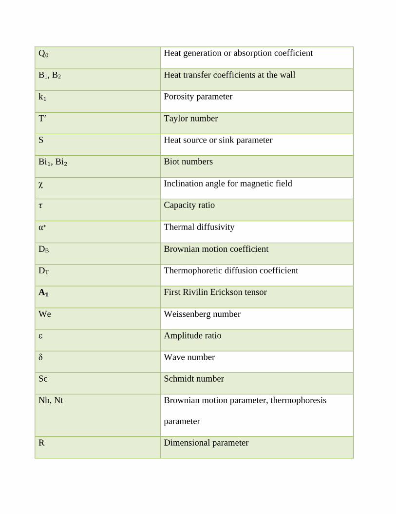
Q₀ Heat generation or absorption coefficient
B1, B2 Heat transfer coefficients at the wall
k₁ Porosity parameter
T′ Taylor number
S Heat source or sink parameter
Bi₁, Bi₂ Biot numbers
χ Inclination angle for magnetic field
𝜏 Capacity ratio
α∗ Thermal diffusivity
DB Brownian motion coefficient
DT Thermophoretic diffusion coefficient
A₁ First Rivilin Erickson tensor
We Weissenberg number
ε Amplitude ratio
δ Wave number
Sc Schmidt number
Nb, Nt Brownian motion parameter, thermophoresis
parameter
R Dimensional parameter

L, L1, L2 Diffusion coefficient parameter, Diffusion
coefficient parameters for case of homogeneous
and heterogeneous reactions
Λ Temperature difference parameter
ζ Concentration difference parameter
D Coefficient of molecular diffusion
KT Thermal diffusion ratio
Cs Concentration susceptibility
k Curvature parameter
Sr Soret number
Du Dufour number
β₁ Sisko fluid parameter
Da Darcy number
γ₁ Chemical reaction parameter
kc , ks Rate constants
C₁∗, C₂∗ Concentrations of species
H, K Strength of heterogeneous and homogeneous
reactions respectively
α₁ Prandtl fluid parameter
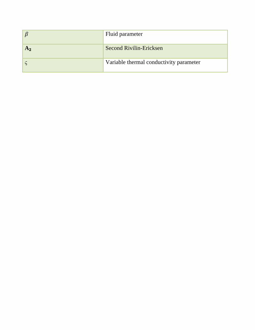
𝛽 Fluid parameter
A₂ Second Rivilin-Ericksen
ς Variable thermal conductivity parameter

Contents
1 Fundamental concepts and literature survey 6
1.1 Background . . . . . . . . . . . . . . . . . . . . . . . . . . . . . . . . . . . . . . . 6
1.2 Basic laws and fundamental equations . . . . . . . . . . . . . . . . . . . . . . . . 18
1.2.1 Mass conservative law . . . . . . . . . . . . . . . . . . . . . . . . . . . . . 18
1.2.2 Momentum conservative law . . . . . . . . . . . . . . . . . . . . . . . . . 19
1.2.3 Energy conservative law . . . . . . . . . . . . . . . . . . . . . . . . . . . . 19
1.2.4 Concentration law . . . . . . . . . . . . . . . . . . . . . . . . . . . . . . . 21
1.2.5 Compliant walls . . . . . . . . . . . . . . . . . . . . . . . . . . . . . . . . 21
2 Entropy generation in peristalsis with different shapes of nanomaterial 23
2.1 Introduction . . . . . . . . . . . . . . . . . . . . . . . . . . . . . . . . . . . . . . . 23
2.2 Flow configuration . . . . . . . . . . . . . . . . . . . . . . . . . . . . . . . . . . . 24
2.2.1 Entropy generation and viscous dissipation . . . . . . . . . . . . . . . . . 28
2.3 Solution methodology . . . . . . . . . . . . . . . . . . . . . . . . . . . . . . . . . 29
2.3.1 Zeroth order systems and solutions . . . . . . . . . . . . . . . . . . . . . . 29
2.3.2 First order systems and solutions . . . . . . . . . . . . . . . . . . . . . . . 30
2.4 Discussion . . . . . . . . . . . . . . . . . . . . . . . . . . . . . . . . . . . . . . . . 31
2.5 Conclusions . . . . . . . . . . . . . . . . . . . . . . . . . . . . . . . . . . . . . . . 45
3 Investigation of entropy generation in peristalsis of magneto-nanofluid with
second order slip conditions 46
3.1 Introduction . . . . . . . . . . . . . . . . . . . . . . . . . . . . . . . . . . . . . . . 46
3.2 Flow Configuration . . . . . . . . . . . . . . . . . . . . . . . . . . . . . . . . . . . 46
1

3.2.1 Entropy generation and viscous dissipation . . . . . . . . . . . . . . . . . 50
3.3 Solution methodology . . . . . . . . . . . . . . . . . . . . . . . . . . . . . . . . . 51
3.3.1 Zeroth order systems and solutions . . . . . . . . . . . . . . . . . . . . . . 51
3.3.2 First order systems and solutions . . . . . . . . . . . . . . . . . . . . . . . 51
3.4 Discussion . . . . . . . . . . . . . . . . . . . . . . . . . . . . . . . . . . . . . . . . 52
3.4.1 Analysis of velocity . . . . . . . . . . . . . . . . . . . . . . . . . . . . . . . 52
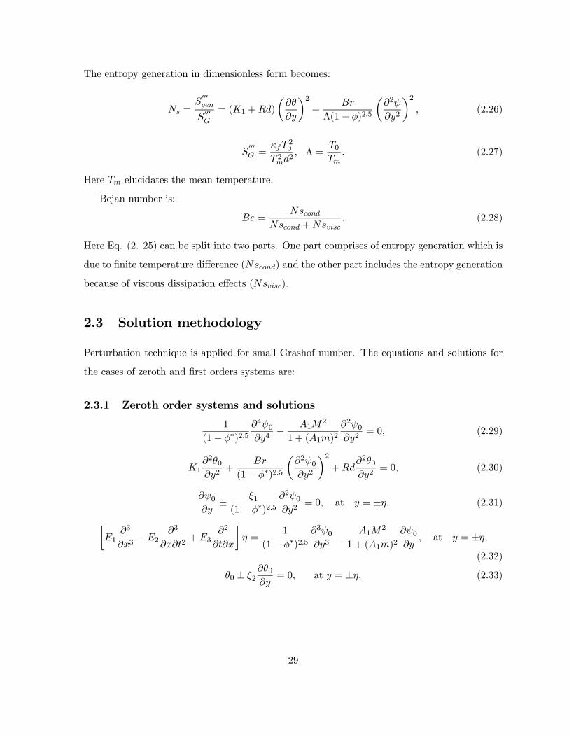
3.4.2 Analysis of temperature . . . . . . . . . . . . . . . . . . . . . . . . . . . . 55
3.4.3 Analysis of entropy generation and Bejan number . . . . . . . . . . . . . 58
3.4.4 Streamlines . . . . . . . . . . . . . . . . . . . . . . . . . . . . . . . . . . . 61
3.5 Conclusions . . . . . . . . . . . . . . . . . . . . . . . . . . . . . . . . . . . . . . . 67
4 Modeling and analysis of peristalsis of hybrid nanofluid with entropy gener-
ation 68
4.1 Introduction . . . . . . . . . . . . . . . . . . . . . . . . . . . . . . . . . . . . . . . 68
4.2 Problem modeling . . . . . . . . . . . . . . . . . . . . . . . . . . . . . . . . . . . 69
4.2.1 Entropy generation . . . . . . . . . . . . . . . . . . . . . . . . . . . . . . . 73
4.3 Analysis . . . . . . . . . . . . . . . . . . . . . . . . . . . . . . . . . . . . . . . . . 74
4.3.1 Velocity . . . . . . . . . . . . . . . . . . . . . . . . . . . . . . . . . . . . . 74
4.3.2 Temperature . . . . . . . . . . . . . . . . . . . . . . . . . . . . . . . . . . 79
4.3.3 Entropy generation analysis . . . . . . . . . . . . . . . . . . . . . . . . . . 84
4.3.4 Heat transfer rate . . . . . . . . . . . . . . . . . . . . . . . . . . . . . . . 86
4.3.5 Streamlines . . . . . . . . . . . . . . . . . . . . . . . . . . . . . . . . . . . 91
4.4 Conclusions . . . . . . . . . . . . . . . . . . . . . . . . . . . . . . . . . . . . . . . 95
5 Entropy generation in peristaltic flow of Williamson nanofluid 96
5.1 Introduction . . . . . . . . . . . . . . . . . . . . . . . . . . . . . . . . . . . . . . . 96
5.2 Formulation . . . . . . . . . . . . . . . . . . . . . . . . . . . . . . . . . . . . . . . 96
5.2.1 Determination of Entropy generation . . . . . . . . . . . . . . . . . . . . . 102
5.3 Analysis . . . . . . . . . . . . . . . . . . . . . . . . . . . . . . . . . . . . . . . . . 103
5.3.1 Velocity . . . . . . . . . . . . . . . . . . . . . . . . . . . . . . . . . . . . . 103
5.3.2 Temperature . . . . . . . . . . . . . . . . . . . . . . . . . . . . . . . . . . 105
2

5.3.3 Concentration . . . . . . . . . . . . . . . . . . . . . . . . . . . . . . . . . . 107
5.3.4 Heat transfer coefficient . . . . . . . . . . . . . . . . . . . . . . . . . . . . 109
5.3.5 Entropy generation . . . . . . . . . . . . . . . . . . . . . . . . . . . . . . . 110
5.3.6 Validation of problem . . . . . . . . . . . . . . . . . . . . . . . . . . . . . 111
5.4 Conclusions . . . . . . . . . . . . . . . . . . . . . . . . . . . . . . . . . . . . . . . 112
6 Effects of radial magnetic field and entropy on peristalsis of Williamson fluid
in curved channel 113
6.1 Introduction . . . . . . . . . . . . . . . . . . . . . . . . . . . . . . . . . . . . . . . 113
6.2 Modeling . . . . . . . . . . . . . . . . . . . . . . . . . . . . . . . . . . . . . . . . 114
6.3 Solution methodology . . . . . . . . . . . . . . . . . . . . . . . . . . . . . . . . . 120
6.3.1 Zeroth order solutions . . . . . . . . . . . . . . . . . . . . . . . . . . . . . 121
6.3.2 First order solutions . . . . . . . . . . . . . . . . . . . . . . . . . . . . . . 122
6.3.3 Entropy analysis . . . . . . . . . . . . . . . . . . . . . . . . . . . . . . . . 124
6.4 Analysis . . . . . . . . . . . . . . . . . . . . . . . . . . . . . . . . . . . . . . . . . 124
6.4.1 Validation of the Problem . . . . . . . . . . . . . . . . . . . . . . . . . . . 137
6.5 Conclusions . . . . . . . . . . . . . . . . . . . . . . . . . . . . . . . . . . . . . . . 138
7 Numerical study for peristalsis of Sisko nanomaterials with entropy genera-
tion 139
7.1 Introduction . . . . . . . . . . . . . . . . . . . . . . . . . . . . . . . . . . . . . . . 139
7.2 Problem formulation . . . . . . . . . . . . . . . . . . . . . . . . . . . . . . . . . . 140
7.2.1 Expression for entropy generation . . . . . . . . . . . . . . . . . . . . . . 145
7.3 Analysis . . . . . . . . . . . . . . . . . . . . . . . . . . . . . . . . . . . . . . . . . 146
7.3.1 Velocity . . . . . . . . . . . . . . . . . . . . . . . . . . . . . . . . . . . . . 146
7.3.2 Temperature . . . . . . . . . . . . . . . . . . . . . . . . . . . . . . . . . . 148
7.3.3 Nanoparticle concentration . . . . . . . . . . . . . . . . . . . . . . . . . . 152
7.3.4 Entropy generation analysis . . . . . . . . . . . . . . . . . . . . . . . . . . 154
7.3.5 Heat transfer coefficient . . . . . . . . . . . . . . . . . . . . . . . . . . . . 158
7.3.6 Trapping . . . . . . . . . . . . . . . . . . . . . . . . . . . . . . . . . . . . 160
7.3.7 Validation of problem . . . . . . . . . . . . . . . . . . . . . . . . . . . . . 164
3

7.4 Conclusions . . . . . . . . . . . . . . . . . . . . . . . . . . . . . . . . . . . . . . . 164
8 Entropy generation and endoscopic effects on peristalsis with modified Darcy’s
law 166
8.1 Introduction . . . . . . . . . . . . . . . . . . . . . . . . . . . . . . . . . . . . . . . 166
8.2 Modeling . . . . . . . . . . . . . . . . . . . . . . . . . . . . . . . . . . . . . . . . 167
8.2.1 Entropy generation . . . . . . . . . . . . . . . . . . . . . . . . . . . . . . . 172
8.3 Solution methodology . . . . . . . . . . . . . . . . . . . . . . . . . . . . . . . . . 172
8.4 Analysis . . . . . . . . . . . . . . . . . . . . . . . . . . . . . . . . . . . . . . . . . 173
8.5 Conclusions . . . . . . . . . . . . . . . . . . . . . . . . . . . . . . . . . . . . . . . 182
9 Entropy optimization for peristalsis of Rabinowitsch nanomaterial 183
9.1 Introduction . . . . . . . . . . . . . . . . . . . . . . . . . . . . . . . . . . . . . . . 183
9.2 Problem formulation . . . . . . . . . . . . . . . . . . . . . . . . . . . . . . . . . . 184
9.2.1 Solution of the problem . . . . . . . . . . . . . . . . . . . . . . . . . . . . 188
9.2.2 Expression for entropy generation . . . . . . . . . . . . . . . . . . . . . . 188
9.3 Analysis . . . . . . . . . . . . . . . . . . . . . . . . . . . . . . . . . . . . . . . . . 189
9.3.1 Velocity . . . . . . . . . . . . . . . . . . . . . . . . . . . . . . . . . . . . . 189
9.3.2 Temperature . . . . . . . . . . . . . . . . . . . . . . . . . . . . . . . . . . 191
9.3.3 Concentration field . . . . . . . . . . . . . . . . . . . . . . . . . . . . . . . 195
9.3.4 Entropy generation analysis . . . . . . . . . . . . . . . . . . . . . . . . . . 198
9.3.5 Heat transfer coefficient . . . . . . . . . . . . . . . . . . . . . . . . . . . . 200
9.4 Conclusions . . . . . . . . . . . . . . . . . . . . . . . . . . . . . . . . . . . . . . . 202
10 Entropy analysis in peristalsis with homogeneous-heterogeneous reaction 203
10.1 Introduction . . . . . . . . . . . . . . . . . . . . . . . . . . . . . . . . . . . . . . . 203
10.2 Problem formulation . . . . . . . . . . . . . . . . . . . . . . . . . . . . . . . . . . 203
10.2.1 Entropy generation . . . . . . . . . . . . . . . . . . . . . . . . . . . . . . . 209
10.3 Analysis . . . . . . . . . . . . . . . . . . . . . . . . . . . . . . . . . . . . . . . . . 210
10.3.1 Validation of problem: . . . . . . . . . . . . . . . . . . . . . . . . . . . . . 223
10.4 Conclusions . . . . . . . . . . . . . . . . . . . . . . . . . . . . . . . . . . . . . . . 223
4

11 Entropy analysis for the peristaltic flow of third grade fluid with variable
thermal conductivity 225
11.1 Introduction . . . . . . . . . . . . . . . . . . . . . . . . . . . . . . . . . . . . . . . 225
11.2 Modeling . . . . . . . . . . . . . . . . . . . . . . . . . . . . . . . . . . . . . . . . 225
11.2.1 Entropy generation . . . . . . . . . . . . . . . . . . . . . . . . . . . . . . . 230
11.3 Analysis . . . . . . . . . . . . . . . . . . . . . . . . . . . . . . . . . . . . . . . . . 230
11.3.1 Velocity . . . . . . . . . . . . . . . . . . . . . . . . . . . . . . . . . . . . . 230
11.3.2 Temperature . . . . . . . . . . . . . . . . . . . . . . . . . . . . . . . . . . 233
11.3.3 Entropy analysis . . . . . . . . . . . . . . . . . . . . . . . . . . . . . . . . 236
11.3.4 Heat transfer coefficient . . . . . . . . . . . . . . . . . . . . . . . . . . . . 238
11.3.5 Trapping . . . . . . . . . . . . . . . . . . . . . . . . . . . . . . . . . . . . 240
11.4 Conclusions . . . . . . . . . . . . . . . . . . . . . . . . . . . . . . . . . . . . . . . 242
5

Chapter 1
Fundamental concepts and literature
survey
Here our aim is to provide the background about some relevant concepts utilized in the sub-
sequent chapters. This includes the concepts of peristalsis, entropy, nanofluid and some basic
law and equations related to fluid flow.
1.1 Background
The word peristalsis is originated from the Greek word “peristaltikos” which means “clasping
and compressing”. This type of motility is responsible for transportation among different parts
of body. In this mechanism the material is propelled through the progressive waves consisting
of contraction and expansion (as first presented by Bayliss and Starling [1]) and this helps in
movement of the material. These waves may be short or long in length. It is based on the
involuntary characteristic of the smooth muscles that are involved in peristalsis. Hence this
mechanism cannot be controlled by someone by choice but smooth muscles works when they
are stimulated to do so. This motility is very useful in digestion and some other situations
witnessed in physiology.
In living beings this activity is found in transport of food particle through esophagus, chyme
movement in stomach, urine transport from kidney, movements involved in the small and large
intestines, vasomotion of blood vessels, bile movement in duct, spermatic movement, ovum
6

movement in fallopian tube etc. This activity is initiated in the human beings when any food
stuff is chewed and swallowed through the esophagus. At this stage the peristaltic wave start
from the upper position of tube and propagate along the complete length and transfer this food
to stomach and here epiglottis also helps to route this bolus into esophagus instead of entering
this into windpipe. This is also termed as esophageal peristalsis. Afterwards this chewed food
stuff is churns through peristalsis and mix it with gastric juices. The gastric juices help to
dissolve this food through chemical and mechanical actions. At last after few hours this food
becomes the chyme which is the semi-solid like mixture. Then through peristalsis this material
is forced to small intestine where nutrients are absorbed through intestinal walls into blood
streams. At last final absorption took place in large intestine when peristalsis carried this
material to large intestine where waste material also eliminated through it.
Reverse peristalsis also occurs in cub- chewing animals including cows, sheep, camels etc.
where chewed material is brought back to mouth for chewing again. In human beings the
reverse peristalsis does not occur normally. This happens under certain circumstance like food
poisoning that caused disturbance in stomach and activate the emetic centre of brain that
results in immediate vomiting.
Beside the contribution of peristalsis in living organisms, this activity is involved in many
industrial, engineering and biomedical applications. At industrial level this activity is adopted
for the transportation of toxic liquid, sanitary fluid transport etc. It is also employed in the
transportation of nuclear waste material. It is also used in pumping phenomenon like roller
pumps, finger and hose pumps etc. Moreover these pumps are utilized in mining and metallurgy,
food and beverage, biopharmaceutical etc. Heart lung machine, dialysis machine and endoscopy
also involve peristalsis.
Due to such applicability of the topic in the field of physiology, medical devices, industrial
applications persuaded the mathematicians, physicists and engineers to investigate more in
this arena. The myogenic theory of peristalsis goes back to Engelmann [2] who investigated
this activity in ureter. He concluded that there is no ganglias in the muscular layer but few
at the end of the ureter. Afterward some initial attempts were endeavored by Lapides [3]
and Boyarsky [4]. They studied the physiology of human ureter. The significance behind any
mathematical modeling of physiological fluid flows is to get a better understanding for the
7

specific flow that is being modeled. As the peristaltic flow is evident in mostly physiological
situations so the precise mathematical analysis may help to study the flow in human body.
Latham [5] did the pioneer work on peristalsis. He considered the viscous fluid for study of
peristalsis in ureter. He compared the experimental results with theoretical research. These
are found in good comparison. After him Shapiro et al. [6] did the study for peristalsis in two-
dimensional channel. They examined the series of waves in inertia free flow by adopting the
long wavelength and small Reynolds number approach. Theoretical results are also validated
experimentally for axisymmetric and plane configurations. Burns and Parkes [7] analyzed the
peristalsis in view of lubrication approach. They obtained the series solution. Their model
was best suited for creeping flow as they have neglected the inertial terms from Navier-Stokes
equations. Barton and Raynor [8] accounted the peristaltic activity in tubes for the study
of movement of chyme to small intestine. Fung and Yih [9] and Hanin [10] also analyzed
peristalsis. Peristaltic activity in circular shape cylindrical tubes is investigated by Yin and
Fung [11], Li [12] and Chow [13]. They have considered the viscous fluid. Li [12] gave a
comparison for axisymmetric and two-dimensional channel by obtaining a series solution. Chow
[13] also analyzed the axisymmetric flow by series solution. Here the flow is induced by Hagen-
Poiseuille flow. Meginniss [14] discussed the peristalsis in a roller pump tube in presence of
low Reynolds number. Lykoudis and Roos [15] studied the peristaltic flow in ureter. They
have utilized the lubrication approximation. Zien and Ostrach [16] also applied the lubrication
theory to their problem by considering viscous, two-dimensional and incompressible fluid. At
zero mean volume flow rate inertial effects in Navier-Stokes equations has been studied. They
declared that their model is appropriate for the case of ureter. Results for peristalsis in view
of experimental and theoretical sense are also validated by Yin [17], Eckstein [18], Weinberg
[19] and Yin and Fung [20]. Weinberg [19] mentioned that his results are in good comparison
with ureteral analysis. Weinberg et al. [21] studied the impacts on ureter by imposing different
waves. Jaffrin and Shapiro [22, 23] investigated the pumping and reflux in peristalsis. Lew
et al. [24] investigated flow in the small intestine. Circular cylindrical axisymmetric tube
has been taken for the analysis. They obtained two series form solution. One for the case
of peristalsis compression without net fluid transport and other when peristalsis generated
deprived of net pressure gradient. Lew and Fung [25] collaborated for work on peristalsis in
8

valve vessels for small Reynolds number. Fung [26] examined the peristaltic wave in ureter by
evaluating the muscles action. He considered the tissues elasticity as exponential type. Hill
modified equations were utilized for muscles. Flow was considered axisymmetric having the
small wavelength. Peristalsis in a tube by utilizing the finite-element technique is examined by
Tong and Vawter [27]. Jaffrin [28] examined the peristaltic transport in inertial system. He
accounted the streamline curvature effects. His investigation can be applied to roller pumps
and alimentary canal. Peristaltic activity by using the Frobenius techniques in two-dimensional
geometry is examined by Mitra and Parasad [29]. Negrin et al. [30], Manton [31], Gupta and
Seshadri [32] and Liron [33] also put forward their attempts. In this regard, Brown and Hung
[34] also executed the study on experimental and computational bases. In another study [35]
they have solved the Navier stokes equations numerically in curvilinear coordinates. Kaimal
[36] and Bestman [37] dealt with this activity by utilizing long wavelength strategy. Rath [38]
planned the study for lobe shape tube. Results for pressure flow and velocity are calculated
and compared. Some other studies from literature can be referred through studies [39-50].
Until now, we have given the attention to discuss the literature on the peristalsis of viscous
fluid. However in real life problems, all the fluids do not exhibit the viscous fluid characteristics
(direct and linear relationship between shear stress and deformation rate). Mostly natural phe-
nomenon witnessed the involvement of non-Newtonian fluids. As peristalsis is found extensively
in human body, where we observed that the chewable food, blood, chyme etc. all lie in the
category of non-Newtonian fluids. Besides these, different oils, ketchup, lubricants, shampoo,
toothpaste, honey, custard, muds, paints, polymer solutions, industrial materials etc. all behave
as non-Newtonian fluids. All the non-Newtonian fluids depend on their rheological properties.
Hence these cannot be mathematically modelled through single constitutive relation. Differ-
ent models has been presented ([51, 52]) and utilized by the researchers depending on the fluid
characteristics. Raju and Devanathan [53] provided their first attempt for power law fluid. This
fluid model describes the pseudoplastic, dilatant and Newtonian fluid for changing the values of
power law index. They treat the blood as pseudoplastic fluid during the flow in axisymmetric
tube. Becker [54] gave a detailed description of different non-Newtonian fluids. He also exam-
ined different types of flow problems. Deiber and Schowalter [55] investigated the peristalsis of
viscoelastic material in a tube. They also accounted the porous medium. Viscoelastic materials
9

are also employed by Bohme and Friedrich [56] in planar channel. They investigated the inertia
free fluid subject to lubrication approach. Approximate solutions are obtained up to second
order of approximation for amplitude ratio. Pressure discharge and pumping efficiency were the
focus of their study. Micropolar fluid is also attended by Devi and Devanathan [57]. Pressure
gradient and micro-rotation is examined. Srivastava and Srivastava [58] look for the peristalsis
of Casson fluid. They considered blood as two-layer suspension of Casson fluid and peripheral
layer of plasma. Results were compared with studies for without peripheral layer. Investigation
for second order fluid flow in a tube is due to Siddiqui and Schwarz [59]. They deduced their
results for the special case of axisymmetric Newtonian fluid. Misra and Pandey [60, 61] talked
about the non-Newtonian fluids by utilizing the power law fluid model as food bolus in one of
their studies for esophagus. Mernone et al. [62] attended the Casson fluid model and calculated
the perturbation solutions. Herschel-Bulkley model has been explored by Vajravelu et al. [63].
Trapping and pressure rise were also investigated. Hayat and Ali [64, 65] scrutinized the third
grade and power law models for peristalsis. Horoun [66, 67] designed the analysis for third and
fourth grade fluids by taking the asymmetric and inclined asymmetric geometries respectively.
Reddy et al. [68] examined the power law model for asymmetric peristalsis. They considered
the waves traveling with different amplitudes for asymmetry in geometry. Hayat et al. employed
different fluid models (Burger [69], micropolar [70], Carreau [71]) for peristalsis by moderating
different flow assumptions. Wang et al. [72] attended Sisko model. This predicts the shear
thinning and shear thickening effects for different values of power law index. Mekheimer and
Elmaboud [73] carried out the study for couple stress fluid. They modelled the study in an
annulus. Frictional forces, pressure rise and trapping were focused. They emphasized on the ap-
plication of endoscope. Hariharana et al. [74] presented an investigation for Burger and power
law models in a tube. They employed the different wave forms including square, trapezoidal,
multi sinusoidal and sinusoidal. They utilized the Fourier series in their analyses. Path lines
were also drawn to investigate the reflux. Muthu et al. [75] discussed micropolar model for fluid
in a tube. Hayat et al. [76, 77] continued to extend the literature by attaining the attempts
for Maxwell and Johnson-Segalman models. Tripathi et al. [78] focused on viscoelastic mate-
rials by employing the fractional Maxwell technique. Hayat et al. [79] studied the third grade
fluid in curved geometry. They analyzed the heat and mass transfer. Third grade fluid is the
10

differential type fluid. This model describes the shear thinning, shear thickening and normal
stresses. Alsaedi et al. [80] addressed the Prandtl fluid to examine peristalsis. Convection
transfer of heat has been also investigated. Hayat et al. [81] examined the Eyring Powell fluid
with convection on the boundary. Chemical reaction has been also carried out. This model
predicts the results accurately at high and low shear rates. Some studies reported by Hayat
et al. [82, 83, 84, 85] on non-Newtonian fluids are also useful. Here the authors have utilized
the Soret, Dufour, radial magnetic field, rotation effects. Sadaf and Noreen [86] carried out the
investigation for Rabinowitch fluid. Rabinowitch model describes the viscous, shear thinning
and shear thickening effects.
Amelioration of heat transfer capability is the need of time and required in every field. It is
primary apprehensions for scientist nowadays. Peristalsis with heat transfer effects is necessary
from the biomedical point of view. Whenever a process runs it involves heat loss. From the
past era there is much more interest found in the field of nanotechnology. The reason behind
this is the enhancement in heat transfer efficiency. Nanofluid are the new class of advanced
heat transfer fluid that are homogeneous mixture of base fluid and suspended particles in it.
These are not just prepared by mixing the nanoparticles in host fluids but involve the chemical
processes. Utilizing the nanoparticles of millimeter or micro size caused eventual sedimentation
and corrosion. Hence nano size particles (1-100 nm) are used. This will helps to minimize the
gravitational effects and enhances the stability of mixture. For nanofluid the contact surface
area is greater when compared with microparticles. This will cause quick thermal response
and hence enhances the heat transfer. Size, material and shape of the particles are the main
factor that effected the thermophysical properties of nanofluid. With same volume fraction of
different nanoparticles, the efficiency of nanoliquids can be different. Different nanoparticles
ceramics (Alumina, Silicon carbide etc.), metals (Aluminium, copper etc.) Carbon (Graphene
etc.) are utilized in traditional liquids i.e. water, oils etc. Choi [87] gave the name “nanofluid”
to this material. Nanoliquids are used for cooling purposes like cooling in automotive engine,
solar energy, refrigeration, electronic cooling, drug delivery, aerospace, cooling and heating of
buildings, oil recovery, desalination, lubrication, drilling, nuclear cooling, boiler etc. These new
fluids have enhanced thermal properties when compared with traditional liquids. Due to its
stability and little settling the nanofluids are found more proficient. Besides the industrial and
11

engineering applicability, the nanoliquids are also being used in biomedical field. Iron based
nano materials are utilized as delivery vehicle up the blood stream to tumor. This will help to
deliver the drugs in cancer patients. Nanoporous membranes with help of Ultraviolet source
can kill the virus and bacteria from water. Due to such ample novelty the different models
are used by the researchers. Maxwell [88] model for spherical shaped particles, Hamilton and
Crosser [89] for different shapes of nanomaterial, Xue [90] for nanotubes particles are important
to mention here. In these models the characteristics of fluid and particles are separately pro-
vided. Buongiorno [91] model was based on seven slip mechanisms for convective transport. He
proposed that among these only Brownian motion and thermophoresis are prominent. Birkman
[92] gave the model for viscosity of the nanofluids. Khanafer and Vafai [93] provided a critical
synthesis for the nanoliquids characteristics. Sheikholeslami et al. [94-96] developed analyses
in presence of MHD and radiation for different conditions. Shehzad et al. [97] addressed the
peristaltic flow of nanofluid in presence of Joule heating. Abbasi et al. [98] reported the effect
of spherical and cylindrical particles. Bhatti et al. [99] addressed the Sisko fluid treating it
as blood and Titanium nanoparticles for endoscope application. Sayed et al. [100] examined
the non-Newtonian nanofluid in an inclined asymmetric geometry. Some more attempts can be
highlighted via refs. [101-110]. The utilization of hybrid nanofluid can be seen through refs.
[111-115].
Magnetohydrodynamics is the study of dynamics of fluids when magnetic field is involved.
It is the property of electrical conducting fluid that it become polarized and change the MHD
itself. This property has significant importance and note worthy applications in the field of
biomedical engineering. As blood behaves as the conducting fluid so this characteristic of blood
has been considered in certain clinical applications. MHD is applied to reduce the bleeding in
case of severe injuries. As magnetic field slows down the flow. This property is also accounted in
surgical operation to drop blood flow. Magnetic resonance imaging (MRI) has been employing
for diagnosis purposes. Further it is found for cancer treatment [116] method to guide the iron-
based nanomaterials. Super paramagnetic iron oxide nanoparticles are found proficient for drug
delivery. Trapping phenomenon may cause thrombus in blood vessels that can be disappeared
with the help of MHD. Its applicability can also be seen in hyperthermia [117], intestinal
disorders and magnetic endoscopy. Industrial processes may include solar power technique,
12
remote sensing to screen the non-proliferation, geothermal extractions, signal processing, power
generation processes, MHDs sensors etc. In natural phenomenon like Earth magnetic field to
solar wind, magnetic field of stars and planets this activity is also observed. During MHD
another physical aspect has been also inspected named as Joule heating, which occurs as a
result of implication of magnetohydrodynamic aspect. The result of current through conductor
produces heating. Many common applications are working on this principle, like hair dryer,
electric heater, iron to remove wrinkle etc. Different researches have been carried out on the
concept of magnetohydrodynamics. Magnetic field during blood pumping has been studied by
Stud et al. [118]. Shehawey and Husseny [119] presented a study of peristalsis by employing
magneto fluid. Perturbation solution has been constructed in presence of porous boundaries.
Mekheimer [120] studied the blood flow in non-uniform channel. Naby et al. [121] examined
the trapping in presence of MHD. Eldabe et al. [122] analyzed bioviscosity fluid for MHD
characteristics. Hayat and Ali [123] also investigated hydrodynamic flow. In another analysis
Hayat et al. [124] covered the endoscope problem for Jeffrey fluid by employing magnetic
field. Ebaid [125] carried out a numerical analysis for MHD peristalsis of biofluid with varying
viscosity. Some more attempts here can be viewed (refs. [126-131]). It is also observed that
Hall current cannot be ignored for situations associated with strong magnetic field (see refs.
[132-139]).
In natural phenomenon chemical reactions also takes place. It may be of constructive or
destructive type which depend on the nature of reactants that take part in chemical reaction.
These reactions are homogeneous if the reactants are in same state otherwise named as het-
erogeneous reaction, which are of keen importance in medical field because of production of
biodiversity. In peristalsis there are many processes where chemical reaction clearly involved,
named as metabolism. During some reactions, the energy released is used by cell to proceed life
e.g. during the breakdown of glucose, while for later energy is absorbed including the process of
formation of protein. Catalytic reactions are also observed in living beings. Basically, catalyst
is an agent that enhances the speed of reaction. In living organisms, enzymes play the role as
catalyst. Without these enzymes the process of metabolisms is too slow that it will take even
centuries to complete, hence there is no chance of survival. As temperature and concentration
of the reactants is less to react itself. Enzymes helps to reduce the activation energy required.
13

There are different enzymes each worked with a particular substrate. Missing enzymes may
lead to metabolic disorders. Beside these applicability catalysis converter has been utilized
to produce Ammonia. Fog formation, batteries, production of polymer, electrolytic cells, hy-
drometallurgical industry witnessed some applicability of chemical reaction. Initial studies on
homogeneous-heterogeneous reactions [140, 141] have been reported by Merkin and Chaudhary
and Merkin respectively. Merkin investigated the first order heterogeneous and cubic auto-
catalytic homogeneous reaction. Further Hayat et al. [142, 143] put forward their analysis for
chemical reaction, convective conditions and Hall effects. Awais et al. [144] commenced a study
for chemical reactions in tapered channel by using two phase nanoliquids. They have utilized
the silver and copper nanomaterial. More relevant studies in this direction can be seen via
studies [145-149].
Porous material is characterized as having voids or pores in it. Many natural materials like
soil rocks, zeolites, ceramics and cements, biological materials such as bones, cork, capillaries,
filters etc. witnessed the examples of porous materials. This concept is utilized in different
engineering branches such as petroleum engineering, construction engineering, geoscience, ma-
terial science, biophysics, biology etc. Fluid flow via porous medium has gained a lot of interest
and importance and it becomes a separate branch. Fluid flow from porous media is influenced
by certain properties of media, tensile strength, permeability, porosity etc. Experimental work
on flow via porous medium is experienced by Darcy [150]. Classical Darcy law works well for
viscous flow. Simple relation between pressure gradient and flow rate is elucidated through this
relation. These postulates are valid for the flow in tubes, capillaries and some other applica-
tions in earth sciences. For non-Newtonian fluids the modified Darcy law preserves the surface
tension force. Johansen and Dunning [151] commenced a study for capillary system by focus-
ing on wettability. Affifi and Gad [152] reported a study on porous medium for pulsatile fluid
peristalsis. Rao and Mishra [153, 154] examined the porous medium for peristalsis. They [153]
employed porous tube filled with power law fluid. In another study [154] porous peripheral layer
for gastrointestinal tract has been investigated. Elshehawey et al. [155] canvassed the study for
peristalsis in tapered pore by considering viscous fluid. They considered the compressible fluid.
They deduced the fact that induced net flow is strongerly influenced by liquid compressibility.
Tan and Masuoka [156, 157] reported their studies for porous medium by using second grade
14

and Oldroyd-B-fluid. They analyzed the Stoke’s first problem. Vajravela et al. [158] attended
peristalsis in porous annulus. By commencing the studies for porous medium Hayat et al.
[159, 160] accounted the effects of Hall and rotation in peristalsis of Oldroyd-B-fluid and Stokes
first problems for third grade fluid. Further studies [161-164] also gave a look on literature for
highlighting the novelty of porous space.
For fluid flow problems there are two main boundary conditions namely no-slip and slip
boundary conditions. No-slip condition has been validated through theory for viscous fluids
according to which the fluid will adhere to wall and there in no relative velocity among them.
Moreover, shear stress arises due to distortion of fluid particles. However, for certain conditions
such as fluid flow in capillary vessels, polymer melts extrusion etc. where no-slip conditions
are no more valid. In human body where flow also dissatisfied the no-slip conditions, slip
conditions are adopted. This technique is significant to polish the artificial heart valve, polymer
industry, paints etc. In slip there is direct relation between velocity and shear stress of the
fluid. Depending upon the fluid’s nature, slipping of fluid at the wall varies. Hayat et al.
[165] presented the study for peristalsis in porous medium. They have chosen the partial slip
conditions on boundary. Adomian decomposition technique has been used to find solution.
Trapping and pumping have been also discussed. Ali et al. [166] also encountered the problem
for peristalsis with slip conditions, MHD and variable viscosity. Series solution have been
developed in this case. Ebaid [167] captured the effects for slip conditions in presence of MHD in
an asymmetric geometry. Srinivas et al. [168] also reported the slip and magnetohydrodynamics
in peristalsis. Johnson Segalman fluid model for slip conditions has been focused by Akbar et al.
[169]. Mustafa et al. [170] attended slip effects for viscous nanofluid. Sayed et al. [171] explored
the slip conditions for velocity. Tangent hyperbolic nanofluid model and copper water material
has been investigated by Hayat el al. [172, 173]. Another type of boundary conditions has also
been accounted during flow problems. These are collection of Fourier law and Newton law of
cooling. Some literature is mentioned here for view. Ramesh [174] employed the convective
conditions for couple stress fluid. He also accounted the porous media. Hayat et al. [175]
adopted the convective boundary conditions in peristalsis through curved channel. Shahzadi
and Nadeem [176] also employed these conditions for metallic nanoparticles.
Compliance as medical terminology is defined as the capability of vessel to bulged as a
15

result of pressure on it and persist its original position. On other side it is related to material’s
ability to deform elastically as a result of an applied force. It is the inherent property of
capillaries, arteries, valves, veins and muscles in living organisms. This property of blood
veins is responsible for blood pressure changing. This characteristics has been appealed by
the researchers as compliant nature of surfaces cause reduction in drag force. As peristalsis
is involved in physiology and clinical applications. Therefore this property has advantages to
utilize. For mathematical modelling the compliant nature is describes in terms of elastance,
rigidity and stiffness through mathematical expressions. This will help to treat these walls as
membrane. Many studies have been conducted in this way. Mittra and Prasad [177] conducted
an initial study by adopting flexible wall. Srivastava and Srivastava [178] presented the study
by adopting the viscoelastic features of the wall geometry. Particulate phase effect has been
investigated on qualitative and quantitative basis. Elnaby and Haroun [179] also pay attention
to this effect. Javed et al. [180] addressed the study by using Burger fluid in flexible wall
channel. Jyothi et al. [181] reported the investigation on MHD Johnson fluid in complaint
wall channel. Hayat et al. [182] portrayed the study for endoscope analysis while adopting slip
and flexible walls. The studies [183, 184] examined the wall properties effects under magnetic
field and variable liquid characteristics. Javed and Naz [185] treated the realistic fluid in flow
geometry having compliance characteristics.
Heat and mass transfer always occur during the process of flow. Heat transfer modes include
conduction, convection and radiation. All these processes are involved during fluid flow. The
conduction during fluid flow has been analyzed through Fourier’s law. Convection is dominant
mode in fluids for transfer of heat. Influence of gravity in different scenario also plays significant
role. Sometimes these effects are so prominent and cannot be ignored. At horizontal surfaces
these effects are not effective to study as compared to vertical and inclined geometry involved
in laboratory and real-life situations. As a result of gravity natural convection occurs. Mixed
convection is the combination of natural and forced convection. Mixed convection activity has
been greatly carried out for heat transfer processes including process of nuclear impurities,
MHD generators, chemical plants etc. Srinivas et al. [186, 187] modeled the mixed convection
phenomenon. They have given the attention to heat and mass transfer effects and chemical
reaction in their respective studies. Hayat et al. [188] commenced a study for mixed convective
16
flow with slip boundary conditions. Assumptions of Joule heating and Soret and Dufour effects
have been modeled. Mustafa et al. [189] addressed mixed convective flow of fourth grade fluid
with Soret and Dufour effects. Water based nanoliquids in presence of mixed convection has
been studied by Hayat et al. [190]. Convective boundary conditions, Hall effects and Joule
heating have been accounted. In another study [191] they accounted the mixed convection
phenomenon in tapered asymmetric channel. Tanveer et al. [192] reported a study in view of
mixed convection effect for Eyring Powell fluid in curved configuration. Radiation is also another
mode of heat transfer nowadays applicable in many biomedical applications. All these modes
maintained a healthy temperature and remove the extra heat from body if necessary. Sweating,
vasoconstriction, vasodilation, through urine etc. are all different way of heat transfer. Heat
and mass transfer effects have gained importance due to its existence and applicability. Srinivas
and Kothandapani [193] talked about heat transfer aspect in asymmetric channel. Mekhemier
and Elmaboud [194] elaborated the heat transfer in a vertical annulus. Nadeem and Akbar [195,
196] also worked for heat transfer aspects. Further studies about this aspect can be noticed
from the refs. [197-200].
Natural activities are spontaneous, irreversible and complex. During fluid flow many processes
involve fluid friction, Joule heating, chemical reactions etc. This caused change in system’s
thermodynamics. These kinds of activities caused disorderliness in the system. Study of dis-
orderliness of the system is named as entropy. The concept of entropy goes back to Rudolf
Clausius, who defined the entropy in the thermodynamic sense. Second law of thermodynamics
is utilized for entropy. This law shows that entire actual processes are irreversible and this
irreversibility can be assessed through entropy generation analysis. Heat transfer laws and fluid
mechanics principles are combined to ascertained strategies for entropy generation optimization.
Foremost target behind the designing of different devices and system is to provide the maximum
output and to minimize the entropy. In thermodynamic sense this is related to enhance heat
transportation rate and estimating the performance of a system. To obtain the sophisticated
energy efficiency the researchers have moved to the thermodynamic approach EGM (entropy
generation minimization) in thermal engineering system and devices. This approach is quite
beneficial in designing the engineering devices. This great applicability and ample application
can be seen through its utilization in reactors [201], chillers [202], microchannels [203], air sepa-
17

rators [204], fuel cells [205], helical coils [206], evaporative cooling [207], curved pipes [208], gas
turbines [209] etc. Besides these with reference to peristalsis the study of entropy is very crucial,
as physiological processes are complex and spontaneous. From the medical point of view, it
is necessary to venture the factor that causes the greater irreversibility and find measures to
control them.
Bejan [210] employed the thermodynamics second law to estimate the irreversibility in
the processes of heat transfer. His paper comprises of two parts. Firstly he investigated the
production of irreversibility. In other part he reviewed the second law for heat exchangers in
classical engineering. He presented the analytic methods for irreversibility minimization. In
another study [211] he gave the method for EMG in thermodynamics systems. Sheikholeslami
and Ganji [212] scrutinized a study of entropy for nanofluids. Akbar [213] reported a study for
irreversibility analysis in a tube. MHD characteristics have been also accounted. Akbar et al.
[214] also paid attention to planar channel by employing water based nanoliquids. Abbass et
al. [215] presented the study for irreversibility analysis in flexible wall channel. Hayat et al.
[216, 217] studied entropy by employing single and multi-walled CNTs and Jeffrey fluid. More
studies in this area can be highlighted through [218-225]. It is noticed that the literature on
entropy analysis with reference to peristalsis is scarce yet. Researchers have started working in
this field because of its utility and novelty.
1.2 Basic laws and fundamental equations
Real situations of fluid flow can be captured through mathematical modeling in terms of physical
laws. These laws are:
1.2.1 Mass conservative law
This law witnessed the conservation of mass. For the case of no source/sink and compressible
fluid, equation of continuity is
div(V) +
= 0 (1.1)
where and V = ( ) portrayed the respective density, time and velocity field.
18

For incompressible fluid it becomes
+
+
= 0 (1.2)
For Cylindrical coordinates
+
+
= 0 (1.3)
For curved geometry we have
[( +∗)] +∗
= 0 (1.4)
1.2.2 Momentum conservative law
Equation of motion satisfies
V
= b+∇τ (1.5)
here b τ depicts the body force and Cauchy stress tensor.
τ = −I+ S (1.6)
where the pressure and S the extra stress tensor which varies for different fluid.
For two phase nanoliquids
V
= b+∇τ (1.7)
where
= (1− ∗) + ∗ (1.8)
where and are densities of nanomaterial and base liquid.
1.2.3 Energy conservative law
It is expressed in the form
= −∇q+ (1.9)
19

Here q denote heat flux, temperature and specific heat. term describes heat charac-
teristics, including viscous dissipation, radiation etc.
q = −∇ (1.10)
where elucidate the thermal conductivity.
For two phase model for nanoliquids
()
= ∇2 + (1.11)
where
() = (1− ∗)() + ∗()
=
+ (∗ − 1) − (∗ − 1)∗( − )
+ (∗ − 1) + ∗( − ) (1.12)
Here subscript and represent the notation for nano solid material and base liquid and ∗ is
shape factor.
For Buongiorno model
()
= −∇q+ ∇ (1.13)
where and highlight specific enthalpy and diffusion mass flux of nano materials. Here
q = −∇ +
= −∇− ∇ (1.14)
where , are respective mean temperature, thermophoresis and Brownian coefficients.
Inserting for q and simplifying, we get
()
= ∇2 −∇ (1.15)
20

Finally utilizing , one arrives at
()
= ∇2 + ()
∇∇
+ ()∇∇ (1.16)
1.2.4 Concentration law
Here one has
= ∇2 + (1.17)
in which denotes the source term that may be in form of chemical reaction etc.
Concentration equation for nanoparticles is
= − 1
∇ (1.18)
Utilizing the expression for we arrive at
=
∇2
+∇2 (1.19)
1.2.5 Compliant walls
Compliance is linked to capability of an objects to bulged or recoil back to its original position.
This property can be described in terms of elastance, rigidity and stiffness. Living organisms
naturally include such muscular structure through which it is more feasible to exchange nutrient,
water etc. The flexible walls is also known as Compliant walls. Mathematically we expressed
as
∗ () = − 0 (1.20)
where 0 is the pressure outside the wall due to muscles tension and ∗ the characteristics of
walls to consider them as membranes defined by
∗ = −∗ 2
2+∗
2
2+ ∗1
(1.21)
in which elastance (−∗), mass per unit area (∗) and damping (∗1) characteristics are takeninto consideration. Study of peristalsis with and without compliant characteristics are valid
21

where disturbance due to pressure is negligible. However the compliant characteristics are
more suitable in case of deformable walls.
22

Chapter 2
Entropy generation in peristalsis
with different shapes of
nanomaterial
2.1 Introduction
This chapter analyzed the peristalsis in a vertical channel by using different shapes of nanoma-
terial. The nanomaterial utilized for this purpose is silver () with water as base fluid. The
study is based on the comparison amongst different shapes of nanoparticles (bricks, cylinders
and platelets). The walls of channel are of flexible nature. Study is done in the light of long
wavelength and low Reynolds number approximations. Solution technique utilized here is per-
turbation with Grashof number as small parameter. Entropy generation analysis is also carried
out with different shapes of nanoparticles. The graphs of Bejan number, entropy generation,
velocity and temperature are drawn for the sake of comparison through considered nanoparti-
cles. Streamlines are also studied. The results lead to the fact that an increase in nanomaterial
volume fraction decays velocity and temperature of nanofluid. The Hall parameter and Hart-
man number show opposite behavior for velocity, temperature, entropy generation and Bejan
number. Highest values of temperature, Bejan number and entropy generation have been seen
for brick shaped particles and smallest for platelet shaped particles.
23
2.2 Flow configuration
Here a vertical channel of width 2 is considered. The channel walls are considered flexible.
The walls are at the positions = ±. A wave travels with speed along the walls which propelthe fluid in motion. This wave has wavelength and amplitude (see Fig. 2.1). The walls
has temperature 0 Moreover base fluid and nanoparticles are considered thermally consistent
with respect to each other. A magnetic field of strength 0 is applied in a normal direction to
flow. Induced magnetic field is ignored because of small magnetic Reynolds number.
The Lorentz force is defined as
F = J×B (2.1)
in which B = [0 0 ] and J are the applied magnetic field and current density respectively.
When Hall effects are taken into account then current density satisfies
J =
∙E+V ×B− 1
[J×B]
¸ (2.2)
Here elucidates the effective electric conductivity of nanofluid, E is used for electric field,
the velocity field V =[ ( ), ( ) 0] represents the electron charge and the number
density of free electrons. Electric field is absent and thus
J =
∙V ×B− 1
[J×B]
¸ (2.3)
The Lorentz force then takes the form as:
F =
"
2
1 + (
)2
µ−+ (
)
¶−2
1 + (
)2
µ + (
)
¶ 0
# (2.4)
The two-phase model of effective electric conductivity of nanofluid is represented below [135,
190]:
= 1 +
3(− 1)∗
(+ 2)− (
− 1)∗ (2.5)
Here and are the electric conductivity of nanomaterial and base fluid respectively and ∗
24

is used for nanoparticle volume fraction. Now we have
F =
∙1
2
1 + (1)2(−+1)
−121 + (1)2
( +1) 0
¸ (2.6)
where 1 and the Hall parameter are defined by:
=
1 = 1 +
3(− 1)∗
(+ 2)− (
− 1)∗ (2.7)
Shape of the peristaltic wall is
= ± ( ) = ±∙+ sin
2
(− )
¸ (2.8)
Fig. 2.1: Flow Configuration
The governing equations are:
+
= 0 (2.9)
25

(
+
+
) = −
+
∙2
2+
2
2
¸+( ) ( − 0)− 1
2
1 + (1)2(−1)
(2.10)
(
+
+
) = −
+
∙2
2+
2
2
¸− 1
2
1 + (1)2( +1) (2.11)
() (
+
+
) =
∙2
2+
2
2
¸+
"2
õ
¶2+
µ
¶2!
+
µ
+
¶2#−
(2.12)
Here and are used to represent the velocity components in and directions, the
temperature, the pressure, the effective density, the effective viscosity, ( )
the effective thermal expansion, () the effective heat capacity, the effective thermal
conductivity of nanofluid and (=−4∗3∗
4
) the radiative heat flux.
The expressions for () ( ) and are:
= (1− ∗) + ∗ () = (1− ∗)() + ∗()
( ) = (1− ∗) ( ) + ∗ ( ) =
(1− ∗)25
=
+ (∗ − 1) − (∗ − 1)∗( − )
+ (∗ − 1) + ∗( − ) (2.13)
Table 1 given below represents the thermophysical properties of utilized base fluid and
nanomaterial.
Table 1: Thermophysical parameters of water and nanoparticle [190]
(kg m−3) (j kg−1 K−1) ¡W m−1K−1
¢ (l/k) × 10−6
2 997.1 4179 0.613 210
10500 235 429 18.9
Shape factor and sphericity of different shapes of nanomaterial are given in Table 2 below
[106]
26

Nanomaterial shape Sphericity Shape factor
Brick 0.81 3.7
Cylinder 0.62 4.9
Platelet 0.52 5.7
The quantities in dimensionless form are given by
∗ =
∗ =
∗ =
∗ =
∗ =
∗ =
∗1 =1
∗2 =
2 ∗ =
2
Re =
=
− 0
0 Pr =
()
=2
() 0 = Pr =
( ) 02
=
r
=16∗ 303∗
=
= −
(2.14)
Here , , and are Reynolds, Prandtl, Eckert, Brinkman, Grashof and
Hartman numbers respectively. Moreover is the radiation parameter.
After invoking large wavelength and low Reynolds number assumptions [135, 190] the con-
tinuity equation is identically satisfied and others equations lead to
=
1
(1− ∗)253
3+3 − 1
2
1 + (1)2
(2.15)
= 0 (2.16)
12
2+
(1− ∗)25
µ2
2
¶2+
2
2= 0 (2.17)
3 = 1− ∗ + ∗Ã( )
( )
!
1 = + (
∗ − 1) − (∗ − 1)( − )
+ (∗ − 1) + ( − ) (2.18)
27

The velocity slip, compliant walls and thermal slip conditions are
± 1 = 0 at = ± (2.19)
∙−∗
3
3+∗
3
2+ ∗1
2
¸ =
+
−
∙
+
+
¸+( ) ( − 0)− 1
2
1+(1)2(−1)
at = ±(2.20)
± 2
= 0 at = ± (2.21)
where 1 and 2 are dimensional slip parameters for velocity and temperature respectively.
The dimensionless forms of boundary conditions are
± 1(1− ∗)25
2
2= 0 ± 2
= 0 at = ± (2.22)
∙1
3
3+2
3
2+3
2
¸ =
1
(1− ∗)253
3+3− 1
2
1 + (1)2
at = ±
(2.23)
Here 1(= −∗33 ) 2(= ∗33 ) and 3(= ∗132 ) are the flexible walls
parameters.
2.2.1 Entropy generation and viscous dissipation
Viscous dissipation effect is given by
Φ =
"2
õ
¶2+
µ
¶2!+
µ
+
¶2# (2.24)
Dimensional form of volumetric entropy generation in defined as
000 =
2
õ
¶2+
µ
¶2!+
1
2
16∗ 303∗
µ
¶2+Φ
(2.25)
28
The entropy generation in dimensionless form becomes:
=000
000
= (1 +)
µ
¶2+
Λ(1− )25
µ2
2
¶2 (2.26)
000 =
20
22 Λ =
0
(2.27)
Here elucidates the mean temperature.
Bejan number is:
=
+ (2.28)
Here Eq. (2. 25) can be split into two parts. One part comprises of entropy generation which is
due to finite temperature difference () and the other part includes the entropy generation
because of viscous dissipation effects ().
2.3 Solution methodology
Perturbation technique is applied for small Grashof number. The equations and solutions for
the cases of zeroth and first orders systems are:
2.3.1 Zeroth order systems and solutions
1
(1− ∗)25404
− 12
1 + (1)2202
= 0 (2.29)
120
2+
(1− ∗)25
µ202
¶2+
20
2= 0 (2.30)
0
± 1(1− ∗)25
202
= 0 at = ± (2.31)
∙1
3
3+2
3
2+3
2
¸ =
1
(1− ∗)25303
− 12
1 + (1)20
at = ±(2.32)
0 ± 20
= 0 at = ± (2.33)
29

The solutions expressions are
0 =
0
√1√
0+0212 (1 +21
2)
⎛⎝
2√1√
0+02121 + 2
⎞⎠12
+ 3 + 4 (2.34)
0 = −
0
−2√1√
0+0212
22+21
4√1√
0+0212
(1+212)
12 + 4122
42+ 1 + 2 (2.35)
2.3.2 First order systems and solutions
Here we have
1
(1− ∗)25414
+30
− 1
2
1 + (1)2212
= 0 (2.36)
121
2+
(1− )25
µ2202
212
¶+
21
2= 0 (2.37)
1
± 1(1− ∗)25
212
= 0 at = ± (2.38)
1
(1− ∗)25313
+30 − 12
1 + (1)21
= 0 at = ± (2.39)
1 ± 21
= 0 at = ± (2.40)
The solution expressions are
1 =1
2415225(1 +21
2)(203
−2√1√
0+0212
−22+214√1√
0+0212
(1 +212)
q0 +0
21
2 + 12321 322
32 +
80321 3(−3123 + 3
−√1√
0+0212
2(
2√1√
0+02121 +2))) +3 + 4 (2.41)
30

1 =1
(1 −22 −32 +4
2 − 3032−√1√
0+0212
5 − 12012q0 +0
21
2) + 3031
√1√
0+0212 (1 +21
2)2
(−6 + 6√122)√1
+ 12012
q0 +0
21
2)) +1 + 2 (2.42)
in which Ci0 , 0 0 0 and 0 are constants that can be evaluated through Mathe-
matica. Here 2 = 1 +
2.4 Discussion
This section includes the graphs and related analyses for different embedded parameters. This
section contains the graphs for velocity, temperature, streamlines, Bejan number and entropy
generation. Each graph gives a comparison among different shapes of nanomaterial for the per-
tinent parameter. Fig. 2.2 is drawn for the comparative study of effective thermal conductivity
of different shapes of nanomaterial when nanomaterial volume fraction varies. This Fig. clearly
indicated that effective thermal conductivity for the case of platelet shaped particle is higher
in all cases than brick and cylindrical shaped particles. The brick shaped particles have lowest
effective thermal conductivity.
Fig. 2.2: Comparison of effective thermal conductivity for different shaped nanomaterials
31

Fig. 2.3 is sketched for the case of velocity when volume fraction of nanomaterial varies. As
expected the velocity is decreased via nanoparticle volume fraction. As higher volume fraction
enhance the shear rate, which provide resistance to flow so velocity decreases. Fig. 2.4 illustrates
the Hartman number impact on velocity. Velocity is decreasing function of Hartman number.
As Lorentz force provides obstruction to fluid flow. Hence the velocity reduces. Hall parameter
influence on velocity can be seen through Fig. 2.5. It shows the increasing behavior of velocity
for Hall parameter. Same impact is obtained for velocity slip parameter and Grashof number
(see Fig. 2.6 and Fig. 2.7). Grashof number arises due to mixed convection which is also in the
favor of velocity. In nuclear reactor cooling the mixed convection is utilized to dissipate energy
when force convection not enough to do so. Wall properties behavior on velocity is increasing
for elastance parameters while there is decreasing effect for damping parameter (see Fig. 2.8).
In all the cases of velocity profile it is found through comparative study of different shaped
nanoparticles that velocity remains lowest for case of bricks shaped particles and it is highest
for cylindrical shaped particles.
Fig. 2.3 Fig. 2.4
23 versus ∗ when 1 = 002 2 = 001 3 = 001 = 01 = 02 = 02
= 10 = 10 = 50 = 01 1 = 001 2 = 001 = 05
24 versus when 1 = 002 2 = 001 3 = 001 = 01 = 02 = 02
∗ = 01 = 10 = 50 = 09 1 = 001 2 = 001 = 05
32

Fig. 2.5 Fig. 2.6
25 versus when 1 = 002 2 = 001 3 = 001 = 01 = 02 = 02
∗ = 01 = 10 = 50 = 01 1 = 001 2 = 001 = 05
26 versus 1 when 1 = 002 2 = 001 3 = 001 = 01 = 02 = 02
= 10 = 10 = 50 = 09 ∗ = 01 2 = 001 = 05
Fig. 2.7 Fig. 2.8
27 versus when 1 = 002 2 = 001 3 = 001 = 01 = 02 = 02
= 10 = 10 = 50 ∗ = 01 1 = 001 2 = 001 = 05
28 versus 1 2 3 when = 01 = 02 = 02 = 10 = 10 = 50
33

= 01 ∗ = 01 1 = 001 2 = 001 = 05
Behavior of temperature is shown through Figs. 2.9-2.14. Fig. 2.9 explained influence of
∗ on Temperature is decreasing function of volume fraction of nanomaterial. Due to similar
reason the nanofluids are utilized for coolant purposes. As higher volume fraction of nanopar-
ticles enhance the heat transfer capability, so temperature decreases. Through comparison it is
concluded that temperature distribution remains highest for bricks shaped nanoparticles and
lowest for platelets shaped nanomaterials. The results of Hall parameter and Hartman number
on the temperature are opposite (see Figs. 2.10 and 2.11). Enhancement is seen for Hall para-
meter whereas decay is noticed for Hartman number. As Hall effect facilitate the flow, so flow
with higher mean kinetic energy has greater heat loss and hence increase in temperature is no-
ticed. Similarly regarding force the flow slows and hence less heat loss through fluid movement.
Finally decay is noticed. The Grashof number and temperature slip parameter give increasing
behavior for temperature (see Fig. 2.12 and 2.13). Radiation parameter effects on temperature
is illustrated through Fig. 2.14. Decrease in temperature is noticed in this case.
Fig. 2.9 Fig. 2.10
29 versus ∗ when 1 = 002 2 = 001 3 = 001 = 01 = 02 = 02
= 10 = 10 = 50 = 01 1 = 001 2 = 001 = 05
210 versus when 1 = 002 2 = 001 3 = 001 = 01 = 02 = 02
= 10 ∗ = 02 = 50 = 01 1 = 001 2 = 001 = 05
34

Fig. 2.11 Fig. 2.12
211 versus when 1 = 002 2 = 001 3 = 001 = 01 = 02 = 02
∗ = 01 = 10 = 50 = 01 1 = 001 2 = 001 = 05
212 versus when 1 = 002 2 = 001 3 = 001 = 01 = 02 = 02
= 10 = 10 = 50 ∗ = 01 1 = 001 2 = 001 = 05
Fig. 2.13 Fig. 2.14
213 versus 2 when 1 = 002 2 = 001 3 = 001 = 01 = 02 = 02
= 10 = 10 = 50 = 01 1 = 001 ∗ = 01 = 05
214 versus when 1 = 002 2 = 001 3 = 001 = 01 = 02 = 02
35

= 10 = 10 ∗ = 01 = 50 = 01 1 = 001 2 = 001
The observation for entropy generation and Bejan number is covered here. Fig. 2.15 is
prepared for entropy generation versus ∗. In view of this Fig. decrease in entropy generation
is seen for volume fraction of the nanoparticle. As less disorderliness is noticed with small
temperature effects. Fig. 2.16 is drawn for Hartman number variation on entropy generation
and Fig. 2.17 for Hall parameter. Decay is seen for Hartman number while an enhancement
is observed for larger Hall parameter. The reason can be directly related with temperature.
Both and the ratio of to Λ have displayed the increasing behavior for entropy generation
(see Figs. 2.18 and 2.19). Fig. 2.20 is prepared for radiation parameter on entropy generation.
Entropy generation decreases for radiation parameter (). Through all graphs it is found
that brick shaped particles have higher values and platelet shaped particles have least entropy
generation.
Fig. 2.15 Fig. 2.16
215 versus ∗ when 1 = 002 2 = 001 3 = 001 = 01 = 02 = 02
= 10 = 10 Λ−1 = 10 = 01 1 = 001 2 = 001 = 05
216 versus when 1 = 002 2 = 001 3 = 001 = 01 = 02 = 02
∗ = 01 = 10 Λ−1 = 10 = 01 1 = 001 2 = 001 = 05
36

Fig. 2.17 Fig. 2.18
217 versus when 1 = 002 2 = 001 3 = 001 = 01 = 02 = 02
= 10 ∗ = 01 Λ−1 = 10 = 01 1 = 001 2 = 001 = 05
218 versus when 1 = 002 2 = 001 3 = 001 = 01 = 02 = 02
= 10 = 10 Λ−1 = 10 ∗ = 01 1 = 001 2 = 001 = 05
Fig. 2.19 Fig. 2.20
219 versus Λ−1 when 1 = 002 2 = 001 3 = 001 = 01 = 02 = 02
= 10 = 10 ∗ = 01 = 01 1 = 001 2 = 001 = 05
220 versus when 1 = 002 2 = 001 3 = 001 ∗ = 01 = 01 = 02
37

= 02 = 10 = 10 Λ−1 = 10 = 01 1 = 001 2 = 001
Bejan number observation is analyzed in this paragraph. In view of these graphical results
we have seen that decay is seen via ∗ (see Fig. 2.21) This result seems to be same here
as in the case of temperature. The Bejan number result for change in Hartman number is
observed via Fig. 2.22. This Fig. elucidates that Bejan number decreases with an enhancement
of Hartman number. Fig. 2.23 shows that Hall parameter has increasing behavior for Bejan
number. Moreover increasing impact of Bejan number is also observed for larger Grashof
number and ratio of to Λ (see Figs. 2.24 and 2.25). Fig. 2.26 is prepared for impact of
radiation parameter. The effects here are qualitatively similar to that of temperature. In all
the above mentioned graphs for Bejan number we noticed that the values for nanoliquids with
brick shape is larger than cylindrical and platelet shapes nanomaterials.
Fig. 2.21 Fig. 2.22
221 versus ∗ when 1 = 002 2 = 001 3 = 001 = 01 = 02 = 02
= 10 = 10 Λ−1 = 10 = 01 1 = 001 2 = 001 = 05
222 versus when 1 = 002 2 = 001 3 = 001 = 01 = 02 = 02
∗ = 01 = 10 Λ−1 = 10 = 01 1 = 001 2 = 001 = 05
38

Fig. 2.23 Fig. 2.24
223 versus when 1 = 002 2 = 001 3 = 001 = 01 = 02 = 02
= 10 ∗ = 01 Λ−1 = 10 = 01 1 = 001 2 = 001 = 05
224 versus when 1 = 002 2 = 001 3 = 001 = 01 = 02 = 02
= 10 = 10 Λ−1 = 10 ∗ = 01 1 = 001 2 = 001 = 05
Fig. 2.25 Fig. 2.26
225 versus Λ−1 when 1 = 002 2 = 001 3 = 001 = 01 = 02 = 02
= 10 = 10 ∗ = 01 = 01 1 = 001 2 = 001 = 05
226 versus when 1 = 002 2 = 001 3 = 001 ∗ = 01 = 01 = 02
39

= 02 = 10 = 10 Λ−1 = 10 = 01 1 = 001 2 = 001
For the sake of trapping the streamlines are prepared. Figs. 2.27 (a-c) are drawn for the sake
of shape factor . It is noted that the size of trapped bolus is lower for brick shaped than others.
Figs. 2.28 (a and b) corresponding to brick shaped, Figs. 2.28 (c and d) are constructed to
cylindrical shaped and Figs. 2.28 (e and f) to platelet shaped nanofluids for change in Hartman
number. It is noted that increase in strength of magnetic field decreases trapped bolus size.
This bolus size is smaller for the fluid containing brick shaped nanomaterials. Figs. 2.29 (a and
b) are sketched to brick shaped, Figs. 2.29 (c and d) hold to cylindrical shaped and Figs. 2.29
(e and f) to platelet shaped nanofluids have been prepared for change in Hall parameter. It is
noted that with higher Hall parameter caused decrease in the size of trapped bolus. This bolus
size is smallest for brick shaped nanomaterials.
Fig. 2.27 (a) (b)
40

(c)
227 versus ∗ when 1 = 002 2 = 001 3 = 001 = 0 = 02 ∗ = 01
= 10 = 10 = 50 = 01 = 001 = 001() ∗ = 37 () ∗ = 49 ()
∗ = 57
Fig. 2.28 (a) (b)
228 versus for nanofluid with brick shaped nanoparticles when 1 = 002
2 = 001 3 = 001 ∗ = 01 = 0 = 02 = 10 = 50 = 01 1 = 001
41

2 = 001 () = 10 () = 30
Fig. 2.28 (c) (d)
228 versus for nanofluid with cylindrical shaped nanoparticles when 1 = 002
2 = 001 3 = 001 ∗ = 01 = 0 = 02 = 10 = 50 = 01 1 = 001
2 = 001 () = 10 () = 30
Fig. 2.28 (e) (f)
228 versus for nanofluid with platelet shaped nanoparticles when 1 = 002
42

2 = 001 3 = 001 ∗ = 01 = 0 = 02 = 10 = 50 = 01 1 = 001
2 = 001 () = 10 () = 30
Fig. 2.29 (a) (b)
229 versus for nanofluid with brick shaped particles when 1 = 002 2 = 001
3 = 001 ∗ = 01 = 0 = 02 = 10 = 50 = 01 1 = 001 2 = 001 ()
= 10 () = 30
43

(c) (d)
229 versus for nanofluid with cylindrical shaped nanoparticles when 1 = 002
2 = 001 3 = 001 ∗ = 01 = 0 = 02 = 10 = 50 = 01 1 = 001
2 = 001 () = 10 () = 30
Fig. 2.29 (e) (f)
229 versus for nanofluid with platelet shaped nanoparticles when 1 = 002
44

2 = 001 3 = 001 ∗ = 01 = 0 = 02 = 10 = 50 = 01 1 = 001
2 = 001 () = 10 () = 30
2.5 Conclusions
Some key points of present study are:
• Enhancement in nanomaterial volume fraction leads to decay in velocity, temperature,entropy generation and Bejan number.
• Hall parameter and Hartman number have opposite behaviors in all cases.
• Grashof number has increasing impact in all cases.
• The behaviors for temperature, entropy generation and Bejan numbers are qualitativelysimilar.
• The temperature, Bejan number and entropy generation have highest values for brickshaped particles and smallest for platelet shaped particles.
• Size of bolus is smaller for brick shaped nanofluids than others particles.
45
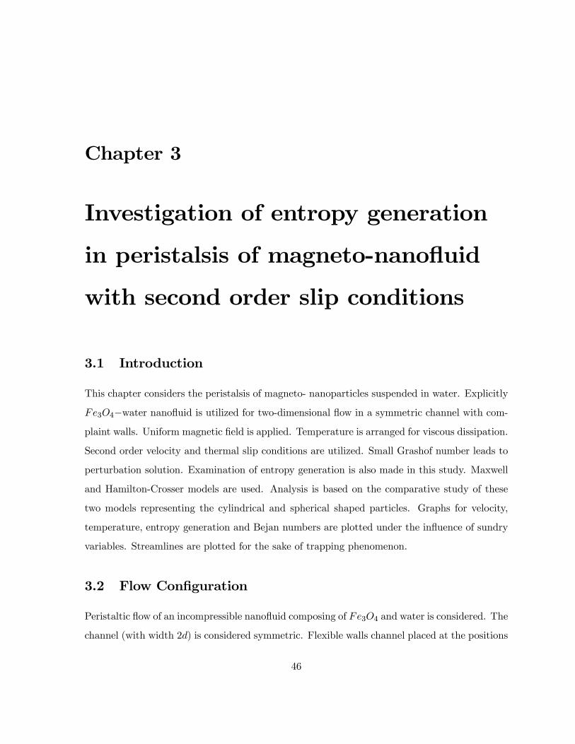
Chapter 3
Investigation of entropy generation
in peristalsis of magneto-nanofluid
with second order slip conditions
3.1 Introduction
This chapter considers the peristalsis of magneto- nanoparticles suspended in water. Explicitly
34−water nanofluid is utilized for two-dimensional flow in a symmetric channel with com-plaint walls. Uniform magnetic field is applied. Temperature is arranged for viscous dissipation.
Second order velocity and thermal slip conditions are utilized. Small Grashof number leads to
perturbation solution. Examination of entropy generation is also made in this study. Maxwell
and Hamilton-Crosser models are used. Analysis is based on the comparative study of these
two models representing the cylindrical and spherical shaped particles. Graphs for velocity,
temperature, entropy generation and Bejan numbers are plotted under the influence of sundry
variables. Streamlines are plotted for the sake of trapping phenomenon.
3.2 Flow Configuration
Peristaltic flow of an incompressible nanofluid composing of 34 and water is considered. The
channel (with width 2) is considered symmetric. Flexible walls channel placed at the positions
46

= ± where + and − denote the right and left walls respectively. The rectangular coordinatessystem is settled such as the -axis lies along the channel length where the position of the -axis
is in the direction perpendicular to the -axis. The temperature of the walls is maintained at 0
Contribution due to constant applied magnetic field is taken into account. Induced magnetic
and electric fields effects are omitted. Mixed convection and viscous dissipation are studied.
Sinusoidal waves have wavelength amplitude and speed . The shape of wave is defined by
equation given below:
= ± ( ) = ±∙+ sin
2
(− )
¸ (3.1)
Fig. 3.1: Flow Geometry
Expressions for the considered flow configuration are:
+
= 0 (3.2)
(
+
+
) = −
+
∙2
2+
2
2
¸−
2+ ( ) ( − 0) (3.3)
(
+
+
) = −
+
∙2
2+
2
2
¸ (3.4)
47

() (
+
+
) =
∙2
2+
2
2
¸+
"2
õ
¶2+
µ
¶2!
+
µ
+
¶2# (3.5)
The quantities used in the above mentioned equations are defined as: and for components
of velocity in the and directions, for effective density, the pressure, the effective
viscosity, the effective thermal conductivity, the acceleration due to gravity, ( ) ,
() and for effective thermal expansion, the effective heat capacity and the effective
thermal conductivity of nanofluids respectively. Here is used to define temperature and for
time.
The expressions of () ( ) and for the two phase models
are:
= (1− ∗) + ∗ () = (1− ∗)() + ∗()
( ) = (1− ∗)( ) + ∗( ) =
(1− ∗)25
= 1 +
3(− 1)∗
(+ 2)− (
− 1)∗
=
+ 2 − 2∗( − )
+ 2 + ∗( − )for Maxwell’s model and
=
+ (∗ − 1) − (∗ − 1)∗( − )
+ (∗ − 1) + ∗( − )for Hamilton-Crosser’s model,(3.6)
in which the symbols and in the subscript are used to represent the fluid and nanoparticles
whereas ∗ depicts volume fraction of nanoparticles. In this study two models of effective
thermal conductivity are used in above equation. The Hamilton- Crosser model is used for the
cylindrical shaped particles for ∗ = 6 whereas Maxwell model is used for spherical shaped
particles. Here ∗ represents the shape of nanoparticles. It is defined by 3Ψ where Ψ depicts
the sphericity of nanoparticles. Value Ψ = 05 is used for cylindrical shaped particles whereas
Ψ = 1 for spherical shaped particles.
Thermophysical properties of base fluid and nanoparticles are mentioned below in Table 1.
Table 1: Thermophysical parameters of water and nanoparticles
48

(kg m−3) (j kg−1 K−1) ¡W m−1K−1
¢ (l/k) × 10−6 (Ω . )−1
2 997.1 4179 0.613 210 0.05
34 5200 670 80.6 13 25000
The dimensionless quantities are introduced as:
∗ =
∗ =
∗ =
∗ =
∗ =
∗ =
∗1 =1
∗2 =
2 ∗4 =
4
2 ∗5 =
52
∗ =2
Re =
=
− 0
0 Pr =
()
=2
()0 = Pr =
( )02
=
r
=
= −
(3.7)
Here Re, Pr , and denote the Reynolds, Prandtl, Eckert, Brinkman, Hartman
and Grashof numbers respectively.
After long wavelength and small Reynolds number assumptions one has
=
1
(1− ∗)253
3+3 −21
(3.8)
= 0 (3.9)
12
2+
(1− ∗)25
µ2
2
¶2= 0 (3.10)
1 = 1 +3(
− 1)∗
(+ 2)− (
− 1)∗ 3 = 1− ∗ + ∗
Ã()
()
!
1 = + 2 − 2∗( − )
+ 2 + ∗( − )for Maxwell’s model and
1 = + (
∗ − 1) − (∗ − 1)∗( − )
+ (∗ − 1) + ∗( − )for Hamilton-Crosser’s model. (3.11)
49

The dimensionless form of boundary conditions are:
± 1(1− ∗)25
2
2± 4(1− ∗)25
3
3= 0 ± 2
± 5
2
2= 0 at = ± (3.12)
∙1
3
3+2
3
2+3
2
¸ =
1
(1− ∗)253
3+3 −21
at = ±
(3.13)
Here 1(= −∗33 ) 2(= ∗33 ) and 3(= ∗132 ) are the walls parameters.
Here velocity and temperature slip parameters in dimensionless form is denoted by 1 4 and
2 5 respectively.
3.2.1 Entropy generation and viscous dissipation
Viscous dissipation is represented by
Φ =
"2
õ
¶2+
µ
¶2!+
µ
+
¶2# (3.14)
Dimensional form of volumetric entropy generation is
000 =
2
õ
¶2+
µ
¶2!+Φ
(3.15)
Entropy generation in dimensionless form becomes
=000
000
= 3
µ
¶2+
Λ(1− )25
µ2
2
¶2 (3.16)
000 =
20
22 Λ =
0
(3.17)
Bejan number is:
=
+ (3.18)
Here Eq. (3.15) can be split into two parts. One part comprises of entropy generation which is
due to finite temperature difference () and the other part includes the entropy generation
because of viscous dissipation effects ().
50

3.3 Solution methodology
We adopted the perturbation technique for the solution. We choose the small Grashof number
as perturbation parameter. The equations and solutions for the cases of zeroth and first orders
are:
3.3.1 Zeroth order systems and solutions
1
(1− ∗)25404
−21202
= 0 (3.19)
120
2+
(1− ∗)25
µ202
¶2= 0 (3.20)
0
± 1(1− ∗)25
202
± 4(1− ∗)25
303
= 0 at = ± (3.21)
∙1
3
3+2
3
2+3
2
¸ =
1
(1− ∗)25303
−210
at = ± (3.22)
0 ± 20
± 5
20
2= 0 at = ± (3.23)
The solutions of stream function and temperature are
0 =
0
−√1√0
Ã
2√1√0 1 + 2
!12
+ 3 + 4 (3.24)
0 = − 1
41120
Ã
−2√1√0 (22 + 21
4√1√0 )
!+ 1 + 2 (3.25)
3.3.2 First order systems and solutions
Here we have
1
(1− ∗)25414
+30
−21
212
= 0 (3.26)
121
2+
(1− ∗)25
µ2202
212
¶= 0 (3.27)
1
± 1(1− ∗)25
212
± 4(1− ∗)25
313
= 0 at = ± (3.28)
51

1
(1− ∗)25313
+30 −211
= 0 at = ± (3.29)
1 ± 21
± 5
21
2= 0 at = ± (3.30)
The solution expressions are
1 = − 1
242115(
52
0983
−√1√0
Ã22 − 21
4√1√0
!√1
− 12132132 + 801
3
(3123 − 3
−√1√0 1(
2√1√0 1 +2))) + 4 +3 (3.31)
1 =1
921150(
5203
32
−3√1√0
3√1
− 5203
31
3√1√0
3√1
−
9
20122
−2√1√0 1
2 − 920111
2√1√0 1
2 −
921(21 +12)142 − 3
p032
−√1√0
(
√0(−25
32012 + 6
√121)√
1− 12
32012)−
3p031
√1√0 )(
√0(25
32
012 + 6√121)√
1
−1232012) +1 + 2 (3.32)
Here Ci0 , 0 0 and 0 are constants that can be evaluated through Mathematica.
3.4 Discussion
This portion is devoted to the analysis of velocity, temperature, entropy generation, Bejan
number and stream lines. Each quantity is analyzed in different subsections.
3.4.1 Analysis of velocity
In this subsection behavior of velocity is discussed under the influence of different important
parameters. Fig. 3.2 represents impact of nanoparticle volume fraction for velocity profile.
52

This graphs shows the decreasing behavior which is related to the fact that by increasing the
quantity of nanoparticles (as ∗ = 001 003 005 007) resistance to the fluid increases so fluid
velocity decays. Here the values for Hamilton-Crosser’s model is greater than the Maxwell’s
model. Fig. 3.3 has been plotted against Hartman number. It elucidates that velocity has
decreasing behavior for larger Hartman number ( = 2 3 4 5). Infact the Lorentz force acts
as the resistive force. Grashof number behavior can be notified through Fig. 3.4. Here we
see an increment in velocity profile by enhancing Grashof number ( = 01 − 07). It is dueto increase in buoyancy forces which facilitates the flow. Velocity profile for wall parameters
can be observed through Fig. 3.5. The results illustrate that the velocity has the increasing
behavior for elastance parameters (1 = 001 002) and (2 = 002 004) where as decreasing
behavior for the damping parameter (3 = 001 002). Obviously elastance parameters provide
less resistance so velocity increases whereas as damping resists the flow more. Slip parameters
result is demonstrated through Figs. 3.6 and 3.7. Here we have observed that the velocity
profile shows enhancement when we increase the slip parameters (1 = 01 03 05 07) and
(4 = −01 −03 −05 −07). We also noticed that this behavior is more prominent for secondorder slip parameter than the first order. Further the velocity profile is noted higher for case
of Hamilton-Crosser’s than the Maxwell’s model.
Fig. 3.2 Fig. 3.3
53

32 via ∗ when 1 = 002 2 = 001 3 = 001 = 01 = 02 = 02 = 10
= 30 = 003 1 = 001 4 = −001 2 = 001 5 = −001 33 via when 1 = 002 2 = 001 3 = 001 = 01 = 02 = 02
∗ = 001
= 30 = 003 1 = 001 4 = −001 2 = 001 5 = −001
Fig. 3.4 Fig. 3.5
34 via when 1 = 002 2 = 001 3 = 001 = 01 = 02 = 02 = 10
∗ = 01 = 30 1 = 001 4 = −001 2 = 001 5 = −001 35 via 1 2 3 when = 01 = 02 = 02 = 10 ∗ = 01 = 30
= 003 1 = 001 4 = −001 2 = 001 5 = −001
54
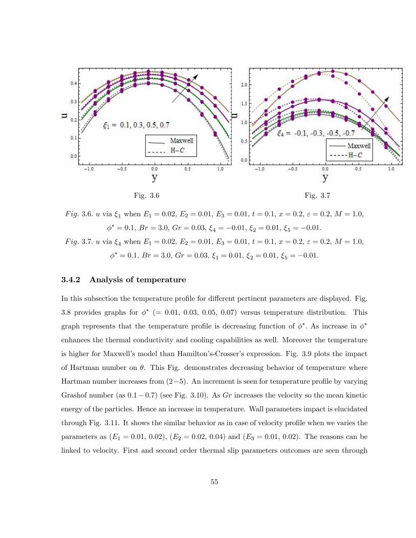
Fig. 3.6 Fig. 3.7
36 via 1 when 1 = 002 2 = 001 3 = 001 = 01 = 02 = 02 = 10
∗ = 01 = 30 = 003 4 = −001 2 = 001 5 = −001 37 via 4 when 1 = 002 2 = 001 3 = 001 = 01 = 02 = 02 = 10
∗ = 01 = 30 = 003 1 = 001 2 = 001 5 = −001
3.4.2 Analysis of temperature
In this subsection the temperature profile for different pertinent parameters are displayed. Fig.
3.8 provides graphs for ∗ (= 001 003 005 007) versus temperature distribution. This
graph represents that the temperature profile is decreasing function of ∗ As increase in ∗
enhances the thermal conductivity and cooling capabilities as well. Moreover the temperature
is higher for Maxwell’s model than Hamilton’s-Crosser’s expression. Fig. 3.9 plots the impact
of Hartman number on . This Fig. demonstrates decreasing behavior of temperature where
Hartman number increases from (2−5). An increment is seen for temperature profile by varyingGrashof number (as 01− 07) (see Fig. 3.10). As increases the velocity so the mean kineticenergy of the particles. Hence an increase in temperature. Wall parameters impact is elucidated
through Fig. 3.11. It shows the similar behavior as in case of velocity profile when we varies the
parameters as (1 = 001 002), (2 = 002 004) and (3 = 001 002). The reasons can be
linked to velocity. First and second order thermal slip parameters outcomes are seen through
55

Figs. 3.12 and 3.13. For an increase of first order thermal slip (2 = 001 003 005 007) the
temperature increases throughout the channel where as for second order thermal slip parameter
(5 = −001 to −007) the temperature increases near the centre. A comparative study revealsthat the temperature remains higher for spherical shaped particles than cylindrical shaped ones.
Fig. 3.8 Fig. 3.9
38 via ∗ when 1 = 002 2 = 001 3 = 001 = 01 = 02 = 02 = 10
= 003 = 30 1 = 001 4 = −001 2 = 001 5 = −001 39 via when 1 = 002 2 = 001 3 = 001 = 01 = 02 = 02 = 003
∗ = 01 = 30 1 = 001 4 = −001 2 = 001 5 = −001
56
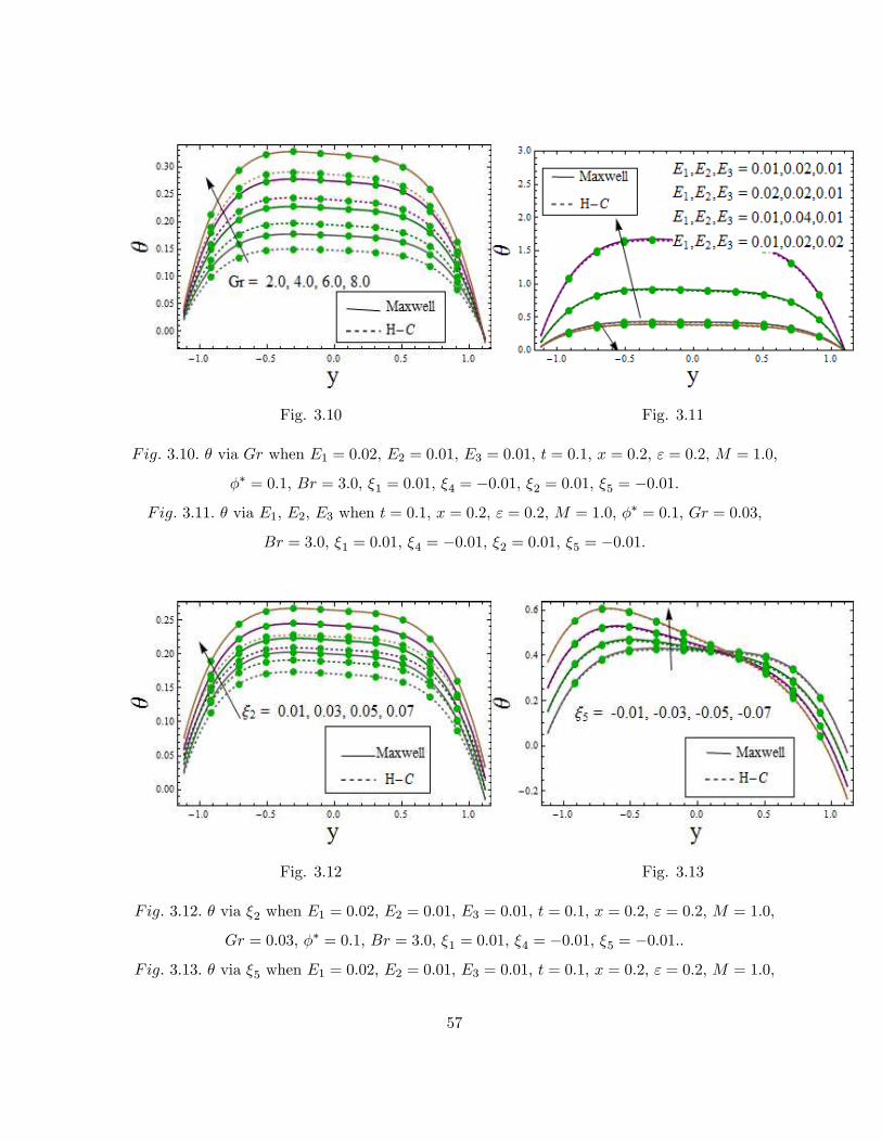
Fig. 3.10 Fig. 3.11
310 via when 1 = 002 2 = 001 3 = 001 = 01 = 02 = 02 = 10
∗ = 01 = 30 1 = 001 4 = −001 2 = 001 5 = −001 311 via 1 2 3 when = 01 = 02 = 02 = 10 ∗ = 01 = 003
= 30 1 = 001 4 = −001 2 = 001 5 = −001
Fig. 3.12 Fig. 3.13
312 via 2 when 1 = 002 2 = 001 3 = 001 = 01 = 02 = 02 = 10
= 003 ∗ = 01 = 30 1 = 001 4 = −001 5 = −001 313 via 5 when 1 = 002 2 = 001 3 = 001 = 01 = 02 = 02 = 10
57
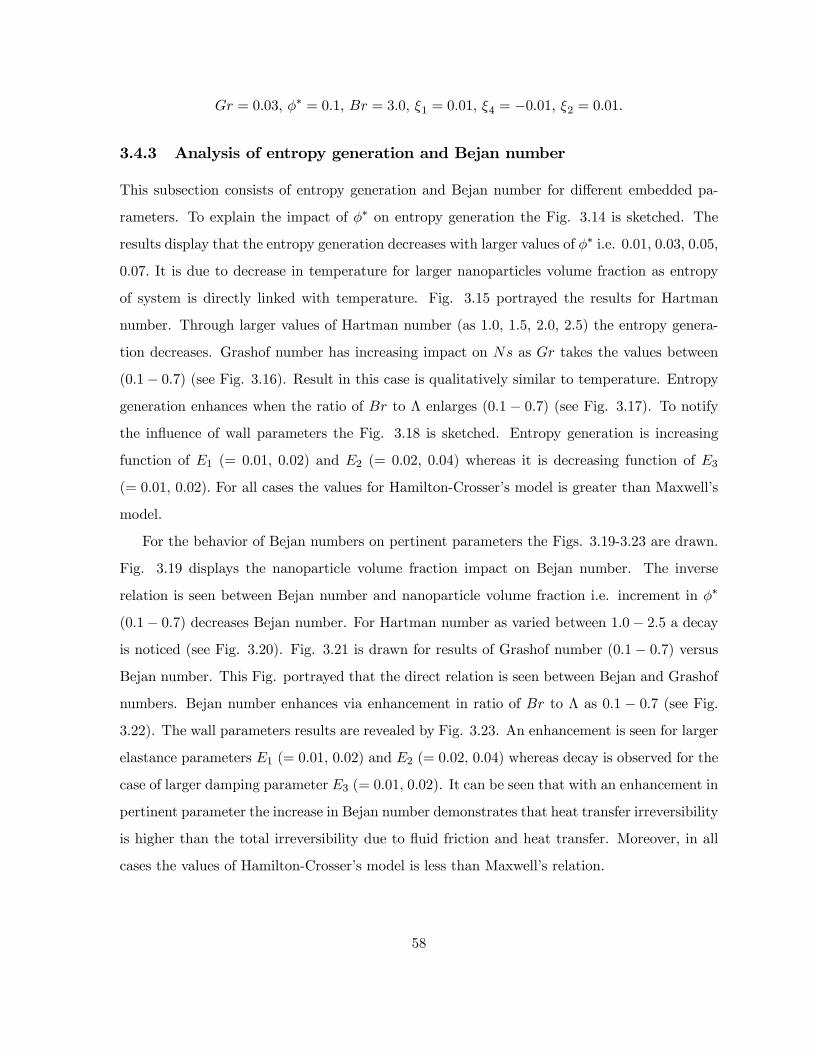
= 003 ∗ = 01 = 30 1 = 001 4 = −001 2 = 001
3.4.3 Analysis of entropy generation and Bejan number
This subsection consists of entropy generation and Bejan number for different embedded pa-
rameters. To explain the impact of ∗ on entropy generation the Fig. 3.14 is sketched. The
results display that the entropy generation decreases with larger values of ∗ i.e. 001 003 005
007 It is due to decrease in temperature for larger nanoparticles volume fraction as entropy
of system is directly linked with temperature. Fig. 3.15 portrayed the results for Hartman
number. Through larger values of Hartman number (as 10 15 20 25) the entropy genera-
tion decreases. Grashof number has increasing impact on as takes the values between
(01− 07) (see Fig. 3.16). Result in this case is qualitatively similar to temperature. Entropygeneration enhances when the ratio of to Λ enlarges (01 − 07) (see Fig. 3.17). To notifythe influence of wall parameters the Fig. 3.18 is sketched. Entropy generation is increasing
function of 1 (= 001 002) and 2 (= 002 004) whereas it is decreasing function of 3
(= 001 002) For all cases the values for Hamilton-Crosser’s model is greater than Maxwell’s
model.
For the behavior of Bejan numbers on pertinent parameters the Figs. 3.19-3.23 are drawn.
Fig. 3.19 displays the nanoparticle volume fraction impact on Bejan number. The inverse
relation is seen between Bejan number and nanoparticle volume fraction i.e. increment in ∗
(01− 07) decreases Bejan number. For Hartman number as varied between 10− 25 a decayis noticed (see Fig. 3.20). Fig. 3.21 is drawn for results of Grashof number (01− 07) versusBejan number. This Fig. portrayed that the direct relation is seen between Bejan and Grashof
numbers. Bejan number enhances via enhancement in ratio of to Λ as 01 − 07 (see Fig.3.22). The wall parameters results are revealed by Fig. 3.23. An enhancement is seen for larger
elastance parameters 1 (= 001 002) and 2 (= 002 004) whereas decay is observed for the
case of larger damping parameter 3 (= 001 002). It can be seen that with an enhancement in
pertinent parameter the increase in Bejan number demonstrates that heat transfer irreversibility
is higher than the total irreversibility due to fluid friction and heat transfer. Moreover, in all
cases the values of Hamilton-Crosser’s model is less than Maxwell’s relation.
58
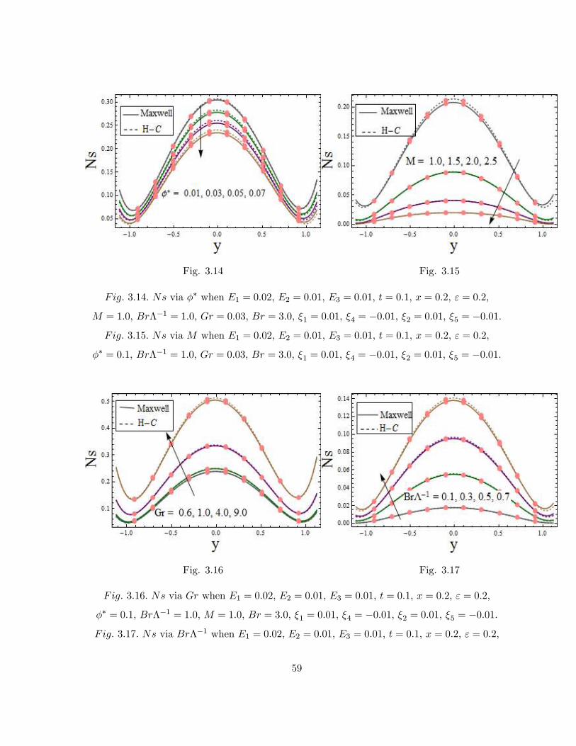
Fig. 3.14 Fig. 3.15
314 via ∗ when 1 = 002 2 = 001 3 = 001 = 01 = 02 = 02
= 10 Λ−1 = 10 = 003 = 30 1 = 001 4 = −001 2 = 001 5 = −001 315 via when 1 = 002 2 = 001 3 = 001 = 01 = 02 = 02
∗ = 01 Λ−1 = 10 = 003 = 30 1 = 001 4 = −001 2 = 001 5 = −001
Fig. 3.16 Fig. 3.17
316 via when 1 = 002 2 = 001 3 = 001 = 01 = 02 = 02
∗ = 01 Λ−1 = 10 = 10 = 30 1 = 001 4 = −001 2 = 001 5 = −001 317 via Λ−1 when 1 = 002 2 = 001 3 = 001 = 01 = 02 = 02
59

∗ = 01 = 10 = 003 = 30 1 = 001 4 = −001 2 = 001 5 = −001
Fig. 3.18 Fig. 3.19
318 via 1 2 3 when = 01 = 02 = 02 ∗ = 01 Λ−1 = 10 = 10
= 003 = 30 1 = 001 4 = −001 2 = 001 5 = −001 319 via ∗ when 1 = 002 2 = 001 3 = 001 = 01 = 02 = 02
= 10 Λ−1 = 10 = 003 = 30 1 = 001 4 = −001 2 = 001 5 = −001
Fig. 3.20 Fig. 3.21
320 via when 1 = 002 2 = 001 3 = 001 = 01 = 02 = 02
∗ = 01 Λ−1 = 10 = 003 = 30 1 = 001 4 = −001 2 = 001 5 = −001
60

321 via when 1 = 002 2 = 001 3 = 001 = 01 = 02 = 02
∗ = 01 Λ−1 = 10 = 10 = 30 1 = 001 4 = −001 2 = 001 5 = −001
Fig. 3.22 Fig. 3.23
322 via Λ−1 when 1 = 002 2 = 001 3 = 001 = 01 = 02 = 02
∗ = 01 = 10 = 003 = 30 1 = 001 4 = −001 2 = 001 5 = −001 323 via 1 2 3 when = 01 = 02 = 02 ∗ = 01 Λ−1 = 10
= 003 = 30 1 = 001 4 = −001 2 = 001 5 = −001
3.4.4 Streamlines
The streamlines are plotted for description of trapping. Fig. 3.24 (a) and (b) displayed the
impact of Hartman number for Maxwell model whereas Fig. 3.24 (c) and (d) portrayed the
influence for Hamilton Crosser model. For both cases the size of trapped bolus increases with
higher values of Hartman number ( = 10 20). Figs. 3.25 and 3.26 (a) -(d) are sketched
for behavior of first and second order slip parameters. These streamlines indicate that trapped
bolus size enhances via increase in first order slip as (001 003) and second order slip parameter
as (−001 −003). Walls parameters impact for Maxwell model can be observed via Fig. 3.27(a)-(d). However Figs. 3.27 (e)-(h) are for Hamilton-Crosser model. Both models show same
behavior for these parameters i.e. trapped bolus size increases for 1 (= 07 09) and 2 (= 04
06) whereas decrease is noticed for 3 (= 02 05)
61

Fig. 3.24 (a) (b)
(c) (d)
324 via for Maxwell model when 1 = 002 2 = 001 3 = 001 = 0 = 02
∗ = 01 = 003 = 30 1 = 001 4 = −001 2 = 001 5 = −001 () = 10 ()
= 20
324 via for Hamilton- Crosser model when 1 = 002 2 = 001 3 = 001 = 0
= 02 ∗ = 01 = 003 = 30 1 = 001 4 = −001 2 = 001 5 = −001 ()
62

= 10 () = 20
Fig. 3.25 (a) (b)
(c) (d)
325 via 1 for Maxwell model when 1 = 002 2 = 001 3 = 001 = 0 = 02
∗ = 01 = 10 = 003 = 30 4 = −001 2 = 001 5 = −001 () 1 = 001 ()1 = 003
325 via 1 for Hamilton- Crosser model when 1 = 002 2 = 001 3 = 001 = 0
= 02 ∗ = 01 = 10 = 003 = 30 4 = −001 2 = 001 5 = −001 ()
63

1 = 001 () 1 = 003
Fig. 3.26 (a) (b)
(c) (d)
326 via 4 for Maxwell model when 1 = 002 2 = 001 3 = 001 = 0 = 02
∗ = 01 = 10 = 003 = 30 1 = 001 2 = 001 5 = −001 () 4 = −001 ()4 = −003
326 via 4 for Hamilton- Crosser model when 1 = 002 2 = 001 3 = 001 = 0
64

= 02 ∗ = 01 = 10 = 003 = 30 1 = 001 2 = 001 5 = −001 ()4 = −001 () 4 = −003
Fig. 3.27 (a) (b)
(c) (d)
65

(e) (f)
(g) (h)
327 via 1 2 3 for Maxwell model when = 0 = 02 ∗ = 01 = 10
= 003 = 30 1 = 001 4 = −001 2 = 001 5 = −001 () 1 = 07 2 = 043 = 02 () 1 = 09 2 = 04 3 = 02 () 1 = 07 2 = 06 3 = 02 () 1 = 07
2 = 04 3 = 05
327 via 1 2 3 for Hamilton- Crosser model when = 0 = 02 ∗ = 01
= 10 = 003 = 30 1 = 001 4 = −001 2 = 001 5 = −001 () 1 = 072 = 04 3 = 02 () 1 = 09 2 = 04 3 = 02 () 1 = 07 2 = 06 3 = 02 ()
66

1 = 07 2 = 04 3 = 05
3.5 Conclusions
The key findings of this chapter are:
• Enhancement in velocity is seen for both first order and second order velocity slip in bothmodels whereas reduction is observed for case of nanoparticle volume fraction.
• The values in Hamilton-Crosser model remain higher than Maxwell’s model especiallynear the centre of channel for the case of velocity profile.
• Grashof and Hartman numbers for velocity have opposite effect.
• Results obtained indicate that temperature in Maxwell’s model exceed than Hamilton-Crosser model.
• Enhancement is observed in entropy generation number for larger Λ−1 and Grashofnumber. Moreover inverse behavior of entropy generation number is obtained for the case
of Hartman number and nanoparticle volume fraction.
• Bolus sizes increases in trapping phenomenon for the case of both first and second ordervelocity slip parameters.
• Bolus size reduces for 3 and it enhances for 1 and 2 in both models.
67

Chapter 4
Modeling and analysis of peristalsis
of hybrid nanofluid with entropy
generation
4.1 Introduction
This chapter intends to explore the peristaltic transport of rotating fluid in a channel. The
channel is considered symmetric with flexible walls and porous medium. In this analysis hybrid
nanofluids consisting of titanium oxides and copper particles. Water is used as the base fluid.
MHD and Hall effects are employed in this problem. Formulation of energy equation is based
on radiation and non uniform heat source or sink. Convective conditions are utilized. Ther-
modynamics second relation is employed for entropy generation. Maxwell-Garnetts model of
thermal conductivity is employed. Numerical analysis is carried out using NDSolve of Mathe-
matica. Graphs are plotted for the axial velocity, secondary velocity, temperature and entropy
generation. Bar graphs are made for the analysis of heat transfer rate at the wall. Streamlines
are displayed for trapping phenomenon. This study declares that enhancement in rotation pa-
rameter caused increase in secondary velocity. Moreover higher values of nanoparticle volume
fraction caused decay in fluid velocity, temperature and entropy. This study further disclosed
that heat transfer rate by higher volume fraction of nanoparticles enhances and more porous
68

structure lead to enhancement in fluid velocity, temperature and entropy.
4.2 Problem modeling
Here we consider the peristalsis of rotating fluid in a symmetric channel (see Fig. 4.1). The
walls of channel have flexible characteristics. Porous medium is saturated by the fluid. MHD
with Hall effects and Joule heating is accounted. Non-uniform heat source and sink parameter
is present. The channel and fluid are in rigid body rotation. The hybrid nanofluid comprising of
2 and nanoparticles with water as base liquid is utilized. The selection of the coordinates
are considered in such a way that x-axis is taken along the flow direction whereas z-axis normal
to it. The walls of channel are taken at temperature 1 and 0 respectively. Thermal radiation
is also present. Rotation is about z-axis with the angular frequency Ω Peristaltic wave of
involuntary contraction and expansion is responsible for the fluid flow. Wave shape is defined
as follows:
= ± ( ) = ±∙+ sin
2
(− )
¸ (4.1)
where represents the width of channel, the wave amplitude, the wavelength and wave
speed.
Fig. 4.1: Schematic Diagram
Related equations satisfy
+
= 0 (4.2)
69
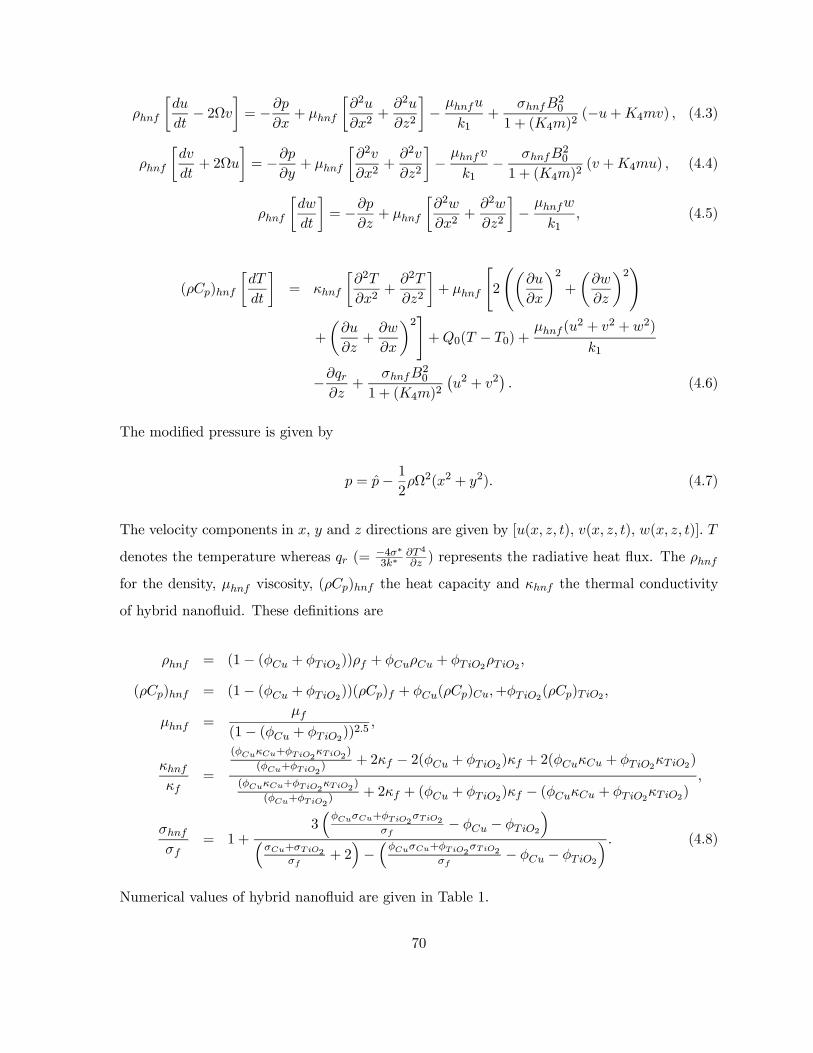
∙
− 2Ω
¸= −
+
∙2
2+
2
2
¸−
1+
20
1 + (4)2(−+4) (4.3)
∙
+ 2Ω
¸= −
+
∙2
2+
2
2
¸−
1−
20
1 + (4)2( +4) (4.4)
∙
¸= −
+
∙2
2+
2
2
¸−
1 (4.5)
()
∙
¸=
∙2
2+
2
2
¸+
"2
õ
¶2+
µ
¶2!
+
µ
+
¶2#+0( − 0) +
(2 + 2 + 2)
1
−
+
20
1 + (4)2
¡2 + 2
¢ (4.6)
The modified pressure is given by
= − 12Ω2(2 + 2) (4.7)
The velocity components in and directions are given by [( ) ( ) ( )]
denotes the temperature whereas (=−4∗3∗
4
) represents the radiative heat flux. The
for the density, viscosity, () the heat capacity and the thermal conductivity
of hybrid nanofluid. These definitions are
= (1− ( + 2)) + + 22
() = (1− ( + 2))() + ()+2()2
=
(1− ( + 2))25
=
(+22)
(+2)
+ 2 − 2( + 2) + 2( + 22)
(+22)
(+2)
+ 2 + ( + 2) − ( + 22)
= 1 +
3³+2
2
− − 2
´³+2
+ 2´−³+2
2
− − 2
´ (4.8)
Numerical values of hybrid nanofluid are given in Table 1.
70

Table 1: Thermophysical parameters of water and nanoparticles [190]
(kg m−3) (j kg−1 K−1) ¡W m−1K−1
¢ (Ω)−1
2 997.1 4179 0.613 0.05
8933 765 401 5.96×10⁷
2 4250 686.2 8.9538 1×10⁻¹²
The boundary conditions for the considered flow are
= 0 at = ± (4.9)
= 0 at = ± (4.10)
∙−∗
3
3+∗
3
2+ ∗1
2
¸ =
∙2
2+
2
2
¸−
1+
20
1 + (4)2(−+4)
−£− 2Ω¤
at = ±(4.11)
=
⎧⎨⎩ −1( − 1)
−2(0 − )
⎫⎬⎭ at = ± (4.12)
in which (i=1, 2) are heat transfer coefficients, ∗ ∗ and ∗1 are the compliant walls
coefficients.
The quantities in dimensionless form are given by
∗ =
∗ =
∗ =
∗ =
∗ =
=
∗ =
∗ =
∗ =
∗1 =
1
2 ∗ =
2
= − 0
1 − 0 =
= −
(4.13)
After using the non-dimensional parameters and utilizing stream function and lubrication ap-
proach we arrive at
= 2
03 +2
3
3− 2
1
+
42
1 + (4)2
µ−
+4
¶ (4.14)
71

= −2 0
3
+2
2
2− 2
1 − 4
2
1 + (4)2( +4) (4.15)
= 0 (4.16)
0 = 12
2+2
µ2
2
¶2+
2
2+
2
1
õ
¶2+ 2
!+
42
1 + (4)2
õ
¶2+ 2
!+ (4.17)
where
1 =
(+22 )
(+2)
+ 2 − 2( + 2) + 2( + 22)
(+22 )
(+2)
+ 2 + ( + 2) − ( + 22)
2 =1
(1− ( + 2))25
3 = (1− ( + 2)) + + 22
4 = 1 +3³+2
2
− − 2
´³+2
+ 2´−³+2
2
− − 2
´ (4.18)
where the non-dimensional parameters are
0=
ReΩ
=
16∗ 303∗
=
r
0 =
0
Pr =()
=
2
() (1 − 0) = Pr =
02
(4.19)
Here 0denotes the Taylor number, the radiation parameter, the Hartman number,
the Hall parameter, Pr the Prandtl number, the Eckert number, the Brinkman number
and the heat source or sink parameter. Note that asterisks have been omitted for brevity.
72

The conditions now become
= 0 = 0 at = ±
+
1
1( − 1) = 0 at =
− 2
1() = 0 at = − (4.20)
∙1
3
3+2
3
2+3
2
¸ = 2
03 +2
3
3− 2
1
+ 42
1+(4)2
³−
+4
´
at = ±(4.21)
in which1 (= 1 ) and2 (= 2 ) are the Biot numbers whereas the wall parameters
1(= −∗33 ) 2(= ∗33 ) and 3(= ∗132 ) are respective elastance and
damping coefficients.
4.2.1 Entropy generation
Entropy generation is given by
000 =
2
õ
¶2+
µ
¶2!+
1
2
16∗ 303∗
µ
¶2+
(2 + 2 +2)
1+Φ
+1
µ
20
1 + (4)2
¡2 + 2
¢¶+
1
(0( − 0)) (4.22)
Expression for viscous dissipation is
Φ =
"2
õ
¶2+
µ
¶2!+
µ
+
¶2# (4.23)
73

In dimensionless form
=000
000
= (1 +)
µ
¶2+
2
Λ
µ2
2
¶2+
2
Λ1
õ
¶2+ 2
!
+4
2
1 + (4)2
Λ
õ
¶2+ 2
!+
Λ (4.24)
000 =
(1 − 0)2
22
Λ =1 − 0
(4.25)
4.3 Analysis
Here we have adopted the NDSolve techniques of Mathematica 9.0 for the solutions. The com-
putation has been carried out by varying the value in the following range: nanoparticle volume
fraction (0.01-0.08), Taylor number (0.1-4.0), Hartman number (0.5-3.5), porosity parameter
(1.0-4.0), Hall parameter (0.1-4.0), radiation parameter (0.1-3.5), Brinkman number (1.0-4.0)
source parameter (0.1-1.0), Biot numbers (4.0-10.0) and wall parameters (0.01-0.3).
4.3.1 Velocity
This subsection has been arranged for velocity. The subsections are arranged here to avoid
complexity.
Axial velocity
This subsection contains information about the results of axial velocity via nanoparticle volume
fraction, Taylor number, Hartman number, porosity parameter, Hall parameter and wall para-
meters. Increasing values of nanoparticle volume fraction enhance the resistance to flow. It is
due to the fact that shear rate increases by enhancing the nanoparticle volume fraction. This
may lead to decrease in axial velocity. Similar behavior is captured here for hybrid nanofluid
through Fig. 4.2. Fig. 4.3 is made for the influence of Taylor number on axial velocity. As
rotation caused the fluid motion in the secondary direction. It leads to decay the velocity in
the axial direction. Hartman number effect can be seen via Fig. 4.4. Higher value of it caused
decrease in the axial velocity as fluid offers more resistance because of Lorentz force. Fig. 4.5
74

portrayed the effect of porosity parameter on axial velocity. As more pores assist the velocity
of fluid. So enhancement is observed. Fig. 4.6 presented the Hall parameter influence on ve-
locity. It leads to enhancement in velocity profile. Moreover as elastance parameters provide
less obstacles to fluid flow so axial velocity enhances for 1 and 2 whereas damping resists
the motion of fluid so velocity decays against 3 (see Fig. 4.7)
Fig. 4.2 Fig. 4.3
42 Axial velocity distribution for and 2 when 1 = 003 2 = 003 3 = 001
0= 01 = 01 = 02 = 02 = 10 = 10 = 10 1 = 4 2 = 6 = 30
1 = 1 = 1
43 Axial velocity distribution for 0when 1 = 003 2 = 003 3 = 001 = 01
= 02 = 02 = 2 = 001 = 10 = 10 = 10 1 = 4 2 = 6 = 30
1 = 1 = 1
75

Fig. 4.4 Fig. 4.5
44 Axial velocity distribution for when 1 = 003 2 = 003 3 = 001 0= 01
= 01 = 02 = 02 = 2 = 001 = 10 = 10 1 = 4 2 = 6 = 30
1 = 1 = 1
45 Axial velocity distribution for 1 when 1 = 003 2 = 003 3 = 001 0= 01
= 01 = 02 = 02 = 2 = 001 = 10 = 10 = 10 1 = 4 2 = 6
= 30 = 1
Fig. 4.6 Fig. 4.7
46 Axial velocity distribution for when 1 = 003 2 = 003 3 = 001 0= 01
76
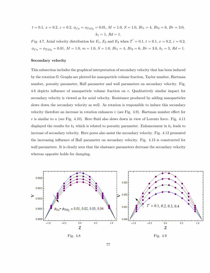
= 01 = 02 = 02 = 2 = 001 = 10 = 10 1 = 4 2 = 6 = 30
1 = 1 = 1
47 Axial velocity distribution for 1 2 and 3 when 0= 01 = 01 = 02 = 02
= 2 = 001 = 10 = 10 = 10 1 = 4 2 = 6 = 30 1 = 3 = 1
Secondary velocity
This subsection includes the graphical interpretation of secondary velocity that has been induced
by the rotation ΩGraphs are plotted for nanoparticle volume fraction, Taylor number, Hartman
number, porosity parameter, Hall parameter and wall parameters on secondary velocity. Fig.
4.8 depicts influence of nanoparticle volume fraction on Qualitatively similar impact for
secondary velocity is viewed as for axial velocity. Resistance produced by adding nanoparticles
slows down the secondary velocity as well. As rotation is responsible to induce this secondary
velocity therefore an increase in rotation enhances (see Fig. 4.9). Hartman number effect for
is similar to (see Fig. 4.10). Here fluid also slows down in view of Lorentz force. Fig. 4.11
displayed the results for 1 which is related to porosity parameter. Enhancement in 1 leads to
increase of secondary velocity. Here pores also assist the secondary velocity. Fig. 4.12 presented
the increasing influence of Hall parameter on secondary velocity. Fig. 4.13 is constructed for
wall parameters. It is clearly seen that the elastance parameters decrease the secondary velocity
whereas opposite holds for damping.
Fig. 4.8 Fig. 4.9
77

48 Secondary velocity distribution for and 2 when 1 = 00002 2 = 00001
3 = 001 0= 01 = 01 = 02 = 02 = 10 = 10 = 10 1 = 4 2 = 6
= 30 1 = 1 = 1
49 Secondary velocity distribution for 0when 1 = 00002 2 = 00001 3 = 001
= 01 = 02 = 02 = 2 = 001 = 10 = 10 = 10 1 = 4 2 = 6
= 30 1 = 1 = 1
Fig. 4.10 Fig. 4.11
410 Secondary velocity distribution for when 1 = 00002 2 = 00001 3 = 001
0= 01 = 01 = 02 = 02 = 2 = 001 = 10 = 10 1 = 4 2 = 6
= 30 1 = 1 = 1
411 Secondary velocity distribution for 1 when 1 = 00002 2 = 00001 3 = 001
0= 01 = 01 = 02 = 02 = 2 = 001 = 10 = 10 = 10 1 = 4
2 = 6 = 30 = 1
78

Fig. 4.12 Fig. 4.13
412 Secondary velocity distribution for when 1 = 00002 2 = 00001 3 = 001
0= 01 = 01 = 02 = 02 = 2 = 001 = 10 = 10 1 = 4 2 = 6
= 30 1 = 1 = 1
413 Secondary velocity distribution for 1 2 and 3 when 0= 01 = 01 = 02
= 02 = 2 = 001 = 10 = 10 = 10 1 = 4 2 = 6 = 30 1 = 1
= 1
4.3.2 Temperature
Temperature containing hybrid nanoparticles are studied in this subsection. Fig. 4.14 is pre-
pared to observe the change in temperature via increasing values of volume fraction. Addition
of nanoparticles in base fluid enhances the heat transfer ability of fluid. It leads to decay the
temperature. Taylor number effect on is checked through Fig. 4.15. 0leads to decrease
the temperature. Fig. 4.16 witnessed the result for Hartman number Temperature en-
hancement is possible here. This is possible in view of Joule heating. Fig. 4.17 reveals the
radiation parameter effect on temperature. Decay is observed clearly. Larger values of poros-
ity parameter lead to enhance the temperature (see Fig. 4.18). Physical reasoning is directly
related to velocity of fluid. Fig. 4.19 shows Brinkman number impact which is responsible for
an enhancement of Brinkman number is directly related to viscous dissipation which results
79

in increase of temperature. Fig. 4.20 depicted the results for Hall parameter on temperature.
Enhancement is observed here. The results can be related with velocity. Heat source parameter
effect on temperature can be viewed via Fig. 4.21. Obviously heat source parameter leads to
enhancement in Figs. 4.22 and 4.23 displayed the results for Biot numbers. In both cases the
temperature profile decays. Fig. 4.24 elucidates the wall parameters influence on Damping
coefficient leads to decrease the temperature whereas opposite is seen for elastance variable.
Fig. 4.14 Fig. 4.15
414 Temperature distribution for and 2 when 1 = 03 2 = 03 3 = 001
0= 10 = 01 = 02 = 02 = 10 = 10 = 05 1 = 8 2 = 10 = 30
1 = 1 = 1
415 Temperature distribution for 0when 1 = 03 2 = 03 3 = 001 = 01
= 02 = 02 = 2 = 001 = 10 = 10 = 05 1 = 8 2 = 10
= 30 1 = 1 = 1
80

Fig. 4.16 Fig. 4.17
416 Temperature distribution for when 1 = 03 2 = 03 3 = 001 0= 10
= 01 = 02 = 02 = 2 = 001 = 10 = 05 1 = 8 2 = 10 = 30
1 = 1 = 1
417 Temperature distribution for when 1 = 03 2 = 03 3 = 001 0= 10
= 01 = 02 = 02 = 2 = 001 = 10 = 10 = 05 1 = 8 2 = 10
= 30 1 = 1
Fig. 4.18 Fig. 4.19
418 Temperature distribution for 1 when 1 = 03 2 = 03 3 = 001 0= 10
81

= 01 = 02 = 02 = 2 = 001 = 10 = 10 = 05 1 = 8 2 = 10
= 30 = 1
419 Temperature distribution for when 1 = 03 2 = 03 3 = 001 0= 10
= 01 = 02 = 02 = 2 = 001 = 10 = 10 = 05 1 = 8 2 = 10
1 = 1 = 1
Fig. 4.20 Fig. 4.21
420 Temperature distribution for when 1 = 03 2 = 03 3 = 001 0= 10
= 01 = 02 = 02 = 2 = 001 = 10 = 05 1 = 8 2 = 10 = 30
1 = 1 = 1
421 Temperature distribution for when 1 = 03 2 = 03 3 = 001 0= 10
= 01 = 02 = 02 = 2 = 001 = 10 = 10 1 = 8 2 = 10 = 30
1 = 1 = 1
82

Fig. 4.22 Fig. 4.23
422 Temperature distribution for 1 when 1 = 03 2 = 03 3 = 001 0= 10
= 01 = 02 = 02 = 2 = 001 = 10 = 10 = 05 2 = 10 = 30
1 = 1 = 1
423 Temperature distribution for 2 when 1 = 03 2 = 03 3 = 001 0= 10
= 01 = 02 = 02 = 2 = 001 = 10 = 10 = 05 1 = 8 = 30
1 = 1 = 1
Fig. 4.24
424 Temperature distribution for 1 2 and 3 when 0= 10 = 01 = 02
83

= 02 = 2 = 001 = 10 = 10 = 05 1 = 8 2 = 10 = 30 1 = 1
= 1
4.3.3 Entropy generation analysis
Figs. 4.25-4.32 are plotted in this subsection for the analysis of entropy of system. Fig. 4.25 is
sketched for the nanoparticle volume fraction onAn increase in nanoparticle volume fraction
reduces the temperature and hence entropy. Similar reasoning is satisfied for the Taylor number
(see Fig. 4.26). Fig. 4.27 provides the results of 1 on entropy. In this case the porosity is
directed linked with temperature. Fig. 4.28 clearly indicates that viscous dissipation leads to
an increase in and Fig. 4.29 states that Hartman number increases the entropy due to
Joule heating. Heat source parameter leads to increase in entropy (see Fig. 4.30). Fig. 4.31
presents the Hall parameter influence. Enhancement is noticed in this case. Fig. 4.32 displays
that with ( = 1 2) the entropy enlarges whereas 3 leads to decrease the entropy.
Fig. 4.25 Fig. 4.26
425 Entropy generation for and 2 when 1 = 002 2 = 001 3 = 001
0= 01 = 01 = 02 = 02 = 10 = 10 = 05 1 = 8 2 = 10 = 30
1 = 1 = 1 Λ = 05
426 Entropy generation for 0when 1 = 002 2 = 001 3 = 001 = 01 = 02
= 02 = 2 = 001 = 10 = 10 = 05 1 = 8 2 = 10 = 30 1 = 1
84
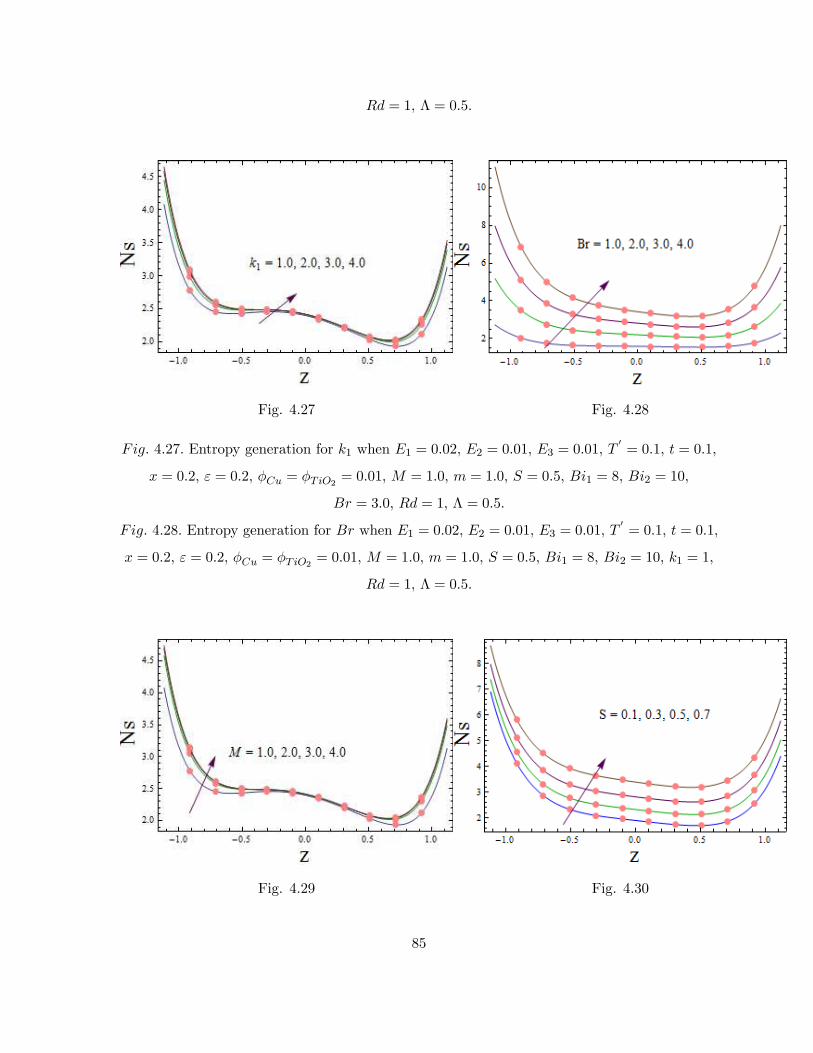
= 1 Λ = 05
Fig. 4.27 Fig. 4.28
427 Entropy generation for 1 when 1 = 002 2 = 001 3 = 001 0= 01 = 01
= 02 = 02 = 2 = 001 = 10 = 10 = 05 1 = 8 2 = 10
= 30 = 1 Λ = 05
428 Entropy generation for when 1 = 002 2 = 001 3 = 001 0= 01 = 01
= 02 = 02 = 2 = 001 = 10 = 10 = 05 1 = 8 2 = 10 1 = 1
= 1 Λ = 05
Fig. 4.29 Fig. 4.30
85
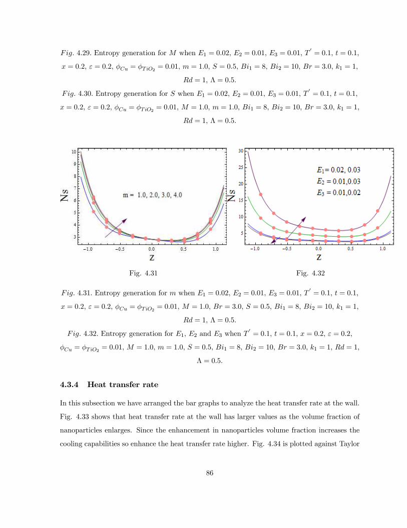
429 Entropy generation for when 1 = 002 2 = 001 3 = 001 0= 01 = 01
= 02 = 02 = 2 = 001 = 10 = 05 1 = 8 2 = 10 = 30 1 = 1
= 1 Λ = 05
430 Entropy generation for when 1 = 002 2 = 001 3 = 001 0= 01 = 01
= 02 = 02 = 2 = 001 = 10 = 10 1 = 8 2 = 10 = 30 1 = 1
= 1 Λ = 05
Fig. 4.31 Fig. 4.32
431 Entropy generation for when 1 = 002 2 = 001 3 = 001 0= 01 = 01
= 02 = 02 = 2 = 001 = 10 = 30 = 05 1 = 8 2 = 10 1 = 1
= 1 Λ = 05
432 Entropy generation for 1 2 and 3 when 0= 01 = 01 = 02 = 02
= 2 = 001 = 10 = 10 = 05 1 = 8 2 = 10 = 30 1 = 1 = 1
Λ = 05
4.3.4 Heat transfer rate
In this subsection we have arranged the bar graphs to analyze the heat transfer rate at the wall.
Fig. 4.33 shows that heat transfer rate at the wall has larger values as the volume fraction of
nanoparticles enlarges. Since the enhancement in nanoparticles volume fraction increases the
cooling capabilities so enhance the heat transfer rate higher. Fig. 4.34 is plotted against Taylor
86

number effect. Rotation leads to decrease the heat transfer rate. Hartman number increased
the heat transfer rate at the wall (see Fig. 4.35). Fig. 4.36 portrayed the effect of porosity
parameter on heat transfer rate. An increase in pores enhances the temperature. It means
that there is less heat transfer rate at the wall. Fig. 4.37 demonstrated increasing value of
heat transfer rate at the wall with higher values of Hall parameter. Fig. 4.38 depicted the heat
transfer rate for Brinkman number. Heat transfer rate at wall increases for higher Brinkman
number. Fig. 4.39 is constructed to see the influence of on heat transfer rate. Heat transfer
rate decreases with higher radiation parameter.
Fig. 4.33
433 Heat transfer rate at the wall (−10()) for ∗(= + 2) when 1 = 003
2 = 003 3 = 001 0= 20 = 01 = 0 = 02 = 20 = 20 = 10 1 = 8
2 = 10 = 30 1 = 3 = 05
87

Fig. 4.34
434 Heat transfer rate at the wall (−10()) for
0when 1 = 003 2 = 003
3 = 001 = 01 = 0 = 02 = 2 = 001 = 20 = 20 = 10 1 = 8
2 = 10 = 30 1 = 3 = 05
Fig. 4.35
88

435 Heat transfer rate at the wall (−10()) for when 1 = 003 2 = 003
3 = 001 0= 20 = 01 = 0 = 02 = 2 = 001 = 01 = 10 1 = 8
2 = 10 = 30 1 = 3 = 05
Fig. 4.36
436 Heat transfer rate at the wall (−10()) for 1 when 1 = 003 2 = 003
3 = 001 0= 20 = 01 = 0 = 02 = 2 = 001 = 20 = 20 = 10
1 = 8 2 = 10 = 30 = 05
89

Fig. 4.37
437 Heat transfer rate at the wall (−10()) for when 1 = 003 2 = 003
3 = 001 0= 20 = 01 = 0 = 02 = 2 = 001 = 20 = 10 1 = 8
2 = 10 = 30 1 = 3 = 05
Fig. 4.38
90

438 Heat transfer rate at the wall (−10()) for when 1 = 003 2 = 003
3 = 001 0= 20 = 01 = 0 = 02 = 2 = 001 = 20 = 20 = 10
1 = 8 2 = 10 1 = 3 = 05
Fig. 4.39
439 Heat transfer rate at the wall (−10()) for when 1 = 003 2 = 003
3 = 001 0= 20 = 01 = 0 = 02 = 2 = 001 = 20 = 20 = 10
1 = 8 2 = 10 = 30 1 = 3
4.3.5 Streamlines
Trapping phenomenon has been analyzed in this subsection. Streamlines has been plotted for
this purpose. Fig. 4.40 (a) and (b) describe the impact of volume fraction for hybrid nanofluid.
In is seen that the size of trapped bolus increases as the volume fraction of nanoparticles
enhances. Fig. 4.41 (a) and (b) show the bolus results for increasing values of Taylor number
for hybrid nanofluid. In this case bolus sizes decrease for increasing values of Taylor number.
Porosity parameter effect on streamlines can be seen via Fig. 4.42 (a) and (b) for hybrid
nanofluid. Bolus sizes show a decrease for increasing values of 1 Figs. 4.43, 4.44 (a) and (b)
represent the impact of Hartman number and Hall parameter on bolus size. Decrease is noticed
in both cases.
91

Fig. 4.40 (a) (b)
440 via ∗ for hybrid nanofluid when 1 = 0003 2 = 0003 3 = 001 0= 001
= 0 = 02 = 10 = 10 = 10 1 = 4 2 = 6 = 30 1 = 1 = 1 ()
= 2 = 005 () = 2 = 009
Fig. 4.41 (a) (b)
92

441 via 0for hybrid nanofluid when 1 = 0003 2 = 0003 3 = 001 = 0
= 02 = 10 = 10 = 10 = 2 = 001 1 = 4 2 = 6 = 30 1 = 1
= 1 () 0= 01 ()
0= 02
Fig. 4.42 (a) (b)
442 via 1 for hybrid nanofluid when 1 = 0003 2 = 0003 3 = 001 0= 01
= 0 = 02 = 10 = 10 = 10 = 2 = 001 1 = 4 2 = 6 = 30
93

= 1 () 1 = 1 () 1 = 2
Fig. 4.43 (a) (b)
443 via for hybrid nanofluid when 1 = 0003 2 = 0003 3 = 001 0= 01
= 0 = 02 = 10 = 10 = 2 = 001 1 = 4 2 = 6 = 30 1 = 1
= 1 () = 1 () = 2
Fig. 4.44 (a) (b)
94

444 via for hybrid nanofluid when 1 = 0003 2 = 0003 3 = 001 0= 01
= 0 = 02 = 10 = 10 = 2 = 001 1 = 4 2 = 6 = 30 1 = 1
= 1 () = 1 () = 2
4.4 Conclusions
In this study we scrutinized the hybrid nanofluid in a rotating frame. MHD and Hall effects are
incorporated in the momentum equation. Energy equation includes non-uniform heat source
or sink parameter, radiation and Joule heating. Porous medium is considered in this problem.
Main results of this analysis are concluded as follows.
• Non-Uniform heat source parameter leads to increase in temperature and entropy.
• Hall parameter and Hartman number effects on temperature and entropy are qualitativelysimilar.
• Nanoparticle volume fraction enhancement caused decay in temperature, axial and sec-ondary velocities and entropy.
• Porosity parameters gives rise to axial and secondary velocities, temperature and entropy.
• Enhancement in the rotation caused increase in the secondary velocity whereas oppositebehavior has been observed for axial velocity, temperature and entropy generation.
• Heat transfer rate enhances when we increase the nano particle volume fraction.
• Size of bolus increases for larger volume fraction of nanoparticles whereas it reduces forTaylor and porosity parameters.
95
Chapter 5
Entropy generation in peristaltic
flow of Williamson nanofluid
5.1 Introduction
In this chapter the influences of an inclined magnetic field and Joule heating on peristalsis of
Williamson nanofluid in a complaint walls channel are examined. Analysis is presented when
no-slip conditions for velocity, temperature and concentration are no longer hold. Entropy gen-
eration is discussed. Formulated problem is numerically solved for large wavelength and small
Reynolds number. Main emphasis is given to the outcomes of velocity, temperature, concen-
tration, heat transfer coefficient and entropy generation. The results are discussed graphically.
5.2 Formulation
We examine flow of an electrically conducting Williamson nanofluid in a symmetric channel of
width 2. The channel walls at = ± are compliant in nature. Here = corresponds to
the upper wall whereas the lower wall is taken at = − (see Fig. 5.1). Salient features ofBrownian movement and thermophoresis are accounted. Here -axis is taken along the channel
whereas -axis being normal to . Temperature and concentration of the upper and lower walls
are maintained 1 0 and 1, 0 respectively. The sinusoidal waves traveling along the channel
96

walls are responsible for mechanism of peristalsis. Mathematical shape of such waves [172]:
= ± ( ) = ±∙+ sin
2
(− )
¸ (5.1)
Here is the amplitude of wave, the wavelength, the speed of wave and the time.
Fig. 5.1: Schematic diagram
An inclined magnetic field with inclination is taken. Induced magnetic field for low magnetic
Reynolds number is not accounted. Electric field is absent. Then [172]:
B = [0 sin0 cos 0] (5.2)
where 0 represents magnetic field strength. Lorentz force (F = J×B) now yields [82]:
J×B = £−20 cos( cos− sin) 20 sin( cos− sin) 0¤ (5.3)
Here J(=(V×B)) and V(= [ 0]) are used to signify the electrical conductivity, currentdensity and velocity of the fluid. The expressions which can govern the flow are [172]:
+
= 0 (5.4)
+
+
= − 1
+1
+1
− 1
20 cos( cos− sin) (5.5)
97

+
+
= − 1
+1
+1
+1
20 sin( cos− sin) (5.6)
where depicts the pressure, the component of extra stress tensor and the fluid density.
Expressions of temperature and concentration satisfy [172]:
+
+
= ∗
∙2
2+
2
2
¸+
1
()
∙
+
µ
+
¶+
¸+
"
µ
+
¶+
õ
¶2+
µ
¶2!#+
1
()20( cos− sin)2 (5.7)
+
+
=
µ2
2+
2
2
¶+
µ2
2+
2
2
¶ (5.8)
Here ∗ denotes the thermal diffusivity and the specific heat. Moreover and
define the respective Brownian motion coefficient, thermophoretic diffusion coefficient and
mean temperature of nanofluid. (= () () ) is the ratio of specific heat capacity for
nanomaterial and fluid. Symbols and are used for temperature and concentration of fluid.
For Williamson liquid, the extra stress tensor S satisfies [82, 84]:
S = [∞ + (0 + ∞)(1− Γ)−1]A1 (5.9)
where 0 and ∞ correspond to zero shear rate and infinite shear rate viscosities and Γ the
time constant. Here and A1 are
=
r1
2Π (5.10)
A1 = gradV+ (gradV) (5.11)
Π = (A21) (5.12)
Assuming that ∞ = 0 and Γ 1 then expression of stress tensor for Williamson fluid becomes
S = 0[(1 + Γ)]A1 (5.13)
For Γ = 0 the above expression reduces to incompressible viscous fluid. From Eq. (5.13) we
98

have
= 20(1 + Γ)
(5.14)
= 0(1 + Γ)
µ
+
¶ (5.15)
= 20(1 + Γ)
(5.16)
=
s2
µ
¶2+ 2
µ
¶2+
µ
+
¶2 (5.17)
The boundary conditions for problem are :
± 1 = 0 at = ± (5.18)
∙−∗
3
3+∗
3
2+ ∗1
2
¸ =
+
−
∙
+
+
¸−20 cos( cos− sin) at = ±(5.19)
± 2
=
⎧⎨⎩ 1
0
⎫⎬⎭ at = ± (5.20)
± 3
=
⎧⎨⎩ 1
0
⎫⎬⎭ at = ± (5.21)
In above equations ∗, ∗, and ∗1 represent the elastic tension, mass per unit area and the
coefficient of viscous damping respectively. Extra stress tensor components are given by ,
and whereas 1 2 and 3 denote slip parameters for velocity, temperature and concentration
respectively.
We set the dimensionless quantities as
∗ =
∗ =
∗ =
∗ =
∗ =
∗ =
∗ =
0 ∗ =
∗ =
2
0 = Γ
=
− 0
1 − 0
= − 0
1 − 0 =
= −
(5.22)
99
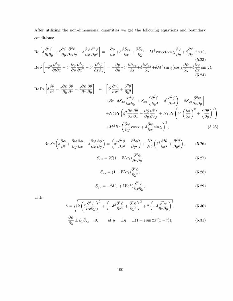
After utilizing the non-dimensional quantities we get the following equations and boundary
conditions:
Re
∙2
+
2
−
2
2
¸= −
+
+
−2 cos(cos
+
sin)
(5.23)
Re
∙−2
2
− 2
2
2− 2
2
¸= −
+2
+
+2 sin(cos
+
sin)
(5.24)
RePr
∙
+
−
¸=
∙22
2+
2
2
¸+
∙
2
+
µ2
2− 2
2
2
¶−
2
¸+Pr
µ2
+
¶+Pr
Ã2µ
¶2+
µ
¶2!
+2
µ
cos+
sin
¶2 (5.25)
Re
µ
+
−
¶=
µ22
2+
2
2
¶+
µ22
2+
2
2
¶ (5.26)
= 2(1 +)2
(5.27)
= (1 +)2
2 (5.28)
= −2(1 +)2
(5.29)
with
=
s2
µ2
¶2+
µ−2
2
2+
2
2
¶2+ 2
µ− 2
¶2 (5.30)
± 1 = 0, at = ± = ±(1 + sin 2 (− )) (5.31)
100

∙1
3
3+2
3
2+3
2
¸ = −Re
∙2
+
2
−
2
2
¸+
+−2 cos
(cos+
sin) at = ±
(5.32)
± 2
=
⎧⎨⎩ 1
0
⎫⎬⎭ at = ± (5.33)
± 3
=
⎧⎨⎩ 1
0
⎫⎬⎭ at = ± (5.34)
The quantities involved above include the amplitude ratio (= ), (= ) wave number,
Re(= 0) Reynolds number, =p00 Hartman number and Williamson fluid
parameter known as Weissenberg number. The Brownian motion parameter, thermophoresis
parameter, Schmidt number, Prandtl number and Brinkman number are (= (1 −0)0) (= (1−0)0) (= 0) Pr(= 0 () ), and(= 20(1−0)) respectively. The dimensionless parameters representing the compliant nature of walls are
1(= −∗330) 2(= ∗330) and 3(= ∗1320) Furthermore the slip parame-
ters for velocity, temperature and concentration are ∗1 = 10 ∗2 = 3 and ∗3 = 3
The systems subject to large wavelength and low Reynolds number are reduced to the
following set of equation whereas the continuity equation is satisfied identically.
=
−2 cos2
(5.35)
= 0 (5.36)
2
2+
2
2+Pr
+Pr
µ
¶2+2
µ
cos
¶2= 0 (5.37)
2
2+
2
2= 0 (5.38)
= 0 = (5.39)
= (1 +)2
2 (5.40)
101

=2
2 (5.41)
± 1 = 0, at = ± = ±(1 + sin 2 (− )) (5.42)
∙1
3
3+2
3
2+3
2
¸ =
−2 cos2
at = ± (5.43)
± 2
=
⎧⎨⎩ 1
0
⎫⎬⎭ at = ± (5.44)
± 3
=
⎧⎨⎩ 1
0
⎫⎬⎭ at = ± (5.45)
From Eqs. (5. 35) and (5.36) we get
∙
−2 cos2
¸= 0 (5.46)
Now we numerically solve the Eqs. (5.37), (5.38) and (5.46) by utilizing the boundary conditions
mentioned in Eqs. (5.42-5.45). NDSolve of Mathematica is utilized for this purpose. The results
are analyzed numerically.
5.2.1 Determination of Entropy generation
Viscous dissipation expression is
Φ =
+
+
µ
+
¶ (5.47)
Dimensional volumetric entropy generation is
000 =
2
õ
¶2+
µ
¶2!| z
+20( cos− sin)2
| z
+Φ
|z
+
õ
¶2+
µ
¶2!+
µ
+
¶| z
(5.48)
102

In dimensionless form one has
=000
000
=
µ
¶2+
2
Λ
µ
cos
¶2+
Λ
µ2
2
¶+
Λ
µ
¶µ
¶+
Λ2
µ
¶2 (5.49)
with
000 =
(1 − 0)2
22
Λ =1 − 0
=
(1 − 0)
=
(1 − 0)
(5.50)
5.3 Analysis
Here the velocity, temperature, concentration, heat transfer coefficient and entropy are exam-
ined via graphs for influence of different parameters. Problem is solved by using NDSolve of
Mathematica. For detail analysis of the results we further divide this section into subsections.
5.3.1 Velocity
This subsection intends to analyze the velocity. Fig. 5.2 (a) has been plotted for Hartman
number () effect. Here decreasing behavior of axial velocity by larger Hartman number is
notified. Such behavior of velocity under the influence of Hartman number is because of resistive
characteristic of Lorentz force. Fig. 5.2 (b) elucidated the influence of slip parameter on velocity.
We have noticed that increasing behavior is seen for velocity against slip parameter. It is due
to less resistance offered by fluid to flow. Fig. 5.2 (c) has been drawn to see the behavior
of wall parameters. Enhancement in elastance parameters 1 and 2 give rise to velocity. It
is because of decrease in resistance by increasing wall elastance parameters. An enhancement
in wall damping coefficient 3 decreases velocity of fluid. Behavior of inclination of magnetic
field on velocity is observed through Fig. 5.2 (d). Increasing behavior has been noticed for
velocity by larger . Effect of Weissenberg number on axial velocity is analyzed in Fig. 5.2 (e).
Weissenberg number for velocity has mixed behavior.
103

Fig. 5.2 (a) Fig. 5.2 (b)
Fig. 5.2 (c) Fig. 5.2 (d)
104

Fig. 5.2 (e)
52 Graphs for when 1 = 002 2 = 001 3 = 001 = 01 = 02 = 02
= 001 1 = 01 2 = 01 3 = 01 = 01 = 01 = 15 = 20 = 10
= 4(a) impact on (b) 1 impact on (c) 1 2 3 impact on (d) impact on
(e) impact on
5.3.2 Temperature
This subsection examined temperature for slip parameter (2), Hartman number () Brownian
motion () thermophoresis parameter () and magnetic field inclination parameter () on
the temperature distribution. Fig. 5.3 (a) characterized temperature for Hartman number.
An enhancement in temperature is observed at center of channel for larger Hartman number.
An increase in temperature is caused by Joule heating phenomenon. Fig. 5.3 (b) has been
prepared just to view the effect of thermal slip parameter on temperature. Enhancement is
seen in temperature by larger slip parameter. The reason can be directly linked with velocity.
Influences of Brownian motion and thermophoresis parameters have been studied through Figs.
5.3 (c) and (d). Temperature is an increasing function of both parameters. As increase in
random motion of particles enhances the mean kinetic energy of the particles and consequently
the temperature. Impact of magnetic field inclination angle on temperature has been observed
via Fig. 5.3 (e). Temperature is enhanced by Obviously magnetic field perpendicular to flow
105

is more effective and it caused more resistance to fluid, here increases the temperature.
Fig. 5.3 (a) Fig. 5.3 (b)
Fig. 5.3 (c) Fig. 5.3 (d)
106

Fig. 5.3 (e)
53 Graphs for when 1 = 002 2 = 001 3 = 001 = 01 = 02 = 02
= 001 1 = 01 2 = 01 3 = 01 = 01 = 01 = 15 = 10 = 20
= 4 (a) impact on (b) 2 impact on (c) impact on (d) impact on (e)
impact on
5.3.3 Concentration
Here concentration is examined with respect to various influential parameters. Fig. 5.4 (a)
displayed concentration for Hartman number. Clearly concentration is an increasing function
of Hartman number. Increase in concentration slip parameter decreases concentration (see Fig.
5.4 (b)). Figs. 5.4 (c) and (d) elucidated effects of Brownian motion and thermophoresis on
concentration. Concentration has opposite behavior for these both parameters. An inverse
relation of these parameters has been observed in the concentration expression.
107

Fig. 5.4 (a) Fig. 5.4 (b)
Fig. 5.4 (c) Fig. 5.4 (d)
54 Graphs for when 1 = 002 2 = 001 3 = 001 = 01 = 02 = 02
= 001 = 01 1 = 01 2 = 01 3 = 01 = 01 = 01 = 15 = 20
= 10 = 4 (a) impact on (b) 3 impact on (c) impact on (d) impact
on
108

5.3.4 Heat transfer coefficient
This subsection has been organized for the description of outcomes of various parameters on
heat transfer coefficient () Impact of Hartman number on is shown in Fig. 5.5 (a). There
is a decrease in for larger . Further an increase in leads to an enhancement of (see
Fig. 5.5 (b)). Furthermore through Figs. 5.5 (c) and (d) the heat transfer coefficient via change
in and has been analyzed. Opposite behavior of heat transfer coefficient through these
parameters is observed. These Figs. witness for an oscillatory behavior.
Fig. 5.5 (a) Fig. 5.5 (b)
Fig. 5.5 (c) Fig. 5.5 (d)
109

55 Graphs for when 1 = 002 2 = 001 3 = 001 = 01 = 02 = 001
1 = 01 2 = 01 3 = 01 = 10 = 10 = 15 = 20 = 10 = 4 (a)
impact on (b) impact on (c) impact on (d) impact on
5.3.5 Entropy generation
This subsection has been prepared to analyze the entropy generation. Thus Figs. 5.6 (a-c) have
been plotted for this purpose. Fig. 5.6 (a) described the influence of Hartman number ()
on It is worth mentioning that is an increasing function of It is in view of Joule
heating aspect. Brownian motion () and thermophoresis impacts have been seen via Figs.
5.6 (b) and (c). Increasing results are noticed for both variables. These results can be verified
in view of directly linked with temperature.
Fig. 5.6 (a) Fig. 5.6 (b)
110

Fig. 5.6 (c)
56 Graphs for when 1 = 002 2 = 001 3 = 001 = 01 = 02 = 02
= 001 1 = 01 2 = 01 3 = 01 = 01 = 01 = 20 = 05 = 05
Λ = 05 = 10 = 15 = 4 (a) impact on (b) impact on (c)
impact on
5.3.6 Validation of problem
Fig. 5.7: Validation of the problem
111

57 via change in and when 1 = 001 2 = 002 3 = 001 = 01 = 02
= 02 = 00 1 = 01 2 = 01 3 = 01 = 10 = 10 = 00 = 00
The purpose of Fig. 5.7 is to validate our results. Here we have chosen a study by Mustafa
et al. [170]. The authors here have studied the nanofluid flow through Buongiorno model. They
have utilized the homotopy analysis method to solve their proposed problem. In our problem
if we exclude the inclined magnetic field and replace the Williamson fluid by viscous fluid we
obtained the results of paper [170].
5.4 Conclusions
Major findings here include the following.
• Velocity is decreasing function of Hartman number and wall damping coefficient (3)whereas it is increasing function of 1 2 and velocity slip parameter.
• and has same behavior on temperature.
• Temperature has same behavior for larger thermal slip parameter and Hartman number().
• Concentration has opposite behavior for concentration slip parameter when comparedwith Hartman number ().
• Heat transfer coefficient for inclination angle for magnetic field has opposite response tothat of Hartman number ().
• and have opposite behavior on heat transfer coefficient.
112
Chapter 6
Effects of radial magnetic field and
entropy on peristalsis of Williamson
fluid in curved channel
6.1 Introduction
This chapter aims to analyze the peristaltic activity of Williamson fluid in curved configuration.
Flow formulation is made by employing radial magnetic field and Soret and Dufour effects.
Slip conditions for velocity, temperature and concentration are applied. Entropy analysis is
also carried out. Modeling is given using lubrication approach. Stream function, velocity,
temperature and concentration solutions have been derived. Effects of different parameters
are analyzed on flow quantities of interest. Moreover streamlines are examined for different
embedded parameters. Result reveals that Lorentz force tends to slow down the fluid velocity.
The slip parameters for velocity and temperature lead to enhancement in corresponding profile
whereas opposite behavior is noticed for concentration. Soret and Dufour effect lead to increase
the temperature as well as entropy of the system. Compliant nature walls increase the fluid
velocity for elastance parameters where as damping nature reduces the fluid velocity.
113

6.2 Modeling
Consider a curved configuration having channel width 2, which is coiled in a circle with centre
at and has radius ∗(see Fig. 6.1). A incompressible electrically conducting Williamson fluid
in channel is taken. Walls of the channel are considered flexible. In radial direction a magnetic
field is applied whose strength is taken . Coordinate system has been taken such as that
both -axis and -axis lie normal to each other. ( ) and ( ) are the respective axial
and radial velocity components. The walls shape satisfies the following expression [50]
= ± ( ) = ±∙+ sin
2
(− )
¸ (6.1)
in which , and elucidate the respective amplitude, wavelength and speed of the wave and
denotes the time.
Fig. 6.1: Sketch of the geometry
The applied magnetic field can be expressed as follows [84]:
B =
∙∗0 +∗
0 0
¸ (6.2)
114
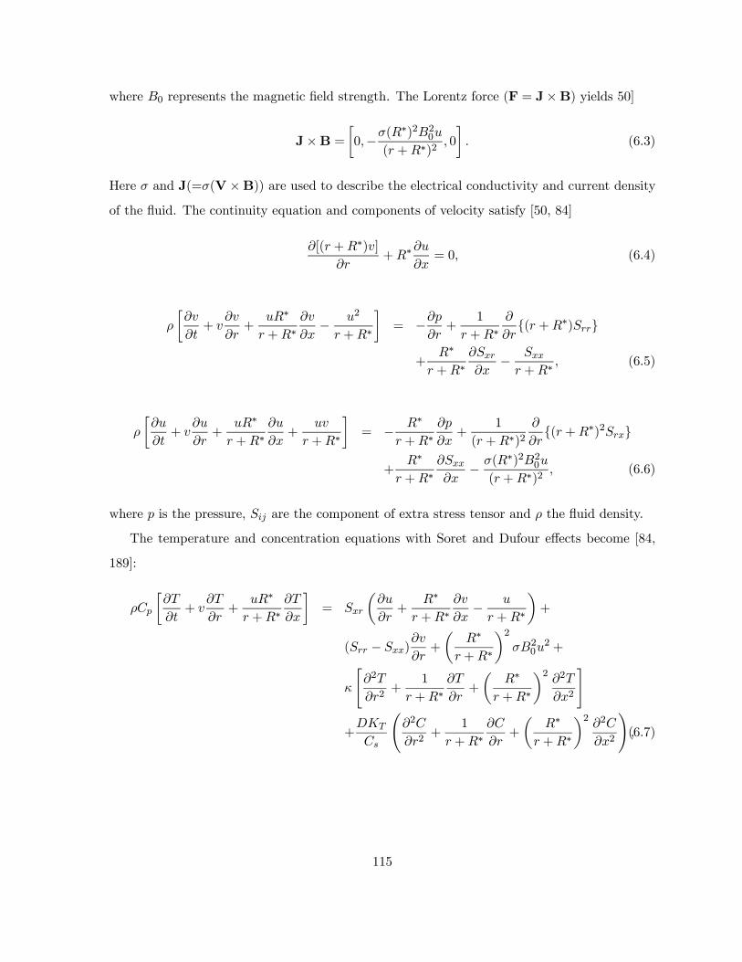
where 0 represents the magnetic field strength. The Lorentz force (F = J×B) yields 50]
J×B =∙0−(
∗)220( +∗)2
0
¸ (6.3)
Here and J(=(V×B)) are used to describe the electrical conductivity and current densityof the fluid. The continuity equation and components of velocity satisfy [50, 84]
[( +∗)]
+∗
= 0 (6.4)
∙
+
+
∗
+∗
− 2
+∗
¸= −
+
1
+∗
( +∗)
+∗
+∗
−
+∗ (6.5)
∙
+
+
∗
+∗
+
+∗
¸= − ∗
+∗
+
1
( +∗)2
( +∗)2
+∗
+∗
− (∗)220( +∗)2
(6.6)
where is the pressure, are the component of extra stress tensor and the fluid density.
The temperature and concentration equations with Soret and Dufour effects become [84,
189]:
∙
+
+
∗
+∗
¸=
µ
+
∗
+∗
−
+∗
¶+
( − )
+
µ∗
+∗
¶220
2 +
"2
2+
1
+∗
+
µ∗
+∗
¶22
2
#
+
Ã2
2+
1
+∗
+
µ∗
+∗
¶22
2
!(6.7)
115
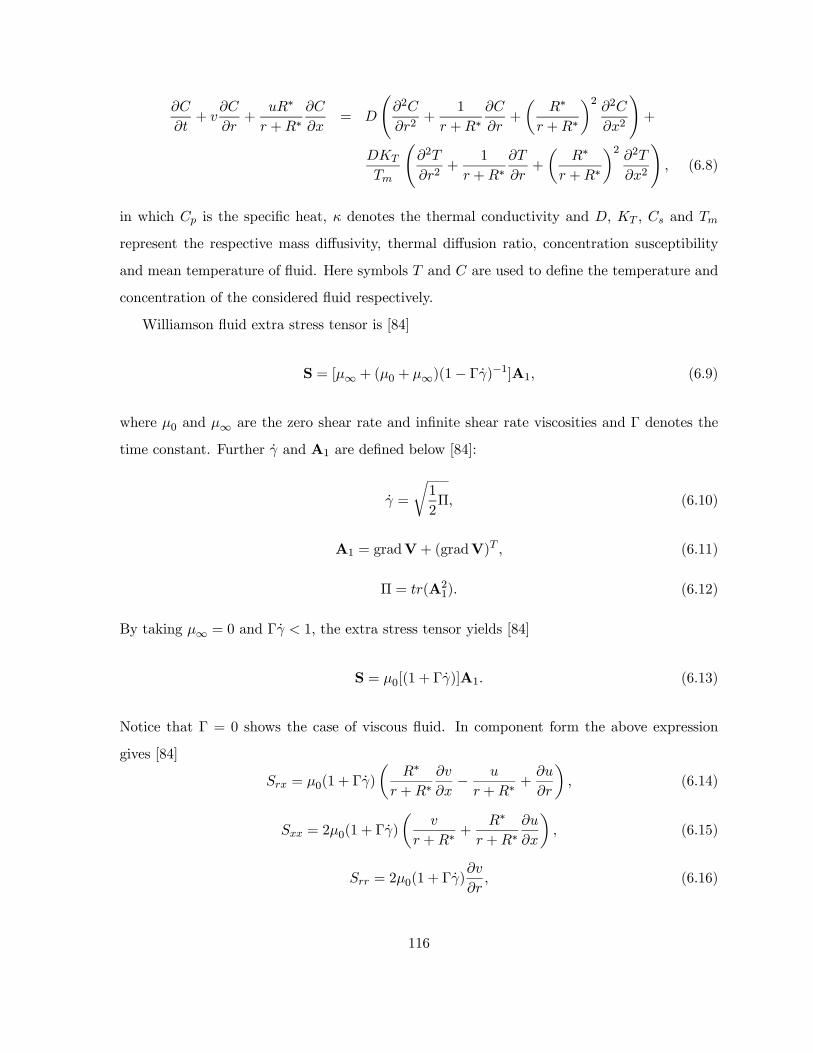
+
+
∗
+∗
=
Ã2
2+
1
+∗
+
µ∗
+∗
¶22
2
!+
Ã2
2+
1
+∗
+
µ∗
+∗
¶22
2
! (6.8)
in which is the specific heat, denotes the thermal conductivity and and
represent the respective mass diffusivity, thermal diffusion ratio, concentration susceptibility
and mean temperature of fluid. Here symbols and are used to define the temperature and
concentration of the considered fluid respectively.
Williamson fluid extra stress tensor is [84]
S = [∞ + (0 + ∞)(1− Γ)−1]A1 (6.9)
where 0 and ∞ are the zero shear rate and infinite shear rate viscosities and Γ denotes the
time constant. Further and A1 are defined below [84]:
=
r1
2Π (6.10)
A1 = gradV+ (gradV) (6.11)
Π = (A21) (6.12)
By taking ∞ = 0 and Γ 1 the extra stress tensor yields [84]
S = 0[(1 + Γ)]A1 (6.13)
Notice that Γ = 0 shows the case of viscous fluid. In component form the above expression
gives [84]
= 0(1 + Γ)
µ∗
+∗
−
+∗+
¶ (6.14)
= 20(1 + Γ)
µ
+∗+
∗
+∗
¶ (6.15)
= 20(1 + Γ)
(6.16)
116

=
s2
µ
¶2+ 2
µ
+∗+
∗
+∗
¶2+
µ∗
+∗
−
+∗+
¶2 (6.17)
The boundary conditions for the analysis are [198]
± 1 = 0 at = ± (6.18)
∗∙−∗
3
3+∗
3
2+ ∗1
2
¸ =
1
+∗
( +∗)2+∗
−( +∗)∙
+
+
∗
+∗
+
+∗
¸−(
∗)220( +∗)
= ± (6.19)
± 2
=
⎧⎨⎩ 1
0
⎫⎬⎭ at = ± (6.20)
± 3
=
⎧⎨⎩ 1
0
⎫⎬⎭ at = ± (6.21)
Here is the pressure, ∗ shows the curvature parameter, ∗, ∗1, and ∗ describe the respec-
tive elastic tension, coefficient of viscous damping and mass per unit area whereas the extra
stress tensor S components are denoted by , and . Moreover 1 2 and 3 are
the slip parameters for velocity, temperature and concentration respectively. Temperature and
concentration at the upper and lower walls of the channel are 1 0 and 1 0 respectively.
Dimensionless quantities are mentioned below:
∗ =
∗ =
∗ =
∗ =
∗ =
∗ =
∗ =
0 =
∗
∗ =
∗ =
2
0 = Γ
= − 0
1 − 0 =
− 0
1 − 0 (6.22)
117

Using the dimensionless quantities Eqs. (6.5-6.8) and (6.14-6.21) take the forms
Re
∙
+
+
+
− 2
+
¸= −
+
∙1
+
( + )+
+
−
+
¸
(6.23)
Re
∙
+
+
+
+
+
¸= − 2
( + )22−
+
+1
( + )2
( + )2+
+
(6.24)
RePr
∙
+
+
+
¸=
µ
+
¶222 +
⎡⎣ ( − )+
³+
+−
+
´⎤⎦+
+
"2
2+
1
+
+ 2
µ
+
¶22
2
#
+Pr
Ã2
2+
1
+
+ 2
µ
+
¶22
2
! (6.25)
Re
µ
+
+
+
¶=
Ã2
2+
1
+
+ 2
µ
+
¶22
2
!+
1
Ã2
2+
1
+
+ 2
µ
+
¶22
2
! (6.26)
= (1 +)
µ
−
+ +
¶ (6.27)
= 2(1 +)
(6.28)
= 2(1 +)
µ
+ +
+
¶ (6.29)
where in dimensionless form become
=
s2
µ
¶2+ 2
µ
+ +
+
¶2+
µ
+
−
+ +
¶2 (6.30)
118

The boundary conditions in non-dimensional form are
± 1 = 0, at = ± = ±(1 + sin 2 (− )) (6.31)
∙1
3
3+2
3
2+3
2
¸ = −Re( + )
∙
+
+
+
+
+
¸+ 1
+( + )2+
− 2
+2 at = ±
(6.32)
± 2
=
⎧⎨⎩ 1
0
⎫⎬⎭ at = ± (6.33)
± 3
=
⎧⎨⎩ 1
0
⎫⎬⎭ at = ± (6.34)
In above equations (= ) is the amplitude ratio, Re(= 0) the Reynolds number,
the fluid parameter for Williamson fluid also named as Weissenberg number, (= ) the
wave number, the dimensionless curvature parameter, =p00 the Hartman number
whereas expressions for Soret, Schmidt, Dufour, Brinkman and Prandtl numbers are given by
(= (1−0)0(1−0)) (= 0) (= (1−0)0(1−0))(= 20(1 − 0)) and Pr(= 0) respectively. Moreover the non-dimensionalized
form of elastance parameters are described by 1(= −∗330) 2(= ∗330) and
3(= ∗1320) respectively. The velocity, temperature and concentration slip parameters
in dimensionless form are denoted by respective 1, 2 and 3 i.e. ∗1 = 10 ∗2 = 2
∗3 = 3 in which 1 2 3 are the dimensional slip parameters for the velocity, temperature
and concentration. We have omitted the asterisks for brevity.
Using the expression given below:
= −
=
+
(6.35)
the continuity Eq. is identically satisfied and Eqs. (6.23-6.34 ) in view of lubrication approach
119

yields
= 0 (6.36)
−
+
+
1
( + )2
( + )2+ 2
( + )22
= 0 (6.37)
2
2+
1
+
+
∙
µ− +
+
¶¸+
µ
+
¶22
µ
¶2+Pr
µ2
2+
1
+
¶= 0
(6.38)
2
2+
1
+
+
µ2
2+
1
+
¶= 0 (6.39)
± 1 = 0 at = ± = ±(1 + sin 2 (− )) (6.40)
∙1
3
3+2
3
2+3
2
¸ =
1
+
(+ )2+ 2
+ 2
at = ±
(6.41)
± 2
=
⎧⎨⎩ 1
0
⎫⎬⎭ at = ± (6.42)
± 3
=
⎧⎨⎩ 1
0
⎫⎬⎭ at = ± (6.43)
= 0 = (6.44)
= (1 +)
µ1
+
− 2
2
¶ (6.45)
with
=1
+
− 2
2 (6.46)
6.3 Solution methodology
The system obtained is highly nonlinear. Therefore we find the series solution and use the
perturbation technique about the small Weissenberg number. We expand the quantities as
= 0 +1 +(2) (6.47)
= 0 +1 +(2) (6.48)
120

= 0 +1 +(2) (6.49)
= 0 +1 +(2) (6.50)
The corresponding systems and their solutions are given as follows:
6.3.1 Zeroth order solutions
∙1
( + )
( + )20+
+ 20
¸= 0 (6.51)
0 =
∙20
2+
1
+
0
¸+
∙0
µ−0 +
0 +
¶¸+Pr
µ202
+1
+
0
¶+
µ
+
¶22
µ0
¶2 (6.52)
202
+1
+
0
+
µ20
2+
1
+
0
¶= 0 (6.53)
0 ± 10 = 0 at = ± (6.54)
∙1
3
3+2
3
2+3
2
¸ =
1
+
(+)20+ 2
+ 20
at = ±
(6.55)
0 ± 20
=
⎧⎨⎩ 1
0
⎫⎬⎭ at = ± (6.56)
0 ± 30
=
⎧⎨⎩ 1
0
⎫⎬⎭ at = ± (6.57)
0 =1
+
0− 20
2 (6.58)
Solving the above systems one arrives at
0 = 4 + 3 +32
2+
2( + )1−√1+22
1−√1+22+
1( + )1+√1+22
1+√1+22
(6.59)
121

0 = −1( + )−2√1+22 −2( + )2
√1+22
+ 2 +
1 log[ + ] +3 log[ + ]2 (6.60)
0 = 2 +1 log[ + ]− (2 −1( + )−2√1+22
−2( + )2√1+22
+ 1 log[ + ] +3 log[ + ]2) (6.61)
6.3.2 First order solutions
Here
∙1
( + )
( + )21+
+ 21
¸= 0 (6.62)
∙21
2+
1
+
1
¸+
⎡⎣ 1
³−0 + 0
+
´+
0
³−1 + 1
+
´⎤⎦+Pr
µ212
+1
+
1
+
µ
+
¶22
µ20
1
¶= 0 (6.63)
212
+1
+
1
+
µ21
2+
1
+
1
¶= 0 (6.64)
1 ± 11 = 0 at = ± (6.65)
1
+
( + )21+ 2
+ 21
= 0 at = ± (6.66)
1 ± 21
=
⎧⎨⎩ 1
0
⎫⎬⎭ at = ± (6.67)
1 ± 31
=
⎧⎨⎩ 1
0
⎫⎬⎭ at = ± (6.68)
1 =1
+
1− 21
2+
µ1
+
0− 20
2
¶2 (6.69)
122

and solution expressions are
1 = 5( + )−2√1+22
+ 6( + )2√1+22
+( + )1+
√1+22
1
1 +√1 + 22
+( + )1−
√1+22
2
1−√1 + 22+ 3 +3
2
2+4 (6.70)
1 = −11( + )−2√1+22 −12( + )2
√1+22
+13( + )−1−3√1+22
+14( + )−1−√1+22
+15( + )−1+√1+22
+16( + )−1+3√1+22
+2 +1 log[ + ] +17 log[ + ]2 (6.71)
1 = 2 +1 log[ + ]− (2 −11( + )−2√1+22 −12( + )2
√1+22
+
13( + )−1−3√1+22
+14( + )−1−√1+22
+15( + )−1+√1+22
+16( + )−1+3√1+22
+1 log[ + ] +17 log[ + ]2) (6.72)
The heat transfer coefficient at the wall is
=
⎡⎢⎢⎢⎢⎢⎢⎢⎢⎢⎣
( 1+
+ 2√1 + 22)1( + )−1−2
√1+22 − 2
√1 + 22)2( + )−1+2
√1+22
+23 log[+]
(+)
+( 1+
+13(−1− 3√1 + 22)( + )−2−3
√1+22
+211√1 + 22)( + )−1−2
√1+22
+14(−1−√1 + 22)( + )−2−
√1+22
+15(−1 +√1 + 22)( + )−2+
√1+22
+ 212√1 + 22( + )−1+2
√1+22
+16(−1 + 3√1 + 22)( + )−2+3
√1+22
+217 log[+]
(+)))
⎤⎥⎥⎥⎥⎥⎥⎥⎥⎥⎦(73)
where the constants ( = 1− 6), ( = 1− 4), ( = 1− 2) ( = 1− 2)
( = 1− 2) ( = 11− 17) ( = 1− 3)and ( = 1− 2) are obtained with the helpof Mathematica.
123

6.3.3 Entropy analysis
Entropy generation satisfies
000 =
2
µ
+
∗
+∗
¶2| z
+
µ∗
+∗
¶220
2
| z
+1
µ( − )
+
µ
+
∗
+∗
−
+∗
¶¶| z
+
µ
+
∗
+∗
¶2+
Ã
+
µ∗
+∗
¶2
!| z
(6.73)
In dimensionless form
=000
000
=
µ
¶2+
2
Λ
µ
+
¶2µ
¶2+
Λ
µ1
+
− 2
2
¶+
Λ
µ
¶µ
¶+
Λ2
µ
¶2 (6.74)
with
000 =
(1 − 0)2
22
Λ =1 − 0
=
(1 − 0)
=
(1 − 0)
(6.75)
6.4 Analysis
Here plots are displayed and discussed. Firstly we have examined the velocity profile under the
influence of pertinent parameters involved in problem. Fig. 6.2 (a) depicts the impact via
on . It is noted that the axial velocity is decreasing function of Hartman number (). The
reason behind this act is the resistive nature of Lorentz force that caused decay in velocity for
larger Fig. 6.2 (b) captured the curvature parameter () influence on . It can be seen
that shows dual behavior on the axial velocity. Moreover, the axial velocity is seen to be
symmetric for larger curvature parameter () Fig. 6.2 (c) has been displayed for impact of
Weissenberg number () on the velocity profile. Mixed behavior is also observed for like
curvature parameter.
124

Fig. 6.2 (a) (b)
(c) (d)
125

(e)
62 Velocity profile graphs when 1 = 002 2 = 001 3 = 001 = 01 = 02
= 02 = 001 = 50 = 08 1 = 001 (a) Hartman number influence on (b)
Curvature parameter influence on (c) Weissenberg number influence on (d) Slip parameter
influence on (e) Compliant walls influence on
Through Fig. 6.2 (d) the influence of velocity slip parameter (1) is examined. Velocity is
seen an increasing function of (1) Physically the slip between walls and the fluid decreases the
resistance of the flow which causes increase in the axial velocity. Wall parameters behavior on
is analyzed through Fig. 6.2 (e). Enhancement in axial velocity is examined for 1 and 2
whereas decrease is noticed for 3 Physically an increase in axial velocity for 1 and 2 is the
less resistance offered during flow because of the increase in elastic nature of walls. However
damping nature of the walls (wall damping coefficient 3) causes decay in fluid velocity.
To observe the impact of Hartman number, curvature parameter, Weissenberg number,
Brinkman number, Soret number, Dufour number, Schmidt number and thermal slip parame-
ter on temperature the Figs. 6.3 (a-h) are plotted. Fig. 6.3 (a) shows the influence of Hartman
number () on . We noticed an enhancement in temperature for an increase in Hartman
number. As resistance to the fluid produced heating that caused an enhancement in temper-
ature. Fig. 6.3 (b) indicates impact of curvature parameter () on temperature. Decay is
observed for increase in curvature parameter () on . Increase is observed for Weissenberg
126

number () on (see Fig. 6.3 (c)). Fig. 6.3 (d) elucidates the Brinkman number effect on
the temperature profile. Enhancing the value of causes rise in the temperature distribution.
It is due to the increase in resistance offered by shear in flow and as a result of generation of
heat produced because to viscous dissipation. Figs. 6.3 (e) and (f) represent the influence of
and on respectively. Increase is seen in temperature by making increment in values of
Soret and Dufour numbers. Basically enhancement in produces the mass flux due to large
difference in concentration which enlarges the temperature. Here causes the enhancement
in concentration gradient which as a result increase the temperature. To examine the influence
of Schmidt number () the Fig. 6.3 (g) is plotted. Temperature distribution increases with
larger Schmidt number. Fig. 6.3 (h) is prepared to see influence of slip parameter (2) on .
It is found that the fluid temperature increases by enhancing the thermal slip parameter. As
increase in slip caused increase in velocity that enhances the mean kinetic energy of the fluid.
As a result heat is produced that enhances the fluid temperature.
Fig. 6.3 (a) (b)
127

(c) (d)
(e) (f)
128

(g) (h)
63 Temperature profile graphs when 1 = 002 2 = 001 3 = 001 = 01 = 02
= 02 = 001 = 30 = 30 = 07 Pr = 20 = 01 = 02 = 01
1 = 001 2 = 001 3 = 001 (a) Hartman number influence on (b) Curvature parameter
influence on (c) Weissenberg number influence on (d) Brinkman number influence on (e)
Soret number influence on (f) Dufour number influence on (g) Schmidt number influence
on (h) Thermal slip parameter influence on
For influences regarding behavior of different embedded variables on concentration the Figs.
6.4 (a-f) are plotted. From Figs. 6.4 (a) and (b) inverse behavior is observed for curvature
parameter () and Weissenberg number () on concentration. Figs. 6.4 (c) and (d) elucidate
the influence of and . Decay is noticed in both cases. Similar behavior is noticed for
(see Fig. 6.4 (e)) . As increase in Schmidt number reduced the fluid density hence decreases.
From Fig. 6.4 (f) it is observed that by enhancing the concentration slip parameter the
decreases.
129

Fig. 6.4 (a) (b)
(c) (d)
130

(e) (f)
64 Concentration profile graphs when 1 = 002 2 = 001 3 = 001 = 01 = 02
= 02 = 001 = 20 = 50 = 30 Pr = 20 = 02 = 03 = 02
1 = 001 2 = 001 3 = 001 (a) Curvature parameter influence on (b) Weissenberg
number influence on (c) Soret number influence on (d) Dufour number influence on (e)
Schmidt number influence on (f) Concentration slip parameter influence on
Figs. 6.5 (a-f) are drawn to analyze the heat transfer rate for different parameters of interest.
Fig. 6.5 (a) illustrates the impact of on . Here decreases by enhancing Hartman number.
It is seen that the curvature parameter () caused increase in heat transfer coefficient (see Fig.
6.5 (b)). Fig. 6.5 (c) illustrates that heat transfer rate increases for On the other hand,
we can say that viscous dissipation influence is in favour of heat flux from the channel wall.
Increase is seen in () when Soret, Dufour and Schmidt numbers attain the larger values (see
Figs. 6.5 (d-f)). It is noticed from these Figs. that heat transfer coefficient shows oscillatory
behavior.
131

Fig. 6.5 (a) (b)
(c) (d)
132

(e) (f)
65 Heat transfer coefficient graphs when 1 = 002 2 = 001 3 = 001 = 01
= 02 = 02 = 001 = 50 = 20 = 30 Pr = 20 = 02 = 03
= 02 1 = 001 2 = 001 3 = 001 (a) Hartman number influence on (b) Curvature
parameter influence on (c) Brinkman number influence on (d) Soret number influence on
(e) Dufour number influence on (f) Schmidt number influence on
The bolus is formed because of splitting of streamlines under various circumferences . This
phenomenon is know as trapping. Peristaltic wave completely enclosed this trapped bolus and
moves with the same velocity as that of peristaltic wave. Increase is found in trapped bolus
size when Hartman number becomes larger (see Figs. 6.6. (a),(b)). Curvature parameter ()
and Weissenberg number () show opposite behavior for stream function (see Figs. 6.7 and
6.8 (a),(b)). Fig. 6.9 (a) and (b) verify the increasing behavior of trapped bolus for higher slip
parameter.
133

(a) (b)
66 Hartman number influence on when 1 = 002 2 = 001 3 = 001 = 0
= 50 = 01 = 003 = 001 () = 50 () = 70
(a) (b)
67 Curvature parameter influence on when 1 = 002 2 = 001 3 = 001 = 0
= 40 = 01 = 003 1 = 001 () = 30 () = 50
134

(a) (b)
68 Weissenberg number influence on when 1 = 002 2 = 002 3 = 001 = 0
= 50 = 01 = 70 1 = 001 () = 001 () = 003
(a) (b)
69 Slip parameter influence on when 1 = 002 2 = 001 3 = 001 = 0
= 40 = 01 = 003 = 5 () 1 = 00 () 1 = 006
135

Figs. 6.10 (a—e) are plotted for analysis of entropy of the system. Hartman number effect
on can be viewed through Fig. 6.10 (a). Increase is noticed at the center of channel. Fig.
6.10 (b) is sketched against Brinkman number. Entropy is increasing function of it. Figs. 6.10
(c-e) show the results for Dufour, Soret and Schmidt numbers on entropy. Increase has been
viewed in all cases. These results can be directly linked with temperature profile. An increase
in temperature caused more disorderedness hence enhancement in entropy.
Fig. 6.10 (a) (b)
(c) (d)
136

(e)
610 Entropy generation graphs when 1 = 002 2 = 001 3 = 001 = 01 = 02
= 02 = 001 = 50 = 20 Pr = 20 = 02 = 30 = 05 = 02
1 = 001 2 = 001 3 = 001 Λ = 05 = 05 = 05 (a) Hartman number influence on
(b) Brinkman number influence on (c) Dufour number influence on (d) Soret
number influence on (g) Schmidt number influence on
6.4.1 Validation of the Problem
Fig. 6.11
137

611 Velocity profile for influence of compliant walls when = 005 = 02 = 03
= 50 = 0 = 0 1 = 0
It can be clearly seen via this Fig. that our results are in good comparison with the article by
Hayat et al. [50]. In this article the authors utilized the viscous fluid in the curved configuration.
No slip conditions have been utilized. Closed form of solution has been found. In our problem
if we put = 0 = 0 and 1 = 0 then we obtained the same results in the study [50].
6.5 Conclusions
Here consideration is given to the peristaltic phenomenon in a curved channel. Effects of Soret
and Dufour in Williamson fluid is studied. Main points of this study are given below.
• Axial velocity decreases by increasing the Hartman number and 3 whereas it is an
increasing function for 1, 2 and velocity slip parameter.
• Weissenberg number and curvature parameter show dual effect on velocity.
• Increasing behavior of temperature is noticed for Soret, Dufour, Schmidt, Brinkman andHartman number number.
• Opposite behaviors have been seen for concentration when compared with temperaturethrough Soret, Dufour, Schmidt and slip parameters.
• Trapped bolus size enhances for large curvature parameter (), Hartman number (),slip parameter (1) whereas it decreases with an increase in
• Entropy generation enhances for Dufour, Soret and Schmidt and Brinkman numbers.
138

Chapter 7
Numerical study for peristalsis of
Sisko nanomaterials with entropy
generation
7.1 Introduction
Present chapter aims to examine peristalsis in a symmetric channel having flexible walls. Sisko
nanofluid is considered. Joule heating and non-linear thermal radiation are taken. Boundary
conditions are subject to the slip conditions for velocity, temperature and concentration. En-
tropy generation analysis for viscous dissipation, Joule heating and non-linear thermal radiation
is carried out. System is numerically computed through NDSolved of Mathematica. Graphical
analysis is made for velocity, temperature, concentration, heat transfer coefficient and entropy
generation. Conclusions are drawn through discussion. This study discloses that magnetic field
leads to slow down the fluid velocity and caused decay in heat transfer coefficient. Further
Brownian motion and thermophoresis parameter caused enhancement in temperature and en-
tropy generation rate. Slip parameters for velocity and temperature lead to enhancement in
the velocity and temperature whereas opposite impact is observed for concentration against
concentration slip coefficient.
139

7.2 Problem formulation
Consider two-dimensional flow of Sisko nanofluid in a symmetric channel with flexible walls.
The upper and the lower walls have temperatures 1 0 and concentration 1, 0 respectively.
Fluid is conducted subject to constant magnetic field of strength 0. Brownian motion, ther-
mophoresis and nonlinear radiation are discussed. Joule heating is present. Flow is induced by
peristaltic waves which consists of contraction and expansion along channel walls. The wave
speed is denoted by and wavelength The problem is formulated using the Cartesian coor-
dinates system where −axis is in the direction of flow and −axis normal to −axis (see Fig.7.1). The wave geometry is given by:
= ± ( ) = ±∙+ sin
2
(− )
¸ (7.1)
where and − represent the upper and the lower walls respectively. half channel width andsymbol the wave amplitude. Here is used for time.
Fig. 7.1: Schematic diagram
Flow is governed by [172]:
+
= 0 (7.2)
+
+
= − 1
+1
+1
− 1
20 (7.3)
+
+
= − 1
+1
+1
(7.4)
140

+
+
= ∗
∙2
2+
2
2
¸+
1
()
∙
+
µ
+
¶+
¸+
"
µ
+
¶+
õ
¶2+
µ
¶2!#
− 1
()
+
1
()20
2 (7.5)
+
+
=
µ2
2+
2
2
¶+
µ2
2+
2
2
¶ (7.6)
Here symbols and in Eqs. (7.5) and (7.6) are Brownian motion and thermophoretic
diffusion coefficients, and the velocity components, equals () () the tem-
perature and the concentration. Furthermore ∗ elucidate the stress
components, nanofluid density, pressure, nanofluid mean temperature, electric conductivity
and thermal diffusivity respectively.
Extra stress tensor of Sisko fluid is [72]:
S =³+ ∗
p|Π|−1
´A1 (7.7)
where A1 and Π are
A1 = gradV+ (gradV) Π =
1
2A21 (7.8)
in which power law index is denoted by consistency index by ∗ and shear rate viscosity by
Further
= 2
⎡⎣+
Ã2
µ
¶2+
µ
+
¶2+ 2
µ
¶2!(−1)2⎤⎦
(7.9)
=
⎡⎣+
Ã2
µ
¶2+
µ
+
¶2+ 2
µ
¶2!(−1)2⎤⎦µ+
¶ (7.10)
= 2
⎡⎣+
Ã2
µ
¶2+
µ
+
¶2+ 2
µ
¶2!(−1)2⎤⎦
(7.11)
141

Boundary conditions are [172]:
± 1 = 0 at = ± (7.12)
∙−∗
3
3+∗
3
2+ ∗1
2
¸ =
+
−
∙
+
+
¸−20 at = ± (7.13)
± 2
=
⎧⎨⎩ 1
0
⎫⎬⎭ at = ± (7.14)
± 3
=
⎧⎨⎩ 1
0
⎫⎬⎭ at = ± (7.15)
Here 1 2 and 3 are the slip parameters for velocity, temperature and concentration respec-
tively and ∗, ∗, and ∗1 represent the wall elastance and damping characteristics.
Non-dimensional parameters are represented as
∗ =
∗ =
∗ =
∗ =
∗ =
∗1 =1
∗2 =
2 ∗3 =
3 ∗ =
∗ =
∗ =
2
=
− 0
1 − 0
= − 0
1 − 0 =
= −
(7.16)
After utilizing the non-dimensional quantities we get the following forms of equations:
Re
∙2
+
2
−
2
2
¸= −
+
+
−2
(7.17)
Re
∙−2
2
− 2
2
2+ 2
2
¸= −
+ 2
+
(7.18)
142
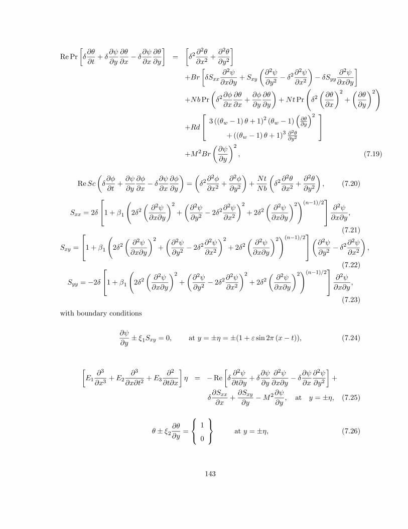
RePr
∙
+
−
¸=
∙22
2+
2
2
¸+
∙
2
+
µ2
2− 2
2
2
¶−
2
¸+Pr
µ2
+
¶+Pr
Ã2µ
¶2+
µ
¶2!
+
⎡⎣ 3 (( − 1) + 1)2 ( − 1)³
´2+(( − 1) + 1)3 2
2
⎤⎦+2
µ
¶2 (7.19)
Re
µ
+
−
¶=
µ22
2+
2
2
¶+
µ22
2+
2
2
¶ (7.20)
= 2
⎡⎣1 + 1
Ã22
µ2
¶2+
µ2
2− 22
2
2
¶2+ 22
µ2
¶2!(−1)2⎤⎦ 2
(7.21)
=
⎡⎣1 + 1
Ã22
µ2
¶2+
µ2
2− 22
2
2
¶2+ 22
µ2
¶2!(−1)2⎤⎦µ22− 2
2
2
(7.22)
= −2⎡⎣1 + 1
Ã22
µ2
¶2+
µ2
2− 22
2
2
¶2+ 22
µ2
¶2!(−1)2⎤⎦ 2
(7.23)
with boundary conditions
± 1 = 0, at = ± = ±(1 + sin 2 (− )) (7.24)
∙1
3
3+2
3
2+3
2
¸ = −Re
∙2
+
2
−
2
2
¸+
+
−2
at = ± (7.25)
± 2
=
⎧⎨⎩ 1
0
⎫⎬⎭ at = ± (7.26)
143

± 3
=
⎧⎨⎩ 1
0
⎫⎬⎭ at = ± (7.27)
The dimensionless parameters are
=
=
Re =
=
r
0 1 =
∗
³
´−1
=(1 − 0)
=
(1 − 0)
=
Pr =
=
2
(1 − 0) =
16∗ 303∗
=1
0
1 = − ∗3
3 2 =
∗3
3 3 =
∗13
2 (7.28)
Here depicts amplitude ratio, wave number, Re Reynolds number, Hartman number,
1 Sisko fluid parameter, Brownian motion parameter, thermophoresis parameter,
Schmidt number, Pr Prandtl number, Brinkman number, radiation parameter and 1
2 3 the compliant wall parameters.
Lubrication approach leads to
=
−2
(7.29)
= 0 (7.30)
0 =2
2+
2
2+Pr
+Pr
µ
¶2+2
µ
¶2+
"3 (( − 1) + 1)2 ( − 1)
µ
¶2+ (( − 1) + 1)3
2
2
# (7.31)
2
2+
2
2= 0 (7.32)
= 0 = (7.33)
=
⎡⎣1 + 1
õ2
2
¶2!(−1)2⎤⎦µ22
¶ (7.34)
144

with boundary conditions
± 1 = 0, at = ± = ±(1 + sin 2 (− )) (7.35)
∙1
3
3+2
3
2+3
2
¸ =
−2
at = ± (7.36)
± 2
=
⎧⎨⎩ 1
0
⎫⎬⎭ at = ± (7.37)
± 3
=
⎧⎨⎩ 1
0
⎫⎬⎭ at = ± (7.38)
The above mentioned system via NDSolve of Mathematica 9.0 is computed.
7.2.1 Expression for entropy generation
Mathematical expressions for viscous dissipation is
Φ =
+
+
µ
+
¶ (7.39)
Volumetric entropy generation in dimensional form is given by
000 =
2
õ
¶2+
µ
¶2+16∗
3∗
µ
¶2!| z
+20
2
| z
+Φ
|z
+
õ
¶2+
µ
¶2!+
µ
+
¶| z
(7.40)
In dimensionless form
=000
000
=³1 + (( − 1) + 1)3
´µ
¶2+
2
Λ
µ
¶2+
Λ
µ2
2
¶+
Λ
µ
¶µ
¶+
Λ2
µ
¶2 (7.41)
145
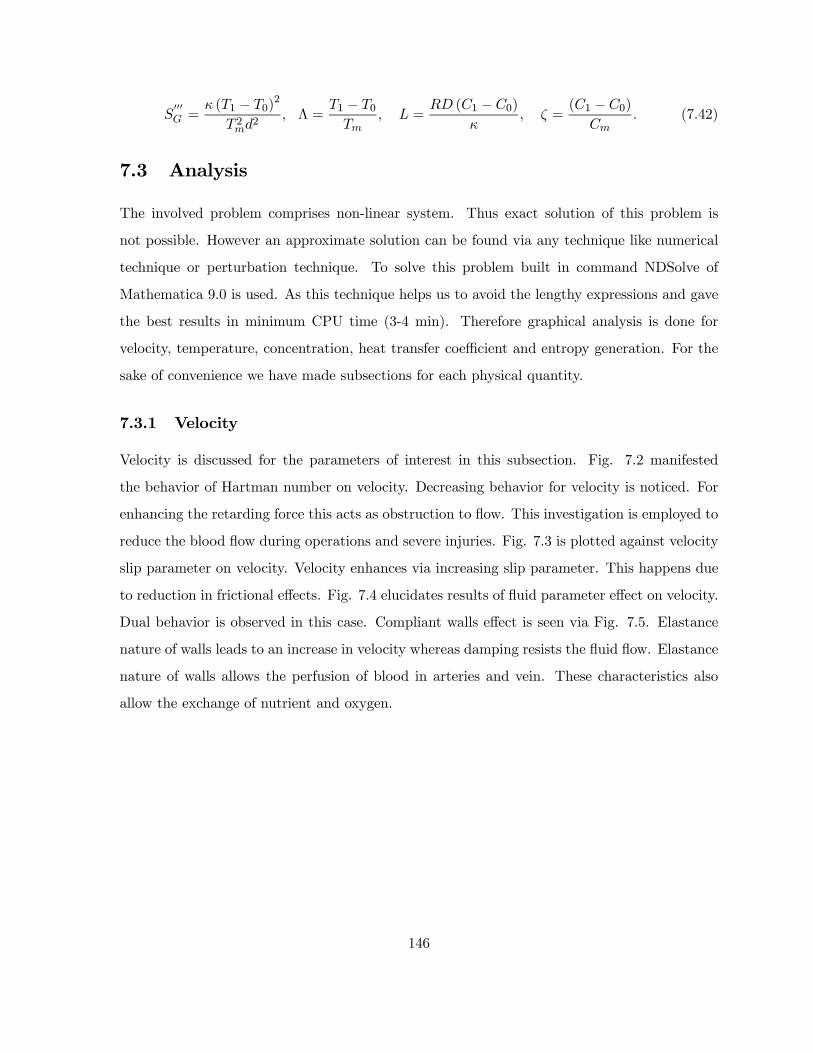
000 =
(1 − 0)2
22
Λ =1 − 0
=
(1 − 0)
=
(1 − 0)
(7.42)
7.3 Analysis
The involved problem comprises non-linear system. Thus exact solution of this problem is
not possible. However an approximate solution can be found via any technique like numerical
technique or perturbation technique. To solve this problem built in command NDSolve of
Mathematica 9.0 is used. As this technique helps us to avoid the lengthy expressions and gave
the best results in minimum CPU time (3-4 min). Therefore graphical analysis is done for
velocity, temperature, concentration, heat transfer coefficient and entropy generation. For the
sake of convenience we have made subsections for each physical quantity.
7.3.1 Velocity
Velocity is discussed for the parameters of interest in this subsection. Fig. 7.2 manifested
the behavior of Hartman number on velocity. Decreasing behavior for velocity is noticed. For
enhancing the retarding force this acts as obstruction to flow. This investigation is employed to
reduce the blood flow during operations and severe injuries. Fig. 7.3 is plotted against velocity
slip parameter on velocity. Velocity enhances via increasing slip parameter. This happens due
to reduction in frictional effects. Fig. 7.4 elucidates results of fluid parameter effect on velocity.
Dual behavior is observed in this case. Compliant walls effect is seen via Fig. 7.5. Elastance
nature of walls leads to an increase in velocity whereas damping resists the fluid flow. Elastance
nature of walls allows the perfusion of blood in arteries and vein. These characteristics also
allow the exchange of nutrient and oxygen.
146

Fig. 7.2 Fig. 7.3
72 via change in when 1 = 002 2 = 001 3 = 001 = 01 = 02 = 02
= 15 1 = 001 2 = 001 3 = 001 = 01 = 01 1 = 02 = 15 = 20
= 05 = 11
73 via change in 1 when 1 = 002 2 = 001 3 = 001 = 01 = 02 = 02
= 15 2 = 001 3 = 001 = 01 = 01 1 = 02 = 15 = 20 = 01
= 05 = 11
Fig. 7.4 Fig. 7.5
74 via change in 1 when 1 = 002 2 = 001 3 = 001 = 01 = 02 = 02
147

= 15 1 = 001 2 = 001 3 = 001 = 01 = 01 = 15 = 20 = 01
= 05 = 11
75 via change in 1 2 and 3 when = 01 = 02 = 02 = 15 1 = 001
2 = 001 3 = 001 = 01 = 01 1 = 02 = 15 = 20 = 01 = 05
= 11
7.3.2 Temperature
Temperature behavior for pertinent parameters is discussed via Figs. 7.6-7.14. Fig. 7.6 in-
dicated that for larger Hartman number, tends to increase at center of channel in view of
Joule heating effects. Fig. 7.7 is drawn for the sake of Brownian motion effects on tempera-
ture. Increasing Brownian motion parameter leads to higher temperature. Random motion of
the particles elevated the kinetic energy and molecular vibrations. Hence rise in is verified.
Moreover thermophoresis () on shows the same behavior (see Fig. 7.8). Thermal slip result
on is notified through Fig. 7.9. It is clearly seen via this Fig. that thermal slip parameter
leads to an enhancement in temperature. As slip reduces the friction and hence rise in velocity
and in temperature. Fig. 7.10 demonstrates fluid parameter behavior. Here temperature is
increasing. Figs. 7.11 and 7.12 display the radiation parameter and Brinkman number impacts
on Reverse behavior is seen for both cases. Basically Brinkman number measures the heat
loss due to viscous dissipation. This includes the conversion in internal energy results in heating
up the fluid. So temperature rises for more heat loss. Fig. 7.13 portrayed the influence of
on temperature. Result show that decay is observed in this case. Fig. 7.14 is drawn for 0
( = 1−3) influence on temperature. Here 1 and 2 tend to increase the temperature whereas3 leads to decay of temperature. Reason can be linked with velocity in view of kinetic theory.
148

Fig. 7.6 Fig. 7.7
76 via change in when 1 = 002 2 = 001 3 = 001 = 01 = 02 = 02
= 15 1 = 001 2 = 001 3 = 001 = 01 = 01 1 = 02 = 15 = 20
= 05 = 11
77 via change in when 1 = 002 2 = 001 3 = 001 = 01 = 02 = 02
= 15 1 = 001 2 = 001 3 = 001 = 01 1 = 02 = 15 = 20 = 01
= 05 = 11
Fig. 7.8 Fig. 7.9
78 via change in when 1 = 002 2 = 001 3 = 001 = 01 = 02 = 02
149

= 15 1 = 001 2 = 001 3 = 001 = 01 1 = 02 = 15 = 20 = 01
= 05 = 11
79 via change in 2 when 1 = 002 2 = 001 3 = 001 = 01 = 02 = 02
= 15 1 = 001 3 = 001 = 01 = 01 1 = 02 = 15 = 20 = 01
= 05 = 11
Fig. 7.10 Fig. 7.11
710 via change in 1 when 1 = 002 2 = 001 3 = 001 = 01 = 02 = 02
= 15 1 = 001 2 = 001 3 = 001 = 01 = 01 = 15 = 20 = 01
= 05 = 11
711 via change in when 1 = 002 2 = 001 3 = 001 = 01 = 02 = 02
= 15 1 = 001 2 = 001 3 = 001 = 01 = 01 1 = 02 = 15 = 20
= 01 = 11
150

Fig. 7.12 Fig. 7.13
712 via change in when 1 = 002 2 = 001 3 = 001 = 01 = 02 = 02
= 15 1 = 001 2 = 001 3 = 001 = 01 = 01 1 = 02 = 15 = 01
= 05 = 11
713 via change in when 1 = 002 2 = 001 3 = 001 = 01 = 02 = 02
= 15 1 = 001 2 = 001 3 = 001 = 01 = 01 1 = 02 = 15 = 20
= 01 = 05
Fig. 7.14
714 via change in 1 2 and 3 when = 01 = 02 = 02 = 15 1 = 001
151

2 = 001 3 = 001 = 01 = 01 1 = 02 = 15 = 20 = 01 = 05
= 11
7.3.3 Nanoparticle concentration
This subsection contains the information about concentration under the influences of embedded
parameters of interest. Fig. 7.15 is prepared for the sake of concentration slip parameter on
It is seen that an enhancement in concentration slip parameter leads to decay in concentration.
Fig. 7.16 reveals the result that enhancement in give rise to Figs. 7.17 and 7.18 display
decreasing behavior of radiation parameter () and thermophoresis parameter () respec-
tively. Fig. 7.18 displayed opposite behavior when compared with temperature. Brownian
motion parameter result on is seen opposite than (see Fig. 7.19). For increasing the
random motion of the particles enhances and rise in concentration is observed. Wall parameters
display decay for elastance parameters whereas enhancement is observed for damping variable
(see Fig. 7.20).
Fig. 7.15 Fig. 7.16
715 via change in 3 when 1 = 002 2 = 001 3 = 001 = 01 = 02 = 01
= 15 1 = 001 2 = 001 = 01 = 01 1 = 02 = 15 = 20 = 01
= 05 = 11
716 via change in when 1 = 002 2 = 001 3 = 001 = 01 = 02 = 01
152
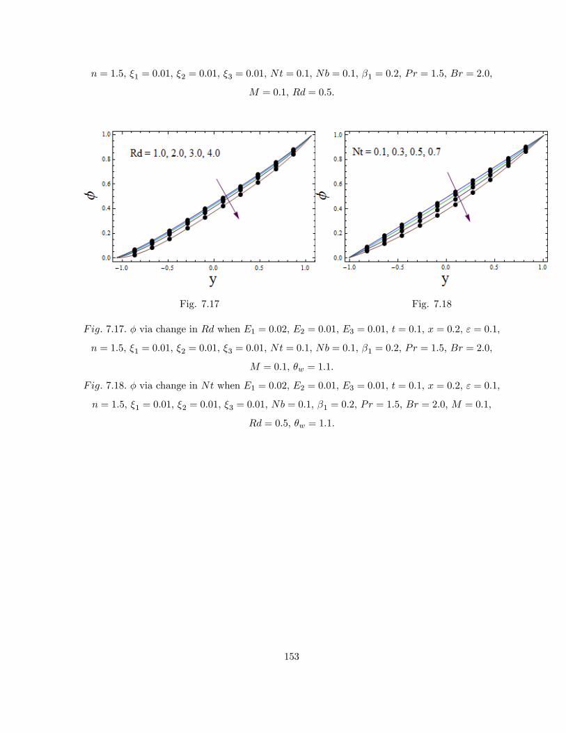
= 15 1 = 001 2 = 001 3 = 001 = 01 = 01 1 = 02 = 15 = 20
= 01 = 05
Fig. 7.17 Fig. 7.18
717 via change in when 1 = 002 2 = 001 3 = 001 = 01 = 02 = 01
= 15 1 = 001 2 = 001 3 = 001 = 01 = 01 1 = 02 = 15 = 20
= 01 = 11
718 via change in when 1 = 002 2 = 001 3 = 001 = 01 = 02 = 01
= 15 1 = 001 2 = 001 3 = 001 = 01 1 = 02 = 15 = 20 = 01
= 05 = 11
153

Fig. 7.19 Fig. 7.20
719 via change in when 1 = 002 2 = 001 3 = 001 = 01 = 02 = 01
= 15 1 = 001 2 = 001 3 = 001 = 01 1 = 02 = 15 = 20 = 01
= 05 = 11
720 via change in 1 2 and 3 when 1 = 002 2 = 001 3 = 001 = 01
= 02 = 01 = 15 1 = 001 2 = 001 3 = 001 = 01 = 01 1 = 02
= 15 = 20 = 01 = 05 = 11
7.3.4 Entropy generation analysis
In this subsection the analysis of entropy generation is presented for pertinent parameters of
interest. Fig. 7.21 is drawn for the analysis of entropy generation in view of Hartman number.
Entropy increases near center of channel in view of Joule heating. and behaviors on
entropy are observed via Figs. 7.22 and 7.23. Both cases show enhancement as in case of
temperature. Enhancement in kinetic energy of the particles create more disorderliness. Fig.
7.24 elucidates radiation parameter results on entropy. Radiation caused enhancement in the
disorderedness. Fig. 7.25 illustrates that larger values of tend to decrease in entropy. For
larger values of concentration difference parameter () Fig. 7.26 is plotted. Enhancement is
observed in this case. Influence of diffusion coefficient parameter on is viewed via Fig. 7.27.
Entropy is an increasing function of An increase in causes decrease of thermal conductivity.
154

It shows an increase in temperature and entropy. Temperature difference parameter leads to
decay in entropy (see Fig. 7.28). Thermal slip effect on entropy is plotted against Fig. 7.29.
Results reveals decaying behavior here.
Fig. 7.21 Fig. 7.22
721 via change in when 1 = 002 2 = 001 3 = 001 = 01 = 02
= 02 = 15 1 = 001 2 = 001 3 = 001 = 01 = 01 1 = 02 = 15
= 20 = 05 = 11 Λ = 05 = 05 = 05
722 via change in when 1 = 002 2 = 001 3 = 001 = 01 = 02
= 02 = 15 1 = 001 2 = 001 3 = 001 = 01 1 = 02 = 15 = 20
155

= 01 = 05 = 11 Λ = 05 = 05 = 05
Fig. 7.23 Fig. 7.24
723 via change in when 1 = 002 2 = 001 3 = 001 = 01 = 02
= 02 = 15 1 = 001 2 = 001 3 = 001 = 01 1 = 02 = 15 = 20
= 01 = 05 = 11 Λ = 05 = 05 = 05
724 via change in when 1 = 002 2 = 001 3 = 001 = 01 = 02
= 02 = 15 1 = 001 2 = 001 3 = 001 = 01 = 01 1 = 02 = 15
= 20 = 01 = 11 Λ = 05 = 05 = 05
Fig. 7.25 Fig. 7.26
725 via change in when 1 = 002 2 = 001 3 = 001 = 01 = 02
156

= 02 = 15 1 = 001 2 = 001 3 = 001 = 01 = 01 1 = 02 = 15
= 20 = 01 = 05 Λ = 05 = 05 = 05
726 via change in when 1 = 002 2 = 001 3 = 001 = 01 = 02 = 02
= 15 1 = 001 2 = 001 3 = 001 = 01 = 01 1 = 02 = 15 = 20
= 01 = 05 = 11 Λ = 05 = 05
Fig. 7.27 Fig. 7.28
727 via change in when 1 = 002 2 = 001 3 = 001 = 01 = 02
= 02 = 15 1 = 001 2 = 001 3 = 001 = 01 = 01 1 = 02 = 15
= 20 = 01 = 05 = 11 Λ = 05 = 05
728 via change in Λ when 1 = 002 2 = 001 3 = 001 = 01 = 02
= 02 = 15 1 = 001 2 = 001 3 = 001 = 01 = 01 1 = 02 = 15
= 20 = 01 = 05 = 11 = 05 = 05
157

Fig. 7.29
729 via change in 2 when 1 = 002 2 = 001 3 = 001 = 01 = 02
= 02 = 15 1 = 001 3 = 001 = 01 = 01 1 = 02 = 15 = 20
= 01 = 05 = 11 Λ = 05 = 05 = 05
7.3.5 Heat transfer coefficient
Plots for heat transfer coefficient are drawn through Figs. 7.30-7.35. Fig. 7.30 represents the
behavior. Heat transfer coefficient decreases via . Results for and can be seen via
Figs. 7.31 and 7.32. Decay in heat transfer coefficient are seen. Radiation parameter portrayed
an enhancement in (see Fig. 7.33). Thermal slip parameter caused reduction in whereas
walls parameters results are qualitatively similar to temperature (see Figs. 7.34 and 7.35).
158

Fig. 7.30 Fig. 7.31
730 via change in when 1 = 002 2 = 001 3 = 001 = 01 = 02 = 15
1 = 001 2 = 001 3 = 001 = 01 = 01 1 = 02 = 15 = 20 = 05
= 11
731 via change in when 1 = 002 2 = 001 3 = 001 = 01 = 02
= 15 1 = 001 2 = 001 3 = 001 = 01 1 = 02 = 15 = 20 = 01
= 05 = 11
Fig. 7.32 Fig. 7.33
732 via change in when 1 = 002 2 = 001 3 = 001 = 01 = 02 = 15
159
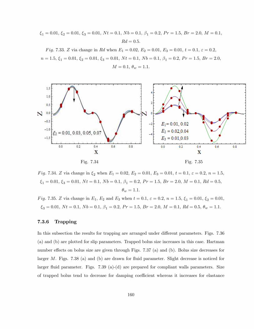
1 = 001 2 = 001 3 = 001 = 01 = 01 1 = 02 = 15 = 20 = 01
= 05
733 via change in when 1 = 002 2 = 001 3 = 001 = 01 = 02
= 15 1 = 001 2 = 001 3 = 001 = 01 = 01 1 = 02 = 15 = 20
= 01 = 11
Fig. 7.34 Fig. 7.35
734 via change in 2 when 1 = 002 2 = 001 3 = 001 = 01 = 02 = 15
1 = 001 3 = 001 = 01 = 01 1 = 02 = 15 = 20 = 01 = 05
= 11
735 via change in 1 2 and 3 when = 01 = 02 = 15 1 = 001 2 = 001
3 = 001 = 01 = 01 1 = 02 = 15 = 20 = 01 = 05 = 11
7.3.6 Trapping
In this subsection the results for trapping are arranged under different parameters. Figs. 7.36
(a) and (b) are plotted for slip parameters. Trapped bolus size increases in this case. Hartman
number effects on bolus size are given through Figs. 7.37 (a) and (b). Bolus size decreases for
larger . Figs. 7.38 (a) and (b) are drawn for fluid parameter. Slight decrease is noticed for
larger fluid parameter. Figs. 7.39 (a)-(d) are prepared for compliant walls parameters. Size
of trapped bolus tend to decrease for damping coefficient whereas it increases for elastance
160

coefficients.
Fig. 7.36 (a). (b)
736 via change in 1 when 1 = 002 2 = 001 3 = 001 = 00 = 02 = 15
2 = 001 3 = 001 = 01 = 01 1 = 02 = 15 = 20 = 01 = 05
= 11 () 1 = 001 () 1 = 003
Fig. 7.37 (a) (b)
161
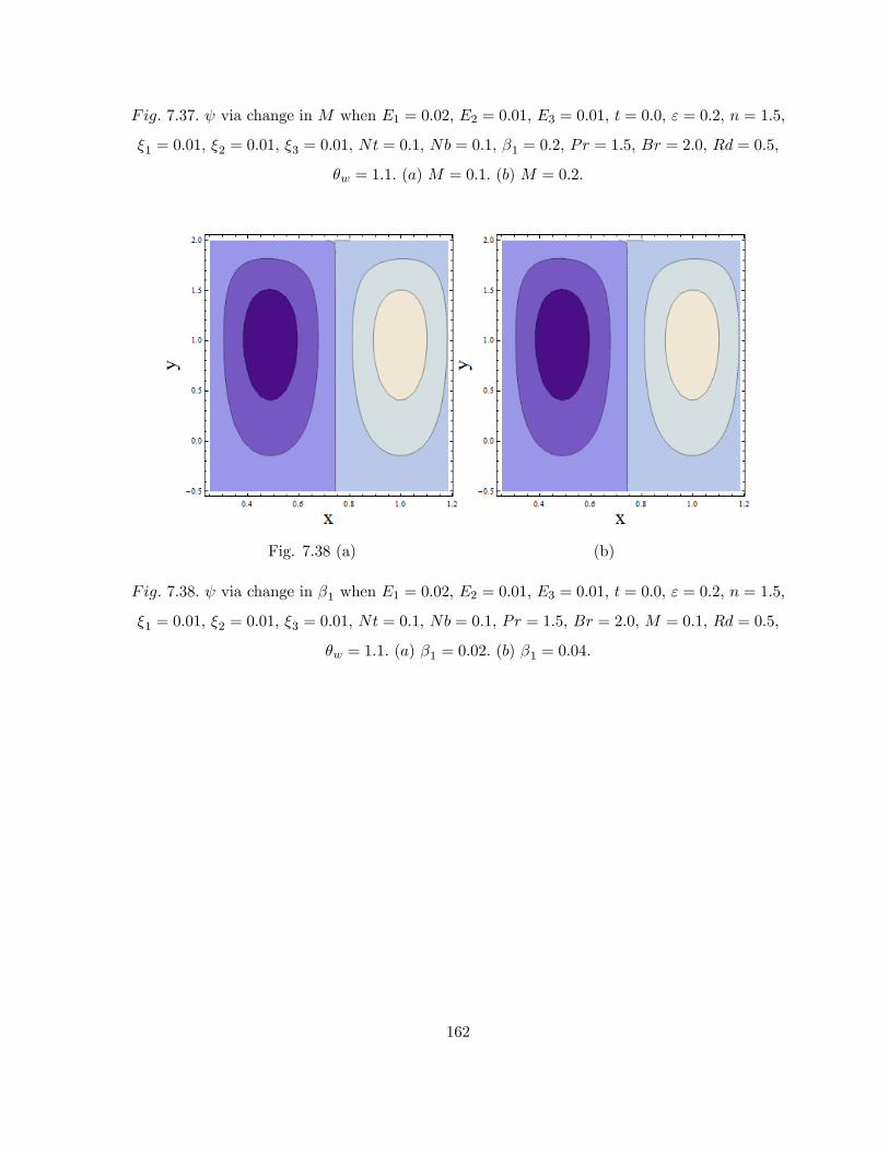
737 via change in when 1 = 002 2 = 001 3 = 001 = 00 = 02 = 15
1 = 001 2 = 001 3 = 001 = 01 = 01 1 = 02 = 15 = 20 = 05
= 11 () = 01 () = 02
Fig. 7.38 (a) (b)
738 via change in 1 when 1 = 002 2 = 001 3 = 001 = 00 = 02 = 15
1 = 001 2 = 001 3 = 001 = 01 = 01 = 15 = 20 = 01 = 05
= 11 () 1 = 002 () 1 = 004
162

Fig. 7.39 (a) (b)
(c) (d)
739 via change in 1 2 3 when = 00 = 02 = 15 1 = 001 2 = 001
3 = 001 = 01 = 01 1 = 02 = 15 = 20 = 01 = 05 = 11
() 1 = 002 2 = 001 3 = 001 () 1 = 003 2 = 001 3 = 001 () 1 = 002
2 = 003 3 = 001 () 1 = 002 2 = 001 3 = 002
163

7.3.7 Validation of problem
Fig. 7.40
740 via change in and when 1 = 001 2 = 002 3 = 001 = 01 = 02
= 02 1 = 01 2 = 01 3 = 01 1 = 0 = 10 = 10 = 0 = 0
This Fig. is sketched for the effect of Brownian motion and thermophoresis parameter on
temperature which validates our results. In our problem we have taken 1 = 0 = 0 = 0
and get the result of study by Mustafa et. al. [170]. In this study the authors have taken the
nanofluid, slip conditions and wall properties. They solved the problem by using homotopy
analysis method (HAM). We observed that our results are in good agreement with limiting
results of [170].
7.4 Conclusions
Key observations of present chapter are mentioned below.
• Velocity slip and Hartman number have opposite behaviors for velocity.
• Influences of and on temperature are similar.
• Radiation parameter and Brinkman number have opposite results on fluid temperature.
• Concentration slip parameter leads to decay in concentration.
164

• Entropy enhancement is noted for concentration difference and diffusion coefficient para-meters.
• Radiation parameter and thermal slip parameter results on are opposite.
• Bolus size increases with larger slip parameter.
165

Chapter 8
Entropy generation and endoscopic
effects on peristalsis with modified
Darcy’s law
8.1 Introduction
Present chapter highlights the outcomes of endoscopy and entropy generation in MHD peri-
staltic flow of Sisko fluid. Unlike the traditional approach, the flow modeling for porous medium
is based upon modified Darcy’s law. Salient features of Joule heating and viscous dissipation
are investigated. Convective conditions for heat transfer are utilized. The problem after invok-
ing long wavelength approximation is numerically solved. Graphical analysis provides physical
insight. Graphs are plotted for velocity, temperature, entropy generation, Bejan number and
heat transfer coefficient for the pertinent parameters of interest. Results discloses that the
enhancement in Darcy number increases the fluid velocity and temperature. It also caused an
enhancement in entropy generation and Bejan number. Magnetic field leads to enhance the
temperature and entropy generation. Moreover the flexible wall parameters show increasing
trend for elastance coefficients whereas damping coefficient decays the fluid velocity.
166

8.2 Modeling
Here magnetohydrodynamic flow of Sisko fluid between two coaxial uniform tubes is considered.
Inner tube (at = 1) is fixed while the outer tube (at = 2) is subject to peristaltic wave
[213]
= 1 = (8.1)
= 2 = + sin2
( − ) (8.2)
Here and are radii of outer and inner tubes. Further wavelength, wave amplitude, wave speed
and time are symbolized as and respectively (see Fig. 8.1). Cylindrical coordinate (
) are selected such that along radial direction and perpendicular to . Viscous dissipation
and Ohmic heating are present.
Fig. 8.1: Flow Configuration
Fluid is electrically conducting using constant magnetic field. Electric field consideration is not
attended. Small magnetic Reynolds number leads to omission of induced magnetic field. In
addition incompressible Sisko fluid fills the porous space. Thus by modified Darcy’s law one
has for pressure drop [217]:
∇ = − κ1
³+ ∗
p|Π|−1
´V (8.3)
167

in which porosity and permeability of medium are κ and 1 respectively. Here and ∗ are
material constants. Keeping above expression in mind, the resistance satisfies [217]:
R = − κ1
³+ ∗
p|Π|−1
´V (8.4)
which in component form yields
= − κ1
³+ ∗
p|Π|−1
´ (8.5)
= − κ1
³+ ∗
p|Π|−1
´ (8.6)
where and are the velocities in and −directions. We have following expressions [124]:
+
+
= 0 (8.7)
µ
¶= −
+1
()
+
()
−
+ (8.8)
µ
¶= −
+1
()
+
()
− 20 + (8.9)
µ
¶=
µ2
2+1
+
2
2
¶+
+
+
+
µ
+
¶+20
2 (8.10)
In above equations represents the temperature. for density of fluid, and the
extra stress components, the pressure and the thermal conductivity.
Expression of for Sisko material is [72]:
S =³+ ∗
p|Π|−1
´A1 (8.11)
168
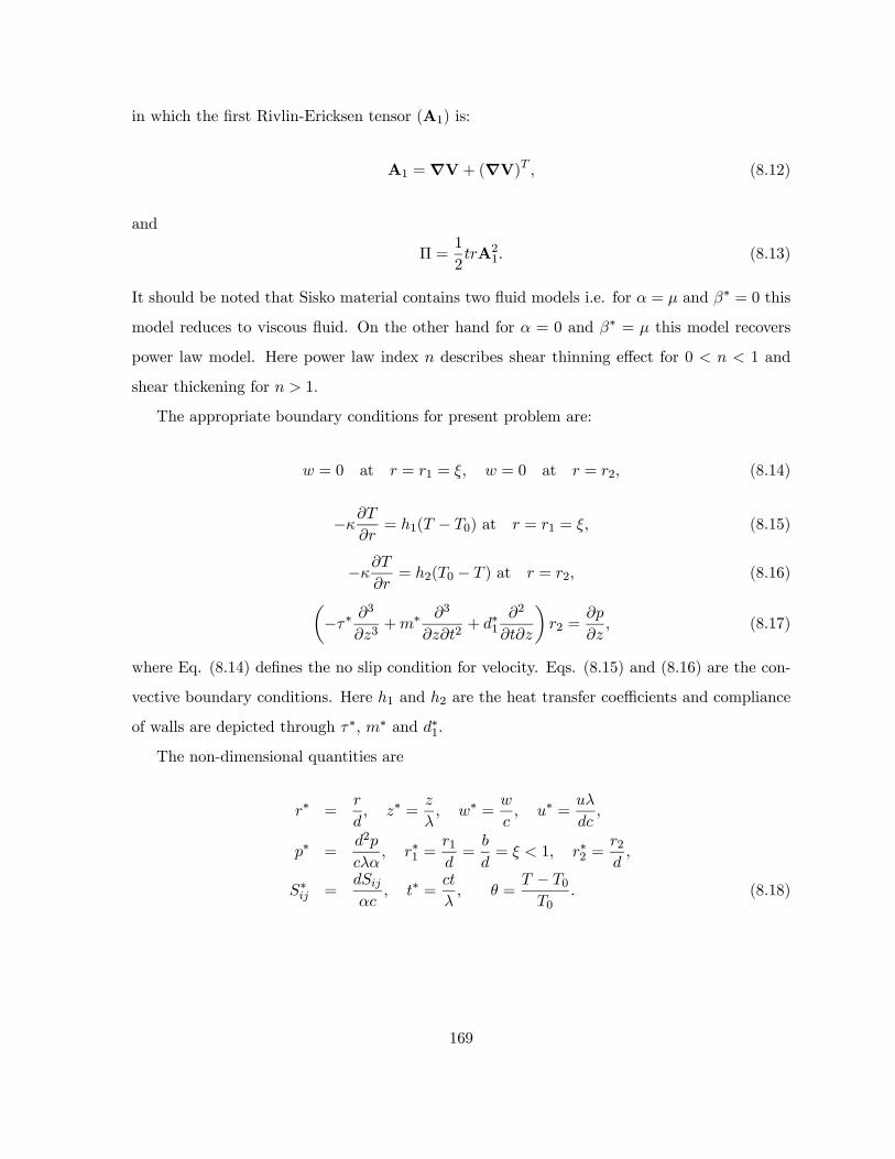
in which the first Rivlin-Ericksen tensor (A1) is:
A1 =∇V+ (∇V) (8.12)
and
Π =1
2A21 (8.13)
It should be noted that Sisko material contains two fluid models i.e. for = and ∗ = 0 this
model reduces to viscous fluid. On the other hand for = 0 and ∗ = this model recovers
power law model. Here power law index describes shear thinning effect for 0 1 and
shear thickening for 1
The appropriate boundary conditions for present problem are:
= 0 at = 1 = = 0 at = 2 (8.14)
−
= 1( − 0) at = 1 = (8.15)
−
= 2(0 − ) at = 2 (8.16)µ−∗
3
3+∗
3
2+ ∗1
2
¶2 =
(8.17)
where Eq. (8.14) defines the no slip condition for velocity. Eqs. (8.15) and (8.16) are the con-
vective boundary conditions. Here 1 and 2 are the heat transfer coefficients and compliance
of walls are depicted through ∗, ∗ and ∗1.
The non-dimensional quantities are
∗ =
∗ =
∗ =
∗ =
∗ =2
∗1 =
1
=
= 1 ∗2 =
2
∗ =
∗ =
=
− 0
0 (8.18)
169

Non-dimensionlized form of system is
Re 3µ
+
+
¶= −
+
()
+ 2
()
− 2
³1 + 1
p|Π|−1
´−
(8.19)
Re
µ
+
+
¶= −
+1
()
+
()
− 1
³1 + 1
p|Π|−1
´ −2
(8.20)
RePr
µ
+
+
¶=
µ2
2+1
+ 2
2
2
¶+22
+
+
+
+
µ
+
¶ (8.21)
= 0 at = 1 = = 0 at = 2 (8.22)
+1 = 0 at = 1 = (8.23)
−2 = 0 at = 2 (8.24)
∙1
3
3+2
3
2+3
2
¸2 =
1
()
+
()
−Re
µ
+
+
¶− 1
³1 + 1
p|Π|−1
´
−2 at = 1 = and = 2(8.25)
with
Re =
=
r
0 Pr =
=2
0 = Pr =
1
2κ =
1 =∗
³
´−1 1 =
1
2 =
2
1 = − ∗3
3 2 =
∗3
3 3 =
∗13
2 (8.26)
Here Re depicts Reynolds number, the Hartman number, Pr the Prandtl number, the
170

Eckert number, (product of Eckert and Prandtl numbers) the Brinkman number, the
Darcy number, the wave number, 1 the fluid parameter, 0 ( = 1 2) the Biot numbers
and 0 ( = 1− 3) the compliance wall parameter.Definition of stream function is
= −1
=
1
(8.27)
Employing above expression and lubrication approach we arrive at
= 0 (8.28)
=1
()
− 2
− 1
Ã1 + 1
µ1
2
2− 1
2
¶−1!µ1
¶ (8.29)
2
2+1
+
µ1
2
2− 1
2
¶+
2
2
µ
¶2= 0 (8.30)
=
Ã1 + 1
µ1
2
2− 1
2
¶−1!µ1
2
2− 1
2
¶ (8.31)
= 0 at = 1 =
= 0 at = 2 (8.32)
+1 = 0 at = 1 = (8.33)
−2 = 0 at = 2 (8.34)
1
()
− 1
Ã1 + 1
µ1
2
2− 1
2
¶−1!µ1
¶− 2
=
∙1
3
3+2
3
2+3
2
¸2 at = 1 = and = 2 (8.35)
where incompressibility condition is automatically justified. From Eqs. (8.28) and (8.29), one
can write
"1
()
− 2
− 1
Ã1 + 1
µ1
2
2− 1
2
¶−1!µ1
¶#= 0 (8.36)
171
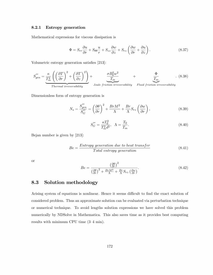
8.2.1 Entropy generation
Mathematical expressions for viscous dissipation is
Φ =
+
+
+
µ
+
¶ (8.37)
Volumetric entropy generation satisfies [213]:
000 =
2
õ
¶2+
µ
¶2!| z
+20
2
| z
+Φ
|z
(8.38)
Dimensionless form of entropy generation is
=000
000
=
µ
¶2+
2
Λ+
Λ
µ
¶ (8.39)
000 =
20 2
2 Λ =
0
(8.40)
Bejan number is given by [213]:
=
(8.41)
or
=
¡
¢2¡
¢2+ 2
Λ+
Λ
¡
¢ (8.42)
8.3 Solution methodology
Arising system of equations is nonlinear. Hence it seems difficult to find the exact solution of
considered problem. Thus an approximate solution can be evaluated via perturbation technique
or numerical technique. To avoid lengths solution expressions we have solved this problem
numerically by NDSolve in Mathematica. This also saves time as it provides best computing
results with minimum CPU time (3—4 min).
172

8.4 Analysis
This section contains information about graphical interpretation of the results. We firstly
discuss the velocity function for Darcy number (), Hartman number (), fluid parameter
(1) and compliant wall parameters ( = 1− 3) Fig. 8.2 (a) depicts influence on velocity.
Velocity is an increasing function of . Obviously more pores aid the flow speed. Fig. 8.2 (b)
is plotted for velocity against As expected the applied magnetic field provides a reduction in
velocity. This is because of enhancement in resistive force offered to fluid. Fig. 8.2 (c) witnesses
dual behavior of velocity for material parameter. Compliant nature is discussed via Fig. 8.2
(d). An enhancement in velocity is observed for 1 and 2 whereas damping force leads to
decrease of velocity. This situation in quite useful in blood perfusion process in arteries and
veins.
(a) (b)
173

(c) (d)
82 Plots for velocity when 1 = 002 2 = 001 3 = 001 = 01 = 02 = 02
= 05 = 10 = 02 1 = 02 1 = 8 2 = 10 = 40(a) effect on (b)
effect on (c) 1 effect on (d) 1 2 3 effects on
Temperature for different parameters is discussed via Figs. 3 (a-f). These Figs. include
the influences of Darcy number () Brinkman number () Hartman number () fluid
parameter (1) and Biot numbers (0). Fig. 8.3 (a) elucidates the results for increasing
values of Darcy number. Temperature is enhanced for . As higher values of lead to
more permeability which gave rise to the velocity of the fluid and as a result heat generation is
possible. Hence the temperature of the fluid rises. Fig. 8.3 (b) depicts temperature variation
for Brinkman number. Results reveal that temperature is an increasing function of . This
happens in view of viscous dissipation effect. Hartman number () shows an enhancement of
temperature (see Fig. 8.3 (c)). Joule heating aspect is responsible for this act. Behavior of fluid
parameter on thermal field is qualitatively similar to that of velocity (see Fig. 8.3 (d)). Biot
numbers results on temperature are demonstrated through Figs. 8.3 (e) and (f). Temperature
is enhanced for both Biot numbers.
174

(a) (b)
(c) (d)
175
(e) (f)
83 Plots for temperature when 1 = 002 2 = 001 3 = 001 = 01 = 02
= 02 = 05 = 10 = 02 1 = 02 1 = 8 2 = 10 = 40(a) effect on
(b) effect on (c) effect on (d) 1 effect on (e) 1 effect on (f) 2 effect on
Figs. 8.3 (a-d) have been prepared for examination of entropy generation. Fig. 8.4 (a)
declared that Darcy number () leads to an enhancement in entropy generation. As more
heat is produced with increase in permeability, that corresponds to more disorderliness. Fig.
8.4 (b) illustrated the results of Hartman number (). Here larger give rise to entropy
generation. It is because of the fact that temperature is directly related to . Brinkman
number influence on entropy generation is portrayed via Fig. 8.4 (c). Graphical analysis leads
to the fact that enhancement in entropy generation is observed in presence of viscous dissipation.
Fig. 8.4 (d) displayed the result of entropy generation through Λ. Reduction in is noticed
for larger Λ
176

(a) (b)
(c) (d)
84 Plots for entropy generation when 1 = 002 2 = 001 3 = 001 = 01 = 02
= 02 = 05 = 10 = 02 1 = 02 1 = 8 2 = 10 Λ = 05 = 10(a)
effect on (b) effect on (c) effect on (d) Λ effect on
Variation of Bejan number () for sundry variables is shown in the Figs. 8.5 (a-d). Fig.
8.5 (a) is prepared for impact of Darcy number on . Enhancement is seen for Bejan number
for larger Fig. 8.5 (b) is plotted for Brinkman number. It is noted that larger caused
an enhancement in Opposite results for and Λ are seen for Bejan number (see Figs. 8.5
(c) and (d)). Here Bejan number enhancement in fact means that heat transfer irreversibility
177

is high when compared with total heat transfer irreversibility.
(a) (b)
(c) (d)
85 Plots for Bejan number when 1 = 002 2 = 001 3 = 001 = 01 = 02
= 02 = 05 = 10 = 02 1 = 02 1 = 8 2 = 10 Λ = 05 = 10(a)
effect on (b) effect on (c) effect on (d) Λ effect on
Figs. 8.6 (a—e) capture the results of heat transfer coefficient. Fig. 8.6 (a) is arranged for
Darcy number. Here larger reveal an enhancement in heat transfer coefficient. Brinkman
number outcome is seen through Fig. 8.6 (b). Clearly heat transfer coefficient is increased for
Brinkman number. Heat transfer coefficient has decreasing impact for (see Fig. 8.6 (c)).
178

Biot numbers have opposite behavior for heat transfer coefficient (see Figs. 8.6 (d) and (e)).
(a) (b)
(c) (d)
179
(e)
86 Plots for heat transfer coefficient when 1 = 002 2 = 001 3 = 001 = 01
= 02 = 05 = 10 = 02 1 = 02 1 = 8 2 = 10 = 10(a) effect on
(b) effect on (c) effect on (c) 1 effect on (d) 2 effect on
Now we display streamlines for trapping phenomenon. Figs. 8.7 (a , b) describe the Hartman
number influence on bolus size. It is noted that size of trapped bolus reduces for larger strength
of applied magnetic field. Figs. 8.8 (a , b) are plotted for impact of on size of trapped
bolus. Bolus size shows an increase for larger Figs. 8.9 (a , b) illustrate that bolus size is
an increasing function of fluid parameter.
180

(a) (b)
87 effect on when 1 = 0002 2 = 0001 3 = 001 = 0 = 02 = 02
= 05 1 = 002 1 = 2 2 = 3 = 10 () = 10 () = 30
(a) (b)
88 effect on when 1 = 0002 2 = 0001 3 = 001 = 0 = 02 = 05
= 10 1 = 002 1 = 2 2 = 3 = 10 () = 01 () = 02
181
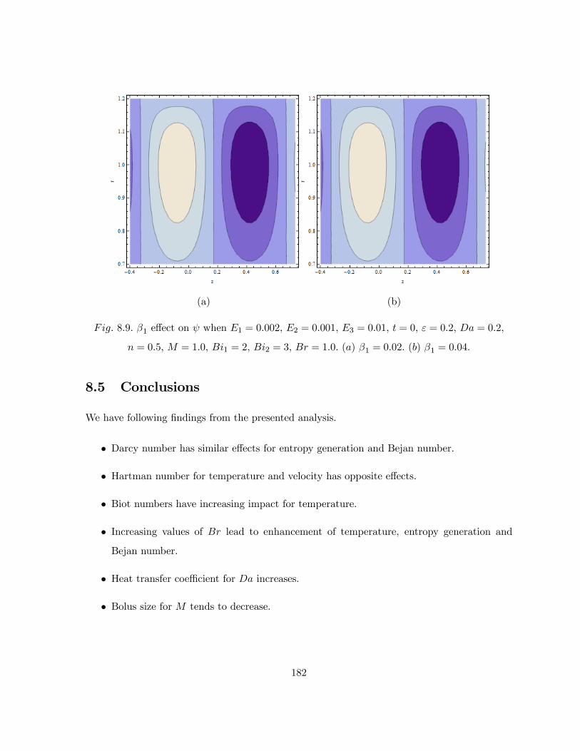
(a) (b)
89 1 effect on when 1 = 0002 2 = 0001 3 = 001 = 0 = 02 = 02
= 05 = 10 1 = 2 2 = 3 = 10 () 1 = 002 () 1 = 004
8.5 Conclusions
We have following findings from the presented analysis.
• Darcy number has similar effects for entropy generation and Bejan number.
• Hartman number for temperature and velocity has opposite effects.
• Biot numbers have increasing impact for temperature.
• Increasing values of lead to enhancement of temperature, entropy generation andBejan number.
• Heat transfer coefficient for increases.
• Bolus size for tends to decrease.
182

Chapter 9
Entropy optimization for peristalsis
of Rabinowitsch nanomaterial
9.1 Introduction
This chapter models peristaltic activity of Rabinowitsch material in a compliant walls channel.
Energy equation is accounted in presence of viscous dissipation and heat source/sink. Chem-
ical reaction is included in concentration expression. Nanomaterial characteristics are due to
Brownian motion and thermophoresis. Slip condition are utilized for velocity, temperature and
concentration. Exact solution is obtained for velocity. Further NDSolve is utilized for the
graphical analysis of temperature, concentration, entropy and heat transfer coefficient at the
wall. Results are also analyzed for viscous, shear thickening and shear thinning fluids. This
study reveals that the shear thinning fluids move with higher velocity than the viscous and shear
thickening fluids. Similarly temperature and entropy generation are also higher for shear thin-
ning case when compared with others. Further heat source parameter enhances the temperature
whereas sink parameter leads to decay. Slip parameter for velocity and temperature caused an
increase in the respective velocity and temperature. Moreover chemical reaction parameter
leads to enhancement in temperature and entropy generation for viscous, shear thickening and
shear thinning fluids. However shear thinning fluids are found prominent.
183

9.2 Problem formulation
We have an interest to examine peristaltic flow of Rabinowitsch liquid in a symmetric channel
with compliant boundaries. The walls are maintained at temperature 0 Brownian motion and
thermophoresis are discussed. Heat generation/absorption and chemical reaction are attended.
The partial slip constraints for velocity, temperature and concentration are studied. Flow is
due to travelling wave along the channel walls. Wall form is
= ± ( ) = ±∙+ sin
2
(− )
¸ (9.1)
where we take the channel width 2 wave amplitude speed wavelength This phenomenon
is shown via Fig. 9.1.
Fig. 9.1: Schematic Diagram
Flow problem is governed by the expressions [91, 108]
+
= 0 (9.2)
+
+
= − 1
+1
+1
(9.3)
+
+
= − 1
+1
+1
(9.4)
184
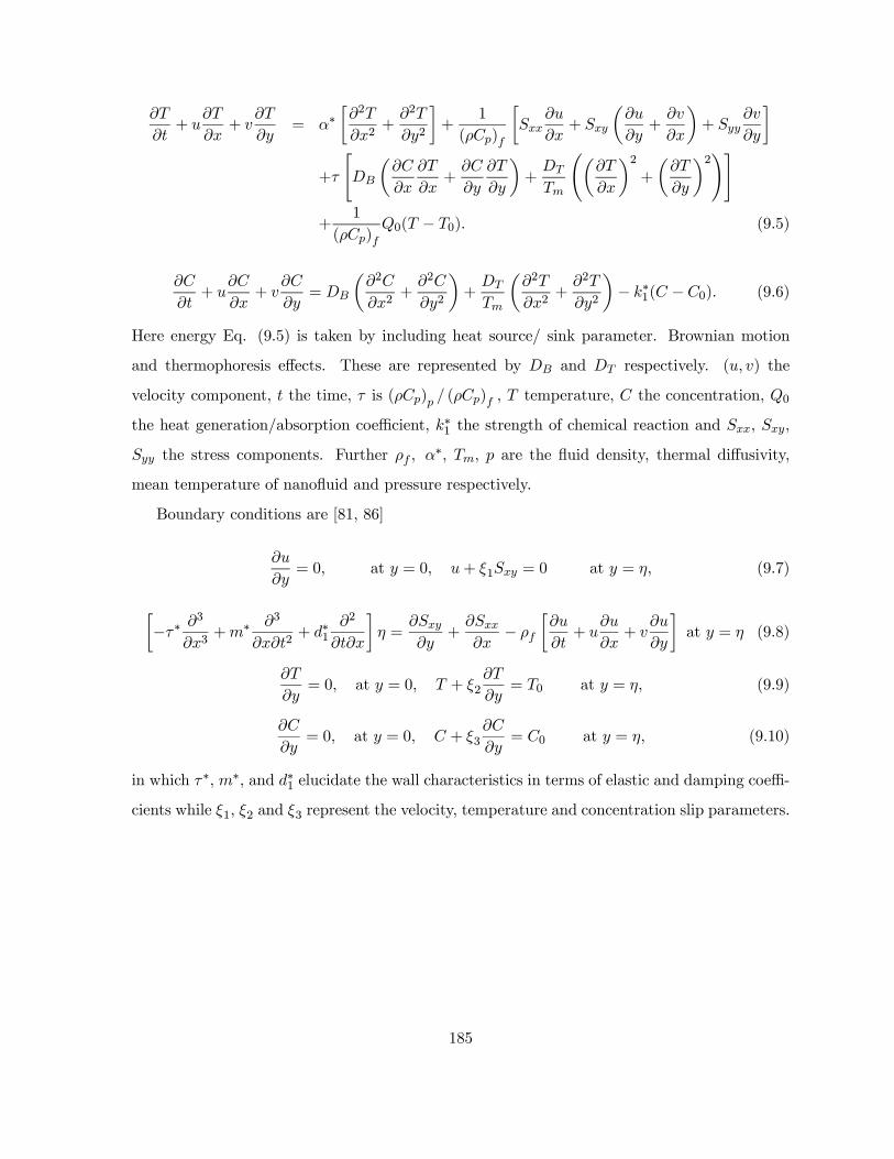
+
+
= ∗
∙2
2+
2
2
¸+
1
()
∙
+
µ
+
¶+
¸+
"
µ
+
¶+
õ
¶2+
µ
¶2!#+
1
()0( − 0) (9.5)
+
+
=
µ2
2+
2
2
¶+
µ2
2+
2
2
¶− ∗1( −0) (9.6)
Here energy Eq. (9.5) is taken by including heat source/ sink parameter. Brownian motion
and thermophoresis effects. These are represented by and respectively. ( ) the
velocity component, the time, is () () temperature, the concentration, 0
the heat generation/absorption coefficient, ∗1 the strength of chemical reaction and
the stress components. Further ∗ are the fluid density, thermal diffusivity,
mean temperature of nanofluid and pressure respectively.
Boundary conditions are [81, 86]
= 0 at = 0 + 1 = 0 at = (9.7)
∙−∗
3
3+∗
3
2+ ∗1
2
¸ =
+
−
∙
+
+
¸at = (9.8)
= 0 at = 0 + 2
= 0 at = (9.9)
= 0 at = 0 + 3
= 0 at = (9.10)
in which ∗, ∗, and ∗1 elucidate the wall characteristics in terms of elastic and damping coeffi-
cients while 1 2 and 3 represent the velocity, temperature and concentration slip parameters.
185

Non-dimensional variables are
∗ =
∗ =
∗ =
∗ =
∗ =
∗1 =1
∗2 =
2 ∗3 =
3 ∗ =
∗ =
∗ =
2
=
−0
0 ∗ =
33
3
= − 0
0 =
= −
(9.11)
After invoking Eq. (9.11), our system of equations (9.3-9.6) reduce to
Re
∙2
+
2
−
2
2
¸= −
+
+
(9.12)
Re
∙−2
2
− 2
2
2+ 2
2
¸= −
+ 2
+
(9.13)
RePr
∙
+
−
¸=
∙22
2+
2
2
¸+
⎡⎣ 2
+
³22− 2
22
´−
2
⎤⎦+Pr
µ2
+
¶+
Pr
Ã2µ
¶2+
µ
¶2!+ (9.14)
Re
µ
+
−
¶=
µ22
2+
2
2
¶+
µ22
2+
2
2
¶− 1 (9.15)
with boundary conditions
2
2= 0 at = 0
+ 1 = 0, at = = (1 + sin 2 (− )) (9.16)
∙1
3
3+2
3
2+3
2
¸ = −Re
∙2
+
2
−
2
2
¸+
+
at = (9.17)
186

= 0 at = 0 + 2
= 0 at = (9.18)
= 0 at = 0 + 3
= 0 at = (9.19)
with
=
=
Re =
=
02
=0
=
0
Pr =
=
=
2
(1 − 0) 1 =
∗12
1 = − ∗3
3 2 =
∗3
3 3 =
∗13
2 (9.20)
Here denotes the stream function, the temperature, the concentration, amplitude ratio,
wave number, Re Reynolds number, heat source sink parameter, and the Brownian
motion and thermophoresis parameters, Pr Prandtl number, Schmidt number, Brinkman
number, 1 chemical reaction parameter and 1 2 3 the compliant wall parameters.
Invoking lubrication approach we obtain
=
(9.21)
= 0 (9.22)
0 =2
2+
2
2+Pr
+Pr
µ
¶2+ (9.23)
2
2+
2
2− 1 = 0 (9.24)
with boundary conditions
2
2= 0 at = 0
+ 1 = 0, at = = (1 + sin 2 (− )) (9.25)
∙1
3
3+2
3
2+3
2
¸ =
at = (9.26)
187

= 0 at = 0 + 2
= 0 at = (9.27)
= 0 at = 0 + 3
= 0 at = (9.28)
where
+ ()3 =
(9.29)
9.2.1 Solution of the problem
As in eq. (9.29) is in implicit form. To obtain an explicit expression we will make use of
eq. (9.21). By eq. (9.8) we can write:
=
∙−∗
3
3+∗
3
2+ ∗1
2
¸ (9.30)
This will be used to find
We will now solve eq. (9.21) subject to slip condition of velocity. We arrive at
() =
µ2 − 2
2
¶+
µ
¶3µ4 − 4
2
¶− 1
µ
¶(9.31)
The energy and concentration equations for nanofluid involve of thermophoresis and Brownian
motion effects. To tackle these equations we have utilized the NDSolve technique in Math-
ematica. This algorithm gives the solutions in less computation time and avoid the lengthy
expressions.
9.2.2 Expression for entropy generation
Viscous dissipation here is
Φ =
+
+
µ
+
¶ (9.32)
188

Dimensional form is
000 =
2
õ
¶2+
µ
¶2!+Φ
+
1
(0( − 0))
+
õ
¶2+
µ
¶2!+
µ
+
¶(9.33)
In dimensionless form
=000
000
=
µ
¶2+
Λ
µ2
2
¶+
Λ +
+
Λ
µ
¶µ
¶+
Λ2
µ
¶2 (9.34)
000 =
20 2
2 Λ =
0
=
0
=
0
(9.35)
9.3 Analysis
This section contains the graphical analysis of velocity, temperature, concentration, entropy
and heat transfer coefficient. Separate subsections are organized for this purpose.
9.3.1 Velocity
This subsection is organized for the results of velocity profile. Slip parameter results can be
viewed through Fig. 9.2. Higher slip parameter leads to velocity enhancement. It is due to less
friction. Figs. 9.3 and 9.4 represent behavior for wall elastance parameters. Enhancement of
velocity is seen in both cases. Result of damping parameter for wall behavior can be noticed
via Fig. 9.5. As damping nature of wall resists the fluid to move that causes decay in velocity
of fluid. It is also observed that for 0 (shear thinning) cases the velocity is higher than
viscous ( = 0) and shear thickening ( 0) cases. This behavior is quite obvious as thick
fluid flows slowly than thin material.
189

Fig. 9.2 Fig. 9.3
92 via change in 1 when 1 = 002 2 = 001 3 = 001 = 01 = 02 = 01
93 via change in 1 when 2 = 001 3 = 001 = 01 = 02 = 01 1 = 001
Fig. 9.4 Fig. 9.5
94 via change in 2 when 1 = 002 3 = 001 = 01 = 02 = 01 1 = 001
95 via change in 3 when 1 = 002 2 = 001 = 01 = 02 = 01 1 = 001
190
9.3.2 Temperature
This subsection contains the information about temperature of considered system. Fig. 9.6
illustrates the result for heat source /sink parameter on temperature. It is clearly seen that
for case of source parameter ( 0) temperature of fluid enhances whereas for case of sink
( 0) decreases. Moreover shear thinning fluid has higher temperature than viscous and
shear thickening materials. Shear thinning fluid has higher velocity and so higher mean kinetic
energy. Therefore higher temperature than shear thickening fluids. Similarly like velocity slip
parameter caused enhancement in mean kinetic energy thermal slip parameter leads to increase
in temperature (see Fig. 9.7). effect can be observed with Fig. 9.8. An increase in heat
loss enhances the temperature. Fig. 9.9 demonstrates the impact of Clearly wave with larger
amplitude causes increase in velocity and temperature as well. Larger values of Prandtl number
lead to increase of (see Fig. 9.10). Viscous force also plays a vital role in enhancement
of temperature. Infact viscous effects dominating the heat loss, signify the enhancement of
temperature. Fig. 9.11 portrayed the impact of chemical reaction parameter. Clearly higher 1
yields temperature enhancement. Physical aspects is linked with chemical reaction parameter
and kinematic viscosity. Thermophoretic parameter caused an increase in (see Fig. 9.12).
Fig. 9.13 displays the effect on In this case for higher values of the temperature
increases. However in this case the increment is not prominent. Elastance parameters caused
enhancement of temperature (see Figs. 9.14, 9.15). Fig. 9.16 displays 3 effect on Decay is
observed here. In all cases shear thinning fluid has higher values of temperature when compared
with viscous and shear thickening materials.
191

Fig. 9.6 Fig. 9.7
96 via change in when 1 = 002 2 = 001 3 = 001 = 01 = 02 = 02
1 = 001 2 = 001 3 = 001 = 15 1 = 01 = 15 = 05 = 15 = 20
97 via change in 2 when 1 = 002 2 = 001 3 = 001 = 01 = 02 = 02
= 05 1 = 001 3 = 001 = 15 1 = 01 = 15 = 05 = 15 = 20
Fig. 9.8 Fig. 9.9
98 via change in when 1 = 002 2 = 001 3 = 001 = 01 = 02 = 02
= 05 1 = 001 2 = 001 3 = 001 = 15 1 = 01 = 15 = 05 = 15
99 via change in when 1 = 002 2 = 001 3 = 001 = 01 = 02 = 05
192

1 = 001 2 = 001 3 = 001 = 15 1 = 01 = 15 = 05 = 15 = 20
Fig. 9.10 Fig. 9.11
910 via change in Pr when 1 = 002 2 = 001 3 = 001 = 01 = 02 = 02
= 05 1 = 001 2 = 001 3 = 001 = 15 1 = 01 = 15 = 05 = 20
911 via change in 1 when 1 = 002 2 = 001 3 = 001 = 01 = 02 = 02
= 05 1 = 001 2 = 001 3 = 001 = 15 = 15 = 05 = 15 = 20
Fig. 9.12 Fig. 9.13
912 via change in when 1 = 002 2 = 001 3 = 001 = 01 = 02 = 02
= 05 1 = 001 2 = 001 3 = 001 1 = 01 = 15 = 05 = 15 = 20
193

913 via change in when 1 = 002 2 = 001 3 = 001 = 01 = 02 = 02
= 05 1 = 001 2 = 001 3 = 001 = 15 1 = 01 = 05 = 15 = 20
Fig. 9.14 Fig. 9.15
914 via change in 1 when 2 = 001 3 = 001 = 01 = 02 = 02 = 05
1 = 001 2 = 001 3 = 001 = 15 1 = 01 = 15 = 05 = 15 = 20
915 via change in 2 when 1 = 002 3 = 001 = 01 = 02 = 02 = 05
1 = 001 2 = 001 3 = 001 = 15 1 = 01 = 15 = 05 = 15 = 20
Fig. 9.16
916 via change in 3 when 1 = 002 2 = 001 = 01 = 02 = 02 = 05
194

1 = 001 2 = 001 3 = 001 = 15 1 = 01 = 15 = 05 = 15 = 20
9.3.3 Concentration field
Graphical analysis of concentration is presented in this subsection. Slip effect on concentration
can be viewed via Fig. 9.17. Decay is observed for larger slip parameter. Concentration is in-
creasing function of Schmidt number (see Fig. 9.18). Viscous effects elevated the concentration.
Similarly resemblance is observed here. By viewing Figs. 9.19 and 9.20 opposite impacts of
and on are observed. Larger values of caused increase of . Fig. 9.21 is prepared
to see the result for chemical reaction parameter. Enhancement is also seen here. Reason is
directly related to chemical reaction coefficient. Graphical illustration for amplitude ratio and
heat source/sink parameter can be noticed through Figs. 9.22 and 9.23. Both show decaying
trend for Elastance parameters for walls lead to decay in concentration. These observations
can be noticed with Figs. 9.24 and 9.25. Damping coefficient result can be elucidated with
Fig. 9.26. 3 caused increase in In all cases under discussion it can be clearly noticed
that concentration for the shear thinning fluid is lower than the viscous and shear thickening
materials.
Fig. 9.17 Fig. 9.18
917 via change in 3 when 1 = 002 2 = 001 3 = 001 = 01 = 02 = 02
= 05 1 = 001 2 = 001 = 15 1 = 01 = 15 = 05 = 15 = 20
195
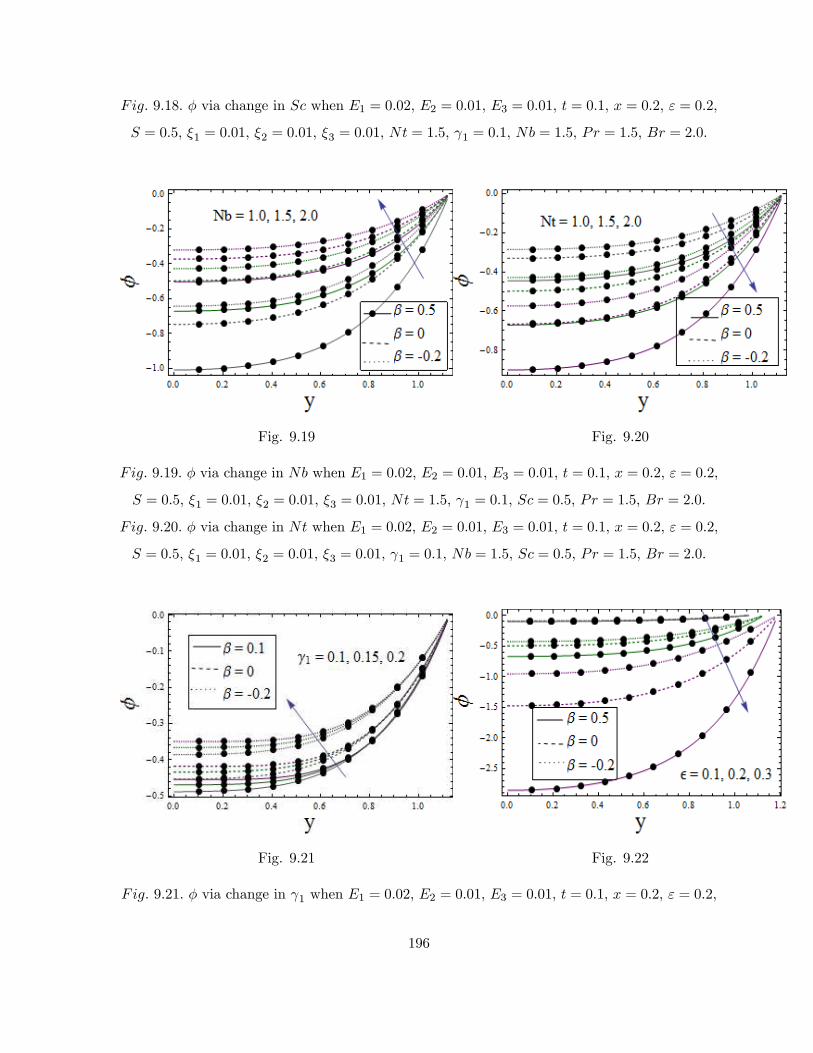
918 via change in when 1 = 002 2 = 001 3 = 001 = 01 = 02 = 02
= 05 1 = 001 2 = 001 3 = 001 = 15 1 = 01 = 15 = 15 = 20
Fig. 9.19 Fig. 9.20
919 via change in when 1 = 002 2 = 001 3 = 001 = 01 = 02 = 02
= 05 1 = 001 2 = 001 3 = 001 = 15 1 = 01 = 05 = 15 = 20
920 via change in when 1 = 002 2 = 001 3 = 001 = 01 = 02 = 02
= 05 1 = 001 2 = 001 3 = 001 1 = 01 = 15 = 05 = 15 = 20
Fig. 9.21 Fig. 9.22
921 via change in 1 when 1 = 002 2 = 001 3 = 001 = 01 = 02 = 02
196
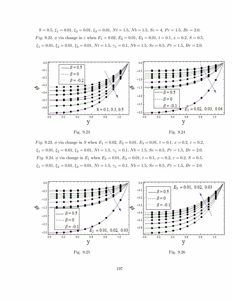
= 05 1 = 001 2 = 001 3 = 001 = 15 = 15 = 4 = 15 = 20
922 via change in when 1 = 002 2 = 001 3 = 001 = 01 = 02 = 05
1 = 001 2 = 001 3 = 001 = 15 1 = 01 = 15 = 05 = 15 = 20
Fig. 9.23 Fig. 9.24
923 via change in when 1 = 002 2 = 001 3 = 001 = 01 = 02 = 02
1 = 001 2 = 001 3 = 001 = 15 1 = 01 = 15 = 05 = 15 = 20
924 via change in 1 when 2 = 001 3 = 001 = 01 = 02 = 02 = 05
1 = 001 2 = 001 3 = 001 = 15 1 = 01 = 15 = 05 = 15 = 20
Fig. 9.25 Fig. 9.26
197

925 via change in 2 when 1 = 002 3 = 001 = 01 = 02 = 02 = 05
1 = 001 2 = 001 3 = 001 = 15 1 = 01 = 15 = 05 = 15 = 20
926 via change in 3 when 1 = 002 2 = 001 = 01 = 02 = 02 = 05
1 = 001 2 = 001 3 = 001 = 15 1 = 01 = 15 = 05 = 15 = 20
9.3.4 Entropy generation analysis
This subsection contains information about entropy analysis of the considered system for promi-
nent parameters of our study. Fig. 9.27 portrayed the effect of chemical reaction on . For
higher chemical reaction parameter the entropy enhances similar as in case of temperature.
Brinkman number also enhances the entropy as this parameter occurs due to the effect of vis-
cous dissipation which is responsible for enhancement of temperature and entropy (see Fig.
9.28). Fig. 9.29 witnessed increasing effect of heat source parameter. As expected the heat
source parameter enhances temperature and hence entropy. Influences of and Λ on are
opposite (see Figs. 9.30 and 9.31). Fig. 9.32 displays the impact of diffusion coefficient para-
meter Increasing trend of is noticed in this case. In all graphs it can be observed that
shear thinning fluids have higher entropy than the viscous and shear thickening materials. It is
due to the fact that shear thinning fluid has higher mean kinetic energy than shear thickening
materials which caused more disorderliness.
Fig. 9.27 Fig. 9.28
198
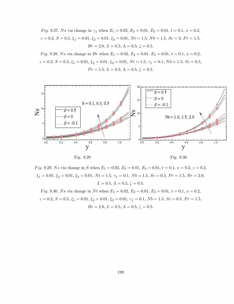
927 via change in 1 when 1 = 002 2 = 001 3 = 001 = 01 = 02
= 02 = 05 1 = 001 2 = 001 3 = 001 = 15 = 15 = 3 = 15
= 20 = 05 Λ = 05 = 05
928 via change in when 1 = 002 2 = 001 3 = 001 = 01 = 02
= 02 = 05 1 = 001 2 = 001 3 = 001 = 15 1 = 01 = 15 = 05
= 15 = 05 Λ = 05 = 05
Fig. 9.29 Fig. 9.30
929 via change in when 1 = 002 2 = 001 3 = 001 = 01 = 02 = 02
1 = 001 2 = 001 3 = 001 = 15 1 = 01 = 15 = 05 = 15 = 20
= 05 Λ = 05 = 05
930 via change in when 1 = 002 2 = 001 3 = 001 = 01 = 02
= 02 = 05 1 = 001 2 = 001 3 = 001 1 = 01 = 15 = 05 = 15
= 20 = 05 Λ = 05 = 05
199

Fig. 9.31 Fig. 9.32
931 via change in Λ when 1 = 002 2 = 001 3 = 001 = 01 = 02
= 02 = 05 1 = 001 2 = 001 3 = 001 = 15 1 = 01 = 15 = 05
= 15 = 20 = 05 = 05
932 via change in when 1 = 002 2 = 001 3 = 001 = 01 = 02
= 02 = 05 1 = 001 2 = 001 3 = 001 = 15 1 = 01 = 15 = 05
= 15 = 20 Λ = 05 = 05
9.3.5 Heat transfer coefficient
Graphs for heat transfer coefficient are displayed here for some influential parameters of our
study. These graphs are plotted for the shear thinning, viscous and shear thickening cases. It
can be seen that these graphs show oscillatory behavior which is due to peristaltic phenomenon.
Fig. 9.32 is arranged to see effect of chemical reaction. An increase is noticed here. Result
for on can be viewed from Fig. 9.33. Enhancement is observed. Fig. 9.34 displays
the increasing trend of for heat source. In all cases it can be clearly noticed that shear
thinning fluids have higher values for heat transfer coefficient than viscous and shear thickening
materials.
200

Fig. 9.33 Fig. 9.34
933 via change in 1 when 1 = 002 2 = 001 3 = 001 = 01 = 02 = 05
1 = 001 2 = 001 3 = 001 = 15 = 15 = 05 = 15 = 20
934 via change in when 1 = 002 2 = 001 3 = 001 = 01 = 02
= 05 1 = 001 2 = 001 3 = 001 = 15 1 = 01 = 15 = 05 = 15
Fig. 9.35
935 via change in when 1 = 002 2 = 001 3 = 001 = 01 = 02
1 = 001 2 = 001 3 = 001 = 15 1 = 01 = 15 = 05 = 15 = 20
201
9.4 Conclusions
Major findings are listed below.
• Velocity and thermal slip parameters lead to an increase in velocity and temperature.
• Velocity for shear thinning material is higher when compared with viscous and shearthickening fluids.
• Heat source parameter caused an increase in temperature and entropy.
• Temperature and entropy for shear thinning fluids are higher than viscous and shearthickening materials.
• Heat transfer coefficient enhances for chemical reaction parameter.
• Concentration for shear thickening fluids is higher than viscous and shear thinning mate-rials.
202
Chapter 10
Entropy analysis in peristalsis with
homogeneous-heterogeneous reaction
10.1 Introduction
Homogeneous-heterogeneous reactions in peristalsis of Prandtl fluid are examined. Magnetic
field is applied in the perpendicular direction to the flow. Joule heating effect is also considered
in this analysis. Buongiorno nanofluid model has been used which incorporates two prominent
slip mechanisms i.e. Brownian motion and thermophoresis. Second law of thermodynamics has
been utilized for entropy generation analysis. No slip boundary conditions are employed for
the considered analysis. NDSolve command of Mathematica 9.0 is employed for the solution of
problem. Graphs for pertinent parameters are plotted and analyzed. These graphs contain ve-
locity, temperature, homogeneous-heterogeneous reaction, entropy and heat transfer coefficient.
Key points are summarized in the conclusion.
10.2 Problem formulation
MHD peristaltic flow of the incompressible Prandtl nanofluid is considered. Peristaltic wave
travel along the flexible walls of channel. Wall’s temperature are maintained at 1 and 0 and
concentration 1 and 0 respectively (see Fig. 10.1). Homogeneous- heterogeneous reaction is
considered for the considered problem. Nanofluid slip mechanisms, Brownian motion and ther-
203

mophoresis are considered. Joule heating and viscous dissipation are also accounted. Peristaltic
wave shape is
= ± ( ) = ±∙+ sin
2
(− )
¸ (10.1)
Here wall shape is denoted by ± with and denote the half channel width, wave
amplitude, time and wave speed.
Fig. 10.1: Flow configuration
The model equations for homogeneous-heterogeneous equations are
+ 2 → 3 rate ∗1
2∗2 (10.2)
in which and elucidate the rate constants. We consider the single first order isothermal
reaction. On the surface of catalyst we have
→ rate ∗1 (10.3)
where ∗1 ∗2 are the respective concentration of the species and Flow expressions are
+
= 0 (10.4)
+
+
= − 1
+1
+1
− 1
20 (10.5)
204

+
+
= − 1
+1
+1
(10.6)
+
+
= ∗
∙2
2+
2
2
¸+
1
()
∙
+
µ
+
¶+
¸
+
⎡⎢⎣
³∗1
+
∗1
+
∗2
+
∗2
´+
µ¡
¢2+³
´2¶⎤⎥⎦
+1
()20
2 (10.7)
∗1
+ ∗1
+ ∗1
=
µ2∗12
+2∗12
¶−
∗1
2∗2 +
∙2
2+
2
2
¸ (10.8)
∗2
+ ∗2
+ ∗2
=
µ2∗22
+2∗22
¶+
∗1
2∗2 +
∙2
2+
2
2
¸ (10.9)
Here describe respective velocity components and temperature. the pressure,
density, the stress components of the considered Prandtl fluid. ∗ the thermal
diffusivity, (= () () ) the ratio of specific heat capacity of nanoparticles and base
fluid, the Brownian motion and the thermophoretic diffusion coefficients, the mean
temperature of the fluid, and and the diffusion species coefficients for the species and
respectively.
Prandtl fluid can be expressed by the following relation:
τ = −I+ S (10.10)
where the component is given by
=
∗ arcsin
Ã1∗
∙³
´2+¡
¢2¸ 12!∙³
´2+¡
¢2¸ 12
(10.11)
With the boundary conditions
= 0 at = ± (10.12)
205

=
⎧⎨⎩ 1
0
⎫⎬⎭ at = ± (10.13)
∗1−
∗1 = 0 at = ∗1 → 0 at = − (10.14)
∗2
+ ∗2 = 0 at = ∗2 → 0 at = − (10.15)
The equation mentioned below describe the decomposition of applied pressure in terms of
compliant walls characteristics.
∙−∗
3
3+∗
3
2+ ∗1
2
¸ =
+
−
∙
+
+
¸−20 at = ± (10.16)
Non-dimensional parameters are
∗ =
∗ =
∗ =
∗ =
∗ =
∗ =
=
− 0
1 − 0 ∗ =
=
∗10
=∗20
∗ =2
=
= −
(10.17)
After utilizing non-dimensional parameters, we obtained the following systems
Re
∙2
+
2
−
2
2
¸= −
+
+
−2
(10.18)
Re
∙−2
2
− 2
2
2+ 2
2
¸= −
+ 2
+
(10.19)
206

RePr
∙
+
−
¸=
∙22
2+
2
2
¸+
∙
2
+
µ2
2− 2
2
2
¶−
2
¸+Pr
µ2
+
+ 2
+
¶+Pr
Ã2µ
¶2+
µ
¶2!+2
µ
¶2(10.20)
Re
∙
+
−
¸=
1
∙22
2+
2
2
¸−2 +
1
∙22
2+
2
2
¸
(10.21)
Re
∙
+
−
¸=
∗
∙22
2+
2
2
¸+2 +
1
∙22
2+
2
2
¸
(10.22)
= 12
2+
6
"µ2
2
¶2+ 4
µ2
2
¶2#µ2
2
¶ (10.23)
= 0, at = ± = ±(1 + sin 2 (− )) (10.24)
∙1
3
3+2
3
2+3
2
¸ = −Re
∙2
+
2
−
2
2
¸+
+
−2
at = ± (10.25)
=
⎧⎨⎩ 1
0
⎫⎬⎭ at = ± (10.26)
− = 0 at = = 1 at = − (10.27)
∗
+ = 0 at = = 0 at = − (10.28)
207

with
Re =
=
=
r
0 =
= (1 − 0)
=
0
=
Pr = ()
=
2
(1 − 0) 1 =
∗
∗
=1
2
∗22
=
=
=
202
1 = − ∗3
3 2 =
∗3
3 3 =
∗13
2 (10.29)
where Re depicts Reynolds number, wave number, Hartman number, amplitude ratio,
thermophoresis parameter, Brownian motion parameter, Schmidt number, Pr Prandtl
number, Brinkman number, 1 and are fluid parameters for Prandtl fluid, Diffusion
Schmidt number, and measures the strength of respective heterogeneous and homogeneous
reactions and 1 2 3 the compliant walls coefficients. Here we have omitted the asterisks
for simplicity.
After employing the theory of long wavelength and low Reynolds number assumptions we
obtain
=
−2
(10.30)
= 0 (10.31)
2
2+
∙
2
2
¸+Pr
µ
+
¶+Pr
µ
¶2+2
µ
¶2= 0 (10.32)
1
2
2−2 +
1
2
2= 0 (10.33)
∗
2
2+2 +
1
2
2= 0 (10.34)
208

= 12
2+
6
µ2
2
¶3 (10.35)
= 0, at = ± = ±(1 + sin 2 (− )) (10.36)
∙1
3
3+2
3
2+3
2
¸ =
−2
at = ± (10.37)
=
⎧⎨⎩ 1
0
⎫⎬⎭ at = ± (10.38)
− = 0 at = = 1 at = − (10.39)
∗
+ = 0 at = = 0 at = − (10.40)
In general the diffusion coefficient of the chemical species and are of comparable size. For
application point of view this leads to the assumption that they are equal i.e. = and
hence ∗ =
= 1 and we have the relation + = 1 After utilizing this relation, We solved
these equations via NDSolve of Mathematica.
10.2.1 Entropy generation
Entropy expression obeys
000 =
2
õ
¶2+
µ
¶2!+
202
+Φ
+
õ∗1
¶2+
µ∗1
¶2!+
µ∗1
+
∗1
¶+
+
õ∗2
¶2+
µ∗2
¶2!+
µ∗2
+
∗2
¶ (10.41)
where Φ is given by
Φ =
+
+
µ
+
¶ (10.42)
209

Dimensionless form satisfies
=000
000
=
µ
¶2+
2
Λ
µ
¶2+
Λ
µ2
2
¶+1
Λ
µ
¶µ
¶+
1
Λ2
µ
¶2+
+2
Λ
µ
¶µ
¶+
2
Λ2
µ
¶2 (10.43)
000 =
(1 − 0)2
22
Λ =1 − 0
1 =
0
2 =
0
=
0
(10.44)
10.3 Analysis
Here we adopted the technique (NDSolve command of Mathematica) which gave the convergent
solution in less computation time. Moreover this technique avoids the lengthy complicated
expressions. Graphs are plotted directly for the physical analysis. These graphs include velocity,
temperature, entropy and heat transfer coefficient. Figs. 10.2 and 10.3 displayed the results
for fluid parameter on velocity. Decay in both cases is observed. Same results can be seen via
studies [84, 85]. Magnetic field effect (utilized in ECG for synchronization purposes) can be
observed via Fig. 10.4. As Lorentz force caused resistance in fluid flow. So decrease in fluid
velocity has been observed. Fig. 10.5 manifested the effect of wall parameters. Decrease is
noticed via damping nature of walls whereas an increase in velocity is observed for elastance
characteristics of walls. These results have quite resemblance with the flow in blood vessels
where the elastance nature enhances the blood velocity and damping nature reduced the blood
velocity.
210

Fig. 10.2 Fig. 10.3
102 for 1 when 1 = 002 2 = 001 3 = 001 = 01 = 02 = 02 = 05
= 01 = 05 = 05 = = 05 = 01 = 01 = 15 = 20
103 for when 1 = 002 2 = 001 3 = 001 = 01 = 02 = 02 1 = 20
= 01 = 05 = 05 = = 05 = 01 = 01 = 15 = 20
Fig. 10.4 Fig. 10.5
104 for when 1 = 002 2 = 001 3 = 001 = 01 = 02 = 02 1 = 20
= 05 = 05 = 05 = = 05 = 01 = 01 = 15 = 20
105 for 1 2 and 3 when = 01 = 02 = 02 1 = 20 = 05 = 01
211

= 05 = 05 = = 05 = 01 = 01 = 15 = 20
Temperature profile for effect of fluid parameters ( ) can be viewed through Figs. 10.6
and 10.7. Decrease is noticed in these cases as can be seen through studies [84, 85]. As
enhancement in mean kinetic energy of the particles leads to increase in temperature. Here
higher values of fluid parameters slow down the fluid velocity so particles have less molecular
vibrations and thus less temperature as well. Influence of Brinkman number on is notified via
Fig. 10.8. Note that resistance among fluid particle due to viscous effects produced heat. It
results in enhancement of temperature of fluid. Fig. 10.9 elucidates the magnetic field influence
on Applied magnetic field provide resistance to fluid which produce heating and caused an
increase in temperature. Figs. 10.10 and 10.11 are manifested for the behaviors of and
on temperature. Larger values for both parameters caused an increase in temperature of fluid.
is related to random motion of the particles. Larger values of it indicate more randomness
and hence more heat loss which leads to increase in temperature. Fig. 10.12 displays the
results for homogeneous reaction parameter on temperature. Decrease in seen in this case. As
concentration deceases in this case so less concentrated fluid have less heat loss. Compliant wall
characteristics are seen qualitatively similar with (see Fig. 10.13). Compliant characteristics
of walls are important as when wall are elastic it easily allows the exchange of water, oxygen
and other nutrients.
Fig. 10.6 Fig. 10.7
212

106 for 1 when 1 = 002 2 = 001 3 = 001 = 01 = 02 = 02 = 05
= 01 = 05 = 05 = = 05 = 01 = 01 = 15 = 20
107 for when 1 = 002 2 = 001 3 = 001 = 01 = 02 = 02 1 = 20
= 01 = 05 = 05 = = 05 = 01 = 01 = 15 = 20
Fig. 10.8 Fig. 10.9
108 for when 1 = 002 2 = 001 3 = 001 = 01 = 02 = 02 1 = 20
= 05 = 01 = 05 = 05 = = 05 = 01 = 01 = 15
109 for when 1 = 002 2 = 001 3 = 001 = 01 = 02 = 02 1 = 20
= 05 = 05 = 05 = = 05 = 01 = 01 = 15 = 20
213

Fig. 10.10 Fig. 10.11
1010 for when 1 = 002 2 = 001 3 = 001 = 01 = 02 = 02
1 = 20 = 05 = 01 = 05 = 05 = = 05 = 01 = 15 = 20
1011 for when 1 = 002 2 = 001 3 = 001 = 01 = 02 = 02 1 = 20
= 05 = 01 = 05 = 05 = = 05 = 01 = 15 = 20
Fig. 10.12 Fig. 10.13
1012 for when 1 = 002 2 = 001 3 = 001 = 01 = 02 = 02 1 = 20
= 05 = 01 = 05 = 01 = = 05 = 01 = 15 = 20
1013 for 1 2 3 when = 01 = 02 = 02 1 = 20 = 05 = 01
214

= 05 = 05 = = 05 = 01 = 01 = 15 = 20
Figs. 10.14 and 10.15 are plotted to observe the effect of heterogeneous and homogeneous
reaction parameters on Decaying behavior of these parameters on concentration has been
noticed. As increase in heterogeneous reaction parameter enhances the reaction rate which
results in decrease of diffusion rate and hence concentration decreases whereas enhancement
in homogeneous reaction parameter caused reduction in viscosity and hence in concentration.
Fig. 10.16 is prepared for (Hartman number) effect on concentration. Enhancement in
concentration is seen here. Larger values of Schmidt number caused decay in concentration (see
Fig. 10.17). As density of the fluid decreases. So less dense particles attained higher speed and
it lessons the fluid concentration.
Fig. 10.14 Fig. 10.15
1014 for when 1 = 002 2 = 001 3 = 001 = 01 = 02 = 02 1 = 20
= 05 = 01 = 05 = = 05 = 01 = 01 = 15 = 20
1015 for when 1 = 002 2 = 001 3 = 001 = 01 = 02 = 02 1 = 20
= 05 = 01 = 05 = = 05 = 01 = 01 = 15 = 20
215

Fig. 10.16 Fig. 10.17
1016 for when 1 = 002 2 = 001 3 = 001 = 01 = 02 = 02 1 = 20
= 05 = 05 = 05 = = 05 = 01 = 01 = 15 = 20
1017 for when 1 = 002 2 = 001 3 = 001 = 01 = 02 = 02
1 = 20 = 05 = 01 = 05 = 05 = 01 = 01 = 15 = 20
Entropy analysis for different embedded parameters has been carried out through Figs.
10.18—10.30. Hartman number impact can be observed via Fig. 10.18. As magnetic field provide
resistance that produced heating so temperature enhances at the center of channel. Fig. 10.19
portrayed the results for on Random motion of particles create more disorderedness
hence entropy enhances for higher Similar behavior has been seen for via Fig. 10.20.
Entropy for Schmidt number is decreased (see Fig. 10.21). As less concentrated fluid has
no more disorderedness. Fig. 10.22 demonstrated that increase in heterogeneous reaction
caused enhancement in entropy generation. 1 and 2 results are displayed via Fig. 10.23.
Enhancement is observed here. Fig. 10.24 is prepared for the study of Brinkman number
impact on entropy. Obviously increase is noticed in this case. As increase in viscous dissipation
produces more heating and thus increase in entropy. Opposite impacts for and Λ have
been observed (see Figs. 10.25 and 10.26). Fluid parameters for Prandtl number results are
illustrated via Figs. 10.27 and 10.28. Decrease is noticed like in the case of temperature.
Entropy analysis for homogeneous reaction parameter can be observed through Fig. 10.29.
216

Decay is observed through reason directly linked to temperature. Compliant wall results are
seen increasing for elastance coefficients whereas decreasing for damping coefficient (see Fig.
10.30).
Fig. 10.18 Fig. 10.19
1018 for when 1 = 002 2 = 001 3 = 001 = 01 = 02 = 02
1 = 02 = 05 = 05 = 05 = = 01 = 01 = 01 = 15
= 20 Λ = 05 = 05 1 = 2 = 05
1019 for when 1 = 002 2 = 001 3 = 001 = 01 = 02 = 02
1 = 20 = 05 = 01 = 05 = 05 = = 05 = 01 = 15 = 20
Λ = 05 = 05 1 = 2 = 05
217

Fig. 10.20 Fig. 10.21
1020 for when 1 = 002 2 = 001 3 = 001 = 01 = 02 = 02
1 = 20 = 05 = 01 = 05 = 05 = = 05 = 01 = 01 = 15
= 20 Λ = 05 = 05 1 = 2 = 05
1021 for when 1 = 002 2 = 001 3 = 001 = 01 = 02 = 02
1 = 20 = 05 = 01 = 05 = 05 = 01 = 01 = 15 = 20
Λ = 05 = 05 1 = 2 = 05
Fig. 10.22 Fig. 10.23
1022 for when 1 = 002 2 = 001 3 = 001 = 01 = 02 = 02
218

1 = 20 = 05 = 01 = 05 = = 05 = 01 = 01 = 15
= 20 Λ = 05 = 05 1 = 2 = 05
1023 for 1 2 when 1 = 002 2 = 001 3 = 001 = 01 = 02 = 02
1 = 20 = 05 = 01 = 05 = 05 = = 05 = 01 = 01 = 15
= 20 Λ = 05 = 05
Fig. 10.24 Fig. 10.25
1024 for when 1 = 002 2 = 001 3 = 001 = 01 = 02 = 02
1 = 20 = 05 = 01 = 05 = 05 = = 05 = 01 = 01 = 15
Λ = 05 = 05 1 = 2 = 05
1025 for when 1 = 002 2 = 001 3 = 001 = 01 = 02 = 02
1 = 20 = 05 = 01 = 05 = 05 = = 05 = 01 = 01 = 15
219

= 20 Λ = 05 1 = 2 = 05
Fig. 10.26 Fig. 10.27
1026 for Λ when 1 = 002 2 = 001 3 = 001 = 01 = 02 = 02
1 = 20 = 05 = 01 = 05 = 05 = = 05 = 01 = 01 = 15
= 20 = 05 1 = 2 = 05
1027 for 1 when 1 = 002 2 = 001 3 = 001 = 01 = 02 = 02
= 05 = 01 = 05 = 05 = = 05 = 01 = 01 = 15
= 20 Λ = 05 = 05 1 = 2 = 05
Fig. 10.28 Fig. 10.29
1028 for when 1 = 002 2 = 001 3 = 001 = 01 = 02 = 02
220

1 = 20 = 01 = 05 = 05 = = 05 = 01 = 01 = 15
= 20 Λ = 05 = 05 1 = 2 = 05
1029 for when 1 = 002 2 = 001 3 = 001 = 01 = 02 = 02
1 = 20 = 01 = 05 = 05 = = 05 = 01 = 01 = 15
= 20 Λ = 05 = 05 1 = 2 = 05
Fig. 10.30
1030 for 1 2 3 when = 01 = 02 = 02 1 = 20 = 05 = 01
= 05 = 05 = = 05 = 01 = 01 = 15 = 20 Λ = 05 = 05
1 = 2 = 05
Figs. 10.31-10.34 are plotted for investigation of heat transfer coefficient under influence
of pertinent parameters. Fluid parameter for Prandtl fluid results can be discussed via Figs.
10.31 and 10.32. Increasing trend of is noticed for both parameters. Brinkman number effect
can be seen through Fig. 10.33. Larger values of increases the heat transfer coefficient.
Hartman number effect can be portrayed via Fig. 10.34. Decay in heat transfer coefficient is
noticed for higher
221
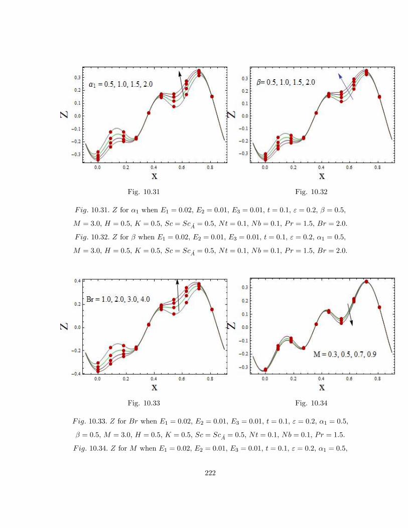
Fig. 10.31 Fig. 10.32
1031 for 1 when 1 = 002 2 = 001 3 = 001 = 01 = 02 = 05
= 30 = 05 = 05 = = 05 = 01 = 01 = 15 = 20
1032 for when 1 = 002 2 = 001 3 = 001 = 01 = 02 1 = 05
= 30 = 05 = 05 = = 05 = 01 = 01 = 15 = 20
Fig. 10.33 Fig. 10.34
1033 for when 1 = 002 2 = 001 3 = 001 = 01 = 02 1 = 05
= 05 = 30 = 05 = 05 = = 05 = 01 = 01 = 15
1034 for when 1 = 002 2 = 001 3 = 001 = 01 = 02 1 = 05
222

= 05 = 05 = 05 = = 05 = 01 = 01 = 15 = 20
10.3.1 Validation of problem:
To validate the results of our problem we have compared the results with study by Alsaedi et
al [80]. They have utilized the perturbation method to solve their problem. We have made a
comparison about velocity profile. In our problem if we exclude the nanofluid and homogeneous-
heterogeneous reaction then our results are in good comparison with the study [80].
Fig. 10.35: Validation of the Problem
1035 for when 1 = 1 2 = 05 3 = 05 = 01 = 03 = 02 1 = 10
= 01 = 0 = 0 = 0 = 15 = 20
10.4 Conclusions
This study discloses the phenomenon of peristalsis with homogeneous-heterogeneous reaction.
Entropy analysis has been carried out. Some important observations for the considered analysis
can be summed up as follows:
• Prandtl number has decaying behavior for velocity, temperature and entropy generation.
• Magnetic field slows down the fluid velocity whereas it provides heating to the fluid andincrease the system’s entropy.
223

• Heterogeneous reaction parameter enhances the entropy.
• Temperature increases for and Qualitatively similar behavior is observed for
entropy.
• Homogeneous reaction parameter has same result on temperature and entropy.
• Concentration decreases for homogeneous and heterogeneous reaction parameters.
• Heat transfer coefficient rises for fluid parameter and Brinkman number whereas it de-creases for Hartman number.
224

Chapter 11
Entropy analysis for the peristaltic
flow of third grade fluid with
variable thermal conductivity
11.1 Introduction
This chapter is based on the study of entropy analysis in fluid transport phenomenon by peri-
stalsis. Mixed convective flow in compliant wall channel is considered. Here third grade fluid
is considered. Effect of gravity is also encountered. Magnetohydrodynamics and Joule heating
are part of flow modeling. Energy equation is addressed subject to viscous dissipation and
variable thermal conductivity. Resulting system is solved with the help of NDSolve command
in Mathematica. Proper attention is given to the study of velocity, temperature and entropy
analysis. This analysis is carried out via graphical results for different embedded parameters.
Graphs for heat transfer coefficient are also plotted and analyzed.
11.2 Modeling
Here we modeled the peristaltic phenomenon of an incompressible third grade fluid. The channel
is considered vertical. Here x-axis lies along the flow direction and y-axis perpendicular to it
(see Fig. 11.1). As the channel is vertical so effects of gravity cannot be ignored. Thus mixed
225

convection is also taken into account in this study. The channel walls are flexible. MHD and
Joule heating phenomena are accounted. Here peristaltic waves are propagating in x-direction.
Wave amplitude is with speed wavelength and channel width 2 Temperature of the left
wall is maintained at 0 and right wall by 1 Shape of wall is given by:
= ± ( ) = ±∙+ sin
2
(− )
¸ (11.1)
Fig. 11.1: Flow Diagram
An extra stress tensor for thermodynamic compatible third grade fluid is [79]
S = A1 + 1A2 + 2A21 + (A21)A1 (11.2)
in which material parameters satisfy the conditions
1 ≥ 0 ≥ 0 |1 + 2| ≤p24 (11.3)
The definitions of first and second Rivilin-Ericksen tensors are [79]
A1 = ∇V+(∇V) A2 =A1
+A1(∇V) + (∇V) A1 (11.4)
where material derivative is given by (
+
+
)
226

Flow configuration is described by the following set of equations [100, 181]
Continuity equation is:
+
= 0 (11.5)
Momentum equation in presence of MHD and mixed convection satisfies
µ
+
+
¶= −
+
+
− 20+ ( − 0) (11.6)
µ
+
+
¶= −
+
+
(11.7)
Energy expression in presence of variable thermal conductivity, Joule heating and viscous dis-
sipation leads to
µ
+
+
¶=
µ( )
¶+
µ( )
¶+
+
µ
+
¶+
+202 (11.8)
The boundary conditions are stated as follows
= 0 at = ± (11.9)
=
⎧⎨⎩ 1
0
⎫⎬⎭ at = ± (11.10)
∙−∗
3
3+∗
3
2+ ∗1
2
¸ =
+
−
∙
+
+
¸−20+ ( − 0) at = ±(11.11)
Here and are the velocity components in the and directions, the pressure, ( ) the
variable thermal conductivity, the density, the specific heat, 0 the strength of magnetic
field, the electric conductivity, the components of third grade fluid, the gravity,
the thermal expansion coefficient, for temperature and ∗ ∗ and ∗1 the compliant walls
coefficients that describes the elastic and damping characteristics of the walls.
227

Non-dimensional quantities are
∗ =
∗ =
∗ =
∗ =
∗ =
∗ =
() =
( )
0 ∗ =
∗ =
2
∗ =2
2 =
− 0
1 − 0 =
= −
(11.12)
Utilizing (11.12) one has in terms of stream function () as
Re
∙2
+
2
−
2
2
¸= −
+
+
−2
+ (11.13)
Re
∙−2
2
− 2
2
2+ 2
2
¸= −
+ 2
+
(11.14)
RePr
∙
+
−
¸= 2
µ()
¶+
µ()
¶+
+
∙
2
+
µ2
2− 2
2
2
¶−
2
¸+2
µ
¶2 (11.15)
= 0, at = ± = ±(1 + sin 2 (− )) (11.16)
∙1
3
3+2
3
2+3
2
¸ = −Re
∙2
+
2
−
2
2
¸+
+
−2
+ at = ±(11.17)
=
⎧⎨⎩ 1
0
⎫⎬⎭ at = ± (11.18)
228
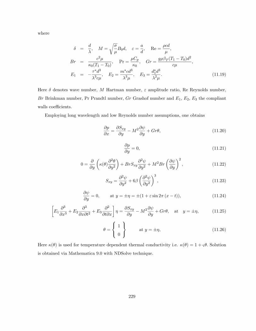
where
=
=
r
0 =
Re =
=2
0(1 − 0) Pr =
0 =
(1 − 0)2
1 = − ∗3
3 2 =
∗3
3 3 =
∗13
2 (11.19)
Here denotes wave number, Hartman number, amplitude ratio, Re Reynolds number,
Brinkman number, Pr Prandtl number, Grashof number and 1 2 3 the compliant
walls coefficients.
Employing long wavelength and low Reynolds number assumptions, one obtains
=
−2
+ (11.20)
= 0 (11.21)
0 =
µ()
2
2
¶+
2
2+2
µ
¶2 (11.22)
=2
2+ 6
µ2
2
¶3 (11.23)
= 0, at = ± = ±(1 + sin 2 (− )) (11.24)
∙1
3
3+2
3
2+3
2
¸ =
−2
+ at = ± (11.25)
=
⎧⎨⎩ 1
0
⎫⎬⎭ at = ± (11.26)
Here () is used for temperature dependent thermal conductivity i.e. () = 1 + Solution
is obtained via Mathematica 9.0 with NDSolve technique.
229

11.2.1 Entropy generation
Mathematical expression for entropy analysis is [214]:
000 =
( )
2
õ
¶2+
µ
¶2!| z
+20
2
| z
+Φ
|z
(11.27)
where Φ is given by
Φ =
+
+
µ
+
¶ (11.28)
In dimensionless form
=000
000
= ()
µ
¶2+
2
Λ
µ
¶2+
Λ
µ2
2
¶ (11.29)
000 =
0 (1 − 0)2
22
Λ =1 − 0
(11.30)
11.3 Analysis
Here NDSolve of Mathematica is used for the solution of nonlinear system. Graphical results
with physical interpretations are arranged in the separate subsections for simplicity.
11.3.1 Velocity
This subsection contains the information about velocity. Results of some physical parameters
including , , , , and 1 2 3 are examined. Grashof number behavior can be
portrayed via Fig. 11.2. The buoyancy forces facilitate the flow. An increase is noticed clearly
in this case. Opposite result for Hartman number is noticed via Fig. 11.3. As the resistive
nature forces caused reduction in flow. Here Lorentz force plays this role. Applied magnetic
field provides resistance to fluid particles. This fact is utilized for reduction of bleeding during
surgeries and cancer tumor treatment. Influence of variable thermal conductivity parameter is
seen via Fig. 11.4. Increase in caused an enhancement of velocity. Fig. 11.5 is prepared for
fluid parameter result. Fluid parameter leads to an increase of velocity. It is because of decrease
in viscosity parameter. Here leads to an enhancement in fluid velocity (see Fig. 11.6). Same
230

results can be seen through study [79] for the cases of and Obviously as increase in wave
amplitude caused an enhancement of fluid velocity. Flexible characteristics of walls impacts
can be viewed via Fig. 11.7. Elastance parameters facilitate the flow whereas damping leads to
slow down the fluid particles. These characteristics of walls have association with blood vessels.
Fig. 11.2 Fig. 11.3
112 versus when 1 = 002 2 = 001 3 = 001 = 01 = 02 = 02
= 001 = 001 = 10 = 20
113 versus when 1 = 002 2 = 001 3 = 001 = 01 = 02 = 02
= 001 = 001 = 01 = 20
231

Fig. 11.4 Fig. 11.5
114 versus when 1 = 002 2 = 001 3 = 001 = 01 = 02 = 02
= 001 = 01 = 10 = 20
115 versus when 1 = 002 2 = 001 3 = 001 = 01 = 02 = 02
= 001 = 01 = 10 = 20
Fig. 11.6 Fig. 11.7
116 versus when 1 = 002 2 = 001 3 = 001 = 01 = 02 = 001
= 001 = 01 = 10 = 20
117 versus 1 2 and 3 when = 01 = 02 = 02 = 001 = 001
232

= 01 = 10 = 20
11.3.2 Temperature
This subsection contains information about temperature for different embedded parameters.
Grashof number results can be seen via Fig. 11.8. Temperature is known as average kinetic
energy. Thus an increase in the mean kinetic energy of the particles caused higher fluid tem-
perature. Fluid parameter () leads to decrease of temperature (see Fig. 11.9). As increase in
fluid parameter decreases the viscosity. There is less heat loss and temperature decays. Study
[79] reports the same observation. Hartman number caused an increase in temperature of fluid
near the center of channel. It is due to Joule heating (see Fig. 11.10). Behavior for variable
thermal conductivity parameter has been seen via Fig. 11.11. An increase in temperature
is observed for this case. As increase in enhances the conductance property of fluid which
increases temperature as well. Same result for variable thermal conductivity parameter has
been examined in study [77]. Fig. 11.12 elucidated the behavior of on Larger values of
amplitude lead to an enhancement of temperature. This is also caused by an increase of mean
kinetic energy of particles. Fig. 11.13 portrayed impact on Clearly an increase is viewed
through view of viscous dissipation. Fig. 11.14 displays the results of flexible characteristics of
walls. Here 1, 2 results are opposite to that of 3
Fig. 11.8 Fig. 11.9
233

118 versus when 1 = 002 2 = 001 3 = 001 = 01 = 02 = 02
= 001 = 001 = 10 = 20
119 versus when 1 = 002 2 = 001 3 = 001 = 01 = 02 = 02
= 001 = 01 = 10 = 20
Fig. 11.10 Fig. 11.11
1110 versus when 1 = 002 2 = 001 3 = 001 = 01 = 02 = 02
= 001 = 001 = 01 = 20
1111 versus when 1 = 002 2 = 001 3 = 001 = 01 = 02 = 02
= 001 = 01 = 10 = 20
234
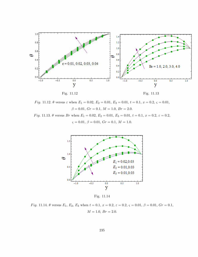
Fig. 11.12 Fig. 11.13
1112 versus when 1 = 002 2 = 001 3 = 001 = 01 = 02 = 001
= 001 = 01 = 10 = 20
1113 versus when 1 = 002 2 = 001 3 = 001 = 01 = 02 = 02
= 001 = 001 = 01 = 10
Fig. 11.14
1114 versus 1 2 3 when = 01 = 02 = 02 = 001 = 001 = 01
= 10 = 20
235

11.3.3 Entropy analysis
This subsection covers the entropy analysis for the considered system. Graphs for embedded
parameters provide the information about entropy () of the system. Figs. 11.15-11.22 are
plotted for this purpose. Grashof number impact can be viewed via Fig. 11.15. It can be
seen that high temperature also leads to an increase of system’s entropy. Clearly Joule heating
phenomenon rises the temperature of fluid and thus entropy enhances (see Fig. 11.16). Fig.
11.17 describes the effect of Λ on Larger values of Λ caused decay in Fluid parameter
results can be observed with the help of Fig. 11.18. Clearly increasing values of tend to
decrease the entropy of system. Such fact can be verified by relating it with temperature.
Fig. 11.19 is prepared to study effect of on temperature. An enhancement in is noticed
clearly. Variable thermal conductivity parameter impact can be elucidated via Fig. 11.20. The
results are seen qualitatively similar to that of temperature. Larger values of Brinkman number
enhance the entropy of system (see Fig. 11.21). As more viscous dissipation lead to increase of
temperature and hence more disorderliness. Walls parameters behavior has quite resemblance
with temperature (see Fig. 11.22).
Fig. 11.15 Fig. 11.16
1115 versus when 1 = 002 2 = 001 3 = 001 = 01 = 02 = 02
= 001 = 001 = 10 = 20 Λ = 05
1116 versus when 1 = 002 2 = 001 3 = 001 = 01 = 02 = 02
236

= 001 = 001 = 01 = 20 Λ = 05
Fig. 11.17 Fig. 11.18
1117 versus Λ when 1 = 002 2 = 001 3 = 001 = 01 = 02 = 02
= 001 = 001 = 01 = 10 = 20
1118 versus when 1 = 002 2 = 001 3 = 001 = 01 = 02 = 02
= 001 = 01 = 10 = 20 Λ = 05
Fig. 11.19 Fig. 11.20
1119 versus when 1 = 002 2 = 001 3 = 001 = 01 = 02 = 001
= 001 = 01 = 10 = 20 Λ = 05
237

1120 versus when 1 = 002 2 = 001 3 = 001 = 01 = 02 = 02
= 001 = 01 = 10 = 20 Λ = 05
Fig. 11.21 Fig. 11.22
1121 versus when 1 = 002 2 = 001 3 = 001 = 01 = 02 = 02
= 001 = 001 = 01 = 10 Λ = 05
1122 versus 1 2 and 3 when = 01 = 02 = 02 = 001 = 001
= 01 = 10 = 20 Λ = 05
11.3.4 Heat transfer coefficient
This subsection is devoted to the results for heat transfer coefficient. Fig. 11.23 portrayed
the effect of on Grashof number is an increasing function of heat transfer coefficient.
Opposite behavior of Hartman number on heat transfer coefficient is observed (see Fig. 11.24).
Figs. 11.25 and 11.26 display the influences of and on heat transfer coefficient () Both
parameters depict similar impact on Fig. 11.27 represents the influence on Heat
transfer coefficient increases for These observations for and are similar to that as in
ref. [79]. ( = 1 2) show increasing trend and 3 illustrate decreasing effect of (see Fig.
11.28).
238

Fig. 11.23 Fig. 11.24
1123 versus when 1 = 002 2 = 001 3 = 001 = 01 = 02 = 001
= 001 = 20 = 10
1124 versus when 1 = 002 2 = 001 3 = 001 = 01 = 02 = 001
= 001 = 01 = 20
Fig. 11.25 Fig. 11.26
1125 versus when 1 = 002 2 = 001 3 = 001 = 01 = 02 = 001
= 01 = 10 = 20
1126 versus when 1 = 002 2 = 001 3 = 001 = 01 = 02 = 001
= 01 = 10 = 20
239

Fig. 11.27 Fig. 11.28
1127 versus when 1 = 002 2 = 001 3 = 001 = 01 = 02 = 001
= 001 = 01 = 10
1128 versus 1 2 3 when = 01 = 02 = 001 = 001 = 01 = 10
= 20
11.3.5 Trapping
Trapping is discussed in this subsection for some prominent parameters. Decrease is noticed
for the size of trapped bolus for larger Hartman number (see Fig. 11.29 (a) and (b)).
impact on bolus size can be noticed via Fig. 11.30 (a) and (b). Bolus size increases in this
case. Fig. 11.31 (a) and (b) displayed that bolus size decreases for the case of variable thermal
conductivity parameter.
240

Fig. 11.29 (a) (b)
1129 versus when 1 = 002 2 = 001 3 = 001 = 00 = 02 = 001
= 001 = 20 () = 10 () = 15
Fig. 11.30 (a) (b)
1130 versus when 1 = 002 2 = 001 3 = 001 = 00 = 02 = 001
= 001 = 10 = 20 () = 01 () = 05
241

Fig. 11.31 (a) (b)
1131 versus when 1 = 002 2 = 001 3 = 001 = 00 = 02 = 001
= 10 = 20 () = 01 () = 03
11.4 Conclusions
Important points of present study can be summarized as follows:
• Variable thermal conductivity parameter increases the velocity, temperature and entropyof system.
• Hartman number caused decay in velocity but it increases the entropy and temperaturenear the center of channel.
• effect on temperature, entropy and heat transfer coefficient are same.
• Bolus size decreases for
242

Bibliography
[1] W. M. Bayliss and E. H. Starling, The movement and innervation of the small intestine,
J. Physiol., 24 (1899) 99-143.
[2] T. W. Engelmann, Zur Physiologie des Ureter, Pflug. Arch. Ges. Physiol., 2 (1869) 243-
293.
[3] J. Lapides, The physiology of the intact human ureter., J. Urol., 59 (1948) 501-537.
[4] S. Boyarsky, Surgical physiology of the renal pelvis and ureter, Monogr. Sur. Sci., 1 (1964)
173-213.
[5] T. W. Latham, Fluid motion in a peristaltic pump, M.S. Thesis, MIT., Cambridge, MA
(1966).
[6] A. H. Shapiro, M. Y. Jafrin and S. L. Weinberg, Peristaltic pumping with long wavelengths
at low Reynolds number, J. Fluid Mech., 37 (1969) 799-825.
[7] J. C. Burns and T. Parkes, Peristaltic motion, J. Fluid Mech., 29 (1967) 731-743.
[8] C. Barton and S. Raynor, Peristaltic flow in tubes, Bull. Math. Bio., 30 (1968) 663-680.
[9] Y. C. Fung and C. S. Yih, Peristaltic transport, J. Appl. Mech., 35 (1968) 669-675.
[10] M. Hanin, The flow through a channel due to transversely oscillating walls, Israel J.
Technol., 6 (1968) 67-71.
[11] C. C. Yin and Y. C. Fung, Peristaltic wave in circular cylindrical tubes, J. Appl. Mech.,
36 (1969) 579-587.
243

[12] C. H. Li, Peristaltic transport in circular cylindrical tubes, J. Biomech., 3 (1970) 513-523.
[13] S. T. Chow, Peristaltic transport in a circular cylindrical pipe, J. Appl. Mech., 37 (1970)
901-906.
[14] J. R. Meginniss, An analytical investigation of flow and hemolysis in peristaltic type blood
pumps, M. S. Thesis, Dep. Mech. Eng., MIT., Cambridge, MA (1970).
[15] P. S. Lykoudis and R. Roos, The fluid mechanics of the ureter from a lubrication theory
point of view, J. Fluid Mech., 43 (1970) 661-674.
[16] T. F. Zien and S. Ostrach, A long wave approximation to peristaltic motion, J. Biomech.
3 (1970) 63-75.
[17] F. Yin, Theory and experiment in peristalsis, PhD. Thesis. University of California, San
Diego, La Jolla, California. (1970).
[18] E. C. Eckstein, Experimental and theoretical pressure studies of peristaltic pumping, M.
S. Thesis, Dep. Mech. Eng., MIT., Cambridge MA, (1970).
[19] S. L. Weinberg, A theoretical and experimetal treatment of peristaltic pumping and its
relation to uretal function, PhD Thesis, Dep. Mech. Eng., MIT., Cambridge, MA (1970).
[20] F. C. P. Yin and Y. C. Fung, Comparison of theory and experiment in peristaltic trans-
port, J. Fluid Mech. 47 (1971) 93-112.
[21] S. L. Weinberg, M. Y. Jaffrin and A. H. Shapiro, A hydrodynamical model of ureteral
function. In "Proceedings Workshop Hydrodynam. Upper urinary tract"., Nat. Acad. Sci.,
Washington, D.C. (1971).
[22] M. Y. Jaffrin and A. H. Shapiro, Peristaltic pumping, Ann. Rev. Fluid Mech., 3 (1971)
13-36.
[23] A. H. Shapiro and M. Y. Jaffrin, Reflux in peristaltic pumping: Is it determined by the
Eulerian or Langrangian mean velocity, J. Appl. Mech., 38 (1971) 1060-1062.
244
[24] H. S. Lew, Y. C. Fung and C. B. Lowensteinm, Peristaltic carrying and mixing of chyme
in the small intestine (An analysis of a mathematical model of peristalsis of the small
intestine), J. Biomech., 4 (1971) 297-315.
[25] H. S. Lew and Y. C. Fung, A study on the low Reynolds number in a valved vessel, J.
Biomech., 4 (1971) 85-94.
[26] Y. C. B. Fung, Peristaltic pumping: A bioengineering model, Urodynamics, (1971) 177-
198 doi:10.1016/b978-0-12-121250-6.50022-8.
[27] P. Tong and D. Vawter, An analysis of peristaltic pumping, J. Appl. Mech., 39 (1972)
857-862.
[28] M. Y. Jafrrin, Inertia and streamline curvature effects on peristaltic pumping, Int. J. Eng.
Sci., 11 (1973) 681-699.
[29] T. K. Mitra and S. N. Prasad, Interaction of peristaltic motion with Poiseuille flow, Bull.
Math. Biol., 36 (1974) 127-141.
[30] M. P. Negrin, W. J. Shack and T. J. Lardner, A note on peristaltic pumping, J. Appl.
Mech., 96 (1974) 520-521.
[31] M. J. Manton, Long-wavelength peristaltic pumping at low Reynolds number, J. Fluid
Mech., 68 (1975) 467-476.
[32] B. B. Gupta and V. Seshadri, Peristaltic pumping in non-uniform tubes, J. Biomech., 9
(1976) 105-109.
[33] N. Liron, On peristaltic flow and its efficiency, Bull. Math. Bio., 38 (1976) 573-596.
[34] T. D. Brown and T. K. Hung, Computational and experimental investigations of two
dimensional nonlinear peristaltic flows, J. Fluid Mech., 83 (1977) 249-272.
[35] T. K. Hung and T. D. Brown, An implicit finite-difference method for solving the Navier-
Stokes equation using orthogonal curvilinear coordinates, J. Comp. Phys., 23 (1977) 343—
363.
245

[36] M. R. Kaimal, Peristaltic pumping of a Newtonian fluid with particles suspended in it at
low Reynolds number under long wavelength approximation, J. Appl. Mech., 43 (1978)
31-36.
[37] A. R. Bestman, Long wavelength peristaltic pumping in a heated tube at low Reynolds
number, Develop. Mech., 10 (1979) 195-199.
[38] H. J. Rath, Peristalic flow through a lobe-shaped tube, Int. J. Mech. Sci., 24 (1982)
359—367.
[39] L. M. Srivastava and V. P. Srivastava, Peristaltic transport of a two-layered model of
physiological fluid, J. Biomech., 15 (1982) 257-265.
[40] S. Nakanishi and M. Kawaguti, Numerical study on peristaltic flow of viscous fluid, J.
Phys. Soc. Jpn., 52 (1983) 848-855.
[41] L. M. Srivastava and V. P. Srivastava, Interaction of peristaltic flow with pulsatile flow
in a circular cylindrical tube, J. Biomech., 18 (1985) 247-253.
[42] S. Takabatake, K. Ayukawa and A. Mori, Peristaltic pumping in circular cylindrical tubes:
a numerical study of fluid transport and its efficiency, J. Fluid Mech., 193 (1988) 267-283.
[43] J. B. Shukla, P. Chandra, R. Sharma and G. Radhakrishnamacharya, Effects of peristaltic
and longitudinal wave motion of the channel wall on movement of micro-organisms: Ap-
plication to spermatozoa transport, J. Biomech., 21 (1988) 947—954.
[44] M. Li and J.G. Brasseur, Non-steady peristaltic transport in finite-length tubes, J. Fluid
Mech. 248 (1993) 129-151.
[45] B. V. R. Kumar and K. B. Naidu, A numerical study of peristaltic flows, Comp. Fluids,
24 (1995) 161—176.
[46] L. K. Antanovskii and H. Ramkissoon, Long-wave peristaltic transport of a compress-
ible viscous fluid in a finite pipe subject to a time-dependent pressure drop, Fluid Dyn.
Research, 19 (1997) 115—123.
246

[47] O. Eytan, A. J. Jaffa and D. Elad, Peristaltic flow in a tapered channel: application to
embryo transport within the uterine cavity, Med. Engr. Phys., 23 (2001) 475-484.
[48] E. F. Elshehawey and Z. M. Gharsseldien, Peristaltic transport of three-layered flow with
variable viscosity, Appl. Math. Comp., 153 (2004) 417—432.
[49] S. Srinivas and V. Pushparaj, Non-linear peristaltic transport in an inclined asymmetric
channel, Comm. Nonlinear Sci. Num. Simul., 13 (2008) 1782-1795.
[50] T. Hayat, M. Javed and A. A. Hendi, Peristaltic transport of viscous fluid in a curved
channel with compliant walls, Inter. J. Heat Mass Trans., 54 (2011) 1615-1621.
[51] M. M. Cross, Rheology of non-Newtonian fluids: a new flow equation for pseudoplastic
systems, J. Coll. Sci., 20 (1965) 417—437.
[52] S. Wada and H. Hayashi, Hydrodynamic lubrication of journal bearings by pseudoplastic
lubricants, Bull. JSME, 69 (1971) 268-278.
[53] K. K. Raju and R. Devanathan, Peristaltic motion of a non-Newtonian fluid, Rheo. Acta,
11 (1972) 170—178.
[54] E. Becker, Simple non-Newtonian fluid flows, Adv. Appl. Mech., 20 (1980) 177-226.
[55] J. A. Deiber and W. R. Schowalter, Modeling the flow of viscoelastic fluids through porous
media, AIChE J., 27 (1981) 912-920.
[56] G. Bohme and R. Friedish, Peristaltic flow of viscoelastic liquids, J. Fluid Mech.,128
(1983) 109-122.
[57] G. Devi, and R. Devanathan, Peristaltic motion of a micropolar fluid, Proc. Indian Acad.
Sci. 81A (1975) 149-163.
[58] L. M. Srivastava and V. P. Srivastava, Peristaltic transport of blood: Casson model–II,
J. Biomechanics, 17 (1984) 821—829.
[59] A. M. Siddiqui and W. H. Schwarz, Peristaltic flow of a second-order fluid in tubes, J.
Non-Newtonian Fluid Mech., 53 (1994) 257-284.
247
[60] J. C. Misra and S. K. Pandey, Peristaltic transport of a non-Newtonian fluid with a
peripheral layer, Int. J. Eng. Sci., 37 (1999) 1841-1858.
[61] J. C. Misra and S. K. Pandey, A mathematical model for oesophageal swallowing of a
food-bolus, Mathe. Comp. Modell., 33 (2001) 997—1009.
[62] A. V. Mernone, J. N. Mazumdar and S. K. Lucas, A mathematical study of peristaltic
transport of Casson fluid, Math. Comput. Model., 35 (2002) 894-912.
[63] K. Vajravelu, S. Sreenadh and V. R. Babu, Peristaltic pumping of a Herschel-Bulkley
fluid in a channel, Appl. Math. Comput., 169 (2005) 726-735.
[64] T. Hayat and N. Ali, Peristaltically induced motion of a MHD third grade fluid in a
deformable tube, Physica A, 370 (2006) 225-239.
[65] T. Hayat and N. Ali, On mechanism of peristaltic flows for power-law fluids. Physica A,
371 (2006) 188—194.
[66] M. H. Haroun, Effect of Deborah number and phase difference on peristaltic transport of
a third-order fluid in an asymmetric channel, Comm. Nonlinear Sci. Numer. Simul., 12
(2007) 1464-1480.
[67] M. H. Haroun, Non-linear peristaltic flow of a fourth grade fluid in an inclined asymmetric
channel, Comp. Mater. Sci., 39 (2007) 324-333.
[68] M. V. S. Reddy, A. R. Rao and S. Sreenadh, Peristaltic motion of a power-law fluid in an
asymmetric channel, Int. J. Non-Linear Mech., 42 (2007) 1153-1161.
[69] T. Hayat, N. Ali and S. Asghar, Peristaltic motion of a Burger’s fluid in a planar channel,
Appl. Math. Comp., 186 (2007) 309-329.
[70] T. Hayat, N. Ali and Z. Abbas, Peristaltic flow of a micropolar fluid in a channel with
different wave forms, Phy. Lett. A, 370 (2007) 331-344.
[71] N. Ali and T. Hayat, Peristaltic motion of a Carreau fluid in an asymmetric channel,
Appl. Math. Comp., 193 (2007) 535-552.
248

[72] Y. Wang, T. Hayat, N. Ali and M. Oberlack, Magnetohydrodynamic peristaltic motion
of a Sisko fluid in a symmetric or asymmetric channel, Physica A, 387 (2008) 347-362.
[73] K. S. Mekheimer and Y. A. Elmaboud, Peristaltic flow of a couple stress fluid in an
annulus: Application of an endoscope, Physica A, 387 (2008) 2403-2415.
[74] P. Hariharana, V. Seshadri and R. K. Banerjee, Peristaltic transport of non-Newtonian
fluid in a diverging tube with different wave forms, Math. Comp. Model., 48 (2008) 998-
1017.
[75] P. Muthu, B. V. R. Kumar and P. Chandra, Peristaltic motion of micropolar fluid in
circular cylindrical tubes: Effect of wall properties, Appl. Math. Model., 32 (2008) 2019-
2033.
[76] T. Hayat, N. Alvi and N. Ali, Peristaltic mechanism of a Maxwell fluid in an asymmetric
channel, Nonlinear Analysis: Real World Appl., 9 (2008) 1474-1490.
[77] T. Hayat, S. Farooq, B. Ahmad and A. Alsaedi, Consequences of variable thermal con-
ductivity and activation energy on peristalsis in curved configuration, J. Mol. Liqs. 263
(2018) 258—267.
[78] D. Tripathi, S. K. Pandey and S. Das, Peristaltic flow of viscoelastic fluid with fractional
Maxwell model through a channel, Appl. Math. Comp., 215 (2010) 3645-3654.
[79] T. Hayat, S. Hina, A.A. Hendi and S. Asghar, Effect of wall properties on the peristaltic
flow of a third grade fluid in a curved channel with heat and mass transfer, Int. J. Heat
Mass Transf., 54 (2011) 5126-5136.
[80] A. Alsaedi, N. Batool, H. Yasmin and T. Hayat, Convective heat transfer analysis on
Prandtl fluid model with peristalsis, Appl. Bionics Biomech., 10 (2013) 197—208.
[81] T. Hayat, A. Tanveer, H. Yasmin and A. Alsaedi, Effects of convective conditions and
chemical reaction on peristaltic flow of Eyring-Powell fluid, Appl. Bionics Biomech., 11
(2014) 221-233.
249

[82] T. Hayat, S. Bibi, M. Rafiq, A. Alsaedi and F. M. Abbasi, Effect of inclined magnetic field
on peristaltic flow of Williamson fluid in an inclined channel with convective conditions,
J. Magn. Magn. Mater., 401 (2016) 733-745.
[83] T. Hayat, S. Nawaz, A. Alsaedi and M. Rafiq, Influence of radial magnetic field on the
peristaltic flow of Williamson fluid in a curved complaint walls channel, Results Phys., 7
(2017) 982—990.
[84] T. Hayat, N. Aslam, A. Alsaedi and M. Rafiq, Numerical analysis for endoscope and Soret
and Dufour effects on peristalsis of Prandtl fluid, Results Physics, 7 (2017) 2855—2864.
[85] T. Hayat, H. Zahir, A. Tanveer and A. Alsaedi, Soret and Dufour effects on MHD peri-
staltic flow of Prandtl fluid in a rotating channel, Results Phys. 8 (2018) 1291—1300.
[86] H. Sadaf and S. Noreen, Analysis of combined convective and viscous dissipation effects
for peristaltic flow of Rabinowitsch fluid model, J. Bionic Engr., 14 (2017) 182-190.
[87] S. U. S. Choi, Enhancing thermal conductivity of the fluids with nanoparticles, ASME
Fluids Eng. Div., 231 99-105.
[88] J. C. Maxwell, A Treatise on Electricity and Magnetism, 2nd Edition Oxford University
Press, Cambridge, (1904) 435-441.
[89] R. L. Hamilton and O. K. Crosser , Thermal conductivity of heterogeneous two component
systems, Ind. Eng. Chem. Fundam., 1 (1962) 187-191.
[90] Q. Xue and X. Wen-Mei, A model of thermal conductivity of nanofluids with interfacial
shells, Mater. Chem. Phys., 90 (2005) 298-301.
[91] J. Buongiorno, Convective transport in nanofluids, ASME J. Heat Transf., 128 (2005)
240-250.
[92] H. C. Birkman, The viscosity of concentrated suspensions and solution, J. Chem. Phys.
20 (1952) 571.
[93] K. Khanafer and K. Vafai, A critical synthesis of thermophysical characteristics of nanoflu-
ids, Int. J. Heat Mass Transf., 54 (2011) 4410-4428.
250

[94] M. Sheikholeslami, D. D. Ganji, M. Y. Javed and R. Ellahi, Effect of thermal radiation on
magnetohydrodynamics nanofluid flow and heat transfer by means of two phase model,
J. Magn. Magn. Mater., 374 (2015) 36-43.
[95] M. Sheikholeslami, T. Hayat and A. Alsaedi, Numerical study for external magnetic source
influence on water based nanofluid convective heat transfer, Int. J. Heat Mass Transf.,
106 (2017) 745-755.
[96] M. Sheikholeslami, M. Jafaryar and Z. Li, Nanofluid turbulent convective flow in a circular
duct with helical turbulators considering CuO nanoparticles, Int. J. Heat Mass Transf.,
124 (2018) 980-989.
[97] S. A. Shehzad, F. M. Abbasi, T. Hayat, and F. Alsaadi, MHD mixed convective peristaltic
motion of nanofluid with Joule heating and thermophoresis effects, Plos One, 9 (2014)
e111417.
[98] F. M. Abbasi, T. Hayat, F. Alsaadi, A. M. Dobai and H. Gao, MHD peristaltic transport
of spherical and cylindrical magneto-nanoparticles suspended in water, AIP Advances, 5
(2015) 077104.
[99] M. M. Bhatti, A. Zeeshan and R. Ellahi, Endoscope analysis on peristaltic blood flow of
Sisko fluid with Titanium magneto-nanoparticles, Comp. Bio Med., 78 (2016) 29-41.
[100] H. M. Sayed, E. H. Aly and K. Vajravelu, Influence of slip and convective boundary
conditions on peristaltic transport of non-Newtonian nanofluids in an inclined asymmetric
channel, Alex. Eng. J., 55 (2016) 2209-2220.
[101] T. Hayat, S. Nawaz, F. Alsaadi, M. Rafiq and M. Mustafa, A model for an application
to biomedical engineering through nanoparticles, Int. J. Heat Mass Transf., 101 (2016)
112-120.
[102] T. Hayat, S. Nawaz, A. Alsaadi and M. Rafiq, Impact of second-order velocity and thermal
slips in the mixed convective peristalsis with carbon nanotubes and porous medium, J.
Mol. Liq., 221 (2016) 434-442.
251

[103] S. Nadeem and I. Shahzadi, Single wall carbon nanotube (SWCNT) analysis on peristaltic
flow in an inclined tube with permeable walls, Int. J. Heat Mass Transf., 97 (2016) 794-
802.
[104] M. M. Bhatti, A. Zeeshan and R. Ellahi, Simultaneous effects of coagulation and variable
magnetic field on peristaltically induced motion of Jeffrey nanofluid containing gyrotactic
microorganism, Microvas. Research, 110 (2017) 32-42.
[105] S. Ayub, T. Hayat, S. Asghar and B. Ahmad, Thermal radiation impact in mixed con-
vective peristaltic flow of third grade nanofluid, Results Phys., 7 (2017) 3687-3695.
[106] N. Ahmed, Adnan, U. Khan and S. T. Mohyud-Din, Influence of shape factor on flow of
magneto nanofluid squeezed between parallel disks, Alex. Eng. J., 57 (2018) 1893-1903.
[107] S. Mosayebidorcheh and M. Hatami, Analytical investigation of peristaltic nanofluid flow
and heat transfer in an asymmetric wavy wall channel, Int. J. Heat Mass Transf., 126
(2018) 790-799.
[108] A. Tanveer, M. Khan, T. Salahuddin and M. Y. Malik, Numerical simulation of electroos-
mosis regulated peristaltic transport of Bingham nanofluid, Com. Meth. Prog. Biomed.,
180 (2019) 105005.
[109] J. Prakash, D. Tripathi, A. K. Tiwari, S. M. Sait and R. Ellahi, Peristaltic pumping of
nanofluids through tapered channel in porous environment: Applications in blood flow,
Symmetry, 11 (2019) 868.
[110] A. Riaz, A. Zeeshan, M. M. Bhatti and R. Ellahi, Peristaltic propulsion of Jeffrey nano-
liquid and heat transfer through a symmetrical duct with moving walls in a porous
medium, Physica A, 545 (2020) 123788.
[111] M. N. Rostami, S. Dinarvand and I. Pop, Dual solutions for mixed convective stagnation-
point flow of an aqueous silica—alumina hybrid nanofluid, Chin. J. Phys., 56 (2018) 2465-
2478.
252

[112] A. M. Rashad, A. J. Chamkha, M. A. Ismael and T. Salah, MHD natural convection in
a triangular cavity filled with a Cu-Al2O3/water hybrid nanofluid with localized heating
from below and internal heat generation, J. Heat Transf., (2018) doi:10.1115/1.4039213.
[113] M. Usman, M. Hamid, T. Zubair, R. Haq andW.Wang, Cu-Al2O3/Water hybrid nanofluid
through a permeable surface in the presence of nonlinear radiation and variable thermal
conductivity via LSM, Int. J. Heat Mass Transf., 126 (2018) 1347-1356.
[114] G. Huminic and A. Huminic, The influence of hybrid nanofluids on the performances of
elliptical tube: Recent research and numerical study, Int. J. Heat Mass Trans., 129 (2019)
132-143.
[115] S. M. Mousavi, F. Esmaeilzadeh and X. P. Wang, A detailed investigation on the thermo-
physical and rheological behavior of MgO/TiO2 aqueous dual hybrid nanofluid, J. Mol.
Liq., 282 (2019) 323-329.
[116] C. Alexiou, W. Arnold, R. J. Klein, F. G. Parak, P. Hulin, C. Bergemann, W. Erhardt, S.
Wagenpfeil and A.S. Lübbe, Locoregional cancer treatment with magnetic drug targeting,
Cancer Res., 60 (2000) 6641-6648.
[117] J. R. Oleson, Hyperthermia by magnetic induction: I. Physical characteristics of the
technique,Int. J. Radiation Oncology (Biology and Physics), 8 (2001) 1747-1756.
[118] V. K. Stud, G. S. Sephon and R. K. Mishra, Pumping action on blood flow by a magnetic
field, Bull. Math. Bio., 39 (1977) 385-390.
[119] E. F. El-Shehawey and S. Z. A. Husseny, Peristaltic transport of a magneto-fluid with
porous boundaries, Appl. Math. Comp., 129 (2002) 421—440.
[120] K. S. Mekheimer, Peristaltic flow of blood under effect of a magnetic field in a non-uniform
channels, Appl. Math. Comp., 153 (2004) 763—777.
[121] A. E. H. A. El Naby, A. E. M. El Misery and M. F. A. El Kareem, Effects of a magnetic
field on trapping through peristaltic motion for generalized Newtonian fluid in channel,
Physica A, 367 (2006) 79—92.
253

[122] N. T. M. Eldabe, M. F. El-Sayed, A. Y. Ghaly and H. M. Sayed, Peristaltically induced
transport of a MHD biviscosity fluid in a non-uniform tube, Physica A, 383 (2007) 253-
266.
[123] T. Hayat and N. Ali, A mathematical description of peristaltic hydromagnetic flow in a
tube, Appl. Math. Comp., 188 (2007) 1491-1502.
[124] T. Hayat, N. Ahmad and N. Ali, Effects of an endoscope and magnetic field on the
peristalsis involving Jeffrey fluid, Commu. Nonlinear Sci. Numer. Simul., 13 (2008) 1581-
1591.
[125] A. Ebaid, A new numerical solution for the MHD peristaltic flow of a bio-fluid with
variable viscosity in a circular cylindrical tube via Adomian decomposition method, Phy.
Lett. A, 372 (2008) 5321-5328.
[126] R. Ellahi and F. Hussain, Simultaneous effects of MHD and partial slip on peristaltic flow
of Jeffrey fluid in a rectangular duct, J. Magn. Magn. Mater., 393 (2015) 284-292.
[127] A. M. Abd-Alla, S. M. Abo-Dahab and A. Kilicman, Peristaltic flow of a Jeffrey fluid
under the effect of radially varying magnetic field in a tube with an endoscope, J Magn
Magn Mater., 384 (2015) 79-86.
[128] F. M. Abbasi, T. Hayat and B. Ahmad, Impact of magnetic field on mixed convective
peristaltic flow of water based nanofluids with Joule heating, Z. Naturforsch., 70a (2015)
125—132.
[129] K. V. V. Satyanarayana, S. Sreenadh, P. Lakshminarayana and G. Sucharitha, MHD
peristaltic transport of a micropolar fluid in an asymmetric channel with porous medium,
Adv. Appl. Sci. Res., 7 (2016) 105—114.
[130] M. M. Bhatti, A. Zeeshan, N. Ijaz, O. A. Bég and A. Kadir, Mathematical modelling of
nonlinear thermal radiation effects on EMHD peristaltic pumping of viscoelastic dusty
fluid through a porous medium duct, Eng. Sci. Technol. Int. J., 20 (2017) 1129-1139.
254

[131] A. Tanveer, M. Khan, T. Salahuddin, M. Y. Malik and F. Khan, Theoretical investigation
of peristaltic activity in MHD based blood flow of non-Newtonian material, Computer
Methods Programs Biomedicine, 187 (2020) 105225.
[132] T. Hayat, N. Ali and S. Asghar, Hall effects on peristaltic flow of a Maxwell fluid in a
porous medium, Phys. Lett. A, 363 (2007) 397-403.
[133] N. S. Gad, Effect of Hall currents on interaction of pulsatile and peristaltic transport
induced flows of a particle—fluid suspension, Appl. Math. Comp., 217 (2011) 4313-4320.
[134] F. M. Abbasi, T. Hayat and A. Alsaedi, Numerical analysis for MHD peristaltic transport
of Carreau—Yasuda fluid in a curved channel with Hall effects, J. Magn. Magn. Mater.,
382 (2015) 104-110.
[135] F. M. Abbasi, T. Hayat and B. Ahmad, Peristalsis of silver-water nanofluid in the presence
of Hall and Ohmic heating effects: Applications in drug delivery, J. Mol. Liq., 207 (2015)
248-255.
[136] F. M. Abbasi, M. Gul and S. A. Shehzad, Hall effects on peristalsis of boron nitride-
ethylene glycol nanofluid with temperature dependent thermal conductivity, Physica E,
99 (2018) 275-284.
[137] M. Rafiq, H. Yasmin, T. Hayat and F. Alsaadi, Effect of Hall and ion-slip on the peristaltic
transport of nanofluid: A biomedical application, Chinese J. Phy., 60 (2019) 208-227.
[138] S. Noreen and T. Kousar, Hall, ion slip and Ohmic heating effects in thermally active
sinusoidal channel, Propulsion Power Resear., 8 (2019) 263-273.
[139] S. K. Asha and G. Sunitha,Thermal radiation and Hall effects on peristaltic blood flow
with double diffusion in the presence of nanoparticles, Case Studies Ther. Engr., 17 (2020)
100560.
[140] M. A. Chaudhary and J. H. Merkin, A simple isothermal model for homogeneous-
heterogeneous reactions in boundary-layer flow. II Different diffusivities for reactant and
autocatalyst, Fluid Dyn. Research, 16 (1995) 335-359.
255

[141] J. H. Merkin, A model for isothermal homogeneous-heterogeneous reactions in boundary
layer flow, Math. Comput. Model., 24 (1996) 125-136.
[142] T. Hayat, A. Tanveer, H. Yasmin and A. Alsaedi, Homogeneous-heterogeneous reac-
tions in peristaltic flow with convective conditions, Plos One, (2014) DOI:10. 1371/jour-
nal.pone.0113851.
[143] T. Hayat, A. Bibi, H. Yasmin and B. Ahmad, Simultaneous effects of Hall current and
homogeneous/heterogeneous reactions on peristalsis, J. Taiwan Inst. Chem. Eng.., 58
(2016) 28-38.
[144] M. Awais, S. Farooq, T. Hayat and B. Ahmad, Comparative study of silver and cop-
per water magneto nanoparticles with homogeneous-heterogeneous reactions in a tapered
channel, Int. J. Heat Mass Transf., 115 (2017) 108-114.
[145] A. Tanveer, T. Hayat, A. Alsaedi and B. Ahmad, Mixed convective peristaltic flow of
Sisko fluid in curved channel with homogeneous-heterogeneous reaction effects, J. Mol.
Liq., 233 (2017) 131-138.
[146] N. L. Xu, H. Xu and A. Raees, Homogeneous-heterogeneous reactions in flow of nanofluids
near the stagnation region of a plane surface: The Buongiorno’s model, Int. J. Heat Mass
Transf., 125 (2018) 604-609.
[147] T. Hayat, J. Akram, A. Alsaedi and H. Zahir, Endoscopy and homogeneous-heterogeneous
reactions in MHD radiative peristaltic activity of Ree-Eyring fluid, Results Phy., 8 (2018)
481-488.
[148] M. I. Khan, T. Hayat, A. Alsaedi, S. Qayyum and M. Tamoor, Entropy optimization
and quartic autocatalysis in MHD chemically reactive stagnation point flow of Sisko
nanomaterial, Int. J. Heat Mass Transf., 127 (2018) 829—837.
[149] T. Hayat, S. Ayub and A. Alsaedi, Homogeneous-heterogeneous reactions in curved chan-
nel with porous medium, Results Phys., 9 (2018) 1455-1461.
[150] H. Darcy, Les Fontaines Publiques de la Ville de Dijon, Dalmont, Paris, (1856) 647.
256

[151] R. T. Johansen and H. N. Dunning, Homogeneous fluid flow through consolidated porous
media, J. Colloid Scien., 12 (1957) 68-79.
[152] N. A. S. Afifi and N. S. Gad, Interaction of peristaltic flow with pulsatile fluid through a
porous medium. Appl. Math. Comp., 142 (2003) 167—176.
[153] A. R. Rao and M. Mishra, Peristaltic transport of a power-law fluid in a porous tube, J.
Non-Newtonian Fluid Mech., 121 (2004) 163—174.
[154] M. Mishra and A. R. Rao, Peristaltic transport in a channel with a porous peripheral
layer: model of a flow in gastrointestinal tract, J. Biomech., 38 (2005) 779—789.
[155] E. F. Elshehawey, A. E. R. El-Saman, M. El-Shahed and M. Dagher, Peristaltic transport
of a compressible viscous liquid through a tapered pore, Appl. Math. Comp., 169 (2005)
526—543.
[156] W. C. Tan and T. Masuoka, Stokes’ first problem for a second grade fluid in a porous
half-space with heated boundary, Int. J. Nonlinear Mech., 40 (2005) 515—522.
[157] W. C. Tan and T. Masuoka, Stokes’ first problem for an Oldroyd-B fluid in a porous
half-space, Phys. Fluids, 17 (2005) 3101—3107.
[158] K. Vajravelu, G. Radhakrishnamacharya, G and V. Radhakrishnamurty, Peristaltic flow
and heat transfer in a vertical porous annulus, with long wave approximation, Int. J.
Non-Linear Mech., 42 (2007) 754—759.
[159] T. Hayat, S. B. Khan and M. Khan, The influence of Hall current on the rotating os-
cillating flows of an Oldroyd-B fluid in a porous medium, Nonlinear Dyn., 47 (2007)
353—362.
[160] T. Hayat, F. Shahzad, M. Ayub and S. Asghar, Stokes’ first problem for a third grade
fluid in a porous half space, Comm. Nonlinear Sci. Numer. Simul., 13 (2008) 1801—1807.
[161] K. S. Mekheimer, A. M. Salem and A. Z. Zaher, Peristaltically induced MHD slip flow
in a porous medium due to a surface acoustic wavy wall, J. Egyp. Math. Soc., 22 (2014)
143-151.
257

[162] F. M. Abbasi, T. Hayat and B. Ahmad, Peristaltic transport of copper-water nanofluid
saturating porous medium, Physica E, 67 (2015) 47-53.
[163] M. M. Bhatti and M. A. Abbas, Simultaneous effects of slip and MHD on peristaltic blood
flow of Jeffrey fluid model through a porous medium, Alex. Eng. J., 55 (2016) 1017—1023.
[164] T. Hayat, A. Tanveer and A. Alsaedi, Numerical analysis of partial slip on peristalsis
of MHD Jeffrey nanofluid in curved channel with porous space, J. Mol. Liq., 224 (2016)
944—953.
[165] T. Hayat, Q. Hussain and N. Ali, Influence of partial slip on the peristaltic flow in a
porous medium, Physica A, 387 (2008) 3399-3409.
[166] N. Ali, Q. Hussain, T. Hayat and S. Asghar, Slip effects on the peristaltic transport of
MHD fluid with variable viscosity, Phys. Lett. A, 372 (2008) 1477-1489.
[167] A. Ebaid, Effects of magnetic field and wall slip conditions on the peristaltic transport of
a Newtonian fluid in an asymmetric channel, Phy. Lett. A, 372 (2008) 4493-4499.
[168] S. Srinivas, R. Gayathri and M. Kothandapani, The influence of slip conditions, wall
properties and heat transfer on MHD peristaltic transport, Comp. Phys. Comm., 180
(2009) 2115-2122.
[169] N. S. Akbar, S. Nadeem and T. Hayat, Simulation of thermal and velocity slip on the
peristaltic flow of a Johnson—Segalman fluid in an inclined asymmetric channel, Inter. J.
Heat Mass Transf., 55 (2012) 5495-5502.
[170] M. Mustafa, S. Hina, T. Hayat and A. Alsaedi, Slip effects on the peristaltic motion of
nanofluid in a channel with wall properties. J. Heat Transf., 135 (2013) 041701-1.
[171] H. M. Sayed, E. H. Aly and K. Vajravelu, Influence of slip and convective boundary
conditions on peristaltic transport of non-Newtonian nanofluids in an inclined asymmetric
channel, Alex. Eng. J., 55 (2016) 2209-2220.
[172] T. Hayat, M. Shafique, A. Tanveer and A. Alsaedi, Slip and Joule heating effects on
radiative peristaltic flow of hyperbolic tangent nanofluid, Int. J. Heat Mass Transf., 112
(2017) 559-567.
258
[173] T. Hayat, S. Farooq and A. Alsaedi, Mixed convection peristaltic motion of copper-water
nanomaterial with velocity slip effects in a curved channel, Comp. Meth. Prog. Biomed.,
142 (2017) 117-128.
[174] K. Ramesh, Effects of slip and convective conditions on the peristaltic flow of couple stress
fluid in an asymmetric channel through porous medium, Comp. Meth. Prog. Biomed., 135
(2016) 1-14.
[175] T. Hayat, A. Tanveer, F. Alsaadi and G. Mousa, Impact of radial magnetic field on
peristalsis in curved channel with convective boundary conditions, J. Magn. Magn. Mater.,
403 (2016) 47-59.
[176] I. Shahzadi and S. Nadeem, Inclined magnetic field analysis for metallic nanoparticles
submerged in blood with convective boundary condition, J. Mol. Liq., 230 (2017) 61-73.
[177] T. K. Mittra and S. N. Prasad, On the influence of wall properties and Poiseuille flow in
peristalsis, J. Biomech., 6 (1973) 681—693.
[178] V. P. Srivastava and L. M. Srivastava, Influence of wall elasticity and poiseuille flow on
peristaltic induced flow of a particle-fluid mixture, Int. J. Engr. Sci., 35 (1997) 1359—1386.
[179] M. A. A. Elnaby, M. H. Haroun, A new model for study the effect of wall properties
on peristaltic transport of a viscous fluid, Comm. Nonlinear Sci. Num. Simul., 13 (2008)
752-762.
[180] M. Javed, T. Hayat and A. Alsaedi, Peristaltic flow of Burgers’ fluid with compliant walls
and heat transfer, Appl. Mathe. Comp., 244 (2014) 654-671.
[181] N. N. Jyothi, P. Devaki and S. Sreenadh, Analysis of magnetic field on the peristaltic
transport of Johnson fluid in an inclined channel bounded by flexible walls, Int. J. Curr.
Res., 8 (2016) 26617—26634.
[182] T. Hayat, A. Saleem, A. Tanveer and F. Alsaadi, Numerical study for MHD peristaltic
flow of Williamson nanofluid in an endoscope with partial slip and wall properties, Int.
J. Heat Mass Transf., 114 (2017) 1181-1187.
259

[183] G. Manjunatha, C. Rajashekhar, H. Vaidya, K. V. Prasad and O. D. Makinde, Effects
of wall properties on peristaltic transport of Rabinowitsch fluid through an inclined non-
uniform slippery tube, Defect Diffusion Forum, 392 (2019) 138-157.
[184] H. Vaidya, C. Rajashekhar, G. Manjunatha and K. V. Prasad, Peristaltic mechanism
of a Rabinowitsch fluid in an inclined channel with complaint wall and variable liquid
properties, J. Braz. Soc. Mech. Sci. Engr., 41 (2019) 52.
[185] M. Javed and R. Naz, Peristaltic flow of a realistic fluid in a compliant channel, Physica
A, 551 (2020) 12389.
[186] S. Srinivas, R. Gayathri and M. Kothandapani, Mixed convective heat and mass transfer
in an asymmetric channel with peristalsis, Comm. Nonlinear Sci. Num. Simul. 16 (2011)
1845-1862.
[187] S. Srinivas and R. Muthuraj, Effects of chemical reaction and space porosity on MHD
mixed convective flow in a vertical asymmetric channel with peristalsis, Math. Comp.
Model., 54 (2011) 1213-1227.
[188] T. Hayat, F. M. Abbasi, M. Al-Yami and S. Monaquel, Slip and Joule heating effects in
mixed convection peristaltic transport of nanofluid with Soret and Dufour effects, J. Mol.
Liq., 194 (2014) 93-99.
[189] M. Mustafa, S. Abbasbandy, S. Hina and T. Hayat, Numerical investigation on mixed
convective peristaltic flow of fourth grade fluid with Dufour and Soret effects, J. Taiwan
Inst. Chem. Engr., 45 (2014) 308-316.
[190] T. Hayat, S. Nawaz, A. Alsaadi and M. Rafiq, Mixed convective peristaltic flow of water
based nanofluids with Joule heating and convective boundary conditions, Plos One, 11
(2016) e0153537.
[191] T. Hayat, R. Iqbal, A. Tanveer and A. Alsaedi, Mixed convective peristaltic transport
of Carreau-Yasuda nanofluid in a tapered asymmetric channel, J. Mol. Liq., 223 (2016)
1100-1113.
260

[192] A. Tanveer, T. Hayat, F. Alsaadi and A. Alsaedi, Mixed convection peristaltic flow of
Eyring-Powell nanofluid in a curved channel with compliant walls, Comp. Bio. Med., 82
(2017) 71-79.
[193] S. Srinivas and M. Kothandapani, Peristaltic transport in an asymmetric channel with
heat transfer - A note, Int. Comm. Heat Mass Trans., 35 (2008) 514-522.
[194] K. S. Mekheimer and Y. A. Elmaboud, The influence of heat transfer and magnetic field
on peristaltic transport of a Newtonian fluid in a vertical annulus: Application of an
endoscope, Phy. Lett. A, 372 (2008) 1657-1665.
[195] S. Nadeem and N. S. Akbar, Influence of heat transfer on a peristaltic transport of
Herschel—Bulkley fluid in a non-uniform inclined tube, Comm. Nonlinear Sci. Num. Simul.,
14 (2009) 4100-4113.
[196] S. Nadeem and N. S. Akbar, Effects of heat transfer on the peristaltic transport of MHD
Newtonian fluid with variable viscosity: Application of Adomian decomposition method,
Comm. Nonlinear Sci. Num. Simul., 14 (2009) 3844-3855
[197] S. Srinivas and R. Gayathri, Peristaltic transport of a Newtonian fluid in a vertical asym-
metric channel with heat transfer and porous medium, Appl. Math. Comp., 215 (2009)
185-196.
[198] S. Hina, M. Mustafa, T. Hayat and A. Alsaedi, Peristaltic flow of Powell-Eyring fluid
in curved channel with heat transfer: A useful application in biomedicine, Comp. Meth.
Prog. Biomed., 135 (2016) 89-100.
[199] T. Hayat and S. Hina, The influence of wall properties on the MHD peristaltic flow of
a Maxwell fluid with heat and mass transfer, Nonlinear Analy.: Real World Appl., 11
(2010) 3155-3169.
[200] M. M. Bhatti, A. Zeeshan, R. Ellahi and G. C. Shit, Mathematical modeling of heat and
mass transfer effects on MHD peristaltic propulsion of two-phase flow through a Darcy-
Brinkman-Forchheimer porous medium, Adv. Powder Technol., 29 (2018) 1189-1197.
261

[201] L. V. Van der Ham, J. Gross and S. Kjelstrup, Two performance indicators for the
characterization of the entropy production in a process unit, Energy, 36 (2011) 3727-
3732.
[202] N. Chekir and A. Bellagi, Performance improvement of a butane/octane absorption chiller,
Energy, 36 (2011) 6278-6284.
[203] J. Guo, M. Xu, J. Cai and X. Huai, Viscous dissipation effect on entropy generation in
curved square microchannels, Energy, 36 (2011) 5416-5423.
[204] C. Fu and T. Gundersen, Using exergy analysis to reduce power consumption in air
separation units for oxycombustion processes, Energy, 44 (2012) 60-68.
[205] X. Li and A. Faghri, Local entropy generation analysis on passive highconcentration
DMFCs (direct methanol fuel cell) with different cell structures, Energy, 36 (2011) 403-
414.
[206] F. Bahiraei, R. K. Saray and A. Salehzadeh, Investigation of potential of improvement of
helical coils based on avoidable and unavoidable exergy destruction concepts, Energy, 36
(2011) 3113-3119.
[207] M. F. Farahani, S. Delfani and J. Esmaeelian, Exergy analysis of evaporative cooling to
select the optimum system in diverse climates, Energy, 40 (2012) 250-257.
[208] E. Amani and M. R. H. Nobari, A numerical investigation of entropy generation in the
entrance region of curved pipes at constant wall temperature, Energy, 36 (2011) 4909-
4918.
[209] M. A. Ehyaei, A. Mozafari and M. H. Alibiglou, Exergy, economic and environmental
(3E) analysis of inlet fogging for gas turbine power plant, Energy, 36 (2011) 6851-6861.
[210] A. Bejan, Second law analysis in heat transfer, Energy, 5 (1980) 720—732.
[211] A. Bejan, Entropy Generation Minimization: The method of thermodynamic optimization
of finite-time systems and finite-time processes, CRC Press, New York, NY, USA, (1996).
262

[212] M. Sheikholeslami and D. D. Ganji, Entropy generation of nanofluid in presence of mag-
netic field using Lattice Boltzmann Method, Physica A, 417 273-286.
[213] N. S. Akbar, Entropy generation and energy conversion rate for the peristaltic flow in a
tube with magnetic field, Energy, 82 (2015) 23—30.
[214] N. S. Akbar, M. Raza and R. Ellahi, Peristaltic flow with thermal conductivity of 2+
nanofluid and entropy generation, Results Phys., 5 (2015) 115-124.
[215] M. A. Abbas, Y. Bai, M. M. Rashidi and M. M. Bhatti, Analysis of entropy generation
in the flow of peristaltic nanofluids in channels with compliant walls, Entropy, 18 (2016)
90.
[216] T. Hayat, S. Nawaz, A. Alsaadi and M. Rafiq, Analysis of entropy generation in mixed
convective peristaltic flow of nanofluid, Entropy, 18 (2016) 355.
[217] T. Hayat, S. Farooq and B. Ahmed, Effectiveness of entropy generation and energy trans-
fer on peristaltic flow of Jeffrey material with Darcy resistance, Int. J. Heat Mass Transf.,
106 (2017) 244-250.
[218] J. A. Esfahani, M. Akbarzadeh, S. Rashidi, M. A. Rosen and R. Ellahi, Influences of wavy
wall and nanoparticles on entropy generation over heat exchanger plat, Int. J. Heat Mass
Transf., 109 (2017) 1162—1171.
[219] S. Rashidi, S. Akbar, M. Bovand and R. Ellahi, Volume of fluid model to simulate the
nanofluid flow and entropy generation in a single slope solar still, Renewable Energy, 115
(2018) 400-410.
[220] M. Jafaryar, A. Shafee and Z. Li, Nanofluid heat transfer and entropy generation through
a heat exchanger considering a new turbulator and CuO nanoparticles, J. Therm Anal
Calorim., 134 (2018) 2295-2303.
[221] S. Farooq, T. Hayat, A. Alsaedi and S. Asghar, Mixed convection peristalsis of carbon
nanotubes with thermal radiation and entropy generation, J. Mol. Liq., 250 (2018) 451-
467.
263
[222] F. M. Abbasi, I. Shanakhat and S. A. Shehzad, Entropy generation analysis for peristal-
sis of nanofluid with temperature dependent viscosity and Hall effects, J. Magn. Magn.
Mater., 474 (2019) 434-441.
[223] S. K. Asha and C. K. Deepa, Entropy generation for peristaltic blood flow of a magneto-
micropolar fluid with thermal radiation in a tapered asymmetric channel, Resul. Eng., 3
(2019) 100024.
[224] N. K. Ranjit, G. C. Shit and D. Tripathi, Entropy generation and Joule heating of two
layered electroosmotic flow in the peristaltically induced micro-channel, Int. J. Mech. Sci.,
153—154 (2019) 430-444.
[225] V. K. Narla, D. Tripathi and O. A. Bég, Analysis of entropy generation in biomimetic
electroosmotic nanofluid pumping through a curved channel with Joule dissipation, Ther.
Sci. Eng. Prog., 151 (2020) 100424.
264