Embed Size (px)
Citation preview
J Nonlinear Sci (2013) 23:689–730DOI 10.1007/s00332-013-9165-6
Periodic Traveling Waves in Diatomic Granular Chains
Matthew Betti · Dmitry E. Pelinovsky
Received: 12 April 2012 / Accepted: 4 January 2013 / Published online: 8 February 2013© Springer Science+Business Media New York 2013
Abstract We study bifurcations of periodic traveling waves in diatomic granularchains from the anti-continuum limit, when the mass ratio between the light andheavy beads is zero. We show that every limiting periodic wave is uniquely continuedwith respect to the mass ratio parameter, and the periodic waves with a wavelengthlarger than a certain critical value are spectrally stable. Numerical computations aredeveloped to study how this solution family is continued to the limit of equal massratio between the beads, where periodic traveling waves of homogeneous granularchains exist.
Keywords Diatomic granular chains · Periodic traveling waves · FPU lattice ·Anti-continuum limit
Mathematics Subject Classification 34K13 · 34K20 · 34K31 · 37L60
1 Introduction
Wave propagation in granular crystals has been studied quite intensively in the pastten years. Granular crystals are thought to be closely packed chains of elastically in-
Communicated by Robert S. MacKay.
M. Betti · D.E. Pelinovsky (�)Department of Mathematics and Statistics, McMaster University, Hamilton, ON, Canadae-mail: [email protected]
D.E. PelinovskyDepartment of Applied Mathematics, Nizhny Novgorod State Technical University, NizhnyNovgorod, Russia
690 J Nonlinear Sci (2013) 23:689–730
teracting particles, which obey the Fermi–Pasta–Ulam (FPU) lattice equations withHertzian interaction forces. Experimental work with granular crystals and their nu-merous applications (Daraio et al. 2006; Sen et al. 2008) stimulated theoretical andmathematical research on the granular chains of particles.
The existence of solitary waves in granular chains was considered with a num-ber of analytical and numerical techniques. In his two-page note, MacKay (1999)showed how to adapt the technique of Friesecke and Wattis (1994) to the proof of theexistence of solitary waves. English and Pego (2005) used these results to prove thedouble-exponential decay of spatial tails of solitary waves. Numerical convergence tothe solitary wave solutions was studied by Ahnert and Pikovsky (2009). Stefanov andKevrekidis (2012) reviewed the variational technique of Friesecke and Wattis (1994)and proved that the solitary waves are bell-shaped (single-humped).
Recently, the interest to granular crystals has shifted towards periodic travelingwaves as well as traveling waves in heterogeneous (diatomic) chains, as more relevantfor physical experiments (Boechler et al. 2010; Harbola et al. 2009; Ponson et al.2010; Porter et al. 2008, 2009; Theocharis et al. 2009, 2010). Unlike solitary waves,periodic traveling waves were believed not to occur in uncompressed granular chainsuntil their recent numerical observations (Jayaprakash et al. 2011, 2012; Starosvetskyand Vakakis 2010) (they have not been experimentally observed up to now).
Periodic wave solutions of the differential advance–delay equation were consid-ered by James in the context of Newton’s cradle (James 2011) and homogeneousgranular crystals (James 2012). In particular in James (2012), the existence proofwas given for wavenumbers close to π and numerical approximations suggested thatperiodic waves with wavelength larger than a critical value are spectrally unstable.Convergence to solitary waves in the limit of infinite wavelengths and occurrence ofcompactons were also illustrated numerically and asymptotically in James (2012).In more recent work James et al. (2013) showed the non-existence of time-periodicbreathers in homogeneous granular crystals and the existence of these breathers inNewton’s cradle, where a discrete p-Schrödinger equation provides a robust approx-imation.
Periodic waves in a chain of finitely many beads closed in a periodic loop were ap-proximated by Starosvetsky et al. in homogeneous (Starosvetsky and Vakakis 2010)and heterogeneous (Jayaprakash et al. 2011, 2012) granular chains by using numer-ical techniques based on Poincaré maps. Interesting enough, solitary waves werefound in the limit of zero mass ratio between lighter and heavy beads in Jayaprakashet al. (2011). It is explained in Jayaprakash et al. (2011) that these solitary wavesare in resonance with linear waves and hence they do not persist with respect to themass ratio parameter. Numerical results of Jayaprakash et al. (2011) indicate the ex-istence of a countable set of the mass ratio parameter values, for which solitary wavesshould exist, but no rigorous studies of this problem have been developed so far. Re-cent work Jayaprakash et al. (2012) contains numerical results on the existence ofperiodic traveling waves in diatomic granular chains.
Inspired by these recent development in existence and stability of periodic trav-eling waves in homogeneous and heterogeneous granular crystals, we address theseproblems from an analytical point of view. To obtain rigorous analytical results, werely on the anti-continuum limit of the FPU lattice, which was recently explored in
J Nonlinear Sci (2013) 23:689–730 691
the context of existence and stability of discrete multi-site breathers by Yoshimura(2011). An earlier study of the anti-continuum limit in diatomic FPU lattices wasdeveloped by Livi et al. (1997).
By using a variant of the Implicit Function Theorem, we prove that every limitingperiodic wave is uniquely continued with respect to the mass ratio parameter. By theperturbation theory arguments (which are similar to the recent work (Pelinovsky andSakovich 2012) in the context of the Klein–Gordon lattices), we also show that theperiodic waves with the wavelength larger than a certain critical value are spectrallystable. Our results are different from the asymptotic calculations in Jayaprakash et al.(2011), where a different limiting solution is considered in the anti-continuum limit.
The family of periodic nonlinear waves bifurcating from the anti-continuum limitare shown numerically to extend all way to the limit of equal masses for the granularbeads. The periodic traveling waves of the homogeneous granular chains consideredin James (2012) are different from the periodic waves extended here from the anti-continuum limit. In other words, the periodic waves in diatomic chains do not satisfythe reductions to the periodic waves in homogeneous chains even if the mass ratio is 1.Similar traveling waves consisting of binary oscillations in homogeneous chains wereconsidered a while ago with center manifold reduction methods (Iooss and James2005).
The paper is organized as follows. Section 2 introduces the model and sets upthe scene for the search of periodic traveling waves. Continuation from the anti-continuum limit is developed in Sect. 3. Section 4 gives perturbative results that char-acterize Floquet multipliers in the spectral stability problem associated with the peri-odic waves near the anti-continuum limit. Numerical results are collected together inSect. 5. Section 6 concludes the paper.
2 Formalism
2.1 The Model
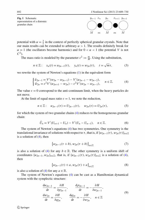
We consider an infinite granular chain of spherical beads of alternating masses (adiatomic granular chain). The physical configuration of the diatomic chain is shownon Fig. 1. Dynamics of the granular beads of alternating masses obey the classicalNewton equations of motion,
{mxn = V ′(yn − xn) − V ′(xn − yn−1),
Myn = V ′(xn+1 − yn) − V ′(yn − xn),n ∈ Z, (1)
where m and M are masses of light and heavy beads, whereas {xn}n∈Z and {yn}n∈Z
are deviations of the beads coordinates from their reference positions. The interactionpotential V represents the Hertzian contact forces for perfect spheres and is given by
V (x) = 1
1 + α|x|1+αH(−x), (2)
where α = 32 and H is the Heaviside step function with H(x) = 1 for x > 0 and
H(x) = 0 for x ≤ 0. See review Sen et al. (2008) for a derivation of the Hertzian
692 J Nonlinear Sci (2013) 23:689–730
Fig. 1 Schematicrepresentation of a diatomicgranular chain
potential with α = 32 in the context of perfectly spherical granular crystals. Note that
our main results can be extended to arbitrary α > 1. The results definitely break forα = 1 (the oscillators become harmonic) and for 0 < α < 1 (the potential V is notC2).
The mass ratio is modeled by the parameter ε2 := mM
. Using the substitution,
n ∈ Z : xn(t) = u2n−1(τ ), yn(t) = w2n(τ ), t = √mτ, (3)
we rewrite the system of Newton’s equations (1) in the equivalent form{
u2n−1 = V ′(w2n − u2n−1) − V ′(u2n−1 − w2n−2),
w2n = ε2V ′(u2n+1 − w2n) − ε2V ′(w2n − u2n−1),n ∈ Z. (4)
The value ε = 0 correspond to the anti-continuum limit, when the heavy particles donot move.
At the limit of equal mass ratio ε = 1, we note the reduction,
n ∈ Z : u2n−1(τ ) = U2n−1(τ ), w2n(τ ) = U2n(τ ), (5)
for which the system of two granular chains (4) reduces to the homogeneous granularchain:
Un = V ′(Un+1 − Un) − V ′(Un − Un−1), n ∈ Z. (6)
The system of Newton’s equations (4) has two symmetries. One symmetry is thetranslational invariance of solutions with respect to τ , that is, if {u2n−1(τ ),w2n(τ )}n∈Z
is a solution of (4), then{u2n−1(τ + b),w2n(τ + b)
}n∈Z
(7)
is also a solution of (4) for any b ∈ R. The other symmetry is a uniform shift ofcoordinates {u2n−1,w2n}n∈Z, that is, if {u2n−1(τ ),w2n(τ )}n∈Z is a solution of (4),then {
u2n−1(τ ) + a,w2n(τ ) + a}n∈Z
(8)
is also a solution of (4) for any a ∈ R.The system of Newton’s equations (4) can be cast as a Hamiltonian dynamical
system with the symplectic structure:
du2n−1
dt= ∂H
∂p2n−1,
dp2n−1
dt= − ∂H
∂u2n−1,
dw2n
dt= ∂H
∂q2n
,dq2n
dt= − ∂H
∂w2n
, n ∈ Z
(9)
J Nonlinear Sci (2013) 23:689–730 693
and the Hamiltonian function
H = 1
2
∑n∈Z
(p2
2n−1 + ε2q22n
) +∑n∈Z
V (w2n − u2n−1) +∑n∈Z
V (u2n−1 − w2n−2), (10)
written in canonical variables {u2n−1,p2n−1 = u2n−1,w2n, q2n = w2n/ε2}n∈Z.
2.2 Periodic Traveling Waves
We shall consider 2π -periodic solutions of the diatomic granular chain (4) satisfying
u2n−1(τ ) = u2n−1(τ + 2π), w2n(τ ) = w2n(τ + 2π), τ ∈ R, n ∈ Z. (11)
Traveling waves correspond to the special solution to the system of Newton’s equa-tions (4), which satisfies the following reduction:
u2n+1(τ ) = u2n−1(τ + 2q), w2n+2(τ ) = w2n(τ + 2q), τ ∈ R, n ∈ Z, (12)
where q ∈ [0,π] is a free parameter. We note that the constraints (11) and (12) implythat there exist 2π -periodic functions u∗ and w∗ such that
u2n−1(τ ) = u∗(τ + 2qn), w2n(τ ) = w∗(τ + 2qn), τ ∈ R, n ∈ Z. (13)
In this context, q is inverse proportional to the wavelength of the periodic travelingwave over the chain n ∈ Z. The functions u∗ and w∗ satisfy the following system ofdifferential advance–delay equations:
{u∗(τ ) = V ′(w∗(τ ) − u∗(τ )) − V ′(u∗(τ ) − w∗(τ − 2q)),
w∗(τ ) = ε2V ′(u∗(τ + 2q) − w∗(τ )) − ε2V ′(w∗(τ ) − u∗(τ )),τ ∈ R. (14)
Remark 1 A more general traveling periodic wave can be sought in the form
u2n−1(τ ) = u∗(cτ + 2qn), w2n(τ ) = w∗(cτ + 2qn), τ ∈ R, n ∈ Z,
where c > 0 is an arbitrary parameter. However, the parameter c can be normalizedto one thanks to invariance of the system of Newton’s equations (4) with the Hertzianpotential (2) with respect to a scaling transformation.
Remark 2 For particular values q = πmN
, where m and N are positive integers suchthat 1 ≤ m ≤ N , periodic traveling waves satisfy a system of 2mN second-orderdifferential equations that follow from the system of lattice differential equations (4)subject to the periodic conditions:
u−1 = u2mN−1, u2mN+1 = u1, w0 = w2mN, w2mN+2 = w2. (15)
This reduction is useful for analysis of stability of periodic traveling waves and fornumerical approximations.
694 J Nonlinear Sci (2013) 23:689–730
2.3 Anti-continuum Limit
Let ϕ be a solution of the nonlinear oscillator equation,
ϕ = V ′(−ϕ) − V ′(ϕ) ⇒ ϕ + |ϕ|α−1ϕ = 0. (16)
Because α = 32 , bootstrapping arguments show that if there exists a classical 2π -
periodic solution of the differential equation (16), then ϕ ∈ C3per(0,2π).
The nonlinear oscillator equation (16) has the first integral
E = 1
2ϕ2 + 1
1 + α|ϕ|α+1. (17)
The phase portrait of the nonlinear oscillator (16) on the (ϕ, ϕ)-plane consists ofa family of closed orbits around the only equilibrium point (0,0). Each orbit cor-responds to the T -periodic solution for ϕ, where T is determined uniquely by en-ergy E. It is well-known (James 2012; Yoshimura 2011) that, for α > 1, the periodT is a monotonically decreasing function of E such that T → ∞ as E → 0 andT → 0 as E → ∞. Therefore, there exists a unique E0 ∈ R+ such that T = 2π forthis E = E0. We also know that the nonlinear oscillator (16) is non-degenerate in thesense that T ′(E0) = 0 (to be more precise, T ′(E0) < 0).
In what follows, we only consider 2π -periodic functions ϕ which are definedby (17) for E = E0. For uniqueness arguments, we shall consider initial conditionsϕ(0) = 0 and ϕ(0) > 0, which determine uniquely one of the two odd 2π -periodicfunctions ϕ.
The limiting 2π -periodic traveling wave solution at ε = 0 should satisfy the con-straints (12), which we do by choosing, for any fixed q ∈ [0,π],
ε = 0 : u2n−1(τ ) = ϕ(τ + 2qn), w2n(τ ) = 0, τ ∈ R, n ∈ Z. (18)
To prove the persistence of this limiting solution with respect to the mass ratio pa-rameter ε2, we shall work in the Sobolev spaces of odd 2π -periodic functions for{u2n−1}n∈Z,
Hku = {
u ∈ Hkper(0,2π) : u(−τ) = −u(τ), τ ∈ R
}, k ∈ N0, (19)
and in the Sobolev spaces of 2π -periodic functions with zero mean for {w2n}n∈Z,
Hkw =
{w ∈ Hk
per(0,2π) :∫ 2π
0w(τ)dτ = 0
}, k ∈ N0. (20)
The constraints in (19) and (20) reflects the presence of the two symmetries (7) and(8). The two symmetries generate a two-dimensional kernel of the linearized opera-tors. Under the constraints in (19) and (20), the kernel of the linearized operators istrivial, zero-dimensional.
It will be clear from analysis that the vector space Hkw defined by (20) is not precise
enough to prove the persistence of traveling wave solutions satisfying the constraints
J Nonlinear Sci (2013) 23:689–730 695
(12). Instead of this space, for any fixed q ∈ [0,π], we introduce the vector space H kw
by
H kw = {
w ∈ Hkper(0,2π) : w(τ) = −w(−τ − 2q)
}, k ∈ N0. (21)
We note that H kw ⊂ Hk
w , because if the constraint w(τ) = −w(−τ − 2q) is satisfied,then the 2π -periodic function w has zero mean. We also note that symmetry con-straint in H k
w can be written as a shifted version of the symmetry constraint in Hku :
w(τ − q) = −w(−τ − q). Although this constraint is not induced directly by thesymmetries (7) and (8), we find that it provides a sufficient frame for application ofthe Implicit Function Theorem.
2.4 Special Periodic Traveling Waves
Before developing persistence analysis, we shall point out three remarkable explicitperiodic traveling solutions of the diatomic granular chain (4) for q = 0, q = π
2 andq = π . For q = π
2 , we have an exact solution
q = π
2: u2n−1(τ ) = ϕ(τ + πn), w2n(τ ) = 0. (22)
This solution preserves the constraint V ′(u2n+1) = V ′(−u2n−1) in the system ofNewton’s equations (4) thanks to the symmetry ϕ(τ − π) = ϕ(τ + π) = −ϕ(τ) ofthe 2π -periodic solution of the nonlinear oscillator equation (16).
For either q = 0 or q = π , we obtain another exact solution,
q = {0,π} : u2n−1(τ ) = ϕ(τ)
(1 + ε2)3, w2n(τ ) = −ε2ϕ(τ)
(1 + ε2)3. (23)
By construction, these solutions (22) and (23) persist for any ε ≥ 0. We shallinvestigate if the continuations are unique near ε = 0 for these special values of q
and if there exists a unique continuation of the general limiting solution (18) in ε forany other fixed value of q ∈ [0,π].
Furthermore, we note that the exact solution (23) for q = π at ε = 1 satisfies theconstraint (5) with U2n−1(τ ) = −U2n(τ ) = U2n(τ −π). This reduction indicates thatthe periodic traveling wave solution (23) for q = π and ε = 1 satisfies the homoge-neous granular chain (6) and coincides with the solution considered by James (2012).On the other hand, the exact solutions (22) for q = π
2 and (23) for q = 0 do not pro-duce any solutions of the homogeneous granular chain at ε = 1. This fact implies thatthere exist generally two distinct solutions at ε = 1, one is continued from ε = 0 andthe other one is constructed from the solution of the homogeneous granular chain (6)in James (2012).
696 J Nonlinear Sci (2013) 23:689–730
3 Persistence of Periodic Traveling Waves Near ε = 0
3.1 Main Result
We consider the system of differential advance–delay equations (14). The limitingsolution (18) becomes now
ε = 0 : u∗(τ ) = ϕ(τ), w∗(τ ) = 0, τ ∈ R, (24)
where ϕ is a unique odd 2π -periodic solution of the nonlinear oscillator equation (16)with ϕ(0) > 0. We now formulate the main result of this section.
Theorem 1 Fix q ∈ [0,π]. There is a unique C1 continuation of 2π -periodic travel-ing wave (24) in ε2, that is, there is a ε0 > 0 such that for every ε ∈ (0, ε0), there area positive constant C and a unique 2π -periodic solution (u∗,w∗) ∈ H 2
u × H 2w of the
system of differential advance–delay equations (14) such that
‖u∗ − ϕ‖H 2per
+ ‖w∗‖H 2per
≤ Cε2. (25)
Remark 3 By Theorem 1, the limiting solution (24) for q ∈ {0, π2 ,π} is uniquely
continued in ε. These continuations coincide with the exact solutions (22) and (23).
3.2 Formal Expansions in Powers of ε
Let us first consider formal expansions in powers of ε to understand the persistenceanalysis from ε = 0. Expanding the solution of the differential advance–delay equa-tions (14), we write
u∗(τ ) = ϕ(τ) + ε2u(2)∗ (τ ) + o(ε2), w∗(τ ) = ε2w(2)∗ (τ ) + o
(ε2), (26)
and obtain the linear inhomogeneous equations
w(2)∗ (τ ) = F (2)w (τ ) := V ′(ϕ(τ + 2q)
) − V ′(−ϕ(τ))
(27)
and
u(2)∗ (τ ) + α∣∣ϕ(τ)
∣∣α−1u(2)∗ (τ )
= F (2)u (τ ) := V ′′(−ϕ(τ)
)w(2)∗ (τ ) + V ′′(ϕ(τ)
)w(2)∗ (τ − 2q). (28)
Because V is C2 but not C3, we have to truncate the formal expansion (26) at o(ε2)
to indicate that there are obstacles to continue the power series beyond terms of theO(ε2) order.
Let us consider two differential operators
L0 = d2
dτ 2: H 2
per(0,2π) → L2per(0,2π), (29)
J Nonlinear Sci (2013) 23:689–730 697
L = d2
dτ 2+ α
∣∣ϕ(τ)∣∣α−1 : H 2
per(0,2π) → L2per(0,2π). (30)
As a consequence of two symmetries, these operators are not invertible because theyadmit one-dimensional kernels,
Ker(L0) = span{1}, Ker(L) = span{ϕ}. (31)
Note that the kernel of L is one-dimensional under the constraint T ′(E0) = 0 (seeLemma 3 in James (2012) for a review of this standard result).
To find uniquely solutions of the inhomogeneous equations (27) and (28) in func-tion spaces H 2
w and H 2u , respectively, see (19) and (20) for definition of function
spaces, the source terms must satisfy the Fredholm conditions
⟨1,F (2)
w
⟩L2
per= 0 and
⟨ϕ,F (2)
u
⟩L2
per= 0.
The first Fredholm condition is satisfied,
∫ 2π
0
[V ′(ϕ(τ + 2q)
) − V ′(−ϕ(τ))]
dτ
=∫ 2π
0V ′(ϕ(τ + 2q)
)dτ −
∫ 2π
0V ′(−ϕ(τ)
)dτ = 0,
because the mean value of a periodic function is independent on the limits of inte-gration and the function ϕ is odd in τ . Since F
(2)w ∈ L2
w , there is a unique solutionw(2) ∈ H 2
w of the linear inhomogeneous equation (27).The second Fredholm condition is satisfied,
∫ 2π
0ϕ(τ )
[V ′′(−ϕ(τ)
)w(2)∗ (τ ) + V ′′(ϕ(τ)
)w(2)∗ (τ − 2q)
]dτ = 0,
if the function F(2)u is odd in τ . If this is the case, then F
(2)u ∈ L2
u and there is a unique
solution u(2) ∈ H 2u of the linear inhomogeneous equation (28). To show that F
(2)u is
odd in τ , we will prove that w(2)∗ satisfies the reduction
w(2)∗ (τ ) = −w(2)∗ (−τ − 2q) ⇒ F (2)u (−τ) = −F (2)
u (τ ), τ ∈ R. (32)
It follows from the linear inhomogeneous equation (27) that
w(2)∗ (τ ) + w(2)∗ (−τ − 2q) = V ′(ϕ(τ + 2q)) − V ′(−ϕ(τ)
) + V ′(ϕ(−τ))
− V ′(−ϕ(−τ − 2q)) = 0,
where the last equality appears because ϕ is odd in τ . Integrating this equation twiceand using the fact that w
(2)∗ ∈ H 2w , we obtain reduction (32). Note that the reduction
(32) implies that w(2)∗ ∈ H 2
w , where H 2w ⊂ H 2
w is given by (21).
698 J Nonlinear Sci (2013) 23:689–730
3.3 Proof of Theorem 1
To prove Theorem 1, we shall consider the vector fields of the differential advance–delay equations (14),
{Fu(u(τ),w(τ)) := V ′(w(τ) − u(τ)) − V ′(u(τ ) − w(τ − 2q)),
Fw(u(τ),w(τ), ε) := ε2V ′(u(τ + 2q) − w(τ)) − ε2V ′(w(τ) − u(τ)).(33)
We are looking for a strong solution (u∗,w∗) of the system (14) satisfying the reduc-tion,
u∗(−τ) = −u∗(τ ), w∗(τ ) = −w∗(−τ − 2q), τ ∈ R, (34)
that is, u∗ ∈ H 2u (R) and w∗ ∈ H 2
w(R).If (u,w) ∈ H 2
u × H 2w , then Fu is odd in τ . Furthermore, since V is C2, then Fu is
a C1 map from H 2u × H 2
w to L2u and its Jacobian at w = 0 is given by
DuFu(u,0) = −V ′′(−u) − V ′′(u) = −α|u|α−1,
DwFu(u,0) = V ′′(−u) − V ′′(u) = α|u|α−1sign(u).
On the other hand, under the constraints (34), we have Fw ∈ L2w , because
∫ 2π
0Fw
(u(τ),w(τ), ε
)dτ = ε2
∫ 2π
0V ′(u(τ + 2q) + w(−τ − 2q)
)dτ
− ε2∫ 2π
0V ′(w(τ) + u(−τ)
)dτ = 0.
Moreover, under the constraints (34), we actually have Fw ∈ L2w because
Fw
(u(τ),w(τ), ε
) + Fw
(u(−τ − 2q),w(−τ − 2q), ε
)= ε2V ′(u(τ + 2q) − w(τ)
) − ε2V ′(w(τ) − u(τ))
+ ε2V ′(u(−τ) − w(−τ − 2q)) − ε2V ′(w(−τ − 2q) − u(−τ − 2q)
)= 0.
Since V is C2, then Fw is a C1 map from H 2u × H 2
w to L2w . We also note that
Fw(u,w, ε) = ε2Fw(u,w), where Fw(u,w) is ε-independent.Let us now define the nonlinear operator
⎧⎨⎩
fu(u,w, ε) := d2u
dτ 2 − Fu(u,w),
fw(u,w, ε) := d2w
dτ 2 − ε2Fw(u,w).(35)
The nonlinear operator (fu, fw) : H 2u × H 2
w × R → L2u × L2
w is C1 near the point(ϕ,0,0) ∈ H 2
u × H 2w × R. To apply the Implicit Function Theorem near this point,
we need (fu, fw) = (0,0) at (u,w, ε) = (ϕ,0,0) and the invertibility of the Jacobianoperator (fu, fw) with respect to (u,w) near (ϕ,0,0).
J Nonlinear Sci (2013) 23:689–730 699
The Jacobian operator of (fu, fw) at (ϕ,0,0) is given by the matrix
[L α|ϕ|α−1sign(ϕ)
0 L0
],
where operators L and L0 are defined by (29) and (30). The kernels of these opera-tors in (31) are zero-dimensional in the constrained vector spaces (19) and (20) (weactually use space (21) in place of space (20)).
By the Implicit Function Theorem, there exists a C1 continuation of the limitingsolution (24) with respect to ε2 as the 2π -periodic solutions (u∗,w∗) ∈ H 2
u × H 2w
of the system of differential advance–delay equations (14) near ε = 0. The proof ofTheorem 1 is complete.
4 Spectral Stability of Periodic Traveling Waves Near ε = 0
4.1 Linearization at the Periodic Traveling Waves
We shall consider the diatomic granular chain (4), which admits for small ε > 0 theperiodic traveling waves in the form (13), where (u∗,w∗) is defined by Theorem 1.Linearizing the system of nonlinear equations (4) at the periodic traveling waves (13),we obtain the system of linearized equations for small perturbations,
⎧⎪⎪⎨⎪⎪⎩
u2n−1 = V ′′(w∗(τ + 2qn) − u∗(τ + 2qn))(w2n − u2n−1)
− V ′′(u∗(τ + 2qn) − w∗(τ + 2qn − 2q))(u2n−1 − w2n−2),
w2n = ε2V ′′(u∗(τ + 2qn + 2q) − w∗(τ + 2qn))(u2n+1 − w2n)
− ε2V ′′(w∗(τ + 2qn) − u∗(τ + 2qn))(w2n − u2n−1),
(36)
where n ∈ Z. A technical complication is that V ′′ is continuous but not continuousdifferentiable. This will complicate our analysis of perturbation expansions for smallε > 0. Note that the technical complications do not occur for the exact solutions (22)and (23). Indeed, for the exact solution (22) with q = π
2 , the linearized system (36) isrewritten explicitly as
{u2n−1 + α|ϕ|α−1u2n−1 = V ′′(−ϕ)w2n + V ′′(ϕ)w2n−2,
w2n + 2ε2V ′′(−ϕ)w2n = ε2V ′′(−ϕ)(u2n+1 + u2n−1).(37)
For the exact solution (23) with q = 0 or q = π , the linearized system (36) is rewrittenexplicitly as
{u2n−1 + α
1+ε2 |ϕ|α−1u2n−1 = 11+ε2 (V ′′(−ϕ)w2n + V ′′(ϕ)w2n−2),
w2n + αε2
1+ε2 |ϕ|α−1w2n = ε2
1+ε2 (V ′′(ϕ)u2n+1 + V ′′(−ϕ)u2n−1).(38)
In both cases, the linearized systems (37) and (38) are analytic in ε near ε = 0.
700 J Nonlinear Sci (2013) 23:689–730
The system of linearized equations (36) has the same symplectic structure (9), butthe Hamiltonian function is now given by
H = 1
2
∑n∈Z
(p2
2n−1 + ε2q22n
)
+ 1
2
∑n∈Z
V ′′(w∗(τ + 2qn) − u∗(τ + 2qn))(w2n − u2n−1)
2
+ 1
2
∑n∈Z
V ′′(u∗(τ + 2qn) − w∗(τ + 2qn − 2q))(u2n−1 − w2n−2)
2. (39)
The Hamiltonian H is quadratic in canonical variables {u2n−1,p2n−1 = u2n−1,w2n,
q2n = w2n/ε2}n∈Z.
4.2 Main Result
Because coefficients of the linearized equations (36) are 2π -periodic in τ , we shalllook for an infinite-dimensional analog of the Floquet theorem that states that allsolutions of the linear system with 2π -periodic coefficients satisfies the reduction
u(τ + 2π) = Mu(τ ), τ ∈ R, (40)
where u := [. . . ,w2n−2, u2n−1,w2n,u2n+1, . . .] and M is the monodromy operator.Eigenvalues of the monodromy operator M denoted by μ are called the Floquetmultipliers.
Remark 4 Let q = πmN
for some positive integers m and N such that 1 ≤ m ≤ N . Inthis case, the system of nonlinear equations (4) can be closed into a chain of 2mN
second-order differential equations subject to the periodic boundary conditions (15).Similarly, the system of linearized equations (36) can also be closed as a system of2mN second-order equations and the monodromy operator M becomes an infinitediagonal composition of an identical 4mN -by-4mN Floquet matrix.
We can find eigenvalues of the monodromy operator M by looking for the set ofeigenvectors in the form,
u2n−1(τ ) = U2n−1(τ )eλτ , w2n(τ ) = εW2n(τ )eλτ , τ ∈ R, (41)
where (U2n−1,W2n) are 2π -periodic functions and the admissible values of λ arefound from the existence of these 2π -periodic functions. The admissible values of λ
are called the characteristic exponents and they define the Floquet multipliers μ bythe standard formula μ = e2πλ.
J Nonlinear Sci (2013) 23:689–730 701
Eigenvectors (41) are defined as 2π -periodic solutions of the linear eigenvalueproblem,
⎧⎪⎪⎪⎪⎪⎪⎨⎪⎪⎪⎪⎪⎪⎩
U2n−1 + 2λU2n−1 + λ2U2n−1= V ′′(w∗(τ + 2qn) − u∗(τ + 2qn))(εW2n − U2n−1)
− V ′′(u∗(τ + 2qn) − w∗(τ + 2qn − 2q))(U2n−1 − εW2n−2),
W2n + 2λW2n + λ2W2n
= εV ′′(u∗(τ + 2qn + 2q) − w∗(τ + 2qn))(U2n+1 − εW2n)
− εV ′′(w∗(τ + 2qn) − u∗(τ + 2qn))(εW2n − U2n−1).
(42)
Associated with simple imaginary characteristic exponents λ ∈ iR, we define theKrein signature of such eigenvalues as the sign of the 2-form associated with thesymplectic structure (9):
σ = i∑n∈Z
[u2n−1p2n−1 − u2n−1p2n−1 + w2nq2n − w2nq2n], (43)
where {u2n−1,p2n−1 = u2n−1,w2n, q2n = w2n/ε2}n∈Z is obtained from the corre-
sponding eigenvector (41). By the symmetry of the linear eigenvalue problem (42), itfollows that if λ is an eigenvalue, then λ is also an eigenvalue, whereas the 2-form σ
is constant with respect to τ ∈ R.
Remark 5 The Krein signature plays an important role in the studies of spectralstability of periodic solutions (see Sect. 4 in Aubry 1997). In particular, instabili-ties associated with complex characteristic exponents with Re(λ) > 0 typically arisewhen two imaginary characteristic exponents λ with opposite Krein signatures coa-lesce (Bridges 1990; MacKay 1986; Vougalter and Pelinovsky 2006). The count ofeigenvalues of different Krein signatures is also important for the control of the totalnumber of unstable eigenvalues in Hamiltonian dynamical systems (Chugunova andPelinovsky 2010; Kapitula et al. 2004; Pelinovsky 2005).
If ε = 0, the monodromy operator M in (40) is block-diagonal and consists ofan infinite set of 2-by-2 Jordan blocks, because the diatomic granular chain (4) isdecoupled into a countable set of uncoupled second-order differential equations. Asa result, the linear eigenvalue problem (42) with the limiting solution (24) admits aninfinite set of 2π -periodic solutions for λ = 0,
ε = 0 : U(0)2n−1 = c2n−1ϕ(τ + 2qn), W
(0)2n = a2n, n ∈ Z, (44)
where {c2n−1, a2n}n∈Z are arbitrary coefficients. Besides eigenvectors (44), thereexists another countable set of generalized eigenvectors for each of the uncoupledsecond-order differential equations, which contribute to 2-by-2 Jordan blocks. Eachblock corresponds to the double Floquet multiplier μ = 1 or the double character-istic exponent λ = 0. When ε = 0 but ε � 1, the characteristic exponent λ = 0 ofa high algebraic multiplicity splits. We shall study the splitting of the characteristicexponents λ by the perturbation arguments.
We now formulate the main result of this section.
702 J Nonlinear Sci (2013) 23:689–730
Theorem 2 Fix q = πmN
for some positive integers m and N such that 1 ≤ m ≤ N .
Let (u∗,w∗) ∈ H 2u × H 2
w be defined by Theorem 1 for sufficiently small positive ε.Consider the linear eigenvalue problem (42) subject to 2mN -periodic boundaryconditions (15). There is a ε0 > 0 such that, for every ε ∈ (0, ε0), there existsq0(ε) ∈ (0, π
2 ) such that for every q ∈ (0, q0(ε)) or q ∈ (π − q0(ε),π], no valuesof λ with Re(λ) = 0 exist, whereas for every q ∈ (q0(ε),π − q0(ε)), there exist char-acteristic values of λ with Re(λ) > 0.
Remark 6 By Theorem 2, periodic traveling waves are spectrally stable for q ∈(0, q0(ε)) and q ∈ (π − q0(ε),π] and unstable for q ∈ (q0(ε),π − q0(ε)). The nu-merical value of q0(ε) as ε → 0 is q0(0) ≈ 0.915. Therefore, the linearized system(37) for the exact solution (22) with q = π
2 subject to 4-periodic boundary conditions(m = 1 and N = 2) is unstable for small ε > 0, whereas the linearized system (38) forthe exact solution (23) with q = π subject to 2-periodic boundary conditions (m = 1and N = 1) is stable for small ε > 0.
Remark 7 The result of Theorem 2 is expected to hold for all values of q in [0,π]but the spectrum of the linear eigenvalue problem (42) for the characteristic expo-nent λ becomes continuous and the spectral band is connected to zero. An infinite-dimensional analog of perturbation theory is required to study the eigenvalues of themonodromy operator M in this case.
Remark 8 The case q = 0 is degenerate for an application of the perturbation the-ory. Nevertheless, we show numerically that the linearized system (38) for the exactsolution (23) with q = 0 (m = 1 and N → ∞) is stable for small ε > 0 and all char-acteristic exponents are at least double for any ε > 0.
4.3 Formal Perturbation Expansions
We would normally expect splitting λ = O(ε1/2) if the limiting linear eigenvalueproblem at ε = 0 is diagonally decomposed into 2-by-2 Jordan blocks (Pelinovskyand Sakovich 2012). However, in the linearized diatomic granular chain (42), thissplitting occurs in a higher order, that is, λ = O(ε), because the coupling betweenthe particles of equal masses shows up at the O(ε2) order of the perturbation theory.Regular perturbation computations in O(ε2) would require V ′′ to be at least C1,which we do not have. In the computations below, we neglect this obstacle, which ispossible for at least q = π
2 and q = π . For other values of q , the formal perturbationexpansion of this section will be justified in Sect. 4.7 with a kind of renormalizationtechnique.
Expanding 2π -periodic solutions of the linear eigenvalue problem (42), we write
λ = ελ(1) + ε2λ(2) + o(ε2) (45)
and {U2n−1 = U
(0)2n−1 + εU
(1)2n−1 + ε2U
(2)2n−1 + o(ε2),
W2n = W(0)2n + εW
(1)2n + ε2W
(2)2n + o(ε2),
(46)
J Nonlinear Sci (2013) 23:689–730 703
where the zeroth-order terms are given by (44). To determine corrections of theseexpansions uniquely, we shall require that
⟨ϕ,U
(j)
2n−1
⟩L2
per= ⟨
1,W(j)
2n
⟩L2
per= 0, n ∈ Z, j = 1,2. (47)
Indeed, if U(j)
2n−1 contains a component, which is parallel to ϕ, then the correspondingterm only changes the value of c2n−1 in the eigenvector (44), which is yet to bedetermined. Similarly, if a 2π -periodic function W
(j)
2n has a nonzero mean value,
then the mean value of W(j)
2n only changes the value of a2n in the eigenvector (44),which is yet to be determined.
The linearized equations (42) are satisfied at the O(ε0) order. Collecting terms atthe O(ε) order, we obtain
⎧⎪⎪⎪⎨⎪⎪⎪⎩
U(1)2n−1 + α|ϕ(τ + 2qn)|α−1U
(1)2n−1
= −2λ(1)U(0)2n−1 + V ′′(−ϕ(τ + 2qn))W
(0)2n + V ′′(ϕ(τ + 2qn))W
(0)2n−2,
W(1)2n = −2λ(1)W
(0)2n + V ′′(ϕ(τ + 2qn + 2q))U
(0)2n+1
+ V ′′(−ϕ(τ + 2qn))U(0)2n−1.
(48)
Let us define solutions of the following linear inhomogeneous equations:
v + α|ϕ|α−1v = −2ϕ, (49)
y± + α|ϕ|α−1y± = V ′′(±ϕ), (50)
z± = V ′′(±ϕ)ϕ. (51)
If we can find uniquely 2π -periodic solutions of these equations such that
〈ϕ, v〉L2per
= 〈ϕ, y±〉L2per
= 〈1, z±〉L2per
= 0,
then the perturbation equations (48) at the O(ε) order are satisfied with the solution:{
U(1)2n−1 = c2n−1λ
(1)v(τ + 2qn) + a2ny−(τ + 2qn) + a2n−2y+(τ + 2qn),
W(1)2n = c2n+1z+(τ + 2qn + 2q) + c2n−1z−(τ + 2qn).
(52)
The linearized equations (42) are now satisfied up to the O(ε) order. Collectingterms at the O(ε2) order, we obtain
⎧⎪⎪⎪⎪⎪⎪⎪⎪⎪⎪⎪⎪⎨⎪⎪⎪⎪⎪⎪⎪⎪⎪⎪⎪⎪⎩
U(2)2n−1 + α|ϕ(τ + 2qn)|α−1U
(2)2n−1
= −2λ(1)U(1)2n−1 − 2λ(2)U
(0)2n−1 − (λ(1))2U
(0)2n−1
+ V ′′(−ϕ(τ + 2qn))W(1)2n + V ′′(ϕ(τ + 2qn))W
(1)2n−2
− V ′′′(−ϕ(τ + 2qn))(w(2)∗ (τ + 2qn) − u
(2)∗ (τ + 2qn))U(0)2n−1
− V ′′′(ϕ(τ + 2qn))(u(2)∗ (τ + 2qn) − w
(2)∗ (τ + 2qn − 2q))U(0)2n−1,
W(2)2n = −2λ(1)W
(1)2n − 2λ(2)W
(0)2n − (λ(1))2W
(0)2n
+ V ′′(ϕ(τ + 2qn + 2q))(U(1)2n+1 − W
(0)2n )
+ V ′′(−ϕ(τ + 2qn))(U(1)2n−1 − W
(0)2n ),
(53)
704 J Nonlinear Sci (2013) 23:689–730
where corrections u(2)∗ and w
(2)∗ are defined by expansion (26).To solve the linear inhomogeneous equations (53), the source terms have to satisfy
the Fredholm conditions because both operators L and L0 defined by (29) and (30)have one-dimensional kernels. Therefore, we require the first equation of system (53)to be orthogonal to ϕ and the second equation of system (53) to be orthogonal to1 on [−π,π]. Substituting (44) and (52) to the orthogonality conditions and takinginto account the symmetry between couplings of lattice sites on Z, we obtain thedifference equations for {c2n−1, a2n}n∈Z:
{KΛ2c2n−1 = M1(c2n+1 + c2n−3 − 2c2n−1) + L1Λ(a2n − a2n−2),
Λ2a2n = M2(a2n+2 + a2n−2 − 2a2n) + L2Λ(c2n+1 − c2n−1),(54)
where Λ ≡ λ(1), and (K,M1,M2,L1,L2) are numerical coefficients to be computedfrom the projections. In particular, we obtain
K =∫ π
−π
(2v(τ ) + ϕ(τ )
)ϕ(τ )dτ,
M1 =∫ π
−π
V ′′(−ϕ(τ))ϕ(τ )z+(τ + 2q)dτ =
∫ π
−π
V ′′(ϕ(τ))ϕ(τ )z−(τ − 2q)dτ,
M2 = 1
2π
∫ π
−π
V ′′(ϕ(τ + 2q))y−(τ + 2q)dτ = 1
2π
∫ π
−π
V ′′(−ϕ(τ))y+(τ )dτ,
L1 = −2∫ π
−π
y−(τ )ϕ(τ )dτ = 2∫ π
−π
y+(τ )ϕ(τ )dτ,
L2 = 1
2π
∫ π
−π
V ′′(ϕ(τ + 2q))v(τ + 2q)dτ = − 1
2π
∫ π
−π
V ′′(−ϕ(τ))v(τ)dτ.
Note that the coefficients M1 and M2 need not to be computed at the diagonalterms c2n−1 and a2n thanks to the fact that the difference equations (54) with Λ = 0must have eigenvectors with equal values of {c2n−1}n∈Z and {a2n}n∈Z, which corre-spond to the two symmetries of the system of linearized equations (36) related to thesymmetries (7) and (8). This fact shows that the problem of limited smoothness ofV ′′, which is C but not C1 near zero, is not a serious obstacle in the derivation ofthe reduced system (54). Indeed, we show in Sect. 4.7 how to fix the perturbationexpansion and to avoid this obstacle.
Difference equations (54) give a necessary and sufficient condition to solve thelinear inhomogeneous equations (53) at the O(ε2) order and to continue the perturba-tion expansions beyond this order. Before justifying this formal perturbation theory,we shall explicitly compute the coefficients (K,M1,M2,L1,L2) of the differenceequations (54).
Note that the system of difference equations (54) presents a quadratic eigenvalueproblem with respect to the spectral parameter Λ. Such quadratic eigenvalue problemappear often in the context of spectral stability of nonlinear waves (Chugunova andPelinovsky 2009; Kollar 2011).
J Nonlinear Sci (2013) 23:689–730 705
4.4 Explicit Computations of the Coefficients
We shall prove the following technical result.
Lemma 1 Coefficients K , M2, L1, and L2 are independent of q and are given by
K = − 4π2
T ′(E0), M2 = 2
πT ′(E0)(ϕ(0))2,
L1 = 2πL2 = 2(2π − T ′(E0)(ϕ(0))2)
T ′(E0)ϕ(0).
Consequently, K > 0, whereas M2,L1,L2 < 0. On the other hand, coefficient M1depends on q and is given by
M1 = − 2
π
(ϕ(0)
)2 + I (q),
where
I (q) = I (π − q) := −∫ π
π−2q
ϕ(τ )ϕ(τ + 2q)dτ for q ∈[
0,π
2
].
To prove Lemma 1, we first uniquely solve the linear inhomogeneous equations(49), (50), and (51). For Eq. (49), we note that a general solution is
v(τ) = −τ ϕ(τ ) + b1ϕ(τ ) + b2∂EϕE0(τ ), τ ∈ [−π,π],where (b1, b2) are arbitrary constants and ∂EϕE0 is the derivative of the T (E)-periodic solution ϕE of the nonlinear oscillator equation (16) with the first integral(17) satisfying initial conditions ϕE(0) = 0 and ϕE(0) = √
2E at the value of energyE = E0, for which T (E0) = 2π . We note the equation
∂EϕE0(±π) = ∓1
2T ′(E0)ϕ(±π), (55)
that follows from the differentiation of equation ϕE(±T (E)/2) = 0 with respect toE at E = E0.
To define v uniquely, we require that 〈ϕ, v〉L2per
= 0. Because ϕ is even in τ ,whereas τ ϕ and ∂EϕE0 are odd, we hence have b1 = 0 and v(0) = 0. Hence v isodd in τ and, in order to satisfy the 2π -periodicity, we shall only require v(π) = 0,which uniquely specifies the value of b2 by virtue of (55),
b2 = πϕ(π)
∂EϕE0(π)= − 2π
T ′(E0).
As a result, we obtain
v(τ) = −τ ϕ(τ ) − 2π
T ′(E0)∂EϕE0(τ ), τ ∈ [−π,π]. (56)
706 J Nonlinear Sci (2013) 23:689–730
For Eq. (50), we can use ϕ(τ) ≥ 0 for τ ∈ [0,π] and ϕ(τ) ≤ 0 for τ ∈ [−π,0]. Wecan also use the symmetry ϕ(π) = −ϕ(0). Integrating equations for y± separately,we obtain
y+(τ ) ={
1 + a+ϕ + b+∂EϕE0 , τ ∈ [−π,0],c+ϕ + d+∂EϕE0, τ ∈ [0,π],
y−(τ ) ={
a−ϕ + b−∂EϕE0, τ ∈ [−π,0],1 + c−ϕ + d−∂EϕE0 , τ ∈ [0,π].
Continuity of y± and y± across τ = 0 defines uniquely d± = b± and c± = a± ± 1ϕ(0)
.With this definition, y±(−π) = y±(π), whereas condition y±(−π) = y±(π) sets upuniquely
b± = ± 2
T ′(E0)ϕ(0),
whereas constants a± are not specified.To define y± uniquely, we again require that 〈ϕ, y±〉L2
per= 0. This yields the con-
straint on a±,
a± = ∓ 1
2ϕ(0)∓
2〈ϕ, ∂EϕE0〉L2per
T ′(E0)ϕ(0)〈ϕ, ϕ〉L2per
.
As a result, we obtain
y+(τ ) = a+ϕ(τ ) + b+∂EϕE0(τ ) +{
1, τ ∈ [−π,0],ϕ(τ )ϕ(0)
, τ ∈ [0,π], (57)
and
y−(τ ) = a−ϕ(τ ) + b−∂EϕE0(τ ) +{
0, τ ∈ [−π,0],1 − ϕ(τ )
ϕ(0), τ ∈ [0,π], (58)
where (a±, b±) are uniquely defined above.For Eq. (51), we integrate separately on [−π,0] and [0,π] to obtain
z+(τ ) ={
c+ − |ϕ(τ)|α, τ ∈ [−π,0],c+, τ ∈ [0,π],
and
z−(τ ) ={
c−, τ ∈ [−π,0],c− + |ϕ(τ)|α, τ ∈ [0,π],
where (c+, c−) are constants of integration and continuity of z± across τ = 0 havebeen used. To define z± uniquely, we require that 〈1, z±〉L2
per= 0. Integrating the
equations above under this condition, we obtain
z+(τ ) ={
c+τ + d+ − ϕ(τ ), τ ∈ [−π,0],c+τ − d+, τ ∈ [0,π],
J Nonlinear Sci (2013) 23:689–730 707
and
z−(τ ) ={
c−τ + d−, τ ∈ [−π,0],c−τ − d− − ϕ(τ ), τ ∈ [0,π],
where (d+, d−) are constants of integration. Continuity of z± across τ = 0 uniquelysets coefficients d± = ± 1
2 ϕ(0). Periodicity of z±(−π) = z±(π) is satisfied. Period-icity of z±(−π) = z±(π) uniquely defines coefficients c± = ± 1
πϕ(0). As a result,
we obtain
z+(τ ) = 1
2π
{ϕ(0)(2τ + π) − 2πϕ(τ ), τ ∈ [−π,0],ϕ(0)(2τ − π), τ ∈ [0,π], (59)
and
z−(τ ) = 1
2π
{−ϕ(0)(2τ + π), τ ∈ [−π,0],−ϕ(0)(2τ − π) − 2πϕ(τ ), τ ∈ [0,π]. (60)
We can now compute the coefficients (K,M1,M2,L1,L2) of the difference equa-tions (54). For coefficients K , we integrate by parts, use Eqs. (16), (17), (56), andobtain
K =∫ π
−π
ϕ(ϕ + 2v)dτ
=∫ π
−π
(ϕ2 − 2vϕ
)dτ
=[τ ϕ2 + 2π
T ′(E0)∂EϕE0 ϕ
]∣∣∣∣τ=π
τ=−π
+ 2π
T ′(E0)
∫ π
−π
(∂EϕE0 ϕ − ∂EϕE0 ϕ)dτ
= − 4π
T ′(E0)
∫ π
0∂E
(1
2ϕ2 + 1
1 + αϕ1+α
)E0
dτ
= − 4π2
T ′(E0).
Because T ′(E0) < 0, we find that K > 0.For M1, we use Eq. (51), solution (60), and obtain
M1 =∫ π
−π
V ′′(−ϕ(τ))ϕ(τ )z+(τ + 2q)dτ
=∫ π
−π
z−(τ )z+(τ + 2q)dτ
= −∫ π
−π
z−(τ )z+(τ + 2q)dτ
=∫ π
0ϕ(τ )z+(τ + 2q)dτ,
708 J Nonlinear Sci (2013) 23:689–730
hence, the sign of M1 depends on q . Using solution (59), for q ∈ [0, π2 ], we obtain
M1 = 1
πϕ(0)
∫ π
0ϕ(τ )dτ −
∫ π
π−2q
ϕ(τ )ϕ(τ + 2q)dτ
= − 2
π
(ϕ(0)
)2 + I (q),
where
I (q) := −∫ π
π−2q
ϕ(τ )ϕ(τ + 2q)dτ.
On the other hand, for q ∈ [π2 ,π], we obtain
M1 = − 2
π
(ϕ(0)
)2 + I (q),
where
I (q) := −∫ 2π−2q
0ϕ(τ )ϕ(τ + 2q)dτ,
so that
I (π − q) = −∫ 2q
0ϕ(τ )ϕ(τ − 2q)dτ = −
∫ 0
−2q
ϕ(τ )ϕ(τ + 2q)dτ = I (q),
because the mean value of a periodic function does not depend on the limits of inte-gration.
For M2, we use Eq. (50) and obtain
M2 = 1
2π
∫ π
−π
V ′′(−ϕ)y+ dτ
= α
2π
∫ π
0ϕα−1y+ dτ
= − 1
2π
∫ π
0y+ dτ
= 1
πb+∂EφE0(0)
= 2
πT ′(E0)(ϕ(0))2,
hence, M2 < 0.For L1, we use Eqs. (16), (17), (58), and obtain
L1 = −2∫ π
−π
y−ϕ dτ
= −2b−∫ π
−π
∂EϕE0 ϕ dτ
J Nonlinear Sci (2013) 23:689–730 709
= 4
T ′(E0)ϕ(0)
[∫ π
0(∂EϕE0 ϕ − ∂EϕE0 ϕ)dτ + ϕ∂EϕE0
∣∣∣∣τ=π
τ=0
]
= 2(2π − T ′(E0)(ϕ(0))2)
T ′(E0)ϕ(0).
Because ϕ(0) > 0 and T ′(E0) < 0, we find that L1 < 0.For L2, we use Eqs. (16), (17), (56), and obtain
L2 = − 1
2π
∫ π
−π
V ′′(−ϕ)v dτ
= − α
2π
∫ π
0ϕα−1v dτ
= 1
T ′(E0)
∫ π
0∂E(ϕE0)
α dτ − 1
2π
∫ π
0ϕαdτ
=[
1
2πϕ − 1
T ′(E0)∂EϕE0
]∣∣∣∣τ=π
τ=0
= 2π − T ′(E0)(ϕ(0))2
πT ′(E0)ϕ(0)
= 1
2πL1,
hence, L2 < 0.The proof of Lemma 1 is complete.
4.5 Eigenvalues of the Difference Equations
Because the coefficients (K,M1,M2,L1,L2) of the difference equations (54) areindependent of n, we can solve these equations by the discrete Fourier transform.Substituting
c2n−1 = Ceiθ(2n−1), a2n = Aei2θn, (61)
where θ ∈ [0,π] is the Fourier spectral parameter, we obtain the system of linearhomogeneous equations,
{KΛ2C = 2M1(cos(2θ) − 1)C + 2iL1Λ sin(θ)A,
Λ2A = 2M2(cos(2θ) − 1)A + 2iL2Λ sin(θ)C.(62)
A nonzero solution of the linear system (62) exists if and only if Λ is a root of thecharacteristic polynomial,
D(Λ; θ) = KΛ4 + 4Λ2(M1 + KM2 + L1L2) sin2(θ) + 16M1M2 sin4(θ) = 0. (63)
Since this equation is bi-quadratic, it has two pairs of roots for each θ ∈ [0,π]. Forθ = 0, both pairs are zero, which recovers the characteristic exponent λ = 0 of al-gebraic multiplicity of (at least) 4 in the linear eigenvalue problem (42). For a fixed
710 J Nonlinear Sci (2013) 23:689–730
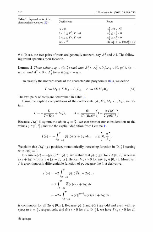
Table 1 Squared roots of thecharacteristic equation (63) Coefficients Roots
Δ < 0 Λ21 < 0 < Λ2
20 < Δ ≤ Γ 2, Γ > 0 Λ2
1 ≤ Λ22 < 0
0 < Δ ≤ Γ 2, Γ < 0 Λ22 ≥ Λ2
1 > 0
Δ > Γ 2 Im(Λ21) > 0, Im(Λ2
2) < 0
θ ∈ (0,π), the two pairs of roots are generally nonzero, say Λ21 and Λ2
2. The follow-ing result specifies their location.
Lemma 2 There exists a q0 ∈ (0, π2 ) such that Λ2
1 ≤ Λ22 < 0 for q ∈ [0, q0) ∪ (π −
q0,π] and Λ21 < 0 < Λ2
2 for q ∈ (q0,π − q0).
To classify the nonzero roots of the characteristic polynomial (63), we define
Γ := M1 + KM2 + L1L2, Δ := 4KM1M2. (64)
The two pairs of roots are determined in Table 1.Using the explicit computations of the coefficients (K,M1,M2,L1,L2), we ob-
tain
Γ = − 8
T ′(E0)+ I (q), Δ = 64
(T ′(E0))2
(1 − πI (q)
2(ϕ(0))2
).
Because I (q) is symmetric about q = π2 , we can restrict our consideration to the
values q ∈ [0, π2 ] and use the explicit definition from Lemma 1:
I (q) = −∫ π
π−2q
ϕ(τ )ϕ(τ + 2q)dτ, q ∈[
0,π
2
].
We claim that I (q) is a positive, monotonically increasing function in [0, π2 ] starting
with I (0) = 0.Because ϕ(τ ) = −|ϕ(τ)|α−1ϕ(τ), we realize that ϕ(τ ) ≤ 0 for τ ∈ [0,π], whereas
ϕ(τ + 2q) ≥ 0 for τ ∈ [π − 2q,π]. Hence, I (q) ≥ 0 for any 2q ∈ [0,π]. Moreover,I is a continuously differentiable function of q , because the first derivative,
I ′(q) = −2∫ π
π−2q
ϕ(τ )...ϕ(τ + 2q)dτ
= 2∫ π
π−2q
...ϕ(τ)ϕ(τ + 2q)dτ
= −2α
∫ π
π−2q
∣∣ϕ(τ)∣∣α−1
ϕ(τ )ϕ(τ + 2q)dτ,
is continuous for all 2q ∈ [0,π]. Because ϕ(τ ) and ϕ(τ ) are odd and even with re-spect to τ = π
2 , respectively, and ϕ(τ ) ≥ 0 for τ ∈ [0, π2 ], we have I ′(q) ≥ 0 for all
J Nonlinear Sci (2013) 23:689–730 711
2q ∈ [0,π]. Therefore, I (q) is monotonically increasing from I (0) = 0 to
I
(π
2
)= −
∫ π
0ϕ(τ )ϕ(τ + π)dτ =
∫ π
0
(ϕ(τ )
)2 dτ > 0.
Hence, for all q ∈ [0, π2 ], we have Γ > 0 and
Γ 2 − Δ = I (q)
(I (q) − 16
T ′(E0)+ 32π
(T ′(E0)ϕ(0))2
)≥ 0,
where Δ = Γ 2 if and only if q = 0. Therefore, only the first two lines of Table 1 canoccur.
For q = 0, I (0) = 0, hence M1 < 0, Δ > 0 and Δ = Γ 2. The second line ofTable 1 gives Λ2
1 = Λ22 < 0. All characteristic exponents are purely imaginary and
degenerate, thanks to the explicit computations:
Λ21 = Λ2
2 = − 4
π2sin2(θ). (65)
The proof of Lemma 2 is achieved if there is q0 ∈ (0, π2 ) such that the first line
of Table 1 yields Λ21 < 0 < Λ2
2 for q ∈ (q0,π2 ] and the second line of Table 2 yields
Λ21 < Λ2
2 < 0 for q ∈ (0, q0). Because I is a monotonically increasing function ofq and Δ > 0 for q = 0, the existence of q0 ∈ (0, π
2 ) follows by continuity if Δ < 0for q = π
2 . Since K > 0 and M2 < 0, we need to prove that M1 > 0 for q = π2 or,
equivalently,
I
(π
2
)>
2
π
(ϕ(0)
)2.
Because ϕ is a 2π -periodic function with zero mean, the Poincaré inequality yields
I
(π
2
)= 1
2
∫ π
−π
(ϕ(τ )
)2 dτ ≥ 1
2
∫ π
−π
(ϕ(τ )
)2 dτ.
On the other hand, using Eqs. (16), (17), and integration by parts, we obtain
1
2
∫ π
−π
(ϕ(τ )
)2 dτ = −1
2
∫ π
−π
ϕ(τ)ϕ(τ )dτ = 1
2
∫ π
−π
∣∣ϕ(τ)∣∣α+1dτ = 2π(α + 1)
(α + 3)E,
where the last equality is obtained by integrating the first invariant (17) on [−π,π].Therefore, we obtain
I
(π
2
)≥ 2π(α + 1)
(α + 3)E = π(α + 1)
(α + 3)
(ϕ(0)
)2>
2
π
(ϕ(0)
)2,
where the last inequality is obtained for α = 32 based on the fact that 5π2
18 ≈ 2.74 > 1.Therefore, M1 > 0 and hence, Δ < 0 for q = π
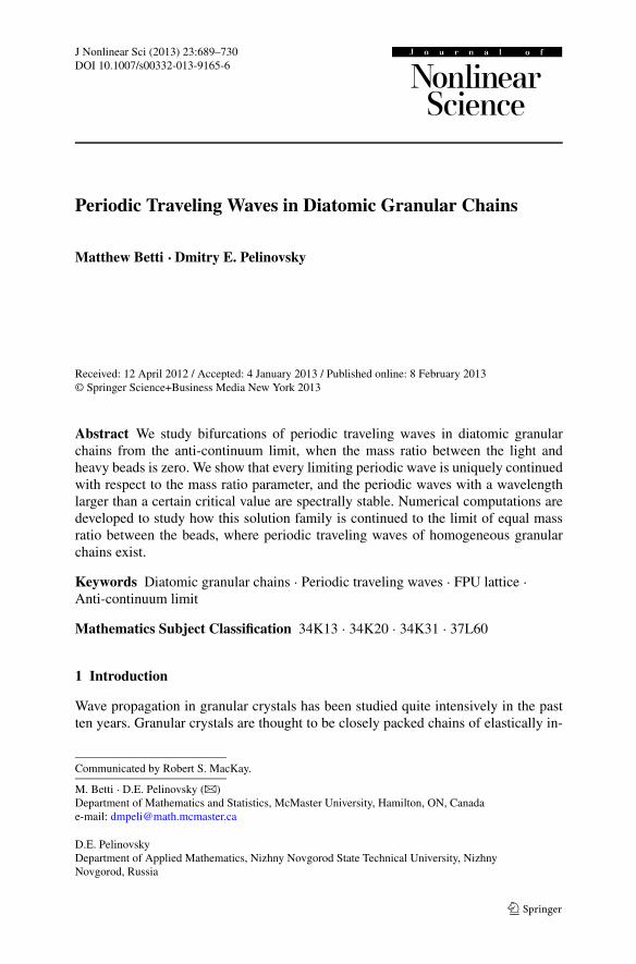
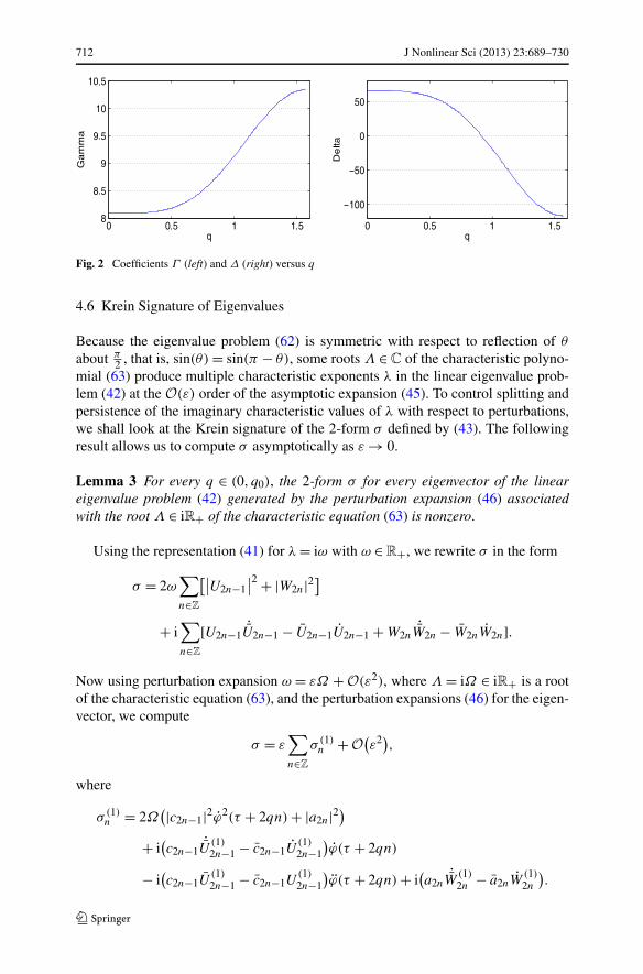
2 . The proof of Lemma 2 is complete.Numerical approximations of coefficients Γ and Δ versus q is shown on Fig. 2.
We can see from the figure that the sign change of Δ occurs at q0 ≈ 0.915.
712 J Nonlinear Sci (2013) 23:689–730
Fig. 2 Coefficients Γ (left) and Δ (right) versus q
4.6 Krein Signature of Eigenvalues
Because the eigenvalue problem (62) is symmetric with respect to reflection of θ
about π2 , that is, sin(θ) = sin(π − θ), some roots Λ ∈ C of the characteristic polyno-
mial (63) produce multiple characteristic exponents λ in the linear eigenvalue prob-lem (42) at the O(ε) order of the asymptotic expansion (45). To control splitting andpersistence of the imaginary characteristic values of λ with respect to perturbations,we shall look at the Krein signature of the 2-form σ defined by (43). The followingresult allows us to compute σ asymptotically as ε → 0.
Lemma 3 For every q ∈ (0, q0), the 2-form σ for every eigenvector of the lineareigenvalue problem (42) generated by the perturbation expansion (46) associatedwith the root Λ ∈ iR+ of the characteristic equation (63) is nonzero.
Using the representation (41) for λ = iω with ω ∈ R+, we rewrite σ in the form
σ = 2ω∑n∈Z
[∣∣U2n−1∣∣2 + |W2n|2
]
+ i∑n∈Z
[U2n−1˙U2n−1 − U2n−1U2n−1 + W2n
˙W2n − W2nW2n].
Now using perturbation expansion ω = εΩ + O(ε2), where Λ = iΩ ∈ iR+ is a rootof the characteristic equation (63), and the perturbation expansions (46) for the eigen-vector, we compute
σ = ε∑n∈Z
σ (1)n + O
(ε2),
where
σ (1)n = 2Ω
(|c2n−1|2ϕ2(τ + 2qn) + |a2n|2)
+ i(c2n−1
˙U(1)2n−1 − c2n−1U
(1)2n−1
)ϕ(τ + 2qn)
− i(c2n−1U
(1)2n−1 − c2n−1U
(1)2n−1
)ϕ(τ + 2qn) + i
(a2n
˙W(1)2n − a2nW
(1)2n
).
J Nonlinear Sci (2013) 23:689–730 713
Using representation (52), this becomes
σ (1)n = 2Ω
(|c2n−1|2E0 + |a2n|2) + i(c2n−1a2n − c2n−1a2n)E−
+ i(c2n−1a2n−2 − c2n−1a2n−2)E+,
where E0 and E± are τ -independent constants from the first integrals:
E0 = ϕ2 + ϕv − ϕv,
E± = ϕy± − ϕy± − z±.
Using explicit computations (56)–(60) of functions v, y±, and z±, we obtain
E0 = − 2π
T ′(E0), E± = ±2π − T ′(E0)(ϕ(0))2
πT ′(E0)ϕ(0),
and hence we have
σ (1)n = 2Ω
(K
2π|c2n−1|2 + |a2n|2
)
− iL2(c2n−1a2n − c2n−1a2n − c2n−1a2n−2 + c2n−1a2n−2).
Substituting the discrete Fourier transform representation (61) of the eigenvectorof the reduced eigenvalue problem (54), we obtain
σ (1)n = 2Ω
(K
2πC2 + A2
)− 4L2 sin(θ)CA
= 1
πΩ
(Ω2KC2 + 8πM2 sin2(θ)A2),
where the second equation of the linear system (62) has been used. Using now thefirst equation of the linear system (62), we obtain
σ (1)n = C2
πL1L2Ω3
[KL1L2Ω
4 + M2(KΩ2 − 4M1 sin2(θ)
)2]. (66)
Note that σ(1)n is independent of n, hence periodic boundary conditions are used to
obtain a finite expression for the 2-form σ .We consider q ∈ (0, q0) and θ ∈ (0,π), so that Ω = 0 and C = 0. Then, σ
(1)n = 0
if and only if
KL1L2Ω4 + M2
(KΩ2 − 4M1 sin2(θ)
)2 = 0.
Using the explicit expressions for coefficients (K,M1,M2,L1,L2) in Lemma 1, wefactorize the left hand side as follows:
KL1L2Ω4 + M2
(KΩ2 − 4M1 sin2(θ)
)2
= (Ω2 + T ′(E0)M1M2 sin2(θ)
)
714 J Nonlinear Sci (2013) 23:689–730
×(
32π2
(T ′(E0))2
(1 − T ′(E0)(ϕ(0))2
4π
)Ω2 + 16
T ′(E0)M1 sin2(θ)
). (67)
For every q ∈ (0, q0), M1 < 0, so that the second bracket is strictly positive (recallthat T ′(E0) < 0). Now the first bracket vanishes at
Ω2 = −2M1
π(ϕ(0))2sin2(θ).
Substituting this constraint to the characteristic equation (63) yields after straightfor-ward computations:
D(iΩ; θ) = 8M1 sin4(θ)
πϕ2(0)
(1 − 2π
T ′(E0)ϕ2(0)
)I (q),
which is nonzero for all q ∈ (0, q0) and θ ∈ (0,π). Therefore, σ(1)n does not vanish if
q ∈ (0, q0) and θ ∈ (0,π). By continuity of the perturbation expansions in ε, σ doesnot vanish too. The proof of Lemma 3 is complete.
Remark 9 For every q ∈ (0, q0), all roots Λ ∈ iR+ of the characteristic equation (63)are divided into two equal sets, one has σ
(1)n > 0 and the other one has σ
(1)n < 0. This
follows from the factorization
D(iΩ; θ) = − 4π2
T ′(E0)
(Ω2 − 4
π2sin2(θ)
)2
− 4I (q)
(Ω2 − 8
πT ′(E0)(ϕ(0))2sin2(θ)
)sin2(θ).
As q → 0, I (q) → 0 and perturbation theory for double roots (65) for q = 0 yields
Ω2 = 4
π2sin2(θ) ± 2
π2sin2(θ)
√∣∣T ′(E0)∣∣I (q)
(1 − 2π
T ′(E0)(ϕ(0))2
)+ O
(I (q)
).
Using the factorization formula (67), the sign of σ(1)n is determined by the expression
Ω2 + T ′(E0)M1M2 sin2(θ) = ± 2
π2sin2(θ)
√∣∣T ′(E0)∣∣I (q)
(1 − 2π
T ′(E0)(ϕ(0))2
)
+ O(I (q)
),
which justifies the claim for small positive q . By Lemma 3, σ(1)n does not vanish for
all q ∈ (0, q0) and θ ∈ (0,π), therefore the splitting of all roots Λ ∈ iR+ into twoequal sets persists for all values of q ∈ (0, q0).
J Nonlinear Sci (2013) 23:689–730 715
4.7 Proof of Theorem 2
To conclude the proof of Theorem 2, we develop rigorous perturbation theory in thecase when q = πm
Nfor some positive integers m and N such that 1 ≤ m ≤ N . In
this case, the linear eigenvalue problem (42) can be closed at 2mN second-orderdifferential equations subject to 2mN -periodic boundary conditions (15) and we arelooking for 4mN eigenvalues λ, which are characteristic exponents for a 4mN ×4mN Floquet matrix.
At ε = 0, we have 2mN double Jordan blocks for λ = 0. The 2mN eigenvectorsare given by (44). The 2mN -periodic boundary conditions are incorporated in thediscrete Fourier transform (61) if
θ = πk
mN≡ θk(m,N), k = 0,1, . . . ,mN − 1.
Because the characteristic equation (63) for each θk(m,N) returns 4 roots, we count4mN roots of the characteristic equation (63), as many as there are eigenvalues λ
in the linear eigenvalue problem (42) closed at 2mN second-order differential equa-tions. As long as the roots are non-degenerate (if Δ = Γ 2) and different from zero (ifΔ = 0), the first-order perturbation theory predicts splitting of λ = 0 into symmetricpairs of nonzero eigenvalues. The zero eigenvalue of multiplicity 4 persists and cor-responds to the value θ0(m,N) = 0. It is associated with the symmetries (7) and (8)of the diatomic granular chain.
The nonzero eigenvalues are located hierarchically with respect to the values ofsin2(θ) for θ = θk(m,N) with 1 ≤ k ≤ mN − 1. Because sin(θ) = sin(π − θ), everynonzero eigenvalue corresponding to θk(m,N) = π
2 is double. Because all eigenval-
ues λ ∈ iR+ have a definite Krein signature by Lemma 3 and the sign of σ(1)n in (66) is
same for both eigenvalues with θ and π − θ , the double eigenvalues λ ∈ iR are struc-turally stable with respect to parameter continuations (Chugunova and Pelinovsky2010) in the sense that they split along the imaginary axis beyond the leading-orderperturbation theory.
Remark 10 The argument based on the Krein signature cannot be applied to the caseof double real eigenvalues Λ ∈ R+, which may split off the real axis to the com-plex domain. However, both real and complex eigenvalues contribute to the count ofunstable eigenvalues with the account of their multiplicities.
It remains to address the issue that the perturbation theory in Sect. 4.3 uses com-putations of V ′′′, which is not a continuous function of its argument. To deal with thisissue, we use a renormalization technique. We note that if (u∗,w∗) is a solution of thedifferential advance–delay equations (14) given by Theorem 1, then differentiation ofthe first equation of the system yields
...u∗(τ ) = V ′′(w∗(τ ) − u∗(τ )
)(w∗(τ ) − u∗(τ )
)− V ′′(u∗(τ ) − w∗(τ − 2q)
)(u∗(τ ) − w∗(τ − 2q)
), (68)
where the right-hand side is a continuous function of τ .
716 J Nonlinear Sci (2013) 23:689–730
Using (68), we substitute
U2n−1 = c2n−1u∗(τ + 2qn) + U2n−1, W2n = W2n,
for an arbitrary choice of {c2n−1}n∈Z, into the linear eigenvalue problem (42) andobtain
⎧⎪⎪⎪⎪⎪⎪⎪⎪⎪⎪⎪⎪⎪⎪⎪⎪⎨⎪⎪⎪⎪⎪⎪⎪⎪⎪⎪⎪⎪⎪⎪⎪⎪⎩
U2n−1 + 2λU2n−1 + λ2 U2n−1= V ′′(w∗(τ + 2qn) − u∗(τ + 2qn))(εW2n − U2n−1)
− V ′′(u∗(τ + 2qn) − w∗(τ + 2qn − 2q))(U2n−1 − εW2n−2),
− (2λu∗(τ + 2qn) + λ2u∗(τ + 2qn))c2n−1− V ′′(w∗(τ + 2qn) − u∗(τ + 2qn))w∗(τ + 2qn)c2n−1− V ′′(u∗(τ + 2qn) − w∗(τ + 2qn − 2q))w∗(τ + 2qn − 2q)c2n−1,
W2n + 2λW2n + λ2 W2n
= εV ′′(u∗(τ + 2qn + 2q) − w∗(τ + 2qn))(U2n+1 − εW2n)
− εV ′′(w∗(τ + 2qn) − u∗(τ + 2qn))(εW2n − U2n−1)
+ εV ′′(u∗(τ + 2qn + 2q) − w∗(τ + 2qn))u∗(τ + 2qn + 2q)c2n−1+ εV ′′(w∗(τ + 2qn) − u∗(τ + 2qn))u∗(τ + 2qn)c2n−1.
(69)
When we repeat decompositions of the perturbation theory in Sect. 4.3, we write
λ = ελ(1) + ε2λ(2) + o(ε2),
U2n−1 = εU (1)2n−1 + ε2 U (2)
2n−1 + o(ε2),
W2n = a2n + εW (1)2n + ε2 W (2)
2n + o(ε2),
for an arbitrary choice of {a2n}n∈Z. Substituting this decomposition to system (69),we obtain equations at the O(ε) and O(ε2) orders, which do not require computationsof V ′′′. Hence, the system of difference equations (54) is justified at the O(ε2) orderand the splitting of the eigenvalues λ obeys roots of the characteristic equation (63).Persistence of roots beyond the O(ε2) order holds by the standard perturbation theoryfor isolated eigenvalues of the Floquet matrix. The proof of Theorem 2 is complete.
5 Numerical Results
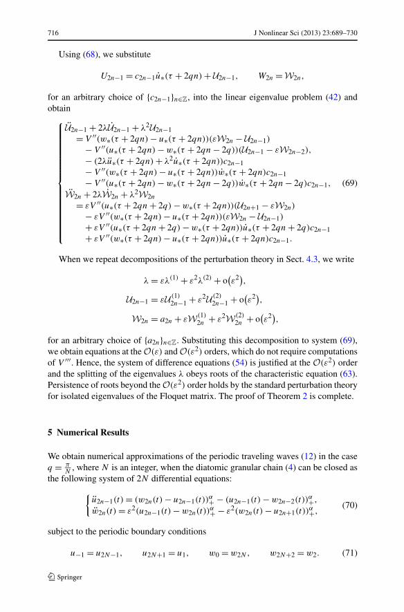
We obtain numerical approximations of the periodic traveling waves (12) in the caseq = π
N, where N is an integer, when the diatomic granular chain (4) can be closed as
the following system of 2N differential equations:
{u2n−1(t) = (w2n(t) − u2n−1(t))
α+ − (u2n−1(t) − w2n−2(t))α+,
w2n(t) = ε2(u2n−1(t) − w2n(t))α+ − ε2(w2n(t) − u2n+1(t))
α+,(70)
subject to the periodic boundary conditions
u−1 = u2N−1, u2N+1 = u1, w0 = w2N, w2N+2 = w2. (71)
J Nonlinear Sci (2013) 23:689–730 717
The periodic traveling waves (12) corresponds to 2π -periodic solutions of system(70) satisfying the reduction
u2n+1(t) = u2n−1
(t + 2π
N
), w2n+2(t) = w2n
(t + 2π
N
), (72)
For convenience and uniqueness, we look for an odd function u1(t) = −u1(−t) with
u1(0) = 0 and u1(0) > 0. (73)
By Theorem 1, the traveling wave solutions satisfying (72) and (73) are continueduniquely for small values of ε from the limiting solution with u1 = ϕ and w2 = 0.We continue numerically this branch of solutions with respect to parameter ε in theinterval [0,1].
5.1 Existence of Periodic Traveling Waves
In order to obtain 2π -periodic traveling wave solutions to the nonlinear system (70),we use the shooting method. Our shooting parameters are given by the initial condi-tions {
u2n−1(0), u2n−1(0),w2n(0), w2n(0)}
1≤n≤N.
Since u1(0) = 0, this gives a set of 2N − 1 shooting parameters. However, for so-lutions satisfying the traveling wave reduction (72), we can use symmetries of thenonlinear system of differential equations (70) to reduce the number of shooting pa-rameters to N parameters.
For two particles (N = 1 or q = π ), the existence and stability problems are trivial.The exact solution (23) is uniquely continued for all ε ∈ [0,1] and matches at ε =1 with the exact solution of the homogeneous granular chain considered in James(2012). This solution is spectrally stable with respect to 2-periodic perturbations forall ε ∈ [0,1] because the characteristic exponent λ = 0 has algebraic multiplicity four,which coincides with the total number of admissible characteristic values of λ in thelinearized system (38) closed at two second-order differential equations.
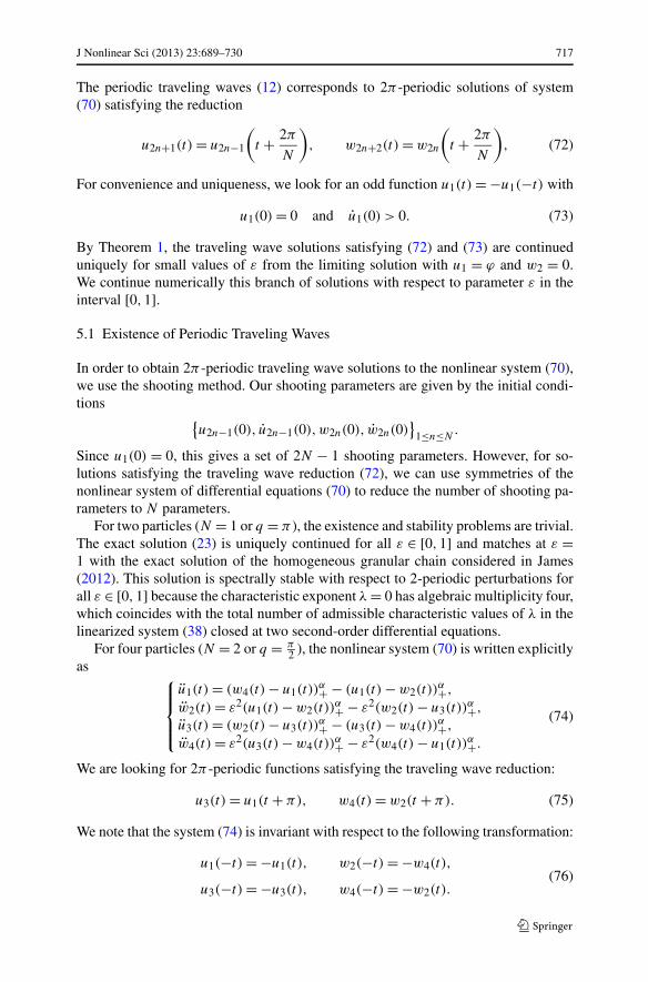
For four particles (N = 2 or q = π2 ), the nonlinear system (70) is written explicitly
as ⎧⎪⎪⎨⎪⎪⎩
u1(t) = (w4(t) − u1(t))α+ − (u1(t) − w2(t))
α+,
w2(t) = ε2(u1(t) − w2(t))α+ − ε2(w2(t) − u3(t))
α+,
u3(t) = (w2(t) − u3(t))α+ − (u3(t) − w4(t))
α+,
w4(t) = ε2(u3(t) − w4(t))α+ − ε2(w4(t) − u1(t))
α+.
(74)
We are looking for 2π -periodic functions satisfying the traveling wave reduction:
u3(t) = u1(t + π), w4(t) = w2(t + π). (75)
We note that the system (74) is invariant with respect to the following transformation:
u1(−t) = −u1(t), w2(−t) = −w4(t),
u3(−t) = −u3(t), w4(−t) = −w2(t).(76)
718 J Nonlinear Sci (2013) 23:689–730
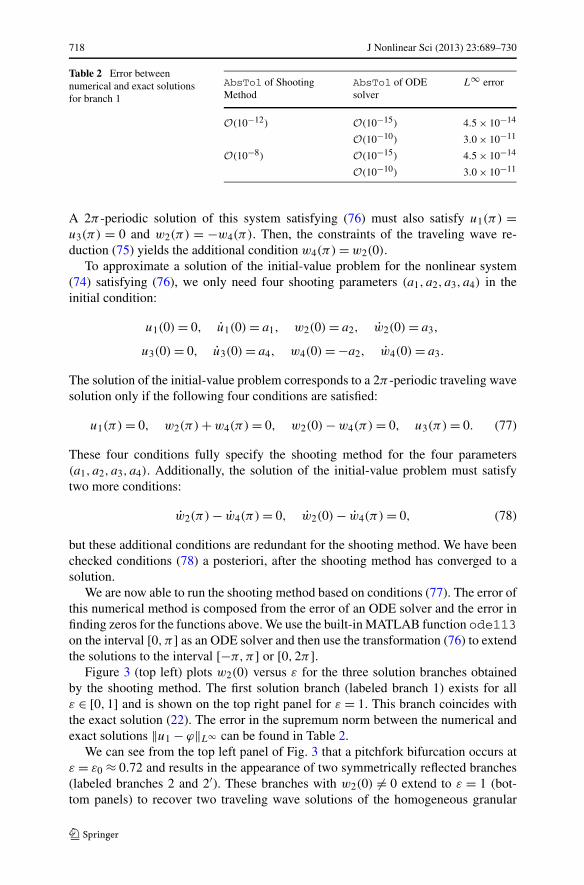
Table 2 Error betweennumerical and exact solutionsfor branch 1
AbsTol of ShootingMethod
AbsTol of ODEsolver
L∞ error
O(10−12) O(10−15) 4.5 × 10⁻¹⁴
O(10−10) 3.0 × 10⁻¹¹
O(10−8) O(10−15) 4.5 × 10⁻¹⁴
O(10−10) 3.0 × 10⁻¹¹
A 2π -periodic solution of this system satisfying (76) must also satisfy u1(π) =u3(π) = 0 and w2(π) = −w4(π). Then, the constraints of the traveling wave re-duction (75) yields the additional condition w4(π) = w2(0).
To approximate a solution of the initial-value problem for the nonlinear system(74) satisfying (76), we only need four shooting parameters (a1, a2, a3, a4) in theinitial condition:
u1(0) = 0, u1(0) = a1, w2(0) = a2, w2(0) = a3,
u3(0) = 0, u3(0) = a4, w4(0) = −a2, w4(0) = a3.
The solution of the initial-value problem corresponds to a 2π -periodic traveling wavesolution only if the following four conditions are satisfied:
u1(π) = 0, w2(π) + w4(π) = 0, w2(0) − w4(π) = 0, u3(π) = 0. (77)
These four conditions fully specify the shooting method for the four parameters(a1, a2, a3, a4). Additionally, the solution of the initial-value problem must satisfytwo more conditions:
w2(π) − w4(π) = 0, w2(0) − w4(π) = 0, (78)
but these additional conditions are redundant for the shooting method. We have beenchecked conditions (78) a posteriori, after the shooting method has converged to asolution.
We are now able to run the shooting method based on conditions (77). The error ofthis numerical method is composed from the error of an ODE solver and the error infinding zeros for the functions above. We use the built-in MATLAB function ode113on the interval [0,π] as an ODE solver and then use the transformation (76) to extendthe solutions to the interval [−π,π] or [0,2π].
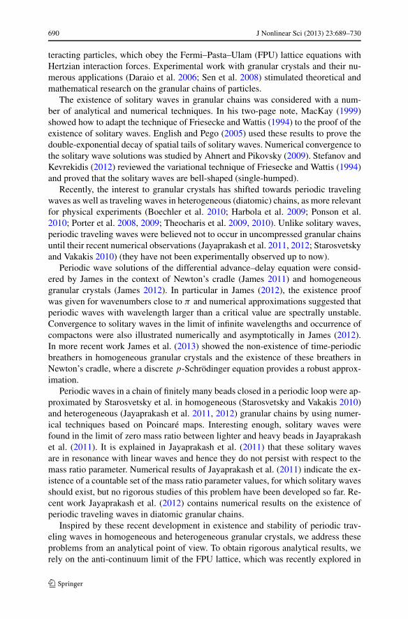
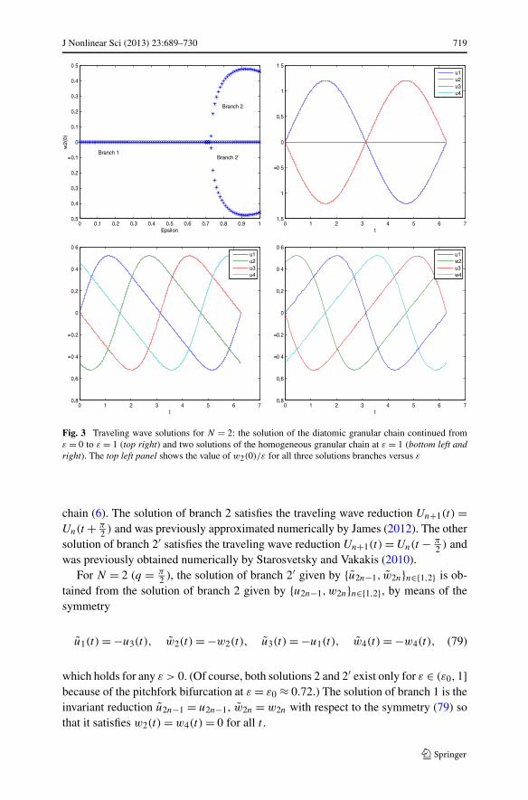
Figure 3 (top left) plots w2(0) versus ε for the three solution branches obtainedby the shooting method. The first solution branch (labeled branch 1) exists for allε ∈ [0,1] and is shown on the top right panel for ε = 1. This branch coincides withthe exact solution (22). The error in the supremum norm between the numerical andexact solutions ‖u1 − ϕ‖L∞ can be found in Table 2.
We can see from the top left panel of Fig. 3 that a pitchfork bifurcation occurs atε = ε0 ≈ 0.72 and results in the appearance of two symmetrically reflected branches(labeled branches 2 and 2′). These branches with w2(0) = 0 extend to ε = 1 (bot-tom panels) to recover two traveling wave solutions of the homogeneous granular
J Nonlinear Sci (2013) 23:689–730 719
Fig. 3 Traveling wave solutions for N = 2: the solution of the diatomic granular chain continued fromε = 0 to ε = 1 (top right) and two solutions of the homogeneous granular chain at ε = 1 (bottom left andright). The top left panel shows the value of w2(0)/ε for all three solutions branches versus ε
chain (6). The solution of branch 2 satisfies the traveling wave reduction Un+1(t) =Un(t + π
2 ) and was previously approximated numerically by James (2012). The othersolution of branch 2′ satisfies the traveling wave reduction Un+1(t) = Un(t − π
2 ) andwas previously obtained numerically by Starosvetsky and Vakakis (2010).
For N = 2 (q = π2 ), the solution of branch 2′ given by {u2n−1, w2n}n∈{1,2} is ob-
tained from the solution of branch 2 given by {u2n−1,w2n}n∈{1,2}, by means of thesymmetry
u1(t) = −u3(t), w2(t) = −w2(t), u3(t) = −u1(t), w4(t) = −w4(t), (79)
which holds for any ε > 0. (Of course, both solutions 2 and 2′ exist only for ε ∈ (ε0,1]because of the pitchfork bifurcation at ε = ε0 ≈ 0.72.) The solution of branch 1 is theinvariant reduction u2n−1 = u2n−1, w2n = w2n with respect to the symmetry (79) sothat it satisfies w2(t) = w4(t) = 0 for all t .
720 J Nonlinear Sci (2013) 23:689–730
For six particles (N = 3 or q = π3 ), the nonlinear system (70) is written explicitly
as ⎧⎪⎪⎪⎪⎪⎪⎨⎪⎪⎪⎪⎪⎪⎩
u1(t) = (w6(t) − u1(t))α+ − (u1(t) − w2(t))
α+,
w2(t) = ε2(u1(t) − w2(t))α+ − ε2(w2(t) − u3(t))
α+,
u3(t) = (w2(t) − u3(t))α+ − (u3(t) − w4(t))
α+,
w4(t) = ε2(u3(t) − w4(t))α+ − ε2(w4(t) − u5(t))
α+,
u5(t) = (w4(t) − u5(t))α+ − (u5(t) − w6(t))
α+,
w6(t) = ε2(u5(t) − w6(t))α+ − ε2(w6(t) − u1(t))
α+.
(80)
We are looking for 2π -periodic functions satisfying the traveling wave reduction:
u5(t) = u3
(t + 2π
3
)= u1
(t + 4π
3
),
w6(t) = w4
(t + 2π
3
)= w2
(t + 4π
3
).
(81)
We note that the system (80) is invariant with respect to the following transformation:
u1(−t) = −u1(t), w2(−t) = −w6(t),
u3(−t) = −u5(t), w4(−t) = −w4(t).(82)
A 2π -periodic solution of this system satisfying (82) must also satisfy u1(π) =w4(π) = 0, w2(π) = −w6(π), and u3(π) = −u5(π). Then, the constraints of thetraveling wave reduction (81) yield the conditions u3(π) = −u1(
π3 ) and w4(π) =
−w2(π3 ).
To approximate a solution of the initial-value problem for the nonlinear system(80) satisfying (82), we only need six shooting parameters (a1, a2, a3, a4, a5, a6) inthe initial condition:
u1(0) = 0, u1(0) = a1, w2(0) = a2, w2(0) = a3,
u3(0) = a4, u3(0) = a5, w4(0) = 0, w4(0) = a6,
u5(0) = −a4, u5(0) = a5, w6(0) = −a2, w6(0) = a3.
This solution corresponds to a 2π -periodic traveling wave solution only if it satisfiesthe following six conditions:
u1(π) = 0, w2(π) + w6(π) = 0, u3(π) + u5(π) = 0,
u1
(π
3
)+ u3(π) = 0, w2
(π
3
)+ w4(π) = 0, w4(π) = 0.
The six conditions determines the shooting method for the six parameters (a1, a2, a3,
a4, a5, a6). Additional conditions,
w2(π) − w6(π) = 0, u3(π) − u5(π) = 0,
u1
(π
3
)− u3(π) = 0, w2
(π
3
)− w4(π) = 0,
are to be checked a posteriori, after the shooting method has converged to a solution.
J Nonlinear Sci (2013) 23:689–730 721
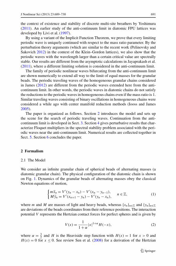
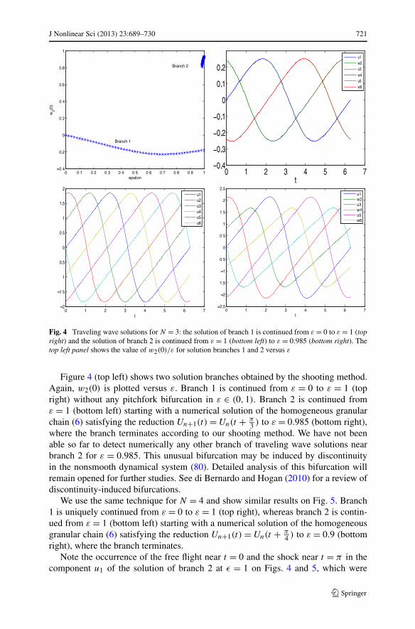
Fig. 4 Traveling wave solutions for N = 3: the solution of branch 1 is continued from ε = 0 to ε = 1 (topright) and the solution of branch 2 is continued from ε = 1 (bottom left) to ε = 0.985 (bottom right). Thetop left panel shows the value of w2(0)/ε for solution branches 1 and 2 versus ε
Figure 4 (top left) shows two solution branches obtained by the shooting method.Again, w2(0) is plotted versus ε. Branch 1 is continued from ε = 0 to ε = 1 (topright) without any pitchfork bifurcation in ε ∈ (0,1). Branch 2 is continued fromε = 1 (bottom left) starting with a numerical solution of the homogeneous granularchain (6) satisfying the reduction Un+1(t) = Un(t + π
3 ) to ε = 0.985 (bottom right),where the branch terminates according to our shooting method. We have not beenable so far to detect numerically any other branch of traveling wave solutions nearbranch 2 for ε = 0.985. This unusual bifurcation may be induced by discontinuityin the nonsmooth dynamical system (80). Detailed analysis of this bifurcation willremain opened for further studies. See di Bernardo and Hogan (2010) for a review ofdiscontinuity-induced bifurcations.
We use the same technique for N = 4 and show similar results on Fig. 5. Branch1 is uniquely continued from ε = 0 to ε = 1 (top right), whereas branch 2 is contin-ued from ε = 1 (bottom left) starting with a numerical solution of the homogeneousgranular chain (6) satisfying the reduction Un+1(t) = Un(t + π
4 ) to ε = 0.9 (bottomright), where the branch terminates.
Note the occurrence of the free flight near t = 0 and the shock near t = π in thecomponent u1 of the solution of branch 2 at ε = 1 on Figs. 4 and 5, which were
722 J Nonlinear Sci (2013) 23:689–730
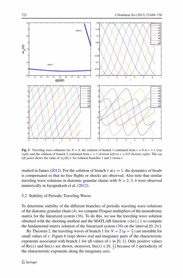
Fig. 5 Traveling wave solutions for N = 4: the solution of branch 1 continued from ε = 0 to ε = 1 (topright) and the solution of branch 2 continued from ε = 1 (bottom left) to ε = 0.9 (bottom right). The topleft panel shows the value of w2(0)/ε for solution branches 1 and 2 versus ε
studied in James (2012). For the solution of branch 1 at ε = 1, the dynamics of beadsis compensated so that no free flights or shocks are observed. Also note that similartraveling wave solutions in diatomic granular chains with N = 2,3,4 were observednumerically in Jayaprakash et al. (2012).
5.2 Stability of Periodic Traveling Waves
To determine stability of the different branches of periodic traveling wave solutionsof the diatomic granular chain (4), we compute Floquet multipliers of the monodromymatrix for the linearized system (36). To do this, we use the traveling wave solutionobtained with the shooting method and the MATLAB function ode113 to computethe fundamental matrix solution of the linearized system (36) on the interval [0,2π].
By Theorem 2, the traveling waves of branch 1 for N = 2 (q = π2 ) are unstable for
small values of ε. Figure 6 (top) shows real and imaginary parts of the characteristicexponents associated with branch 1 for all values of ε in [0,1]. Only positive valuesof Re(λ) and Im(λ) are shown, moreover, Im(λ) ∈ [0, 1
2 ] because of 1-periodicity ofthe characteristic exponents along the imaginary axis.
J Nonlinear Sci (2013) 23:689–730 723
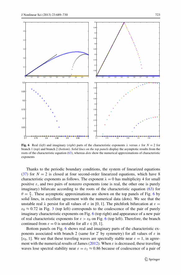
Fig. 6 Real (left) and imaginary (right) parts of the characteristic exponents λ versus ε for N = 2 forbranch 1 (top) and branch 2 (bottom). Solid lines on the top panels display the asymptotic results from theroots of the characteristic equation (63), whereas dots show the numerical approximations of characteristicexponents
Thanks to the periodic boundary conditions, the system of linearized equations(37) for N = 2 is closed at four second-order linearized equations, which have 8characteristic exponents as follows. The exponent λ = 0 has multiplicity 4 for smallpositive ε, and two pairs of nonzero exponents (one is real, the other one is purelyimaginary) bifurcate according to the roots of the characteristic equation (63) forθ = π
2 . These asymptotic approximations are shown on the top panels of Fig. 6 bysolid lines, in excellent agreement with the numerical data (dots). We see that theunstable real λ persist for all values of ε in [0,1]. The pitchfork bifurcation at ε =ε0 ≈ 0.72 in Fig. 3 (top left) corresponds to the coalescence of the pair of purelyimaginary characteristic exponents on Fig. 6 (top right) and appearance of a new pairof real characteristic exponents for ε > ε0 on Fig. 6 (top left). Therefore, the branchcontinued from ε = 0 is unstable for all ε ∈ [0,1].
Bottom panels on Fig. 6 shows real and imaginary parts of the characteristic ex-ponents associated with branch 2 (same for 2′ by symmetry) for all values of ε in[ε0,1]. We see that these traveling waves are spectrally stable near ε = 1, in agree-ment with the numerical results of James (2012). When ε is decreased, these travelingwaves lose spectral stability near ε = ε1 ≈ 0.86 because of coalescence of a pair of
724 J Nonlinear Sci (2013) 23:689–730
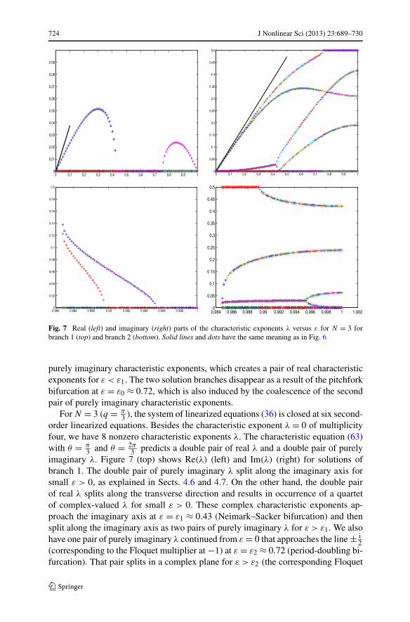
Fig. 7 Real (left) and imaginary (right) parts of the characteristic exponents λ versus ε for N = 3 forbranch 1 (top) and branch 2 (bottom). Solid lines and dots have the same meaning as in Fig. 6
purely imaginary characteristic exponents, which creates a pair of real characteristicexponents for ε < ε1. The two solution branches disappear as a result of the pitchforkbifurcation at ε = ε0 ≈ 0.72, which is also induced by the coalescence of the secondpair of purely imaginary characteristic exponents.
For N = 3 (q = π3 ), the system of linearized equations (36) is closed at six second-
order linearized equations. Besides the characteristic exponent λ = 0 of multiplicityfour, we have 8 nonzero characteristic exponents λ. The characteristic equation (63)with θ = π
3 and θ = 2π3 predicts a double pair of real λ and a double pair of purely
imaginary λ. Figure 7 (top) shows Re(λ) (left) and Im(λ) (right) for solutions ofbranch 1. The double pair of purely imaginary λ split along the imaginary axis forsmall ε > 0, as explained in Sects. 4.6 and 4.7. On the other hand, the double pairof real λ splits along the transverse direction and results in occurrence of a quartetof complex-valued λ for small ε > 0. These complex characteristic exponents ap-proach the imaginary axis at ε = ε1 ≈ 0.43 (Neimark–Sacker bifurcation) and thensplit along the imaginary axis as two pairs of purely imaginary λ for ε > ε1. We alsohave one pair of purely imaginary λ continued from ε = 0 that approaches the line ± i
2(corresponding to the Floquet multiplier at −1) at ε = ε2 ≈ 0.72 (period-doubling bi-furcation). That pair splits in a complex plane for ε > ε2 (the corresponding Floquet
J Nonlinear Sci (2013) 23:689–730 725
multipliers are real and negative). In summary, the periodic traveling wave of branch1 for N = 3 is stable for ε ∈ (ε1, ε2) but unstable near ε = 0 and ε = 1.
Figure 7 (bottom) shows Re(λ) (left) and Im(λ) (right) for solutions of branch 2that exist only for ε ∈ [ε∗,1], where ε∗ ≈ 0.985. All four pairs of the characteris-tic exponents λ are purely imaginary near ε = 1. This corresponds to the numericalresults for stability of traveling waves in the homogeneous granular chain in James(2012). Two pairs coalesce at ε ≈ 0.995 and split in a complex quartet of characteris-tic exponents (Neimark–Sacker bifurcation). Another pair approaches the line ± i
2 atε ≈ 0.989 and then splits in a complex plane to yield real and negative Floquet mul-tipliers (period-doubling bifurcation). The final remaining pair of purely imaginary λ
crosses zero near ε = ε∗ ≈ 0.985 that indicates that termination of branch 2 is relatedto a local (discontinuity-induced ?) bifurcation.
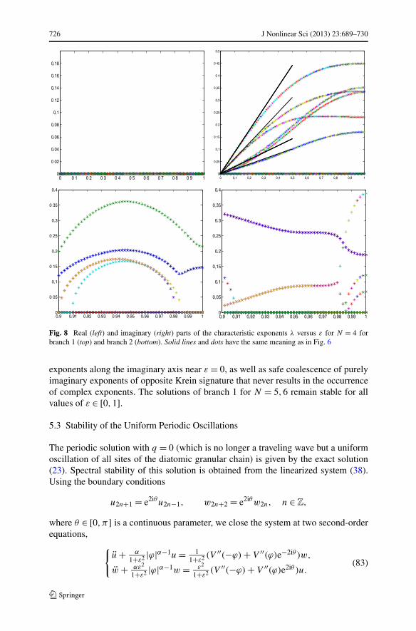
Recall that the coefficient M1 changes sign at q ≈ 0.915, as explained in Sect. 4.5.Therefore, for N ≥ 4, the characteristic equation (63) for any values of θ predictspairs of purely imaginary λ only. This is illustrated on the top panels of Fig. 8 forN = 4 (q = π
4 ). We can see that all double pairs of purely imaginary λ split alongthe imaginary axis for small ε > 0 and that the periodic traveling waves of branch1 remain stable for all ε ∈ [0,1]. The figure also illustrate the validity of asymptoticapproximations obtained from roots of the characteristic equation (63).
It is interesting that Fig. 8 (top right) shows safe coalescence of characteris-tic exponents for larger values of ε. Recall from Remark 9 that the character-istic exponents have opposite Krein signature for small values of ε in such away that larger exponents on Fig. 8 (top right) have negative Krein signature andsmaller exponents have positive Krein signature. It is typical to observe instabil-ities arise after the coalescence of two purely imaginary eigenvalues of the op-posite Krein signature (MacKay 1986) but this only happens when the doubleeigenvalue at the coalescence point is not semi-simple. When the double eigen-value is semi-simple or if some perturbation terms to the Jordan blocks are iden-tically zero, the coalescence does not introduce any instabilities (Bridges 1990;Vougalter and Pelinovsky 2006). This is precisely what we observe in Fig. 8 (topright). After coalescence, for larger values of ε, the purely imaginary characteristicexponents λ reappear as simple exponents with opposite Krein signature, that is, theexponents with positive Krein signature are now above the ones with negative Kreinsignature.
Figure 8 (bottom) shows Re(λ) (left) and Im(λ) (right) for solutions of branch 2that exist only for ε ∈ [ε∗,1], where ε∗ ≈ 0.90. Besides three pairs of purely imag-inary characteristic exponents λ, there is one pair of real λ and a complex quartetnear ε = 1. The pair of real λ corresponds to the numerical results for instability oftraveling waves in the homogeneous granular chain (James 2012), for which instabil-ity occurs for q � 0.9. The quartet of complex λ gives additional instability, whichis not captured by the reductions to the homogeneous granular chain. Several moreinstabilities arise as ε is decreased from ε = 1 for solutions of branch 2 because ofbifurcations of pairs of purely imaginary exponents λ. Branch 2 is unstable in theentire existence interval [ε∗,1].
Figure 9 shows the stability of solutions of branch 1 for N = 5 (left) and N = 6(right). These figures are included to illustrate the safe splitting of purely imaginary
726 J Nonlinear Sci (2013) 23:689–730
Fig. 8 Real (left) and imaginary (right) parts of the characteristic exponents λ versus ε for N = 4 forbranch 1 (top) and branch 2 (bottom). Solid lines and dots have the same meaning as in Fig. 6
exponents along the imaginary axis near ε = 0, as well as safe coalescence of purelyimaginary exponents of opposite Krein signature that never results in the occurrenceof complex exponents. The solutions of branch 1 for N = 5,6 remain stable for allvalues of ε ∈ [0,1].
5.3 Stability of the Uniform Periodic Oscillations
The periodic solution with q = 0 (which is no longer a traveling wave but a uniformoscillation of all sites of the diatomic granular chain) is given by the exact solution(23). Spectral stability of this solution is obtained from the linearized system (38).Using the boundary conditions
u2n+1 = e2iθu2n−1, w2n+2 = e2iθw2n, n ∈ Z,
where θ ∈ [0,π] is a continuous parameter, we close the system at two second-orderequations,
{u + α
1+ε2 |ϕ|α−1u = 11+ε2 (V ′′(−ϕ) + V ′′(ϕ)e−2iθ )w,
w + αε2
1+ε2 |ϕ|α−1w = ε2
1+ε2 (V ′′(−ϕ) + V ′′(ϕ)e2iθ )u.(83)
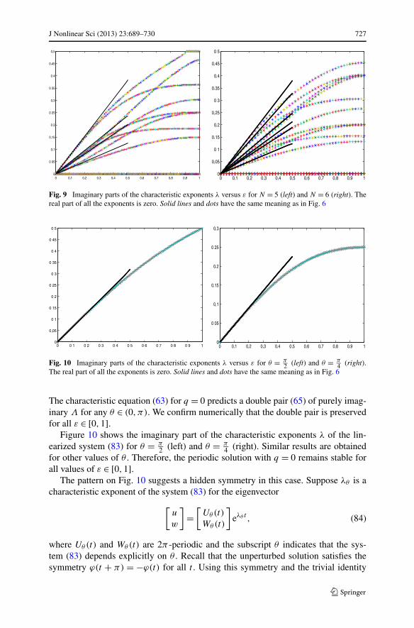
J Nonlinear Sci (2013) 23:689–730 727
Fig. 9 Imaginary parts of the characteristic exponents λ versus ε for N = 5 (left) and N = 6 (right). Thereal part of all the exponents is zero. Solid lines and dots have the same meaning as in Fig. 6
Fig. 10 Imaginary parts of the characteristic exponents λ versus ε for θ = π2 (left) and θ = π
4 (right).The real part of all the exponents is zero. Solid lines and dots have the same meaning as in Fig. 6
The characteristic equation (63) for q = 0 predicts a double pair (65) of purely imag-inary Λ for any θ ∈ (0,π). We confirm numerically that the double pair is preservedfor all ε ∈ [0,1].
Figure 10 shows the imaginary part of the characteristic exponents λ of the lin-earized system (83) for θ = π
2 (left) and θ = π4 (right). Similar results are obtained
for other values of θ . Therefore, the periodic solution with q = 0 remains stable forall values of ε ∈ [0,1].
The pattern on Fig. 10 suggests a hidden symmetry in this case. Suppose λθ is acharacteristic exponent of the system (83) for the eigenvector
[u
w
]=
[Uθ(t)
Wθ(t)
]eλθ t , (84)
where Uθ(t) and Wθ(t) are 2π -periodic and the subscript θ indicates that the sys-tem (83) depends explicitly on θ . Recall that the unperturbed solution satisfies thesymmetry ϕ(t + π) = −ϕ(t) for all t . Using this symmetry and the trivial identity
728 J Nonlinear Sci (2013) 23:689–730
e2π i = 1, we can verify that there is another solution of the system (83) with the sameθ for the characteristic exponent λπ−θ :
[u
w
]=
[Uπ−θ (t + π)
e2iθWπ−θ (t + π)
]eλπ−θ t . (85)
From the symmetry of roots (65) and the corresponding characteristic exponents, wehave λθ = λπ−θ . The eigenvectors (84) and (85) are generally linearly independentand coexist for the same value of λ = λθ = λπ−θ . This argument explains the doubledegeneracy of characteristic exponents λ for the case q = 0 for all values of ε ∈ [0,1].
6 Conclusion
We have studied periodic traveling waves in a diatomic granular chain by continuingthese solutions from the anti-continuum limit, when the mass ratio between the lightand heavy beads is zero. We have shown that every limiting periodic wave is uniquelycontinued for small mass ratios. Although the vector fields of the granular dimer chainequations are not C2 at the origin, we can still use the implicit function theorem toguarantee that the continuation is C1 with respect to the mass ratio parameter ε2.We have also used rigorous perturbation theory to compute characteristic exponentsin the linearized stability problem. From this theory, we have seen that the periodicwaves with a wavelength larger than a certain critical value are spectrally stable forsmall mass ratios.
Numerical computations are developed to show that the stability of these periodicwaves with larger wavelengths extends all way to the limit of equal mass ratio. On theother hand, we have also computed periodic traveling waves that are continued fromsolutions of the homogeneous granular chain at the equal mass ratio, their spectralstability, and their terminations for smaller mass ratios.
Among open problems, we have not clarified the nature of bifurcation, where thesolutions of branch 2 terminate at a ε∗ ∈ (0,1) for N = 3,4. We have not been able tofind another solution for ε near ε∗. Safe coalescence of purely imaginary character-istic exponents λ of opposite Krein signatures is also amazing and we have not beenable to find the hidden symmetry that would explain why the eigenvalues of oppositeKrein signatures remain stable past the coalescence point. These problems as well asanalysis of the periodic traveling wave solutions for other values of q will wait forfurther studies.
Finally, our paper may inspire further experimental work with diatomic granu-lar crystals. We hope that some stable configurations of periodic traveling waves ina periodic granular chain of finitely many beads produced in our studies might befound experimentally to play important role in the dynamics of uncompressed gran-ular crystals.
Acknowledgements The research of the authors was supported by funding from the NSERC Discoverygrant and the Ministry of Education and Science of Russian Federation (project 14.B37.21.0868). Theauthors thank G. James, P. Kevrekidis, and Y. Starosvetsky for useful discussions.
J Nonlinear Sci (2013) 23:689–730 729
References
Ahnert, K., Pikovsky, A.: Compactons and chaos in strongly nonlinear lattices. Phys. Rev. E 79, 026209(2009)
Aubry, S.: Breathers in nonlinear lattices: Existence, linear stability and quantization. Physica D 103,201–250 (1997)
Boechler, N., Theocharis, G., Job, S., Kevrekidis, P.G., Porter, M.A., Daraio, C.: Discrete breathers inone-dimensional diatomic granular crystals. Phys. Rev. Lett. 104, 244302 (2010)
Bridges, T.J.: Bifurcation of periodic solutions near a collision of eigenvalues of opposite signature. Math.Proc. Camb. Philos. Soc. 108, 575–601 (1990)
Chugunova, M., Pelinovsky, D.: On quadratic eigenvalue problems arising in stability of discrete vortices.Linear Algebra Appl. 431, 962–973 (2009)
Chugunova, M., Pelinovsky, D.: Count of unstable eigenvalues in the generalized eigenvalue problem.J. Math. Phys. 51, 052901 (2010)
Daraio, C., Nesterenko, V.F., Herbold, E.B., Jin, S.: Tunability of solitary wave properties in one-dimensional strongly nonlinear phononic crystals. Phys. Rev. E 73, 026610 (2006)
di Bernardo, M., Hogan, S.J.: Discontinuity-induced bifurcations of piecewise smooth dynamical systems.Philos. Trans. R. Soc., Math. Phys. Eng. Sci. 368, 4915–4935 (2010)
English, J.M., Pego, R.L.: On the solitary wave pulse in a chain of beads. Proc. Am. Math. Soc. 133,1763–1768 (2005)
Friesecke, G., Wattis, J.A.D.: Existence theorem for solitary waves on lattices. Commun. Math. Phys. 161,391–418 (1994)
Harbola, U., Rosas, A., Romero, A.H., Esposito, M., Lindenberg, K.: Pulse propagation in decorated gran-ular chains: an analytical approach. Phys. Rev. E 80, 051302 (2009)
Iooss, G., James, G.: Localized waves in nonlinear oscillator chains. Chaos 15, 015113 (2005)James, G.: Nonlinear waves in Newton’s cradle and the discrete p-Schrödinger equation. Math. Models
Methods Appl. Sci. 21, 2335–2377 (2011)James, G.: Periodic travelling waves and compactons in granular chains. J. Nonlinear Sci. 22, 813–848
(2012)James, G., Kevrekidis, P.G., Cuevas, J.: Breathers in oscillatory chains with Hertzian interactions. Physica
D (2013, in press)Jayaprakash, K.R., Starosvetsky, Yu., Vakakis, A.F.: New family of solitary waves in granular dimer chains
with no precompression. Phys. Rev. E 83, 036606 (2011)Jayaprakash, K.R., Vakakis, A.F., Starosvetsky, Yu.: Strongly nonlinear traveling waves in granular dimer
chains. Mech. Syst. Signal Process. (2012). doi:10.1016/j.ymssp.2012.04.018Kapitula, T., Kevrekidis, P.G., Sandstede, B.: Counting eigenvalues via the Krein signature in infinite-
dimensional Hamiltonian systems. Physica D 195, 263–282 (2004). Addendum: Physica D 201, 199–201 (2005)
Kollar, R.: Homotopy method for nonlinear eigenvalue pencils with applications. SIAM J. Math. Anal. 43,612–633 (2011)
Livi, R., Spicci, M., MacKay, R.S.: Breathers on a diatomic FPU chain. Nonlinearity 10, 1421–1434(1997)
MacKay, R.S.: Stability of equilibria of Hamiltonian systems. In: Nonlinear Phenomenon and Chaos.Malvern Phys. Ser., pp. 254–270. Hilger, Bristol (1986)
MacKay, R.S.: Solitary waves in a chain of beads under Hertz contact. Phys. Lett. A 251, 191–192 (1999)Pelinovsky, D.E.: Inertia law for spectral stability of solitary waves in coupled nonlinear Schrödinger
equations. Proc. R. Soc. Lond. A 461, 783–812 (2005)Pelinovsky, D.E., Sakovich, A.: Multi-site breathers in Klein–Gordon lattices: stability, resonances, and
bifurcations. Nonlinearity 25, 3423–3451 (2012)Ponson, L., Boechler, N., Lai, Y.M., Porter, M.A., Kevrekidis, P.G., Daraio, C.: Nonlinear waves in disor-
dered diatomic granular chains. Phys. Rev. E 82, 021301 (2010)Porter, M.A., Daraio, C., Herbold, E.B., Szelengowicz, I., Kevrekidis, P.G.: Highly nonlinear solitary
waves in periodic dimer granular chains. Phys. Rev. E 77, 015601(R) (2008)Porter, M.A., Daraio, C., Szelengowics, I., Herbold, E.B., Kevrekidis, P.G.: Highly nonlinear solitary
waves in heterogeneous periodic granular media. Physica D 238, 666–676 (2009)Sen, S., Hong, J., Bang, J., Avalos, E., Doney, R.: Solitary waves in the granular chain. Phys. Rep. 462,
21–66 (2008)Starosvetsky, Yu., Vakakis, A.F.: Traveling waves and localized modes in one-dimensional homogeneous
granular chains with no precompression. Phys. Rev. E 82, 026603 (2010)
730 J Nonlinear Sci (2013) 23:689–730
Stefanov, A., Kevrekidis, P.G.: On the existence of solitary traveling waves for generalized Hertzian chains.J. Nonlinear Sci. 22, 327–349 (2012)
Theocharis, G., Kavousanakis, M., Kevrekidis, P.G., Daraio, C., Porter, M.A., Kevrekidis, I.G.: Localizedbreathing modes in granular crystals with defects. Phys. Rev. E 80, 066601 (2009)
Theocharis, G., Boechler, N., Kevrekidis, P.G., Job, S., Porter, M.A., Daraio, C.: Intrinsic energy localiza-tion through discrete gap breathers in one-dimensional diatomic granular crystals. Phys. Rev. E 82,056604 (2010)
Vougalter, V., Pelinovsky, D.: Eigenvalues of zero energy in the linearized NLS problem. J. Math. Phys.47, 062701 (2006)
Yoshimura, K.: Existence and stability of discrete breathers in diatomic Fermi–Pasta–Ulam type lattices.Nonlinearity 24, 293–317 (2011)

![Flavour Symmetries in Pati-Salam Grand Unifying Theories · GUT we limit ourselves to the Pati-Salam symmetry (PS) [6, 7]. The PS symmetry itself does The PS symmetry itself does](https://img.pdfslide.us/doc/110x75/5cab0dab88c993123c8c8b1d/flavour-symmetries-in-pati-salam-grand-unifying-theories-gut-we-limit-ourselves.jpg)