Performing Vacuum Calculations Using ANSYS

Kris A. Anderson

Performing Vacuum Calculations Using ANSYS

ANSYS does not have a module for performing vacuum calculations, but it does have a module

for performing thermal calculations. Using analogies, we can set up a heat flow problem such

that the solution is exactly the same as the solution for our desired vacuum problem. This paper

will show how that is done.

Vacuum

Pictured above is a vacuum element. There are two nodes, I and J, which comprise the

beginning and end of the element, respectively. Let’s assume that this element represents a

tube in a vacuum system, and thus that it outgasses from its interior surfaces at some rate. A

list of element attributes and environmental parameters follows.

Length: L (m) [Commonly listed in cm]

Perimeter: Ω (m) [Commonly listed in cm]

Cross Sectional Area: Across (m2) [Commonly listed in cm2]

Surface Area: Asurface (m2) [Commonly listed in cm2]

Conductance: C (m3/s) [Commonly listed in L/s]

Specific Outgassing Rate: Qoutgas (Pa·m/s) [Commonly listed in Torr·L/s·cm2]

Pressure: P (Pa) [Commonly listed in Torr]

Molecular Flow Rate: Q (Pa·m3/s) [Commonly listed in Torr·L/s]

The equation describing molecular flow in high vacuum is:

𝑄 = 𝐶∆𝑃

Most of the time these vacuum parameters will use the units of Torr, Liters, centimeters, and so

on. The first step to using ANSYS for this analysis should be to convert all of these units to the

ones listed above, which use Pascals, cubic meters, meters, etc. Some of the pertinent

conversions are listed below.

1 L = 0.001 m3

1 Torr = 133.322368 Pa

1 Torr·L/s·cm2 = 1333.22368 Pa·m/s

1 Torr·L/s = 0.133322368 Pa·m3/s

I J

Heat Transfer

Pictured above is a thermal element. There are two nodes, I and J, which comprise the

beginning and end of the element, respectively. Let’s assume that this element represents a

solid rod in a thermal system, and that it has internal heat generation occurring at some rate. A

list of element attributes and environmental parameters follows.

Length: L (m)

Cross Sectional Area: Across (m2)

Thermal Conductivity: k (W/m·K)

Volumetric Heat Generation Rate: q̇ (W/m3)

Temperature: T (K)

Heat Flow Rate: q (W)

The equation describing heat flow is:

𝑞 =𝑘𝐴∆𝑇

𝐿

Analogues

As previously stated, the two important equations are:

𝑄 = 𝐶∆𝑃

𝑞 = (𝑘𝐴

𝐿) ∆𝑇

Writing the equations in this format, it is apparent that:

Heat flow rate (q) is equivalent to molecular flow rate (Q).

The quantity (𝑘𝐴

𝐿) is equivalent to conductance (C).

Temperature (T) is equivalent to pressure (P).

These equivalencies are the key to formulating a thermal problem using our vacuum problem.

ANSYS wants thermal elements with properties like L, Across, k, and q̇. It also wants any

environmental constraints such as constrained nodal temperatures or heat flow rates. Our

vacuum problem will have vacuum elements with properties like L, Ω, Across, Asurface, C, and

Qoutgas. We also may have environmental constraints such as constrained nodal pressures or gas

I J

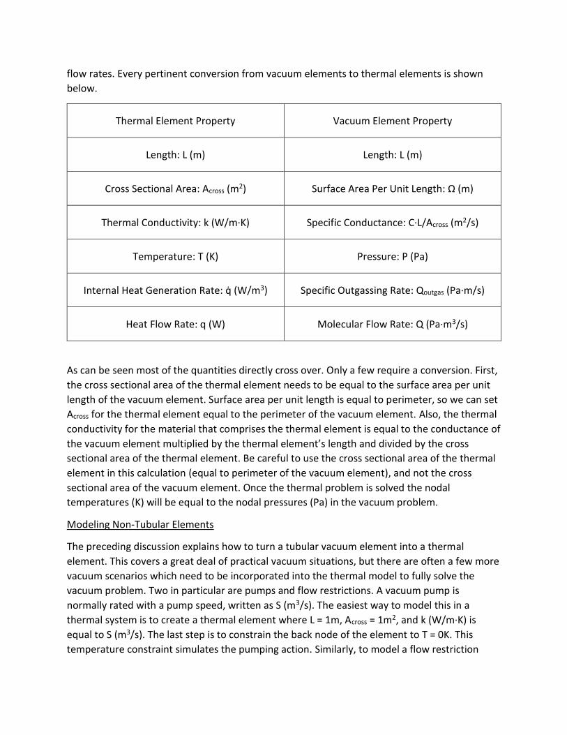
flow rates. Every pertinent conversion from vacuum elements to thermal elements is shown

below.

Thermal Element Property Vacuum Element Property

Length: L (m) Length: L (m)

Cross Sectional Area: Across (m2) Surface Area Per Unit Length: Ω (m)

Thermal Conductivity: k (W/m·K) Specific Conductance: C·L/Across (m2/s)

Temperature: T (K) Pressure: P (Pa)

Internal Heat Generation Rate: q̇ (W/m3) Specific Outgassing Rate: Qoutgas (Pa·m/s)

Heat Flow Rate: q (W) Molecular Flow Rate: Q (Pa·m3/s)

As can be seen most of the quantities directly cross over. Only a few require a conversion. First,

the cross sectional area of the thermal element needs to be equal to the surface area per unit

length of the vacuum element. Surface area per unit length is equal to perimeter, so we can set

Across for the thermal element equal to the perimeter of the vacuum element. Also, the thermal

conductivity for the material that comprises the thermal element is equal to the conductance of

the vacuum element multiplied by the thermal element’s length and divided by the cross

sectional area of the thermal element. Be careful to use the cross sectional area of the thermal

element in this calculation (equal to perimeter of the vacuum element), and not the cross

sectional area of the vacuum element. Once the thermal problem is solved the nodal

temperatures (K) will be equal to the nodal pressures (Pa) in the vacuum problem.

Modeling Non-Tubular Elements

The preceding discussion explains how to turn a tubular vacuum element into a thermal

element. This covers a great deal of practical vacuum situations, but there are often a few more

vacuum scenarios which need to be incorporated into the thermal model to fully solve the

vacuum problem. Two in particular are pumps and flow restrictions. A vacuum pump is

normally rated with a pump speed, written as S (m3/s). The easiest way to model this in a

thermal system is to create a thermal element where L = 1m, Across = 1m2, and k (W/m·K) is

equal to S (m3/s). The last step is to constrain the back node of the element to T = 0K. This

temperature constraint simulates the pumping action. Similarly, to model a flow restriction

with a conductance C (m3/s), create a thermal element where L = 1m, Across = 1m2, and k

(W/m·K) is equal to C (m3/s).

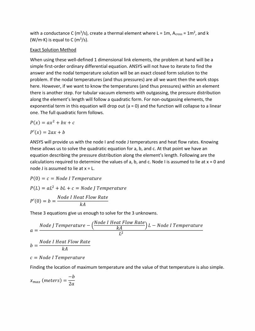
Exact Solution Method

When using these well-defined 1 dimensional link elements, the problem at hand will be a

simple first-order ordinary differential equation. ANSYS will not have to iterate to find the

answer and the nodal temperature solution will be an exact closed form solution to the

problem. If the nodal temperatures (and thus pressures) are all we want then the work stops

here. However, if we want to know the temperatures (and thus pressures) within an element

there is another step. For tubular vacuum elements with outgassing, the pressure distribution

along the element’s length will follow a quadratic form. For non-outgassing elements, the

exponential term in this equation will drop out (a = 0) and the function will collapse to a linear

one. The full quadratic form follows.

𝑃(𝑥) = 𝑎𝑥2 + 𝑏𝑥 + 𝑐

𝑃′(𝑥) = 2𝑎𝑥 + 𝑏

ANSYS will provide us with the node I and node J temperatures and heat flow rates. Knowing

these allows us to solve the quadratic equation for a, b, and c. At that point we have an

equation describing the pressure distribution along the element’s length. Following are the

calculations required to determine the values of a, b, and c. Node I is assumed to lie at x = 0 and

node J is assumed to lie at x = L.

𝑃(0) = 𝑐 = 𝑁𝑜𝑑𝑒 𝐼 𝑇𝑒𝑚𝑝𝑒𝑟𝑎𝑡𝑢𝑟𝑒

𝑃(𝐿) = 𝑎𝐿2 + 𝑏𝐿 + 𝑐 = 𝑁𝑜𝑑𝑒 𝐽 𝑇𝑒𝑚𝑝𝑒𝑟𝑎𝑡𝑢𝑟𝑒

𝑃′(0) = 𝑏 =𝑁𝑜𝑑𝑒 𝐼 𝐻𝑒𝑎𝑡 𝐹𝑙𝑜𝑤 𝑅𝑎𝑡𝑒

𝑘𝐴

These 3 equations give us enough to solve for the 3 unknowns.

𝑎 =𝑁𝑜𝑑𝑒 𝐽 𝑇𝑒𝑚𝑝𝑒𝑟𝑎𝑡𝑢𝑟𝑒 − (

𝑁𝑜𝑑𝑒 𝐼 𝐻𝑒𝑎𝑡 𝐹𝑙𝑜𝑤 𝑅𝑎𝑡𝑒𝑘𝐴

) 𝐿 − 𝑁𝑜𝑑𝑒 𝐼 𝑇𝑒𝑚𝑝𝑒𝑟𝑎𝑡𝑢𝑟𝑒

𝐿2

𝑏 =𝑁𝑜𝑑𝑒 𝐼 𝐻𝑒𝑎𝑡 𝐹𝑙𝑜𝑤 𝑅𝑎𝑡𝑒

𝑘𝐴

𝑐 = 𝑁𝑜𝑑𝑒 𝐼 𝑇𝑒𝑚𝑝𝑒𝑟𝑎𝑡𝑢𝑟𝑒

Finding the location of maximum temperature and the value of that temperature is also simple.

𝑥𝑚𝑎𝑥 (𝑚𝑒𝑡𝑒𝑟𝑠) =−𝑏

2𝑎

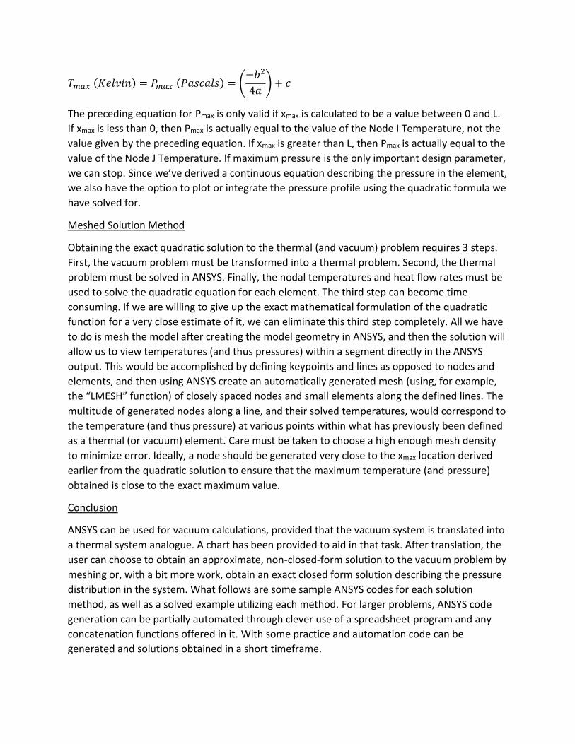
𝑇𝑚𝑎𝑥 (𝐾𝑒𝑙𝑣𝑖𝑛) = 𝑃𝑚𝑎𝑥 (𝑃𝑎𝑠𝑐𝑎𝑙𝑠) = (−𝑏2

4𝑎) + 𝑐

The preceding equation for Pmax is only valid if xmax is calculated to be a value between 0 and L.

If xmax is less than 0, then Pmax is actually equal to the value of the Node I Temperature, not the

value given by the preceding equation. If xmax is greater than L, then Pmax is actually equal to the

value of the Node J Temperature. If maximum pressure is the only important design parameter,

we can stop. Since we’ve derived a continuous equation describing the pressure in the element,

we also have the option to plot or integrate the pressure profile using the quadratic formula we

have solved for.

Meshed Solution Method

Obtaining the exact quadratic solution to the thermal (and vacuum) problem requires 3 steps.

First, the vacuum problem must be transformed into a thermal problem. Second, the thermal

problem must be solved in ANSYS. Finally, the nodal temperatures and heat flow rates must be

used to solve the quadratic equation for each element. The third step can become time

consuming. If we are willing to give up the exact mathematical formulation of the quadratic

function for a very close estimate of it, we can eliminate this third step completely. All we have

to do is mesh the model after creating the model geometry in ANSYS, and then the solution will

allow us to view temperatures (and thus pressures) within a segment directly in the ANSYS

output. This would be accomplished by defining keypoints and lines as opposed to nodes and

elements, and then using ANSYS create an automatically generated mesh (using, for example,

the “LMESH” function) of closely spaced nodes and small elements along the defined lines. The

multitude of generated nodes along a line, and their solved temperatures, would correspond to

the temperature (and thus pressure) at various points within what has previously been defined

as a thermal (or vacuum) element. Care must be taken to choose a high enough mesh density

to minimize error. Ideally, a node should be generated very close to the xmax location derived

earlier from the quadratic solution to ensure that the maximum temperature (and pressure)

obtained is close to the exact maximum value.

Conclusion

ANSYS can be used for vacuum calculations, provided that the vacuum system is translated into

a thermal system analogue. A chart has been provided to aid in that task. After translation, the

user can choose to obtain an approximate, non-closed-form solution to the vacuum problem by

meshing or, with a bit more work, obtain an exact closed form solution describing the pressure

distribution in the system. What follows are some sample ANSYS codes for each solution

method, as well as a solved example utilizing each method. For larger problems, ANSYS code

generation can be partially automated through clever use of a spreadsheet program and any

concatenation functions offered in it. With some practice and automation code can be

generated and solutions obtained in a short timeframe.

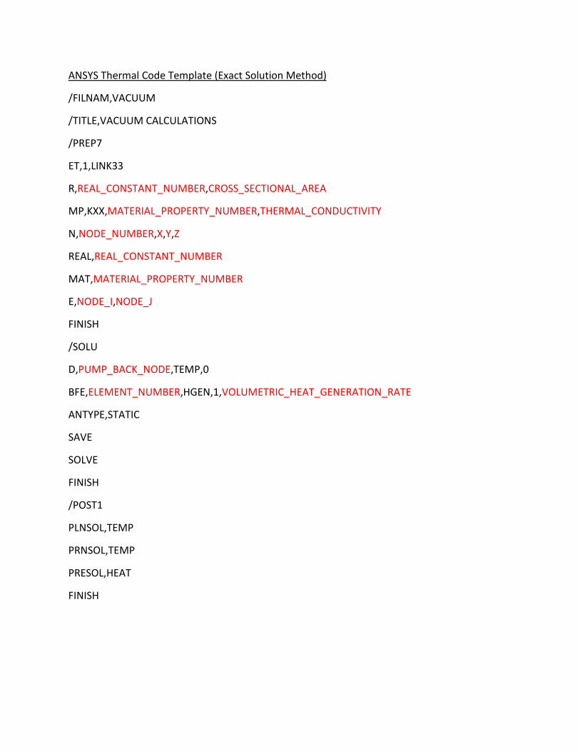
ANSYS Thermal Code Template (Exact Solution Method)

/FILNAM,VACUUM

/TITLE,VACUUM CALCULATIONS

/PREP7

ET,1,LINK33

R,REAL_CONSTANT_NUMBER,CROSS_SECTIONAL_AREA

MP,KXX,MATERIAL_PROPERTY_NUMBER,THERMAL_CONDUCTIVITY

N,NODE_NUMBER,X,Y,Z

REAL,REAL_CONSTANT_NUMBER

MAT,MATERIAL_PROPERTY_NUMBER

E,NODE_I,NODE_J

FINISH

/SOLU

D,PUMP_BACK_NODE,TEMP,0

BFE,ELEMENT_NUMBER,HGEN,1,VOLUMETRIC_HEAT_GENERATION_RATE

ANTYPE,STATIC

SAVE

SOLVE

FINISH

/POST1

PLNSOL,TEMP

PRNSOL,TEMP

PRESOL,HEAT

FINISH

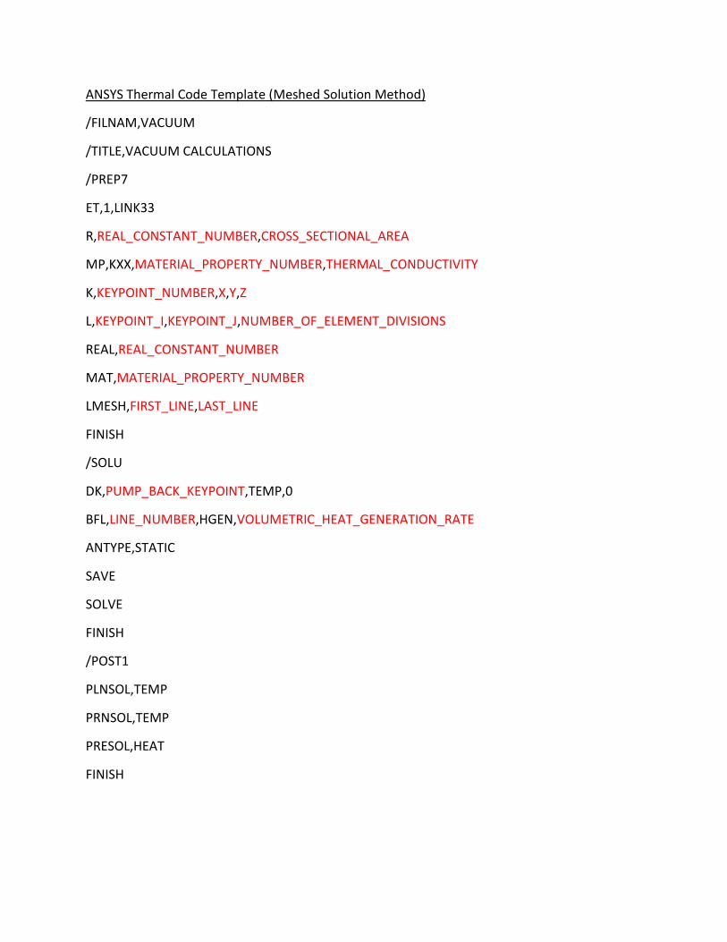
ANSYS Thermal Code Template (Meshed Solution Method)

/FILNAM,VACUUM

/TITLE,VACUUM CALCULATIONS

/PREP7

ET,1,LINK33

R,REAL_CONSTANT_NUMBER,CROSS_SECTIONAL_AREA

MP,KXX,MATERIAL_PROPERTY_NUMBER,THERMAL_CONDUCTIVITY

K,KEYPOINT_NUMBER,X,Y,Z

L,KEYPOINT_I,KEYPOINT_J,NUMBER_OF_ELEMENT_DIVISIONS

REAL,REAL_CONSTANT_NUMBER

MAT,MATERIAL_PROPERTY_NUMBER

LMESH,FIRST_LINE,LAST_LINE

FINISH

/SOLU

DK,PUMP_BACK_KEYPOINT,TEMP,0

BFL,LINE_NUMBER,HGEN,VOLUMETRIC_HEAT_GENERATION_RATE

ANTYPE,STATIC

SAVE

SOLVE

FINISH

/POST1

PLNSOL,TEMP

PRNSOL,TEMP

PRESOL,HEAT

FINISH

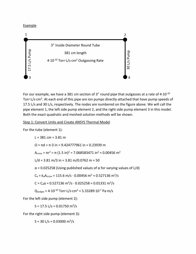
Example

For our example, we have a 381 cm section of 3” round pipe that outgasses at a rate of 4·10-10

Torr·L/s·cm2. At each end of this pipe are ion pumps directly attached that have pump speeds of

17.5 L/s and 30 L/s, respectively. The nodes are numbered on the figure above. We will call the

pipe element 1, the left side pump element 2, and the right side pump element 3 in this model.

Both the exact quadratic and meshed solution methods will be shown.

Step 1: Convert Units and Create ANSYS Thermal Model

For the tube (element 1):

L = 381 cm = 3.81 m

Ω = πd = π·3 in = 9.424777961 in ≈ 0.23939 m

Across = πr2 = π·(1.5 in)2 = 7.068583471 in2 ≈ 0.00456 m2

L/d = 3.81 m/3 in = 3.81 m/0.0762 m = 50

α = 0.025258 (Using published values of α for varying values of L/d)

Ca = kaAcross = 115.6 m/s · 0.00456 m2 ≈ 0.527136 m3/s

C = Caα = 0.527136 m3/s · 0.025258 ≈ 0.01331 m3/s

Qoutgas = 4·10-10 Torr·L/s·cm2 ≈ 5.33289·10-7 Pa·m/s

For the left side pump (element 2):

S = 17.5 L/s = 0.01750 m3/s

For the right side pump (element 3):

S = 30 L/s = 0.03000 m3/s

3

3” Inside Diameter Round Tube

381 cm length

4·10-10 Torr·L/s·cm2 Outgassing Rate

1 2

4

30

L/s

Pu

mp

17

.5 L

/s P

um

p

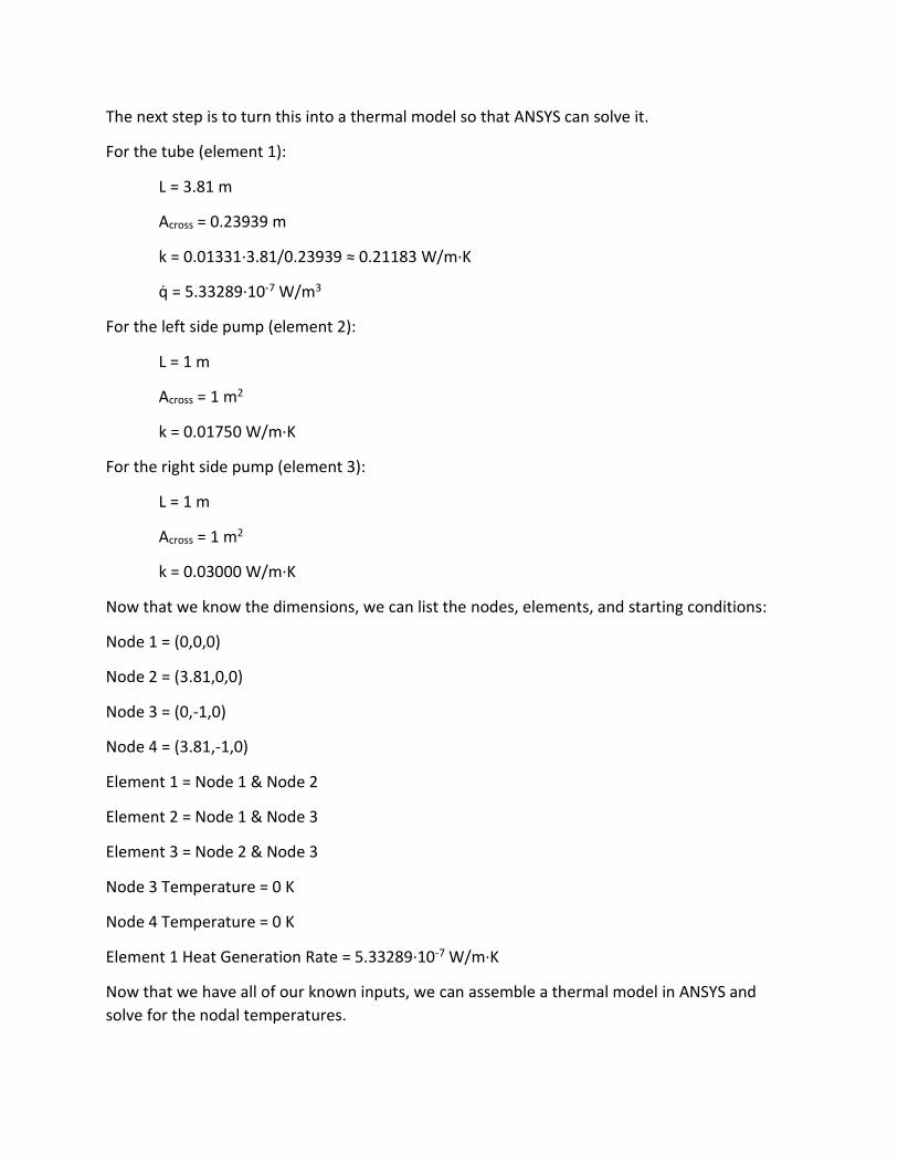
The next step is to turn this into a thermal model so that ANSYS can solve it.

For the tube (element 1):

L = 3.81 m

Across = 0.23939 m

k = 0.01331·3.81/0.23939 ≈ 0.21183 W/m·K

q̇ = 5.33289·10-7 W/m3

For the left side pump (element 2):

L = 1 m

Across = 1 m2

k = 0.01750 W/m·K

For the right side pump (element 3):

L = 1 m

Across = 1 m2

k = 0.03000 W/m·K

Now that we know the dimensions, we can list the nodes, elements, and starting conditions:

Node 1 = (0,0,0)

Node 2 = (3.81,0,0)

Node 3 = (0,-1,0)

Node 4 = (3.81,-1,0)

Element 1 = Node 1 & Node 2

Element 2 = Node 1 & Node 3

Element 3 = Node 2 & Node 3

Node 3 Temperature = 0 K

Node 4 Temperature = 0 K

Element 1 Heat Generation Rate = 5.33289·10-7 W/m·K

Now that we have all of our known inputs, we can assemble a thermal model in ANSYS and

solve for the nodal temperatures.

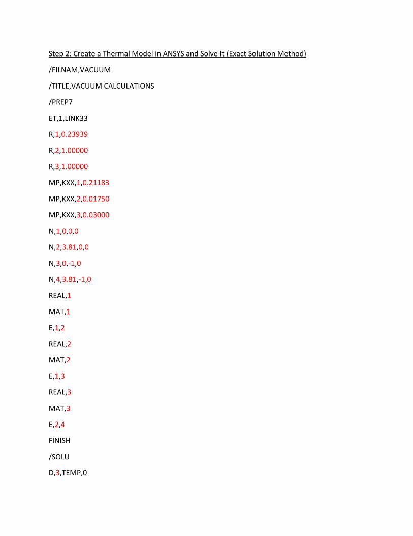
Step 2: Create a Thermal Model in ANSYS and Solve It (Exact Solution Method)

/FILNAM,VACUUM

/TITLE,VACUUM CALCULATIONS

/PREP7

ET,1,LINK33

R,1,0.23939

R,2,1.00000

R,3,1.00000

MP,KXX,1,0.21183

MP,KXX,2,0.01750

MP,KXX,3,0.03000

N,1,0,0,0

N,2,3.81,0,0

N,3,0,-1,0

N,4,3.81,-1,0

REAL,1

MAT,1

E,1,2

REAL,2

MAT,2

E,1,3

REAL,3

MAT,3

E,2,4

FINISH

/SOLU

D,3,TEMP,0

D,4,TEMP,0

BFE,1,HGEN,1,5.33289E-7

ANTYPE,STATIC

SAVE

SOLVE

FINISH

/POST1

PLNSOL,TEMP

PRNSOL,TEMP

PRESOL,HEAT

FINISH

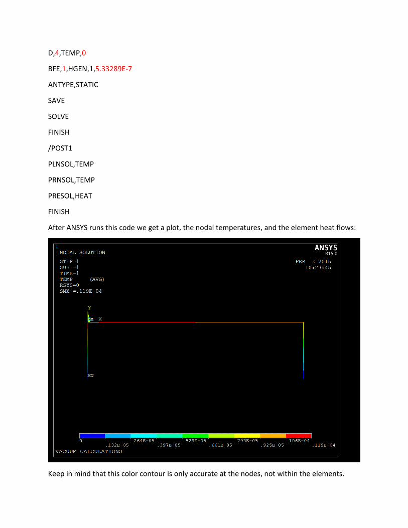
After ANSYS runs this code we get a plot, the nodal temperatures, and the element heat flows:

Keep in mind that this color contour is only accurate at the nodes, not within the elements.

PRINT TEMP NODAL SOLUTION PER NODE

***** POST1 NODAL DEGREE OF FREEDOM LISTING *****

LOAD STEP= 1 SUBSTEP= 1

TIME= 1.0000 LOAD CASE= 0

NODE TEMP

1 0.11899E-04

2 0.92722E-05

3 0.0000

4 0.0000

MAXIMUM ABSOLUTE VALUES

NODE 1

VALUE 0.11899E-04

PRINT HEAT ELEMENT SOLUTION PER ELEMENT

***** POST1 ELEMENT NODE TOTAL FORCE LISTING *****

LOAD STEP= 1 SUBSTEP= 1

TIME= 1.0000 LOAD CASE= 0

ELEM= 1 HEAT

1 0.20824E-06

2 0.27816E-06

ELEM= 2 HEAT

1 -0.20824E-06

3 0.20824E-06

ELEM= 3 HEAT

2 -0.27816E-06

4 0.27816E-06

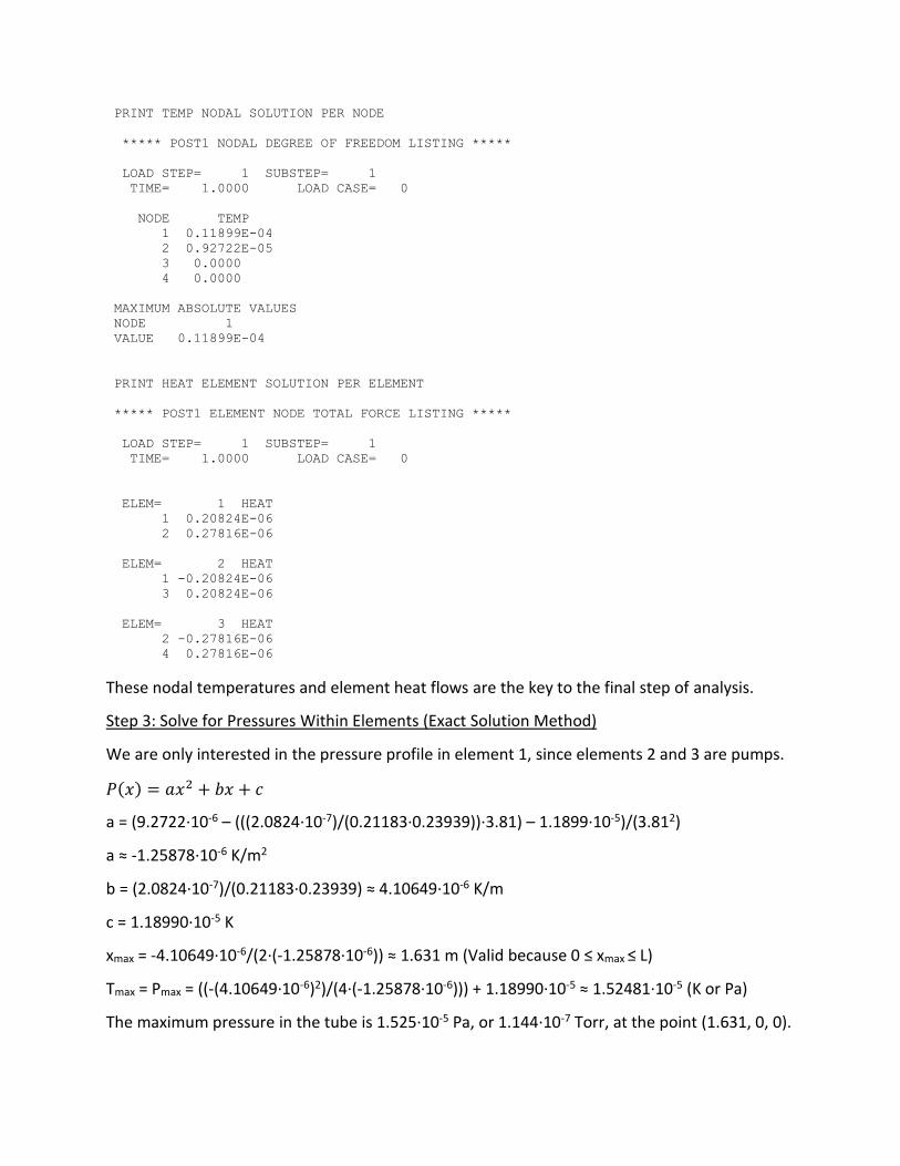
These nodal temperatures and element heat flows are the key to the final step of analysis.

Step 3: Solve for Pressures Within Elements (Exact Solution Method)

We are only interested in the pressure profile in element 1, since elements 2 and 3 are pumps.

𝑃(𝑥) = 𝑎𝑥2 + 𝑏𝑥 + 𝑐

a = (9.2722·10-6 – (((2.0824·10-7)/(0.21183·0.23939))·3.81) – 1.1899·10-5)/(3.812)

a ≈ -1.25878·10-6 K/m2

b = (2.0824·10-7)/(0.21183·0.23939) ≈ 4.10649·10-6 K/m

c = 1.18990·10-5 K

xmax = -4.10649·10-6/(2·(-1.25878·10-6)) ≈ 1.631 m (Valid because 0 ≤ xmax ≤ L)

Tmax = Pmax = ((-(4.10649·10-6)2)/(4·(-1.25878·10-6))) + 1.18990·10-5 ≈ 1.52481·10-5 (K or Pa)

The maximum pressure in the tube is 1.525·10-5 Pa, or 1.144·10-7 Torr, at the point (1.631, 0, 0).

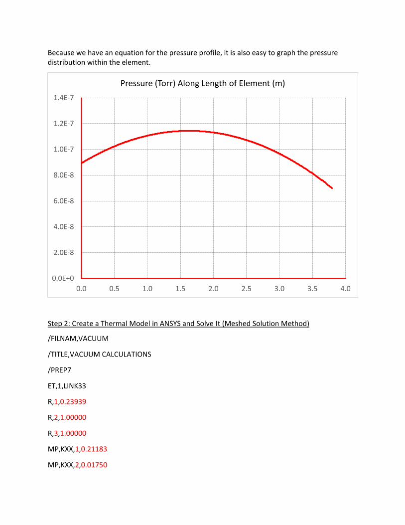
Because we have an equation for the pressure profile, it is also easy to graph the pressure distribution within the element.

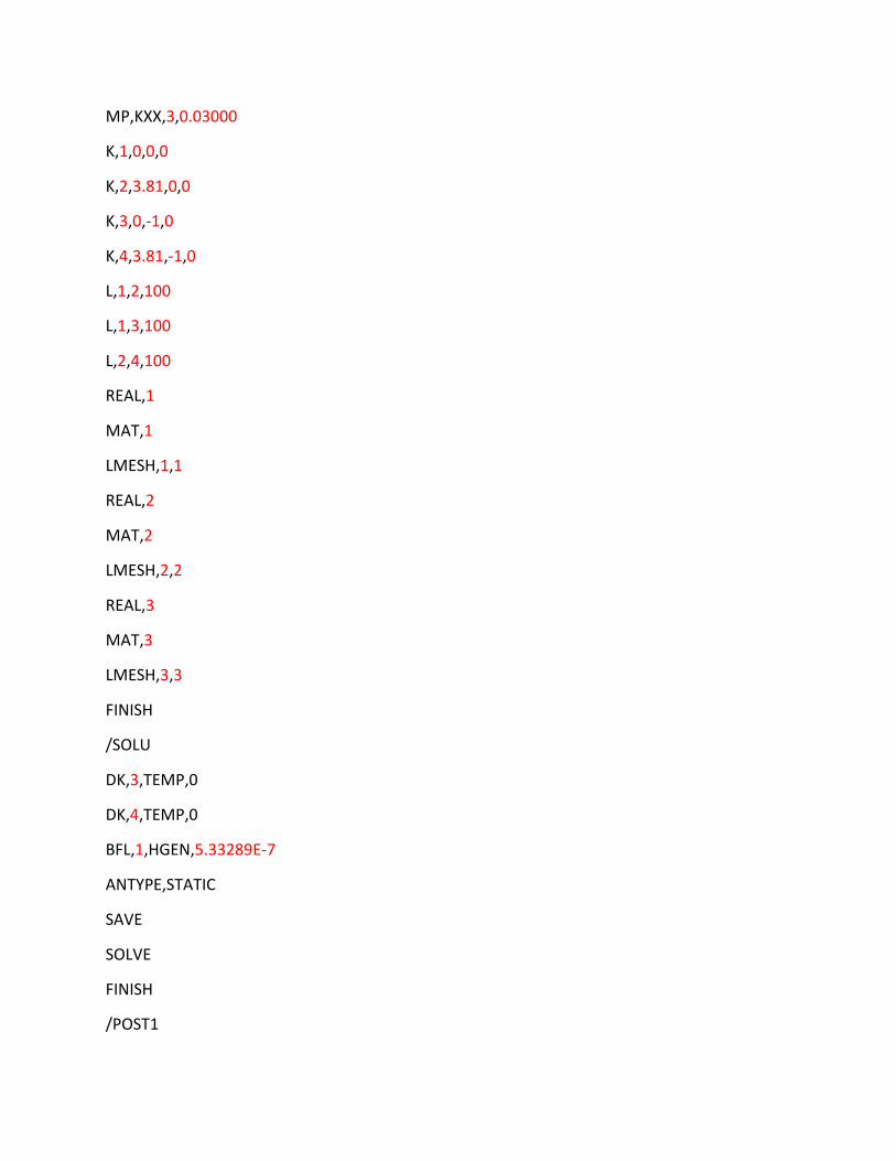
Step 2: Create a Thermal Model in ANSYS and Solve It (Meshed Solution Method)

/FILNAM,VACUUM

/TITLE,VACUUM CALCULATIONS

/PREP7

ET,1,LINK33

R,1,0.23939

R,2,1.00000

R,3,1.00000

MP,KXX,1,0.21183

MP,KXX,2,0.01750

0.0E+0

2.0E-8

4.0E-8

6.0E-8

8.0E-8

1.0E-7

1.2E-7

1.4E-7

0.0 0.5 1.0 1.5 2.0 2.5 3.0 3.5 4.0

Pressure (Torr) Along Length of Element (m)

MP,KXX,3,0.03000

K,1,0,0,0

K,2,3.81,0,0

K,3,0,-1,0

K,4,3.81,-1,0

L,1,2,100

L,1,3,100

L,2,4,100

REAL,1

MAT,1

LMESH,1,1

REAL,2

MAT,2

LMESH,2,2

REAL,3

MAT,3

LMESH,3,3

FINISH

/SOLU

DK,3,TEMP,0

DK,4,TEMP,0

BFL,1,HGEN,5.33289E-7

ANTYPE,STATIC

SAVE

SOLVE

FINISH

/POST1

PLNSOL,TEMP

PRNSOL,TEMP

PRESOL,HEAT

FINISH

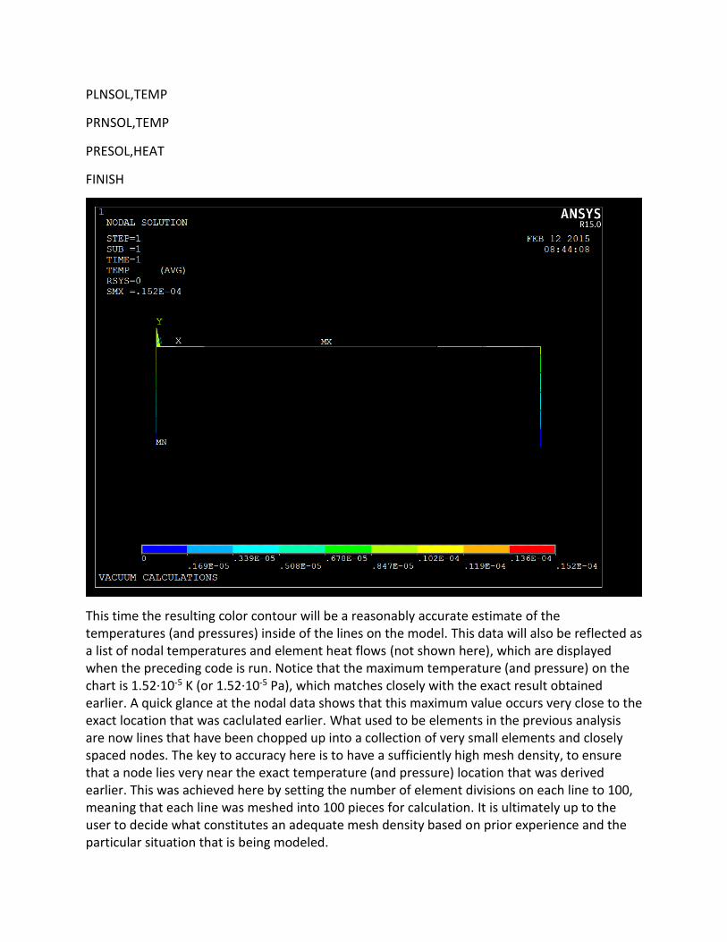
This time the resulting color contour will be a reasonably accurate estimate of the temperatures (and pressures) inside of the lines on the model. This data will also be reflected as a list of nodal temperatures and element heat flows (not shown here), which are displayed when the preceding code is run. Notice that the maximum temperature (and pressure) on the chart is 1.52·10-5 K (or 1.52·10-5 Pa), which matches closely with the exact result obtained earlier. A quick glance at the nodal data shows that this maximum value occurs very close to the exact location that was caclulated earlier. What used to be elements in the previous analysis are now lines that have been chopped up into a collection of very small elements and closely spaced nodes. The key to accuracy here is to have a sufficiently high mesh density, to ensure that a node lies very near the exact temperature (and pressure) location that was derived earlier. This was achieved here by setting the number of element divisions on each line to 100, meaning that each line was meshed into 100 pieces for calculation. It is ultimately up to the user to decide what constitutes an adequate mesh density based on prior experience and the particular situation that is being modeled.

References

Howell, J., B. Wehrle, and H. Jostlein. "Calculation of Pressure Distribution in Vacuum Systems Using a Commercial Finite Element Program." Conference Record of the 1991 IEEE Particle Accelerator Conference: Accelerator Science and Technology, May 6-9, 1991, San Francisco, California. Vol. 4. New York, NY: IEEE, 1991. 2295-2297. Print.

Lafferty, J. M. Foundations of Vacuum Science and Technology. New York: Wiley, 1998. Print.

Roth, A. Vacuum Technology. 2nd ed. Amsterdam: North-Holland Pub., 1982. Print.