Performing Bayesian Performing Bayesian Inference Inference

by Weighted Model by Weighted Model CountingCounting

Tian Sang, Paul Beame, and Henry Tian Sang, Paul Beame, and Henry KautzKautz

Department of Computer Science & EngineeringDepartment of Computer Science & Engineering

University of WashingtonUniversity of Washington

Seattle, WASeattle, WA

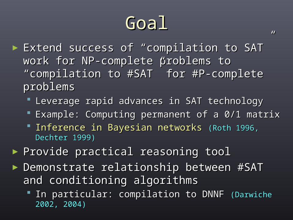
GoalGoal► Extend success of “compilation to SAT” work Extend success of “compilation to SAT” work

for NP-complete problems to “compilation to for NP-complete problems to “compilation to #SAT” for #P-complete problems#SAT” for #P-complete problems Leverage rapid advances in SAT technologyLeverage rapid advances in SAT technology Example: Computing permanent of a 0/1 matrixExample: Computing permanent of a 0/1 matrix Inference in Bayesian networks Inference in Bayesian networks (Roth 1996, Dechter (Roth 1996, Dechter

1999)1999)

► Provide practical reasoning toolProvide practical reasoning tool► Demonstrate relationship between #SAT Demonstrate relationship between #SAT

and conditioning algorithmsand conditioning algorithms In particular: compilation to DNNF In particular: compilation to DNNF (Darwiche 2002, (Darwiche 2002,

2004)2004)

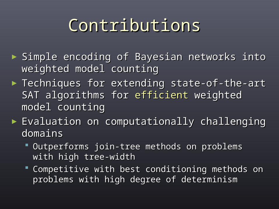
Contributions Contributions

► Simple encoding of Bayesian networks into Simple encoding of Bayesian networks into weighted model countingweighted model counting

► Techniques for extending state-of-the-art SAT Techniques for extending state-of-the-art SAT algorithms for algorithms for efficientefficient weighted model weighted model countingcounting

► Evaluation on computationally challenging Evaluation on computationally challenging domainsdomains Outperforms join-tree methods on problems with Outperforms join-tree methods on problems with

high tree-widthhigh tree-width Competitive with best conditioning methods on Competitive with best conditioning methods on

problems with high degree of determinismproblems with high degree of determinism

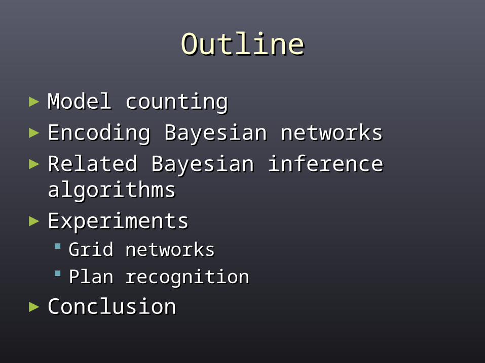
OutlineOutline

►Model countingModel counting►Encoding Bayesian networksEncoding Bayesian networks►Related Bayesian inference Related Bayesian inference

algorithmsalgorithms►ExperimentsExperiments

Grid networksGrid networks Plan recognitionPlan recognition

►ConclusionConclusion

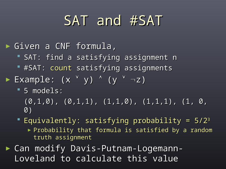
SAT and #SATSAT and #SAT

► Given a CNF formula, Given a CNF formula, SAT: find a satisfying assignment nSAT: find a satisfying assignment n #SAT: #SAT: countcount satisfying assignments satisfying assignments

► Example: (x Example: (x y) y) (y (y z)z) 5 models: 5 models:

(0,1,0), (0,1,1), (1,1,0), (1,1,1), (1, 0, 0)(0,1,0), (0,1,1), (1,1,0), (1,1,1), (1, 0, 0) Equivalently: satisfying probability = 5/2Equivalently: satisfying probability = 5/233

► Probability that formula is satisfied by a random truth Probability that formula is satisfied by a random truth assignmentassignment

► Can modify Davis-Putnam-Logemann-Can modify Davis-Putnam-Logemann-Loveland to calculate this valueLoveland to calculate this value

DPLL for SATDPLL for SATDPLL(F)DPLL(F)

if F is empty, return 1if F is empty, return 1if F contains an empty clause, return 0if F contains an empty clause, return 0else choose a variable x to branchelse choose a variable x to branch return (DPLL(F|return (DPLL(F|x=1x=1) V DPLL(F|) V DPLL(F|x=0x=0))))

#DPLL for #SAT#DPLL for #SAT#DPLL(F)#DPLL(F) // computes satisfying probability of F// computes satisfying probability of F

if F is empty, return 1if F is empty, return 1if F contains an empty clause, return 0if F contains an empty clause, return 0else choose a variable x to branchelse choose a variable x to branch return return 0.5*#DPLL(F|0.5*#DPLL(F|x=1 x=1 )) + 0.5*#DPLL(F|+ 0.5*#DPLL(F|

x=0x=0))

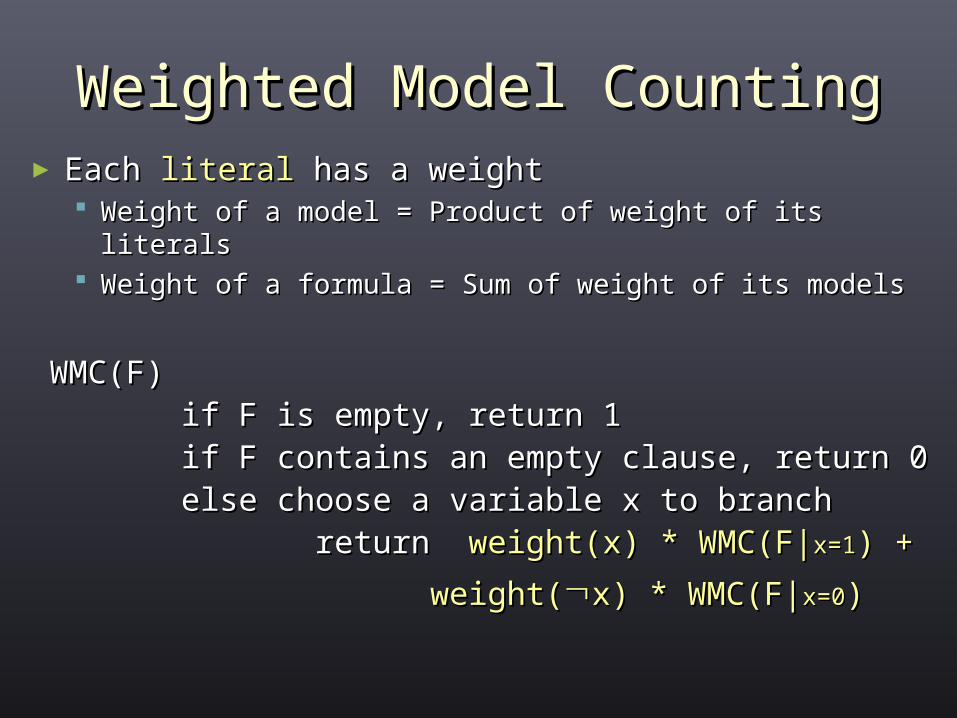
Weighted Model CountingWeighted Model Counting► Each Each literalliteral has a weight has a weight

Weight of a model = Product of weight of its Weight of a model = Product of weight of its literalsliterals

Weight of a formula = Sum of weight of its modelsWeight of a formula = Sum of weight of its models

WMC(F)WMC(F)if F is empty, return 1if F is empty, return 1if F if F contains an empty clausecontains an empty clause, return 0, return 0else choose a variable x to branchelse choose a variable x to branch return return weight(x) * WMC(F|weight(x) * WMC(F|x=1x=1) + ) +

weight(weight(x) * WMC(F|x) * WMC(F|x=0x=0))

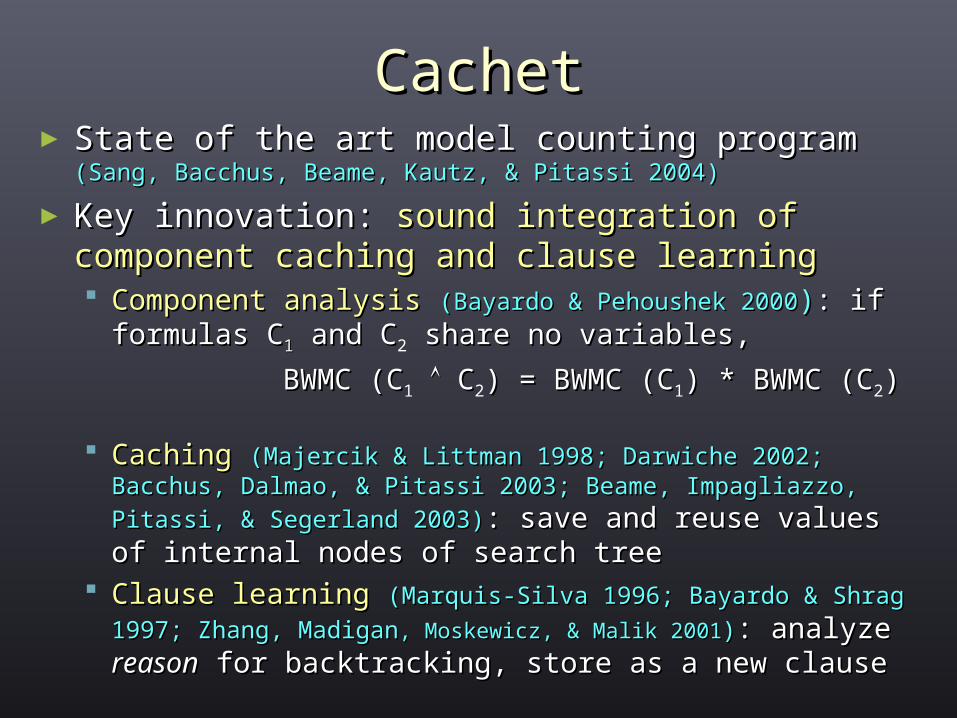
CachetCachet► State of the art model counting program State of the art model counting program

(Sang, Bacchus, Beame, Kautz, & Pitassi 2004)(Sang, Bacchus, Beame, Kautz, & Pitassi 2004)

► Key innovation: Key innovation: sound integration of sound integration of component caching and clause learningcomponent caching and clause learning Component analysisComponent analysis (Bayardo & Pehoushek 2000(Bayardo & Pehoushek 2000)): if : if

formulas Cformulas C11 and C and C2 share no variables, share no variables,

BWMC (CBWMC (C1 C C2) = BWMC (C) = BWMC (C1) * BWMC (C) * BWMC (C2))

Caching Caching (Majercik & Littman 1998; Darwiche 2002; (Majercik & Littman 1998; Darwiche 2002; Bacchus, Dalmao, & Pitassi 2003; Beame, Impagliazzo, Bacchus, Dalmao, & Pitassi 2003; Beame, Impagliazzo, Pitassi, & Segerland 2003)Pitassi, & Segerland 2003): save and reuse values of : save and reuse values of internal nodes of search treeinternal nodes of search tree

Clause learningClause learning (Marquis-Silva 1996; Bayardo & Shrag (Marquis-Silva 1996; Bayardo & Shrag

1997; Zhang, Madigan1997; Zhang, Madigan, Moskewicz, & Malik 2001, Moskewicz, & Malik 2001)): analyze : analyze reasonreason for backtracking, store as a new clause for backtracking, store as a new clause

CachetCachet► State of the art model counting program State of the art model counting program

(Sang, Bacchus, Beame, Kautz, & Pitassi 2004)(Sang, Bacchus, Beame, Kautz, & Pitassi 2004)

► Key innovation: Key innovation: sound integration of sound integration of component caching and clause learningcomponent caching and clause learning

Naïve combination of all three techniques is Naïve combination of all three techniques is unsoundunsound

Can resolve by careful cache management Can resolve by careful cache management (Sang, (Sang, Bacchus, Beame, Kautz, & Pitassi 2004)Bacchus, Beame, Kautz, & Pitassi 2004)

New branching strategy (VSADS) optimized for New branching strategy (VSADS) optimized for counting counting (Sang, Beame, & Kautz SAT-2005)(Sang, Beame, & Kautz SAT-2005)

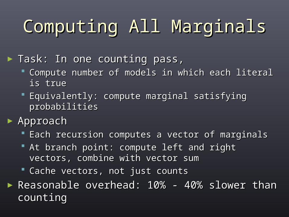
Computing All MarginalsComputing All Marginals

► Task: In one counting pass,Task: In one counting pass, Compute number of models in which each literal is Compute number of models in which each literal is

truetrue Equivalently: compute marginal satisfying Equivalently: compute marginal satisfying

probabilitiesprobabilities

► ApproachApproach Each recursion computes a vector of marginalsEach recursion computes a vector of marginals At branch point: compute left and right vectors, At branch point: compute left and right vectors,

combine with vector sumcombine with vector sum Cache vectors, not just countsCache vectors, not just counts

► Reasonable overhead: 10% - 40% slower than Reasonable overhead: 10% - 40% slower than countingcounting

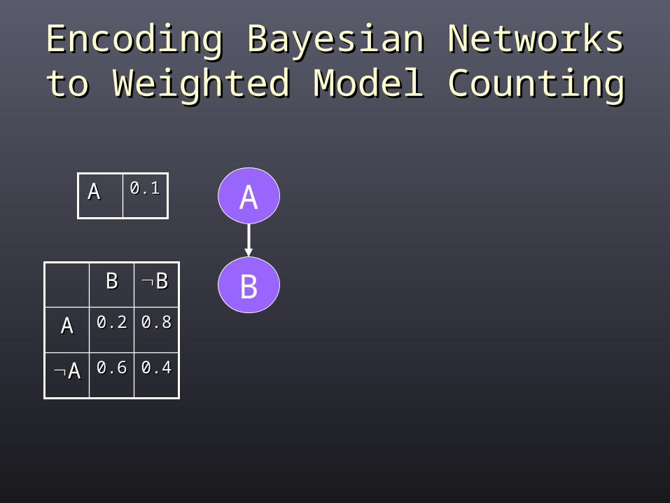
Encoding Bayesian Networks to Encoding Bayesian Networks to Weighted Model CountingWeighted Model Counting

A

B0.80.80.20.2AA

0.40.40.60.6AA

BBBB

0.10.1A A

Encoding Bayesian Networks to Encoding Bayesian Networks to Weighted Model CountingWeighted Model Counting

A

B0.80.80.20.2AA

0.40.40.60.6AA

BBBB

0.10.1A A

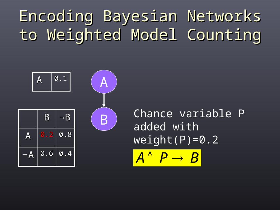
BPA

Chance variable P added with weight(P)=0.2

Encoding Bayesian Networks to Encoding Bayesian Networks to Weighted Model CountingWeighted Model Counting

A

B0.80.80.20.2AA

0.40.40.60.6AA

BBBB

0.10.1A A

BPA

and weight(P)=0.8P)=0.8

Encoding Bayesian Networks to Encoding Bayesian Networks to Weighted Model CountingWeighted Model Counting

A

B0.80.80.20.2AA

0.40.40.60.6AA

BBBB

0.10.1A A

BQA

Chance variable Q added with weight(Q)=0.6

Encoding Bayesian Networks to Encoding Bayesian Networks to Weighted Model CountingWeighted Model Counting

A

B0.80.80.20.2AA

0.40.40.60.6AA

BBBB

0.10.1A A

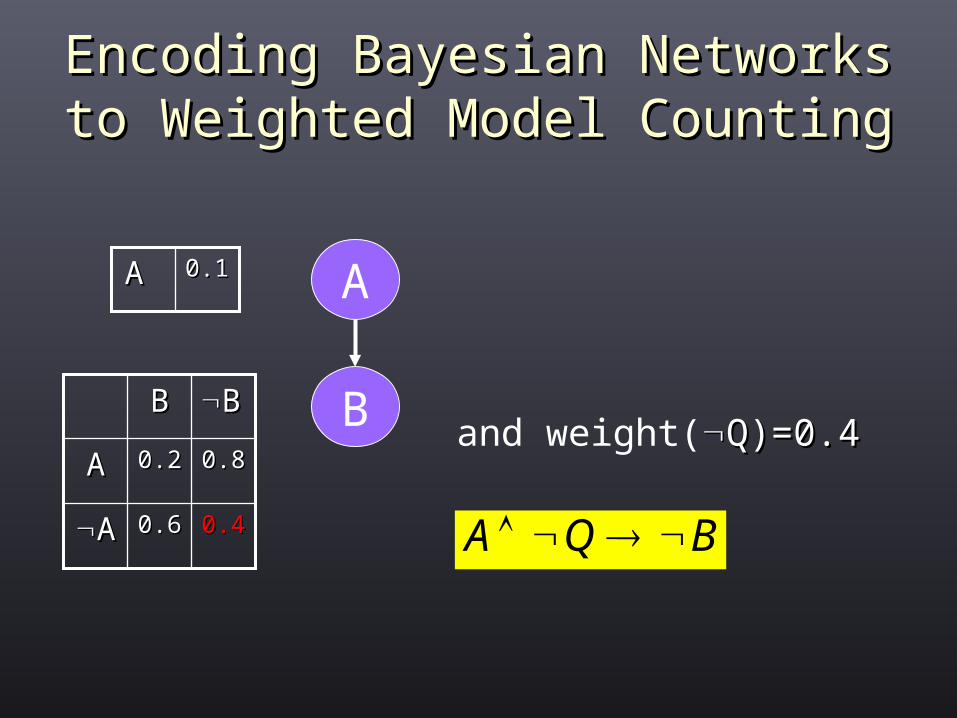
BQA

and weight(Q)=0.4Q)=0.4

Encoding Bayesian Networks to Encoding Bayesian Networks to Weighted Model CountingWeighted Model Counting

A

B0.80.80.20.2AA

0.40.40.60.6AA

BBBB

0.10.1A A

BPA

BPA

BQA

BQA

w(A)=0.1w(A)=0.1 w(w(A)=0.9A)=0.9

w(P)=0.2w(P)=0.2 w(w(P)=0.8P)=0.8

w(Q)=0.6w(Q)=0.6 w(w(Q)=0.4Q)=0.4

w(B)=1.0w(B)=1.0 w(w(B)=1.0B)=1.0

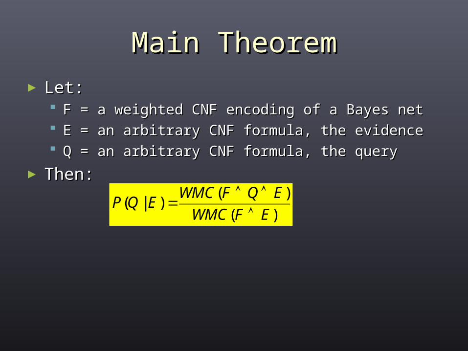
Main TheoremMain Theorem► Let:Let:

F = a weighted CNF encoding of a Bayes netF = a weighted CNF encoding of a Bayes net E = an arbitrary CNF formula, the evidenceE = an arbitrary CNF formula, the evidence Q = an arbitrary CNF formula, the queryQ = an arbitrary CNF formula, the query

► Then:Then:( )

( | )( )

WMC F Q EP Q E

WMC F E

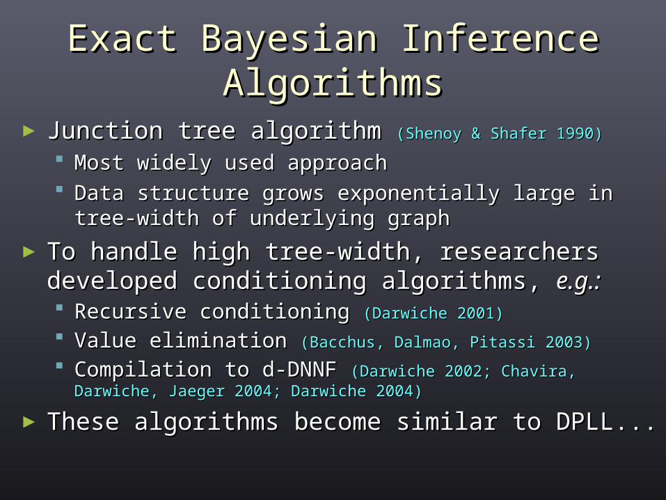
Exact Bayesian Inference Exact Bayesian Inference AlgorithmsAlgorithms

► Junction tree algorithm Junction tree algorithm (Shenoy & Shafer 1990)(Shenoy & Shafer 1990)

Most widely used approachMost widely used approach Data structure grows exponentially large in tree-Data structure grows exponentially large in tree-

width of underlying graphwidth of underlying graph

► To handle high tree-width, researchers To handle high tree-width, researchers developed conditioning algorithms, developed conditioning algorithms, e.g.:e.g.: Recursive conditioning Recursive conditioning (Darwiche 2001)(Darwiche 2001)

Value elimination Value elimination (Bacchus, Dalmao, Pitassi 2003)(Bacchus, Dalmao, Pitassi 2003)

Compilation to d-DNNF Compilation to d-DNNF (Darwiche 2002; Chavira, Darwiche, (Darwiche 2002; Chavira, Darwiche, Jaeger 2004; Darwiche 2004)Jaeger 2004; Darwiche 2004)

► These algorithms become similar to DPLL...These algorithms become similar to DPLL...

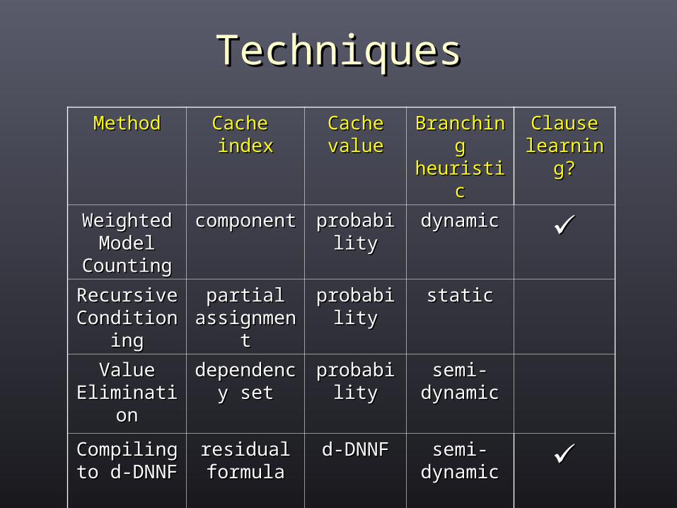
TechniquesTechniques

MethodMethod Cache Cache indexindex

Cache Cache valuevalue

BranchinBranchingg

heuristicheuristic

Clause Clause learning?learning?

Weighted Weighted Model Model

CountingCounting

componencomponentt

probabiliprobabilityty

dynamicdynamic

Recursive Recursive ConditioniConditioni

ngng

partialpartialassignmenassignmen

tt

probabiliprobabilityty

staticstatic

Value Value EliminatioEliminatio

nn

dependencdependency sety set

probabiliprobabilityty

semi-semi-dynamicdynamic

Compiling Compiling to d-DNNFto d-DNNF

residualresidualformulaformula

d-DNNFd-DNNF semi-semi-dynamicdynamic

ExperimentsExperiments

►Our benchmarks: Grid, Plan RecognitionOur benchmarks: Grid, Plan Recognition Junction tree - NeticaJunction tree - Netica Recursive conditioning – SamIamRecursive conditioning – SamIam Value elimination – ValelimValue elimination – Valelim Weighted model counting – CachetWeighted model counting – Cachet

► ISCAS-85 and SATLIB benchmarksISCAS-85 and SATLIB benchmarks Compilation to d-DNNF – timings from Compilation to d-DNNF – timings from

(Darwiche 2004)(Darwiche 2004) Weighted model counting - CachetWeighted model counting - Cachet

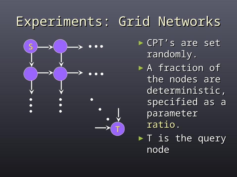
Experiments: Grid NetworksExperiments: Grid Networks

S

T

►CPT’s are set CPT’s are set randomly.randomly.

►A fraction of the A fraction of the nodes are nodes are deterministic, deterministic, specified as a specified as a parameter parameter ratioratio. .

►T is the query T is the query nodenode

Results of ratio=0.5Results of ratio=0.5

SizeSize JunctionJunctionTreeTree

RecursiveRecursiveConditioninConditionin

gg

ValueValueEliminationElimination

Weighted Weighted ModelModel

CountingCounting

10*1010*10 0.020.02 0.880.88 2.02.0 7.37.3

12*1212*12 0.550.55 1.61.6 15.415.4 3838

14*1414*14 2121 7.97.9 8787 419419

16*1616*16 XX 104104 >20,861>20,861 890890

18*1818*18 XX 2,1262,126 XX 13,11113,111

10 problems of each size, X=memory out or time out

Results of ratio=0.75Results of ratio=0.75SizeSize JunctionJunction

TreeTreeRecursiveRecursive

ConditioninConditioningg

ValueValueEliminationElimination

Weighted Weighted ModelModel

CountingCounting

12*1212*12 0.470.47 1.51.5 1.41.4 1.01.0

14*1414*14 21202120 1515 8.38.3 4.74.7

16*1616*16 >227>227 9393 7171 3939

18*1818*18 XX 1,7511,751 >1,053>1,053 8181

20*2020*20 XX >24,02>24,0266

>94,99>94,9977

248248

22*2222*22 XX XX XX 1,3001,300

24*2424*24 XX XX XX 4,9984,998

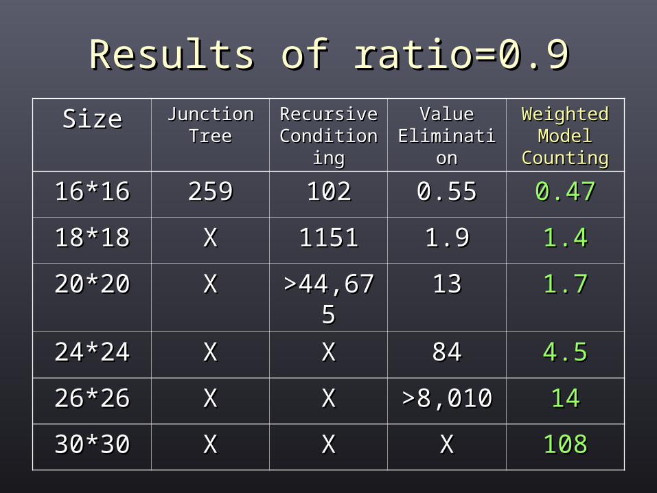
Results of ratio=0.9Results of ratio=0.9

SizeSize JunctionJunctionTreeTree

RecursiveRecursiveConditioninConditionin

gg

ValueValueEliminationElimination

Weighted Weighted ModelModel

CountingCounting

16*1616*16 259259 102102 0.550.55 0.470.47

18*1818*18 XX 11511151 1.91.9 1.41.4

20*2020*20 XX >44,67>44,6755

1313 1.71.7

24*2424*24 XX XX 8484 4.54.5

26*2626*26 XX XX >8,010>8,010 1414

30*3030*30 XX XX XX 108108

Plan RecognitionPlan Recognition►Task: Task:

Given a planning domain described by Given a planning domain described by STRIPS operators, initial and goal states, and STRIPS operators, initial and goal states, and time horizontime horizon

Infer the marginal probabilities of each Infer the marginal probabilities of each actionaction

►Abstraction of strategic plan recognition: Abstraction of strategic plan recognition: We know enemy’s capabilities and We know enemy’s capabilities and goals, what will it do?goals, what will it do?

►Modified Blackbox planning system Modified Blackbox planning system (Kautz & Selman 1999)(Kautz & Selman 1999) to create instances to create instances

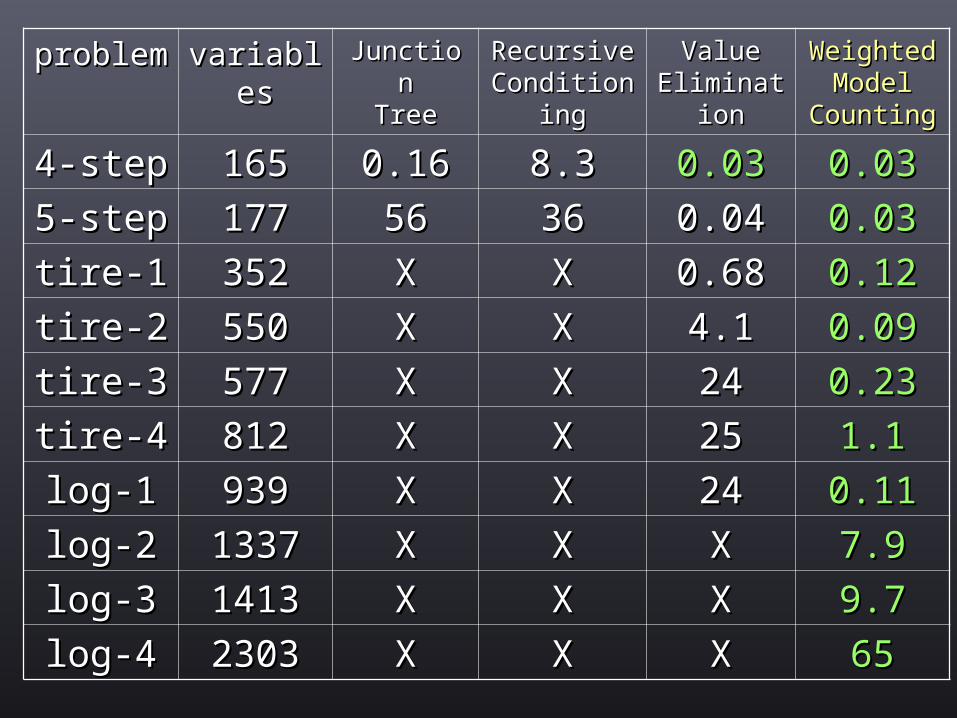
problemproblem variablevariabless

JunctionJunctionTreeTree

RecursiveRecursiveConditioniConditioni

ngng

ValueValueEliminatiEliminati

onon

Weighted Weighted ModelModel

CountingCounting

4-step4-step 165165 0.160.16 8.38.3 0.030.03 0.030.03

5-step5-step 177177 5656 3636 0.040.04 0.030.03

tire-1tire-1 352352 XX XX 0.680.68 0.120.12

tire-2tire-2 550550 XX XX 4.14.1 0.090.09

tire-3tire-3 577577 XX XX 2424 0.230.23

tire-4tire-4 812812 XX XX 2525 1.11.1

log-1log-1 939939 XX XX 2424 0.110.11

log-2log-2 13371337 XX XX XX 7.97.9

log-3log-3 14131413 XX XX XX 9.79.7

log-4log-4 23032303 XX XX XX 6565

ISCAS/SATLIB BenchmarksISCAS/SATLIB BenchmarksBenchmarks reportedBenchmarks reported

in in (Darwiche 2004)(Darwiche 2004)Compiling Compiling to d-DNNFto d-DNNF

WeighteWeightedd

ModelModelCountingCounting

uf200 (100 instances)uf200 (100 instances) 1313 77

flat200 (100 instances)flat200 (100 instances) 5050 88

c432c432 0.10.1 0.10.1

c499c499 66 8585

c880c880 8080 17,50617,506

c1355c1355 1515 7,0577,057

c1908c1908 187187 1,8551,855

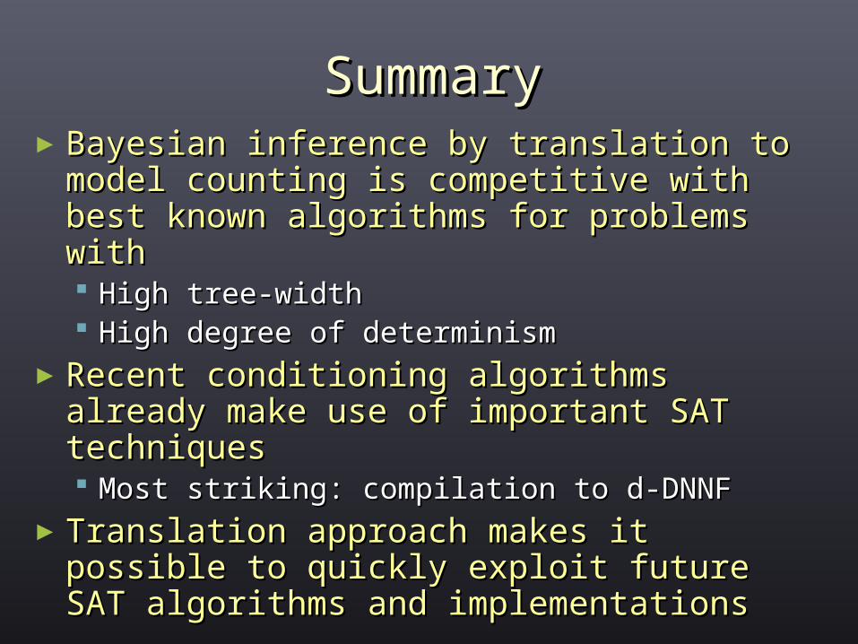
SummarySummary►Bayesian inference by translation to Bayesian inference by translation to

model counting is competitive with model counting is competitive with best known algorithms for problems best known algorithms for problems withwith High tree-widthHigh tree-width High degree of determinismHigh degree of determinism

►Recent conditioning algorithms already Recent conditioning algorithms already make use of important SAT techniquesmake use of important SAT techniques Most striking: compilation to d-DNNFMost striking: compilation to d-DNNF

►Translation approach makes it possible Translation approach makes it possible to quickly exploit future SAT algorithms to quickly exploit future SAT algorithms and implementationsand implementations