Embed Size (px)
Citation preview
PERFORMANCE TRACKING & CHARACTERIZATION OF COMMERCIAL
SOLAR PANELS
A THESIS SUBMITTED TO
THE GRADUATE SCHOOL OF NATURAL AND APPLIED SCIENCES
OF
MIDDLE EAST TECHNICAL UNIVERSITY
BY
CELAL GÜVENÇ OGULGÖNEN
IN PARTIAL FULFILLMENT OF THE REQUIREMENTS
FOR
THE DEGREE OF MASTER OF SCIENCE
IN
CHEMICAL ENGINEERING
FEBRUARY 2014


iv
Approval of thesis:
PERFORMANCE TRACKING & CHARACTERIZATION OF COMMERCIAL SOLAR PANELS
submitted by C. GÜVENÇ OGULGÖNEN in partial fulfillment of the requirements for the degree of Master of Science in Chemical Engineering Department, Middle East Technical University by, Prof. Dr. Canan Özgen ___________________________ Dean, Graduate School of Natural and Applied Sciences Prof. Dr. Halil Kalıpçılar ___________________________ Head of Department, Chemical Engineering Asst.Prof. Dr. Serkan Kıncal ___________________________ Supervisor, Chemical Engineering Dept., METU Examining Committee Members: Prof. Dr. İnci Eroğlu ___________________________ Chemical Engineering Dept., METU Asst.Prof. Dr. Serkan Kıncal ___________________________ Chemical Engineering Dept., METU Prof. Dr. Raşit Turan ___________________________ Physics Dept., METU Assoc. Prof. Dr. Görkem Külah ___________________________ Chemical Engineering Dept., METU Eyüp Tongel ___________________________ ASELSAN
Date: 12.02.2014

iv
I hereby declare that all information in this document has been obtained and
presented in accordance with academic rules and ethical conduct. I also declare
that, as required by these rules and conduct, I have fully cited and referenced
all material and results that are not original to this work.
Name, Last name: C. Güvenç OGULGÖNEN
Signature:

v
ABSTRACT
PERFORMANCE TRACKING & CHARACTERIZATION OF COMMERCIAL
SOLAR PANELS
Ogulgönen, C. Güvenç
M. Sc. Department of Chemical Engineering
Supervisor: Asst. Prof. Serkan Kıncal
February 2014, 147 pages
This study aims to characterize the performance of different types of commercial
solar panels in terms of the meteorological parameters such as irradiance,
temperature, pressure, relative humidity with the technologies of mono and
polycrystalline along with thin film, by evaluating the performance data collected
with a Daystar MT-5 I-V curve tracer. The approach to this characterization is a
comprehensive data collection scheme where solar panel performance is monitored
side-by-side with an exhaustive list of atmospheric conditions gathered by the HOBO
U30 Weather Station for two and a half years in the atmospheric conditions of
Ankara. In addition to that, a light soaking station for accelerated module testing is
designed, constructed and tested with the sample solar cells. Statistical analysis are
made to calculate and evaluate the global performance metrics such as performance
ratio and light soaking station successfully tracked and showed the change of
performance for the sample cells.
Keywords: Photovoltaic cells, solar energy,degradation mechanism,performance
modeling

vi
ÖZ
TİCARİ GÜNEŞ PANELLERİNİN PERFORMANS TAKİBİ VE
KARAKTERİZASYONU
Ogulgönen, C. Güvenç
Yüksek Lisans, Kimya Mühendisliği Bölümü
Tez Yöneticisi:Yrd. Doç. Dr. Serkan Kıncal
Şubat 2014, 147 sayfa
Bu çalışma, monokristal, polikristal, ince film gibi farklı teknolojilerde üretilmiş
endüstriyel güneş panellerinin sıcaklık, güneş ışıması, basınç, bağıl nem gibi
meteorolojik değişkenlere bağlı olarak performans karakterizasyonunun Daystar MT-
5 I-V eğrisi takip ekipmanının topladığı veriler ile değerlendirilmesini
amaçlamaktadır. Karakterizasyon yaklaşımı, çok sayıda veri toplanması ile aynı dış
şartlara maruz bırakılan güneş panellerinin meteorolojik değişkenlere göre HOBO
Meteoroloji Ekipmanı ile iki buçuk yıl boyunca Ankara şehri atmosfer şartlarında
toplanan verilerin değerlendirilmesini içermektedir. Bunun yanında, bir güneş paneli
yaşlandırma ünitesi tasarlanmış, inşa edilmiş ve örnek güneş gözeleri ile operasyonu
test edilmiştir. Evrensel düzeyde Kabul edilen performans oranı gibi parametreler
istatistiksel analizlerle hesaplanmış, karşılaştırılmış ve yaşlandırma ünitesi başarılı
bir şekilde örnek gözelerin performansını takip edip değişimleri gözlemlemeyi
mümkün kılmıştır.
Anahtar Kelimeler: Fotovoltaik hücreler, güneş enerjisi, bozunma mekanizmaları,
performans modellemesi

vii
To my family

viii
ACKNOWLEDGEMENTS
Firstly, I would like to thank to my supervisor Asst. Prof. Dr. Serkan Kıncal for his
great help on the thinking process and the hard work he put for this study. Without
his great vision, guidance, understanding and belief in me, I would not have the
motivation to go through this process.
I am grateful to Prof. Raşit Turan and The Center for Solar Energy Research and
Applications (GÜNAM) for providing me the biggest support to conduct this study
in a healthy and creative environment with all the tools needed.
Thank you Prof. Üner, for the ideas you seeded to our brains, for giving me the
inspiration to start my graduate work and the motivation for writing my thesis. I
promise I am going to fill the notebook that you gave to me with useful information.
I would also like to thank to my friends; Memo, Ata, Neco, İbo, Can, 2 Burcus, Must
and all Block C residents for their endless support and for the laughs that make our
days less boring most of the time. Without the things we shared, I would not be as
happy as I am now, for sure.
I should also mention the staffs of our department Ertuğrul Özdemir, Süleyman Nazif
Kuşhan, Adil Demir, İsa Çağlar, Mustafa Cansuyu for letting me learn from their
technical knowledge and for the physical work they put together for this study. They
are very good at what they do and they are also very kind and nice people to anyone
willing to learn and share.
I also thank Assoc. Prof. Çerağ Dilek for her kindness and big effort to make my
thesis writing process easier.
Apart from all of the valuable people above, my deepest gratitude, coming from my
soul, are to my parents. Their unlimited love, support and confidence in me
throughout my life made me who I am now.

ix
TABLE OF CONTENTS
ABSTRACT ................................................................................................. v
ÖZ ............................................................................................................... vi
ACKNOWLEDGEMENTS ......................................................................viii
TABLE OF CONTENTS............................................................................ ix
LIST OF FIGURES ..................................................................................xiii
LIST OF TABLES ................................................................................... xvii
1. LITERATURE SURVEY AND BACKGROUND ....................................... 1
1.1. Different Photovoltaic Technologies ........................................................... 1
1.1.1. Crystalline silicon ...................................................................................... 2
1.1.1.1. Single crystal silicon ............................................................................. 4
1.1.1.1.1. Czochralski Growth (CZ): .................................................................. 5
1.1.1.1.2. Float Zone Method (FZ):.................................................................... 5
1.1.1.2. Multi crystal silicon .............................................................................. 6
1.1.2. Thin film .................................................................................................... 9
1.1.2.1. Amorphous silicon ................................................................................ 9
1.1.2.2. Cadmium telluride (CdTe) ................................................................. 11
1.1.2.3. Copper Indium Gallium Diselenide (CIGS) ....................................... 11
1.1.2.4. Group III-V ......................................................................................... 12
1.2. Panel Degradation Mechanisms ................................................................ 13
1.2.1. Overview for Common Degradation Modes ........................................... 13
1.2.2. Physical Degradation Modes ................................................................... 19
1.2.2.1. Corrosion ............................................................................................ 19
1.2.2.2. Discoloration ...................................................................................... 20
1.2.2.3. Glass soiling: ...................................................................................... 21
1.2.2.4. Delamination ...................................................................................... 22

x
1.2.2.4.1. Front- side delamination: .................................................................. 23
1.2.2.4.2. Front grid and AR coating: ............................................................... 23
1.2.2.4.3. Bubbles: ............................................................................................ 24
1.2.2.5. Breakage and cracking cells ............................................................... 25
1.2.2.6. Potential Induced Degradation (PID) ................................................. 26
1.2.2.7. Hot spots ............................................................................................. 27
1.2.2.8. Mismatched Cells ............................................................................... 27
1.2.2.9. Temperature Induced Degradation ..................................................... 28
1.2.3. Light Induced Degradation ...................................................................... 31
1.3. Performance Characterization Studies – Outdoor Testing Stations ........... 37
1.3.1. PV Module I – V Characteristics............................................................. 37
1.3.2. Effect of the type of PV technology ........................................................ 39
1.3.3. Ambient temperature ............................................................................... 40
1.3.4. Solar Irradiation ....................................................................................... 40
1.3.5. Tilt Angle................................................................................................. 41
1.3.6. Others ...................................................................................................... 41
1.3.7. Evaluation of the PV Performance .......................................................... 41
1.3.7.1. Final yield (YF) .................................................................................. 42
1.3.7.2. Reference Yield (YR) ......................................................................... 42
1.3.7.3. Performance Ratio .............................................................................. 43
1.3.7.4. PVUSA Rating.................................................................................... 43
1.3.7.5. Capacity Factor (CF) .......................................................................... 44
1.3.7.6. System Efficiency ............................................................................... 44
1.3.8. Outdoor Studies ....................................................................................... 44
1.4. Accelerated Testing in Light Soaking Station ........................................... 49
1.4.1. Xenon Arc Lamps: .................................................................................. 50
1.4.2. Fluorescent UV Lamps and Devices: ...................................................... 52
1.4.3. Metal Halide Lamps ................................................................................ 54
2. EXPERIMENTAL SETUP .......................................................................... 57
xi
2.1. HOBO U30 Station .................................................................................... 59
2.1.1. U30 Station Components ........................................................................ 59
2.1.1.1. HOBO U30 Ethernet Data Logger ..................................................... 59
2.1.1.2. Solar Radiation Sensor (Silicon Pyranometer) S – LIB – M003 ........ 61
2.1.1.3. Rain Gauge Smart Sensor S – RGA – M002 ..................................... 61
2.1.1.4. Temperature and Relative Humidity (RH) Smart Sensor .................. 62
2.1.1.5. Wind Direction Smart Sensor S – WDA – M003 .............................. 63
2.1.1.6. Wind Speed Smart Sensor S – WMA – M003 ................................... 65
2.1.2. HOBOlink ............................................................................................... 65
2.2. Daystar Multi – Tracer............................................................................... 73
2.3. StellarNet Blue – Wave Spectrometer ....................................................... 78
2.4. FTP Server ................................................................................................. 80
2.5. Solar Module List and Justifications ......................................................... 82
2.5.1. Solar Modules List .................................................................................. 83
3. LIGHT SOAKING STATION DESIGN ..................................................... 85
3.1. Overview of the Design ............................................................................. 85
3.2. Choice of the Light Source ........................................................................ 85
3.3. Choice of Instrumentation ......................................................................... 88
3.4. Lamp Configuration and Station Housing Design .................................... 89
3.4.1. Single Light Source Characterization...................................................... 91
3.4.2. Multiple Light Source Modeling ............................................................. 93
3.5. Finalized Design and Equipment ............................................................... 96
4. RESULTS AND ANALYSIS ...................................................................... 99
4.1. PV Performance Monitoring Station Analysis .......................................... 99
4.1.1. Data Integrity Issues ................................................................................ 99

xii
4.1.1.1. Missing Data and Corrupt Sensor Problems ....................................... 99
4.1.1.2. Design Upgrade for Spectrophotometer (Shutter Arrangement) ...... 100
4.1.2. Trend Analysis on Historical Climatic Data ......................................... 100
4.1.3. Correction for Module Tilt .................................................................... 112
4.1.3.1. Determination of the Tilt Correction ................................................ 112
4.1.3.2. Yearly Trends of Solar Position ....................................................... 114
4.1.4. Analysis of Solar Panel Performances .................................................. 117
4.2. LID Station Measurements ...................................................................... 126
4.2.1. Light Intensity Measurements ............................................................... 126
4.2.2. Test Run of the Light Soaking Station .................................................. 130
4.3. Future Improvements ............................................................................... 134
5. SUMMARY AND CONCLUSIONS ........................................................ 135 REFERENCES ........................................................................................ 137

xiii
LIST OF FIGURES
Figure 1-1 Basic Flowchart for Crystalline PV Cell Production [8] ............................ 3
Figure 1-2 Mono crystalline solar cell (left) and simplified cross-section of a mono
crystalline solar cell (right)[6] ...................................................................................... 4
Figure 1-3 Single crystal pattern .................................................................................. 5
Figure 1-4 Structure of Polycrystalline Cell ................................................................ 6
Figure 1-5 Polycrystalline silicon solar cell ................................................................. 7
Figure 1-6 Crystalline Silicon Cell Production Steps Overview[6] ............................. 8
Figure 1-7 Cross-section of a-Si solar cell ................................................................. 10
Figure 1-8 Cross-section of CdTe cell ....................................................................... 11
Figure 1-9 Cross-section of CIGS cell ....................................................................... 12
Figure 1-10 Circuit representation of a solar cell ...................................................... 14
Figure 1-11 A highly browned EVA encapsulation on a crystalline cell [29] ........... 16
Figure 1-12 An example of layers of a photovoltaic module [34] ............................. 17
Figure 1-13 Encapsulation of a PV module [35] ....................................................... 17
Figure 1-14 Failure modes of PV modules caused by packaging material and
detection methods....................................................................................................... 18
Figure 1-15 Visible corrosion at the edge of the cell ................................................. 20
Figure 1-16 Discoloured solar cell [47] ..................................................................... 21
Figure 1-17 Haziness that could be seen at the edge of the cell ................................ 22
Figure 1-18 Delaminated photovoltaic module [47] .................................................. 23
Figure 1-19 A PV module with bubbles on the back side [39] .................................. 24
Figure 1-20 AR coating oxidation through the center of the cell .............................. 25
Figure 1-21 Severely broken glass on a polycrystalline PV module [59].................. 26
Figure 1-22 Hot spot formation ................................................................................. 27
Figure 1-23 Busbars help prevent the cracked cell producing lower current (a)crack
removing the part of the cell from the circuit (b) ....................................................... 28
Figure 1-24 Ambient Temperature Efficiency Relation ............................................ 32
Figure 1-25 Electric Field for the Layers of CdTe Cells ........................................... 34

xiv
Figure 1-26 Efficiency vs Time at Different Temperatures for a CdTe Cell ............. 34
Figure 1-27 Effect of Cu Addition ............................................................................. 35
Figure 1-28 Suggested Mechanism of Cu Diffusion .................................................. 35
Figure 1-29 CIGS Cross - Section .............................................................................. 36
Figure 1-30 Single diode model of a PV cell ............................................................. 37
Figure 1-31 Spectral distribution of a commercial Xenon lamp ................................ 51
Figure 1-32 Spectral distributions of a commercial Xenon lamp with different filters
.................................................................................................................................... 52
Figure 1-33 Spectral distribution of UV – A&B lamps and sunlight ........................ 53
Figure 1-34 UV – A vs Sunlight behind the glass...................................................... 54
Figure 1-35 Spectral distribution of a commercial metal halide lamp with the sunlight
spectrum ..................................................................................................................... 55
Figure 2-1 Data Acquisition Flowchart ...................................................................... 58
Figure 2-2 HOBO Weather Station ............................................................................ 60
Figure 2-3 HOBO U30 Data Logger .......................................................................... 60
Figure 2-4 Silicon Pyranometer S – LIB – M003 ...................................................... 62
Figure 2-5 Rain Gauge Smart Sensor ......................................................................... 63
Figure 2-6 Temperature and RH Smart Sensor .......................................................... 63
Figure 2-7 Wind Direction Smart Sensor ................................................................... 64
Figure 2-8 Wind Speed Smart Sensor ........................................................................ 65
Figure 2-9 Wind Speed & Direction Sensor Combined ............................................. 66
Figure 2-10 Devices Tab Screenshot ......................................................................... 67
Figure 2-11 An Overview of Graphs .......................................................................... 67
Figure 2-12 Latest Conditions Pane ........................................................................... 68
Figure 2-13 Latest Data Pane ..................................................................................... 68
Figure 2-14 A Sample .dtf File View from HOBOware ............................................ 69
Figure 2-15 Latest Connections Tab .......................................................................... 69
Figure 2-16 Device Informatioın Pane ....................................................................... 70
Figure 2-17 Device Configuration Menu ................................................................... 70
Figure 2-18 Launch Configuration Menu .................................................................. 71
Figure 2-19 Readout Configuration Menu ................................................................. 72

xv
Figure 2-20 Go to Alarms Menu ................................................................................ 72
Figure 2-21 Daystar MT 5.......................................................................................... 73
Figure 2-22 Load and Control Units of Daystar MT5 ............................................... 74
Figure 2-23 Web Server for MT5 .............................................................................. 75
Figure 2-24 Settings Menu and Average Interval ...................................................... 76
Figure 2-25 Peak Power Setting ................................................................................. 76
Figure 2-26 FTP Server Screen for MT – 5 ............................................................... 77
Figure 2-27 Index of .mtd and .xml Files................................................................... 77
Figure 2-28 StellarNet Blue -Wave Spectrometer ..................................................... 78
Figure 2-29 Screenshot from SpectraWiz. Episodic Data Capture with Two Different
Spectometers .............................................................................................................. 78
Figure 2-30 UVN Spectra of Sunlight ....................................................................... 79
Figure 2-31 Entrance Screen for FTP Server ............................................................. 81
Figure 2-32 Datascreen in the FTP Server ................................................................. 81
Figure 2-33 HOBO Folder and Files .......................................................................... 82
Figure 2-34 All panels in the station .......................................................................... 82
Figure 2-35 Daystar MT – 5 load (below) and control unit (top) .............................. 83
Figure 3-1 The patented light soaking design [114] .................................................. 86
Figure 3-2 Side and Top view of LID Station ........................................................... 86
Figure 3-3 Spectral Distribution for Xe Flash Lamp [115] ....................................... 87
Figure 3-4 Spectral Distribution of a Metal Halide Lamp [116] ............................... 88
Figure 3-5 Picture of the Chassis with the cards installed ......................................... 89
Figure 3-6 Picture of the single light source and the starter ...................................... 91
Figure 3-7 Single light source intensity distributions - intensity measurements are in
terms of w/m2 and grid data are in terms of cm. ........................................................ 92
Figure 3-8 Various orientations of the 9 lamps considered ....................................... 93
Figure 3-9 Distribution at 45 cm lamp separation and 50 cm between the lamps and
the panels .................................................................................................................... 95
Figure 3-10 Average intensity as a function of separation - inverse square behavior 96
Figure 3-11 The Final Construction of the Light Soaking Stat .................................. 98
Figure 4-1 Shutter Design ........................................................................................ 101

xvi
Figure 4-2 Reference Temperature Data throughout 2010 – 2013 .......................... 102
Figure 4-3 Reference Solar Irradiation Data throughout 2010 – 2013 .................... 103
Figure 4-4 Temperature Data Comparison ............................................................... 104
Figure 4-5 Pressure Data Comparison ..................................................................... 104
Figure 4-6 Relative Humidity Data Comparison ..................................................... 105
Figure 4-7 Wind Speed Data Comparison ............................................................... 106
Figure 4-8 Wind Direction Data Comparison .......................................................... 107
Figure 4-9 Solar Irradiance Data Comparison ......................................................... 108
Figure 4-10 Solar Irradiance Data Comparison for Below Region .......................... 109
Figure 4-11 Solar Irradiance Data Comparison for Above Region ......................... 110
Figure 4-12 Corrected HOBO Irradiance vs. Reference .......................................... 111
Figure 4-13 Solar Zenith Angle ............................................................................... 116
Figure 4-14 Tilt Correction Factors by Time of day, colored by month .................. 117
Figure 4-15 Maximum Power vs. Short Circuit Current for Installed Panels ......... 120
Figure 4-16 Maximum Power vs. Open Circuit Voltage for Installed Panels ......... 121
Figure 4-17 Maximum Power vs Fill Factor for Installed Panels ............................ 121
Figure 4-18 Maximum Power vs Series Resistance for Installed Panels ................. 122
Figure 4-19 Maximum Power vs Shunt Resistance for Installed Panels ................. 123
Figure 4-20 Performance Ratio Comparison ........................................................... 123
Figure 4-21 Performance Ratio vs Temperature for Installed Panels ...................... 126
Figure 4-22 Performance Ratio vs Relative Humidity for Installed Panels ............. 127
Figure 4-23 Performance Ratio vs Pressure for Installed Panels ............................. 127
Figure 4-24 Light Intensity as a Function of Time at 47 cm Table to Lamp Separation
.................................................................................................................................. 128
Figure 4-25 Typical Contour Plots ........................................................................... 129
Figure 4-26 Temperature vs Time Plot for Different Points in the LID Station ...... 131
Figure 4-27 Time Period when the Cooling Fans are Turned off ............................ 131
Figure 4-28 I- V Curve under Different Illuminations for 1 Cell Module ............... 132
Figure 4-29 I - V Curve under Different Illuminations for 4 Cell Module .............. 133
Figure 4-30 Voc Change for 4 Cell Module ............................................................ 133
Figure 4-31 Voc Temperature Relationship for 4 Cell Module ............................... 134

xvii
LIST OF TABLES
Table 1-1: Main categorization for PV technologies [3] ............................................. 1
Table 1-2 Crystal Grain Sizes of Common PV Technologies ..................................... 3
Table 1-3 Summary of key characteristics of commercial PV modules .................... 13
Table 1-4 Physical Degradation Modes Breakdown [65] .......................................... 29
Table 1-5 Thin-film failure modes and mechanisms [66] .......................................... 30
Table 1-6 STC, SOC and NOC Definitions ............................................................... 39
Table 1-7 Summary of Outdoor Station Findings ...................................................... 48
Table 0-1 List of Installed Solar Modules.................................................................. 84
Table 3-1 Summary of the simulation results ............................................................ 97
Table 4-1 Summary for Correction Values of Meteorological Parameters ............. 111
Table 4-2 Summary of Data Points .......................................................................... 119
Table 4-3 Grouping Radiation Levels ...................................................................... 119
Table 4-4 Statistical Comparison of Panel Performance Ratios .............................. 125
Table 4-5 Summary Statistics for Light Intensity Distribution ................................ 130


1
CHAPTER 1
1. LITERATURE SURVEY AND BACKGROUND
1.1. Different Photovoltaic Technologies
Photovoltaics are used in several different markets namely, satellites,
telecommunications, cathodic protections which requires DC voltages for the
corrosion prevention purposes for metals, water pumping and treatment in remote
regions, solar home systems, energy need in remote houses, consumer products like
battery chargers with certain power needs as well as grid connected power supply
systems.[1] Photovoltaic technologies could be categorized like Table 1-1 below.
Crystalline silicon and thin film technologies are the most widely used modules
while there are other applications like organic/polymer, hybrid and dye-sensitized
solar cells. Therefore, photovoltaic technologies can be categorized under three main
groups: [2]
Table 1-1: Main categorization for PV technologies [3]
2
1.1.1. Crystalline silicon
Crystalline silicon (c-Si) modules occupy 85-90% of the global PV market [4].
Crystalline silicon is the most commonly used technology for commercial
applications. It has advantages of having a very well known standardized processing
and having an abundant source of feedstock silicon. The main disadvantages for
crystalline silicon technology are the need for high purity, therefore expensive silicon
and having a competition in terms of feedstock with the electronics industry.
Basically, crystalline solar cells have many different types varying from non-
crystalline to multi crystalline technologies. The main categorization could be
summarized as below;
Current commercial single crystal solar modules have conversions around 14 to 20%
and their efficiency is expected to rise up to 23% until 2020. [5]
There are three main industries that are related to the crystalline silicon solar cell and
module production:
- Metallurgical and chemical silicon production plants
- Ingot and wafer fabrication facilities for crystalline solar cell (mono and poly)
- Solar cell and module production facilities
The cost division for the crystalline solar cell modules could be roughly divided to
50% for silicon substrate, 20% for processing the cell and 30% for the processing of
the module. Therefore, the price of the silicon remains as the most important cost
parameter for the PV industry. [6]
The main differences between these technologies are the crystal grain size and
different techniques that are used for growing the crystals.

3
Table 1-2 Crystal Grain Sizes of Common PV Technologies
Crystal Type Symbol Crystal Grain
Size
Common Growth
Technique
Single crystal sc-Si >10 cm Czochralski (Cz)
Float-Zone (FZ)
Multicrystalline mc-Si 10 cm Cast, Spheral, Sheet,
Ribbon
Polycrystalline pc-Si 1 μm – 1 mm Evaporation, CVD,
sputtering
Manufacture of c-Si modules involve steps including growing ingots of silicon,
slicing the ingots into wafers for the formation of solar cells, establishing the
connections between cells and making the necessary encapsulation for the cells to
form a complete module with reasonable voltage and current values.
Figure 1-1Figure 1.1 shows the main steps mentioned above for the production of a
crystalline solar module. [7]
Figure 1-1 Basic Flowchart for Crystalline PV Cell Production [8]

4
Three types of silicon are mainly used in this procedure: single crystalline silicon (sc-
Si), multi crystalline silicon (mc-Si) and ribbon sheet crystal (c-Si). [9]
1.1.1.1. Single crystal silicon
Single (mono) crystalline cell modules constitute the 80% of the PV market. Single
crystalline silicon is produced by crystal growth techniques. Solar cells with the
reasonable performance parameters are generally produced by using silicon. Silicon
has an indirect band gap of 1.1eV having indirect band gap causes silicon to have
low light absorption, but this problem could be overcome by using a silicon with
several hundred microns thickness and purifying it for reducing the defects in the
crystal structure for decreasing rate of recombination therefore allowing minority
carriers penetrate to the depletion region without high losses. [10]
Single crystalline silicon cells have some advantages. By using this technology,
efficiencies around 20% could be achieved. [11] Single crystal cells are mainly
produced for electronics industry. On the other hand, they require a high purity feed
stock (around 99.9% pure silicon). Along with the production method and feedstock
qualities, single crystal modules require higher cost for production with a slower
process line. In addition to that, feedstock is wasted in a greater rate because of the
circular shape of the cells and that also leads to lower packing density in panels. In
single crystal form, all atoms are arranged in the same pattern. There are two
commercial production techniques for single crystal silicon cells:
Figure 1-2 Mono crystalline solar cell (left) and simplified cross-section of a mono
crystalline solar cell (right)[6]

5
Figure 1-3 Single crystal pattern
1.1.1.1.1. Czochralski Growth (CZ):
Most of the single crystal silicon cells are manufactured by CZ Growth Technique. It
provides lower quality silicon than FZ with oxygen and carbon on the cell. However,
it is cheaper compared to the FZ Growth and produces cylinders and circular wafers.
In CZ Growth, pure silicon is melted in a quartz crucible under vacuum or inert gas
environment and a seed crystal is dipped into the melt. After this, the seed is slowly
taken out by slowly rotating in order to make the crystallization over the seed by the
molten silicon. By adjusting the temperature, rotation and pulling rate, ingot size
could be altered. One big crystal is formed as ingot and it has high purity and very
few defects. The crystal does not include any boundaries since it is purely one crystal
with only one orientation shown above. However, the crystal includes oxygen
contaminated from the quartz crucible.
1.1.1.1.2. Float Zone Method (FZ):
The production is made on the cylindrical poly silicon rod. This special rod contains
a seed in its lower end. A heating rod circling the rod starts to melt the silicon as it
starts melting at the bottom moving towards the top. A single solid ingot is formed in
the down region. Impurities stays in the molten part, therefore this method creates
very high purity and low number of defects.

6
After the crystal growth process, the ingots are cut into thin wafers having width of
300 μm. the cutting procedure is made by two main techniques:
Wire sawing
Diamond blade sawing
1.1.1.2. Multi crystal silicon
Multicrystalline silicon solar cells are manufactured using two different methods.
The first one is the ribbon silicon. In ribbon silicon technique, two filaments of
graphite are put in a crucible with molten silicon in it. Then, the molten silicon is
grown horizontally through capillary action between the filaments. This yields into a
sheet of multicrystalline wafer. The thickness of the multicrystalline wafer could be
adjusted by changing the width of the filament and the pulling speed. In addition to
that, this method is cheaper than growing single crystal growth techniques and less
silicon is wasted thanks to the change in the sawing methods (no circular shape is
needed). On the other hand, produced multicrystalline cells have lower efficiencies
compared to the single crystal cells because of the higher rate of defects and irregular
surface structure characteristics.
Figure 1-4 Structure of Polycrystalline Cell

7
Poly & Multi Silicon is the second method for multicrystalline growth. Crystal
growth is done in a large rectangular crucible by melting the silicon material. The
molten material is slowly cooled with the control of temperature and direction of the
cooling. Impurities in the molten material tend to place themselves on the edges
since the edges cool slower. After the cooling is done, the edges are cut and etched
off. These big blocks are then sliced into smaller blocks and then to the wafers.
Figure 1-5 Polycrystalline silicon solar cell
Multicrystalline silicon solar cells have crystal grains with different sizes. They are
cheaper to manufacture and processed faster than single crystal silicon cells.
However, they are less efficient than mono crystalline cells due to the grain
boundaries which cause electrical losses. The efficiency of the multicrystalline solar
cells is expected to reach up to 21% in the long term and crystalline modules are
expected to remain as the dominant technology until at least 2020. [12] The use of
hydrogen is very important during the processing of the multicrystalline cells
because hydrogen passivates the grain boundaries that cause electrical losses in the
device. This procedure is mostly done by the technique called PECVD (plasma
enhanced chemical vapor deposition) for the deposition of silicon nitride, which uses
hydrogen, instead of silicon dioxide. Multicrystaline silicon cells generally have
efficiencies 2-3% less than commercial silicon cells, however the cost of
manufacturing multicrystalline cells are 20% less than single crystalline cells. [13]

8
There are several techniques to remove avoid impurities in the multicrystalline solar
cell structure. One of them is the use of phosphorus getterings to bring the mobile
impurities to the surface. [14] In addition to that, immobile point defects could be
deactivated by the use of hydrogen passivation because atomic hydrogen could
diffuse into the silicon material even at low temperatures. [15] In PECVD, silicon
nitride antireflection coating is done using silane (SiH4) or ammonia (NH3) as the gas
source. These gases work as the hydrogen source for the diffusion of hydrogen into
the wafer. [16] Efficiencies of commercial multicrystalline silicon solar cells are
between 14-19%. [17]
Figure 1-6 Crystalline Silicon Cell Production Steps Overview[6]
The main difference between single and multi crystalline solar modules comes from
the crystal growth step. Silicon that is purified by using several procedures are
melted around 1400°C and a small crystal is cooled to be used as the seed for the
crystal growth. When the seed is pulled out, it starts to solidify at the interface with
the melt. If the pulling procedure is slow enough, the newly formed silicon atoms
could arrange themselves according to the crystal structure of the seed. This form is a

9
single-crystal silicon ingot. On the other hand, silicon ingots could be produced by
controlling the cooling rate of molten silicon while pouring it into a container. Ingots
produced using this method could still be used in the making of a solar cell, but could
not have the same quality with the previous mentioned crystal growth method.
Basically, what obtained after the process are many little crystals or grains that are
packed randomly instead of one large single crystal. Therefore, this is called multi
crystalline silicon which also shows difference in the specialties like crystallization
rate, ingot size and area. These ingots are then cut into wafers to form by using
various different methods. [18]
1.1.2. Thin film
Thin film solar cells are uses 1-10 microns of semiconductor instead of 200-300
microns as in crystalline types. Thin films are produced by the deposition of the
semiconductor onto a cheaper glass substrate. One of the main advantages over
crystalline solar cells is cost reduction in production of the cell thanks to use of cheap
glass and less semiconductor material. However, the technology is more difficult in
terms of producing good quality films that resulting in lower efficiencies compared
to the crystalline solar cells.
There are three main categories of solar cells under thin film technology:
1.1.2.1. Amorphous silicon
Amorphous silicon cells are made by evaporating silicon onto a glass. Therefore, the
orientation of the atoms becomes more random than the crystalline cells. Silicon has
more unbounded hydrogen atoms and these unbounded electrons easily attract the
impurities that result a decrease in the electrical performance of the cell. In order to
deactivate the formed dangling bond, hydrogen is added to the material. Silane (SiH4)
as the silicon source for the cell provides deposited hydrogen amount of ~%10.
Hydrogenated silicon behaves totally differently than the pure silicon since its
bandgap increases from 1.1 to 1.7 with improved electronic properties. However, this
amount of hydrogen causes cell to lose some of its performance right after the
sunlight exposure. [16]

10
For a-Si technology, cell efficiencies are around 13% while the module efficiency is
around 6-8%. [15]
Figure 1-7 Cross-section of a-Si solar cell
a-Si technology have some advantages like ability to absorb both low and high
intensity light. In addition to that, a-Si cells cost less than crystalline cells because of
the lower use of semiconductor material and using cheap glass as the surface for the
deposition. Lastly, high temperatures do not affect the a-Si cell performance
drastically. On the other hand, a-Si modules have lower efficiency compared to
crystal technology and material degradation occurs after the long period of use. One
other disadvantage of a-Si solar cells is the hazardous gases that are required for
production. These gases create problem after the lifetime of the cell is over, in the
termination and recycle procedure.

11
1.1.2.2. Cadmium telluride (CdTe)
p-type part of the cell is made by Cadmium and Telluride and n-type part is made by
Cadmium Sulfide. CdTe technology offers high efficiencies for thin film
technologies (over 16%). However, manufacturing requires high processing
temperatures and the module itself becomes unstable and easily degraded. As
mentioned above, toxicity is another problem for this technology. Cadmium is a
poisonous element and the disposal of the module is not cost effective. In addition to
that, CdTe cells are vulnerable to water penetration which causes degradation in
cell’s electrical performance.
Figure 1-8 Cross-section of CdTe cell
1.1.2.3. Copper Indium Gallium Diselenide (CIGS)
CIGS modules have extremely good light absorption rates (99% of the light is
absorbed in the first micron of the cell). That is because the elements used in the
technology are the optimal ones for PV applications in terms of their absorption
coefficients. Especially, the addition of Ga increases the light absorption band gap in
the solar spectrum. Performance of CIGS modules does not degrade over time and it
provides the highest efficiency values among the thin film technologies (19%).

12
Figure 1-9 Cross-section of CIGS cell
CIGS modules have the advantage of high efficiency, but Gallium and Indium are
the scarce and expensive elements. Another drawback is that the production
procedure requires high vacuum applications.
1.1.2.4. Group III-V
Group III-V cells are produced from the compounds of III and V group elements on
the periodic table. This technology is mostly used in the electronics industry and
space applications. They have very high efficiencies, but the production cost is very
high too. They can also create multi-junction cells in order to increase the efficiency
further. Gallium Arsenide (GaAs) and Indium Phosphide (InP) are the single junction
III-V cells. Best efficiency is around 27.6% in this single junction technology. These
cells have very high efficiencies and low weights and in addition to these, they are
durable to the damage that could be done by the cosmic radiation. However, they are
very expensive to produce and require materials that are not very abundant. Group
III-V cells are also used in creating multi-junction solar modules. Multi-junction
cells are basically the p-n junctions put on top of each other. Each junction has
different band gap energies, so different regions of the solar spectrum are absorbed in
each junction. Like GaAs and InP modules, multi-junction cells are very expensive
to produce and offer high efficiencies up to 35.2%. They are used widely in extra
terrestrial applications.

13
Table 1-3 Summary of key characteristics of commercial PV modules
Technology Material
thickness (μm)
Area
(m2)
Efficiency
(%)
Surface area
(m2)
Mono – c – Si 200 1.4 – 1.7
(typical) 14 – 20 ~7
Multi – c – Si 160
1.4 – 1.7
(typical)
2.5 (up to)
11 – 15 ~8
a – Si 1 ~1.5 4 – 8 ~15
a – Si / μc – Si 2 ~1.4 7 – 9 ~12
CdTe ~1 – 3 ~0.6 – 1 10 – 11 ~10
CIGS ~2 ~0.6 – 1 7 – 12 ~10
1.2. Panel Degradation Mechanisms
1.2.1. Overview for Common Degradation Modes
Serving life of a photovoltaic module mostly depend on the stability and durability to
corrosion of the construction parts of the cell itself since there are no moving parts on
a photovoltaic solar cell by default. The guaranteed lifetime of a solar module could
be around 20-25 years depending on the technology; however there are different
failure modes and degradation mechanisms that could decrease the lifetime of the
module. In most cases, these conditions that could decrease the performance and
lifetime of the cells result from temperature and water ingress into the module.
There are degradation and failure modes of PV modules that could cause a gradual
decrease in performance or a permanent overall loss in the performance of the

14
module for a long time. Gradual decrease in the performance of the module could be
caused by;
Increase in Rs due to decreased adherence of contacts or corrosion. The cause
is usually water vapor.
Decrease in Rsh due to metal migration through the p-n junction
Damaging of the antireflection coating.
Figure 1-10 Circuit representation of a solar cell
Iph: photogenerated current
Rsh: shunt resistance
Rs: series resistance
RL: load resistance
Ish: shunt current
The source of the series resistance could be resistances in the termination points of
junction box, resistances in connection between the cells, busbars or in emitter
regions. Series resistance decreases the voltage of the PV cell causing a decrease in
the general performance of the module. During the manufacturing and the design
process of the module, series resistance is decreased to a minimum level. However,
thermal cycling conditions in the outdoor environment causes series resistances to a
slow increase. [19]

15
Shunt resistance creates highly conductive regions in the solar cell, especially on the
edges.
Shunt resistance results in shunt current whose value is very different from the
intended load. This affects the cell performance badly especially at low intensity of
light. The main reason behind the shunt resistance is the defects in the crystal
structure of the cell or the impurities near the junctions. Shunt resistance problem in
thin film solar cells occurs after long time of exposure to light. [20]. If the number of
shunts increases in the cell, this leads to the increased effective shunt currents and
decreased shunt resistances. [21]
A photovoltaic module could under perform because of several reasons. It could be
due to shading of the module, or just a part of the cell by an object depending on the
position of the sun during the day. The front surface of the module, which actually
absorbs the sunlight, could be blocked by soiling and this may cause up to 10% of
performance loss on the average. In a multi module system, failure of one module
could happen or the interconnection between the modules could fail, however these
cause reversible power reductions.
When one module is considered, there could be short circuits at cell interconnections.
This is a common failure mode for thin film cells as the top and back contact is very
close to each other and this increases the chance of short circuits through pin holes or
from the damaged parts of the cell.
Another commonly observed failure mode is the open circuited cells due to the
cracking in the module. This may be due to several reasons such as;
Thermal stress
Damaged parts during the manufacture and assembly of the module.
These are called latent cracks because they can not be detected during the quality
control tests and failure occurs after some time. A cell could still operate after
cracking thanks to the interconnect cell busbars which are the parts of the cell to
protect the rigidity. Thermal stress and wind loading could cause interconnect open
circuit failures. There could be open circuits in the junction box and bus wiring parts
16
of the module. In module scale, the open circuits could be due to manufacturing
defects. After the module is exposed to outdoor conditions, the insulation material
could degrade. This results in the delamination, cracks or corrosions. There could be
serious cracks of the front glass of the module due to handling issues, harsh outdoor
conditions like strong wind, heavy rain or snow and mostly hail. Delamination
problem could occur mostly due to the weakening of the bond strength. The cause to
the weakening could be the physical conditions like weather or photothermal aging
and stress by moisture which causes irregular expansions on the structure of the parts
of the cells and module. Hot spots could occur after the mismatch, cracks or shading
happens meaning the high temperature gradients around the certain regions of the
cell or between the cells. Bypass diodes are used to avoid the overheating problem.
UV light could cause encapsulant material to lose its concentration and rigidity as the
aging happens. Encapsulant failure could happen although UV absorbers and some
encapsulant stabilizers could increase the lifetime of the encapsulant material.
Leaching and diffusion could cause the encapsulation material to degrade and EVA
browning because of the acetic acid formation could cause the performance of arrays
of modules gradually, especially in concentrating systems. [22] [23] EVA browning
issue is a problem that has been observed since 1980s. However, what is responsible
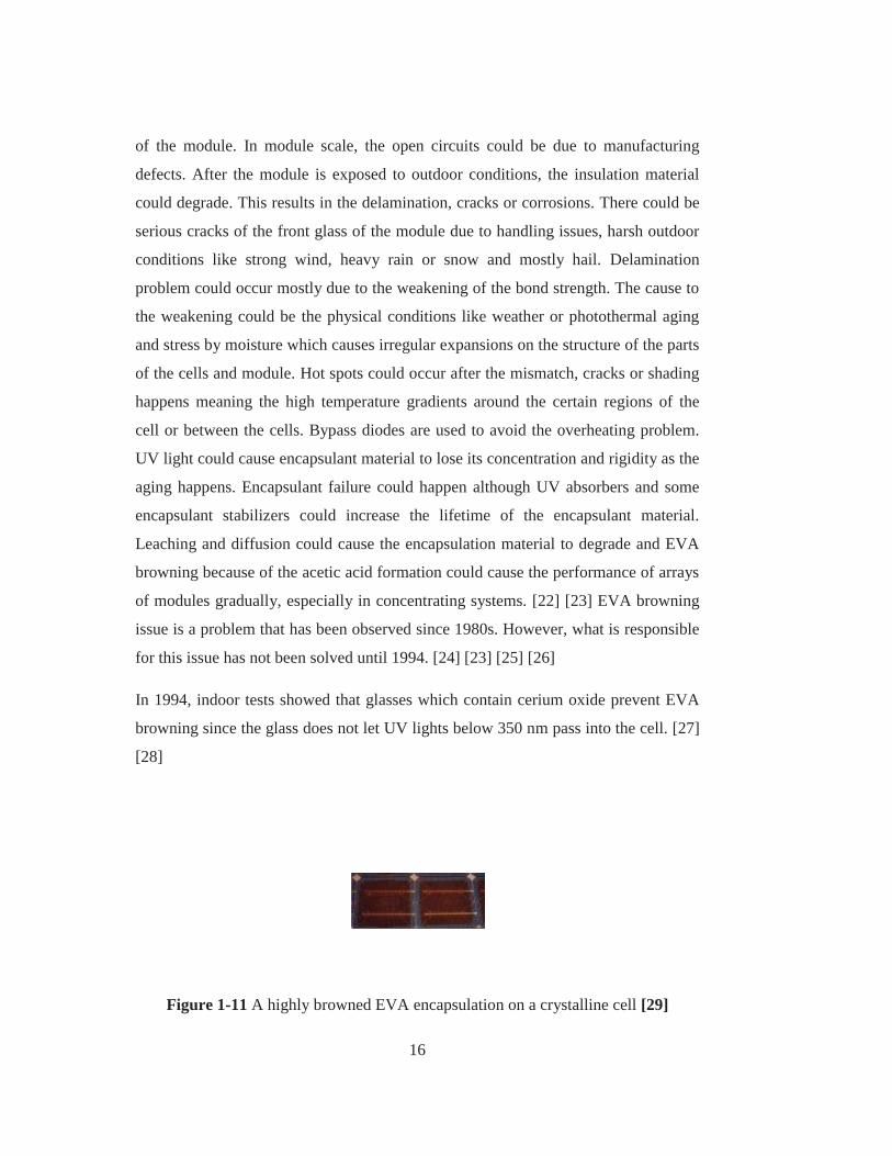
for this issue has not been solved until 1994. [24] [23] [25] [26]
In 1994, indoor tests showed that glasses which contain cerium oxide prevent EVA
browning since the glass does not let UV lights below 350 nm pass into the cell. [27]
[28]
Figure 1-11 A highly browned EVA encapsulation on a crystalline cell [29]

17
When the cell or module is exposed to UV light, it causes corrosion in solder bonds
and electrical contacts. [30] [31] [32] This also increases the leakage current. [33]
A PV cell consists of materials of four different kinds in general: glass, metals,
polymers and semiconductor. Front cover of a PV cell is made of glass while the
frame is generally metal, encapsulation material is a polymer and the solar cell itself
consists of a semiconductor. Back sheet of the module is often a polymer or glass.
Junction box could be a metal or polymer while cables, string connectors consist of
metals.
Figure 1-12 An example of layers of a photovoltaic module [34]
Figure 1-13 Encapsulation of a PV module [35]

18
Mostly observed physical failure modes could be categorized as [36]:
Encapsulant and back sheet browning or yellowing
Delamination of encapsulant and backsheet
Bubbling
Busbar oxidation
Busbar discoloration
Connection corrosion
Back sheet cracking
Formation of hot spots and regions
Breakage of cells
Micro cracks
Figure 1-14 Failure modes of PV modules caused by packaging material and
detection methods

19
In almost all cases, the main cause of the physical degradation is temperature,
humidity, water penetration or UV light intensity.
1.2.2. Physical Degradation Modes
Lanoy and Procaccia (2005) described the degradation as the gradual deterioration of
the characteristics of a component or of a system which may affect its ability to
operate within the limits of acceptability criteria and which are caused by the
operating conditions. When a PV module degrades, it still could operate, but not in
the optimal values. After the module degraded for a certain rate (around 20%),
module performance could create problems (Charki et. al, 2012). Numerically, a PV
module is counted as degraded if it performs 80% of its initial power value.
(Wohlgemuth et. al 2005). Physical degradation on PV modules could be categorized
under four main subtitles[37]:
1.2.2.1. Corrosion
The main cause behind the corrosion is the moisture. [38]
Corrosion badly affects the metallic parts of the module causing the leakage currents.
It also harms the adhesive surface between the metallic frame and the cell itself. [39]
According the accelerated tests that Wohlgemuth and Kurtz conducted, after 1000 h
of exposure to 85% humidity and temperature of 85°C, corrosion started to be visible
to the eye. Wohlgemuth et al. at 2005 also claimed that the corrosion is the most
common way of physical degradation mode in solar modules. Many other scientists
in the literature proved that the corrosion is the most commonly encountered
degradation mode along with the discoloration and the main reason behind this
phenomenon is said to be the sodium in the structure of the cell that could interact
with the moisture content. [40]
It is also indicated that the faster forms of corrosion could be due to the oxygen
between the silicon junctions of the crystalline modules. [41]
Especially in humid and hot geographies, it is even more important to avoid the
moisture penetrate into the cell because there happens to be faster diffusion of water

20
into the ethylene vinyl acetate (EVA) and it could decrease the lifetime of the cell
significantly. It is also suggested in the literature that the only way to avoid this
faster penetration is sealing the cell by using gaskets with low diffusivity thanks to
the big amount of dessicant in them. [38]
Figure 1-15 Visible corrosion at the edge of the cell
1.2.2.2. Discoloration
Discoloration results in degradation in Ethylene Vinyl Acetate (EVA) or adhesive
material between the glass and the PV cells. It is basically the color change generally
to yellow or brown. This change affects the transmitted light into the cell and
decreases the module power. [42]
The most effective cause for this kind of EVA degradation is found to be the UV
lights with water at high temperatures (>50°C). Discoloration could be seen at the
different regions of the cell due to the different characteristics of the polymer
material. This also proves that the discoloration phenomenon is resulted from the
material of encapsulation instead of EVA itself. [43]
In an experimental work, which include artificial radiation exposure of a solar
module in order to investigate the UV effects on the degradation (between 280 nm
and 380 nm wavelengths) under 4000 W/m2. A very fast degradation in PV cell
performance is observed. In addition to that, a discolouring of EVA layer causing PV

21
performance loss is seen after 400h of exposure time. When the conditions are
changed to 1000 W/m2 and 500 h, the same effects are not seen on the UV region.
[44]
Another experimental study shows that for the UV region, the discoloration only
occurs under 15 kWh/m2 global irradiation between the wavelengths of 280 and 385
nm at 60 °C temperature. [45]
Discoloration of the cell has been studied experimentally and it is found that
detrimental effect on short-circuit current is around 6-8% for the partial discoloration
and up to 13% for the total discoloration. Maximum power of the module is also
decreased around 5%. [46] [30] [33]
Figure 1-16 Discoloured solar cell [47]
1.2.2.3. Glass soiling:
Glass soiling is another physical degradation mode that could be seen by naked eye
as a darkening or haziness on the cell surface, mostly on the low edges of PV module.
Glass soiling is not the accumulation of dirt on the surface of the module. It is more

22
related to the particles from air, accumulation of the remains of rain water or the ion
exchange between the glass and hydrogen ions in the water. [48]
The glass soiling could worsen under the polluted air conditions along with the use
of frames since they could allow some water to accumulate on them. This results in a
loss in optical performance (low optical transmittance) of the cell.
Figure 1-17 Haziness that could be seen at the edge of the cell
1.2.2.4. Delamination
This degradation mode occurs between the cell and the front glass or encapsulating
material. Delamination mainly has two degrading effects. Firstly, it allows light to
reflect more and water to penetrate in higher amounts into the cell. [39]
Delamination is stated to be more harmful if it occurs at the edges of the module
because it could both cause power loss and electrical risks for the whole installation.
[49] Delamination problem also occurs more in humid and hot climatic conditions
and it could cause metal corrosion problems due to the moisture penetration. It is also
claimed that the delamination occurs because of the accumulated salt and penetrated
moisture into the cell and the connection between them is formed by the hydrofluoric
acid formed by the tin oxide and fluorine both of which are present in the structure of
the PV cell. [50]

23
Figure 1-18 Delaminated photovoltaic module [47]
1.2.2.4.1. Front- side delamination:
A white milky color could be observed at the cell perimeter and the interconnection
ribbons. This problem is generally caused by the delamination of EVA and is
originated by the chemical reaction between anti – reflective coating and additive
materials in the encapsulant. The region of the occurrence of this degradation is
almost always at the same points namely; around cell busbars and perimeter of the
cell mostly due to these places having lower thicknesses than other parts of the
module. [51]
1.2.2.4.2. Front grid and AR coating:
The loss of adhesives between the cell and the encapsulant could cause oxidation and
corrosion on anti – reflective layer as well as metallic parts of the cell. The
degradation on the AR coating could be observed as a darkening on the central
region of the cell due to the oxidation. The darkening starts at the center and moves
towards the edges as could be seen in the Figure 1-20 below. Anti-reflective coating
is used to decrease the reflectivity of the silicon along with the texturing. At the
highest intensity of solar spectrum 600 nm, reflection rate of the silicon is 35%.
Texturing and anti-reflective coating (AR) decreases this rate around 23%. [52] Open
circuit voltage and short circuit current increase as the rate of reflectivity decreases.
This increases the overall power of the cell significantly. AR coatings are transparent

24
and generally made of oxides. The degradation in AR coatings could result in
decreased current, therefore decreased power because it absorbs less photons and
could be caused by the inter-diffusion from the contents of the emitter region.
Degradation in AR coating could be visibly observed as the brightened color of the
cell or by measuring the open circuit voltage and short circuit current. [53]
1.2.2.4.3. Bubbles:
This mode of degradation has the similarity with the delamination in EVA, but in
bubbling the degradation occurs in a smaller area and causes the surface swelling
along with the loss of adhesive material as in delamination. The main cause for the
bubbles to form is the chemical reactions happening in the cell resulting in gas
emission and those gases accumulate in the cell. Bubbles could be formed on the
back of the module making it difficult for cells to dissipate the heat on them,
therefore resulting in overheating and decreasing their performance and lifetime.
Figure 1-19 below shows a monocrystalline PV cell with bubbles formed on the back
side. [54]
Figure 1-19 A PV module with bubbles on the back side [39]
Bubbles frequently appear towards the center of the cell because they are mainly
caused by the lack of adhesion which is caused by the overheating. If the bubbles are
formed on the front side of the cell, they block the radiation absorbed by the cell and
causes increased reflection of the light which reduces the power of the cell. [39]

25
Figure 1-20 AR coating oxidation through the center of the cell
The reason could be explained with the humidity accumulation since EVA is a
copolymer that could allow the diffusion of water vapour and oxygen very easily.
Therefore, it also could let the oxidation move around in an easier way. [51]
It is also suggested in the literature that ‘breathable’ parts like edges are less affected
by acidic acid because the humidity could escape to the outside of the cell easily in
those areas. [55]
1.2.2.5. Breakage and cracking cells
Breakage of the cell is an important degradation mode. It could occur during the
transportation, maintenance or installation of the cell. [45]
Cells could still function for a long time without any problems despite the cracks on
them, but there could always be electrical shock and water ingress risks after the
breaks occurred. Cell breakage may not be a degradation mode that could drastically
decrease the performance of the cell by itself, however it is mostly followed by the
corrosion, discoloration and delamination and they could cause severe power cuts.
[56]
In order to cut the production costs and raw material saving, PV manufacturers are
altering the thickness and the surface of the cell recently. For instance, cell thickness

26
is reduced under 200 μm from 300 μm and in some cases, it could be manufactured
under 100 μm. also, the dimensions of the surface of the cell are increased to 210
mm for both sides. [57] This renewals decreases production cost of the cells, but
increases the risk of breaks. Generally, these breaks could not be seen by naked eye
unless there is high damage on the module, optical methods are used to detect them.
1.2.2.6. Potential Induced Degradation (PID)
Cells are connected in series to form modules with the necessary amount of voltage
that could reach up to several hundreds. Normally, all the metallic parts in the PV
module are grounded in order to avoid electrical shocks, but it is possible to have
some leaking electrons from the parts of the module because of the potential
difference between the structure and PV module itself and bad insulation between the
structure and the layers of the cell. The performance of the PV cell degrades by this
inside polarization. This is known as Potential Induced Degradation (PID) and it
causes a gradual performance cut in the module in time because of the induced
electrical current in the module. [58]
Figure 1-21 Severely broken glass on a polycrystalline PV module [59]
Experimental works show that PID is more commonly encountered in humid
environments too along with the corrosion and discoloration meaning that leaked
current increases with the increased humidity. [60]

27
1.2.2.7. Hot spots
This failure mode results in very high temperatures in a small area in the module that
could cause damage and performance loss or failure in the module. Hot spots are
mainly caused by the failures or mismatch of the cells, shadowing or the problems in
the interconnections between the cells of a module. [61] Short circuits cause cells to
have negative and reversed value of the actual cell. This leads to a load in the
connected cells in series and makes that cell with the defect be more vulnerable for
the formation of hot spots. [62]
Figure 1-22 Hot spot formation
1.2.2.8. Mismatched Cells
Many other degradation modes could result in mismatched cells like AR coating
degradation, manufacturing defects, cracking or shadowing of the cell, encapsulant
deterioration. Cell mismatching is harmful for the cell lifetime and performance
because in a series connected cell system, if one of the cells produces lower current
than the other cells in the module, other cells act to reverse bias the defected cell.
This causes the degraded cell to dissipate power in the mode of heat. Busbars in the
cell structure are used to avoid this situation. [63]

28
Figure 1-23 Busbars help prevent the cracked cell producing lower current (a)crack
removing the part of the cell from the circuit (b)
High temperatures in the mismatched cells could cause delamination over 150°C. [63]
Mismatched cells could cause cell breakdown if the reverse bias rate is higher than
the highest voltage that the cell could endure. In addition to that, hot spots on a cell
in the module not only decrease the efficiency, but also affects fill factor badly due to
lowering the open circuit voltage and short circuit current. Bypass diodes are used to
avoid permanent hot spot formation. Mismatched cells could be observed by visual
observation, temperature monitoring of the cells and the module or by I-V curve
measurements.
1.2.2.9. Temperature Induced Degradation
Power of a PV module at standard test conditions (1000 W/m2 irradiance and TCell =
25 °C and Air mass 1.5 global spectrum) is one of the most important specialty.
However, when the module is operating at outdoor conditions, 15% of the incident
energy could be converted to the electricity. The remaining energy is mainly
converted to heat or reflected back from the glass surface or from the cell. Therefore,
an average value of the temperature for a module is almost always higher from 25°C.
higher temperatures make the bandgap of the cell decrease which allows longer

29
wavelength photons to be absorbed. Also, minority carrier lifetime increases by this
temperature increase and this will give a boost to the short circuit current of the
module. On the other hand, this will decrease the saturation current of the module
exponentially. [64]
Consequently, open circuit voltage of the cell decreases. Since the decrease of open
circuit voltage is exponential, therefore higher than the increase in short circuit
current, overall efficiency and fill factor is going to be diminished with the increased
temperature. [21]
Statistics show that the physical degradation on crystalline PV cells could be broken
down as in the Table 1.4.
Table 1-4 Physical Degradation Modes Breakdown [65]
Physical Degradation
Mode
Percent
(%)
Delamination 42
Corrosion 19
Breaking 19
Discoloration 12
Ribbon Crack 8

30
Table 1-5 Thin-film failure modes and mechanisms [66]
Failure Modes Effect on I-V curve Possible failure
mechanisms
1. Cell Degradation
a. Main junction:
increased
recombination
Loss in fill factor, ISC
and VOC
Diffusion of dopants,
impurities etc.
Electromigration
b. Back barrier, loss of
ohmic contact (CdTe)
Roll-over, cross-over
of dark and light I-V,
higher RSeries
Diffusion of dopants,
impurities etc.
Corrosion, oxidation
Electromigration
c. Shunting RShunt decreases Diffusion of metals,
impurities etc.
d. Series; ZnO, Al RSeries increases Corrosion, diffusion
e. De-adhesion SnO2
from soda-lime glass
ISC decreases and
RSeries increases
Na ion migration to
SnO2 /glass interface
f. De-adhesion of back
metal contact ISC decreases Lamination stresses
2. Module degradation
Interconnect
degradation
a. Interconnect
resistance; ZnO:Al/Mo
or Mo, Al interconnect
RSeries increases Corrosion,
electromigration
b. Shunting; Mo across
isolation scribe RShunt decreases
Corrosion,
electromigration
Busbar degradation RSeries increases or
open circuit
Corrosion,
electromigration
Solder joint RSeries increases or
open circuit
Fatigue, coarsening
(alloy segregation)

31
Table 1.5 (cont’d)
Failure Modes Effect on I-V curve Possible failure
mechanisms
Encapsulation failure
a. Delamination Loss in fill-factor, ISC,
and possible open circuit
Surface contamination,
UV degradation,
hydrolysis of silane/glass
bond, warped glass,
‘dinged’ glass edges,
thermal expansion
mismatch
b. Loss of hermetic seal
c. Glass breakage
d. Loss of high-
potential isolation
1.2.3. Light Induced Degradation
This degradation mode is also known as the Staebler – Wronski effect which is a
very common problem that is encountered in a-Si cells. [67] When the module is
exposed to light, electron hole pairs are produced and recombined. The energy
produced during this recombination process could break the weak Si-Si bonds in the
structure of the cell causing meta - stable defect sites. These defects deteriorates the
PV cell material therefore causes performance cut in the module. [68] Light induced
degradation could be observed by periodic measurements of the ISC and VOC. [53]
In amorphous silicon technology, light induced degradation could cause ~10 – 30%
efficiency loss in the first several hundred hours of light soaking. According to
Staebler – Wronski effect (SWE), conductivity (both dark and photoconductivity) of
hydrogenated amorphous silicon decreases when it is exposed to light. However, it
32
could be reversed by annealing over 150 °C. Mechanism of the SWE could be
summarized as the recombination – induced breaking of weak Si – Si bonds by
optically excited carriers after thermalization resulting in defect centers that lower
career lifetime.
Literature has many proposed mechanism for the SWE, however exact mechanism
could not still been understood thoroughly. However, it is proven that the SWE is
not affected by the impurities. [69] The degradation occurs in the bulk material with
a contribution from the surface.[70] The accelerated test of the effect is proven to be
possible by using high intensity pulsed light at the standard operating temperature.
[71] Effect of the annealing process is explained with hydrogen diffusion.
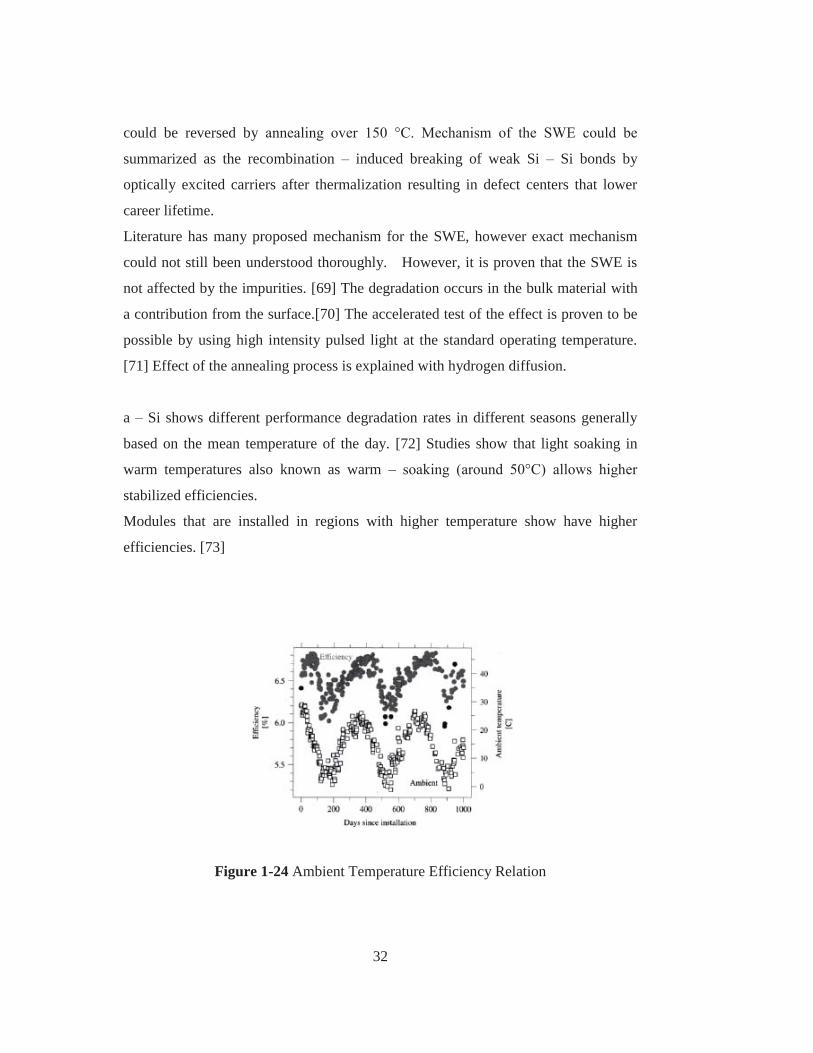
a – Si shows different performance degradation rates in different seasons generally
based on the mean temperature of the day. [72] Studies show that light soaking in
warm temperatures also known as warm – soaking (around 50°C) allows higher
stabilized efficiencies.
Modules that are installed in regions with higher temperature show have higher
efficiencies. [73]
Figure 1-24 Ambient Temperature Efficiency Relation

33
This 10 – 15 % change is mainly due to the annealing on the defects caused by SWE.
Therefore, temperature is an important parameter for the degradation due to light
soaking and the stabilized efficiency of the cell depends on the temperature during
light – soaking atmosphere. [74]
Mostly observed degradation mechanisms in other thin film technologies are on
CdTe and CIGs cells. In CdTe cells, the degradation is related with the copper in the
cell. Since the p – type CdTe could not be contacted with the metal, copper is added
to the structure before making the contact. [75] [76] Copper in the structure could
affect the electrical properties of CdTe cell dramatically because the copper is very
mobile in the structure and it can move to the grain boundaries of the cell to create
recombination centers near the p – n junction region. Therefore, even low amounts of
copper could decrease the electrical properties of the cell. In addition to that, the
electric field causing the applied voltage either external or in the cell could make
copper ions move towards the front contact and it is known from the literature from
the experiments of the accelerated aging tests that the CdTe degradation is affected
by the open – circuit conditions like this. [77] Also, it is known that the impurity
diffusion and change in doping material (Cu in this case) could cause instabilities in
the performance of the cell. [78] [79]
In CdTe technology, the cell structure could be summarized as TCO /n – CdS / p –
CdTe / back – contact . [80] The main problem for CdTe modules is the back sheet
metallization and it requires high work function for ohmic contact. Studies show that
Te – rich interfacial layer could be beneficial to lower the metallization. [81] [82]
Using Cu is beneficial; however its high diffusivity causes stability problems.
Studies show that high temperatures increase the rate of degradation in the cell and
the module for CdTe technology. [83]Tests on CdTe cells manufactured with
different recipes show no significant difference in efficiency at light soaking.
Therefore, it is stated that for the accurate determination of the efficiency, long term
test are needed (at least >5000 hours of light soaking). [77]

34
Figure 1-25 Electric Field for the Layers of CdTe Cells
Figure 1-26 Efficiency vs Time at Different Temperatures for a CdTe Cell

35
Back contact in CdTe technology could create reverse polarization resulting
degradation in performance. Cu is added to lower this polarization and increase I and
V performance. [84]
Figure 1-27 Effect of Cu Addition
At high temperatures, Cu at the back side is lost and diffused through the cell and
this causes decrease in fill factor of the module.
Figure 1-28 Suggested Mechanism of Cu Diffusion

36
For CIGS technology, due to its flexible structure, copper is said not to affect the
stability of the cells. [85] More importantly, heat tests shows that humidity is a more
obvious cause for the performance degradation (VOC and FF reduction) since it
causes an increase in the deep acceptor states concentration in the CIGS absorber.
[86]. In CIGS technology, there are two different configurations for the deposition
of the cell.
CIGS modules are typically formed in substrate configuration. When they are formed
in superstrate form, undesired CdS diffusion could be a problem during the
deposition process.
In reversible metastability conditions for CIGS cells, annealing at 80 °C doubling the
decrease in the conductivity in dark when compared to the conductivity at room
temperature. [87] When the cells are exposed to light, initial state is provided again.
VOC of CIGS cells could shift reversibly with light exposure. Light exposure could
increase VOC by 5% and this effect could be fastened by increasing the temperature.
[88]
Figure 1-29 CIGS Cross - Section

37
Other degradation causes could be categorized as the effect of Ga content on the cell
stability and donor type defects. [89] [90] According to the simulation, thinner cells
show reduced LID degradation. [91]
1.3. Performance Characterization Studies – Outdoor Testing Stations
1.3.1. PV Module I – V Characteristics
A solar cell could be modeled as a single diode with all the internal resistances in the
system.
Figure 1-30 Single diode model of a PV cell
Dark and light I – V curve measurements are made to understand the electrical
performances of a solar module. The dark I – V measurements result in:
(1. 1)
ID represents the dark current as I0 is reverse saturation current, q is the charge of the
electron, k is Boltzmann constant and T is the temperature.
In illuminated conditions, the characteristic equation for the solar cell becomes:
(1. 2)

38
IPH represents the current under that the light has produced, a represents the diode
factor.
the above equation is valid for a solar cell, but not for a complete module since a
solar module consists of 28 to 36 solar cells connected in series. Therefore, different
parameters and variables should be added into these equations in order for solar
module to be represented better. [92]
Therefore, the diode approach should be modified. Characteristics of a solar module
could be understood in a better way with the equations below:
(1. 3)
(1. 4)
By the help of this equations, the main characteristics of a PV module like short
circuit current (ISC), open circuit voltage (VOC), maximum power (PMAX), fill factor
(FF) and efficiency are determined.
PV modules are rated with their PMAX values in the market and this value is found
under the standart test conditions abbreviated as STC which is known as testing
under 1000 W/m2 solar radiation, 25°C of module temperature and at air mass 1.5g.
Determination of this PMAX value is known as the characterization of the PV module
and this procedure is done with the solar simulators. After the characterization, PV
module is labeled with the VOC, ISC, VMAX, IMAX and PMAX.
However, these STC parameters are not very similar to the real conditions that the
solar module will mostly be exposed. The sun will not always provide 1000 W/m2
and the module will probably have a temperature of higher than 25°C because of the
weather conditions and outdoor factors. Consequently, a solar module will almost

39
always perform below the labeled values of power, voltage and current. Therefore,
other test conditions are used to have more realistic perspective about the module.
These are standard operating conditions (SOC) and nominal operating conditions
(NOC). These two approaches use nominal operating cell temperature (NOCT)
concept. NOCT is defined as the open circuited cell that is exposed to irradiation of
800 W/m2, 20 °C and 1m/s wind speed. Under these parameters, NOCT value is
around 40 to 50 °C. Three different approaches are tabulated below:
Table 1-6 STC, SOC and NOC Definitions
Conditions Standard Test
Conditions (STC)
Standard
Operating
Conditions (SOC)
Nominal
Operating
Conditions
(NOC)
Irradiation
(W/m2)
1000 1000 800
Temperature
(°C)
25 NOCT NOCT
Wind speed
(m/s)
- 1 1
There are various factors that are affecting the performances of the solar modules.
Studies show that these factors could be categorized under five subtopics namely the
technology of PV module, temperature, irradiation, tilt angle and others.
1.3.2. Effect of the type of PV technology
The main factor that is changing the performance of a PV module in terms of the
technology is the efficiency. Mono crystalline PV modules have higher efficiencies
(around 15 – 18%) compared to the other commercialized technologies such as poly
40
crystalline and thin film cells, but mono crystalline PV modules are more
complicated to produce and causing high costs. On the other hand, poly crystalline
modules are easier to produce with a cheaper price and having lower efficiencies
around 8 to 12%. [93] [94]
Amorphous silicon cells have efficiencies around 5 – 7% while CdTe and CIS
technologies provide efficiencies of 16 and 20%. [95] [96]
Technology creates the basis and the upper limits for the efficiency of the solar
module; therefore it is always the major affecting factor.
1.3.3. Ambient temperature
The performance of the module is dependent to its temperature, but the module
temperature is also dependent to the ambient temperature. Module temperature is
higher than the ambient temperature because the glass frame of the module absorbs
the infrared part of the sunlight and encloses the heat. This increase in module
temperature decreases the band gap of the cell. [92]
This increases the ISC of the cell, but decreases VOC and the decrease in VOC
overcomes the increase and affecting the power negatively. Therefore, the power of
the module decreases if the operating temperature of the module increases.
Monocrystalline PV cells are affected greater than the other technologies. Studies
show that 15 % of a performance cut could be seen on monocrystalline modules as
this figure is around 5% in amorphous PV cells. [97]
Increasing temperature decreases efficiency and power to minimum at stagnation
temperature and it could also create physical problems like hot spots, degradation in
wires or encapsulant. [98]
1.3.4. Solar Irradiation
Solar irradiation has a linear relationship with the power of the module. Higher solar
irradiation provides more incident photons for to activate the electrons in the
structure of the solar cell meaning more electricity production. However, studies also
show that different PV technologies have different responses to increasing irradiation.

41
For instance; Eikelboom and Jansen states that monocrystalline modules show no
power cut under outdoor irradiation. However, CIS and amorphous silicon cells show
major degradation in terms of power at STC. The study was made with nine different
types of PV modules. The final results also show that thin film technology modules
perform better under low irradiation. [99]
1.3.5. Tilt Angle
The performance of a PV module depends on the radiation amount that it is receiving
during the day time and this amount is dependent on the tilt angle and orientation of
the solar module. [100] [101]
The orientation of the solar module is generally the south for the places in Northern
hemisphere and north in the Southern hemisphere. However, tilt angle is dependent
on where the module is installed and must be optimized accordingly. There are
different methods for optimizing the tilt angle from computational calculations to
tracking devices for the best orientation during the daytime. [102]
Each of them differs in terms of the site that PV modules are installed.
1.3.6. Others
Four factors mentioned above have significant effects on performance. However, the
variables in the other section are still affecting the power of the module, but in a
lower extent. Other factors could be like accumulation of the dust, humidity, wind.
1.3.7. Evaluation of the PV Performance
In order to standardize the quality of PV modules, it is needed to develop some
parameters that are universally acceptable and representing the specialties of the
modules thoroughly. Therefore, International Electro – technical Commission has
developed these mentioned parameters in order to rate and analyze the performances
of the solar cells under different operation conditions with different technologies.
[103]
These standardized parameters are needed for three main reasons:

42
A set of parameter is needed to label and express the modules operating with
different technologies and at different geographies, times of the year and designs
on the same basis.
These parameters should also express the losses on the module.
Decided parameters should also help designers for validating the models for
system characterization of a single module or an array of modules.
There are mainly four parameters that could be used for the evaluation of the PV
module performance:
1.3.7.1. Final yield (YF)
Final yield defines the ratio of total energy that is produced by the system during a
specified time interval to the rated power generation. Rated power generation implies
the amount of energy that the system could produce under STC. To formulate:
(1. 5)
E stands for the amount of energy that is produced by the system in a specified time
interval and PPV,Rated is for rated power.
1.3.7.2. Reference Yield (YR)
Reference yield is denoted as solar radiation divided by the reference solar radiation.
The time interval is the same for the two radiation units.
(1. 6) Ht: total solar radiation (kW h/m2)
G: reference irradiance (1 kW/m2)

43
1.3.7.3. Performance Ratio
Performance ratio is calculated by dividing the final yield to the reference yield.
This property is a dimensionless variable that is expressing the normalized
performance of the solar module. In addition to that, it gives information about the
rate of losses in the module therefore widely used in the long term evaluation of the
solar cells. Generally, decreasing values of performance ratio along the years makes
it possible to see the degradation rate on the system.
(1. 7)
1.3.7.4. PVUSA Rating
PVUSA rating method is used to calculate the performance of the PV module by
regressing the meteorological data from the site that the system is located. The data is
calculated at the PVUSA Test Conditions (PTC) which are 1000 W/m2 irradiance,
20°C temperature and wind speed of 1 m/s. In PVUSA, the power output depends on
those three variables.
(1. 8)
P: the power output in kW
E: amount of irradiance in W/m2
Ta: ambient temperature in °C
WS: wind speed in m/s
A & D are the regression data calculated from the experimental data

44
1.3.7.5. Capacity Factor (CF)
Capacity factor is the ratio of the annual power production amount (EAC,a) to the full
rated power amount of the system (PPV,rated) for the same period of time.
(1. 9)
1.3.7.6. System Efficiency
System efficiency is defined as the produced energy divided by the irradiation
amount multiplied with the module area for a specified period of time (a month for
the formula below).
(1. 10)
ηsys,m stands for the monthly efficiency
EAC,D stands for the energy produced by the system
Ht stands for the amount of irradiance
Aa stands for the module area [104]
1.3.8. Outdoor Studies
The outdoor studies aiming to monitor PV technologies over long period of time in
order to characterize the performance and degradation modes are listed below:
In the first study, Ayompe et al. measured the performance of a roof PV system in
Ireland, Dublin for eleven months from November 2008 and October 2009. The PV
system consists of monocrystalline silicon modules with peak power value of 215
watt each and 17.2% efficiency. Performances of the PV cells are monitored on
monthly and yearly basis along with the seasonal variations. The annual final yield
value is calculated as 2.4 kWh / kWp-d. [105]

45
Work of Emmanuel et al. monitored a PV system on grid with a 171.36 kWp
power at Crete, Greece. The PV system is monitored for a year’s time starting from
2002 and the power loss modes resulting from temperature, soiling, grid based
problems are also calculated in this study. The final yield is reported as between 1.96
and 5.07 h/d and performance ratio is changed around 58 to 73% resulting in an
average PR of 67.36%. [106]
Work of Pietruszko et al. consists of 20 double junction thin film modules with a
total power of 1 kWp panels installed at Warsaw, Poland in 2000. The performance
of the system is evaluated one year later and the after eight years’ operation in 2008.
It is indicated that the system provided power value of 830 kWh for the first year’s
operation which is more than the expected power of the computer simulation in the
study. The performance ratio of the system is changing between 0.6 and 0.8 in the
first year. For the first three years’ operation, performance ratio values are ranging
from 0.52 to 0.6, showing a decreasing trend because of the thin film stabilization
issue. This work also includes the effects of meteorological parameters and
irradiance, temperature and tilt angle with an AC and DC voltage analysis. [107]
[108]
Soa et al. monitored and evaluated the performance of four arrays of 3 kW grid
connected PV system consisting of two multicrystalline and two monocrystalline
groups. The PV arrays are monitored for one year and the system is also simulated
with PVSYST software by using the measured data. Performance ratio values are
ranging between 76.8 and 78.1% for third and fourth arrays. However, there is
performance loss of 14% because of degradation in the modules and mismatch
between sub arrays in first and second arrays even though all are installed in the
same way. Final simulation depending on the measured values showed that the whole
system performance could be improved up to 13%. [109]
Sharma and Chandel worked on a PV on grid system of 190 kWp capacity located
in India for one year’s time. The range or final yield, reference yield and
performance ratio are 1.45 – 2.84 kWh/kWp-d, 2.29 – 3.53 kWh/kWp-d, 55 – 83%

46
respectively. Performance ratio in the average of nine years is found to be 74%. It is
also stated in the publication that the tilt angle must be optimized for better power
production. [110]
Makrides et al. established outdoor stations at three different locations Cyprus,
Nicosia and Stuttgart. These systems have 13 different kinds of PV technologies with
a grid connection and capacity of 1 kWp. Power production values for the Cyprus,
Stuttgart and Nicosia are 1600 – 1700, 1194, 1580 kWh/kWp, respectively. Power
amount is higher in the system located in Cyprus because of the average irradiance
amount of Cyprus is more than Stuttgart and Nicosia. In addition to that, the highest
ambient temperature between three locations is at the Cyprus climate (module
temperature is around 60°C). This study reveals that the PV modules having a lower
maximum power to temperature coefficient ratio (PMPP % / K) are producing higher
performances in terms energy production postulating loss of heat from the modules
in hot climates as an important parameter on module performance. [111]
Adhikari et al. tested a 45 moduled system of a total power of 2.88 kWp in a
residential place in Bangkok, Thailand. The PV system consists of 4 arrays with a
total area of 45.2 m2. The system is tested for one year’s time between 1998 and
1999 and recorded output power values, efficiency of the system, reference and final
yield along with the array yield and performance ratio. Final yield for the system is
found to be 1166 kWh/kWp and the highest yield value is found at June as 129
kWh/kWp with the total system efficiency of 5.4%. [112]
Ruther et al. studied on a 2kWp double junction a – Si building integrated photo
voltaic (BIPV) grid connected system in Brazil. Performance ratio of the system is
found as 82% for AC and 92% for DC after 5 years of operation. It is indicated in
this study that after the evaluation of performance, it is seen that once the
stabilization period is over for a – Si solar modules, the performance becomes
independent from the operating temperature. Therefore, it is more convenient to use
this kind of a system in warm climates for better performance. [113]

47
Studies above show that there are many parameters like geography, technology,
system design, orientation that could differ PV systems and arrays from each other
and performance evaluation parameters like performance ratio (PR) or final yield (YF)
are very useful to put them into a common basis for comparison. In addition to that,
performance evaluation parameters make it possible to observe the effects of
degradation and aging losses numerically. Those measurements and metrics also
provide information on which degradation mode (other than time) could be dominant
in the system. It is also clear that the PV modules individually should be tracked
since they are the most important parts of this integrated systems along with their
utilities for power production and degradation modes should be fully understand in
order to increase the cell, module and system life and efficiency.
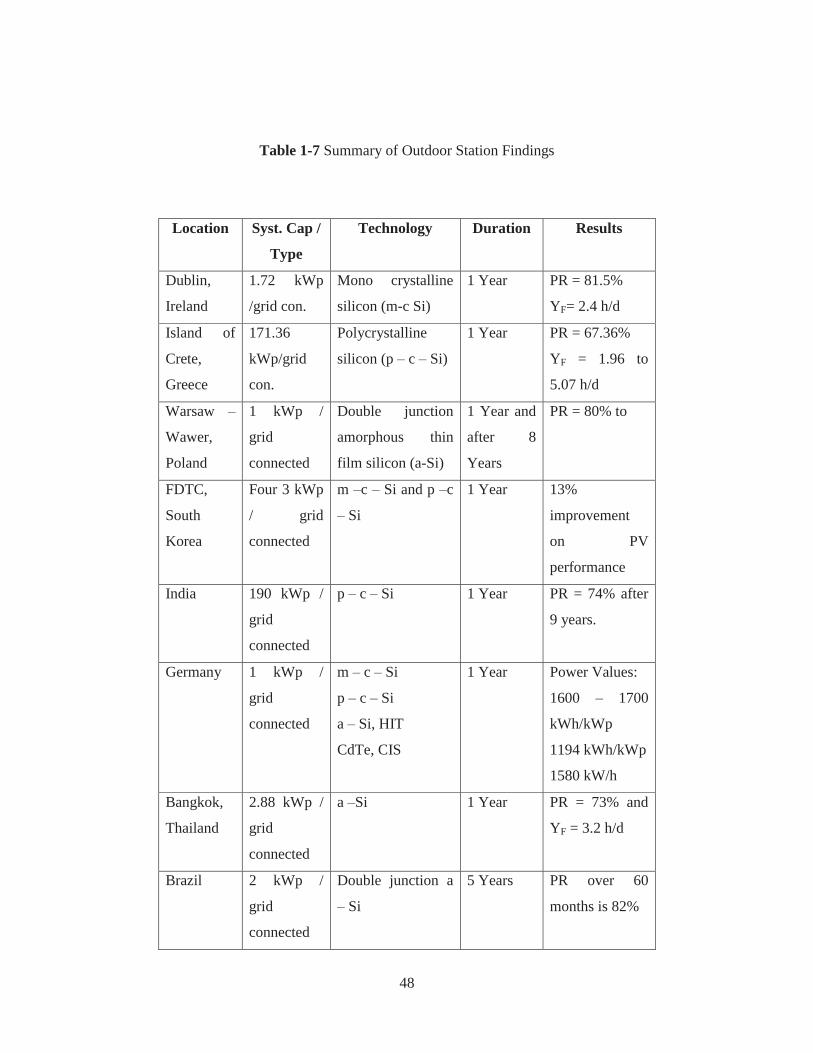
48
Table 1-7 Summary of Outdoor Station Findings
Location Syst. Cap /
Type
Technology Duration Results
Dublin,
Ireland
1.72 kWp
/grid con.
Mono crystalline
silicon (m-c Si)
1 Year PR = 81.5%
YF= 2.4 h/d
Island of
Crete,
Greece
171.36
kWp/grid
con.
Polycrystalline
silicon (p – c – Si)
1 Year PR = 67.36%
YF = 1.96 to
5.07 h/d
Warsaw –
Wawer,
Poland
1 kWp /
grid
connected
Double junction
amorphous thin
film silicon (a-Si)
1 Year and
after 8
Years
PR = 80% to
FDTC,
South
Korea
Four 3 kWp
/ grid
connected
m –c – Si and p –c
– Si
1 Year 13%
improvement
on PV
performance
India 190 kWp /
grid
connected
p – c – Si 1 Year PR = 74% after
9 years.
Germany 1 kWp /
grid
connected
m – c – Si
p – c – Si
a – Si, HIT
CdTe, CIS
1 Year Power Values:
1600 – 1700
kWh/kWp
1194 kWh/kWp
1580 kW/h
Bangkok,
Thailand
2.88 kWp /
grid
connected
a –Si 1 Year PR = 73% and
YF = 3.2 h/d
Brazil 2 kWp /
grid
connected
Double junction a
– Si
5 Years PR over 60
months is 82%

49
1.4. Accelerated Testing in Light Soaking Station
The main logic behind the accelerated testing for PV modules is the need for quicker
data and judgments than the real – time tests. In an outdoor station, the modules are
tested every day with periodical data measurements under the real weather conditions
for a long time, generally not less than one year because the amount of time is
basically needed to see the trends of the equipment for different weather conditions
and seasonal effects along with the varying spectral conditions depending on the time
for the day. In addition to that, when the physical degradation is the thing to check, it
is an important test atmosphere to see if PV modules or cells are durable to the
geographical and environmental conditions on a specific area. Also, the indication of
the rate of degradation is another subject that provides satisfactory and real data from
an outdoor station. Accelerated tests, on the other hand are the simulated
atmospheres of the outdoor environments. Devices with the artificial light sources
are commonly used to accelerate the light induced degradation on the PV module.
These light sources could vary from filtered long arc xenon, fluorescent, metal halide
lamps and carbon arc. In some studies, mercury vapor and tungsten lamps could also
be used for light soaking testing. Accelerated testing procedure is also named as
artificial weathering.
Accelerated testing has some advantages over outdoor real – time operations. For
instance; light soaking tests could be continuously conducted under the same
conditions without considering the day – night cycles, seasonal variations or change
of weather conditions that happen unavoidably in real time testing. The parameters
like temperature, humidity or water exposure limits could be pushed over the realistic
limits in accelerated tests. For a light soaking station, depending on the power and
orientation of the lamps in the system, PV modules could be exposed to energies
multiple times more than a PV module would be exposed in a sunny day. The
accelerated test environment also provides repeatability and reproducibility in terms
of the experimentation and this is not possible in outdoor testing. Therefore, effects
of some factors could be observed individually under certain conditions.
50
Regarding the light sources, each type has its own advantages and drawbacks.
Stability of the power that is provided and the resemblance of the light source to the
actual sunlight are the most important factors when the quality is concerned.
1.4.1. Xenon Arc Lamps:
This type of lamps is first developed in 1954 and Xenon arc lamp could simulate
sunlight (UV + visible) with the most accuracy among the other lamps. Xenon arc
lamps are generally preferred when the test is wanted to be conducted under the
natural sunlight conditions. The filtering is done for the change of spectral
distribution of the lamp according to the designed experiment. Xenon arc lamps are
mainly used in the textile, paint, polymer and automotive industries. Two types of
instruments are mostly used with xenon arc lamps. One is air – cooled and the other
one is water – cooled devices. The type of cooling does not have much effect on the
spectral distribution, but they are important in terms of the design of the device and
optical filtering of the light. As all lamps do, xenon lights emit light and heat together
while radiating. Therefore, cooling is an important design parameter for the
accelerated test stations with xenon arc lamps because the filter, the lamp, the
samples that are measured or the other components of the equipment should be
protected from overheating, damages or degradation that could be caused by the heat.
This is why the two systems are called water cooled and air cooled equipments.
Neither of the cooling systems affects the spectral distribution and power amount of
the lamps. They are just for the cooling purposes.
Test equipment could have vertical or horizontal platforms for sample placing
depending on the need. Large scale equipments have two – tier and three – tier
inclined specimen racks in order to provide uniform irradiation distribution. The
racks rotate continuously around the xenon arc lamp to establish better uniformity for
irradiance, temperature, even humidity.
Xenon lamps have the closest spectral distribution to the natural sunlight in the UV
and visible range. On the other hand, in the infrared region it has significant
variations. Therefore, the xenon lamp system contains filters that could be designed
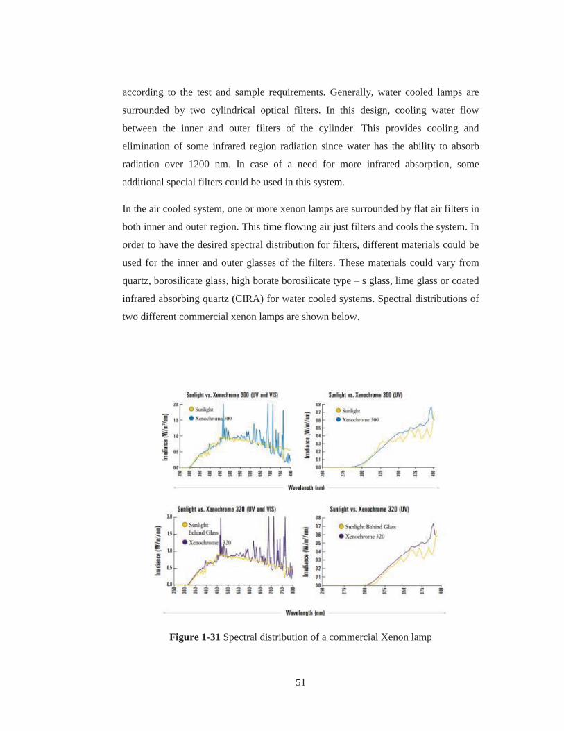
51
according to the test and sample requirements. Generally, water cooled lamps are
surrounded by two cylindrical optical filters. In this design, cooling water flow
between the inner and outer filters of the cylinder. This provides cooling and
elimination of some infrared region radiation since water has the ability to absorb
radiation over 1200 nm. In case of a need for more infrared absorption, some
additional special filters could be used in this system.
In the air cooled system, one or more xenon lamps are surrounded by flat air filters in
both inner and outer region. This time flowing air just filters and cools the system. In
order to have the desired spectral distribution for filters, different materials could be
used for the inner and outer glasses of the filters. These materials could vary from
quartz, borosilicate glass, high borate borosilicate type – s glass, lime glass or coated
infrared absorbing quartz (CIRA) for water cooled systems. Spectral distributions of
two different commercial xenon lamps are shown below.
Figure 1-31 Spectral distribution of a commercial Xenon lamp

52
Figure 1-32 Spectral distributions of a commercial Xenon lamp with different filters
Optical filtering makes it possible to control both spectral distribution and irradiance
amount for the lamp. A micro processor helps control radiant exposure. Water cooled
xenon lamps usually control the radiation at narrow wavelengths around 340 and 420
nm. Narrow band interference filters are used for this purposes and the power of the
lamp is controlled by a wattage and photodetector. On the other hand, air cooled
xenon lamp systems usually use broad band UV irradiance which is around 300 to
400 nm.
1.4.2. Fluorescent UV Lamps and Devices:
This kind of lamps have the same physical qualities with the ones that commonly
used in residential purposes, but the spectral properties of these lamps are altered to
use in light soaking systems. There are different kind of fluorescent UV lamps in

53
terms of their spectral interval and properties. One of them is fluorescent UV – B
lamps having a peak wavelength of 313 nm. Most of the energy of this lamp is
maintained between 280 to 360 nm, shorter wavelengths than the natural sunlight.
UV – B based test always reports stability values between real and accelerated
testing values since there is high amount of short wavelength UV energy and low
amount of long UV and visible radiation in UV – B lamps. This changes the light
induced degradation mechanism on the samples from outdoor test very much.
Secondly, there are fluorescence black lights also known as UV – A type lamps.
These lamps have the emission range of 340 – 370 nm and at 340 nm, the irradiance
is similar to natural sunlight behavior under 325 nm. Tests using fluorescent lamps
are widely used in light soaking practices; however test times are long compared to
other technologies and to compare between the UV – A and UV – B type lamps, tests
using UV – A lamps even last longer. However, not emitting radiation below the cut
– on of natural sunlight improves the correlation with outdoor tests for UV – A lamps.
Fluorescent lamps could be useful in terms of the ranking of materials under certain
conditions, but it is not very convenient to use them for outdoor test correlation or
performance monitoring. They are mostly used in screening tests to identify
formulation errors by testing the samples in harsh conditions. A commercial UV – A
and UV – B lamp wavelength distribution could be seen below:
Figure 1-33 Spectral distribution of UV – A&B lamps and sunlight

54
Below figure shows how the spectral distribution of a commercial UV – A lamp
resembles with the sunlight behind glass at low wavelengths. Green line represents
the commercial UV – A lamp while the yellow belongs to the sunlight behind the
glass.
Figure 1-34 UV – A vs Sunlight behind the glass
1.4.3. Metal Halide Lamps
Metal halide lamps are known for the full spectrum tests for solar simulators. The
most widely used areas are aging tests for both weathering and thermal applications.
Metal halide lamps do not have a continuous spectrum. Instead, they are the
cumulative of many individual spectrum lights that will provide a total continuum
over the wide spectrum. This is due to the rare earth metals like holmium, thulium
placed in the arc plasma of the lamp. These metals react with halogens and form
halides. Cumulative spectrum of the metal halide lamp resembles very much to the
natural sunlight. However, they have to be stabilized and controlled carefully
because variations could change this cumulative behavior drastically. Metal halide
lamps are known as discharged lamps. They have many different versions, but only

55
some of them are suitable for solar applications and daylight simulation. The most
important characteristics of the metal halide technology are the spectrum
resemblance with the natural light, stable irradiance which are very important for a
solar system.
Figure 1-35 Spectral distribution of a commercial metal halide lamp with the
sunlight spectrum

56

57
CHAPTER 2
2. EXPERIMENTAL SETUP
The experimental setup in this study aims to establish a test station that can
continuously monitor and measure the performance characteristics of installed
commercial solar panels and simultaneously measure the outdoor conditions such as
ambient temperature, pressure, humidity, wind direction and speed, solar radiation
amount along with the solar spectrum of the sun during the day. For this purpose, the
test station includes an I-V curve tracer for monitoring the performances of the
installed commercial solar modules, an outdoor weather station for the continuous
measurements of the weather parameters, mentioned above a solar
spectrophotometer for the spectral distribution of the sun and the installed solar
modules as they are the interests of all the performance characterization. The weather
station and the I – V curve tracer have their own ftp like web servers which could be
reached in and out of campus from where internet connection is available in order to
store, manage and instantly visualize the data they have been saving during the study.
On the other hand, spectrophotometer does not have its own web server, but it is
connected to a laptop that can be reached remotely any time and operating for 24
hours for saving the spectral data continuously.
Each equipment in the test station acquires different sets of data with the specified
conditions. Weather station collects the weather data such as ambient temperature,
pressure, solar radiation amount, humidity, amount of rain and wind speed and
direction. These are the values that changes according to the atmospheric conditions
during the day and night time. I – V curve tracer collects data from solar modules
installed as two different types. The first one is the I – V curves, showing the instant

58
measurements of performances of the modules with a specified time interval that
could be altered according to the measurements that are aimed to be done. Second
one is the performance data which shows the overall performances of the solar
modules during the day when they are performing at their best also known as peak
power mode. Spectrophotometer is also operating all day to collect and save the solar
spectrum data continuously with the specified conditions.
Figure 2-1 Data Acquisition Flowchart
As it can be seen from the flowchart, all collected data is stored in a computer that
can be reached from anywhere inside or outside the campus via file transfer protocol,
known as FTP server with an encrypted username and password. Actually, all of the
equipments except for the spectrophotometer have its own internal memory.
However, in order to keep the data safe from possible memory losses, low memory
conditions or unknown errors, data is also saved in different computers and in an
external memory that is updated by the new data periodically. Software called Auto
FTP Manager makes it possible to acquire the data automatically from internal
servers to the computers in desired time intervals with or without leaving the original
files in the server according to the selection of the user. Therefore, all the data could
be stored in multiple places as soon as they are put into the internal servers. That
creates confidence to prevent data from getting lost due to errors, electricity cut offs
CPU (FTP Server)
Weather Station
Atmosphere
I-V Curve Tracer
Solar Panels
Spectrophotometer
Sunlight

59
or other unknown reasons. To sum up, there are three different kinds of data from I –
V curve tracer, weather station and spectrophotometer and these data are gathered in
one computer along with the web servers of the equipments themselves.
After giving an overview of the test station and the data acquisition procedure, more
detailed information on equipments could be useful for better understanding of the
experimental setup.
2.1. HOBO U30 Station
HOBO U30 Station is a tool that makes it possible to gather instantaneous
information about weather parameters that could affect the performance and
operation of solar modules of all types. Ethernet stands for the method for reaching
the internet service of the equipment as HOBO also has GSM and wireless
connecting type models. HOBO U20 Station has different sensors that are used for
gathering different types of data from the atmosphere. Up to 15 channels of data can
be recorded and monitored remotely via web server HOBOlink. The data could be
viewed and edited via HOBOlink server specific to the station. The station that is
used in this study only has a direct internet connection with an Ethernet cable. 10
smart sensors of any type could be installed to the station in order to measure
different parameters. In this study, installed sensors could measure temperature, solar
radiation, pressure, humidity, wind speed and direction and the amount of rain.
2.1.1. U30 Station Components
2.1.1.1. HOBO U30 Ethernet Data Logger
The data logger could be thought as the main board of the station since all the sensor
slots and connection tools are inside the logger. It contains 15 channels to connect
smart sensors for measurement. The logger has its own battery for power need of the
system. This battery could be charged either by solar modules or AC power. There
are different slots for both of these energy sources. In addition to that, it has an
Ethernet cable slot to reach the HOBOlink server with periodic intervals that is set by
the user either by connecting HOBOlink via Internet or to the logger by a USB cable.
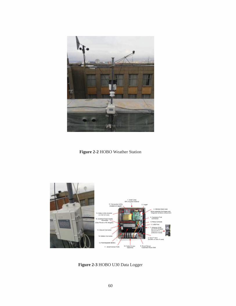
60
Figure 2-2 HOBO Weather Station
Figure 2-3 HOBO U30 Data Logger

61
2.1.1.2. Solar Radiation Sensor (Silicon Pyranometer) S – LIB – M003
Solar radiation sensor is a silicon pyranometer designed to take measurements at
outdoor conditions. All calibration parameters are stored inside the sensor. Therefore,
no additional programming or calibration is needed in order to operate the sensor.
Solar radiation sensor and all other measuring devices in this weather station are
designed in this manner. Because of this plug and measure specialties, they are called
smart sensors. As soon as the sensor is plugged into the slots in the HOBO U30 Data
Logger, they start acquiring data for the specified interval and automatically send this
data to HOBOlink server.
The silicon pyranometer has a measuring range of 0 – 1280 kW/m2 over a spectral
range of 300 to 1100 nm with a resolution of 1.25 W/m2. It can operate in rough
outdoor conditions like -40 to 75 °C temperature with an accuracy of ± 10 W/m2 or
±5%, whichever is greater in sunlight. The small cap (level) that is visible in the
figure is used for balancing purposes which makes sure that the pyranometer is
taking the sunlight perpendicularly in the specified conditions. After balancing, the
level should be removed from the sensor. The silicon pyranometer supports data
measurement averaging. When this specialty is used, this means that data is sampled
more than it is logged. These sampled values are averaged and the value is stored as
the measured value. For instance, if 10 minutes is chosen as the logging interval and
1 minute is chosen for the sampling interval, this means that pyranometer is going to
average ten values of samples to store as the measured value. This specialty is useful
when decreasing the noise in the data especially when there are fluctuations in the
data taken (e.g. a partly cloudy day).
2.1.1.3. Rain Gauge Smart Sensor S – RGA – M002
As all the other smart sensors, rain gauge can also operate as soon as it is plugged
into one of the smart sensor slots. It can measure 0 to 12.7 cm per hour with a
calibration accuracy of ±1% at up to 20 mm/hour. The rain gauge do not require
calibration in the beginning since it is calibrated in the factory before it is used,
however it may need an annual calibration by sending to the factory for re –
calibration procedure or could also be field calibrated. For field calibration, a known

62
flow rate is passed through the rain gauge sensor and the results are monitored. It
also has an operating temperature of 0 – 50 °C and -40 – 75 °C as survival
temperature. The rain gauge is simply a tipping bucket that measures the water
amount in the specified time interval. A tipping bucket is basically a funnel that
collects the rain drops in a see –saw like container. When a pre – set amount of rain
is collected, one arm of the lever tips and as the water pours out from the drain hole
in the mechanism, an electrical signal is sent via the other lever. The rain gauge
smart sensor measures rainfall by counting the number of tips per recorded
measurement, up to 4000 tips per logging interval which corresponds to 40 inches or
80 cm of rain.
Figure 2-4 Silicon Pyranometer S – LIB – M003
2.1.1.4. Temperature and Relative Humidity (RH) Smart Sensor (S – THB – M00x)
All sensor parameters are stored inside the smart sensor, therefore temperature and
relative humidity smart sensor does not need any configuration or programming
before it is being used. It has a measurement range of -40 °C – 75 °C with an
accuracy of ±0.21°C from 0°C to 50 °C. This sensor has a resolution of 0.02 °C and
0.1% RH at 25 °C. However, if the sensor is exposed to conditions below -20°C or

63
above 95% RH, sensor error could increase additional 1%. For best results, the
temperature and relative humidity smart sensor is used with a protective enclosure
that can be shown in the Figure 6, otherwise exposure to direct solar radiation could
increase the errors for the temperature and the relative humidity values significantly.
Figure 2-5 Rain Gauge Smart Sensor
Figure 2-6 Temperature and RH Smart Sensor
2.1.1.5. Wind Direction Smart Sensor S – WDA – M003

64
Wind direction smart sensor is another plug and play sensor for measuring wind
direction data in degrees. Since it needs to be very durable for the wind, it has a
stainless steel skeleton with a thin surface. It basically calculates a unit vector
average of the wind direction and provides data in degrees. It has a 0 – 355 degrees
measurement range (5 degrees dead band) and ±5 degrees accuracy and 1.4 degrees
resolution. It can be durable up to 54 m/s wind speed and can operate between -40 –
70 °C temperatures. As the method of measurement, unit vector averaging is used
since a normal averaging method will provide high error rate. For example, three
measurements of 350, 11 and 12 degrees (all winds are from the north) would result
in 126 degrees which will indicate southeast direction incorrectly. However, in unit
vector averaging the vector components for each measurement are calculated for
every three seconds. Then, the direction values are averaged and combined to
calculate the average wind direction for the specified logging interval. If the logging
interval is lower than 3 seconds, same sensor reading is going to be recorded until a
new 3 second average is calculated. For instance, if the sensor is logging at a 1
second interval, the sensor will report the same wind direction (its calculated average)
for three samples before calculating and reporting a new value for another three
samples.
Figure 2-7 Wind Direction Smart Sensor

65
2.1.1.6. Wind Speed Smart Sensor S – WMA – M003
Wind speed smart sensor could measure wind speed from 0 to 45 m/s. It has a
threshold value of 1 m/s and the sensor could endure up to 54 m/s. This sensor is also
like the other smart sensors and has its parameters stored in itself and this can
automatically communicate to the logger without additional configuration and
programming. It has an accuracy of ±1.1 m/s with a resolution of 0.38 m/s. Wind
speed measurements are averaged over the logging interval or a 3 second timeframe
(whichever is greater). If the sensor is set to log faster than 3 seconds, the same
sensor reading will be recorded until a new 3 second average is calculated. For
instance, for a 1 second logging interval, the sensor would display the same value for
3 seconds before calculating a new value. Gust speed value is the highest three –
second wind recorded during the logging interval.
Figure 2-8 Wind Speed Smart Sensor
2.1.2. HOBOlink
HOBOlink is web – based software that works with the HOBO Remote Monitoring
System. HOBOlink provides services like accessing historical data for each smart
sensor or station if there is more than one, setting up alarms for unwanted situations

66
or controlling purposes and makes it possible to intervene to the station and smart
sensors remotely. HOBOlink has a very simple interface that leads the user to the
device directly by a main menu supported by the all browsers. It has a username and
password login window for the security purposes and alarms for warning the user for
unwanted situations like low memory, sensor errors or missed connections.
Figure 2-9 Wind Speed & Direction Sensor Combined
When username and password information is provided, HOBOlink welcomes the
user with the Devices tab which is used for reaching the station that is installed for
remote control. Figure 2-10 shows a typical Devices tab screenshot. After the
weather station of interest is clicked, the graphs for all the smart sensors’
measurements and some other tabs used for configuration can be viewed.

67
Figure 2-10 Devices Tab Screenshot
Figure 2-11 An Overview of Graphs
This screen has different panes and tabs used for different purposes. The graphs of
the different smart sensors could be viewed from the graph screen. At upper left side,
one can easily view the recent situation of the smart sensors. If there are errors or
alarms that are activated, it could be instantly viewed from the upper left area. It is
also possible to label the smart sensors as desired.

68
Figure 2-12 Latest Conditions Pane
At left center, the memory of the logger can be seen. HOBO U30 station stores the
weather data in two different forms. One is the .csv format which makes it possible
for the softwares like Notepad and MS Excel to view and sort the data directly. The
other format is called .dtf which could be only viewed by the software of the HOBO
U30 station called HOBOware. These data files could be directly downloaded by
clicking on them.
Figure 2-13 Latest Data Pane
Between this data pane and the upper left area, there is a pane named Latest
Connections. This pane shows the last time the logger is connected to the HOBOlink
server.
Below this pane, there is another one called Device Information which shows the
status of the logger, its memory conditions and the amount of battery remaining at

69
the moment of the last connection along with important information like serial
number of the device and its nickname at the server.
Figure 2-14 A Sample .dtf File View from HOBOware
Figure 2-15 Latest Connections Tab
At the bottom of the page, there are 4 different menus namely Device Configuration,
Launch Configuration, Readout Configuration and Go to Alarms.
Device Configuration lets the user change the name of the device and the time zone it
belongs to while Launch Configuration lets the user change logging and sampling

70
interval with some extra features like the option to relaunch the logger every time it
connects to HOBOlink.
Figure 2-16 Device Informatioın Pane
Figure 2-17 Device Configuration Menu
Readout Configuration mainly lets the user change the connection interval which is
the time interval the logger periodically connects and sends the data to the
HOBOlink server via Internet. The user can also shift to night mode for low number
of connections for the night time to save from battery and memory. Lastly, the option

71
to save the data as a text file rather along with .dtf files is also present under this
menu.
Figure 2-18 Launch Configuration Menu
Go to Alarms menu is an important one since the user can set alarms for different
purposes like missed connections, low battery alerts and sensor failures or for control
purposes (e.g. warning the user when solar radiation drops down under some
specified value). When an alarm is triggered, an informatory e– mail is automatically
sent to the e – mail address specified by the user or additional actions can be
conducted, so this makes it possible to intervene an unplanned situation as fast as
possible.

72
Figure 2-19 Readout Configuration Menu
Figure 2-20 Go to Alarms Menu
Normally, the logger connects HOBOlink in the specified connection intervals
during the day (e.g. every 2 hours), but one can manually establish a random
connection via USB cable directly from the logger to a PC or laptop. It is also
possible to relaunch or readout from the logger manually too. Any change that has
been made on the logger via HOBOlink takes place next time it connects to the
HOBOlink server. Therefore, it is important to select an optimum connection interval.

73
2.2. Daystar Multi – Tracer
Multi – Tracer is the tool for measuring the performances of the multiple solar
modules installed in this station. The multi – tracer has slots for 16 solar modules
with different power capacities. Daystar MT5 model is used in this study as the multi
– tracer. MT 5 can collect I – V curve data in user defined intervals. It also gives ISC
and VOC values, however they are never the exactly correct because there are losses
due to wiring from PV modules and loads. Therefore, using cables with different
lengths or sizes can affect the system to have more or less wiring resistance. Daystar
MT 5 is also an Ethernet connected device and it also has its own ftp server with a
specific IP address. A separate file is created for each day’s data. Average values for
all channel and auxiliary input data are stored in this file. The multi – tracer could
power track PV modules to within 0.2% of their maximum power.
Figure 2-21 Daystar MT 5
Daystar MT 5 consists of two different parts. The above part is the control unit and
the below part is the load unit. The control unit operates the load unit and has 8

74
voltage inputs and 24 thermocouple inputs. In fact, Daystar MT 5 is an electronic
load that independently controls the operating point and dissipates the power that is
produced by PV modules. Load unit provides an electrical load and data acquisition
and has 16 slots for PV modules with different peak powers. The multi – tracer
dissipate the power that is produced by PV modules as heat and needs to be in a
place that is very well cooled or ventilated. Therefore, it is placed in a box that is
specifically designed with fans in itself for cooling purposes. Fans of the system can
reach up to a very loud noise, so it is kept in a closed enclosure to reduce the noise.
The MT5 collects two types of data:
Continuous performance under load
I – V curves
These data is stored within the internal memory of the multi – tracer. These data files
are accessible through the ftp server of the device. Since the equipment is working
under a big electrical load, grounding is a very important issue. For this study, the
multi – tracer is grounded with an available grounding wire in order to prevent high
electrical loads.
Figure 2-22 Load and Control Units of Daystar MT5

75
MT 5 system is designed for starting measurements automatically. However, there
are many different customizations that could be done via web server. Web server has
a simplistic design showing module power parameters, temperature values if any
thermocouple is installed and other auxiliaries’ values (e.g.pyranometers) on main
page.
The system continuously collects performances of PV modules under load conditions
and it also collects I – V curves at specified intervals. Therefore, averaging interval
under the settings menu is an important parameter to set because it specifies how
much time the device will wait before averaging the data. For example, if this value
is 10 minutes, then the MT5 is going to average data for 10 minutes before writing
these average values to the data file.
Figure 2-23 Web Server for MT5

76
Figure 2-24 Settings Menu and Average Interval
These data are stored as the Multi Tracer Data (.mtd). This is a text file containing all
the performance data in tab – delimited form. The MT5 automatically creates a new
file for every day and automatically stores the new data on this newly created file.
Another important setting is the load configuration. Each PV module load operates
independently. There are three different load modes:
Off mode
Peak power track
Fixed voltage
In this study, peak power track mode is used. In this mode, the MT5 changes the load
in order for the PV module to operate near its peak power value. Each module could
be set to operate at peak power mode or from the global tab under the settings menu;
all modules could be set to work on peak power mode too.
Figure 2-25 Peak Power Setting

77
Second data type is the I – V curve data. I – V curve trace could also be tracked one
by one or for all modules at once as the performance data. From the settings menu,
the time interval for the I – V curves could be arranged. Each I – V curve is stored
under an .xml file. With the label showing the time and date with the module label or
slot number. Both data files (.mtd & .xml) are stored in the ftp server and could be
reached and downloaded with the username and password defined by the user. Those
files are either viewed by the software provided with the MT5 (IVPC 3) or with a
software like MS Excel.
Figure 2-26 FTP Server Screen for MT – 5
Figure 2-27 Index of .mtd and .xml Files

78
2.3. StellarNet Blue – Wave Spectrometer
StellarNet Blue – Wave Spectrometer is a fiber optic coupled instrument that is used
in order to measure the spectral distribution of the sunlight continuously. Unlike the
other equipments in this system, StellarNet Blue – Wave Spectrometer does not have
a direct web server to store data or reach the equipment remotely. However, it could
do continuous data storing in the episodic data capture mode when connected to a
laptop or PC. It has a mode called episodic data capture which makes it possible to
store the spectral distribution in the range of 200 – 1150 nm continuously or in a user
defined time interval.
Figure 2-28 StellarNet Blue -Wave Spectrometer
Figure 2-29 Screenshot from SpectraWiz. Episodic Data Capture with Two Different
Spectometers

79
In this study, Team Viewer software is used to reach the laptop that is working to
store the data for spectrometer remotely. StellarNet Blue – Wave Spectrometer
could be connected via USB to a PC or a laptop. SpectraWiz is the name of the
software that is used for operating the spectrophotometer.
Figure 2-30 UVN Spectra of Sunlight
SpectraWiz shows the episode number at upper right and the value for the x and y
axis in the upper left. In continuous mode, spectrometer could get real –time
measurements with user defined integration time and resolution. Data stored could be
viewed and edited in MS Excel via the help of a small software package named as
SwDemo. This software converts the SpectraWiz files into xml files. Different
integration time and resolution trials give interesting results about the spectral
distribution and its visualization. This equipment is also planning to be used for the
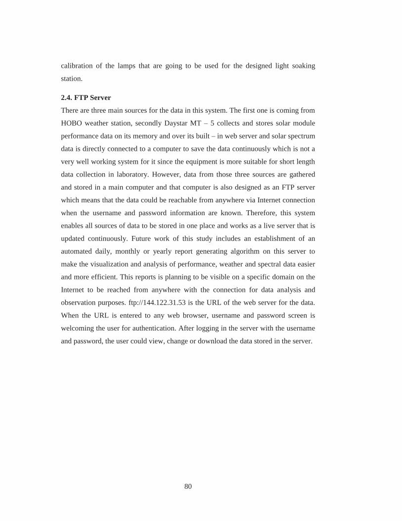
80
calibration of the lamps that are going to be used for the designed light soaking
station.
2.4. FTP Server
There are three main sources for the data in this system. The first one is coming from
HOBO weather station, secondly Daystar MT – 5 collects and stores solar module
performance data on its memory and over its built – in web server and solar spectrum
data is directly connected to a computer to save the data continuously which is not a
very well working system for it since the equipment is more suitable for short length
data collection in laboratory. However, data from those three sources are gathered
and stored in a main computer and that computer is also designed as an FTP server
which means that the data could be reachable from anywhere via Internet connection
when the username and password information are known. Therefore, this system
enables all sources of data to be stored in one place and works as a live server that is
updated continuously. Future work of this study includes an establishment of an
automated daily, monthly or yearly report generating algorithm on this server to
make the visualization and analysis of performance, weather and spectral data easier
and more efficient. This reports is planning to be visible on a specific domain on the
Internet to be reached from anywhere with the connection for data analysis and
observation purposes. ftp://144.122.31.53 is the URL of the web server for the data.
When the URL is entered to any web browser, username and password screen is
welcoming the user for authentication. After logging in the server with the username
and password, the user could view, change or download the data stored in the server.

81
Figure 2-31 Entrance Screen for FTP Server
All data tagged according to the date could be found under the folders of the server.
Figure 2-32 Datascreen in the FTP Server

82
Figure 2-33 HOBO Folder and Files
2.5. Solar Module List and Justifications
There are 9 solar modules that are installed in our test station. All of them are labeled
and connected to the Daystar MT – 5 I – V curve tracer for the daily performance
and I – V curve measurements.
Figure 2-34 All panels in the station
1
2
3
4
5
6
7 8 9

83
Figure 2-35 Daystar MT – 5 load (below) and control unit (top)
Nomenclatures of the tables are listed below;
PMAX: Maximum Power
IMP: Current at Maxiumum Power Point
VMP: Voltage at Maximum Power Point
ISC: Short Circuit Current
VOC: Open Circuit Voltage
2.5.1. Solar Modules List
Solar modules list is shown in Table 2-1.

84
Tab
le 2
-1 L
ist o
f Ins
talle
d So
lar M
odul
es
#
of
Cel
ls
60
72
60
36
180
72
60
T C
oeff
. Is
c
(%/°
K)
0.03
0.03
0.04
2
0.02
5
0.07
0.03
0.03
T C
oeff
. V
oc
(%/°
K)
-0.3
6
-0.3
6
-0.3
23
-0.3
6
-0.3
-0.3
6
-0.2
5
T C
oeff
. Pm
ax
(%/°
K)
-0.5
5
-0.5
5
-0.4
64
-0.4
5
-0.2
4
-0.5
5
-0.3
VO
C
(V)
36.6
43.7
37.1
21.7
59.8
43.7
42.3
I SC
(A)
8.7
5.06
8.45
8.18
3.45
5.06
7.22
VM
P
(V)
30.2
35
30.3
17.8
45.4
35
34.3
I MP
(A
)
7.96
4.58
7.94
7.3
2.82
4.58
6.71
P MA
X
(W)
240
160
240
130
128
160
230
Tec
h.
Poly
crys
tal
Silic
on
Mon
ocry
stal
Silic
on
Mon
ocry
stal
Silic
on
Poly
crys
tal
Silic
on
A.T
hin
Film
Si
licon
Mon
ocry
stal
Si
licon
M
onoc
ryst
al
HIT
Bra
nd
Chi
ner N
ew E
nerg
y C
R 2
40
Chi
ner N
ew E
nerg
y C
R 1
60
Isof
otón
ISF
– 24
0
Sola
rA
S520
P36
(SM
520S
)
Shar
p N
A
– F1
28G
5
Chi
ner N
ew E
nerg
y C
R 1
60
Sany
o H
IP
– 23
0 H
DE1

85
CHAPTER 3
3. LIGHT SOAKING STATION DESIGN
3.1. Overview of the Design
In addition to building an outdoor panel testing facility, a secondary purpose of this
project is to put together a light soaking station in which panels can be tested and
characterized under controlled conditions. By comparing the performance and
degradation behaviour of the panels on the outdoor test station vs. the light soaking
station, one can put together protocols for accelerated testing of panels – thereby
reducing the time taken to characterize the stabilized or long term efficiency of
produced panels.
The design of our light soaking station needs to satisfy cost vs. performance
constraints. On the one hand, we need to deliver a solar spectrum and intensity that is
as close to solar radiation as possible on a relatively large area (at least 1m by 1m)
while keeping costs to a minimum level. Our design is based upon the patent named
“Light Soaking System and Test Method for Solar Cells” [114]. Numbers on the
figures are the component codes in the related patent.
3.2. Choice of the Light Source
The first decision that needs to be made in the design is to choose the type of light
source. Xe arc lamps are the most suitable choice as far as the solar spectrum is
concerned. As shown in Figure 3-3, the spectral distribution from these types of
lamps show a good overlap to the solar spectra as measured on the surface of the
earth. The match can be made even better when specific filters are used to filter out
some of the unmatched peaks. However this is a very expensive solution for our

86
application. A 1000W Xe arc lamp can easily cost above $1000, let alone any
equipment to filter out the undesired peaks.
Figure 3-1 The patented light soaking design [114]
Figure 3-2 Side and Top view of LID Station
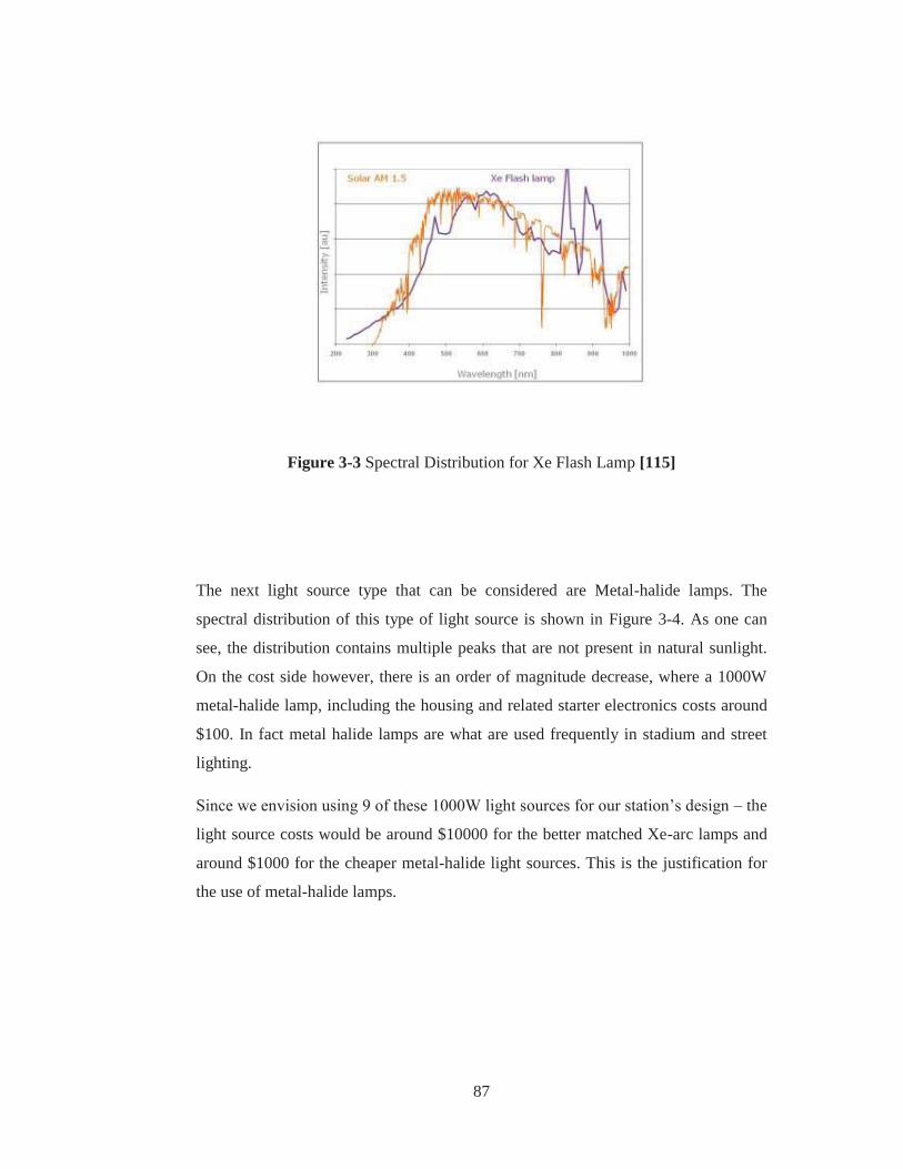
87
Figure 3-3 Spectral Distribution for Xe Flash Lamp [115]
The next light source type that can be considered are Metal-halide lamps. The
spectral distribution of this type of light source is shown in Figure 3-4. As one can
see, the distribution contains multiple peaks that are not present in natural sunlight.
On the cost side however, there is an order of magnitude decrease, where a 1000W
metal-halide lamp, including the housing and related starter electronics costs around
$100. In fact metal halide lamps are what are used frequently in stadium and street
lighting.
Since we envision using 9 of these 1000W light sources for our station’s design – the
light source costs would be around $10000 for the better matched Xe-arc lamps and
around $1000 for the cheaper metal-halide light sources. This is the justification for
the use of metal-halide lamps.

88
Figure 3-4 Spectral Distribution of a Metal Halide Lamp [116]
3.3. Choice of Instrumentation
In addition to aging the panels under the light, the light soaking station also needs to
have the capability to monitor panel performance as well as ambient conditions. This
functionality can be delivered by a piece of equipment that is similar to the DayStar
Multi-tracer which was utilized in the outdoor test station. However with a cost of
around $50000, this highly capable option is again out of reach due to cost
constraints.
Instead, we propose to deliver the same capability using modules supplied by
National Instruments combined by a PC and LabView software. The main module in
such a set-up is a 4 quadrant power supply that will enable light and dark IV
measurements, namely a NI PXI-4130. This power supply can deliver -20 to +20V
with a maximum current of 2A. This range can be extended by using multiple NI
PXI-4130 modules if needed. This power supply is coupled to a NI PXI-2527, a high
voltage multiplexer module that is capable of switching a single input to 16 outputs.

89
This combination allows for NI PXI-4130 to be used to capture IV curves for 16
panels – the measurements cannot be simultaneous but rather successive. The
environmental conditions can be monitored through a NI PXI-6220, which is a high
speed analog input module. A total of 16 channels can be connected to this analog
input module which can include panel or ambient temperatures through
thermocouples or other suitable temperature sensors as well as light intensity through
standard cells or pyranometers. These three modules are enclosed in a NI PXIe-1073
chassis and connected to the PC through a PCI-express interface. This set-up is
pictured in Figure 3-5.
Figure 3-5 Picture of the Chassis with the cards installed
The PC used is an HP brand machine with an Intel I3 family processor with 8GB of
RAM and a 500GB hard-disk. Combined with an academic license for LabVIEW 10
software, the total cost of the monitoring system is around $12000. The LabVIEW
code has been put together in house.
3.4. Lamp Configuration and Station Housing Design
Once the aforementioned choices are made, the next problem to be addressed is how
to configure the multiple light sources and how to design the enclosure and auxiliary
equipment to deliver as uniform intensity as possible with controlled ambient
conditions. The most significant issue to address besides light intensity distribution is

90
the temperature of the panels that are being aged. The multiple 1000W sources will
be delivering a significant thermal energy to the station and if not removed, the panel
temperatures will increase beyond limits that are appropriate for characterization
purposes. The cooling in the system will be achieved by using 10 fans that are 20cm
in diameter. These will be arranged in a very similar fashion to what is used to cool
computer cases – that is one set of fans will be drawing in air from the outside and a
second set will be exhausting from the opposite side. This will provide for a fresh air
circulation within the enclosure and by positioning the panels in this air flow,
convective cooling will cause the panel temperatures to be maintained at appropriate
levels, despite radiative heating from the light sources. If this approach fails to
deliver enough cooling, the next option is to equip the panel holding plate with an
active cooling mechanism that should also deliver a conductive cooling mechanism
to the panels. This will require an additional temperature controlled bath and a
recirculating pump. However this would also provide the capability to actively adjust
panel temperatures during testing.
The light source configuration was decided and characterized in two steps. We begin
by characterizing the distribution from a single light source. Then we use this set of
measurements as the basis of a model that evaluates the additive light from multiple
sources. Based on the results of this model, we finalize our housing design –
incorporating a mechanism for adjusting the light source to panel distance. This
adjustable distance will be fine-tuned upon construction of the equipment as the
model predictions may not be perfect. Furthermore being able to adjust the
separation will let us run aging tests at intensity conditions that are higher or lower
than the standard 1000W/m2 as well as allowing us to bring the panels closer slightly
as the light bulbs age over time. These activities will be summarized in the upcoming
sections.

91
3.4.1. Single Light Source Characterization
We chose to use 1000W light sources from the GE company – along with the bulb
housing and required starter components. These are pictured in Figure 3-6.
As one can see – this is the type of light source that is used to light sport fields and
parking lots. The light source itself is actually a very small – in the shape of a
cylinder that is approximately 10mm long with a diameter of around 3-5mm. The
reflector is in the shape of a rectangle with 365x393mm. The reflector edges are at an
angle of 30° on the long edge and 23° on the short edge. Due to this asymmetry, one
needs to make a choice on how to orient the multiple lamps to deliver an intensity
distribution that is as uniform as possible.
Figure 3-6 Picture of the single light source and the starter
We chose to characterize the distributions from the light source at distances of 50cm,
100cm, 150cm and 200cm. Due to the angles of the edges, the light intensity drops
very sharply to zero when one moves outside of the zone of direct exposure to the
source. Therefore the spacing of the grid needed to be adjusted according to the
distance to the light source in order to be able to characterize the lamp as accurately
as possible for the subsequent modeling activity. This is reflected in the grid
definition appearing in

92
Figure 3-7 below. Light intensity are measured by a KIMO SL 100 Solarimeter –
which utilizes a standard polycrystalline reference cell for capturing the light
intensity [117]
Figure 3-7 Single light source intensity distributions - intensity measurements are in
terms of w/m2 and grid data are in terms of cm.
x/y -43 -30 -20 -10 0 10 20 30 43
35 0 0 0 0 0 0 0 0 0
30 0 83 106 138 150 118 92 66 0
20 0 121 161 203 217 179 133 96 0
10 0 278 394 477 513 455 369 248 0
0 0 461 654 785 834 762 624 427 0
-10 0 344 488 609 656 585 459 315 0
-20 0 165 228 279 288 269 209 140 0
-30 0 80 113 141 151 129 99 71 0
-35 0 0 0 0 0 0 0 0 0
50cm - delta - 10 cmx/y -73 -51 -34 -17 0 17 34 51 73
56 0 0 0 0 0 0 0 0 0
51 0 25 31 36 37 35 30 24 0
34 0 41 54 62 67 63 54 43 0
17 0 88 121 150 161 146 127 95 0
0 0 127 180 239 249 223 183 131 0
-17 0 90 116 137 145 130 106 78 0
-34 0 47 57 64 64 59 50 38 0
-51 0 25 32 38 40 37 32 25 0
-56 0 0 0 0 0 0 0 0 0
100cm - delta - 17cm
x/y -102 -72 -48 -24 0 24 48 72 102
77 0 0 0 0 0 0 0 0 0
72 0 13 16 17 18 10 16 13 0
48 0 21 26 32 34 33 29 23 0
24 0 43 56 74 77 73 61 49 0
0 0 56 78 102 108 96 76 57 0
-24 0 36 48 57 58 53 44 34 0
-48 0 22 25 29 28 26 22 17 0
-72 0 12 16 19 19 18 15 12 0
-77 0 0 0 0 0 0 0 0 0
150cm - delta - 24cmx/y -131 -93 -62 -31 0 31 62 93 131
97 0 0 0 0 0 0 0 0 0
93 0 7 9 10 10 10 10 8 0
62 0 11 15 18 20 20 17 14 0
31 0 23 31 42 45 43 36 29 0
0 0 29 41 54 58 53 43 33 0
-31 0 19 24 31 32 30 25 19 0
-62 0 12 14 16 16 15 12 10 0
-93 0 7 9 10 10 10 9 7 0
-97 0 0 0 0 0 0 0 0 0
200cm - delta - 31cm

93
Figure 3-8 Various orientations of the 9 lamps considered
3.4.2. Multiple Light Source Modeling
The single source data are then supplied to a MATLAB code that can arrange
multiple light sources in various orientations then predict the combined distribution
based on the assumption that multiple light sources are purely additive, with no
interactions or reflections from external walls. This simple approach is deemed
appropriate for making preliminary design decisions. The code appears in and very
simple in logic. It takes in the single light source distribution and the desired
combination of 9 light sources. Then appropriately shifts and rotates the single light
source intensity distribution according to orientation and location, finally adding up
all the correctly shifted and rotated single source distributions. In our evaluation, we
considered the orientations appearing in

94
Figure 3-8 below where the arrow represents the location of the light bulb. These five
combinations cover all possibilities of systematically placing the lamps to capture the
effects of the asymmetry of the individual sources.
An additional variable that needs consideration is the spacing between the light bulbs.
If all light sources are placed right next to each other with no space in between, we
can get a spacing of 40cm between the centers of each bulb. However one may be
able to extend this further and evaluate its impact on uniformity and intensity.
Therefore this spacing was simulated at two additional levels to the 40cm minimum,
namely at 45cm and 50cm.
The typical results for the combinations appearing in Figure 3.8 are shown in Figure
3.9 below in terms of contour plots where the light intensity is highest for red and
successively drops to orange, yellow and blue at the lowest levels. As one can easily
appreciate, the configurations different than the two alternating options provide
regions of very low and very high intensity right next to each other due to the
asymmetric nature of the rectangular lamp housings with the different edge slopes.
Therefore the choice of orientation should definitely be one of the alternating options.
This summary shows that the alternating options are no different than each other.
Both deliver at least 1.5X better uniformity than their counterparts for the other
orientation options. The rotated options deliver slightly higher average power but this
does not justify the uniformity degradation. Furthermore the lamp separation delivers
an optimum for the 45cm option. As the lamps are further separated or brought closer
together, the uniformity of ~11% is degraded. This optimal comes at a cost of
reduced overall intensity as compared to the lamps that are closer but the additional
uniformity justifies this loss. Furthermore the minimum separation of 40cm may
cause difficulties when trying to build the support structure for the lamp housings. So
this additional 5cm would actually make the design and construction easier. Based on
these findings, our final design is configuration is fixed as the alternating 1
configuration with 45cm separation between the lamp centers.

95
Figure 3-9 Distribution at 45 cm lamp separation and 50 cm between the lamps and
the panels
At 50 cm light source to panel separation, we project to get an overall intensity of
777 W/m2 averaged over an area of 1m by 1m. This will be slightly closer to the
1000W/m2 standard in a 80x80cm square in the middle – however still not quite
there. Thus the table needs to be located closer than 50cm to the lamps. When the
data for 100 cm, 150 cm and 200 cm are evaluated in a similar fashion and one uses
the inverse square law to predict at lower values than 50 cm – one can predict a
separation of 42 cm for an intensity of 1000W/m2 for the given configuration – based
on the correlation of

96
Figure 3-10. Therefore the decision is made to place the bottom of the 20 cm
diameter fans at 50 cm away from the light sources so that the table can be adjusted
between 30 and 50 cm while still being in the direct path of the air circulation.
3.5. Finalized Design and Equipment
Based upon the decisions made using the data generated by the model of the previous
sections, the light soaking station was built in the METU Chemical Engineering
Department’s machine shop. Several angles are pictures in
Figure 3-10 Average intensity as a function of separation - inverse square behavior
y = 2E+06x + 20,801 R² = 0,9999
0
100
200
300
400
500
600
700
800
900
0 0,0001 0,0002 0,0003 0,0004 0,0005
Inte
nsity
(W/m
2)
1/d2 (1/cm2)

97
Table 3-1 Summary of the simulation results
# Lamp
Orientation
Table
Height
(cm)
Lamp
Separation
(cm)
Mean
(W/m2) Sigma
%
Sigma
1 All Same 50 40 922 204 22.1
2 All Same 50 45 777 209 26.9
3 All Same 50 50 652 215 33.0
4 Altern 1 50 40 922 129 14.0
5 Altern 1 50 45 777 87 11.2
6 Altern 1 50 50 625 112 17.9
7 Altern 2 50 40 922 129 14.0
8 Altern 2 50 45 777 87 11.2
9 Altern 2 50 50 625 113 18.1
10 Edges
Rotated 50 40 952 221 23.2
11 Edges
Rotated 50 45 797 193 24.2
12 Edges
Rotated 50 50 627 183 29.2
13 Middle
Rotated 50 40 892 238 26.7
14 Middle
Rotated 50 45 757 186 24.6
15 Middle
Rotated 50 50 623 181 29.1

98
Figure 3-11 The Final Construction of the Light Soaking Station
Figure 3-11 below. One can see here all the features mentioned in the previous
sections. 5 fans on one side take in the air and the 5 fans on the opposite side exhaust.
Each fan has a capacity of circulating 300m3 or air per hour. There are two handles
on either side of the table for a total of four support points. These rods can be
manually adjusted to move the table between 30cm and 62cm away from the light
source. They can be made longer to bring the table even closer but then the table is
beyond the region where air is circulated and this could cause cooling problems. The
starters are placed on two shelves on two sides of the enclosure. The table
dimensions are 135 cm by 135 cm. The 9 light sources used are all independently
controlled, meaning that any combination can be turned on or off as desired.

99
CHAPTER 4
4. RESULTS AND ANALYSIS
4.1. PV Performance Monitoring Station Analysis
4.1.1. Data Integrity Issues
There were several issues which had to be dealt with in order to improve the quality
and the continuity of the data generated by the performance monitoring station.
These are going to be outlined in more detail under two separate headings below –
one related to unforeseen fault issues and the other a more fundamental design issue
while setting-up the measurements.
4.1.1.1. Missing Data and Corrupt Sensor Problems
As will be apparent in the upcoming trend analyses, there will be periods of no
measurements. These are mostly due to specific sensor problems related to the
weather monitoring station. In particular there were problems with the pyranometer
used to measure solar irradiation – which was later resolved by providing adequate
electrical grounding to the module to discharge static electricity build-up, particularly
during windy conditions.
There was also another fault by the Daystar equipment in which the continuous
writing of the IV curves to the system’s hard drive – resulting in the loss of PV
performance data for a certain time period.
All of these shortcomings were addressed during this study and the system is
currently reliably collecting and archiving data.

100
4.1.1.2. Design Upgrade for Spectrophotometer (Shutter Arrangement)
Spectrophotometer was an important part of the outdoor test station since it was
going to provide spectral distribution of the sunlight in a continuous manner,
therefore makes it possible to compare and correlate the power data and I – V curve
measurements of the panels with different technologies and there could be a link
between the degradation modes and mechanism with the spectral distribution of the
sunlight, for instance different technologies could absorb different regions of the
spectrum causing different degradations in the molecular structure. However, the
nature of the equipment and the software are not very suitable for outdoor and
continuous data acquisition and the other alternatives that are designed for this
purposes mentioned above are very disadvantageous financially. The main problem
with the measurements is the need for taking periodical dark measurements for
calibrating the device. This does not seem practical and possible when the
spectrophotometer is operating in an outdoor environment with 24 hours of operation
since it is mainly designed for instant data capturing in a laboratory environment for
the experiments not lasting more than a day. Taking these periodic dark
measurements will not be feasible when the nature of a remote outdoor station is
concerned; therefore a shutter design is made to make this possible. A shutter with a
simple motor is designed to close the upper side of the sensor to prevent contact with
the sunlight in a desired interval or manually. Below, one can see the design of the
shutter with its components.
4.1.2. Trend Analysis on Historical Climatic Data
We have solar irradiation (and meteorological data) from the installed HOBO
Weather Station since April 2012 and reference meteorological data obtained from
Turkey Meteorological Data Archive and Management System (TÜMAS) between
the years of 2010 and 2013. There are a few periods where data is missing in HOBO
Weather Station. These are mainly due to the radiation sensor failure periods as
mentioned.

101
Figure 4-1 Shutter Design
Figure 4-2 and Figure 4-3 shows the distribution of the temperature and solar
irradiation data throughout the years of 2010 – 2013 in Ankara region respectively,
based upon the meteorological monitoring station located in Ankara. Specific
location is 39.97 North latitude and 32.86 East longitude. In comparison to the
METU weather monitoring station located at 39.89 North latitude and 32.78 East
longitude. The latitude of the two locations is 891 m and 914m respectively. The
distance between the two stations is approximately 17 km.
Therefore, this proximity of the reference meteorological station gives us a change to
calibrate and confirm identical measurements taken at our stations.
The impact of seasonal variations could be clearly seen when the official data is
investigated. The variation with respect to the seasons is quite predictable over the
course of 4 years that we have the data for.
There are two shortcomings related to meteorological data usage from this official
source. One is that this data is available only on an hourly basis whereas we capture
performance data from our panels on a minutely basis. Furthermore, although the
proximity of the two locations allows us to compare the average measurements over
a long period of time – individual measurements are still likely to be different due to
location specific, instantaneous atmospheric conditions such as could cover.

102
Figure 4-2 Reference Temperature Data throughout 2010 – 2013
Therefore we need to establish the validity of the for HOBO data, by direct
comparison to their counterparts from the TÜMAS database, which is the system that
collects and stores meteorological data from the reference stations. Correction factors
are calculated for HOBO data where appropriate.
The data comparison is simply plotting the data that belong to the same period in
time against each other to see if there is a strong correlation. In order to do that, the
data from HOBO and reference are taken and formatted to fit on to each other since
there are gaps in the timeline of the data collection because of the errors in the
HOBO system. In addition to that, the data taken from TÜMAS has hourly values of
the parameters while HOBO Weather Station measures and records data with the
intervals of ten minutes. Therefore, summary table and data merging tools of JMP

103
software is used to merge the data belonging to the same year, month, day, hour and
minutes. Lastly, time correction is made since TÜMAS values are in terms of
Greenwich Mean Time (GMT) while HOBO records measurements according to the
local time – so daylight savings time need to be considered. After this fitting
procedure, all parameters are readily compared with the reference values.
Figure 4-3 Reference Solar Irradiation Data throughout 2010 – 2013
The temperature comparison is shown in Figure 4-4. After the comparison of the data,
the following equation is found with R2 value of 0.98.
(4. 1)
Temperature value is in °C. The small intercept and the value of the slope close to
unity indicate that the HOBO measurements are within 5% of the reference
meteorological data – which is a reasonable fit.

104
Figure 4-4 Temperature Data Comparison
Figure 4-5 Pressure Data Comparison

105
The pressure correlation is demonstrated in Figure 4-5. This comparison indicates a
correlation coefficient, R2 of 0.99.
(4. 2)
Pressure value is in mbar. The pressure data from our weather monitoring station is
almost in complete agreement with the reference data.
Figure 4-6 Relative Humidity Data Comparison
As shown in Figure 4-6, the correlation of RH is much worse in comparison with the
pressure and temperature measurements outlined above. The value of R2 is 0.94.

106
(4. 3)
Relative humidity value is in (%). There is quite a significant off-set between the two
sources – but the trend is identical. So impact of RH on panel performance can be
evaluated, even though the absolute value of the variable may not necessarily very
accurate. There should not be this much discrepancy in RH values simply due to the
location difference between where the reference and our measurements are made.
Figure 4-7 Wind Speed Data Comparison
Wind speed and direction data do not show strong correlations at all – shown in
Figure 4-7 and Figure 4-8. This could be due to two weather stations being in
different locations which could have different wind amounts when the speed is
concerned – wind being a much more local variable that can be impacted by

107
geological features and man-made structures. In addition to that the range of
measurements, in particular of wind speed, is very narrow. We are most likely
sampling a lot of points at the lower end of our instrument’s range. As we sample
higher wind speeds, the trend may become more apparent.
Figure 4-8 Wind Direction Data Comparison
The aforementioned data are of secondary importance when solar panel performance
is considered. Solar panel power production is a very strong function of irradiation
and therefore this is perhaps the most important parameter that we need to calibrate.
The plot of the HOBO irradiance measurements vs. the references are shown in
Figure 4-9.

108
Figure 4-9 Solar Irradiance Data Comparison
When the solar irradiance data is investigated, it could be seen that two different
regions exist. The above region shows higher values for HOBO measurements in
terms of the reference irradiance while the below region which contain more data
seem to show a more even correlation between HOBO and reference values.
Furthermore it is seen that the group of data points belonging to the above region all
come from a specific time period towards the end of the summer of 2013, ending
with a complete sensor failure which resulted in replacement and repairs. Therefore,
it is decided to take these two regions separately to find the related correction factors
for HOBO measurements.
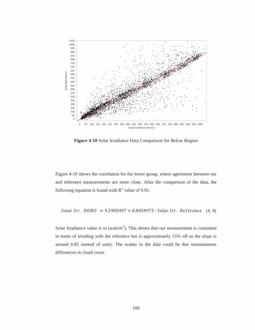
109
Figure 4-10 Solar Irradiance Data Comparison for Below Region
Figure 4-10 shows the correlation for the lower group, where agreement between our
and reference measurements are more close. After the comparison of the data, the
following equation is found with R2 value of 0.91. (4. 4)
Solar Irradiance value is in (watt/m2). This shows that our measurement is consistent
in terms of trending with the reference but is approximately 15% off as the slope is
around 0.85 instead of unity. The scatter in the data could be due instantaneous
differences in cloud cover.

110
Figure 4-11 Solar Irradiance Data Comparison for Above Region
We then look at the upper region in Figure 4-9 separately in Figure 4-11. After the
comparison of the data, the following equation is found with R2 value of 0.95.
(4. 5) Solar Irradiance value is in (watt/m2). Again there is a consistent trend but now more
than a 25% offset with respect to the reference is seen, in comparison to the 15%
offset in the opposite direction for the remaining dataset.
Table 4-1 below summarizes the intercept and slope values of the parameters in the
weather station for a linear fit with the reference data. These values are further used
to calculate the corrected values for HOBO Weather Station and used in the
performance characterization parameters of the solar modules. The significant values
are taken up to the last digit since they are going to be used in the correction formula
in this form, without rounding.

111
Table 4-1 Summary for Correction Values of Meteorological Parameters
Parameter Intercept Slope
Temperature 1.3756009 0.9546787
Pressure -4.381457 0.9994373
Relative Humidity 7.3141599 0.8306818
Solar Irradiance (Above Region) 5.2701976 1.2895323
Solar Irradiance (Below Region) 4.5905497 0.8454973
After the correction of the solar irradiance data – using different calibration factors
based on the slopes and intercepts summarized in Table 4-1, the correlation between
the reference irradiance and our measurements is very strong. The scatter is still there
as expected since we are calibrating based on the correlation of the data on an overall
basis.
Figure 4-12 Corrected HOBO Irradiance vs. Reference

112
(4. 6)
4.1.3. Correction for Module Tilt
One of the primary issues with the present set-up to capture solar irradiance data is
that the pyranometer that is used to capture the irradiation data and the solar panels
are at different levels of inclination with respect to the horizon. The pyranometer is
horizontal and equipped with a 180° cosine collector that captures the total incident
irradiation within its entire field of view. The panels, on the other hand, face directly
south and are inclined at an angle of 28.6° with respect to the horizontal. In fact all
panels in the northern hemisphere are directed towards the equator (or directly south)
and installed at ever increasing angles as one moves away from the equator. This is
to capture as much sun possible throughout the year. Thus a panel inclined at the
correct angle will receive, on the average, more irradiation than a horizontal panel.
One way to account for this discrepancy is to install the pyranometer at the same
level of inclination as the solar panels and it would be subjected to exactly the same
conditions as the panels. This however would invalidate any efforts to calibrate the
installed pyranometer against the reference data collected by the meteorology
department, who have pyranometers installed horizontally only. So even if one were
to install two pyranometers, one horizontal and the other inclined with the panels,
one would still have to be able to estimate the correlation between the two. The
estimation of this correlation depends on the specific position on the globe (which is
fixed by the coordinates of the station in terms of latitude and longitude) as well as
the precise position of the sun, which is a function of time of the day and the year.
4.1.3.1. Determination of the Tilt Correction
4.1.3.1.1. Horizontal to Tilted Irradiance – Geometrical Input
The equation that relates the irradiation, Es, on a surface tilted by s degrees from the
horizontal is given by
(4. 7)

113
Where Ebn is the direct normal irradiance, Ed is the diffuse horizontal irradiance; E is
the global horizontal irradiance.[118] The other factors appearing in this equation are
θ representing the angle of incidence of the sun rays on the tilted plane, Rd denoting
the diffuse transposition factor, ρ for the foregrounds’ albedo and finally Rr as the
transposition factor for ground reflection. The irradiance factors that appear on the
right hand side are also interrelated with the expression
(4. 8)
where Z denotes the zenith angle of the sun.
Using this second relationship, one may be able to use two out of the three irradiance
terms and calculate Es. However in our case, as is the case in many situations, Only E
is available (this is what is measured by the horizontal pyranometer) and Es must be
estimated based only on this component.
Further simplifications to this set of equations (based on ignoring the ground
reflections and the dependence of the diffuse irradiation to the sun’s position) results
in a purely geometrical relationship between the measured horizontal irradiance and
the inclined irradiance as
(4. 9)
Where the newly introduced variable, α, represents the solar elevation angle and is
given at any time by the relationship
(4. 10)
where ϕ is the latitude and δ is the declination angle of the sun.

114
4.1.3.1.2. Solar Position Estimation
Then the problem is reduced to determination sun with respect to the METU PV
performance monitoring station so that the time dependent declination angle and
elevation angle can be calculated.
There are several methods available in the literature to make these estimations. We
preferred the usage of the method utilized by the NOAA (National Oceanic and
Atmospheric Administration).[119] Their website provides downloadable and
editable spreadsheets whose prediction formulae can be directly integrated into our
MATLAB code. The details of the calculations can be found on their web-site which
indicates a very good level of accuracy between the years of 1800-2100. Like most
other solar vector estimation algorithms, the calculations depend on the
determination of the Julian century – which estimates the approximate position of the
earth on its solar orbit based on the current date and time. The celestial coordinates,
namely the declination and right ascension, estimated based on this position of earth
are then converted to the coordinate system that is centered on the position of the
globe where the observation station is located – as defined by the longitude and
latitude. Once this conversion is complete, the elevation and zenith of the sun is
calculated – which can then be used in (3) and (4) to convert the measured horizontal
irradiance to the inclined irradiance as seen by the modules.
4.1.3.2. Yearly Trends of Solar Position
The METU solar station is positioned at 39.39° North latitude and 32.72° East
longitude – based on the coordinates provided by Google Maps.[120] The local time
at any given point must be converted to the Coordinated Universal Time (UTC).
When daylight savings time is not in effect, local time in Turkey is UTC+2hrs. The
daylight savings time adds another hour, bringing Turkey to UTC+3hrs. The
beginning and end dates of the daylight savings time in Turkey over the past few
years can be found that the ministry of Energy’s website.[121] The general trend is
that daylight savings time begins in the last week of March and lasts until the last

115
week of October. The implementation is made during the night that connects the last
Saturday of the week to the last Sunday.
The location and daylight savings time correction have been coded into MATLAB
along with the NOAA algorithm that calculates the solar position. This code allows
for the determination of the correction factor to convert the measured horizontal
irradiation to the desired inclined irradiation for any given day and time.
This script was used to evaluate the solar position as a function of date and time for
the METU solar monitoring station. The data is summarized in terms of monthly
averages vs. time of the day in Figure 4-13. Sunset and sunrise is defined formally as
when the zenith angle crosses over the 90° value. As once can see, days get longer
and peak at around June and July, then fall back to minimum levels close to
December and January – in line with the summer and winter solstices falling on June
21st and December 21st respectively.
The presented modeling approach does have two significant shortcomings around
sunset and sunrise however. The NAOO algorithm demonstrates most errors in this
region as it does not incorporate the reflections that sunlight goes through in the
atmosphere. These effects are most pronounced during sunrise and sunset where the
angle of incidence of the sun rays is close to the horizon. Furthermore the
atmospheric effects that greatly influence the diffuse radiation are most significant
during these extreme times – and this effect is ignored in the geometrical only
approach that is taken to convert horizontal to inclined radiation.
In order to filter out these points, a more conservative definition of sunrise and sunset
is implemented – otherwise negative correction factors are possible. Based on the
analysis of the data, we define the presence of the sun in the sky for zenith angles
that are less than 80°, which systematically filters out the cases where the sun is very
close to the horizon. Beyond these points, we defined the correction factor as zero,
meaning that there is no sun in the sky. This actually does not impact our
calculations very significantly because these time periods correspond to very low

116
irradiation levels anyway and does not capture any significant power generation from
the modules.
Figure 4-13 Solar Zenith Angle
Based on this filter, the hourly average tilt correction factors are plotted in Figure
4-14, with respect to time of day. The larger dots represent the winter months, where
the correction factor is always above 1.0 – this compensates for the relatively lower
levels of solar irradiation during these months and tries to even out the total power
generation through the year. This however results in tilt correction factors that are
very close to 1.0 and actually lower than 1.0 during the hours right after sunrise and
right before sunset - during the summer months. So one may actually propose to
implement different inclination angles by season or month – with the extreme case of

117
this proposal being solar vector dependent inclination angles, which is the basis for
trackers. One would need to carry out a cost vs. benefit analysis here because any
dynamic change in inclination angle, even though on a seasonal basis, is going to
require some operational cost.
Figure 4-14 Tilt Correction Factors by Time of day, colored by month
4.1.4. Analysis of Solar Panel Performances
The HOBO data that is calibrated and confirmed with respect to the reference
measurements are then merged with the Daystar readings that capture the panel
performance. The HOBO irradiance data is also corrected for the module tilt as
outlined in Section 4.1.3. Panel performance is quantified based on regularly
captured IV traces from which the Daystar software automatically captures Pmax, Isc,

118
Voc and the FF. We have developed our own MATLAB code that further analyzes
the IV traces to capture Rs and Rsh values from the slopes near Voc and Isc points.
With this data set at hand, it will be possible to correlate all relevant performance
metrics to meteorological conditions. The number of valid data points per installed
panel and technology are outlined in Table 4.2.
For analysis purposes, the radiation levels are also grouped into specific irradiance
bins – to see later on in the analysis whether some correlations exist with respect to
the irradiance level. Again this grouping is made based upon the irradiance level that
is corrected for module tilt.
It is also customary to normalize power outputs with respect to nominal panel
production and the level of irradiance in order to be able to compare a large dataset
involving panels of different technologies. The specifics of the metrics introduced
below are explained in Section 1.3.7. First the final yield normalizes the power
output with respect to nominal panel output at STC by (1. 5)
Then the reference yield is defined as solar radiation divided by the reference solar
radiation at STC which is 1000 W/m2. (1. 6)
Finally the performance ratio normalizes YF with YR to indicate whether the panel is
producing as much power as it should under the given irradiance conditions. (1. 7) If all measurements are correct, the PR can take a maximum and optimal value of
unity.

119
Table 4-2 Summary of Data Points
Panel ID Technology Data Points Date Installed
Chiner (160W) – Clean
Monocrystal
Silicon 4261 8/2/2012
Chiner (160W) – Dirty
Monocrystal
Silicon 7660 4/7/2012
Chiner (240W)
Polycrystal
Silicon 1981 4/7/2012
Isophoton (240W)
Monocrystal
Silicon 7372 4/7/2012
Sanyo HIT (230W)
Monocrystal
Heterojunction
with Intrinsic
Thin Layer 1813 6/28/2013
Sharp (128W)
Amorphous
Thin Film
Silicon 8914 4/7/2012
SolarA (130W)
Polycrystal
Silicon 4444 7/23/2012
Table 4-3 Grouping Radiation Levels
Sun Level # of Points LOW HIGH
4 3095 750 -
3 5808 500 750
2 3961 250 500
1 11416 0 250

120
We first investigate what drives power generation from the modules. The Voc and Isc
plots vs Pmax clearly show that increased power generation is driven most
significantly by Isc. The Voc values quickly reach their nominal values and stay there
for entire region for all technologies. This is the expected behaviour for photovoltaic
panels, where the power generation is driven by the number of photons – where
larger numbers generate more electron hole pairs resulting in larger photocurrent.
The Voc is a fundamental material property that does not change with the level of
irradiance.
Figure 4-15 Maximum Power vs. Short Circuit Current for Installed Panels
In Figure 4-17, we look more closely at the FF. The fill factor shows a steady
decrease with increasing power output as the panel approaches its nominal capacity.
This can be due to either increases in Rs or decreases in Rsh. We then look at these
two parameters in further detail in Figure 4-18 and Figure 4-19.

121
Figure 4-16 Maximum Power vs. Open Circuit Voltage for Installed Panels
Figure 4-17 Maximum Power vs Fill Factor for Installed Panels

122
It is clearly seen that the series resistance is changing in the positive direction as
power production increases whereas the shunt resistance is changing in the undesired
direction. So we can conclude that the loss of fill factor is due to the falling value of
Rsh, which is an indication of the increase in the slope of the IV curve where it nears
the Isc point. This is inline with the previous observation of Pmax being driven by the
Isc. The Voc point is relatively fixed and power generation is driven by increasing Isc
and as indicated by the falling Rsh and subsequently the FF, the portion of the IV
curve between Imax and Isc is not shifting up parallel to the horizontal axis but also
changing its slope slightly as Isc increases. This loss mechanism shows different
levels of significance depending on the module technology.
Figure 4-18 Maximum Power vs Series Resistance for Installed Panels
Next we investigate the overall performance of the panels based on their
performance ratios. The box plot in Figure 4-20 is generated to make this comparison.
Note that there are still some points for PR greater than unity, which means that there
are still some inaccuracies in our solar irradiance data. However more than 95% of
the data points included are below unity in terms of performance ratio.

123
Figure 4-19 Maximum Power vs Shunt Resistance for Installed Panels
Figure 4-20 Performance Ratio Comparison

124
When one makes a statistical evaluation of the performance ration metric, it is seen
that the panels fall into two distinct categories. Table 4-4 shows the pair wise t-test
comparison of the mean of the PR with a 95% confidence level. The monocrystalline
based technologies are in the upper groups where as the polycrystalline and
amorphous thin film technologies fall into the second category. Among the upper
group, the heterojunction technology shows superior performance – and among the
lower group the amorphous technology shows the worst performance. However these
two conclusions are not statistically justified at the 95% level.
The PR metric is also very useful when considering the impact of secondary factors
such as temperature, pressure and RH on panel performance because it normalizes
the impact of solar irradiance – which by far has the most significant on Pmax.
Therefore we investigate these impacts based on the PR.
This analysis is visualized in Figure 4.21 through Figure 4.23. It is seen; in general
that increasing temperature and decreasing RH have a negative impact on panel
performance. This is most strongly demonstrated at higher irradiation levels – thus
the aforementioned plots are generated for irradiance conditions that are larger than
750W/m2. Below 500W/m2, and particularly below 250W/m2, the correlations
gradually lose significance and eventually disappear. The pressure has no impact on
performance.
The loss in performance is inline with the expectations based on the negative
temperature coefficient at Pmax. It is very difficult to make a quantitative analysis
based on individual panels and PV technologies due to the large amount of scatter in
the data. It seems from a qualitative perspective that there are no significant
differences between the panels. The range of quoted temperature coefficients are
between 0.24 and 0.55; so one would expect to see some difference. However we
would have to generate more data to observe these differences.

125
Table 4-4 Statistical Comparison of Panel Performance Ratios
Level Category Mean
SANYO 230W A 0.8624
Chiner 160W (Dirty) A 0.8587
Chiner 160W (Clean) A 0.8424
Isofoton 240W A 0.8284
Chiner 240W B 0.7810
SolarA B 0.7781
Sharp 128W B 0.7703
A fundamental measurement issue could also be in play here, where we are assuming
that the ambient temperature is a direct indication of the panel temperature – which is
a questionable assumption. The temperature measurements in the HOBO station are
taken through a shaded temperature measurement device whereas the panels are
exposed to radiation and their temperature could vary significantly from those
measured under the shade. This is probably what is causing the scatter in the data and
can be resolved by installing thermocouples to monitor actual panel temperatures.
The Daystar equipment already has this monitoring capability.
The impact of RH can be attributed to the diffuse radiation component, where when
there is more moisture in the air, the diffuse component of the radiation is potentially
higher than the dryer conditions where the sunlight is not going to have as many
water molecules on its path.

126
4.2. LID Station Measurements
4.2.1. Light Intensity Measurements
Once the construction is made, the next step was to characterize the light distribution
and fine tune the spacing to deliver 1000W/m2 average intensity. We first look at
how long it takes for the light intensity to stabilize. For this purpose we fix the table
at 47cm, place the reference cell at a fixed position and begin the record the intensity
at 1 minute intervals. We see a very rapid increase in the first 10 minutes that then
very slowly stabilizes in the next 20 minutes. Based on this transient data, it would
be fair to say the output of the lamps stabilize within 30 minutes. Any further
characterization or aging study needs to take this into account.
Figure 4-21 Performance Ratio vs Temperature for Installed Panels

127
Figure 4-22 Performance Ratio vs Relative Humidity for Installed Panels
Figure 4-23 Performance Ratio vs Pressure for Installed Panels

128
Figure 4-24 Light Intensity as a Function of Time at 47 cm Table to Lamp
Separation
We then marked a 120x120cm grid centered on the center of the table with 20cm
interval spacing. We then proceeded to characterize the intensity distribution for
table to lamp separation distances of 47cm, 52cm and 63cm. A typical contour plot is
given in Figure 4-25 below. Once can immediately notice here that the points beyond
the 100x100cm square result in very poor light intensity as these locations are only
lit by the single lamps near the edges – no overlap is available to increase intensity.
These are numerically summarized in Table 4.5 where the average and standard
deviation of the intensity distributions are broken down by the smaller and larger
squares. At 52cm, the uniformity over the 100x100cm square is predicted to be 17%
- which is slightly higher than the modelled value of 12%. This can be a direct result
of the 20cm spacing on the grid which we took our measurements. We can further
refine this grid spacing to capture the uniformity and distribution with a higher
degree of accuracy. The mean of 861 W/m2 is somewhat higher than the predicted
0
200
400
600
800
1000
1200
0 10 20 30 40 50
Inte
nsity
(W/m
2)
Time (min)

129
value of 777 W/m2 – which again could be a direct result of inadequate sampling
during the characterization. However when one considers the crude nature of the
modeling approach, the resulting mismatch is not too unrealistic. Also based on these
measurements and the inverse square law, one can predict a separation of 38cm to
deliver a 1000 W/m2 average intensity over the 100x100cm square in the middle of
the table.
This one is for 47 cm separation. Remaining two separations show similar
characteristics.
Figure 4-25 Typical Contour Plots
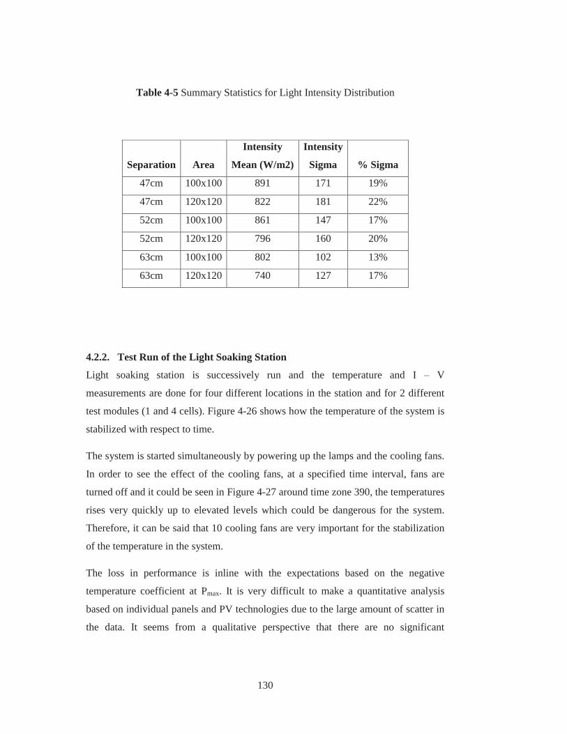
130
Table 4-5 Summary Statistics for Light Intensity Distribution
Separation Area
Intensity
Mean (W/m2)
Intensity
Sigma % Sigma
47cm 100x100 891 171 19%
47cm 120x120 822 181 22%
52cm 100x100 861 147 17%
52cm 120x120 796 160 20%
63cm 100x100 802 102 13%
63cm 120x120 740 127 17%
4.2.2. Test Run of the Light Soaking Station
Light soaking station is successively run and the temperature and I – V
measurements are done for four different locations in the station and for 2 different
test modules (1 and 4 cells). Figure 4-26 shows how the temperature of the system is
stabilized with respect to time.
The system is started simultaneously by powering up the lamps and the cooling fans.
In order to see the effect of the cooling fans, at a specified time interval, fans are
turned off and it could be seen in Figure 4-27 around time zone 390, the temperatures
rises very quickly up to elevated levels which could be dangerous for the system.
Therefore, it can be said that 10 cooling fans are very important for the stabilization
of the temperature in the system.
The loss in performance is inline with the expectations based on the negative
temperature coefficient at Pmax. It is very difficult to make a quantitative analysis
based on individual panels and PV technologies due to the large amount of scatter in
the data. It seems from a qualitative perspective that there are no significant

131
differences between the panels. The range of quoted temperature coefficients are
between 0.24 and 0.55; so one would expect to see some difference. However we
would have to generate more data to observe these differences.
Figure 4-26 Temperature vs Time Plot for Different Points in the LID Station
Figure 4-27 Time Period when the Cooling Fans are Turned off
10
30
50
70
90
0 100 200
Tem
pera
ture
(°C)
Time (min)
Lamp
Edge
Middle
Panel - 4 Cell
10
30
50
70
90
380 390 400 410 420
Tem
pera
ture
(°C)
Time (min)
Lamp
Edge
Middle
Panel - 4 Cell

132
Figure 4-28 shows the effect of lamps and the illumination amount on the test
module performances. In specified times during the trial experiment, some lamps are
randomly closed to see the effect on the temperature and performance of the test
modules. One can see by looking at Figure 4-28 that ISC decreases as the illumination
decreases while VOC does not change with respect to the illumination conditions.
Figure 4-28 I- V Curve under Different Illuminations for 1 Cell Module
The same behavior goes for the 4 cell module too, however if one looks closer to the
data, it could be observed that VOC is also changing for this module along with the
ISC.
The change in VOC seems to be related with the changing temperature because of the
decrease in the illumination in that area. Figure 4-30 shows the changing VOC values
and Figure 4-31 shows the correlation with the changing temperature.

133
Figure 4-29 I - V Curve under Different Illuminations for 4 Cell Module
Figure 4-30 Voc Change for 4 Cell Module

134
Figure 4-31 Voc Temperature Relationship for 4 Cell Module
4.3. Future Improvements
Further items that need to be fined tuned or upgraded on the light soaking station
include the modification of the characterization set-up to provide for adjustable loads
for the panels being tested while their IV curves are not being captured (which can be
achieved by the NI PXI-2527 switch for up to 8 panels simultaneously), upgrading of
the cooling set-up to provide for active conductive cooling on the table surface and
improvements to the user interface to further enhance user friendliness. Also
additional ambient condition monitors such as a reference cell can be included in the
set-up.

135
CHAPTER 5
5. SUMMARY AND CONCLUSIONS
In this study, the properties of commercial solar modules, characterization methods
and the degradation modes are discussed. An outdoor test station consisting of a
continuously working weather station and the module performance measuring I – V
tracer is installed and a light soaking station is designed and operated in order to
conduct accelerated tests for the sample modules. It is observed that continuous data
collection requires high amount of automated hardware and software in order to fully
avoid errors and data loss. It is also very important to backup the data stored in the
outdoor station. For this purpose, An FTP server is established to automatically get
the data from equipments and store them in a place that could be reached remotely
and safely. Statistical analysis made upon the merging of the performance and
meteorology data show that solar irradiation and temperature are primarily important
for the performance of the solar modules. Other variables like pressure, humidity are
of secondary concern. Solar irradiance collected by HOBO U30 Weather Station is
calibrated considering the inclination of the modules along with the solar vector and
latitude and longitude information. Performance metrics for the solar modules show
that monocrystalline panels show better performance in terms of PR than the
polycrystalline and thin film technologies respectively. For the light soaking station,
temperature control in the test chamber is very important to conduct accelerated tests
in a stabilized environment. The designed system requires a stabilized temperature
for the tests, however further modification is needed if the temperature is wanted to
be hold in a specific value for testing purposes. In addition to that, the light soaking
station designed in this study could characterize the sample modules with their
temperature and I – V curve measurements on a basic basis.

136

137
REFERENCES
[1] T. J. M. Oliver, “The market for solar photovoltaics,” Energy Policy, pp. 371-385, 1999.
[2] V.V.Tyagi, “Progress in solar PV technology: Research and achievement,” Renewable and Sustainable Energy Reviews, pp. 443-461, 2013.
[3] “European Photovoltaic Industry Association,” 2008. [Online]. Available: http://www.epia.org/about-us/about-photovoltaics/solar-photovoltaic-technology/.
[4] Paolo Frankl, Stefan Nowak, Marcel Gutschner, Stephan Gnos, Tobias Rinke, “Technology Roadmap Solar photovoltaic energy,” International Energy Agency, 2010.
[5] “Photovoltaic (PV) Cell,” 2011. [Online]. Available: https://sites.google.com/site/reeetech/home/photovoltaic .
[6] T. Saga, “Advances in crystalline silicon solar cell technology for industrial mass production,” NPG Asia Materials, pp. 96-102, 2010.
[7] Y. Chu, August 2011. [Online]. Available: http://www.geni.org/globalenergy/research/review-and-comparison-of-solar-technologies/Review-and-Comparison-of-Different-Solar-Technologies.pdf.
[8] M. W. Alan Goodrich*, “A wafer-based monocrystalline silicon photovoltaics road map: Utilizing known technology improvement opportunities for further reductions in manufacturing costs,” Solar Energy Materials & Solar Cells, pp. 110-135, 2013.
[9] G. Simbolotti, “Solar Photovoltaics Technology Brief,” IEA-ETSAP, 2013.
[10] R. H. Bube, Photovoltaic Materials, 1998.
[11] Martin A. Green, Keith Emery, Yoshihiro Hishikawa, Wilhelm Warta,Ewan D. Dunlop, “Solar cell efficiency tables (version 42),” Progress in Photovoltaics, pp. 827-837, 2013.
[12] “Energy Technology Perspectives,” 2008.

138
[13] R.W. Miles*, K.M. Hynes, I. Forbes, “Photovoltaic solar cells: An overview of state-of-the-art cell development and environmental issues,” Progress in Crystal Growth and Characterization of Materials, pp. 1-42, 2005.
[14] A. Goetzberger, W. Shockley, “Journal of Applied Physics,” p. 409, 1960.
[15] Adolf Goetzberger, Christopher Hebling, Hans-Werner Schock, “Photovoltaic materials, history, status and outlook,” Reports: A Review Journal, pp. 1-46, 2003.
[16] M. A. Green, “Crystalline and thin-film silicon solar cells: state of the art and future potential,” Solar Energy, pp. 181-192, 2003.
[17] Bhubaneswari Parida, S. Iniyan, Ranko Goic, “A review of solar photovoltaic technologies,” Renewable and Sustainable Energy Reviews, p. 1625–1636, 2011.
[18] T. Markvart, Solar Electricity, 1995.
[19] D. L. King and J. A. Hansen, “Proceedings of the 25th IEEE PV Specialists Conference,” in Dark current-voltage measurements on photovoltaic modules as a diagnostic or manufacturing tool, 1997.
[20] S. R. Rummel and T. J. McMahon, “13th NREL Photovoltaics Program Review,” in Effect of cell shunt resistance on module performance at reduced light levels, Lakewood, 1995.
[21] Edson L. Meyer and E. Ernest van Dyk, “IEEE TRANSACTIONS ON RELIABILITY,” in Assessing the Reliability and Degradation of Photovoltaic Module Performance Parameters, 2004.
[22] S. Durand, “Attaining Thirty-Year Photovoltaic System Lifetime,” Progress in Photovoltaics: Research and Applications, 1994.
[23] Wenger HJ, Schaefer J, Rosenthal A, Hammond B, Schlueter L., “Decline of the Carrisa Plains PV Power Plant: The Impact of Concentrating Sunlight on Flat Plates,” in 22nd IEEE Photovoltaic Specialists Conference, 1991 .
[24] F. J. Pern, “Ethylene-vinyl acetate (EVA) encapsulants for photovoltaic modules: Degradation and discoloration mechanisms and formulation modifications for improved photostability,” Die Angewandte Makromolekulare Chemie, pp. 195-216, 1997.
139
[25] J. Pern, “Module Encapsulation Materials, Processing and Testing,” Shanghai, 2008.
[26] D. C. Jordan and S. R. Kurtz, “Photovoltaic Degradation Rates-an Analytical Review,” Progress in Photovoltaics: Research and Applications, p. 12–29, January 2013.
[27] W. H. Holley, S. C. Agro, J. P. Galica, L. A. Thoma, R. S. Yorgensen, M. Ezrin, P. Klemchuk, and G. Lavigne, “Investigation into the causes of browning in EVA encapsulated flat plate PV modules,” in Conference Record of the 24th IEEE Photovoltaic Specialists Conference, Waikoloa, 1994.
[28] D. Berman, S. Biryukov, and D. Faiman, “EVA laminate browning after 5 years in a grid-connected, mirror-assisted, photovoltaic system in the Negev desert: effect on module efficiency,” Solar Energy Materials and Solar Cells, p. 421–432, April 1995.
[29] Lawrence Dunn, Michael Gostein and Bill Stueve, “Literature Review of the Effects of UV Exposure on PV Modules,” 2013.
[30] Kempe, M.D., Jorgensen, G.J., Terwilliger, G.J., McMahon, T.J.,Kennedy, C.E., Borek, T.T., “Acetic acid production and glass transition concerns with ethylene-vinyl acetate used in photovoltaic devices,” Solar Energy Materials & Solar Cells, p. 315–329, 2007.
[31] P. Klemchuk, M. Ezrin, G. Lavigne, W. Holley, J. Galica, and S. Agro, “Investigation of the degradation and stabilization of EVA-based encapsulant in field-aged solar energy modules,” Polymer Degradation and Stability, p. 347–365, March 1997.
[32] F. J. Pern and A. W. Czanderna, “EVA degradation mechanisms simulating those in PV modules,” pp. 445-452, 1992.
[33] M. Kempe, “ Ultraviolet test and evaluation methods for encapsulants of photovoltaic modules,” Solar Energy Materials & Solar Cells, p. 246–253, 2010.
[34] Abdérafi Charki, Rémi Laronde, David Bigaud, “Accelerated degradation testing of a photovoltaic module,” Journal of photonics for energy, 2013.
[35] Ethan Wang, Hsinjin Edwin Yang, Jerry Yena, Sunny Chia, Carl Wanga, “Failure Modes Evaluation of PV Module via Materials Degradation Approach,” Energy

140
Procedia, pp. 256-264, 2013.
[36] Claudio Ferrara and Daniel Philipp, “Why Do PV Modules Fail?,” Energy Procedia, pp. 379-387, 2012.
[37] N. Bosco, “Reliability Concerns Associated with PV Technologies,” 2010.
[38] M. Kemp, “Control of moisture ingress into photovoltaic,” in 31st IEEE Photovoltaic Specialists Conference and, Florida, 2005.
[39] Munoz, M.A., Alonso-Garcia, M.C., Nieves, V., Chenlo, F., “Early degradation of silicon PV modules and guaranty conditions,” Solar Energy, p. 2264–2274, 2011.
[40] Carlson, D.E., Romerol, R., Willing, F., Meakin, D., Gonzalez, L.,, “Corrosion effects in thin film photovoltaic modules,” Photovoltaics: Research and Applications, p. 377–386, 2003.
[41] Osterwald, C.R., Anderberg, A., Rummel, S., Ottoson, L., “Degradation Analysis of Weathered Crystalline-Silicon PV Modules,” in IEEE Photovoltaic Specialists Conference, New Orleans.
[42] Ababacar Ndiaye, Abde'rafi Charki, Abdessamad Kobi, Cheikh M.F. Kebe,, “Degradations of silicon photovoltaic modules: A literature review,” Solar Energy, p. 140–151, 2013.
[43] Oreski, G., Wallner, G.M., “Evaluation of the aging behavior of ethylene copolymer films for solar applications under accelerated weathering conditions,” Solar Energy, pp. 1040-1047, 2009.
[44] Kojima, T., Yanagisawa, T., “The evaluation of accelerated test for degradation a stacked a-Si solar cell and EVA films,” Solar Energy Materials & Solar Cells, pp. 119-123, 2004.
[45] Wohlgemuth, J.H., Kurtz, S., “Reliability Testing Beyond Qualification as a Key Component in Photovoltaic’s Progress Toward Grid Parity,” in IEEE International Reliability Physics Symposium, California, 2011.
[46] M. Kempe, “Modelling the moisture ingress into photovoltaic modules,” Solar Energy Materials & Solar Cells, p. 2720–2738, 2006.
[47] Kaplanis, S., Kaplani, E., “Energy performance and degradation over 20 years performance of BP c-Si PV modules,” Simulation Modeling Practice and Theory,

141
pp. 1201-1211, 2011.
[48] Lombardo T, Ionescu A, Lefe`vre RA, Chabas A, Ausset P, Cachier H, “Soiling of silica-soda-lime float glass in urban environment: measurements and modeling,” Atmospheric Environment, 2005.
[49] Skoczek, A., Sample, T., Dunlop, E.D., Ossenbrink, H.A., “Electrical performance results from physical stress testing of commercial PV modules to the IEC61215 test sequence,” Solar Energy Materials & Solar Cells, p. 1593–1604, 2008.
[50] Jansen, K.W., Delahoy, A.E., “A laboratory technique for the evaluation of electrochemical transparent conductive oxide delamination from glass substrates,” Thin Solid Films , p. 153–160, 2003.
[51] Paula Sanchez-Friera, Michel Piliougine, Javier Pelaez, Jesus Carretero and Mariano Sidrach de Cardona, “Analysis of degradation mechanisms of crystalline silicon PV modules after 12 years of operation in Southern Europe,” Progress in Photovoltaics: Research and Applications, pp. 658-666, 2011.
[52] H. J. Möller, “Semiconductors for Solar Cells: Artech House,” p. 41–46, 1993.
[53] E. L. Meyer and E. E. van Dyk, “Proceedings of the 17th European Photovoltaic Solar Energy Conference,” in Monitoring I - V and performance parameters of photovoltaic modules, 2001.
[54] Stephan, M., Thomas, K., Wolfgang, J., Hurbert, F., “Proceedings of the 19th EU PVSEC,” in Quality testing for PV modules according to standards and performance control for supporting manufacturing, Paris, 2004.
[55] Kempe MD, Jorgensen GJ, Terwilliger KM, McMahon TJ, Kennedy CE, Borek TT, “Proceedings of the 4th World Conference on Photovoltaic Energy Conversion,” in Ethylene-vinyl acetate potential problems for photovoltaic packaging, 2006.
[56] Quintana, M.A., King, D.L., McMahon, T.J., Osterwald, C.R., “Commonly observed degradation in field-aged photovoltaic modules,” in Proceedings 29th IEEE Photovoltaic Specialists Conference, 2002.
[57] Dallas, W., Polupan, O., Ostapenko, S., “Resonance ultrasonic vibrations for crack detection in photovoltaic silicon wafers,” Measurement Science and Technology, p. 852–858, 2007.

142
[58] Rueland, E., Herguth, A., Trummer, A., Wansleben, S., Fath, P., “Optical l-crack detection in combination with stability testing for inline inspection of wafers and cells,” in Proceedings of 20th EU PVSEC, Barcelona, 2005.
[59] Schütze, M., Junghanel, M., Friedrichs, O., Wichtendahl, R., Scherff, M., “Investigations Of Potential Induced Degradation Of Silicon Photovoltaic Modules,” in 26th European Photovoltaic Solar Energy Conference, Hamburg, 2011.
[60] P. Hacke, “37th IEEE PVSC,” in System Voltage Potential-Induced Degradation, 2011.
[61] Molenbroek, E., Waddington, D.W., Emery, K.A., “Hot spot susceptibility and testing of PV modules,” in Conference Record of the 22th IEEE, Las Vegas, 1991.
[62] Rauschenbach, H., Mauder, E.E., “Breakdown phenomena in reverse biased silicon solar cells,” in Proceeding 9th photovoltaic specialist’s conference, 1972.
[63] W. Hermann,W.Wiesner, W.Vaaen, “Proceedings of the 26th IEEE PV Specialists Conference,” in Hot spot investigations on PV modules-new concepts for test standard and consequences for module design with respect to bypass diodes, 1997.
[64] E. E. van Dyk, B. J. Scott, E. L. Meyer, and A. W. R. Leitch, “Temperature dependence of performance of crystalline silicon photovoltaic modules,” South African Journal of Science, p. 198–200, 2000.
[65] Changwoon, H., Nochang, P., Jaeseong, J., “Photovoltaic Module Reliability Workshop,” in Lifetime prediction of silicon PV module ribbon wire in three local weathers, 2012.
[66] T. McMahon, “Accelerated Testing and Failure of Thin-film PV Modules,” Progress in Photovoltaics: Research and Applications, p. 235–248, 2004.
[67] D. L. Staebler and C. R. Wronski, “Reversible conductivity charges in discharge-produced amorphous Si,” Applied Physics Letters, p. 292–294, 1977.
[68] J. Yang, A. Banerjee, T. Glatfelter, S. Sugiyama, and S. Guha, “Proceedings of the 26th IEEE Photovoltaic Specialists Conference,” in Recent progress in amorphous silicon alloy leading to 13% stable cell efficiency, 1997.
[69] R. Biswas and B.C. Pan, “Mechanisms of metastability in hydrogenated

143
amorphous silicon,” Solar Energy Materials and Solar Cells, pp. 447-467, 2003.
[70] Stutzmann, M.; Jackson, W.B. & Tsai, C.C., “Light-Induced Metastable Defects in Hydrogenated Amorphous Silicon: A Systematic Study,” Physical Review B, pp. 23-47, July 1985.
[71] M.C. Rossi, M.S. Brandt, and M. Stutzmann, “Accelerated stability test for amorphous silicon solar cells,” Applied Physics Letters, pp. 1709-1711, 1992.
[72] A. Luque and S. Hegedus, Handbook of photovoltaic science and engineering, John Wiley and Sons, 2003.
[73] R. Ruther, J. del Cueto, G. Tamizh-Mani, A. Montenegro, S. Rummel, A. Anderberg, and B. von Roedern, “33rd IEEE Photovoltaic Specialists Conference,” in Performance test of amorphous silicon modules in different climates - year four: Progress in understanding exposure history stabilization effects, 2008.
[74] J.A. del Cueto and B. von Roedern, “Temperature-induced changes in the performance of amorphous silicon multi-junction modules in,” Progress in Photovoltaics: Research and Applications, pp. 101-112, 1999.
[75] Chin, K. K.; Gessert, T.A. & Su-Huai, W., “Proceedings of the 35th IEEE Photovoltaics Specialists Conference,” in The Roles of Cu Impurity States in CdTe Thin Film Solar Cells, Honolulu, 2010.
[76] Dobson, K.D.; Visoly-Fisher, I.; Hodes, G. & Cahen, D., “Thin-Film Solar Cells,” Solar Energy Materials and Solar Cells, pp. 295-325, May 2000.
[77] Powell, R.C.; Sasala, R.; Rich, G.; Steele, M.; Bihn, K.; Reiter, N.; Cox, S. & Dorer, G., “Proceedings of the 25th IEEE Photovoltaic Specialists Conference,” in Stability Testing of CdTe/CdS Thin-Film Photovoltaic Modules, Washington, 1996.
[78] Batzner D.; Romeo, A.; Terheggen, M.; Dobeli, M.; Zogg, H. & Tiwari, A.N., “Stability Aspects in CdTe/CdS Solar Cells,” Thin Solid Films, pp. 536-543, 2004.
[79] Degrave S.; Nollet P.; Stojanoska G.; Burgelman M. & Durose K., “Proceedings of 17th International Photovoltaic Science and Engineering Conference,” in Interpretation of Ageing Experiments on CdTe/CdS Solar Cells, Fukuoka, 2007.

144
[80] V. Solanki, olar Photovoltaics: Fundamentals Technologies And Applications, PHI Learning Pvt. Ltd., 2009.
[81] A. Romeo, M. Terheggen, D. Abou-Ras, D.L. Bätzner, F. Haug, M. Kälin, D. Rudmann, and A.N. Tiwari, “Development of thin-film Cu(In,Ga)Se2 and CdTe solar cells,” Progress in Photovoltaics: Research and Applications, pp. 93-111, 2004.
[82] R.A. Sasala, R.C. Powell, G.L. Dorer, and N. Reiter, “AIP Conference Proceedings,” in Recent progress in CdTe solar cell research at SCI, 1997.
[83] J.F. Hiltner and J.R. Sites, “AIP Conference Preceedings,” in Stability of CdTe solar cells at elevated temperatures: Bias, temperature, and Cu dependence, 1999.
[84] A. Pudov, M. Gloeckler, S. Demtsu, J. Sites, K. Barth, R. Enzenroth, and W. Sampath, “Photovoltaic Specialists Conference,” in Effect of back-contact copper concentration on CdTe , 2002.
[85] Guillemoles, J.-F.; Kronik, L.; Cahen, D.; Rau, U.; Jasenek, A. & Schock, H.-W., “Stability Issues of Cu(In,Ga)Se2-Based Solar Cells,” Journal of Physical Chemistry B, pp. 4849-4862, 2000.
[86] Schmidt, M.; Braunger, D.; Schäffler, R.; Schock, H.W. & Rau, U., “Influence of Damp Heat on the Electrical Properties of Cu(In,Ga)Se2 Solar Cells,” Thin Solid Films, pp. 283-287, February 2000.
[87] U. Rau, M. Schmitt, J. Parisi, W. Riedl, and F. Karg, “Persistent photoconductivity in Cu(In,Ga)Se2 heterojunctions and thin films prepared by sequential deposition,” Applied Physics Letters, pp. 223-225, 1998.
[88] R. Sasala and J. Sites, “Photovoltaic Specialists Conference,” in Time dependent voltage in CuInSe2 and CdTe solar cells, 1993.
[89] Malmström, J.; Wennerberg, J. & Stolt, L., “A Study of the Influence of the Ga Content on the Long-Term Stability of Cu (In,Ga)Se2 Thin Film Solar Cells,” Thin Film Solids, pp. 436-442, May 2003.
[90] Igalson, M.; Wimbor, M.; Wennerberg, J. , “The Change of the Electronic Properties of CIGS Devices Induced by the Damp Heat Treatment,” Thin Solid Films, pp. 320-324 , February 2002.

145
[91] A. Klaver and R. van Swaaij, “Modeling of light-induced degradation of amorphous silicon solar cells,” Solar Energy Materials and Solar Cells, pp. 50-60, 2008.
[92] S. Kalogirou, Solar energy engineering: processes and systems, Academic Press, 2009.
[93] Razykov TM,Ferekides CS,Morel D,Stefanakos E,Ullal HS,Upadhyaya HM, “Solar photovoltaic electricity:current status and future prospects,” Solar Energy, p. 580–608, 2011.
[94] Becker C,Sontheimer T,Steffens S,Scherf S,Rech B, “Polycrystalline silicon thin films by high rate electron beam evaporation for photovoltaic applications influence of substrate texture and temperature,” EnergyProcedia, p. 1–5, 2011.
[95] A. Acevedo, “Thin film CdS/CdTe solar cells:Research Perspectives,” Solar Energy, pp. 675-681, 2006.
[96] Barnett AM,Rand JA,Hall RB,Bisaillon JC,DelleDonne EJ,Feyock BW,Ford DH, Ingram AE,Mauk MG,Yasko JP,Sims PE, “High current thin silicon ceramic solar cell,” Solar Energy Materials & Solar Cells, pp. 645-650, 2010.
[97] Kumar R,Rosen MA, “A critical review of photovoltaic-thermal sola rcollectors for air heating,” Applied Energy, p. 3603–3614, 2011.
[98] Ali AHH,Matsushita Y,Ookawara S, “Photovoltaic modul ethermal regulation: effect o fth ecells arrangement configurations on the performance,” International Journal of Thermal & Environmental Engineering, pp. 241-247, 2011.
[99] Eikelboom JA, Jansen MJ, “Characterisation of PV modules of new generations. Results of tests and simulations,” Solar Energy, p. 1291–1301, 2011.
[100] El-Sebaii AA, Al-Hazmi FS, Al-Ghamdi AA, Yaghmour SJ, “Global,directand diffuse solar radiation on horizontal and tilted surfaces in Jeddah,Saudi Arabia,” Applied Energy, p. 568–576, 2010.
[101] Demain C,Journée M,Bertrand C, “Evaluation of different models to estimate the global solar radiation on inclined surfaces,” Renewable Energy, p. 710–721, 2013.
[102] Yadav AK,Chandel S, “Tilt angle optimization to maximize incident solar radiation: a review,” Renewable and Sustainable Energy Reviews, pp. 503-513,
146
[103] “Photovoltaic system performance monitoring—guidelines for measurement, data exchange and analysis,” Geneva, 1998.
[104] Marion B, Adelstein J, Boyle K, Hayden H, Hammond B, Fletcher T. et al, “31st IEEE, photo- voltaic specialists conference,” in Performance parameters for grid-connected PV systems, 2005.
[105] Ayompe LM,Duffy A,McCormackSJ,Conlon M, “Measured performance of a 1.72kW roof top grid connected photovoltaic system in Ireland,” Energy Conversion and Management, p. 816–825, 2011.
[106] Emmanuel K,Kalykakis S,Papazoglou TM, “Performance analysis of a grid connected Photovoltaic Park on the island of Crete,” Energy Conversion and Management, pp. 433-438, 2009.
[107] Pietruszko SM, Fetlinski B, Bialecki M., “IEEE, photovoltaic specialists conference,” in Analysis of the performance of grid connected photovoltaic system, 2009.
[108] Pietruszko SM,Gradzki M, “Performance of a grid connected small PV system in Poland,” Applied Energy, pp. 177-184, 2003.
[109] Soa JH,Jung YS,Yu GJ,Choi JY,Choi JH, “Performance results and analysis of 3 kW grid-connected PV systems: Field Demonstration Test Center in South Korea,” Renewable Energy, pp. 1858-1872, 2007.
[110] Sharma V,Chandel SS, “Performance analysis of a 190kWp grid interactive solar photovoltaic power plant in India,” Energy, pp. 476-485, 2013.
[111] Makrides G,Zinsser B,Norton M,Georghiou GE,Schubert M,Werner JH, “Potential of photovoltaic systems in countries with high solar irradiation,” Renewable and Sustainable Energy Reviews, pp. 754-762, 2010.
[112] Adhikari S,Kumar S,Siripuekpong P, “Performance of household grid- connected PV system in Thailand,” Progress in Photovoltaic Research and Applications, pp. 557-564, 2003.
[113] Ruther R,Knob P,Beyer HG,Dacoregio MM,Montenegro AA, “Third world conference, photovoltaic energy conversion,” in High performance ratios of a double-junction a-SiBI PV grid-connected installation after five years of continuous operation in Brazil, 2003.

147
[114] R. S. Y. L. Vicky Svidenko.USA / Houston, TX Patent US 2010/0073011 A1, 2010.
[115] “Heraeus Noblelight,” 2013. [Online]. Available: http://www.heraeus-noblelight.com/en/applications/arcflashlamps_1/af_photovoltaics/af_photovoltaics_1.aspx.
[116] “Simulation of Solar Irradiation,” 1996. [Online]. Available: http://www.newport.com/Technical-Note-Simulation-of-Solar-Irradiation/411986/1033/content.aspx.
[117] 2013. [Online]. Available: http://www.kimo.fr/produits/243/sl_100.html?lang=en.
[118] Pern, F.J.; Czanderna, A.W.; Emery, K.A. & Dhere, R.G., “22nd IEEE Photovoltaic Specialists Conference,” in Weather Degradation of EVA Encapsulant and the Effect of its Yellowing on Solar Cell Efficiency, Las Vegas, 1991.