Embed Size (px)
Citation preview
1
Performance Study of MTx Motion
Tracker Technology for Indoor
Geolocation
A Major Qualifying Project, submitted to the faculty of Worcester Polytechnic
Institute in partial fulfillment of the requirements for the Degree of Bachelor of
Science
Submitted by:
Giselle Lewars _____________________________
Minh Truong _____________________________
Submitted to:
___________________________________
Project Advisor: Professor Kaveh Pahlavan
2
Abstract
The objective of this project is to explore the characteristics of inertial systems by using
the MTx Motion Tracker technology for indoor geolocation. MTx is an inertial sensing
technology that can be used to provide position data without the use of external reference
sources. Xsens Technologies from Netherlands has developed this device to record parameters
relating to dynamic movements. This inertial measurement unit includes three orthogonal rate-
gyroscopes and three orthogonal accelerometers, measuring angular orientation with respect to a
fixed coordinates and acceleration in the coordinate of the device. We used these parameters to
track the relative positioning and orientation of the device with respect to a known starting
location in an indoor environment. We developed a test-bed for performance evaluations to
determine the precision of the MTx Motion Tracker. This test-bed is based on two conducted
experiments carried out to evaluate the operation of the device. In each experiment, raw
acceleration and relative angles data are collected and implemented in our algorithms through the
MATLAB software to evaluate the MTx performance.

3
Acknowledgements
We would like to sincerely thank individually the efforts of the people that aided in
making this Major Qualifying Project a very memorable and interesting experience.
Firstly, we would like to thank our advisor, Dr Kaveh Pahlavan, for extending the
opportunity of learning about this new industry. For all of the time and effort he put into
ensuring that he was there to help us in meetings. Thank you for keeping us motivated.
Secondly, we would like to show our gratitude to Doctor of Philosophy students, Ferit
Akgul and Yunxing Ye for trying to help us along during Dr. Pahlavan‟s absence. Thank you for
being so positive towards our project and trying to help in any way possible.
Lastly, we would like to thank Graduate student, Yi Wang for contributing ideas to the
project and Brian Roberts for introducing the project to the team.
We would like to extend our gratitude and express our thanks once again.
4
Table of Contents Acknowledgements ....................................................................................................................................... 3
Table of Contents .......................................................................................................................................... 4
Table of Figures ............................................................................................................................................. 6
1. Introduction .............................................................................................................................................. 7
1.1 Motivations for the Project ................................................................................................................. 7
1.2 Description of the Project ................................................................................................................... 9
1.3 Structure of the Project Report ........................................................................................................ 11
2. Overview of Localization Techniques ...................................................................................................... 13
2.1 The Localization Industry and its Challenges .................................................................................... 13
2.1.1 Direction-Based Techniques ...................................................................................................... 15
2.1.2 Distance-Based Techniques ....................................................................................................... 16
2.1.3 Fingerprinting-Based Techniques .............................................................................................. 19
2.2 Performance Measures of Geolocation Systems .............................................................................. 20
2.3 Comparing Geolocation Techniques ................................................................................................. 20
3. Principle of Operation of MTx Motion Tracking System ......................................................................... 21
3.1 An Overview of Inertial Systems using the MTx System ................................................................... 21
3.2 The Motion Tracker Output .............................................................................................................. 25
3.2.1 Calibrated Data Coordinate System ........................................................................................... 25
3.2.2 Orientation Coordinate System ................................................................................................. 26
4. Exploration and Test of MTx Motion Tracker ........................................................................................ 33
4.1 Exploration of the MTx Technology .................................................................................................. 33
4.1.1 Previous Work ............................................................................................................................ 33
4.1.2 Understanding of the MTx Motion Tracker ............................................................................... 33
4.2 Test Experiments for Performance Accuracy .................................................................................... 37
5. Experimental Results............................................................................................................................... 39
5.1 Device and Fixed Coordinates ........................................................................................................... 39
5.2 Plots of Acceleration, Euler Angles, Velocity and Distance ............................................................... 39
5.2.1 Acceleration ............................................................................................................................... 40
5.2.2 Euler Angles................................................................................................................................ 42
5
5.2.3 Velocity ...................................................................................................................................... 44
5.2.4 Distance ...................................................................................................................................... 46
5.3 Final Mappings .................................................................................................................................. 48
6. Summary and Conclusion ........................................................................................................................ 50
6.1 Future Recommendations ................................................................................................................ 51
References .................................................................................................................................................. 52
Appendix ..................................................................................................................................................... 53
6
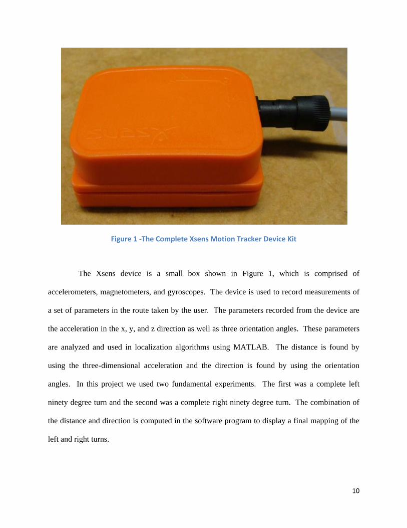
Table of Figures Figure 1 -The Complete Xsens Motion Tracker Device Kit .......................................................................... 10
Figure 2 - Angle of Arrival Geolocation Technique ..................................................................................... 16
Figure 3 - Direction Based Geolocation Technique ..................................................................................... 18
Figure 4 - MTx System Overview ................................................................................................................ 22
Figure 5 - MTx with Sensor-fixed Coordinate System Overlaid .................................................................. 26
Figure 6 -Device Coordinate Reference Frame versus Earth Fixed Reference Coordinate Frame ............. 27
Figure 7 - three Dimensional Orientation Output ...................................................................................... 28
Figure 8 -The fixed coordinate system of Euler Angles ............................................................................... 29
Figure 9 - MTx Motion Tracker Setup ......................................................................................................... 34
Figure 10 – MT Manager Output Sample ................................................................................................... 35
Figure 11 - Sample Display of Measurement Values .................................................................................. 36
Figure 12 - Routes of Experiments .............................................................................................................. 38
Figure 13 – Acceleration vs Time for Left Turn Experiment ....................................................................... 40
Figure 14 - Acceleration vs Time for Right Turn Experiment ...................................................................... 41
Figure 15 - Euler Angles vs Time for Left Turn Experiment ......................................................................... 42
Figure 16 - Euler Angles vs Time for Right Turn Experiment ...................................................................... 43
Figure 17 - Velocity vs Time for Left Turn Experiment................................................................................ 44
Figure 18 - Velocity vs Time for Right Turn Experiment ............................................................................. 45
Figure 19 – Distance vs Time for Left Turn Experiment .............................................................................. 46
Figure 20 - Distance vs Time for Right Turn Experiment ............................................................................ 47
Figure 21 – Final Mapping for Left Turn Experiment .................................................................................. 48
Figure 22 – Final Mapping for Right Turn Experiment ................................................................................ 49
7
1. Introduction
In today‟s world, technology is constantly being developed to better suit the everyday
lives of people. A field of technology that is rapidly gaining interest and being further
researched and explored is wireless systems. Wireless systems are enabled to allow a wireless
network to be expanded using multiple access points without the need for a wired connection to
connect them as was required in the past. As we look to the future, most industries perceive
wireless networks as a form of communication that is necessary for further advancement.
Wireless geolocation is the term used to refer to a system put in place to provide mobile
users with access to their location or position. Indoor geolocation is the method of tracking
navigation of an electronic device that is indoors. Indoor geolocation is mainly used to locate
people and property within buildings for emergency purposes. The personal locator services
locate a person‟s position and the locator device locates property. There are many outdoor
geolocation applications that have been introduced which provide mapping services such as
directions and information services such as traffic flow or the weather. The most commonly
used geolocation technology is the GPS.
1.1 Motivations for the Project
Global Positioning System (GPS) is a recent breaking technology that is a part of the
wireless field. GPS uses a constellation of twenty-four medium Earth orbit satellites that
transmit precise microwave signals that enable receivers to determine its location, time, and
velocity. Today‟s society is very dependent on GPS to determine location and its users vary
from domestic, commercial and military industries. Though GPS is very effective and has been
very successful, there is one thing this technology currently lacks which is deemed necessary to a
8
large market of users. This inefficiency is its ability to determine location within buildings. A
navigation system that locates its users indoors is valuable to people with impaired vision,
hospitals needing to locate equipment, locating children and firefighters during rescues as well as
other emergency responders. For this purpose, it is very important to find a method for
evaluating indoor geolocation and the concept of localization may be applicable to the devices
that strive to determine location in unknown surroundings. Localization is the technique using
computer software to determine location of an electronic device or transceiver wireless
transceiver.
The limitation of outdoor geolocation technologies such as GPS is the main motivation
for indoor geolocation development. Ultimately, developing an application that is combined
with GPS to provide both indoor and outdoor location tracking fulfills the location need. To
indicate the path of an electronic device indoors, we use inertial systems. An inertial system is a
navigation tool that uses the aid of a computer to detect location by gathering data without the
use of external sources. An inertial system seeks to aid those in adapting to unfamiliar
environments
Wireless geolocation is acquainted with emergency services because currently it is the
main market that seeks a device with technology that locates people or property that is indoors.
The system architecture of geolocation consists of a service provider which gives the location
information and location aware services to subscribers. The service provider contacts a location
control center which figures out the coordinates of a mobile station. The location control center
collects the information required to calculate the mobile stations location using parameters such
as received signal strength (RSS), angle of arrival (AOA), carrier signal phase of arrival (POA)
9
and time of arrival (TOA) of signals. The location control center is then able to determine the
location of the mobile to the service provider which visually displays the location to the user.
1.2 Description of the Project
In a progression targeted to developing the area of wireless geolocation to access the
needs of the emergency services market, the company Xsens has developed a product known as
the MTx Motion Tracker technology. The project focuses on using MTx in indoor geolocation
through the use of inertial sensing for orientation tracking. One of the major applications of
MTx is to develop the Navshoe technology. “The Navshoe system is able to navigate its users in
arbitrary environments with or without the use of GPS by using a miniature inertial or
magnetometer package wirelessly coupled to a PDA”.1 The MTx technology produces data that
can be used to tabulate the orientation of its user through its small wireless inertial sensor. It can
be further integrated with GPS for the use of location tracking in outdoor areas.
The goal of this major qualifying project was two-fold. The first part was to research,
explore and investigate the characteristics of the Xsens Motion Tracker device for indoor
geolocation. The second part was to use the knowledge gained from the research of the
technology to create a test-bed for the information collected from the MTx. This information
collected are parameters used to test for performance evaluation of the device and our
algorithms. This test-bed collects field data that is then processed by MATLAB codes to
determine the coordinates and evaluate its accuracy in relative positioning.
1 Moving Mixed Reality into the Real World – Pedestrian Tracking with Shoe-Mounted Inertial
Sensors, Eric Foxlin, November/December 2005, Page 1.
10
Figure 1 -The Complete Xsens Motion Tracker Device Kit
The Xsens device is a small box shown in Figure 1, which is comprised of
accelerometers, magnetometers, and gyroscopes. The device is used to record measurements of
a set of parameters in the route taken by the user. The parameters recorded from the device are
the acceleration in the x, y, and z direction as well as three orientation angles. These parameters
are analyzed and used in localization algorithms using MATLAB. The distance is found by
using the three-dimensional acceleration and the direction is found by using the orientation
angles. In this project we used two fundamental experiments. The first was a complete left
ninety degree turn and the second was a complete right ninety degree turn. The combination of
the distance and direction is computed in the software program to display a final mapping of the
left and right turns.
11
By analyzing the data recorded by the device, creating algorithms and using software
programming, this project showed through the creation of a test-bed and its results that there is
the potential of using the MTx to track a person‟s location inside a building.
1.3 Structure of the Project Report
This project aims to expand on inertial systems and consists of an in depth investigation
of the MTx Motion Tracker and analysis of the data obtained from the device. The following
chapters of the report involve an explanation of the sequence of steps taken in the project in
achieving the objectives.
The second chapter introduces the readers to localization and the challenges of the
industry by defining outdoor and indoor geolocation. It expresses reasons for a development in
this field and the markets it will affect. It gives the system architecture of geolocation and
methods to determining a user‟s position. These methods are the techniques that calculate
positioning of an electronic device such as a mobile telephone.
The third chapter gives a complete overview of the Xsens Motion Tracker. It defines
the components that the device is made up of and the functions of each component in the device.
It includes descriptions of the parameters used and how they must be calibrated when being
applied to this project.
The fourth chapter shows the test-bed developed to analyze the device. It consists of
the output of the device and understanding the output by doing other experiments. It also
introduces the two fundamental experiments that were used to evaluate the potential of the
device to aid in the indoor geolocation field.

12
The fifth chapter consists of the results of the test-bed. It gives the breakdown of each
step taken in producing the final mapping. It shows the graphs of each step and includes the
mathematical computation necessary to achieve the expected output.
The sixth and seventh chapter is the conclusion and future recommendations of the
project. It summarizes the entire project and its results as well as gives recommendations for
future work on this device.
13
2. Overview of Localization Techniques
The world has been exposed to and adapted to the use of outdoor geolocation in the form
of GPS and depend on it to determine information based on their location. The effectiveness of
GPS is very apparent outdoors but has weak or non-existent signal indoors. There are markets
that still require a device that can provide indoor geolocation. This has proved very challenging
and a number of technologies can be used for developing implementations.
This chapter introduces an overview of localization techniques. It addresses the
localization industry and its challenges, gives the system architecture, discusses performance
measure of geolocation and describes three techniques for determining positioning. These
techniques are direction-based, distance-based, and fingerprinting-based. The techniques are
also compared to decide on which ones are superior to the others.
2.1 The Localization Industry and its Challenges
Geolocation is the performance of accessing locations or gathering information to
calculate an estimation of a mobile station or position. Locating a user‟s position through means
of a wired connection is extremely fast because the position is easily identified with accuracy
due to the other rooms in the building. Locating users through means of a wireless connection is
more difficult because there is no fixed location for reference. It is very important to access ones
location in cases of emergency and because of this, wireless geolocation has gained significant
interest and numerous markets depend on its advancement for services.
Geolocation may be divided into two categories, indoor and outdoor geolocation. As the
name suggests, outdoor geolocation refers to wireless location outside and indoor geolocation
refers to wireless location within buildings. Outdoor geolocation is more common than indoor
14
geolocation and have introduced mapping services that entail giving directions or information
services that include traffic flow, etc. The most common outdoor geolocation application used is
the Global Positioning System that is installed in most cellular devices or automobiles being
made. While outdoor applications continue to grow, the need for a technology that gives
accurate location for indoor geolocation still exists.
Indoor geolocation aims to provide location for emergency services. There is a high
demand for indoor geolocation devices by emergency services market such as public safety,
nursing homes, visually impaired and children. The importance of such an application may be
seen in public safety that requires its location tracking indoors for firefighters. The police force
and fire fighters require a device that can locate victims within buildings. In the commercial
market, there is a need for a device that is able to track children or the elderly as well as an aid
for those with impaired vision or those that are blind for navigation purposes. There is also a
need for indoor location for hospitals or large corporations that require finding equipment at
critical times. However, despite the high demand for indoor tracking, there is still a lack of
applications to address this demand.
The system architecture of geolocation consists of a geolocation service provider, a
location control center, and a display system. Together these three systems combine information
gathered to produce a person‟s location visually. The geolocation service provider receives
information from the location control center to measure metrics relative to the position of the
mobile station to the reference point. The location control center collects the data needed to
work out the position of the mobile station. The data provided by the location control center is
the information for the positioning algorithm. This is the process of using metrics to determine
the location coordinate of the mobile station using angles of arrival (AOA), received signal
15
strength (RSS), phase of arrival (POA), and time of arrival (TOA). After the location is
determined and sent to the service provider, the mobile stations location is visually displayed to
the user through means of the display system.
The location control center is the „brain‟ of the geolocation system architecture that
calculates an estimation of location using metrics to determine methods to develop a user‟s
position. These methods are classified under three categories; Direction-Based Techniques,
Distance-Based Techniques and Fingerprinting-Based Techniques.
2.1.1 Direction-Based Techniques
The direction-based technique consists of the Angle of Arrival Method (AOA) which
uses the Ling of Sight (LOS) approach.
Angle of Arrival
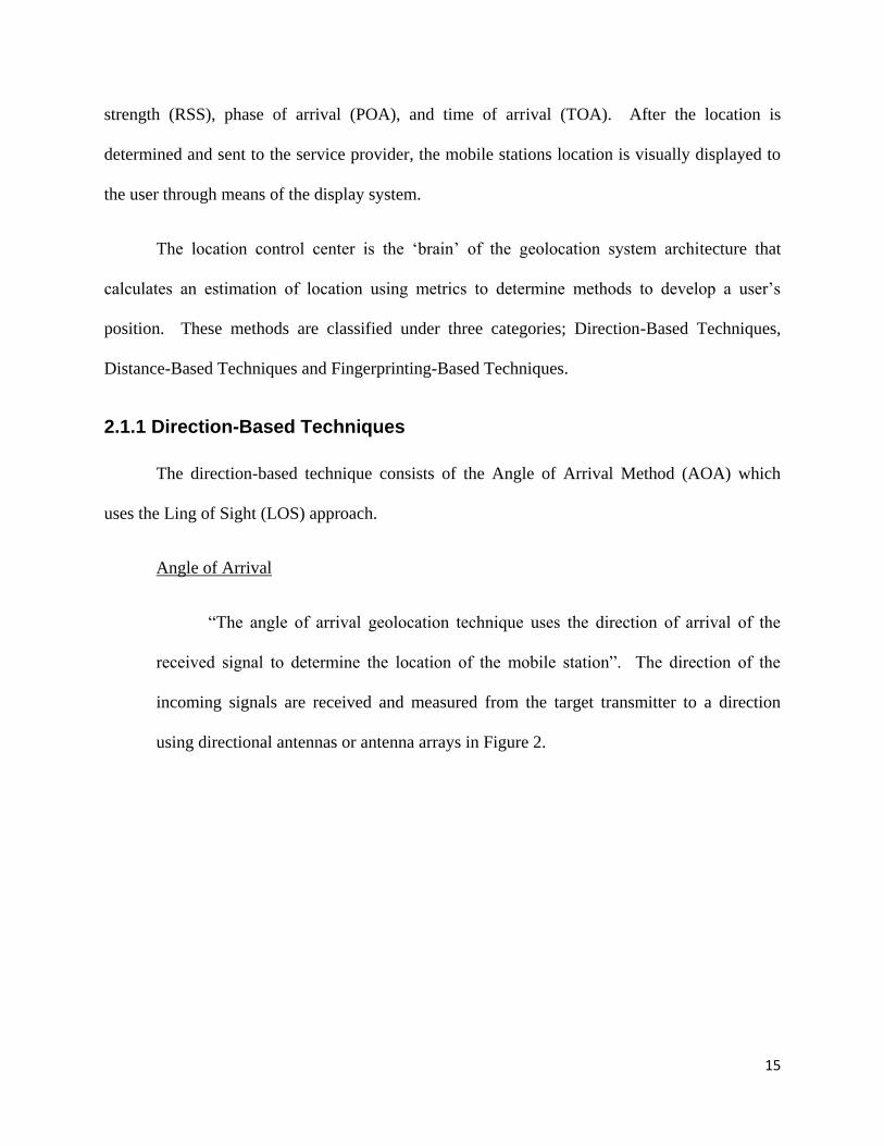
“The angle of arrival geolocation technique uses the direction of arrival of the
received signal to determine the location of the mobile station”. The direction of the
incoming signals are received and measured from the target transmitter to a direction
using directional antennas or antenna arrays in Figure 2.
16
Figure 2 - Angle of Arrival Geolocation Technique
If the line of sight signal path is blocked, then the angle of arrival being used is a
reflected or scattered signal for its direction estimation. This technique is not feasible when
dealing with indoor geolocation because often times there will be walls or objects blocking the
line of sight signal path. To eliminate the blocking of the line of sight signal path, a very large
amount of array antennas would need to be placed at all the receivers to track the arrival signal
direction to ensure accuracy which is extremely expensive.
2.1.2 Distance-Based Techniques
The Distance-Based Techniques involve the following methods:
- Time of Arrival (TOA)
- Time Difference of Arrival (TDOA)
17
- Signal Strength
- Received Signal Phase
Time of Arrival
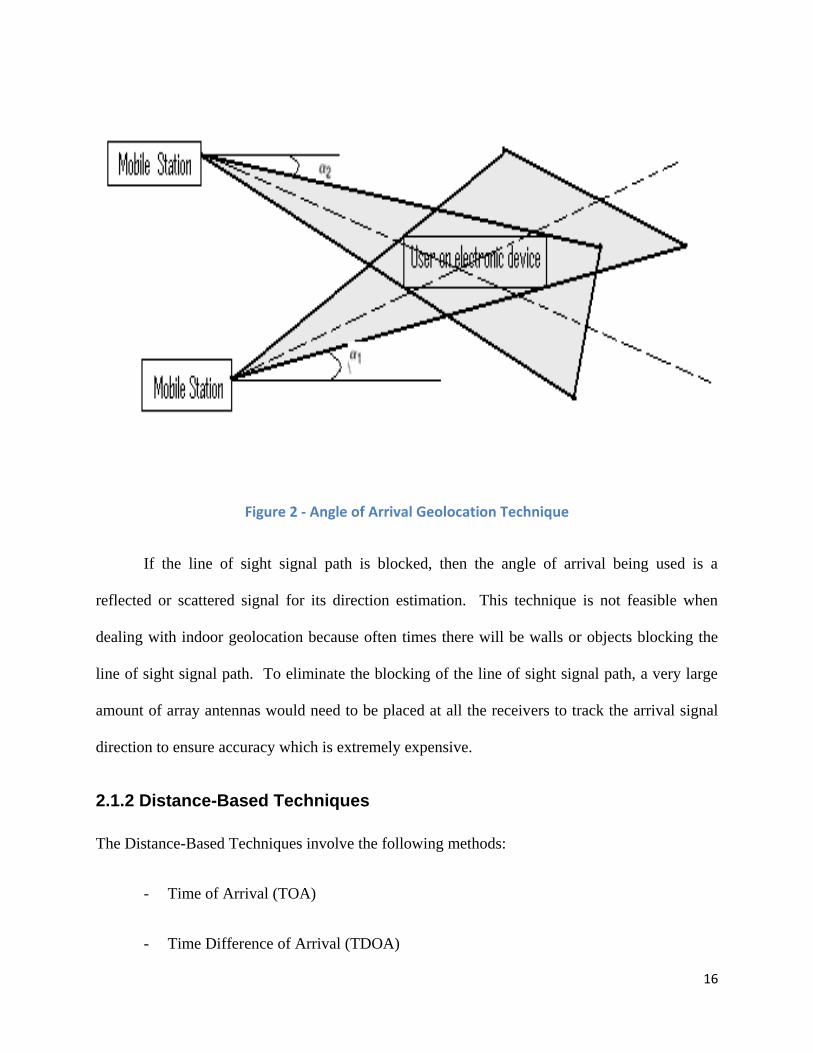
The time of arrival technique uses the distance between the mobile station and
receiver to estimate location. At least three measurements are necessary to calculate the
possible position of the user. The measurements estimate the position in two dimensions
and four measurements estimate the position in three dimension. By estimating the
distance between the receiver and the mobile to be d, the mobile is located on a circle
with radius d centered on the receiver. Distance is equal to the velocity of light
multiplied by the time taken by the signal to reach the base station. (d = c * t; where c is
the velocity of light and t is the time taken by the signal to reach the base station) Three
measurements of d provide a location of the mobile accurately as seen in Figure 3.
18
Figure 3 - Direction Based Geolocation Technique
Time Difference of Arrival
Some outdoor geolocation applications use the time difference of arrival
technique. This is where the differences of the time of arrivals are use to locate the
mobile. “The time difference of arrival technique is similar to that of the time of arrival
technique but instead of using circles, the time difference of arrival uses hyperbolas on
which the transmitter must be located with foci at the receivers”. 2 At least three
measurements are needed to calculate a fixed position at the intersection of the
hyperbolas.
2 Principles of Wireless Networks, Kaveh Pahlavan, Prashant Krishnamurthy, Wireless Geolocation Systems Chapter 14, Page 540.
19
Signal Strength
The signal strength technique uses the transmitted power at the mobile station and
the received signal strength at the base station to provide an estimate of the distance
between the transmitter and the receiver. Similar to the time of arrival technique, the
distance gives the circle centered on the receiver which the mobile transmitter is on.
Received Signal Phase
“The received signal phase technique used with reference receivers measures the
carrier phase. Differential Global Positioning System improves location accuracy within
twenty meters to one meter as compared with Global Positioning Systems which uses
range measurements. In indoor geolocation systems, it is possible to use signal phase
methods with time of arrival, time difference of arrival or received signal strength
techniques to better estimate the location.
2.1.3 Fingerprinting-Based Techniques
Another technique that estimates position location is signal fingerprinting. “The
multipath structure of the channel is unique to every location and may be considered a
„fingerprint‟ or „signature‟ of the location if the same radio frequency signal is transmitted from
that location. This technique may be used in indoor geolocation applications where a location
pattern develops from multipath rays in a multipath structure in an area”3.
3 Principles of Wireless Networks, Kaveh Pahlavan, Prashant Krishnamurthy, Wireless Geolocation Systems Chapter 14, Page 545.
20
2.2 Performance Measures of Geolocation Systems
“The performances of geolocation systems are tested on similar criterion as
telecommunication systems. The most important performance measure for a geolocation system
to be successful is accuracy of the location defined. The accuracy of the system may include the
percentage of calls within an accuracy of 8 meters or the distribution of distance error at the
receiver. The location availability of a system is important because it includes the percent of
location requests not fulfilled and the unacceptable uncertainty of locations. Other categories
used to determine the performance measurement of geolocation systems are the coverage of the
system, the reliability of the system and the delay in location computation”4.
2.3 Comparing Geolocation Techniques
The time of arrival technique estimate location by calculating the position of the mobile
by using circles centered on the mobile or the fixed transceiver. The time difference of arrival
does a similar technique using hyperbolas and does not require the knowledge of transmit time
from the transmitter. To create estimates of time, TOA and TDOA techniques employ pulse
transmission, phase information, or spread spectrum to arrive at locations of mobile stations.
The time of arrival techniques are seen as superior to angle of arrival techniques because
the AOA method is not appropriate for indoor geolocation systems. The angle of arrival is suited
for outdoor geolocation but has poor accuracy. It has a low delay but may be costly due to the
need for antenna arrays that need to be installed in areas. The signal strength method cannot be
used in situations where the precision of the location needs to be within accuracy of a few
meters.
4 Principles of Wireless Networks, Kaveh Pahlavan, Prashant Krishnamurthy, Wireless Geolocation Systems Chapter 14, Page 547.
21
3. Principle of Operation of MTx Motion Tracking System
The limitation of GPS calls for an inertial system that is able to be used where GPS
becomes ineffective or fails. One such application that attempts to resolve the restriction of the
GPS technology is a motion tracking device developed by Xsens, a company in the Netherlands.
This device can be used in fields such as biomechanics, exercise and sports, virtual reality,
animation, and motion capture. It gathers and records data from which algorithms may be
created to produce an application to go hand in hand with GPS for tracking location indoors.
This chapter provides an in-depth description of the Xsens Motion Tracker and how it
works. It provides function descriptions for each component and how they work together to
deliver the data needed to calculate relative positioning. It includes the parameters recorded by
the device and the calculations that need to occur before using the data. This chapter concludes
with how these parameters are used in order to get a final mapping.
3.1 An Overview of Inertial Systems using the MTx System
The MTx is a miniature three-degrees-of-freedom (3DoF) inertial orientation tracker
device developed by Xsens Technologies. This tracker device is a measurement unit for
collecting dynamic movements. It provides three-dimension magnetometers which may be
viewed as a three dimensional compass with an embedded processor capable of calculating roll,
pitch and yaw in real time, as well as outputting three dimensional linear acceleration rate of turn
with use of a gyroscope and earth-magnetic field data.
The MTx device takes the signals of the rate gyroscopes, accelerometers and
magnetometers to calculate an accurate statistical optimal three dimensional orientation estimate
22
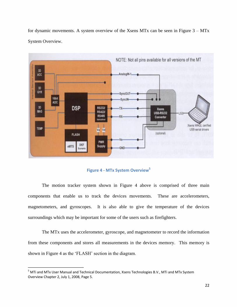
for dynamic movements. A system overview of the Xsens MTx can be seen in Figure 3 – MTx
System Overview.
Figure 4 - MTx System Overview5
The motion tracker system shown in Figure 4 above is comprised of three main
components that enable us to track the devices movements. These are accelerometers,
magnetometers, and gyroscopes. It is also able to give the temperature of the devices
surroundings which may be important for some of the users such as firefighters.
The MTx uses the accelerometer, gyroscope, and magnetometer to record the information
from these components and stores all measurements in the devices memory. This memory is
shown in Figure 4 as the „FLASH‟ section in the diagram.
5 MTi and MTx User Manual and Technical Documentation, Xsens Technologies B.V., MTi and MTx System Overview Chapter 2, July 1, 2008, Page 5.
23
The ADC is the analog to digital converter. This converts the input analog voltage to a
digital number. This converter is shown as ‟16 bit ADC‟ in the system overview diagram.
The power supply is the source of power to load the device. It provides the energy to
power the components running in the device. It is shown as „PWR Supply‟ in the system
overview diagram.
The transceiver is a device that has a transceiver as well as a receiver. This allows for the
device to be connected and receive and send signals to the converter or straight to the computer
aid needed to use the motion tracker. It is viewed as „RS232/RS422/RS485 transceiver‟ in the
system overview diagram.
The digital signal processor is a microchip that is used to measure or process signals.
This component is seen as „DSP‟ on the system overview diagram. After uploading the
information the user is then able to manipulate their algorithm to process the data.
The accelerometers measure gravitational acceleration as well as the acceleration due to
the movement of the object with respect to its surroundings. An assumption that the device
makes is that on average the acceleration due to the movement is zero. The three dimensional
acceleration measurements recorded by the accelerometer in the x, y, and z direction is in respect
to the device‟s reference coordinate frame and will need to be converted to the Earth‟s fixed
reference coordinate. This acceleration is manipulated to calculate the distance of the recorded
data which is needed in the final computation of the devices movements.
In addition to the three accelerations in the x, y, and z direction, three orientation angles
are needed to calculate the positioning. They are known as Euler angles. These angles are
referred to as the roll, pitch and yaw. The roll is defined as the rotation around the x-axis from -
24
180º to 180º. The pitch is defined as the rotation around y-axis from -90º to 90º. The yaw is
defined as the rotation around the z-axis from -180º to 180º.
The magnetometers measure the Earth magnetic field. This means that it is similar to
treating it as a compass. Therefore, it stabilizes the heading (yaw). When the Earth magnetic
field is disturbed, the MTx will track the disturbance and include it in its estimation. But in case
of structural magnetic disturbance, a „new‟ local magnetic north will be used to compute the
yaw. The gyroscopes and the magnetometers measure the orientation angles.
To obtain orientation, the MTx uses the assumptions about the acceleration and the
magnetic field. Based on the application the device is used for, the characteristics of the
acceleration or magnetic field will differ. The device may be set for different scenario based on
the types of movement. The different scenarios are divided in „human‟, „machine‟ and „marine‟
types of motion. The MTx application for which our project focuses on is human motion.
For „human‟ type of motion, the scenario assumes that it is slower movements while also
capturing the magnetic disturbances typically for an indoor environment. „Machine‟ type of
motion includes scenarios where acceleration are slower and of longer periods of time than
acceleration of humans. These scenarios are designed for situations where the local earth
magnetic field is too distorted to be useful. To adjust to these situations, the „machine‟ type of
motion does not make use of the local earth magnetic field to obtain a heading estimate. Lastly,
the „marine‟ type of motion is used for low, long term accelerations and mild magnetic
disturbances.
25
3.2 The Motion Tracker Output
There are two main modes of output produced by the MTx. These methods of output are
the Orientation Output and the Calibrated Data Output. The two modes may be combined to
view orientation data and inertial data together.
3.2.1 Calibrated Data Coordinate System
The sensor readings given in the calibrated data are the accelerations (from the
accelerometer), the rate of turns (from the gyroscope), and the earth magnetic field (from the
magnetometer). The readings collected are in the right handed Cartesian coordinate system. The
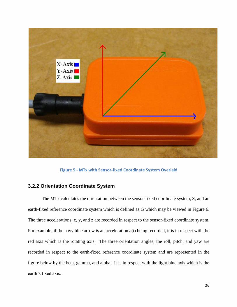
system is in three dimensions and is body-fixed to the device as seen in the Figure 5. The blue
arrow represents the x-axis, the yellow represents the y-axis and the green represents the z-axis.
The coordinate system is defined as the sensor coordinate system which is referred to as „S‟. The
three-dimensional output of the acceleration, the rate of turn, and the magnetic field data have
orthogonal XYZ readings within <0.1º.
26
Figure 5 - MTx with Sensor-fixed Coordinate System Overlaid
3.2.2 Orientation Coordinate System
The MTx calculates the orientation between the sensor-fixed coordinate system, S, and an
earth-fixed reference coordinate system which is defined as G which may be viewed in Figure 6.
The three accelerations, x, y, and z are recorded in respect to the sensor-fixed coordinate system.
For example, if the navy blue arrow is an acceleration a(t) being recorded, it is in respect with the
red axis which is the rotating axis. The three orientation angles, the roll, pitch, and yaw are
recorded in respect to the earth-fixed reference coordinate system and are represented in the
figure below by the beta, gamma, and alpha. It is in respect with the light blue axis which is the
earth‟s fixed axis.
27
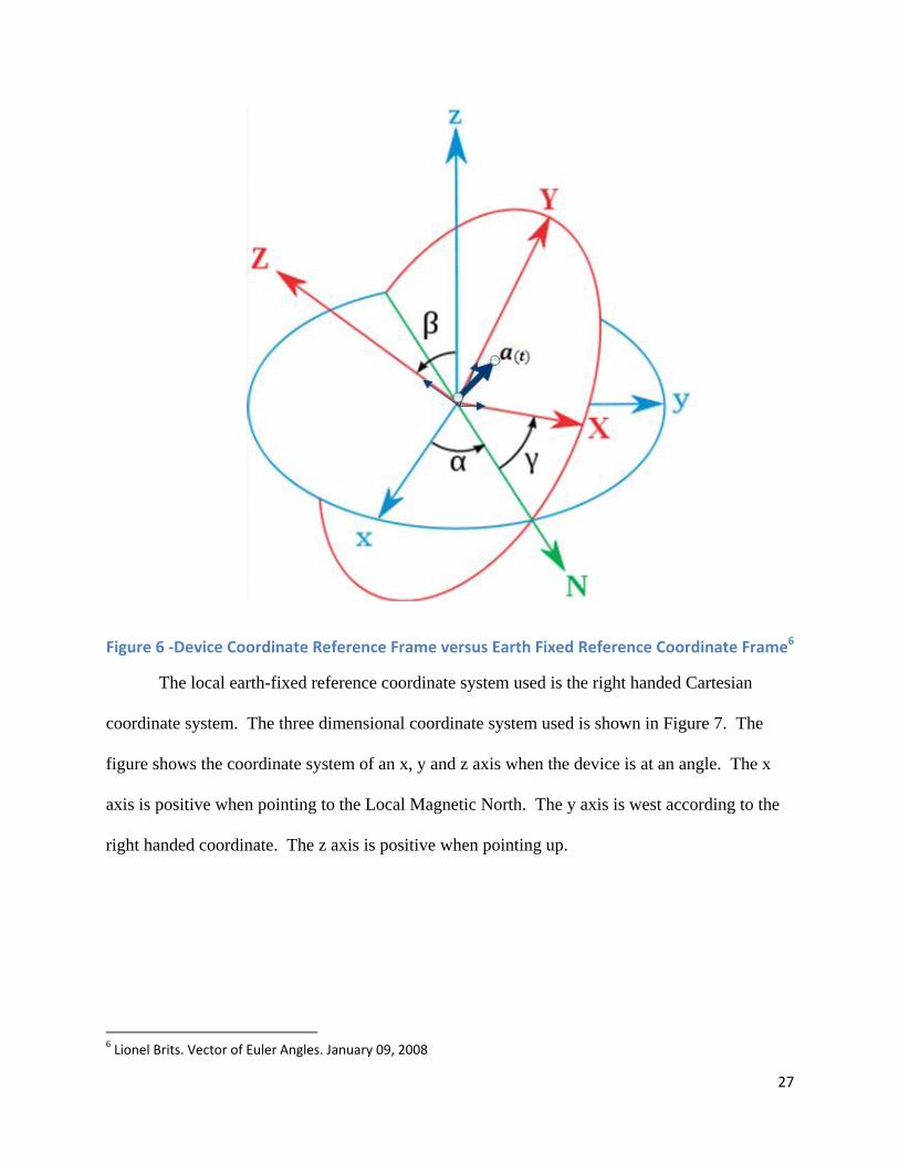
Figure 6 -Device Coordinate Reference Frame versus Earth Fixed Reference Coordinate Frame6
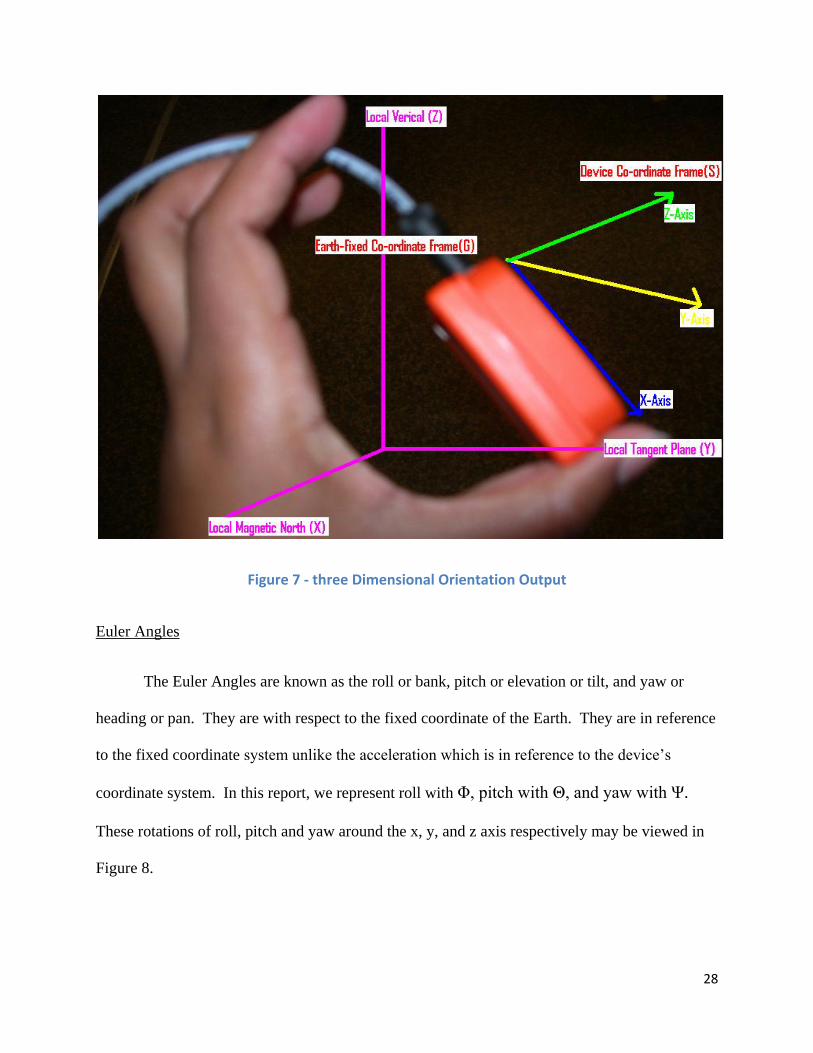
The local earth-fixed reference coordinate system used is the right handed Cartesian
coordinate system. The three dimensional coordinate system used is shown in Figure 7. The
figure shows the coordinate system of an x, y and z axis when the device is at an angle. The x
axis is positive when pointing to the Local Magnetic North. The y axis is west according to the
right handed coordinate. The z axis is positive when pointing up.
6 Lionel Brits. Vector of Euler Angles. January 09, 2008
28
Figure 7 - three Dimensional Orientation Output
Euler Angles
The Euler Angles are known as the roll or bank, pitch or elevation or tilt, and yaw or
heading or pan. They are with respect to the fixed coordinate of the Earth. They are in reference
to the fixed coordinate system unlike the acceleration which is in reference to the device‟s
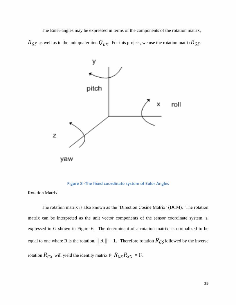
coordinate system. In this report, we represent roll with Φ, pitch with Θ, and yaw with Ψ.
These rotations of roll, pitch and yaw around the x, y, and z axis respectively may be viewed in
Figure 8.
29
The Euler-angles may be expressed in terms of the components of the rotation matrix,
𝑅𝐺𝑆 as well as in the unit quaternion 𝑄𝐺𝑆. For this project, we use the rotation matrix𝑅𝐺𝑆 .
Figure 8 -The fixed coordinate system of Euler Angles
Rotation Matrix
The rotation matrix is also known as the „Direction Cosine Matrix‟ (DCM). The rotation
matrix can be interpreted as the unit vector components of the sensor coordinate system, s,
expressed in G shown in Figure 6. The determinant of a rotation matrix, is normalized to be
equal to one where R is the rotation, || R || = 1. Therefore rotation 𝑅𝐺𝑆 followed by the inverse
rotation 𝑅𝐺𝑆 will yield the identity matrix I³, 𝑅𝐺𝑆𝑅𝑆𝐺 = I³.
30
Rotation Matrix expressed as Euler-Angles
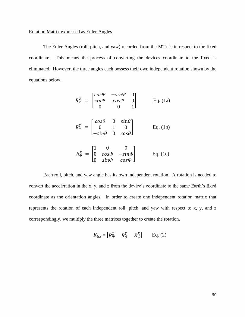
The Euler-Angles (roll, pitch, and yaw) recorded from the MTx is in respect to the fixed
coordinate. This means the process of converting the devices coordinate to the fixed is
eliminated. However, the three angles each possess their own independent rotation shown by the
equations below.
𝑅𝛹𝑍 =
𝑐𝑜𝑠𝛹 −𝑠𝑖𝑛𝛹 0𝑠𝑖𝑛𝛹 𝑐𝑜𝑠𝛹 0
0 0 1 Eq. (1a)
𝑅𝜃𝑌 =
𝑐𝑜𝑠𝜃 0 𝑠𝑖𝑛𝜃0 1 0
−𝑠𝑖𝑛𝜃 0 𝑐𝑜𝑠𝜃 Eq. (1b)
𝑅𝛷𝑋 =
1 0 00 𝑐𝑜𝑠𝛷 −𝑠𝑖𝑛𝛷0 𝑠𝑖𝑛𝛷 𝑐𝑜𝑠𝛷
Eq. (1c)
Each roll, pitch, and yaw angle has its own independent rotation. A rotation is needed to
convert the acceleration in the x, y, and z from the device‟s coordinate to the same Earth‟s fixed
coordinate as the orientation angles. In order to create one independent rotation matrix that
represents the rotation of each independent roll, pitch, and yaw with respect to x, y, and z
correspondingly, we multiply the three matrices together to create the rotation.
𝑅𝐺𝑆 = 𝑅𝛹𝑍 𝑅𝜃
𝑌 𝑅𝛷𝑋 Eq. (2)
31
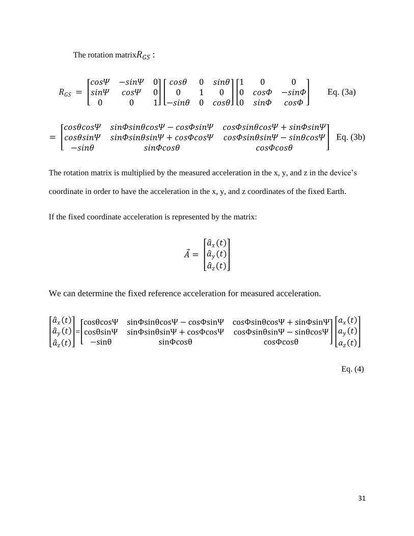
The rotation matrix𝑅𝐺𝑆 :
𝑅𝐺𝑆 = 𝑐𝑜𝑠𝛹 −𝑠𝑖𝑛𝛹 0𝑠𝑖𝑛𝛹 𝑐𝑜𝑠𝛹 0
0 0 1
𝑐𝑜𝑠𝜃 0 𝑠𝑖𝑛𝜃0 1 0
−𝑠𝑖𝑛𝜃 0 𝑐𝑜𝑠𝜃
1 0 00 𝑐𝑜𝑠𝛷 −𝑠𝑖𝑛𝛷0 𝑠𝑖𝑛𝛷 𝑐𝑜𝑠𝛷
Eq. (3a)
= 𝑐𝑜𝑠𝜃𝑐𝑜𝑠𝛹 𝑠𝑖𝑛𝛷𝑠𝑖𝑛𝜃𝑐𝑜𝑠𝛹 − 𝑐𝑜𝑠𝛷𝑠𝑖𝑛𝛹 𝑐𝑜𝑠𝛷𝑠𝑖𝑛𝜃𝑐𝑜𝑠𝛹 + 𝑠𝑖𝑛𝛷𝑠𝑖𝑛𝛹𝑐𝑜𝑠𝜃𝑠𝑖𝑛𝛹 𝑠𝑖𝑛𝛷𝑠𝑖𝑛𝜃𝑠𝑖𝑛𝛹 + 𝑐𝑜𝑠𝛷𝑐𝑜𝑠𝛹 𝑐𝑜𝑠𝛷𝑠𝑖𝑛𝜃𝑠𝑖𝑛𝛹 − 𝑠𝑖𝑛𝜃𝑐𝑜𝑠𝛹−𝑠𝑖𝑛𝜃 𝑠𝑖𝑛𝛷𝑐𝑜𝑠𝜃 𝑐𝑜𝑠𝛷𝑐𝑜𝑠𝜃
Eq. (3b)
The rotation matrix is multiplied by the measured acceleration in the x, y, and z in the device‟s
coordinate in order to have the acceleration in the x, y, and z coordinates of the fixed Earth.
If the fixed coordinate acceleration is represented by the matrix:
𝐴 =
𝑎 𝑥(𝑡)𝑎 𝑦(𝑡)
𝑎 𝑧(𝑡)
We can determine the fixed reference acceleration for measured acceleration.
𝑎 𝑥 𝑡
𝑎 𝑦 𝑡
𝑎 𝑧 𝑡
= cosθcosΨ sinΦsinθcosΨ − cosΦsinΨ cosΦsinθcosΨ + sinΦsinΨcosθsinΨ sinΦsinθsinΨ + cosΦcosΨ cosΦsinθsinΨ − sinθcosΨ−sinθ sinΦcosθ cosΦcosθ
𝑎𝑥 𝑡
𝑎𝑦 𝑡
𝑎𝑧 𝑡
Eq. (4)
32
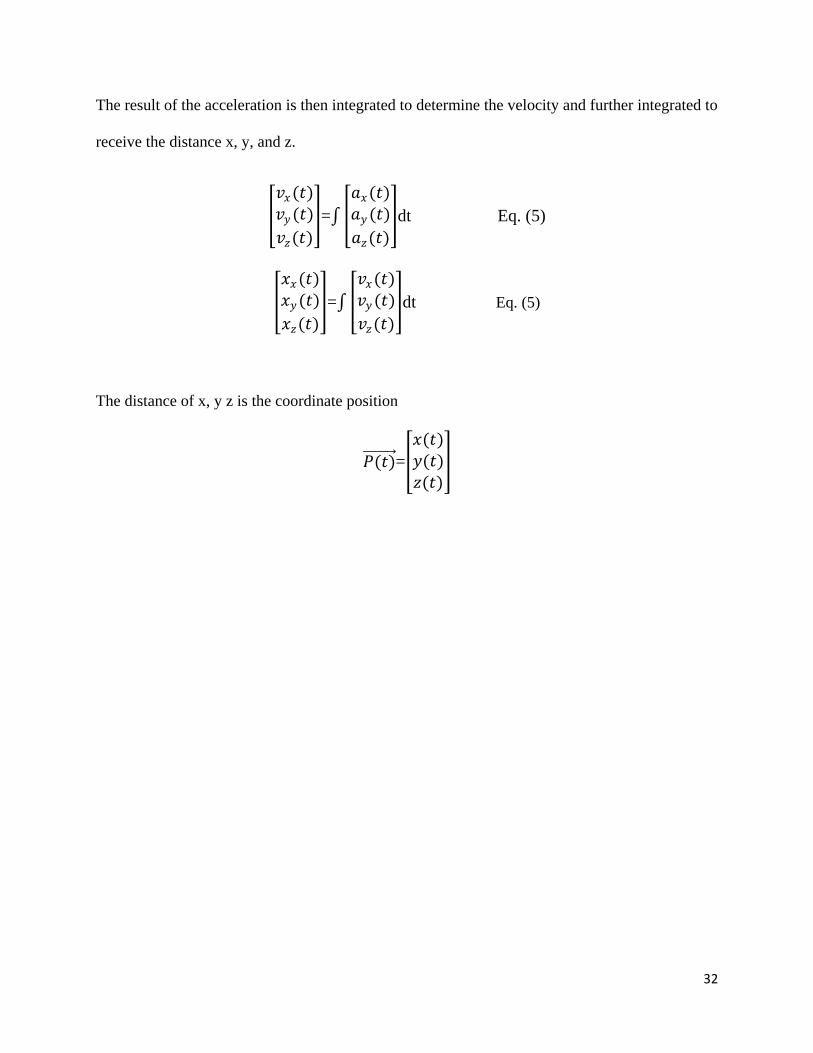
The result of the acceleration is then integrated to determine the velocity and further integrated to
receive the distance x, y, and z.
𝑣𝑥(𝑡)𝑣𝑦(𝑡)
𝑣𝑧(𝑡)
=
𝑎𝑥(𝑡)𝑎𝑦(𝑡)
𝑎𝑧(𝑡)
dt Eq. (5)
𝑥𝑥(𝑡)𝑥𝑦(𝑡)
𝑥𝑧(𝑡)
=
𝑣𝑥(𝑡)𝑣𝑦(𝑡)
𝑣𝑧(𝑡)
dt Eq. (5)
The distance of x, y z is the coordinate position
𝑃(𝑡) =
𝑥(𝑡)𝑦(𝑡)𝑧(𝑡)
33
4. Exploration and Test of MTx Motion Tracker
MTx Motion Tracker is a complex system. In this chapter, we first reported the
exploration of the characteristics of the MTx Technology. Then, we discussed the test-bed that
was developed for performance evaluation to determine the precision of the MTx Motion
Tracker Technology for indoor geolocation.
4.1 Exploration of the MTx Technology
The research section was divided into two parts. First, we explored the all available
information about the inertial system technology. Then, we worked on to familiarize the
components and functions of the miniature three-degrees-of-freedom MTx inertial orientation
tracker. By completing this, we achieved an in-depth understanding of the characteristics of this
technology.
4.1.1 Previous Work
Inertial system technology is in a developing stage for indoor geolocation. Previous
journals, reports, and other published articles are available to read and were ready to be
expanded upon. These previous work explained this new technology in depth and the
experiments that were ran. We took the information and used it to grasp a better understanding
for this project. These published materials can be found in our reference section.
4.1.2 Understanding of the MTx Motion Tracker
The next step was to get familiarize with the MTx Motion Tracker from Xsens
Technologies. To achieve this step, multiple experiments were run from the MTx device to attain
34
the output data and functions of the motion tracker. Along with the help of the provided MTx
user manual, the experimental observations were made comprehensible.
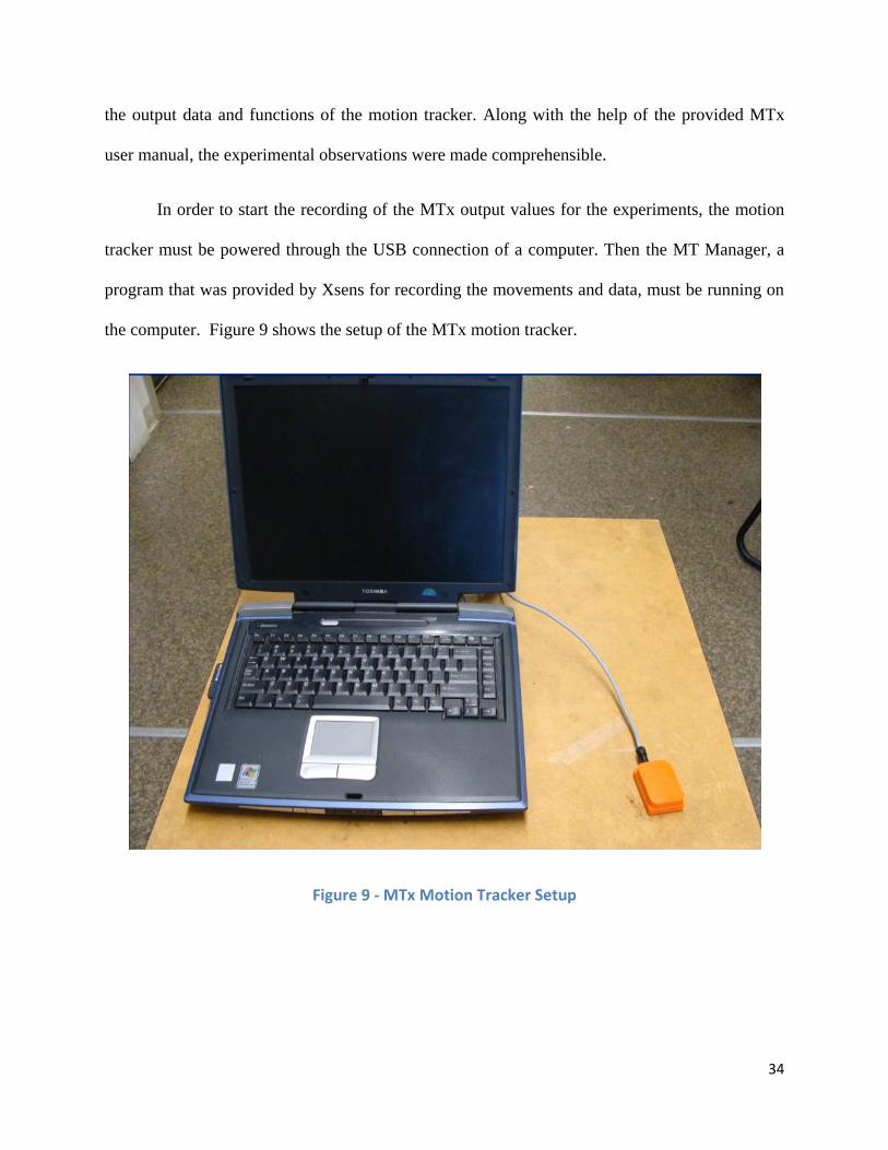
In order to start the recording of the MTx output values for the experiments, the motion
tracker must be powered through the USB connection of a computer. Then the MT Manager, a
program that was provided by Xsens for recording the movements and data, must be running on
the computer. Figure 9 shows the setup of the MTx motion tracker.
Figure 9 - MTx Motion Tracker Setup
35
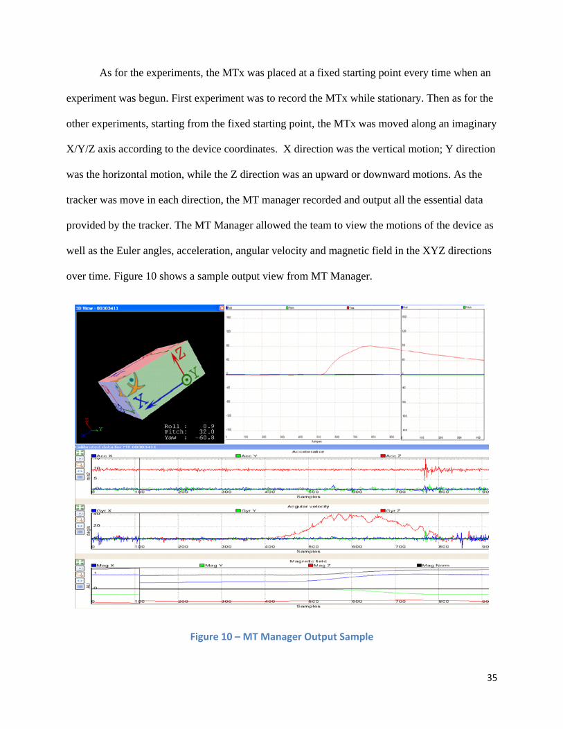
As for the experiments, the MTx was placed at a fixed starting point every time when an
experiment was begun. First experiment was to record the MTx while stationary. Then as for the
other experiments, starting from the fixed starting point, the MTx was moved along an imaginary
X/Y/Z axis according to the device coordinates. X direction was the vertical motion; Y direction
was the horizontal motion, while the Z direction was an upward or downward motions. As the
tracker was move in each direction, the MT manager recorded and output all the essential data
provided by the tracker. The MT Manager allowed the team to view the motions of the device as
well as the Euler angles, acceleration, angular velocity and magnetic field in the XYZ directions
over time. Figure 10 shows a sample output view from MT Manager.
Figure 10 – MT Manager Output Sample
36
As seen on the last page, there is a live 3D view of the device with the roll, pitch and yaw
rotational measurements in degrees. The plots also run live so that the output from the
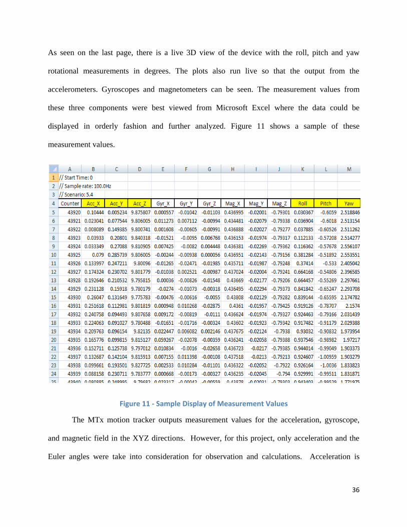
accelerometers. Gyroscopes and magnetometers can be seen. The measurement values from
these three components were best viewed from Microsoft Excel where the data could be
displayed in orderly fashion and further analyzed. Figure 11 shows a sample of these
measurement values.
Figure 11 - Sample Display of Measurement Values
The MTx motion tracker outputs measurement values for the acceleration, gyroscope,
and magnetic field in the XYZ directions. However, for this project, only acceleration and the
Euler angles were take into consideration for observation and calculations. Acceleration is
37
measured in m/sec² while the Euler angles units are in degrees. With the different experiments
output data, we compared and contrasted them from each direction to the stationary sample. By
doing this, the team was able to observe the following characteristics:
The duration of the test run was discovered by using simple computation. Time was
calculated by the total number of points divided by the tracker‟s set frequency of 100Hz.
The unit for time is seconds.
Acceleration in the Z direction was within the range of 9.78 and 9.82 m/s² when the
motion tracker was not moved in that direction. This is around the Earth gravitational
acceleration constant of 9.81 m/s².
Yaw has a change of 90 degrees when the MTx device is rotate left or right. +90 for left
turn and -90 for a right turn.
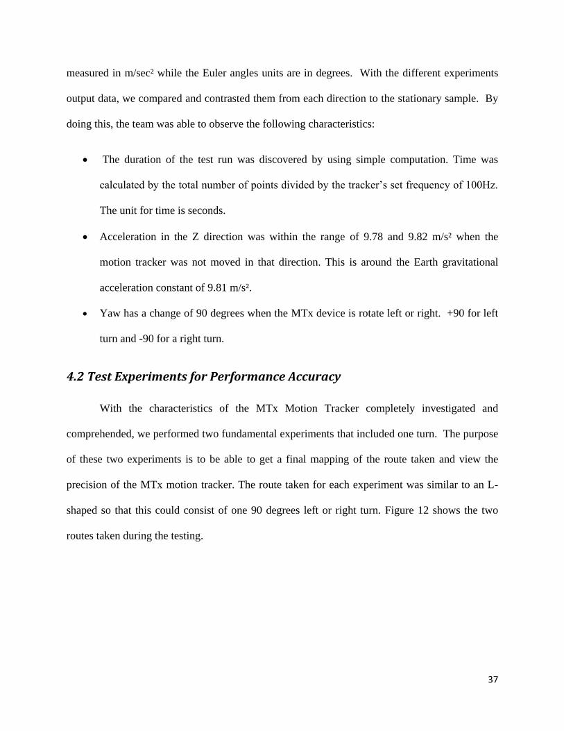
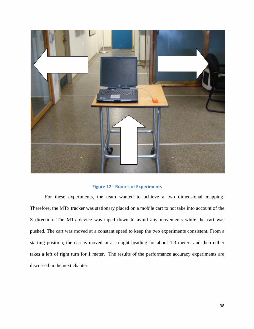
4.2 Test Experiments for Performance Accuracy
With the characteristics of the MTx Motion Tracker completely investigated and
comprehended, we performed two fundamental experiments that included one turn. The purpose
of these two experiments is to be able to get a final mapping of the route taken and view the
precision of the MTx motion tracker. The route taken for each experiment was similar to an L-
shaped so that this could consist of one 90 degrees left or right turn. Figure 12 shows the two
routes taken during the testing.
38
Figure 12 - Routes of Experiments
For these experiments, the team wanted to achieve a two dimensional mapping.
Therefore, the MTx tracker was stationary placed on a mobile cart to not take into account of the
Z direction. The MTx device was taped down to avoid any movements while the cart was
pushed. The cart was moved at a constant speed to keep the two experiments consistent. From a
starting position, the cart is moved in a straight heading for about 1.3 meters and then either
takes a left of right turn for 1 meter. The results of the performance accuracy experiments are
discussed in the next chapter.
39
5. Experimental Results
In this chapter, we displayed the results from the 90 degrees left and right turns test
experiments described in chapter four. First, we changed the outputted data from device
coordinates to fixed coordinates. Then, we integrated the fixed data and the inertial localization
algorithm with MATLAB to determine the precision of the MTx device. Finally, we show the
final maps of these two experiments.
5.1 Device and Fixed Coordinates
The results of the taken routes were logged by the MTx program manager. The key
output data that was taken into account were the relative acceleration and the Euler angles, also
known as rotation of coordinates. The relative acceleration was given according to the device
coordinates. In order to attain the final mapping, the device coordinates had to be changed to
Earth fixed coordinates. Eq. (4) was used here to achieve the change. The relative acceleration is
multiplied by the rotational matrix to get the fixed acceleration. From there, further calculations
would be in the fixed coordinates.
5.2 Plots of Acceleration, Euler Angles, Velocity and Distance
The values in the fixed coordinates obtained were programmed and manipulated in
MATLAB to produce the display of data on two dimensional plots. The MATLAB code can be
found in the Appendix. The acceleration, the Euler angles, the computed velocity and distance
for both left and right turn experiments are shown and discussed in this section. The duration for
each of these experiments was around 17 seconds.
40
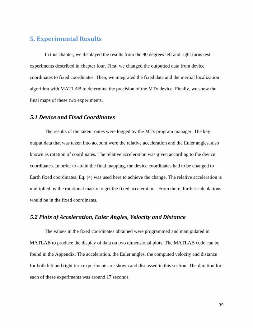
5.2.1 Acceleration
The acceleration data was changed from the device coordinates to the fixed coordinates.
The acceleration over time plots for left and right turns experiments are displayed below in
Figures 13 and 14, respectively.
Figure 13 – Acceleration vs Time for Left Turn Experiment
41
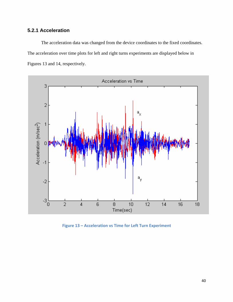
Figure 14 - Acceleration vs Time for Right Turn Experiment
These plots were obtained by taking the X and Y accelerations in the fixed coordinates
and plotted versus time. As you can see from the plots above, the MTx tracker is very sensitive
which causes lots of noise density to the data. The cart pushed starting around two seconds as the
XY acceleration spiked. Acceleration started to decrease as it approaches ten seconds because
the cart was making the turns. Around ten seconds, the spiked again as the cart started to be
pushed again in the new direction. This proves the MTx tracker is accurate in outputting the
acceleration data because the plots show the correct timing of the increased and decreased
acceleration from beginning to end.
42
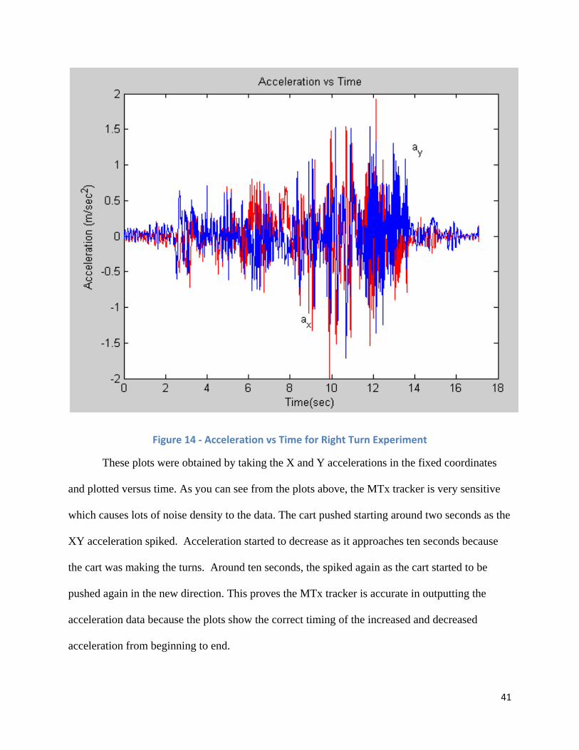
5.2.2 Euler Angles
The MTx tracker logs the roll, pitch, and yaw. These values are the Euler angles at which
the device rotates. The MATLAB software manipulates the values in order to obtain the angles at
which the user of the device is turning. Figures 15and 16, respectively, show the plots of the
roll, pitch and yaw degrees over time for the left and right turn experiments.
Figure 15 - Euler Angles vs Time for Left Turn Experiment
43
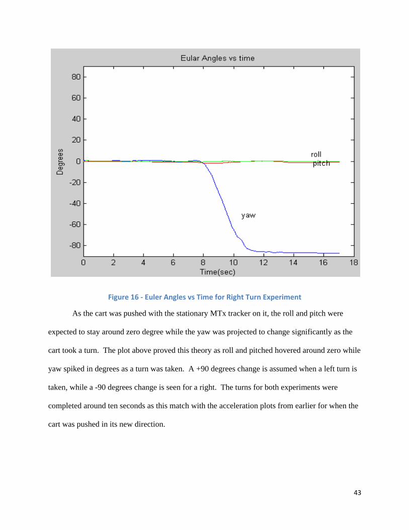
Figure 16 - Euler Angles vs Time for Right Turn Experiment
As the cart was pushed with the stationary MTx tracker on it, the roll and pitch were
expected to stay around zero degree while the yaw was projected to change significantly as the
cart took a turn. The plot above proved this theory as roll and pitched hovered around zero while
yaw spiked in degrees as a turn was taken. A +90 degrees change is assumed when a left turn is
taken, while a -90 degrees change is seen for a right. The turns for both experiments were
completed around ten seconds as this match with the acceleration plots from earlier for when the
cart was pushed in its new direction.
44
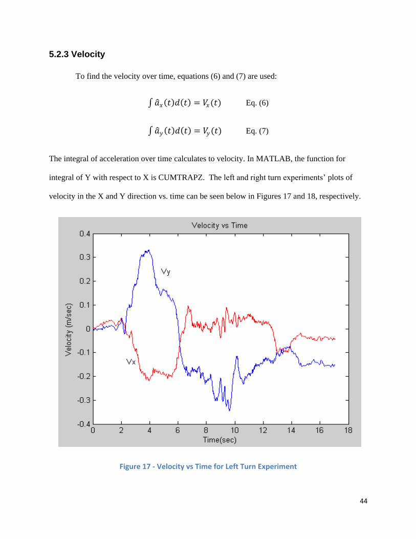
5.2.3 Velocity
To find the velocity over time, equations (6) and (7) are used:
𝑎 𝑥 𝑡 𝑑 𝑡 = 𝑉𝑥(𝑡) Eq. (6)
𝑎 𝑦 𝑡 𝑑 𝑡 = 𝑉𝑦(𝑡) Eq. (7)
The integral of acceleration over time calculates to velocity. In MATLAB, the function for
integral of Y with respect to X is CUMTRAPZ. The left and right turn experiments‟ plots of
velocity in the X and Y direction vs. time can be seen below in Figures 17 and 18, respectively.
Figure 17 - Velocity vs Time for Left Turn Experiment
45
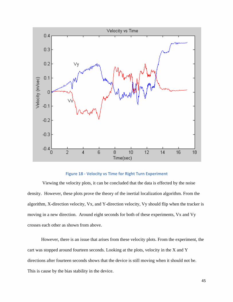
Figure 18 - Velocity vs Time for Right Turn Experiment
Viewing the velocity plots, it can be concluded that the data is effected by the noise
density. However, these plots prove the theory of the inertial localization algorithm. From the
algorithm, X-direction velocity, Vx, and Y-direction velocity, Vy should flip when the tracker is
moving in a new direction. Around eight seconds for both of these experiments, Vx and Vy
crosses each other as shown from above.
However, there is an issue that arises from these velocity plots. From the experiment, the
cart was stopped around fourteen seconds. Looking at the plots, velocity in the X and Y
directions after fourteen seconds shows that the device is still moving when it should not be.
This is cause by the bias stability in the device.
46
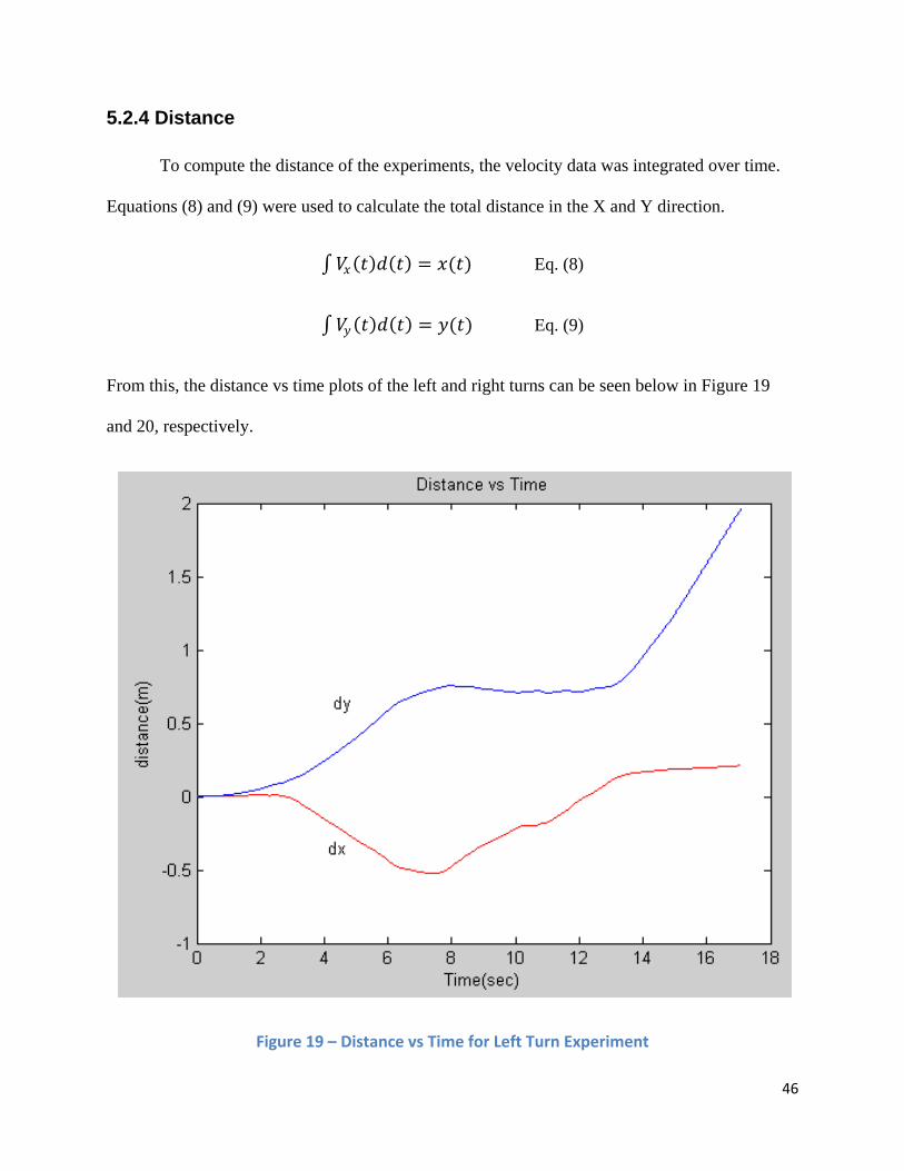
5.2.4 Distance
To compute the distance of the experiments, the velocity data was integrated over time.
Equations (8) and (9) were used to calculate the total distance in the X and Y direction.
𝑉𝑥 𝑡 𝑑 𝑡 = 𝑥(𝑡) Eq. (8)
𝑉𝑦 𝑡 𝑑 𝑡 = 𝑦(𝑡) Eq. (9)
From this, the distance vs time plots of the left and right turns can be seen below in Figure 19
and 20, respectively.
Figure 19 – Distance vs Time for Left Turn Experiment
47
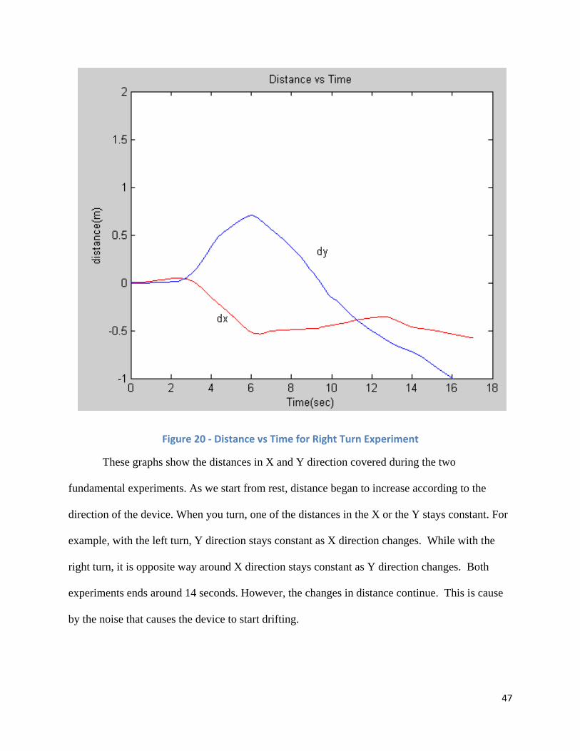
Figure 20 - Distance vs Time for Right Turn Experiment
These graphs show the distances in X and Y direction covered during the two
fundamental experiments. As we start from rest, distance began to increase according to the
direction of the device. When you turn, one of the distances in the X or the Y stays constant. For
example, with the left turn, Y direction stays constant as X direction changes. While with the
right turn, it is opposite way around X direction stays constant as Y direction changes. Both
experiments ends around 14 seconds. However, the changes in distance continue. This is cause
by the noise that causes the device to start drifting.
48
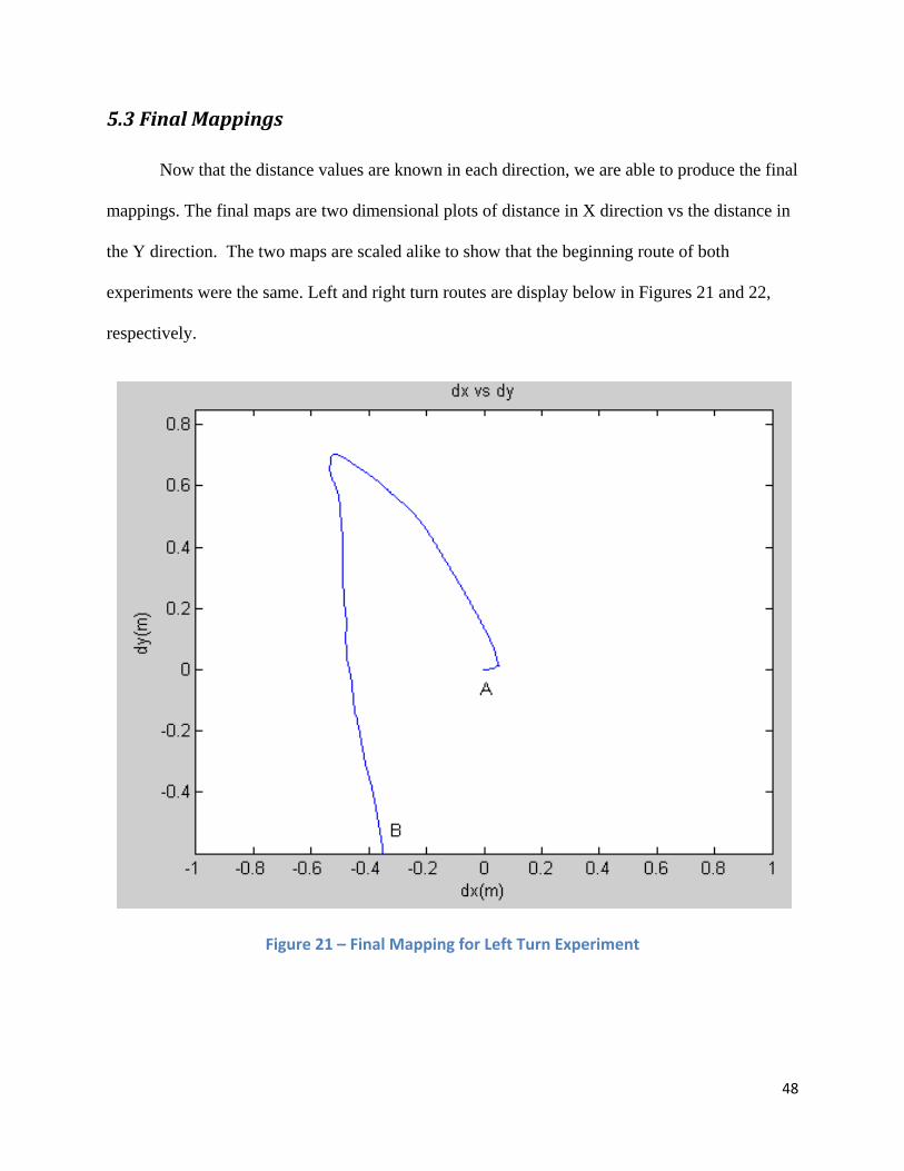
5.3 Final Mappings
Now that the distance values are known in each direction, we are able to produce the final
mappings. The final maps are two dimensional plots of distance in X direction vs the distance in
the Y direction. The two maps are scaled alike to show that the beginning route of both
experiments were the same. Left and right turn routes are display below in Figures 21 and 22,
respectively.
Figure 21 – Final Mapping for Left Turn Experiment
49
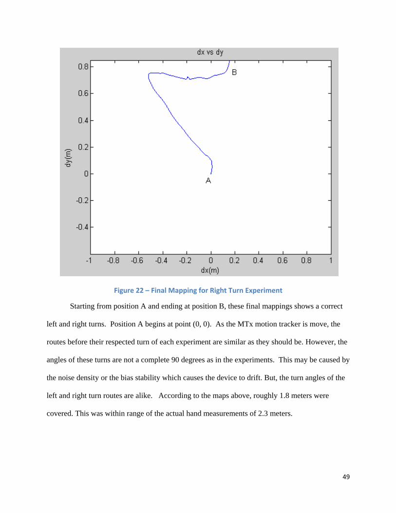
Figure 22 – Final Mapping for Right Turn Experiment
Starting from position A and ending at position B, these final mappings shows a correct
left and right turns. Position A begins at point (0, 0). As the MTx motion tracker is move, the
routes before their respected turn of each experiment are similar as they should be. However, the
angles of these turns are not a complete 90 degrees as in the experiments. This may be caused by
the noise density or the bias stability which causes the device to drift. But, the turn angles of the
left and right turn routes are alike. According to the maps above, roughly 1.8 meters were
covered. This was within range of the actual hand measurements of 2.3 meters.
50
6. Summary and Conclusion
In this project we researched and explored the characteristics of inertial systems using the
Xsens Motion Tracker device for indoor geolocation and created a test-bed to evaluate the
performance of the technology. The Xsens Motion Tracker attempts at providing an accurate
indoor geolocation technology by using inertial systems. The MTx is used to record and store
acceleration in the x, y, and z direction as well as the orientation angels, which are then used by
the team in algorithms to output an indoor displacement mapping of experiments.
The parameters used from the device were divided into acceleration in the x, y, z
direction and orientation angles. These two sets of information were found to be in respect to
two coordinate; the device‟s coordinate frame and the Earth‟s fixed coordinate frame. The three
dimensional acceleration is in respect to the device‟s coordinate frame system and the orientation
angles in respect to the Earth‟s fixed coordinate system. The acceleration in respect to time is
converted to the fixed coordinate by use of the rotation matrix. By multiplying the rotation
matrix with acceleration in the x, y and z direction in respect to time, the three dimension
acceleration vector in respect to time is produced. We then integrate the acceleration vector to
get the velocity vector with respect to time. This is followed by integrating the velocity vector
with respect to time to get the position vector with respect to time. This position vector is
combined with the orientation angles through software programming to produce a final mapping
of the test-bed.
The test-bed consisted of a fundamental experiment including a left 90 degree turn and a
right 90 degree turn. In each case, after testing using the procedure explained, the final mapping
51
showed the equivalent expected mapping of left and right turns. The angles of the two turns
were not complete 90 degrees but can be shown with further algorithm development.
Based on the device‟s performance and the inertial localization algorithms, we were able
to conclude that with further development in the algorithm to reduce noise, bias, or drifts, the
Xsens Motion Tracker device is marketable and may be effective where Global Positioning
Systems fail.
6.1 Future Recommendations
Outdoor localization is a well developed industry that global positioning systems is a
technology of which most are familiar with and has very popular usage. Its main downfall is that
it is very ineffective indoors. The indoor localization field is still in its process of development
and has a lack of applications committed to orientation tracking indoors. By continuing the
process of developing the inertial system for indoor localization using devices such as the Xsens
Motion Tracker and comparing it with other technologies such as Wi-Fi localization, the indoor
geolocation field continues to expand and may be integrated with outdoor localization
applications. Other recommendations that would benefit the industry are to integrate such an
application with GPS for both outdoor and indoor localization and to design hybrid localization
using inertial systems.
52
References
1. Xsens Technologies. “MTi and MTx User Manual and Technical Documentation”.
2. Eric Foxlin. “NavShoe™ Pedestrian Inertial Navigation Technology Brief”. 8/2006
http://www.ece.wpi.edu/Research/PPL/Workshops/2006/PDF/InterSense.pdf
3. Eric Foxlin. “Pedestrian Tracking with Shoe-Mounted Inertial Sensors”. 12/2005
4. Stephane Beauregard. “Omnidirectional Pedestrian Navigation for First Responders”.
53
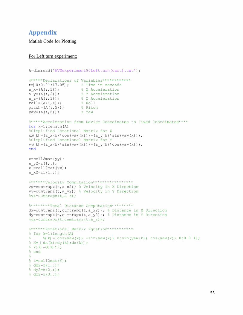
Appendix
Matlab Code for Plotting
For Left turn experiment:
A=dlmread('AVGexperiment90Leftturn(cart).txt');
%*****Declarations of Variables************ t=[0:0.01:17.05]; % Time in seconds a_x=(A(:,1)); % X Acceleration a_y=(A(:,2)); % Y Acceleration a_z=(A(:,3)); % Z Acceleration roll=(A(:,4)); % Roll pitch=(A(:,5)); % Pitch yaw=(A(:,6)); % Yaw
%*****Acceleration from Device Coordinates to Fixed Coordinates**** for k=1:length(A) %Simplified Rotational Matrix for X
xx{k}=(a_x(k)*cos(yaw(k)))+(a_y(k)*sin(yaw(k)));
%Simplified Rotational Matrix for Y
yy{k}=(a_x(k)*sin(yaw(k)))+(a_y(k)*cos(yaw(k))); end
z=cell2mat(yy); a_y2=z(1,:); z1=cell2mat(xx); a_x2=z1(1,:);
%******Velocity Computation***************** vx=cumtrapz(t,a_x2); % Velocity in X Direction vy=cumtrapz(t,a_y2); % Velocity in Y Direction %vz=cumtrapz(t,a_z);
%********Total Distance Computation********* dx=cumtrapz(t,cumtrapz(t,a_x2)); % Distance in X Direction dy=cumtrapz(t,cumtrapz(t,a_y2)); % Distance in Y Direction %dz=cumtrapz(t,cumtrapz(t,a_z));
%******Rotational Matrix Equation*********** % for k=1:length(A) % G{k}=[cos(yaw(k)) -sin(yaw(k)) 0;sin(yaw(k)) cos(yaw(k)) 0;0 0 1]; % H= [dx(k);dy(k);dz(k)]; % Y{k}=G{k}*H; % end % % z=cell2mat(Y); % dx2=z(1,:); % dy2=z(2,:); % dz2=z(3,:);
54
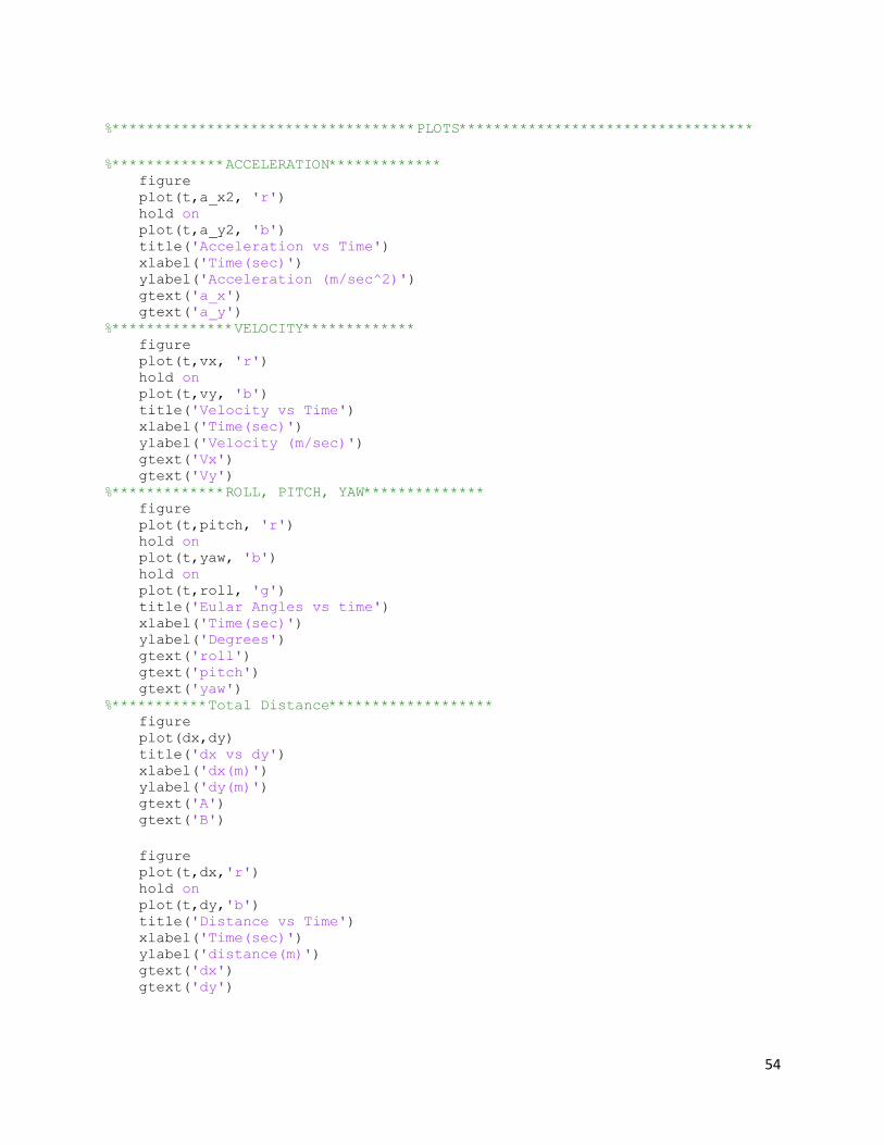
%***********************************PLOTS**********************************
%*************ACCELERATION************* figure plot(t,a_x2, 'r') hold on plot(t,a_y2, 'b') title('Acceleration vs Time') xlabel('Time(sec)') ylabel('Acceleration (m/sec^2)') gtext('a_x') gtext('a_y') %**************VELOCITY************* figure plot(t,vx, 'r') hold on plot(t,vy, 'b') title('Velocity vs Time') xlabel('Time(sec)') ylabel('Velocity (m/sec)') gtext('Vx') gtext('Vy') %*************ROLL, PITCH, YAW************** figure plot(t,pitch, 'r') hold on plot(t,yaw, 'b') hold on plot(t,roll, 'g') title('Eular Angles vs time') xlabel('Time(sec)') ylabel('Degrees') gtext('roll') gtext('pitch') gtext('yaw') %***********Total Distance******************* figure plot(dx,dy) title('dx vs dy') xlabel('dx(m)') ylabel('dy(m)') gtext('A') gtext('B')
figure plot(t,dx,'r') hold on plot(t,dy,'b') title('Distance vs Time') xlabel('Time(sec)') ylabel('distance(m)') gtext('dx') gtext('dy')
55
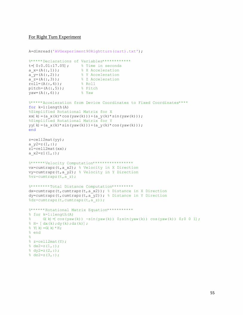
For Right Turn Experiment
A=dlmread('AVGexperiment90Rightturn(cart).txt');
%*****Declarations of Variables************ t=[0:0.01:17.05]; % Time in seconds a_x=(A(:,1)); % X Acceleration a_y=(A(:,2)); % Y Acceleration a_z=(A(:,3)); % Z Acceleration roll=(A(:,4)); % Roll pitch=(A(:,5)); % Pitch yaw=(A(:,6)); % Yaw
%*****Acceleration from Device Coordinates to Fixed Coordinates**** for k=1:length(A) %Simplified Rotational Matrix for X
xx{k}=(a_x(k)*cos(yaw(k)))+(a_y(k)*sin(yaw(k)));
%Simplified Rotational Matrix for Y
yy{k}=(a_x(k)*sin(yaw(k)))+(a_y(k)*cos(yaw(k))); end
z=cell2mat(yy); a_y2=z(1,:); z1=cell2mat(xx); a_x2=z1(1,:);
%******Velocity Computation***************** vx=cumtrapz(t,a_x2); % Velocity in X Direction vy=cumtrapz(t,a_y2); % Velocity in Y Direction %vz=cumtrapz(t,a_z);
%********Total Distance Computation********* dx=cumtrapz(t,cumtrapz(t,a_x2)); % Distance in X Direction dy=cumtrapz(t,cumtrapz(t,a_y2)); % Distance in Y Direction %dz=cumtrapz(t,cumtrapz(t,a_z));
%******Rotational Matrix Equation*********** % for k=1:length(A) % G{k}=[cos(yaw(k)) -sin(yaw(k)) 0;sin(yaw(k)) cos(yaw(k)) 0;0 0 1]; % H= [dx(k);dy(k);dz(k)]; % Y{k}=G{k}*H; % end % % z=cell2mat(Y); % dx2=z(1,:); % dy2=z(2,:); % dz2=z(3,:);
56
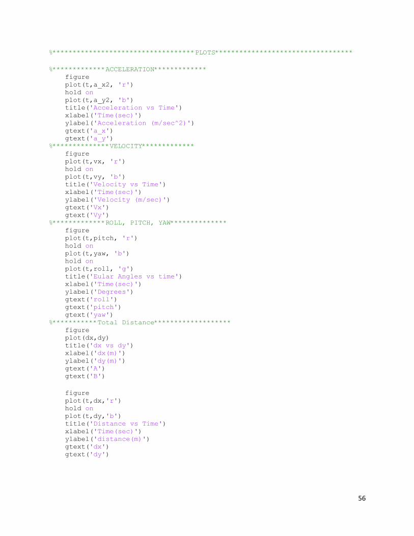
%***********************************PLOTS**********************************
%*************ACCELERATION************* figure plot(t,a_x2, 'r') hold on plot(t,a_y2, 'b') title('Acceleration vs Time') xlabel('Time(sec)') ylabel('Acceleration (m/sec^2)') gtext('a_x') gtext('a_y') %**************VELOCITY************* figure plot(t,vx, 'r') hold on plot(t,vy, 'b') title('Velocity vs Time') xlabel('Time(sec)') ylabel('Velocity (m/sec)') gtext('Vx') gtext('Vy') %*************ROLL, PITCH, YAW************** figure plot(t,pitch, 'r') hold on plot(t,yaw, 'b') hold on plot(t,roll, 'g') title('Eular Angles vs time') xlabel('Time(sec)') ylabel('Degrees') gtext('roll') gtext('pitch') gtext('yaw') %***********Total Distance******************* figure plot(dx,dy) title('dx vs dy') xlabel('dx(m)') ylabel('dy(m)') gtext('A') gtext('B')
figure plot(t,dx,'r') hold on plot(t,dy,'b') title('Distance vs Time') xlabel('Time(sec)') ylabel('distance(m)') gtext('dx') gtext('dy')