Int. J. Metrol. Qual. Eng. 4, 193–200 (2013)c© EDP Sciences 2014DOI: 10.1051/ijmqe/2013051

Performance study of dimensionality reduction methodsfor metrology of nonrigid mechanical parts

H. Radvar-Esfahlan� and S.-A. Tahan

Laboratoire d’Ingenierie des Produits, Procedes et Systemes (LIPPS), Ecole de Technologie Superieure, Montreal,H3C 1K3, Canada

Received: 29 June 2013 / Accepted: 20 October 2013

Abstract. The geometric measurement of parts using a coordinate measuring machine (CMM) has beengenerally adapted to the advanced automotive and aerospace industries. However, for the geometric inspec-tion of deformable free-form parts, special inspection fixtures, in combination with CMM’s and/or opticaldata acquisition devices (scanners), are used. As a result, the geometric inspection of flexible parts is aconsuming process in terms of time and money. The general procedure to eliminate the use of inspectionfixtures based on distance preserving nonlinear dimensionality reduction (NLDR) technique was developedin our previous works. We sought out geometric properties that are invariant to inelastic deformations.In this paper we will only present a systematic comparison of some well-known dimensionality reductiontechniques in order to evaluate their accuracy and potential for non-rigid metrology. We will demonstratethat even though these techniques may provide acceptable results through artificial data on certain fieldslike pattern recognition and machine learning, this performance cannot be extended to all real engineeringmetrology problems where high accuracy is needed.

Keywords: Computer aided inspection; geometric inspection; flexible parts; dimensionality reduction

1 Introduction

Geometric inspection, geometric modeling, range data ac-quisition and analysis have developed as separate fieldsof engineering among the various engineering and scien-tific communities. However, all these fields share commonscientific concepts, and there are many missed opportu-nities because of a lack of mutual connection and wastedsynergy. Computer-Aided Inspection is one of these con-nection points, while nonrigid geometric inspection sharesa profound degree of understanding of all the mentioneddisciplines. Currently, a flexible workpiece must be con-strained or clamped during the measurement process inorder to simulate the use state. To that end, expensiveand special inspection fixtures need to be designed andmanufactured [1]. On the other hand, some inspectionstages cannot be fully automated with this conventionalapproach. As a result, the geometric inspection of flexibleparts remains a time and money consuming process. Typi-cally some inspection set-up processes for nonrigid parts inaerospace industry request over 60 h of operations. On theother hand, even for simple parts, the quality of a plannedinspection depends on the ability and experience of the op-erator. Despite the multitude of papers and research thathave been produced in the CAD, CAM and CAI fields,

� Correspondence: hassan.radvar-esfahlan.1@ens.etsmtl.ca

the inspection of flexible parts continues to pose difficul-ties and significant costs to industries because they needspecial fixation devices. This is also evidence of the lackof knowledge and theoretical foundations surrounding thisspecial field. Our approach [2–4] was an effort to eliminatethe use of special inspection fixtures in the metrology offlexible parts. We tried to provide a better understand-ing of the developed algorithms by having the compar-ison between different existing methods. We also addedsome techniques to robustify our Generalized NumericalInspection Fixture (GNIF) [5]. Our philosophy was basedon the fact that the interpoint shortest path (geodesic dis-tance) between any two points on the parts remains un-changed during an isometric deformation. We called thisproperty distance preserving property of nonrigid parts. Infact GNIF was inspired by a real industrial inspection pro-cess. When a flexible part is put on an inspection fixturethe prevailing idea is that we are going to simulate thestate of use. But more specifically one can say that we arelooking for some correspondence between distorted partsand inspection fixtures, which represents our CAD-model.In spite of the accuracy of the presented methodology, thesimilarity detection process was extremely slow even forsimple parts with zero Gaussian curvature. In this paperwe will present a comparison of some well-known dimen-sionality reduction techniques in order to evaluate theiraccuracy and potential for non-rigid metrology.

Article published by EDP Sciences

194 International Journal of Metrology and Quality Engineering

In Section 2 a brief introduction to six NLDR meth-ods will be presented concisely with theirs mathematicalfundaments. Then in Section 3 described methods will beevaluated using some typical world engineering data. Theaim is to illustrate a systematic comparison and precisionfor each method.

2 Dimensionality reduction

Most problems in pattern recognition, such as image pro-cessing and speech recognition, begin with the preprocess-ing of high-dimensional signals. The complexity of mostlearning algorithms depends on the number of input di-mensions D. This is why we are interested in reducingthe embedding dimensionality with minimizing the loss ofinformation, of course in the literature there are two tech-niques for dimensionality reduction: feature selection andfeature extraction. In feature selection the aim is to find dof D dimensions (where d < D) which gives us the most in-formation. In other words we are interested in finding thebest subset of the set of the features. In metrology, featureselection is not a good approach for dimensionality reduc-tion because the individual vertices do not carry muchinformation on their own. It is the combination of verticesthat provides the most discriminative information. Thisis the idea behind the feature extraction techniques. Wetherefore consider the following problem. Given a high di-mensional data X = (x1, . . . , xn) where xi ∈ R

D the aimis to compute the output data Zi ∈ R

d that is the lowdimensional representation of X . For techniques used inthis paper only general information, including the steps foreach method, will be included without going into deriva-tion. Our focus in this paper is to compare the dimension-ality reduction methods on the geometric metrology viewpoint. Consequently, the aim is not to provide the detailsof the algorithms. We invite the reader to refer to theoriginal paper of each algorithm for further details. How-ever we will sketch a concise summary of each algorithmfor comparison and reference purposes. Next section dealswith methods that reduce the dimensionality of data byusing distance and topology preservation as the criterion.

2.1 Distance preserving DR techniques

For linear dimensionality reduction, some simple criterialike maximizing the variance preservation leads to one ofthe robust dimensionality reduction methods like Princi-pal Component Analysis (PCA) [6]. However in nonlinearcases the use of the same simple criteria requires morecomplex data models. On the other hand, every manifoldcan be described by its pairwise point distances whetherby Euclidean, graph or geodesics metrics. Tons of researchhas been undertaken and motivated by a simple fact: ifclose points are kept close and far points kept far, thenthe high dimensional data set and its low dimensional em-bedding share the same shape [7]. This section attemptsto review some of the best-known existing methods.

2.1.1 Multidimensional scaling (MDS)

Given the pairwise distance dij between n points andassuming that we don’t know the exact coordinates ofthe points and how the distance is calculated, MDS (alsoknown as Principal Coordinates Analysis [8]) tries to placethese points in low dimensional space in such a way thatthe Euclidean distance between them is as close as pos-sible to dij . Historically, the most significant achievementon MDS begins with Torgerson’s work in 1952 [9]. Be-fore then, Young and Householder [10] used the Euclideandistance as a metric of similarity measure. Let X and Ybe metric spaces and f : X → Y an arbitrary map. Thedistortion of f is defined by:

dis f = supa.b∈X

|dY (f(a), f(b)) − dX(a, b)| . (1)

The distance dX(a, b) between a pair of points in X ismapped to the distance dY (f(a), f(b)) between the imagesof a and b under f [11]. In our point cloud setting, wherethe shape X is sampled at N points X = {x1, . . . , xN},the distortion criteria will be:

σ = maxi,j=1,...,N

|dRm(f(xi), f(xj)) − dX(xi, xj)| . (2)

In MDS literature, the function σ which measures thedistortion of distances is called stress. Historically σ2 isused as the distortion criterion. Assume that Zi = f (xi)is a matrix of canonical form coordinates and dij(Z) =dRm(zi, zj), then:

σ2(Z; DX) =∑i>j

|dij(Z) − dX(xi, xj)|2. (3)

Here DX is a matrix of geodesic distances and dij(Z) isthe Euclidean distance between the points on the canon-ical form. The minimization algorithms which minimizethe stress function known as Multidimensional scaling.Historically MDS is classfied as a dimensionality reduc-tion method. Scaling by Majorizing a COmplicated Func-tion (SMACOF) is one of the well-known MDS algorithmsfor minimizing the stress function σ2(Z; DX) with respectto Z. This algorithm was proposed by De Leeuw [12].This algorithm is the core of our study in reference [4].Here we present a brief introduction on SMACOF. We re-fer the reader to [13] for an account. Before summarizingthe SMACOF algorithm, we describe some relations andnotations. Equation (3) can be written in matrix form:

σ2(Z; DX) = tr(ZT V Z) − 2tr(ZT B(Z; DX)Z)

+∑i>j

d2X(xi, xj). (4)

Here V is a constant N × N matrix with elements:

vij ={ −1 i �= j

N − 1 i = j(5)

H. Radvar-Esfahlan and S.-A. Tahan: Performance study of dimensionality reduction methods... 195

and B(Z; DX) is an N × N matrix with elements:

bij(Z; DX)=

⎧⎨⎩

−dX(xi, xj)d−1ij (Z) i �= j and dij(Z) �=0

0 i �= j and dij(Z)=0−∑

i�=k bik i = j.

(6)Thus, the SMACOF algorithm can be summarized as:

Algorithm 1: SMACOF algorithminput : matrix of geodesic distances

[DX ]N×N

output : canonical form Z∗1 set some initial Z(0) and k = 02 compute the raw stress σ2(Z(0); DX)3 repeat4 compute Z(k+1) = N−1B(Z(k); DX)Z(k)

(Guttman transform)5 compute the stress for this iteration,

σ2(Z(k+1); DX)6 compute the difference7 k = k + 18 until convergence9 set Z∗ = Z(k)

Step 6 of SMACOF algorithm contains findings for thedifference in the stress values between the two previousiterations. If it is less than some predefined tolerance orif the maximum number of iterations has been reached,then the algorithm stops.

2.1.2 Isometric feature mapping (ISOMAP)

This technique described by Tenenbaum et al. [14] is thevariant of MDS which uses graph distance (obtained byDijkstra algorithm [15]) as an estimation of geodesic dis-tance and applies MDS to lower the dimension of inputdata. The ISOMAP technique can be summerized as:

Algorithm 2: ISOMAP algorithm1 construct the graph of input data2 calculate the shortest pairwise distance between

all points3 apply the MDS to the shortest path found

in step 2

2.1.3 Maximum variance unfolding (MVU)

Weinberger and Saul [16] developed MVU algorithm (alsoknown as Semidefinite Embedding) based on mapping thehigh dimensional data set into a low dimensional spacethat preserves the distance and angle between nearby in-put patterns. In MDS the pairwise Euclidean distanceof input date sets was used as they were. In ISOMAP,Euclidean distance was replaced by geodesic distance. InMVU the transformation of distance is somehow more

complicated than in MDS and ISOMAP. Distances are as-sumed to be preserved locally, while nonlocal distances areoptimized in such a way that suitable embedding can befound. For instance, in 3D data sets the pairwise Euclideandistance is shorter than 2-dimensional embedding. There-fore MVU is considered to maximize the long distanceswhile maintaining the shortest ones.

To this end, the aim of the MVU is to unfold data bymaximizing pairwise distances, i.e.:

Max∑

ij‖�zi − �zj‖2 (7)

subject to

∀(i, j) ∈ edges; ... ‖�xi − �xj‖2 = ‖�zi − �zj‖2 (8)

and ∑i�zi = �0. (9)

The latter constraint was put in place to eliminate trans-lational degrees of freedom in the lower space by centeringthe output on the origin. The aforementioned optimizationobjective is a non-convex problem (multiple local minima)because it means maximizing a quadratic form subject toquadratic equality constraints. In reference [16] the au-thors propose a Semi definite Programming [17] techniqueby using dot products instead of squared distances. If Ddenotes the square matrix of squared Euclidean distances,and K the Gram matrices of X ; i.e. Kij = xi.xj , withoutgoing into detail, the MVU algorithm can be summarizedas follows:

Algorithm 3: MVU algorithm1 Compute all squared pairwise distances in matrix D

2 determine the k-nearest neighbours G,of each data point

3 find Maxtrace(K) subject to:kii + kjj − 2kij = ‖xi − xj‖2 for ∀(i, j) ∈ G∑

ij kij = 0K � 04 perform classical metric MDS on matrix K

2.1.4 Sammon’s mapping

The main weakness of MDS is that it tries to maintainlarge pairwise distances and does not retain the smallones [18]. Sammon’ Mapping (SM) [19] tries to overcomeMDS’ weakness by weighting the contribution of each pair.To this end, SM minimizes the following stress function:

ESM =1∑

ij dX(xi, xj)

∑i = 1i < j

(dX(xi, xj) − dZ(zi, zj))2

dX(xi, xj)

(10)where d is measured by Euclidean metrics. The minimiza-tion of Sammons’s stress function can be performed usinga pseudo-Newton optimization method.

196 International Journal of Metrology and Quality Engineering

2.1.5 Curvilinear component analysis (CCA)

Originally developed by Demartines and Herault [20],Curvilinear Component Analysis (CCA) is an improve-ment of Sammon’s mapping. This technique combinessome of the attitudes of SM and MDS along with artificialneural network strategies in order to map the higher di-mensional data to lower dimensional space. At first, CCAprocesses a vector quantization step [21] as a way to re-duce the data set size. Then like MDS, the authors defineda stress function in such a way as to preserve the inter-point distances during mapping. The CCA stress functionclosely resembles Sammon’s stress function:

ECCA =12

N∑i=1

N∑j=1

{dX(xi, xj) − dZ(zi, zj))2Fλ(dZ(zi, zj)

}

(11)

while we would like to have d(xi, xj) = d(zi, zj), this is notalways possible without distortion, so they introduced aweighting function Fλ. The choice of Fλ is based on thefact that preserving the short distances is more signifi-cant than the longer ones, because the long distances onthe manifold have to be stretched to unfold the manifold.Thus, Fλ was choosing as monotically decreasing func-tion [21]. In order to minimize cost function, Demartinesand Herault [20] developed a novel variant of gradient de-scent techniques. We refer the reader to their original workfor an account. In our study we didn’t sampled the rangedata. Therefore, the vector quantization is considered anoptional processing. Curvilinear Distance Analysis (CDA)developed by Lee et al. [22] is considered a variant of CCAwhich uses graph distance instead of Euclidean distance.

2.2 Topology preserving techniques

As depicted in the previous section dimensionality reduc-tion can be reached by distance preservation. In this cat-egory numerous methods were discussed. While the com-parative distances seem to give sufficient information onmanifold, most distance functions make no distinction be-tween manifold and its surrounding space. Topology pre-serving methods are another class of dimensionality reduc-tion techniques that tend to preserve important structuresof the data in the geometric structure of the mapping. Onesimple example of topology preserving maps is a Mercatorprojection of the earth into 2D space. While this kindof mapping gives invaluable visual information, distortioncan’t be prevented in some areas. In metrology, the topol-ogy gives the neighbourhood relationship between defectareas and the rest of the shape. The most problematicarea in topology preserving techniques is how to representa topology. All physical objects subjected to metrologyare continuous. Unfortunately continuous topology repre-sentation is not always possible. This is why discrete rep-resentation is used by a ‘lattice’ (or grid). In this categorywe have selected the most well-known technique which wewill summarize in the next section.

2.2.1 Locally linear embedding (LLE)

Locally linear embedding [23] is an eigenvector based tech-nique (like PCA and MDS) where optimization doesn’t in-volve local minima and iterative optimizations. It tries topreserve the local angles. LLE supposes that each pointwith its neighbors on the manifold lies on or close to alocally linear patch. Then it tries to characterize the lo-cal geometry of the patches by finding linear coefficientsthat reconstruct each point by using its k nearest neigh-bors. Roweis and Saul [23] measured the reconstructionerror by:

ε(w) =∑

i

∣∣∣xi −∑

jwijxj

∣∣∣2 (12)

where xj is the k-nearest neighbors of xi.wij summarizesthe contribution of the jth data point to the ith recon-struction and are found by optimizing equation (12) sub-ject to

∑j wij = 1. The authors found optimal weights by

using a least squares method. The final step of the algo-rithm is to reconstruct a representation zi of the xi in alow dimensional space. This was performed by minimizingthe embedding cost function:

Φ(z) =∑

i

∣∣∣zi −∑

jwijzj

∣∣∣2. (13)

The authors also proposed a sparse eigenvector problemin order to minimize the aforementioned cost function. Werefer the reader to LLE’s original paper for more detailson the minimization technique.

The comparison and review of DR methods on Patternclassification and Data visualization can be found inreferences [24, 25].

3 Experiment and results

In the previous section we summarized some well-knownNLDR techniques. In this section, the systematic compar-ison of the methods, along with their accuracy (minimumcorrespondence error) and performance in typical mechan-ical parts, will be investigated. To this end, we have cate-gorized the very real engineering problems to four groups.Flexible parts with:

(1) zero Gaussian curvature with sharp edge (studycase A);

(2) more complex shape with mostly zero Gaussiancurvature (study case B);

(3) free-form high curvature (study case C);(4) combination of both (study case D).

The aim of this study is to investigate the performanceof NLDR methods on nonrigid parts from the viewpointof metrology. To this end, all case studies (CAD-model &range data) are considered to be intrinsically similar [2].This means that all case studies considered are geomet-rically defectless. Figure 1 illustrates four case studiesinvestigated for this study. The models were created byCATIA� V5. Afterwards, a finite element analysis of the

H. Radvar-Esfahlan and S.-A. Tahan: Performance study of dimensionality reduction methods... 197

)B( )A(

)D( )C(

Fig. 1. Study cases.

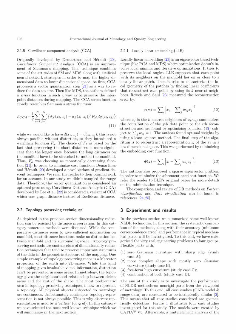
model was performed to simulate the free-state range data.At this point, a displacement and/or a force were appliedto the model to simulate spring back deformations. Thenarbitrary translational and rotational displacements wereadded to the range data. In this way, the CAD-model andrange data were simulated in different coordinate systems.Table 1 represents the geometric and mechanical proper-ties of the case studies. In order to compare similaritiesbetween the CAD-model and range data after reducingthe dimensionality, a Procrustes analysis was performed.Then the Euclidean distances between all correspondingpoints have been calculated. As an instance the perfor-mance study on the case study D is presented in Figure 2.All case studies were performed on an AMD Phenom(tm)II X4 B95 Processor 3.00 GHz PC using a 64-bit operat-ing system. Table 2 demonstrates the computational timefor each NLDR algorithm. The results of the analysis asmean (Accuracy) and standard deviation (Precision) forall study cases were illustrated in Table 3. The effect ofregistration error is considered to be equal for all casestudies.

Table 1. Geometric and mechanical properties of case studies.

Case Material Thickness Dimension # of nodesstudy [mm] [mm]

A Al-6061-T6 1.0 120 × 120 × 100 496B Al-6061-T6 2.0 100 × 100 × 80 701C Al-6061-T6 5.0 1600 × 1000 × 450 996D Al-6061-T6 0.5 340 × 130 × 50 1322

4 Discussion

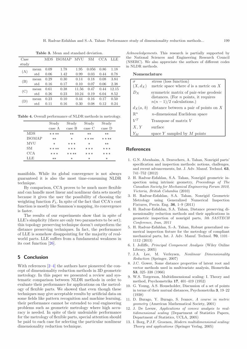
According to the results of means and standard devia-tions, Table 4 illustrates the overall performance of di-mensionality reduction methods for each study case. Forfree form high curvature parts (Study case C), a graphdistance based ISOMAP perform better than other meth-ods. This is something we already expected. In refer-ences [2–4] the authors used geodesics instead of graph dis-tance as a similarity measure. However experiments showsthat ISOMAP stands behind Sammon’s nonlinear map-ping as one of the computationally high casting methods.

198 International Journal of Metrology and Quality Engineering

(a) (b)

(c) (d)

(e) (f)

Fig. 2. 2D embedding of case study (D) using: (a) MDS; (b) ISOMAP; (c) MVU; (d) SM; (e) CCA; (f) LLE.

Classical MDS can be effectively used in simple partswith zero Gaussian curvature. On the other hand, classicalMDS stands to be the fastest among the others. The per-formance of ISOMAP is notably worse than classical MDSin cases where parts have zero Gaussian curvature withsharp corners. The reason behind this phenomenon is theerror of the geodesic/graph distance computation wherethe sharp bends occur. However, where the complexity in-creases (in the absence of sharp bends), ISOMAP offersmore chances to achieve good precision. Although MVUuses the graph distance, it doesn’t perform in the samemanner as ISOMAP. Classical scaling cost functions usedby Isomap retain the large geodesic/graph distances, whileMVU focuses on keeping the local/small structure data.

Table 2. Computational time [s].

Case MDS ISOMAP MVU SM CCA LLEstudy(A) 0.371 15.596 0.930 16.493 1.050 0.789(B) 0.782 33.202 3.073 40.840 2.236 1.097(C) 1.096 72.249 4.086 106.172 3.788 2.346(D) 1.912 140.833 6.004 297.410 5.345 4.525

MVU should be avoided in the case of free form highlycurved parts with large deformations where the curvaturechanges instantly.

Unlike classical MDS and MVU, Sammon’s mappingcan effectively handle all kinds of linear and nonlinear

H. Radvar-Esfahlan and S.-A. Tahan: Performance study of dimensionality reduction methods... 199

Table 3. Mean and standard deviation.

Case MDS ISOMAP MVU SM CCA LLE

study

(A)mean 0.09 1.78 1.95 0.056 0.86 1.18

std 0.06 1.42 0.99 0.03 0.44 0.78

(B)mean 0.29 0.30 0.14 0.18 0.08 3.84

std 0.16 0.17 0.10 0.07 0.06 2.38

(C)mean 0.61 0.38 11.56 0.47 0.44 12.15

std 0.26 0.23 10.24 0.19 6.04 8.52

(D)mean 0.23 0.10 0.44 0.16 0.17 0.50

std 0.11 0.16 0.30 0.08 0.12 0.24

Table 4. Overall performance of NLDR methods in metrology.

Study Study Study Study

case A case B case C case D

MDS � � �� �� �� ��

ISOMAP �� � � � �� � � ��

MVU � � � � � ��

SM � � �� � � � � � � � � �

CCA � � � � � �� � � � � � �

LLE �� � � �

manifolds. While its global convergence is not alwaysguaranteed it is also the most time-consuming NLDRtechnique.

By comparison, CCA proves to be much more flexibleand can handle most linear and nonlinear data sets mostlybecause it gives the user the possibility of choosing theweighting function Fλ. In spite of the fact that CCA’s costfunction is mostly like Sammon’s mapping, its convergenceis faster.

The results of our experiments show that in spite ofLLE’s simplicity (there are only two parameters to be set);this topology preserving technique doesn’t outperform thedistance preserving techniques. In fact, the performanceof LLE is somehow disappointing for the majority of real-world parts. LLE suffers from a fundamental weakness inits cost function [26].

5 Conclusion

With references [2–4] the authors have pioneered the con-cept of dimensionality reduction methods in 3D geometricmetrology. In this paper we presented a review and sys-tematic comparison between NLDR methods in order toevaluate their performance for applications on the metrol-ogy of flexible parts. We showed that even though thesetechniques may give acceptable results by artificial data onsome fields like pattern recognition and machine learning,their performance cannot be extended to real engineeringproblems such as geometric metrology where high accu-racy is needed. In spite of their undeniable performancefor the metrology of flexible parts, special attention shouldbe paid to each case for selecting the particular nonlineardimensionality reduction technique.

Acknowledgements. This research is partially supported bythe National Sciences and Engineering Research Council(NSERC). We also appreciate the authors of different codesin NLDR methods.

Nomenclature

σ stress (loss function)(X, dX) metric space where d is a metric on X

DX symmetric matrix of pair-wise geodesicdistances. (For n points, it requiresn(n − 1)/2 calculations.)

dX(a, b) distance between a pair of points on X

Rn n-dimensional Euclidean space

V T Transpose of matrix V

X , Y surface

YM space Y sampled by M points

References

1. G.N. Abenhaim, A. Desrochers, A. Tahan, Nonrigid parts’specification and inspection methods: notions, challenges,and recent advancements, Int. J. Adv. Manuf. Technol. 63,741–752 (2012)

2. H. Radvar-Esfahlan, S.A. Tahan, Nonrigid geometric in-spection using intrinsic geometry, Proceedings of TheCanadian Society for Mechanical Engineering Forum 2010,Victoria, British Columbia (2010)

3. H. Radvar-Esfahlan, S.A. Tahan, Nonrigid GeometricMetrology using Generalized Numerical InspectionFixtures, Precis. Eng. 36, 1–9 (2011)

4. H. Radvar-Esfahlan, S.A. Tahan, Distance preserving di-mensionality reduction methods and their applications ingeometric inspection of nonrigid parts, 5th SASTECHConference, Iran, 2011

5. H. Radvar-Esfahlan, S.-A. Tahan, Robust generalized nu-merical inspection fixture for the metrology of compliantmechanical parts, Int. J. Adv. Manuf. Technol. 70, 1101–1112 (2013)

6. I. Jolliffe, Principal Component Analysis (Wiley OnlineLibrary, 2005)

7. J.A. Lee, M. Verleysen, Nonlinear DimensionalityReduction (Springer, 2007)

8. J.C. Gower, Some distance properties of latent root andvector methods used in multivariate analysis, Biometrika53, 325–338 (1966)

9. W.S. Torgerson, Multidimensional scaling: I. Theory andmethod, Psychometrika 17, 401–419 (1952)

10. G. Young, A.S. Householder, Discussion of a set of pointsin terms of their mutual distances, Psychometrika 3, 19–22(1938)

11. D. Burago, Y. Burago, S. Ivanov, A course in metricgeometry (American Mathematical Society, 2001)

12. J. De Leeuw, Applications of convex analysis to mul-tidimensional scaling (Department of Statistics Papers,Department of Statistics, UCLA, 2005)

13. I. Borg, P.J.F. Groenen, Modern multidimensional scaling:Theory and applications (Springer Verlag, 2005)

200 International Journal of Metrology and Quality Engineering

14. J.B. Tenenbaum, V. De Silva, J.C. Langford, A global ge-ometric framework for nonlinear dimensionality reduction,Science 290, 2319–2323 (2000)

15. E. Dijkstra, A note on two problems in connexion withgraphs, Numer. Math. 1, 269–271 (1959)

16. K.Q. Weinberger, L.K. Saul, Unsupervised learningof image manifolds by semidefinite programming, inComputer Vision and Pattern Recognition, 2004. CVPR2004. Proceedings of the 2004 IEEE Computer SocietyConference on, 2004, Vol. 2, pp. II-988–II-995

17. L. Vandenberghe, S. Boyd, Semidefinite programming,SIAM Rev. 38, 49–95 (1996)

18. L. Van der Maaten, E. Postma, H. Van den Herik,Dimensionality reduction: A comparative review, J. Mach.Learn. Res. 10, 1–41 (2009)

19. J.W. Sammon Jr., A nonlinear mapping for data structureanalysis, Comput. IEEE Trans. 100, 401–409 (1969)

20. P. Demartines, J. Herault, Curvilinear component analy-sis: A self-organizing neural network for nonlinear mappingof data sets, Neural Netw. IEEE Trans. 8, 148–154 (1997)

21. A. Gersho, R.M. Gray, Vector Quantization and SignalCompression (Kluwer Academic Pub., 1992), Vol. 159

22. J.A. Lee, A. Lendasse, M. Verleysen, Curvilinear distanceanalysis versus isomap, in Proceedings of ESANN, 2002,pp. 185–192

23. S.T. Roweis, L.K. Saul, Nonlinear dimensionality reduc-tion by locally linear embedding, Science 290, 2323–2326(2000)

24. C.J. de Medeiros, J.A.F. Costa, L.A. Silva, A compar-ison of dimensionality reduction methods using topol-ogy preservation indexes, in Intelligent Data Engineeringand Automated Learning-IDEAL 2011 (Springer, 2011),pp. 437–445

25. H. Yin, Nonlinear dimensionality reduction and data visu-alization: a review, Int. J. Automat. Comput. 4, 294–303(2007)

26. J. Chen, Y. Liu, Locally linear embedding: a survey, Artif.Intell. Rev. 36, 29–48 (2011)