Performance report of the RHUM-RUM ocean bottom ... · 44 S. Stähler et al.: Performance report of the RHUM-RUM OBS network iment is a deployment of 48 German wideband and 9 French

Adv. Geosci., 41, 43–63, 2016

www.adv-geosci.net/41/43/2016/

doi:10.5194/adgeo-41-43-2016

© Author(s) 2016. CC Attribution 3.0 License.

Performance report of the RHUM-RUM ocean bottom seismometer

network around La Réunion, western Indian Ocean

S. C. Stähler1,6, K. Sigloch2,1, K. Hosseini1, W. C. Crawford3, G. Barruol4, M. C. Schmidt-Aursch5,

M. Tsekhmistrenko2,5, J.-R. Scholz4,5, A. Mazzullo3, and M. Deen3

1Dept. of Earth Sciences, Ludwig-Maximilians-Universität München, Theresienstrasse 41, 80333 Munich, Germany2Dept. of Earth Sciences, University of Oxford, South Parks Road, Oxford, OX1 3AN, UK3Institut de Physique du Globe de Paris, Sorbonne Paris Cité, UMR7154 – CNRS, Paris, France4Laboratoire GéoSciences Réunion, Université de La Réunion, Institut de Physique du Globe de Paris, Sorbonne Paris Cité,

UMR7154 – CNRS, Université Paris Diderot, Saint Denis CEDEX 9, France5Alfred Wegener Institute, Helmholtz Centre for Polar and Marine Research, Am Alten Hafen 26,

27568 Bremerhaven, Germany6Leibniz-Institute for Baltic Sea Research, Seestraße 15, 18119 Rostock, Germany

Correspondence to: S. Stähler ([email protected])

Received: 21 July 2015 – Revised: 23 December 2015 – Accepted: 21 January 2016 – Published: 2 February 2016

Abstract. RHUM-RUM is a German-French seismological

experiment based on the sea floor surrounding the island of

La Réunion, western Indian Ocean (Barruol and Sigloch,

2013). Its primary objective is to clarify the presence or

absence of a mantle plume beneath the Reunion volcanic

hotspot. RHUM-RUM’s central component is a 13-month

deployment (October 2012 to November 2013) of 57 broad-

band ocean bottom seismometers (OBS) and hydrophones

over an area of 2000× 2000 km2 surrounding the hotspot.

The array contained 48 wideband OBS from the German DE-

PAS pool and 9 broadband OBS from the French INSU pool.

It is the largest deployment of DEPAS and INSU OBS so far,

and the first joint experiment.

This article reviews network performance and data qual-

ity: of the 57 stations, 46 and 53 yielded good seismome-

ter and hydrophone recordings, respectively. The 19 751 total

deployment days yielded 18 735 days of hydrophone record-

ings and 15 941 days of seismometer recordings, which are

94 and 80 % of the theoretically possible yields.

The INSU seismic sensors stand away from their OBS

frames, whereas the DEPAS sensors are integrated into their

frames. At long periods (> 10 s), the DEPAS seismome-

ters are affected by significantly stronger noise than the

INSU seismometers. On the horizontal components, this can

be explained by tilting of the frame and buoy assemblage,

e.g. through the action of ocean-bottom currents, but in ad-

dition the DEPAS intruments are affected by significant self-

noise at long periods, including on the vertical channels. By

comparison, the INSU instruments are much quieter at pe-

riods > 30 s and hence better suited for long-period signals

studies.

The trade-off of the instrument design is that the inte-

grated DEPAS setup is easier to deploy and recover, espe-

cially when large numbers of stations are involved. Addi-

tionally, the wideband sensor has only half the power con-

sumption of the broadband INSU seismometers. For the first

time, this article publishes response information of the DE-

PAS instruments, which is necessary for any project where

true ground displacement is of interest. The data will become

publicly available at the end of 2017.

1 Introduction

RHUM-RUM, short for “Reunion Hotspot and Upper Mantle

– Réunions Unterer Mantel”, is a German-French experiment

that investigates the mantle beneath the Reunion ocean island

hotspot from crust to core, using a multitude of seismologi-

cal and marine geophysical methods (Barruol and Sigloch,

2013). The project also studies the hypothesized interaction

between the hotspot and its surrounding mid-ocean ridges

(Morgan, 1978; Dyment et al., 2007). The core of the exper-

Published by Copernicus Publications on behalf of the European Geosciences Union.

44 S. Stähler et al.: Performance report of the RHUM-RUM OBS network

iment is a deployment of 48 German wideband and 9 French

broadband ocean-bottom seismometers (OBS), from the DE-

PAS (Deutscher Geräte-Pool für Amphibische Seismologie,

managed by AWI Bremerhaven) and INSU (Institut national

des sciences de l’Univers) pools respectively (see Table 1 for

the data return).

There have been multiple experiments in tectonic settings

similar to RHUM-RUM: 35 wideband and broadband OBS

from the US OBS Instrument Pool (OBSIP) were deployed

by the PLUME Hawaii experiment (Laske et al., 2009; Wolfe

et al., 2009) twice for 1 year. Japanese large-scale imaging

efforts around an oceanic hotspot were the PLUME Tahiti

experiment with 9 Japanese broadband OBS (BBOBS) (Bar-

ruol, 2002; Suetsugu et al., 2005) and the TIARES array

with again 9 BBOBS around the Society hotspot (Suetsugu

et al., 2012). In 2011–2012, 24 German DEPAS OBS were

deployed around the Tristan da Cunha hotspot (ISOLDE ex-

periment, Geissler and Schmidt, 2013). Other larger, long-

term DEPAS deployments in non-hotspot settings were in

the Aegean Sea (EGELADOS, Meier et al., 2007) and in the

Gulf of Cadiz (NEAREST, Geissler et al., 2010).

RHUM-RUM has been the largest DEPAS deployment so

far in terms of the number of stations deployed (44+ 4) and

in terms of aperture. This allows to resolve the deep-mantle

signature of a plume using seismic tomography, especially

when combined with concurrent land deployments. It is the

first OBS experiment that specifically tries to use data for

waveform tomography. This requires full response informa-

tion on all instruments and also a high signal-to-noise ratio

in the whole frequency range between 0.01 and 1 Hz.

The central component of the experiment was a deploy-

ment of 44 wideband OBS from DEPAS, of the so-called

“LOBSTER” (Longterm OBS for Tsunami and Earthquake

Research) type; 4 from Geomar Kiel, essentially identical to

the DEPAS LOBSTERs; and 9 LCPO2000 broadband OBS

from INSU, which are based on the “L-CHEAPO” instru-

ment (Low-Cost Hardware for Earth Applications and Phys-

ical Oceanography) developed at the Scripps Institution of

Oceanography (SIO).

We report on, and compare, the performance of seis-

mometers and hydrophones from the two involved instru-

ment pools, the German DEPAS and the French Parc Sis-

momètre Fond de Mer of INSU. This is the first side-by-

side comparison of instruments from the German and French

community OBS pools.

Data from the RHUM-RUM ocean bottom stations (and

island stations) will be made freely available at the end of

2017 (Barruol et al., 2011).

This paper reviews the functioning of the OBS network

and documents issues encountered in data collection, quality

control, and processing. We review the experiment layout in

Sect. 2.1, and the two types of OBS employed in Sect. 2.2.

The performance of the stations is described in Sect. 3, with

a focus on noise levels in Sect. 3.3. Possible reasons for the

surprisingly different noise levels are discussed in Sect. 4.

Table 1. Data return in RHUM-RUM experiment.

Data return: # of stations

Data return on all four channels throughout

the entire deployment:

27

Data return on all four channels for only

part of the deployment:

18

Only hydrophone data throughout the entire

deployment:

1

Only hydrophone data for only part of the

deployment:

7

No data returned: 4

Total number of stations deployed: 57

Data days recorded:

Data days (hydrophones): 18 735

Data days (seismometers): 15 941

Deployment days: 19 751

Percent data recovery (hydrophones): 94 %

Percent data recovery (seismometers): 80 %

Appendix A contains a detailed description of the seismome-

ter instrument responses, Appendix B describes an experi-

ment to estimate clock drift rates and Appendix C contains a

station-by-station list of noise levels in three period bands.

2 Experiment setup and instrumentation

2.1 The OBS network

For an overview of the whole network see Fig. 1. The oceanic

component of the RHUM-RUM experiment consisted of

57 broadband ocean bottom seismometers deployed over an

area of 2000 km× 2000 km from September 2012 to Novem-

ber 2013. The OBS clustered relatively densely around the

island of La Réunion, out to distances of 400–500 km, in-

cluding the vicinity of Mauritius (Fig. 1). This relative dense

coverage was extended eastward to the Central Indian Ridge,

in order to investigate hypothesized asthenospheric flow from

hotspot to ridge (Morgan, 1978; Dyment et al., 2007). The

seismicity in the reliably active South Sandwich subduction

zone generates body-wave paths which sample the mantle

beneath La Réunion at greater depths. Sampling with op-

posite azimuth is provided by earthquakes in the subduction

zones of the south west Pacific, especially since the OBS net-

work is augmented by RHUM-RUM land stations on Mada-

gascar, and on the Îles Éparses in the Mozambique Channel.

A linear, less dense arrangement of OBS followed the strike

of the Central Indian and Southwest Indian ridges to the east

and south, at 800–1200 km distance from the hotspot. Waves

originating from earthquakes in the Alpine-Himalayan oro-

gens and recorded at these stations again sample deeper lev-

els of the mantle beneath La Réunion, but are also used to

study the mid-ocean ridges themselves. A dense sub-array

Adv. Geosci., 41, 43–63, 2016 www.adv-geosci.net/41/43/2016/

S. Stähler et al.: Performance report of the RHUM-RUM OBS network 45

35°S

30°S

25°S

20°S

15°S

45°E 50°E 55°E 60°E 65°E 70°E

0 300 600

km

RR01RR02

RR03

RR04RR05

RR06RR07

RR08

RR09RR10

RR11RR12RR13RR14RR15

RR16

RR17RR18RR19

RR20

RR21RR22

RR23

RR24

RR25RR26

RR27

RR28

RR29

RR30

RR31

RR32

RR33

RR34

RR35

RR36

RR37

RR38

RR39

RR40

RR49

RR50

RR51

RR52RR53

RR55RR56

RR57

RUM1RUM2

RUM3RUM4

RUM5

TROM

RR01

RR03

RR05

RR06RR07

RR08

RR09RR10

RR11RR12RR13RR14

RR16

RR17RR18RR19

RR20

RR21RR22

RR23

RR24

RR25RR26

RR27

RR28

RR29

RR30

RR31

RR32

RR33

RR34

RR35

RR36

RR37

RR38

RR39

RR40

RR49

RR50

RR51

RR52RR53RR54RR55

RR56

RR57

RUM1RUM2

RUM3RUM4

RUM5

TROM

Hydrophone fine

Hydrophone noisy

Hydrophone failed

Seismometer fine

Seismometer noisy

Seismometer failed

DEPAS OBS

INSU OBS

Geomar OBS

120s instrument

RR land station

Temporary land station

Permanent land station

Depth

-6000 m

-5000 m

-4000 m

-3000 m

-2000 m

-1500 m

-1000 m

-500 m

-200 m

-100 m

0 m

SWIR array

RR41

RR42RR44

RR45

RR46

RR47

RR48

RR41

RR42RR43 RR44

RR45

RR46

RR47

RR48

50 km

La Reunion

RERRER

50 km

Figure 1. Overview map of the RHUM-RUM ocean bottom seismometer network. OBS are marked by large coloured symbols. Symbol

shape marks the station type: DEPAS LOBSTER (inverted triangle), INSU LCPO2000 (circle), Geomar OBS (star). DEPAS instruments

with malfunctioning 120 s instruments are marked as regular triangles. Two halves of the inner symbol indicate the functioning of the

seismic sensors and hydrophones, respectively. Green indicates good performance; orange, high noise levels; red means the instrument failed

to record. White squares indicate temporary land stations as part of the RHUM-RUM network YV, grey square indicate temporary land

stations as part of the MACOMO (Wysession et al., 2012) and SELASOMA (Tilmann et al., 2012) projects, which were both installed

between 2012 and 2014. Black squares indicate permanent GEOSCOPE stations. Small black dots mark earthquake hypocentres above

magnitude 4 between 1981 and 2015, as published by the Preliminary Determination of Epicentres (PDE) bulletin of the US National

Earthquake Information Center (NEIC). The seismicity is mainly concentrated on the oceanic ridges. Colour-shaded bathymetry is based on

the global 30 arcsec merged bathymetry dataset by Becker et al. (2009), available at: http://topex.ucsd.edu/WWW_html/srtm30_plus.html.

of 8 OBS, referred to as the “SWIR Array”, was deployed

around an active seamount on the Southwest Indian Ridge in

order to investigate the structure and seismicity of this ultra-

slow spreading ridge. The sub-array had a footprint of about

70 km× 50 km and was located in segment 8 of the ridge,

following the nomenclature of Cannat et al. (1999).

The OBS were deployed in October 2012 by the French re-

search vessel Marion Dufresne and were recovered in Octo-

ber/November 2013 by the German research vessel Meteor.

The instruments spent the intervening 13 months recording

on the seafloor.

At each deployment site, the seafloor was surveyed with

R/V Marion Dufresne’s multi-beam bathymeter and sedi-

ment echo sounder before dropping the OBS over board in

a location deemed most suitable. The ship left immediately

after deployment so that only deployment (and recovery) co-

ordinates are known; no attempt was made to acoustically tri-

angulate the landing positions of the OBS, with the notable

exception of the 8 OBS in the densified SWIR Array. In gen-

eral, OBS recovery positions were found to differ from their

deployment positions by no more than a few hundred meters.

2.2 OBS models deployed

Here we give a brief overview of the hardware deployed (see

Table 2) and the recording settings used, especially as they

relate to the performance assessment of Sect. 3 (see Table 2

for an overview).

2.2.1 LOBSTER

The broadband OBS pool DEPAS (Deutscher Geräte-Pool

für Amphibische Seismologie) of the German geophysical

community consists of 80 instruments of the LOBSTER type

(“Long-term OBS for Tsunami and Earthquake Research”).

The OBS were developed in 2005, merging previous de-

sign experience mainly by Geomar Kiel (Flueh and Biolas,

1996), the University of Hamburg (Dahm et al., 2002), and

the marine engineering firm K.U.M. (Umwelt- und Meer-

estechnik Kiel). K.U.M. was charged with building 80 LOB-

STER units, which were funded by the German Research

Foundation (DFG), the Federal Ministry of Education and

Research (BMBF) and the Helmholtz Association of Na-

tional Research Centres (HGF). The Alfred Wegener Insti-

tute Bremerhaven houses and maintains the instruments. For

www.adv-geosci.net/41/43/2016/ Adv. Geosci., 41, 43–63, 2016

http://topex.ucsd.edu/WWW_html/srtm30_plus.html


Figure 2. Broadband ocean-bottom seismometers, photographed seconds before deployment. Left panel: one of 48 LOBSTER-type instru-

ments from the German DEPAS pool. The Güralp CMG-OBS40T sensor (corner period 60 s) is fitted in a vertical titanium pressure cylinder

between two syntactic foam buoys and wedged against the steel anchor beneath it. Two horizontal titanium cylinders in the background

contain the data recorder and the lithium batteries. The broadband hydrophone (corner period 100 s) is strapped to the A-shaped titanium

frame that protrudes from the centre of the buoy assemblage. Right panel: one of 9 LCPO2000-BBOBS (Scripps-based) instruments from

the French Parc de Sismomètre Fond de Mer pool at INSU. The Nanometrics Trillium sensor (corner period 240 s) is contained in the green

sphere, which is dropped (i.e. mechanically separated) from the main frame one hour after arrival on the seabed. The differential pressure

gauge is located in the white cylinder behind the frame. Both instruments are equipped with flags, strobe lights and radio beacons to facilitate

recovery.

detailed information see http://www.awi.de/depas. The four

OBS loaned to RHUM-RUM by Geomar Kiel are essentially

identical to the DEPAS OBS.

The modular LOBSTER design (Fig. 2, left panel) is based

on an open titanium frame that holds three titanium cylin-

ders (containing the seismic sensor, data acquisition unit,

and lithium batteries) and syntactic foam buoys that provide

buoyancy for the ascent during recovery. A fourth titanium

cylinder contains a mechanical release unit that locks the

frame assemblage to a steel anchor until an acoustic release

signal is received that initiates detachment from the anchor.

The hydrophone is strapped to the frame, as are various re-

covery aides (a radio beacon, a flash, a flag, and a head buoy).

The titanium tube holding the seismic sensor is seated

vertically between two syntactic foam units, and is wedged

against the steel anchor by a steel plate, which acts as a lever

that is pre-loaded by the mechanical release unit, thus ensur-

ing good seismic coupling to the anchor. The integration of

the seismometer into the frame makes the design very sturdy

and reduces the number of failure points, but it also means

that the seismometer is likely to record any tilt noise created

by currents or pressure fluctuations acting on the frame. The

orientation of the seismometer channels is fixed with respect

to the frame, as it is shown in Fig. 3.

The seismic sensor in most DEPAS units is a three-

component wideband Güralp CMG-OBS40T with a corner

period of 60 s. The CMG-OBS40T is a lesser-known version

of the CMG-40T with reduced power consumption, which

is mounted in a gimbal system for usage in OBS. The gim-

bal system is activated three days after arrival on the seafloor

to ensure proper levelling, since the instrument may land in a

X/1

Seismometer

Y/2

Figure 3. Sketch of a LOBSTER frame with the orientation of the

horizontal seismometer channels. The X channel is oriented along

the long axis of the LOBSTER, the Y channel 90◦ clock-wise of it.

Positive values in the seismogram correspond to movement in the

direction of the arrow. For the vertical (Z) channel, positive values

correspond to upward movement. In the RESIF data archive, the

X channel is stored as BH1, the Y channel as BH2 and the Z chan-

nel as BHZ.

tilted position) and then once every 21 days since the seafloor

may settle over time.

The seismometer is sold in versions with different upper

corner periods (10, 30, 60 s). All are mechanically identical,

but use different feedback mechanisms to control the flat part

of the response curve. The 60 s version is used by DEPAS

and other OBS pools in Europe (e.g. IDL, Lisbon). Nine out

of 48 instruments used in RHUM-RUM featured a prototype,

broadband sensor design (corner period of 120 s). All of these

nine units failed to level under deep-sea conditions, and re-

peated, unsuccessful levelling attempts drained the batteries

prematurely (see Sect. 3.1).

The DEPAS units were additionally equipped with broad-

band hydrophones of type HTI-01 and HTI-04-PCA/ULF


http://www.awi.de/depas


Table 2. Comparison of German (DEPAS) and French (INSU-

IPGP) OBS types.

Pool DEPAS INSU-IPGP

Manufacturer K.U.M., Kiel Scripps/INSU-

IPGP

OBS type LOBSTER LCPO2000-

BBOBS

Weight (water/air) 30/400 kg 25/350 kg

Assembly time 30 min (2 persons) 2 h (2 persons)

Transport options 12 in a 20′ container 8 in a 20′ container

Buoyancy Syntactic foam Glass spheres

Instrument casing Titanium Aluminium

Seismometer CMG-OBS40T

(60/120 s)

Trillium 240OBS

(240 s)

Placement integrated into frame in external probe

Power consumption 100 mW (seism.) 700 mW (seism.)

520 mW (recorder) 600 mW (recorder)

manufactured by HighTechInc (corner period 100 s), which

usually worked very reliably as long as power was available.

The deepest RHUM-RUM OBS was deployed at 5400 m

depth (Table 3), and the standard DEPAS OBS is certified to

6000 m water depth. Two battery tubes can be fitted with up

to 180 lithium cells, sufficient for up to 15 months of record-

ing using the settings described below. RHUM-RUM instru-

ments were equipped to record for 13 months at sampling

rates of 50 Hz. Eight of the 48 available DEPAS units were

of a deep-diving variant certified to 7300 m depth, which

has only one battery tube and therefore holds fewer batter-

ies. Most of these instruments were deployed in the SWIR

sub-array and typically recorded for 8–9 months at a sam-

pling rate of 100 Hz (higher rate in order to investigate lo-

cal seismicity). The clocks are supposed to continue running

even after the voltage has dropped below the level required

for data recording, in order to enable estimates of clock drift

even if OBS retrieval is delayed.

2.2.2 The Scripps OBS instrument, INSU instrument

pool

The INSU instruments (Fig. 2, right panel) are of the

LCPO2000-BBOBS type, which is based on the Scripps

Institution of Oceanography (SIO) “L-CHEAPO” design.

Three of the instruments were manufactured at SIO and the

other six at the INSU-IPGP OBS facility. The data recorder,

batteries and release unit are protected in aluminium cylin-

ders. The seismic sensor sits in an aluminium sphere. Buoy-

ancy for recovery is created by hollow glass spheres.

All instruments were equipped with Nanometrics

Trillium-240 seismometers with a corner period of 240 s

and a differential pressure gauge with a passband between

0.002 to 30 Hz.

The INSU instruments check their level every hour. This

caused an electronic spike of approximately 600 counts on

the seismometer channels (see Sect. 3). This same spike ex-

ists in the 2006–2007 PLUME data set using SIO BBOBS

(Laske et al., 2009), although we found no published men-

tion of it. The problem has not been explicitly solved, but the

SIO BBOBSs were reprogrammed after the PLUME experi-

ment to only check level once a week after the initial level-

ling cycle and the INSU BBOBSs are currently being repro-

grammed to do the same. Work has been done to remove the

hourly spike in the PLUME data (G. Laske, personal commu-

nication, 2014) and is being repeated for the RHUM-RUM

data: it would be good to publish the correction algorithms,

because these instruments probably still have this spike once

per week.

The INSU instruments use a differential pressure gauge

(DPGs, Cox et al., 1984) rather than a hydrophone. The DPG

sits on the lower instrument frame close to the battery cylin-

der (Fig. 2).

2.3 Instrument responses

Instrument responses specify the transfer functions of seis-

mometers and hydrophones (three seismogram channels and

one hydrophone channel per station). The RESIF (RÉseau

SIsmologique & géodésique Français) data centre serves this

information in the format of StationXML or dataless SEED

files.

To our knowledge, detailed meta-data information for DE-

PAS OBS has not been published elsewhere. Therefore, we

added a detailed discussion of the instrument responses as

an appendix to this paper (Sect. A). Figures 4 and 5 show

the total responses of instruments and data loggers for hy-

drophones and seismometers. Figure 6 shows instrument-

corrected waveforms. For all seismometer types, instrument

correction results in the same P-waveform.

3 Network performance

All 57 OBS were recovered successfully and undamaged.

Table 3 summarizes the state of health of all seismometers

and hydrophones over the deployment period. For a graphi-

cal summary of network performance (see Fig. 7).

Deployments were staggered over four weeks, along the

15 000 km-long cruise track. Recovery took five weeks and

proceeded in roughly the same order as deployment, so that

all stations spent approximately 13 months on the sea floor.

An early end of recording was anticipated for stations RR35,

RR41, RR43–RR48, and RR51 because their single battery

tube only accommodated batteries for 8–9 months. For other

stations, premature end of recording reflects technical issues,

as discussed below.

Following the definition of the Cascadia initiative (Sumy

et al., 2015), the data recovery was 15 941 data days out of

19 751 deployment days or 80 % for the seismometers, and

18 735 data days or 94 % for the hydrophones (Table 1).



Table 3. Performance summary of the 57 RHUM-RUM OBS and hydrophones. The abbrevation “gz” in the status column refers to the

“glitch” on the Z component of the INSU seismograms (see Sect. 3.1). Skew is the measured clock drift in s, i.e. the instrument time at

recovery minus the GPS time at recovery (“NA” if unknown because clock stopped early). For DEPAS stations, the number of recording

days can exceed the number of deployment days because recording was started on deck prior to deployment. In the comments column,

“120 s inst.” refers to the new DEPAS sensor type that failed to level, yielding no useful seismometer data; “Geomar” refers to an OBS from

Geomar, similar to the DEPAS LOBSTER. Figure 7 summarizes the network’s state of health over the deployment period of October 2012

to November 2013.

Station

name

Latitude Longitude Depth

[m]

Deployment

date

[UTC]

Recovery

date

[UTC]

End of

record

[UTC]

Install. time

[days]

Record

length

[days]

s.r. [Hz] Seismo

status

Hydro

status

Skew

value

Notes

RR01 −20.0069 55.4230 4298 5 Oct 2012 6 Nov 2013 6 Nov 2013 397 397 50 good good 0.67 s

RR02 −20.3392 54.4984 4436 5 Oct 2012 6 Nov 2013 5 Oct 2012 396 0 50 failed failed NA


RR04 −22.2553 55.3846 4168 5 Oct 2012 5 Nov 2013 7 Oct 2012 396 2 50 failed failed NA


RR06 −20.6550 56.7639 4216 3 Oct 2012 7 Nov 2013 31 Oct 2013 399 393 50 good good NA

RR07 −20.1945 59.4058 4370 29 Sep 2012 24 Oct 2013 24 Oct 2013 389 389 50 good good 0.53 s




RR11 −18.7784 65.4629 3941 1 Oct 2012 26 Oct 2013 26 Oct 2013 390 390 50 good good 0.61 s

RR12 −18.9255 63.6474 3185 1 Oct 2012 26 Oct 2013 26 Oct 2013 390 390 50 good good −0.11 s

RR13 −18.5427 60.5635 4130 2 Oct 2012 27 Oct 2013 9 Oct 2013 390 372 50 good good NA


RR15 −17.7402 58.3330 3959 2 Oct 2012 28 Oct 2013 4 Oct 2012 390 1 50 failed failed NA








RR23 −22.3290 50.4487 4893 10 Oct 2012 31 Oct 2013 26 Aug 2013 386 320 50 failed good NA 120 s inst

RR24 −25.6805 54.4881 5074 22 Oct 2012 3 Nov 2013 8 Oct 2013 376 291 50 failed good NA 120 s inst



RR27 −21.9657 54.2889 4277 5 Oct 2012 5 Nov 2013 19 Jul 2013 396 286 50 noisy good NA

RR28 −22.7152 53.1595 4540 10 Oct 2012 12 Nov 2013 12 Nov 2013 398 397 62.5 good (gZ) good 3.10 s INSU


RR30 −26.4861 49.8917 5140 11 Oct 2012 14 Nov 2013 8 Oct 2013 398 361 50 good good NA

RR31 −28.7648 48.1394 2710 12 Oct 2012 15 Nov 2013 15 Nov 2013 398 398 62.5 good (gZ) noisy −0.83 s INSU

RR32 −30.2903 49.5555 4670 12 Oct 2012 15 Nov 2013 6 Nov 2013 398 358 50 failed good NA 120 s inst

RR33 −31.1170 50.6835 4904 13 Oct 2012 16 Nov 2013 19 Sep 2013 399 341 50 noisy noisy NA Geomar

RR34 −32.0783 52.2113 4260 13 Oct 2012 16 Nov 2013 16 Nov 2013 399 398 62.5 good (gZ) good −1.29 s INSU

RR35 −32.9694 54.1473 4214 13 Oct 2012 17 Nov 2013 27 May 2013 399 225 50 failed noisy NA 120 s inst


RR37 −31.7010 57.8876 4036 14 Oct 2012 18 Nov 2013 19 Oct 2013 399 369 50 noisy good NA

RR38 −30.5650 59.6858 4540 15 Oct 2012 19 Nov 2013 19 Nov 2013 399 399 62.5 good (gZ) good −0.06 s INSU

RR39 −29.0165 60.9755 4700 15 Oct 2012 19 Nov 2013 19 Nov 2013 400 400 50 failed noisy NA Geomar


RR41 −27.7330 65.3344 5430 16 Oct 2012 20 Nov 2013 17 Jun 2013 400 244 100 good good NA

RR42 −27.6192 65.4376 4776 16 Oct 2012 21 Nov 2013 10 Aug 2013 400 298 50 failed good NA 120 s inst



RR45 −27.6581 65.6019 2822 16 Oct 2012 21 Nov 2013 4 Jun 2013 400 138 100 noisy good NA



Table 3. Continued.

Station

name

Latitude Longitude Depth

[m]

Deployment

date

[UTC]

Recovery

date

[UTC]

End of

record

[UTC]

Install. time

[days]

Record

length

[days]

s.r. [Hz] Seismo

status

Hydro

status

Skew

value

Notes

RR46 −27.7909 65.5835 3640 16 Oct 2012 21 Nov 2013 26 May 2013 400 221 100 good good NA



RR49 −26.2742 68.5354 4444 17 Oct 2012 23 Nov 2013 6 Nov 2013 401 384 50 failed good NA 120 s inst


RR51 −22.9989 69.1911 3463 18 Oct 2012 24 Nov 2013 3 Jan 2013 401 76 50 failed failed NA 120 s inst


RR53 −20.1213 64.9664 2940 20 Oct 2012 28 Nov 2013 30 Oct 2013 403 375 50 good good NA Geomar

RR54 −20.6424 63.5082 2499 20 Oct 2012 28 Nov 2013 21 Oct 2013 404 365 50 failed good NA 120 s inst

RR55 −21.4417 61.4959 4462 20 Oct 2012 28 Nov 2013 8 Nov 2013 404 383 50 good good NA

RR56 −21.9694 59.5853 4230 21 Oct 2012 29 Nov 2013 29 Jun 2013 404 251 50 good good NA Geomar

RR57 −24.7264 58.0496 5200 21 Oct 2012 3 Nov 2013 31 Oct 2013 378 374 50 failed good 1.28 s 120 s inst

10-3 10-2 10-1 100 101 102106

107

108

109

1010

Am

plit

ude /

(co

unts

/(m

/s))

1

7.0e+08

1

7.4e+08

INSU BHZ DEPAS BHZ

10-3 10-2 10-1 100 101 102

Frequency / Hz

/2

0

- /2

Phase

Figure 4. Bode plot of the total instrument responses G(f ) as de-

fined in Eq. (A2) of vertical seismometer components, for a DEPAS

Güralp CMG-OBS40T seismometer (solid green, station RR26),

and for an INSU Trillium-240 (dashed blue, RR28). The corner pe-

riod is 60 s for DEPAS instruments and 240 s for INSU instruments,

which is evident from the amplitude responses. Horizontal channel

responses of DEPAS instruments are identical to vertical responses,

apart from the channel-specific gain, which varies by a few percent.

The horizontal gain of INSU sensors is 1.6× 108 counts(m s1)−1

compared to of 7.0× 108 counts(m s1)−1 for the vertical channel.

The upper frequency limits (dotted lines) are given by the Nyquist

frequencies (1/2× 50 Hz for RR26 and 1/2× 62.5 Hz for RR28).

3.1 Instrument failures

Three out of 48 DEPAS stations (RR02, RR04, RR15) de-

livered neither seismometer nor hydrophone data because

their data loggers failed (reason unclear). The seismometers

in nine DEPAS stations (RR23, RR24, RR32, RR35, RR42,

RR49, RR51, RR54, RR57) featured a redesigned sen-

10-3 10-2 10-1 100 101 102100

101

102

103

104

Am

plit

ude /

(co

unts

/Pa)

1

5.0e+02

1

1.8e+03

INSU BDH DEPAS BDH

10-3 10-2 10-1 100 101 102

Frequency / Hz

-

- /2

0

/2

Phase

Figure 5. Bode plot of the total instrument responses G(f ) as de-

fined in Eq. (A2) of a DEPAS HighTechInc HTI-PCA04/ULF hy-

drophone (solid green, station RR26), and of an INSU differential

pressure gauge (dashed blue, RR28). The nominal corner period is

100 s for DEPAS instruments and 500 s for INSU instruments. Dot-

ted lines mark the Nyquist frequencies (see above).

sor/casing package with broader band CMG-OBS40T sen-

sors (120 s), which had previously not been deployed in the

deep sea. The levelling mechanisms failed (remained stuck)

in all nine stations, for reasons that are still under investi-

gation. Automatic, prolonged attempts to level the sensors

drained their batteries prematurely so that the functioning

hydrophones also ran out of power 8–9 months into the ex-

periment. DEPAS seismometers RR27 and RR45 recorded,

but at high noise levels (reason under investigation). The hy-

drophones of these stations worked normally. The seismome-

ter in one of the four Geomar stations failed (RR39), and

noise levels at Geomar station RR33 are unusually high, al-



−50 0 50 100 150 200

RR52

RR10

TROM

RR05

RR19

RR20

RR25

RR40

RR03

RR34

Time (sec)Time (sec)

RR52

RR10

TROM

RR05

RR19

RR20

RR25

RR40

RR03

RR34

−50 0 50 100 150 200

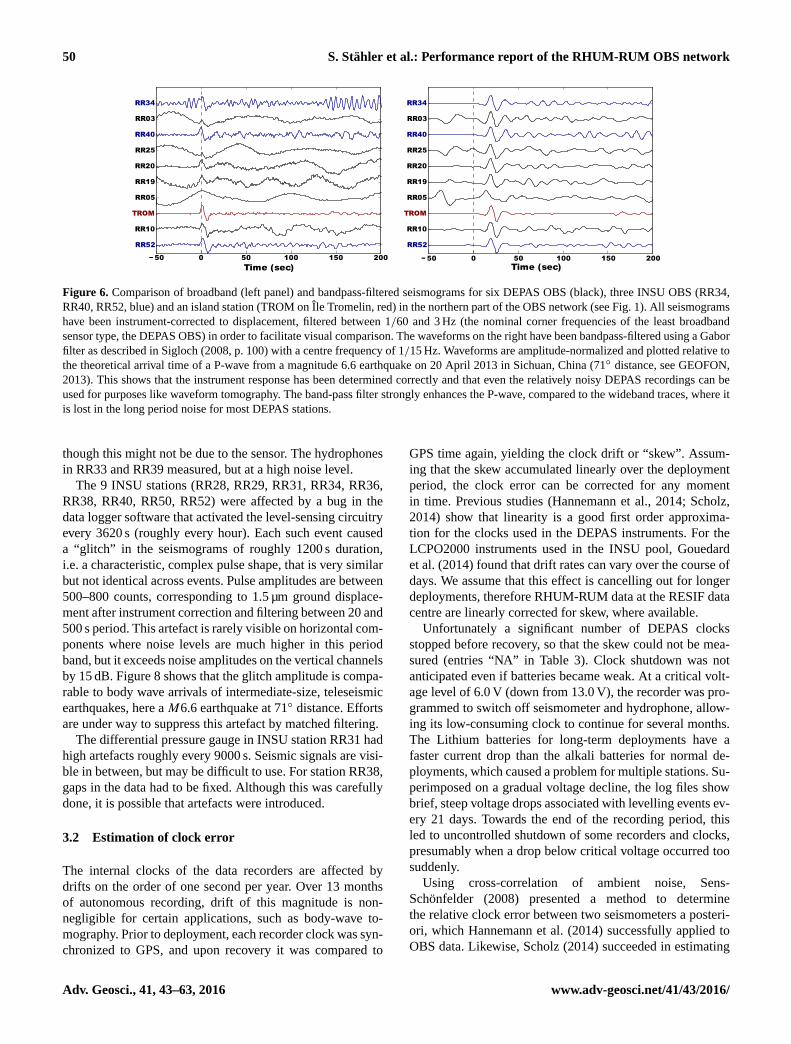
Figure 6. Comparison of broadband (left panel) and bandpass-filtered seismograms for six DEPAS OBS (black), three INSU OBS (RR34,

RR40, RR52, blue) and an island station (TROM on Île Tromelin, red) in the northern part of the OBS network (see Fig. 1). All seismograms

have been instrument-corrected to displacement, filtered between 1/60 and 3 Hz (the nominal corner frequencies of the least broadband

sensor type, the DEPAS OBS) in order to facilitate visual comparison. The waveforms on the right have been bandpass-filtered using a Gabor

filter as described in Sigloch (2008, p. 100) with a centre frequency of 1/15 Hz. Waveforms are amplitude-normalized and plotted relative to

the theoretical arrival time of a P-wave from a magnitude 6.6 earthquake on 20 April 2013 in Sichuan, China (71◦ distance, see GEOFON,

2013). This shows that the instrument response has been determined correctly and that even the relatively noisy DEPAS recordings can be

used for purposes like waveform tomography. The band-pass filter strongly enhances the P-wave, compared to the wideband traces, where it

is lost in the long period noise for most DEPAS stations.

though this might not be due to the sensor. The hydrophones

in RR33 and RR39 measured, but at a high noise level.

The 9 INSU stations (RR28, RR29, RR31, RR34, RR36,

RR38, RR40, RR50, RR52) were affected by a bug in the

data logger software that activated the level-sensing circuitry

every 3620 s (roughly every hour). Each such event caused

a “glitch” in the seismograms of roughly 1200 s duration,

i.e. a characteristic, complex pulse shape, that is very similar

but not identical across events. Pulse amplitudes are between

500–800 counts, corresponding to 1.5 µm ground displace-

ment after instrument correction and filtering between 20 and

500 s period. This artefact is rarely visible on horizontal com-

ponents where noise levels are much higher in this period

band, but it exceeds noise amplitudes on the vertical channels

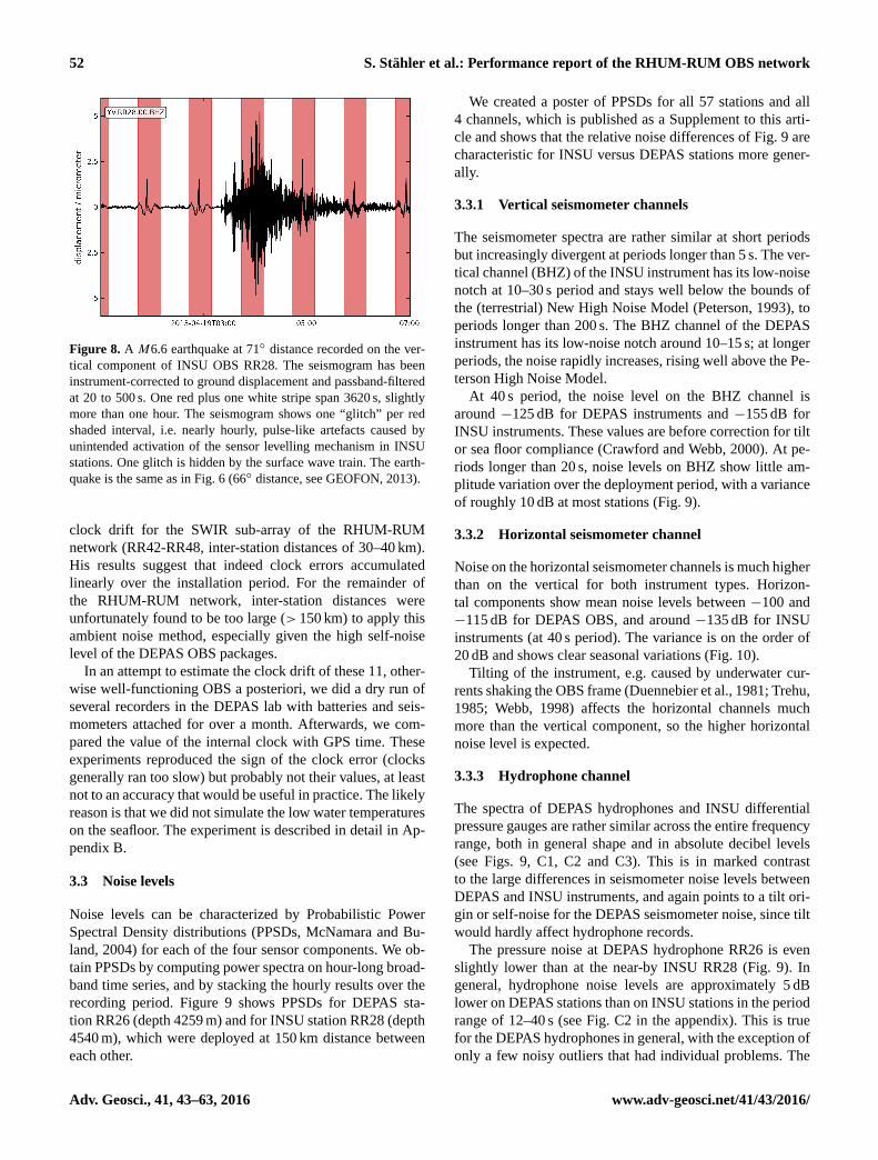
by 15 dB. Figure 8 shows that the glitch amplitude is compa-

rable to body wave arrivals of intermediate-size, teleseismic

earthquakes, here a M6.6 earthquake at 71◦ distance. Efforts

are under way to suppress this artefact by matched filtering.

The differential pressure gauge in INSU station RR31 had

high artefacts roughly every 9000 s. Seismic signals are visi-

ble in between, but may be difficult to use. For station RR38,

gaps in the data had to be fixed. Although this was carefully

done, it is possible that artefacts were introduced.

3.2 Estimation of clock error

The internal clocks of the data recorders are affected by

drifts on the order of one second per year. Over 13 months

of autonomous recording, drift of this magnitude is non-

negligible for certain applications, such as body-wave to-

mography. Prior to deployment, each recorder clock was syn-

chronized to GPS, and upon recovery it was compared to

GPS time again, yielding the clock drift or “skew”. Assum-

ing that the skew accumulated linearly over the deployment

period, the clock error can be corrected for any moment

in time. Previous studies (Hannemann et al., 2014; Scholz,

2014) show that linearity is a good first order approxima-

tion for the clocks used in the DEPAS instruments. For the

LCPO2000 instruments used in the INSU pool, Gouedard

et al. (2014) found that drift rates can vary over the course of

days. We assume that this effect is cancelling out for longer

deployments, therefore RHUM-RUM data at the RESIF data

centre are linearly corrected for skew, where available.

Unfortunately a significant number of DEPAS clocks

stopped before recovery, so that the skew could not be mea-

sured (entries “NA” in Table 3). Clock shutdown was not

anticipated even if batteries became weak. At a critical volt-

age level of 6.0 V (down from 13.0 V), the recorder was pro-

grammed to switch off seismometer and hydrophone, allow-

ing its low-consuming clock to continue for several months.

The Lithium batteries for long-term deployments have a

faster current drop than the alkali batteries for normal de-

ployments, which caused a problem for multiple stations. Su-

perimposed on a gradual voltage decline, the log files show

brief, steep voltage drops associated with levelling events ev-

ery 21 days. Towards the end of the recording period, this

led to uncontrolled shutdown of some recorders and clocks,

presumably when a drop below critical voltage occurred too

suddenly.

Using cross-correlation of ambient noise, Sens-

Schönfelder (2008) presented a method to determine

the relative clock error between two seismometers a posteri-

ori, which Hannemann et al. (2014) successfully applied to

OBS data. Likewise, Scholz (2014) succeeded in estimating



Station Oct. 2012 Nov. 2012 Dec. 2012 Jan. 2013 Feb. 2013 Mar. 2013 Apr. 2013 May 2013 Jun. 2013 Jul. 2013 Aug. 2013 Sep. 2013 Oct. 2013 Nov. 2013

RR01

RR02

RR03

RR04

RR05

RR06

RR07

RR08

RR09

RR10

RR11

RR12

RR13

RR14

RR15

RR16

RR17

RR18

RR19

RR20

RR21

RR22

RR23

RR24

RR25

RR26

RR27

RR28

RR29

RR30

RR31

RR32

RR33

RR34

RR35

RR36

RR37

RR38

RR39

RR40

RR41

RR42

RR43

RR44

RR45

RR46

RR47

RR48

RR49

RR50

RR51

RR52

RR53

RR54

RR55

RR56

RR57

No Skew

SHSHSHSHSHSHSHSHSHSHSHSHSHSHSHSHSHSHSHSHSHSHSHSHSHSHSHSHSHSHSHSHSHSHSHSHSHSHSHSHSHSHSHSHSHSHSHSHSHSHSHSHSHSHSHSHSH

No Skew

No Skew

No Skew

No Skew

No Skew

No Skew

No Skew

No Skew

No Skew

No Skew

No Skew

No Skew

No Skew

No Skew

No Skew

No Skew

No Skew

No Skew

No Skew

No Skew

No Skew

No Skew

No Skew

No Skew

DEPAS OBS

INSU OBS

Geomar OBS

120s instrument

channel fine

ch. record noisy

ch. record useless

no data recorded

data overwritten

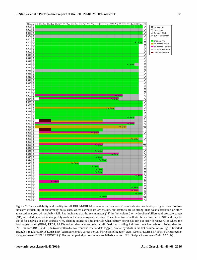
Figure 7. Data availability and quality for all RHUM-RHUM ocean-bottom stations. Green indicates availability of good data. Yellow

indicates availability of abnormally noisy data, where earthquakes are visible, but artefacts are so strong, that noise correlation or other

advanced analyses will probably fail. Red indicates that the seismometer (“S” in first column) or hydrophone/differential pressure gauge

(“H”) recorded data that is completely useless for seismological purposes. These time traces will still be archived at RESIF and may be

useful for analysis of error sources. Grey shading indicates time intervals when battery power had run out prior to recovery, or where the

data logger failed (RR02, RR04, RR15) and no data was recorded at all. Dark red shading indicates time intervals of missing data for

INSU stations RR31 and RR34 (overwritten due to erroneous reset of data logger). Station symbols in the last column follow Fig. 1. Inverted

Triangles: regular DEPAS LOBSTER (seismometer 60 s corner period, 50 Hz sampling rate); stars: Geomar LOBSTER (60 s, 50 Hz); regular

triangles: newer DEPAS LOBSTER (120 s corner period, all seismometers failed); circles: INSU/Scripps instrument (240 s, 62.5 Hz).



Figure 8. A M6.6 earthquake at 71◦ distance recorded on the ver-

tical component of INSU OBS RR28. The seismogram has been

instrument-corrected to ground displacement and passband-filtered

at 20 to 500 s. One red plus one white stripe span 3620 s, slightly

more than one hour. The seismogram shows one “glitch” per red

shaded interval, i.e. nearly hourly, pulse-like artefacts caused by

unintended activation of the sensor levelling mechanism in INSU

stations. One glitch is hidden by the surface wave train. The earth-

quake is the same as in Fig. 6 (66◦ distance, see GEOFON, 2013).

clock drift for the SWIR sub-array of the RHUM-RUM

network (RR42-RR48, inter-station distances of 30–40 km).

His results suggest that indeed clock errors accumulated

linearly over the installation period. For the remainder of

the RHUM-RUM network, inter-station distances were

unfortunately found to be too large (> 150 km) to apply this

ambient noise method, especially given the high self-noise

level of the DEPAS OBS packages.

In an attempt to estimate the clock drift of these 11, other-

wise well-functioning OBS a posteriori, we did a dry run of

several recorders in the DEPAS lab with batteries and seis-

mometers attached for over a month. Afterwards, we com-

pared the value of the internal clock with GPS time. These

experiments reproduced the sign of the clock error (clocks

generally ran too slow) but probably not their values, at least

not to an accuracy that would be useful in practice. The likely

reason is that we did not simulate the low water temperatures

on the seafloor. The experiment is described in detail in Ap-

pendix B.

3.3 Noise levels

Noise levels can be characterized by Probabilistic Power

Spectral Density distributions (PPSDs, McNamara and Bu-

land, 2004) for each of the four sensor components. We ob-

tain PPSDs by computing power spectra on hour-long broad-

band time series, and by stacking the hourly results over the

recording period. Figure 9 shows PPSDs for DEPAS sta-

tion RR26 (depth 4259 m) and for INSU station RR28 (depth

4540 m), which were deployed at 150 km distance between

each other.

We created a poster of PPSDs for all 57 stations and all

4 channels, which is published as a Supplement to this arti-

cle and shows that the relative noise differences of Fig. 9 are

characteristic for INSU versus DEPAS stations more gener-

ally.

3.3.1 Vertical seismometer channels

The seismometer spectra are rather similar at short periods

but increasingly divergent at periods longer than 5 s. The ver-

tical channel (BHZ) of the INSU instrument has its low-noise

notch at 10–30 s period and stays well below the bounds of

the (terrestrial) New High Noise Model (Peterson, 1993), to

periods longer than 200 s. The BHZ channel of the DEPAS

instrument has its low-noise notch around 10–15 s; at longer

periods, the noise rapidly increases, rising well above the Pe-

terson High Noise Model.

At 40 s period, the noise level on the BHZ channel is

around −125 dB for DEPAS instruments and −155 dB for

INSU instruments. These values are before correction for tilt

or sea floor compliance (Crawford and Webb, 2000). At pe-

riods longer than 20 s, noise levels on BHZ show little am-

plitude variation over the deployment period, with a variance

of roughly 10 dB at most stations (Fig. 9).

3.3.2 Horizontal seismometer channel

Noise on the horizontal seismometer channels is much higher

than on the vertical for both instrument types. Horizon-

tal components show mean noise levels between −100 and

−115 dB for DEPAS OBS, and around −135 dB for INSU

instruments (at 40 s period). The variance is on the order of

20 dB and shows clear seasonal variations (Fig. 10).

Tilting of the instrument, e.g. caused by underwater cur-

rents shaking the OBS frame (Duennebier et al., 1981; Trehu,

1985; Webb, 1998) affects the horizontal channels much

more than the vertical component, so the higher horizontal

noise level is expected.

3.3.3 Hydrophone channel

The spectra of DEPAS hydrophones and INSU differential

pressure gauges are rather similar across the entire frequency

range, both in general shape and in absolute decibel levels

(see Figs. 9, C1, C2 and C3). This is in marked contrast

to the large differences in seismometer noise levels between

DEPAS and INSU instruments, and again points to a tilt ori-

gin or self-noise for the DEPAS seismometer noise, since tilt

would hardly affect hydrophone records.

The pressure noise at DEPAS hydrophone RR26 is even

slightly lower than at the near-by INSU RR28 (Fig. 9). In

general, hydrophone noise levels are approximately 5 dB

lower on DEPAS stations than on INSU stations in the period

range of 12–40 s (see Fig. C2 in the appendix). This is true

for the DEPAS hydrophones in general, with the exception of

only a few noisy outliers that had individual problems. The



Figure 9. Probabilistic power spectral densities (PPSDs) for a DEPAS station (RR26, left column panels) and an INSU station (RR28, right

column panels). PPSDs are composed of hour-long power spectra stacked over the entire deployment interval. Colour marks the frequency

of occurrence of different noise levels, where purple indicates relatively rare, and red relatively frequent (McNamara and Buland, 2004).

Black curves mark the upper and lower bounds of the New High and Low Noise Model of Peterson (1993). The two instruments were

installed within 150 km of each other, in an abyssal plain 300 km south-west of La Réunion island (cf. Fig. 1). At periods longer than 5 s, the

INSU seismometers are much quieter than the DEPAS instrument (see Sect. 4). By contrast, the pressure channel BDH of the two models

(hydrophone for DEPAS, differential pressure gauge for INSU) shows very similar noise levels. A poster with PPSDs for all stations is

available on ResearchGate (Stähler et al., 2015) and as an Supplement to this paper.

overall lower noise level can probably be explained by com-

pletely different instrument types (hydrophones on DEPAS

versus differential pressure gauges on INSU stations).

3.4 Temporal noise variations

We expect two sources for temporal noise variations:

(1) varying wave heights due to storm activity, which af-

fects mostly the microseismic noise band. (2) Water current-

induced tilt, which creates long period noise.



Figure 10 shows the temporal evolution of noise levels

between October 2012 and October 2013 at DEPAS sta-

tion RR01 near La Réunion (depth 4298 m), between 2 and

60 s). In the secondary microseismic noise band (2–10 s pe-

riod), peak noise intervals coincide with cyclone passages

during southern summer (blue frames). Cyclones are tropi-

cal storms, the Indian Ocean equivalent of hurricanes and ty-

phoons. Their correlation to microseismic noise is most pro-

nounced on the BHZ component. In fact, Davy et al. (2014)

were able to track the path of a cyclone across the RHUM-

RUM network using recordings of secondary microseismic

noise only.

By contrast, peak noise episodes in the 20–60 s band show

no clear correlation with cyclone passages. Rather, the high-

est levels occur during southern winter (March to Septem-

ber), out of cyclone season. Seasonal variations in deep-

sea currents might explain tilt noise at these lower frequen-

cies. The HYCOM-based global ocean circulation model

(GLBa0.08/expt_90.9) (Cummings, 2005) does predict

more episodes of strong currents at RR01 during southern au-

tumn, (Fig. 10 bottom), but its absolute velocity values would

appear low for effectively shaking an OBS. However, global

ocean circulation models for this region have very poor reso-

lution in the bottom layer, so that true bottom currents may be

different. A recent measurement of current profiles at 23◦ S,

48◦ E (Ponsoni et al., 2015) suggests that bottom velocities

generally do not exceed a few cm per second in the region

(L. Ponsoni, personal communication, 2015). Unfortunately,

the nearest RHUM-RUM station, (RR23) failed to deliver

seismograms for comparison.

4 Discussion of the different noise levels

The relative stronger overall noise on the DEPAS instrument

affects the usability of the OBS for waveform tomography

and analysis of long-period waveforms. Hence its causes are

of interest to future users of the pool and for instrument de-

velopers. We discuss four potential differences between the

two instrument types:

The gimbal system: if the gimbal system were not stable

enough, it could cause additional noise on all compo-

nents. This hypothesis cannot be proven or falsified,

since the CMG-OBS40T cannot be tested outside its

gimbal. Experience shows that this would rather cause

high-frequency noise.

The data logger: the data loggers of the DEPAS and the

INSU OBS could have different self-noise levels.

Again, this cannot be tested, since we have no data from

other loggers available. But similar to the gimbal sys-

tem, this would rather affect the high-frequency end of

the spectrum, which is similar for both types.

OBS tilt: the integration of the seismometer into the OBS

frame makes the DEPAS instruments more susceptible

Figure 10. Seasonal changes in the noise levels on OBS RR01 near

La Réunion. Spectrograms of noise on the three seismometer com-

ponents, where noise is plotted as the median of daily probabilistic

power spectral densities. Blue boxes mark episodes of cyclone ac-

tivity, which correlates well with peak noise episodes in the micro-

seismic band (periods around 10 s), especially on the BHZ compo-

nent. At periods longer than 20 s, seismic noise peaks occur prefer-

entially in southern autumn (February–June), most evident on the

horizontal components. The global ocean circulation model HY-

COM GLBa0.08/expt_90.9, running from 3 January 2011 to 20 Au-

gust 2013 predicts more intervals of strong ocean-bottom currents

for southern autumn (bottom panel) – qualitatively consistent with

the hypothesis that ocean bottom currents cause long-period OBS

noise by tilting the seismic sensors.

to current-induced tilt. Seasonal variations on the noise

level of the horizontal channels can be seen in Fig. 10

and in the cloudy look of the PPSDs beyond 10 s in

Fig. 9. However, tilt noise should affect horizontal chan-

nels much more strongly than vertical ones, which is

indeed the case for the INSU instruments. For the DE-

PAS instruments, the vertical noise is too high to be ex-

plained by tilt alone.

Seismometer self noise: the CMG-OBS40T is a 60s wide-

band instrument, based on the 10 s CMG-40T. While

the self noise of the latter is below the New Low Noise

Model (NLNM) for periods shorter than 10s, onshore

experiments with one of the CMG-OBS40Ts showed

self noise of −140 dB at 10 s period, which is far above

the NLNM. This strongly suggests that the reduced

power consumption of the OBS40T comes at the price

of a significantly increased self-noise level. High self-

noise probably explains the larger part of the excessive

noise on the vertical channel in our experiment.



To summarize, we expect the high noise level of the DEPAS

instruments to be caused by a combination of tilt and instru-

ment self noise, where the former dominates the noise on the

horizontal channels and the latter the noise on the vertical

channel. The fact that the variability of noise on the horizon-

tal channels is comparable between the two instrument types

suggests that the susceptibility to currents is similar, albeit

slightly higher on the DEPAS instrument package. The usage

of a compact wideband sensor in the LOBSTER instruments

has the advantage of a much lower power consumption, at

the price of a strongly increased noise level beyond 10 s.

More detailed analysis of the effect of sensor integration

would require usage of a more broadband sensor in the DE-

PAS instrument package.

5 Conclusions

From October 2012 to November 2013, the RHUM-RUM

experiment deployed and successfully recovered 48 German

DEPAS and 9 French INSU broadband ocean-bottom seis-

mometers around La Réunion, western Indian Ocean, mak-

ing this the largest deployment of either instrument type,

and the only joint experiment. Overall network performance

was very satisfactory, but a number of technical issues have

been described here, including blocked levelling mecha-

nisms, data logger malfunctioning, and loss of clock synchro-

nization.

For the first time, we publish instrument response informa-

tion on the DEPAS OBS, which allows to calculate the true

ground displacement in a wide frequency range.

This shows that at periods longer than 10 s, the INSU OBS

are much quieter than the DEPAS instruments, on all three

seismometer components. No such difference in data quality

exists for the hydrophones and differential pressure gauges,

which both worked extremely reliably. The increased long-

period noise on the DEPAS seismometers can be explained

by the surprisingly high instrument self-noise on the all chan-

nels of the Güralp CMG-OBS40T sensors and partially by

a higher susceptibility to current-induced tilt of the whole

OBS.

In the microseismic noise band, peak noise intervals can

be attributed to tropical storm activity (cyclones), whereas

no clear correlation with cyclones was found at lower fre-

quencies, where tilt and self-noise dominates (20–60 s period

band). A possible cause for instrument tilt is the action of

ocean-bottom currents, which are predicted to peak in south-

ern winter just like the tilt noise, but global ocean circulation

models are not sufficiently constrained to test this hypothesis

in more detail.

The RHUM-RUM data set has been assigned FDSN net-

work code YV and will be freely available by the end of

2017. Data and detailed StationXML meta-data files are

hosted and served by the RESIF data centre in Grenoble

(http://portal.resif.fr/?RHUM-RUM-experiment&lang=en).


http://portal.resif.fr/?RHUM-RUM-experiment&lang=en


Appendix A: Instrument responses

While conceptually straightforward, instrument corrections

can be non-trivial in practice because filter description can

be complex, and their specifications must exactly match the

format expected by the software used to apply the correc-

tions.

A1 Seismometers

Assuming that the seismometer is a causal linear time-

invariant system, its response can be described by a series

of poles pm and zeros rn:

Ginst(f )= Sd,inst ·A0 ·

∏Nn=1 (2πif − rn)∏Mm=1 (2πif −pm)

. (A1)

In Eq. (A1), Sd,inst is the sensitivity at reference frequency

fr with dimension counts (ms−1)−1. A0 is a dimension-

less normalization constant, which normalizes G(f ) to 1 at

reference frequency fr. Following convention, we defined

fr= 1 Hz= (2π)−1 (rad s−1). The M poles pm and N zeros

rn describe the frequency-dependency of the response.

Values for each instrument can be queried sending its se-

rial number email to [email protected]. Note that these

data sheets contain the frequencies of the poles and ze-

ros in Hz, while the StationXML format prefers them in

rad s−1. All DEPAS seismometers that functioned had the

same M = 4 poles and N = 2 zeros as described in Ta-

ble A1a, with the exception of RR13 that had M = 5 (Ta-

ble A1b) and RR22 with M = 6 poles (Table A1c)1.

Poles and zeros characterize the first, analogue stage of an

instrument; subsequent digital filter stages characterize the

ADC (Analogue to Digital Converter) and digital processing

units of the data recorder. For the seismometers, the analogue

filter stages were obtained from the manufacturers Güralp

and Nanometrics, and are compared in Fig. 4.

We follow the SEED reference manual’s Appendix C (Ah-

ern et al., 2012) to describe the response G(f ) in frequency-

domain. The total transfer function is the product of complex

response functions for the instrument, ADC and FIR decima-

tion stages:

G(f )=Ginst(f ) ·GADC(f ) ·GFIR(f ). (A2)

The gain or sensitivity Sd,inst is channel specific and is

determined by Güralp before delivering the instrument. For

our instruments, a typical value is 1980 V(ms−1)−1 with an

instrument-specific variance of 15 V(ms−1)−1.

The analogue seismometer signal was converted to digital

counts by a SEND GEOLON-MCS data logger. This conver-

sion is assumed to have a flat response curve:

1For the 120 s instruments, the manufacturer lists the same

6 poles and 2 zeros as RR22, which is probably not correct, since

they describe a corner period of 60 s. But since none of those

recorded data, this should not be a problem to users of the data.

Table A1. (a) 4 poles and 2 zeros of the 60 s Güralp CMG-OBS40T

used in the German LOBSTER OBS. Can be applied to all 60 s sta-

tions but RR13 and RR22. (b) 5 poles and 2 zeros of the 60 s Güralp

CMG-OBS40T used in station RR13. (c) 6 poles and 2 zeros of the

60 s Güralp CMG-OBS40T used in station RR22. (d) 11 poles and

6 zeros of the Trillium 240OBS used in the French OBS at RR38,

RR50 and RR52. (e) 11 poles and 6 zeros of Trillium 240OBS

with a serial number below 400. Those were used in stations RR28,

RR29, RR31, RR34, RR36 and RR40.

Pole pm Zero rn

in rad s−1 in rad s−1

(a)

1/2 −0.074016± 0.07347 i 0

3/4 −502.65± 596.9 i –

(b)

1/2 −0.074016± 0.074016 i 0

3 −502.66 –

4 −1005.3 –

5 −1130.98 –

(c)

1/2 −0.074016± 0.074016 i 0

3 −471.24 –

4/5 −395.1± 850.69 i –

6 −2199.1 –

(d)

1/2 −0.018134± 0.018034 i 0

3 −84.4 −72.5

4 −180.2+ 224.4 i −163.3

5 −180.2− 224.4 i −251

6 −725 −3270

7 −1060 –

8 −4300 –

9 −5800 –

10/11 −4200± 4600 i –

(e)

1/2 −0.017699± 0.017604 i 0

3 −85.3 −72.5

4 −155.4+ 210.8 i −159.3

5 −155.4− 210.8 i −251

6 −713 −3270

7 −1140 –

8 −4300 –

9 −5800 –

10/11 −4300± 4400 i –

GADC(f )= Sd,ADC. (A3)

The sensitivity of this stage is Sd,ADC= 3.62× 105

counts V−1, resulting in an overall sensitivity for the LOB-

STER seismometers of roughly 7.4× 105 counts (m s−1)−1

at reference frequency fr= 1 Hz (see Fig. 4).


[email protected]


The decimation of the digital signal to the recording fre-

quency is described by a series of NFIR FIR decimation fil-

ters. The kth digital filter stage has Lk coefficients bl,k , dec-

imating an input signal of sampling rate 1ti . The total FIR

response is the product of the individual FIR stages:

GFIR(f )=

NFIR∏k=1

Sd,FIR,k

Lk∑l

bl,ke2πi1tk . (A4)

For the DEPAS instruments, the decimation from 512 kHz to

50 or 100 Hz is described by 8 (100 Hz) or 9 (50 Hz) FIR

stages of uniform sensitivity Sd,FIR,k = 1, such that the sen-

sitivity is only affected by the instrument and ADC stages.

The coefficients bl,k have been defined by DEPAS and are

included in the StationXML and dataless files. They create

the sharp cut-off at 90 % of the Nyquist frequency in Figs. 4

and 5.

The INSU Trillium-240OBS seismometers features

M = 12 poles pm and N = 5 zeros rn in its analogue stage

(see Tables A1d and e). The pm and rn were taken from

the Trillium-240 user guide, which applies to the 240OBS

as well. The sensitivity is Sd,inst= 598.45 V(ms−1)−1. This

is half the value specified in the user guide, since the OBS

were connected single-ended. The analogue gain is 0.225 for

the horizontal channels and 1.0 for the vertical channel, to

maximize the vertical sensitivity while avoiding clipping on

the horizontal channel. The sensitivity of the CS5321-2 A/D

converter is 1 165 080 counts V−1, resulting in an overall

sensitivity of 6.97× 107 counts(m s−1)−1 on the horizontal

and 1.57× 108 counts/(m s−1)−1 on the vertical channels,

both at reference frequency fr= 1 Hz. The decimation from

8000 to 62.5 Hz is implemented by 7 FIR stages of uniform

sensitivity.

A2 DEPAS hydrophones

The responses of the hydrophones and differential pressure

gauges are also given by Eq. (A2), though with a different

instrument response Ginst,h(f ), that has to be calculated sep-

arately for each instrument, as briefly explained here: a hy-

drophone measures pressure variations via a piezo element,

which has a sensitivity of Sd,hyd in V Pa−1. Below its cor-

ner frequency (typically in the kHz range), its equivalent cir-

cuit is a capacitor Chyd. Together with the input capacity

of the amplifier Camp, the system has the total capacitance

Ctotal=Camp Chyd

Camp+Chyd. With the input impedance R of the sen-

sor, the system forms a high-pass filter with a transfer func-

tion

Ginst,h(f )= Sd,hyd

RCtotal2πif

1+RCtotal2πif, (A5)

equivalent to Eq. (A1) with a single pole

p1 =−1

RCtotal

=−Camp+Chyd

RCampChyd

rad s−1 (A6)

and one zero r1= 0 rad s−1.

The capacitanceChyd is instrument-specific. The reference

value from the manufacturer HighTechInc is Chyd= 45 nF.

Before sale, every hydrophone is calibrated, which showed a

mean value Chyd= 56.3 nF with a sample standard deviation

of 3.5 nF amongst the 60 instruments in the DEPAS pool.

The input resistance R of the data logger was either 210 or

500 M�, depending on the instrument version.

The sensitivity Sh is different for each hydrophone,

around 185 µV Pa−1 with a sample standard deviation of

8 µV Pa−1 amongst the DEPAS instruments. DEPAS sup-

plied us with values for Sd, R and Chyd for each instru-

ment. From those, we calculated poles, zeros and sensitivi-

ties, which are listed in the dataless SEED and StationXML

files available from the RESIF data centre. Geomar instru-

ments were equipped with a similar hydrophone model, HTI-

01-PCA from the same manufacturer. Its nominal values is

Chyd= 50 nF and since no individually calibrated responses

were available, we used the average value of the other HTI-

01-PCA in the DEPAS pool, resulting in Sd= 199.5 µV Pa−1

and p1= 0.10774 rad s−1. This applies to the Geomar OBS

(RR33, RR39, RR53 and RR56) as well as to RR45 and

RR55, where Geomar hydrophones were attached to LOB-

STER OBS.

A3 INSU differential pressure gauges

Differential pressure gauges (DPGs, Cox et al., 1984) are

hand-manufactured in research laboratories and their sensi-

tivity and low-pass frequency are challenging to calibrate.

The DPGs in stations RR28 and RR29 were manually cali-

brated on land by comparing their impulse response to that

of an absolute pressure gauge in a vacuum jar. Since the low-

pass frequency is highly dependent on the viscosity of the

oil in the gauge and this viscosity may change with temper-

ature and pressure, it is not sure that these values accurately

reflect the instrument response at the seafloor, although vi-

sual comparison with the DEPAS hydrophone PPSDs does

not suggest significant error. The DPGs on the other sensors

were not calibrated and the instrument responses given are

therefore the same as those for station RR28. This practice

is the same as that used by other OBS facilities (e.g. Godin

et al., 2013), but it leaves a significant uncertainty in the con-

verted signal amplitudes.

Appendix B: Description of laboratory experiments on

the DEPAS clocks

Since the internal clocks of several DEPAS OBS stopped be-

fore retrieval, and ambient noise estimation of the clock er-

ror proved impossible, we tried to estimate the clock error



from laboratory experiments. Hence we re-ran several data

recorders after their return to the DEPAS lab at AWI Bremer-

haven, in an attempt to measure their clock drifts. Only seven

data loggers were available (RR06, RR11, RR41, RR43,

RR44, RR45, RR55); the remainder had been redeployed in

new experiments. Attached to their original lithium batter-

ies and a seismometer, the recorders were run for 7 days, and

then for another 33 days. Table B1 shows the skews measured

after the two runs, linearly extrapolated to a hypothetical run

time of 365 days.

For 6 out of 7 stations, skew values from the two runs agree

to within less than 0.1 s. The exception is RR44, where the

skews disagree by more than one second (−0.50 s from the

7-day run, versus +0.55 s from the 33-day run). For RR11, a

skew of +0.61 s had been obtained upon OBS recovery (see

Table 3), as compared to −0.15 and −0.21 s in the two lab

runs (Table B1), which means mutual consistence to within

0.8 s, an uncertainty as large as the skew estimates them-

selves. No skew upon recovery was available for the remain-

ing six recorders.

Most lab skew values in Table B1 are rather small in mag-

nitude, compared to skews obtained during the field cam-

paign in Table 3. This pattern is consistent with the direct

comparison available for RR11, and hints at a systematic dif-

ference between seafloor runs and lab runs. In either setting,

the clocks tend to run too fast, as indicated by mostly posi-

tive skew values (upon recovery, the elapsed recorder time is

larger than the elapsed GPS time). But clocks on the seafloor

ran even faster than clocks in the lab. (Note that only DEPAS

stations in Table 3 should enter this comparison, since INSU

recorders are of a different make.)

The likely shortcoming of our lab experiments is that we

did not simulate temperature conditions of the real experi-

ment: a sudden drop from 22 to 4 ◦C) upon deployment, a

constant 4 ◦C during recording, and sudden warming to 22 ◦C

upon recovery. Solid-state oscillators are known to be tem-

perature dependent, which may explain why our lab experi-

ments could match the field observations qualitatively (cor-

rect sign of skew), but probably did not yield the correct skew

magnitudes. Hence we assign low confidence to the skew

measurements in Table B1 and do not apply any skew cor-

rections to RHUM-RUM time series based on these values.

Table B1. Lab measurements of clock skews for seven DEPAS

recorders. Two separate runs of 7 and 33 days durations yielded

skew measurements that are linearly extrapolated to a hypothetical

run of 365 days duration (for convenient comparison to skews mea-

sured in the field campaign, Table 3). We assign low confidence to

these lab measurements (see text for discussion) and do not correct

RHUM-RUM time series using these values.

Station Serial number Skew prediction for 365 days

(data logger) from 7 day exp. from 33 day exp.

RR06 060744 0.15 s 0.13 s

RR11 060753 −0.15 s −0.21 s

RR41 050922 0.3 s 0.23 s

RR43 060702 0.00 s 0.033 s

RR44 060751 −0.5 s 0.55 s

RR45 080104 0.045 s −0.05 s

RR55 060748 0.0015 s −0.03 s

Appendix C: Summary charts of noise levels across the

RHUM-RUM OBS network

Figures C1 to C3 are graphical summaries of noise statistics

for all stations and components, in three different frequency

bands:

Fig. C1: microseismic noise band (period range 5–15 s).

DEPAS and INSU seismometers record comparable

noise levels.

Fig. C2: low-noise notch (period band 15–40 s). The noise

level of the INSU seismometers is on average 15 dB

lower than the values for the DEPAS instruments.

Fig. C3: long-period band (40–100 s). Both INSU seis-

mometers (corner period 240 s) and the DEPAS seis-

mometers (corner period 60 s) still have nominal in-

strument sensitivity in this band, but the self-noise of

the Güralp instruments used in the DEPAS OBS is pro-

nounced, especially on the BHZ channel.

Probabilistic Power Spectral Densities (cf. Fig. 9) were

calculated for all stations and broadband components (BH1,

BH2, BHZ, BDH) by stacking hour-long time series. For

each of the three frequency bands, we averaged the hourly

spectra over the frequencies contained the band of interest,

and calculated the median, quartiles, 2.5 % percentile, and

97.5 % percentile power levels of the hourly band averages.

These statistics are plotted for all stations, components and

frequency bands in Figs. C1 to C3.



RR

01

RR

02

RR

03

RR

04

RR

05

RR

06

RR

07

RR

08

RR

09

RR

10

RR

11

RR

12

RR

13

RR

14

RR

15

RR

16

RR

17

RR

18

RR

19

RR

20

RR

21

RR

22

RR

23

RR

24

RR

25

RR

26

RR

27

RR

28

RR

29

RR

30

RR

31

RR

32

RR

33

RR

34

RR

35

RR

36

RR

37

RR

38

RR

39

RR

40

RR

41

RR

42

RR

43

RR

44

RR

45

RR

46

RR

47

RR

48

RR

49

RR

50

RR

51

RR

52

RR

53

RR

54

RR

55

RR

56

RR

57

Station name

-80

-60

-40

-20

0

20

40

60

Pow

er

/ dB

(1

0lo

g1

0[P

a2

/Hz]

)B

DH

, (2, 1

2) s

RR

01

RR

02

RR

03

RR

04

RR

05

RR

06

RR

07

RR

08

RR

09

RR

10

RR

11

RR

12

RR

13

RR

14

RR

15

RR

16

RR

17

RR

18

RR

19

RR

20

RR

21

RR

22

RR

23

RR

24

RR

25

RR

26

RR

27

RR

28

RR

29

RR

30

RR

31

RR

32

RR

33

RR

34

RR

35

RR

36

RR

37

RR

38

RR

39

RR

40

RR

41

RR

42

RR

43

RR

44

RR

45

RR

46

RR

47

RR

48

RR

49

RR

50

RR

51

RR

52

RR

53

RR

54

RR

55

RR

56

RR

57

Station name

-200

-180

-160

-140

-120

-100

-80

-60

Pow

er

/ dB

(1

0lo

g1

0[(

m2

/s4

)/H

z])

BH

1, (2

, 12) s

RR

01

RR

02

RR

03

RR

04

RR

05

RR

06

RR

07

RR

08

RR

09

RR

10

RR

11

RR

12

RR

13

RR

14

RR

15

RR

16

RR

17

RR

18

RR

19

RR

20

RR

21

RR

22

RR

23

RR

24

RR

25

RR

26

RR

27

RR

28

RR

29

RR

30

RR

31

RR

32

RR

33

RR

34

RR

35

RR

36

RR

37

RR

38

RR

39

RR

40

RR

41

RR

42

RR

43

RR

44

RR

45

RR

46

RR

47

RR

48

RR

49

RR

50

RR

51

RR

52

RR

53

RR

54

RR

55

RR

56

RR

57

Station name

-200

-180

-160

-140

-120

-100

-80

-60

Pow

er

/ dB

(1

0lo

g1

0[(

m2

/s4

)/H

z])

BH

2, (2

, 12) s

RR

01

RR

02

RR

03

RR

04

RR

05

RR

06

RR

07

RR

08

RR

09

RR

10

RR

11

RR

12

RR

13

RR

14

RR

15

RR

16

RR

17

RR

18

RR

19

RR

20

RR

21

RR

22

RR

23

RR

24

RR

25

RR

26

RR

27

RR

28

RR

29

RR

30

RR

31

RR

32

RR

33

RR

34

RR

35

RR

36

RR

37

RR

38

RR

39

RR

40

RR

41

RR

42

RR

43

RR

44

RR

45

RR

46

RR

47

RR

48

RR

49

RR

50

RR

51

RR

52

RR

53

RR

54

RR

55

RR

56

RR

57

Station name

-200

-180

-160

-140

-120

-100

-80

-60

Pow

er

/ dB

(1

0lo

g1

0[(

m2

/s4

)/H

z])

BH

Z, (2

, 12) s

Figure C1. Noise power levels in the microseismic noise band (5–15 s period), on the BH1, BH2, BHZ, and BDH components (4 sub-plots).

57 box plots per panel characterize the 57 RHUM-RUM stations. In each box plot, the red line marks the median power level during the

interval of successful recording. Top and bottom edges of the blue box mark the ranges of the two quartiles, and dashed line the range that

contains 95 % of all hourly observations in this frequency band (from 2.5 to 97.5 % percentile). Light blue shading indicates INSU stations,

all others are DEPAS or Geomar. Red shading indicates failed components. Grey horizontal band marks the power range bracketed by the

(terrestrial) New Low Noise and New High Noise Models (Peterson, 1993), in the frequency passband considered here.



RR

01

RR

02

RR

03

RR

04

RR

05

RR

06

RR

07

RR

08

RR

09

RR

10

RR

11

RR

12

RR

13

RR

14

RR

15

RR

16

RR

17

RR

18

RR

19

RR

20

RR

21

RR

22

RR

23

RR

24

RR

25

RR

26

RR

27

RR

28

RR

29

RR

30

RR

31

RR

32

RR

33

RR

34

RR

35

RR

36

RR

37

RR

38

RR

39

RR

40

RR

41

RR

42

RR

43

RR

44

RR

45

RR

46

RR

47

RR

48

RR

49

RR

50

RR

51

RR

52

RR

53

RR

54

RR

55

RR

56

RR

57

Station name

-80

-60

-40

-20

0

20

40

60Pow

er

/ dB

(1

0lo

g1

0[P

a2

/Hz]

)B

DH

, (12

, 40) s

RR

01

RR

02

RR

03

RR

04

RR

05

RR

06

RR

07

RR

08

RR

09

RR

10

RR

11

RR

12

RR

13

RR

14

RR

15

RR

16

RR

17

RR

18

RR

19

RR

20

RR

21

RR

22

RR

23

RR

24

RR

25

RR

26

RR

27

RR

28

RR

29

RR

30

RR

31

RR

32

RR

33

RR

34

RR

35

RR

36

RR

37

RR

38

RR

39

RR

40

RR

41

RR

42

RR

43

RR

44

RR

45

RR

46

RR

47

RR

48

RR

49

RR

50

RR

51

RR

52

RR

53

RR

54

RR

55

RR

56

RR

57

Station name

-200

-180

-160

-140

-120

-100

-80

-60

Pow

er

/ dB

(1

0lo

g1

0[(

m2

/s4

)/H

z])

BH

1, (1

2, 4

0) s

RR

01

RR

02

RR

03

RR

04

RR

05

RR

06

RR

07

RR

08

RR

09

RR

10

RR

11

RR

12

RR

13

RR

14

RR

15

RR

16

RR

17

RR

18

RR

19

RR

20

RR

21

RR

22

RR

23

RR

24

RR

25

RR

26

RR

27

RR

28

RR

29

RR

30

RR

31

RR

32

RR

33

RR

34

RR

35

RR

36

RR

37

RR

38

RR

39

RR

40

RR

41

RR

42

RR

43

RR

44

RR

45

RR

46

RR

47

RR

48

RR

49

RR

50

RR

51

RR

52

RR

53

RR

54

RR

55

RR

56

RR

57

Station name

-200

-180

-160

-140

-120

-100

-80

-60

Pow

er

/ dB

(1

0lo

g1

0[(

m2

/s4

)/H

z])

BH

2, (1

2, 4

0) s

RR

01

RR

02

RR

03

RR

04

RR

05

RR

06

RR

07

RR

08

RR

09

RR

10

RR

11

RR

12

RR

13

RR

14

RR

15

RR

16

RR

17

RR

18

RR

19

RR

20

RR

21

RR

22

RR

23

RR

24

RR

25

RR

26

RR

27

RR

28

RR

29

RR

30

RR

31

RR

32

RR

33

RR

34

RR

35

RR

36

RR

37

RR

38

RR

39

RR

40

RR

41

RR

42

RR

43

RR

44

RR

45

RR

46

RR

47

RR

48

RR

49

RR

50

RR

51

RR

52

RR

53

RR

54

RR

55

RR

56

RR

57

Station name

-200

-180

-160

-140

-120

-100

-80

-60

Pow

er

/ dB

(1

0lo

g1

0[(

m2

/s4

)/H

z])

BH

Z, (1

2, 4

0) s

Figure C2. Noise power levels in the band of the low-noise notch (15–40 s period). Refer to the caption of Fig. C1 for explanation.



RR

01

RR

02

RR

03

RR

04

RR

05

RR

06

RR

07

RR

08

RR

09

RR

10

RR

11

RR

12

RR

13

RR

14

RR

15

RR

16

RR

17

RR

18

RR

19

RR

20

RR

21

RR

22

RR

23

RR

24

RR

25

RR

26

RR

27

RR

28

RR

29

RR

30

RR

31

RR

32

RR

33

RR

34

RR

35

RR

36

RR

37

RR

38

RR

39

RR

40

RR

41

RR

42

RR

43

RR

44

RR

45

RR

46

RR

47

RR

48

RR

49

RR

50

RR

51

RR

52

RR

53

RR

54

RR

55

RR

56

RR

57

Station name

-80

-60

-40

-20

0

20

40

60Pow

er

/ dB

(1

0lo

g1

0[P

a2

/Hz]

)B

DH

, (40

, 10

0) s

RR

01

RR

02

RR

03

RR

04

RR

05

RR

06

RR

07

RR

08

RR

09

RR

10

RR

11

RR

12

RR

13

RR

14

RR

15

RR

16

RR

17

RR

18

RR

19

RR

20

RR

21

RR

22

RR

23

RR

24

RR

25

RR

26

RR

27

RR

28

RR

29

RR

30

RR

31

RR

32

RR

33

RR

34

RR

35

RR

36

RR

37

RR

38

RR

39

RR

40

RR

41

RR

42

RR

43

RR

44

RR

45

RR

46

RR

47

RR

48

RR

49

RR

50

RR

51

RR

52

RR

53

RR

54

RR

55

RR

56

RR

57

Station name

-200

-180

-160

-140

-120

-100

-80

-60

Pow

er

/ dB

(1

0lo

g1

0[(

m2

/s4

)/H

z])

BH

1, (4

0, 1

00

) s

RR

01

RR

02

RR

03

RR

04

RR

05

RR

06

RR

07

RR

08

RR

09

RR

10

RR

11

RR

12

RR

13

RR

14

RR

15

RR

16

RR

17

RR

18

RR

19

RR

20

RR

21

RR

22

RR

23

RR

24

RR

25

RR

26

RR

27

RR

28

RR

29

RR

30

RR

31

RR

32

RR

33

RR

34

RR

35

RR

36

RR

37

RR

38

RR

39

RR

40

RR

41

RR

42

RR

43

RR

44

RR

45

RR

46

RR

47

RR

48

RR

49

RR

50

RR

51

RR

52

RR

53

RR

54

RR

55

RR

56

RR

57

Station name

-200

-180

-160

-140

-120

-100

-80

-60

Pow

er

/ dB

(1

0lo

g1

0[(

m2

/s4

)/H

z])

BH

2, (4

0, 1

00

) s

RR

01

RR

02

RR

03

RR

04

RR

05

RR

06

RR

07

RR

08

RR

09

RR

10

RR

11

RR

12

RR

13

RR

14

RR

15

RR

16

RR

17

RR

18

RR

19

RR

20

RR

21

RR

22

RR

23

RR

24

RR

25

RR

26

RR

27

RR

28

RR

29

RR

30

RR

31

RR

32

RR

33

RR

34

RR

35

RR

36

RR

37

RR

38

RR

39

RR

40

RR

41

RR

42

RR

43

RR

44

RR

45

RR

46

RR

47

RR

48

RR

49

RR

50

RR

51

RR

52

RR

53

RR

54

RR

55

RR

56

RR

57

Station name

-200

-180

-160

-140

-120

-100

-80

-60

Pow

er

/ dB

(1

0lo

g1

0[(

m2

/s4

)/H

z])

BH

Z, (4

0, 1

00

) s

Figure C3. Noise power levels in the long-period band (40–100 s period). Refer to the caption of Fig. C1 for explanation.



The Supplement related to this article is available online

at doi:10.5194/adgeo-4-43-2016-supplement.

Author contributions. K. Hosseini, M. Tsekhmistrenko, K.

Sigloch, S. C. Stähler, W. C. Crawford, J.-R. Scholz and A. Maz-

zullo processed raw data and assessed station performance during

and after the OBS recovery cruise. Station meta-data were as-

sembled and verified for the DEPAS instruments by S. C. Stähler

and M. C. Schmidt-Aursch, and for the INSU instruments by

W. C. Crawford. A. Mazzullo, M. Deen and W. C. Crawford

investigated the “glitch” on the INSU instruments. G. Barruol and

K. Sigloch designed the RHUM-RUM project, obtained funding

for the OBS experiment, and led the cruises. S. C. Stähler and

K. Sigloch prepared the manuscript with contributions from all

co-authors.

Acknowledgements. RHUM-RUM is funded by Deutsche

Forschungsgemeinschaft (grants SI1538/2-1 and SI1538/4-1) and

Agence National de la Recherche (project ANR-11-BS56-0013).

Additional support is provided by Centre National de la Recherche

Scientifique-Institut National des Sciences de l’Univers, Terres

Australes et Antarctiques Françaises, Institut Polaire Paul Emile

Victor, Alfred Wegener Institute Bremerhaven, and a Marie Curie

Career Integration Grant to K. Sigloch. Instruments were provided

by “Deutscher Geräte-Pool für Amphibische Seismologie” at

Alfred-Wegener-Institut, Bremerhaven, “Parc Sismomètre fond du

mer” at INSU/IPGP, and Geomar, Kiel. We thank Erik Labahn,

Henning Kirk, and the crews of research vessels Marion Dufresne

and Meteor for excellent support during deployment and recovery.

We thank Carlos Corela for preparing the initial compilation

of the DEPAS metadata. Ulf Gräwe assisted with downloading

HYCOM ocean model data (http://hycom.org). All figures were

produced with the ObsPy software, version 0.10.2 (The ObsPy

Development Team, 2015). We thank the RESIF data centre in

Grenoble, especially Catherine Pequegnat and Pierre Volcke, for

hosting the RHUM-RUM data.

RESIF is supported by the French Ministry of Education

and Research, by 18 Research Institutions and Universities in

France, by the French National Research Agency (ANR) as part

of the “Investissements d’Avenir” program (reference: ANR-11-

EQPX-0040) and by the French Ministry of Ecology, Sustainable

Development and Energy.

Edited by: D. Pesaresi

Reviewed by: D. Suetsugu and three anonymous referees

References

Ahern, T. K., Casey, R., Barnes, D., Benson, R., and Knight,

T.: Seed Reference Manual, Tech. rep., Incorporated Re-

search Institutions for Seismology, http://www.fdsn.org/media/

_s/publications/SEEDManual_V2.4.pdf (last access: 19 Octo-

ber 2015), 2012.

Barruol, G.: PLUME investigates South Pacific Super-

swell, Eos, Trans. Am. Geophys. Union, 83, 511,

doi:10.1029/2002EO000354, 2002.

Barruol, G. and Sigloch, K.: Investigating La Réunion hot spot from

crust to core, Eos, Trans. Am. Geophys. Union, 94, 205–207,

doi:10.1002/2013EO230002, 2013.

Barruol, G., Sigloch, K., and the RHUM-RUM group: RHUM-

RUM experiment, 2011–2015, code YV (Réunion Hotspot and

Upper Mantle – Réunion’s Unterer Mantel) funded by ANR,

DFG, CNRS-INSU, IPEV, TAAF, instrumented by DEPAS,

INSU-OBS, AWI and the Universities of Muenster, Bonn, La

Réunion, doi:10.15778/RESIF.YV2011, 2011.

Becker, J. J., Sandwell, D. T., Smith, W. H. F., Braud, J., Binder, B.,

Depner, J., Fabre, D., Factor, J., Ingalls, S., Kim, S.-H., Ladner,

R., Marks, K., Nelson, S., Pharaoh, A., Trimmer, R., Von Rosen-

berg, J., Wallace, G., and Weatherall, P.: Global Bathymetry and

Elevation Data at 30 Arc Seconds Resolution: SRTM30_PLUS,

Mar. Geodyn., 32, 355–371, doi:10.1080/01490410903297766,

2009.

Cannat, M., Rommevaux-Jestin, C., Sauter, D., Deplus, C., and

Mendel, V.: Formation of the axial relief at the very slow spread-

ing Southwest Indian Ridge (49◦ to 69◦ E), J. Geophys. Res.,

104, 22825, doi:10.1029/1999JB900195, 1999.

Cox, C., Deaton, T., and Webb, S.: A Deep-Sea Differen-

tial Pressure Gauge, J. Atmos. Ocean. Tech., 1, 237–246,

doi:10.1175/1520-0426(1984)001<0237:ADSDPG>2.0.CO;2,

1984.

Crawford, W. C. and Webb, S. C.: Identifying and Remov-

ing Tilt Noise from Low-Frequency (< 0.1 Hz) Seafloor Ver-

tical Seismic Data, Bull. Seismol. Soc. Am., 90, 952–963,

doi:10.1785/0119990121, 2000.

Cummings, J. A.: Operational multivariate ocean data as-

similation, Q. J. Roy. Meteorol. Soc., 131, 3583–3604,

doi:10.1256/qj.05.105, 2005.

Dahm, T., Thorwart, M., Flueh, E. R., Braun, T., Herber, R.,

Favali, P., Beranzoli, L., D’Anna, G., Frugoni, F., and Sm-

riglio, G.: Ocean bottom seismometers deployed in Tyrrhe-

nian Sea, Eos, Trans. Am. Geophys. Union, 83, 309,

doi:10.1029/2002EO000221, 2002.

Davy, C., Barruol, G., Fontaine, F. R., Sigloch, K., and Stutzmann,

E.: Tracking major storms from microseismic and hydroacous-

tic observations on the seafloor, Geophys. Res. Lett., 41, 8825–

8831, doi:10.1002/2014GL062319, 2014.

Duennebier, F. K., Blackinton, G., and Sutton, G. H.: Current-

generated noise recorded on ocean bottom seismometers, Mar.

Geophys. Res., 5, 109–115, doi:10.1007/BF00310316, 1981.

Dyment, J., Lin, J., and Baker, E.: Ridge-Hotspot Interactions:

What Mid-Ocean Ridges Tell Us About Deep Earth Processes,

Oceanography, 20, 102–115, doi:10.5670/oceanog.2007.84,

2007.

Flueh, E. R. and Biolas, J.: A digital, high data capacity ocean bot-

tom recorder for seismic investigations, Int. Underw. Syst. Des.,

18, 18–20, 1996.


http://dx.doi.org/10.5194/adgeo-4-43-2016-supplement

http://hycom.org

http://www.fdsn.org/media/_s/publications/SEEDManual_V2.4.pdf

http://www.fdsn.org/media/_s/publications/SEEDManual_V2.4.pdf

http://dx.doi.org/10.1029/2002EO000354

http://dx.doi.org/10.1002/2013EO230002

http://dx.doi.org/10.15778/RESIF.YV2011

http://dx.doi.org/10.1080/01490410903297766

http://dx.doi.org/10.1029/1999JB900195

http://dx.doi.org/10.1175/1520-0426(1984)001<0237:ADSDPG>2.0.CO;2

http://dx.doi.org/10.1785/0119990121

http://dx.doi.org/10.1256/qj.05.105

http://dx.doi.org/10.1029/2002EO000221

http://dx.doi.org/10.1002/2014GL062319

http://dx.doi.org/10.1007/BF00310316

http://dx.doi.org/10.5670/oceanog.2007.84


Geissler, W. H. and Schmidt, R.: Short Cruise Report

Maria S. Merian; MSM 24 Walvis Bay – Cape Town,

Tech. rep., Leitstelle Deutsche Forschungsschiffe, Ham-

burg, https://www.ldf.uni-hamburg.de/merian/wochenberichte/

wochenberichte-merian/msm22-msm25/msm24-scr.pdf (last

access: 19 October 2015), 2013.

Geissler, W. H., Matias, L., Stich, D., Carrilho, F., Jokat, W., Monna,

S., Ibenbrahim, A., Mancilla, F., Gutscher, M. A., Sallars, V., and

Zitellini, N.: Focal mechanisms for sub-crustal earthquakes in

the Gulf of Cadiz from a dense OBS deployment, Geophys. Res.

Lett., 37, 7–12, doi:10.1029/2010GL044289, 2010.

GEOFON: Mw 6.6 earthquake, Sichuan China, 2013-04-20

(Moment Tensor Solution), doi:10.5880/GEOFON.gfz2013hrdy,

2013.

Godin, O. A., Zabotin, N. A., Sheehan, A. F., Yang, Z., and Collins,

J. A.: Power spectra of infragravity waves in a deep ocean, Geo-

phys. Res. Lett., 40, 2159–2165, doi:10.1002/grl.50418, 2013.

Gouedard, P., Seher, T., McGuire, J. J., Collins, J. A., and van der

Hilst, R.: Correction of Ocean-Bottom Seismometer Instrumen-

tal Clock Errors Using Ambient Seismic Noise, Bull. Seismol.

Soc. Am., 104, doi:10.1785/0120130157, 2014.

Hannemann, K., Krüger, F., and Dahm, T.: Measuring of clock

drift rates and static time offsets of ocean bottom stations by

means of ambient noise, Geophys. J. Int., 196, 1034–1042,

doi:10.1093/gji/ggt434, 2014.

Laske, G., Collins, J. A., Wolfe, C. J., Solomon, S. C., Detrick,

R. S., Orcutt, J. A., Bercovici, D., and Hauri, E. H.: Probing

the Hawaiian Hot Spot With New Broadband Ocean Bottom

Instruments, Eos, Trans. Am. Geophys. Union, 90, 362–363,

doi:10.1029/2009EO410002, 2009.

McNamara, D. E. and Buland, R.: Ambient Noise Levels in the

Continental United States, Bull. Seismol. Soc. Am., 94, 1517–

1527, doi:10.1785/012003001, 2004.

Meier, T., Friederich, W., Papazachos, C., Taymaz, T., and Kind,

R.: EGELADOS: a temporary amphibian broadband seismic net-

work in the southern Aegean, in: Geophys. Res. Abstr., 9, 9020,

2007.

Morgan, W. J.: Rodriguez, Darwin, Amsterdam, . . . , A sec-

ond type of Hotspot Island, J. Geophys. Res., 83, 5355,

doi:10.1029/JB083iB11p05355, 1978.

Peterson, J.: Observations and Modeling of Seismic Background

Noise, Tech. rep., USGS, Albuquerque, New Mexico, 1993.

Ponsoni, L., Aguiar-González, B., Maas, L., van Aken, H.,

and Ridderinkhof, H.: Long-term observations of the east

madagascar undercurrent, Deep-Sea Res. Pt. I, 100, 64–78,

doi:10.1016/j.dsr.2015.02.004, 2015.

Scholz, J.-R.: Local seismicity of the segment-8-volcano at the

ultraslow spreading Southwest Indian Ridge, Diploma thesis,

Technische Universität Dresden, Dresden, 2014.

Sens-Schönfelder, C.: Synchronizing seismic networks with ambi-

ent noise, Geophys. J. Int., 174, 966–970, doi:10.1111/j.1365-

246X.2008.03842.x, 2008.

Sigloch, K.: Multiple-frequency body-wave tomography, PhD the-

sis, Princeton, 2008.

Stähler, S. C., Sigloch, K., Barruol, G., and Crawford, W. C.:

Noise levels at all stations of the RHUM-RUM OBS network,

doi:10.13140/RG.2.1.1374.0886, 2015.

Suetsugu, D., Sugioka, H., Isse, T., Fukao, Y., Shiobara, H.,

Kanazawa, T., Barruol, G., Schindelé, F., Reymond, D., Bon-

neville, A., and Debayle, E.: Probing South Pacific mantle

plumes with ocean bottom seismographs, Eos, Trans. Am. Geo-

phys. Union, 86, 429, doi:10.1029/2005EO440001, 2005.

Suetsugu, D., Shiobara, H., Sugioka, H., Ito, A., Isse, T., Kasaya,

T., Tada, N., Baba, K., Abe, N., Hamano, Y., Tarits, P., Barriot,

J.-P., and Reymond, D.: TIARES Project – Tomographic investi-

gation by seafloor array experiment for the Society hotspot, Earth

Planets Space, 64, i–iv, doi:10.5047/eps.2011.11.002, 2012.

Sumy, D. F., Lodewyk, J. A., Woodward, R. L., and Ev-

ers, B.: Ocean-Bottom Seismograph Performance during the

Cascadia Initiative, Seismol. Res. Lett., 86, 1238–1246,

doi:10.1785/0220150110, 2015.

The ObsPy Development Team: ObsPy 0.10.2,

doi:10.5281/zenodo.17641, 2015.

Tilmann, F., Yuan, X., Rümpker, G., and Rindraharisaona,

E.: SELASOMA Project, Madagascar 2012–2014,

doi:10.14470/MR7567431421, 2012.

Trehu, A. M.: A note on the effect of bottom currents on an ocean

bottom seismometer, Bull. Seismol. Soc. Am., 75, 1195–1204,

1985.

Webb, S. C.: Broadband seismology and noise under the ocean, Rev.

Geophys., 36, 105, doi:10.1029/97RG02287,1998.

Wolfe, C. J., Solomon, S. C., Laske, G., Collins, J. A., Detrick, R. S.,

Orcutt, J. A., Bercovici, D., and Hauri, E. H.: Mantle Shear-Wave

Velocity Structure Beneath the Hawaiian Hot Spot, Science, 326,

1388–1390, doi:10.1126/science.1180165, 2009.

Wysession, M., Wiens, D., Nyblade, A., and Rambolamanana,

G.: Investigating Mantle Structure with Broadband Seismic Ar-

rays in Madagascar and Mozambique, AGU Fall Meet. Abstr.,

p. B2591, 2012.


https://www.ldf.uni-hamburg.de/merian/wochenberichte/wochenberichte-merian/msm22-msm25/msm24-scr.pdf

https://www.ldf.uni-hamburg.de/merian/wochenberichte/wochenberichte-merian/msm22-msm25/msm24-scr.pdf

http://dx.doi.org/10.1029/2010GL044289

http://dx.doi.org/10.5880/GEOFON.gfz2013hrdy

http://dx.doi.org/10.1002/grl.50418

http://dx.doi.org/10.1785/0120130157

http://dx.doi.org/10.1093/gji/ggt434

http://dx.doi.org/10.1029/2009EO410002

http://dx.doi.org/10.1785/012003001

http://dx.doi.org/10.1029/JB083iB11p05355

http://dx.doi.org/10.1016/j.dsr.2015.02.004

http://dx.doi.org/10.1111/j.1365-246X.2008.03842.x

http://dx.doi.org/10.1111/j.1365-246X.2008.03842.x

http://dx.doi.org/10.13140/RG.2.1.1374.0886

http://dx.doi.org/10.1029/2005EO440001

http://dx.doi.org/10.5047/eps.2011.11.002

http://dx.doi.org/10.1785/0220150110

http://dx.doi.org/10.5281/zenodo.17641

http://dx.doi.org/10.14470/MR7567431421

http://dx.doi.org/10.1029/97RG02287

http://dx.doi.org/10.1126/science.1180165

Documents

Performance report of the RHUM-RUM ocean bottom ... · 44 S. Stähler et al.: Performance report of the RHUM-RUM OBS network iment is a deployment of 48 German wideband and 9 French