Performance of Various Estimators for CensoredResponse Models with Endogenous Regressors

(forthcoming in the Pacific Economic Review)

Changhui Kang

Dept. Economics, Chung-Ang Univ.

Heukseok-dong, Dongjak-gu

Seoul 156-756, South Korea

ckang@cau.ac.kr

Myoung-jae Lee*

Dept. Economics, Korea Univ.

Anam-dong, Sungbuk-gu

Seoul 136-701, South Korea

myoungjae@korea.ac.kr

Often in censored response (y1) models, there are endogenous regressors (y2), for which, dif-

ferently from linear models, the usual instrumental variable estimator (IVE) does not apply.

As reviewed in Lee (2008,2009), there are (at least) four approaches for this case: (i) ‘substi-

tution (SUB)’ replacing the endogenous regressors with their projected versions on exogenous

regressors x, (ii) ‘control function (CF)’ adding an extra error as a regressor to control for

the endogeneity source, (iii) ‘system reduced form (SRF)’ finding reduced form (RF) parame-

ters first and then the structural form (SF) parameters, (iv) ‘artificial instrumental regressor

(AIR)’ using instruments as artificial regressors with zero coefficients. Also depending on

the model assumptions, these approaches can be parametric (tobit) or semiparametric. This

paper briefly reviews these, and then compares them through a fairly large-scale simulation.

To make the simulation realistic, we use a large real data set. The regressors are drawn from

the data set and only the error term (thus the response) is simulated. Also we use the same

data along with the actual y1 to conduct an empirical analysis. Based on our simulation and

mean-squared-error type criteria, CF and AIR perform better than SUB and SRF; in terms

of computational ease, however, SUB and CF are the easiest, closely followed by SRF—AIR

is very time-consuming. While CF does well in both accounts, its assumptions are most

restrictive, and CF gave much different results from the others when the actual y1 was used.

Therefore, although the choice of an estimator among the four should be case-specific, for

practitioners, we would recommend SUB.

Key Words: censored response, tobit, endogenous regressors, instruments.

* Corresponding Author.

** The authors are grateful to Hung-Jen Wang and an anonymous reviewer for their com-

ments.

1

1 Introduction

Often in applied studies with censored responses, we face endogenous regressors. Dif-

ferently from linear models, however, endogenous regressors are not easy to deal with in

nonlinear models even if instruments are available. As reviewed in Lee (2008,2009), there are

(at least) four different approaches to censored response models with endogenous regressors,

and the four approaches can be further sub-classified as parametric (e.g., if tobit is used) or

semiparametric (if a semiparametric estimator is used). They differ in terms of the ease in

application and their asymptotic distributions. But their finite sample performances are yet

to be known. That is, it is not clear which estimator works better than others in what kind

of circumstances. The goal of this paper is to compare the estimators in a realistic simulation

setting to shed light on this important issue so that practitioners can use the best estimator

suiting their needs and circumstances. Also, we will apply the estimators to a real data set

to see how much actual differences there can be in reality.

There are many examples of censored response models and their more “sophisticated”

versions with endogenous regressors. Blundell and Smith (1986) examine a female labor

supply model in which the non-labor household income is a key endogenous variable; their

model is a “classic” censored model. Labeaga (1999) estimates a rational addiction model

for tobacco consumption in which an endogenous regressor is personal income; he uses a

double hurdle model that includes a censored response component. Kerkhofs et al. (1999)

investigate the impact of health—an endogenous regressor—on retirement time and type

decision within a competing risk framework where the work duration may be censored. Savage

and Wright (2003) estimate the effect of health insurance on hospital-stay duration where

the health insurance dummy is endogenous; as their duration variable is grouped, they use

a grouped-duration estimation method where censoring is accommodated in the last group.

More examples can be found in the references of Blundell and Smith (1993) and Angrist

(2001).

Let 1[A] = 1 if A holds and 0 otherwise. With ‘SF’ standing for ‘structural form’,

consider

SF1 : y1 = max(0, y∗1) = max(0, α1y2 + x′1β1 + u1) = y∗11[y∗1 > 0]

SF2 : y2 = α2y∗1 + x′2β2 + u2 (1.1)

where y1 is the response variable of interest with its latent version y∗1, y2 is an endogenous

2

regressor, xj is a kj×1 exogenous regressor vector in SFj, uj is a mean-zero error term, and αj

and βj are the model parameters, j = 1, 2. Let x be a k×1 vector collecting the elements in x1

and x2; i.e., x is the system exogenous regressor vector. In the two SF equations system, the

primary interest is on SF1. The left-censored model (1.1) can be rewritten to accommodate

right-censored models that appear in duration analysis so long as the right-censoring point

is known for all individuals or unknown but the same for everybody.

An instrumental variable (IV) for y2 should satisfy a number of conditions: (i) it should

be exogenous to u1, (ii) appear in the y2 SF (‘inclusion restriction’), but (iii) not appear in

the y1 SF (‘exclusion restriction’). As will become clear later, all approaches need at least

one IV one way or another. For the future reference, solving the y∗1 and y2 SF’s, we can get

the reduced form (RF) equations y∗1 = x′η1 + v1 and y2 = x′η2 + v2, where ηj is the RF

parameter and vj is the RF error, j = 1, 2. The RF’s for y∗1 and y2 in turn give the RF’s for

y1 and y2:

RF1 : y1 = max(0, y∗1) = max(0, x′η1 + v1) = y∗11[y∗1 > 0]

RF2 : y2 = x′η2 + v2. (1.2)

Although we presented two SF’s and then the RF’s, as we will focus on SF1 and its

parameters α1 and β1, we will use mainly SF1 and RF2 in our discussion and estimation that

follow:

SF1 : y1 = max(0, α1y2 + x′1β1 + u1)

RF2 : y2 = x′η2 + v2. (1.3)

This is often called a ‘recursive’ or ‘triangular’ system. What is observed is

y1i, y2i, xi, i = 1, ..., N , that are iid.

In view of the iid assumption, we will often omit the subscript i indexing individuals as we

have already done above.

Three remarks are in order before we proceed further. First, as all approaches are two-

stage estimators, accounting for the first-stage estimation error on the second-stage is needed.

Although this has been done in the original references and some econometric textbooks, it is

a rather cumbersome task. Instead, we propose to use nonparametric bootstrap—resampling

from the original sample with replacement—to construct confidence intervals/regions and

3

conduct tests with them. This will simplify our presentation and help stay focused on the main

issue: finite sample performances of the estimators and their differences in a real data set;

the appendix, however, shows the asymptotic variance and its estimator for some estimators.

Second, y∗1, not y1, appears in SF2, which makes a light work of deriving the RF’s. If

y1, not y∗1, appears instead, getting the RF’s is no longer straightforward and it brings

up the issue ‘coherency’ and ‘completeness’ (see Lewbel (2007) and the references therein).

We will stick to (1.3) in this paper and eschew these issues. Third, if tobit is used, then

the error term standard deviation σ (a nuisance parameter) has to be estimated while no

nuisance parameter appears in semiparametric methods. Hence, to handle both tobit and

semiparametric methods together, we will not further mention the necessity of estimating σ

for tobit in the main text of this paper.

The rest of this paper is organized as follows. Section 2 briefly reviews the aforementioned

four approaches. Section 3 explains the data and our simulation designs. Section 4 presents

the simulation results. Section 5 conducts a real data analysis. Finally, Section 6 concludes.

Throughout the paper, we will denote the independence between two random variables z1

and z2 as ‘z1 q z2’.

2 Four Approaches

Each of the four approaches is a two-stage procedure, and depending on the model

assumptions, various estimators are available for the second-stage. If we assume that the

error term follows a normal distribution independently of x as traditionally done in the

econometric literature, then tobit can be used. But many semiparametric estimators are

available as well which perform nearly as well as tobit even when the normality assumption

holds but ignored in estimation. See Powell (1994), Pagan and Ullah (1999), Blundell and

Powell (2003,2004) and Lee (2009) for more.

The semiparametric estimators can be further classified as ‘bandwidth-free’ and ‘bandwidth-

dependent’. The bandwidth-free varieties are relatively scarce and can be seen, e.g., in Powell

(1984,1986a,1986b) and Lee (1992). With recent popularity of quantiles, it seems that the

censored least absolute deviation estimator (CLAD) in Powell (1984) and its quantile gener-

alization in Powell (1986b) are most widely used among the semiparametric estimators. At

Google Scholar, CLAD has as many as 456 citations as of December, 2008. Hence, in our

4

simulation study and empirical analysis later, we will use tobit and CLAD in the second-stage

of the four approaches.

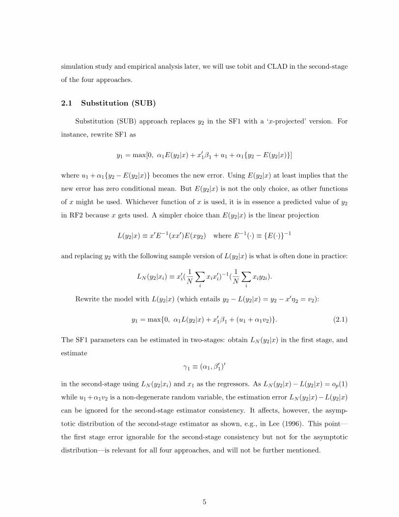
2.1 Substitution (SUB)

Substitution (SUB) approach replaces y2 in the SF1 with a ‘x-projected’ version. For

instance, rewrite SF1 as

y1 = max[0, α1E(y2|x) + x′1β1 + u1 + α1{y2 − E(y2|x)}]

where u1 +α1{y2−E(y2|x)} becomes the new error. Using E(y2|x) at least implies that the

new error has zero conditional mean. But E(y2|x) is not the only choice, as other functions

of x might be used. Whichever function of x is used, it is in essence a predicted value of y2

in RF2 because x gets used. A simpler choice than E(y2|x) is the linear projection

L(y2|x) ≡ x′E−1(xx′)E(xy2) where E−1(·) ≡ {E(·)}−1

and replacing y2 with the following sample version of L(y2|x) is what is often done in practice:

LN (y2|xi) ≡ x′i(1N

∑i

xix′i)−1(

1N

∑i

xiy2i).

Rewrite the model with L(y2|x) (which entails y2 − L(y2|x) = y2 − x′η2 = v2):

y1 = max{0, α1L(y2|x) + x′1β1 + (u1 + α1v2)}. (2.1)

The SF1 parameters can be estimated in two-stages: obtain LN (y2|x) in the first stage, and

estimate

γ1 ≡ (α1, β′1)′

in the second-stage using LN (y2|xi) and x1 as the regressors. As LN (y2|x)−L(y2|x) = op(1)

while u1 +α1v2 is a non-degenerate random variable, the estimation error LN (y2|x)−L(y2|x)

can be ignored for the second-stage estimator consistency. It affects, however, the asymp-

totic distribution of the second-stage estimator as shown, e.g., in Lee (1996). This point—

the first stage error ignorable for the second-stage consistency but not for the asymptotic

distribution—is relevant for all four approaches, and will not be further mentioned.

5

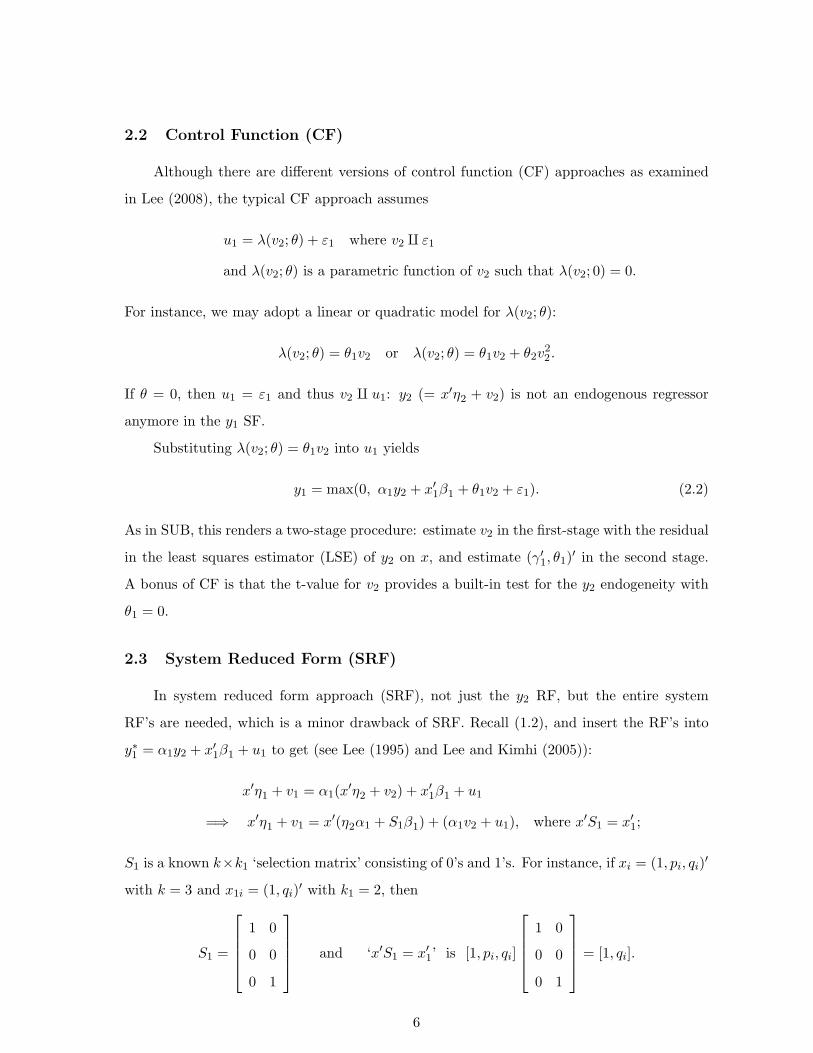
2.2 Control Function (CF)

Although there are different versions of control function (CF) approaches as examined

in Lee (2008), the typical CF approach assumes

u1 = λ(v2; θ) + ε1 where v2 q ε1

and λ(v2; θ) is a parametric function of v2 such that λ(v2; 0) = 0.

For instance, we may adopt a linear or quadratic model for λ(v2; θ):

λ(v2; θ) = θ1v2 or λ(v2; θ) = θ1v2 + θ2v22.

If θ = 0, then u1 = ε1 and thus v2 q u1: y2 (= x′η2 + v2) is not an endogenous regressor

anymore in the y1 SF.

Substituting λ(v2; θ) = θ1v2 into u1 yields

y1 = max(0, α1y2 + x′1β1 + θ1v2 + ε1). (2.2)

As in SUB, this renders a two-stage procedure: estimate v2 in the first-stage with the residual

in the least squares estimator (LSE) of y2 on x, and estimate (γ′1, θ1)′ in the second stage.

A bonus of CF is that the t-value for v2 provides a built-in test for the y2 endogeneity with

θ1 = 0.

2.3 System Reduced Form (SRF)

In system reduced form approach (SRF), not just the y2 RF, but the entire system

RF’s are needed, which is a minor drawback of SRF. Recall (1.2), and insert the RF’s into

y∗1 = α1y2 + x′1β1 + u1 to get (see Lee (1995) and Lee and Kimhi (2005)):

x′η1 + v1 = α1(x′η2 + v2) + x′1β1 + u1

=⇒ x′η1 + v1 = x′(η2α1 + S1β1) + (α1v2 + u1), where x′S1 = x′1;

S1 is a known k×k1 ‘selection matrix’ consisting of 0’s and 1’s. For instance, if xi = (1, pi, qi)′

with k = 3 and x1i = (1, qi)′ with k1 = 2, then

S1 =

1 0

0 0

0 1

and ‘x′S1 = x′1’ is [1, pi, qi]

1 0

0 0

0 1

= [1, qi].

6

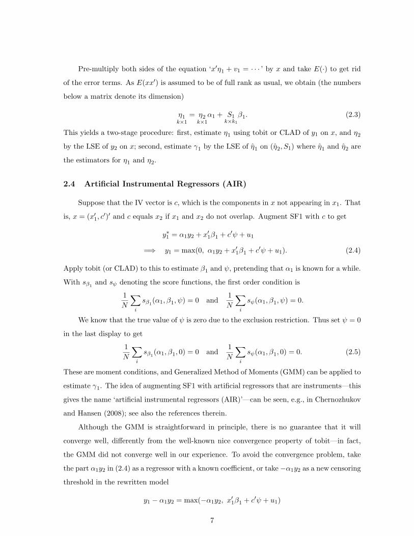
Pre-multiply both sides of the equation ‘x′η1 + v1 = · · · ’ by x and take E(·) to get rid

of the error terms. As E(xx′) is assumed to be of full rank as usual, we obtain (the numbers

below a matrix denote its dimension)

η1k×1

= η2k×1

α1 + S1k×k1

β1. (2.3)

This yields a two-stage procedure: first, estimate η1 using tobit or CLAD of y1 on x, and η2

by the LSE of y2 on x; second, estimate γ1 by the LSE of η̂1 on (η̂2, S1) where η̂1 and η̂2 are

the estimators for η1 and η2.

2.4 Artificial Instrumental Regressors (AIR)

Suppose that the IV vector is c, which is the components in x not appearing in x1. That

is, x = (x′1, c′)′ and c equals x2 if x1 and x2 do not overlap. Augment SF1 with c to get

y∗1 = α1y2 + x′1β1 + c′ψ + u1

=⇒ y1 = max(0, α1y2 + x′1β1 + c′ψ + u1). (2.4)

Apply tobit (or CLAD) to this to estimate β1 and ψ, pretending that α1 is known for a while.

With sβ1and sψ denoting the score functions, the first order condition is

1N

∑i

sβ1(α1, β1, ψ) = 0 and

1N

∑i

sψ(α1, β1, ψ) = 0.

We know that the true value of ψ is zero due to the exclusion restriction. Thus set ψ = 0

in the last display to get

1N

∑i

sβ1(α1, β1, 0) = 0 and

1N

∑i

sψ(α1, β1, 0) = 0. (2.5)

These are moment conditions, and Generalized Method of Moments (GMM) can be applied to

estimate γ1. The idea of augmenting SF1 with artificial regressors that are instruments—this

gives the name ‘artificial instrumental regressors (AIR)’—can be seen, e.g., in Chernozhukov

and Hansen (2008); see also the references therein.

Although the GMM is straightforward in principle, there is no guarantee that it will

converge well, differently from the well-known nice convergence property of tobit—in fact,

the GMM did not converge well in our experience. To avoid the convergence problem, take

the part α1y2 in (2.4) as a regressor with a known coefficient, or take −α1y2 as a new censoring

threshold in the rewritten model

y1 − α1y2 = max(−α1y2, x′1β1 + c′ψ + u1)

7

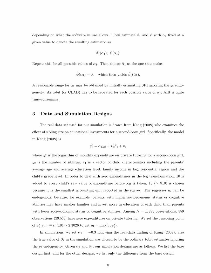
depending on what the software in use allows. Then estimate β1 and ψ with α1 fixed at a

given value to denote the resulting estimator as

β̂1(α1), ψ̂(α1).

Repeat this for all possible values of α1. Then choose α̂1 as the one that makes

ψ̂(α1) = 0, which then yields β̂1(α̂1).

A reasonable range for α1 may be obtained by initially estimating SF1 ignoring the y2 endo-

geneity. As tobit (or CLAD) has to be repeated for each possible value of α1, AIR is quite

time-consuming.

3 Data and Simulation Designs

The real data set used for our simulation is drawn from Kang (2008) who examines the

effect of sibling size on educational investments for a second-born girl. Specifically, the model

in Kang (2008) is

y∗1 = α1y2 + x′1β1 + u1

where y∗1 is the logarithm of monthly expenditure on private tutoring for a second-born girl,

y2 is the number of siblings, x1 is a vector of child characteristics including the parents’

average age and average education level, family income in log, residential region and the

child’s grade level. In order to deal with zero expenditures in the log transformation, 10 is

added to every child’s raw value of expenditure before log is taken; 10 (' $10) is chosen

because it is the smallest accounting unit reported in the survey. The regressor y2 can be

endogenous, because, for example, parents with higher socioeconomic status or cognitive

abilities may have smaller families and invest more in education of each child than parents

with lower socioeconomic status or cognitive abilities. Among N = 1, 893 observations, 559

observations (29.5%) have zero expenditures on private tutoring. We set the censoring point

of y∗1 at τ ≡ ln(10) ' 2.3026 to get y1 = max(τ , y∗1).

In simulations, we set α1 = −0.3 following the real-data finding of Kang (2008); also

the true value of β1 in the simulation was chosen to be the ordinary tobit estimates ignoring

the y2 endogeneity. Given α1 and β1, our simulation designs are as follows. We list the base

design first, and for the other designs, we list only the difference from the base design:

8

• Simulation 0 (Base Design):

1. Generate c, which is an IV for y2, from N(0, 1).

2. Generate v2 from N(0, 1).

3. Given c and v2, generate y2 = 0.3× c+ v2.

4. Given v2, generate u1 = −0.5× v2 + 0.866× ζ where ζ ∼ N(0, 1) so that (u1, v2)

is jointly normal with unit marginal variances and COR(u1, v2) = −0.5.

5. Given y2, u1 and x1 (x1 from the real data), generate y∗1 = −0.3× y2 + x′1β1 + u1,

and finally y1 = max(τ , y∗1).

• Simulation I (Varying Strength of IV): set

Simulation I-1 : y2 = 0.1× c+ v2 in Step 3 (weaker IV)

Simulation I-2 : y2 = 0.6× c+ v2 in Step 3 (stronger IV).

• Simulation II (Dummy Endogenous Regressor y2): in step 3, use y2 = 1[0.3×c+v2 > 0].

• Simulation III (Varying COR(u1, v2)): set

Simulation III-1 : u1 = −0.1× v2 + 0.995× ζ in Step 4

to get COR(u1, v2) = −0.1; (u1, v2) is still jointly normal with unit marginal variances.

Also set

Simulation III-2 : u1 = −0.9× v2 + 0.436× ζ in Step 4

to get COR(u1, v2) = −0.9.

• Simulation IV (Heteroskedastic u1): set

Simulation IV-1 : u1 = −0.5× v2 + πζ · exp(δ1y2 + x′1δ2) in Step 4

where ζ ∼ N(0, 1) and π is a constant to make V (u1) ' 1. For the values of δ1 and δ2,

we use a heteroskedastic tobit estimates with real data:

y1 = max(τ , α1y2 + x′1β1 + ξ1) with V (ξ1|y2, x) = exp(δ1y2 + x′1δ2).

Also we use an heteroskedastic u1 design with δ2 = 0: set

Simulation IV-2 : u1 = −0.5× v2 + πζ · exp(δ1y2) in Step 4.

9

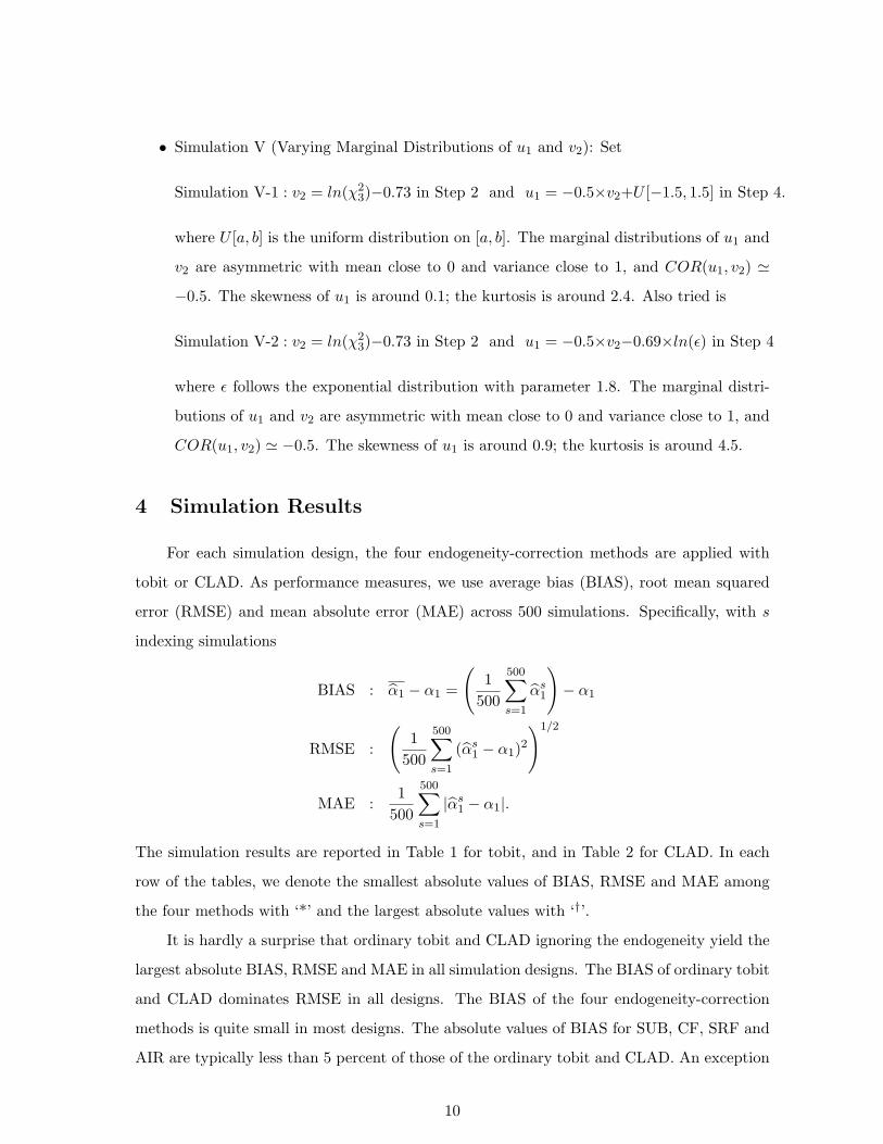
• Simulation V (Varying Marginal Distributions of u1 and v2): Set

Simulation V-1 : v2 = ln(χ23)−0.73 in Step 2 and u1 = −0.5×v2+U [−1.5, 1.5] in Step 4.

where U [a, b] is the uniform distribution on [a, b]. The marginal distributions of u1 and

v2 are asymmetric with mean close to 0 and variance close to 1, and COR(u1, v2) '

−0.5. The skewness of u1 is around 0.1; the kurtosis is around 2.4. Also tried is

Simulation V-2 : v2 = ln(χ23)−0.73 in Step 2 and u1 = −0.5×v2−0.69×ln(ε) in Step 4

where ε follows the exponential distribution with parameter 1.8. The marginal distri-

butions of u1 and v2 are asymmetric with mean close to 0 and variance close to 1, and

COR(u1, v2) ' −0.5. The skewness of u1 is around 0.9; the kurtosis is around 4.5.

4 Simulation Results

For each simulation design, the four endogeneity-correction methods are applied with

tobit or CLAD. As performance measures, we use average bias (BIAS), root mean squared

error (RMSE) and mean absolute error (MAE) across 500 simulations. Specifically, with s

indexing simulations

BIAS : α̂1 − α1 =

(1

500

500∑s=1

α̂s1

)− α1

RMSE :

(1

500

500∑s=1

(α̂s1 − α1)2)1/2

MAE :1

500

500∑s=1

|α̂s1 − α1|.

The simulation results are reported in Table 1 for tobit, and in Table 2 for CLAD. In each

row of the tables, we denote the smallest absolute values of BIAS, RMSE and MAE among

the four methods with ‘*’ and the largest absolute values with ‘†’.

It is hardly a surprise that ordinary tobit and CLAD ignoring the endogeneity yield the

largest absolute BIAS, RMSE and MAE in all simulation designs. The BIAS of ordinary tobit

and CLAD dominates RMSE in all designs. The BIAS of the four endogeneity-correction

methods is quite small in most designs. The absolute values of BIAS for SUB, CF, SRF and

AIR are typically less than 5 percent of those of the ordinary tobit and CLAD. An exception

10

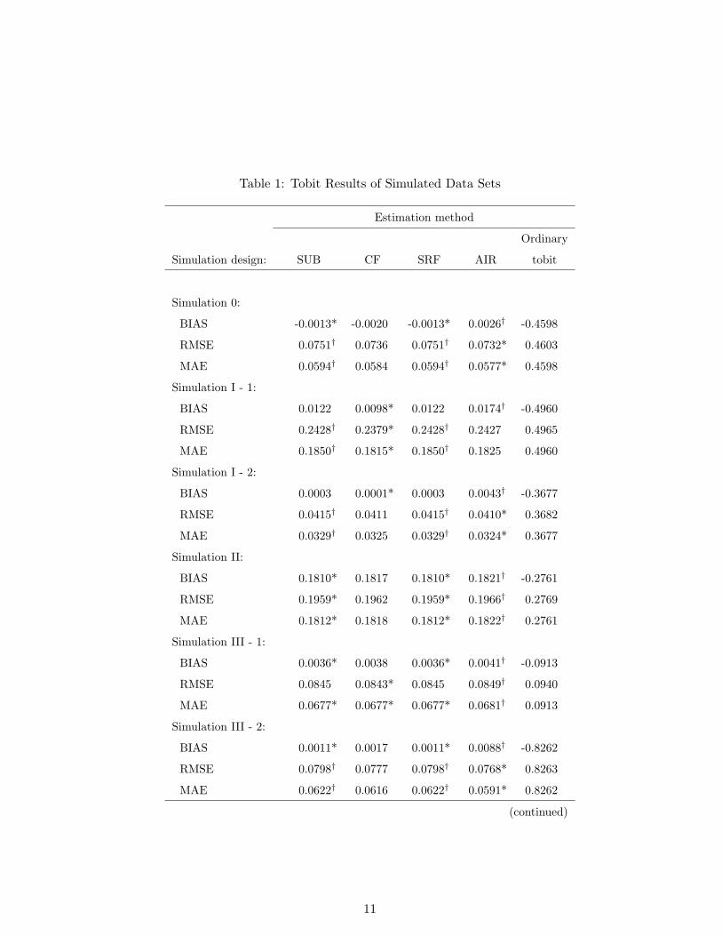
Table 1: Tobit Results of Simulated Data Sets

Estimation method

Ordinary

Simulation design: SUB CF SRF AIR tobit

Simulation 0:

BIAS -0.0013* -0.0020 -0.0013* 0.0026† -0.4598

RMSE 0.0751† 0.0736 0.0751† 0.0732* 0.4603

MAE 0.0594† 0.0584 0.0594† 0.0577* 0.4598

Simulation I - 1:

BIAS 0.0122 0.0098* 0.0122 0.0174† -0.4960

RMSE 0.2428† 0.2379* 0.2428† 0.2427 0.4965

MAE 0.1850† 0.1815* 0.1850† 0.1825 0.4960

Simulation I - 2:

BIAS 0.0003 0.0001* 0.0003 0.0043† -0.3677

RMSE 0.0415† 0.0411 0.0415† 0.0410* 0.3682

MAE 0.0329† 0.0325 0.0329† 0.0324* 0.3677

Simulation II:

BIAS 0.1810* 0.1817 0.1810* 0.1821† -0.2761

RMSE 0.1959* 0.1962 0.1959* 0.1966† 0.2769

MAE 0.1812* 0.1818 0.1812* 0.1822† 0.2761

Simulation III - 1:

BIAS 0.0036* 0.0038 0.0036* 0.0041† -0.0913

RMSE 0.0845 0.0843* 0.0845 0.0849† 0.0940

MAE 0.0677* 0.0677* 0.0677* 0.0681† 0.0913

Simulation III - 2:

BIAS 0.0011* 0.0017 0.0011* 0.0088† -0.8262

RMSE 0.0798† 0.0777 0.0798† 0.0768* 0.8263

MAE 0.0622† 0.0616 0.0622† 0.0591* 0.8262

(continued)

11

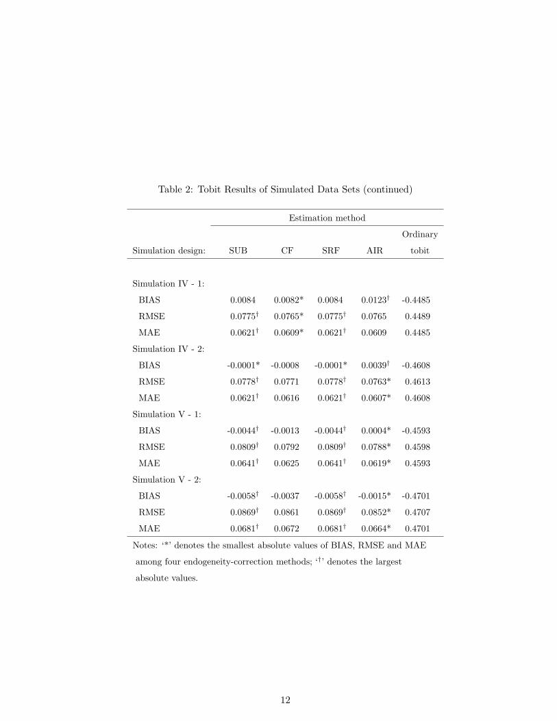
Table 2: Tobit Results of Simulated Data Sets (continued)

Estimation method

Ordinary

Simulation design: SUB CF SRF AIR tobit

Simulation IV - 1:

BIAS 0.0084 0.0082* 0.0084 0.0123† -0.4485

RMSE 0.0775† 0.0765* 0.0775† 0.0765 0.4489

MAE 0.0621† 0.0609* 0.0621† 0.0609 0.4485

Simulation IV - 2:

BIAS -0.0001* -0.0008 -0.0001* 0.0039† -0.4608

RMSE 0.0778† 0.0771 0.0778† 0.0763* 0.4613

MAE 0.0621† 0.0616 0.0621† 0.0607* 0.4608

Simulation V - 1:

BIAS -0.0044† -0.0013 -0.0044† 0.0004* -0.4593

RMSE 0.0809† 0.0792 0.0809† 0.0788* 0.4598

MAE 0.0641† 0.0625 0.0641† 0.0619* 0.4593

Simulation V - 2:

BIAS -0.0058† -0.0037 -0.0058† -0.0015* -0.4701

RMSE 0.0869† 0.0861 0.0869† 0.0852* 0.4707

MAE 0.0681† 0.0672 0.0681† 0.0664* 0.4701

Notes: ‘*’ denotes the smallest absolute values of BIAS, RMSE and MAE

among four endogeneity-correction methods; ‘†’ denotes the largest

absolute values.

12

Table 3: CLAD Results of Simulated Data Sets

Estimation method

Ordinary

Simulation design: SUB CF SRF AIR CLAD

Simulation 0:

BIAS 0.0011* -0.0019 0.0014 0.0038† -0.4593

RMSE 0.1062† 0.0933 0.1059 0.0800* 0.4602

MAE 0.0841† 0.0735 0.0837 0.0628* 0.4593

Simulation I - 1:

BIAS 0.0177† 0.0094* 0.0177† 0.0100 -0.4954

RMSE 0.3381 0.3081 0.3394† 0.2414* 0.4962

MAE 0.2654 0.2329 0.2666† 0.1841* 0.4954

Simulation I - 2:

BIAS 0.0022 0.0001* 0.0022 0.0074† -0.3669

RMSE 0.0541 0.0497 0.0543† 0.0472* 0.3677

MAE 0.0432 0.0397 0.0434† 0.0376* 0.3669

Simulation II:

BIAS 0.1611* 0.1799† 0.1611* 0.1766 -0.2781

RMSE 0.1893* 0.2020† 0.1894 0.1928 0.2795

MAE 0.1656* 0.1827† 0.1656 0.1771 0.2781

Simulation III - 1:

BIAS 0.0055 0.0062† 0.0058 0.0048* -0.0907

RMSE 0.1017 0.1018† 0.1013 0.0874* 0.0949

MAE 0.0799 0.0802† 0.0796 0.0685* 0.0907

Simulation III - 2:

BIAS 0.0071 0.0002* 0.0067 0.0117† -0.8259

RMSE 0.1090 0.0816* 0.1090† 0.0827 0.8261

MAE 0.0851 0.0632* 0.0853† 0.0643 0.8259

(continued)

13

Table 4: CLAD Results of Simulated Data Sets (continued)

Estimation method

Ordinary

Simulation design: SUB CF SRF AIR CLAD

Simulation IV - 1:

BIAS 0.0074 0.0063* 0.0071 0.0110† -0.4575

RMSE 0.1020† 0.0890 0.1015 0.0813* 0.4581

MAE 0.0821† 0.0720 0.0817 0.0644* 0.4575

Simulation IV - 2:

BIAS -0.0026 -0.0015* -0.0027 0.0053† -0.4606

RMSE 0.1091† 0.0985 0.1090 0.0837* 0.4613

MAE 0.0851† 0.0795 0.0847 0.0670* 0.4606

Simulation V - 1:

BIAS -0.0049 -0.0061† -0.0047 -0.0021* -0.4597

RMSE 0.1190 0.1284† 0.1190 0.0958* 0.4611

MAE 0.0950 0.1017† 0.0951 0.0766* 0.4597

Simulation V - 2:

BIAS 0.0024 0.0009* 0.0026 0.0032† -0.4606

RMSE 0.1079 0.0874* 0.1082† 0.0893 0.4612

MAE 0.0850 0.0695* 0.0855† 0.0720 0.4606

Notes: ‘*’ denotes the smallest absolute values of BIAS, RMSE and MAE

among four endogeneity-correction methods; ‘†’ denotes the largest

absolute values.

14

is simulation II in which a dummy y2 is used instead of a continuous y2; in this design, the

absolute BIAS for all endogeneity-correction methods is around 60 percent of that of the

ordinary tobit and CLAD. Also, in simulation II, BIAS accounts for more than 70 percent of

RMSE. This suggests that caution is required when y2 is a dummy rather than a continuous

variable and a dummy y2 seems to need a further study.

Among the four endogeneity-correction methods, AIR performs worst in terms of BIAS.

AIR yields the largest absolute BIAS in 8 (6) out of 10 simulation designs for tobit (CLAD).

In contrast, CF appears to perform best among the four methods. Although it produces the

largest absolute BIAS with CLAD estimates in 3 designs, CF yields the smallest absolute

BIAS in 3 and 6 designs when tobit and CLAD are applied, respectively. SUB and SRF show

intermediate levels of performance for tobit and CLAD.

While AIR performs relatively poorly in BIAS, it performs best for both tobit and CLAD

in terms of RMSE and MAE. For a majority of the cases—6 designs in tobit and 7 designs

in CLAD, AIR yields the smallest RMSE and MAE. In contrast, SUB and SRF perform

worst for tobit in terms of RMSE and MAE with the largest RMSE and MAE in 8 designs,

but perform comparably to CF for CLAD. SUB and SRF returned the same estimates for

tobit, but different ones for CLAD; SUB does somewhat better than SRF for CLAD. In some

models, equivalences of certain estimators can be established under some assumptions—e.g.,

for linear models, Lee (2008) shows SUB=AIR—Table 1 suggests SUB=SRF for tobit, but

proving this goes beyond the scope of this paper.

To summarize, in terms of BIAS, CF seems to perform best and AIR performs worst

among the four endogeneity-correction methods. In terms of RMSE and MAE, however,

AIR performs best, and SUB and SRF performs worst. Because RMSE and MAE are in

general regarded as more comprehensive performance measures than BIAS, these findings

favor AIR over the other methods. But AIR takes hundreds times longer than the others in

computation because a grid search is required for each possible value of α1. Also CF requires

most restrictive assumptions. Hence the choice of an estimator seems case-specific. This

conclusion notwithstanding, it should be noted that the performance differences were fairly

small across the four approaches in our simulation designs.

15

5 Empirical Analysis

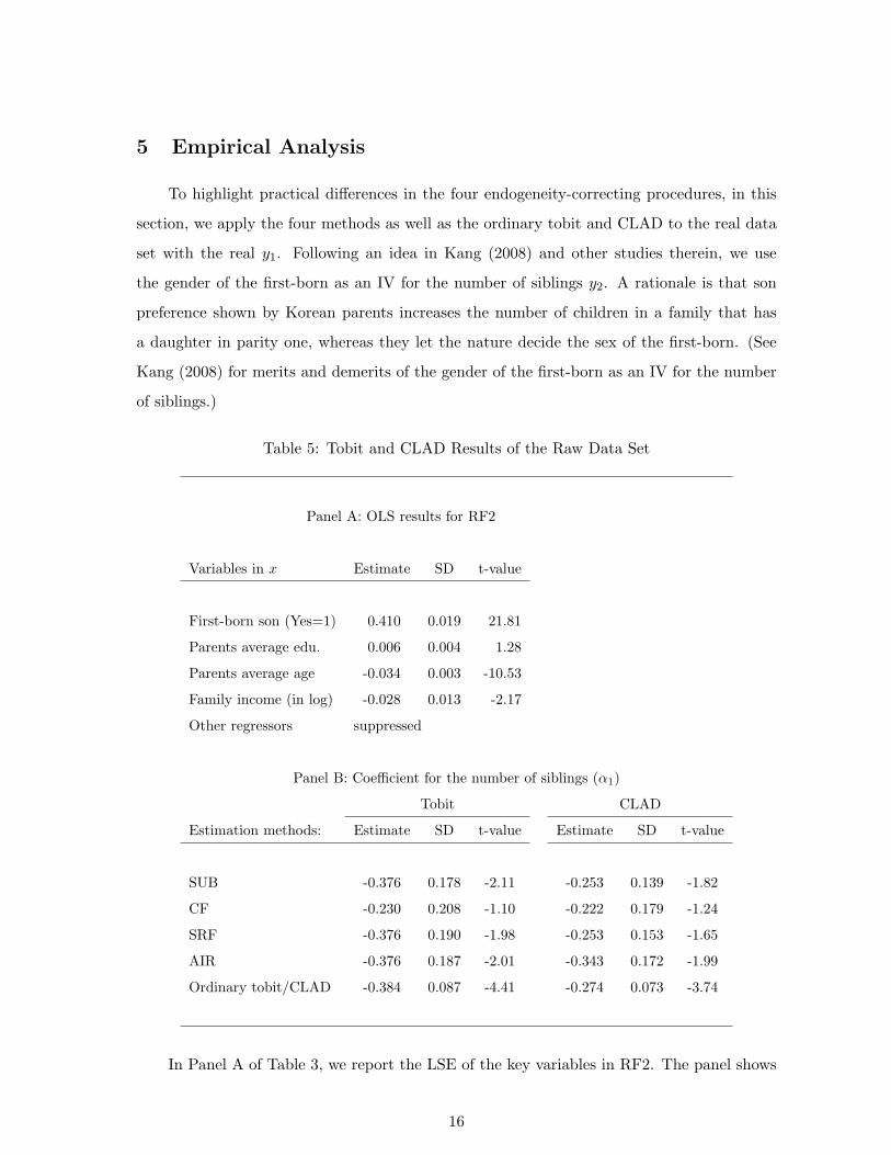
To highlight practical differences in the four endogeneity-correcting procedures, in this

section, we apply the four methods as well as the ordinary tobit and CLAD to the real data

set with the real y1. Following an idea in Kang (2008) and other studies therein, we use

the gender of the first-born as an IV for the number of siblings y2. A rationale is that son

preference shown by Korean parents increases the number of children in a family that has

a daughter in parity one, whereas they let the nature decide the sex of the first-born. (See

Kang (2008) for merits and demerits of the gender of the first-born as an IV for the number

of siblings.)

Table 5: Tobit and CLAD Results of the Raw Data Set

Panel A: OLS results for RF2

Variables in x Estimate SD t-value

First-born son (Yes=1) 0.410 0.019 21.81

Parents average edu. 0.006 0.004 1.28

Parents average age -0.034 0.003 -10.53

Family income (in log) -0.028 0.013 -2.17

Other regressors suppressed

Panel B: Coefficient for the number of siblings (α1)

Tobit CLAD

Estimation methods: Estimate SD t-value Estimate SD t-value

SUB -0.376 0.178 -2.11 -0.253 0.139 -1.82

CF -0.230 0.208 -1.10 -0.222 0.179 -1.24

SRF -0.376 0.190 -1.98 -0.253 0.153 -1.65

AIR -0.376 0.187 -2.01 -0.343 0.172 -1.99

Ordinary tobit/CLAD -0.384 0.087 -4.41 -0.274 0.073 -3.74

In Panel A of Table 3, we report the LSE of the key variables in RF2. The panel shows

16

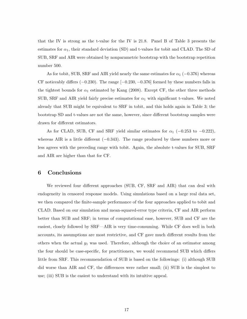
that the IV is strong as the t-value for the IV is 21.8. Panel B of Table 3 presents the

estimates for α1, their standard deviation (SD) and t-values for tobit and CLAD. The SD of

SUB, SRF and AIR were obtained by nonparametric bootstrap with the bootstrap repetition

number 500.

As for tobit, SUB, SRF and AIR yield nearly the same estimates for α1 (−0.376) whereas

CF noticeably differs (−0.230). The range [−0.230,−0.376] formed by these numbers falls in

the tightest bounds for α1 estimated by Kang (2008). Except CF, the other three methods

SUB, SRF and AIR yield fairly precise estimates for α1 with significant t-values. We noted

already that SUB might be equivalent to SRF in tobit, and this holds again in Table 3; the

bootstrap SD and t-values are not the same, however, since different bootstrap samples were

drawn for different estimators.

As for CLAD, SUB, CF and SRF yield similar estimates for α1 (−0.253 to −0.222),

whereas AIR is a little different (−0.343). The range produced by these numbers more or

less agrees with the preceding range with tobit. Again, the absolute t-values for SUB, SRF

and AIR are higher than that for CF.

6 Conclusions

We reviewed four different approaches (SUB, CF, SRF and AIR) that can deal with

endogeneity in censored response models. Using simulations based on a large real data set,

we then compared the finite-sample performance of the four approaches applied to tobit and

CLAD. Based on our simulation and mean-squared-error type criteria, CF and AIR perform

better than SUB and SRF; in terms of computational ease, however, SUB and CF are the

easiest, closely followed by SRF—AIR is very time-consuming. While CF does well in both

accounts, its assumptions are most restrictive, and CF gave much different results from the

others when the actual y1 was used. Therefore, although the choice of an estimator among

the four should be case-specific, for practitioners, we would recommend SUB which differs

little from SRF. This recommendation of SUB is based on the followings: (i) although SUB

did worse than AIR and CF, the differences were rather small; (ii) SUB is the simplest to

use; (iii) SUB is the easiest to understand with its intuitive appeal.

17

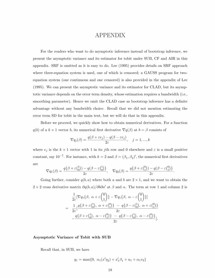
APPENDIX

For the readers who want to do asymptotic inference instead of bootstrap inference, we

present the asymptotic variance and its estimator for tobit under SUB, CF and AIR in this

appendix. SRF is omitted as it is easy to do. Lee (1995) provides details on SRF approach

where three-equation system is used, one of which is censored; a GAUSS program for two-

equation system (one continuous and one censored) is also provided in the appendix of Lee

(1995). We can present the asymptotic variance and its estimator for CLAD, but its asymp-

totic variance depends on the error term density, whose estimation requires a bandwidth (i.e.,

smoothing parameter). Hence we omit the CLAD case as bootstrap inference has a definite

advantage without any bandwidth choice. Recall that we did not mention estimating the

error term SD for tobit in the main text, but we will do that in this appendix.

Before we proceed, we quickly show how to obtain numerical derivatives. For a function

q(b) of a k × 1 vector b, its numerical first derivative ∇q(β) at b = β consists of

∇qj(β) =q(β + εej)− q(β − εej)

2ε, j = 1, ..., k

where ej is the k × 1 vector with 1 in its jth row and 0 elsewhere and ε is a small positive

constant, say 10−7. For instance, with k = 2 and β = (β1, β2)′, the numerical first derivatives

are

∇q1(β) =q{β + ε

(10

))− q(β − ε

(10

)}

2ε, ∇q2(β) =

q{β + ε(01

))− q(β − ε

(01

)}

2ε.

Going further, consider q(b, a) where both a and b are 2× 1, and we want to obtain the

2× 2 cross derivative matrix ∂q(b, a)/∂b∂a′ at β and α. The term at row 1 and column 2 is

12ε

[∇q1{β, α+ ε

(01

)} − ∇q1{β, α− ε

(01

)}]

=12ε

[q{β + ε

(10

), α+ ε

(01

)} − q{β − ε

(10

), α+ ε

(01

)}

2ε

−q{β + ε

(10

), α− ε

(01

)} − q{β − ε

(10

), α− ε

(01

)}

2ε].

Asymptotic Variance of Tobit with SUB

Recall that, in SUB, we have

y1 = max{0, α1(x′η2) + x′1β1 + u1 + α1v2}

18

where η2 is the first-stage parameter estimated by the LSE of y2 on x. To make estimating

the error term SD explicit, redefine γ1 as

γ1 ≡ (α1, β′1, σ12)′ where σ12 ≡ SD(u1 + α1v2).

Let sγ1(γ̂1, η̂2) be the (k1 +2)×1 tobit score function for γ1 using (x′η̂2, x

′1) as the regressors

evaluated at γ̂1 and η̂2, where γ̂1 is the tobit and η̂2 is the LSE for η2. Clearly, random

variables are included in sγ1, which are omitted to simplify the presentation.

The following asymptotic expansion holds (see, e.g., Lee (1996, 2009)): omitting the

arguments in sγ1(γ1, η2) when the arguments are the true values,

√N(γ̂1 − γ1) = −E−1(sγ1

sγ′1) · { 1√

N

∑i

sγ1+ E(

∂sγ1

∂η′2)√N(η̂2 − η2)}+ op(1)

= −E−1(sγ1sγ′

1) · 1√

N

∑i

{sγ1+ E(

∂sγ1

∂η′2)ζi}+ op(1) because

√N(η̂2 − η2) =

1√N

∑i

ζi + op(1) where ζi = E−1(xx′) · xiv2i.

Hence, with ‘ ’ denoting convergence in law,

√N(γ̂1 − γ1) N{0, E−1(sγ1

sγ′1) · Cγ1

· E−1(sγ1sγ′

1)} where

Cγ1≡ E[{sγ1

+ E(∂sγ1

∂η′2)ζ}{sγ1

+ E(∂sγ1

∂η′2)ζ}′].

As for estimating the asymptotic variance,

1N

∑i

sγ1(γ̂1, η̂2)sγ1

(γ̂1, η̂2)′ →p E(sγ1sγ′

1) and

1N

∑i

δ̂iδ̂′i →p Cγ1

where

δ̂i ≡ sγ1(γ̂1, η̂2) + { 1

N

∑i

∂sγ1(γ̂1, η̂2)∂η′2

}( 1N

∑i

xix′i)−1xi(y2i − x′iη̂2).

The (k1 + 2) × k derivative matrix ∂sγ1/∂η′2 can be found by numerical gradients; deriving

its analytical form will be rather involved.

Asymptotic Variance of Tobit with CF

In CF, we have u1 = θ1v2 + ε1 with v2 q ε1, and thus

y1 = max{0, α1y2 + x′1β1 + θ1(y2 − x′η2) + ε1}.

Let

µ1 ≡ (α1, β′1, θ1, σε)′ where σε ≡ SD(ε1)

19

and sµ1(µ̂1, η̂2) be the (k1 + 3) × 1 score function for µ1 using (y2, x

′1, v̂2) as the regressors,

where µ̂1 is the tobit and v̂2 ≡ y2 − x′η̂2; η2 is still the first-stage parameter.

Analogously to the SUB case, the following asymptotic expansion holds:

√N(µ̂1 − µ1) = −E−1(sµ1

sµ′1) · 1√

N

∑i

{sµ1+ E(

∂sµ1

∂η′2)ζi}+ op(1).

Hence

√N(µ̂1 − µ1) N{0, E−1(sµ1

sµ′1) · Cµ1

· E−1(sµ1sµ′

1)} where

Cµ1≡ E[{sµ1

+ E(∂sµ1

∂η′2)ζ}{sµ1

+ E(∂sµ1

∂η′2)ζ}′].

As for estimating the asymptotic variance,

1N

∑i

sµ1(µ̂1, η̂2)sµ1

(µ̂1, η̂2)′ →p E(sµ1sµ′

1) and

1N

∑i

δ̃iδ̃′i →p Cµ1

where

δ̃i ≡ sµ1(µ̂1, η̂2) + { 1

N

∑i

∂sµ1(µ̂1, η̂2)∂η′2

}( 1N

∑i

xix′i)−1xiv̂2i.

Asymptotic Variance of Tobit with AIR

For AIR, denote the tobit score function for (β′1, σ1, ψ′)′ with σ1 ≡ SD(u1) as

s−α(α1, β1, σ1, ψ) = s−α(γ1, ψ) where γ1 ≡ (α1, β′1, σ1)′;

although we use the same notation γ1, γ1 here differs from the above γ1 for SUB, because

the error term SD’s are different. Recalling (2.5), the AIR estimator γ̂1 satisfies the moment

condition1N

∑i

s−α(γ̂1, 0) = 0.

Consider the “just-identified” case where ψ is a scalar so that the dimension of (β′1, σ1, ψ′)′

is the same as that of γ1. Taylor-expand the last display around γ1 to get

0 =1√N

∑i

s−α(γ1, 0) +1N

∑i

∂s−α(γ1, 0)∂γ′1

√N(γ̂1 − γ1) + op(1)

=⇒√N(γ̂1 − γ1) = { 1

N

∑i

∂s−α(γ1, 0)∂γ′1

}−1 −1√N

∑i

s−α(γ1, 0) + op(1)

N [0, E−1{∂s−α(γ1, 0)∂γ′1

}E{s−α(γ1, 0)s−α(γ1, 0)′}E−1{∂s−α(γ1, 0)∂γ1

}].

20

As for estimating the asymptotic variance,

1N

∑i

∂s−α(γ̂1, 0)∂γ1

→p E{∂s−α(γ1, 0)∂γ1

}

1N

∑i

s−α(γ̂1, 0)s−α(γ̂1, 0)′ →p E{s−α(γ1, 0)s−α(γ1, 0)′}.

In the “over-identified” case, i.e., when ψ is not a scalar, E{∂s−α(γ1, 0)/∂γ1} is not

square, and thus not invertible. In this case, it is possible to proceed as in GMM over-

identified case using the above moment condition. But this case raises the issue of which

function of c to use; e.g., not just c, its polynomial functions can be used as well. This

aspect is a shortcoming of AIR. Instead of mulling over what to do, it is much simpler in

practice to turn the instrument vector c into a single variable, and one good choice would

be using LN (y2|c), following the usual practice of two-stage LSE. Using LN (y2|c) instead of

L(y2|c) does not affect the asymptotic distribution of AIR, following the fact that estimating

instruments is innocuous (whereas estimating regressors is not); see Lee (1996,2009). In the

moment condition with ψ = 0, LN (y2|c) appears only as an instrument.

21

REFERENCES

Angrist, J.D., 2001, Estimation of limited dependent variable models with dummy en-

dogenous regressors: simple strategies for empirical practice, Journal of Business and Eco-

nomic Statistics 19, 2-16.

Blundell, R.W. and J.L. Powell, 2003, Endogeneity in nonparametric and semiparametric

regression models, Advances in Economics and Econometrics: Theory and Applications,

Eighth World Congress, Vol.II, edited by M. Dewatripont, L.P. Hansen, and S.J. Turnovsky,

Cambridge University Press.

Blundell, R.W. and J.L. Powell, 2004, Endogeneity in semiparametric binary response

models, Review of Economic Studies 71, 655-679.

Blundell, R.W. and R.J. Smith, 1986, An exogeneity test for a simultaneous equation

tobit model with an application to labor supply, Econometrica 54, 679-685.

Blundell, R.W. and R.J. Smith, 1993, Simultaneous microeconometric models with cen-

sored or qualitative dependent variables, in Handbook of Statistics 11, edited by G.S. Mad-

dala, C.R. Rao and H.D. Vinod, North Holland.

Chernozhukov, V. and C. Hansen, 2008, Instrumental variable quantile regression: a

robust inference approach, Journal of Econometrics 142, 379–398.

Kang, C., 2008, Family size and educational investments in children: evidence from

private tutoring expenditures in South Korea, unpublished paper.

Kerkhofs, M., M. Lindeboom and J. Theeuwes, 1999, Retirement, financial incentives

and health, Labour Economics 6, 203-227.

Labeaga, J.M., 1999, A double-hurdle rational addiction model with heterogeneity: es-

timating the demand for tobacco, Journal of Econometrics 93, 49-72.

Lee, M.J., 1992, Winsorized mean estimator for censored regression, Econometric Theory

8, 368-382.

Lee, M.J., 1995, Semiparametric estimation of simultaneous equations with limited de-

pendent variables: a case study of female labor supply, Journal of Applied Econometrics 10,

187-200.

Lee, M.J., 1996, Nonparametric two stage estimation of simultaneous equations with

limited endogenous regressors, Econometric Theory 12, 305-330.

22

Lee, M.J., 2008, Semiparametric estimators for limited dependent variable (LDV) models

with endogenous regressors, unpublished paper.

Lee, M.J., 2009, Micro-econometrics: methods of moments and limited dependent vari-

ables, Springer, forthcoming.

Lee, M.J. and A. Kimhi, 2005, Simultaneous equations in ordered discrete responses with

regressor-dependent thresholds, Econometrics Journal 8, 176-196.

Lewbel, A., 2007, Coherency and completeness of structural models containing a dummy

endogenous variable, International Economic Review 48, 1379-1392.

Pagan, A.R. and A. Ullah, 1999, Nonparametric econometrics, Cambridge University

Press.

Powell, J.L., 1984, Least absolute deviations estimation for the censored regression

model, Journal of Econometrics 25, 303-325.

Powell, J.L., 1986a, Symmetrically trimmed least squares estimation for Tobit models,

Econometrica 54, 1435-1460.

Powell, J.L., 1986b, Censored regression quantiles, Journal of Econometrics 32, 143-155.

Powell, J.L., 1994, Estimation of semiparametric models, in Handbook of Econometrics

IV, edited by R.F. Engle and D.L. McFadden, Elsevier.

Savage, E. and D.J. Wright, 2003, Moral hazard and adverse selection in Australian

private hospitals: 1989–1990, Journal of Health Economics 22, 331–359.

23