Embed Size (px)
Citation preview
Eur. Phys. J. C (2017) 77:317DOI 10.1140/epjc/s10052-017-4852-3
Regular Article - Experimental Physics
Performance of the ATLAS trigger system in 2015
ATLAS Collaboration�
CERN, 1211 Geneva 23, Switzerland
Received: 30 November 2016 / Accepted: 23 April 2017 / Published online: 18 May 2017© CERN for the benefit of the ATLAS collaboration 2017. This article is an open access publication
Abstract During 2015 the ATLAS experiment recorded3.8 fb−1 of proton–proton collision data at a centre-of-massenergy of 13 TeV. The ATLAS trigger system is a cru-cial component of the experiment, responsible for selectingevents of interest at a recording rate of approximately 1 kHzfrom up to 40 MHz of collisions. This paper presents a shortoverview of the changes to the trigger and data acquisitionsystems during the first long shutdown of the LHC and showsthe performance of the trigger system and its componentsbased on the 2015 proton–proton collision data.
Contents
1 Introduction . . . . . . . . . . . . . . . . . . . . . 22 ATLAS detector . . . . . . . . . . . . . . . . . . . 23 Changes to the Trigger/DAQ system for Run 2 . . . 3
3.1 Level-1 calorimeter trigger . . . . . . . . . . . 43.2 Level-1 muon trigger . . . . . . . . . . . . . . 5
4 Trigger menu . . . . . . . . . . . . . . . . . . . . . 64.1 Physics trigger menu for 2015 data-taking . . . 74.2 Event streaming . . . . . . . . . . . . . . . . . 84.3 HLT processing time . . . . . . . . . . . . . . 94.4 Trigger menu for special data-taking conditions 9
5 High-level trigger reconstruction . . . . . . . . . . 105.1 Inner detector tracking . . . . . . . . . . . . . 11
5.1.1 Inner detector tracking algorithms . . . . 115.1.2 Inner detector tracking performance . . . 115.1.3 Multiple stage tracking . . . . . . . . . . 115.1.4 Inner detector tracking timing . . . . . . 14
5.2 Calorimeter reconstruction . . . . . . . . . . . 145.2.1 Calorimeter algorithms . . . . . . . . . . 145.2.2 Calorimeter algorithm performance . . . 155.2.3 Calorimeter algorithm timing . . . . . . . 16
5.3 Tracking in the muon spectrometer . . . . . . . 165.3.1 Muon tracking algorithms . . . . . . . . 165.3.2 Muon tracking performance . . . . . . . 175.3.3 Muon tracking timing . . . . . . . . . . . 17
� e-mail: [email protected]
6 Trigger signature performance . . . . . . . . . . . . 18
6.1 Minimum-bias and forward triggers . . . . . . 18
6.1.1 Reconstruction and selection . . . . . . . 18
6.1.2 Trigger efficiencies . . . . . . . . . . . . 19
6.2 Electrons and photons . . . . . . . . . . . . . . 20
6.2.1 Electron and photon reconstruction andselection . . . . . . . . . . . . . . . . . 20
6.2.2 Electron and photon trigger menu and rates 21
6.2.3 Electron and photon trigger efficiencies . 21
6.3 Muons . . . . . . . . . . . . . . . . . . . . . . 22
6.3.1 Muon reconstruction and selection . . . . 23
6.3.2 Muon trigger menu and rates . . . . . . . 23
6.3.3 Muon trigger efficiencies . . . . . . . . . 23
6.4 Jets . . . . . . . . . . . . . . . . . . . . . . . . 24
6.4.1 Jet reconstruction . . . . . . . . . . . . . 25
6.4.2 Jet trigger menu and rates . . . . . . . . 25
6.4.3 Jet trigger efficiencies . . . . . . . . . . 25
6.4.4 Jets and trigger-level analysis . . . . . . . 27
6.5 Tau leptons . . . . . . . . . . . . . . . . . . . 27
6.5.1 Tau reconstruction and selection . . . . . 28
6.5.2 Tau trigger menu and rates . . . . . . . . 28
6.5.3 Tau trigger efficiencies . . . . . . . . . . 28
6.6 Missing transverse momentum . . . . . . . . . 29
6.6.1 EmissT reconstruction and selection . . . . 29
6.6.2 EmissT trigger menu and rates . . . . . . . 32
6.6.3 EmissT trigger efficiencies . . . . . . . . . 32
6.7 b-Jets . . . . . . . . . . . . . . . . . . . . . . 34
6.7.1 b-Jet reconstruction and selection . . . . 35
6.7.2 b-Jet trigger menu and rates . . . . . . . 36
6.8 B-physics . . . . . . . . . . . . . . . . . . . . 37
6.8.1 B-physics reconstruction and selection . . 37
6.8.2 B-physics trigger menu and rates . . . . . 37
6.8.3 B-physics trigger efficiencies . . . . . . . 38
7 Conclusion . . . . . . . . . . . . . . . . . . . . . . 38
References . . . . . . . . . . . . . . . . . . . . . . . . 39
123

317 Page 2 of 53 Eur. Phys. J. C (2017) 77 :317
1 Introduction
The trigger system is an essential component of any colliderexperiment as it is responsible for deciding whether or notto keep an event from a given bunch-crossing interactionfor later study. During Run 1 (2009 to early 2013) of theLarge Hadron Collider (LHC), the trigger system [1–5] of theATLAS experiment [6] operated efficiently at instantaneousluminosities of up to 8 × 1033 cm−2 s−1 and primarily atcentre-of-mass energies,
√s, of 7 TeV and 8 TeV. In Run 2
(since 2015) the increased centre-of-mass energy of 13 TeV,higher luminosity and increased number of proton–protoninteractions per bunch-crossing (pile-up) meant that, withoutupgrades of the trigger system, the trigger rates would haveexceeded the maximum allowed rates when running with thetrigger thresholds needed to satisfy the physics programmeof the experiment. For this reason, the first long shutdown(LS1) between LHC Run 1 and Run 2 operations was usedto improve the trigger system with almost no component leftuntouched.
After a brief introduction of the ATLAS detector in Sect. 2,Sect. 3 summarises the changes to the trigger and data acqui-sition during LS1. Section 4 gives an overview of the triggermenu used during 2015 followed by an introduction to thereconstruction algorithms used at the high-level trigger inSect. 5. The performance of the different trigger signaturesis shown in Sect. 6 for the data taken with 25 ns bunch-spacing in 2015 at a peak luminosity of 5 × 1033 cm−2 s−1
with comparison to Monte Carlo (MC) simulation.
2 ATLAS detector
ATLAS is a general-purpose detector with a forward-backward symmetry, which provides almost full solid anglecoverage around the interaction point.1 The main compo-nents of ATLAS are an inner detector (ID), which is sur-rounded by a superconducting solenoid providing a 2T axialmagnetic field, a calorimeter system, and a muon spectrom-eter (MS) in a magnetic field generated by three large super-conducting toroids with eight coils each. The ID providestrack reconstruction within |η| < 2.5, employing a pixeldetector (Pixel) close to the beam pipe, a silicon microstripdetector (SCT) at intermediate radii, and a transition radi-ation tracker (TRT) at outer radii. A new innermost pixel-detector layer, the insertable B-layer (IBL), was added dur-
1 ATLAS uses a right-handed coordinate system with its origin at thenominal interaction point (IP) in the centre of the detector and the z-axisalong the beam pipe. The x-axis points from the IP to the centre of theLHC ring, and the y-axis points upward. Cylindrical coordinates (r, φ)
are used in the transverse plane, φ being the azimuthal angle around thez-axis. The pseudorapidity is defined in terms of the polar angle θ asη = − ln tan(θ/2).
ing LS1 at a radius of 33 mm around a new and thinnerbeam pipe [7]. The calorimeter system covers the region|η| < 4.9, the forward region (3.2 < |η| < 4.9) being instru-mented with a liquid-argon (LAr) calorimeter for electro-magnetic and hadronic measurements. In the central region,a lead/LAr electromagnetic calorimeter covers |η| < 3.2,while the hadronic calorimeter uses two different detec-tor technologies, with steel/scintillator tiles (|η| < 1.7) orlead/LAr (1.5 < |η| < 3.2) as absorber/active material. TheMS consists of one barrel (|η| < 1.05) and two end-cap sec-tions (1.05 < |η| < 2.7). Resistive plate chambers (RPC,three doublet layers for |η| < 1.05) and thin gap cham-bers (TGC, one triplet layer followed by two doublets for1.0 < |η| < 2.4) provide triggering capability as well as(η, φ) position measurements. A precise momentum mea-surement for muons with |η| up to 2.7 is provided by threelayers of monitored drift tubes (MDT), with each chamberproviding six to eight η measurements along the muon tra-jectory. For |η| > 2, the inner layer is instrumented withcathode strip chambers (CSC), consisting of four sensitivelayers each, instead of MDTs.
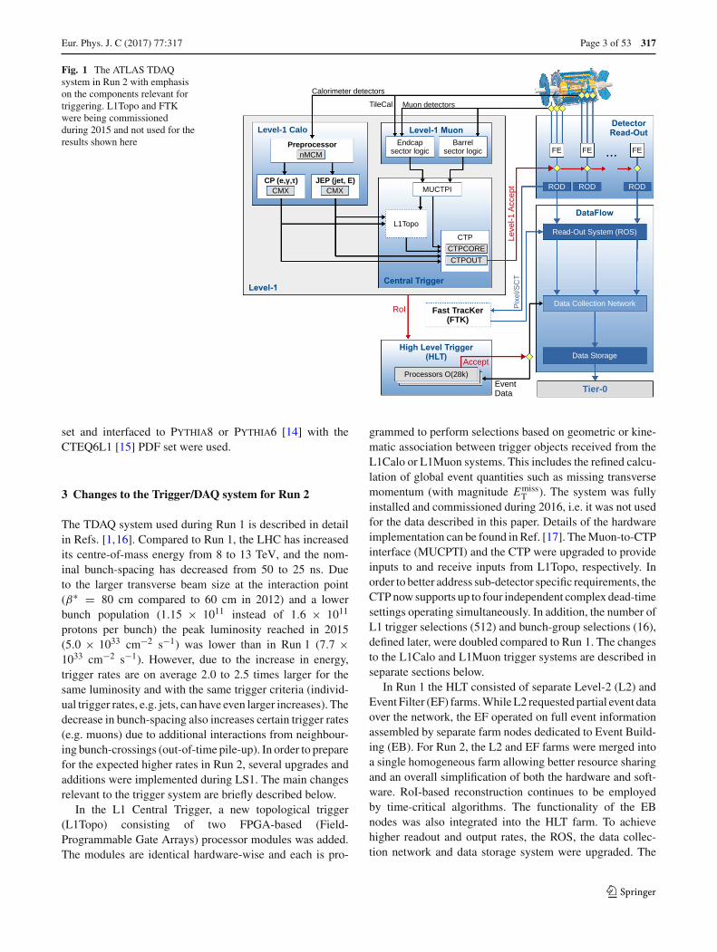
The Trigger and Data Acquisition (TDAQ) system shownin Fig. 1 consists of a hardware-based first-level trigger(L1) and a software-based high-level trigger (HLT). The L1trigger decision is formed by the Central Trigger Proces-sor (CTP), which receives inputs from the L1 calorimeter(L1Calo) and L1 muon (L1Muon) triggers as well as severalother subsystems such as the Minimum Bias Trigger Scintil-lators (MBTS), the LUCID Cherenkov counter and the Zero-Degree Calorimeter (ZDC). The CTP is also responsible forapplying preventive dead-time. It limits the minimum timebetween two consecutive L1 accepts (simple dead-time) toavoid overlapping readout windows, and restricts the numberof L1 accepts allowed in a given number of bunch-crossings(complex dead-time) to avoid front-end buffers from over-flowing. In 2015 running, the simple dead-time was set to4 bunch-crossings (100 ns). A more detailed description ofthe L1 trigger system can be found in Ref. [1]. After the L1trigger acceptance, the events are buffered in the Read-OutSystem (ROS) and processed by the HLT. The HLT receivesRegion-of-Interest (RoI) information from L1, which can beused for regional reconstruction in the trigger algorithms.After the events are accepted by the HLT, they are trans-ferred to local storage at the experimental site and exportedto the Tier-0 facility at CERN’s computing centre for offlinereconstruction.
Several Monte Carlo simulated datasets were used toassess the performance of the trigger. Fully simulated pho-ton+jet and dijet events generated with Pythia8 [8] usingthe NNPDF2.3LO [9] parton distribution function (PDF) setwere used to study the photon and jet triggers. To studytau and b-jet triggers, Z → ττ and t t samples generatedwith Powheg- Box 2.0 [10–12] with the CT10 [13] PDF
123
Eur. Phys. J. C (2017) 77 :317 Page 3 of 53 317
Fig. 1 The ATLAS TDAQsystem in Run 2 with emphasison the components relevant fortriggering. L1Topo and FTKwere being commissionedduring 2015 and not used for theresults shown here
set and interfaced to Pythia8 or Pythia6 [14] with theCTEQ6L1 [15] PDF set were used.
3 Changes to the Trigger/DAQ system for Run 2
The TDAQ system used during Run 1 is described in detailin Refs. [1,16]. Compared to Run 1, the LHC has increasedits centre-of-mass energy from 8 to 13 TeV, and the nom-inal bunch-spacing has decreased from 50 to 25 ns. Dueto the larger transverse beam size at the interaction point(β∗ = 80 cm compared to 60 cm in 2012) and a lowerbunch population (1.15 × 10¹¹ instead of 1.6 × 10¹¹
protons per bunch) the peak luminosity reached in 2015(5.0 × 1033 cm−2 s−1) was lower than in Run 1 (7.7 ×1033 cm−2 s−1). However, due to the increase in energy,trigger rates are on average 2.0 to 2.5 times larger for thesame luminosity and with the same trigger criteria (individ-ual trigger rates, e.g. jets, can have even larger increases). Thedecrease in bunch-spacing also increases certain trigger rates(e.g. muons) due to additional interactions from neighbour-ing bunch-crossings (out-of-time pile-up). In order to preparefor the expected higher rates in Run 2, several upgrades andadditions were implemented during LS1. The main changesrelevant to the trigger system are briefly described below.
In the L1 Central Trigger, a new topological trigger(L1Topo) consisting of two FPGA-based (Field-Programmable Gate Arrays) processor modules was added.The modules are identical hardware-wise and each is pro-
grammed to perform selections based on geometric or kine-matic association between trigger objects received from theL1Calo or L1Muon systems. This includes the refined calcu-lation of global event quantities such as missing transversemomentum (with magnitude Emiss
T ). The system was fullyinstalled and commissioned during 2016, i.e. it was not usedfor the data described in this paper. Details of the hardwareimplementation can be found in Ref. [17]. The Muon-to-CTPinterface (MUCPTI) and the CTP were upgraded to provideinputs to and receive inputs from L1Topo, respectively. Inorder to better address sub-detector specific requirements, theCTP now supports up to four independent complex dead-timesettings operating simultaneously. In addition, the number ofL1 trigger selections (512) and bunch-group selections (16),defined later, were doubled compared to Run 1. The changesto the L1Calo and L1Muon trigger systems are described inseparate sections below.
In Run 1 the HLT consisted of separate Level-2 (L2) andEvent Filter (EF) farms. While L2 requested partial event dataover the network, the EF operated on full event informationassembled by separate farm nodes dedicated to Event Build-ing (EB). For Run 2, the L2 and EF farms were merged intoa single homogeneous farm allowing better resource sharingand an overall simplification of both the hardware and soft-ware. RoI-based reconstruction continues to be employedby time-critical algorithms. The functionality of the EBnodes was also integrated into the HLT farm. To achievehigher readout and output rates, the ROS, the data collec-tion network and data storage system were upgraded. The
123

317 Page 4 of 53 Eur. Phys. J. C (2017) 77 :317
on-detector front-end (FE) electronics and detector-specificreadout drivers (ROD) were not changed in any significantway.
A new Fast TracKer (FTK) system [18] will provide globalID track reconstruction at the L1 trigger rate using lookuptables stored in custom associative memory chips for thepattern recognition. Instead of a computationally intensivehelix fit, the FPGA-based track fitter performs a fast linearfit and the tracks are made available to the HLT. This systemwill allow the use of tracks at much higher event rates in theHLT than is currently affordable using CPU systems. Thissystem is currently being installed and expected to be fullycommissioned during 2017.
3.1 Level-1 calorimeter trigger
The details of the L1Calo trigger algorithms can be found inRef. [19], and only the basic elements are described here. Theelectron/photon and tau trigger algorithm (Fig. 2) identifiesan RoI as a 2 × 2 trigger tower cluster in the electromag-netic calorimeter for which the sum of the transverse energyfrom at least one of the four possible pairs of nearest neigh-bour towers (1 × 2 or 2 × 1) exceeds a predefined threshold.Isolation-veto thresholds can be set for the electromagnetic(EM) isolation ring in the electromagnetic calorimeter, aswell as for hadronic tower sums in a central 2×2 core behindthe EM cluster and in the 12-tower hadronic ring around it.
Vertical sums
Horizontal sums
Electromagneticisolation ring
Hadronic inner coreand isolation ring
Electromagneticcalorimeter
Hadroniccalorimeter
Trigger towers
Local maximum/Region-of-interest
Fig. 2 Schematic view of the trigger towers used as input to the L1Calotrigger algorithms
The ET threshold can be set differently for different η regionsat a granularity of 0.1 in η in order to correct for varyingdetector energy responses. The energy of the trigger towersis calibrated at the electromagnetic energy scale (EM scale).The EM scale correctly reconstructs the energy deposited byparticles in an electromagnetic shower in the calorimeter butunderestimates the energy deposited by hadrons. Jet RoIs aredefined as 4 × 4 or 8 × 8 trigger tower windows for whichthe summed electromagnetic and hadronic transverse energyexceeds predefined thresholds and which surround a 2 × 2trigger tower core that is a local maximum. The location ofthis local maximum also defines the coordinates of the jetRoI.
In preparation for Run 2, due to the expected increase inluminosity and consequent increase in the number of pile-up events, a major upgrade of several central components ofthe L1Calo electronics was undertaken to reduce the triggerrates.
For the preprocessor system [20], which digitises andcalibrates the analogue signals (consisting of ∼7000 trig-ger towers at a granularity of 0.1 × 0.1 in η × φ) from thecalorimeter detectors, a new FPGA-based multi-chip module(nMCM) was developed [21] and about 3000 chips (includ-ing spares) were produced. They replace the old ASIC-basedMCMs used during Run 1. The new modules provide addi-tional flexibility and new functionality with respect to theold system. In particular, the nMCMs support the use of dig-ital autocorrelation Finite Impulse Response (FIR) filters andthe implementation of a dynamic, bunch-by-bunch pedestalcorrection, both introduced for Run 2. These improvementslead to a significant rate reduction of the L1 jet and L1 Emiss
Ttriggers. The bunch-by-bunch pedestal subtraction compen-sates for the increased trigger rates at the beginning of abunch train caused by the interplay of in-time and out-of-time pile-up coupled with the LAr pulse shape [22], and lin-earises the L1 trigger rate as a function of the instantaneousluminosity, as shown in Fig. 3 for the L1 Emiss
T trigger. Theautocorrelation FIR filters substantially improve the bunch-crossing identification (BCID) efficiencies, in particular forlow energy deposits. However, the use of this new filteringscheme initially led to an early trigger signal (and incompleteevents) for a small fraction of very high energy events. Theseevents were saved into a stream dedicated to mistimed eventsand treated separately in the relevant physics analyses. Thesource of the problem was fixed in firmware by adapting theBCID decision logic for saturated pulses and was deployedat the start of the 2016 data-taking period.
The preprocessor outputs are then transmitted to both theCluster Processor (CP) and Jet/Energy-sum Processor (JEP)subsystems in parallel. The CP subsystem identifies elec-tron/photon and tau lepton candidates with ET above a pro-grammable threshold and satisfying, if required, certain iso-lation criteria. The JEP receives jet trigger elements, which
123

Eur. Phys. J. C (2017) 77 :317 Page 5 of 53 317
]-1 s-2 cm30Instantaneous luminosity / bunch [100 0.5 1 1.5 2 2.5 3 3.5 4 4.5 5
Ave
rage
L1_
XE
50 ra
te /
bunc
h [H
z]
0
0.5
1
1.5
2
2.5
ATLAS = 13 TeVs2015 Data,
50 ns pp Collision Data
without pedestal correction
with pedestal correction
Fig. 3 The per-bunch trigger rate for the L1 missing transversemomentum trigger with a threshold of 50 GeV (L1_XE50) as a func-tion of the instantaneous luminosity per bunch. The rates are shownwith and without pedestal correction applied
are 0.2 × 0.2 sums in η × φ, and uses these to identify jetsand to produce global sums of scalar and missing transversemomentum. Both the CP and JEP firmware were upgradedto allow an increase of the data transmission rate over thecustom-made backplanes from 40 to 160 Mbps, allowing thetransmission of up to four jet or five EM/tau trigger objectsper module. A trigger object contains the ET sum, η − φ
coordinates, and isolation thresholds where relevant. Whilethe JEP firmware changes were only minor, substantial extraselectivity was added to the CP by implementing energy-dependent L1 electromagnetic isolation criteria instead offixed threshold cuts. This feature was added to the triggermenu (defined in Sect. 4) at the beginning of Run 2. In 2015 itwas used to effectively select events with specific signatures,e.g. EM isolation was required for taus but not for electrons.
Finally, new extended cluster merger modules (CMX)were developed to replace the L1Calo merger modules(CMMs) used during Run 1. The new CMX modules trans-mit the location and the energy of identified trigger objects tothe new L1Topo modules instead of only the threshold mul-tiplicities as done by the CMMs. This transmission happenswith a bandwidth of 6.4 Gbps per channel, while the totaloutput bandwidth amounts to above 2 Tbps. Moreover, formost L1 triggers, twice as many trigger selections and isola-tion thresholds can be processed with the new CMX modulescompared to Run 1, considerably increasing the selectivity ofthe L1Calo system.
3.2 Level-1 muon trigger
The muon barrel trigger was not significantly changed withrespect to Run 1, apart from the regions close to the feet that
2 4 6 8 10 12 14 m 16
2
4
6
8
10
12 m
0
Large (odd numbered) sectors
BIL
BML
BOL
EIL
CSC
1 2 3 4 5 6
EIL4
0
1 2 3 4 5 6
1 2 3 4 5 6
TGCs
1
End-cap
magnet
RPCs
y
TGCs
EEL
6
5
2
L4
End-cap toroid
2
3
1
2
3
1
4
End-captor
z
=2.4
=1.3
=1.0
TGC-FI
=1.9
TileCal
Fig. 4 A schematic view of the muon spectrometer with lines indicat-ing various pseudorapidity regions. The curved arrow shows an exampleof a trajectory from slow particles generated at the beam pipe aroundz ∼ 10 m. Triggers due to events of this type are mitigated by requir-ing an additional coincidence with the TGC-FI chambers in the region1.3 < |η| < 1.9
support the ATLAS detector, where the presence of supportstructures reduces trigger coverage. To recover trigger accep-tance, a fourth layer of RPC trigger chambers was installedbefore Run 1 in the projective region of the acceptance holes.These chambers were not operational during Run 1. DuringLS1, these RPC layers were equipped with trigger electron-ics. Commissioning started during 2015 and they are fullyoperational in 2016. Additional chambers were installed dur-ing LS1 to cover the acceptance holes corresponding to twoelevator shafts at the bottom of the muon spectrometer but arenot yet operational. At the end of the commissioning phase,the new feet and elevator chambers are expected to increasethe overall barrel trigger acceptance by 2.8 and 0.8% points,respectively.
During Run 1, a significant fraction of the trigger rate fromthe end-cap region was found to be due to particles not orig-inating from the interaction point, as illustrated in Fig. 4. Toreject these interactions, new trigger logic was introducedin Run 2. An additional TGC coincidence requirement wasdeployed in 2015 covering the region 1.3 < |η| < 1.9(TGC-FI). Further coincidence logic in the region 1.0 <
|η| < 1.3 is being commissioned by requiring coincidencewith the inner TGC chambers (EIL4) or the Tile hadroniccalorimeter. Figure 5a shows the muon trigger rate as a func-tion of the muon trigger pseudorapidity with and withoutthe TGC-FI coincidence in separate data-taking runs. Theasymmetry as a function of η is a result of the magneticfield direction and the background particles being mostlypositively charged. In the region where this additional coin-cidence is applied, the trigger rate is reduced by up to 60%
123

317 Page 6 of 53 Eur. Phys. J. C (2017) 77 :317
L1_MU15η
−3 −2 −1 0 1 2 3
Num
ber
of r
igge
r [n
b-1
0
20
40
60
80
100
120
ATLAS =13TeVs
-1 L dt = 11.1 pb∫L1_MU15 w/o FI coincidence,
-1 L dt = 20.6 pb∫L1_MU15 w/ FI coincidence,
L1_MU15η
−3 −2 −1 0 1 2 3
Rat
e re
duct
ion
−0.2
0
0.2
0.4
0.6
0.8
1ATLAS =13TeVs
L1_MU15 rate reduction
(a)L1
_MU
15 e
ffici
ency
0
0.2
0.4
0.6
0.8
1
1.2ATLAS
-1L dt = 54.8 pb∫=13 TeV, s
| < 1.9η, 1.3 < |μμ→Z
L1_MU15 w/o FI coincidence
L1_MU15 w/ FI coincidence
[GeV]TMuon p
0 10 20 30 40 50 60 70 80 90 100
Rat
io
0.86
0.88
0.9
0.92
0.94
0.96
0.98
1
(b)
Fig. 5 a Number of events with an L1 muon trigger with transversemomentum (pT) above 15 GeV (L1_MU15) as a function of the muontrigger η coordinate, requiring a coincidence with the TGC-FI cham-bers (open histogram) and not requiring it (cross-hatched histogram),together with the fractional event rate reduction in the bottom plot. Theevent rate reduction in the regions with no TGC-FI chambers is consis-
tent with zero within the uncertainty. b Efficiency of L1_MU15 in theend-cap region, as a function of the pT of the offline muon measuredvia a tag-and-probe method (see Sect. 6) using Z → μμ events with(open dots) and without (filled dots) the TGC-FI coincidence, togetherwith the ratio in the bottom panel
while only about 2% of offline reconstructed muons are lostin this region, as seen in Fig. 5b.
4 Trigger menu
The trigger menu defines the list of L1 and HLT triggers andconsists of:
• primary triggers, which are used for physics analyses andare typically unprescaled;
• support triggers, which are used for efficiency and perfor-mance measurements or for monitoring, and are typicallyoperated at a small rate (of the order of 0.5 Hz each) usingprescale factors;
• alternative triggers, using alternative (sometimes exper-imental or new) reconstruction algorithms compared tothe primary or support selections, and often heavily over-lapping with the primary triggers;
• backup triggers, with tighter selections and lower expectedrate;
• calibration triggers, which are used for detector calibra-tion and are often operated at high rate but storing very
small events with only the relevant information neededfor calibration.
The primary triggers cover all signatures relevant to theATLAS physics programme including electrons, photons,muons, tau leptons, (b-)jets and Emiss
T which are usedfor Standard Model (SM) precision measurements includ-ing decays of the Higgs, W and Z bosons, and searches forphysics beyond the SM such as heavy particles, supersym-metry or exotic particles. A set of low transverse momen-tum (pT) dimuon triggers is used to collect B-meson decays,which are essential for the B-physics programme of ATLAS.
The trigger menu composition and trigger thresholds areoptimised for several luminosity ranges in order to maximisethe physics output of the experiment and to fit within the rateand bandwidth constraints of the ATLAS detector, TDAQsystem and offline computing. For Run 2 the most relevantconstraints are the maximum L1 rate of 100 kHz (75 kHz inRun 1) defined by the ATLAS detector readout capability andan average HLT physics output rate of 1000 Hz (400 Hz inRun 1) defined by the offline computing model. To ensure anoptimal trigger menu within the rate constraints for a givenLHC luminosity, prescale factors can be applied to L1 and
123

Eur. Phys. J. C (2017) 77 :317 Page 7 of 53 317
HLT triggers and changed during data-taking in such a waythat triggers may be disabled or only a certain fraction ofevents may be accepted by them. Supporting triggers maybe running at a constant rate or certain triggers enabled laterin the LHC fill when the luminosity and pile-up has reducedand the required resources are available. Further flexibilityis provided by bunch groups, which allow triggers to includespecific requirements on the LHC proton bunches collid-ing in ATLAS. These requirements include paired (collid-ing) bunch-crossings for physics triggers, empty or unpairedcrossings for background studies or search for long-lived par-ticle decays, and dedicated bunch groups for detector cali-bration.
Trigger names used throughout this paper consist of thetrigger level (L1 or HLT, the latter often omitted for brevity),multiplicity, particle type (e.g. g for photon, j for jet, xefor Emiss
T , te for∑
ET triggers) and pT threshold valuein GeV (e.g. L1_2MU4 requires at least two muons withpT > 4 GeV at L1, HLT_mu40 requires at least one muonwith pT > 40 GeV at the HLT). L1 and HLT trigger itemsare written in upper case and lower case letters, respectively.Each HLT trigger is configured with an L1 trigger as its seed.The L1 seed is not explicitly part of the trigger name except
when an HLT trigger is seeded by more than one L1 trigger, inwhich case the L1 seed is denoted in the suffix of the alterna-tive trigger (e.g.HLT_mu20 and HLT_mu20_L1MU15withthe first one using L1_MU20 as its seed). Further selectioncriteria (type of identification, isolation, reconstruction algo-rithm, geometrical region) are suffixed to the trigger name(e.g. HLT_g120_loose).
4.1 Physics trigger menu for 2015 data-taking
The main goal of the trigger menu design was to maintainthe unprescaled single-electron and single-muon trigger pT
thresholds around 25 GeV despite the expected higher triggerrates in Run 2 (see Sect. 3). This strategy ensures the collec-tion of the majority of the events with leptonicW and Z bosondecays, which are the main source of events for the studyof electroweak processes. In addition, compared to using alarge number of analysis-specific triggers, this trigger strat-egy is simpler and more robust at the cost of slightly highertrigger output rates. Dedicated (multi-object) triggers wereadded for specific analyses not covered by the above. Table 1shows a comparison of selected primary trigger thresholdsfor L1 and the HLT used during Run 1 and 2015 together
Table 1 Comparison ofselected primary triggerthresholds (in GeV) at the end ofRun 1 and during 2015 togetherwith typical offline requirementsapplied in analyses (the 2012offline thresholds are not listedbut have a similar relationship tothe 2012 HLT thresholds).Electron and tau identificationare assumed to fulfil the‘medium’ criteria unlessotherwise stated. Photon andb-jet identification (‘b’) areassumed to fulfil the ‘loose’criteria. Trigger isolation isdenoted by ‘i’. The details ofthese selections are described inSect. 6
Year 2012 2015√s 8 TeV 13 TeV
Peak luminosity 7.7 × 1033 cm−2 s−1 5.0 × 1033 cm−2 s−1
pT threshold [GeV], criteria
Category L1 HLT L1 HLT Offline
Single electron 18 24i 20 24 25
Single muon 15 24i 15 20i 21
Single photon 20 120 22i 120 125
Single tau 40 115 60 80 90
Single jet 75 360 100 360 400
Single b-jet n/a n/a 100 225 235
EmissT 40 80 50 70 180
Dielectron 2×10 2×12, loose 2×10 2×12, loose 15
Dimuon 2×10 2×13 2×10 2×10 11
Electron, muon 10, 6 12, 8 15, 10 17, 14 19, 15
Diphoton 16, 12 35, 25 2×15 35, 25 40, 30
Ditau 15i, 11i 27, 18 20i, 12i 35, 25 40, 30
Tau, electron 11i, 14 28i, 18 12i(+jets), 15 25, 17i 30, 19
Tau, muon 8, 10 20, 15 12i(+jets), 10 25, 14 30, 15
Tau, EmissT 20, 35 38, 40 20, 45(+jets) 35, 70 40, 180
Four jets 4×15 4×80 3×40 4×85 95
Six jets 4×15 6×45 4×15 6×45 55
Two b-jets 75 35b, 145b 100 50b, 150b 60
Four(Two) (b-)jets 4×15 2×35b, 2×35 3×25 2×35b, 2×35 45
B-physics (Dimuon) 6, 4 6, 4 6, 4 6, 4 6, 4
123

317 Page 8 of 53 Eur. Phys. J. C (2017) 77 :317
Luminosity block [~ 60s]300 400 500 600 700
L1 tr
igge
r rat
e [k
Hz]
0
20
40
60
80
100
120 L1 total Single JETSingle MUON Multi JETMulti MUON METSingle EM TAUMulti EM Combined
ATLAS Trigger Operation
=13 TeVsData Oct 2015 L1 group rates (with overlaps)
(a)
Luminosity block [~ 60s]300 400 500 600 700
HLT
trig
ger r
ate
[Hz]
0
200
400
600
800
1000
1200
1400
1600
1800
2000Main Stream Single Jet TauSingle Muon Multi-Jet PhotonMulti-Muon b-Jet B-PhysicsSingle Electron MET CombinedMulti-Electron
ATLAS Trigger Operation
=13 TeVsData Oct 2015 HLT group rates (with overlaps)
(b)
Fig. 6 a L1 and b HLT trigger rates grouped by trigger signa-ture during an LHC fill in October 2015 with a peak luminosity of4.5 × 1033 cm−2 s−1. Due to overlaps the sum of the individual groupsis higher than the a L1 total rate and bMain physics stream rate, whichare shown as black lines. Multi-object triggers are included in the b-jets
and tau groups. The rate increase around luminosity block 400 is dueto the removal of prescaling of the B-physics triggers. The combinedgroup includes multiple triggers combining different trigger signaturessuch as electrons with muons, taus, jets or Emiss
T
with the typical thresholds for offline reconstructed objectsused in analyses (the latter are usually defined as the pT valueat which the trigger efficiency reached the plateau). Triggerthresholds at L1 were either kept the same as during Run 1or slightly increased to fit within the allowed maximum L1rate of 100 kHz. At the HLT, several selections were loos-ened compared to Run 1 or thresholds lowered thanks to theuse of more sophisticated HLT algorithms (e.g. multivariateanalysis techniques for electrons and taus).
Figure 6a, b show the L1 and HLT trigger rates groupedby signatures during an LHC fill with a peak luminosity of4.5×1033 cm−2 s−1. The preventive dead-time2 The single-electron and single-muon triggers contribute a large fractionto the total rate. While running at these relatively low lumi-nosities it was possible to dedicate a large fraction of thebandwidth to the B-physics triggers. Support triggers con-tribute about 20% of the total rate. Since the time for triggercommissioning in 2015 was limited due to the fast rise of theLHC luminosity (compared to Run 1), several backup trig-gers, which contribute additional rate, were implemented inthe menu in addition to the primary physics triggers. Thisis the case for electron, b-jet and Emiss
T triggers, which arediscussed in later sections of the paper.
4.2 Event streaming
Events accepted by the HLT are written into separate datastreams. Events for physics analyses are sent to a single
2 The four complex dead-time settings were 15/370, 42/381, 9/351 and7/350, where the first number specifies the number of triggers and thesecond number specifies the number of bunch-crossings, e.g. 7 triggersin 350 bunch-crossings.
Main stream replacing the three separate physics streams(Egamma,Muons, JetTauEtMiss) used in Run 1. This changereduces event duplication, thus reducing storage and CPUresources required for reconstruction by roughly 10%. Asmall fraction of these events at a rate of 10 to 20 Hz are alsowritten to an Express stream that is reconstructed promptlyoffline and used to provide calibration and data quality infor-mation prior to the reconstruction of the full Main stream,which typically happens 36 h after the data are taken. Inaddition, there are about twenty additional streams for cal-ibration, monitoring and detector performance studies. Toreduce event size, some of these streams use partial eventbuilding (partial EB), which writes only a predefined sub-set of the ATLAS detector data per event. For Run 2, eventsthat contain only HLT reconstructed objects, but no ATLASdetector data, can be recorded to a new type of stream. Theseevents are of very small size, allowing recording at high rate.These streams are used for calibration purposes and Trigger-Level Analysis as described in Sect. 6.4.4. Figure 7 showstypical HLT stream rates and bandwidth during an LHC fill.
Events that cannot be properly processed at the HLT orhave other DAQ-related problems are written to dedicateddebug streams. These events are reprocessed offline withthe same HLT configuration as used during data-taking andaccepted events are stored into separate data sets for usein physics analyses. In 2015, approximately 339,000 eventswere written to debug streams. The majority of them (∼90%)are due to online processing timeouts that occur when theevent cannot be processed within 2–3 min. Long processingtimes are mainly due to muon algorithms processing eventswith a large number of tracks in the muon spectrometer (e.g.due to jets not contained in the calorimeter). During the debug
123

Eur. Phys. J. C (2017) 77 :317 Page 9 of 53 317
Luminosity block [~ 60s]300 400 500 600 700
Rat
e [H
z]
0
1000
2000
3000
4000
5000Detector Calibration (partial EB)Trigger Level Analysis (partial EB)ExpressOther physics-relatedMain
ATLAS Trigger Operation
=13 TeVsData Oct 2015 HLT stream rate
(a)
Luminosity block [~ 60s]300 400 500 600 700
Ban
dwid
th [M
B/s
]
0
200
400
600
800
1000
1200
1400
1600 Detector Calibration (partial EB)Trigger Level Analysis (partial EB)ExpressOther physics-relatedMain
ATLAS Trigger Operation
=13 TeVsData Oct 2015 HLT stream bandwidth
(b)
Fig. 7 aHLT stream rates and b bandwidth during an LHC fill in Octo-ber 2015 with a peak luminosity of 4.5 × 1033 cm−2 s−1. Partial EventBuilding (partial EB) streams only store relevant subdetector data and
thus have smaller event sizes. The other physics-related streams containevents with special readout settings and are used to overlay with MCevents to simulate pile-up
stream reprocessing, 330,000 events were successfully pro-cessed by the HLT of which about 85% were accepted. Theremaining 9000 events could not be processed due to dataintegrity issues.
4.3 HLT processing time
The HLT processing time per event is mainly determined bythe trigger menu and the number of pile-up interactions. TheHLT farm CPU utilisation depends on the L1 trigger rateand the average HLT processing time. Figure 8 shows (a) theHLT processing time distribution for the highest luminosityrun in 2015 with a peak luminosity of 5.2 × 1033 cm−2 s−1
and (b) the average HLT processing time as a function of theinstantaneous luminosity. At the highest luminosity point theaverage event processing time was approximately 235 ms.An L1 rate of 80 kHz corresponds to an average utilisationof 67% of a farm with 28,000 available CPU cores. About 40,35 and 15% of the processing time are spent on inner detectortracking, muon spectrometer reconstruction and calorimeterreconstruction, respectively. The muon reconstruction timeis dominated by the large rate of low-pT B-physics triggers.The increased processing time at low luminosities observedin Fig. 8b is due to additional triggers being enabled towardsthe end of an LHC fill to take advantage of the availableCPU and bandwidth resources. Moreover, trigger prescalechanges are made throughout the run giving rise to someof the observed features in the curve. The clearly visiblescaling with luminosity is due to the pileup dependence ofthe processing time. It is also worth noting that the processingtime cannot naively be scaled to higher luminosities as thetrigger menu changes significantly in order to keep the L1rate below or at 100 kHz.
4.4 Trigger menu for special data-taking conditions
Special trigger menus are used for particular data-taking con-ditions and can either be required for collecting a set of eventsfor dedicated measurements or due to specific LHC bunchconfigurations. In the following, three examples of dedicatedmenus are given: menu for low number of bunches in theLHC, menu for collecting enhanced minimum-bias data fortrigger rate predictions and menu during beam separationscans for luminosity calibration (van der Meer scans).
When the LHC contains a low number of bunches (andthus few bunch trains), care is needed not to trigger at res-onant frequencies that could damage the wire bonds of theIBL or SCT detectors, which reside in the magnetic field. Thedangerous resonant frequencies are between 9 and 25 kHz forthe IBL and above 100 kHz for the SCT detector. To avoidthis risk, both detectors have implemented in the readoutfirmware a so-called fixed frequency veto that prevents trig-gers falling within a dangerous frequency range [23]. TheIBL veto poses the most stringent limit on the acceptableL1 rate in this LHC configuration. In order to provide trig-ger menus appropriate to each LHC configuration during thestartup phase, the trigger rate has been estimated after sim-ulating the effect of the IBL veto. Figure 9 shows the sim-ulated IBL rate limit for two different bunch configurationsand the expected L1 trigger rate of the nominal physics trig-ger menu. At a low number of bunches the expected L1 trig-ger rate exceeds slightly the allowed L1 rate imposed by theIBL veto. In order not to veto important physics triggers, therequired rate reduction was achieved by reducing the rate ofsupporting triggers.
Certain applications such as trigger algorithm develop-ment, rate predictions and validation require a data set that is
123

317 Page 10 of 53 Eur. Phys. J. C (2017) 77 :317
HLT processing time [ms]2000 4000 6000 8000
Eve
nts
1
10
210
310
410
510 ATLASData 13 TeV, Oct 2015
-1s-2 cm33 10×L = 5.2
(a)]-1s-2 cm33Inst. luminosity [10
3 3.5 4 4.5 5 5.5
HLT
pro
cess
ing
time
[ms]
190
200
210
220
230
240
250
ATLASData 13 TeV, Oct 2015
(b)
Fig. 8 a HLT processing time distribution per event for an instantaneous luminosity of 5.2 × 1033 cm−2 s−1 and average pile-up 〈μ〉 = 15 andb mean HLT processing time as a function of the instantaneous luminosity
Number of colliding bunches500 1000 1500 2000 2500
Rat
e [k
Hz]
10
20
30
40
50
60
70
80
90
100 ATLAS Operation = 13 TeVs
Simulated IBL limit on rate:72-bunch train-length144-bunch train-length
Expected L1 physics rate
Fig. 9 Simulated limits on the L1 trigger rate due to the IBL fixedfrequency veto for two different filling schemes and the expected max-imum L1 rate from rate predictions. The steps in the latter indicate achange in the prescale strategy. The simulated rate limit is confirmedwith experimental tests. The rate limit is higher for the 72-bunch trainconfiguration since the bunches are more equally spread across the LHCring. The rate limitation was only crucial for the low luminosity phase,where the required physics L1 rate was higher than the limit imposedby the IBL veto. The maximum number of colliding bunches in 2015was 2232
minimally biased by the triggers used to select it. This spe-cial data set is collected using the enhanced minimum-biastrigger menu, which consists of all primary lowest-pT L1 trig-gers with increasing pT threshold and a random trigger forvery high cross-section processes. This trigger menu can beenabled in addition to the regular physics menu and recordsevents at 300 Hz for a period of approximately one hour toobtain a data set of around one million events. Since the cor-relations between triggers are preserved, per-event weightscan be calculated and used to convert the sample into a zero-bias sample, which is used for trigger rate predictions during
the development of new triggers [24]. This approach requiresa much smaller total number of events than a true zero-biasdata set.
During van der Meer scans [25], which are performed bythe LHC to allow the experiments to calibrate their luminositymeasurements, a dedicated trigger menu is used. ATLAS usesseveral luminosity algorithms (see Ref. [26]) amongst whichone relies on counting tracks in the ID. Since the differentLHC bunches do not have the exact same proton density, it isbeneficial to sample a few bunches at the maximum possiblerate. For this purpose, a minimum-bias trigger selects eventsfor specific LHC bunches and uses partial event building toread out only the ID data at about 5 kHz for five differentLHC bunches.
5 High-level trigger reconstruction
After L1 trigger acceptance, the events are processed by theHLT using finer-granularity calorimeter information, preci-sion measurements from the MS and tracking informationfrom the ID, which are not available at L1. As needed, theHLT reconstruction can either be executed within RoIs iden-tified at L1 or for the full detector. In both cases the data isretrieved on demand from the readout system. As in Run 1,in order to reduce the processing time, most HLT triggersuse a two-stage approach with a fast first-pass reconstruc-tion to reject the majority of events and a slower precisionreconstruction for the remaining events. However, with themerging of the previously separate L2 and EF farms, there isno longer a fixed bandwidth or rate limitation between the twosteps. The following sections describe the main reconstruc-tion algorithms used in the HLT for inner detector, calorime-ter and muon reconstruction.
123
Eur. Phys. J. C (2017) 77 :317 Page 11 of 53 317
ηOffline track -3 -2 -1 0 1 2 3
Effi
cien
cy
0.9
0.92
0.94
0.96
0.98
1
1.02
Precision Tracking
Fast Track Finder
ATLASData 13 TeV
> 20 GeVT
Offline electron track p24 GeV Electron Trigger
(a) [GeV]
TOffline track p
20 30 40 50 60 70 210 210×2
Effi
cien
cy
0.9
0.92
0.94
0.96
0.98
1
1.02
PPrreecic ois onn TTrraacck nik ngg
FFaasstt TTrraacckk F niF nddeerr
ATLASData 13 TeV
> 20 GeVOffline electron track pT
24 GeV Electron Trigger
(b)
Fig. 10 The ID tracking efficiency for the 24 GeV electron trigger is shown as a function of the a η and b pT of the track of the offline electroncandidate. Uncertainties based on Bayesian statistics are shown
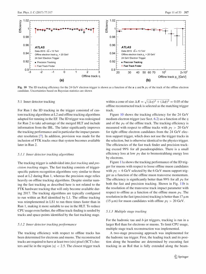
5.1 Inner detector tracking
For Run 1 the ID tracking in the trigger consisted of cus-tom tracking algorithms at L2 and offline tracking algorithmsadapted for running in the EF. The ID trigger was redesignedfor Run 2 to take advantage of the merged HLT and includeinformation from the IBL. The latter significantly improvesthe tracking performance and in particular the impact param-eter resolution [7]. In addition, provision was made for theinclusion of FTK tracks once that system becomes availablelater in Run 2.
5.1.1 Inner detector tracking algorithms
The tracking trigger is subdivided into fast tracking and pre-cision tracking stages. The fast tracking consists of trigger-specific pattern recognition algorithms very similar to thoseused at L2 during Run 1, whereas the precision stage reliesheavily on offline tracking algorithms. Despite similar nam-ing the fast tracking as described here is not related to theFTK hardware tracking that will only become available dur-ing 2017. The tracking algorithms are typically configuredto run within an RoI identified by L1. The offline trackingwas reimplemented in LS1 to run three times faster than inRun 1, making it more suitable to use in the HLT. To reduceCPU usage even further, the offline track-finding is seeded bytracks and space-points identified by the fast tracking stage.
5.1.2 Inner detector tracking performance
The tracking efficiency with respect to offline tracks hasbeen determined for electrons and muons. The reconstructedtracks are required to have at least two (six) pixel (SCT) clus-ters and lie in the region |η| < 2.5. The closest trigger track
within a cone of size �R = √(�η)2 + (�φ)2 = 0.05 of the
offline reconstructed track is selected as the matching triggertrack.
Figure 10 shows the tracking efficiency for the 24 GeVmedium electron trigger (see Sect. 6.2) as a function of the η
and of the pT of the offline track. The tracking efficiency ismeasured with respect to offline tracks with pT > 20 GeVfor tight offline electron candidates from the 24 GeV elec-tron support trigger, which does not use the trigger tracks inthe selection, but is otherwise identical to the physics trigger.The efficiencies of the fast track finder and precision track-ing exceed 99% for all pseudorapidities. There is a smallefficiency loss at low pT due to bremsstrahlung energy lossby electrons.
Figure 11a shows the tracking performance of the ID trig-ger for muons with respect to loose offline muon candidateswith pT > 6 GeV selected by the 6 GeV muon support trig-ger as a function of the offline muon transverse momentum.The efficiency is significantly better than 99% for all pT forboth the fast and precision tracking. Shown in Fig. 11b isthe resolution of the transverse track impact parameter withrespect to offline as a function of the offline muon pT. Theresolution in the fast (precision) tracking is better than 17µm(15 µm) for muon candidates with offline pT > 20 GeV.
5.1.3 Multiple stage tracking
For the hadronic tau and b-jet triggers, tracking is run in alarger RoI than for electrons or muons. To limit CPU usage,multiple stage track reconstruction was implemented.
A two-stage processing approach was implemented forthe hadronic tau trigger. First, the leading track and its posi-tion along the beamline are determined by executing fasttracking in an RoI that is fully extended along the beam-
123

317 Page 12 of 53 Eur. Phys. J. C (2017) 77 :317
[GeV]T
Offline track p5 6 7 8 10 20 30 40 50 210 210×2
Effi
cien
cy
0.96
0.97
0.98
0.99
1
1.01
1.02
Precision Tracking
Fast Track Finder
ATLASData 13 TeV6 GeV Muon Trigger
(a) [GeV]
T
102
Offline p5 6 7 8 20 30 40 50 210×2
reso
lutio
n [m
m]
0d
0.014
0.015
0.016
0.017
0.018
0.019
0.02
0.021
Precision Tracking Fast Track Finder
ATLASData 13 TeV6 GeV Muon Trigger
(b)
10
Fig. 11 The ID tracking performance for the 6 GeV muon trigger; a efficiency as a function of the offline reconstructed muon pT, b the resolutionof the transverse impact parameter, d0 as a function of the offline reconstructed muon pT. Uncertainties based on Bayesian statistics are shown
One-stage tracking RoITwo-stage tracking: 1st stage RoI
Two-stage tracking: 2nd stage RoI
Plan view
beam line
eam line
Fig. 12 A schematic illustrating the RoIs from the single-stage andtwo-stage tau lepton trigger tracking, shown in plan view (x–z plane)along the transverse direction and in perspective view. The z-axis is
along the beam line. The combined tracking volume of the 1st and 2ndstage RoI in the two-stage tracking approach is significantly smallerthan the RoI in the one-stage tracking scheme
line (|z| < 225 mm) but narrow (0.1) in both η and φ.(See the blue-shaded region in Fig. 12.) Using this positionalong the beamline, the second stage reconstructs all tracksin an RoI that is larger (0.4) in both η and φ but limited to|�z| < 10 mm with respect to the leading track. (See thegreen shaded region in Fig. 12.) At this second stage, fasttracking is followed by precision tracking. For evaluationpurposes, the tau lepton signatures can also be executed in asingle-stage mode, running the fast track finder followed bythe precision tracking in an RoI of the full extent along thebeam line and in eta and phi.
Figure 13 shows the performance of the tau two-stagetracking with respect to the offline tau tracking for tracks withpT > 1 GeV originating from decays of offline tau leptoncandidates with pT > 25 GeV, but with very loose trackmatching in�R to the offline tau candidate. Figure 13a showsthe efficiency of the fast tracking from the first and secondstages, together with the efficiency of the precision tracking
for the second stage. The second-stage tracking efficiencyis higher than 96% everywhere, and improves to better than99% for tracks with pT > 2 GeV. The efficiency of the first-stage fast tracking has a slower turn-on, rising from 94% at2 GeV to better than 99% for pT > 5 GeV. This slow turn-onarises due to the narrow width (�φ < 0.1) of the first-stageRoI and the loose tau selection that results in a larger fractionof low-pT tracks from tau candidates that bend out of theRoI (and are not reconstructed) compared to a wider RoI.The transverse impact parameter resolution with respect tooffline for loosely matched tracks is seen in Fig. 13b and isaround 20 µm for tracks with pT > 10 GeV reconstructedby the precision tracking. The tau selection algorithms basedon this two-stage tracking are presented in Sect. 6.5.1.
For b-jet tracking a similar multi-stage tracking strat-egy was adopted. However, in this case the first-stage ver-tex tracking takes all jets identified by the jet trigger withET > 30 GeV and reconstructs tracks with the fast track
123

Eur. Phys. J. C (2017) 77 :317 Page 13 of 53 317
[GeV]T
Offline track p1 2 3 4 5 6 7 10 20 30 210
Effi
cien
cy
0.9
0.92
0.94
0.96
0.98
1
1.02
Fast Track Finder (Stage 1)
Fast Track Finder (Stage 2)
Precision Tracking (Stage 2)
ATLASData 13 TeV
> 1 GeVT
offline track p
25 GeV Tau Trigger
(a)[GeV]
TO ine track p
1 2 3 4 5 6 7 10 20 30 210
reso
lutio
n [m
m]
0d
0.02
0.04
0.06
0.08
0.1
0.12
0.14
0.16
0.18
0.2
Fast Track Finder (Stage 1)
Fast Track Finder (Stage 2)
Precision Tracking (Stage 2)
ATLASData 2015 s = 13 TeV
> 1 GeVT
offline track p
25GeV Tau Trigger
(b)
Fig. 13 The ID trigger tau tracking performance with respect to offlinetracks from very loose tau candidates with pT > 1 GeV from the 25 GeVtau trigger; a the efficiency as a function of the offline reconstructed tautrack pT, b the resolution of the transverse impact parameter, d0 as afunction of the offline reconstructed tau track pT. The offline recon-
structed tau daughter tracks are required to have pT > 1 GeV, lie inthe region |η| < 2.5 and have at least two pixel clusters and at least sixSCT clusters. The closest matching trigger track within a cone of size�R = 0.05 of the offline track is selected as the matching trigger track
Number of tracks
10 20 30 40 50 60 70 80
Ver
tex
ndin
g e
cien
cy
0.2
0.4
0.6
0.8
1
1.2
T
T
> 55 GeV
> 110 GeV> 110 GeV
> 260 GeV> 260 GeVT
Jet trigger E
Jet trigger E
Jet trigger E
ATLASData 2015 s = 13 TeV
offline track pT > 1 GeV
b-jet trigger vertex tracking
(a)Number of tracks
0 10 20 30 40 50 60 70
res
olut
ion
[mm
]0z
0
0.1
0.2
0.3
0.4
0.5
T
T
> 55 GeV
> 110 GeV
> 260 GeVT
Jet E
Jet E
Je E
Data
-jet vertex tracking
(b)
Fig. 14 The trigger performance for primary vertices in the b-jet sig-natures for 55, 110 and 260 GeV jet triggers; a the vertexing efficiencyas a function of the number of offline tracks within the jets used for the
vertex tracking, b the resolution in z of the vertex with respect to theoffline vertex position as a function of the number of offline tracks fromthe offline vertex
finder in a narrow region in η and φ around the jet axis foreach jet, but with |z| < 225 mm along the beam line. Fol-lowing this step, the primary vertex reconstruction [27] isperformed using the tracks from the fast tracking stage. Thisvertex is used to define wider RoIs around the jet axes, with|�η| < 0.4 and |�φ| < 0.4 but with |�z| < 20 mm relativeto the primary vertex z position. These RoIs are then usedfor the second-stage reconstruction that runs the fast trackfinder in the wider η and φ regions followed by the precisiontracking, secondary vertexing and b-tagging algorithms.
The performance of the primary vertexing in the b-jet ver-tex tracking can be seen in Fig. 14a, which shows the vertex
finding efficiency with respect to offline vertices in jet eventswith at least one jet with transverse energy above 55, 110,or 260 GeV and with no additional b-tagging requirement.The efficiency is shown as a function of the number of offlinetracks with pT > 1 GeV that lie within the boundary of thewider RoI (defined above) from the selected jets. The effi-ciency rises sharply and is above 90% for vertices with threeor more tracks, and rises to more than 99.5% for vertices withfive or more tracks. The resolution in z with respect to theoffline z position as shown in Fig. 14b is better than 100 µmfor vertices with two or more offline tracks and improves to60 µm for vertices with ten or more offline tracks.
123
317 Page 14 of 53 Eur. Phys. J. C (2017) 77 :317
Processing time per RoI [ms]0 10 20 30 40 50 60 70 80 90 100
Nor
mal
ised
ent
ries
-610
-510
-410
-310
-210
-110
1ATLASData 2015 s = 13 TeV
Tight 24 GeV electron trigger
Fast Track Finder
Precision Tracking
0.04 ms±mean = 6.2
0.02 ms±mean = 2.5
_
Fig. 15 The CPU processing time for the fast and precision trackingper electron RoI for the 24 GeV electron trigger. The precision trackingis seeded by the tracks found in the fast tracking stage and hence requiresless CPU time
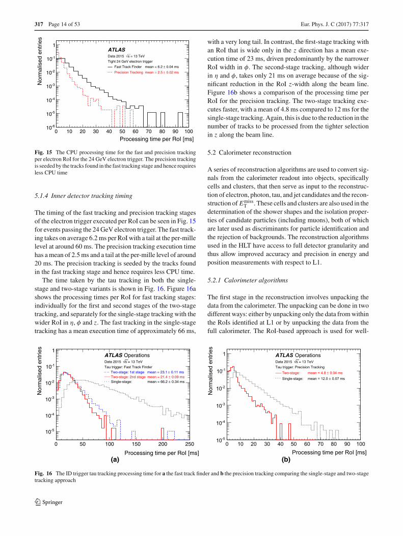
5.1.4 Inner detector tracking timing
The timing of the fast tracking and precision tracking stagesof the electron trigger executed per RoI can be seen in Fig. 15for events passing the 24 GeV electron trigger. The fast track-ing takes on average 6.2 ms per RoI with a tail at the per-millelevel at around 60 ms. The precision tracking execution timehas a mean of 2.5 ms and a tail at the per-mille level of around20 ms. The precision tracking is seeded by the tracks foundin the fast tracking stage and hence requires less CPU time.
The time taken by the tau tracking in both the single-stage and two-stage variants is shown in Fig. 16. Figure 16ashows the processing times per RoI for fast tracking stages:individually for the first and second stages of the two-stagetracking, and separately for the single-stage tracking with thewider RoI in η, φ and z. The fast tracking in the single-stagetracking has a mean execution time of approximately 66 ms,
with a very long tail. In contrast, the first-stage tracking withan RoI that is wide only in the z direction has a mean exe-cution time of 23 ms, driven predominantly by the narrowerRoI width in φ. The second-stage tracking, although widerin η and φ, takes only 21 ms on average because of the sig-nificant reduction in the RoI z-width along the beam line.Figure 16b shows a comparison of the processing time perRoI for the precision tracking. The two-stage tracking exe-cutes faster, with a mean of 4.8 ms compared to 12 ms for thesingle-stage tracking. Again, this is due to the reduction in thenumber of tracks to be processed from the tighter selectionin z along the beam line.
5.2 Calorimeter reconstruction
A series of reconstruction algorithms are used to convert sig-nals from the calorimeter readout into objects, specificallycells and clusters, that then serve as input to the reconstruc-tion of electron, photon, tau, and jet candidates and the recon-struction of Emiss
T . These cells and clusters are also used in thedetermination of the shower shapes and the isolation proper-ties of candidate particles (including muons), both of whichare later used as discriminants for particle identification andthe rejection of backgrounds. The reconstruction algorithmsused in the HLT have access to full detector granularity andthus allow improved accuracy and precision in energy andposition measurements with respect to L1.
5.2.1 Calorimeter algorithms
The first stage in the reconstruction involves unpacking thedata from the calorimeter. The unpacking can be done in twodifferent ways: either by unpacking only the data from withinthe RoIs identified at L1 or by unpacking the data from thefull calorimeter. The RoI-based approach is used for well-
Processing time per RoI [ms]
0 50 100 150 200 250
Nor
mal
ised
nt
ries
-510
-410
-310
-210
-110
1ATLAS OperationsData 13 TeV
Tau trigger: Fast Track Finder_ _ Two-stage: 1st stage mean = 23.1 ± 0.11 ms
Single-stage: mean = 66.2 ± 0.34 ms
___ Two-stage: 2nd stage mean = 21.4 ± 0.09 ms. . .
(a)Processing time per RoI [ms]
0 10 20 30 40 50 60 70 80 90 100
Nor
mal
ised
ntrie
s
-510
-410
-310
-210
-110
1
Two-stage:___ 0.04 ms±mean = 4.8 Single-stage:. . . 0.07 ms±mean = 12.0
ATLAS OperationsData 13 TeVTau trigger: Precision Tracking
(b)
Fig. 16 The ID trigger tau tracking processing time for a the fast track finder and b the precision tracking comparing the single-stage and two-stagetracking approach
123

Eur. Phys. J. C (2017) 77 :317 Page 15 of 53 317
separated objects (e.g. electron, photon, muon, tau), whereasthe full calorimeter reconstruction is used for jets and globalevent quantities (e.g. Emiss
T ). In both cases the raw unpackeddata is then converted into a collection of cells. Two differentclustering algorithms are used to reconstruct the clusters ofenergy deposited in the calorimeter, the sliding-window andthe topo-clustering algorithms [28]. While the latter providesperformance closer to the offline reconstruction, it is alsosignificantly slower (see Sect. 5.2.3).
The sliding-window algorithm operates on a grid in whichthe cells are divided into projective towers. The algorithmscans this grid and positions the window in such a way that thetransverse energy contained within the window is the localmaximum. If this local maximum is above a given threshold,a cluster is formed by summing the cells within a rectan-gular clustering window. For each layer the barycentre ofthe cells within that layer is determined, and then all cellswithin a fixed window around that position are included inthe cluster. Although the size of the clustering window isfixed, the central position of the window may vary slightly ateach calorimeter layer, depending on how the cell energiesare distributed within them.
The topo-clustering algorithm begins with a seed cell anditeratively adds neighbouring cells to the cluster if their ener-gies are above a given energy threshold that is a function ofthe expected root-mean-square (RMS) noise (σ ). The seedcells are first identified as those cells that have energiesgreater than 4σ . All neighbouring cells with energies greaterthan 2σ are then added to the cluster and, finally, all theremaining neighbours to these cells are also added. Unlikethe sliding-window clusters, the topo-clusters have no prede-fined shape, and consequently their size can vary from clusterto cluster.
The reconstruction of candidate electrons and photonsuses the sliding-window algorithm with rectangular cluster-ing windows of size �η × �φ = 0.075×0.175 in the barreland 0.125×0.125 in the end-caps. Since the magnetic fieldbends the electron trajectory in the φ direction, the size of thewindow is larger in that coordinate in order to contain most ofthe energy. The reconstruction of candidate taus and jets andthe reconstruction of Emiss
T all use the topo-clustering algo-rithm. For taus the topo-clustering uses a window of 0.8×0.8around each of the tau RoIs identified at L1. For jets andEmiss
T , the topo-clustering is done for the full calorimeter.In addition, the Emiss
T is also determined based on the cellenergies across the full calorimeter (see Sect. 6.6).
5.2.2 Calorimeter algorithm performance
The harmonisation between the online and offline algorithmsin Run 2 means that the online calorimeter performance isnow much closer to the offline performance. The ET reso-lutions of the sliding-window clusters and the topo-clusterswith respect to their offline counterparts are shown in Fig. 17.The ET resolution of the sliding-window clusters is 3% forclusters above 5 GeV, while the ET resolution of the topo-clustering algorithm is 2% for clusters above 10 GeV. Theslight shift in cell energies between the HLT and offline isdue to the fact that out-of-time pile-up effects were not cor-rected in the online reconstruction, resulting in slightly higherreconstructed cell energies in the HLT (this was changedfor 2016). In addition, the topo-cluster based reconstructionshown in Fig. 17b suffered from a mismatch of some cali-bration constants between online and offline during most of2015, resulting in a shift towards lower HLT cell energies.
(OFF)) * 100T
(HLT) / ET
(OFF) - ET
(E
10− 8− 6− 4− 2− 0 2 4 6 8 10
Ent
ries
0
2
4
6
8
10
10×
ATLAS
= 13 TeVsData 2015,
> 5 GeVTE
RMS = 2.8 %
(a)
(OFF)) * 100T
(HLT) / ET
(OFF) - ET
(E
10− 8− 6− 4− 2− 0 2 4 6 8 10
Ent
ries
0
2
4
6
8
10
12
3310×
ATLAS
= 13 TeVsData 2015,
> 10 GeVTE
RMS = 1.9 %
(b)
Fig. 17 The relative differences between the online and offline ET forasliding-window clusters and b topo-clusters. Online and offline clustersare matched within �R < 0.001. The distribution for the topo-clusters
was obtained from the RoI-based topo-clustering algorithm that is usedfor online tau reconstruction
123

317 Page 16 of 53 Eur. Phys. J. C (2017) 77 :317
Processing time per call [ms]2 4 6 8 10 12 14 16 18 20
Ent
ries
0
5
10
15
20
25
30
35
40
45
50310×
ATLAS
= 13 TeVsData 2015,
<t> = 5.7 ms
(a)Processing time per call [ms]
0 20 40 60 80 100 120 140 160 180 200 220
Ent
ries
0
1
2
3
4
5
6
7
8
9310×
ATLAS
= 13 TeVsData 2015,
<t> = 82 ms
(b)
Fig. 18 The distributions of processing times for the topo-clustering algorithm executed a within an RoI and b on the full calorimeter. Theprocessing times within an RoI are obtained from tau RoIs with a size of �η × �φ = 0.8 × 0.8
5.2.3 Calorimeter algorithm timing
Due to the optimisation of the offline clustering algorithmsduring LS1, offline clustering algorithms can be used in theHLT directly after the L1 selection. At the data preparationstage, a specially optimised infrastructure with a memorycaching mechanism allows very fast unpacking of data, evenfrom the full calorimeter, which comprises approximately187,000 cells. The mean processing time for the data prepa-ration stage is 2 ms per RoI and 20 ms for the full calorime-ter, and both are roughly independent of pile-up. The topo-clustering, however, requires a fixed estimate of the expectedpile-up noise (cell energy contributions from pile-up inter-actions) in order to determine the cluster-building thresholdsand, when there is a discrepancy between the expected pile-up noise and the actual pile-up noise, the processing time canshow some dependence on the pile-up conditions. The meanprocessing time for the topo-clustering is 6 ms per RoI and82 ms for the full calorimeter. The distributions of the topo-clustering processing times are shown in Fig. 18a for an RoIand Fig. 18b for the full calorimeter. The RoI-based topo-clustering can run multiple times if there is more than oneRoI per event. The topo-clustering over the full calorimeterruns at most once per event, even if the event satisfied bothjet and Emiss
T selections at L1. The mean processing time ofthe sliding window clustering algorithm is not shown but istypically less than 2.5 ms per RoI.
5.3 Tracking in the muon spectrometer
Muons are identified at the L1 trigger by the spatial and tem-poral coincidence of hits either in the RPC or TGC cham-bers within the rapidity range of |η| < 2.4. The degree of
deviation from the hit pattern expected for a muon with infi-nite momentum is used to estimate the pT of the muon withsix possible thresholds. The HLT receives this informationtogether with the RoI position and makes use of the preci-sion MDT and CSC chambers to further refine the L1 muoncandidates.
5.3.1 Muon tracking algorithms
The HLT muon reconstruction is split into fast (trigger spe-cific) and precision (close to offline) reconstruction stages,which were used during Run 1 at L2 and EF, respectively.
In the fast reconstruction stage, each L1 muon candidate isrefined by including the precision data from the MDT cham-bers in the RoI defined by the L1 candidate. A track fit isperformed using the MDT drift times and positions, and apT measurement is assigned using lookup tables, creatingMS-only muon candidates. The MS-only muon track is back-extrapolated to the interaction point using the offline trackextrapolator (based on a detailed detector description insteadof the lookup-table-based approach used in Run 1) and com-bined with tracks reconstructed in the ID to form a combinedmuon candidate with refined track parameter resolution.
In the precision reconstruction stage, the muon reconstruc-tion starts from the refined RoIs identified by the fast stage,reconstructing segments and tracks using information fromthe trigger and precision chambers. As in the fast stage, muoncandidates are first formed by using the muon detectors (MS-only) and are subsequently combined with ID tracks leadingto combined muons. If no matching ID track can be found,combined muon candidates are searched for by extrapolatingID tracks to the MS. This latter inside-out approach is slower
123
Eur. Phys. J. C (2017) 77 :317 Page 17 of 53 317
[GeV]T
Offline muon p
20 40 60 80 100 120 140
)of
fline
T)/
(1/p
offli
ne
T -
1/p
onlin
e
T(1
/pσ
3−10
2−10
1−10
Precision Combined BARRELPrecision Combined ENDCAPSPrecision MS-only BARRELPrecision MS-only ENDCAPS
ATLAS = 13 TeVs
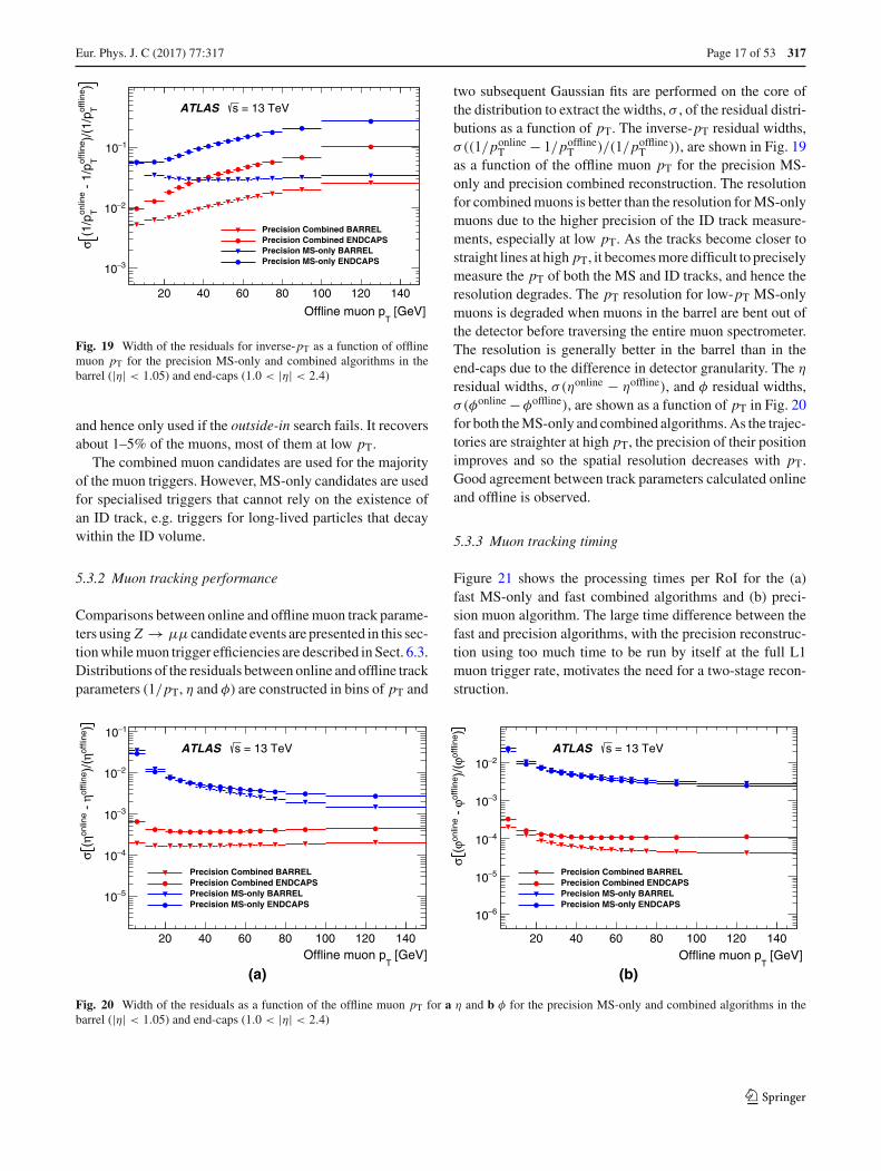
Fig. 19 Width of the residuals for inverse-pT as a function of offlinemuon pT for the precision MS-only and combined algorithms in thebarrel (|η| < 1.05) and end-caps (1.0 < |η| < 2.4)
and hence only used if the outside-in search fails. It recoversabout 1–5% of the muons, most of them at low pT.
The combined muon candidates are used for the majorityof the muon triggers. However, MS-only candidates are usedfor specialised triggers that cannot rely on the existence ofan ID track, e.g. triggers for long-lived particles that decaywithin the ID volume.
5.3.2 Muon tracking performance
Comparisons between online and offline muon track parame-ters using Z → μμ candidate events are presented in this sec-tion while muon trigger efficiencies are described in Sect. 6.3.Distributions of the residuals between online and offline trackparameters (1/pT, η and φ) are constructed in bins of pT and
two subsequent Gaussian fits are performed on the core ofthe distribution to extract the widths, σ , of the residual distri-butions as a function of pT. The inverse-pT residual widths,σ((1/ponline
T − 1/pofflineT )/(1/poffline
T )), are shown in Fig. 19as a function of the offline muon pT for the precision MS-only and precision combined reconstruction. The resolutionfor combined muons is better than the resolution for MS-onlymuons due to the higher precision of the ID track measure-ments, especially at low pT. As the tracks become closer tostraight lines at high pT, it becomes more difficult to preciselymeasure the pT of both the MS and ID tracks, and hence theresolution degrades. The pT resolution for low-pT MS-onlymuons is degraded when muons in the barrel are bent out ofthe detector before traversing the entire muon spectrometer.The resolution is generally better in the barrel than in theend-caps due to the difference in detector granularity. The η
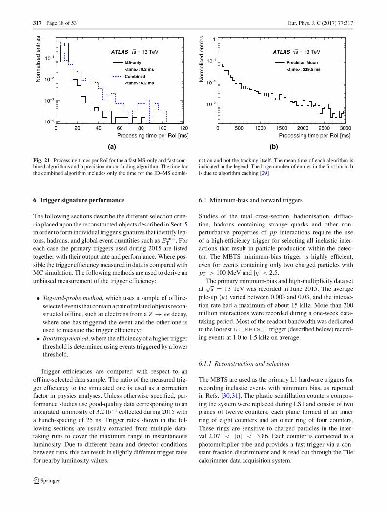
residual widths, σ(ηonline − ηoffline), and φ residual widths,σ(φonline −φoffline), are shown as a function of pT in Fig. 20for both the MS-only and combined algorithms. As the trajec-tories are straighter at high pT, the precision of their positionimproves and so the spatial resolution decreases with pT.Good agreement between track parameters calculated onlineand offline is observed.
5.3.3 Muon tracking timing
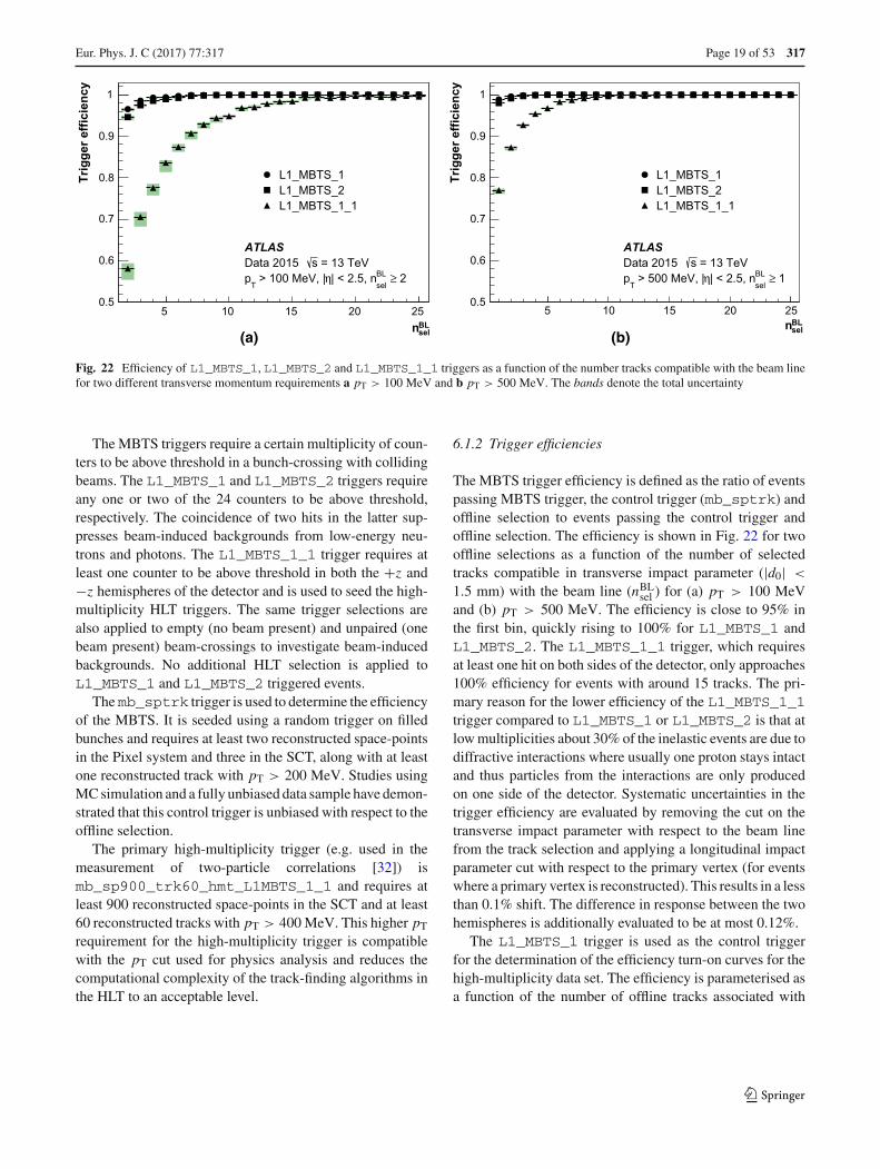
Figure 21 shows the processing times per RoI for the (a)fast MS-only and fast combined algorithms and (b) preci-sion muon algorithm. The large time difference between thefast and precision algorithms, with the precision reconstruc-tion using too much time to be run by itself at the full L1muon trigger rate, motivates the need for a two-stage recon-struction.
[GeV]T
Offline muon p20 40 60 80 100 120 140
)of
fline
η)/
(of
fline
η -
on
line
η(σ
5−10
4−10
3−10
2−10
1−10
Precision Combined BARRELPrecision Combined ENDCAPSPrecision MS-only BARRELPrecision MS-only ENDCAPS
ATLAS = 13 TeVs
(a) [GeV]
TOffline muon p
20 40 60 80 100 120 140
)of
fline
ϕ)/
(of
fline
ϕ -
on
line
ϕ (σ
6−10
5−10
4−10
3−10
2−10
Precision Combined BARRELPrecision Combined ENDCAPSPrecision MS-only BARRELPrecision MS-only ENDCAPS
ATLAS = 13 TeVs
(b)
Fig. 20 Width of the residuals as a function of the offline muon pT for a η and b φ for the precision MS-only and combined algorithms in thebarrel (|η| < 1.05) and end-caps (1.0 < |η| < 2.4)
123
317 Page 18 of 53 Eur. Phys. J. C (2017) 77 :317
Processing time per RoI [ms]0 20 40 60 80 100 120
Nor
mal
ised
ent
ries
4−10
3−10
2−10
1−10MS-only
<time>: 8.2 ms
Combined
<time>: 6.2 ms
ATLAS = 13 TeVs
(a)
Processing time per RoI [ms]0 500 1000 1500 2000 2500 3000
Nor
mal
ised
ent
ries
3−10
2−10
1−10
1
Precision Muon
<time>: 239.5 ms
ATLAS = 13 TeVs
(b)
Fig. 21 Processing times per RoI for the a fast MS-only and fast com-bined algorithms and b precision muon-finding algorithm. The time forthe combined algorithm includes only the time for the ID–MS combi-
nation and not the tracking itself. The mean time of each algorithm isindicated in the legend. The large number of entries in the first bin in bis due to algorithm caching [29]
6 Trigger signature performance
The following sections describe the different selection crite-ria placed upon the reconstructed objects described in Sect. 5in order to form individual trigger signatures that identify lep-tons, hadrons, and global event quantities such as Emiss
T . Foreach case the primary triggers used during 2015 are listedtogether with their output rate and performance. Where pos-sible the trigger efficiency measured in data is compared withMC simulation. The following methods are used to derive anunbiased measurement of the trigger efficiency:
• Tag-and-probe method, which uses a sample of offline-selected events that contain a pair of related objects recon-structed offline, such as electrons from a Z → ee decay,where one has triggered the event and the other one isused to measure the trigger efficiency;
• Bootstrapmethod, where the efficiency of a higher triggerthreshold is determined using events triggered by a lowerthreshold.
Trigger efficiencies are computed with respect to anoffline-selected data sample. The ratio of the measured trig-ger efficiency to the simulated one is used as a correctionfactor in physics analyses. Unless otherwise specified, per-formance studies use good-quality data corresponding to anintegrated luminosity of 3.2 fb−1 collected during 2015 witha bunch-spacing of 25 ns. Trigger rates shown in the fol-lowing sections are usually extracted from multiple data-taking runs to cover the maximum range in instantaneousluminosity. Due to different beam and detector conditionsbetween runs, this can result in slightly different trigger ratesfor nearby luminosity values.
6.1 Minimum-bias and forward triggers
Studies of the total cross-section, hadronisation, diffrac-tion, hadrons containing strange quarks and other non-perturbative properties of pp interactions require the useof a high-efficiency trigger for selecting all inelastic inter-actions that result in particle production within the detec-tor. The MBTS minimum-bias trigger is highly efficient,even for events containing only two charged particles withpT > 100 MeV and |η| < 2.5.
The primary minimum-bias and high-multiplicity data setat
√s = 13 TeV was recorded in June 2015. The average
pile-up 〈μ〉 varied between 0.003 and 0.03, and the interac-tion rate had a maximum of about 15 kHz. More than 200million interactions were recorded during a one-week data-taking period. Most of the readout bandwidth was dedicatedto the loosest L1_MBTS_1 trigger (described below) record-ing events at 1.0 to 1.5 kHz on average.
6.1.1 Reconstruction and selection
The MBTS are used as the primary L1 hardware triggers forrecording inelastic events with minimum bias, as reportedin Refs. [30,31]. The plastic scintillation counters compos-ing the system were replaced during LS1 and consist of twoplanes of twelve counters, each plane formed of an innerring of eight counters and an outer ring of four counters.These rings are sensitive to charged particles in the inter-val 2.07 < |η| < 3.86. Each counter is connected to aphotomultiplier tube and provides a fast trigger via a con-stant fraction discriminator and is read out through the Tilecalorimeter data acquisition system.
123
Eur. Phys. J. C (2017) 77 :317 Page 19 of 53 317
selBLn
5 10 15 20 25
Trig
ger e
ffici
ency
0.5
0.6
0.7
0.8
0.9
1
ATLASData 2015 s = 13 TeV
2≥selBL| < 2.5, nη > 100 MeV, |
Tp
L1_MBTS_1L1_MBTS_2L1_MBTS_1_1
(a)selBLn
5 10 15 20 25
Trig
ger e
ffici
ency
0.5
0.6
0.7
0.8
0.9
1
ATLASData 2015 s = 13 TeV
1≥selBL| < 2.5, nη > 500 MeV, |
Tp
L1_MBTS_1L1_MBTS_2L1_MBTS_1_1
(b)
Fig. 22 Efficiency of L1_MBTS_1, L1_MBTS_2 and L1_MBTS_1_1 triggers as a function of the number tracks compatible with the beam linefor two different transverse momentum requirements a pT > 100 MeV and b pT > 500 MeV. The bands denote the total uncertainty
The MBTS triggers require a certain multiplicity of coun-ters to be above threshold in a bunch-crossing with collidingbeams. The L1_MBTS_1 and L1_MBTS_2 triggers requireany one or two of the 24 counters to be above threshold,respectively. The coincidence of two hits in the latter sup-presses beam-induced backgrounds from low-energy neu-trons and photons. The L1_MBTS_1_1 trigger requires atleast one counter to be above threshold in both the +z and−z hemispheres of the detector and is used to seed the high-multiplicity HLT triggers. The same trigger selections arealso applied to empty (no beam present) and unpaired (onebeam present) beam-crossings to investigate beam-inducedbackgrounds. No additional HLT selection is applied toL1_MBTS_1 and L1_MBTS_2 triggered events.
Themb_sptrk trigger is used to determine the efficiencyof the MBTS. It is seeded using a random trigger on filledbunches and requires at least two reconstructed space-pointsin the Pixel system and three in the SCT, along with at leastone reconstructed track with pT > 200 MeV. Studies usingMC simulation and a fully unbiased data sample have demon-strated that this control trigger is unbiased with respect to theoffline selection.
The primary high-multiplicity trigger (e.g. used in themeasurement of two-particle correlations [32]) ismb_sp900_trk60_hmt_L1MBTS_1_1 and requires atleast 900 reconstructed space-points in the SCT and at least60 reconstructed tracks with pT > 400 MeV. This higher pT
requirement for the high-multiplicity trigger is compatiblewith the pT cut used for physics analysis and reduces thecomputational complexity of the track-finding algorithms inthe HLT to an acceptable level.
6.1.2 Trigger efficiencies
The MBTS trigger efficiency is defined as the ratio of eventspassing MBTS trigger, the control trigger (mb_sptrk) andoffline selection to events passing the control trigger andoffline selection. The efficiency is shown in Fig. 22 for twooffline selections as a function of the number of selectedtracks compatible in transverse impact parameter (|d0| <
1.5 mm) with the beam line (nBLsel ) for (a) pT > 100 MeV
and (b) pT > 500 MeV. The efficiency is close to 95% inthe first bin, quickly rising to 100% for L1_MBTS_1 andL1_MBTS_2. The L1_MBTS_1_1 trigger, which requiresat least one hit on both sides of the detector, only approaches100% efficiency for events with around 15 tracks. The pri-mary reason for the lower efficiency of the L1_MBTS_1_1trigger compared to L1_MBTS_1 or L1_MBTS_2 is that atlow multiplicities about 30% of the inelastic events are due todiffractive interactions where usually one proton stays intactand thus particles from the interactions are only producedon one side of the detector. Systematic uncertainties in thetrigger efficiency are evaluated by removing the cut on thetransverse impact parameter with respect to the beam linefrom the track selection and applying a longitudinal impactparameter cut with respect to the primary vertex (for eventswhere a primary vertex is reconstructed). This results in a lessthan 0.1% shift. The difference in response between the twohemispheres is additionally evaluated to be at most 0.12%.
The L1_MBTS_1 trigger is used as the control triggerfor the determination of the efficiency turn-on curves for thehigh-multiplicity data set. The efficiency is parameterised asa function of the number of offline tracks associated with
123
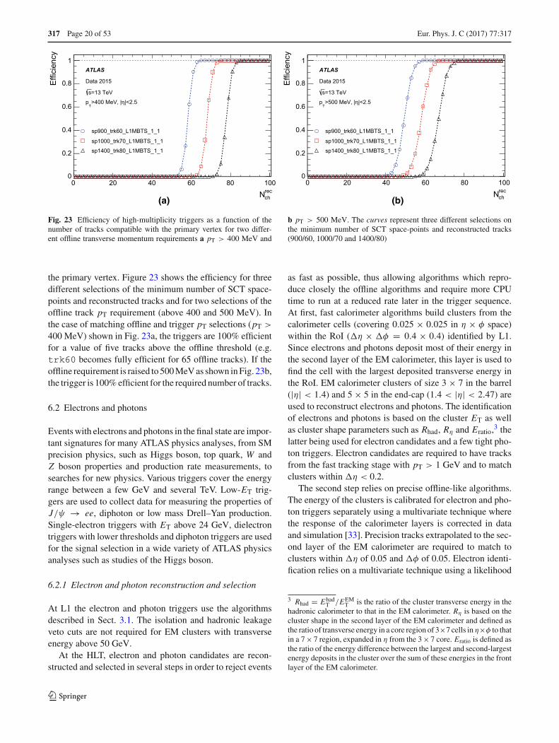
317 Page 20 of 53 Eur. Phys. J. C (2017) 77 :317
recchN
0 20 40 60 80 100
Effi
cien
cy
0
0.2
0.4
0.6
0.8
1ATLAS
Data 2015
=13 TeVs
|<2.5η>400 MeV, |T
p
sp900_trk60_L1MBTS_1_1
sp1000_trk70_L1MBTS_1_1
sp1400_trk80_L1MBTS_1_1
(a)recchN
0 20 40 60 80 100
Effi
cien
cy
0
0.2
0.4
0.6
0.8
1ATLAS
Data 2015
=13 TeVs
|<2.5η>500 MeV, |T
p
sp900_trk60_L1MBTS_1_1
sp1000_trk70_L1MBTS_1_1
sp1400_trk80_L1MBTS_1_1
(b)
Fig. 23 Efficiency of high-multiplicity triggers as a function of thenumber of tracks compatible with the primary vertex for two differ-ent offline transverse momentum requirements a pT > 400 MeV and
b pT > 500 MeV. The curves represent three different selections onthe minimum number of SCT space-points and reconstructed tracks(900/60, 1000/70 and 1400/80)
the primary vertex. Figure 23 shows the efficiency for threedifferent selections of the minimum number of SCT space-points and reconstructed tracks and for two selections of theoffline track pT requirement (above 400 and 500 MeV). Inthe case of matching offline and trigger pT selections (pT >
400 MeV) shown in Fig. 23a, the triggers are 100% efficientfor a value of five tracks above the offline threshold (e.g.trk60 becomes fully efficient for 65 offline tracks). If theoffline requirement is raised to 500 MeV as shown in Fig. 23b,the trigger is 100% efficient for the required number of tracks.
6.2 Electrons and photons
Events with electrons and photons in the final state are impor-tant signatures for many ATLAS physics analyses, from SMprecision physics, such as Higgs boson, top quark, W andZ boson properties and production rate measurements, tosearches for new physics. Various triggers cover the energyrange between a few GeV and several TeV. Low-ET trig-gers are used to collect data for measuring the properties ofJ/ψ → ee, diphoton or low mass Drell–Yan production.Single-electron triggers with ET above 24 GeV, dielectrontriggers with lower thresholds and diphoton triggers are usedfor the signal selection in a wide variety of ATLAS physicsanalyses such as studies of the Higgs boson.
6.2.1 Electron and photon reconstruction and selection
At L1 the electron and photon triggers use the algorithmsdescribed in Sect. 3.1. The isolation and hadronic leakageveto cuts are not required for EM clusters with transverseenergy above 50 GeV.
At the HLT, electron and photon candidates are recon-structed and selected in several steps in order to reject events
as fast as possible, thus allowing algorithms which repro-duce closely the offline algorithms and require more CPUtime to run at a reduced rate later in the trigger sequence.At first, fast calorimeter algorithms build clusters from thecalorimeter cells (covering 0.025 × 0.025 in η × φ space)within the RoI (�η × �φ = 0.4 × 0.4) identified by L1.Since electrons and photons deposit most of their energy inthe second layer of the EM calorimeter, this layer is used tofind the cell with the largest deposited transverse energy inthe RoI. EM calorimeter clusters of size 3 × 7 in the barrel(|η| < 1.4) and 5 × 5 in the end-cap (1.4 < |η| < 2.47) areused to reconstruct electrons and photons. The identificationof electrons and photons is based on the cluster ET as wellas cluster shape parameters such as Rhad, Rη and Eratio,3 thelatter being used for electron candidates and a few tight pho-ton triggers. Electron candidates are required to have tracksfrom the fast tracking stage with pT > 1 GeV and to matchclusters within �η < 0.2.
The second step relies on precise offline-like algorithms.The energy of the clusters is calibrated for electron and pho-ton triggers separately using a multivariate technique wherethe response of the calorimeter layers is corrected in dataand simulation [33]. Precision tracks extrapolated to the sec-ond layer of the EM calorimeter are required to match toclusters within �η of 0.05 and �φ of 0.05. Electron identi-fication relies on a multivariate technique using a likelihood
3 Rhad = EhadT /EEM
T is the ratio of the cluster transverse energy in thehadronic calorimeter to that in the EM calorimeter. Rη is based on thecluster shape in the second layer of the EM calorimeter and defined asthe ratio of transverse energy in a core region of 3×7 cells in η×φ to thatin a 7 × 7 region, expanded in η from the 3 × 7 core. Eratio is defined asthe ratio of the energy difference between the largest and second-largestenergy deposits in the cluster over the sum of these energies in the frontlayer of the EM calorimeter.
123

Eur. Phys. J. C (2017) 77 :317 Page 21 of 53 317
(LH) discriminant with three operating points named looseLH, medium LH and tight LH. An additional working pointnamed very loose LH is used for supporting triggers. The LH-based identification makes use of variables similar to the cut-based identification employed during Run 1 [2] but has betterbackground rejection for the same signal efficiency. The dis-criminating variables used offline are also used by the trigger,exploiting the characteristic features of energy deposits in theEM calorimeters (longitudinal and lateral shower shapes),track quality, track-cluster matching, and particle identifica-tion by the TRT. All variables are described in Refs. [34,35].The composition of the likelihood is the same as in the offlinereconstruction with the exception of momentum loss due tobremsstrahlung, �p/p, which is not accounted for in theonline environment. The photon identification relies only onthe cluster shower-shape variables and three working pointsare also defined: loose, medium and tight.
Not applied during 2015 but foreseen for higher luminosi-ties during Run 2 is an additional requirement on isolationfor the lowest-threshold unprescaled single-electron trigger.The isolation parameter is calculated as the sum of the pT
values of all tracks in a cone of size �R = 0.2 around theelectron for tracks with pT > 1 GeV and |�z0 sin θ | < 0.3,where �z0 is the distance along z between the longitudinalimpact parameter of the track and the leading track in theRoI. The ratio of this quantity to the EM cluster ET, namely∑
pT/ET, is used to estimate the energy deposited by otherparticles.
6.2.2 Electron and photon trigger menu and rates
The primary L1 and HLT electron and photon triggers usedin 2015 are listed in Table 1. The lowest-threshold single-electron trigger (e24_lhmedium_L1EM20VH) applies a24 GeV transverse energy threshold and requires the electronto pass medium LH identification requirements. The triggeris seeded by L1_EM20VH, which requires ET > 20 GeV,and applies an ET-dependent veto against energy depositedin the hadronic calorimeter behind the electromagnetic clus-ter of the electron candidate (hadronic veto, denoted byH in the trigger name). The ET threshold varies slightlyas a function of η to compensate for passive material infront of the calorimeter (denoted by V in the trigger name).To recover efficiency in the high transverse energy regime,this trigger is complemented by a trigger requiring a trans-verse energy above 120 GeV with loose LH identification(e120_lhloose). With a maximum instantaneous lumi-nosity of 5.2×1033 cm−2 s−1 reached during the 2015 data-taking, the rates of electron triggers could be sustained with-out the use of additional electromagnetic or track isolationrequirements at L1 or HLT. The lowest-threshold dielectrontrigger (2e12_lhloose_L12EM10VH) applies a 12 GeVtransverse energy threshold and requires the two electrons
3310×] -1s-2Instantaneous luminosity [cm
0 1 2 3 4 5
Rat
e [k
Hz]
5
10
15
20
25
L1_EM20VHL1_2EM10VHL1_EM22VHIL1_2EM15VH
ATLAS-1L dt = 3.2 fb∫= 13 TeV, s
Fig. 24 L1 trigger rates as a function of the instantaneous luminosityfor selected single- and multi-object triggers
to pass loose LH identification requirements. The trigger isseeded by L1_2EM10VH, which requires two electrons withET above 10 GeV and a hadronic energy veto.
The primary single-photon trigger used in 2015 isg120_loose. It requires a transverse energy above 120 GeVand applies loose photon identification criteria. It is seededby L1_EM22VHI, which requires an isolated electromag-netic cluster (denoted by I in the trigger name) with ET
above 22 GeV and applies a hadronic veto and η-dependentET thresholds as described above. As mentioned earlier, theelectromagnetic isolation and hadronic veto requirements arenot applied for ET above 50 GeV. The two main diphotontriggers areg35_loose_g25_loose, which requires twophotons above 35 and 25 GeV thresholds and loose pho-ton identification requirements, and 2g20_tight, whichrequires two photons with ET above 20 GeV and tight iden-tification. Both triggers are seeded by L1_2EM15VH, whichrequires two electromagnetic clusters with ET above 15 GeVand a hadronic veto.
Figures 24 and 25 show the rates of the electron and photontriggers as a function of the instantaneous luminosity. Thesetrigger rates scale linearly with the instantaneous luminosity.
6.2.3 Electron and photon trigger efficiencies
The performance of electron triggers is studied using a sam-ple of Z → ee events. The tag-and-probe method utilisesevents triggered by a single-electron trigger and requirestwo offline reconstructed electrons with an invariant massbetween 80 and 100 GeV. After identifying the electron thattriggered the event (tag electron), the other electron (probeelectron) is unbiased by the trigger selection, thus allowing itsuse to measure the electron trigger efficiency. HLT electrons(L1 EM objects) are matched to the probe electron if their sep-aration is �R < 0.07(0.15). The trigger efficiency is calcu-
123
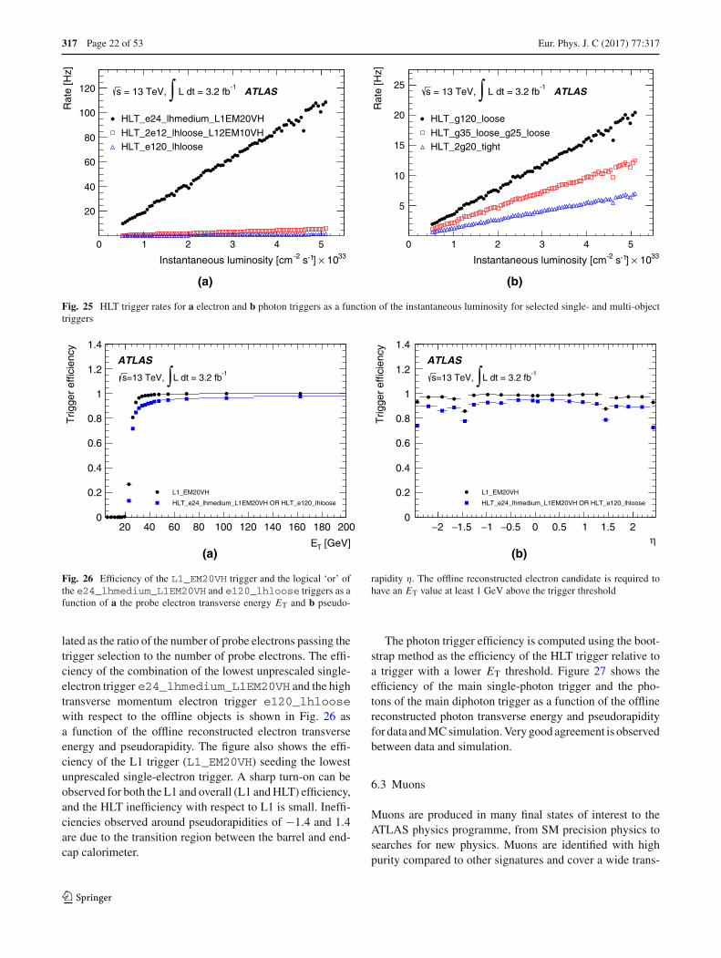
317 Page 22 of 53 Eur. Phys. J. C (2017) 77 :317
3310×] -1s-2Instantaneous luminosity [cm
0 1 2 3 4 5
Rat
e [H
z]
20
40
60
80
100
120
HLT_e24_lhmedium_L1EM20VH
HLT_2e12_lhloose_L12EM10VHHLT_e120_lhloose
ATLAS-1L dt = 3.2 fb∫= 13 TeV, s
(a)
3310×] -1s-2Instantaneous luminosity [cm
0 1 2 3 4 5
Rat
e [H
z]
5
10
15
20
25
HLT_g120_loose
HLT_g35_loose_g25_looseHLT_2g20_tight
ATLAS-1L dt = 3.2 fb∫= 13 TeV, s
(b)
Fig. 25 HLT trigger rates for a electron and b photon triggers as a function of the instantaneous luminosity for selected single- and multi-objecttriggers
[GeV]TE
20 40 60 80 100 120 140 160 180 200
Trig
ger
effic
ienc
y
0
0.2
0.4
0.6
0.8
1
1.2
1.4
L1_EM20VH
HLT_e24_lhmedium_L1EM20VH OR HLT_e120_lhloose
ATLAS-1
L dt = 3.2 fb∫=13 TeV, s
(a)η
2− 1.5− 1− 0.5− 0 0.5 1 1.5 2
Trig
ger
effic
ienc
y
0
0.2
0.4
0.6
0.8
1
1.2
1.4
L1_EM20VH
HLT_e24_lhmedium_L1EM20VH OR HLT_e120_lhloose
ATLAS-1
L dt = 3.2 fb∫=13 TeV, s
(b)
Fig. 26 Efficiency of the L1_EM20VH trigger and the logical ‘or’ ofthe e24_lhmedium_L1EM20VH and e120_lhloose triggers as afunction of a the probe electron transverse energy ET and b pseudo-
rapidity η. The offline reconstructed electron candidate is required tohave an ET value at least 1 GeV above the trigger threshold
lated as the ratio of the number of probe electrons passing thetrigger selection to the number of probe electrons. The effi-ciency of the combination of the lowest unprescaled single-electron trigger e24_lhmedium_L1EM20VH and the hightransverse momentum electron trigger e120_lhloosewith respect to the offline objects is shown in Fig. 26 asa function of the offline reconstructed electron transverseenergy and pseudorapidity. The figure also shows the effi-ciency of the L1 trigger (L1_EM20VH) seeding the lowestunprescaled single-electron trigger. A sharp turn-on can beobserved for both the L1 and overall (L1 and HLT) efficiency,and the HLT inefficiency with respect to L1 is small. Ineffi-ciencies observed around pseudorapidities of −1.4 and 1.4are due to the transition region between the barrel and end-cap calorimeter.
The photon trigger efficiency is computed using the boot-strap method as the efficiency of the HLT trigger relative toa trigger with a lower ET threshold. Figure 27 shows theefficiency of the main single-photon trigger and the pho-tons of the main diphoton trigger as a function of the offlinereconstructed photon transverse energy and pseudorapidityfor data and MC simulation. Very good agreement is observedbetween data and simulation.
6.3 Muons
Muons are produced in many final states of interest to theATLAS physics programme, from SM precision physics tosearches for new physics. Muons are identified with highpurity compared to other signatures and cover a wide trans-
123

Eur. Phys. J. C (2017) 77 :317 Page 23 of 53 317
[GeV]TE20 40 60 80 100 120 140
Trig
ger
effic
ienc
y
0
0.2
0.4
0.6
0.8
1
1.2
1.4 HLT_g20_tight Data MCHLT_g25_loose Data MCHLT_g35_loose Data MCHLT_g120_loose Data MC
ATLAS
= 13 TeV s
(a) η2− 1− 0 1 2
Trig
ger
effic
ienc
y
0
0.2
0.4
0.6
0.8
1
1.2
1.4 HLT_g20_tight Data MCHLT_g25_loose Data MCHLT_g35_loose Data MCHLT_g120_loose Data MC
ATLAS
= 13 TeV s
(b)
Fig. 27 Efficiency of HLT photon triggers g20_tight,g25_loose, g35_loose, and g120_loose relative to a looserHLT photon trigger as a function of a the transverse energy ET andb pseudorapidity η of the photon candidates reconstructed offline and
satisfying the tight identification and isolation requirements. The offlinereconstructed photon candidate is required to have an ET value at least5 GeV above the trigger threshold. The transition region between thebarrel and end-cap calorimeter (1.37 < |η| < 1.52) is excluded
verse momentum range, from a few GeV to several TeV.Muon trigger thresholds in the pT range from 4 to 10 GeVare used to collect data for measurements of processes suchas J/ψ → μμ, low-pT dimuons, and Z → ττ [36,37].Higher pT thresholds are used to collect data for new-physicssearches as well as measuring the properties and productionrates of SM particles such as the Higgs, W and Z bosons,and top quarks [38–40].
6.3.1 Muon reconstruction and selection
The trigger reconstruction algorithms for muons at L1 andthe HLT are described in Sects. 3.2 and 5.3, respectively. Theselection criteria depend on the algorithm used for recon-struction. The MS-only algorithm selects solely on the pT
of the muon candidate measured by the muon spectrometer;the combined algorithm makes selections based on the matchbetween the ID and MS tracks and their combined pT; andthe isolated muon algorithm applies selection criteria basedon the amount of energy in the isolation cones.
6.3.2 Muon trigger menu and rates
The lowest-threshold single-muon trigger (mu20_iloose_L1MU15) requires a minimum transverse momentum of20 GeV for combined muon candidates in addition to a looseisolation: the scalar sum of the track pT values in a cone ofsize �R = 0.2 around the muon candidate is required to besmaller than 12% of the muon transverse momentum. Theisolation requirement reduces the rate by a factor of approx-imately 2.5 with a negligible efficiency loss. The trigger isseeded by L1_MU15, which requires a transverse momen-
tum above 15 GeV. At a transverse momentum above 50 GeVthis trigger is complemented by a trigger not requiring iso-lation (mu50), to recover a small efficiency loss in the hightransverse momentum region.
The lowest-threshold unprescaled dimuon trigger (2mu10)requires a minimum transverse momentum of 10 GeVfor combined muon candidates. The trigger is seeded byL1_2MU10, which requires two muons with transversemomentum above 10 GeV. Figure 28 shows the rates ofthese triggers as a function of the instantaneous luminos-ity. The trigger rates scale linearly with the instantaneousluminosity. Dimuon triggers with lower pT thresholds andfurther selections (e.g. on the dimuon invariant mass) werealso active and are discussed in Sect. 6.8. Additionally, anasymmetric dimuon trigger (mu18_mu8noL1) is included,wheremu18 is seeded byL1_MU15 andmu8noL1performsa search for a muon in the full detector at the HLT. By requir-ing only one muon at L1, the dimuon trigger does not suffera loss of efficiency that would otherwise have if two muonswere required at L1. This trigger is typically used by physicssearches involving two relatively high-pT muons to improvethe acceptance with respect to the standard dimuon triggers.
6.3.3 Muon trigger efficiencies
The L1 and HLT muon efficiencies are determined usinga tag-and-probe method with Z → μμ candidate events.Events are required to contain a pair of reference muons withopposite charge and an invariant mass within 10 GeV of theZ mass. Reference muons reconstructed offline using bothID and MS information are required to be inside the fiducial
123
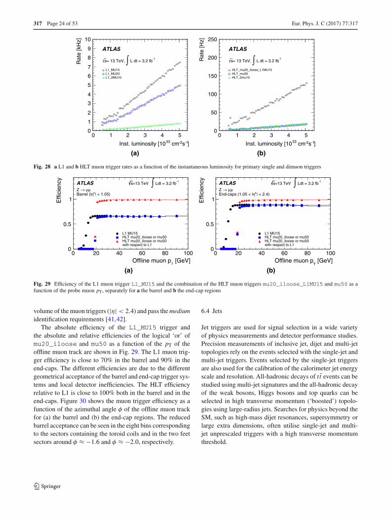
317 Page 24 of 53 Eur. Phys. J. C (2017) 77 :317
]-1s-2cm33Inst. luminosity [10
0 1 2 3 4 5
Rat
e [k
Hz]
0
1
2
3
4
5
6
7
8
9
10
ATLAS
-1L dt = 3.2 fb∫= 13 TeV, s
L1_MU15L1_MU20L1_2MU10
(a)]-1s-2cm33Inst. luminosity [10
0 1 2 3 4 5
Rat
e [H
z]
0
50
100
150
200
250
ATLAS
-1L dt = 3.2 fb∫= 13 TeV, s
HLT_mu20_iloose_L1MU15HLT_mu50HLT_2mu10
(b)
Fig. 28 a L1 and b HLT muon trigger rates as a function of the instantaneous luminosity for primary single and dimuon triggers
[GeV]TO ine muon p0 20 40 60 80 100
Effi
cien
cy
0
0.5
1
L1 MU15HLT mu20_iloose or mu50HLT mu20_iloose or mu50with respect to L1
ATLAS -1Ldt = 3.2 fb∫=13 TeV s
μμ→Z | < 1.05)μηBarrel (|
(a)
[GeV]T
O ine muon p0 20 40 60 80 100
Effi
cien
cy
0
0.5
1
L1 MU15HLT mu20_iloose or mu50HLT mu20_iloose or mu50with respect to L1
ATLAS -1Ldt = 3.2 fb∫=13 TeV s
μμ→Z | < 2.4)μηEnd-caps (1.05 < |
(b)
Fig. 29 Efficiency of the L1 muon trigger L1_MU15 and the combination of the HLT muon triggers mu20_iloose_L1MU15 and mu50 as afunction of the probe muon pT, separately for a the barrel and b the end-cap regions
volume of the muon triggers (|η| < 2.4) and pass themediumidentification requirements [41,42].
The absolute efficiency of the L1_MU15 trigger andthe absolute and relative efficiencies of the logical ‘or’ ofmu20_iloose and mu50 as a function of the pT of theoffline muon track are shown in Fig. 29. The L1 muon trig-ger efficiency is close to 70% in the barrel and 90% in theend-caps. The different efficiencies are due to the differentgeometrical acceptance of the barrel and end-cap trigger sys-tems and local detector inefficiencies. The HLT efficiencyrelative to L1 is close to 100% both in the barrel and in theend-caps. Figure 30 shows the muon trigger efficiency as afunction of the azimuthal angle φ of the offline muon trackfor (a) the barrel and (b) the end-cap regions. The reducedbarrel acceptance can be seen in the eight bins correspondingto the sectors containing the toroid coils and in the two feetsectors around φ ≈ −1.6 and φ ≈ −2.0, respectively.
6.4 Jets
Jet triggers are used for signal selection in a wide varietyof physics measurements and detector performance studies.Precision measurements of inclusive jet, dijet and multi-jettopologies rely on the events selected with the single-jet andmulti-jet triggers. Events selected by the single-jet triggersare also used for the calibration of the calorimeter jet energyscale and resolution. All-hadronic decays of t t events can bestudied using multi-jet signatures and the all-hadronic decayof the weak bosons, Higgs bosons and top quarks can beselected in high transverse momentum (‘boosted’) topolo-gies using large-radius jets. Searches for physics beyond theSM, such as high-mass dijet resonances, supersymmetry orlarge extra dimensions, often utilise single-jet and multi-jet unprescaled triggers with a high transverse momentumthreshold.
123
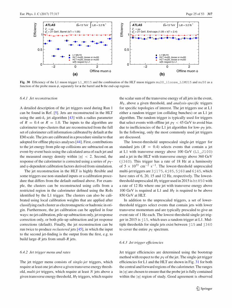
Eur. Phys. J. C (2017) 77 :317 Page 25 of 53 317
φO ine muon 2− 0 2
Effi
cien
cy
0
0.5
1
L1 MU15HLT mu20_iloose or mu50HLT mu20_iloose or mu50with respect to L1
ATLAS -1Ldt = 3.2 fb∫=13 TeV s
μμ→Z | < 1.05)μη> 21 GeV, Barrel (|μ
Tp
(a)φO ine muon
2− 0 2
Effi
cien
cy
0
0.5
1
L1 MU15HLT mu20_iloose or mu50HLT mu20_iloose or mu50with respect to L1
ATLAS -1Ldt = 3.2 fb∫=13 TeV s
μμ→Z | < 2.4)μη> 21 GeV, End-caps (1.05 < |μ
Tp
(b)
Fig. 30 Efficiency of the L1 muon trigger L1_MU15 and the combination of the HLT muon triggers mu20_iloose_L1MU15 and mu50 as afunction of the probe muon φ, separately for a the barrel and b the end-cap regions
6.4.1 Jet reconstruction
A detailed description of the jet triggers used during Run 1can be found in Ref. [5]. Jets are reconstructed in the HLTusing the anti-kt jet algorithm [43] with a radius parameterof R = 0.4 or R = 1.0. The inputs to the algorithm arecalorimeter topo-clusters that are reconstructed from the fullset of calorimeter cell information calibrated by default at theEM scale. The jets are calibrated in a procedure similar to thatadopted for offline physics analyses [44]. First, contributionsto the jet energy from pile-up collisions are subtracted on anevent-by-event basis using the calculated area of each jet andthe measured energy density within |η| < 2. Second, theresponse of the calorimeter is corrected using a series of pT-and η-dependent calibration factors derived from simulation.
The jet reconstruction in the HLT is highly flexible andsome triggers use non-standard inputs or a calibration proce-dure that differs from the default outlined above. For exam-ple, the clusters can be reconstructed using cells from arestricted region in the calorimeter defined using the RoIsidentified by the L1 trigger. The clusters can also be cali-brated using local calibration weights that are applied afterclassifying each cluster as electromagnetic or hadronic in ori-gin. Furthermore, the jet calibration can be applied in fourways: no jet calibration, pile-up subtraction only, jet responsecorrection only, or both pile-up subtraction and jet responsecorrections (default). Finally, the jet reconstruction can berun twice to produce reclustered jets [45], in which the inputto the second jet-finding is the output from the first, e.g. tobuild large-R jets from small-R jets.
6.4.2 Jet trigger menu and rates
The jet trigger menu consists of single-jet triggers, whichrequire at least one jet above a given transverse energy thresh-old, multi-jet triggers, which require at least N jets above agiven transverse energy threshold, HT triggers, which require
the scalar sum of the transverse energy of all jets in the event,HT, above a given threshold, and analysis-specific triggersfor specific topologies of interest. The jet triggers use at L1either a random trigger (on colliding bunches) or an L1 jetalgorithm. The random trigger is typically used for triggersthat select events with offline jet pT < 45 GeV to avoid biasdue to inefficiencies of the L1 jet algorithm for low-pT jets.In the following, only the most commonly used jet triggersare discussed.
The lowest-threshold unprescaled single-jet trigger forstandard jets (R = 0.4) selects events that contain a jetat L1 with transverse energy above 100 GeV (L1_J100)and a jet in the HLT with transverse energy above 360 GeV(j360). This trigger has a rate of 18 Hz at a luminosityof 5 × 1033 cm−2 s−1. The lowest-threshold unprescaledmulti-jet triggers are3j175,4j85,5j60 and 6j45, whichhave rates of 6, 20, 15 and 12 Hz, respectively. The lowest-threshold unprescaled HT trigger used in 2015 isht850witha rate of 12 Hz where one jet with transverse energy above100 GeV is required at L1 and HT is required to be above850 GeV at HLT.
In addition to the unprescaled triggers, a set of lower-threshold triggers select events that contain jets with lowertransverse momentum and are typically prescaled to give anevent rate of 1 Hz each. The lowest-threshold single-jet trig-ger in 2015 is j15, which uses a random trigger at L1. Mul-tiple thresholds for single jets exist between j15 and j360to cover the entire pT spectrum.
6.4.3 Jet trigger efficiencies
Jet trigger efficiencies are determined using the bootstrapmethod with respect to the pT of the jet. The single-jet triggerefficiencies for L1 and the HLT are shown in Fig. 31 for boththe central and forward regions of the calorimeter. The rangesin |η| are chosen to ensure that the probe jet is fully containedwithin the |η| region of study. Good agreement is observed
123

317 Page 26 of 53 Eur. Phys. J. C (2017) 77 :317
[GeV]T
Leading central jet p0 50 100 150 200 250 300
Effi
cien
cy
0
0.2
0.4
0.6
0.8
1
1.2L1_J20L1_J50L1_J75L1_J100
DataDataDataData
ATLASs = 13 TeV| < 2.6η|
(a) [GeV]
TLeading forward jet p
0 50 100 150 200 250
Effi
cien
cy
0
0.2
0.4
0.6
0.8
1
1.2L1_J20.31ETA49L1_J50.31ETA49L1_J75.31ETA49L1_J100.31ETA49
DataDataDataData
ATLASs = 13 TeV
| < 4.5η3.6 < |
(b)
[GeV]T
Leading central jet p0 50 100 150 200 250 300 350 400 450 500
Effi
cien
cy
0
0.2
0.4
0.6
0.8
1
1.2HLT_j25HLT_j60HLT_j175HLT_j360
DataDataDataData
SimulationSimulationSimulationSimulation
ATLASs = 13 TeV| < 2.8η|
(c)
[GeV]T
Leading forward jet p0 50 100 150 200 250
Effi
cien
cy
0
0.2
0.4
0.6
0.8
1
1.2HLT_j25_320eta490HLT_j60_320eta490HLT_j110_320eta490HLT_j175_320eta490
DataDataDataData
SimulationSimulationSimulationSimulation
ATLASs = 13 TeV
| < 4.5η3.6 < |
(d)
Fig. 31 Efficiency of single-jet triggers as a function of offline jet pT for a L1 in the central region, b L1 in the forward region, c HLT in the centralregion, and d HLT in the forward region
between simulation and data. The sharp HLT efficiency turn-on curves in Fig. 31 are due to good agreement betweenthe energy scale of jets in the HLT and offline, as shown inFig. 32.
The multi-jet trigger efficiencies are dominated by the trig-ger efficiency of the N th leading jet and are shown in Fig. 33for (a) L1 and (b) HLT as a function of the N th leadingjet transverse momentum. Good agreement is found for theefficiency as a function of the N th jet for different jet multi-plicities with the same threshold (e.g. L1_6J15, L1_4J15and 4j45, 5j45) and between data and simulation for theHLT.
Finally, the efficiency of the HT and large-R (R = 1.0)triggers are shown in Fig. 34. The HT trigger efficienciesare measured with respect to the HLT_j150_L1J40 trig-ger. There is a small offset in the efficiency curves for dataand simulation for both thresholds. For the large-R trig-
[GeV]T
p100 150 200 250 300 350 400 450 500
offli
ne
T /
pH
LTTp
0.7
0.8
0.9
1
1.1
1.2
1.3
10
210
310
ATLASEvents passing HLT_j60 trigger
| < 2.8 > 85 GeV, |T
p
Fig. 32 Comparison between the jet energy scales of trigger and offlinejets. The black points represent the mean of the distribution at a givenpT value. The 2% shift is due to differences in the jet calibration appliedonline and offline
123
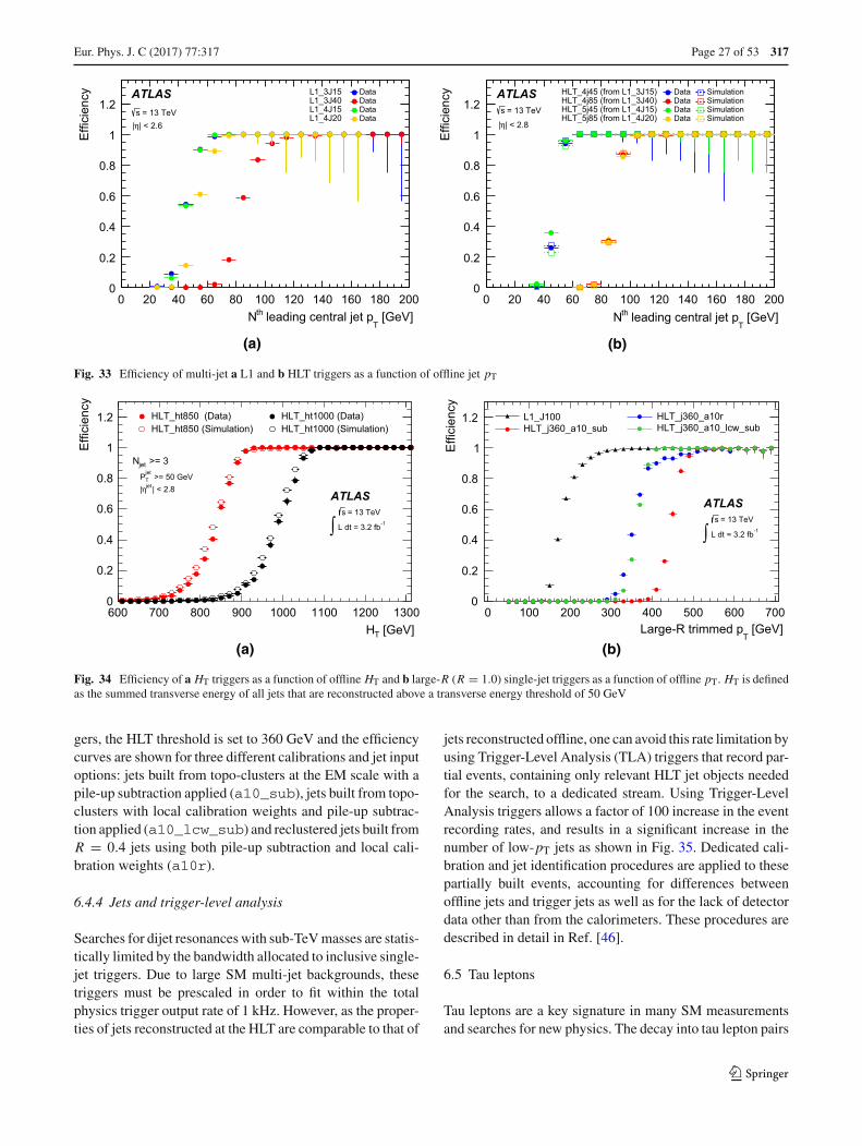
Eur. Phys. J. C (2017) 77 :317 Page 27 of 53 317
[GeV]T
leading central jet pthN0 20 40 60 80 100 120 140 160 180 200
Effi
cien
cy
0
0.2
0.4
0.6
0.8
1
1.2L1_3J15L1_3J40L1_4J15L1_4J20
DataDataDataData
ATLASs = 13 TeV| < 2.6η|
(a)
[GeV]T
leading central jet pthN0 20 40 60 80 100 120 140 160 180 200
Effi
cien
cy
0
0.2
0.4
0.6
0.8
1
1.2HLT_4j45 (from L1_3J15)HLT_4j85 (from L1_3J40)HLT_5j45 (from L1_4J15)HLT_5j85 (from L1_4J20)
DataDataDataData
SimulationSimulationSimulationSimulation
ATLASs = 13 TeV
| < 2.8η|
(b)
Fig. 33 Efficiency of multi-jet a L1 and b HLT triggers as a function of offline jet pT
[GeV]TH600 700 800 900 1000 1100 1200 1300
Effi
cien
cy
0
0.2
0.4
0.6
0.8
1
1.2 HLT_ht850 (Data)HLT_ht850 (Simulation)
HLT_ht1000 (Data)HLT_ht1000 (Simulation)
ATLAS
>= 3 jetN >= 50 GeV
jetTP
| < 2.8jetη|
= 13 TeVs-1 L dt = 3.2 fb∫
(a) [GeV]
TLarge-R trimmed p
0 100 200 300 400 500 600 700
Effi
cien
cy
0
0.2
0.4
0.6
0.8
1
1.2
ATLASs = 13 TeV
-1L dt = 3.2 fb∫
(b)
Fig. 34 Efficiency of a HT triggers as a function of offline HT and b large-R (R = 1.0) single-jet triggers as a function of offline pT. HT is definedas the summed transverse energy of all jets that are reconstructed above a transverse energy threshold of 50 GeV
gers, the HLT threshold is set to 360 GeV and the efficiencycurves are shown for three different calibrations and jet inputoptions: jets built from topo-clusters at the EM scale with apile-up subtraction applied (a10_sub), jets built from topo-clusters with local calibration weights and pile-up subtrac-tion applied (a10_lcw_sub) and reclustered jets built fromR = 0.4 jets using both pile-up subtraction and local cali-bration weights (a10r).
6.4.4 Jets and trigger-level analysis
Searches for dijet resonances with sub-TeV masses are statis-tically limited by the bandwidth allocated to inclusive single-jet triggers. Due to large SM multi-jet backgrounds, thesetriggers must be prescaled in order to fit within the totalphysics trigger output rate of 1 kHz. However, as the proper-ties of jets reconstructed at the HLT are comparable to that of
jets reconstructed offline, one can avoid this rate limitation byusing Trigger-Level Analysis (TLA) triggers that record par-tial events, containing only relevant HLT jet objects neededfor the search, to a dedicated stream. Using Trigger-LevelAnalysis triggers allows a factor of 100 increase in the eventrecording rates, and results in a significant increase in thenumber of low-pT jets as shown in Fig. 35. Dedicated cali-bration and jet identification procedures are applied to thesepartially built events, accounting for differences betweenoffline jets and trigger jets as well as for the lack of detectordata other than from the calorimeters. These procedures aredescribed in detail in Ref. [46].
6.5 Tau leptons
Tau leptons are a key signature in many SM measurementsand searches for new physics. The decay into tau lepton pairs
123

317 Page 28 of 53 Eur. Phys. J. C (2017) 77 :317
[GeV]T
Leading jet p
22×10
23×10
24×10
310
Num
ber
of je
ts /
[GeV
]
1
10
210
310
410
ATLAS-1= 13 TeV, 6.25 pbs
2015 Data: Single Run
Fig. 35 Jet pT spectrum after the basic kinematic selection for the TLAtrigger jets (black) compared to trigger jets recorded by all single-jettriggers (blue)
provides the strongest signal for measurements of the SMHiggs boson coupling to fermions. Final states containingtau leptons are also often favoured by heavier Higgs bosonsor other new resonances in many scenarios beyond the SM.Most (about 65%) of tau leptons decay hadronically. Hencean efficient trigger on hadronic tau decays is crucial for manyanalyses using tau leptons.
Dedicated tau trigger algorithms were designed and imple-mented based on the main features of hadronic tau decays:narrow calorimeter energy deposits and a small number ofassociated tracks. Due to the high production rate of jets withfeatures very similar to hadronic tau decays, keeping the rateof tau triggers under control is particularly challenging.
6.5.1 Tau reconstruction and selection
At L1 the tau trigger uses the algorithms described inSect. 3.1. The isolation requirement was tuned with 13 TeVsimulation to yield an efficiency of 98% and is not appliedfor tau candidates with a transverse energy above 60 GeV.
At the HLT three sequential selections are made. First, aminimum requirement is applied to the transverse energy ofthe tau candidate. The energy is calculated using the locallycalibrated topo-clusters of calorimeter cells contained in acone of size �R = 0.2 around the L1 tau RoI directiontaken from the L1 cluster. A dedicated tau energy calibrationscheme is used. Second, two-stage fast tracking (Sect. 5.1.3)is used to select tau candidates with low track multiplicity.A leading track is sought within a narrow cone (�R = 0.1)around the tau direction followed by a second fast trackingstep using a larger cone (�R = 0.4) but with the tracksrequired to originate from within a fixed interval along thebeam line around the leading track. Tracks with pT > 1 GeVare counted in the core cone region �R < 0.2 and in the
isolation annulus 0.2 < �R < 0.4 around the tau candi-date direction. A track multiplicity requirement selects taucandidates with 1 ≤ N trk
�R<0.2 ≤ 3 and N trk0.2<�R<0.4 ≤ 1.
Finally, the HLT precision tracking is run, and a collection ofvariables built from calorimeter and track variables are inputto a Boosted Decision Tree (BDT), which produces a scoreused for the final tau identification. The implementation ofthose variables follows closely their offline counterparts asdescribed in Ref. [47]. In addition, the same BDT trainingis used offline and online to ensure a maximal correlationbetween online and offline identification criteria. The per-formance of the offline training was found to be comparableto a dedicated online training. To ensure a robust responseunder differing pile-up conditions, corrections as a functionof the average number of interactions per bunch-crossing areapplied to the discriminating variables. Working points ofthe BDT are tuned separately for 1-prong and 3-prong can-didates. The baseline medium working point operates withan efficiency of 95% (70%) for true 1-prong (3-prong) taus.
6.5.2 Tau trigger menu and rates
The primary tau triggers consist of triggers for single hightransverse momentum taus, and combined τ + X triggers,where X stands for an electron, muon, a second tau or Emiss
T .The transverse momentum thresholds used in the single-tauand ditau triggers in 2015 are indicated in Table 1. For all tautriggers the L1 isolation, HLT track multiplicity and onlinemedium identification requirements are applied to the taucandidates.
Due to L1 rate limitations, the combined triggers τ+(e, μ)
and τ+EmissT require the presence of an additional jet candi-
date at L1 with transverse momentum above 25 and 20 GeV,respectively. Variants of these triggers with higher thresh-olds for the tau transverse momentum and without the L1 jetrequirement are also included in the trigger menu. Figure 36shows the L1 and HLT output rates as function of the instan-taneous luminosity for the primary single-tau, ditau, τ + e,τ + μ and τ+Emiss
T triggers.
6.5.3 Tau trigger efficiencies
The efficiency of the tau trigger was measured using a tag-and-probe (T&P) method in an enriched sample of Z →τμτhad → μ + 2ν + τhad events, where τμ is a tau leptondecaying to μνν and τhad is a tau lepton decaying hadroni-cally. Events are selected by the lowest unprescaled single-muon trigger and are tagged by an offline reconstructed andisolated muon with transverse momentum above 22 GeV.The presence of an offline reconstructed tau candidate withtransverse momentum above 25 GeV, one or three tracks,fulfilling the medium identification criteria and with elec-tric charge opposite to the muon charge is also required. This
123
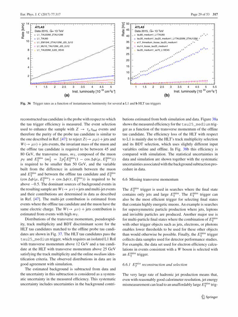
Eur. Phys. J. C (2017) 77 :317 Page 29 of 53 317
]-1s-2 cm33Inst. luminosity [101 1.5 2 2.5 3 3.5 4 4.5 5
Rat
e [k
Hz]
2
4
6
8
10
12
14
= 13 TeVsData 2015, ATLAS
L1_TAU20IM_2TAU12IM
L1_TAU60
L1_EM15HI_2TAU12IM_J25_3J12
L1_MU10_TAU12IM_J25_2J12
L1_TAU20IM_2J20_XE45
(a)]-1s-2 cm33Inst. luminosity [10
1 1.5 2 2.5 3 3.5 4 4.5 5 5.5
Rat
e [H
z]
5
10
15
20
25
30
35
40
45
50
= 13 TeVsData 2015, ATLAS
tau80_medium1_L1TAU60
tau35_medium1_tau25_medium1_L1TAU20IM_2TAU12IM
e17_lhmedium_iloose_tau25_medium1
mu14_iloose_tau25_medium1
tau35_medium1_xe70_L1XE45
(b)
Fig. 36 Trigger rates as a function of instantaneous luminosity for several a L1 and b HLT tau triggers
reconstructed tau candidate is the probe with respect to whichthe tau trigger efficiency is measured. The event selectionused to enhance the sample with Z → τμτhad events andtherefore the purity of the probe tau candidate is similar tothe one described in Ref. [47]: to reject Z(→ μμ)+ jets andW (→ μν) + jets events, the invariant mass of the muon andthe offline tau candidate is required to be between 45 and80 GeV, the transverse mass, mT, composed of the muonpT and Emiss
T (m2T = 2pμ
T EmissT (1 − cos �φ(μ, Emiss
T )))is required to be smaller than 50 GeV, and the variablebuilt from the difference in azimuth between the muonand Emiss
T and between the offline tau candidate and EmissT
(cos �φ(μ, EmissT ) + cos �φ(τ, Emiss
T )) is required to beabove −0.5. The dominant sources of background events inthe resulting sample areW (→ μν)+jets and multi-jet eventsand their contributions are determined in data as describedin Ref. [47]. The multi-jet contribution is estimated fromevents where the offline tau candidate and the muon have thesame electric charge. The W (→ μν) + jets contribution isestimated from events with high mT.
Distributions of the transverse momentum, pseudorapid-ity, track multiplicity and BDT discriminant score for theHLT tau candidates matched to the offline probe tau candi-dates are shown in Fig. 37. The HLT tau candidates pass thetau25_medium trigger, which requires an isolated L1 RoIwith transverse momentum above 12 GeV and a tau candi-date at the HLT with transverse momentum above 25 GeVsatisfying the track multiplicity and the online medium iden-tification criteria. The observed distributions in data are ingood agreement with simulation.
The estimated background is subtracted from data andthe uncertainty in this subtraction is considered as a system-atic uncertainty in the measured efficiency. This systematicuncertainty includes uncertainties in the background contri-
butions estimated from both simulation and data. Figure 38ashows the measured efficiency for thetau25_medium trig-ger as a function of the transverse momentum of the offlinetau candidate. The efficiency loss of the HLT with respectto L1 is mainly due to the HLT’s track multiplicity selectionand its BDT selection, which uses slightly different inputvariables online and offline. In Fig. 38b this efficiency iscompared with simulation. The statistical uncertainties indata and simulation are shown together with the systematicuncertainties associated with the background subtraction pro-cedure in data.
6.6 Missing transverse momentum
The EmissT trigger is used in searches where the final state
contains only jets and large EmissT . The Emiss
T trigger canalso be the most efficient trigger for selecting final statesthat contain highly energetic muons. An example is searchesfor supersymmetric particle production where jets, leptonsand invisible particles are produced. Another major use isfor multi-particle final states where the combination of Emiss
Twith other trigger objects such as jets, electrons, or photonsenables lower thresholds to be used for these other objectsthan would otherwise be possible. Finally, the Emiss
T triggercollects data samples used for detector performance studies.For example, the data set used for electron efficiency calcu-lations in events consistent with a W boson is selected withan Emiss
T trigger.
6.6.1 EmissT reconstruction and selection
The very large rate of hadronic jet production means that,even with reasonably good calorimeter resolution, jet energymismeasurement can lead to an unaffordably large Emiss
T trig-
123
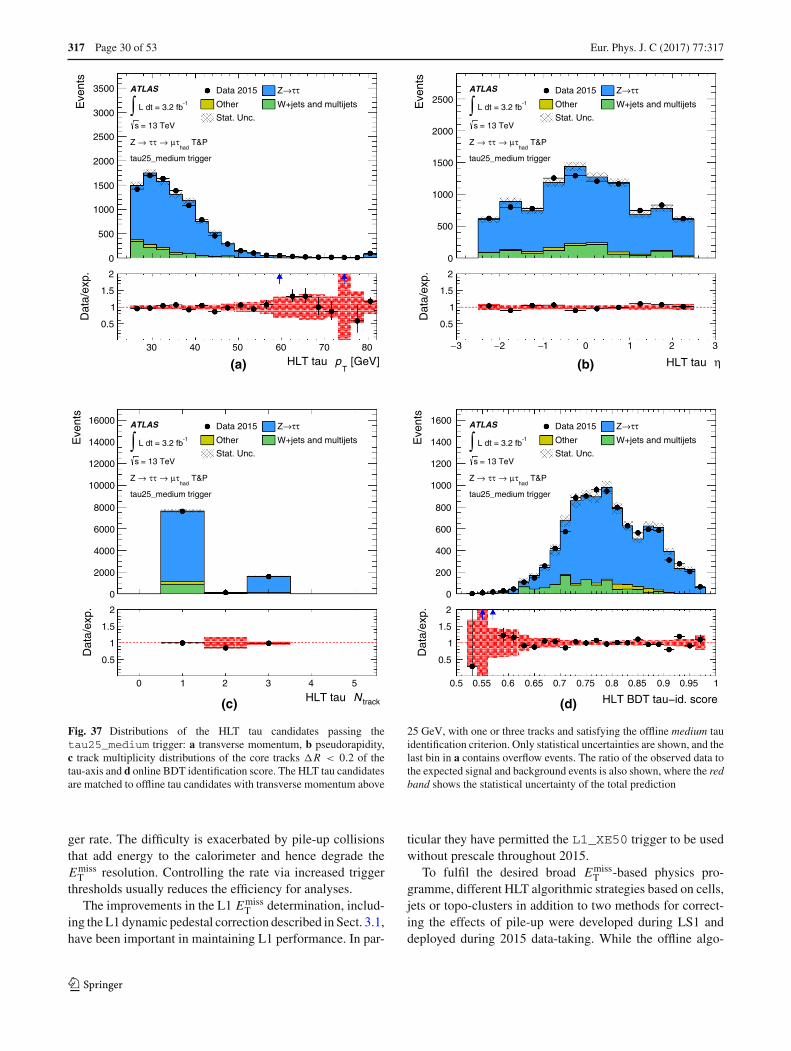
317 Page 30 of 53 Eur. Phys. J. C (2017) 77 :317
Eve
nts
0
500
1000
1500
2000
2500
3000
3500 ATLAS
-1 L dt = 3.2 fb∫ = 13 TeVs
T&Phad
τμ→ττ→Z
tau25_medium trigger
Data 2015 ττ→Z
Other W+jets and multijets
Stat. Unc.
[GeV]T
pHLT tau 30 40 50 60 70 80
Dat
a/ex
p.
0.5
1
1.5
2
(a)
Eve
nts
0
500
1000
1500
2000
2500ATLAS
-1 L dt = 3.2 fb∫ = 13 TeVs
T&Phad
τμ→ττ→Z
tau25_medium trigger
Data 2015 ττ→Z
Other W+jets and multijets
Stat. Unc.
ηHLT tau
3− 2− 1− 0 1 2 3
Dat
a/ex
p.
0.5
1
1.5
2
(b)
Eve
nts
0
2000
4000
6000
8000
10000
12000
14000
16000 ATLAS
-1 L dt = 3.2 fb∫ = 13 TeVs
T&Phad
τμ→ττ→Z
tau25_medium trigger
Data 2015 ττ→Z
Other W+jets and multijets
Stat. Unc.
trackNHLT tau 0 1 2 3 4 5
Dat
a/ex
p.
0.5
1
1.5
2
(c)
Eve
nts
0
200
400
600
800
1000
1200
1400
1600 ATLAS
-1 L dt = 3.2 fb∫ = 13 TeVs
T&Phad
τμ→ττ→Z
tau25_medium trigger
Data 2015 ττ→Z
Other W+jets and multijets
Stat. Unc.
HLT BDT tau−id. score
0.5 0.55 0.6 0.65 0.7 0.75 0.8 0.85 0.9 0.95 1
Dat
a/ex
p.
0.5
1
1.5
2
(d)
Fig. 37 Distributions of the HLT tau candidates passing thetau25_medium trigger: a transverse momentum, b pseudorapidity,c track multiplicity distributions of the core tracks �R < 0.2 of thetau-axis and d online BDT identification score. The HLT tau candidatesare matched to offline tau candidates with transverse momentum above
25 GeV, with one or three tracks and satisfying the offline medium tauidentification criterion. Only statistical uncertainties are shown, and thelast bin in a contains overflow events. The ratio of the observed data tothe expected signal and background events is also shown, where the redband shows the statistical uncertainty of the total prediction
ger rate. The difficulty is exacerbated by pile-up collisionsthat add energy to the calorimeter and hence degrade theEmiss
T resolution. Controlling the rate via increased triggerthresholds usually reduces the efficiency for analyses.
The improvements in the L1 EmissT determination, includ-
ing the L1 dynamic pedestal correction described in Sect. 3.1,have been important in maintaining L1 performance. In par-
ticular they have permitted the L1_XE50 trigger to be usedwithout prescale throughout 2015.
To fulfil the desired broad EmissT -based physics pro-
gramme, different HLT algorithmic strategies based on cells,jets or topo-clusters in addition to two methods for correct-ing the effects of pile-up were developed during LS1 anddeployed during 2015 data-taking. While the offline algo-
123
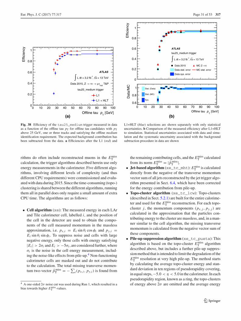
Eur. Phys. J. C (2017) 77 :317 Page 31 of 53 317
[GeV]T
pOffline tau 0 10 20 30 40 50 60 70 80 90 100
Effi
cien
cy
0
0.2
0.4
0.6
0.8
1
ATLAS
= 13 TeVs, -1
L dt = 3.2 fb∫ T&P
hadτμ→ττ→Data 2015, Z
tau25_medium trigger
L1
L1 + HLT
(a)
Effi
cien
cy
0
0.2
0.4
0.6
0.8
1
ATLAS
tau25_medium trigger
= 13 TeVs, -1
L dt = 3.2 fb∫Data 2015 ττ→MC Z
Data stat. error MC stat. error
Data sys. error
[GeV]T
pOffline tau
0 10 20 30 40 50 60 70 80 90 100
Dat
a/M
C
0.6
0.8
1 Stat. (Data)
Stat. (MC)
Sys.
(b)
Fig. 38 Efficiency of the tau25_medium trigger measured in dataas a function of the offline tau pT for offline tau candidates with pTabove 25 GeV, one or three tracks and satisfying the offline mediumidentification requirement. The expected background contribution hasbeen subtracted from the data. a Efficiencies after the L1 (red) and
L1+HLT (blue) selections are shown separately with only statisticaluncertainties. b Comparison of the measured efficiency after L1+HLTto simulation. Statistical uncertainties associated with data and simu-lation and the systematic uncertainty associated with the backgroundsubtraction procedure in data are shown
rithms do often include reconstructed muons in the EmissT
calculation, the trigger algorithms described herein use onlyenergy measurements in the calorimeter. Five different algo-rithms, involving different levels of complexity (and thusdifferent CPU requirements) were commissioned and evalu-ated with data during 2015. Since the time-consuming (topo-)clustering is shared between the different algorithms, runningthem all in parallel does only require a small amount of extraCPU time. The algorithms are as follows:
• Cell algorithm (xe): The measured energy in each LArand Tile calorimeter cell, labelled i , and the position ofthe cell in the detector are used to obtain the compo-nents of the cell measured momentum in the masslessapproximation, i.e. px,i = Ei sin θi cos φi and py,i =Ei sin θi sin φi . To suppress noise and cells with largenegative energy, only those cells with energy satisfying|Ei | > 2σi and Ei > −5σi , are considered further, whereσi is the noise in the cell energy measurement, includ-ing the noise-like effects from pile-up.4 Non-functioningcalorimeter cells are masked out and do not contributeto the calculation. The total missing transverse momen-tum two-vector pmiss
T = −∑i (px,i , py,i ) is found from
4 A one-sided 2σ noise cut was used during Run 1, which resulted in abias towards higher Emiss
T -values.
the remaining contributing cells, and the EmissT calculated
from its norm EmissT = | pmiss
T |.• Jet-based algorithm (xe_tc_mht): Emiss
T is calculateddirectly from the negative of the transverse momentumvector sum of all jets reconstructed by the jet trigger algo-rithm presented in Sect. 6.4, which have been correctedfor the energy contribution from pile-up.
• Topo-cluster algorithm (xe_tc_lcw): Topo-clusters(described in Sect. 5.2.1) are built for the entire calorime-ter and used for the Emiss
T reconstruction. For each topo-cluster j , the momentum components (px, j , py, j ) arecalculated in the approximation that the particles con-tributing energy to the cluster are massless, and, in a man-ner similar to the cell algorithm, the missing transversemomentum is calculated from the negative vector sum ofthese components.
• Pile-up suppression algorithm (xe_tc_pueta): Thisalgorithm is based on the topo-cluster Emiss
T algorithmdescribed above, but includes a further pile-up suppres-sion method that is intended to limit the degradation of theEmiss
T resolution at very high pile-up. The method startsby calculating the average topo-cluster energy and stan-dard deviation in ten regions of pseudorapidity covering,in equal steps, −5.0 < η < 5.0 in the calorimeter. In eachpseudorapidity region, known as a ring, the topo-clustersof energy above 2σ are omitted and the average energy
123

317 Page 32 of 53 Eur. Phys. J. C (2017) 77 :317
of the residual topo-clusters is calculated. This averagerepresents an estimate of the energy contribution frompile-up in that ring. The pile-up energy density in eachring is obtained by dividing the average energy by thesolid angle of the ring. This energy density is then mul-tiplied by the solid angle of each topo-cluster and thensubtracted from the energy of that topo-cluster to obtaina topo-cluster energy measurement corrected for pile-up.The Emiss
T is recalculated as described above using the(px, j , py, j ) of topo-clusters after the pile-up subtraction.
• Pile-up fit algorithm (xe_tc_pufit): Starting againfrom the topo-cluster Emiss
T described above, a differ-ent pile-up suppression method is used in this algorithm.The calorimeter is partitioned into 112 towers each of sizeη×φ ≈ 0.71×0.79. For each tower, the px and py com-ponents of all the topo-clusters with centres in that towerare summed to obtain the transverse momentum pT,k ofthat kth tower. The transverse energy sum of the towerET,k is also calculated from the scalar sum of the pT ofthe individual clusters. If ET,k < 45 GeV, the tower isdetermined to be below threshold and its energy assumedto be due to pile-up. The average pile-up ET density iscalculated from
∑k ET,k/
∑k Ak of all the towers below
threshold, where Ak is the total area in (η, φ) coordinatesof those towers. A fit estimates the ET contributed bypile-up in each tower above threshold using the averagepile-up ET density and constraining the event-wide Emiss
Tfrom pile-up to be zero within resolution. These estimatedpile-up contributions are subtracted from the correspond-ing ET measurements for towers above threshold, andthese corrected ET values are used to calculate Emiss
T .
Figure 39 shows the EmissT distribution of the various HLT
algorithms for events accepted into the Main physics stream.The differences observed between the cell-based and thetopo-cluster-based Emiss
T distributions are caused in part bydifferent calibration; the cell-based algorithm is calibrated atthe EM scale, while algorithms based on topo-clusters gen-erally have larger values of Emiss
T as they include a correc-tion for the calorimeter response to hadrons (hadronic scale).Differences between the Emiss
T distributions for the variouspile-up correction schemes are small, since these algorithmswere optimised to improve the resolution at large pile-up val-ues of 80 overlapping interactions that will only be achievedin future LHC runs.
6.6.2 EmissT trigger menu and rates
All the primary HLT EmissT algorithms used in 2015 were
seeded by the L1_XE50 trigger with a nominal threshold,calibrated at the EM scale, of 50 GeV. The L1_XE50 outputrate was approximately 700 Hz at an instantaneous luminos-ity of 5 × 1033 cm−2 s−1 as shown in Fig. 40a. The HLT
[GeV]miss
TTrigger E
0 20 40 60 80 100 120 1400
5
10
15
20
25
30
610×
ATLAS L dt = 3.0 fb-1∫= 13TeV, s
xexe_tc_mhtxe_tc_lcwxe_tc_puetaxe_tc_pufit
Ent
ries
Fig. 39 Comparison of the different EmissT distributions for events
accepted by the HLT into the Main physics stream. The algorithmsconsist of a cell-based Emiss
T (xe) and different topo-cluster-based algo-rithms described in the text. The zero entries of the xe_tc_pufitalgorithm, which occur when no tower is above threshold, have beensuppressed. The steps in the distributions are caused by the varioustrigger thresholds
xe trigger with a threshold of 70 GeV remained unprescaledthroughout the 2015 data-taking period. The typical outputrate for this trigger was approximately 50 Hz at the sameluminosity as seen in Fig. 40b. The topo-cluster-based algo-rithms, all of which are calibrated at the hadronic scale,had rates of approximately 110 Hz at the equivalent nom-inal threshold of 70 GeV. The output rate from these algo-rithms is larger for the same nominal threshold due in partto the different calibration methods. Prescaled triggers at aset of lower L1 and HLT thresholds, with HLT output ratesof order 1 Hz each, were included in the menu to record asample of data from which the efficiency of the unprescaled,primary physics triggers could be calculated. Further trig-gers based on the significance of the observed Emiss
T , knownas xs triggers [48] were used to select W → eν events forelectron reconstruction performance studies. Triggers usedduring Run 1 for selecting events based on the scalar sumof the transverse energy of all calorimeter cells �ET werefound to have a high sensitivity to pile-up [48], and so werenot used during the proton–proton run in 2016.5
6.6.3 EmissT trigger efficiencies
Since EmissT is a global observable calculated from many
contributions, each of which has its own detector resolution,the efficiency of the Emiss
T trigger for any particular analysisinevitably depends on the event selection used in that analy-sis. The efficiency turn-on curves of the various Emiss
T trigger
5 A �ET trigger was used during heavy-ion collisions at L1.
123

Eur. Phys. J. C (2017) 77 :317 Page 33 of 53 317
3310× ]-1s-2Inst. luminosity [ cm0 1 2 3 4 5
Rat
e [H
z]
0
100
200
300
400
500
600
700
800
900
1000
L1_XE50L1_XE60L1_XE70
ATLASData 2015, s = 13 TeV
(a)
3310×] -1s-2Inst. luminosity [ cm0 1 2 3 4 5
Rat
e [H
z]
0
50
100
150
200
250
HLT_xe70HLT_xe70_tc_lcw
HLT_xe70_puetaHLT_xe70_mht
ATLASData 2015, s = 13 TeV
(b)
Fig. 40 EmissT trigger rates (a) at L1 and (b) for various HLT algorithms
operating with nominal thresholds of 70 GeV. The HLT algorithms areeach seeded by L1_XE50. Rates are shown as a function of instanta-
neous luminosity from various runs taken in 2015 excluding periodswith atypically high or low rates arising from different pile-up condi-tions for the same instantaneous luminosity
(offline, no muons) [GeV]missTE
0 50 100 150 200 250 300 350 400
Effi
cien
cy
0
0.2
0.4
0.6
0.8
1
ATLAS
-1 L dt = 3.0 fb∫ = 13TeV, s
candidate eventsν e→Wxe (70GeV)xe_tc_mht (87GeV)xe_tc_lcw (84GeV)xe_tc_pueta (87GeV)xe_tc_pufit (89GeV)L1 (50GeV)
(a)
(offline, no muons) [GeV]missTE
0 50 100 150 200 250 300 350 400
Effi
cien
cy
0
0.2
0.4
0.6
0.8
1
ATLAS
-1 L dt = 3.0 fb∫ = 13TeV, s
candidate eventsνμ→Wxe (70GeV)xe_tc_mht (87GeV)xe_tc_lcw (84GeV)xe_tc_pueta (87GeV)xe_tc_pufit (89GeV)L1 (50GeV)
(b)
Fig. 41 EmissT trigger efficiency curves with respect to the Emiss
T recon-structed offline without muon corrections for all events passing the aW → eν or bW → μν selections. The different efficiencies were mea-
sured for L1, and for the combination of L1 with each of the HLT EmissT
algorithms. The thresholds for the different algorithms correspond toan approximately equal trigger rate
algorithms are shown in Fig. 41, for W → eν and W → μν
selections. The selection is similar to that of the W bosoncross-section measurement [39], requiring exactly one lep-ton (electron or muon) with pT > 25 GeV, transverse massmT > 50 GeV, and a single lepton trigger (24 GeV single-electron or 20 GeV single-muon). The efficiencies are shownas a function of a modified offline Emiss
T calculation with nomuon correction, emulating the calorimeter-only Emiss
T cal-culation used in the trigger. The event kinematics for thesame Emiss
T are very different for the decays into electronand muon, since the energy of the electron for W → eν isincluded in both the online and offline calculations of Emiss
T ,whereas this is not the case for the muon in W → μν.
Events with high pT muons are recorded by the muontriggers.
The turn-on curves are shown for different nominal HLTEmiss
T thresholds, selected such that they give rates close tothat of the xe algorithm at its lowest unprescaled (70 GeV)threshold. All the HLT algorithms, with their stated thresh-olds, are close to fully efficient with respect to the offlineEmiss
T for values of EmissT > 200 GeV. At that value of
EmissT , the L1_XE50 trigger itself has an efficiency in the
range of 95–99%, depending on the exact event selectionrequired. The topo-cluster-based algorithms, and in particu-lar xe_tc_mht have higher efficiency in the turn-on regionthan the cell-based algorithm.
123

317 Page 34 of 53 Eur. Phys. J. C (2017) 77 :317
(offline, no muons) [GeV]missTE
0 50 100 150 200 250 300 350 400
Line
arity
0
0.5
1
1.5
2
2.5
3
3.5
4
4.5 ATLAS-1 L dt = 3.0 fb∫ = 13TeV, s
candidate eventsνμ→W
xexe_tc_mhtxe_tc_lcwxe_tc_puetaxe_tc_pufitL1
Em
iss
T
(a)
(offline, no muons) [GeV]T EΣ0 50 100 150 200 250 300 350 400
Res
olut
ion
[GeV
]
0
10
20
30
40
50
60
70
80
90
xexe_tc_mhtxe_tc_lcwxe_tc_puetaxe_tc_pufitL1
Em
iss
T
ATLAS-1s = 13TeV, ∫ L dt = 3.0 fb
W → μν candidate events
(b)
Fig. 42 a EmissT trigger linearity with respect to the Emiss
T reconstructedoffline without muon corrections and b Emiss
T trigger resolution withrespect to the �ET reconstructed offline without muon corrections, for
all events passing W → μν selections for L1 and for each HLT EmissT
algorithm. Linearity and resolution are defined in the text
The linearity of the EmissT trigger is defined as the average
ratio of the trigger EmissT to the offline Emiss
T . The linearity ofthe L1 algorithm and the various HLT algorithms is shownin Fig. 42a. For the larger values of offline Emiss
T where thetriggers approach full efficiency, the topo-cluster-based HLTalgorithms show good linearity at values close to unity. TheL1 and the xe HLT algorithms also show stable linearity inthe trigger efficiency plateau, but at a lower value, reflectingtheir calibration at the EM scale rather than the hadronicscale.
The EmissT resolution is defined as the RMS of the x-
component of the core of the pmissT distribution. Since the
resolution is dominated by the stochastic fluctuations incalorimeter energy measurements, it is shown in Fig. 42bas a function of the offline value of �ET (reconstructedoffline without muon corrections). The expected approxi-mate scaling of Emiss
T with√
�ET can be observed. Thestochastic contribution to the resolution can be seen to beaccompanied by an offset that varies from algorithm to algo-rithm and that is lower in the cell-based, electromagneti-cally calibrated L1 and xe algorithms. Such differences areexpected because different noise suppression schemes areused to define calorimeter cells and topological clusters.
Figure 43 shows the efficiency of the trigger-level EmissT
algorithm for W → μν events for several ranges of the num-ber of reconstructed vertices. The effect of pile-up on theEmiss
T turn-on curves can be seen in this figure for the topo-cluster algorithm (xe_tc_lcw), which does not employ anypile-up correction methods. Some degradation of efficiency isobserved for larger numbers of proton–proton vertices Nvtx.The larger pile-up both increases the trigger rate, throughincreasing the probability to pass the trigger at lower Emiss
T ,and degrades the efficiency in the turn-on region.
(offline, no muons) [GeV]missTE
0 50 100 150 200 250 300 350 400
Effi
cien
cy
0
0.2
0.4
0.6
0.8
1
ATLAS-1 L dt = 3.0 fb∫ = 13TeV, s
candidate eventsνμ→WHLT_xe70_tc_lcw
< 10vtx N≤0
< 20vtx N≤10
vtx N≤20
Fig. 43 EmissT trigger efficiency curves with respect to the Emiss
T recon-structed offline without muon corrections for the W → μν selection.The different efficiencies were obtained for different pile-up condi-tions expressed in terms of various ranges of the average number ofreconstructed vertices per bunch-crossing (denoted here as Nvtx). Theefficiency of the L1 algorithm is included
6.7 b-Jets
Bottom-quark-initiated jet (‘b-jet’) triggers are designed toidentify heavy-flavour content in real time and provide themeans to efficiently record events with fully hadronic finalstates containing b-jets. Various signatures from the Higgsboson or physics beyond the SM rely on triggering on b-jets. These include the SM processes t t H(H → bb) andvector-boson fusion production with H → bb, the super-symmetric decay bA → bbb, search for di-b-jet resonances,and resonant and non-resonant Higgs boson pair productionHH → bbbb.
123
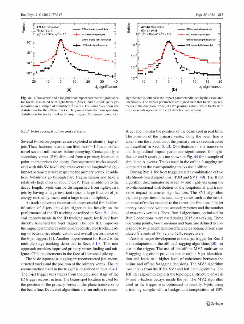
Eur. Phys. J. C (2017) 77 :317 Page 35 of 53 317
signi cance0d
20− 10− 0 10 20 30 40
Ent
ries
4−10
3−10
2−10
1−10
1Offline tracks b-quark jets
HLT tracks b-quark jets
O ine tracks light- avour jet
HLT tracks light- avour jets
ATLAS Simulationt=13 TeV, ts
| < 2.5jetη> 40 GeV, |jet
Tp
(a)signi cance0z
10− 5− 0 5 10 15 20
Ent
ries
4−10
3−10
2−10
1−10
1
Offline tracks b-quark jets
HLT tracks b-quark jets
O ine tracks light- avour jet
HLT tracks light- avour jets
ATLAS Simulationt=13 TeV, ts
| < 2.5jetη> 40 GeV, |jet
Tp
(b)
Fig. 44 aTransverse and b longitudinal impact parameter significancefor tracks associated with light-flavour (black) and b-quark (red) jetsmeasured in a sample of simulated t t events. The solid lines show thedistribution for the offline tracks. The points show the correspondingdistribution for tracks used in the b-jet trigger. The impact parameter
significance is defined as the impact parameter divided by the associateduncertainty. The impact parameters are signed such that track displace-ments in the direction of the jet have positive values, while tracks withdisplacements opposite of the jet direction are negative
6.7.1 b-Jet reconstruction and selection
Several b-hadron properties are exploited to identify (tag) b-jets. The b-hadrons have a mean lifetime of ∼1.5 ps and oftentravel several millimetres before decaying. Consequently, asecondary vertex (SV) displaced from a primary interactionpoint characterises the decay. Reconstructed tracks associ-ated with this SV have large transverse and longitudinal (z0)impact parameters with respect to the primary vertex. In addi-tion, b-hadrons go through hard fragmentation and have arelatively high mass of about 5 GeV. Thus, in addition to thedecay length, b-jets can be distinguished from light-quarkjets by having a large invariant mass, a large fraction of jetenergy carried by tracks and a large track multiplicity.
As track and vertex reconstruction are crucial for the iden-tification of b-jets, the b-jet trigger relies heavily on theperformance of the ID tracking described in Sect. 5.1. Sev-eral improvements in the ID tracking made for Run 2 havedirectly benefited the b-jet trigger. The new IBL improvesthe impact parameter resolution of reconstructed tracks, lead-ing to better b-jet identification and overall performance ofthe b-jet triggers [7]. Another improvement for Run 2 is themultiple-stage tracking described in Sect. 5.1.3. This newapproach provides improved primary vertex finding and mit-igates CPU requirements in the face of increased pile-up.
The basic inputs to b-tagging are reconstructed jets, recon-structed tracks and the position of the primary vertex. The jetreconstruction used in the trigger is described in Sect. 6.4.1.The b-jet trigger uses tracks from the precision stage of theID trigger reconstruction. The beam-spot location is used forthe position of the primary vertex in the plane transverse tothe beam line. Dedicated algorithms are run online to recon-
struct and monitor the position of the beam spot in real time.The position of the primary vertex along the beam line istaken from the z position of the primary vertex reconstructedas described in Sect. 5.1.3. Distributions of the transverseand longitudinal impact parameter significances for light-flavour and b-quark jets are shown in Fig. 44 for a sample ofsimulated t t events. Tracks used in the online b-tagging arecompared to the corresponding tracks used offline.
During Run 1, the b-jet triggers used a combination of twolikelihood-based algorithms, IP3D and SV1 [49]. The IP3Dalgorithm discriminates between b- and light-jets using thetwo-dimensional distribution of the longitudinal and trans-verse impact parameter significances. The SV1 algorithmexploits properties of the secondary vertex such as the invari-ant mass of tracks matched to the vertex, the fraction of the jetenergy associated with the secondary vertex and the numberof two-track vertices. These Run 1 algorithms, optimised forRun 2 conditions, were used during 2015 data-taking. Threeoperating points, loose, medium and tight, are defined to cor-respond to b-jet identification efficiencies obtained from sim-ulated t t events of 79, 72 and 62%, respectively.
Another major development in the b-jet trigger for Run 2is the adaptation of the offline b-tagging algorithms [50] foruse in the trigger. The use of the offline MV2 multivariateb-tagging algorithm provides better online b-jet identifica-tion and leads to a higher level of coherence between theonline and offline b-tagging decisions. The MV2 algorithmuses inputs from the IP3D, SV1 and JetFitter algorithms. TheJetFitter algorithm exploits the topological structure of weakb- and c-hadron decays inside the jet. The MV2 algorithmused in the trigger was optimised to identify b-jets usinga training sample with a background composition of 80%
123

317 Page 36 of 53 Eur. Phys. J. C (2017) 77 :317
b-jet efficiency [%]
40 50 60 70 80 90 100
Ligh
t jet
rej
ectio
n
1
10
210
310
410
MV2c20
IP3D+SV1
2012 operatingpoints (IP3D+SV1)
ATLAS Simulationtt simulations = 13 TeV
> 55 GeV, |η|<2.5T
Jet p
Fig. 45 The expected performance of the MV2c20 trigger tagger (solidblack line) in terms of light-jet rejection is shown together with theexpected performance of the IP3D+SV1 trigger tagger in Run 2 (dashedblue line) and its actual performance achieved during Run 1 (red stars)
(20%) light- (c-) jets and is referred to as MV2c20. Operat-ing points analogous to loose,medium and tight were definedfor MV2c20 and give light-flavour rejections similar to thecorresponding operating points of the Run 1 b-tagging algo-rithm. Triggers utilising the MV2c20 b-tagging algorithmwere run in 2015 for commissioning purposes. MV2c20 isthe baseline b-tagging algorithm for 2016. Figure 45 showsthe expected performance of the MV2c20 and the IP3D+SV1trigger taggers in Run 2 compared to the actual performanceof the IP3D+SV1 tagger that was achieved during Run 1.
Figure 46 shows the efficiency of the online b-taggingas a function of jet pT for the three operating points. Theefficiencies are calculated in a pure sample of b-jets fromfully leptonic t t decays and are computed with respect tojets identified by the 70% working point of the MV2c20algorithm. Events used in the efficiency calculation requirean online jet with pT greater than 40 GeV. A significantgain in trigger efficiency is seen when moving to the MV2b-tagging algorithms.
6.7.2 b-Jet trigger menu and rates
Several b-jet triggers have been implemented with differ-ent combinations of jets and b-tagged jets, using differentpT thresholds and b-tagging operating points. The operatingpoints, thresholds and multiplicities, for several of the pri-mary b-jet triggers are listed in Table 1. The jet multiplicitiesvary between one and four, with up to two b-tagged jets. Theb-jet triggers are typically seeded at L1 using either a singlejet with ET > 100 GeV or three jets with ET > 25 GeV andpseudorapidity |η| < 2.5. Rates of various b-jet triggers as afunction of luminosity are shown in Fig. 47.
[GeV]T
Jet p50 100 150 200 250 300 350 400T
rigge
r ef
ficie
ncy
w.r
.t. 7
0% o
fflin
e b-
tag
0
0.2
0.4
0.6
0.8
1
1.2
MV2 Tagging Algorithm
IP3D+SV1 Tagging Algorithm
Loose Medium Tight
ATLAS-1=13 TeV, 3.2 fbs | < 2.5jetη> 40 GeV, |jet
Tp
Fig. 46 b-jet trigger efficiency as a function of jet pT for the loose(blue), medium (black) and tight (red) operating points. The opensquares show the trigger efficiency using the IP3D+SV1 b-taggingalgorithm. The closed circles show the trigger efficiency for the cor-responding MV2 b-tagging algorithm working points. The efficienciesare measured in a pure sample of b-jets selected in t t events and arecomputed with respect to jets identified by the 70% working point ofthe offline MV2c20 b-tagging algorithm
]-1s-2cm33Inst. luminosity [10
1 2 3 4
Rat
e [H
z]
0
5
10
15
20
25
30
35
= 13 TeVsData (2015) ATLASHLT_j300_blooseHLT_j225_blooseHLT_2j70_bmedium_j70HLT_2j70_btight_j70
Fig. 47 Rates of b-jet triggers as a function of the instantaneous lumi-nosity
The benefit of exploiting b-tagging in the HLT can be seenby comparing the thresholds used in jet triggers with andwithout b-tagging. The threshold for the lowest unprescaledsingle-jet trigger without b-tagging is 360 GeV. A looserequirement in the trigger allows this threshold to be low-ered to 225 GeV. For the four-jet trigger, 85 GeV thresholdsare used when no b-tagging is applied. Requiring two jetsto satisfy the tight b-tagging requirement allows the four-jetthreshold to be lowered to 35 GeV.
123

Eur. Phys. J. C (2017) 77 :317 Page 37 of 53 317
]-1s-2cm33Instantaneous luminosity [100 1 2 3 4 5
Rat
e [k
Hz]
0
5
10
15
20
25
30ATLAS
-1= 13 TeV, 3.2 fbsL1_2MU4L1_MU6_2MU4L1_2MU6
(a)
]-1s-2cm33Instantaneous luminosity [100 1 2 3 4 5
Rat
e [H
z]
0
10
20
30
40
50
60
70
80ATLAS
-1= 13 TeV, 3.2 fbsHLT_2mu4_bJpsimumuHLT_mu6_mu4_bJpsimumuHLT_2mu6_bJpsimumu
HLT_mu6_mu4_bBmumuHLT_mu6_mu4_bUpsimumuHLT_mu6_mu4_bBmumuxv2
(b)
Fig. 48 Trigger rates for a low-pT dimuon L1 triggers with variousmuon pT thresholds and b primary HLT B-physics triggers as a func-tion of instantaneous luminosity. b Shows triggers requiring two muonsto pass various pT thresholds, to have an invariant mass within the J/ψmass window, and to form a good vertex (full markers); also shown aretriggers requiring two muons with pT > 6 and 4 GeV and either having
an invariant mass in a different window (B0(s), ϒ(1, 2, 3S)) or forming a
B → μμX candidate after combination with additional tracks found inID (open markers). As L1_2MU4 was prescaled at luminosities above4 × 1033 cm−2s−1, the rate of 2mu4_bJpsimumu seeded from thisL1 trigger drops above that luminosity
6.8 B-physics
The trigger selection of events for B-physics analyses isprimarily based on the identification of b-hadrons throughdecays including a muon pair in the final state. Examples aredecays with charmonium, B → J/ψ(→ μμ)X , rare decaysB0
(s) → μμ, and semileptonic B → μμX . Decays of promptcharmonium and bottomonium are also identified throughtheir dimuon decays, and are therefore similar to b-hadrondecays, apart from the lack of measurable displacement fromthe pp interaction point.
6.8.1 B-physics reconstruction and selection
The primary suite of triggers require two muons at L1. Theirrate is substantially reduced compared to single-muon L1triggers. However, this results in inefficiencies at high trans-verse momentum, where the opening angle of the two muonsbecomes small for low-mass resonances, and the granular-ity at L1 is not sufficient to form separate RoIs. At theHLT, muons are reconstructed using the same algorithms asdescribed in Sect. 5.3 with the additional requirement thatthe two muons should have opposite charges and form agood vertex (where the fit is performed using the ID trackparameters) within a certain invariant mass window. Theprimary triggers use three dimuon mass windows: 2.5 to4.3 GeV intended for the selection of J/ψ and ψ(2S) decaysinto muon pairs (including charmonia produced in b-hadrondecays), 4.0 to 8.5 GeV for B0
(s) → μμ decays, and 8 to12 GeV for ϒ(1, 2, 3S) → μμ decays. These invariant mass
selections are indicated by the bJpsimumu, bBmumu andbUpsimumu suffixes in the trigger names, respectively.
Additional primary and supporting triggers are also imple-mented. Triggers using a single L1 muon RoI with an addi-tional track found at the HLT do not have similar openingangle issues, but suffer from high rates and run with highprescale factors. These combined muon triggers are, how-ever, essential components in data-driven estimates of thedimuon trigger efficiencies. Triggers requiring three muonsat L1 help to maintain the lowest muon pT thresholds forcertain event signatures with a likely presence of a thirdmuon. Finally, for selecting semileptonic decays, such asB0 → μμK ∗0(→ K+π−), searches for additional IDtracks and a combined vertex fit are performed assuminga few exclusive decay hypotheses. This reduces the rate withrespect to a simple dimuon vertex selection thus allowingthe dimuon mass window to be widened to the full kinemat-ically allowed range. The corresponding trigger names usethe bBmumuxv2 suffix.
6.8.2 B-physics trigger menu and rates
Dimuon trigger rate restrictions at L1 define the lowest muontransverse momentum thresholds for primary B-physics trig-gers in 2015 data-taking. HLT triggers using L1_2MU4wereunprescaled up to a luminosity of 4×1033 cm−2 s−1. Abovethis, triggers seeded from L1_MU6_2MU4,6 which requires
6 L1 muon thresholds are inclusive, i.e. L1_MU6_2MU4 is a dimuontrigger.
123
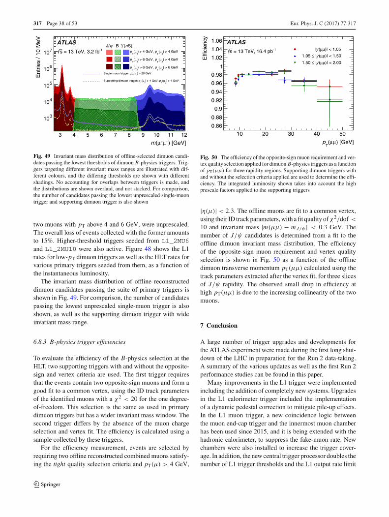
317 Page 38 of 53 Eur. Phys. J. C (2017) 77 :317
) [GeV]−μ+μ(m3 4 5 6 7 8 9 10 11 12
Ent
ries
/ 10
MeV
310
410
510
610
710ψJ/ B S)n(ϒ
) > 4 GeV2
μ(T
p) > 4 GeV, 1
μ(T
p
) > 4 GeV2
μ(T
p) > 6 GeV, 1
μ(T
p
) > 6 GeV2
μ(T
p) > 6 GeV, 1
μ(T
p
) > 20 GeV1
μ(T
pSingle muon trigger:
) > 4 GeV2
μ(T
p) > 4 GeV, 1
μ(T
pSupporting dimuon trigger:
ATLAS-1 = 13 TeV, 3.2 fbs
Fig. 49 Invariant mass distribution of offline-selected dimuon candi-dates passing the lowest thresholds of dimuon B-physics triggers. Trig-gers targeting different invariant mass ranges are illustrated with dif-ferent colours, and the differing thresholds are shown with differentshadings. No accounting for overlaps between triggers is made, andthe distributions are shown overlaid, and not stacked. For comparison,the number of candidates passing the lowest unprescaled single-muontrigger and supporting dimuon trigger is also shown
two muons with pT above 4 and 6 GeV, were unprescaled.The overall loss of events collected with the former amountsto 15%. Higher-threshold triggers seeded from L1_2MU6and L1_2MU10 were also active. Figure 48 shows the L1rates for low-pT dimuon triggers as well as the HLT rates forvarious primary triggers seeded from them, as a function ofthe instantaneous luminosity.
The invariant mass distribution of offline reconstructeddimuon candidates passing the suite of primary triggers isshown in Fig. 49. For comparison, the number of candidatespassing the lowest unprescaled single-muon trigger is alsoshown, as well as the supporting dimuon trigger with wideinvariant mass range.
6.8.3 B-physics trigger efficiencies
To evaluate the efficiency of the B-physics selection at theHLT, two supporting triggers with and without the opposite-sign and vertex criteria are used. The first trigger requiresthat the events contain two opposite-sign muons and form agood fit to a common vertex, using the ID track parametersof the identified muons with a χ2 < 20 for the one degree-of-freedom. This selection is the same as used in primarydimuon triggers but has a wider invariant mass window. Thesecond trigger differs by the absence of the muon chargeselection and vertex fit. The efficiency is calculated using asample collected by these triggers.
For the efficiency measurement, events are selected byrequiring two offline reconstructed combined muons satisfy-ing the tight quality selection criteria and pT(μ) > 4 GeV,
) [GeV]μμ(T
p
10 20 30 40 50
Effi
cien
cy
0.86
0.88
0.9
0.92
0.94
0.96
0.98
1
1.02
1.04
1.06)| < 1.05μμ(y |
)| < 1.50μμ(y |≤1.05
)| < 2.00μμ(y |≤1.50
ATLAS-1 = 13 TeV, 16.4 pbs
Fig. 50 The efficiency of the opposite-sign muon requirement and ver-tex quality selection applied for dimuon B-physics triggers as a functionof pT(μμ) for three rapidity regions. Supporting dimuon triggers withand without the selection criteria applied are used to determine the effi-ciency. The integrated luminosity shown takes into account the highprescale factors applied to the supporting triggers
|η(μ)| < 2.3. The offline muons are fit to a common vertex,using their ID track parameters, with a fit quality of χ2/dof <
10 and invariant mass |m(μμ) − mJ/ψ | < 0.3 GeV. Thenumber of J/ψ candidates is determined from a fit to theoffline dimuon invariant mass distribution. The efficiencyof the opposite-sign muon requirement and vertex qualityselection is shown in Fig. 50 as a function of the offlinedimuon transverse momentum pT(μμ) calculated using thetrack parameters extracted after the vertex fit, for three slicesof J/ψ rapidity. The observed small drop in efficiency athigh pT(μμ) is due to the increasing collinearity of the twomuons.
7 Conclusion
A large number of trigger upgrades and developments forthe ATLAS experiment were made during the first long shut-down of the LHC in preparation for the Run 2 data-taking.A summary of the various updates as well as the first Run 2performance studies can be found in this paper.
Many improvements in the L1 trigger were implementedincluding the addition of completely new systems. Upgradesin the L1 calorimeter trigger included the implementationof a dynamic pedestal correction to mitigate pile-up effects.In the L1 muon trigger, a new coincidence logic betweenthe muon end-cap trigger and the innermost muon chamberhas been used since 2015, and it is being extended with thehadronic calorimeter, to suppress the fake-muon rate. Newchambers were also installed to increase the trigger cover-age. In addition, the new central trigger processor doubles thenumber of L1 trigger thresholds and the L1 output rate limit
123

Eur. Phys. J. C (2017) 77 :317 Page 39 of 53 317
has increased from 70 to 100 kHz. Furthermore, a new topo-logical processor was installed and is being commissioned.A new HLT architecture was developed to unify the Level-2and Event Filter scheme used in Run 1, improving the flex-ibility of the system. The HLT software was also upgraded,making the algorithms and selections closer to the offlinereconstruction to maximise the efficiency, and making use ofthe newly installed systems such as the innermost pixel layerIBL.
The trigger menu was revisited and redesigned to copewith the greater rates due to the higher centre-of-mass energyand increasing instantaneous luminosity. The different trig-ger signatures were set up according to the physics needs,considering different luminosity scenarios. The ATLAS trig-ger system was successfully commissioned with the first dataacquired at 13 TeV. First performance studies of the differ-ent trigger signatures and trigger efficiencies with respect tothe offline quantities are presented using the 13 TeV proton–proton collision data with a 25 ns bunch separation collectedduring 2015.
Acknowledgements We thank CERN for the very successful oper-ation of the LHC, as well as the support staff from our institutionswithout whom ATLAS could not be operated efficiently. We acknowl-edge the support of ANPCyT, Argentina; YerPhI, Armenia; ARC,Australia; BMWFW and FWF, Austria; ANAS, Azerbaijan; SSTC,Belarus; CNPq and FAPESP, Brazil; NSERC, NRC and CFI, Canada;CERN; CONICYT, Chile; CAS, MOST and NSFC, China; COLCIEN-CIAS, Colombia; MSMT CR, MPO CR and VSC CR, Czech Repub-lic; DNRF and DNSRC, Denmark; IN2P3-CNRS, CEA-DSM/IRFU,France; SRNSF, Georgia; BMBF, HGF, and MPG, Germany; GSRT,Greece; RGC, Hong Kong SAR, China; ISF, I-CORE and BenoziyoCenter, Israel; INFN, Italy; MEXT and JSPS, Japan; CNRST, Morocco;NWO, Netherlands; RCN, Norway; MNiSW and NCN, Poland; FCT,Portugal; MNE/IFA, Romania; MES of Russia and NRC KI, RussianFederation; JINR; MESTD, Serbia; MSSR, Slovakia; ARRS and MIZŠ,Slovenia; DST/NRF, South Africa; MINECO, Spain; SRC and Wal-lenberg Foundation, Sweden; SERI, SNSF and Cantons of Bern andGeneva, Switzerland; MOST, Taiwan; TAEK, Turkey; STFC, UnitedKingdom; DOE and NSF, USA. In addition, individual groups andmembers have received support from BCKDF, the Canada Council,CANARIE, CRC, Compute Canada, FQRNT, and the Ontario Inno-vation Trust, Canada; EPLANET, ERC, ERDF, FP7, Horizon 2020and Marie Skłodowska-Curie Actions, European Union; Investisse-ments d’Avenir Labex and Idex, ANR, Région Auvergne and FondationPartager le Savoir, France; DFG and AvH Foundation, Germany; Herak-leitos, Thales and Aristeia programmes co-financed by EU-ESF and theGreek NSRF; BSF, GIF and Minerva, Israel; BRF, Norway; CERCAProgramme Generalitat de Catalunya, Generalitat Valenciana, Spain;the Royal Society and Leverhulme Trust, United Kingdom. The crucialcomputing support from all WLCG partners is acknowledged grate-fully, in particular from CERN, the ATLAS Tier-1 facilities at TRIUMF(Canada), NDGF (Denmark, Norway, Sweden), CC-IN2P3 (France),KIT/GridKA (Germany), INFN-CNAF (Italy), NL-T1 (Netherlands),PIC (Spain), ASGC (Taiwan), RAL (UK) and BNL (USA), the Tier-2facilities worldwide and large non-WLCG resource providers. Majorcontributors of computing resources are listed in Ref. [51].
Open Access This article is distributed under the terms of the CreativeCommons Attribution 4.0 International License (http://creativecommons.org/licenses/by/4.0/), which permits unrestricted use, distribution,
and reproduction in any medium, provided you give appropriate creditto the original author(s) and the source, provide a link to the CreativeCommons license, and indicate if changes were made.Funded by SCOAP3.
References
1. ATLAS Collaboration, Performance of the ATLAS trigger sys-tem in 2010. Eur. Phys. J. C 72, 1849 (2012). doi:10.1140/epjc/s10052-011-1849-1. arXiv:1110.1530 [hep-ex]
2. ATLAS Collaboration, Performance of the ATLAS electron andphoton trigger in pp collisions at
√s = 7 TeV in 2011. ATLAS-
CONF-2012-048 (2012). http://cds.cern.ch/record/14500893. ATLAS Collaboration, Performance of the ATLAS muon trigger
in pp collisions at√s = 8 TeV. Eur. Phys. J. C 75, 120 (2015).
doi:10.1140/epjc/s10052-015-3325-9. arXiv:1408.3179 [hep-ex]4. ATLAS Collaboration, Identification and energy calibration of
hadronically decaying tau leptons with the ATLAS experiment inpp collisions at
√s = 8 TeV. Eur. Phys. J. C 75, 303 (2015).
doi:10.1140/epjc/s10052-015-3500-z. arXiv:1412.7086 [hep-ex]5. ATLAS Collaboration, The performance of the jet trigger for the
ATLAS detector during 2011 data taking. Eur. Phys. J. C 76, 526(2016). doi:10.1140/epjc/s10052-016-4325-0. arXiv:1606.07759[hep-ex]
6. ATLAS Collaboration, The ATLAS experiment at the CERN largehadron collider. JINST 3, S08003 (2008). doi:10.1088/1748-0221/3/08/S08003
7. ATLAS Collaboration, ATLAS insertable B-layer technicaldesign report. ATLAS-TDR-19 (2010). http://cds.cern.ch/record/1291633 [ATLAS insertable B-layer technical design report adden-dum. ATLAS-TDR-19-ADD-1 (2012). http://cds.cern.ch/record/1451888]
8. T. Sjöstrand, S. Mrenna, P.Z. Skands, A brief introductionto PYTHIA 8.1. Comput. Phys. Commun. 178, 852 (2008).arXiv:0710.3820 [hep-ph]
9. R.D. Ball et al., Parton distributions with LHC data. Nucl. Phys. B867, 244 (2013). arXiv:1207.1303 [hep-ph]
10. P. Nason, A new method for combining NLO QCD withshower Monte Carlo algorithms. JHEP 11, 040 (2004).arXiv:hep-ph/0409146 [hep-ph]
11. S. Frixione, P. Nason, C. Oleari, Matching NLO QCD computationswith parton shower simulations: the POWHEG method. JHEP 11,070 (2007). arXiv:0709.2092 [hep-ph]
12. S. Alioli et al., A general framework for implementing NLO cal-culations in shower Monte Carlo programs: the POWHEG BOX.JHEP 06, 043 (2010). arXiv:1002.2581 [hep-ph]
13. H.-L. Lai et al., New parton distributions for collider physics. Phys.Rev. D 82, 074024 (2010). arXiv:1007.2241 [hep-ph]
14. T. Sjöstrand, S. Mrenna, P.Z. Skands, PYTHIA 6.4 physics andmanual. JHEP 0605, 026 (2006). arXiv:hep-ph/0603175 [hep-ph]
15. J. Pumplin et al., New generation of parton distributions withuncertainties from global QCD analysis. JHEP 0207, 012 (2002).arXiv:hep-ph/0201195 [hep-ph]
16. ATLAS Collaboration, The ATLAS data acquisition and high leveltrigger system. JINST 11, P06008 (2016). doi:10.1088/1748-0221/11/06/P06008
17. ATLAS Collaboration, Technical design report for the phase-Iupgrade of the ATLAS TDAQ system. ATLAS-TDR-023 (2013).http://cdsweb.cern.ch/record/1602235
18. ATLAS Collaboration, Fast TracKer (FTK) technical design report.ATLAS-TDR-021 (2013). http://cdsweb.cern.ch/record/1552953
19. R. Achenbach et al., The ATLAS level-1 calorimeter trigger. JINST3, P03001 (2008). doi:10.1088/1748-0221/3/03/P03001
123
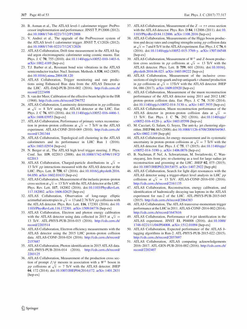
317 Page 40 of 53 Eur. Phys. J. C (2017) 77 :317
20. B. Asman et al., The ATLAS level-1 calorimeter trigger: PrePro-cessor implementation and performance. JINST 7, P12008 (2012).doi:10.1088/1748-0221/7/12/P12008
21. V. Andrei et al., The upgrade of the PreProcessor system ofthe ATLAS level-1 calorimeter trigger. JINST 7, C12026 (2012).doi:10.1088/1748-0221/7/12/C12026
22. ATLAS Collaboration, Drift time measurement in the ATLAS liq-uid argon electromagnetic calorimeter using cosmic muons. Eur.Phys. J. C 70, 755 (2010). doi:10.1140/epjc/s10052-010-1403-6.arXiv:1002.4189 [hep-ex]
23. T.J. Barber et al., Resonant bond wire vibrations in the ATLASsemiconductor tracker. Nucl. Instrum. Methods A 538, 442 (2005).doi:10.1016/j.nima.2004.08.120
24. ATLAS Collaboration, Trigger monitoring and rate predic-tions using Enhanced Bias data from the ATLAS Detector atthe LHC. ATL-DAQ-PUB-2016-002 (2016). http://cds.cern.ch/record/2223498
25. S. van der Meer, Calibration of the effective beam height in the ISR(1968). http://cds.cern.ch/record/296752
26. ATLAS Collaboration, Luminosity determination in pp collisionsat
√s = 8 TeV using the ATLAS detector at the LHC. Eur.
Phys. J. C 76, 653 (2016). doi:10.1140/epjc/s10052-016-4466-1.arXiv:1608.03953 [hep-ex]
27. ATLAS Collaboration, Performance of primary vertex reconstruc-tion in proton–proton collisions at
√s = 7 TeV in the ATLAS
experiment. ATLAS-CONF-2010-069 (2010). http://cds.cern.ch/record/1281344
28. ATLAS Collaboration, Topological cell clustering in the ATLAScalorimeters and its performance in LHC Run 1 (2016).arXiv:1603.02934 [hep-ex]
29. N. Berger et al., The ATLAS high level trigger steering. J. Phys.Conf. Ser. 119, 022013 (2008). doi:10.1088/1742-6596/119/2/022013
30. ATLAS Collaboration, Charged-particle distributions in√s =
13 TeV pp interactions measured with the ATLAS detector at theLHC. Phys. Lett. B 758, 67 (2016). doi:10.1016/j.physletb.2016.04.050. arXiv:1602.01633 [hep-ex]
31. ATLAS Collaboration, Measurement of the inelastic proton–protoncross section at
√s = 13 TeV with the ATLAS detector at the LHC.
Phys. Rev. Lett. 117, 182002 (2016). doi:10.1103/PhysRevLett.117.182002. arXiv:1606.02625 [hep-ex]
32. ATLAS Collaboration, Observation of long-range ellipticazimuthal anisotropies in
√s = 13 and 2.76 TeV pp collisions with
the ATLAS detector. Phys. Rev. Lett. 116, 172301 (2016). doi:10.1103/PhysRevLett.116.172301. arXiv:1509.04776 [hep-ex]
33. ATLAS Collaboration, Electron and photon energy calibrationwith the ATLAS detector using data collected in 2015 at
√s =
13 TeV. ATL-PHYS-PUB-2016-015 (2016). http://cds.cern.ch/record/2203514
34. ATLAS Collaboration, Electron efficiency measurements with theATLAS detector using the 2015 LHC proton–proton collisiondata. ATLAS-CONF-2016-024 (2016). http://cds.cern.ch/record/2157687
35. ATLAS Collaboration, Photon identification in 2015 ATLAS data.ATL-PHYS-PUB-2016-014 (2016). http://cds.cern.ch/record/2203125
36. ATLAS Collaboration, Measurement of the production cross sec-tion of prompt J/ψ mesons in association with a W± boson inpp collisions at
√s = 7 TeV with the ATLAS detector. JHEP
04, 172 (2014). doi:10.1007/JHEP04(2014)172. arXiv:1401.2831[hep-ex]
37. ATLAS Collaboration, Measurement of the Z → ττ cross sectionwith the ATLAS detector. Phys. Rev. D 84, 112006 (2011). doi:10.1103/PhysRevD.84.112006. arXiv:1108.2016 [hep-ex]
38. ATLAS Collaboration, Measurements of the Higgs boson produc-tion and decay rates and coupling strengths using pp collision dataat
√s = 7 and 8 TeV in the ATLAS experiment. Eur. Phys. J. C76, 6
(2016). doi:10.1140/epjc/s10052-015-3769-y. arXiv:1507.04548[hep-ex]
39. ATLAS Collaboration, Measurement of W± and Z -boson produc-tion cross sections in pp collisions at
√s = 13 TeV with the
ATLAS detector. Phys. Lett. B 759, 601 (2016). doi:10.1016/j.physletb.2016.06.023. arXiv:1603.09222 [hep-ex]
40. ATLAS Collaboration, Measurement of the inclusive cross-sections of single top-quark and top-antiquark t-channel productionin pp collisions at
√s = 13TeV with the ATLAS detector. JHEP
04, 086 (2017). arXiv:1609.03920 [hep-ex]41. ATLAS Collaboration, Measurement of the muon reconstruction
performance of the ATLAS detector using 2011 and 2012 LHCproton–proton collision data. Eur. Phys. J. C 74, 3130 (2014).doi:10.1140/epjc/s10052-014-3130-x. arXiv:1407.3935 [hep-ex]
42. ATLAS Collaboration, Muon reconstruction performance of theATLAS detector in proton–proton collision data at
√s =
13 TeV. Eur. Phys. J. C 76, 292 (2016). doi:10.1140/epjc/s10052-016-4120-y. arXiv:1603.05598 [hep-ex]
43. M. Cacciari, G. Salam, G. Soyez, The anti-kT jet clustering algo-rithm. JHEP 04, 063 (2008). doi:10.1088/1126-6708/2008/04/063.arXiv:0802.1189 [hep-ph]
44. ATLAS Collaboration, Jet energy measurement and its systematicuncertainty in proton–proton collisions at
√s = 7 TeV with the
ATLAS detector. Eur. Phys. J. C 75, 17 (2015). doi:10.1140/epjc/s10052-014-3190-y. arXiv:1406.0076 [hep-ex]
45. B. Nachman, P. Nef, A. Schwartzman, M. Swiatlowski, C. Wan-otayaroj, Jets from jets: re-clustering as a tool for large radius jetreconstruction and grooming at the LHC. JHEP 02, 075 (2015).doi:10.1007/JHEP02(2015)075. arXiv:1407.2922 [hep-ph]
46. ATLAS Collaboration, Search for light dijet resonances with theATLAS detector using a trigger-object level analysis in LHC ppcollisions at
√s = 13 TeV. ATLAS-CONF-2016-030 (2016).
http://cds.cern.ch/record/216113547. ATLAS Collaboration, Reconstruction, energy calibration, and
identification of hadronically decaying tau leptons in the ATLASexperiment for run-2 of the LHC. ATL-PHYS-PUB-2015-045(2015). http://cds.cern.ch/record/2064383
48. ATLAS Collaboration, The ATLAS transverse-momentum triggerperformance at the LHC in 2011. ATLAS-CONF-2014-002 (2014).http://cds.cern.ch/record/1647616
49. ATLAS Collaboration, Performance of b-jet identification in theATLAS experiment. JINST 11, P04008 (2016). doi:10.1088/1748-0221/11/04/P04008. arXiv:1512.01094 [hep-ex]
50. ATLAS Collaboration, Expected performance of the ATLAS b-tagging algorithms in Run-2. ATL-PHYS-PUB-2015-022 (2015).http://cds.cern.ch/record/2037697
51. ATLAS Collaboration, ATLAS computing acknowledgements2016–2017. ATL-GEN-PUB-2016-002 (2016). http://cds.cern.ch/record/2202407
123
Eur. Phys. J. C (2017) 77 :317 Page 41 of 53 317
ATLAS Collaboration
M. Aaboud137d, G. Aad88, B. Abbott115, J. Abdallah8, O. Abdinov12, B. Abeloos119, R. Aben109, O. S. AbouZeid139,N. L. Abraham151, H. Abramowicz155, H. Abreu154, R. Abreu118, Y. Abulaiti148a,148b, B. S. Acharya167a,167b,a, S. Adachi157,L. Adamczyk41a, D. L. Adams27, J. Adelman110, S. Adomeit102, T. Adye133, A. A. Affolder77, T. Agatonovic-Jovin14,J. A. Aguilar-Saavedra128a,128f, S. P. Ahlen24, F. Ahmadov68,b, G. Aielli135a,135b, H. Akerstedt148a,148b,T. P. A. Åkesson84, A. V. Akimov98, G. L. Alberghi22a,22b, J. Albert172, S. Albrand58, M. J. Alconada Verzini74,M. Aleksa32, I. N. Aleksandrov68, C. Alexa28b, G. Alexander155, T. Alexopoulos10, M. Alhroob115, B. Ali130,M. Aliev76a,76b, G. Alimonti94a, J. Alison33, S. P. Alkire38, B. M. M. Allbrooke151, B. W. Allen118, P. P. Allport19,A. Aloisio106a,106b, A. Alonso39, F. Alonso74, C. Alpigiani140, A. A. Alshehri56, M. Alstaty88, B. Alvarez Gonzalez32,D. Álvarez Piqueras170, M. G. Alviggi106a,106b, B. T. Amadio16, Y. Amaral Coutinho26a, C. Amelung25, D. Amidei92,S. P. Amor Dos Santos128a,128c, A. Amorim128a,128b, S. Amoroso32, G. Amundsen25, C. Anastopoulos141, L. S. Ancu52,N. Andari19, T. Andeen11, C. F. Anders60b, G. Anders32, J. K. Anders77, K. J. Anderson33, A. Andreazza94a,94b,V. Andrei60a, S. Angelidakis9, I. Angelozzi109, A. Angerami38, F. Anghinolfi32, A. V. Anisenkov111,c, N. Anjos13,A. Annovi126a,126b, C. Antel60a, M. Antonelli50, A. Antonov100,*, D. J. Antrim166, F. Anulli134a, M. Aoki69,L. Aperio Bella19, G. Arabidze93, Y. Arai69, J. P. Araque128a, A. T. H. Arce48, F. A. Arduh74, J.-F. Arguin97,S. Argyropoulos66, M. Arik20a, A. J. Armbruster145, L. J. Armitage79, O. Arnaez32, H. Arnold51, M. Arratia30,O. Arslan23, A. Artamonov99, G. Artoni122, S. Artz86, S. Asai157, N. Asbah45, A. Ashkenazi155, B. Åsman148a,148b,L. Asquith151, K. Assamagan27, R. Astalos146a, M. Atkinson169, N. B. Atlay143, K. Augsten130, G. Avolio32, B. Axen16,M. K. Ayoub119, G. Azuelos97,d, M. A. Baak32, A. E. Baas60a, M. J. Baca19, H. Bachacou138, K. Bachas76a,76b,M. Backes122, M. Backhaus32, P. Bagiacchi134a,134b, P. Bagnaia134a,134b, Y. Bai35a, J. T. Baines133, M. Bajic39,O. K. Baker179, E. M. Baldin111,c, P. Balek175, T. Balestri150, F. Balli138, W. K. Balunas124, E. Banas42, Sw. Banerjee176,e,A. A. E. Bannoura178, L. Barak32, E. L. Barberio91, D. Barberis53a,53b, M. Barbero88, T. Barillari103, M.-S. Barisits32,T. Barklow145, N. Barlow30, S. L. Barnes87, B. M. Barnett133, R. M. Barnett16, Z. Barnovska-Blenessy36a, A. Baroncelli136a,G. Barone25, A. J. Barr122, L. Barranco Navarro170, F. Barreiro85, J. Barreiro Guimarães da Costa35a, R. Bartoldus145,A. E. Barton75, P. Bartos146a, A. Basalaev125, A. Bassalat119,f, R. L. Bates56, S. J. Batista161, J. R. Batley30, M. Battaglia139,M. Bauce134a,134b, F. Bauer138, H. S. Bawa145,g, J. B. Beacham113, M. D. Beattie75, T. Beau83, P. H. Beauchemin165,P. Bechtle23, H. P. Beck18,h, K. Becker122, M. Becker86, M. Beckingham173, C. Becot112, A. J. Beddall20d, A. Beddall20b,V. A. Bednyakov68, M. Bedognetti109, C. P. Bee150, L. J. Beemster109, T. A. Beermann32, M. Begel27, J. K. Behr45,A. S. Bell81, G. Bella155, L. Bellagamba22a, A. Bellerive31, M. Bellomo89, K. Belotskiy100, O. Beltramello32,N. L. Belyaev100, O. Benary155,*, D. Benchekroun137a, M. Bender102, K. Bendtz148a,148b, N. Benekos10, Y. Benhammou155,E. Benhar Noccioli179, J. Benitez66, D. P. Benjamin48, J. R. Bensinger25, S. Bentvelsen109, L. Beresford122, M. Beretta50,D. Berge109, E. Bergeaas Kuutmann168, N. Berger5, J. Beringer16, S. Berlendis58, N. R. Bernard89, C. Bernius112,F. U. Bernlochner23, T. Berry80, P. Berta131, C. Bertella86, G. Bertoli148a,148b, F. Bertolucci126a,126b, I. A. Bertram75,C. Bertsche45, D. Bertsche115, G. J. Besjes39, O. Bessidskaia Bylund148a,148b, M. Bessner45, N. Besson138, C. Betancourt51,A. Bethani58, S. Bethke103, A. J. Bevan79, R. M. Bianchi127, M. Bianco32, O. Biebel102, D. Biedermann17, R. Bielski87,N. V. Biesuz126a,126b, M. Biglietti136a, J. Bilbao De Mendizabal52, T. R. V. Billoud97, H. Bilokon50, M. Bindi57,A. Bingul20b, C. Bini134a,134b, S. Biondi22a,22b, T. Bisanz57, D. M. Bjergaard48, C. W. Black152, J. E. Black145,K. M. Black24, D. Blackburn140, R. E. Blair6, T. Blazek146a, I. Bloch45, C. Blocker25, A. Blue56, W. Blum86,*,U. Blumenschein57, S. Blunier34a, G. J. Bobbink109, V. S. Bobrovnikov111,c, S. S. Bocchetta84, A. Bocci48, C. Bock102,M. Boehler51, D. Boerner178, J. A. Bogaerts32, D. Bogavac14, A. G. Bogdanchikov111, C. Bohm148a, V. Boisvert80,P. Bokan14, T. Bold41a, A. S. Boldyrev101, M. Bomben83, M. Bona79, M. Boonekamp138, A. Borisov132, G. Borissov75,J. Bortfeldt32, D. Bortoletto122, V. Bortolotto62a,62b,62c, K. Bos109, D. Boscherini22a, M. Bosman13, J. D. Bossio Sola29,J. Boudreau127, J. Bouffard2, E. V. Bouhova-Thacker75, D. Boumediene37, C. Bourdarios119, S. K. Boutle56, A. Boveia32,J. Boyd32, I. R. Boyko68, J. Bracinik19, A. Brandt8, G. Brandt57, O. Brandt60a, U. Bratzler158, B. Brau89, J. E. Brau118,W. D. Breaden Madden56, K. Brendlinger124, A. J. Brennan91, L. Brenner109, R. Brenner168, S. Bressler175, T. M. Bristow49,D. Britton56, D. Britzger45, F. M. Brochu30, I. Brock23, R. Brock93, G. Brooijmans38, T. Brooks80, W. K. Brooks34b,J. Brosamer16, E. Brost110, J. H Broughton19, P. A. Bruckman de Renstrom42, D. Bruncko146b, R. Bruneliere51,A. Bruni22a, G. Bruni22a, L. S. Bruni109, BH Brunt30, M. Bruschi22a, N. Bruscino23, P. Bryant33, L. Bryngemark84,T. Buanes15, Q. Buat144, P. Buchholz143, A. G. Buckley56, I. A. Budagov68, F. Buehrer51, M. K. Bugge121, O. Bulekov100,D. Bullock8, H. Burckhart32, S. Burdin77, C. D. Burgard51, A. M. Burger5, B. Burghgrave110, K. Burka42, S. Burke133,I. Burmeister46, J. T. P. Burr122, E. Busato37, D. Büscher51, V. Büscher86, P. Bussey56, J. M. Butler24, C. M. Buttar56,J. M. Butterworth81, P. Butti109, W. Buttinger27, A. Buzatu56, A. R. Buzykaev111,c, S. Cabrera Urbán170, D. Caforio130,
123
317 Page 42 of 53 Eur. Phys. J. C (2017) 77 :317
V. M. Cairo40a,40b, O. Cakir4a, N. Calace52, P. Calafiura16, A. Calandri88, G. Calderini83, P. Calfayan64, G. Callea40a,40b,L. P. Caloba26a, S. Calvente Lopez85, D. Calvet37, S. Calvet37, T. P. Calvet88, R. Camacho Toro33, S. Camarda32,P. Camarri135a,135b, D. Cameron121, R. Caminal Armadans169, C. Camincher58, S. Campana32, M. Campanelli81,A. Camplani94a,94b, A. Campoverde143, V. Canale106a,106b, A. Canepa163a, M. Cano Bret36c, J. Cantero116, T. Cao155,M. D. M. Capeans Garrido32, I. Caprini28b, M. Caprini28b, M. Capua40a,40b, R. M. Carbone38, R. Cardarelli135a,F. Cardillo51, I. Carli131, T. Carli32, G. Carlino106a, B. T. Carlson127, L. Carminati94a,94b, R. M. D. Carney148a,148b,S. Caron108, E. Carquin34b, G. D. Carrillo-Montoya32, J. R. Carter30, J. Carvalho128a,128c, D. Casadei19, M. P. Casado13,i,M. Casolino13, D. W. Casper166, E. Castaneda-Miranda147a, R. Castelijn109, A. Castelli109, V. Castillo Gimenez170,N. F. Castro128a,j, A. Catinaccio32, J. R. Catmore121, A. Cattai32, J. Caudron23, V. Cavaliere169, E. Cavallaro13, D. Cavalli94a,M. Cavalli-Sforza13, V. Cavasinni126a,126b, F. Ceradini136a,136b, L. Cerda Alberich170, A. S. Cerqueira26b, A. Cerri151,L. Cerrito135a,135b, F. Cerutti16, A. Cervelli18, S. A. Cetin20c, A. Chafaq137a, D. Chakraborty110, S. K. Chan59, Y. L. Chan62a,P. Chang169, J. D. Chapman30, D. G. Charlton19, A. Chatterjee52, C. C. Chau161, C. A. Chavez Barajas151, S. Che113,S. Cheatham167a,167c, A. Chegwidden93, S. Chekanov6, S. V. Chekulaev163a, G. A. Chelkov68,k, M. A. Chelstowska92,C. Chen67, H. Chen27, K. Chen150, S. Chen35b, S. Chen157, X. Chen35c, Y. Chen70, H. C. Cheng92, H. J. Cheng35a,Y. Cheng33, A. Cheplakov68, E. Cheremushkina132, R. Cherkaoui El Moursli137e, V. Chernyatin27,*, E. Cheu7,L. Chevalier138, V. Chiarella50, G. Chiarelli126a,126b, G. Chiodini76a, A. S. Chisholm32, A. Chitan28b, M. V. Chizhov68,K. Choi64, A. R. Chomont37, S. Chouridou9, B. K. B. Chow102, V. Christodoulou81, D. Chromek-Burckhart32,J. Chudoba129, A. J. Chuinard90, J. J. Chwastowski42, L. Chytka117, G. Ciapetti134a,134b, A. K. Ciftci4a, D. Cinca46,V. Cindro78, I. A. Cioara23, C. Ciocca22a,22b, A. Ciocio16, F. Cirotto106a,106b, Z. H. Citron175, M. Citterio94a,M. Ciubancan28b, A. Clark52, B. L. Clark59, M. R. Clark38, P. J. Clark49, R. N. Clarke16, C. Clement148a,148b, Y. Coadou88,M. Cobal167a,167c, A. Coccaro52, J. Cochran67, L. Colasurdo108, B. Cole38, A. P. Colijn109, J. Collot58, T. Colombo166,G. Compostella103, P. Conde Muiño128a,128b, E. Coniavitis51, S. H. Connell147b, I. A. Connelly80, V. Consorti51,S. Constantinescu28b, G. Conti32, F. Conventi106a,l, M. Cooke16, B. D. Cooper81, A. M. Cooper-Sarkar122, F. Cormier171,K. J. R. Cormier161, T. Cornelissen178, M. Corradi134a,134b, F. Corriveau90,m, A. Cortes-Gonzalez32, G. Cortiana103,G. Costa94a, M. J. Costa170, D. Costanzo141, G. Cottin30, G. Cowan80, B. E. Cox87, K. Cranmer112, S. J. Crawley56,G. Cree31, S. Crépé-Renaudin58, F. Crescioli83, W. A. Cribbs148a,148b, M. Crispin Ortuzar122, M. Cristinziani23, V. Croft108,G. Crosetti40a,40b, A. Cueto85, T. Cuhadar Donszelmann141, J. Cummings179, M. Curatolo50, J. Cúth86, H. Czirr143,P. Czodrowski3, G. D’amen22a,22b, S. D’Auria56, M. D’Onofrio77, M. J. Da Cunha Sargedas De Sousa128a,128b, C. Da Via87,W. Dabrowski41a, T. Dado146a, T. Dai92, O. Dale15, F. Dallaire97, C. Dallapiccola89, M. Dam39, J. R. Dandoy33,N. P. Dang51, A. C. Daniells19, N. S. Dann87, M. Danninger171, M. Dano Hoffmann138, V. Dao51, G. Darbo53a, S. Darmora8,J. Dassoulas3, A. Dattagupta118, W. Davey23, C. David172, T. Davidek131, M. Davies155, P. Davison81, E. Dawe91,I. Dawson141, K. De8, R. de Asmundis106a, A. De Benedetti115, S. De Castro22a,22b, S. De Cecco83, N. De Groot108,P. de Jong109, H. De la Torre93, F. De Lorenzi67, A. De Maria57, D. De Pedis134a, A. De Salvo134a, U. De Sanctis151,A. De Santo151, J. B. De Vivie De Regie119, W. J. Dearnaley75, R. Debbe27, C. Debenedetti139, D. V. Dedovich68,N. Dehghanian3, I. Deigaard109, M. Del Gaudio40a,40b, J. Del Peso85, T. Del Prete126a,126b, D. Delgove119, F. Deliot138,C. M. Delitzsch52, A. Dell’Acqua32, L. Dell’Asta24, M. Dell’Orso126a,126b, M. Della Pietra106a,l, D. della Volpe52,M. Delmastro5, P. A. Delsart58, D. A. DeMarco161, S. Demers179, M. Demichev68, A. Demilly83, S. P. Denisov132,D. Denysiuk138, D. Derendarz42, J. E. Derkaoui137d, F. Derue83, P. Dervan77, K. Desch23, C. Deterre45, K. Dette46,P. O. Deviveiros32, A. Dewhurst133, S. Dhaliwal25, A. Di Ciaccio135a,135b, L. Di Ciaccio5, W. K. Di Clemente124,C. Di Donato106a,106b, A. Di Girolamo32, B. Di Girolamo32, B. Di Micco136a,136b, R. Di Nardo32, A. Di Simone51,R. Di Sipio161, D. Di Valentino31, C. Diaconu88, M. Diamond161, F. A. Dias49, M. A. Diaz34a, E. B. Diehl92, J. Dietrich17,S. Díez Cornell45, A. Dimitrievska14, J. Dingfelder23, P. Dita28b, S. Dita28b, F. Dittus32, F. Djama88, T. Djobava54b,J. I. Djuvsland60a, M. A. B. do Vale26c, D. Dobos32, M. Dobre28b, C. Doglioni84, J. Dolejsi131, Z. Dolezal131,M. Donadelli26d, S. Donati126a,126b, P. Dondero123a,123b, J. Donini37, J. Dopke133, A. Doria106a, M. T. Dova74,A. T. Doyle56, E. Drechsler57, M. Dris10, Y. Du36b, J. Duarte-Campderros155, E. Duchovni175, G. Duckeck102,O. A. Ducu97,n, D. Duda109, A. Dudarev32, A. Chr. Dudder86, E. M. Duffield16, L. Duflot119, M. Dührssen32,M. Dumancic175, A. K. Duncan56, M. Dunford60a, H. Duran Yildiz4a, M. Düren55, A. Durglishvili54b, D. Duschinger47,B. Dutta45, M. Dyndal45, C. Eckardt45, K. M. Ecker103, R. C. Edgar92, N. C. Edwards49, T. Eifert32, G. Eigen15,K. Einsweiler16, T. Ekelof168, M. El Kacimi137c, V. Ellajosyula88, M. Ellert168, S. Elles5, F. Ellinghaus178, A. A. Elliot172,N. Ellis32, J. Elmsheuser27, M. Elsing32, D. Emeliyanov133, Y. Enari157, O. C. Endner86, J. S. Ennis173, J. Erdmann46,A. Ereditato18, G. Ernis178, J. Ernst2, M. Ernst27, S. Errede169, E. Ertel86, M. Escalier119, H. Esch46, C. Escobar127,B. Esposito50, A. I. Etienvre138, E. Etzion155, H. Evans64, A. Ezhilov125, M. Ezzi137e, F. Fabbri22a,22b, L. Fabbri22a,22b,G. Facini33, R. M. Fakhrutdinov132, S. Falciano134a, R. J. Falla81, J. Faltova32, Y. Fang35a, M. Fanti94a,94b, A. Farbin8,
123

Eur. Phys. J. C (2017) 77 :317 Page 43 of 53 317
A. Farilla136a, C. Farina127, E. M. Farina123a,123b, T. Farooque13, S. Farrell16, S. M. Farrington173, P. Farthouat32,F. Fassi137e, P. Fassnacht32, D. Fassouliotis9, M. Faucci Giannelli80, A. Favareto53a,53b, W. J. Fawcett122, L. Fayard119,O. L. Fedin125,o, W. Fedorko171, S. Feigl121, L. Feligioni88, C. Feng36b, E. J. Feng32, H. Feng92, A. B. Fenyuk132,L. Feremenga8, P. Fernandez Martinez170, S. Fernandez Perez13, J. Ferrando45, A. Ferrari168, P. Ferrari109, R. Ferrari123a,D. E. Ferreira de Lima60b, A. Ferrer170, D. Ferrere52, C. Ferretti92, F. Fiedler86, A. Filipcic78, M. Filipuzzi45,F. Filthaut108, M. Fincke-Keeler172, K. D. Finelli152, M. C. N. Fiolhais128a,128c, L. Fiorini170, A. Fischer2, C. Fischer13,J. Fischer178, W. C. Fisher93, N. Flaschel45, I. Fleck143, P. Fleischmann92, G. T. Fletcher141, R. R. M. Fletcher124,T. Flick178, B. M. Flierl102, L. R. Flores Castillo62a, M. J. Flowerdew103, G. T. Forcolin87, A. Formica138, A. Forti87,A. G. Foster19, D. Fournier119, H. Fox75, S. Fracchia13, P. Francavilla83, M. Franchini22a,22b, D. Francis32,L. Franconi121, M. Franklin59, M. Frate166, M. Fraternali123a,123b, D. Freeborn81, S. M. Fressard-Batraneanu32,F. Friedrich47, D. Froidevaux32, J. A. Frost122, C. Fukunaga158, E. Fullana Torregrosa86, T. Fusayasu104, J. Fuster170,C. Gabaldon58, O. Gabizon154, A. Gabrielli22a,22b, A. Gabrielli16, G. P. Gach41a, S. Gadatsch32, G. Gagliardi53a,53b,L. G. Gagnon97, P. Gagnon64, C. Galea108, B. Galhardo128a,128c, E. J. Gallas122, B. J. Gallop133, P. Gallus130,G. Galster39, K. K. Gan113, S. Ganguly37, J. Gao36a, Y. Gao49, Y. S. Gao145,g, F. M. Garay Walls49, C. García170,J. E. García Navarro170, M. Garcia-Sciveres16, R. W. Gardner33, N. Garelli145, V. Garonne121, A. Gascon Bravo45,K. Gasnikova45, C. Gatti50, A. Gaudiello53a,53b, G. Gaudio123a, L. Gauthier97, I. L. Gavrilenko98, C. Gay171, G. Gaycken23,E. N. Gazis10, Z. Gecse171, C. N. P. Gee133, Ch. Geich-Gimbel23, M. Geisen86, M. P. Geisler60a, K. Gellerstedt148a,148b,C. Gemme53a, M. H. Genest58, C. Geng36a,p, S. Gentile134a,134b, C. Gentsos156, S. George80, D. Gerbaudo13,A. Gershon155, S. Ghasemi143, M. Ghneimat23, B. Giacobbe22a, S. Giagu134a,134b, P. Giannetti126a,126b, S. M. Gibson80,M. Gignac171, M. Gilchriese16, T. P. S. Gillam30, D. Gillberg31, G. Gilles178, D. M. Gingrich3,d, N. Giokaris9,*,M. P. Giordani167a,167c, F. M. Giorgi22a, P. F. Giraud138, P. Giromini59, D. Giugni94a, F. Giuli122, C. Giuliani103,M. Giulini60b, B. K. Gjelsten121, S. Gkaitatzis156, I. Gkialas156, E. L. Gkougkousis119, L. K. Gladilin101, C. Glasman85,J. Glatzer13, P. C. F. Glaysher49, A. Glazov45, M. Goblirsch-Kolb25, J. Godlewski42, S. Goldfarb91, T. Golling52,D. Golubkov132, A. Gomes128a,128b,128d, R. Gonçalo128a, J. Goncalves Pinto Firmino Da Costa138, G. Gonella51,L. Gonella19, A. Gongadze68, S. González de la Hoz170, S. Gonzalez-Sevilla52, L. Goossens32, P. A. Gorbounov99,H. A. Gordon27, I. Gorelov107, B. Gorini32, E. Gorini76a,76b, A. Gorišek78, E. Gornicki42, A. T. Goshaw48, C. Gössling46,M. I. Gostkin68, C. R. Goudet119, D. Goujdami137c, A. G. Goussiou140, N. Govender147b,q, E. Gozani154, L. Graber57,I. Grabowska-Bold41a, P. O. J. Gradin58, P. Grafström22a,22b, J. Gramling52, E. Gramstad121, S. Grancagnolo17,V. Gratchev125, P. M. Gravila28e, H. M. Gray32, E. Graziani136a, Z. D. Greenwood82,r, C. Grefe23, K. Gregersen81,I. M. Gregor45, P. Grenier145, K. Grevtsov5, J. Griffiths8, A. A. Grillo139, K. Grimm75, S. Grinstein13,s, Ph. Gris37,J.-F. Grivaz119, S. Groh86, E. Gross175, J. Grosse-Knetter57, G. C. Grossi82, Z. J. Grout81, L. Guan92, W. Guan176,J. Guenther65, F. Guescini52, D. Guest166, O. Gueta155, B. Gui113, E. Guido53a,53b, T. Guillemin5, S. Guindon2,U. Gul56, C. Gumpert32, J. Guo36c, Y. Guo36a,p, R. Gupta43, S. Gupta122, G. Gustavino134a,134b, P. Gutierrez115,N. G. Gutierrez Ortiz81, C. Gutschow81, C. Guyot138, C. Gwenlan122, C. B. Gwilliam77, A. Haas112, C. Haber16,H. K. Hadavand8, N. Haddad137e, A. Hadef88, S. Hageböck23, M. Hagihara164, Z. Hajduk42, H. Hakobyan180,*,M. Haleem45, J. Haley116, G. Halladjian93, G. D. Hallewell88, K. Hamacher178, P. Hamal117, K. Hamano172,A. Hamilton147a, G. N. Hamity141, P. G. Hamnett45, L. Han36a, K. Hanagaki69,t, K. Hanawa157, M. Hance139, B. Haney124,P. Hanke60a, R. Hanna138, J. B. Hansen39, J. D. Hansen39, M. C. Hansen23, P. H. Hansen39, K. Hara164, A. S. Hard176,T. Harenberg178, F. Hariri119, S. Harkusha95, R. D. Harrington49, P. F. Harrison173, F. Hartjes109, N. M. Hartmann102,M. Hasegawa70, Y. Hasegawa142, A. Hasib115, S. Hassani138, S. Haug18, R. Hauser93, L. Hauswald47, M. Havranek129,C. M. Hawkes19, R. J. Hawkings32, D. Hayakawa159, D. Hayden93, C. P. Hays122, J. M. Hays79, H. S. Hayward77,S. J. Haywood133, S. J. Head19, T. Heck86, V. Hedberg84, L. Heelan8, S. Heim124, T. Heim16, B. Heinemann16,J. J. Heinrich102, L. Heinrich112, C. Heinz55, J. Hejbal129, L. Helary32, S. Hellman148a,148b, C. Helsens32, J. Henderson122,R. C. W. Henderson75, Y. Heng176, S. Henkelmann171, A. M. Henriques Correia32, S. Henrot-Versille119, G. H. Herbert17,H. Herde25, V. Herget177, Y. Hernández Jiménez147c, G. Herten51, R. Hertenberger102, L. Hervas32, G. G. Hesketh81,N. P. Hessey109, J. W. Hetherly43, E. Higón-Rodriguez170, E. Hill172, J. C. Hill30, K. H. Hiller45, S. J. Hillier19,I. Hinchliffe16, E. Hines124, M. Hirose51, D. Hirschbuehl178, X. Hoad49, J. Hobbs150, N. Hod163a, M. C. Hodgkinson141,P. Hodgson141, A. Hoecker32, M. R. Hoeferkamp107, F. Hoenig102, D. Hohn23, T. R. Holmes16, M. Homann46, T. Honda69,T. M. Hong127, B. H. Hooberman169, W. H. Hopkins118, Y. Horii105, A. J. Horton144, J-Y. Hostachy58, S. Hou153,A. Hoummada137a, J. Howarth45, J. Hoya74, M. Hrabovsky117, I. Hristova17, J. Hrivnac119, T. Hryn’ova5, A. Hrynevich96,P. J. Hsu63, S.-C. Hsu140, Q. Hu36a, S. Hu36c, Y. Huang45, Z. Hubacek130, F. Hubaut88, F. Huegging23, T. B. Huffman122,E. W. Hughes38, G. Hughes75, M. Huhtinen32, P. Huo150, N. Huseynov68,b, J. Huston93, J. Huth59, G. Iacobucci52,G. Iakovidis27, I. Ibragimov143, L. Iconomidou-Fayard119, E. Ideal179, Z. Idrissi137e, P. Iengo32, O. Igonkina109,u,
123

317 Page 44 of 53 Eur. Phys. J. C (2017) 77 :317
T. Iizawa174, T. Ikai174, Y. Ikegami69, M. Ikeno69, Y. Ilchenko11,v, D. Iliadis156, N. Ilic145, G. Introzzi123a,123b, P. Ioannou9,*,M. Iodice136a, K. Iordanidou38, V. Ippolito59, N. Ishijima120, M. Ishino157, M. Ishitsuka159, R. Ishmukhametov113,C. Issever122, S. Istin20a, F. Ito164, J. M. Iturbe Ponce87, R. Iuppa162a,162b, W. Iwanski65, H. Iwasaki69, J. M. Izen44,V. Izzo106a, S. Jabbar3, B. Jackson124, P. Jackson1, V. Jain2, K. B. Jakobi86, K. Jakobs51, S. Jakobsen32, T. Jakoubek129,D. O. Jamin116, D. K. Jana82, R. Jansky65, J. Janssen23, M. Janus57, P. A. Janus41a, G. Jarlskog84, N. Javadov68,b,T. Javurek51, F. Jeanneau138, L. Jeanty16, J. Jejelava54a,w, G.-Y. Jeng152, D. Jennens91, P. Jenni51,x, C. Jeske173,S. Jézéquel5, H. Ji176, J. Jia150, H. Jiang67, Y. Jiang36a, Z. Jiang145, S. Jiggins81, J. Jimenez Pena170, S. Jin35a,A. Jinaru28b, O. Jinnouchi159, H. Jivan147c, P. Johansson141, K. A. Johns7, W. J. Johnson140, K. Jon-And148a,148b,G. Jones173, R. W. L. Jones75, S. Jones7, T. J. Jones77, J. Jongmanns60a, P. M. Jorge128a,128b, J. Jovicevic163a, X. Ju176,A. Juste Rozas13,s, M. K. Köhler175, A. Kaczmarska42, M. Kado119, H. Kagan113, M. Kagan145, S. J. Kahn88, T. Kaji174,E. Kajomovitz48, C. W. Kalderon122, A. Kaluza86, S. Kama43, A. Kamenshchikov132, N. Kanaya157, S. Kaneti30,L. Kanjir78, V. A. Kantserov100, J. Kanzaki69, B. Kaplan112, L. S. Kaplan176, A. Kapliy33, D. Kar147c, K. Karakostas10,A. Karamaoun3, N. Karastathis10, M. J. Kareem57, E. Karentzos10, M. Karnevskiy86, S. N. Karpov68, Z. M. Karpova68,K. Karthik112, V. Kartvelishvili75, A. N. Karyukhin132, K. Kasahara164, L. Kashif176, R. D. Kass113, A. Kastanas149,Y. Kataoka157, C. Kato157, A. Katre52, J. Katzy45, K. Kawade105, K. Kawagoe73, T. Kawamoto157, G. Kawamura57,V. F. Kazanin111,c, R. Keeler172, R. Kehoe43, J. S. Keller45, J. J. Kempster80, H. Keoshkerian161, O. Kepka129,B. P. Kerševan78, S. Kersten178, R. A. Keyes90, M. Khader169, F. Khalil-zada12, A. Khanov116, A. G. Kharlamov111,c,T. Kharlamova111,c, T. J. Khoo52, V. Khovanskiy99, E. Khramov68, J. Khubua54b,y, S. Kido70, C. R. Kilby80, H. Y. Kim8,S. H. Kim164, Y. K. Kim33, N. Kimura156, O. M. Kind17, B. T. King77, M. King170, J. Kirk133, A. E. Kiryunin103,T. Kishimoto157, D. Kisielewska41a, F. Kiss51, K. Kiuchi164, O. Kivernyk138, E. Kladiva146b, M. H. Klein38, M. Klein77,U. Klein77, K. Kleinknecht86, P. Klimek110, A. Klimentov27, R. Klingenberg46, T. Klioutchnikova32, E.-E. Kluge60a,P. Kluit109, S. Kluth103, J. Knapik42, E. Kneringer65, E. B. F. G. Knoops88, A. Knue103, A. Kobayashi157, D. Kobayashi159,T. Kobayashi157, M. Kobel47, M. Kocian145, P. Kodys131, T. Koffas31, E. Koffeman109, N. M. Köhler103, T. Koi145,H. Kolanoski17, M. Kolb60b, I. Koletsou5, A. A. Komar98,*, Y. Komori157, T. Kondo69, N. Kondrashova36c, K. Köneke51,A. C. König108, T. Kono69,z, R. Konoplich112,aa, N. Konstantinidis81, R. Kopeliansky64, S. Koperny41a, L. Köpke86,A. K. Kopp51, K. Korcyl42, K. Kordas156, A. Korn81, A. A. Korol111,c, I. Korolkov13, E. V. Korolkova141, O. Kortner103,S. Kortner103, T. Kosek131, V. V. Kostyukhin23, A. Kotwal48, A. Koulouris10, A. Kourkoumeli-Charalampidi123a,123b,C. Kourkoumelis9, V. Kouskoura27, A. B. Kowalewska42, R. Kowalewski172, T. Z. Kowalski41a, C. Kozakai157,W. Kozanecki138, A. S. Kozhin132, V. A. Kramarenko101, G. Kramberger78, D. Krasnopevtsev100, M. W. Krasny83,A. Krasznahorkay32, A. Kravchenko27, M. Kretz60c, J. Kretzschmar77, K. Kreutzfeldt55, P. Krieger161, K. Krizka33,K. Kroeninger46, H. Kroha103, J. Kroll124, J. Kroseberg23, J. Krstic14, U. Kruchonak68, H. Krüger23, N. Krumnack67,M. C. Kruse48, M. Kruskal24, T. Kubota91, H. Kucuk81, S. Kuday4b, J. T. Kuechler178, S. Kuehn51, A. Kugel60c, F. Kuger177,T. Kuhl45, V. Kukhtin68, R. Kukla138, Y. Kulchitsky95, S. Kuleshov34b, M. Kuna134a,134b, T. Kunigo71, A. Kupco129,H. Kurashige70, L. L. Kurchaninov163a, Y. A. Kurochkin95, M. G. Kurth44, V. Kus129, E. S. Kuwertz172, M. Kuze159,J. Kvita117, T. Kwan172, D. Kyriazopoulos141, A. La Rosa103, J. L. La Rosa Navarro26d, L. La Rotonda40a,40b, C. Lacasta170,F. Lacava134a,134b, J. Lacey31, H. Lacker17, D. Lacour83, V. R. Lacuesta170, E. Ladygin68, R. Lafaye5, B. Laforge83,T. Lagouri179, S. Lai57, S. Lammers64, W. Lampl7, E. Lançon138, U. Landgraf51, M. P. J. Landon79, M. C. Lanfermann52,V. S. Lang60a, J. C. Lange13, A. J. Lankford166, F. Lanni27, K. Lantzsch23, A. Lanza123a, S. Laplace83, C. Lapoire32,J. F. Laporte138, T. Lari94a, F. Lasagni Manghi22a,22b, M. Lassnig32, P. Laurelli50, W. Lavrijsen16, A. T. Law139,P. Laycock77, T. Lazovich59, M. Lazzaroni94a,94b, B. Le91, O. Le Dortz83, E. Le Guirriec88, E. P. Le Quilleuc138,M. LeBlanc172, T. LeCompte6, F. Ledroit-Guillon58, C. A. Lee27, S. C. Lee153, L. Lee1, B. Lefebvre90, G. Lefebvre83,M. Lefebvre172, F. Legger102, C. Leggett16, A. Lehan77, G. Lehmann Miotto32, X. Lei7, W. A. Leight31, A. G. Leister179,M. A. L. Leite26d, R. Leitner131, D. Lellouch175, B. Lemmer57, K. J. C. Leney81, T. Lenz23, B. Lenzi32, R. Leone7,S. Leone126a,126b, C. Leonidopoulos49, S. Leontsinis10, G. Lerner151, C. Leroy97, A. A. J. Lesage138, C. G. Lester30,M. Levchenko125, J. Levêque5, D. Levin92, L. J. Levinson175, M. Levy19, D. Lewis79, M. Leyton44, B. Li36a,p, C. Li36a,H. Li150, L. Li48, L. Li36c, Q. Li35a, S. Li48, X. Li87, Y. Li143, Z. Liang35a, B. Liberti135a, A. Liblong161, P. Lichard32,K. Lie169, J. Liebal23, W. Liebig15, A. Limosani152, S. C. Lin153,ab, T. H. Lin86, B. E. Lindquist150, A. E. Lionti52,E. Lipeles124, A. Lipniacka15, M. Lisovyi60b, T. M. Liss169, A. Lister171, A. M. Litke139, B. Liu153,ac, D. Liu153, H. Liu92,H. Liu27, J. Liu36b, J. B. Liu36a, K. Liu88, L. Liu169, M. Liu36a, Y. L. Liu36a, Y. Liu36a, M. Livan123a,123b, A. Lleres58,J. Llorente Merino35a, S. L. Lloyd79, F. Lo Sterzo153, E. M. Lobodzinska45, P. Loch7, F. K. Loebinger87, K. M. Loew25,A. Loginov179,*, T. Lohse17, K. Lohwasser45, M. Lokajicek129, B. A. Long24, J. D. Long169, R. E. Long75, L. Longo76a,76b,K. A. Looper113, J. A. Lopez Lopez34b, D. Lopez Mateos59, B. Lopez Paredes141, I. Lopez Paz13, A. Lopez Solis83,J. Lorenz102, N. Lorenzo Martinez64, M. Losada21, P. J. Lösel102, X. Lou35a, A. Lounis119, J. Love6, P. A. Love75, H. Lu62a,
123

Eur. Phys. J. C (2017) 77 :317 Page 45 of 53 317
N. Lu92, H. J. Lubatti140, C. Luci134a,134b, A. Lucotte58, C. Luedtke51, F. Luehring64, W. Lukas65, L. Luminari134a,O. Lundberg148a,148b, B. Lund-Jensen149, P. M. Luzi83, D. Lynn27, R. Lysak129, E. Lytken84, V. Lyubushkin68, H. Ma27,L. L. Ma36b, Y. Ma36b, G. Maccarrone50, A. Macchiolo103, C. M. Macdonald141, B. Macek78, J. Machado Miguens124,128b,D. Madaffari88, R. Madar37, H. J. Maddocks168, W. F. Mader47, A. Madsen45, J. Maeda70, S. Maeland15, T. Maeno27,A. Maevskiy101, E. Magradze57, J. Mahlstedt109, C. Maiani119, C. Maidantchik26a, A. A. Maier103, T. Maier102,A. Maio128a,128b,128d, S. Majewski118, Y. Makida69, N. Makovec119, B. Malaescu83, Pa. Malecki42, V. P. Maleev125,F. Malek58, U. Mallik66, D. Malon6, C. Malone145, C. Malone30, S. Maltezos10, S. Malyukov32, J. Mamuzic170,G. Mancini50, L. Mandelli94a, I. Mandic78, J. Maneira128a,128b, L. Manhaes de Andrade Filho26b, J. Manjarres Ramos163b,A. Mann102, A. Manousos32, B. Mansoulie138, J. D. Mansour35a, R. Mantifel90, M. Mantoani57, S. Manzoni94a,94b,L. Mapelli32, G. Marceca29, L. March52, G. Marchiori83, M. Marcisovsky129, M. Marjanovic14, D. E. Marley92,F. Marroquim26a, S. P. Marsden87, Z. Marshall16, S. Marti-Garcia170, B. Martin93, T. A. Martin173, V. J. Martin49,B. Martin dit Latour15, M. Martinez13,s, V. I. Martinez Outschoorn169, S. Martin-Haugh133, V. S. Martoiu28b,A. C. Martyniuk81, A. Marzin32, L. Masetti86, T. Mashimo157, R. Mashinistov98, J. Masik87, A. L. Maslennikov111,c,I. Massa22a,22b, L. Massa22a,22b, P. Mastrandrea5, A. Mastroberardino40a,40b, T. Masubuchi157, P. Mättig178,J. Mattmann86, J. Maurer28b, S. J. Maxfield77, D. A. Maximov111,c, R. Mazini153, I. Maznas156, S. M. Mazza94a,94b,N. C. Mc Fadden107, G. Mc Goldrick161, S. P. Mc Kee92, A. McCarn92, R. L. McCarthy150, T. G. McCarthy103,L. I. McClymont81, E. F. McDonald91, J. A. Mcfayden81, G. Mchedlidze57, S. J. McMahon133, P. C. McNamara91,R. A. McPherson172,m, M. Medinnis45, S. Meehan140, S. Mehlhase102, A. Mehta77, K. Meier60a, C. Meineck102,B. Meirose44, D. Melini170, B. R. Mellado Garcia147c, M. Melo146a, F. Meloni18, S. B. Menary87, L. Meng77,X. T. Meng92, A. Mengarelli22a,22b, S. Menke103, E. Meoni165, S. Mergelmeyer17, P. Mermod52, L. Merola106a,106b,C. Meroni94a, F. S. Merritt33, A. Messina134a,134b, J. Metcalfe6, A. S. Mete166, C. Meyer86, C. Meyer124, J.-P. Meyer138,J. Meyer109, H. Meyer Zu Theenhausen60a, F. Miano151, R. P. Middleton133, S. Miglioranzi53a,53b, L. Mijovic49,G. Mikenberg175, M. Mikestikova129, M. Mikuž78, M. Milesi91, A. Milic27, D. W. Miller33, C. Mills49, A. Milov175,D. A. Milstead148a,148b, A. A. Minaenko132, Y. Minami157, I. A. Minashvili68, A. I. Mincer112, B. Mindur41a, M. Mineev68,Y. Minegishi157, Y. Ming176, L. M. Mir13, K. P. Mistry124, T. Mitani174, J. Mitrevski102, V. A. Mitsou170, A. Miucci18,P. S. Miyagawa141, A. Mizukami69, J. U. Mjörnmark84, M. Mlynarikova131, T. Moa148a,148b, K. Mochizuki97,P. Mogg51, S. Mohapatra38, S. Molander148a,148b, R. Moles-Valls23, R. Monden71, M. C. Mondragon93, K. Mönig45,J. Monk39, E. Monnier88, A. Montalbano150, J. Montejo Berlingen32, F. Monticelli74, S. Monzani94a,94b, R. W. Moore3,N. Morange119, D. Moreno21, M. Moreno Llácer57, P. Morettini53a, S. Morgenstern32, D. Mori144, T. Mori157, M. Morii59,M. Morinaga157, V. Morisbak121, S. Moritz86, A. K. Morley152, G. Mornacchi32, J. D. Morris79, S. S. Mortensen39,L. Morvaj150, P. Moschovakos10, M. Mosidze54b, H. J. Moss141, J. Moss145,ad, K. Motohashi159, R. Mount145,E. Mountricha27, E. J. W. Moyse89, S. Muanza88, R. D. Mudd19, F. Mueller103, J. Mueller127, R. S. P. Mueller102,T. Mueller30, D. Muenstermann75, P. Mullen56, G. A. Mullier18, F. J. Munoz Sanchez87, J. A. Murillo Quijada19,W. J. Murray173,133, H. Musheghyan57, M. Muškinja78, A. G. Myagkov132,ae, M. Myska130, B. P. Nachman145,O. Nackenhorst52, K. Nagai122, R. Nagai69,z, K. Nagano69, Y. Nagasaka61, K. Nagata164, M. Nagel51, E. Nagy88,A. M. Nairz32, Y. Nakahama105, K. Nakamura69, T. Nakamura157, I. Nakano114, R. F. Naranjo Garcia45, R. Narayan11,D. I. Narrias Villar60a, I. Naryshkin125, T. Naumann45, G. Navarro21, R. Nayyar7, H. A. Neal92, P. Yu. Nechaeva98,T. J. Neep87, A. Negri123a,123b, M. Negrini22a, S. Nektarijevic108, C. Nellist119, A. Nelson166, S. Nemecek129,P. Nemethy112, A. A. Nepomuceno26a, M. Nessi32,af, M. S. Neubauer169, M. Neumann178, R. M. Neves112,P. Nevski27, P. R. Newman19, D. H. Nguyen6, T. Nguyen Manh97, R. B. Nickerson122, R. Nicolaidou138, J. Nielsen139,A. Nikiforov17, V. Nikolaenko132,ae, I. Nikolic-Audit83, K. Nikolopoulos19, J. K. Nilsen121, P. Nilsson27, Y. Ninomiya157,A. Nisati134a, R. Nisius103, T. Nobe157, M. Nomachi120, I. Nomidis31, T. Nooney79, S. Norberg115, M. Nordberg32,N. Norjoharuddeen122, O. Novgorodova47, S. Nowak103, M. Nozaki69, L. Nozka117, K. Ntekas166, E. Nurse81,F. Nuti91, F. O’grady7, D. C. O’Neil144, A. A. O’Rourke45, V. O’Shea56, F. G. Oakham31,d, H. Oberlack103,T. Obermann23, J. Ocariz83, A. Ochi70, I. Ochoa38, J. P. Ochoa-Ricoux34a, S. Oda73, S. Odaka69, H. Ogren64,A. Oh87, S. H. Oh48, C. C. Ohm16, H. Ohman168, H. Oide53a,53b, H. Okawa164, Y. Okumura157, T. Okuyama69,A. Olariu28b, L. F. Oleiro Seabra128a, S. A. Olivares Pino49, D. Oliveira Damazio27, A. Olszewski42, J. Olszowska42,A. Onofre128a,128e, K. Onogi105, P. U. E. Onyisi11,v, M. J. Oreglia33, Y. Oren155, D. Orestano136a,136b, N. Orlando62b,R. S. Orr161, B. Osculati53a,53b,*, R. Ospanov87, G. Otero y Garzon29, H. Otono73, M. Ouchrif137d, F. Ould-Saada121,A. Ouraou138, K. P. Oussoren109, Q. Ouyang35a, M. Owen56, R. E. Owen19, V. E. Ozcan20a, N. Ozturk8, K. Pachal144,A. Pacheco Pages13, L. Pacheco Rodriguez138, C. Padilla Aranda13, M. Pagácová51, S. Pagan Griso16, M. Paganini179,F. Paige27, P. Pais89, K. Pajchel121, G. Palacino64, S. Palazzo40a,40b, S. Palestini32, M. Palka41b, D. Pallin37,E. St. Panagiotopoulou10, I. Panagoulias10, C. E. Pandini83, J. G. Panduro Vazquez80, P. Pani148a,148b, S. Panitkin27,
123
317 Page 46 of 53 Eur. Phys. J. C (2017) 77 :317
D. Pantea28b, L. Paolozzi52, Th. D. Papadopoulou10, K. Papageorgiou156, A. Paramonov6, D. Paredes Hernandez179,A. J. Parker75, M. A. Parker30, K. A. Parker141, F. Parodi53a,53b, J. A. Parsons38, U. Parzefall51, V. R. Pascuzzi161,E. Pasqualucci134a, S. Passaggio53a, Fr. Pastore80, G. Pásztor31,ag, S. Pataraia178, J. R. Pater87, T. Pauly32, J. Pearce172,B. Pearson115, L. E. Pedersen39, M. Pedersen121, S. Pedraza Lopez170, R. Pedro128a,128b, S. V. Peleganchuk111,c, O. Penc129,C. Peng35a, H. Peng36a, J. Penwell64, B. S. Peralva26b, M. M. Perego138, D. V. Perepelitsa27, E. Perez Codina163a,L. Perini94a,94b, H. Pernegger32, S. Perrella106a,106b, R. Peschke45, V. D. Peshekhonov68, K. Peters45, R. F. Y. Peters87,B. A. Petersen32, T. C. Petersen39, E. Petit58, A. Petridis1, C. Petridou156, P. Petroff119, E. Petrolo134a, M. Petrov122,F. Petrucci136a,136b, N. E. Pettersson89, A. Peyaud138, R. Pezoa34b, P. W. Phillips133, G. Piacquadio145,ah, E. Pianori173,A. Picazio89, E. Piccaro79, M. Piccinini22a,22b, M. A. Pickering122, R. Piegaia29, J. E. Pilcher33, A. D. Pilkington87,A. W. J. Pin87, M. Pinamonti167a,167c,ai, J. L. Pinfold3, A. Pingel39, S. Pires83, H. Pirumov45, M. Pitt175, L. Plazak146a,M.-A. Pleier27, V. Pleskot86, E. Plotnikova68, D. Pluth67, R. Poettgen148a,148b, L. Poggioli119, D. Pohl23, G. Polesello123a,A. Poley45, A. Policicchio40a,40b, R. Polifka161, A. Polini22a, C. S. Pollard56, V. Polychronakos27, K. Pommès32,L. Pontecorvo134a, B. G. Pope93, G. A. Popeneciu28c, A. Poppleton32, S. Pospisil130, K. Potamianos16, I. N. Potrap68,C. J. Potter30, C. T. Potter118, G. Poulard32, J. Poveda32, V. Pozdnyakov68, M. E. Pozo Astigarraga32, P. Pralavorio88,A. Pranko16, S. Prell67, D. Price87, L. E. Price6, M. Primavera76a, S. Prince90, K. Prokofiev62c, F. Prokoshin34b,S. Protopopescu27, J. Proudfoot6, M. Przybycien41a, D. Puddu136a,136b, M. Purohit27,aj, P. Puzo119, J. Qian92, G. Qin56,Y. Qin87, A. Quadt57, W. B. Quayle167a,167b, M. Queitsch-Maitland45, D. Quilty56, S. Raddum121, V. Radeka27,V. Radescu122, S. K. Radhakrishnan150, P. Radloff118, P. Rados91, F. Ragusa94a,94b, G. Rahal181, J. A. Raine87,S. Rajagopalan27, M. Rammensee32, C. Rangel-Smith168, M. G. Ratti94a,94b, D. M. Rauch45, F. Rauscher102, S. Rave86,T. Ravenscroft56, I. Ravinovich175, M. Raymond32, A. L. Read121, N. P. Readioff77, M. Reale76a,76b, D. M. Rebuzzi123a,123b,A. Redelbach177, G. Redlinger27, R. Reece139, R. G. Reed147c, K. Reeves44, L. Rehnisch17, J. Reichert124, A. Reiss86,C. Rembser32, H. Ren35a, M. Rescigno134a, S. Resconi94a, O. L. Rezanova111,c, P. Reznicek131, R. Rezvani97, R. Richter103,S. Richter81, E. Richter-Was41b, O. Ricken23, M. Ridel83, P. Rieck17, C. J. Riegel178, J. Rieger57, O. Rifki115,M. Rijssenbeek150, A. Rimoldi123a,123b, M. Rimoldi18, L. Rinaldi22a, B. Ristic52, E. Ritsch32, I. Riu13, F. Rizatdinova116,E. Rizvi79, C. Rizzi13, S. H. Robertson90,m, A. Robichaud-Veronneau90, D. Robinson30, J. E. M. Robinson45, A. Robson56,C. Roda126a,126b, Y. Rodina88,ak, A. Rodriguez Perez13, D. Rodriguez Rodriguez170, S. Roe32, C. S. Rogan59, O. Røhne121,J. Roloff59, A. Romaniouk100, M. Romano22a,22b, S. M. Romano Saez37, E. Romero Adam170, N. Rompotis140,M. Ronzani51, L. Roos83, E. Ros170, S. Rosati134a, K. Rosbach51, P. Rose139, N.-A. Rosien57, V. Rossetti148a,148b,E. Rossi106a,106b, L. P. Rossi53a, J. H. N. Rosten30, R. Rosten140, M. Rotaru28b, I. Roth175, J. Rothberg140,D. Rousseau119, A. Rozanov88, Y. Rozen154, X. Ruan147c, F. Rubbo145, M. S. Rudolph161, F. Rühr51, A. Ruiz-Martinez31,Z. Rurikova51, N. A. Rusakovich68, A. Ruschke102, H. L. Russell140, J. P. Rutherfoord7, N. Ruthmann32, Y. F. Ryabov125,M. Rybar169, G. Rybkin119, S. Ryu6, A. Ryzhov132, G. F. Rzehorz57, A. F. Saavedra152, G. Sabato109, S. Sacerdoti29,H. F.-W. Sadrozinski139, R. Sadykov68, F. Safai Tehrani134a, P. Saha110, M. Sahinsoy60a, M. Saimpert138,T. Saito157, H. Sakamoto157, Y. Sakurai174, G. Salamanna136a,136b, A. Salamon135a,135b, J. E. Salazar Loyola34b,D. Salek109, P. H. Sales De Bruin140, D. Salihagic103, A. Salnikov145, J. Salt170, D. Salvatore40a,40b, F. Salvatore151,A. Salvucci62a,62b,62c, A. Salzburger32, D. Sammel51, D. Sampsonidis156, J. Sánchez170, V. Sanchez Martinez170,A. Sanchez Pineda106a,106b, H. Sandaker121, R. L. Sandbach79, M. Sandhoff178, C. Sandoval21, D. P. C. Sankey133,M. Sannino53a,53b, A. Sansoni50, C. Santoni37, R. Santonico135a,135b, H. Santos128a, I. Santoyo Castillo151, K. Sapp127,A. Sapronov68, J. G. Saraiva128a,128d, B. Sarrazin23, O. Sasaki69, K. Sato164, E. Sauvan5, G. Savage80, P. Savard161,d,N. Savic103, C. Sawyer133, L. Sawyer82,r, J. Saxon33, C. Sbarra22a, A. Sbrizzi22a,22b, T. Scanlon81, D. A. Scannicchio166,M. Scarcella152, V. Scarfone40a,40b, J. Schaarschmidt175, P. Schacht103, B. M. Schachtner102, D. Schaefer32, L. Schaefer124,R. Schaefer45, J. Schaeffer86, S. Schaepe23, S. Schaetzel60b, U. Schäfer86, A. C. Schaffer119, D. Schaile102,R. D. Schamberger150, V. Scharf60a, V. A. Schegelsky125, D. Scheirich131, M. Schernau166, C. Schiavi53a,53b, S. Schier139,C. Schillo51, M. Schioppa40a,40b, S. Schlenker32, K. R. Schmidt-Sommerfeld103, K. Schmieden32, C. Schmitt86,S. Schmitt45, S. Schmitz86, B. Schneider163a, U. Schnoor51, L. Schoeffel138, A. Schoening60b, B. D. Schoenrock93,E. Schopf23, M. Schott86, J. F. P. Schouwenberg108, J. Schovancova8, S. Schramm52, M. Schreyer177, N. Schuh86,A. Schulte86, M. J. Schultens23, H.-C. Schultz-Coulon60a, H. Schulz17, M. Schumacher51, B. A. Schumm139,Ph. Schune138, A. Schwartzman145, T. A. Schwarz92, H. Schweiger87, Ph. Schwemling138, R. Schwienhorst93,J. Schwindling138, T. Schwindt23, G. Sciolla25, F. Scuri126a,126b, F. Scutti91, J. Searcy92, P. Seema23, S. C. Seidel107,A. Seiden139, F. Seifert130, J. M. Seixas26a, G. Sekhniaidze106a, K. Sekhon92, S. J. Sekula43, D. M. Seliverstov125,*,N. Semprini-Cesari22a,22b, C. Serfon121, L. Serin119, L. Serkin167a,167b, M. Sessa136a,136b, R. Seuster172, H. Severini115,T. Sfiligoj78, F. Sforza32, A. Sfyrla52, E. Shabalina57, N. W. Shaikh148a,148b, L. Y. Shan35a, R. Shang169, J. T. Shank24,M. Shapiro16, P. B. Shatalov99, K. Shaw167a,167b, S. M. Shaw87, A. Shcherbakova148a,148b, C. Y. Shehu151, P. Sherwood81,
123
Eur. Phys. J. C (2017) 77 :317 Page 47 of 53 317
L. Shi153,al, S. Shimizu70, C. O. Shimmin166, M. Shimojima104, S. Shirabe73, M. Shiyakova68,am, A. Shmeleva98,D. Shoaleh Saadi97, M. J. Shochet33, S. Shojaii94a, D. R. Shope115, S. Shrestha113, E. Shulga100, M. A. Shupe7,P. Sicho129, A. M. Sickles169, P. E. Sidebo149, E. Sideras Haddad147c, O. Sidiropoulou177, D. Sidorov116, A. Sidoti22a,22b,F. Siegert47, Dj. Sijacki14, J. Silva128a,128d, S. B. Silverstein148a, V. Simak130, Lj. Simic14, S. Simion119, E. Simioni86,B. Simmons81, D. Simon37, M. Simon86, P. Sinervo161, N. B. Sinev118, M. Sioli22a,22b, G. Siragusa177, S. Yu. Sivoklokov101,J. Sjölin148a,148b, M. B. Skinner75, H. P. Skottowe59, P. Skubic115, M. Slater19, T. Slavicek130, M. Slawinska109,K. Sliwa165, R. Slovak131, V. Smakhtin175, B. H. Smart5, L. Smestad15, J. Smiesko146a, S. Yu. Smirnov100, Y. Smirnov100,L. N. Smirnova101,an, O. Smirnova84, J. W. Smith57, M. N. K. Smith38, R. W. Smith38, M. Smizanska75, K. Smolek130,A. A. Snesarev98, I. M. Snyder118, S. Snyder27, R. Sobie172,m, F. Socher47, A. Soffer155, D. A. Soh153, G. Sokhrannyi78,C. A. Solans Sanchez32, M. Solar130, E. Yu. Soldatov100, U. Soldevila170, A. A. Solodkov132, A. Soloshenko68,O. V. Solovyanov132, V. Solovyev125, P. Sommer51, H. Son165, H. Y. Song36a,ao, A. Sood16, A. Sopczak130, V. Sopko130,V. Sorin13, D. Sosa60b, C. L. Sotiropoulou126a,126b, R. Soualah167a,167c, A. M. Soukharev111,c, D. South45, B. C. Sowden80,S. Spagnolo76a,76b, M. Spalla126a,126b, M. Spangenberg173, F. Spanò80, D. Sperlich17, F. Spettel103, T. M. Spieker60a,R. Spighi22a, G. Spigo32, L. A. Spiller91, M. Spousta131, R. D. St. Denis56,*, A. Stabile94a, R. Stamen60a, S. Stamm17,E. Stanecka42, R. W. Stanek6, C. Stanescu136a, M. Stanescu-Bellu45, M. M. Stanitzki45, S. Stapnes121, E. A. Starchenko132,G. H. Stark33, J. Stark58, P. Staroba129, P. Starovoitov60a, S. Stärz32, R. Staszewski42, P. Steinberg27, B. Stelzer144,H. J. Stelzer32, O. Stelzer-Chilton163a, H. Stenzel55, G. A. Stewart56, J. A. Stillings23, M. C. Stockton90, M. Stoebe90,G. Stoicea28b, P. Stolte57, S. Stonjek103, A. R. Stradling8, A. Straessner47, M. E. Stramaglia18, J. Strandberg149,S. Strandberg148a,148b, A. Strandlie121, M. Strauss115, P. Strizenec146b, R. Ströhmer177, D. M. Strom118, R. Stroynowski43,A. Strubig108, S. A. Stucci27, B. Stugu15, N. A. Styles45, D. Su145, J. Su127, S. Suchek60a, Y. Sugaya120, M. Suk130,V. V. Sulin98, S. Sultansoy4c, T. Sumida71, S. Sun59, X. Sun35a, J. E. Sundermann51, K. Suruliz151, C. J. E. Suster152,M. R. Sutton151, S. Suzuki69, M. Svatos129, M. Swiatlowski33, S. P. Swift2, I. Sykora146a, T. Sykora131, D. Ta51,C. Taccini136a,136b, K. Tackmann45, J. Taenzer155, A. Taffard166, R. Tafirout163a, N. Taiblum155, H. Takai27, R. Takashima72,T. Takeshita142, Y. Takubo69, M. Talby88, A. A. Talyshev111,c, K. G. Tan91, J. Tanaka157, M. Tanaka159, R. Tanaka119,S. Tanaka69, R. Tanioka70, B. B. Tannenwald113, S. Tapia Araya34b, S. Tapprogge86, S. Tarem154, G. F. Tartarelli94a,P. Tas131, M. Tasevsky129, T. Tashiro71, E. Tassi40a,40b, A. Tavares Delgado128a,128b, Y. Tayalati137e, A. C. Taylor107,G. N. Taylor91, P. T. E. Taylor91, W. Taylor163b, F. A. Teischinger32, P. Teixeira-Dias80, K. K. Temming51, D. Temple144,H. Ten Kate32, P. K. Teng153, J. J. Teoh120, F. Tepel178, S. Terada69, K. Terashi157, J. Terron85, S. Terzo13, M. Testa50,R. J. Teuscher161,m, T. Theveneaux-Pelzer88, J. P. Thomas19, J. Thomas-Wilsker80, P. D. Thompson19, A. S. Thompson56,L. A. Thomsen179, E. Thomson124, M. J. Tibbetts16, R. E. Ticse Torres88, V. O. Tikhomirov98,ap, Yu. A. Tikhonov111,c,S. Timoshenko100, P. Tipton179, S. Tisserant88, K. Todome159, T. Todorov5,*, S. Todorova-Nova131, J. Tojo73, S. Tokár146a,K. Tokushuku69, E. Tolley59, L. Tomlinson87, M. Tomoto105, L. Tompkins145,aq, K. Toms107, B. Tong59, P. Tornambe51,E. Torrence118, H. Torres144, E. Torró Pastor140, J. Toth88,ar, F. Touchard88, D. R. Tovey141, T. Trefzger177, A. Tricoli27,I. M. Trigger163a, S. Trincaz-Duvoid83, M. F. Tripiana13, W. Trischuk161, B. Trocmé58, A. Trofymov45, C. Troncon94a,M. Trottier-McDonald16, M. Trovatelli172, L. Truong167a,167c, M. Trzebinski42, A. Trzupek42, J. C.-L. Tseng122,P. V. Tsiareshka95, G. Tsipolitis10, N. Tsirintanis9, S. Tsiskaridze13, V. Tsiskaridze51, E. G. Tskhadadze54a, K. M. Tsui62a,I. I. Tsukerman99, V. Tsulaia16, S. Tsuno69, D. Tsybychev150, Y. Tu62b, A. Tudorache28b, V. Tudorache28b, T. T. Tulbure28a,A. N. Tuna59, S. A. Tupputi22a,22b, S. Turchikhin68, D. Turgeman175, I. Turk Cakir4b,as, R. Turra94a,94b, P. M. Tuts38,G. Ucchielli22a,22b, I. Ueda157, M. Ughetto148a,148b, F. Ukegawa164, G. Unal32, A. Undrus27, G. Unel166, F. C. Ungaro91,Y. Unno69, C. Unverdorben102, J. Urban146b, P. Urquijo91, P. Urrejola86, G. Usai8, J. Usui69, L. Vacavant88, V. Vacek130,B. Vachon90, C. Valderanis102, E. Valdes Santurio148a,148b, N. Valencic109, S. Valentinetti22a,22b, A. Valero170, L. Valery13,S. Valkar131, J. A. Valls Ferrer170, W. Van Den Wollenberg109, P. C. Van Der Deijl109, H. van der Graaf109, N. van Eldik154,P. van Gemmeren6, J. Van Nieuwkoop144, I. van Vulpen109, M. C. van Woerden109, M. Vanadia134a,134b, W. Vandelli32,R. Vanguri124, A. Vaniachine160, P. Vankov109, G. Vardanyan180, R. Vari134a, E. W. Varnes7, T. Varol43, D. Varouchas83,A. Vartapetian8, K. E. Varvell152, J. G. Vasquez179, G. A. Vasquez34b, F. Vazeille37, T. Vazquez Schroeder90,J. Veatch57, V. Veeraraghavan7, L. M. Veloce161, F. Veloso128a,128c, S. Veneziano134a, A. Ventura76a,76b, M. Venturi172,N. Venturi161, A. Venturini25, V. Vercesi123a, M. Verducci134a,134b, W. Verkerke109, J. C. Vermeulen109, A. Vest47,at,M. C. Vetterli144,d, O. Viazlo84, I. Vichou169,*, T. Vickey141, O. E. Vickey Boeriu141, G. H. A. Viehhauser122,S. Viel16, L. Vigani122, M. Villa22a,22b, M. Villaplana Perez94a,94b, E. Vilucchi50, M. G. Vincter31, V. B. Vinogradov68,C. Vittori22a,22b, I. Vivarelli151, S. Vlachos10, M. Vlasak130, M. Vogel178, P. Vokac130, G. Volpi126a,126b, M. Volpi91,H. von der Schmitt103, E. von Toerne23, V. Vorobel131, K. Vorobev100, M. Vos170, R. Voss32, J. H. Vossebeld77,N. Vranjes14, M. Vranjes Milosavljevic14, V. Vrba129, M. Vreeswijk109, R. Vuillermet32, I. Vukotic33, P. Wagner23,W. Wagner178, H. Wahlberg74, S. Wahrmund47, J. Wakabayashi105, J. Walder75, R. Walker102, W. Walkowiak143,
123

317 Page 48 of 53 Eur. Phys. J. C (2017) 77 :317
V. Wallangen148a,148b, C. Wang35b, C. Wang36b,88, F. Wang176, H. Wang16, H. Wang43, J. Wang45, J. Wang152, K. Wang90,R. Wang6, S. M. Wang153, T. Wang38, W. Wang36a, C. Wanotayaroj118, A. Warburton90, C. P. Ward30, D. R. Wardrope81,A. Washbrook49, P. M. Watkins19, A. T. Watson19, M. F. Watson19, G. Watts140, S. Watts87, B. M. Waugh81, S. Webb86,M. S. Weber18, S. W. Weber177, S. A. Weber31, J. S. Webster6, A. R. Weidberg122, B. Weinert64, J. Weingarten57,C. Weiser51, H. Weits109, P. S. Wells32, T. Wenaus27, T. Wengler32, S. Wenig32, N. Wermes23, M. D. Werner67, P. Werner32,M. Wessels60a, J. Wetter165, K. Whalen118, N. L. Whallon140, A. M. Wharton75, A. White8, M. J. White1, R. White34b,D. Whiteson166, F. J. Wickens133, W. Wiedenmann176, M. Wielers133, C. Wiglesworth39, L. A. M. Wiik-Fuchs23,A. Wildauer103, F. Wilk87, H. G. Wilkens32, H. H. Williams124, S. Williams109, C. Willis93, S. Willocq89, J. A. Wilson19,I. Wingerter-Seez5, F. Winklmeier118, O. J. Winston151, B. T. Winter23, M. Wittgen145, T. M. H. Wolf109, R. Wolff88,M. W. Wolter42, H. Wolters128a,128c, S. D. Worm133, B. K. Wosiek42, J. Wotschack32, M. J. Woudstra87, K. W. Wozniak42,M. Wu58, M. Wu33, S. L. Wu176, X. Wu52, Y. Wu92, T. R. Wyatt87, B. M. Wynne49, S. Xella39, Z. Xi92, D. Xu35a, L. Xu27,B. Yabsley152, S. Yacoob147a, D. Yamaguchi159, Y. Yamaguchi120, A. Yamamoto69, S. Yamamoto157, T. Yamanaka157,K. Yamauchi105, Y. Yamazaki70, Z. Yan24, H. Yang36c, H. Yang176, Y. Yang153, Z. Yang15, W.-M. Yao16, Y. C. Yap83,Y. Yasu69, E. Yatsenko5, K. H. Yau Wong23, J. Ye43, S. Ye27, I. Yeletskikh68, E. Yildirim86, K. Yorita174, R. Yoshida6,K. Yoshihara124, C. Young145, C. J. S. Young32, S. Youssef24, D. R. Yu16, J. Yu8, J. M. Yu92, J. Yu67, L. Yuan70,S. P. Y. Yuen23, I. Yusuff30,au, B. Zabinski42, G. Zacharis10, R. Zaidan66, A. M. Zaitsev132,ae, N. Zakharchuk45,J. Zalieckas15, A. Zaman150, S. Zambito59, L. Zanello134a,134b, D. Zanzi91, C. Zeitnitz178, M. Zeman130, A. Zemla41a,J. C. Zeng169, Q. Zeng145, O. Zenin132, T. Ženiš146a, D. Zerwas119, D. Zhang92, F. Zhang176, G. Zhang36a,ao, H. Zhang35b,J. Zhang6, L. Zhang51, L. Zhang36a, M. Zhang169, R. Zhang23, R. Zhang36a,av, X. Zhang36b, Z. Zhang119, X. Zhao43,Y. Zhao36b,aw, Z. Zhao36a, A. Zhemchugov68, J. Zhong122, B. Zhou92, C. Zhou176, L. Zhou38, L. Zhou43, M. Zhou150,N. Zhou35c, C. G. Zhu36b, H. Zhu35a, J. Zhu92, Y. Zhu36a, X. Zhuang35a, K. Zhukov98, A. Zibell177, D. Zieminska64,N. I. Zimine68, C. Zimmermann86, S. Zimmermann51, Z. Zinonos57, M. Zinser86, M. Ziolkowski143, L. Živkovic14,G. Zobernig176, A. Zoccoli22a,22b, M. zur Nedden17, L. Zwalinski32
1 Department of Physics, University of Adelaide, Adelaide, Australia2 Physics Department, SUNY Albany, Albany, NY, USA3 Department of Physics, University of Alberta, Edmonton, AB, Canada4 (a)Department of Physics, Ankara University, Ankara, Turkey; (b)Istanbul Aydin University, Istanbul, Turkey; (c)Division
of Physics, TOBB University of Economics and Technology, Ankara, Turkey5 LAPP, CNRS/IN2P3 and Université Savoie Mont Blanc, Annecy-le-Vieux, France6 High Energy Physics Division, Argonne National Laboratory, Argonne, IL, USA7 Department of Physics, University of Arizona, Tucson, AZ, USA8 Department of Physics, The University of Texas at Arlington, Arlington, TX, USA9 Physics Department, National and Kapodistrian University of Athens, Athens, Greece
10 Physics Department, National Technical University of Athens, Zografou, Greece11 Department of Physics, The University of Texas at Austin, Austin, TX, USA12 Institute of Physics, Azerbaijan Academy of Sciences, Baku, Azerbaijan13 Institut de Física d’Altes Energies (IFAE), The Barcelona Institute of Science and Technology, Barcelona, Spain14 Institute of Physics, University of Belgrade, Belgrade, Serbia15 Department for Physics and Technology, University of Bergen, Bergen, Norway16 Physics Division, Lawrence Berkeley National Laboratory and University of California, Berkeley, CA, USA17 Department of Physics, Humboldt University, Berlin, Germany18 Albert Einstein Center for Fundamental Physics and Laboratory for High Energy Physics, University of Bern, Bern,
Switzerland19 School of Physics and Astronomy, University of Birmingham, Birmingham, UK20 (a)Department of Physics, Bogazici University, Istanbul, Turkey; (b)Department of Physics Engineering, Gaziantep
University, Gaziantep, Turkey; (c)Faculty of Engineering and Natural Sciences, Istanbul Bilgi University, Istanbul,Turkey; (d)Faculty of Engineering and Natural Sciences, Bahcesehir University, Istanbul, Turkey
21 Centro de Investigaciones, Universidad Antonio Narino, Bogotá, Colombia22 (a)INFN Sezione di Bologna, Bologna, Italy; (b)Dipartimento di Fisica e Astronomia, Università di Bologna, Bologna,
Italy23 Physikalisches Institut, University of Bonn, Bonn, Germany24 Department of Physics, Boston University, Boston, MA, USA
123

Eur. Phys. J. C (2017) 77 :317 Page 49 of 53 317
25 Department of Physics, Brandeis University, Waltham, MA, USA26 (a)Universidade Federal do Rio De Janeiro COPPE/EE/IF, Rio de Janeiro, Brazil; (b)Electrical Circuits Department,
Federal University of Juiz de Fora (UFJF), Juiz de Fora, Brazil; (c)Federal University of Sao Joao del Rei (UFSJ), SaoJoao del Rei, Brazil; (d)Instituto de Fisica, Universidade de Sao Paulo, Sao Paulo, Brazil
27 Physics Department, Brookhaven National Laboratory, Upton, NY, USA28 (a)Transilvania University of Brasov, Brasov, Romania; (b)Horia Hulubei National Institute of Physics and Nuclear
Engineering, Bucharest, Romania; (c)Physics Department, National Institute for Research and Development of Isotopicand Molecular Technologies, Cluj-Napoca, Romania; (d)University Politehnica Bucharest, Bucharest, Romania; (e)WestUniversity in Timisoara, Timisoara, Romania
29 Departamento de Física, Universidad de Buenos Aires, Buenos Aires, Argentina30 Cavendish Laboratory, University of Cambridge, Cambridge, UK31 Department of Physics, Carleton University, Ottawa, ON, Canada32 CERN, Geneva, Switzerland33 Enrico Fermi Institute, University of Chicago, Chicago, IL, USA34 (a)Departamento de Física, Pontificia Universidad Católica de Chile, Santiago, Chile; (b)Departamento de Física,
Universidad Técnica Federico Santa María, Valparaiso, Chile35 (a)Institute of High Energy Physics, Chinese Academy of Sciences, Beijing, China; (b)Department of Physics, Nanjing
University, Nanjing, Jiangsu, China; (c)Physics Department, Tsinghua University, Beijing 100084, China36 (a)Department of Modern Physics, University of Science and Technology of China, Hefei, Anhui, China; (b)School of
Physics, Shandong University, Jinan, Shandong, China; (c)Department of Physics and Astronomy, Shanghai KeyLaboratory for Particle Physics and Cosmology, Shanghai Jiao Tong University (also affiliated with PKU-CHEP),Shanghai, China
37 Laboratoire de Physique Corpusculaire, Université Clermont Auvergne, Université Blaise Pascal, CNRS/IN2P3,Clermont-Ferrand, France
38 Nevis Laboratory, Columbia University, Irvington, NY, USA39 Niels Bohr Institute, University of Copenhagen, Copenhagen, Denmark40 (a)INFN Gruppo Collegato di Cosenza, Laboratori Nazionali di Frascati, Frascati, Italy; (b)Dipartimento di Fisica,
Università della Calabria, Rende, Italy41 (a)Faculty of Physics and Applied Computer Science, AGH University of Science and Technology, Kraków,
Poland; (b)Marian Smoluchowski Institute of Physics, Jagiellonian University, Kraków, Poland42 Institute of Nuclear Physics Polish Academy of Sciences, Kraków, Poland43 Physics Department, Southern Methodist University, Dallas, TX, USA44 Physics Department, University of Texas at Dallas, Richardson, TX, USA45 DESY, Hamburg and Zeuthen, Germany46 Lehrstuhl für Experimentelle Physik IV, Technische Universität Dortmund, Dortmund, Germany47 Institut für Kern- und Teilchenphysik, Technische Universität Dresden, Dresden, Germany48 Department of Physics, Duke University, Durham, NC, USA49 SUPA-School of Physics and Astronomy, University of Edinburgh, Edinburgh, UK50 INFN Laboratori Nazionali di Frascati, Frascati, Italy51 Fakultät für Mathematik und Physik, Albert-Ludwigs-Universität, Freiburg, Germany52 Departement de Physique Nucleaire et Corpusculaire, Université de Genève, Geneva, Switzerland53 (a)INFN Sezione di Genova, Genoa, Italy; (b)Dipartimento di Fisica, Università di Genova, Genoa, Italy54 (a)E. Andronikashvili Institute of Physics, Iv. Javakhishvili Tbilisi State University, Tbilisi, Georgia; (b)High Energy
Physics Institute, Tbilisi State University, Tbilisi, Georgia55 II Physikalisches Institut, Justus-Liebig-Universität Giessen, Giessen, Germany56 SUPA-School of Physics and Astronomy, University of Glasgow, Glasgow, UK57 II Physikalisches Institut, Georg-August-Universität, Göttingen, Germany58 Laboratoire de Physique Subatomique et de Cosmologie, Université Grenoble-Alpes, CNRS/IN2P3, Grenoble, France59 Laboratory for Particle Physics and Cosmology, Harvard University, Cambridge, MA, USA60 (a)Kirchhoff-Institut für Physik, Ruprecht-Karls-Universität Heidelberg, Heidelberg, Germany; (b)Physikalisches Institut,
Ruprecht-Karls-Universität Heidelberg, Heidelberg, Germany; (c)ZITI Institut für technische Informatik,Ruprecht-Karls-Universität Heidelberg, Mannheim, Germany
61 Faculty of Applied Information Science, Hiroshima Institute of Technology, Hiroshima, Japan
123

317 Page 50 of 53 Eur. Phys. J. C (2017) 77 :317
62 (a)Department of Physics, The Chinese University of Hong Kong, Shatin, N.T., Hong Kong; (b)Department of Physics,The University of Hong Kong, Hong Kong, China; (c)Department of Physics and Institute for Advanced Study, The HongKong University of Science and Technology, Clear Water Bay, Kowloon, Hong Kong, China
63 Department of Physics, National Tsing Hua University, Taiwan, Taiwan64 Department of Physics, Indiana University, Bloomington, IN, USA65 Institut für Astro- und Teilchenphysik, Leopold-Franzens-Universität, Innsbruck, Austria66 University of Iowa, Iowa City, IA, USA67 Department of Physics and Astronomy, Iowa State University, Ames, IA, USA68 Joint Institute for Nuclear Research, JINR Dubna, Dubna, Russia69 KEK, High Energy Accelerator Research Organization, Tsukuba, Japan70 Graduate School of Science, Kobe University, Kobe, Japan71 Faculty of Science, Kyoto University, Kyoto, Japan72 Kyoto University of Education, Kyoto, Japan73 Department of Physics, Kyushu University, Fukuoka, Japan74 Instituto de Física La Plata, Universidad Nacional de La Plata and CONICET, La Plata, Argentina75 Physics Department, Lancaster University, Lancaster, UK76 (a)INFN Sezione di Lecce, Lecce, Italy; (b)Dipartimento di Matematica e Fisica, Università del Salento, Lecce, Italy77 Oliver Lodge Laboratory, University of Liverpool, Liverpool, UK78 Department of Experimental Particle Physics, Jožef Stefan Institute and Department of Physics, University of Ljubljana,
Ljubljana, Slovenia79 School of Physics and Astronomy, Queen Mary University of London, London, UK80 Department of Physics, Royal Holloway University of London, Surrey, UK81 Department of Physics and Astronomy, University College London, London, UK82 Louisiana Tech University, Ruston, LA, USA83 Laboratoire de Physique Nucléaire et de Hautes Energies, UPMC and Université Paris-Diderot and CNRS/IN2P3, Paris,
France84 Fysiska institutionen, Lunds universitet, Lund, Sweden85 Departamento de Fisica Teorica C-15, Universidad Autonoma de Madrid, Madrid, Spain86 Institut für Physik, Universität Mainz, Mainz, Germany87 School of Physics and Astronomy, University of Manchester, Manchester, UK88 CPPM, Aix-Marseille Université and CNRS/IN2P3, Marseille, France89 Department of Physics, University of Massachusetts, Amherst, MA, USA90 Department of Physics, McGill University, Montreal, QC, Canada91 School of Physics, University of Melbourne, Victoria, Australia92 Department of Physics, The University of Michigan, Ann Arbor, MI, USA93 Department of Physics and Astronomy, Michigan State University, East Lansing, MI, USA94 (a)INFN Sezione di Milano, Milan, Italy; (b)Dipartimento di Fisica, Università di Milano, Milan, Italy95 B.I. Stepanov Institute of Physics, National Academy of Sciences of Belarus, Minsk, Republic of Belarus96 Research Institute for Nuclear Problems of Byelorussian State University, Minsk, Republic of Belarus97 Group of Particle Physics, University of Montreal, Montreal, QC, Canada98 P.N. Lebedev Physical Institute of the Russian Academy of Sciences, Moscow, Russia99 Institute for Theoretical and Experimental Physics (ITEP), Moscow, Russia
100 National Research Nuclear University MEPhI, Moscow, Russia101 D.V. Skobeltsyn Institute of Nuclear Physics, M.V. Lomonosov Moscow State University, Moscow, Russia102 Fakultät für Physik, Ludwig-Maximilians-Universität München, Munich, Germany103 Max-Planck-Institut für Physik (Werner-Heisenberg-Institut), Munich, Germany104 Nagasaki Institute of Applied Science, Nagasaki, Japan105 Graduate School of Science and Kobayashi-Maskawa Institute, Nagoya University, Nagoya, Japan106 (a)INFN Sezione di Napoli, Naples, Italy; (b)Dipartimento di Fisica, Università di Napoli, Naples, Italy107 Department of Physics and Astronomy, University of New Mexico, Albuquerque, NM, USA108 Institute for Mathematics, Astrophysics and Particle Physics, Radboud University Nijmegen/Nikhef, Nijmegen, The
Netherlands109 Nikhef National Institute for Subatomic Physics and University of Amsterdam, Amsterdam, The Netherlands
123

Eur. Phys. J. C (2017) 77 :317 Page 51 of 53 317
110 Department of Physics, Northern Illinois University, DeKalb, IL, USA111 Budker Institute of Nuclear Physics, SB RAS, Novosibirsk, Russia112 Department of Physics, New York University, New York, NY, USA113 Ohio State University, Columbus, OH, USA114 Faculty of Science, Okayama University, Okayama, Japan115 Homer L. Dodge Department of Physics and Astronomy, University of Oklahoma, Norman, OK, USA116 Department of Physics, Oklahoma State University, Stillwater, OK, USA117 Palacký University, RCPTM, Olomouc, Czech Republic118 Center for High Energy Physics, University of Oregon, Eugene, OR, USA119 LAL, Univ. Paris-Sud, CNRS/IN2P3, Université Paris-Saclay, Orsay, France120 Graduate School of Science, Osaka University, Osaka, Japan121 Department of Physics, University of Oslo, Oslo, Norway122 Department of Physics, Oxford University, Oxford, UK123 (a)INFN Sezione di Pavia, Pavia, Italy; (b)Dipartimento di Fisica, Università di Pavia, Pavia, Italy124 Department of Physics, University of Pennsylvania, Philadelphia, PA, USA125 National Research Centre “Kurchatov Institute” B.P. Konstantinov Petersburg Nuclear Physics Institute, St. Petersburg,
Russia126 (a)INFN Sezione di Pisa, Pisa, Italy; (b)Dipartimento di Fisica E. Fermi, Università di Pisa, Pisa, Italy127 Department of Physics and Astronomy, University of Pittsburgh, Pittsburgh, PA, USA128 (a)Laboratório de Instrumentação e Física Experimental de Partículas-LIP, Lisbon, Portugal; (b)Faculdade de Ciências,
Universidade de Lisboa, Lisbon, Portugal; (c)Department of Physics, University of Coimbra, Coimbra,Portugal; (d)Centro de Física Nuclear da Universidade de Lisboa, Lisbon, Portugal; (e)Departamento de Fisica,Universidade do Minho, Braga, Portugal; (f)Departamento de Fisica Teorica y del Cosmos and CAFPE, Universidad deGranada, Granada, Spain; (g)Dep Fisica and CEFITEC of Faculdade de Ciencias e Tecnologia, Universidade Nova deLisboa, Caparica, Portugal
129 Institute of Physics, Academy of Sciences of the Czech Republic, Prague, Czech Republic130 Czech Technical University in Prague, Prague, Czech Republic131 Faculty of Mathematics and Physics, Charles University in Prague, Prague, Czech Republic132 State Research Center Institute for High Energy Physics (Protvino), NRC KI, Protvino, Russia133 Particle Physics Department, Rutherford Appleton Laboratory, Didcot, UK134 (a)INFN Sezione di Roma, Rome, Italy; (b)Dipartimento di Fisica, Sapienza Università di Roma, Rome, Italy135 (a)INFN Sezione di Roma Tor Vergata, Rome, Italy; (b)Dipartimento di Fisica, Università di Roma Tor Vergata, Rome,
Italy136 (a)INFN Sezione di Roma Tre, Rome, Italy; (b)Dipartimento di Matematica e Fisica, Università Roma Tre, Rome, Italy137 (a)Faculté des Sciences Ain Chock, Réseau Universitaire de Physique des Hautes Energies-Université Hassan II,
Casablanca, Morocco; (b)Centre National de l’Energie des Sciences Techniques Nucleaires, Rabat, Morocco; (c)Facultédes Sciences Semlalia, Université Cadi Ayyad, LPHEA-Marrakech, Marrakech, Morocco; (d)Faculté des Sciences,Université Mohamed Premier and LPTPM, Oujda, Morocco; (e)Faculté des Sciences, Université Mohammed V, Rabat,Morocco
138 DSM/IRFU (Institut de Recherches sur les Lois Fondamentales de l’Univers), CEA Saclay (Commissariat à l’EnergieAtomique et aux Energies Alternatives), Gif-sur-Yvette, France
139 Santa Cruz Institute for Particle Physics, University of California Santa Cruz, Santa Cruz, CA, USA140 Department of Physics, University of Washington, Seattle, WA, USA141 Department of Physics and Astronomy, University of Sheffield, Sheffield, UK142 Department of Physics, Shinshu University, Nagano, Japan143 Fachbereich Physik, Universität Siegen, Siegen, Germany144 Department of Physics, Simon Fraser University, Burnaby, BC, Canada145 SLAC National Accelerator Laboratory, Stanford, CA, USA146 (a)Faculty of Mathematics, Physics and Informatics, Comenius University, Bratislava, Slovak Republic; (b)Department of
Subnuclear Physics, Institute of Experimental Physics of the Slovak Academy of Sciences, Kosice, Slovak Republic147 (a)Department of Physics, University of Cape Town, Cape Town, South Africa; (b)Department of Physics, University of
Johannesburg, Johannesburg, South Africa; (c)School of Physics, University of the Witwatersrand, Johannesburg, SouthAfrica
123

317 Page 52 of 53 Eur. Phys. J. C (2017) 77 :317
148 (a)Department of Physics, Stockholm University, Stockholm, Sweden; (b)The Oskar Klein Centre, Stockholm, Sweden149 Physics Department, Royal Institute of Technology, Stockholm, Sweden150 Departments of Physics and Astronomy and Chemistry, Stony Brook University, Stony Brook, NY, USA151 Department of Physics and Astronomy, University of Sussex, Brighton, UK152 School of Physics, University of Sydney, Sydney, Australia153 Institute of Physics, Academia Sinica, Taipei, Taiwan154 Department of Physics, Technion: Israel Institute of Technology, Haifa, Israel155 Raymond and Beverly Sackler School of Physics and Astronomy, Tel Aviv University, Tel Aviv, Israel156 Department of Physics, Aristotle University of Thessaloniki, Thessaloníki, Greece157 International Center for Elementary Particle Physics and Department of Physics, The University of Tokyo, Tokyo, Japan158 Graduate School of Science and Technology, Tokyo Metropolitan University, Tokyo, Japan159 Department of Physics, Tokyo Institute of Technology, Tokyo, Japan160 Tomsk State University, Tomsk, Russia161 Department of Physics, University of Toronto, Toronto, ON, Canada162 (a)INFN-TIFPA, Trento, Italy; (b)University of Trento, Trento, Italy163 (a)TRIUMF, Vancouver, BC, Canada; (b)Department of Physics and Astronomy, York University, Toronto, ON, Canada164 Faculty of Pure and Applied Sciences, and Center for Integrated Research in Fundamental Science and Engineering,
University of Tsukuba, Tsukuba, Japan165 Department of Physics and Astronomy, Tufts University, Medford, MA, USA166 Department of Physics and Astronomy, University of California Irvine, Irvine, CA, USA167 (a)INFN Gruppo Collegato di Udine, Sezione di Trieste, Udine, Italy; (b)ICTP, Trieste, Italy; (c)Dipartimento di Chimica,
Fisica e Ambiente, Università di Udine, Udine, Italy168 Department of Physics and Astronomy, University of Uppsala, Uppsala, Sweden169 Department of Physics, University of Illinois, Urbana, IL, USA170 Instituto de Fisica Corpuscular (IFIC) and Departamento de Fisica Atomica, Molecular y Nuclear and Departamento de
Ingeniería Electrónica and Instituto de Microelectrónica de Barcelona (IMB-CNM), University of Valencia and CSIC,Valencia, Spain
171 Department of Physics, University of British Columbia, Vancouver, BC, Canada172 Department of Physics and Astronomy, University of Victoria, Victoria, BC, Canada173 Department of Physics, University of Warwick, Coventry, UK174 Waseda University, Tokyo, Japan175 Department of Particle Physics, The Weizmann Institute of Science, Rehovot, Israel176 Department of Physics, University of Wisconsin, Madison, WI, USA177 Fakultät für Physik und Astronomie, Julius-Maximilians-Universität, Würzburg, Germany178 Fakultät für Mathematik und Naturwissenschaften, Fachgruppe Physik, Bergische Universität Wuppertal, Wuppertal,
Germany179 Department of Physics, Yale University, New Haven, CT, USA180 Yerevan Physics Institute, Yerevan, Armenia181 Centre de Calcul de l’Institut National de Physique Nucléaire et de Physique des Particules (IN2P3), Villeurbanne, France
a Also at Department of Physics, King’s College London, London, UKb Also at Institute of Physics, Azerbaijan Academy of Sciences, Baku, Azerbaijanc Also at Novosibirsk State University, Novosibirsk, Russiad Also at TRIUMF, Vancouver, BC, Canadae Also at Department of Physics and Astronomy, University of Louisville, Louisville, KY, USAf Also at Physics Department, An-Najah National University, Nablus, Palestineg Also at Department of Physics, California State University, Fresno, CA, USAh Also at Department of Physics, University of Fribourg, Fribourg, Switzerlandi Also at Departament de Fisica de la Universitat Autonoma de Barcelona, Barcelona, Spainj Also at Departamento de Fisica e Astronomia, Faculdade de Ciencias, Universidade do Porto, Portugal
k Also at Tomsk State University, Tomsk, Russial Also at Universita di Napoli Parthenope, Naples, Italy
m Also at Institute of Particle Physics (IPP), Canada
123

Eur. Phys. J. C (2017) 77 :317 Page 53 of 53 317
n Also at Horia Hulubei National Institute of Physics and Nuclear Engineering, Bucharest, Romaniao Also at Department of Physics, St. Petersburg State Polytechnical University, St. Petersburg, Russiap Also at Department of Physics, The University of Michigan, Ann Arbor, MI, USAq Also at Centre for High Performance Computing, CSIR Campus, Rosebank, Cape Town, South Africar Also at Louisiana Tech University, Ruston, LA, USAs Also at Institucio Catalana de Recerca i Estudis Avancats, ICREA, Barcelona, Spaint Also at Graduate School of Science, Osaka University, Osaka, Japanu Also at Institute for Mathematics, Astrophysics and Particle Physics, Radboud University Nijmegen/Nikhef, Nijmegen,
Netherlandsv Also at Department of Physics, The University of Texas at Austin, Austin, TX, USAw Also at Institute of Theoretical Physics, Ilia State University, Tbilisi, Georgiax Also at CERN, Geneva, Switzerlandy Also at Georgian Technical University (GTU), Tbilisi, Georgiaz Also at Ochadai Academic Production, Ochanomizu University, Tokyo, Japan
aa Also at Manhattan College, New York, NY, USAab Also at Academia Sinica Grid Computing, Institute of Physics, Academia Sinica, Taipei, Taiwanac Also at School of Physics, Shandong University, Shandong, Chinaad Also at Department of Physics, California State University, Sacramento, CA, USAae Also at Moscow Institute of Physics and Technology State University, Dolgoprudny, Russiaaf Also at Departement de Physique Nucleaire et Corpusculaire, Université de Genève, Geneva, Switzerlandag Also at Eotvos Lorand University, Budapest, Hungaryah Also at Departments of Physics and Astronomy and Chemistry, Stony Brook University, Stony Brook, NY, USAai Also at International School for Advanced Studies (SISSA), Trieste, Italyaj Also at Department of Physics and Astronomy, University of South Carolina, Columbia, SC, USA
ak Also at Institut de Física d’Altes Energies (IFAE), The Barcelona Institute of Science and Technology, Barcelona, Spainal Also at School of Physics, Sun Yat-sen University, Guangzhou, China
am Also at Institute for Nuclear Research and Nuclear Energy (INRNE) of the Bulgarian Academy of Sciences, Sofia,Bulgaria
an Also at Faculty of Physics, M.V.Lomonosov Moscow State University, Moscow, Russiaao Also at Institute of Physics, Academia Sinica, Taipei, Taiwanap Also at National Research Nuclear University MEPhI, Moscow, Russiaaq Also at Department of Physics, Stanford University, Stanford, CA, USAar Also at Institute for Particle and Nuclear Physics, Wigner Research Centre for Physics, Budapest, Hungaryas Also at Giresun University, Faculty of Engineering, Turkeyat Also at Flensburg University of Applied Sciences, Flensburg, Germanyau Also at University of Malaya, Department of Physics, Kuala Lumpur, Malaysiaav Also at CPPM, Aix-Marseille Université and CNRS/IN2P3, Marseille, Franceaw Also at LAL, Univ. Paris-Sud, CNRS/IN2P3, Université Paris-Saclay, Orsay, France∗Deceased
123