Master’s Programme in Computer, Communication and Information Sciences

Performance of Neural Network Image Classificationon Mobile CPU and GPU

Sipi Seppälä

MASTER’STHESIS

Aalto UniversityMASTER’S THESIS 2018

Performance of Neural Network Image Classificationon Mobile CPU and GPU

Sipi Seppälä

Otaniemi, 2018-04-20

Supervisor: Professor Antti Ylä-JääskiAdvisors: M.Sc. Teemu Kämäräinen

Dr. Matti Siekkinen

Aalto UniversitySchool of ScienceMaster’s Programme in Computer, Communication and Information Sciences

AbstractAalto University, P.O. Box 11000, FI-00076 Aalto www.aalto.fi

AuthorSipi Seppälä

TitlePerformance of Neural Network Image Classification on Mobile CPU and GPU

School School of Science

Master’s programme Computer, Communication and Information Sciences

Major Computer Science Code SCI3042

Supervisor Professor Antti Ylä-Jääski

Advisors M.Sc. Teemu Kämäräinen, Dr. Matti Siekkinen

Level Master’s thesis Date 2018-04-20 Pages 86 Language English

Abstract

Artificial neural networks are a powerful machine learning method, with impressiveresults lately in the field of computer vision. In tasks like image classification, which is awell-known problem in computer vision, deep learning convolutional neural networks caneven achieve human-level prediction accuracy.

Although high-accuracy deep neural networks can be resource-intensive both to train andto deploy for inference, with the advent of lighter mobile-friendly neural network modelarchitectures it is finally possible to achieve real-time on-device inference without theneed for cloud offloading. The inference performance can be further improved by utilizingmobile graphics processing units which are already capable of general-purpose parallelcomputing.

This thesis measures and evaluates the performance aspects – execution latency, through-put, memory footprint, and energy usage – of neural network image classification inferenceon modern smartphone processors, namely CPU and GPU.

The results indicate that, if supported by the neural network software framework used,hardware acceleration with GPU provides superior performance in both inference through-put and energy efficiency – whereas CPU-only performance is both slower and morepower-hungry. Especially when the inference computation is sustained for a longer time,running CPU cores at full speed quickly reaches the overheat-prevention temperaturelimits, forcing the system to slow down processing even further. The measurements showthat this thermal throttling does not occur when the neural network is accelerated with aGPU.

However, currently available deep learning frameworks, such as TensorFlow, not onlyhave limited support for GPU acceleration, but have difficulties dealing with differenttypes of neural network models because the field is still lacking standard representationsfor them. Nevertheless, both of these are expected to improve in the future when morecomprehensive APIs are developed.

Keywords Android, TensorFlow, convolutional neural networks, deep learning, computervision, hardware acceleration, energy consumption, GPGPU, DVFS

2

TiivistelmäAalto-yliopisto, PL 11000, 00076 Aalto www.aalto.fi

TekijäSipi Seppälä

Työn nimiKuvanluokittelija-neuroverkkojen suorituskyky mobiilisuorittimilla

Korkeakoulu Perustieteiden korkeakoulu

Maisteriohjelma Computer, Communication and Information Sciences

Pääaine Computer Science Koodi SCI3042

Valvoja Prof. Antti Ylä-Jääski

Ohjaaja DI Teemu Kämäräinen, TkT Matti Siekkinen

Työn laji Diplomityö Päiväys 2018-04-20 Sivuja 86 Kieli englanti

Tiivistelmä

Neuroverkot ovat tehokas koneoppimisen menetelmä, joiden avulla on viime aikoinasaavutettu merkittäviä tuloksia konenäön alalla. Tunnetuissa konenäön tehtävissä, ku-ten kuvien luokittelussa, voi nykyään päästä ihmisen tasoiseen päätelmätarkkuuteenkäyttäen syväoppivia konvoluutioneuroverkkoja.

Vaikka korkean tarkkuuden syväoppivat neuroverkot voivat vaatia paljon laskentaresurs-seja sekä oppimis- että päättelyvaiheessa, uudet kevyemmät mobiiliystävälliset neuro-verkkomallit ovat mahdollistaneet neuroverkkopäätelmien reaaliaikaisen suorittamisenitse laitteessa ilman tarvetta pilvilaskentaan. Päätelmälaskennan suorituskykyä voi edel-leen lisätä käyttämällä grafiikkasuorittimia joita voidaan jo mobiililaitteissakin käyttääyleiseen rinnakkaislaskentaan.

Tämä diplomityö mittaa ja arvioi kuvanluokittelija-neuroverkkojen päätelmälaskennansuorituskykyä – suoritusviivettä, läpisyöttöä, muistinkäyttöä ja energiankulutusta –nykyaikaisilla älypuhelimen suorittimilla, lähinnä CPU:lla ja GPU:lla.

Työn tulokset osoittavat, että jos neuroverkkoa ajava ohjelmakirjasto mahdollistaa GPU-kiihdyttämisen, tarjoaa se ylivoimaista suorituskykyä sekä päätelmien läpisyötössä ettäenergiatehokkuudessa. Sitä vastoin tavallisen CPU:n suorituskyky näyttäytyy heikompa-na niin hitaassa laskentanopeudessa kuin suuremmassa tehonkulutuksessakin. Erityi-sesti kun päätelmälaskentaa ajetaan pitkäkestoisesti, CPU:n täysillä kellotaajuuksillakäyvät ytimet saavuttavat nopeasti ylikuumenemisen estämiseksi asetetut lämpötilarajat,hidastaen laskentaa entisestään. Mittaukset osoittavat että tätä lämpötilaan perustuvaakuristusta ei tapahdu kun neuroverkkoa kiihdytetään grafiikkasuorittimella.

Tällä hetkellä saatavilla olevat neuroverkko-ohjelmistot, kuten TensorFlow, eivät olerajoittuneita pelkästään GPU-kiihdytyksen tarjoamisessa, vaan myös erilaisten neuro-verkkomallien käsittelyn tuessa on puutteita. Tämä johtuu siitä, että alalle ei ole vieläehtinyt muodostua standardoituja esitysmuotoja neuroverkkomalleille, mutta tilanteenodotetaan paranevan tulevaisuudessa ohjelmointirajapintojen kehittyessä.

Avainsanat Android, TensorFlow, konvoluutioneuroverkko, syväoppiminen, konenäkö,laitteistokiihdytys, energiankulutus, GPGPU, DVFS

3

Preface(In Finnish)

Tästä työstä mitä suurimmat kiitokseni saavat ohjaajat Teemu Kämäräinen ja

Matti Siekkinen, sekä tietysti diplomityöpaikan mahdollistanut valvoja Antti

Ylä-Jääski. Lisäksi kiitos myös muille tutkimusryhmän tovereille eli Jussille ja

Vesalle. Oli mielenkiintoista olla mukana tekemässä "ihan oikeaa" tieteellistä

paperia. Tietenkin kiitos kuuluu myös koko Tietotekniikan laitokselle, niin tämän

diplomityön osalta kuin aiemmista työkeikoistakin.

Suurin kiitos kaikista näistä kahdeksasta vuodesta Otaniemeä ja teekkariutta

kuuluu Tietokillalle, sekä Vapaa-aaltolaisille Oppimiskeskuksineen.

Kodin puolella haluan kiittää puolisoani Lottaa tuesta ja ymmärtämisestä, sekä

sisartani Siniä joka jaksoi toimia treenivalmentajana ja näin tarjota urheilun

merkeissä erittäin tarpeellisia taukoja istumatyöhön.

Lopuksi, erityisimmät kiitokseni käytännön vastapainon antamisesta teoreettisen

puurtamisen rinnalle menee tyttärelleni Idalle, jolle tämä diplomityö on omistettu.

Otaniemiessä, 28. syntymäpäivänäni 10. huhtikuuta 2018

Sipi Tapio Seppälä

L T N — L9-VI

4

Contents

Abstract 2

Tiivistelmä 3

Preface 4

Contents 5

1. Introduction 7

1.1 Research Questions . . . . . . . . . . . . . . . . . . . . . . . . . . 8

1.2 Thesis Structure . . . . . . . . . . . . . . . . . . . . . . . . . . . . 9

2. Deep Neural Networks 10

2.1 Convolutional Neural Networks . . . . . . . . . . . . . . . . . . . 12

2.2 Convolutional Networks in Image Classification . . . . . . . . . . 13

2.3 Neural Network Performance . . . . . . . . . . . . . . . . . . . . . 14

2.4 Neural Network Optimization . . . . . . . . . . . . . . . . . . . . 16

3. Deep Learning Frameworks 18

3.1 Multi-Platform Frameworks . . . . . . . . . . . . . . . . . . . . . 19

3.2 Inference Frameworks for Mobile . . . . . . . . . . . . . . . . . . 22

4. Performance of Android Smartphones 25

4.1 Energy Consumption and Power Management . . . . . . . . . . . 26

5

Contents

4.2 Neural Network Hardware Acceleration . . . . . . . . . . . . . . 29

4.3 Software Acceleration . . . . . . . . . . . . . . . . . . . . . . . . . 30

5. Experimental Setup 33

5.1 Neural Network Models . . . . . . . . . . . . . . . . . . . . . . . . 34

5.2 Frameworks . . . . . . . . . . . . . . . . . . . . . . . . . . . . . . . 36

5.3 Testbed Overview . . . . . . . . . . . . . . . . . . . . . . . . . . . 38

5.4 Performance Measurements . . . . . . . . . . . . . . . . . . . . . 42

6. Experimental Results 46

6.1 Single Inference Latency . . . . . . . . . . . . . . . . . . . . . . . 47

6.2 Continuous Inference Throughput . . . . . . . . . . . . . . . . . . 49

6.3 Sustained Continuous Inference . . . . . . . . . . . . . . . . . . . 57

7. Discussion 66

7.1 Experimental Outcomes . . . . . . . . . . . . . . . . . . . . . . . . 66

7.2 Challenges with Android . . . . . . . . . . . . . . . . . . . . . . . 68

7.3 Challenges with Neural Networks . . . . . . . . . . . . . . . . . . 69

7.4 Looking Ahead . . . . . . . . . . . . . . . . . . . . . . . . . . . . . 70

8. Conclusions 71

References 72

A. Appendix: Additional Figures 81

6

1. Introduction

There is an ongoing renaissance in the field of computer vision, fueled by the re-

newed interest in artificial neural networks – a class of machine learning methods

with impressive results in "natural intelligence" tasks like image classification,

which until recently have been notoriously difficult problems for computers. The

outstanding prediction accuracy comes with a cost: deep neural networks are very

resource intensive, requiring serious computing power to both train using deep

learning and when deploying for inference.

However, neural networks mainly consist of easily parallelizable matrix calcula-

tions, for which there already exist suitable hardware in abundance: graphics

processing units (GPU), which for some years now have been used not only for

computer graphics, but for general-purpose processing as well. Moreover, today’s

mobile phones are also equipped with powerful GPUs. Thus, hardware accel-

eration of neural network inference using mobile GPUs alongside the central

processing unit is beginning to be possible.

This thesis studies the performance of mobile neural network inference in the task

of image classification. Because smartphones also have cameras to easily provide

picture input for image classifiers, they have common use cases in various mobile

applications such as categorizing photos into albums or reading traffic signs.

7

Introduction

1.1 Research Questions

The research in this thesis can be divided into two broader themes, which aim to

answer the following research questions:

1. Feasibility in general – what is the current state of neural networks in mobile

devices?

2. Performance in particular – what are the performance characteristics of neural

network inference on mobile processors?

To study the first question, different neural network frameworks are evaluated,

especially whether hardware acceleration with GPU is supported by them. If

hardware acceleration is possible, to study the second question, its performance is

evaluated: how fast is mobile GPU-accelerated neural network inference computa-

tion, compared to inference with general-purpose CPU only?

The performance measurements in the experimental part of this thesis are divided

into two goals: maximum performance characteristics in ideal short-term condi-

tions, compared against the progression of performance in prolonged continuous

inference. The former will measure inference throughput and execution latencies

of the tested frameworks and neural network models, whereas the latter will

reveal a power consumption versus performance dynamic under continuous load.

Additionally, in both background study and the experimental parts of this thesis,

the following side questions are kept in mind: what kind of performance optimiza-

tions there are for mobile neural network inference and what sort of trade-offs

they have?

8

Introduction

1.2 Thesis Structure

The background study in this thesis begins with the theme of deep learning

neural networks in general, described in Chapter 2 with a special focus on the

performance and optimization aspects of convolutional networks. Next, Chapter 3

presents the current landscape of deep learning software frameworks, introducing

both generic multi-platform frameworks and more mobile-targeted neural network

engines. After that, in Chapter 4, hardware and software of Android smartphones

are studied from the point of view of neural network inference performance.

The experimental part of this thesis – an image classification Android application

for benchmarking neural network performance – is described in Chapter 5, after

which the performance measurement results are showcased in Chapter 6. Finally,

the implications of the experiment results are discussed further in Chapter 7, with

some additional remarks about the challenges and the future of deep learning

mobile applications and frameworks.

A note on terminology: this thesis uses terms like this thesis and this chapter

when referring to the narrative structure, and for example our measurements

in the context of the practical experiment, even though the author is the sole

experimenter.

9

2. Deep Neural Networks

Artificial neural networks (ANN) are the most fashionable machine learning

method of today, often marketed as the current solution for Artificial Intelligence.

The main idea is loosely based on biological nerve cells: a network of connected

neurons that activate on input and produce output. The usual arrangement is

a multi-layered network in which floating-point number computation, mainly

matrix multiplication, is carried out within artificial neurons. The input to neural

networks can be almost any sort of gathered data that has known samples for

training. The desired output is some useful prediction from the input data.

In a typical implementation of a neural network architecture, or a neural network

model, neurons are arranged in layers where each neuron receives input form the

outputs of multiple neurons in the previous layer. Most neurons have learnable

weights and biases to contain trained information, usually in form of floating-

point real numbers (floats). Weights and biases produce output when multiplied

and summed with input. The final output of a neuron is then determined by an

activation function, usually some non-linear operation such as sigmoid or rectified

linear unit (ReLu). [1, Ch.1]

Deep neural networks (DNN) are an approach to neural networks where the

network consists of several "hidden" layers that are located between the "visible"

input and output layers in the network. Deep networks provide better accuracy

because they can model features of input data in different levels of abstraction. The

10

Deep Neural Networks

use of deep neural networks can be split into two phases: training and inference.

Deep learning (DL) refers to the training phase of deep neural networks. In super-

vised machine learning, pre-labeled training data is fed into a training algorithm

that has some objective function, for example minimizing class labeling errors.

In deep neural networks, training is achieved through backpropagation of errors:

in each training step the values of weights and biases in neurons are updated

"backwards" starting from output layers towards input. The adjustable values

are updated usually with stochastic gradient descent which calculates individual

neuron’s contribution to final error using chain rule of partial derivatives and then

updates the neuron’s values along a gradient slope that reduces the overall error.

[2]

Training with backpropagation is very computationally intensive and may take

hours with modern desktop or even data center processors [3]. Indeed, the ad-

vances in performance and adaptation of general-purpose computing on graphics

processing units (GPGPU) is one of the main reasons for the deep neural network’s

popularity of recent years. [4] [5]

Inference is the actual application of the network on new data to infer a prediction

for a task. Input data, for example pixel values of an image, is fed to the input layer

and then run through the network. The produced output can be for example an

array of class-label probabilities. Two main types of neural networks based on their

inference phase are feedforward and recurrent neural networks. In feedforward

networks neurons do not form cyclic connections: information "flows" through the

network layers in one direction from input to output. Recurrent neural networks

(RNN) on the other hand do have feedback loops, and they are useful for example

in natural language processing. However, RNNs are not the focus of this thesis

because image classification uses convolutional neural networks that are usually

feedforward networks. [1, Ch.6]

11

Deep Neural Networks

2.1 Convolutional Neural Networks

Convolutional neural networks (CNN or sometimes ConvNet) are neural networks

that have one or more convolutional layers which use convolution instead of

regular fully connected matrix multiplication. Otherwise CNNs are like any other

deep feedforward neural networks with trainable weight values. [1, Ch.9]

Convolution is a mathematical operation that is good at detecting spatial similarity

of nearby input values, for example image pixels. Convolution operates between

two functions: the first function corresponds to the input and the second is a

filter, also called a convolution kernel. The kernel is convolved across the input

to extract a feature map, usually with lower resolution than the original input.

Convolution emulates the biological receptive fields of sensory neurons: only a

sliding patch of input is convolved with the filter. [6] Different filters correspond

to different features, for example edge or shape detection. Single convolutional

layer can utilize many filters, and they are also shared among the whole layer, so

that the same features can be extracted anywhere in the input image. [7]

Another insight from nature is the hierarchical structure of visual image recog-

nition: multiple consecutive layers of convolution extract features in different

levels of abstraction. For example, edges form shapes and shapes form objects.

Traditionally in computer vision, feature extractor filters needed to be engineered

manually by humans. However in neural networks, the filters are automatically

learned during the training phase. [2]

Pooling is another important operation in CNNs. A pooling layer is located after

a convolutional layer, and its objective is to down-sample the feature map. This

reduces the number of parameters and thus the computational complexity of the

network. Additionally, this dimensionality reduction makes the network more

robust to noise and overfitting. Indeed, pooling also merges similar features

into one because their exact spatial locations are not as important as relative

locations to other features. Unlike the sliding convolution, pooling is applied to

non-overlapping sub-regions of the feature map. The pooling filter is commonly

12

Deep Neural Networks

a non-linear function, such as max-pooling which outputs the largest value of

an input patch. [6] Usually a CNN contains multiple pooling layers between

convolutions, but for example Google’s MobileNet [8] only has one average-pooling

layer right before the final fully connected layer.

Fully connected is the last layer of a CNN. Fully connected means that every

output neuron is connected to the activations of every input neuron. It is needed

for the final prediction as it combines the whole output of all previous layers. [6]

Input image Convolution layer 1

Pooling layer 1 Convolution 2 Pooling 2

Fully connectedlayer

Classpredictions

→ 0.03

→ 0.01

→ 0.03

→ 0.91 → “apple”

→ 0.02

1 23 4

4

Figure 2.1. A simple example CNN with two convolutional and two pooling layers, classifying animage of apples with 91% confidence.

2.2 Convolutional Networks in Image Classification

Image classification, also called image recognition, object classification, or object

recognition in the field of computer vision, means labeling an image or an object

in image with a predefined class name. [9] Due to their nature, convolutional

neural networks are an excellent choice for image classification tasks. The input

image is fed to the network as a 3D input volume: 2D array of image pixels, one

for each of the three RGB channels. The network output is then a N-length vector

containing the classification confidence for each of N classes [6]. Usually the

output is normalized to probabilities between 0 and 1 with a softmax1 function.

The first backpropagation-trained CNNs used for image classification date back

to 1990s [10] [11], whereas the current era of deep learning has its beginning in

1http://cs231n.github.io/linear-classify/#softmax

13

Deep Neural Networks

2012, when the ImageNet Large Scale Visual Recognition Challenge (ILSVRC) [12]

was won by AlexNet [13] from Google’s research team. Starting from this "neural

network revolution", deep convolutional neural networks have become the state

of the art machine learning method for image classification, as well as for other

computer vision tasks.

2.3 Neural Network Performance

Like any other computer programs, the performance of convolutional neural

networks can be assessed with different metrics, for example processing time

(latency) and rate (throughput), or with more application-specific quality metrics

such as prediction accuracy.

This section sometimes uses convolutional object detection, instead of image clas-

sification, as example because of substantial previous work on the performance

of convolutional object detection. Although object detection is heavier and more

complex than plain classification, their performance is applicable because image

classification networks can be embedded inside object detection CNNs as feature

extractors that provide classification labels for the detected objects. [14] [15]

Accuracy refers to the portion of correct predictions out of all inference results. In

image classification, accuracy percentage is usually calculated from top-k error

rate: the fraction of images where all k highest-probability labels were incorrect.

For example, top-5 accuracy of 90% means that nine out of ten images had the

correct label in the top-five predicted labels. [13]

The evaluation of accuracy requires a known-labeled dataset for testing. In

machine learning, a test dataset is different from the validation dataset used for

parameter-tuning during training phase [16]. When reporting accuracy of a neural

network model, usually a well-known competition dataset is used as a reference.

In image classification, the most famous database is the ImageNet dataset [12], a

subset of which is used yearly in ILSVRC competitions. The large size of ImageNet

14

Deep Neural Networks

dataset has been considered as the key enabler for the CNN revolution in computer

vision [17]. Today’s state of the art CNN classifiers achieve 97.7% top-5 accuracy

on ImageNet [18], practically surpassing human-level performance. Superhuman

performance also means that ImageNet is practically "solved" since annotating

ground truth labels for the dataset relies on manual labor. However, in special

cases such as noisy data humans are still more accurate [19] .

Latency is the execution time of neural network inference. In many real-world

applications, latency naturally forms a trade-off scenario with accuracy: you can

have fast results or good results. It also depends on the application what parts

of execution are considered in measuring latency: for example object detection

networks may include data pre- and post-processing within the network itself. [14]

Throughput is the processing rate: the number of completed inferences in a

given time. As with latency, throughput is affected by measurement choices: a

peak instantaneous throughput may differ greatly from sustained whole-system

throughput. Additionally, throughput measurements need to either include or

exclude latency overhead of different parts, such as initial network setup time.

Some overhead latencies can form interesting trade-offs with throughput: for

example batching multiple images for simultaneous inference increases latency

for a single image but also improves system throughput [15].

Memory usage may refer to the size of the neural network model, specifically its file

representation, or the amount of system memory required when running inference

on the model. It is largely influenced by the network’s complexity: number of layers

and their outputs, amount of parameters and their precision. Implementation

details of the runtime framework also affect memory usage. [20] Modern CNN

object detectors and classifiers have millions of real number parameters, resulting

in multiple-hundred megabyte model files. Loading and running these huge

models also means that run-time memory footprint can range from hundreds of

megabytes to multiple gigabytes [14].

15

Deep Neural Networks

2.4 Neural Network Optimization

There are many approaches to reducing computational and memory footprints of

neural networks. Some optimization techniques are applied before deployment: in

model design or network training phase, or when preparing an already trained

model for inference. Other optimizations are only executed at inference run-time.

This section presents some general methods for optimizing neural networks, but

the main optimization-related question of this thesis – accelerating neural network

performance on mobile devices – will be discussed more in later chapters.

Model design-based optimization means engineering the original neural network

model itself to be lighter and efficient. For example Google’s Inception networks use

batch normalization to speed up network training [21]. For inference optimization

example, the Inception-based lightweight model family MobileNets [8] utilize

special type of convolution layers, depthwise separable convolutions [22], to reduce

model complexity. Another proposed approach is providing a catalog of specialized

models and then selecting a suitable model for the current task at run-time [23].

Compressing convolutional neural networks has been of great interest of re-

searchers [24]. This means for example reducing network size or computational

complexity by pruning zero-value weights and Huffman coding [25], compressing

sparse representation with weight factorization [26], hashing [27], or exploiting

redundancy in the convolutional filters [28].

Quantization is an often-proposed compression method: it means reducing the

number precision in computation and storage of weights and biases, for example

converting 32-bit floats to 8-bit integers. However, only applying quantization

afterwards to the inference model can dramatically reduce accuracy. Therefore

performing quantization already during the training phase can lead to more

successfully quantized models, without too much accuracy loss. [29]

Offloading processing outside the neural network can provide performance boost,

although this is not technically a neural network optimization method. Usually

16

Deep Neural Networks

offloading refers to remote processing: sending input data to a cloud server or

cellular network’s edge and receiving inference results back. This can mean fully

remote inference where the neural network itself is loaded only in the cloud, or

additionally running "partial inference" on lighter models on-device [30]. Of course,

cloud offloading requires communication which induces its own latency and energy

consumption overhead. Outside-processing can also refer to on-device pre- and

post-processing of data if the computation happens outside the neural network

itself, or even "between-processing" such as caching partial inference results of

convolutional layers [31].

Conclusion

To conclude, neural network optimizations are related to neural network perfor-

mance: optimizations can improve both speed and reduce memory footprints, but

usually incur some accuracy penalty. However, in this thesis and in our experi-

ment we do not consider the prediction accuracy of the tested image classification

networks. Most model-based optimization and quantization techniques are also

left out of scope.

That being said, run-time acceleration of neural network inference and its impact

on performance can be studied through proper utilization of available hardware,

and selecting neural network frameworks that are capable of hardware accelera-

tion. These frameworks are the focus of the next chapter.

17

3. Deep Learning Frameworks

Neural network frameworks, often called deep learning frameworks, are software

libraries that provide an application programming interface (API) for training and

running neural network inference. A framework usually also includes other tools,

for example model file converters for transforming neural network models from

one framework to another.

Until very recently, widespread use of neural network inference on mobile phones

was restricted to cloud offloading or to very lightweight, application-specific on-

device inference, such as Google’s speech recognition [32] or translate [33] on

Android. Recent research has achieved real-time neural network inference on

smartphones and wearables, such as classifying medicine pills in images [34] or

recognizing users and actions from sensor data [35]. Some custom implementa-

tions can even utilize hardware acceleration and deploy optimizations suitable for

mobile – more on these approaches in Chapter 4.

However, these experiments are typically very application-specific and cannot be

deployed with generic deep learning frameworks. This chapter presents currently

available general-purpose deep learning frameworks with wide platform support,

with some notes about hardware acceleration libraries used for both training

and inference. Although, for resource-constrained environments such as mobile

devices, even with modern hardware acceleration, only inference is practically

possible.

18

Deep Learning Frameworks

3.1 Multi-Platform Frameworks

This section presents a number of today’s popular generic multi-platform deep

learning frameworks, as well as some hardware acceleration libraries used by the

frameworks. The term multi-platform is used here to describe frameworks that

are supported on at least two major desktop operating systems (Windows, Linux,

macOS), and which are sometimes available on mobile platforms as well. Generic

means that the framework provides tools for both building and training deep

neural networks, as well includes support for inference deployment. Additionally,

all of the following frameworks prefer Python as their default API language, and

most are available as open-source software. [36]

Figure 3.1. "State of open source deep learning frameworks in 2017" [36]

Another common aspect is their chosen method for hardware acceleration: they all

utilize Nvidia’s proprietary CUDA, a platform for general-purpose GPU computing.

More specifically, for neural network acceleration there is a specialized framework

called CUDA Deep Neural Network library (cuDNN) [37].

19

Deep Learning Frameworks

The main open-source GPGPU competitor to CUDA is OpenCL [38] by Khronos

Group, which enables hardware acceleration on non-Nvidia GPUs and even on

mobile devices. Unfortunately, OpenCL support of deep learning frameworks is

currently very limited1, although there has been effort to port the CUDA API to

OpenCL at least partially [39].

TensorFlow [40] by Google is probably the most popular open-source deep learn-

ing framework. It was initially released in late 2015 and runs on all major desktop

operating systems, and has inference runtimes for mobile. Similar to most other

deep learning frameworks, its default programming language is Python, but

TensorFlow also offers APIs for Java, Go and C++, as well as other community-

developed language bindings. As with other frameworks, TensorFlow mainly relies

on Nvidia CUDA for hardware acceleration. However, some open-source ports

exist for adding OpenCL to TensorFlow [41][42], but they do not appear to be well

maintained.

Keras [43] is another Google-originated [36] high-level Python framework, de-

signed for faster and easier model design. It does not offer its own runtime,

therefore requiring another framework (TensorFlow, Theano, or CNTK) as a

back-end.

Caffe [44] by Berkeley Vision and Learning Center is one of the older but well-

known deep learning frameworks, providing a comprehensive model zoo created by

its community. Caffe has Python and MATLAB APIs. For hardware acceleration,

in addition to CUDA, a custom Caffe version exists to provide OpenCL support

[45].

Caffe2 [46], backed by Facebook, is designed to be a successor for Caffe, improving

it for example with large-scale distributed training and support for inference on

mobile phones [47]. Caffe2 provides Python and C++ interfaces.

1https://github.com/tensorflow/tensorflow/issues/22, https://github.com/caffe2/caffe2/issues/637, https://github.com/pytorch/pytorch/issues/488, https://github.com/Microsoft/CNTK/issues/1578, https://github.com/apache/incubator-mxnet/issues/621

20

Deep Learning Frameworks

MXNet [48] by Apache, endorsed by Amazon Web Services (AWS), is a framework

supporting multiple languages (Python, Scala, Julia, C++, Perl). MXNet uses

Gluon models developed by AWS and Microsoft. Mobile device support in MXNet

is limited to Raspberry Pi and Nvidia Jetson TX2.

Microsoft Cognitive Toolkit (CNTK) [49] is the only framework that provides

a C# API (in addition to Python and C++). Being developed by Microsoft, it should

run well on Windows but is available on Linux as well. CNTK will also use Gluon

models in the future [50]. However, CNTK is currently not supported on any

mobile device2.

PyTorch [51] is also a Facebook-originated open-source project. With its Python-

only API, its strength lies in simplicity and dynamic imperative programming.

PyTorch is quite popular among developers, leading Google to add PyTorch-style

eager execution to TensorFlow to compete with its popularity3. PyTorch also has

no mobile support by itself.

ONNX (Open Neural Network Exchange Format) [52] is a joint operation

by Facebook, Microsoft and AWS, with a purpose to provide an interoperable

open-source format for deep learning models. The frameworks ONNX officially

supports are Caffe2, CNTK, MXNet and PyTorch. It appears that ONNX is an

attempt to challenge Google’s hegemony, although the open-source community has

for example already added TensorFlow converter to ONNX [36].

2https://github.com/Microsoft/CNTK/issues/8263https://research.googleblog.com/2017/10/eager-execution-imperative-define-by.html

21

Deep Learning Frameworks

3.2 Inference Frameworks for Mobile

More than 99 percent of all smartphones in the world run either Google’s Android

or Apple’s iOS, with Android dominating at around 85% market share. This section

covers deep learning frameworks that provide neural network inference capability

for these two most widely used mobile operating systems.

Android

TensorFlow Mobile [53] provides subset of TensorFlow’s Java API for running

inference on mobile devices. It can run full TensorFlow’s Protobuf (.pb) inference

model files directly.

TensorFlow Lite [54] is an experimental developer preview version of Tensor-

Flow mobile, having its own FlatBuffer-based model file format (.lite) that requires

converting from the full-featured Protobuf format. Tensorflow Lite utilizes the

upcoming Android Neural Networks API [55], which will enable hardware acceler-

ation as soon as hardware vendors are able to provide drivers for it.

Snapdragon Neural Processing Engine (NPE) [56] produced by Qualcomm

is a framework and software development kit providing neural network inference

API to Android phones that are equipped with Qualcomm’s Snapdragon 800 or

600 series’ processors. The API is available for Java and C++ and can additionally

run on Linux desktop. Snapdragon NPE supports neural network models from

Caffe, Caffe2, and TensorFlow but they must be converted to NPE’s own Deep

Learning Container (.dlc) format. The Snapdragon NPE is licensed as proprietary,

but the source code of some of its tools is shipped with the SDK.

The focus frameworks of the experimental part of this thesis include both full and

Lite versions of TensorFlow, as well as Snapdragon NPE – especially its capability

of GPU acceleration.

22

Deep Learning Frameworks

Apple iOS

CoreML [57] is the principal machine learning framework in iOS, the operating

system of iPhones and iPads. It can convert Keras and Caffe neural network mod-

els, and provides its API in Apple’s Swift and Objective-C languages. In contrast to

Android, which for now needs a separately installed framework, CoreML libraries

are natively present for developers in iOS. Additionally, hardware acceleration

is already available in CoreML using Apple’s Metal Performance Shaders [58]

framework. Of the previously presented multi-platform frameworks, Caffe2 and

TensorFlow are also supported on iOS. However for the rest of this thesis, deep

learning on Apple devices is left out of scope.

Other Mobile Platforms

In addition to smartphones, previous research on deep learning has studied

other mobile platforms, such as accelerating convolutional neural networks on

field-programmable gate arrays (FPGA) [59] or with custom hardware implemen-

tations on application-specific integrated circuits (ASIC) [60]. Currently however,

widespread neural network ASIC deployment seems to be more concentrated

on cloud acceleration, for example serving TensorFlow with specialized Tensor

Processing Units (TPU) on the Google Cloud Platform [61]. On non-specialized

hardware, availability of on-device inference frameworks largely depends on the

mobile System-on-Chip (SoC) and the sensors present in the device, whether the

device itself is a phone, a wearable, or an embedded IoT device. [62] [63]

Another important remark is that GPU acceleration with CUDA is currently not

available for any mobile phone, but other mobile platforms are supported if they

contain a Nvidia Tegra SoC, found for example in Jetson TX2 embedded computing

device and Nvidia Shield tablets [64]. Although on Android, this support is still

limited: for example TensorFlow Mobile does not provide GPU acceleration despite

its CUDA-capability [65] even on Tegra-equipped Android devices, such as Google

Nexus tablets.

23

Deep Learning Frameworks

Conclusion

Overall, the landscape of deep learning frameworks is changing as rapidly as the

neural network machine learning field itself. It is also the nature of open-source

projects that forks and ports are quick to emerge but are then left half-maintained

or without any further updates at all.

An area of improvement that recent research has noticed is the lack of interop-

erability between the current frameworks [66], although many tools for cross-

converting neural network models already exist. Indeed, ONNX in particular

seems like an interesting endeavor to bring all deep learning frameworks together.

For example and at least in theory, ONNX enables deploying PyTorch models

on mobile, via conversion chain of PyTorch to ONNX to Caffe2 [67] and then

deployment on mobile [47].

Another goal, which currently feels like the "holy-grail" for neural network infer-

ence in mobile devices, is widespread support for hardware acceleration, whether

achieved with GPU or some other special processor. Today, some possibilities

for this already exist. The next chapter focuses on accelerating and optimizing

neural network inference on Android smartphones, presenting both hardware and

software-based techniques for boosting performance.

24

4. Performance of Android Smartphones

Today’s mobile phones are very capable computers with complex hardware. Differ-

ent types of both general and special-purpose processors are embedded within the

phone’s System-on-Chip, next to a tightly packed battery trying to reliably power

all the processing demands.

Improving neural network performance on mobile devices is often achieved with

model-based optimizations, for example CNN layer based optimizations deployed

by the research framework Cappuccino [63]. For another example, model quantiza-

tion might be strictly required for hardware acceleration on some special-purpose

processors. However, because these techniques are similar to the general neural

network optimizations already presented in Chapter 2, they are not discussed in

this chapter.

The focus of this chapter is on the performance characteristics of smartphones

running the Linux-based operating system Android. The first section introduces

two important aspects closely related to mobile performance: energy consumption

and power management, which are also measured in the experimental part of

this thesis. The second section focuses on hardware acceleration techniques on

different special-purpose processors found in todays mobile SoCs. The final section

presents software-based acceleration methods that are relevant for optimizing

inference performance of neural network applications on Android.

25

Performance of Android Smartphones

4.1 Energy Consumption and Power Management

Discussing smartphone performance is difficult without considering energy con-

sumption, which is important for at least two reasons: modern mobile phones run

on limited battery power, and their small size easily causes heat issues. Both are

reasons to strive for more energy efficient chip design and power management

in mobile SoCs. However, this field of research is currently facing diminishing

returns in both battery capacity and energy efficiency of CPUs [68]. One solution is

moving computation from the general-purpose CPU to more specialized processing

units, such as GPUs and digital signal processors (DSP). Their efficient utilization

is discussed more in Section 4.2.

To give an estimate of the scale of energy usage in mobile devices, a typical

modern smartphone has battery capacity of 2000–3000 milliampere hours (mAh),

equivalent of around ten watt hours or 25–40 kilojoules (kJ), when discharged at

lithium-ion cell’s common nominal voltage of 3.7–3.85 volts. [69]

In addition to device features and SoC architecture, the power consumption of a

smartphone greatly depends on the usage pattern: idling in standby mode with

screen off may consume less than a couple hundred milliwatts (mW), whereas

running intensive computation with screen at full brightness – possibly with

ongoing radio communications – can draw several thousand milliwatts. [70]

CPU Power Management

Dynamic Voltage and Frequency Scaling (DVFS) is a CPU power management

technique where the processor’s clock speed (frequency) is dynamically reduced

in times when full processing power is not needed. Slowing down the frequency

thereby reduces the amount of voltage needed for processor’s operation. This re-

sults in exponential decrease of energy consumption and heat production, because

supply voltage squared is the main component in CPU power consumption [71].

For ideal energy efficiency, dynamic frequency scaling system would require perfect

26

Performance of Android Smartphones

knowledge of the computational needs in advance. Such "oracle" frequency profiles

are sometimes used in research as a baseline against which real implementations

are compared. [72]

In practice, Linux-based operating systems implement DVFS through the CPU

Freq subsystem [73], which has been part of the Linux kernel since version 2.6.0

released in 2003. The CPU Freq infrastructure contains predefined modules called

frequency governors that essentially are policy algorithms that dynamically scale

CPU clock speed within allowed range defined by hardware drivers. For example,

ondemand governor determines the frequency to set by periodically sampling

the current CPU usage. Some governors set a fixed frequency: powersaver and

performance use the lowest and highest available clock speeds, respectively.

The current default governor in most Android smartphones is called interactive, an

improvement to the ondemand governor that ramps up frequency when detecting

the beginning of user interaction, achieved by setting a faster sampling timer

when the CPU is coming out of idle. Interactive was introduced in CyanogenMod,

a now-discontinued custom version of Android, in 20101 and has since 20152

been part of the official Android kernel. Changing the currently used governor is

possible but requires root access to the Android phone, although some governors

have tunable parameters that are allowed to be changed by user space programs.

[74]

big.LITTLE

ARM is the most widely used CPU architecture in Android smartphones. Since

2011, ARM has provided a heterogeneous processing technology called big.LITTLE

for SoCs with multi-core processors [75]. It is a hardware-based extension to DVFS

that adds CPU migration to dynamic frequency scaling. In a big.LITTLE setup,

the CPU cores are divided into two clusters with different power and frequency

characteristics: faster and more power-hungry "big" cores are grouped in the1https://github.com/CyanogenMod/cm-kernel/commit/255f13bf41f368aa51638a854ed69cfc60f391202https://lwn.net/Articles/662209

27

Performance of Android Smartphones

performance cluster, whereas energy-saving slower "LITTLE" cores comprise the

efficiency cluster.

Depending on the kernel scheduler implementation, there are different switching

schemes for allocating processing tasks across the clusters. Earlier only one cluster

could be used at a time, but nowadays the Heterogeneous Multi-Processing (HMP)

migration scheme provides global task scheduling, meaning that all physical cores

can be used at the same time [76]. In addition to CPU clustering schemes, HMP is

sometimes considered to include the other processors present in a modern SoC: for

example graphics processing units form an important computing cluster itself.

GPU Energy Efficiency

Research literature is somewhat divided on the energy efficiency of mobile GPUs

when regarding neural networks: GPU can be considered as a high-power proces-

sor not suitable for continuous inference applications [77] – or conversely, GPU can

be the ideal choice in terms of both energy saving and performance [78], especially

since modern mobile GPUs have their own frequency governors for increased

power management [79]. The disagreement might arise from comparing GPU

with not only CPU efficiency, but with other special-purpose processors in the SoC,

such as low-power DSPs, which are naturally more energy efficient.

However, being able to run any sort of neural network inference on these special

hardware has been and still is challenging – the next section explores previous

work and current possibilities in mobile hardware acceleration of neural networks.

28

Performance of Android Smartphones

4.2 Neural Network Hardware Acceleration

On Graphics Processors

The history of general-purpose computing on GPUs starts with using programmable

shaders, designed for post-processing graphics primitives, to computing tasks not

related to graphics, such as matrix multiplication [80]. Nowadays GPGPU frame-

works exist, but for example OpenGL shaders have recently still been used in

research to accelerate neural network convolutions on mobile GPU [62].

As mentioned in Chapter 3, the proprietary CUDA framework has poor support on

mobile devices. This leaves OpenCL as the most obvious alternative, and indeed

it has been used in both research [31] and in production frameworks such as

Snapdragon NPE. However, even OpenCL does not enjoy universal support on

modern smartphones: for example Google has disabled it on their Pixel series

phones3 which otherwise include Adreno GPUs that would be OpenCL-capable.

Moreover, OpenCL is not the only choice on Android: RenderScript [81] is a C/C++

parallel computing API for Android Native Development Kit (NDK). Some research

frameworks, such as CNNdroid [82] and the previously mentioned Cappuccino,

convert CNN operations into RenderScript to enable hardware acceleration. How-

ever, neural network models need manual implementations to run on these frame-

works, and based on activity in their GitHub repositories neither is maintained

anymore. RenderScript could be an alternative hardware acceleration solution to

OpenCL, but its support by other frameworks is very limited, although there has

been effort to convert for example some TensorFlow operations to RenderScript

[83].3https://stackoverflow.com/questions/40642872/does-google-pixel-have-opencl

29

Performance of Android Smartphones

On Signal Processors

As mentioned earlier, low-power digital signal processors can provide energy-

efficient platform for accelerated neural network computation. DSPs are commonly

designed for continuous background signal processing tasks, such as telecommu-

nications and sensor input, but can be used in deep learning applications: for

example recent research that studied always-on audio sensing with neural net-

works achieved very low battery usage using Qualcomm’s Hexagon DSP [84].

However, the arithmetic architecture of DSPs differs from GPUs and CPUs in that

it is usually fixed-point. This requires quantizing the neural network models used,

making performance comparison with full-precision float models impossible, as

well as hurting prediction accuracy. Thus, neural network inference on DSPs is

not in the scope of this thesis, although both of the focus frameworks, TensorFlow

and Snapdragon NPE, provide at least partial support for the Hexagon DSP. [85]

[86]

4.3 Software Acceleration

In addition to neural network optimization techniques presented in Chapter 2,

and hardware acceleration discussed in previous section, there are some software

methods for increasing inference performance.

Batching

Batching is a feature offered by some of the deep learning frameworks. It means

executing propagation through the neural network for many input samples simul-

taneously. Although batching is more important for successfully training neural

networks, it can provide increased throughput for inference as well. [15] However,

increased throughput comes with increased latency. Firstly, because there is more

data to be processed, the inference itself takes longer. Secondly, in real-time

applications, waiting for enough input data to be gathered to fill a batch can take

30

Performance of Android Smartphones

a long time, especially if the batch size is set to a large number.

Frameworks that support batching include for example TensorFlow, which denotes

batch size as the first dimension of an input tensor (TensorFlow’s data structure

for matrix arrays). Where TensorFlow is able to get performance boost, other

mobile frameworks such as Snapdragon NPE do not support batching at all. The

effect of batching on performance is evaluated in more detail in Chapters 5 and 6.

Threading

Threads are a concept of concurrent computing, where multiple tasks can be

executed at the same time – sometimes simultaneously on different processors or

cores, which is then called parallel computing. On Android, each thread is its own

Linux process. All applications start with a main thread, also called UI thread,

from which other threads can be launched with for example the AsyncTask helper

class. It is recommended that all heavy computation is done in their own worker

threads to prevent the UI thread from slowing down. [87]

Although Android threads are not meant for boosting performance as such, divid-

ing work into separate processes makes parallel execution easier, especially in the

case of neural networks. Thus, some GPGPU best practices state that maximum

number of logical threads should be used for best performance. However, recent

research on neural network inference optimization on mobile devices suggest

that the best performance is achieved with analyzing individual CNN layers and

searching for ideal thread granularity, well below the maximum number [88].

Our experiments confirm that even two simultaneous inference threads improve

throughput over one thread. This is also discussed further in the experimental

part of this thesis.

31

Performance of Android Smartphones

Sustaining Performance on Android

Android smartphone is an unsteady computing environment. Recent research has

noted the challenges of reliably benchmarking Android phone performance: ongo-

ing background processes, power management techniques such as the previously

mentioned DVFS, and changes in ambient temperature all affect the stability of

measurements [89].

Especially temperature limits set in the SoC to trigger DVFS downscaling can

diminish performance in long-running applications, such as real-time continuous

neural network inference. Android addresses this issue with an API4 that allows

device manufacturers to provide hints to application developers about whether

the current processing load can be sustained at the current CPU frequency for a

prolonged time, without hitting the temperature limits.

In addition to latency and throughput measurements in best conditions, in our

experiments we run longer continuous inference to study the effect of DVFS

thermal throttling on performance and battery energy consumption.

Conclusion

These background chapters have provided a peek at the current environment of

deep learning neural networks, and running inference with them on mobile phones,

as well as presented aspects of computing performance and power management

in Android phones. The following chapters will present our practical experiment

with neural network image classification, using TensorFlow and Snapdragon NPE

frameworks in an Android application on a modern smartphone.

4https://source.android.com/devices/tech/power/performance

32

5. Experimental Setup

The setup for our practical experiment is an Android smartphone image classifi-

cation application, used as a testbed for measuring performance of convolutional

neural network inference on different deep learning frameworks and neural net-

work models.

Our first goal is to achieve maximum instantaneous performance, hopefully

through hardware acceleration, on two different use cases: classifying a single

image once, or continuously classifying multiple images in sequence or in batches.

Our second goal is to study the progression of performance when the continuous

inference is sustained for a longer time, with the phone running on battery power.

This chapter first discusses our choices for image classification models, then

presents the frameworks used in the experiment, and thirdly describes the testbed:

the details of the device and the operation and run-time settings of the Android

application. The final section enumerates the individual performance metrics and

measurements studied in our experiment. Additionally, every section presents

some of the challenges we faced along the way, as well as explains the choices

made during application development and experiment preparation.

33

Experimental Setup

5.1 Neural Network Models

This section presents the two neural network inference models chosen for our

performance measurements. To clarify, for the rest of this thesis we use the

following terminology when referring to neural network models:

• Model : the general definition of a particular neural network architecture, for

example Inception V2

• Model file : a trained inference model saved in a framework-specific format, for

example TensorFlow’s Protocol Buffer (.pb)

• Model instance, also network instance or net instance : an instantiated framework-

API-specific neural network object in application memory at runtime, after being

initialized from a model file, for example NeuralNetwork class in Snapdragon NPE

The models we study are two CNN models extracted from TensorFlow-Slim1

image classification library: heavier Inception V2 and lighter MobileNet 1.0,

both developed by Google’s researchers. Although newer higher-precision versions

of Inception classifiers are available, Inception V2 was chosen because it and

MobileNet have somewhat similar structure. Thus, MobileNet can be thought of

as a light version of Inception V2.

MobileNet is sometimes called MobileNets [8] because it actually is a family of

models, from which a suitable version can be constructed with tunable hyper-

parameters. One such parameter is width multiplier that thins the model at

every convolutional layer by multiplying channel widths with the multiplier.

Because the layer architecture of MobileNets is already lightweight, we use the

full baseline version which has a width multiplier of 1.0, hence the name MobileNet

1.0. Another hyper-parameter is the input resolution dimensions, of which we use

the full 224×224 pixels – the same as Inception V2.

1https://github.com/tensorflow/models/tree/master/research/slim

34

Experimental Setup

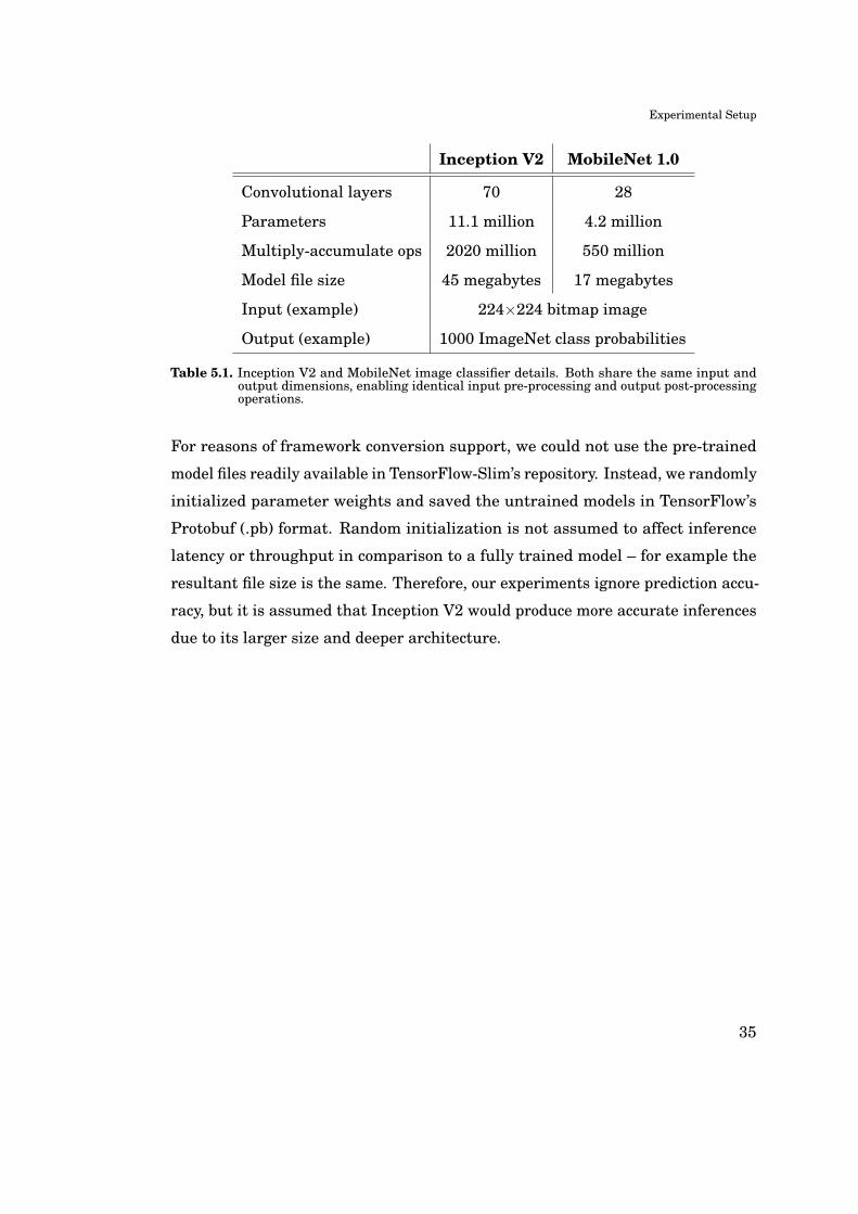
Inception V2 MobileNet 1.0

Convolutional layers 70 28

Parameters 11.1 million 4.2 million

Multiply-accumulate ops 2020 million 550 million

Model file size 45 megabytes 17 megabytes

Input (example) 224×224 bitmap image

Output (example) 1000 ImageNet class probabilities

Table 5.1. Inception V2 and MobileNet image classifier details. Both share the same input andoutput dimensions, enabling identical input pre-processing and output post-processingoperations.

For reasons of framework conversion support, we could not use the pre-trained

model files readily available in TensorFlow-Slim’s repository. Instead, we randomly

initialized parameter weights and saved the untrained models in TensorFlow’s

Protobuf (.pb) format. Random initialization is not assumed to affect inference

latency or throughput in comparison to a fully trained model – for example the

resultant file size is the same. Therefore, our experiments ignore prediction accu-

racy, but it is assumed that Inception V2 would produce more accurate inferences

due to its larger size and deeper architecture.

35

Experimental Setup

5.2 Frameworks

As briefly mentioned in Chapter 3, the two main inference frameworks in our ex-

periment are Google’s TensorFlow and Qualcomm’s Snapdragon Neural Processing

Engine. Specifically, the following API library versions are used:

• TensorFlow Mobile Java API 1.5.0-rc1 (hereafter TensorFlow or TF)

• TensorFlow Lite 0.1.1 (TF Lite)

• Qualcomm Snapdragon Neural Processing Engine 1.10.1

(Snapdragon NPE or SNPE)

The full TensorFlow Mobile can use our chosen model files directly, but for others,

conversion from Protobuf format to a special format is needed, which is not always

possible due to varying support for neural network layer operations. For example,

at the time of our experiment, converting Inception V2 to TensorFlow Lite’s

Flatbuf format is not possible, leaving only MobileNet to be used in TF Lite’s

measurements.

Snapdragon NPE ships with an SDK that has conversion tools from both Caffe

and TensorFlow to Deep Learning Container (.dlc) files. In addition to the original

model file, the converter needs input and output layer names, as well as input

dimensions – which can be tricky since TensorFlow allows variable-length batch

and input dimensions, whereas SNPE only accepts a batch size of one and fixed

input data dimensions, for example 1×224×224×3 for images (width and height

of 224 pixels, in three RGB channels).

During our experiments, SNPE SDK received multiple version updates where

improved conversion support was promised every time, but with varying actual

success. We also had difficulties with converting TensorFlow’s pre-trained example

models into DLC format, therefore we had to settle for the untrained models

36

Experimental Setup

solution described in previous section.

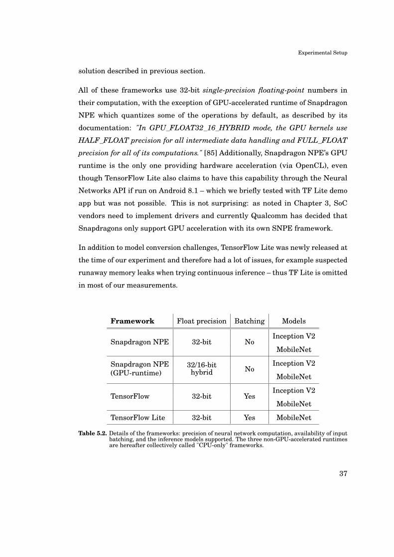
All of these frameworks use 32-bit single-precision floating-point numbers in

their computation, with the exception of GPU-accelerated runtime of Snapdragon

NPE which quantizes some of the operations by default, as described by its

documentation: "In GPU_FLOAT32_16_HYBRID mode, the GPU kernels use

HALF_FLOAT precision for all intermediate data handling and FULL_FLOAT

precision for all of its computations." [85] Additionally, Snapdragon NPE’s GPU

runtime is the only one providing hardware acceleration (via OpenCL), even

though TensorFlow Lite also claims to have this capability through the Neural

Networks API if run on Android 8.1 – which we briefly tested with TF Lite demo

app but was not possible. This is not surprising: as noted in Chapter 3, SoC

vendors need to implement drivers and currently Qualcomm has decided that

Snapdragons only support GPU acceleration with its own SNPE framework.

In addition to model conversion challenges, TensorFlow Lite was newly released at

the time of our experiment and therefore had a lot of issues, for example suspected

runaway memory leaks when trying continuous inference – thus TF Lite is omitted

in most of our measurements.

Framework Float precision Batching Models

Snapdragon NPE 32-bit NoInception V2

MobileNet

Snapdragon NPE(GPU-runtime)

32/16-bithybrid No

Inception V2

MobileNet

TensorFlow 32-bit YesInception V2

MobileNet

TensorFlow Lite 32-bit Yes MobileNet

Table 5.2. Details of the frameworks: precision of neural network computation, availability of inputbatching, and the inference models supported. The three non-GPU-accelerated runtimesare hereafter collectively called "CPU-only" frameworks.

37

Experimental Setup

5.3 Testbed Overview

The Device

Nokia 8 [90] by HMD was chosen as the testbed device for our experiment, for

several reasons. Firstly, it has one of the "cleanest" installations of the latest

version of Android OS (8.0 Oreo), meaning that there are less pre-installed apps

and background services. Secondly, Nokia 8 supports OpenCL which enables

GPU acceleration. And finally, it has a top-of-the-line Snapdragon SoC from

Qualcomm, which is required for running the Snapdragon Neural Processing

Engine framework.

Snapdragon 835 [91] has an eight-core Kryo 280 CPU in a fully HMP-capable

big.LITTLE configuration: 1.9 GHz "efficiency" cluster and 2.45 GHz "perfor-

mance" cluster. Although HMP enables using all cores simultaneously, the fre-

quency governor scales clock speeds per cluster instead of each core individually. In

other words, "efficiency" cores always have the same frequency among themselves

and "performance" cores likewise their own. We use the default frequency scaling

governor, interactive, with sampling delay parameters set by the manufacturer to

19 milliseconds instead of Android Linux kernel default 80 ms. This means that

the CPU should respond faster to load changes.

The graphics processor in Snapdragon 835 is the 710 Mhz Adreno 540, with

presumably Qualcomm’s default msm-adreno-tz as GPU frequency governor. We

were unable to confirm this since the non-CPU governor configuration files require

root access to read, but the GPU clock frequency definitely appears to scale with

the computing load.

The lithium-ion polymer battery in Nokia 8 has a typical modern smartphone

capacity of 3090 mAh with nominal voltage of 3.85V, meaning the total energy

storage is around 43 kilojoules or 11.9 watt-hours.

38

Experimental Setup

The Application

Our testbed application is a regular Android app developed with the latest Android

Studio IDE [92], with build settings targeted at the highest Android 8.0 API levels.

With the exception of the normal camera access permission, the app does not

require any special privileges or run priorities.

Snapdragon NPE library files are available as part of its SDK in Android Archive

(AAR) format, whereas TensorFlow is fetched at app build time from Google’s

Maven repository2. Both frameworks need native C/C++ code support via Android

NDK, with 64-bit ARM architecture arm64-v8a/AArch64 selected as target Appli-

cation Binary Interface3. However, the first versions of SNPE SDK we tested did

not support AArch64 which is quite peculiar for a framework that is supposed to

be run on the latest 64-bit Snapdragon SoCs. Luckily 64-bit support was added

before our final measurements.

The model files are located in the assets-folder to be included within the built

application. However, this increases the installation size of the app significantly –

which is not a problem for experimental research applications but can be an issue

in real-life production releases.

The acquisition of input images is achieved through Android’s Camera2 API4,

using the phone’s rear-facing camera pointed at floor from one meter height in

normal room lighting conditions. Camera capture settings are hard-coded as

480×640 pixel preview quality JPEG images, with the exposure time fixed to 1/60

seconds to prevent capture latency fluctuations. Other settings are left at defaults

or set to "automatic". For most measurements, the camera thread is launched

with a setRepeatingRequest to continuously capture new images for inference.

Normally the application launches into a before-run settings UI, but for most

experiments the actual measurement run is started from Android Studio with

2https://bintray.com/google/tensorflow3https://developer.android.com/ndk/guides/abis.html4https://developer.android.com/reference/android/hardware/camera2/package-summary.html

39

Experimental Setup

USB-debugging and logging on. The app also includes a debug UI for on-screen

printing of intermediate timing results and a camera preview, but it was not used

for the final measurements.

Before running the experiments, the screen is set to maximum brightness and

also kept always on with keepScreenOn UI attribute. All network communications

(WiFi and cellular) are turned off. Also no other apps are started, except for the

default system background processes, or the profiler app when making power

measurements.

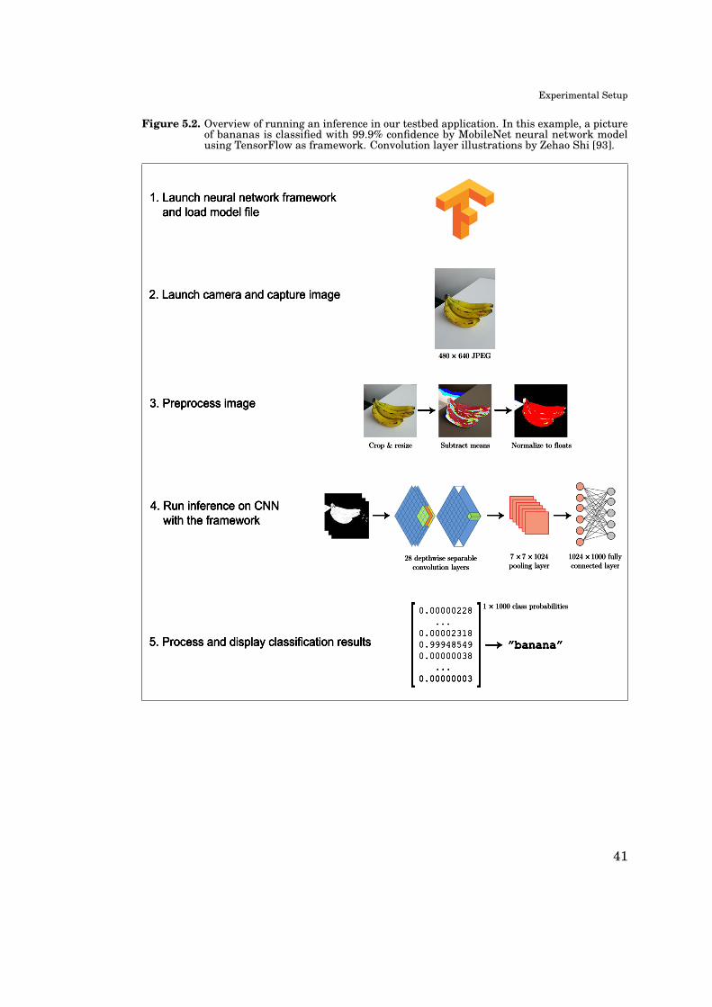
Details of the different measurement runs vary (see Table 5.3), but Figure 5.2

presents a general overview of one inference from start to finish. The process is

divided into five subtasks of which the actual CNN inference is only one part. Be-

cause our study ignores the prediction accuracy, only subtasks 1 to 4 are part of the

performance measurements, leaving out the last subtask where the classification

results would be presented to user.

Figure 5.1. Left: Nokia 8, our test phone, attached to PC with USB cable, displaying the before-runsettings UI of the app.Right: battery-powered measurement in progress, with rear camera pointed at floor.

40

Experimental Setup

Figure 5.2. Overview of running an inference in our testbed application. In this example, a pictureof bananas is classified with 99.9% confidence by MobileNet neural network modelusing TensorFlow as framework. Convolution layer illustrations by Zehao Shi [93].

480 × 640 JPEG

Crop & resize Subtract means Normalize to floats

28 depthwise separableconvolution layers

7 × 7 × 1024pooling layer

1024 × 1000 fullyconnected layer

1 × 1000 class probabilities

”banana”

0.00000228 ...0.000023180.999485490.00000038 ...0.000000030.00000003

[ ]

1. Launch neural network framework and load model file

2. Launch camera and capture image

3. Preprocess image

4. Run inference on CNN with the framework

5. Process and display classification results

41

Experimental Setup

5.4 Performance Measurements

This section presents our performance measurement methods in detail. Table 5.3

shows which frameworks are available for which measurement, sources of the

performance data points (instruments), and how the test device is powered during

the experiment.

Measurement Frameworks Instruments Power supply

Latency All Timing USB cable

Throughput All Timing USB cable

Batch size vs. throughput TF Timing USB cable

Memory usage TF, SNPE Android Profiler USB cable

CPU Temperature TF Snapdragon Profiler USB cable

Sustained throughputTiming +

Trepn ProfilerCPU/GPU frequencies TF, SNPE Battery

Power consumption

Table 5.3. Details of performance measurements.

In addition to timing functions inside application code, we use three profiling

software as instruments:

• Android Profiler [94], a tool provided with Android Studio, that can display for

example an application’s processor and memory usage.

• Trepn Power Profiler [95] developed by Qualcomm, is an on-device app suitable

for battery-powered runs.

• Snapdragon Profiler [96], also from Qualcomm, is installed on a desktop OS and

then profiles the phone through USB connection.

42

Experimental Setup

Additionally, we utilize threading in the experiment in two ways: firstly, as men-

tioned in Chapter 4, Android best practices suggest using AsyncTasks for non-UI

computation outside the main thread. In all runs of our application, individual

subtasks are processed in their own AsyncTask threads. Secondly, as an additional

performance parameter, we initialize one or two instances of the neural network

model to study concurrent inference. This is done in all experiments with the

exception of single inference latency in which deploying multiple network instances

would be pointless.

Latency measurements are calculated by logging the execution times with high-

resolution System.nanoTime timer class5. Each subtask starts its own timer and

when finished, reports the elapsed latency to the main thread for logging. In-

task timing is required also because System.nanoTime does not produce globally

synced clock values and thus cannot be used across threads. The logged latency

timings of individual runs are added into a Python script file from which the

final measurement results – average values with 95% confidence intervals – are

presented in milliseconds.

Throughput is calculated by running inference on a bulk of multiple images. The

unit of throughput, inferences per second, is calculated by dividing the number

of finished inferences (the bulk size) with the total run time. The latency of

neural network model load and camera setup, i.e. subtasks 1 and 2 in Figure

5.2, are excluded from the total run time. Similar to latency, the throughput

measurements are also averaged results from System.nanoTime logging, in this case

clocked inside the main thread: the bulk timer is started after camera and net

model have been loaded, and stopped when the final image of the bulk has been

inferenced. Therefore, different bulk sizes can be used, in our measurements

between 100 to 1000 images. The device is also powered off between bulk runs to

cool down and avoid thermal throttling of processor frequencies, with the obvious

exception of bulks within a sustained throughput measurement run.

Batch size vs. throughput is actually an intermediate measurement made5https://developer.android.com/reference/java/lang/System.html#nanoTime()

43

Experimental Setup

for TensorFlow to discover the behavior of batching, in which the batch size is

incremented to increase throughput with a penalty of higher per-batch latency.

The result from this measurement was used to find the "sweet spot" batch size

of ten images, used subsequently in all sustained inference measurements. The

batch vs. throughput behavior is described in more detail in the next chapter.

Memory usage of the test application is studied directly from output graphs of

Android Profiler, when running a bulk of 150 images on each of the test frameworks

– excluding TensorFlow Lite which could not produce reliably reproducible runs.

CPU Temperature tells the current SoC die temperature. After reaching a

certain temperature limit, DVFS throttles CPU frequencies down to cool down a

while. The CPU temperature data point is only available through Snapdragon

Profiler, which means that we cannot measure it during battery-powered runs.

Moreover, when connected to Snapdragon Profiler, only TensorFlow framework

can be used without errors. We suspect that this is because SNPE and the Profiler

might try to use the same libraries or some other system API simultaneously,

causing the app to crash.

Sustained throughput measurements run the inference continuously and long

enough to possibly cause DVFS to downscale processor frequencies due to risk of

overheating. We study the effect of this throttling on the inference throughput

over time – especially when running with the CPU-only frameworks, which we

also test under different environmental temperatures. Each framework is given

between 3000 and 9000 images to run inference on, enough to finish in between 10

to 20 minutes. The instant throughput is calculated in bulks every 150 inferences.

TensorFlow Lite is excluded from all sustained inference experiments.

In addition to throughput progression, the following metrics are logged simultane-

ously within each of the sustained throughput runs:

CPU/GPU frequencies can be recorded with either Trepn or Snapdragon Profiler,

but we mostly use Trepn. In addition to the currently set clock frequencies, some

44

Experimental Setup

profiling apps can also measure CPU and GPU utilization percentage, but in our

initial test runs we saw that the utilization data is very noisy and does not produce

as interesting results as frequency values do. Because the CPU clock speeds in

Snapdragon 835 are governed per-cluster, we measure only one core from each as

a representative for "big" and "LITTLE" to reduce the amount of data points and

thus profiling overhead. Each Trepn profiling session is started programmatically

from application code, and the data point gathering interval is set to its finest

allowed value, 100 milliseconds.

Power consumption is also recorded with Trepn Power Profiler. It can report the

current power consumption of either a specified application or the whole system.

We choose to use system-level power profiling because it is assumed to be more

accurate and based on actual device wattage, whereas determining the share of

power usage of an individual app would only be a rough estimation. Of course

this means that some of the results presented in the next chapter, for example

inferences per unit of energy, can only be used in comparison with each other,

because the inference subtask does not spend all of the power by itself.

Since we are not particularly interested in energy efficiency rather than the

characteristics of maximum performance, we do not use the features from Android

Sustained Performance API. This is also behind the decision to keep the phone

screen on at full brightness: we want to push the system’s power consumption to

its limit to potentially reveal some interesting behavior. This and much more is

covered in the next chapter, which presents our experimental results.

45

6. Experimental Results

This chapter presents the results and describes the outcomes of our experimental

measurements. The first performance figures presented are for single inference

latency, followed by continuous inference throughput charts and remarks on Ten-

sorFlow’s batching in the second section, ending with the profiling results of

application memory usage. The third section is devoted to performance in sus-

tained continuous inference: the results of these long runs reveal the progression

of throughput, changes in power consumption, CPU/GPU core frequencies, and

CPU temperature, over the course of the run.

To save space, graphs of some measurements with MobileNet model, such as

memory usage and sustained continuous runs, are not displayed because Inception

V2 results are more clear but similar enough to present the same implications.

The extra MobileNet graphs can be found in Appendix A. Also to note, Figures 6.1,

6.2, 6.3, and 6.4 are partially the same as in our previous work [15].

46

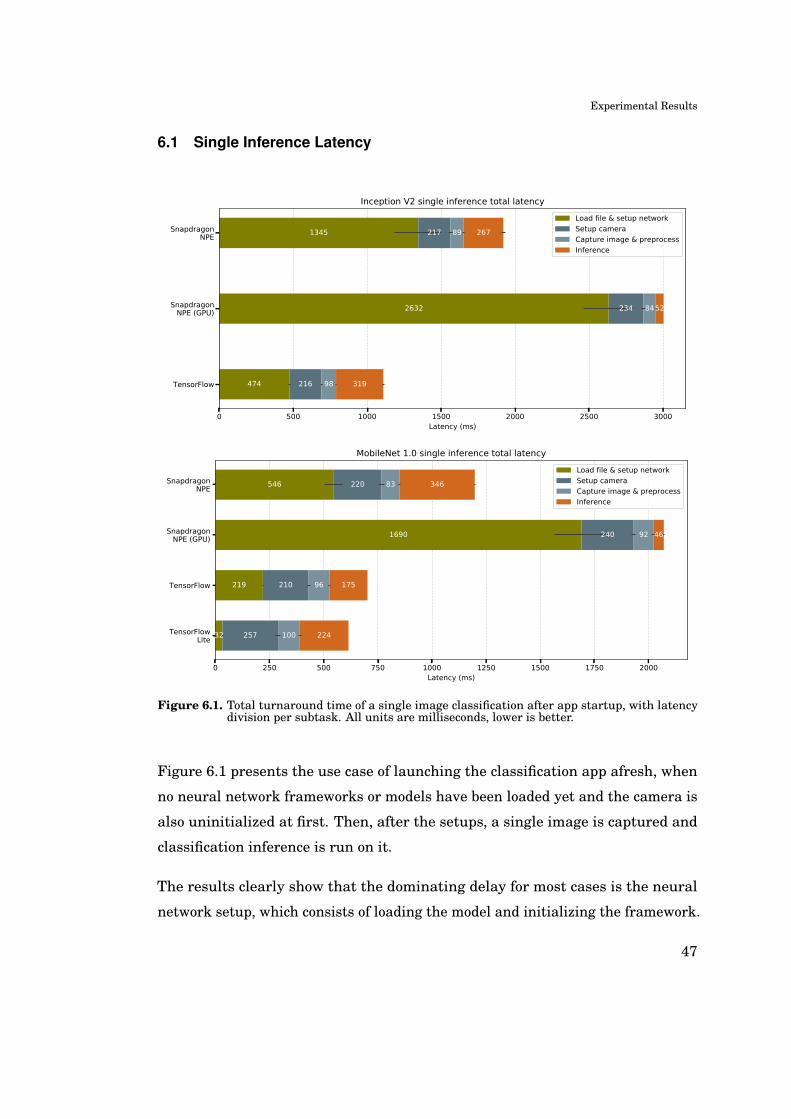
Experimental Results

6.1 Single Inference Latency

0 500 1000 1500 2000 2500 3000Latency (ms)

SnapdragonNPE

SnapdragonNPE (GPU)

TensorFlow

1345 217 89 267

2632 234 8452

474 216 98 319

Inception V2 single inference total latency

Load file & setup networkSetup cameraCapture image & preprocessInference

0 250 500 750 1000 1250 1500 1750 2000Latency (ms)

SnapdragonNPE

SnapdragonNPE (GPU)

TensorFlow

TensorFlowLite

546 220 83 346

1690 240 92 46

219 210 96 175

32 257 100 224

MobileNet 1.0 single inference total latency

Load file & setup networkSetup cameraCapture image & preprocessInference

Figure 6.1. Total turnaround time of a single image classification after app startup, with latencydivision per subtask. All units are milliseconds, lower is better.

Figure 6.1 presents the use case of launching the classification app afresh, when

no neural network frameworks or models have been loaded yet and the camera is

also uninitialized at first. Then, after the setups, a single image is captured and

classification inference is run on it.

The results clearly show that the dominating delay for most cases is the neural

network setup, which consists of loading the model and initializing the framework.

47

Experimental Results

Their latencies cannot be calculated separately since all frameworks take the

model file pointer as network initialization parameter. In some cases, camera

setup and image capture subtasks also take longer time to process than the actual

inference task. The exception is TensorFlow Lite which apparently does not

actually initialize the network until the first inference, though its total latency

with MobileNet is nevertheless the fastest at just over 600 ms.

The main takeaway is the severe turnaround latency of GPU-accelerated Snap-

dragon NPE: although the inference part itself is fast (46ms to 52ms), the network

setup latency with either model is slower than any other frameworks’ total latency,

pushing SNPE GPU’s total finishing time to between two and three seconds. The

CPU-only runtime of Snapdragon NPE does not perform that well either: it also

has a long setup time, and for unknown reason a slower inference latency with

MobileNet than with the heavier Inception V2.

In addition to TF Lite, we also noticed that the full version of TensorFlow also

leaves some parts of the network setup to be finished within the first inference,

after which subsequent images are then processed faster. This of course is not

revealed by these single inference results but becomes apparent in the continuous

throughput results in the next section.

48

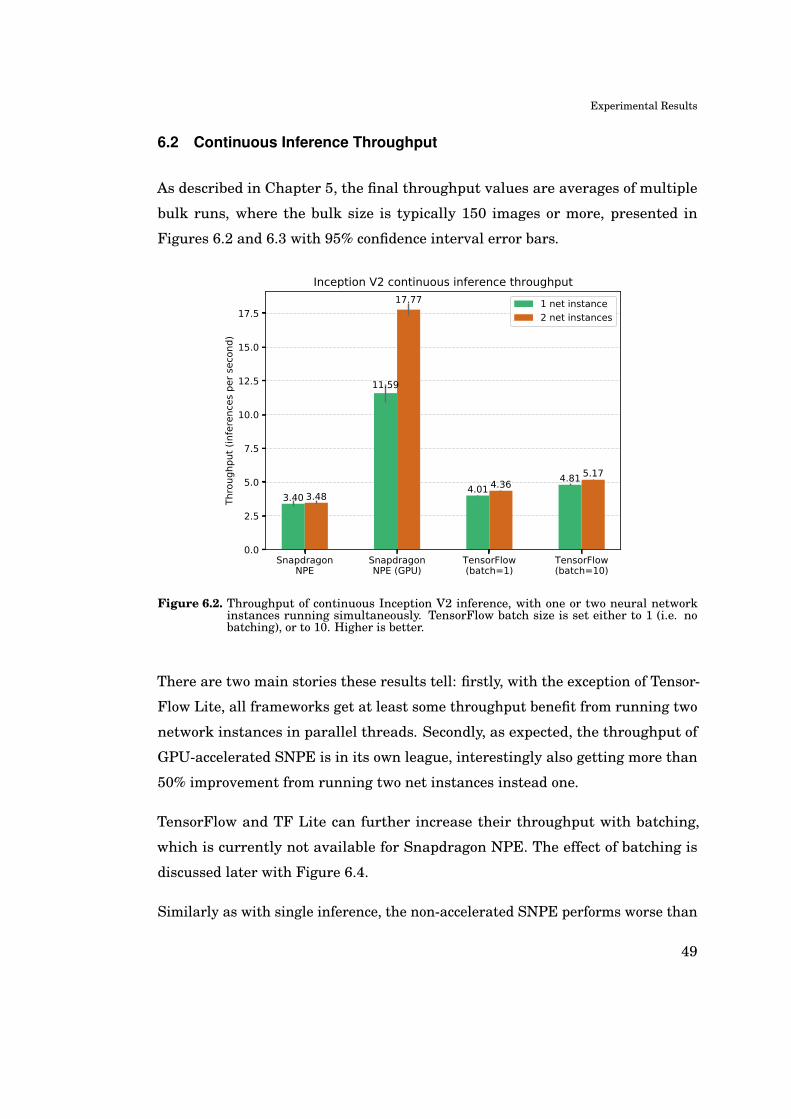
Experimental Results

6.2 Continuous Inference Throughput

As described in Chapter 5, the final throughput values are averages of multiple

bulk runs, where the bulk size is typically 150 images or more, presented in

Figures 6.2 and 6.3 with 95% confidence interval error bars.

SnapdragonNPE

SnapdragonNPE (GPU)

TensorFlow(batch=1)

TensorFlow(batch=10)

0.0

2.5

5.0

7.5

10.0

12.5

15.0

17.5

Thro

ughp

ut (i

nfer

ence

s pe

r sec

ond)

3.40

11.59

4.014.81

3.48

17.77

4.365.17

Inception V2 continuous inference throughput

1 net instance2 net instances

Figure 6.2. Throughput of continuous Inception V2 inference, with one or two neural networkinstances running simultaneously. TensorFlow batch size is set either to 1 (i.e. nobatching), or to 10. Higher is better.

There are two main stories these results tell: firstly, with the exception of Tensor-

Flow Lite, all frameworks get at least some throughput benefit from running two

network instances in parallel threads. Secondly, as expected, the throughput of

GPU-accelerated SNPE is in its own league, interestingly also getting more than

50% improvement from running two net instances instead one.

TensorFlow and TF Lite can further increase their throughput with batching,

which is currently not available for Snapdragon NPE. The effect of batching is

discussed later with Figure 6.4.

Similarly as with single inference, the non-accelerated SNPE performs worse than

49

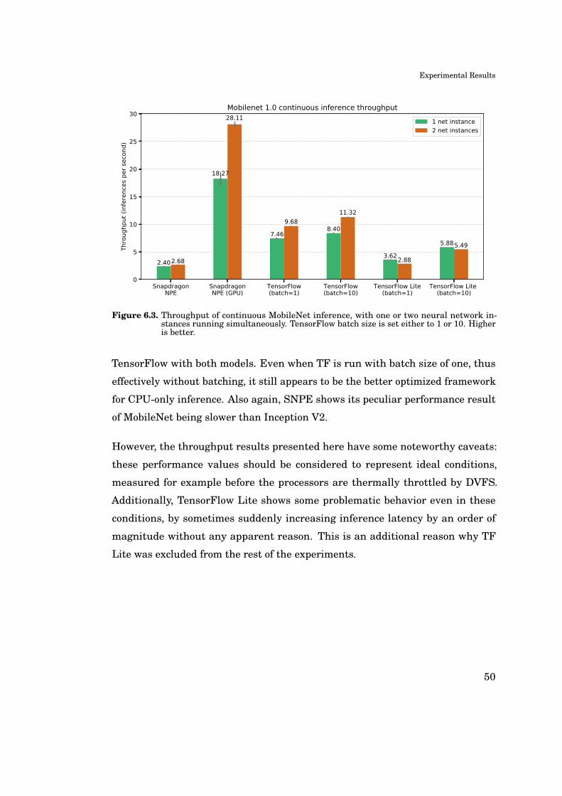
Experimental Results

SnapdragonNPE

SnapdragonNPE (GPU)

TensorFlow(batch=1)

TensorFlow(batch=10)

TensorFlow Lite(batch=1)

TensorFlow Lite (batch=10)

0

5

10

15

20

25

30Th

roug

hput

(inf

eren

ces

per s

econ

d)

2.40

18.27

7.468.40

3.62

5.88

2.68

28.11

9.6811.32

2.88

5.49

Mobilenet 1.0 continuous inference throughput

1 net instance2 net instances

Figure 6.3. Throughput of continuous MobileNet inference, with one or two neural network in-stances running simultaneously. TensorFlow batch size is set either to 1 or 10. Higheris better.

TensorFlow with both models. Even when TF is run with batch size of one, thus

effectively without batching, it still appears to be the better optimized framework

for CPU-only inference. Also again, SNPE shows its peculiar performance result

of MobileNet being slower than Inception V2.

However, the throughput results presented here have some noteworthy caveats:

these performance values should be considered to represent ideal conditions,

measured for example before the processors are thermally throttled by DVFS.

Additionally, TensorFlow Lite shows some problematic behavior even in these

conditions, by sometimes suddenly increasing inference latency by an order of

magnitude without any apparent reason. This is an additional reason why TF

Lite was excluded from the rest of the experiments.

50

Experimental Results

Batch Size: Latency vs. Throughput

Figure 6.4 describes the relationship between TensorFlow’s throughput and latency

on different batch sizes. A batch latency consists of the time it takes to preprocess

and inference a batch of N images. Throughput is calculated in the same way as

in previous measurements.

The results show that after increasing the batch size beyond five images, the

throughput improvement slows down. Therefore, as revealed in the experiment

setup chapter, we arrive at the batch size of 10 as "sweet spot" value for Ten-

sorFlow’s sustained inference measurements, results of which are presented in

Section 6.3. Additionally, having two network instances running in parallel seems

to increase the throughput without a significant latency penalty.

4.0 4.2 4.4 4.6 4.8 5.0 5.2Throughput (inferences per second)

0

1000

2000

3000

4000

5000

6000

Batc

h la

tenc

y (m

s)

123

45

6789

101112

1314

1516

1718

19 2021

2223

242526

2728

29 3031

3233

12

34

567

89

101112

1314

15

1617

18

19

20

Inception V2 with TensorFlow batch size latency vs. throughput

1 net instance2 net instances

Figure 6.4. Effect of batch size, varied from 1 to 33, on total throughput and the latency of in-ferencing a batch. One or two neural network instances are running simultaneously,both taking same number of images per batch. The error bars denote 95% confidenceintervals for throughput.

51

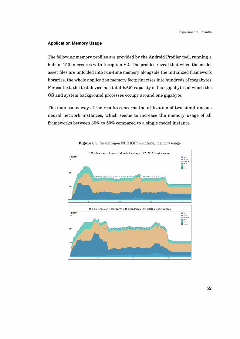
Experimental Results

Application Memory Usage

The following memory profiles are provided by the Android Profiler tool, running a

bulk of 150 inferences with Inception V2. The profiles reveal that when the model

asset files are unfolded into run-time memory alongside the initialized framework

libraries, the whole application memory footprint rises into hundreds of megabytes.

For context, the test device has total RAM capacity of four gigabytes of which the

OS and system background processes occupy around one gigabyte.

The main takeaway of the results concerns the utilization of two simultaneous

neural network instances, which seems to increase the memory usage of all

frameworks between 30% to 50% compared to a single model instance.

Figure 6.5. Snapdragon NPE (GPU-runtime) memory usage

52

Experimental Results

Figure 6.5 shows that SNPE’s GPU-accelerated runtime consumes significantly

less memory than the CPU-only frameworks. This might be because of its 32/16-bit

hybrid partial quantization of floating point numbers, which reduces the size of

the network. Also, the type of its used memory is mostly categorized as "Graphics"

which according to Android Profiler documentation means "Memory used for

graphics buffer queues to display pixels to the screen" 1. The documentation

also includes a note that the graphics memory is shared with CPU. This does

not exclude the possibility of a dedicated GPU-memory that is hidden from the

profiler graph. However, Snapdragon specifications have no mention of a dedicated

memory, which is more evidence for the memory usage really being smaller.

Figure 6.6 displays the memory usage of SNPE’s CPU-only runtime, and Figures

6.7 and 6.8 in turn TensorFlow’s with batch sizes of one or ten. Notice the large

amount of "Native" memory, which is allocated from C/C++ code presumably by

the neural network frameworks.

The tiny trashcan symbols denote automatic garbage collection events by the Java

Virtual Machine, which assumably discard input images after use. This is clearly

visible in the larger batches of TensorFlow that temporarily increase the memory

usage, and is as expected in the "spikes" of Java-allocated memory that arise from

the preprocessing of an image batch. However, the memory footprint of the input

images, even though stored in uncompressed float arrays to wait for inference, is

in the order of a few megabytes – very little compared to the memory usage of the

neural network.

1https://developer.android.com/studio/profile/memory-profiler.html

53

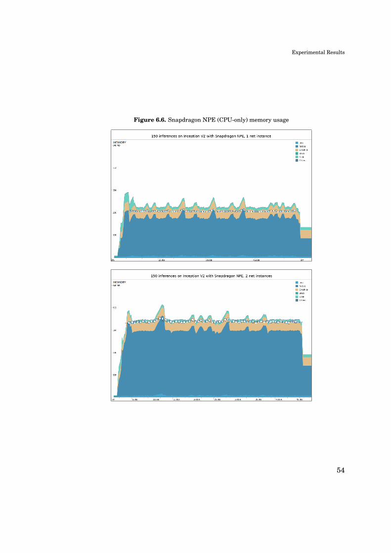
Experimental Results

Figure 6.6. Snapdragon NPE (CPU-only) memory usage

54

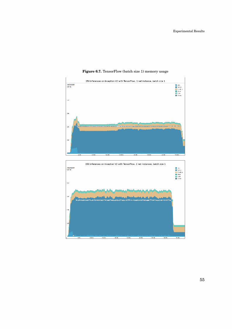
Experimental Results

Figure 6.7. TensorFlow (batch size 1) memory usage

55

Experimental Results

Figure 6.8. TensorFlow (batch size 10) memory usage

56

Experimental Results

6.3 Sustained Continuous Inference

This section focuses on the second goal of our experiment: the progression of per-

formance in continuous inference, sustained for a longer time. First, throughput

progression with Inception V2 is plotted with all of the frameworks (Figure 6.9),

then with CPU-only frameworks in different environmental temperatures (Figure

6.10), followed by power usage and processor frequency graphs from the same

runs. After that, Figure 6.14 shows changes in CPU temperature with TensorFlow,

although from a different run. And finally, Table 6.1 presents some interesting

energy and battery life calculations.

As a reminder about the setup: with the exception of CPU temperatures, all

measurements were carried out on battery power with Trepn Profiler set to its

finest profiling interval, 100ms. However, the presented graphs plot the profiling

values with a 5-second moving average. In turn, the throughput is evaluated

every 150 inferences, i.e. in intervals ranging from a few seconds up to a minute,

depending on the framework’s inference speed. The batch size of TensorFlow is

also hereafter fixed to 10.

57

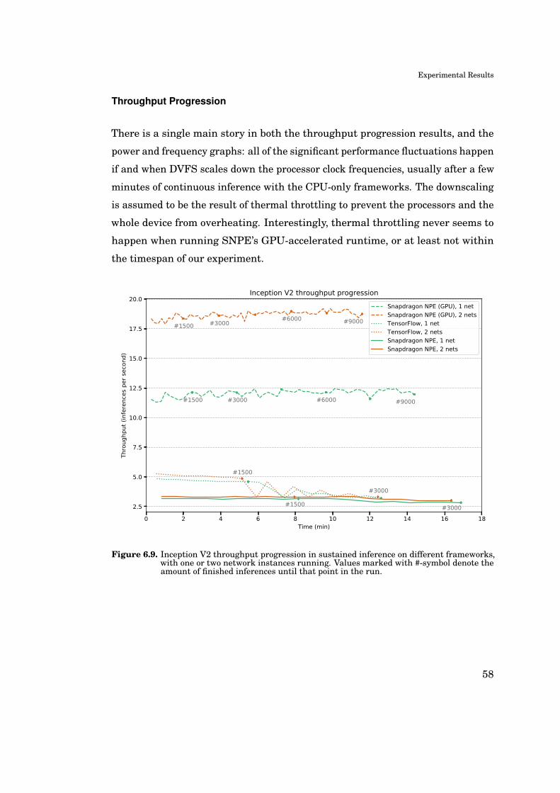
Experimental Results

Throughput Progression

There is a single main story in both the throughput progression results, and the

power and frequency graphs: all of the significant performance fluctuations happen

if and when DVFS scales down the processor clock frequencies, usually after a few

minutes of continuous inference with the CPU-only frameworks. The downscaling

is assumed to be the result of thermal throttling to prevent the processors and the

whole device from overheating. Interestingly, thermal throttling never seems to

happen when running SNPE’s GPU-accelerated runtime, or at least not within

the timespan of our experiment.

0 2 4 6 8 10 12 14 16 18Time (min)

2.5

5.0

7.5

10.0

12.5

15.0

17.5

20.0

Thro

ughp

ut (i

nfer

ence

s pe

r sec

ond)

#1500 #3000

#1500 #3000#6000 #9000

#1500 #3000 #6000 #9000

#1500

#3000

Inception V2 throughput progression

Snapdragon NPE (GPU), 1 netSnapdragon NPE (GPU), 2 netsTensorFlow, 1 netTensorFlow, 2 netsSnapdragon NPE, 1 netSnapdragon NPE, 2 nets

Figure 6.9. Inception V2 throughput progression in sustained inference on different frameworks,with one or two network instances running. Values marked with #-symbol denote theamount of finished inferences until that point in the run.

58

Experimental Results

0 2 4 6 8 10 12 14 16 18Time (min)

3.0

3.5

4.0

4.5

5.0

5.5Th

roug

hput

(inf

eren

ces

per s

econ

d)

#3000

#3000 #3000

#3000

Throughput progression and ambient temperature (Inception V2)

Snapdragon NPE, room temp.TensorFlow, room temp.Snapdragon NPE, freezingTensorFlow, freezing

Figure 6.10. Inception V2 throughput progression of the CPU-only frameworks, with one networkinstance, in different ambient temperatures: room temperature is around 20 ◦C andfreezing in range of −10 ...− 5 ◦C.

Figure 6.10 suggests that a below-zero environmental temperature is enough to

keep the CPU cool and in a sustained level of performance. However, it is possible

that the experiment did not run long enough to reveal a delayed need for thermal

throttling.

59

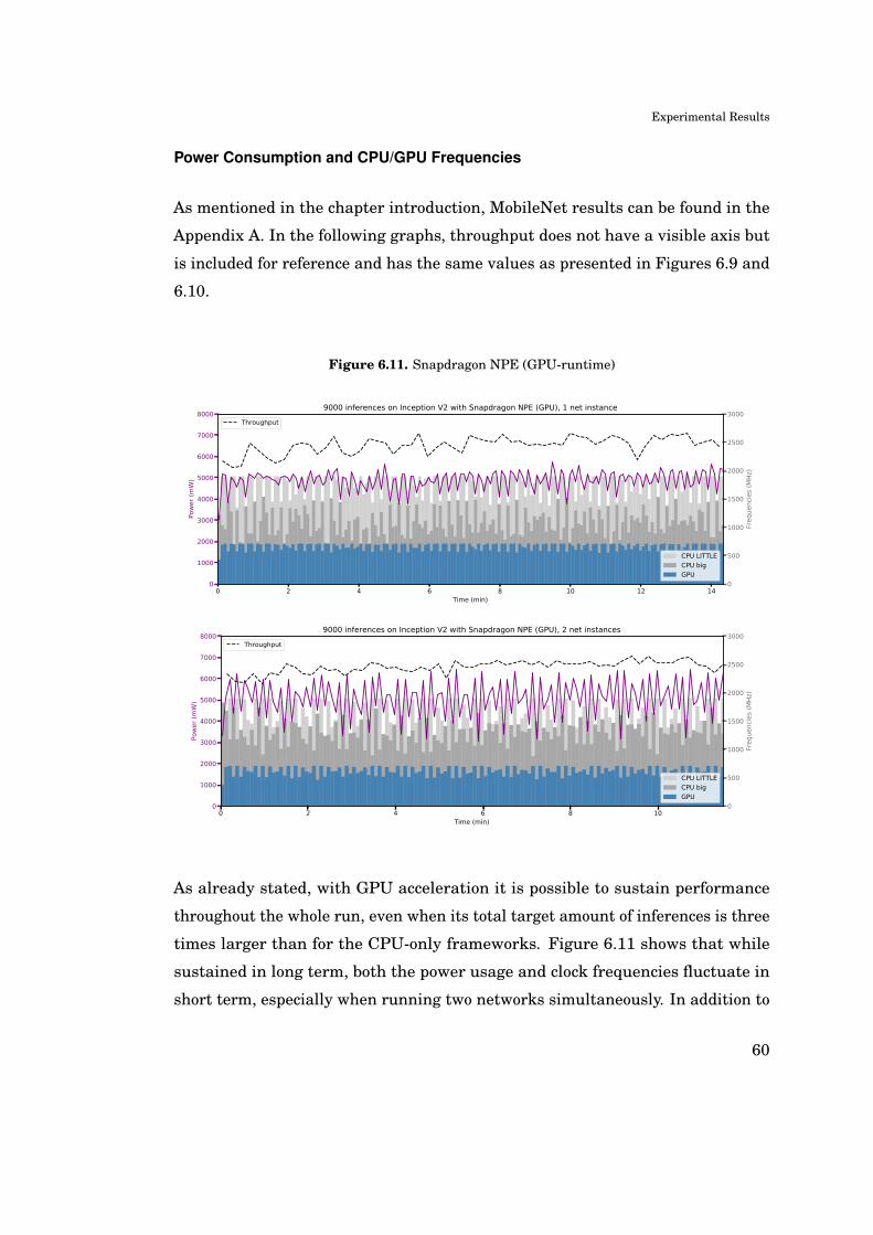
Experimental Results

Power Consumption and CPU/GPU Frequencies

As mentioned in the chapter introduction, MobileNet results can be found in the

Appendix A. In the following graphs, throughput does not have a visible axis but

is included for reference and has the same values as presented in Figures 6.9 and

6.10.

Figure 6.11. Snapdragon NPE (GPU-runtime)

0 2 4 6 8 10 12 14Time (min)

0

500

1000

1500

2000

2500

3000

Freq

uenc

ies

(MH

z)

CPU LITTLECPU bigGPU

Throughput

0

1000

2000

3000

4000

5000

6000

7000

8000

Pow

er (m

W)

9000 inferences on Inception V2 with Snapdragon NPE (GPU), 1 net instance

0 2 4 6 8 10Time (min)

0

500

1000

1500

2000

2500

3000

Freq

uenc

ies

(MH

z)

CPU LITTLECPU bigGPU

Throughput

0

1000

2000

3000

4000

5000

6000

7000

8000

Pow

er (m

W)

9000 inferences on Inception V2 with Snapdragon NPE (GPU), 2 net instances

As already stated, with GPU acceleration it is possible to sustain performance

throughout the whole run, even when its total target amount of inferences is three

times larger than for the CPU-only frameworks. Figure 6.11 shows that while

sustained in long term, both the power usage and clock frequencies fluctuate in

short term, especially when running two networks simultaneously. In addition to

60

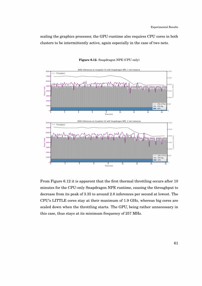
Experimental Results

scaling the graphics processor, the GPU-runtime also requires CPU cores in both

clusters to be intermittently active, again especially in the case of two nets.

Figure 6.12. Snapdragon NPE (CPU only)

0 2 4 6 8 10 12 14 16Time (min)

0

500

1000

1500

2000

2500

3000

Freq

uenc

ies

(MH

z)

CPU LITTLECPU bigGPU

Throughput

0

1000

2000

3000

4000

5000

6000

7000

8000

Pow

er (m

W)

3000 inferences on Inception V2 with Snapdragon NPE, 1 net instance

0 2 4 6 8 10 12 14 16Time (min)

0

500

1000

1500

2000

2500

3000

Freq

uenc

ies

(MH

z)

CPU LITTLECPU bigGPU

Throughput

0

1000

2000

3000

4000

5000

6000

7000

8000

Pow

er (m

W)

3000 inferences on Inception V2 with Snapdragon NPE, 2 net instances

From Figure 6.12 it is apparent that the first thermal throttling occurs after 10

minutes for the CPU-only Snapdragon NPE runtime, causing the throughput to

decrease from its peak of 3.35 to around 2.8 inferences per second at lowest. The

CPU’s LITTLE cores stay at their maximum of 1.9 GHz, whereas big cores are

scaled down when the throttling starts. The GPU, being rather unnecessary in

this case, thus stays at its minimum frequency of 257 MHz.

61

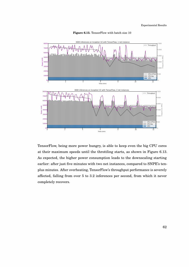
Experimental Results

Figure 6.13. TensorFlow with batch size 10

0 2 4 6 8 10 12Time (min)

0

500

1000

1500

2000

2500

3000

Freq

uenc

ies

(MH

z)

CPU LITTLECPU bigGPU

Throughput

0

1000

2000

3000

4000

5000

6000

7000

8000Po

wer

(mW

)3000 inferences on Inception V2 with TensorFlow, 1 net instance

0 2 4 6 8 10 12Time (min)

0

500

1000

1500

2000

2500

3000

Freq

uenc

ies

(MH

z)

CPU LITTLECPU bigGPU

Throughput

0

1000

2000

3000

4000

5000

6000

7000

8000

Pow

er (m

W)

3000 inferences on Inception V2 with TensorFlow, 2 net instances

TensorFlow, being more power hungry, is able to keep even the big CPU cores

at their maximum speeds until the throttling starts, as shown in Figure 6.13.

As expected, the higher power consumption leads to the downscaling starting

earlier: after just five minutes with two net instances, compared to SNPE’s ten-

plus minutes. After overheating, TensorFlow’s throughput performance is severely

affected, falling from over 5 to 3.2 inferences per second, from which it never

completely recovers.

62

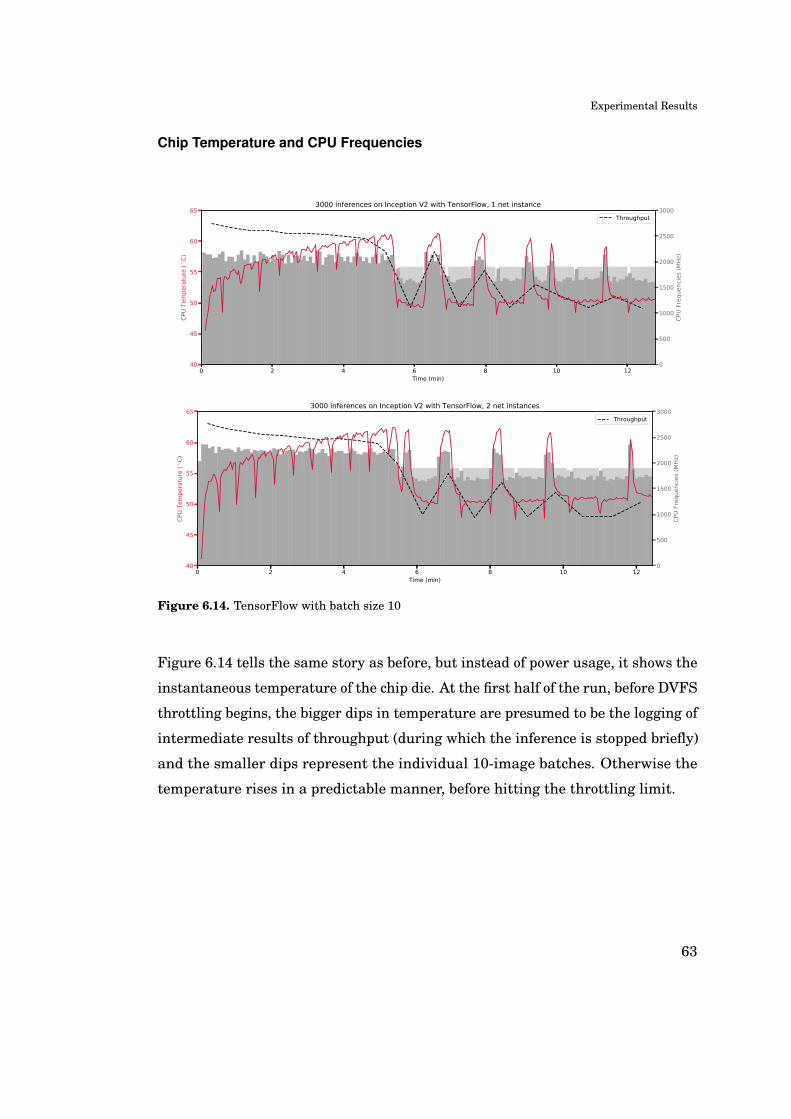
Experimental Results

Chip Temperature and CPU Frequencies

0 2 4 6 8 10 12Time (min)

0

500

1000

1500

2000

2500

3000

CPU

Fre

quen

cies

(MH

z)

Throughput

40

45

50

55

60

65

CPU

Tem

pera

ture

(C)

3000 inferences on Inception V2 with TensorFlow, 1 net instance

0 2 4 6 8 10 12Time (min)

0

500

1000

1500

2000

2500

3000

CPU

Fre

quen

cies

(MH

z)

Throughput

40

45

50

55

60

65

CPU

Tem

pera

ture

(C)

3000 inferences on Inception V2 with TensorFlow, 2 net instances

Figure 6.14. TensorFlow with batch size 10

Figure 6.14 tells the same story as before, but instead of power usage, it shows the

instantaneous temperature of the chip die. At the first half of the run, before DVFS

throttling begins, the bigger dips in temperature are presumed to be the logging of

intermediate results of throughput (during which the inference is stopped briefly)

and the smaller dips represent the individual 10-image batches. Otherwise the

temperature rises in a predictable manner, before hitting the throttling limit.

63

Experimental Results

Power and Energy

Inception V2 Power mW Inferences per mWh Battery lasts for

avg max best avg worst minutes inferences

1ne

t

SNPE (GPU) 4890 5240 8.38 7.69 7.17 146 91 400

SNPE 5190 5520 2.29 2.06 1.93 138 24 500

TensorFlow 6040 7040 3.18 2.43 2.03 118 28 200

2ne

ts

SNPE (GPU) 5090 5570 9.97 9.18 8.38 140 109 000

SNPE 5290 5600 2.37 2.09 1.97 135 24 700

TensorFlow 6030 7330 3.30 2.49 1.98 118 28 600

MobileNet Power mW Inferences per mWh Battery lasts for

avg max best avg worst minutes inferences

1ne

t

SNPE (GPU) 3990 4350 13.7 12.7 11.6 179 151 000

SNPE 4700 4860 1.99 1.66 1.59 152 19 600

TensorFlow 5630 6420 7.59 5.05 4.37 127 59 300

2ne

ts

SNPE (GPU) 4030 4660 19.8 16.6 14.4 177 198 000

SNPE 4820 4960 2.15 1.81 1.75 148 21 500

TensorFlow 6380 7310 7.79 5.67 4.84 112 66 000

Table 6.1. Power and energy consumption during sustained inference runs.The extent of battery life, assuming total capacity of 11.9 Wh, is an extrapolated estimatefrom the average power usage and run duration.

Table 6.1 presents the average and maximum power consumption of the sus-

tained inference runs, further averaged per the same 150-inference bulks as with

throughput progression in previous figures. Therefore, for example maximum

power does not represent same instant peak power than the graphs in previous

section. From these smoothed power values, an inference energy consumption

estimate can be calculated, expressed in inferences per milliwatt-hours. Although,

of course not all of the phone’s energy go to the neural network inference itself,

64

Experimental Results

but the calculation enables comparing the frameworks’ energy performance with

each other. It appears that GPU-accelerated Snapdragon NPE is again the winner,

with the best efficiency of 19.8 inferences per mWh, or 0.18 joules per inference,

when run with MobileNet and two parallel networks.

However, the "best" and "worst" energy values are theoretical and thus exaggerated

to some extent, since they can not actually be sustained for a long time. Our other

calculations from the actual average power per each of the 150-inference bulks

show that the inferences per unit of energy does not fluctuate much from the

average during the run. This means that even when throttled by DVFS, the power

usage and throughput decrease simultaneously in the same proportion.

Another interesting calculation is the estimated battery life, based on the average

wattage and the assumed battery capacity. The correctness of the estimate was

further checked by observing the actual drop in battery percentage during the

measurements, and extrapolating from that.

The results show that with our setup, TensorFlow would empty the battery in

under two hours, though providing a respectable amount of inferences in the

meantime, as compared with the CPU-only SNPE. Conversely, with an efficient

combination of GPU acceleration and MobileNet, a battery life of three hours can

be expected, while providing almost 200 thousand image classifications.

65

7. Discussion

This chapter summarizes the main outcomes of our experiment, reflects its limita-

tions, and reviews some of the challenges posed by Android and neural network

environments. The last section discusses what lies ahead for future research on

mobile neural networks.

7.1 Experimental Outcomes

Our experiments confirm the intuitive hypothesis that hardware acceleration

increases performance, namely the throughput, of neural network inference. Tra-

ditionally, increasing performance comes with a trade-off in increased resource

usage, but this appears not to be the case with mobile GPUs: offloading processing

away from the power-hungry CPU cores actually increases both computation per-

formance and energy efficiency in highly parallel tasks, such as neural network

inference.

However, GPU acceleration is only useful in continuous tasks, and basically

useless when inferencing a single image because of setup overhead. Our choice for

GPU-accelerated framework, the Snapdragon Neural Processing Engine, had an

initialization latency significantly worse than any tested frameworks’ inference

latency, for both GPU and CPU runtimes. This is remarkable because neural

network inference is usually considered to be computationally intensive, and

therefore it should intuitively be also the bottleneck of total latency.

66

Discussion

The "competitor" framework we tested against Snapdragon NPE – Google’s very

popular TensorFlow – has brilliant performance results in both single inference

latency and in CPU-optimized continuous throughput, which can be further in-

creased by choosing a suitable input batch size. On the other hand, TensorFlow

is very resource-demanding with its high power consumption and memory usage.

The Lite version of TensorFlow might address this issue but we were unable to

properly test it.

One interesting outcome is the performance boost to all frameworks given by

threading: simultaneous initialization of two instances of the same neural network

model is not only possible, but actually improves the overall inference throughput.

This might be caused by a number of reasons. Firstly, the processor clock frequency

graphs presented in Figures 6.12 and 6.13 indicate an increased utilization of

the available processors when running with two network instances – compared

to running with only one instance where there seems to be unused processing

capacity, at least with the models we used. Secondly, all the threads in our

experiment were run with default priority, thus two tasks can together get an

increased share of execution time allocated to them, out of all running processes.

Unsurprisingly however, multiple threads only increase throughput performance

with a penalty of increased memory usage. Additionally, concurrent instances of

the inference framework API need more control logic in application code and more

intelligent handling of the input and output pipelines.

Our second experiment goal was to study the changes in performance in sustained

continuous inference computation. The results produced yet another advantage

for GPU acceleration, closely related to its low power consumption: the dynamic

downscaling of processor frequency to prevent overheating was observed only

with the power-intensive CPU-only frameworks. Although with our setup, the

CPU frameworks also managed to sustain their performance when the testbed

environment conditions were changed from room temperature to freezing.

67

Discussion

7.2 Challenges with Android

As mentioned in the background literature [89], to accurately benchmark compu-

tation performance on Android is difficult due to the variable environment. One

proposed solution for stabilizing performance is to fix the processor frequency to

a constant value. Indeed, the energy efficiency oracle mentioned in Chapter 4

has an easy-to-implement opposite: the performance governor that sets the CPU

frequency permanently to maximum value. This is of course not recommended

for real-life applications: overheating is dangerous not only to the functioning of

processors, but to other smartphone hardware as well, such as batteries [97].

Another challenge in Android environment is probably the most obvious cause

for performance differences: the vast spectrum of Android devices. Hardware

differences – CPUs, GPUs, DSPs, cameras, batteries – and multiple custom

versions of the Android OS make it nearly impossible to universally compare the

performance of deep learning frameworks.

Even with the same device, software and system updates can produce changes

in measured performance: for example during our experiment, after upgrading

Android version from 7.1 Nougat to 8.0 Oreo, the camera API latencies became

slightly but clearly different than when measured with the previous Android

version. However, the changes were not significant enough to really affect the

experiment outcomes.

68

Discussion

7.3 Challenges with Neural Networks

The rapidly changing and not-quite-ready-yet environment of neural network

frameworks for mobile presented its own set of difficulties for the experiment.

Firstly, as made clear in Chapters 5 and 6, TensorFlow Lite is still unripe for

any serious production applications. Secondly, like the operating system itself,

Snapdragon NPE received multiple version updates during our experimentation,

which for example affected its network initialization latency for no documented

reason. Again, this did not change experiment outcomes but produced some rework

on the measurements.

Our initial choices for neural network architectures to study would have been

object detection models instead of classification, but we abandoned those after

several failed attempts at converting them to Snapdragon NPE’s file format. This

further confirmed the notion of poor support for any advanced neural network

layers or operations in the current deep learning frameworks.

There are multiple aspects regarding neural network models that our experiment

left unstudied. For example the insufficient processor utilization hypothesis de-

scribed in Section 7.1 could be further tested by running inference on even heavier

neural network models, such as Inception V3 [98], which could possibly give all

processor cores enough work to reach higher utilization percentages. We also

ignored any model tuning and training-related aspects, such as whether reducing

the amount of recognition classes would also improve performance. Additionally,

taking model quantization into consideration would allow experimenting with

hardware acceleration on other special-purpose processors such as DSPs, because

for example Snapdragon’s Hexagon DSP requires 8-bit integer computation.

69

Discussion

7.4 Looking Ahead

In the cutting edge world of artificial neural networks, both academic research and

industry applications are advancing simultaneously, especially since many of the

tools and frameworks are open-source. Thus, the community is quick to implement

new things, but on the other hand important work for production-readiness, such

as quality assurance, interoperability, and maintenance is often left half-done.

However, there are ongoing efforts that look promising in standardizing the neural

network world with universal frameworks, such as ONNX. Indeed, for example

right before the publication of this thesis, a newly released version of Snapdragon

NPE added experimental support for ONNX models.

On Android side, we wish good luck to the future of Neural Networks API. Addi-

tionally, we also wish for better deep learning framework tools for mobile, such

as the input pipeline performance modules already found in desktop version of

TensorFlow [99].

On mobile hardware side, there are interesting developments in processing unit

choices for neural networks computation, for example this statement about the

signal processor in the newest flagship Snapdragon: "Qualcomm claims that AI

performance with the new Hexagon 685 DSP is three times better than that of

the Snapdragon 835, though it’s unclear at the moment how that translates to

real-world usage." [100]

70

8. Conclusions

This thesis set out to study the field of mobile neural networks, especially the

possibilities for improving inference performance, mainly by GPU-based hard-

ware acceleration. The answers are clear: if supported by the chosen hardware

and software frameworks, GPU acceleration provides both significantly improved

performance and more energy efficient execution – but only in continuous applica-

tions.

Of course, the experiments presented in this thesis are limited in scope. Therefore

the extent of the answers also needs to be considered limited to the special case that

was studied: neural network image classification on an Android smartphone using

only two different models of neural network architecture. This leaves all other

kinds of neural network applications and different mobile devices unconsidered.

To conclude, in author’s personal opinion, the most heated phase of the current

artificial neural network revolution has probably passed. Especially image classi-

fication is already facing diminishing returns. From now on however, it is time

for both fine-tuned optimization and widespread adoption of deep learning appli-

cations, also in other "mobile" platforms than phones, such as autonomous cars.

After this, neural networks will no longer be called Artificial Intelligence as they

are currently marketed – just one everyday automation solution among others.

71

References

[1] Ian Goodfellow, Yoshua Bengio, and Aaron Courville. Deep Learning. MIT Press,2016. http://www.deeplearningbook.org.

[2] Yann LeCun, Yoshua Bengio, and Geoffrey E. Hinton. Deep learning. Nature,521(7553):436–444, 2015.

[3] High Scalability Blog. Jeff Dean On Large-Scale Deep Learn-ing At Google, 2016. http://highscalability.com/blog/2016/3/16/

jeff-dean-on-large-scale-deep-learning-at-google.html. Accessed 2018-03-19.

[4] Rajat Raina, Anand Madhavan, and Andrew Y. Ng. Large-scale deep unsupervisedlearning using graphics processors. In Proceedings of the 26th Annual InternationalConference on Machine Learning (ICML 2009), pages 873–880, 2009.

[5] Jeffrey Dean, Greg Corrado, Rajat Monga, Kai Chen, Matthieu Devin, Quoc V. Le,Mark Z. Mao, Marc’Aurelio Ranzato, Andrew W. Senior, Paul A. Tucker, Ke Yang,and Andrew Y. Ng. Large Scale Distributed Deep Networks. In Advances in NeuralInformation Processing Systems 25: 26th Annual Conference on Neural InformationProcessing Systems (NIPS 2012), pages 1232–1240, 2012.

[6] Stanford University. CS231n: Convolutional Neural Networks for Visual Recogni-tion, 2017. http://cs231n.github.io/convolutional-networks. Accessed 2018-03-07.

[7] Petar Velickovic. Deep learning for complete beginners: convolutional neuralnetworks with keras, Cambridge Spark, 2017. https://cambridgespark.com/content/

tutorials/convolutional-neural-networks-with-keras/index.html. Accessed 2018-02-22.

[8] Andrew G. Howard, Menglong Zhu, Bo Chen, Dmitry Kalenichenko, Weijun Wang,Tobias Weyand, Marco Andreetto, and Hartwig Adam. MobileNets: EfficientConvolutional Neural Networks for Mobile Vision Applications. arXiv preprint,arXiv:1704.04861, 2017.

72

References

[9] Benjamin F. Duffy and Daniel R. Flynn. A Year in Computer Vision. The M Tank,2017. http://www.themtank.org/a-year-in-computer-vision. Accessed 2018-02-28.

[10] Yann LeCun, Bernhard E. Boser, John S. Denker, Donnie Henderson, Richard E.Howard, Wayne E. Hubbard, and Lawrence D. Jackel. Handwritten Digit Recog-nition with a Back-Propagation Network. In Advances in Neural InformationProcessing Systems 2 (NIPS 1989), pages 396–404. Morgan Kaufmann, 1989.

[11] Y. Lecun, L. Bottou, Y. Bengio, and P. Haffner. Gradient-based learning applied todocument recognition. Proceedings of the IEEE, 86(11):2278–2324, 1998.

[12] Olga Russakovsky, Jia Deng, Hao Su, Jonathan Krause, Sanjeev Satheesh, SeanMa, Zhiheng Huang, Andrej Karpathy, Aditya Khosla, Michael Bernstein, Alexan-der C. Berg, and Li Fei-Fei. ImageNet Large Scale Visual Recognition Chal-lenge. International Journal of Computer Vision (IJCV), 115(3):211–252, 2015.http://www.image-net.org/challenges/LSVR/.

[13] Alex Krizhevsky, Ilya Sutskever, and Geoffrey E. Hinton. ImageNet Classificationwith Deep Convolutional Neural Networks. In Advances in Neural InformationProcessing Systems 25: 26th Annual Conference on Neural Information ProcessingSystems (NIPS 2012), pages 1106–1114, 2012.

[14] Jonathan Huang, Vivek Rathod, Chen Sun, Menglong Zhu, Anoop Korattikara,Alireza Fathi, Ian Fischer, Zbigniew Wojna, Yang Song, Sergio Guadarrama, andKevin Murphy. Speed/accuracy trade-offs for modern convolutional object detectors.arXiv preprint, arXiv:1611.10012, 2016.

[15] Jussi Hanhirova, Teemu Kämäräinen, Sipi Seppälä, Matti Siekkinen, VesaHirvisalo, and Antti Ylä-Jääski. Latency and Throughput Characterization ofConvolutional Neural Networks for Mobile Computer Vision. arXiv preprint,arXiv:1803.09492, 2018. Accepted to ACM Multimedia Systems Conference (MMSys2018).

[16] Jason Brownlee. What is the Difference Between Test and Validation Datasets?,2017. https://machinelearningmastery.com/difference-test-validation-datasets. Ac-cessed 2018-03-08.

[17] Dave Gershgorn. The data that transformed AI research —and possibly the world. Quartz, 2017. https://qz.com/1034972/

the-data-that-changed-the-direction-of-ai-research-and-possibly-the-world. Ac-cessed 2018-03-08.

[18] Jie Hu, Li Shen, and Gang Sun. Squeeze-and-Excitation Networks. arXiv preprint,arXiv:1709.01507, 2017.

73

References

[19] Samuel F. Dodge and Lina J. Karam. A Study and Comparison of Human and DeepLearning Recognition Performance under Visual Distortions. In 26th InternationalConference on Computer Communication and Networks (ICCCN 2017), pages 1–7.IEEE, 2017.

[20] Polytechnic University of Catalonia TelecomBCN. Memory usage and computa-tional considerations, Deep Learning for Computer Vision seminar, 2016. http:

//imatge-upc.github.io/telecombcn-2016-dlcv/slides/D2L1-memory.pdf. Accessed 2018-03-19.

[21] Sergey Ioffe and Christian Szegedy. Batch Normalization: Accelerating DeepNetwork Training by Reducing Internal Covariate Shift. arXiv preprint,arXiv:1502.03167, 2015.

[22] François Chollet. Xception: Deep Learning with Depthwise Separable Convolutions.arXiv preprint, arXiv:1610.02357, 2016.

[23] Seungyeop Han, Haichen Shen, Matthai Philipose, Sharad Agarwal, Alec Wolman,and Arvind Krishnamurthy. MCDNN: An Approximation-Based Execution Frame-work for Deep Stream Processing Under Resource Constraints. In Proceedings ofthe 14th Annual International Conference on Mobile Systems, Applications, andServices (MobiSys 2016), pages 123–136. ACM, 2016.

[24] Angshuman Parashar, Minsoo Rhu, Anurag Mukkara, Antonio Puglielli, Rang-harajan Venkatesan, Brucek Khailany, Joel S. Emer, Stephen W. Keckler, andWilliam J. Dally. SCNN: An Accelerator for Compressed-sparse ConvolutionalNeural Networks. arXiv preprint, arXiv:1708.04485, 2017.

[25] Song Han, Huizi Mao, and William J. Dally. Deep Compression: Compressing DeepNeural Network with Pruning, Trained Quantization and Huffman Coding. arXivpreprint, arXiv:1510.00149, 2015.

[26] Sourav Bhattacharya and Nicholas D. Lane. Sparsification and Separation of DeepLearning Layers for Constrained Resource Inference on Wearables. In Proceedingsof the 14th ACM Conference on Embedded Network Sensor Systems (SenSys 2016),pages 176–189, 2016.

[27] Wenlin Chen, James T. Wilson, Stephen Tyree, Kilian Q. Weinberger, and YixinChen. Compressing Neural Networks with the Hashing Trick. In Proceedings ofthe 32nd International Conference on Machine Learning (ICML 2015), volume 37 ofJMLR Workshop and Conference Proceedings, pages 2285–2294. JMLR.org, 2015.

[28] Max Jaderberg, Andrea Vedaldi, and Andrew Zisserman. Speeding up ConvolutionalNeural Networks with Low Rank Expansions. arXiv preprint, arXiv:1405.3866,2014.

74

References

[29] Benoit Jacob, Skirmantas Kligys, Bo Chen, Menglong Zhu, Matthew Tang, An-drew G. Howard, Hartwig Adam, and Dmitry Kalenichenko. Quantization andTraining of Neural Networks for Efficient Integer-Arithmetic-Only Inference. arXivpreprint, arXiv:1712.05877, December 2017.

[30] Surat Teerapittayanon, Bradley McDanel, and H. T. Kung. Distributed Deep NeuralNetworks Over the Cloud, the Edge and End Devices. In 37th IEEE InternationalConference on Distributed Computing Systems (ICDCS 2017), pages 328–339. IEEEComputer Society, 2017.

[31] Huynh Nguyen Loc, Youngki Lee, and Rajesh Krishna Balan. DeepMon: Mo-bile GPU-based Deep Learning Framework for Continuous Vision Applications.In Proceedings of the 15th Annual International Conference on Mobile Systems,Applications, and Services (MobiSys’17), pages 82–95. ACM, 2017.

[32] Google Research Blog. The neural networks behind Google Voice transcription, 2015.https://research.googleblog.com/2015/08/the-neural-networks-behind-google-voice.

html. Accessed 2018-03-09.

[33] Google Research Blog. How Google Translate squeezes deep learning onto a phone,2015. https://research.googleblog.com/2015/07/how-google-translate-squeezes-deep.

html. Accessed 2018-03-09.

[34] Xiao Zeng, Kai Cao, and Mi Zhang. MobileDeepPill: A Small-Footprint Mobile DeepLearning System for Recognizing Unconstrained Pill Images. In Proceedings ofthe 15th Annual International Conference on Mobile Systems, Applications, andServices (MobiSys’17), pages 56–67. ACM, 2017.

[35] Shuochao Yao, Shaohan Hu, Yiran Zhao, Aston Zhang, and Tarek F. Abdelzaher.DeepSense: A Unified Deep Learning Framework for Time-Series Mobile SensingData Processing. In Proceedings of the 26th International Conference on World WideWeb (WWW 2017), pages 351–360. ACM, 2017.

[36] Indra den Bakker. Battle of the Deep Learning frameworks — Part I: 2017, evenmore frameworks and interfaces, Towards Data Science (blog), 2017. https://

towardsdatascience.com/battle-of-the-deep-learning-frameworks-part-i-cff0e3841750.Accessed 2018-03-12.

[37] Sharan Chetlur, Cliff Woolley, Philippe Vandermersch, Jonathan Cohen, JohnTran, Bryan Catanzaro, and Evan Shelhamer. cuDNN: Efficient Primitives for DeepLearning. arXiv preprint, arXiv:1410.0759, 2014. https://developer.nvidia.com/cudnn.

[38] The Khronos Group. OpenCL – The open standard for parallel programming ofheterogeneous systems. https://www.khronos.org/opencl. Accessed 2018-03-13.

75

References

[39] Hugh Perkins. Coriander-dnn provides a partial implementation of the NVIDIACUDA cuDNN API, for Coriander, OpenCL 1.2, GitHub repository. https://github.

com/hughperkins/coriander-dnn. Accessed 2018-03-13.

[40] Martín Abadi, Ashish Agarwal, Paul Barham, Eugene Brevdo, Zhifeng Chen, CraigCitro, Gregory S. Corrado, Andy Davis, Jeffrey Dean, Matthieu Devin, Sanjay Ghe-mawat, Ian J. Goodfellow, Andrew Harp, Geoffrey Irving, Michael Isard, YangqingJia, Rafal Józefowicz, Lukasz Kaiser, Manjunath Kudlur, Josh Levenberg, DanMané, Rajat Monga, Sherry Moore, Derek Gordon Murray, Chris Olah, Mike Schus-ter, Jonathon Shlens, Benoit Steiner, Ilya Sutskever, Kunal Talwar, Paul A. Tucker,Vincent Vanhoucke, Vijay Vasudevan, Fernanda B. Viégas, Oriol Vinyals, PeteWarden, Martin Wattenberg, Martin Wicke, Yuan Yu, and Xiaoqiang Zheng. Tensor-Flow: Large-Scale Machine Learning on Heterogeneous Distributed Systems. arXivpreprint, arXiv:1603.04467, 2016. https://www.tensorflow.org/.

[41] Hugh Perkins. OpenCL 1.2 implementation for Tensorflow, GitHub repository.https://github.com/hughperkins/tf-coriander. Accessed 2018-03-12.

[42] Benoit Steiner. OpenCL support for TensorFlow, GitHub repository. https://github.

com/benoitsteiner/tensorflow-opencl. Accessed 2018-03-12.

[43] Keras: The Python Deep Learning library. https://keras.io. Accessed 2018-03-12.

[44] Berkeley Artificial Intelligence Research Lab. Caffe Deep Learning Framework.http://caffe.berkeleyvision.org. Accessed 2018-03-09.

[45] Berkeley Vision and Learning Center. OpenCL Caffe, GitHub repository. https:

//github.com/BVLC/caffe/tree/opencl. Accessed 2018-03-13.

[46] Facebook. Caffe2: A New Lightweight, Modular, and Scalable Deep LearningFramework. https://caffe2.ai. Accessed 2018-03-09.

[47] Integrating Caffe2 on iOS/Android. https://caffe2.ai/docs/mobile-integration.html.Accessed 2018-03-09.

[48] Apache. MXNet: A Scalable Deep Learning Framework. http://mxnet.incubator.

apache.org. Accessed 2018-03-09.

[49] Microsoft Cognitive Toolkit. https://www.microsoft.com/en-us/cognitive-toolkit. Ac-cessed 2018-03-12.

[50] AWS News Blog. Introducing Gluon: a new library for machinelearning from AWS and Microsoft. https://aws.amazon.com/blogs/aws/

introducing-gluon-a-new-library-for-machine-learning-from-aws-and-microsoft. Ac-cessed 2018-03-13.

[51] PyTorch. http://pytorch.org. Accessed 2018-03-13.

76

References

[52] AWS Facebook, Microsoft. ONNX: Open Neural Network Exchange Format. https:

//onnx.ai. Accessed 2018-03-09.

[53] Google. TensorFlow Mobile. https://www.tensorflow.org/mobile. Accessed 2018-03-15.

[54] Google. Introduction to TensorFlow Lite. https://www.tensorflow.org/mobile/tflite.Accessed 2018-03-07.

[55] Google. Neural Networks API. Android Developers. https://developer.android.com/

ndk/guides/neuralnetworks/index.html. Accessed 2018-03-07.

[56] Qualcomm. Snapdragon Neural Processing Engine SDK for AI. https://developer.

qualcomm.com/software/snapdragon-neural-processing-engine. Accessed 2018-02-28.

[57] Apple. Core ML. https://developer.apple.com/documentation/coreml. Accessed 2018-03-09.

[58] Apple. Metal Performance Shaders. https://developer.apple.com/documentation/

metalperformanceshaders. Accessed 2018-03-12.

[59] Chen Zhang, Peng Li, Guangyu Sun, Yijin Guan, Bingjun Xiao, and Jason Cong.Optimizing FPGA-based Accelerator Design for Deep Convolutional Neural Net-works. In Proceedings of the 2015 ACM/SIGDA International Symposium onField-Programmable Gate Arrays, pages 161–170. ACM, 2015.

[60] Tianshi Chen, Zidong Du, Ninghui Sun, Jia Wang, Chengyong Wu, Yunji Chen,and Olivier Temam. DianNao: a small-footprint high-throughput accelerator forubiquitous machine-learning. In Architectural Support for Programming Languagesand Operating Systems (ASPLOS ’14), pages 269–284. ACM, 2014.

[61] Google. Cloud TPUs - ML accelerators for TensorFlow. https://cloud.google.com/tpu.Accessed 2018-03-19.

[62] Akhil Mathur, Nicholas D. Lane, Sourav Bhattacharya, Aidan Boran, ClaudioForlivesi, and Fahim Kawsar. DeepEye: Resource Efficient Local Execution ofMultiple Deep Vision Models using Wearable Commodity Hardware. In Proceedingsof the 15th Annual International Conference on Mobile Systems, Applications, andServices (MobiSys’17), pages 68–81. ACM, 2017.

[63] Mohammad Motamedi, Daniel Fong, and Soheil Ghiasi. Cappuccino: Effi-cient Inference Software Synthesis for Mobile System-on-Chips. arXiv preprint,arXiv:1707.02647, 2017. GitHub repository: https://github.com/mtmd/Mobile_ConvNet.Accessed 2018-03-15.

[64] NVIDIA. Tegra Mobile Processors. http://www.nvidia.com/object/tegra.html. Accessed2018-03-09.

77

References

[65] Cross-compile Android demo for CUDA / State of GPU support for commercial An-droid devices, GitHub issues, 2016-2017. https://github.com/tensorflow/tensorflow/

issues/663, https://github.com/tensorflow/tensorflow/issues/11300. Accessed 2018-03-15.

[66] Linh Nguyen, Peifeng Yu, and Mosharaf Chowdhury. No!: Not Another Deep Learn-ing Framework. In Proceedings of the 16th Workshop on Hot Topics in OperatingSystems (HotOS 2017), pages 88–93, 2017.

[67] PyTorch. Transfering a model from PyTorch to Caffe2 and Mobile using ONNX. http://pytorch.org/tutorials/advanced/super_resolution_with_caffe2.html. Accessed 2018-03-09.

[68] Matthew Halpern, Yuhao Zhu, and Vijay Janapa Reddi. Mobile CPU’s rise to power:Quantifying the impact of generational mobile CPU design trends on performance,energy, and user satisfaction. In 2016 IEEE International Symposium on HighPerformance Computer Architecture (HPCA 2016), pages 64–76. IEEE ComputerSociety, 2016.

[69] Mohammad Ashraful Hoque, Matti Siekkinen, Jonghoe Koo, and Sasu Tarkoma.Full Charge Capacity and Charging Diagnosis of Smartphone Batteries. IEEETrans. Mob. Comput., 16(11):3042–3055, 2017.

[70] Aaron Carroll and Gernot Heiser. An Analysis of Power Consumption in a Smart-phone. In 2010 USENIX Annual Technical Conference. USENIX Association, 2010.

[71] Etienne Le Sueur and Gernot Heiser. Dynamic voltage and frequency scaling: Thelaws of diminishing returns. In Proceedings of the 2010 international conference onPower aware computing and systems, pages 1–8. USENIX Association, 2010.

[72] Volker Seeker. User Experience Driven CPU Frequency Scaling On Mobile DevicesTowards Better Energy Efficiency. PhD thesis, School of Informatics, University ofEdinburgh, 2017. http://www.volkerseeker.com/files/papers/2017_thesis.pdf.

[73] Dominik Brodowski. CPUFreq – User Guide. Linux Kernel Documentation. https:

//www.kernel.org/doc/Documentation/cpu-freq/user-guide.txt. Accessed 2018-03-20.

[74] Linux CPUFreq – Governors. Android Open Source Project Documentation.https://android.googlesource.com/kernel/msm/+/android-8.0.0_r0.30/Documentation/

cpu-freq/governors.txt. Accessed 2018-03-19.

[75] Arm Developer. Technologies – big.LITTLE. https://developer.arm.com/technologies/

big-little. Accessed 2018-03-19.

[76] Brian Jeff. big.LITTLE technology moves towards fully heterogeneous globaltask scheduling. ARM White Paper, 2013. https://www.arm.com/files/pdf/big_LITTLE_

technology_moves_towards_fully_heterogeneous_Global_Task_Scheduling.pdf.

78

References

[77] Nicholas D. Lane, Sourav Bhattacharya, Petko Georgiev, Claudio Forlivesi, Lei Jiao,Lorena Qendro, and Fahim Kawsar. DeepX: A Software Accelerator for Low-PowerDeep Learning Inference on Mobile Devices. In 15th ACM/IEEE InternationalConference on Information Processing in Sensor Networks (IPSN 2016), pages 23:1–23:12. IEEE, 2016.

[78] Kwang-Ting Cheng and Yi-Chu Wang. Using mobile GPU for general-purposecomputing–a case study of face recognition on smartphones. In InternationalSymposium on VLSI Design, Automation and Test (VLSI-DAT 2011), pages 1–4.IEEE, 2011.

[79] Android Modders Guide. CPU Governors, Hotplug drivers and GPU governors,2017. https://androidmodguide.blogspot.com/p/blog-page.html. Accessed 2018-03-19.

[80] Peng Du, Rick Weber, Piotr Luszczek, Stanimire Tomov, Gregory D. Peterson, andJack J. Dongarra. From CUDA to OpenCL: Towards a performance-portable solutionfor multi-platform GPU programming. Parallel Computing, 38(8):391–407, 2012.

[81] Google. RenderScript Overview. Android Developers. https://developer.android.com/

guide/topics/renderscript/compute.html. Accessed 2018-03-12.

[82] Seyyed Salar Latifi Oskouei, Hossein Golestani, Matin Hashemi, and Soheil Ghiasi.CNNdroid: GPU-Accelerated Execution of Trained Deep Convolutional NeuralNetworks on Android. In Proceedings of the 2016 ACM Conference on MultimediaConference (MM 2016), pages 1201–1205. ACM, 2016. GitHub repository: https:

//github.com/ENCP/CNNdroid. Accessed 2018-03-15.

[83] UCLA Networked & Embedded Systems Laboratory. RSTensorFlow – Ren-derScript Supported TensorFlow Ops, GitHub repository. https://github.com/

nesl/RSTensorFlow/tree/matmul_and_conv/tensorflow/contrib/android_renderscript_ops.Accessed 2018-03-15.

[84] Nicholas D. Lane, Petko Georgiev, and Lorena Qendro. DeepEar: robust smartphoneaudio sensing in unconstrained acoustic environments using deep learning. InProceedings of the 2015 ACM International Joint Conference on Pervasive andUbiquitous Computing (UbiComp 2015), pages 283–294. ACM, 2015.

[85] Qualcomm. Snapdragon Neural Processing Engine SDK - Reference Guide. https:

//developer.qualcomm.com/software/snapdragon-neural-processing-engine-ai/tools. Ac-cessed 2018-02-28.

[86] PJ Jacobowitz. TensorFlow machine learning now optimizedfor the Snapdragon 835 and Hexagon 682 DSP. QualcommOnQ blog, 2017. https://www.qualcomm.com/news/onq/2017/01/09/

tensorflow-machine-learning-now-optimized-snapdragon-835-and-hexagon-682-dsp.Accessed 2018-03-20.

79

References

[87] Google. Threading Performance. Android Developers. https://developer.android.com/topic/performance/threads.html. Accessed 2018-03-21.

[88] Mohammad Motamedi, Daniel Fong, and Soheil Ghiasi. Machine Intelligence onResource-Constrained IoT Devices: The Case of Thread Granularity Optimizationfor CNN Inference. ACM Trans. Embedded Comput. Syst., 16(5):151:1–151:19, 2017.

[89] Yao Guo, Yunnan Xu, and Xiangqun Chen. Freeze it if you can: Challenges andfuture directions in benchmarking smartphone performance. In Proceedings ofthe 18th International Workshop on Mobile Computing Systems and Applications(HotMobile 2017), pages 25–30. ACM, 2017.

[90] HMD Global. Nokia 8. https://www.nokia.com/en_int/phones/nokia-8. Accessed 2018-03-19.

[91] Qualcomm. Snapdragon 835 Mobile Platform. https://www.qualcomm.com/products/

snapdragon/processors/835. Accessed 2018-03-05.

[92] Google. Android Studio 3.0 – The Official IDE for Android. https://developer.android.com/studio.

[93] Zehao Shi. MobileNet build with Tensorflow, GitHub repository. https://github.com/

Zehaos/MobileNet. Accessed 2018-03-12.

[94] Google. Android Profiler in Android Studio. https://developer.android.com/studio/

preview/features/android-profiler.html. Accessed 2018-03-09.

[95] Qualcomm. Trepn Power Profiler. https://developer.qualcomm.com/software/

trepn-power-profiler. Accessed 2018-03-09.

[96] Qualcomm. Snapdragon Profiler. https://developer.qualcomm.com/software/

snapdragon-profiler. Accessed 2018-03-09.

[97] Noam Kedem. Six things to know about smartphone batteries. https://www.cnet.

com/news/six-things-to-know-about-smartphone-batteries. Accessed 2018-04-03.

[98] Christian Szegedy, Vincent Vanhoucke, Sergey Ioffe, Jonathon Shlens, and ZbigniewWojna. Rethinking the Inception Architecture for Computer Vision. arXiv preprint,arXiv:1512.00567, 2015.

[99] Google. TensorFlow Performance Guide. https://www.tensorflow.org/performance/

performance_guide. Accessed 2018-04-03.

[100] Daniel Bader. Qualcomm Snapdragon 845: Everything you need to know. An-droid Central, 2018. https://www.androidcentral.com/qualcomm-snapdragon-845. Ac-cessed 2018-04-03.

80

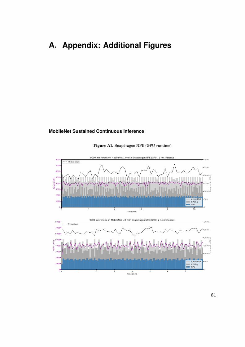
A. Appendix: Additional Figures

MobileNet Sustained Continuous Inference

Figure A1. Snapdragon NPE (GPU-runtime)

0 2 4 6 8 10Time (min)

0

500

1000

1500

2000

2500

3000

Freq

uenc

ies

(MH

z)

CPU LITTLECPU bigGPU

Throughput

0

1000

2000

3000

4000

5000

6000

7000

8000

Pow

er (m

W)

9000 inferences on MobileNet 1.0 with Snapdragon NPE (GPU), 1 net instance

0 1 2 3 4 5 6 7Time (min)

0

500

1000

1500

2000

2500

3000

Freq

uenc

ies

(MH

z)

CPU LITTLECPU bigGPU

Throughput

0

1000

2000

3000

4000

5000

6000

7000

8000

Pow

er (m

W)

9000 inferences on MobileNet 1.0 with Snapdragon NPE (GPU), 2 net instances

81

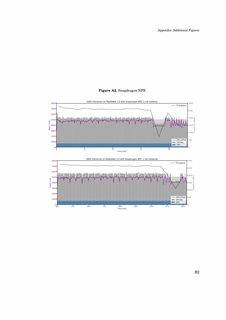
Appendix: Additional Figures

Figure A2. Snapdragon NPE

0 5 10 15 20Time (min)

0

500

1000

1500

2000

2500

3000

Freq

uenc

ies

(MH

z)

CPU LITTLECPU bigGPU

Throughput

0

1000

2000

3000

4000

5000

6000

7000

8000

Pow

er (m

W)

3000 inferences on MobileNet 1.0 with Snapdragon NPE, 1 net instance

0.0 2.5 5.0 7.5 10.0 12.5 15.0 17.5 20.0Time (min)

0

500

1000

1500

2000

2500

3000

Freq

uenc

ies

(MH

z)

CPU LITTLECPU bigGPU

Throughput

0

1000

2000

3000

4000

5000

6000

7000

8000

Pow

er (m

W)

3000 inferences on MobileNet 1.0 with Snapdragon NPE, 2 net instances

82

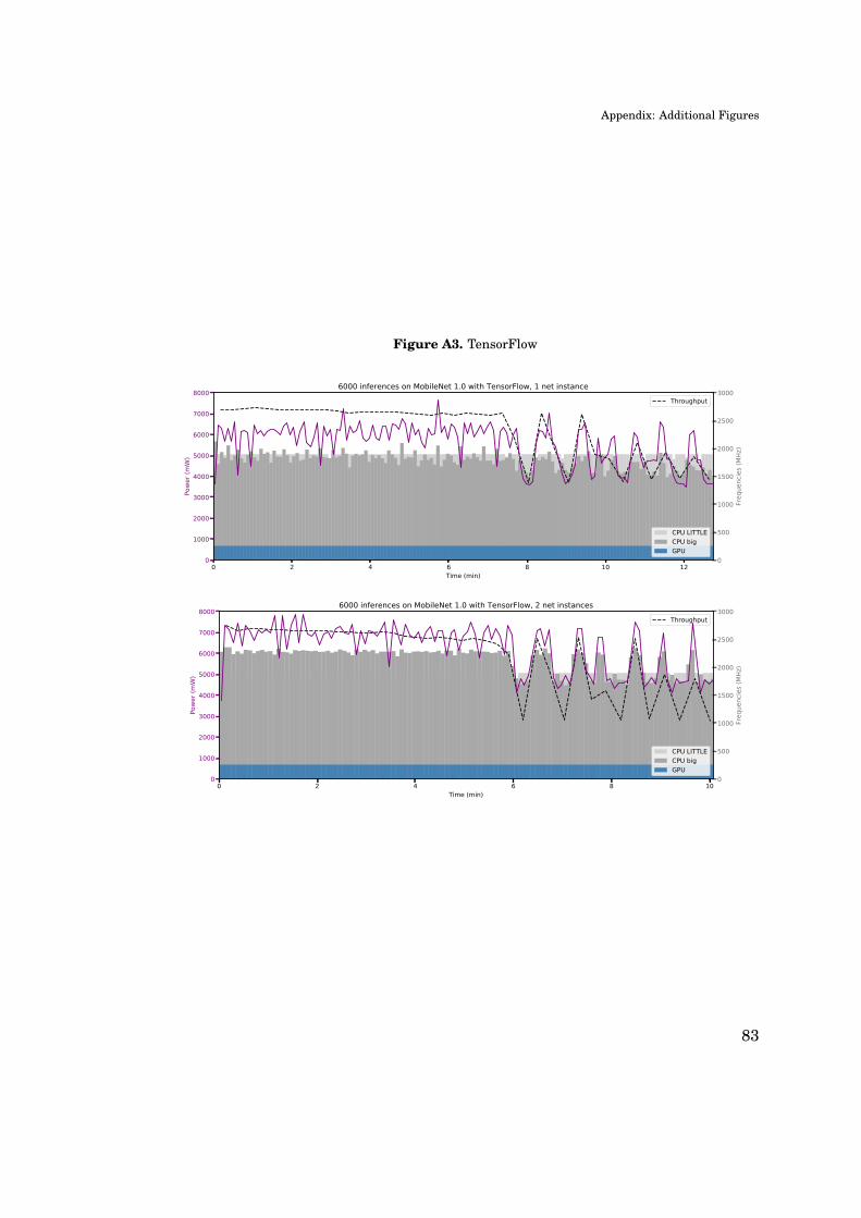
Appendix: Additional Figures

Figure A3. TensorFlow

0 2 4 6 8 10 12Time (min)

0

500

1000

1500

2000

2500

3000

Freq

uenc

ies

(MH

z)

CPU LITTLECPU bigGPU

Throughput

0

1000

2000

3000

4000

5000

6000

7000

8000

Pow

er (m

W)

6000 inferences on MobileNet 1.0 with TensorFlow, 1 net instance

0 2 4 6 8 10Time (min)

0

500

1000

1500

2000

2500

3000

Freq

uenc

ies

(MH

z)

CPU LITTLECPU bigGPU

Throughput

0

1000

2000

3000

4000

5000

6000

7000

8000

Pow

er (m

W)

6000 inferences on MobileNet 1.0 with TensorFlow, 2 net instances

83

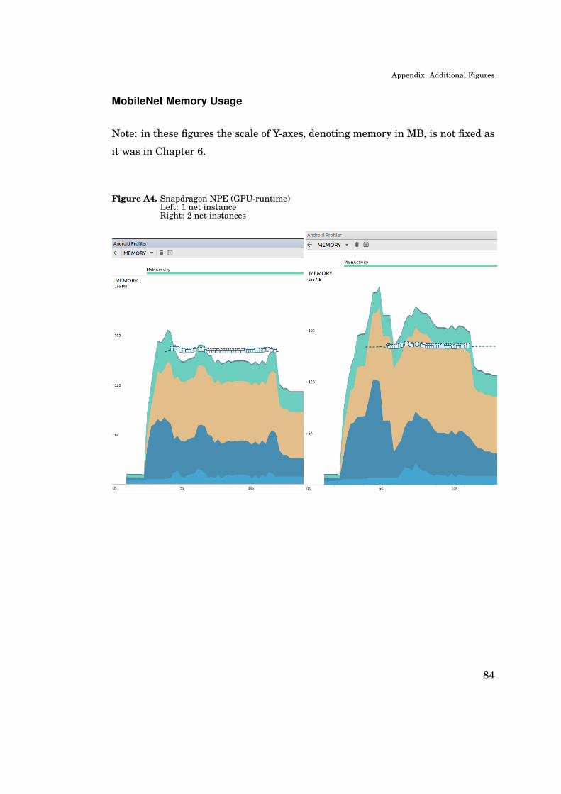
Appendix: Additional Figures

MobileNet Memory Usage

Note: in these figures the scale of Y-axes, denoting memory in MB, is not fixed as

it was in Chapter 6.

Figure A4. Snapdragon NPE (GPU-runtime)Left: 1 net instanceRight: 2 net instances

84

Appendix: Additional Figures

Figure A5. Snapdragon NPETop: 1 net instanceBottom: 2 net instances

85

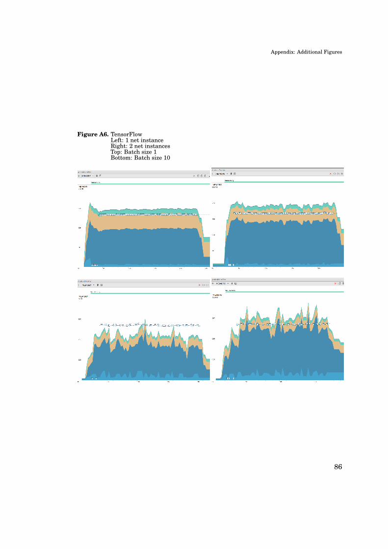
Appendix: Additional Figures

Figure A6. TensorFlowLeft: 1 net instanceRight: 2 net instancesTop: Batch size 1Bottom: Batch size 10

86