Embed Size (px)
Citation preview
Performance of Fluid-Structure Interaction based
on Analytical and Computational Techniques
A thesis submitted in fulfilment of the requirements for
for the degree of Master of Engineering
Pongpat Thavornpattanapong
BEng
Supervisor: Prof. Jiyuan Tu
Associate Supervisor: Dr. Sherman C.P. Cheung
School of Aerospace, Mechanical and
Manufacturing Engineering
RMIT University
March, 2011

c© Copyright
by
Pongpat Thavornpattanapong
2011

to my MOTHER and FATHER with love
iii
Contents
List of Tables . . . . . . . . . . . . . . . . . . . . . . . . . . . . . . . . . . ix
List of Figures . . . . . . . . . . . . . . . . . . . . . . . . . . . . . . . . . x
Abstract . . . . . . . . . . . . . . . . . . . . . . . . . . . . . . . . . . . . . xiii
Acknowledgments . . . . . . . . . . . . . . . . . . . . . . . . . . . . . . . xvi
Publications . . . . . . . . . . . . . . . . . . . . . . . . . . . . . . . . . . . xviii
Nomenclature . . . . . . . . . . . . . . . . . . . . . . . . . . . . . . . . . . xix
1 Introduction . . . . . . . . . . . . . . . . . . . . . . . . . . . . . . . . . 1
1.1 Background . . . . . . . . . . . . . . . . . . . . . . . . . . . . . . . . 1
1.2 Outline of thesis . . . . . . . . . . . . . . . . . . . . . . . . . . . . . . 8
1.3 Summary of contributions . . . . . . . . . . . . . . . . . . . . . . . . 9
2 Literature review . . . . . . . . . . . . . . . . . . . . . . . . . . . . . . 11
2.1 Frame of reference . . . . . . . . . . . . . . . . . . . . . . . . . . . . 11
2.1.1 Lagrangian frame . . . . . . . . . . . . . . . . . . . . . . . . . 11
2.1.2 Eulerian frame . . . . . . . . . . . . . . . . . . . . . . . . . . 12
2.1.3 Arbitrary Lagrangian-Eulerian frame . . . . . . . . . . . . . . 13
2.2 Fluid-structure interaction . . . . . . . . . . . . . . . . . . . . . . . . 14
2.2.1 Monolithic approach . . . . . . . . . . . . . . . . . . . . . . . 15
2.2.2 Partitioned approach . . . . . . . . . . . . . . . . . . . . . . . 15
iv
2.3 Added-mass instability in partitioned approach . . . . . . . . . . . . 20
2.4 Existing Techniques for FSI Closely Coupling . . . . . . . . . . . . . 21
2.4.1 Under-relaxation . . . . . . . . . . . . . . . . . . . . . . . . . 21
2.4.2 Reduced order models . . . . . . . . . . . . . . . . . . . . . . 23
2.4.3 Artificial compressibility . . . . . . . . . . . . . . . . . . . . . 23
2.5 Methods for computatonal mesh in FSI . . . . . . . . . . . . . . . . . 25
2.5.1 Fixed grid algorithm . . . . . . . . . . . . . . . . . . . . . . . 25
2.5.2 Moving mesh . . . . . . . . . . . . . . . . . . . . . . . . . . . 28
2.5.3 Automatic remeshing . . . . . . . . . . . . . . . . . . . . . . . 29
2.6 Summary and concluding remarks . . . . . . . . . . . . . . . . . . . . 29
3 Methodology . . . . . . . . . . . . . . . . . . . . . . . . . . . . . . . . 31
3.1 Governing equations . . . . . . . . . . . . . . . . . . . . . . . . . . . 31
3.1.1 Fluid governing equation . . . . . . . . . . . . . . . . . . . . . 31
3.1.2 Solid governing equation . . . . . . . . . . . . . . . . . . . . . 33
3.2 Discretization for governing equations . . . . . . . . . . . . . . . . . . 33
3.2.1 Discretization for fluid governing equations . . . . . . . . . . . 33
3.2.2 Discretization for solid governing equation . . . . . . . . . . . 40
3.3 Fundamental conditions for FSI coupling . . . . . . . . . . . . . . . . 42
3.4 Implementation of artificial compressibility . . . . . . . . . . . . . . . 43
3.5 Procedure of calculation . . . . . . . . . . . . . . . . . . . . . . . . . 46
3.5.1 Under-relaxation . . . . . . . . . . . . . . . . . . . . . . . . . 47
3.5.2 Aritificial compressibility . . . . . . . . . . . . . . . . . . . . . 49
3.6 Convergence of interface loads . . . . . . . . . . . . . . . . . . . . . . 52
3.7 General procedure of FSI simulation setup . . . . . . . . . . . . . . . 53
3.8 Construction and setup for mesh in FSI . . . . . . . . . . . . . . . . . 54
3.9 Summary and concluding remarks . . . . . . . . . . . . . . . . . . . . 59
4 Theoretical analysis of stability in FSI . . . . . . . . . . . . . . . . 61
4.1 Introduction . . . . . . . . . . . . . . . . . . . . . . . . . . . . . . . . 61
4.2 Simplified problem for stability analysis . . . . . . . . . . . . . . . . . 63
4.3 Theoretical analysis: under-relaxation . . . . . . . . . . . . . . . . . . 65
v
4.3.1 Stability condition: minimum numerical damping is applied . 65
4.3.2 Stability condition: maximum numerical damping is applied . 68
4.3.3 Generalization of stability condition . . . . . . . . . . . . . . . 70
4.4 Summary and concluding remarks . . . . . . . . . . . . . . . . . . . . 72
5 Validation and numerical results . . . . . . . . . . . . . . . . . . . . 75
5.1 Validation . . . . . . . . . . . . . . . . . . . . . . . . . . . . . . . . . 75
5.1.1 Geometric and material descriptions . . . . . . . . . . . . . . 76
5.1.2 Computational domain . . . . . . . . . . . . . . . . . . . . . . 76
5.1.3 Analytical solutions . . . . . . . . . . . . . . . . . . . . . . . . 76
5.1.4 Comparison between numerical and analytical solutions . . . . 78
5.2 Numerical results . . . . . . . . . . . . . . . . . . . . . . . . . . . . . 80
5.2.1 Influence of structural time integration scheme . . . . . . . . . 80
5.2.2 Influence of fluid time integration scheme . . . . . . . . . . . . 83
5.2.3 Influence of time step size . . . . . . . . . . . . . . . . . . . . 84
5.2.4 Influence of density ratio . . . . . . . . . . . . . . . . . . . . . 85
5.2.5 Influence of vessel radius . . . . . . . . . . . . . . . . . . . . . 85
5.3 Implicit solution using artificial compressibility . . . . . . . . . . . . . 87
5.4 Performance comparison . . . . . . . . . . . . . . . . . . . . . . . . . 87
5.5 Summary and concluding remarks . . . . . . . . . . . . . . . . . . . . 88
6 Fluid-structure interaction in carotid bifurcation . . . . . . . . . . 93
6.1 Abstract . . . . . . . . . . . . . . . . . . . . . . . . . . . . . . . . . . 93
6.2 Introduction . . . . . . . . . . . . . . . . . . . . . . . . . . . . . . . . 94
6.2.1 General background of atherosclerosis . . . . . . . . . . . . . . 94
6.2.2 Hypothesis on the developement of artherosclerosis . . . . . . 94
6.2.3 Types of atherosclerosis . . . . . . . . . . . . . . . . . . . . . 95
6.2.4 Clinical implications of blood pressure and heart rate . . . . . 96
6.2.5 Aim and scope . . . . . . . . . . . . . . . . . . . . . . . . . . 97
6.3 Methodology . . . . . . . . . . . . . . . . . . . . . . . . . . . . . . . 97
6.3.1 Partitioned approach for fluid-structure interaction . . . . . . 98
6.3.2 Idealistic geometry of carotid bifurcation . . . . . . . . . . . . 98
vi
6.3.3 Computational domain . . . . . . . . . . . . . . . . . . . . . . 101
6.3.4 Boundary conditions and material properties . . . . . . . . . . 101
6.3.5 Flow properties to be examined . . . . . . . . . . . . . . . . . 105
6.4 Results . . . . . . . . . . . . . . . . . . . . . . . . . . . . . . . . . . . 105
6.4.1 Healthy carotid bifurcation . . . . . . . . . . . . . . . . . . . . 105
6.4.2 Diseased carotid bifurcation – parameters affected based on
different degrees of stenosis . . . . . . . . . . . . . . . . . . . 106
6.5 Discussion . . . . . . . . . . . . . . . . . . . . . . . . . . . . . . . . . 119
6.5.1 Blood flow pattern and wall shear stress . . . . . . . . . . . . 119
6.5.2 Deformation . . . . . . . . . . . . . . . . . . . . . . . . . . . . 119
6.5.3 Principal stress . . . . . . . . . . . . . . . . . . . . . . . . . . 120
6.5.4 Relationship of pulse pressure, MD and minimum value of MPS121
6.6 Summary and concluding remarks . . . . . . . . . . . . . . . . . . . . 122
7 Concluding Remarks . . . . . . . . . . . . . . . . . . . . . . . . . . . 123
7.1 Achievements and their significances . . . . . . . . . . . . . . . . . . 123
7.1.1 Numerical and theoretical analysis on influence of structural
time integration schemes on added mass instability in FSI . . 123
7.1.2 Performance comparision between under-relaxation technique
and artificial compressibility . . . . . . . . . . . . . . . . . . . 124
7.1.3 Application of artificial compressibility to artherosclerosis in
carotid bifurcation . . . . . . . . . . . . . . . . . . . . . . . . 125
7.2 Future Work . . . . . . . . . . . . . . . . . . . . . . . . . . . . . . . . 125
Appendix A Detail derivation . . . . . . . . . . . . . . . . . . . . . . . 127
A.1 Discretization of structural acceleration . . . . . . . . . . . . . . . . . 127
A.1.1 When minimum numerical damping is applied . . . . . . . . . 127
A.1.2 When maximum numerical damping is applied . . . . . . . . . 130
A.2 Discretization of fluid acceleration . . . . . . . . . . . . . . . . . . . . 131
A.2.1 First order accurate backward Euler . . . . . . . . . . . . . . 132
A.2.2 Second order accurate backward Euler . . . . . . . . . . . . . 132
A.2.3 Trapezoidal rule . . . . . . . . . . . . . . . . . . . . . . . . . . 132
vii
Appendix B Analysis on added mass instability . . . . . . . . . . . . 133
B.1 Analysis . . . . . . . . . . . . . . . . . . . . . . . . . . . . . . . . . . 133
B.1.1 Leap-Frog and Euler scheme with under-relaxation . . . . . . 134
B.1.2 Leap-Frog and Euler scheme with artificial compressibility . . 137
B.2 Conclusion . . . . . . . . . . . . . . . . . . . . . . . . . . . . . . . . . 140
References . . . . . . . . . . . . . . . . . . . . . . . . . . . . . . . . . . . . 141
viii
List of Tables
3.1 Table of mesh motion analysis. . . . . . . . . . . . . . . . . . . . . . . 55
5.1 Influence of amplitude decay factor on the critical relaxation factor
when time step size is 0.001s. . . . . . . . . . . . . . . . . . . . . . . 83
5.2 The critical relaxation factors when time step size is 0.001s and first
order accurate backward Euler scheme is used for fluid acceleration. . 83
5.3 Influence of amplitude decay factor on required density ratio when
time step size is 0.0001s. . . . . . . . . . . . . . . . . . . . . . . . . . 84
5.4 Influence of amplitude decay factor on required density ratio when
time step size is 0.00001s. . . . . . . . . . . . . . . . . . . . . . . . . 84
5.5 The critical value of relaxation factor when using time step size is
0.001s and radius is increased to 0.7 cm . . . . . . . . . . . . . . . . . 85
5.6 Comparison between the consumed computation time when using ar-
tificial compressibility and under-relaxation technique. . . . . . . . . 89
6.1 FSI parameters, material properties and dimensions of carotid bifur-
cation used in this work . . . . . . . . . . . . . . . . . . . . . . . . . 102
ix
List of Figures
1.1 The collapse of the Tocoma narrow bridge . . . . . . . . . . . . . . . 3
1.2 Fluid-structure interaction of human blood vessel . . . . . . . . . . . 4
1.3 Fluid-structure interaction of oscillating rear windshield of convertible
car . . . . . . . . . . . . . . . . . . . . . . . . . . . . . . . . . . . . . 4
1.4 Introduction to fluid-structure interaction . . . . . . . . . . . . . . . 6
2.1 Classification of analysis types in fluid-structure interaction. . . . . . 14
2.2 Diagram of partitioned approach . . . . . . . . . . . . . . . . . . . . 16
2.3 Procedure of reduced order models for fluid-structure interaction . . . 24
3.1 Interpolation using upwind differencing scheme when Fc is greater or
equal to 0. . . . . . . . . . . . . . . . . . . . . . . . . . . . . . . . . . 36
3.2 Interpolation using upwind differencing scheme when Fc is less than 0. 36
3.3 Interpolation using central differencing scheme . . . . . . . . . . . . . 37
3.4 Diagram of FSI coupling . . . . . . . . . . . . . . . . . . . . . . . . . 44
3.5 Flowchart of standard procedure of partitioned approach when using
under-relaxation technique . . . . . . . . . . . . . . . . . . . . . . . . 47
3.6 Flowchart of standard procedure of partitioned approach when using
artificial compressibility . . . . . . . . . . . . . . . . . . . . . . . . . 50
3.7 Mesh motion of case 1. . . . . . . . . . . . . . . . . . . . . . . . . . . 56
3.8 Mesh motion of case 2. . . . . . . . . . . . . . . . . . . . . . . . . . . 57
3.9 Mesh motion of case 3. . . . . . . . . . . . . . . . . . . . . . . . . . . 58
4.1 Graphical representation of flexible vessel. . . . . . . . . . . . . . . . 64
x
4.2 Plot of 4(1+γ)
in the range of γ between zero and one. . . . . . . . . . 71
5.1 Computational meshes of fluid and solid domain. . . . . . . . . . . . 77
5.2 Relationship between pressure wave velocity and Young modulus of
flexible vessel. . . . . . . . . . . . . . . . . . . . . . . . . . . . . . . . 79
5.3 Pressure wave propagation along the flexible cylindrical vessel with
various Young modulus at 6 ms. . . . . . . . . . . . . . . . . . . . . . 81
5.4 Pressure wave propagation along the flexible cylindrical vessel with
various Young modulus at 11 ms. . . . . . . . . . . . . . . . . . . . . 82
5.5 Influence of density ratio and amplitude decay factor on the impact
of critical relaxation factor. . . . . . . . . . . . . . . . . . . . . . . . 86
6.1 Geometry of carotid bifurcation . . . . . . . . . . . . . . . . . . . . . 100
6.2 Computational grid used in this work. . . . . . . . . . . . . . . . . . 103
6.3 Flow conditions at the ends of common, internal and external carotid
artery. . . . . . . . . . . . . . . . . . . . . . . . . . . . . . . . . . . . 104
6.4 Wall shear stress at various monitoring points. The common carotid
artery (CCA), inner and outer monitoring points of the internal and
external carotid artery (ICA-in and ECA-in, and ICA-out and ECA-
out respectively). . . . . . . . . . . . . . . . . . . . . . . . . . . . . . 107
6.5 Flow pattern in carotid bifurcation with different degrees of stenosis. 109
6.6 Pattern of deformation in carotid bifurcation with different degrees
of stenosis. . . . . . . . . . . . . . . . . . . . . . . . . . . . . . . . . . 110
6.7 Identification of location of negative MPS (compression) in carotid
bifurcation with different degrees of stenosis. Note that this plot is
in logarithmic scale. The small value in this scale represents negative
MPS. . . . . . . . . . . . . . . . . . . . . . . . . . . . . . . . . . . . . 111
6.8 Contours of MPS distributions based on different degrees of stenosis. 113
6.9 Plots of the MPS on stenosis in diseased carotid bifurcations. . . . . . 114
6.10 Pattern of wall shear stress in carotid bifurcation with different de-
grees of stenosis. . . . . . . . . . . . . . . . . . . . . . . . . . . . . . 116
6.11 Plots of wall shear stress along the stenosis. . . . . . . . . . . . . . . 117
xi

6.12 Relationship of pulse pressure, MD and minimum value of MPS. . . . 118
B.1ρfµi
ρshs> 0, R > 1 (Unconditionally unstable) . . . . . . . . . . . . . . . 138
xii
Performance of Fluid-Structure Interaction based
on Analytical and Computational Techniques
Pongpat Thavornpattanapong, Bachelor of [email protected]
RMIT University, 2011
Supervisor: Prof. Jiyuan TuAssociate Supervisor: Dr. Sherman C.P. Cheung
Abstract
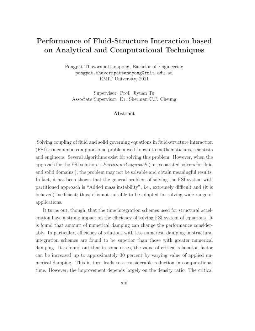
Solving coupling of fluid and solid governing equations in fluid-structure interaction
(FSI) is a common computational problem well known to mathematicians, scientists
and engineers. Several algorithms exist for solving this problem. However, when the
approach for the FSI solution is Partitioned approach (i.e., separated solvers for fluid
and solid domains ), the problem may not be solvable and obtain meaningful results.
In fact, it has been shown that the general problem of solving the FSI system with
partitioned approach is “Added mass instability”, i.e., extremely difficult and (it is
believed) inefficient; thus, it is not suitable to be adopted for solving wide range of
applications.
It turns out, though, that the time integration schemes used for structural accel-
eration have a strong impact on the efficiency of solving FSI system of equations. It
is found that amount of numerical damping can change the performance consider-
ably. In particular, efficiency of solutions with less numerical damping in structural
integration schemes are found to be superior than those with greater numerical
damping. It is found out that in some cases, the value of critical relaxation factor
can be increased up to approximately 30 percent by varying value of applied nu-
merical damping. This in turn leads to a considerable reduction in computational
time. However, the improvement depends largely on the density ratio. The critical
xiii
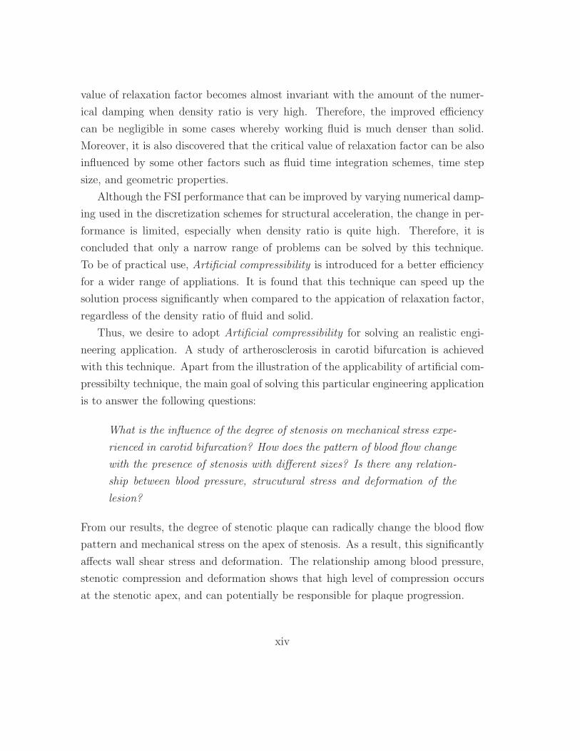
value of relaxation factor becomes almost invariant with the amount of the numer-
ical damping when density ratio is very high. Therefore, the improved efficiency
can be negligible in some cases whereby working fluid is much denser than solid.
Moreover, it is also discovered that the critical value of relaxation factor can be also
influenced by some other factors such as fluid time integration schemes, time step
size, and geometric properties.
Although the FSI performance that can be improved by varying numerical damp-
ing used in the discretization schemes for structural acceleration, the change in per-
formance is limited, especially when density ratio is quite high. Therefore, it is
concluded that only a narrow range of problems can be solved by this technique.
To be of practical use, Artificial compressibility is introduced for a better efficiency
for a wider range of appliations. It is found that this technique can speed up the
solution process significantly when compared to the appication of relaxation factor,
regardless of the density ratio of fluid and solid.
Thus, we desire to adopt Artificial compressibility for solving an realistic engi-
neering application. A study of artherosclerosis in carotid bifurcation is achieved
with this technique. Apart from the illustration of the applicability of artificial com-
pressibilty technique, the main goal of solving this particular engineering application
is to answer the following questions:
What is the influence of the degree of stenosis on mechanical stress expe-
rienced in carotid bifurcation? How does the pattern of blood flow change
with the presence of stenosis with different sizes? Is there any relation-
ship between blood pressure, strucutural stress and deformation of the
lesion?
From our results, the degree of stenotic plaque can radically change the blood flow
pattern and mechanical stress on the apex of stenosis. As a result, this significantly
affects wall shear stress and deformation. The relationship among blood pressure,
stenotic compression and deformation shows that high level of compression occurs
at the stenotic apex, and can potentially be responsible for plaque progression.
xiv
Performance of Fluid-Structure Interaction based
on Analytical and Computational Techniques
Declaration
I certify that except where due acknowledgement has been made, the work isthat of the author alone; the work has not been submitted previously, in whole orin part, to qualify for any other academic award; the content of the thesis is theresult of work which has been carried out since the official commencement dateof the approved research program; any editorial work, paid or unpaid, carried outby a third party is acknowledged; and, ethics procedures and guidelines have beenfollowed.
Pongpat ThavornpattanapongSeptember 14, 2011
xv
Acknowledgments
I would like to express my deep-felt gratitude to my advisor, Prof. Jiyuan Tu of
School of Aerospace, Mechanical and Manufacturing at Royal Melbourne Institute
of Technology at Bundoora,Melbourne, for his advice, encouragement, enduring
patience and constant support.
He was never ceasing in his belief in me (though I was often doubting in my
own abilities), always providing clear explanations when I was (hopelessly) lost,
constantly driving me with energy when I was tired, and always giving me his time,
in spite of anything else that was going on. His response to my verbal thanks one
day was a very modest, “It’s my job.” I wish all students the honor and opportunity
to experience his ability to perform at that job.
I also wish to thank my secondary supervisor, Dr. Sherman C.P. Cheung of
School of Aerospace, Mechanical and Manufacturing at Royal Melbourne Institute
of Technology at Bundoora,Melbourne. His suggestions, comments and additional
guidance were invaluable to the completion of this work.
Additionally, I want to thank Dr. Jon Watmuff and my colleages at Royal
Melbourne Institute of Technology at Bundoora,Melbourne for all their hard work
and dedication, providing me the means to complete my degree and prepare for a
career as an engineer. This includes (but certainly is not limited to) the following
individuals: Dr. Kelvin K.L. Wong, Dr. Sura Tundee, Dr. Zhang Kai, Dr. Jie
Yang.
I also want to thank the Commonwealth of Australia, through the Cooperative
Research Centre for Advanced Automotive Technology (Project: Developing Nu-
merical Model for Flow-Induced Vibration Excitation Mechanisms towards Virtual
Laboratory Simulation,C4-503) for providing funding for conductiong this research.
xvi

And finally, I must thank my dear family for putting up with me during the
development of this work with continuing, loving support and no complaint.
Pongpat Thavornpattanapong
RMIT University
March 2011
xvii
List of Publications
The followings are papers completed during this study of Master degree.
• P. Thavornpattanapong, K.K.L. Wong, S.C.P. Cheung and J.Y. Tu, 2011,
Mathematical Analysis of Added-Mass Instability in Fluid-Structure Interac-
tion, International journal of mathematics and statistics.(In press, this journal
paper is a part of Appendix B)
• P. Thavornpattanapong, S.C.P. Cheung, K.K.L. Wong and J.Y. Tu, 2011,
Fluid structure interaction applied to carotid bifurcation flow, Journal of Me-
chanics in Medicine and Biology.(Minor revision, this journal paper is a part
of from Chapter 6)
• K.K.L. Wong, P. Thavornpattanapong, S. C.P. Cheung, Zhonghua Sun
, Stephen Grant Worthley, and J.Y. Tu , 2011, Influence of Calcification
Agglomerate on Plaque Vulnerability in Atherosclerotic vessels, Annals of
Biomedical Engineering.(Submitted)
• K.K.L. Wong, P. Thavornpattanapong, T. Chaichana, Z. Sun, and J.Y.
Tu, 2010, Analysis on Intra-aneurysmal Flow Influence By Stenting, The 3rd
International Conference on BioMedical Engineering and Informatics (BMEI
2010), Paper ID: P0612, Yantai, China.
xviii
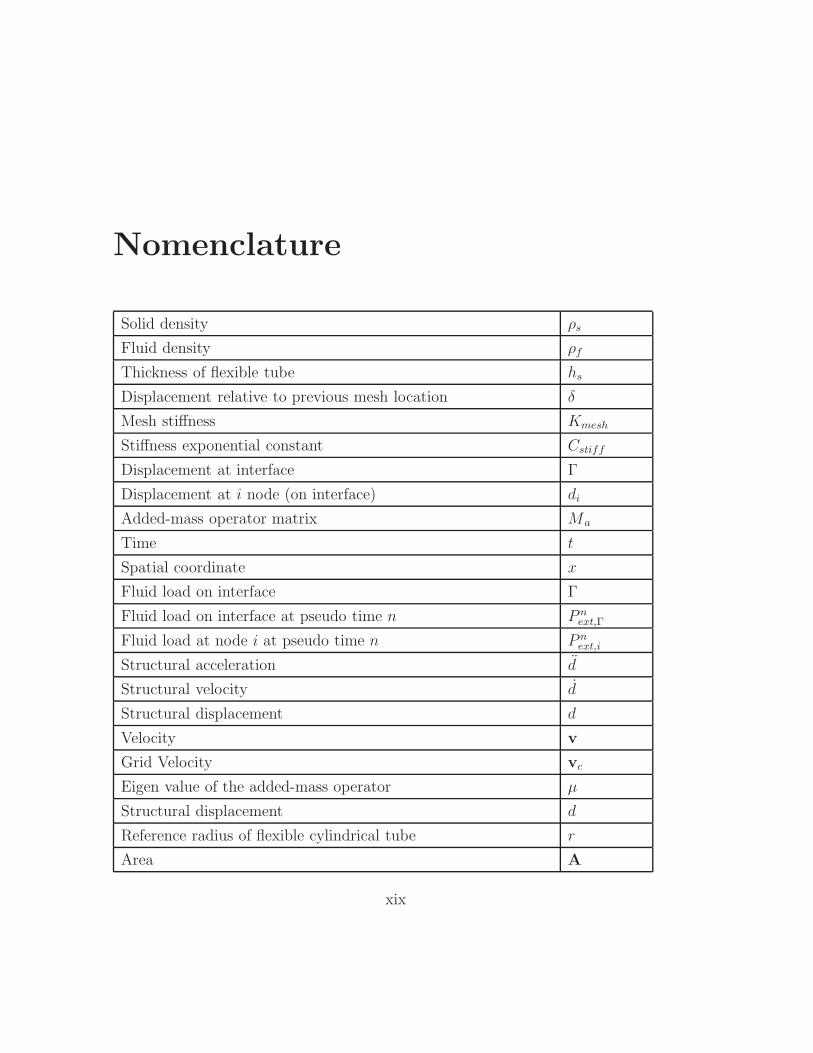
Nomenclature
Solid density ρs
Fluid density ρf
Thickness of flexible tube hs
Displacement relative to previous mesh location δ
Mesh stiffness Kmesh
Stiffness exponential constant Cstiff
Displacement at interface Γ
Displacement at i node (on interface) di
Added-mass operator matrix Ma
Time t
Spatial coordinate x
Fluid load on interface Γ
Fluid load on interface at pseudo time n P next,Γ
Fluid load at node i at pseudo time n P next,i
Structural acceleration d
Structural velocity d
Structural displacement d
Velocity v
Grid Velocity vc
Eigen value of the added-mass operator µ
Structural displacement d
Reference radius of flexible cylindrical tube r
Area A
xix
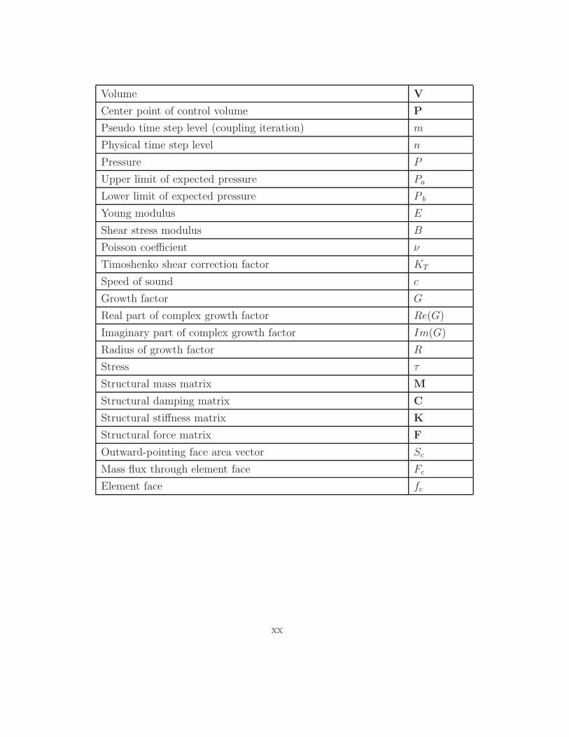
Volume V
Center point of control volume P
Pseudo time step level (coupling iteration) m
Physical time step level n
Pressure P
Upper limit of expected pressure Pa
Lower limit of expected pressure P b
Young modulus E
Shear stress modulus B
Poisson coefficient ν
Timoshenko shear correction factor KT
Speed of sound c
Growth factor G
Real part of complex growth factor Re(G)
Imaginary part of complex growth factor Im(G)
Radius of growth factor R
Stress τ
Structural mass matrix M
Structural damping matrix C
Structural stiffness matrix K
Structural force matrix F
Outward-pointing face area vector Sc
Mass flux through element face Fc
Element face fc
xx
Chapter 1
Introduction
1.1 Background
In past decades, significant improvement in development and use of numerical sim-
ulation for solving fluid and solid engineering problems has been achieved. Many
specialized techniques (such as turbulent models in fluid mechanics and structural
mechanic models for composite material) have been proposed to realistically model
complex flows and structural mechanical behaviours. In addition, the advance of
computational science has enabled the computer to become more valuable and effi-
cient for analyzing many real world engineering applications. With this tremendous
computating power, we reached the stage where not only fluid or solid problems
can be numerically solved, but also the interaction between the two states, which
are important when it comes to analysing complex phenomenon. The method of
solving interaction between fluid and solid is generally called Fluid-Structure In-
teraction (FSI), which is also known as Flow Induced Vibration Excitation (FIV).
These are used in automotive, aerospace and biomedical engineering applications
such as hydraulic engine mount, oscillation of rear windshield of the convertible car,
vibration of marine riser as well as blood-vessel flow. The important engineering
applications which require FSI analysis are
1
2 CHAPTER 1. INTRODUCTION
• Automotive engineering: Analysis of airbag deployment (e.g. Sinz and Her-
mann, 2008), analysis of hydraulic engine mount (e.g. Daneshmand et al.,
2005; Shangguan and Lu, 2004), analysis of roof of the convertible car (e.g.
Knight et al., 2010), analysis of tyre hydroplaning (e.g. Cho et al., 2006);
• Aerospace engineering: Analysis of wing flutter (e.g. Eloy et al., 2007; Silva
and Bartels, 2004; Storti et al., 2009; Dang et al., 2010);
• Biomedical engineering: Analysis of atherosclerosis (e.g. Tang et al., 2008;
Tada and Tarbell, 2005; Samuel et al., 2008; Thubrikar and Robicsek, 1995;
Lee and Xu, 2002), analysis of heart disease (e.g. Nobili et al., 2008; Lau
et al., 2010; Hart et al., 2003; Xia et al., 2009; Hart et al., 2003);
• Civil engineering: Analysis of high rise building (e.g. Braun and Awruch,
2009), analysis of long bridge (e.g. Bai et al., 2010; Sun et al., 2008), analysis
of marine riser (e.g. Borazjani et al., 2008; Sagatun et al., 2002; Yamamoto
et al., 2004);
In these applications, the most challenging task is to deal with large deformation
of solid structures which interact with highly complex flows. A good example is the
Tocoma bridge disaster which happened in 1940 as shown in Figure 1.1.
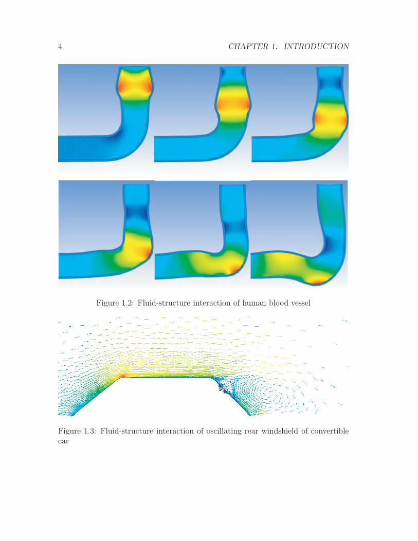
The second example is the large deformation, which occurs due to interaction
between organic tissue of human blood vessel and the pressurized blood flow. This
can be seen in Figure 1.2
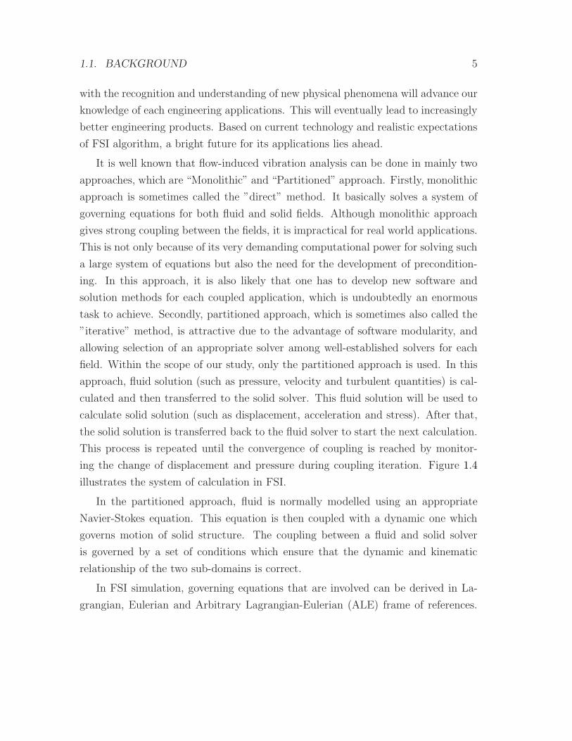
Another important engineering application of FSI is the oscillation of the con-
vertible car roof. The performance of the roof is influenced by FSI between the
canopy and flow over the roof. The interaction between the canopy and surrounding
flow field is a necessary component of a realistic convertible roof simulation and the
ability to solve it is recognized as an important challenge of the automotive research
community. The vortical flow surrounding the roof and the dynamics of the roof
structure at a specific point of time during simulation is shown in Figure 1.3
Numerical analyses of engineering applications are highly important to industrial
success. This is because the interplay between numerical FSI simulation and analysis
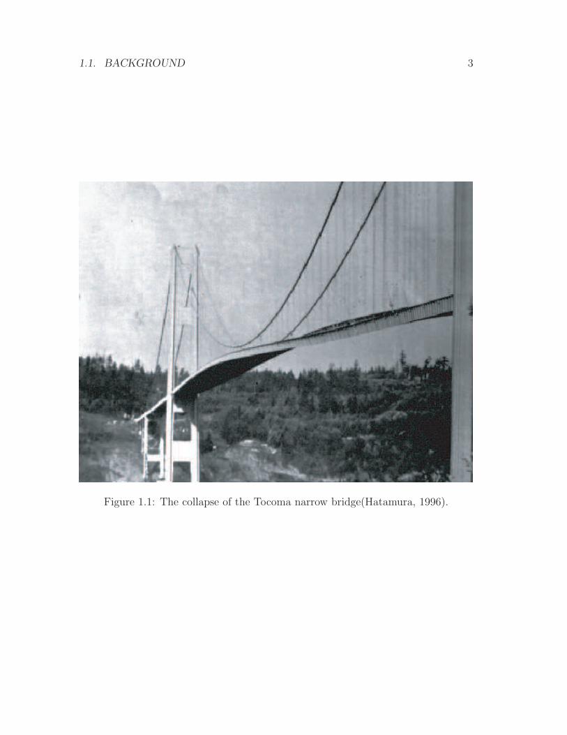
1.1. BACKGROUND 3
Figure 1.1: The collapse of the Tocoma narrow bridge(Hatamura, 1996).
4 CHAPTER 1. INTRODUCTION
Figure 1.2: Fluid-structure interaction of human blood vessel
Figure 1.3: Fluid-structure interaction of oscillating rear windshield of convertiblecar
1.1. BACKGROUND 5
with the recognition and understanding of new physical phenomena will advance our
knowledge of each engineering applications. This will eventually lead to increasingly
better engineering products. Based on current technology and realistic expectations
of FSI algorithm, a bright future for its applications lies ahead.
It is well known that flow-induced vibration analysis can be done in mainly two
approaches, which are “Monolithic” and “Partitioned” approach. Firstly, monolithic
approach is sometimes called the ”direct” method. It basically solves a system of
governing equations for both fluid and solid fields. Although monolithic approach
gives strong coupling between the fields, it is impractical for real world applications.
This is not only because of its very demanding computational power for solving such
a large system of equations but also the need for the development of precondition-
ing. In this approach, it is also likely that one has to develop new software and
solution methods for each coupled application, which is undoubtedly an enormous
task to achieve. Secondly, partitioned approach, which is sometimes also called the
”iterative” method, is attractive due to the advantage of software modularity, and
allowing selection of an appropriate solver among well-established solvers for each
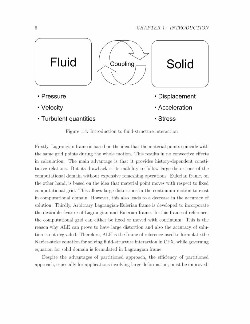
field. Within the scope of our study, only the partitioned approach is used. In this
approach, fluid solution (such as pressure, velocity and turbulent quantities) is cal-
culated and then transferred to the solid solver. This fluid solution will be used to
calculate solid solution (such as displacement, acceleration and stress). After that,
the solid solution is transferred back to the fluid solver to start the next calculation.
This process is repeated until the convergence of coupling is reached by monitor-
ing the change of displacement and pressure during coupling iteration. Figure 1.4
illustrates the system of calculation in FSI.
In the partitioned approach, fluid is normally modelled using an appropriate
Navier-Stokes equation. This equation is then coupled with a dynamic one which
governs motion of solid structure. The coupling between a fluid and solid solver
is governed by a set of conditions which ensure that the dynamic and kinematic
relationship of the two sub-domains is correct.
In FSI simulation, governing equations that are involved can be derived in La-
grangian, Eulerian and Arbitrary Lagrangian-Eulerian (ALE) frame of references.
6 CHAPTER 1. INTRODUCTION
Fluid Solid
• Pressure
• Velocity
• Turbulent quantities
• Displacement
• Acceleration
• Stress
Coupling
Figure 1.4: Introduction to fluid-structure interaction
Firstly, Lagrangian frame is based on the idea that the material points coincide with
the same grid points during the whole motion. This results in no convective effects
in calculation. The main advantage is that it provides history-dependent consti-
tutive relations. But its drawback is its inability to follow large distortions of the
computational domain without expensive remeshing operations. Eulerian frame, on
the other hand, is based on the idea that material point moves with respect to fixed
computational grid. This allows large distortions in the continuum motion to exist
in computational domain. However, this also leads to a decrease in the accuracy of
solution. Thirdly, Arbitrary Lagrangian-Eulerian frame is developed to incorporate
the desirable feature of Lagrangian and Eulerian frame. In this frame of reference,
the computational grid can either be fixed or moved with continuum. This is the
reason why ALE can prove to have large distortion and also the accuracy of solu-
tion is not degraded. Therefore, ALE is the frame of reference used to formulate the
Navier-stoke equation for solving fluid-structure interaction in CFX, while governing
equation for solid domain is formulated in Lagrangian frame.
Despite the advantages of partitioned approach, the efficiency of partitioned
approach, especially for applications involving large deformation, must be improved.
1.1. BACKGROUND 7
This is because of the “added mass effect” instability. This instability usually occurs
in problems with large deformation and light weight structure. The main reason
why this instability exists in the FSI solution system is the lack of implicitness
of FSI solution algorithm of partitioned approach. Information which is used for
calculating FSI solution in this approach only comes from the solution of the previous
coupling step. This makes the solution explicit and likely to fail. To eliminate this
instability, there are many developed techniques available. The most widely used
technique is the application of under-relaxation factors. By using this technique,
small values of coupling relaxation factors of interface loads must be used. This
leads to a significant increase in computational time. Therefore, it is not suitable
for industrial usage where time is of importance. Other techniques are “reduced
order model” and accelerators (Aitken’s or Steepest descent). However, to the best
of our knowledge, none of these techniques is used in existing commercial software
(such as ANSYS) which can efficiently improve the stability of FSI system for a
wide range of engineering applications. Therefore, it is important that an efficient
method must be developed so that FSI simulation can be conducted efficiently and
conveniently by engineers in various industries.
Four main objectives are accomplished in the thesis. The first aim of the re-
search is to derive theoretical proof of the existence of added-mass instability in
fluid structure interaction. This mathematical analysis can also indicate important
parameters, which significantly influence the stability of FSI simulation. Secondly,
an efficient technique for analysing real world engineering applications is developed
based on the information obtained from the mathematical analysis. Thirdly, cre-
ation of an add-on code is achieved by constructing a user routine in FORTRAN
language to work internally with CFX. This allows an additional capability to the
commercial software to handle instability of fluid-structure interaction. The tech-
nique implements the idea of artificial compressibility. It is validated with well
defined numerical and physical experiments. The last objective of the research is to
compare the performance of artificial compressibility to the under-relaxation tech-
nique. This is done by considering the time consumption for simulating the same
physical phenomenon with different techniques.
8 CHAPTER 1. INTRODUCTION
The four main objectives of this work can be summarized as follows:
• To provide a theoretical analysis of added-mass instability that focuses on
improving the performance of FSI using the partitioned approach;
• To develop an efficient and stable tool to analyze applications that are relevant
to FSI;
• To validate the techniques with well defined analytical solutions;
• To evaluate the performance of artifical compressibility and compare it to the
under-relaxation technique.
1.2 Outline of thesis
The contents of the remaining six chapters are as follows. In Chapter 2, the basic
concepts of FSI are reviewed. The fundamental knowledge of FSI, such as the de-
scription of monolithic and partitioned approach as well as frame of reference in con-
tinuum are explained. Next, the existence of added-mass instability in partitioned
approach is discussed. This is followed by the review of the existing techniques for
treating the instability, i.e. the under-relaxation factors and artificial compressibil-
ity. The literature review also covers other important topics in FSI such as fixed
grid algorithm and automatic remeshing.
Chapter 3 governing equations and discretization schemes are presented. Next,
the fundamental conditions for FSI coupling, namely dynamic and kinematic, are
discussed, followed by the implementation of artificial compressibility is explained.
Then, the description of computing procedure with under-relaxation factors and
artificial compressibiltiy are described. In addition, the best practices and general
procedure of simulation set up and construction of computation meshes in ANSYS-
CFX, which are used throughout this project, are provided.
Chapter 4 addresses the theoretical analysis of added-mass instability in fluid-
structure interaction. Firstly, the instability of fluid-structure interaction calculation
1.3. SUMMARY OF CONTRIBUTIONS 9
that utilizes the generalized-α time integration schemes involving minimum numer-
ical damping and backward Euler schemes are described. Then, a similar analysis
of instability of fluid-structure interaction calculation that employs the generalized-
α time integration schemes involving minimum numerical damping and backward
Euler schemes are discussed.
Chapter 5 covers validations and numerical results that are used to confirm the
validity of theoretical analysis provided in Chapter 4. The validations are conducted
against well-defined analytical solutions of the wave-propagation along a flexible
tube. The numerical results are presented to prove the influence of amplitude decay
factor, time step size, density ratio and geometric properties of the FSI problem when
the under-relaxation technique is used. This is then followed by the demonstration
of the efficiency of the under-relaxation technique and compare its perfomance with
the artificial compressibility.
In Chapter 6, the utilization of artificial compressibility to real world engineering
applications are presented. A FSI study of atherosclerosis in carotid bifurcation is
presented in order to demonstrate the applicability of our method.
Finally, the concluding remarks are made in Chapter 7. Further research direc-
tion is also suggested.
1.3 Summary of contributions
• An intensive investigation of the influence of numerical damping in
structural discretization schemes on the instability of FSI coupling
by using theoretical and numerical tools. The outcome of this provides
researchers an understanding of the impact of numerical schemes and therefore
can help them to conduct FSI numerical experiments in a more efficient way
in the future.
• Performance comparision between under-relaxation technique and
artificial compressibility. It is shown in this work by comparing requried
10 CHAPTER 1. INTRODUCTION
computational time of each technique that the performance of artificial com-
pressibility is considerably superior than that of under-relaxation technique.
• A study of fluid-structure interaction of atherosclerosis in carotid
bifurcation. The results of the study can be used as a platform for future
work in atherosclerotic researches aiming for thoroughly understanding the
complicated process of the disease.
Chapter 2
Literature review
In this chapter, we provide a brief introduction to the theory of fluid-structure
interaction(FSI) and necessary prerequsite for the rest of this thesis.
2.1 Frame of reference
Numerical modelling of continuums often involves discretization of these multi-
dimensional domains into finite grids. Each grid satisfies the relevant equations
governing the kinematics of the continuum. Fundamental to these governing equa-
tions are how the continuum distortions are related to the computational grids.
The followings are types of reference frame used for describing the kinematic of the
continuum:
• Lagrangian frame;
• Eulerian frame;
• Arbitrary Lagrangian-Eulerian frame.
2.1.1 Lagrangian frame
By using Lagrangian frame of reference, computational grids deform completely fol-
lowing the distortion of the continuum material. This implies that the convective
11
12 CHAPTER 2. LITERATURE REVIEW
term is negligible (Price, 2006), and the computational demand can be greatly re-
duced. The reason for this is that a partial derivative with respect to time, which
represents the rate of change observed at a grid node in space, becomes zero since
the material particle is strictly followed by the computation node. This also links to
another advantage which is its ability to do a precise tracking of material position
in the continuum. In other words, the exact displacement of the deforming grid
is defined. This advantage comes with the inability to handle large material dis-
tortion in continuum. Therefore, it is commonly used in solid analysis rather than
fluid analysis where large distortion of material in continuum often occurs because
fluid particles are not strongly bonded together and tend to move in highly chaotic
ways in space. However, it can be useful for describing fluid flows with compli-
cated free surface structure whereby the free surface boundary must be accurately
determined. Ramaswamy et al. (1986) modeled fluid domain using this frame of
reference such that the computational grid moves with fluid particles. By using this
method, large displacement of the mesh can inevitably occur, but this problem can
be handled by adopting automatic rezoning techniques. Another difficulty that arises
when using Lagrangian frame is that during calculation, the volume of each finite
element must be constant since the grids moves with fluid particles and the element
boundary changes in a way that fluid inside each element remains unchanged. This
constraint can be satified by employing a velocity correction procedure introduced
by Chorin (1968). Similar approaches can be found in numerous works (Schneider
et al., 1978; Mizukami and Tsuchiya, 1984; Kawahara and Ohmiya, 1985; Kawahara
and Ohmiya, 1985; Hirt et al., 1970). Hirt et al. (1970) conducted a computational
stability analysis of this correction method and found that timestep size, the surface
tension coefficient, fluid density, the volume and width of the surface cells are the
important parameters that restrictively determine the success of this method.
2.1.2 Eulerian frame
By using Eulerian frame of reference, computational grids are fixed in space and
the continuum deforms with respect to the grids (Shabana, 2008). This means that
2.1. FRAME OF REFERENCE 13
the rate of change observed at a fixed grid node in space is nonzero and therefore
the convective term cannot be ignored, unlike that in Lagrangian frame (Jacobson,
1999; Donea et al., 2004). Its main advantage is the ability to handle large distortion
of material in continuum. This is because the grids remain unchanged throughout
calculation and the mass conservation is forced by checking the balance of fluxes at
surfaces of each elements (Carlton, 2004). However, its drawback is the inability
of material tracking of interfaces and boundary in continuum as mentioned above.
Therefore, it is commonly used in pure fluid analysis whereby continuum can be
significantly distorted due to strong vortical flow.
2.1.3 Arbitrary Lagrangian-Eulerian frame
In FSI, Arbitrary Lagrangian-Eulerian(ALE) frame of reference has been increas-
ingly popular and detailed infomation can be found in numerous studies (Richter
and Wick, 2010; Souli et al., 2000; Zhang and Hisada, 2001; Takashi, 1994; Boffi and
Gastaldi, 2004). The ALE computational grids are allowed to move arbitrarily rela-
tive to the material deformation. This characteristic gives both the precise material
tracking and also the ability to handle large distortion of material in the contin-
uum (Donea et al., 2004). The FSI interface can be tracked accurately whereby the
computational nodes move completely with their material particles. It follows that
ALE frame is reduced to Lagrangian frame at the interface. On the contrary, the
interior computational nodes of fluid domain move arbitrarily according to the mesh
adaption methods which will be mentioned later in this chapter. For these interior
nodes, the ALE description is used and the grid velocity is taken into account when
evaluating the relative fluid velocity at moving nodes. However, in some cases, it
is possible that there may be some regions in fluid domain where computational
nodes do not move at all. In these regions, it is arguable that the ALE form of the
governing equation is reduced to the Eulerian form. The formula of fluid transport
equation in the established Eulerian differential form of the mass and momentum
conservation equations in fluid dynamics can readily be recast into the ALE form
as can be found in the work of Donea et al. (2004). The main disadvantage of ALE
14 CHAPTER 2. LITERATURE REVIEW
frame is the limitation of having large deformation of structure which leads to folded
mesh in fluid mesh while there is no such limitation when using Eulerian frame be-
cause the grid is fixed and the deformed FSI interface does not directly attach to the
computational nodes as studied by (Richter and Wick, 2010). A number of methods
for handling this limitation will be discussed later in this chapter.
2.2 Fluid-structure interaction
There are two main approaches to solving problems in fluid-structure interaction as
follows:
• Monotithic approach;
• Partitioned approach.
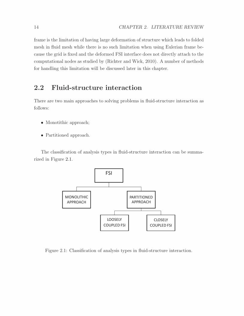
The classification of analysis types in fluid-structure interaction can be summa-
rized in Figure 2.1.
FSI
MONOLITHIC
APPROACH
PARTITIONED
APPROACH
LOOSELY
COUPLED FSI
CLOSELY
COUPLED FSI
Figure 2.1: Classification of analysis types in fluid-structure interaction.
2.2. FLUID-STRUCTURE INTERACTION 15
2.2.1 Monolithic approach
Monolithic approach is sometimes called the “direct” method. Monolithic fluid-
structure interaction simulations are solved where both fluid and solid domain are
formulated in a single system of equations (Rifai et al., 1999; Bletzinger et al., 2006;
Wood et al., 2008). This characteristic of monolithic approach allows the system to
be solved without the occurance of added-mass instability since the system is fully
coupled and solved in a single iteration loop with consistent time integration schemes
for both domains (Bendiksen, 1991; Alonso and Jameson, 1994; Grohmann et al.,
1997). In the work done by Blom (1998), a simple piston problem is used to analyse
the stability of the coupling. The consistency in time integration in monolithic solver
has proven to provide the ability to avoid numerical energy production which may
lead to the failure of the solution.
Although monolithic approach gives strong coupling between the fields, it is
commonly considered to be impractical for real world applications. This is because
it is also unlikely that one has to develop new software and solution methods for
each coupled applications, which is undoubtedly an enormous task to be achieved.
Moreover, it is not practical for industrial purposes due to time constraints. It
also demands enormous computational power for solving such a large system of
equations since it has to incorporate the behaviour of both fluid flow and solid
structure. Additionally, further development of preconditioning is still needed since
the formulation of a single equation system may result in an ill-conditioned system
matrix which includes zero entries on the diagonal (Hubner et al., 2004). Further
information of monolithic approach can be found in the work by Michler et al.
(2004).
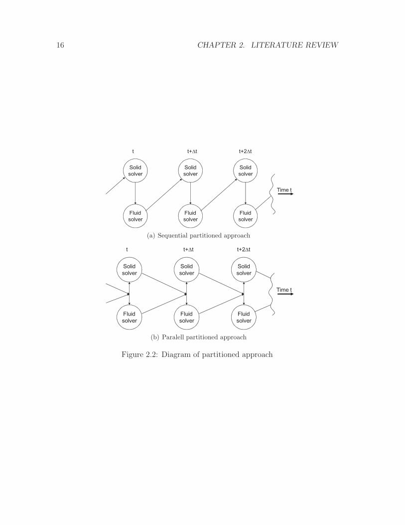
2.2.2 Partitioned approach
Another approach to fluid-structure interaction is to use two distinct solvers to model
both fluid and solid domains (Matthies et al., 2006). This technique allows the cou-
pling of the fluid and solid solution by applying coupling iterations. Some common
16 CHAPTER 2. LITERATURE REVIEW
Solid
solver
Fluid
solver
Solid
solver
Fluid
solver
Solid
solver
Fluid
solver
t t+∆t t+2∆t
Time t
(a) Sequential partitioned approach
Solid
solver
Fluid
solver
Solid
solver
Fluid
solver
Solid
solver
Fluid
solver
t t+∆t t+2∆t
Time t
(b) Paralell partitioned approach
Figure 2.2: Diagram of partitioned approach
2.2. FLUID-STRUCTURE INTERACTION 17
coupling algorithms were suggested by numerous studies (Piperno et al., 1995; Fe-
lippa et al., 2001; Farhat and Lesoinne, 2000) as shown in Figure 2.2. This soluiton
coupling allows the reuse of existing codes that have been developed for each field.
By coupling two distinct solvers, only interface information is transferred between
codes as suggested by Wood et al. (2008). Figure 2.2(a) presents the sequential
partitioned approach whereby only one solver is executed at a particular time in
sequential manner. Figure 2.2(b) demonstrates the paralell type of partitioned ap-
proach where both solvers are run simultaneously. More information about how
solid and fluid domains can be coupled in partitioned approach can be found in the
work by Felippa et al. (2001). This flexible modularity treatment of partitioned
approach is the main reason why it becomes increasingly popular in fluid-structure
interaction (Badia et al., 2008). Partitioned approach can be categorized into two
main categories, namely the Loosely and Closely coupling.
Loosely coupling
For loosely coupling. the fluid and solid load are transfered only at the end of the
solution or each time step (Felippa and Park, 1980; Masud and Hughes, 1997; Farhat
and Lesoinne, 2000). This could mean that the convergence of interface load is not
ensured. Degroote et al. (2010) suggests that the equilibrium of FSI interface within
a time step is not enforced in FSI simulation, which employs loosely coupling. Speed
of calculation using this method is very high as there is no iteration of the coupling.
However, its accuracy and stability can be very poor if the problem being solved has
strong interaction between fluid and solid as suggested by Guidoboni et al. (2009)
and l Farhat et al. (2006). This method has been widely used in problems (such as
wing fluttering), which involve light compressible flow and stiff solid structure. This
is because these problems do not have strong interaction between fluid and solid.
The main disadvantage of loosely coupled is the loss of conservation properties
of the FSI continuum. That is, it maintains some conservation properties in only
asymptotic sense such as the compatibility of fluid and solid mesh at the interaction
interface. Even though the force and displacement between fluid and solid domain
can be transferred with a very minimal loss, the energy in solution system and this
18 CHAPTER 2. LITERATURE REVIEW
method is not perfect energy conservation. Its inability to conserve energy has been
proven by various works such as those by Piperno (1997), Piperno (2001), Piperno
et al. (1995), Farhat et al. (1998) and Michler et al. (2004). It is believed that
the use of different discretization schemes (due to the difference in time and length
scale) for fluid and solid domain is the key factor that leads to the failure in con-
serving energy. It is shown by Michler (2005) that trapezoidal rule can be used in
solid analysis to yield a perfectly energy conserved solution but it cannot be used
to provide energy conserved FSI. They suggest that this problem can be eliminated
by adopting a new discretization scheme which is introduced by van Brummelen
et al. (2003) as a time-discontinuous Galerkin discretization. They categorizes this
new discretization scheme as conservative type and the trapezoidal rule as non-
conservative type. In their work, the coupling between trapezoidal rule for solid
solution and the time-discontinuous Galerkin discretization for fluid solution was
compared to the coupling, which uses the time-discontinuous Galerkin discretiza-
tion for both fluid and solid solution, was compared both in term of accuracy and
stability. By doing this, it is concluded that the solution of the conservative kind is
superior to that of the non-conservative in term of accuracy. They also show that
the solution of the non-conservative type eventually results in numerical instability
and failure. In particular, the coupling between trapezoidal rule for solid solution
and the time-discontinuous Galerkin discretization for fluid solution was compared
to the coupling which uses the time-discontinuous Galerkin discretization for both
fluid and solid solution. Moreover, it has also been suggested that the error caused
by this deficiency of loosely coupled method can be sometime reduced by improving
predictors (Piperno, 1997; Piperno, 2001). By using the predictor, the solution of
fluid is not calculated based on the old definition of interface boundary but is calcu-
lated based on the prediction made by the predictors. These predictors are normally
derived from the extrapolation of the interface deformation of previous time steps.
Furthermore, Jaiman (2007) introduces the combined interface boundary condi-
tion (CIBC) method for improving the energy conservation property of the loosely
coupled method. The key idea of this new method is to correct the interface loads
which, in loosely coupled method; some important physical processes are neglected
2.2. FLUID-STRUCTURE INTERACTION 19
due to the deficiency of the coupling condition. By correcting these interface loads,
the physical processes is introduced back to the solution system explicitly by addi-
tional calculation of correction terms. The formula for these correction terms are
derived from the calculation of the residual term in local discrete energy-preserving
equations. These equations represent the energy conservation between the dynamic
and kinematic coupling condition. That is the residual of these equations determine
the contribution of the neglected processes by the nature of conventional loosely
coupled method. In the same work, the CIBC is validated against analytical solu-
tion of the motion of elastic piston in a close domain. The solution of CIBC agrees
very well with the analytical one and is superior to that of the conventional loosely
coupled method which is very poorly calculated in terms of accuracy.
Closely coupling
For closely coupling, the fluid and solid system are solved separately in succession.
The solution of each system is transfered across the interface at the end of a stagger
iteration, which is executed many times until convergence is reached (Kalro and
Tezduyar, 2000; Tallec and Mouro, 2001; Wang and Yan, 2010). The main advantage
of this method is the high accuracy of solution. This method is recommended for
solving problems, which have strong interaction between fluid and solid. However, its
disadvantage is the slow speed of calculation since many stagger iterations together
with small under-relaxation values are needed to achieve convergence (Formaggia
et al., 2001; Jarvinen et al., 2001). Moreover, numerical instability can cause the
solution to fail if an approprite treatement is not applied.
In closely coupled method, at least two coupling iterations are needed. The
explanation to this is that with only one coupling iteration, the numerical error is
very small for one solution module only but not for the other solution module and
the interface.
The predictors, which are used in loosely coupled method, are also used in closely
coupled method but as an initialization of a new coupling iteration and not only
a new time step. It is claimed by van Brummelen and de Borst (2005) that the
introduction of a predictor into the closely coupled method can reduce the number
20 CHAPTER 2. LITERATURE REVIEW
of coupling interactions required for reaching convergence for good accuracy. van
Brummelen and de Borst (2005) concludes that the numerical effort for solving FSI
with the closely coupled method is strongly dependent on the order of extrapola-
tion of the predictor and discretization error. The discretization error is used as
a indicator if the iteration of coupling should continue. If the evaluated numerical
error is less than the discretization error, then it means that there is no additional
error introduced by coupling’s numerical instability augmented to the original error
from discretization. So, if the order of discretization error is high, then the required
number of coupling iteration can be higher. In contrast, the predictors act as a
tool to help reduce the initial value of numerical error such that a smaller number
of iterations are required for it to become lower than or equal to the value of dis-
cretization error. So it is believed that the higher the extrapolation order of the
predictor, the smaller the number of coupling iteration needed to be done. In the
work of van Brummelen and de Borst (2005), it is specifically determined that the
number of coupling iterations is equal to 2 plus the order of predictor minus the
order of the discretization error. Although the closely coupled method in theory can
allow good stability since it is designed to reduce the numerical error due to coupling
but in practice, it is found that the cost of implementing this method is normally
exceptionally high. It is claimed by Felippa et al. (2001), ”interfield iteration (cou-
pling iteration) generally costs more than cutting the time step to attain the same
accuracy level”. To the best of our knowledge, we cannot agree with this statement.
It has been proven by Causin et al. (2005) both numerically and theoretically that
the reduction in time step size may cause a more severe instability. This finding is
also confirmed by our results which will be discussed in the later chapters. However,
it is possible that the cost of the method can be reduced by applying acceleration
such as Krylov, Aitken and Steepest descent.
2.3 Added-mass instability in partitioned approach
In this section, a brief background of added-mass instability in partitioned approach
is discussed. Detailed mathematical analysis of this instability can be found in
2.4. EXISTING TECHNIQUES FOR FSI CLOSELY COUPLING 21
Chapter 3. We provide some knowledge here to help readers understand its signifi-
cance to FSI simulation. In partition approach, there are several observations about
stability of partitioned approach FSI made by Forster et al. (2007) as follows:
• Stability of FSI solution tends to be highly severe when density ratio between
fluid and solid is high;
• The increase in fluid viscosity leads to the decrease in stability. In contrast,
the increase in structural stiffness results in more stability;
• Temporal discretisation schemes used for FSI calculation can influence condi-
tion of instability;
• The decrease in time step size used for FSI calculation give an earlier occurance
of instability.
We emphasize that this instability does not occur because of the large time
step size used in calculation, which is the usual problem in CFD and FEA. Rather,
small value of time step size causes problem in FSI. This is because small time
step size can lead to large eigenvalues of the amplification operator of the explicit
step (Forster et al., 2007). This is confirmed by mathematical analysis (Causin
et al., 2005). Added-mass stability can have a significant effect on the perfomance
of FSI calculation. Computational time is increased significantly if a final solution
can reached at all. This is because solution tends to fail and solution on either fluid
or solid domain is terminated without reaching a final solution.
2.4 Summary of Existing Techniques for FSI Closely
Coupling
2.4.1 Under-relaxation
Under-relaxation technique can be used to enhance stability of solution. It is applied
to fluid and structural load transferred across FSI interface. It generally dampens
22 CHAPTER 2. LITERATURE REVIEW
the interface loads such that stability requirement of both solid and fluid system
can be maintained. This variable can be a constanst, which has a value between 0
and 1. Small values of relaxation factor are normally handle severe instability at the
beginning of the iteration process but this value can sometimes overkill the problem
at a later stage of iteration. This is because severity of instability varies throughout
the calculation process. Therefore, adaptive methods for calculating the optimal
relaxation factors are introduced. “Aitken’s relaxation” and “Steepest decent re-
laxation” are the two most popular methods for calculating an optimal relaxation
factor. In these methods, the relaxation factor is determined based on information
of structural displacement from previous stagger iterations. Irons and Tuck (1969)
introduced “Aitken accelerator” which is understood to be an adaptive technique
for determining the value of a suitable relaxation factor that can be calculated based
on solution of two previous coupling iterations. The calculation of Aitken relaxation
factor can be achieved after at least two coupling iterations as it requires informa-
tion about deformation from at least two previous coupling iterations. However, it
should be noted that it is possible to use information from more than two previ-
ous coupling iterations for the calculation. A formula for Aitken relaxation can be
written as
ωm+1 = −ωm
(rm)T (rm − rm−1)
|rm − rm−1|2, (2.1)
where rm and rm−1 is equal to dm - dm−1 and dm−1 - dm−2 respectively.
The other accelerator called“Steepest descent relaxation” was proposed by Tez-
duyar et al. (2006). The central idea of this technique is to find the optimum change
in deformation at each coupling iteration by using the interface jacobian, J . Ac-
cording to (Kuttler and Wall, 2008), steepest descent relaxation can be expressed
as
ωm = −(rn+1m+1
)T (rn+1m+1
)(rn+1m+1
)TJ(rn+1m+1
) , (2.2)
2.4. EXISTING TECHNIQUES FOR FSI CLOSELY COUPLING 23
where
J =∂r (dn+1
m )
∂d.
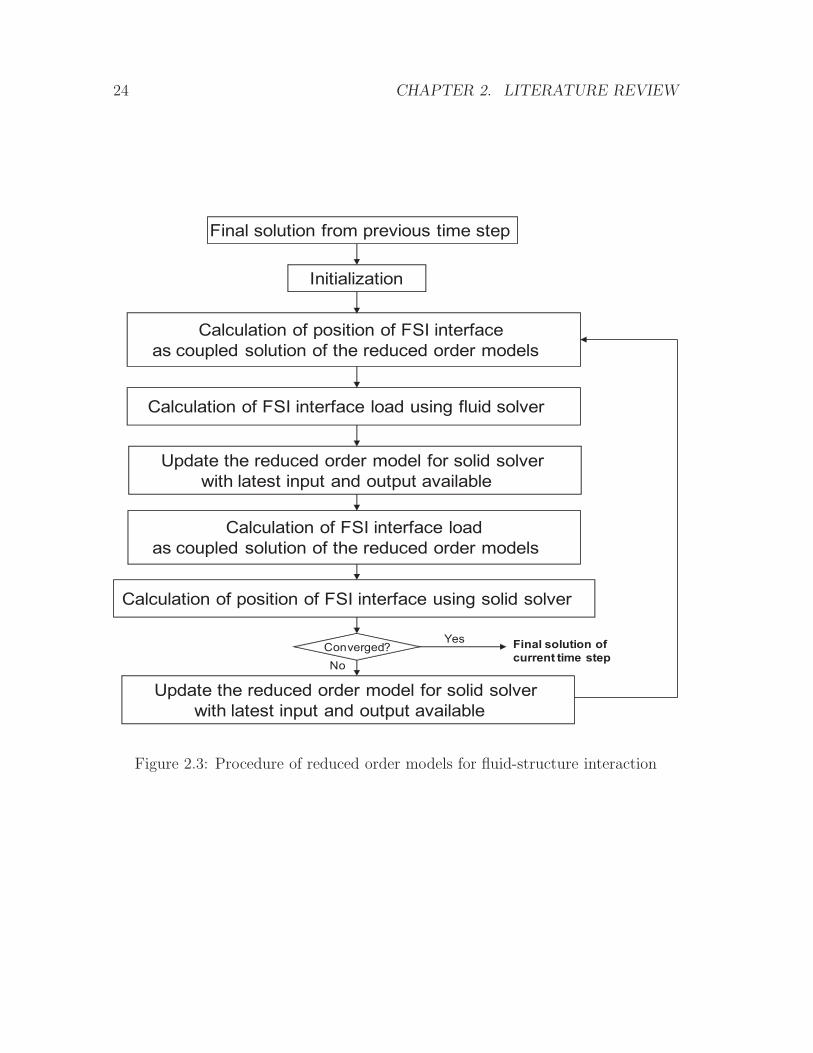
2.4.2 Reduced order models
The reduced order model was used in FSI simulation by numerous researchers such
as (Hall et al., 2000; Dowell and Hall, 2001; Willcox and Peraire, 2002) in order
to handle added-mass instability problem. By using this model, fluid solutions are
calculated with predefined deformation of domain boundary, which is used as FSI
interface. This is conducted to collect information about the response of flow field,
which corresponds to the prescribed deformation of the FSI interface. The reduced
order model is then constructed using this data. The reduced order model and solid
solver are then used to calculate for FSI solution. In 2007, Vierendeels et al. (2007)
introduced a similar method to improve the efficiency of partitioned approach FSI.
In this model, both fluid and solid solver are utilized to generate solution for fluid
and solid domain respectively. The reduced order model is used as a middleware
which help stabilize the coupling between fluid and solid solvers. The main task of
this middleware is to approximate the Jacobian of fluid and solid solver by using
least-squares models. The information used for constructing this models are the
solid and fluid solution that are obtained in the previous iterations. Recently, Wang
and Yan (2010) also presented sensitivity analysis and verificaton of the reduced
order model by comparing numerical results by using the reduced order model and
a physical experiment. Without detailed information of this reduced order model,
the procedure can be summarized as shown by Figure 2.3 according to Degroote
et al. (2008).
2.4.3 Artificial compressibility
Artificial compressibility was first used in numerical simulation by Chorin (1967)
to relax coupling of continuity and momentum equations for solving incompressible
flow. It is a numerical manipulation for improving coupling between momentum
and continuity equation, which leads to the improvement of convergence rate of
24 CHAPTER 2. LITERATURE REVIEW
Final solution from previous time step
Initialization
Calculation of position of FSI interface
as coupled solution of the reduced order models
Calculation of FSI interface load
as coupled solution of the reduced order models
Calculation of FSI interface load using fluid solver
Update the reduced order model for solid solver
with latest input and output available
Calculation of position of FSI interface using solid solver
Update the reduced order model for solid solver
with latest input and output available
No
YesConverged? Final solution of
current time step
Figure 2.3: Procedure of reduced order models for fluid-structure interaction
2.5. METHODS FOR COMPUTATONAL MESH IN FSI 25
solution (Rogers et al., 1987; Carter and Baker, 1991; Peyret, 1976; Merkle and
Athavale, 1987). In 2001, this technique is applied to stabilized coupling between
fluid and solid equations (Raback et al., 2001). Recently, the so-called “Interface
artificial compressibility” was introduced by Degroote et al. (2009), where the arti-
ficial term is applied to interface elements. It has been proved by the author that
this technique can stabilize the severe instability of FSI coupling. The main idea
of the method lies in the introduction of artificial compressibility into equations of
motion in the way that the final results are not affected by this additional term. The
interface artificial compressibility is modeled as a source term in continuity equation
in order to account for position of interface implicitly.
2.5 Methods for computatonal mesh in FSI
Meshing is an important issue in FSI as it has to deal with the movement of the
interface especially in problems with large deformation. For the completeness of
this review, existing methods for calculating computational mesh for fluid-structure
interaction simulation are discussed in this section.
2.5.1 Fixed grid algorithm
Fixed grid algorithms for fluid domain in FSI are very attractive and have been
widely used in recent years (Hieber and Koumoutsakos, 2008; Wall, Gerstenberger,
Gamnitzer, Forster and Ramm, 2006; Gerstenberger and Wall, 2008; Peskin, 2002).
This is mainly because fixed grid algorithms eliminate the need for using remeshing,
mesh smoothing for handling large deformation, which is common in FSI. More-
over, there is no need for the calulation of mesh velocity since governing equation
is described in Eulerian frame of reference when using fixed grid algorithms. Its
advantages mentioned above can lead to a significant reduction in computational
cost. However, the main drawback of fixed grid algorithm is the low resolution of
result near the boundary of interaction between fluid and solid. The methods used
for treating this disadvantage of fixed grid algorithm are:
26 CHAPTER 2. LITERATURE REVIEW
• Immerse boundary method;
• Chimera method;
• Extended Finite Element Method coupled with Lagrange Multiplier (XFEM/LM).
Immersed boundary method
A fully fixed grid schemes such as the immersed boundary method (IBM) em-
ploys a direct structural boundary representation over an Eulerian fluid mesh with-
out recourse to remeshing (Hieber and Koumoutsakos, 2008; Peskin, 2002; Zhang
et al., 2004). The structure is treated as some form of fictitious fluid domain which
deforms according to the surrounding fluid velocity. This is implemented by inter-
polating the velocity of surrounding fluid nodes to the structural nodes (Wall, Ger-
stenberger, Gamnitzer, Forster and Ramm, 2006). Meanwhile, the structural effects
on the fluid is realized by spreading the Lagrangian elastic forces of the structure
in the form of additional body forces to neighbouring fluid nodes. Both these inter-
actions between Lagrangian and Eulerian variables are implemented by employing
interesting properties of the Dirac delta functions. In order to numerically imple-
ment the scheme, smooth functions to mimic the properties of dirac delta functions
are necessary, leading to the concept of bounded support to efficiently define the
extent of influence for each nodal variable.
The spreading of the structural forcing function indirectly smears the boundary
of the fluid-structure interface. This limits spatial accuracy of the IBM to its mesh-
width and its inability to accurately capture sharp interfaces. Furthermore, without
structural position a priori, accurate resolution of boundary layers is also a concern.
An immersed interface method and adaptive mesh refinement schemes have been
proposed to overcome these drawbacks (Peskin, 2002).
Chimera method
Wall, Gerstenberger, Gamnitzer, Forster and Ramm (2006) used the Chimera
method, which was introduced by Steger et al. (1983), for solving problems in FSI.
2.5. METHODS FOR COMPUTATONAL MESH IN FSI 27
Numerous studies have been conducted to improve this method (Brezzi et al., 2001;
Glowinski et al., 2005; Peterson, 1999). Fundamentally, the fluid domain is decom-
posed to a background Eulerian fluid domain and a ALE fluid subdomain, which
overlapped each other. The background Eulerian fluid domain does not extend to
the structural boundary, while the ALE fluid subdomain is a deformable fluid sub-
domain that is attached to the solid domain at interface. This means the ALE fluid
subdomain follows the structural movement in order to a local resolution at inter-
face of interaction. Meanwhile, the information between the Eulerian and ALE fluid
subdomains are driven by applying Dirichlet and Neumann boundary conditions
through interpolation and iteration process.
Extended finite element method coupled with lagrange multiplier
Another fully fixed grid approach include an extended Finite Element Method cou-
pled with Lagrange Multiplier (XFEM/LM) technique proposed by Wall, Gersten-
berger, Gamnitzer, Forster and Ramm (2006) and Gerstenberger and Wall (2008).
Employing an enrichment jump shape function to capture variable discontinuity,
XFEM enables separation of the Eulerian fluid domain to its physical and non-
physical subdomains across an interface, allowing more accurate treatment of the
interface. The interface grids are free to move and can be coupled to another moving
domain. The compatibility between the generally non-matching 3-field grids (physi-
cal fluid domain, moving and interface domains) are achieved by applying a lagrange
multiplier technique. The scheme can be enhanced by introducing adaptive grid re-
finement, driven by either heuristic or error indicators, to better capture flow near
the interface. However, to efficiently capture boundary layers, the moving domain
could also be set to consist of an ALE fluid subdomain coupled to the Lagrangian
structural domain. Unlike Chimera schemes, there is no overlap of fluid subdomains
and hence open to both partitioned and monolithic solving.
28 CHAPTER 2. LITERATURE REVIEW
2.5.2 Moving mesh
In fluid-structure interaction, moving mesh is often used to handle deformation
of FSI interface. It is important to note that the movement of deforming grid
should satisfy “Geometric conservation law” (Lesoinne and Farhat, 1996; Koobus
and Farhat, 1999; Guillard and Farhat, 2000; C. Farhat and Grandmont, 2001). The
principle statement of this law is that the volume which is swept by interface must be
equal to the change in volume of the element that experience the sweep of interface.
This law mainly influences the way, which mesh velocity in moving grid domain is
calculated. The mesh velocity is usually calculated using first order time integration
scheme, which does not always satisfy this law (Donea et al., 2004). Even though the
geometric conservation law is believed to be the drive for solution modelled in ALE
frame of reference (C. Farhat and Grandmont, 2001) but it has been controversial to
determine if this law is essential to calculating moving mesh (Guillard and Farhat,
2000).
Up to date, there are several methods of governing moving mesh. Spring analogy
method was introduced by Batina (1989) which was generally used for unstructured
meshes only before it was improved by Robinson et al. (1991) for dealing with
structured meshes. Despite its ability to handle considerably large deformation, it
is often considered computationaly expensive when used for large mesh sizes. In
this method, the movement of the nodes are determined by solving an elliptic grid
generator iteratively. Later, a simple algebraic shearing technique was proposed
by Schuster et al. (1990) which recalculates movement of nodes along nodes lines
that are normal to FSI interface. This technique is quite limited as it cannot deal
with complex geometries and large deformation. Eriksson (1982) introduced a three
stage transfinite interpolation (TFI) method which can only be used for single block
mesh before it was improved in the work done by Hartwich and Agrawal (1997). The
TFI method was combined with spring analogy method such that the movement of
the interface nodes is done by spring analogy while that of interior nodes is done by
TFI.
2.6. SUMMARY AND CONCLUDING REMARKS 29
2.5.3 Automatic remeshing
In some FSI problems, the automatic remeshing of compuational domain is required
due to excessively large deformation, which cannot be handled by using mesh moving
methods such as the spring analogy method. However, it is common that automatic
remeshing is used in conjunction with a mesh movement method. By doing this,
computational cost for remeshing can be minimized because remeshing will only be
executed when quality of computational elements become lower than an acceptable
level. The computational cost for remeshing can be expensive because remeshing
generally requires generation of totally new mesh and then mapping the solution
from the previous mesh onto it. Skewness and aspect ratio can be used as initiators of
the remeshing process (ANSYS Inc. 2009. ANSYS CFX-Solver Theory Guide, n.d.).
2.6 Summary and concluding remarks
In this chapter, some important terminologies and techniques used in the field of
FSI are discussed. From the best of the author’s knowledge, The implementation
of most of the existing techniques requires intensive modifications or even cannot
be done at all in some commercial software. This leaves us with two most obvious
choices, which are under-relaxation technique and artificial compressibility, for deal-
ing the instability. Firstly, under-relaxation technique is commonly used in most FSI
software but its efficiency is not good for solving most engineering applications. Sec-
ondly, artificial compressiblity is a quite simple technique to be applied in any CFD
codes. Therefore, these two techniques are choosen for this work for performance
comparison both theoretically and numerically in later chapters.

30 CHAPTER 2. LITERATURE REVIEW
Chapter 3
Methodology
In this chapter, we will discuss our strategy and method to obtain numerical results.
Governing equations for fluid and structural mechanics is discussed. Discritization
for the governing equations gives the underlining method of solving these governing
equations. The procedure for calculating the fluid strucuture interaction is provided.
We also discuss the construction and set up for meshing.
3.1 Governing equations
3.1.1 Fluid governing equation
Fluid governing equations consist of the following equations:
• Continuity equation: conservation of mass;
• Momentum equaton: conservation of momentum;
• Energy equation: conservation of energy.
Continuity equation
The continuity equation is based on the idea that any mass in the system has to be
conserved. In other words, matter can neither be created or destroyed. This means
31
32 CHAPTER 3. METHODOLOGY
that the rate of change of mass within the control volume is equivalent to the mass
flux crossing the surface S of volume V . After some mathematical manipulations,
a general form of continuity equation in the Eulerian frame can be written as
∂ρ
∂t+∇ · (ρv) = 0, (3.1)
where ρ is density, t is time and v is velocity.
The continuity equation is reformulated in ALE reference frame. It can be writ-
ten as
∂ρ
∂t+∇ · (ρ(v − vc)) = 0, (3.2)
∂ρ
∂t+∇ · ρ(v − vc) = 0, (3.3)
where vc is grid velocity.
Momentum equation
The momentum equation can be formulated based on a physical principle that mo-
mentum in the system has to be conserved. A general form of momentum equation
in the Eulerian frame can be written as
ρ∂v
∂t+ ρ (v · ∇)v = ∇ · (ρΥ∇v), (3.4)
where Υ is diffusivity.
The momentum equation is reformulated in the ALE reference frame. It can be
written as
ρ∂v
∂t+ ρ ([v − vc] · ∇)v = ∇ · (ρΥ∇v). (3.5)
3.2. DISCRETIZATION FOR GOVERNING EQUATIONS 33
Energy equation
The energy equation can be formulated based on a physical principle that energy
in the system has to be conserved. A general form of energy equation in Eulerian
frame can be written as
ρ∂E
∂t+ ρ (v · ∇)E = ∇ · (ρΥ∇E), (3.6)
where E is energy.
The energy equation is reformulated in the ALE reference frame. It can be
written as
ρ∂E
∂t+ ρ ([v − vc] · ∇)E = ∇ · (ρΥ∇E). (3.7)
3.1.2 Solid governing equation
The governing equation for solid domain is formulated in the Largrangian reference
frame. It can be written as
Md+Cd+Kd = F, (3.8)
where d is displacement, M is mass, C is damping, K is stiffness and F is force.
3.2 Discretization for governing equations
In this section, discretization schemes used in calculation of both fluid and solid
solution will be discussed.
3.2.1 Discretization for fluid governing equations
We start with a generic form of fluid governing equation in the ALE frame of refer-
ence which is written as
34 CHAPTER 3. METHODOLOGY
∂ρφ
∂t︸︷︷︸Temporal term
+O · (ρ [v − vc]φ)︸ ︷︷ ︸Convection term
−O · (ρΥφOφ)︸ ︷︷ ︸Disffusion term
= Sφ (φ)︸ ︷︷ ︸Source term
, (3.9)
where φ is a transport variable, Υφ is diffusivity, Sφ is a source term.
In finite volume method, it is required that the governing equation is satisfied
over control volume VP around point P. Therefore, it can be rewritten in the
intergral form as
∫ t+4t
t
∂
∂t
∫
VP
ρφdVP
︸ ︷︷ ︸Temporal term
+
∫
VP
O · (ρ [v − vc]φdVP
︸ ︷︷ ︸Convection term
−∫
VP
O · (ρΥφOφ) dVP
︸ ︷︷ ︸Disffusion term
=
∫ t+4t
t
∫
VP
Sφ (φ) dVP
︸ ︷︷ ︸Source term
.(3.10)
The following discretization schemes used for each term in transport equation of
fluid are presented.
Temporal term
• First order backward Euler scheme. By using this scheme, the discretized
temporal term can be written as
∂
∂t
∫
VP
ρφdVP = VP
(ρn+1φn+1 − ρnφn
4t
), (3.11)
where superscript n+1 and n denote time level n+1 and n respec-
tively.
• Second order backward Euler scheme. By using this scheme, the dis-
cretized temporal term can be written as
3.2. DISCRETIZATION FOR GOVERNING EQUATIONS 35
∂
∂t
∫
VP
ρφdVP = VP
(3 (ρn+1φn+1)− 4 (ρnφn) + (ρn−1φn−1)
24t
). (3.12)
Convection term
The convection term can be put into discretized form by using the Gauss’s theorem
as
∫
VP
O · (ρ [v − vc]φ) dVP =∑
fc
Sc (ρ [v − vc]φ)fc
=∑
fc
Sc (ρ [v − vc])fc φfc
=∑
fc
Fcφfc. (3.13)
Note that Sc and Fc are the outward-pointing face area vector and mass flux
through element face. The convection term can be calculated if the flux value
on surface of element is known by simple interpolation. The subscript fc denotes
the element face. Now, variable φfc is the only unknown left before calculation of
convection term can be achieved. Therefore, the main purpose of the convection
differencing scheme is to evaluate φfc on faces of computational elements by using
the value of φ at the center of elements. The followings are convection differencing
schemes available in CFX.
• First order upwind differencing scheme.
φfc =
{φfc = φP if Fc ≥ 0
φfc = φP if Fc < 0(3.14)
• Central differencing scheme
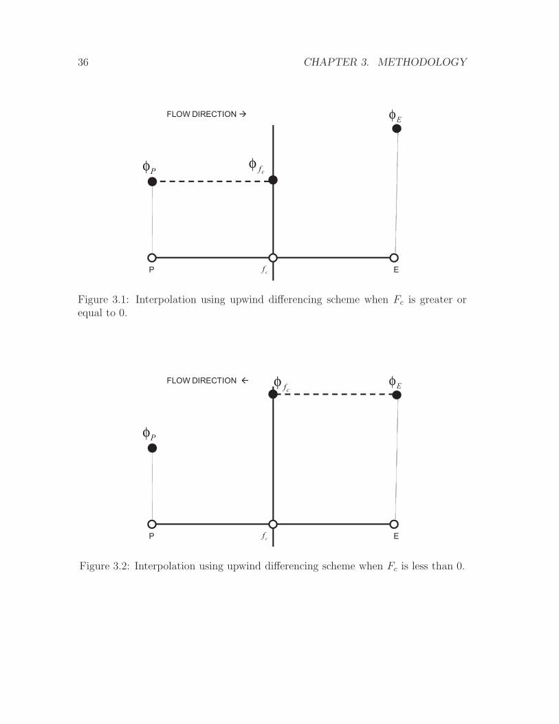
36 CHAPTER 3. METHODOLOGY
P E
Pφcf
φ
Eφ
cf
FLOW DIRECTION à
Figure 3.1: Interpolation using upwind differencing scheme when Fc is greater orequal to 0.
P E
Pφ
cfφ Eφ
cf
FLOW DIRECTION ß
Figure 3.2: Interpolation using upwind differencing scheme when Fc is less than 0.
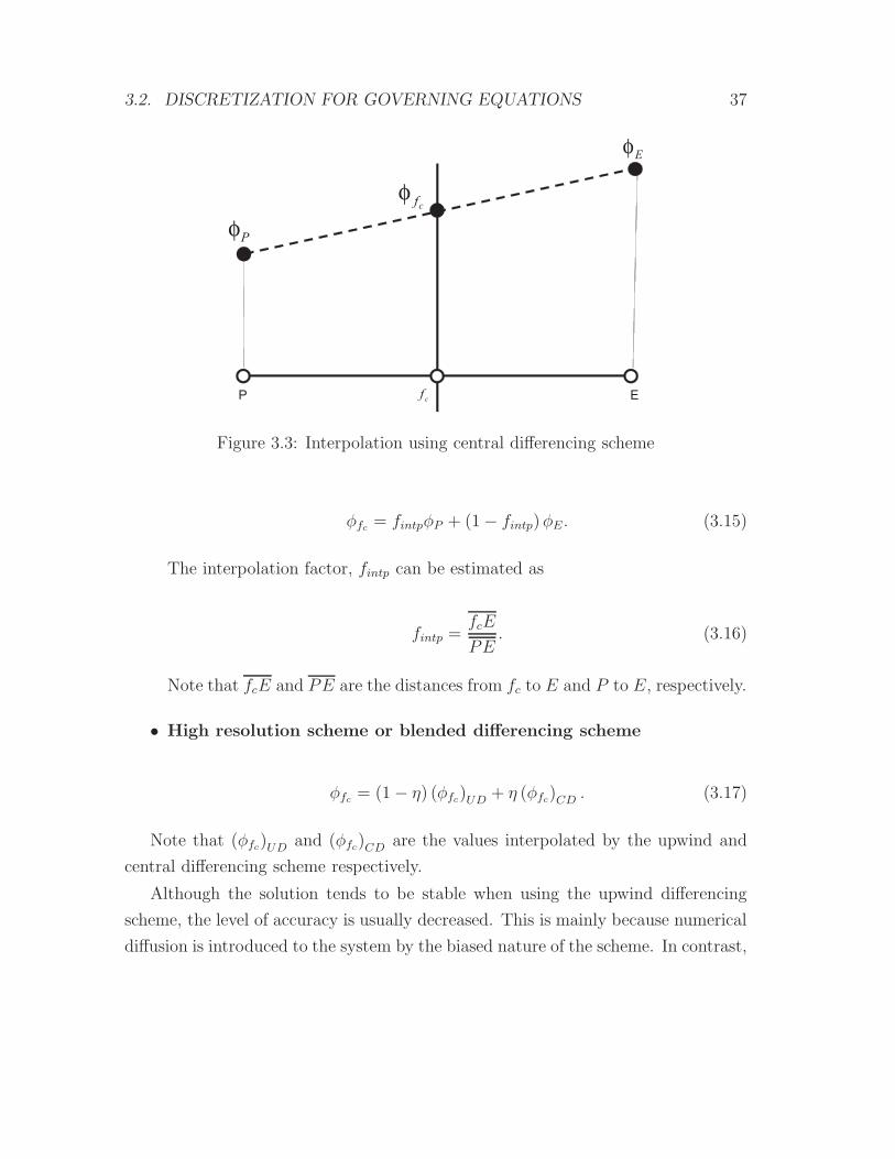
3.2. DISCRETIZATION FOR GOVERNING EQUATIONS 37
P E
Pφ
cfφ
Eφ
cf
Figure 3.3: Interpolation using central differencing scheme
φfc = fintpφP + (1− fintp)φE . (3.15)
The interpolation factor, fintp can be estimated as
fintp =fcE
PE. (3.16)
Note that fcE and PE are the distances from fc to E and P to E, respectively.
• High resolution scheme or blended differencing scheme
φfc = (1− η) (φfc)UD+ η (φfc)CD
. (3.17)
Note that (φfc)UDand (φfc)CD
are the values interpolated by the upwind and
central differencing scheme respectively.
Although the solution tends to be stable when using the upwind differencing
scheme, the level of accuracy is usually decreased. This is mainly because numerical
diffusion is introduced to the system by the biased nature of the scheme. In contrast,
38 CHAPTER 3. METHODOLOGY
the central differencing scheme is less biased in nature, which provides a second order
of accuracy at the expense of stability. Therefore, the use of blended differencing
scheme is introduced to preserve both stability and accuracy of solution. It is a
combination of upwind and central differencing scheme, where the contribution of
upwind and central differencing scheme is determined by η. The Blended differencing
scheme reduces to upwind differencing scheme when η is chosen to be zero. It also
reduces to central differencing scheme when η is chosen to be unity.
Diffusion term
The diffusion term can be put into discretized form by using the Guass’s theorem
as
∫
VP
O · (ρΥφOφ) dVP =∑
fc
Sc (ρΥφOφ)fc
=∑
fc
(ρΥφ)fc Sc (Oφ)fc . (3.18)
To be able to calculate diffusion term, the most important task is to correctly
estimate (Oφ)fc . Here,
(Oφ)fc =
(∂φ
∂x
)
fc
+
(∂φ
∂y
)
fc
+
(∂φ
∂z
)
fc
, (3.19)
(∂φ
∂x
)
fc
=∑
nd
(∂Nnd
∂x
)
fc
φnd,
(∂φ
∂y
)
fc
=∑
nd
(∂Nnd
∂y
)
fc
φnd.
(∂φ
∂z
)
fc
=∑
nd
(∂Nnd
∂z
)
fc
φnd. (3.20)
3.2. DISCRETIZATION FOR GOVERNING EQUATIONS 39
Note that formula of shape function Nnd depends on shape of computational
element being considered during calculation (ANSYS Inc. 2009. ANSYS CFX-
Solver Theory Guide, n.d.).
Source term
A simple linearlization is applied to discretize source term in fluid transport equa-
tion. As suggested by (Patankar, 1980), the discretized source term can be written
as
∫
VP
Sφ (φ) dVP = SuVP + SPVPφP. (3.21)
Interface fluid acceleration
The backward Euler is used for the discretization of fluid acceleration. The first
order backward Euler can be written as
vn+1 − vn
4t= vn+1, (3.22)
while the second order backward Euler can be put as
vn+1 − vn
4t=
1
3
vn − vn−1
4t+
2
3vn+1. (3.23)
In this paper, only the zeroth order structural predictor is used in order to
estimate the fluid deformation corresponding to structural displacement of previous
time step dn.
The structural predictor can be written as
dn+1Γ,P = dnΓ. (3.24)
40 CHAPTER 3. METHODOLOGY
3.2.2 Discretization for solid governing equation
The nonlinear version of the generalized-α time integration scheme, which was in-
troduced by (Chung and Hulbert, 1993), can be used for discretization of solid
governing equation as mentioned by (Bathe, 1996). The method assumes that
dn+1 = dn +[(1− δ) dn + δdn+1
]4t, (3.25)
dn+1 = dn + dn4t+
[(1
2− α
)dn + αdn+1
]4t2. (3.26)
According to (ANSYS Inc. 2009. ANSYS CFX-Solver Theory Guide, n.d.),
after some mathematical manipulations, equations (3.25) and (3.26) can be recast
in equations (3.27) and (3.28) respectively as
dn+1 = dn +4t (1− δ) dn +4tδdn+1, (3.27)
dn+1 =1
α4t2(dn+1 + dn
)− 1
α4tdn −
(1
2α− 1
)dn. (3.28)
The value of structural displacement, velocity and acceleration is interpolated
between time level as
dn+1,α = (1− αm) dn+1 + αmd
n, (3.29)
dn+1,α = (1− αf ) dn+1 + αf d
n, (3.30)
dn+1,α = (1− αf ) dn+1 + αfd
n. (3.31)
By using the equations for dn+1 and dn+1, the discretized solid governing equation
can be written as
3.2. DISCRETIZATION FOR GOVERNING EQUATIONS 41
(a0M+ a1C+ (1− αf )K) dn+1 = (1− αf )Fn+1ext + αfF
next − αfF
nint
+M(a0d
n + a2dn + a3d
n)
+C(a1d
n + a4dn + a5d
n). (3.32)
The coefficients required in above equations are provided as follows.
a0 =1− αm
α4t2, a1 =
δ (1− αf)
α4t, a2 =
1− αm
α4t, a3 =
1− αm
2α− 1 ,
a4 =δ (1− αm)
α− 1 , a5 = 4t (1− αm)
(δ
2α− 1
)(3.33)
In order to maintain unconditional stability and second order accuracy of time
integration, the following criteria must be satisfied (ANSYS Inc. 2009. ANSYS
CFX-Solver Theory Guide, n.d.).
δ ≥ 1
2, α ≥ 1
2δ , δ =
1
2− αm + αf , αm ≥ αf ≥ 1
2. (3.34)
The studies by (Wood et al., 1981) suggests that these parameters can be written
in terms of amplitude decay factor γ as
α =1
4(1 + γ)2 , δ =
1
2+ γ , αf = 0 , αm = −γ. (3.35)
When minimum numerical damping is applied, the value of α, δ, αm and αf are
set to be 14, 1
2, 0, 0 respectively. These values represent time integration which has
zero numerical damping. This can be achieved by setting γ = 0. The equations for
dn+1 and dn+1 can be put as
dn+1 = dn +1
24tdn +
1
24tdn+1, (3.36)
42 CHAPTER 3. METHODOLOGY
dn+1 =4
4t2
[dn+1 + dn −4tdn − 4t2
4dn]. (3.37)
After some mathematical manipulation, the structural acceleration can be writ-
ten in terms of deformation at different time levels as
dn+1,α ≈ 1
4t2(4dn+1 − 16dn + 32dn−1 − 20dn−2
)− 12
4tdn−2 − dn−2. (3.38)
This time integration scheme cannot be put in terms of displacement only and it
has the fully recursive characteristics which means that the calculation of time step
n+ 1 utilizes information of all previous time steps down to the intial step.
When maximum numerical damping is applied, the values of α, δ, αm and αf are
set to be 1, 32, -1 and 0 respectively. This can be alternatively achieved by setting
γ = 1. Therefore, equations for dn+1 and dn+1 can be written as
dn+1 = dn +1
24tdn +
3
24tdn+1, (3.39)
dn+1 =1
4t2
[dn+1 + dn −4tdn − 4t2
2dn]. (3.40)
Subsequently, this leads to
dn+1,α =1
4t2(2dn+1 − 5dn + 4dn−1 − dn−2
). (3.41)
3.3 Fundamental conditions for FSI coupling
The conditions required when solving FSI are kinematic and dynamic ones, which is
suggested by the work by Wang and Yan (2010). The kinematic condition ensures
the compatibility of displacement across FSI interface. It can be written as
dfΓ = dsΓ, (3.42)
3.4. IMPLEMENTATION OF ARTIFICIAL COMPRESSIBILITY 43
where d is displacement, dsΓ and dfΓ are the displacement of the solid and fluid
interface, respectively. This condition leads to a relationship between fluid velocity
vΓ and rate of change of displacement, which can be written as
n · vΓ = n · dsΓ, (3.43)
where n is normal vector on the interface.
If no-slip condition is used on the fluid side of the FSI interface. The dynamic
condition ensures the compatibility of traction across FSI interface. It can be written
as
n · σsΓ = n · σf
Γ, (3.44)
where σΓ represents stress on the interface.
These two conditions are normally utilized in FSI codes, which adopts the parti-
tioned approach. By following the kinematic condition, fluid nodes on FSI interface
are updated according to their corresponding solid nodes. By following the dynamic
condtion, the equilibrium of stress on FSI interface is ensured and the fluid pressure
is integrated into fluid force which is used when applying to solid nodes along inter-
face. A simple diagram can illustrate that these two conditions force the transfer of
interface loads across FSI interface as shown in Figure 3.4
3.4 Implementation of artificial compressibility
In this section, the implementation of artificial compressibility is discussed. In this
thesis, artificial compressibility is applied to solution system of fluid-structure inter-
action of working fluid. The density of fluid is generally written as follows:
If working fluid is modelled as incompressible flow, then
ρ = ρ0 +Artificial compressibility. (3.45)
If working fluid is modelled as compressible flow, then
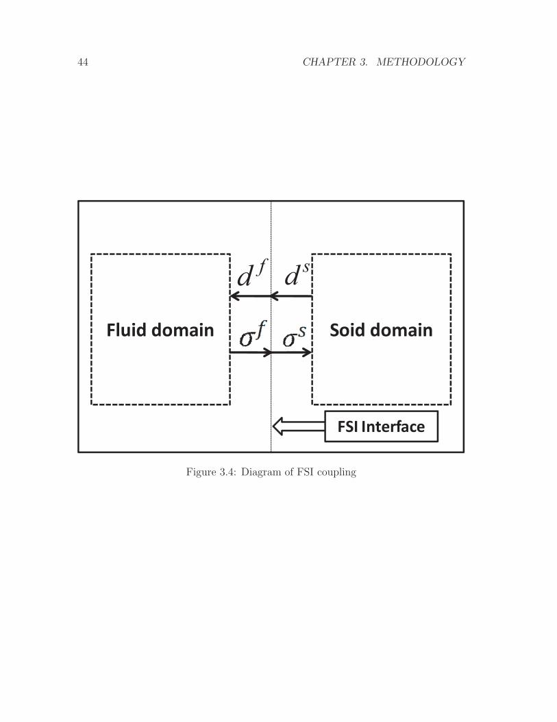
44 CHAPTER 3. METHODOLOGY
Fluid domain Soid domain
FSI Interface
sdfd
Figure 3.4: Diagram of FSI coupling
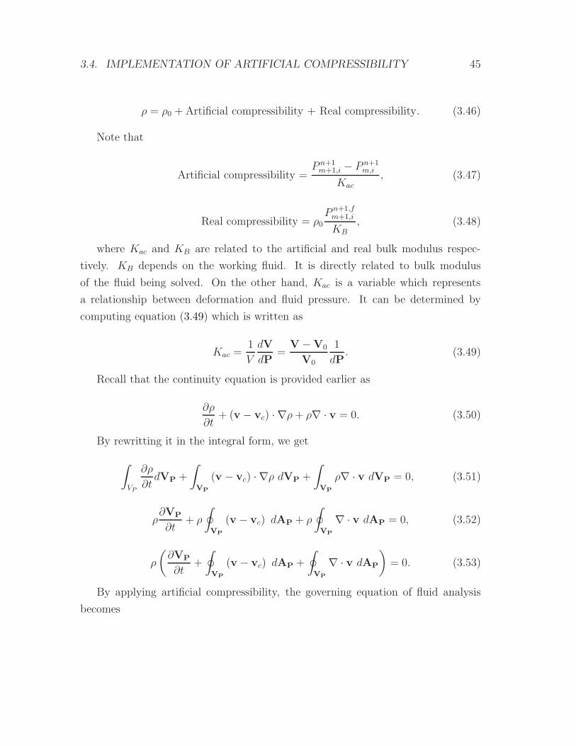
3.4. IMPLEMENTATION OF ARTIFICIAL COMPRESSIBILITY 45
ρ = ρ0 +Artificial compressibility + Real compressibility. (3.46)
Note that
Artificial compressibility =P n+1m+1,i − P n+1
m,i
Kac
, (3.47)
Real compressibility = ρ0P n+1,fm+1,i
KB
, (3.48)
where Kac and KB are related to the artificial and real bulk modulus respec-
tively. KB depends on the working fluid. It is directly related to bulk modulus
of the fluid being solved. On the other hand, Kac is a variable which represents
a relationship between deformation and fluid pressure. It can be determined by
computing equation (3.49) which is written as
Kac =1
V
dV
dP=
V −V0
V0
1
dP. (3.49)
Recall that the continuity equation is provided earlier as
∂ρ
∂t+ (v− vc) · ∇ρ+ ρ∇ · v = 0. (3.50)
By rewritting it in the integral form, we get
∫
VP
∂ρ
∂tdVP +
∫
VP
(v − vc) · ∇ρ dVP +
∫
VP
ρ∇ · v dVP = 0, (3.51)
ρ∂VP
∂t+ ρ
∮
VP
(v − vc) dAP + ρ
∮
VP
∇ · v dAP = 0, (3.52)
ρ
(∂VP
∂t+
∮
VP
(v − vc) dAP +
∮
VP
∇ · v dAP
)= 0. (3.53)
By applying artificial compressibility, the governing equation of fluid analysis
becomes
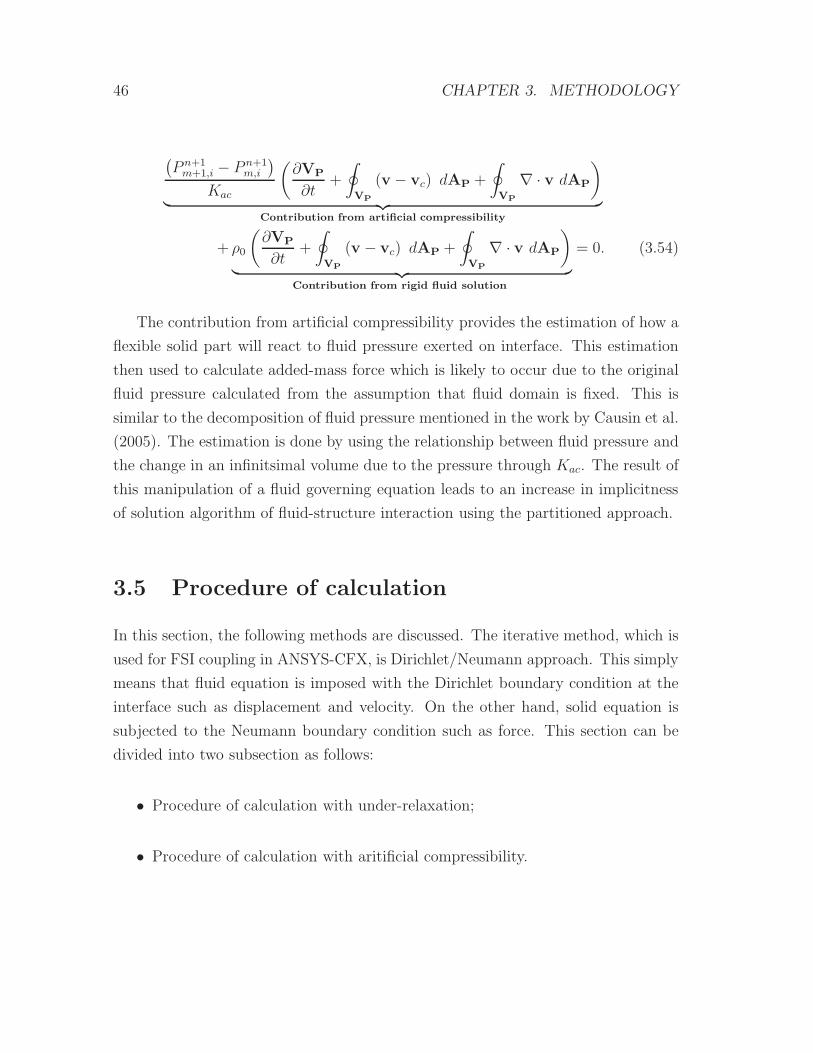
46 CHAPTER 3. METHODOLOGY
(P n+1m+1,i − P n+1
m,i
)
Kac
(∂VP
∂t+
∮
VP
(v − vc) dAP +
∮
VP
∇ · v dAP
)
︸ ︷︷ ︸Contribution from artificial compressibility
+ ρ0
(∂VP
∂t+
∮
VP
(v − vc) dAP +
∮
VP
∇ · v dAP
)
︸ ︷︷ ︸Contribution from rigid fluid solution
= 0. (3.54)
The contribution from artificial compressibility provides the estimation of how a
flexible solid part will react to fluid pressure exerted on interface. This estimation
then used to calculate added-mass force which is likely to occur due to the original
fluid pressure calculated from the assumption that fluid domain is fixed. This is
similar to the decomposition of fluid pressure mentioned in the work by Causin et al.
(2005). The estimation is done by using the relationship between fluid pressure and
the change in an infinitsimal volume due to the pressure through Kac. The result of
this manipulation of a fluid governing equation leads to an increase in implicitness
of solution algorithm of fluid-structure interaction using the partitioned approach.
3.5 Procedure of calculation
In this section, the following methods are discussed. The iterative method, which is
used for FSI coupling in ANSYS-CFX, is Dirichlet/Neumann approach. This simply
means that fluid equation is imposed with the Dirichlet boundary condition at the
interface such as displacement and velocity. On the other hand, solid equation is
subjected to the Neumann boundary condition such as force. This section can be
divided into two subsection as follows:
• Procedure of calculation with under-relaxation;
• Procedure of calculation with aritificial compressibility.
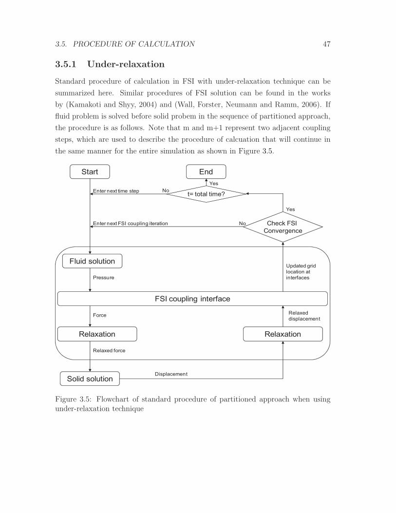
3.5. PROCEDURE OF CALCULATION 47
3.5.1 Under-relaxation
Standard procedure of calculation in FSI with under-relaxation technique can be
summarized here. Similar procedures of FSI solution can be found in the works
by (Kamakoti and Shyy, 2004) and (Wall, Forster, Neumann and Ramm, 2006). If
fluid problem is solved before solid probem in the sequence of partitioned approach,
the procedure is as follows. Note that m and m+1 represent two adjacent coupling
steps, which are used to describe the procedure of calcuation that will continue in
the same manner for the entire simulation as shown in Figure 3.5.
Start
Fluid solution
FSI coupling interface
Pressure
Force
Solid solution
Relaxation
Displacement
Relaxation
Relaxed force
Relaxed
displacement
Check FSI
Convergence
End
t= total time?
No
Yes
Enter next FSI coupling iteration
Yes
NoEnter next time step
Updated grid
location at
interfaces
Figure 3.5: Flowchart of standard procedure of partitioned approach when usingunder-relaxation technique
48 CHAPTER 3. METHODOLOGY
1. Compute initial configuration of fluid domain by using information passed
from previous time step, dn in case of the first coupling step of time step level
n+1, otherwise information passed from previous coupling iteration, dn+1m will
be used instead. That is
dn+1m+1 =
dn if m = 0
dn+1m if m 6= 0,
(3.55)
where denotesthatthedisplacementisonlyanestimation.
2. Solve fluid field using a fluid solver to get
P n+1m+1 = F
(dn+1m+1
), (3.56)
where P represents fluid pressure, F represents fluid calculation.
3. Transfer fluid load obtained to solid solver and estimate corresponding load to be
applied in solid solver. That is
P n+1m+1 = ω
(P n+1m+1
), (3.57)
where ω is an applied under-relaxation factor.
4. Solve solid governing equation to get
dn+1m+1 = S
(P n+1m+1
), (3.58)
where S represents solid calculation.
5. Estimate deformation of fluid domain, which is corresponding to solid solution ob-
tained from previous step. That is
dn+1m+1 = (1− ω) dn+1
m+1 + ωdn+1m . (3.59)
3.5. PROCEDURE OF CALCULATION 49
Note that dn+1m+1 is not the final solid solution but only an estimation for fluid calcu-
lation at coupling level m+ 1.
6. Check for convergence. The solution is converged if the following conditions is
applied. Here,
rn+1,s < ε0, rn+1,s = dn+1m+1 − dn+1
m , (3.60)
rn+1,f < ε0, rn+1,f = P n+1m+1 − P n+1
m , (3.61)
where r is calculated residual, ε0 is a tolerance used for determining convergence of
solution. Note that superscripts s and f denotes solid and fluid respectively.
7. Proceed to next time step or finish simulation if convergence is reached. If con-
vergence is not reached, then continue the iteration process in a similar manner as
mentioned above.
If the under-relaxation factor and number of coupling iteration used for secondth
and sixth step are chosen to be 1, the FSI algorithm becomes explicit. Calculation
can be done in a similar manner if the solid problem is solved before fluid problem
in the sequence of partitioned approach.
3.5.2 Aritificial compressibility
Standard procedure of calculation in FSI with artificial compressibility can be pre-
sented here. For this technique, the artificial compressibility is applied to fluid
density as mentioned in the previous section. If the fluid problem is solved before
solid probem in the sequence of partitioned approach, the procedure is as follows.
Note that m and m + 1 represent two adjacent coupling steps which are used to
describe the procedure of calcuation that will continue in the same manner for the
entire simulation. The procedure of calculation above can be illustrated with a
simple diagram in Figure 3.6.
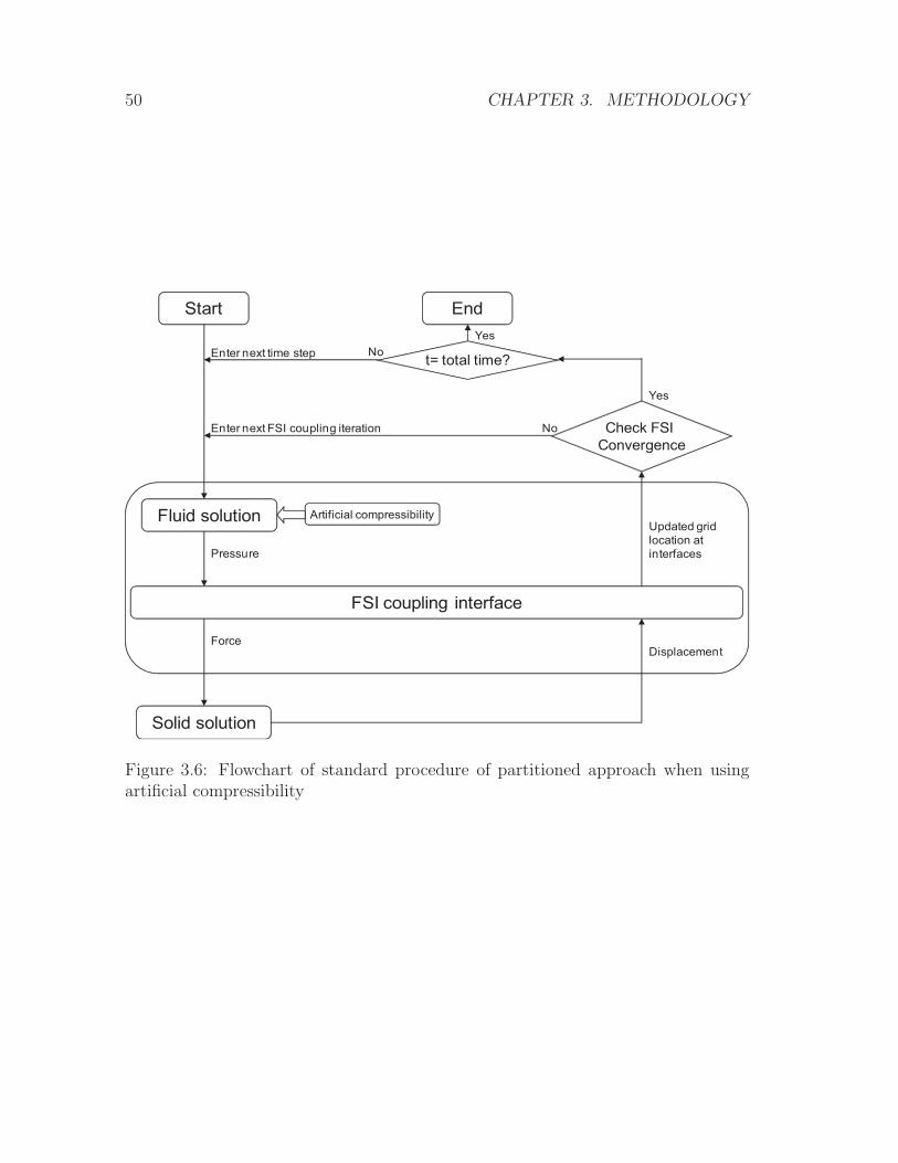
50 CHAPTER 3. METHODOLOGY
Start
Fluid solution
FSI coupling interface
Pressure
Force
Solid solution
Displacement
Check FSI
Convergence
End
t= total time?
No
Yes
Enter next FSI coupling iteration
Yes
NoEnter next time step
Updated grid
location at
interfaces
Artificial compressibility
Figure 3.6: Flowchart of standard procedure of partitioned approach when usingartificial compressibility
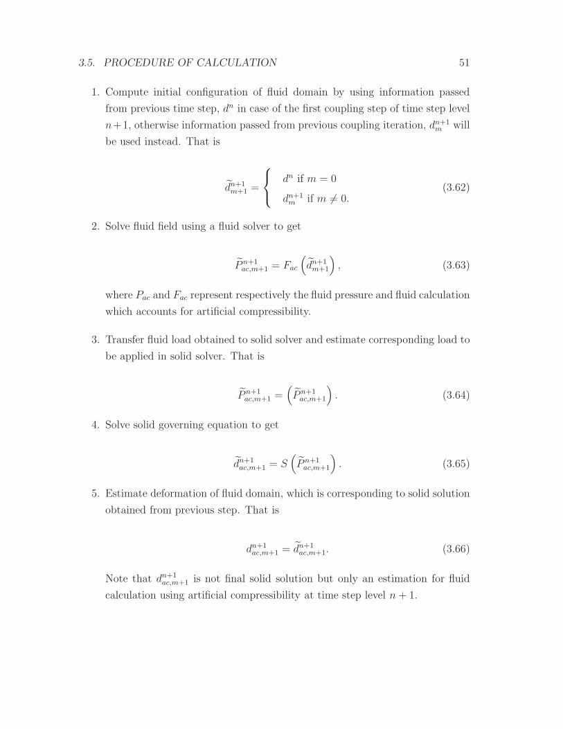
3.5. PROCEDURE OF CALCULATION 51
1. Compute initial configuration of fluid domain by using information passed
from previous time step, dn in case of the first coupling step of time step level
n+1, otherwise information passed from previous coupling iteration, dn+1m will
be used instead. That is
dn+1m+1 =
dn if m = 0
dn+1m if m 6= 0.
(3.62)
2. Solve fluid field using a fluid solver to get
P n+1ac,m+1 = Fac
(dn+1m+1
), (3.63)
where Pac and Fac represent respectively the fluid pressure and fluid calculation
which accounts for artificial compressibility.
3. Transfer fluid load obtained to solid solver and estimate corresponding load to
be applied in solid solver. That is
P n+1ac,m+1 =
(P n+1ac,m+1
). (3.64)
4. Solve solid governing equation to get
dn+1ac,m+1 = S
(P n+1ac,m+1
). (3.65)
5. Estimate deformation of fluid domain, which is corresponding to solid solution
obtained from previous step. That is
dn+1ac,m+1 = dn+1
ac,m+1. (3.66)
Note that dn+1ac,m+1 is not final solid solution but only an estimation for fluid
calculation using artificial compressibility at time step level n+ 1.
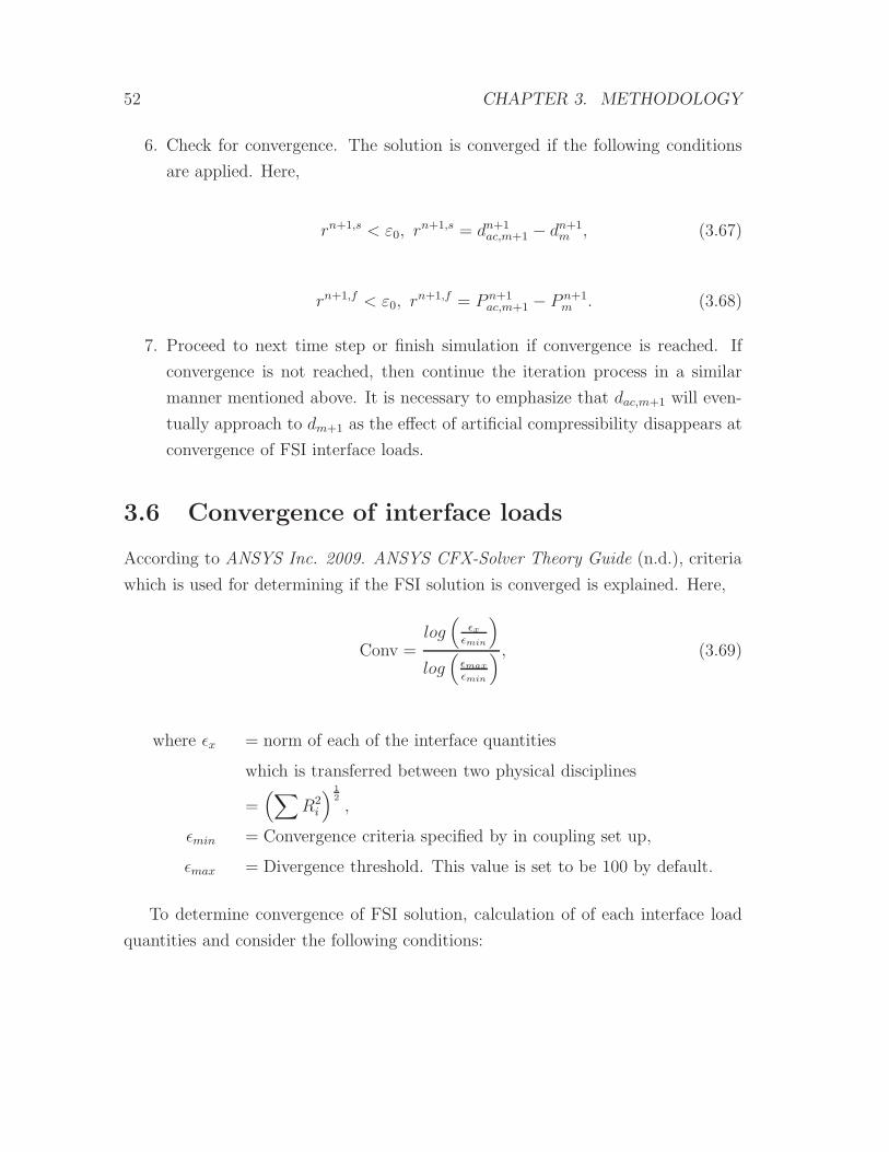
52 CHAPTER 3. METHODOLOGY
6. Check for convergence. The solution is converged if the following conditions
are applied. Here,
rn+1,s < ε0, rn+1,s = dn+1ac,m+1 − dn+1
m , (3.67)
rn+1,f < ε0, rn+1,f = P n+1ac,m+1 − P n+1
m . (3.68)
7. Proceed to next time step or finish simulation if convergence is reached. If
convergence is not reached, then continue the iteration process in a similar
manner mentioned above. It is necessary to emphasize that dac,m+1 will even-
tually approach to dm+1 as the effect of artificial compressibility disappears at
convergence of FSI interface loads.
3.6 Convergence of interface loads
According to ANSYS Inc. 2009. ANSYS CFX-Solver Theory Guide (n.d.), criteria
which is used for determining if the FSI solution is converged is explained. Here,
Conv =log(
εxεmin
)
log(
εmax
εmin
) , (3.69)
where εx = norm of each of the interface quantities
which is transferred between two physical disciplines
=(∑
R2i
) 1
2
,
εmin = Convergence criteria specified by in coupling set up,
εmax = Divergence threshold. This value is set to be 100 by default.
To determine convergence of FSI solution, calculation of of each interface load
quantities and consider the following conditions:
3.7. GENERAL PROCEDURE OF FSI SIMULATION SETUP 53
• If εx < εmin, then solution has converged;
• If εx > εmin, then solution has not converged.
Let’s us consider a simple example to illustrate the information provided above.
By assumming that εx, εmin and εmax are set as 0.01, 0.001 and 100 respectively.
Before calculation, we could expect the solution to not converged because εx > εmin.
Conv =log(
0.010.001
)
log(
1000.001
) =log(10)
log(5)= 1.4285.
As expected, Conv is still greater than 0. This means that the solution has not
converged and more coupling iteration is required.
3.7 General procedure of FSI simulation setup
In this section, steps of conducting fluid structure interaction simulation in ANSYS
are discussed as follows. This can be used as a general guideline for conducting
fluid-structure interaction with under-relaxation technique.
1. Create geometry in fluid and solid.
2. Create mesh for fluid domain and solid domain. Quality control of computa-
tional elements used in each domain is checked strictly.
3. Set up proper analysis types (transient or steady) for both fluid and solid do-
main. It is important to ensure that the time step size used for fluid calculation
is correspondent to that used in solid calculation.
4. Set up proper boundary conditions of both fluid and solid domain. Besides
the normal boundary conditions required in FEA and CFD, fluid structure
interaction boundary condition is required for transferring interface load. Fluid
and solid mesh do not have to be conformal but the area of the interface has to
be the same to avoid any loss during load transfer across FSI interface. This
can be checked at the beginning of output file for every FSI simulation. It is

54 CHAPTER 3. METHODOLOGY
necessary to ensure that the percentage of the non-matching area is less than
2 percent.
5. Coupling setting should be properly set considering time consumption, accu-
racy and stability of solution. Maximum number of coupling step: use bigger
number if more coupling step is needed. However, it has to be selected with
care because it can increase simulation time significantly. Relaxation for in-
terface loads (such as displacements and forces): use smaller number, which
is ranged between zero to one. Although small value of relaxation factors
can sometimes help improving stability of FSI solution, it also increases com-
putational time significantly. Convergence criteria for each interface load: if
accuracy of FSI is needed to be improved, convergence criteria should be re-
duced. Also, it has to be small enough for maintaining stability of solution
because it sometime is necessary to keep the error as small as possible to avoid
artificial added mass effect in the next coupling iteration.
6. After solution is converged, post-processing is performed.
3.8 Construction and setup for mesh in FSI
In this section, the Spring analogy for moving mesh (ANSYS Inc. 2009. ANSYS
CFX-Solver Theory Guide, n.d.), (Wuchner et al., 2007), which is the method for
mesh movement used in this project, is discussed. In this method, each individual
mesh element is assigned with a stiffness value. The stiffness value is varied from
low near the interface to high in the far field region. The variation is made in this
way to avoid mesh folding, which could occur when experiencing large deformation
in the system. In CFX, mesh motion is governed by a following Laplace equation:
5 · (Kmesh 5 δ) = 0, (3.70)
where δ is the displacement relative to the previous mesh location. Kmesh is
mesh stiffness which determines relationship of how regions of nodes move together.
There are two options in CFX for mesh movement as follows:
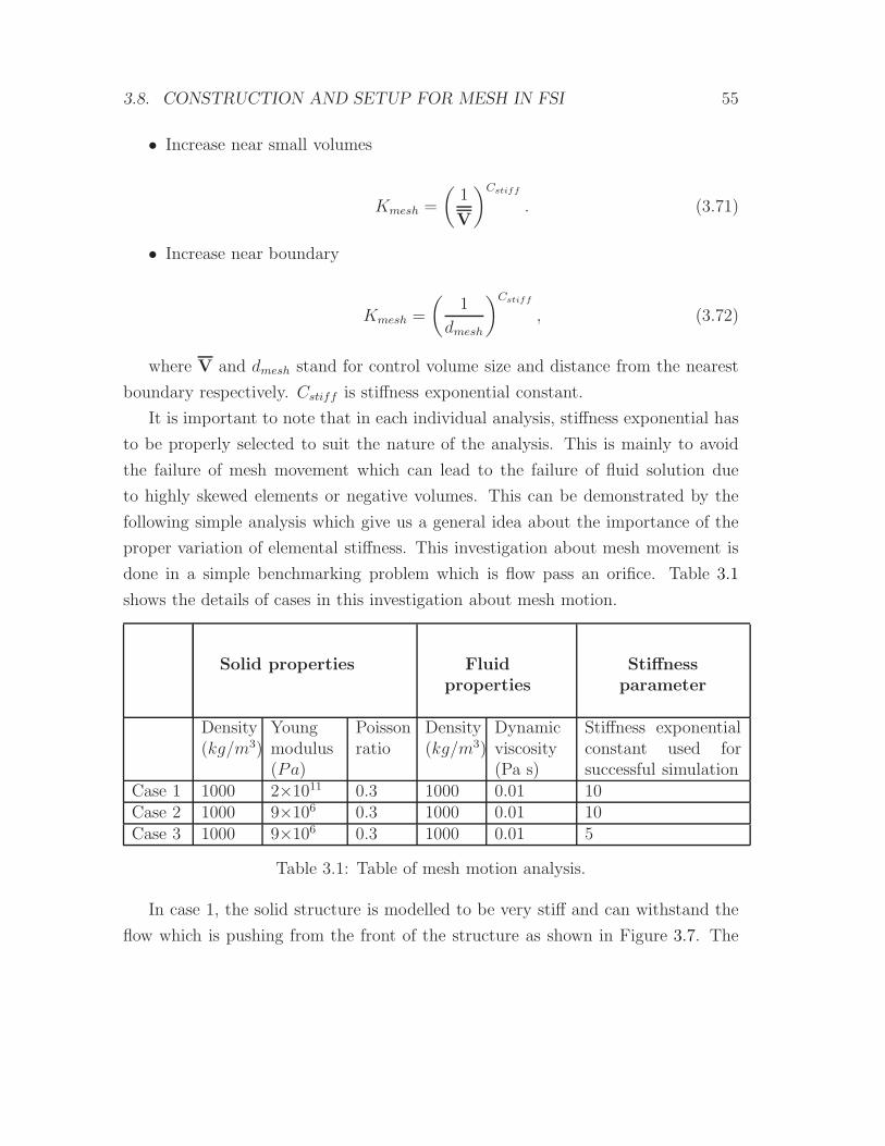
3.8. CONSTRUCTION AND SETUP FOR MESH IN FSI 55
• Increase near small volumes
Kmesh =
(1
V
)Cstiff
. (3.71)
• Increase near boundary
Kmesh =
(1
dmesh
)Cstiff
, (3.72)
where V and dmesh stand for control volume size and distance from the nearest
boundary respectively. Cstiff is stiffness exponential constant.
It is important to note that in each individual analysis, stiffness exponential has
to be properly selected to suit the nature of the analysis. This is mainly to avoid
the failure of mesh movement which can lead to the failure of fluid solution due
to highly skewed elements or negative volumes. This can be demonstrated by the
following simple analysis which give us a general idea about the importance of the
proper variation of elemental stiffness. This investigation about mesh movement is
done in a simple benchmarking problem which is flow pass an orifice. Table 3.1
shows the details of cases in this investigation about mesh motion.
Solid properties Fluid
properties
Stiffness
parameter
Density(kg/m3)
Youngmodulus(Pa)
Poissonratio
Density(kg/m3)
Dynamicviscosity(Pa s)
Stiffness exponentialconstant used forsuccessful simulation
Case 1 1000 2×10¹¹ 0.3 1000 0.01 10Case 2 1000 9×10⁶ 0.3 1000 0.01 10Case 3 1000 9×10⁶ 0.3 1000 0.01 5
Table 3.1: Table of mesh motion analysis.
In case 1, the solid structure is modelled to be very stiff and can withstand the
flow which is pushing from the front of the structure as shown in Figure 3.7. The
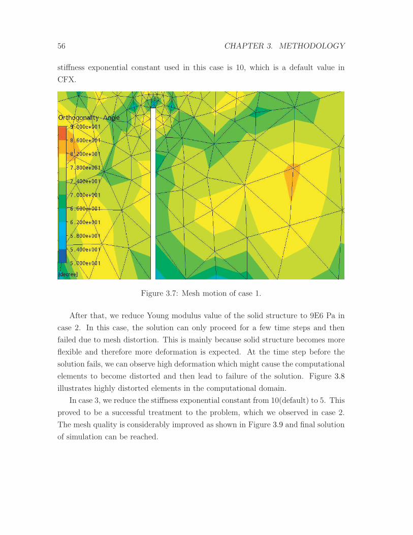
56 CHAPTER 3. METHODOLOGY
stiffness exponential constant used in this case is 10, which is a default value in
CFX.
Figure 3.7: Mesh motion of case 1.
After that, we reduce Young modulus value of the solid structure to 9E6 Pa in
case 2. In this case, the solution can only proceed for a few time steps and then
failed due to mesh distortion. This is mainly because solid structure becomes more
flexible and therefore more deformation is expected. At the time step before the
solution fails, we can observe high deformation which might cause the computational
elements to become distorted and then lead to failure of the solution. Figure 3.8
illustrates highly distorted elements in the computational domain.
In case 3, we reduce the stiffness exponential constant from 10(default) to 5. This
proved to be a successful treatment to the problem, which we observed in case 2.
The mesh quality is considerably improved as shown in Figure 3.9 and final solution
of simulation can be reached.
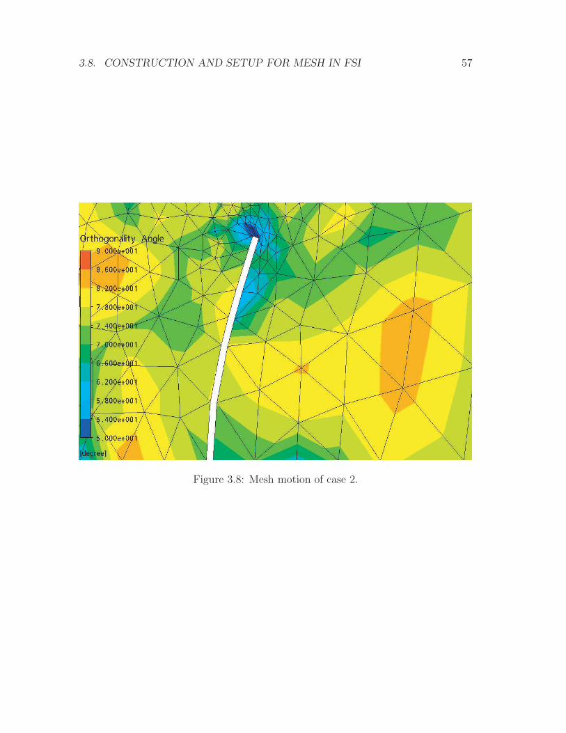
3.8. CONSTRUCTION AND SETUP FOR MESH IN FSI 57
Figure 3.8: Mesh motion of case 2.

58 CHAPTER 3. METHODOLOGY
Figure 3.9: Mesh motion of case 3.
3.9. SUMMARY AND CONCLUDING REMARKS 59
From the above investigation, it can be pointed out that elemental stiffness of
computational domain should be properly set up by considering the deformation, is
expected to occur during simulation. From both equations above, the larger Cstiff
will lead to a larger stiffness gradient. And we can also expect that large stiffness
gradient will cause negative volume and folded mesh. This can be explained by
considering two adjacent elements, one moves significantly but the other element
does not move (or slightly move), then the element that moves significantly will fold
onto the other one. It may be a straight forward idea to reduce the Cstiff to smooth
out the mesh whenever we get the mesh folding or negative volume due to large
deformation. However, the lack of accuracy due to this small value of Cstiff may
affect our result. This is due to the structure not experiencing significantly large
deformation but the mesh stiffness gradient is chosen to be small; the quality of
mesh surrounding the solid structure at interface becomes slightly lower compared
to that when we have higher Cstiff . To optimize this, an expression was suggested
in (Solving FSI Applications using Workbench, ANSYS Mechanical and CFX, n.d.)
as follows.
Cstiff = 1−(
wall distance −minimum value of wall distance
maximum value of wall distance−minimum value of wall distance
)2
.
(3.73)
3.9 Summary and concluding remarks
This chapter provides detailed information about governing equations and method-
ology incluing discretization schemes used for both fluid and solid solver. Also,
calculation procedures corresponding to techniques are discussed. Moreover, best
practice in FSI based on the author’s knowledge and experience is suggested.

60 CHAPTER 3. METHODOLOGY
Chapter 4
Theoretical analysis of stability in
FSI
4.1 Introduction
Fluid-structure interaction is used widely in many engineering fields such as Auto-
motive, Biomechanical and Aerospace engineering. It can be done in mainly two
approaches: Monolithic and Partitioned approach. FSI solvers, when using the first
approach, solves a system of governing equations of both fluid and solid fields (Hron
and Turek, 2006). Although it gives strong coupling between the fields, the short-
comings are the following.
• Demanding computational power for solving a large system of equations
• The need for further development preconditioning
• Lack of specialized capabilities of the sophisticated software such as ABAQUS
and ANSYS.
On the other hand, the partitioned approach is attractive due to its advan-
tage of software modularity allowing selection of an appropriate solver among well-
established solvers for each field. However, the efficiency of partitioned approach
61
62 CHAPTER 4. THEORETICAL ANALYSIS OF STABILITY IN FSI
is inferior to the other approach due to the existence of the so-called “Added-mass
instability” which commonly occurs in problems with large deformation and light
weight structure. This can cause FSI solution to diverge and fail before the final
solution is reached. In order to handle this instability, small values of coupling
relaxation factors of interface loads must be used in order to maintain stability of
calculation. This leads to a significant increase in computational time. It is under-
stood that FSI solution experiences this numerical instability when the following
conditions is observed (Forster et al., 2007).
• Stability of FSI solution tends to be highly severe when density ratio between
fluid and solidρfρs
is high.
• The increase in fluid viscosity leads to increased instability. In contrast, the
increase in structural stiffness results in less instability.
• Temporal discretisation schemes used for FSI calculation could influence the
condition of instability.
• The decrease in time step size used for FSI calculation make instability occur
earlier.
The observed behaviours of the instability is explained mathematically by Causin
et al. (2005) where conditions for stability of both explicit and implicit FSI solution
of a flexible cylindrical vessel are demonstrated. However, impact of structural time
integration scheme, which is used for FSI calculation, is still not fully understood.
The main aim of this chapter is to analyze performance of FSI using partitioned
approach based on different structural time integration schemes. We conduct the
analysis on a simplified problem of pressure wave propagation along a flexible cylin-
drical vessel. Our findings can be summarized as follows.
• Influence of structural time integration schemes on performance of FSI
• Influence of time step size
• Influence of density ratio
4.2. SIMPLIFIED PROBLEM FOR STABILITY ANALYSIS 63
• Influence of geometric properties
Moreover, a theoretical analysis of FSI coupling using artificial compressibility
is also discussed and compared with those using under-relaxation technique. This
chapter is organized as follows. In Section 2, a mathematical description of a sim-
plified pressure wave propagation along a flexible cylindrical vessel and fundamental
FSI conditions are presented. In Section 3, theoretical analysis of stability based on
under-relaxation technique are discussed.
4.2 Simplified problem for stability analysis
A simple flexible cylindrical tube is chosen for our mathematical analysis. It allows
mathematical and numerical studies to be performed, and provides enough infor-
mation for conducting a more realistic situation. A schematic representation of our
problem domain is shown in Figure 4.1.
Deformation of the cylindrical tube is allowed only in the radial and longitudinal
directions. Inlet and outlet of the fluid domain are subjected to pressure boundary
conditions. We refer to governing equation of deformation of a flexible cylindrical
tube in the work by Causin et al. (2005), which can be written as
ρshs
∂2dΓ∂t2
+ a0dΓ − b∂2dΓ∂x2
= PΣ,Γ, (4.1)
ρshs
∂2dΓ∂t2
+ a0dΓ − b∂2dΓ∂x2
= Pext,Γ − ρfMa
∂2dΓ∂t2
, (4.2)
ρshs
∂2dΓ∂t2
+ ρfMa
∂2dΓ∂t2
+ a0dΓ − b∂2dΓ∂x2
= Pext,Γ, (4.3)
where a0 =Ehs
r2(1−ν2), b = KTBhs, x is position in space and t is position in time.
Since we are interested in added-mass instability, where the mass term is dom-
inated the stiffness term, we will neglect some non-linearity. Therefore, (4.3) is
reduced to equation (4.4) such that
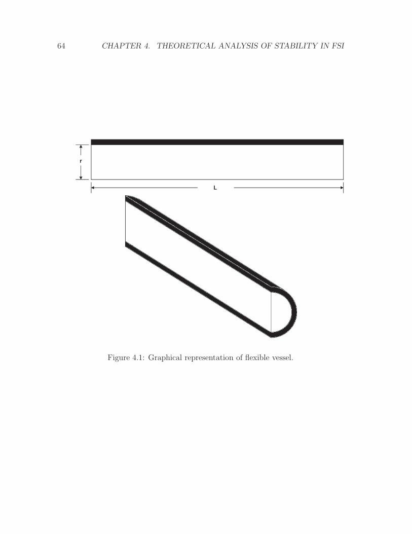
64 CHAPTER 4. THEORETICAL ANALYSIS OF STABILITY IN FSI
L
r
Figure 4.1: Graphical representation of flexible vessel.
4.3. THEORETICAL ANALYSIS: UNDER-RELAXATION 65
ρshs
∂2dsΓ∂t2
+ ρfMa
∂2dfΓ∂t2
+ a0dsΓ = Pext,Γ. (4.4)
4.3 Theoretical analysis: under-relaxation
A stability analysis of FSI calculation using implicit coupling is presented. By
adopting implicit coupling, several coupling iterations are needed for each time step
and relaxation is applied to maintain the stability of calculation.
4.3.1 Stability condition: minimum numerical damping is
applied
In this section, the analysis of explicit FSI coupling, when minimum numerical
damping is used, is discussed.
The discretized form of structural acceleration is written as
dn+1,sΓ ≈ 1
4t2(4dn+1
Γ − 16dnΓ + 32dn−1Γ − 20dn−2
Γ
)− 12
4tdn−2Γ − dn−2
Γ . (4.5)
The discretized form of fluid acceleration is written as
dn+1,fΓ = 1
∆t2(dn+1
Γ − 2dnΓ + dn−1Γ ). (4.6)
Unlike explicit coupling, the latest information used for calculation of FSI inter-
face acceleration of fluid domain comes from the same time level with that used for
structural acceleration. This is due to the application of relaxation factors.
Discretization of equation (4.4) is achieved by substituting equations (4.5) and
(4.6) to give
66 CHAPTER 4. THEORETICAL ANALYSIS OF STABILITY IN FSI
ρshs
4t2(4dn+1
Γ − 16dnΓ + 32dn−1Γ − 20dn−2
Γ − 12
4t3dn−2Γ − 1
4t2dn−2Γ )
+ρfMa
4t2(dn+1
Γ − 2dnΓ + dn−1Γ ) + a0d
n+1Γ = P n+1
ext,Γ. (4.7)
To simplify it, the analysis can be done by considering only one eigenvector, vi
of solution on the interface. This is because the added mass opertor, MA is a real
positive matrix. Therefore, dΓ = Σdivi. Notice that the added-mass operator MA
can be represented by the ith eigenvalues of MA, µi. This reduced equation (4.7) to
(4.8) as given by
ρshs
4t2(4dn+1
i − 16dni + 32dn−1i − 20dn−2
i − 12
4t3dn−2i − 1
4t2dn−2i )
+ρfµi
4t2(dn+1
i − 2dni + dn−1i ) + a0d
n+1i =
4t2
ρshs
P n+1ext,i. (4.8)
By substituting equation (3.59), equation (4.8) can be rewritten as
ρshs
4t2(4dn+1
i
ω− 16dni + 32dn−1
i − 20dn−2i − 12
4t3dn−2i − 1
4t2dn−2i ) + a0
dn+1m+1,i
ω
=
(1− ω
ω
)(2ρshs
4t2+ a0
)dn+1m,i − ρfµi
4t2(dn+1
m,i − 2dni + dn−1i ) +
4t2
ρshs
P n+1ext,i ,(4.9)
1
ω
(4ρshs
4t2+ a0
)dn+1m+1,i =
[(1− ω
ω
)(4ρshs
4t2+ a0
)− ρfµi
4t2
]dn+1m,i
+g(dni , d
n−1i , dn−2
i , dn−2i , dn−2
i , P n+1ext,i
), (4.10)
4.3. THEORETICAL ANALYSIS: UNDER-RELAXATION 67
dn+1m+1,i
dn+1m,i
≈
[(1−ωω
) (4ρshs
4t2+ a0
)− ρfµi
4t2
]
1ω
(4ρshs
4t2+ a0
) = 1− ω (4ρshs + a04t2 + ρfµi)
4ρshs + a04t2.
︸ ︷︷ ︸Growthfactor,G
(4.11)
Absolute value of the growth factor has to be less than unity if the solution is to
be stable. That is
|G| =∣∣∣∣1−
ω (4ρshs + a04t2 + ρfµmax)
4ρshs + a04t2
∣∣∣∣ < 1, (4.12)
0 < ω <8ρshs + 2a04t2
4ρshs + a04t2 + ρfµmax
. (4.13)
From equation (4.13), it is obvious that not only the material and geometrical
properites such as density of both fluid and solid, Young modulus and the maximum
eigenvalue of added mass matrix influences the allowable relaxation factor but also
the time step size of the calculation. It can be further deduced that if the time step
size is very small (approaching zero), then equation (4.13) becomes
0 < ω <8
4 +ρfµmax
ρshs
. (4.14)
This means that if time step size is very small, the Young modulus is no longer a
factor that determines the criteria for stability of an implicit algorithm. Therefore,
the critical value of relaxation factor converges and does not vary with a further
decrease in time step size. Moreover, it can also be concluded that if ρfµmax = ρshs
, then the relaxation factor has to be strictly less than 85to allow convergence of
solution.
68 CHAPTER 4. THEORETICAL ANALYSIS OF STABILITY IN FSI
4.3.2 Stability condition: maximum numerical damping is
applied
The discretized form of structural acceleration is written as
dn+1,sΓ =
1
∆t2(2dn+1
Γ − 5dnΓ + 4dn−1Γ − dn−2
Γ ). (4.15)
The discretized form of fluid acceleration is written as
dn+1,fΓ = 1
∆t2(dn+1
Γ − 2dnΓ + dn−1Γ ). (4.16)
Unlike explicit coupling, the latest information used for calculation of FSI inter-
face acceleration of fluid domain comes from the same time level as that used for
structural acceleration. This is due to the application of relaxation factors.
The discretized form of equation (4.4) is achieved by substituting equations (4.15)
and (4.16) to give
ρshs
4t2(2dn+1
Γ − 5dnΓ + 4dn−1Γ − dn−2
Γ ) +ρfMa
4t2(dn+1
Γ − 2dnΓ + dn−1Γ ) + a0d
n+1Γ
= P n+1ext,Γ, (4.17)
ρshs
4t2(2dn+1
i − 5dni + 4dn−1i − dn−2
i ) +ρfµi
4t2(dn+1
i − 2dni + dn−1i ) + a0d
n+1i
=4t2
ρshs
P n+1ext,i. (4.18)
By substituting equation (3.59), equation (4.18) can be rewritten as
4.3. THEORETICAL ANALYSIS: UNDER-RELAXATION 69
ρshs
4t2(2dn+1
m+1,i
ω− 5dni + 4dn−1
i − dn−2i ) + a0
dn+1m+1,i
ω
=
(1− ω
ω
)(2ρshs
4t2+ a0
)dn+1m,i − ρfµi
4t2(dn+1
m,i − 2dni + dn−1i )
+4t2
ρshs
P n+1ext,i , (4.19)
1
ω
(2ρshs
4t2+ a0
)dn+1m+1,i =
[(1− ω
ω
)(2ρshs
4t2+ a0
)− ρfµi
4t2
]dn+1m,i
+g(dni , d
n−1i , dn−2
i , P n+1ext,i
), (4.20)
dn+1m+1,i
dn+1m,i
≈
[(1−ωω
) (2ρshs
4t2+ a0
)− ρfµi
4t2
]
1ω
(2ρshs
4t2+ a0
) = 1− ω (2ρshs + a04t2 + ρfµi)
2ρshs + a04t2︸ ︷︷ ︸Growthfactor,G
. (4.21)
Absolute value of the growth factor has to be less than unity if the solution is to
be stable. That is
|G| =∣∣∣∣1−
ω (2ρshs + a04t2 + ρfµmax)
2ρshs + a04t2
∣∣∣∣ < 1, (4.22)
0 < ω <4ρshs + 2a04t2
2ρshs + a04t2 + ρfµmax
. (4.23)
From equation (4.23), it is obvious that not only the material and geometrical
properites such as density of both fluid and solid, Young modulus and eigenvalue
of added mass matrix has influence on the allowable relaxation factor but also the
70 CHAPTER 4. THEORETICAL ANALYSIS OF STABILITY IN FSI
time step size of the calculation. It can be further put that if the time step size is
very small (approach to zero), then equation (4.23) becomes
0 < ω <4
2 +ρfµmax
ρshs
. (4.24)
Here, it is proved that if time step size is very small, the Young modulus is
no longer a factor determining the criteria for stability of implicit algorithm. This
also means that the critical value of relaxation factor converges and does not vary
with a further decrease in time step size. Moreover, it can also be concluded that
if ρfµmax = ρshs , then the relaxation factor has to be strictly less than 43to allow
convergence of solution.
4.3.3 Generalization of stability condition
We recall equations (3.25) and (3.26) which are used as time integration method of
structural analysis.
dn+1 = dn + (1− δ)4tdn + δ4tdn+1,
dn+1 =1
α4t2
[dn+1 − dn −4tdn −
(1
2− α
)4t2dn
].
We also recall that
dα = (1− αm) dn+1 + αmd
n.
Therefore, structural acceleration can be rewritten as
dn+1,α = (1− αm)1
α4t2
[dn+1 − dn −4tdn −
(1
2− α
)4t2dn
]
+αm
α4t2
[dn − dn−1 −4tdn−1 −
(1
2− α
)4t2dn−1
]. (4.25)
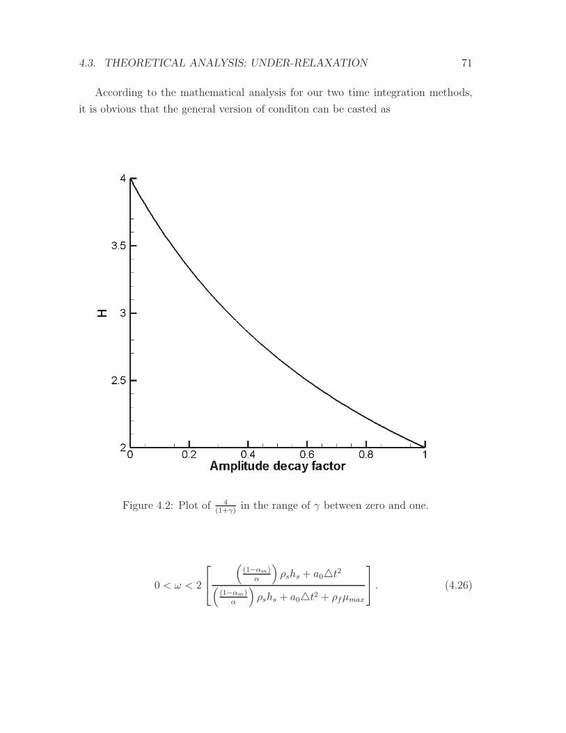
4.3. THEORETICAL ANALYSIS: UNDER-RELAXATION 71
According to the mathematical analysis for our two time integration methods,
it is obvious that the general version of conditon can be casted as
Figure 4.2: Plot of 4(1+γ)
in the range of γ between zero and one.
0 < ω < 2
((1−αm)
α
)ρshs + a04t2
((1−αm)
α
)ρshs + a04t2 + ρfµmax
. (4.26)
72 CHAPTER 4. THEORETICAL ANALYSIS OF STABILITY IN FSI
In order to optimize the stability of FSI solution using the generalized-α time
integration scheme, (1−αm)α
should be maximized. In an attempt to find the max-
imum value of this term, it is important that conditions of stability and accuracy
of structural solution are also satisfied. According to (ANSYS Inc. 2009. ANSYS
CFX-Solver Theory Guide, n.d.),
(1− αm)
α=
4
(1 + γ). (4.27)
For maintaining stability and accuracy when using the time integration method,
the following condition must be satisfied.
0 ≥ γ ≥ 1. (4.28)
4.4 Summary and concluding remarks
In practice, most of physical and numerical properties (such as dimension of problem
domain and time step size) are fixed and the combination of their contributions to
the stability of the FSI coupling may lead to divergence and failure of solution.
Therefore, it is necessary to determine the critical value of relaxation factor which
allows the solution to be stable. A similar analysis was done by Causin et al. (2005)
but in their work, only the Leap-Frog schemes are used for analysis. Here, in our
analysis, we obtain similar conclusions made by them. In our derivations, the critical
value of relaxation factor is found to be a function of the following parameters:
• Density of solid and fluid;
• Time step size;
• Young modulus of solid;
• Geometrical properties such as vessel thickness and radius.
From our derivations, the influence of these parameters can be summarized as
follows:
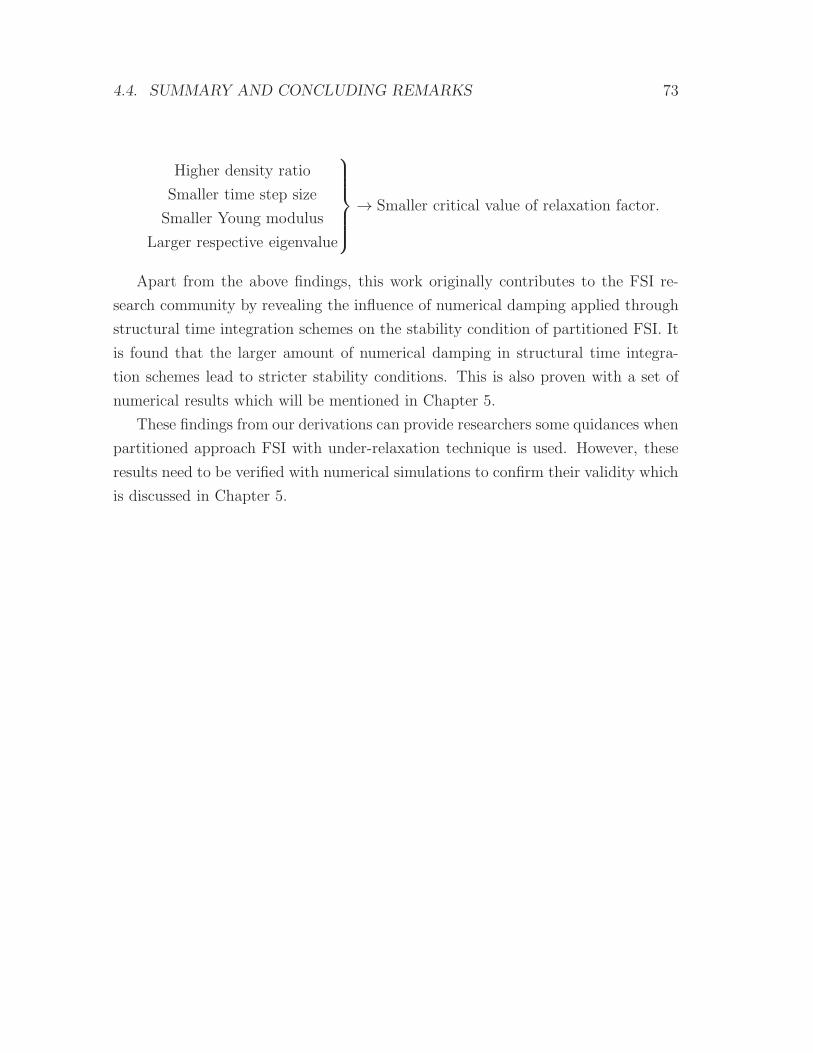
4.4. SUMMARY AND CONCLUDING REMARKS 73
Higher density ratio
Smaller time step size
Smaller Young modulus
Larger respective eigenvalue
→ Smaller critical value of relaxation factor.
Apart from the above findings, this work originally contributes to the FSI re-
search community by revealing the influence of numerical damping applied through
structural time integration schemes on the stability condition of partitioned FSI. It
is found that the larger amount of numerical damping in structural time integra-
tion schemes lead to stricter stability conditions. This is also proven with a set of
numerical results which will be mentioned in Chapter 5.
These findings from our derivations can provide researchers some quidances when
partitioned approach FSI with under-relaxation technique is used. However, these
results need to be verified with numerical simulations to confirm their validity which
is discussed in Chapter 5.

74 CHAPTER 4. THEORETICAL ANALYSIS OF STABILITY IN FSI
Chapter 5
Validation and numerical results
In this chapter, a series of numerical tests conducted on both under-relaxation tech-
nique and artificial compressibility methods implementing fluid-structure interac-
tion problems and using the different time integration method discussed in previous
chapters are presented. The main purpose of these tests is to provide a numeri-
cal validation of the theoretical results mentioned in Chapter 4. Every sensitivity
analysis in this chapter was obtained in the time interval [0, Tmax = 0.011s].
5.1 Validation
In this section a validation is proveded for justifing the accuracy of the relaxation
factor technique and artificial compressibility used in this work. Pressure pulse
velocity has been widely used as an indicator of blood vessel health. In the past, only
physical experiment and analytical solutions are available for obtaining the pulse
velocity. Although these analytical solutions are only used for simple geometries of
blood vessel, they can serve as solid verification for numerical simulation, which are
becoming popular nowadays. Therefore, a simulation of fluid-structure interaction
for calculating pressure pulse velocity in a compliant vessel is conducted to verify
our numerical results by comparing with analytical solutions such as the Moen-
Korteweg equation. The results presented in this section are obtained by using the
75
76 CHAPTER 5. VALIDATION AND NUMERICAL RESULTS
same method as that used in the next section where numerical results are presented
to confirm our theoretical results.
5.1.1 Geometric and material descriptions
The geometrical model of three-dimensional tube is shown in Figure 4.1. The cylin-
drical domain has a radius of 0.0005 m and a total length of 0.06 m. The working
fluid is modelled as incompressible fluid with fluid viscosity and density of 0.01 Pa ·sand 1,000 kg
m3 respectively. On the other hand, the compliant vessel is modelled as
isotropic material with Poisson ratio and density of 0.3 and 1,000 kg
m3 respectively.
Young modulus of the solid structure is varied between 50 and 200 kPa.
5.1.2 Computational domain
Figure 6.3 shows the computational mesh of both solid and fluid domains which
consist of 1,800 and 24,674 elements respectively. In the fluid mesh, the laminar
boundary layer has 5 layers of thin hexagonal elements, while 4 layers is used for
the thickness of solid domain. In this work, only one set of computational grids are
used for obtaining numerical results as our main aim is to validate the theoretical
results mentioned above.
5.1.3 Analytical solutions
In this section, analytical solutions developed for pressure wave velocity are discussed
below.
Moen-Korteweg equation
The Moen-Korteweg equation (Korteweg, 1878; Moens, 1878) can be written as
c =
√Ehs
2Rsρs, (5.1)
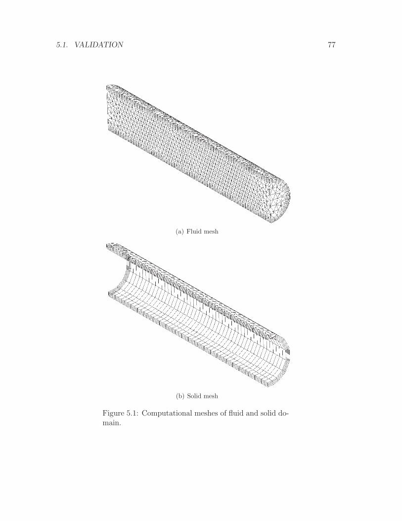
5.1. VALIDATION 77
(a) Fluid mesh
(b) Solid mesh
Figure 5.1: Computational meshes of fluid and solid do-main.
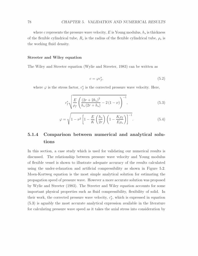
78 CHAPTER 5. VALIDATION AND NUMERICAL RESULTS
where c represents the pressure wave velocity, E is Young modulus, hs is thickness
of the flexible cylindrical tube, Rs is the radius of the flexible cylindrical tube, ρs is
the working fluid density.
Streeter and Wiley equation
The Wiley and Streeter equation (Wylie and Streeter, 1983) can be written as
c = ϕc∗f , (5.2)
where ϕ is the stress factor, c∗f is the corrected pressure wave velocity. Here,
c∗f
√√√√E
ρf
((2r + 2hs)
2
hs (2r + hs)− 2 (1− ν)
)−1
, (5.3)
ϕ =
√
1− ν2
[1− E
K
(hs
2r
)(1− Kρf
Eρs
)]−1
. (5.4)
5.1.4 Comparison between numerical and analytical solu-
tions
In this section, a case study which is used for validating our numerical results is
discussed. The relationship between pressure wave velocity and Young modulus
of flexible vessel is shown to illustrate adequate accuracy of the results calculated
using the under-relaxation and artificial compressibility as shown in Figure 5.2.
Moen-Kortweg equation is the most simple analytical solution for estimating the
propagation speed of pressure wave. However a more accurate solution was proposed
by Wylie and Streeter (1983). The Streeter and Wiley equation accounts for some
important physical properties such as fluid compressibility, flexibility of solid. In
their work, the corrected pressure wave velocity, c∗f , which is expressed in equation
(5.3) is aguably the most accurate analytical expression available in the literature
for calculating pressure wave speed as it takes the axial stress into consideration by
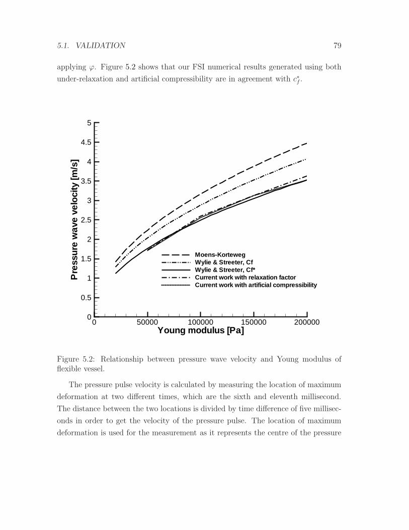
5.1. VALIDATION 79
applying ϕ. Figure 5.2 shows that our FSI numerical results generated using both
under-relaxation and artificial compressibility are in agreement with c∗f .
Young modulus [Pa]
Pre
ssur
ew
ave
velo
city
[m/s
]
0 50000 100000 150000 2000000
0.5
1
1.5
2
2.5
3
3.5
4
4.5
5
Moens-KortewegWylie & Streeter, CfWylie & Streeter, Cf*Current work with relaxation factorCurrent work with artificial compressibility
Figure 5.2: Relationship between pressure wave velocity and Young modulus offlexible vessel.
The pressure pulse velocity is calculated by measuring the location of maximum
deformation at two different times, which are the sixth and eleventh millisecond.
The distance between the two locations is divided by time difference of five millisec-
onds in order to get the velocity of the pressure pulse. The location of maximum
deformation is used for the measurement as it represents the centre of the pressure
80 CHAPTER 5. VALIDATION AND NUMERICAL RESULTS
wave. Figures 5.3 and 5.4 shows the contour plot of pressure wave propagation along
the flexible cylindrical vessel at various Young modulus and simulation time levels.
5.2 Numerical results
In this section, we present a set of numerical results with different structural time
integration scheme by varying the amplitude decay factor. The main purpose of
these results is to confirm our theoretical results. In our default configuration, which
is used as a reference to compare with other cases, we set vessel radius r = 0.005 m,
vessel lenght L=0.06 m, vessel thickness hs=0.001 m, solid density ρs=30,000 kg
m3 ,
Young modulus E = 750,000 Pa, Poisson ratio ν = 0.5, fluid density ρf=1,000 kg
m3
and fluid dynamic viscosity µf = 0.01 Pa · s. At initial condition, fluid is set to be
at rest and pressure pulse with peak of 2,000 Pa is imposed at the inlet. The total
duration of our observation, Tmax for instability is 0.02 second for different values of
amplitude decay factor γ. In the majority of test cases, the instability occurs at the
beginning of the calculation before reaching Tmax. In our results, fluid acceleration
is discretized by the second order accurate backward Euler scheme except for those
results presented in Table 5.2, which is obtained by the use of the first order accurate
backward Euler scheme and for illustrating the influence of numerical schemes used
for fluid acceleration.
5.2.1 Influence of structural time integration scheme
We observe a significant dependence on the amplitude decay factor, and namely the
required relaxation factor for maintaining stability becomes greater as the amplitude
decay factor approaches zero whereby the structural time integration sheme becomes
the average acceleration method. The numerical tests agree with our theoretical
results. In particular, they confirm that the critical relaxation factor increases with
the decrease of the structural amplitude decay factor. Moreover, it is observed that
the required values of relaxation factor when using amplitude decay factor of zero
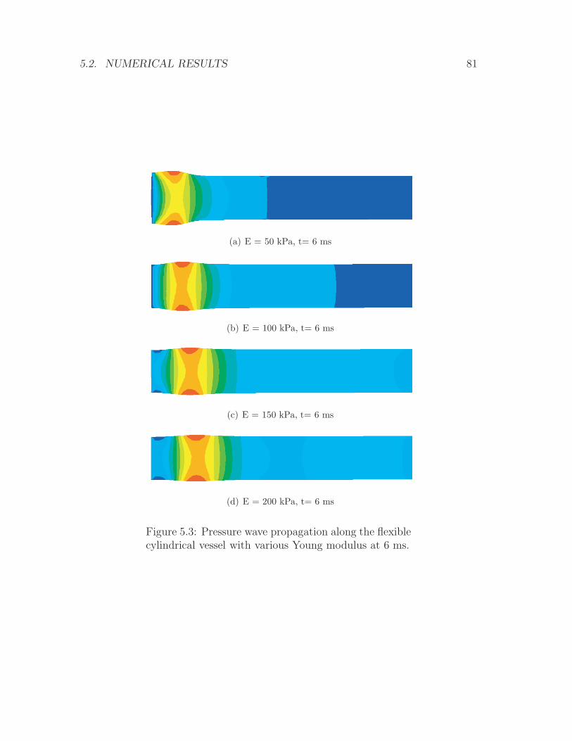
5.2. NUMERICAL RESULTS 81
(a) E = 50 kPa, t= 6 ms
(b) E = 100 kPa, t= 6 ms
(c) E = 150 kPa, t= 6 ms
(d) E = 200 kPa, t= 6 ms
Figure 5.3: Pressure wave propagation along the flexiblecylindrical vessel with various Young modulus at 6 ms.
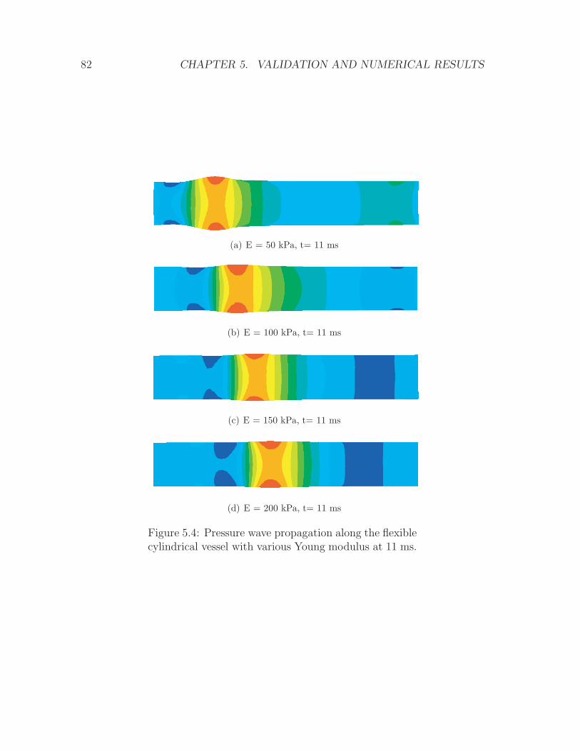
82 CHAPTER 5. VALIDATION AND NUMERICAL RESULTS
(a) E = 50 kPa, t= 11 ms
(b) E = 100 kPa, t= 11 ms
(c) E = 150 kPa, t= 11 ms
(d) E = 200 kPa, t= 11 ms
Figure 5.4: Pressure wave propagation along the flexiblecylindrical vessel with various Young modulus at 11 ms.
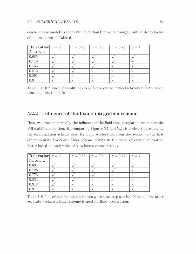
5.2. NUMERICAL RESULTS 83
can be approximately 30 percent higher than that when using amplitude decay factor
of one as shown in Table 6.1.
Relaxation
factor, ωγ = 0 γ = 0.25 γ = 0.5 γ = 0.75 γ = 1
0.685√ √ √ √ √
0.716√ √ √ √
x0.756
√ √ √x x
0.812√ √
x x x0.891
√x x x x
0.9 x x x x x
Table 5.1: Influence of amplitude decay factor on the critical relaxation factor whentime step size is 0.001s.
5.2.2 Influence of fluid time integration scheme
Here, we prove numerically the influence of the fluid time integration scheme on the
FSI stability condition. By comparing Figures 6.1 and 5.2 , it is clear that changing
the discretization scheme used for fluid acceleration from the second to the first
order accurate backward Euler scheme results in the value of critical relaxation
factor based on each value of γ to increase considerably.
Relaxation
factor, ωγ = 0 γ = 0.25 γ = 0.5 γ = 0.75 γ = 1
0.691√ √ √ √ √
0.728√ √ √ √
x0.776
√ √ √x x
0.834√ √
x x x0.913
√x x x x
0.9 x x x x x
Table 5.2: The critical relaxation factors when time step size is 0.001s and first orderaccurate backward Euler scheme is used for fluid acceleration.
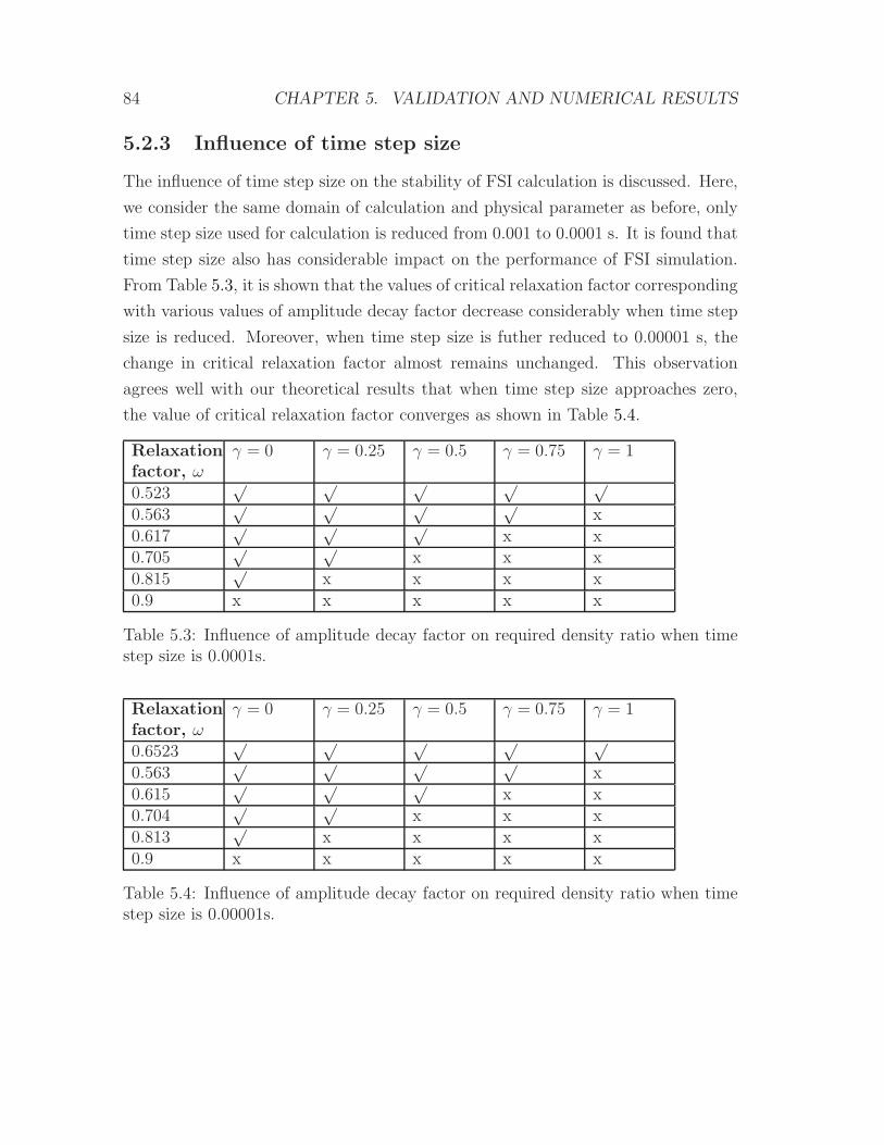
84 CHAPTER 5. VALIDATION AND NUMERICAL RESULTS
5.2.3 Influence of time step size
The influence of time step size on the stability of FSI calculation is discussed. Here,
we consider the same domain of calculation and physical parameter as before, only
time step size used for calculation is reduced from 0.001 to 0.0001 s. It is found that
time step size also has considerable impact on the performance of FSI simulation.
From Table 5.3, it is shown that the values of critical relaxation factor corresponding
with various values of amplitude decay factor decrease considerably when time step
size is reduced. Moreover, when time step size is futher reduced to 0.00001 s, the
change in critical relaxation factor almost remains unchanged. This observation
agrees well with our theoretical results that when time step size approaches zero,
the value of critical relaxation factor converges as shown in Table 5.4.
Relaxation
factor, ωγ = 0 γ = 0.25 γ = 0.5 γ = 0.75 γ = 1
0.523√ √ √ √ √
0.563√ √ √ √
x0.617
√ √ √x x
0.705√ √
x x x0.815
√x x x x
0.9 x x x x x
Table 5.3: Influence of amplitude decay factor on required density ratio when timestep size is 0.0001s.
Relaxation
factor, ωγ = 0 γ = 0.25 γ = 0.5 γ = 0.75 γ = 1
0.6523√ √ √ √ √
0.563√ √ √ √
x0.615
√ √ √x x
0.704√ √
x x x0.813
√x x x x
0.9 x x x x x
Table 5.4: Influence of amplitude decay factor on required density ratio when timestep size is 0.00001s.
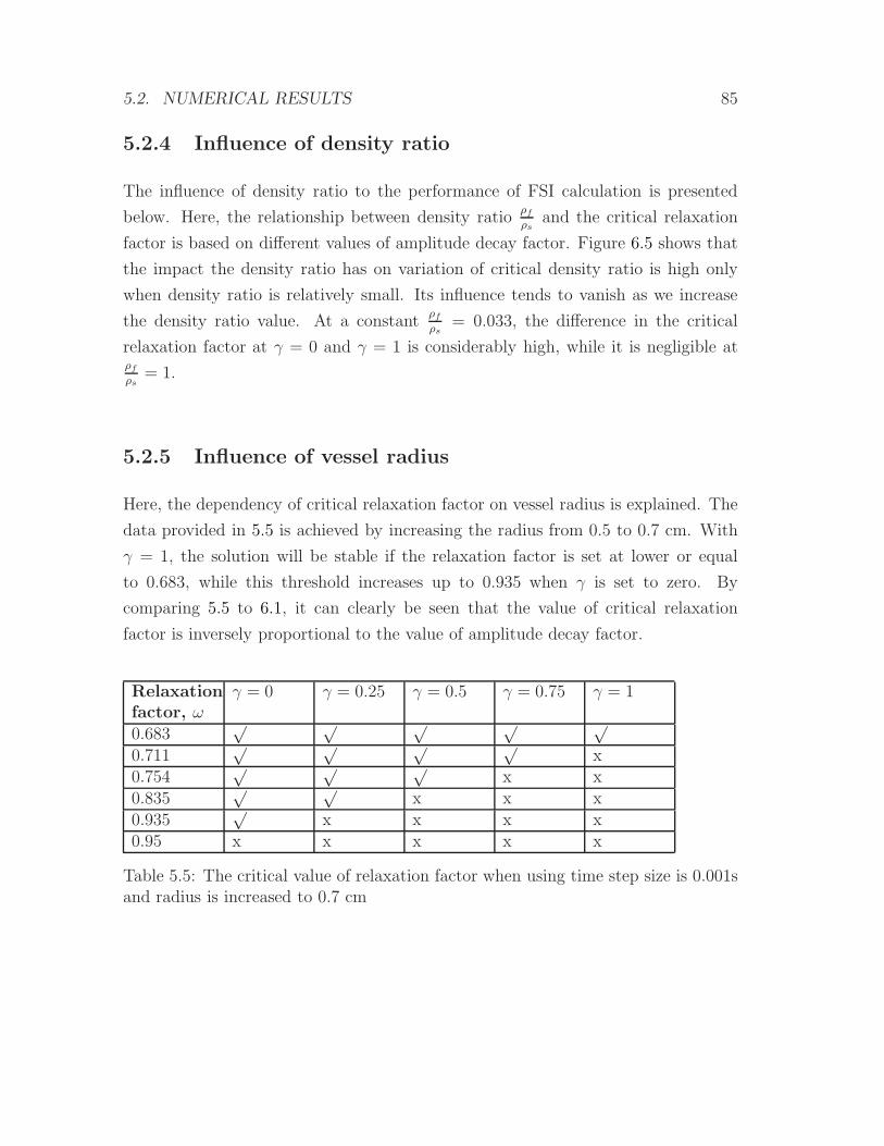
5.2. NUMERICAL RESULTS 85
5.2.4 Influence of density ratio
The influence of density ratio to the performance of FSI calculation is presented
below. Here, the relationship between density ratioρfρs
and the critical relaxation
factor is based on different values of amplitude decay factor. Figure 6.5 shows that
the impact the density ratio has on variation of critical density ratio is high only
when density ratio is relatively small. Its influence tends to vanish as we increase
the density ratio value. At a constantρfρs
= 0.033, the difference in the critical
relaxation factor at γ = 0 and γ = 1 is considerably high, while it is negligible atρfρs
= 1.
5.2.5 Influence of vessel radius
Here, the dependency of critical relaxation factor on vessel radius is explained. The
data provided in 5.5 is achieved by increasing the radius from 0.5 to 0.7 cm. With
γ = 1, the solution will be stable if the relaxation factor is set at lower or equal
to 0.683, while this threshold increases up to 0.935 when γ is set to zero. By
comparing 5.5 to 6.1, it can clearly be seen that the value of critical relaxation
factor is inversely proportional to the value of amplitude decay factor.
Relaxation
factor, ωγ = 0 γ = 0.25 γ = 0.5 γ = 0.75 γ = 1
0.683√ √ √ √ √
0.711√ √ √ √
x0.754
√ √ √x x
0.835√ √
x x x0.935
√x x x x
0.95 x x x x x
Table 5.5: The critical value of relaxation factor when using time step size is 0.001sand radius is increased to 0.7 cm
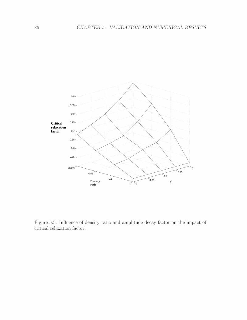
86 CHAPTER 5. VALIDATION AND NUMERICAL RESULTS
0
0.25
0.5
0.75
1
0.033
0.05
0.1
1
0.55
0.6
0.65
0.7
0.75
0.8
0.85
0.9
γDensityratio
Critical relaxation factor
Figure 5.5: Influence of density ratio and amplitude decay factor on the impact ofcritical relaxation factor.
5.3. IMPLICIT SOLUTION USING ARTIFICIAL COMPRESSIBILITY 87
5.3 Implicit solution using artificial compressibil-
ity
In this section, numerical results are used to validate our theoretical results, which
suggests that FSI coupling based on artificial compressiblity is unconditionally sta-
ble. It is found that the FSI coupling is stable regardless of the following factors that
commonly affect stability of coupling if it is based on under-relaxation technique.
• applied numerical damping
• density ratio
• time step size
• geometrical properties such as radius and thickness of vessel
The only factor that dictates the success of FSI coupling using artificial com-
pressibility is the relationship between deformation and pressure, Kac. Therefore,
the selection of this value is critical. The calculation of this parameter was suggested
in the work by Raback et al. (2001). We recall from Figure 5.2 that the results
obtained by using artificial compressibility are close to those of under-relaxation
technique.
5.4 Performance comparision between artificial com-
pressibility and under-relaxation technique
Apart from being applicable to solving problems with higher density ratio, artificial
compressibility has a superior performance to the under-relaxation technique when
solving the wave propagation along a flexible cylindrical tube as shown in Table 5.6.
This comparison is achieved by looking at the computational time required for solv-
ing the problem between the two techniques. The total time and time step size are
11 and 1 ms respectively. For each case, no numerical damping is applied since it
88 CHAPTER 5. VALIDATION AND NUMERICAL RESULTS
has been proven that it performs best with no numerical damping. For cases with
artificial compressibility, Kac are chosen according to the work done by Raback et al.
(2001). In each case, convergence of interface loads are satisfied by allowing enough
coupling iterations. Density of fluid is fixed at 1000 kg
m3 while density of solid is var-
ied according to the density ratio. Young modulus and poisson ratio of the tube is
held constant at 0.75 MPa and 0.49 respectively. Each case is run on a workstation
with Intel duo core2 CPU (3.16 GHz) which has 3.48 Gigabyte of RAM. The same
set of computational meshes mentioned in Section 5.1.2 are used for each case.
From Table 5.6, as we increase the density ratio from 0.033 to 1.0, the com-
putational time required for computing with under-relaxation technique increases
dramatically from 19 minutes and 8 seconds to almost 15 hours. This trend re-
lates to the decrease of critical value of relaxation factor that allow stable solution
which leads to a larger number of coupling iterations needed for reaching conver-
gence criteria. In contrast, the computational time of those cases using artificial
compressibility only rise slightly from 19 minutes and 38 seconds to 30 minutes and
43 seconds. With this methods, there is only a small change in the average of re-
quired number of coupling iteractions from 3.27 to 5.00. It is therefore clear that
artificial compressibility is a more efficient method for solving problems with high
density ratio than the under-relaxation technique.
However, it should be noted that at a low density ratio such as 0.033 and 0.05,
the computing time when using under-relaxation technique is slightly smaller than
when using artificial compressibility, even though the averaged required numbers of
coupling iterations per time step for artificial compressibility is much smaller than
those of under-relaxation technique. This is because artificial compressiblity requires
more time for calculation and data storage process in each iteration.
5.5 Summary and concluding remarks
In this chapter, a number of simulations are conducted to confirm our theoretical
results in Chapter 4. In Chapter 4, pressure wave propagation in a straight flexible
vessel, which is a phenomenon relevant in many engineering applications such as flow
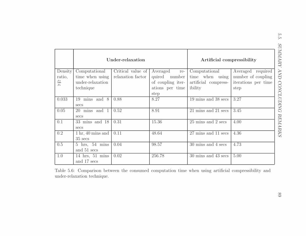
5.5.
SUMMARY
AND
CONCLUDIN
GREMARKS
89
Under-relaxation Artificial compressibility
Densityratio,ρfρs
Computationaltime when usingunder-relaxationtechnique
Critical value ofrelaxation factor
Averaged re-quired numberof coupling iter-ations per timestep
Computationaltime when usingartificial compress-ibility
Averaged requirednumber of couplingiterations per timestep
0.033 19 mins and 8secs
0.88 8.27 19 mins and 38 secs 3.27
0.05 20 mins and 1secs
0.52 8.91 21 mins and 21 secs 3.45
0.1 33 mins and 18secs
0.31 15.36 25 mins and 2 secs 4.00
0.2 1 hr, 40 mins and35 secs
0.11 48.64 27 mins and 11 secs 4.36
0.5 5 hrs, 54 minsand 51 secs
0.04 98.57 30 mins and 4 secs 4.73
1.0 14 hrs, 51 minsand 17 secs
0.02 256.78 30 mins and 43 secs 5.00
Table 5.6: Comparison between the consumed computation time when using artificial compressibility andunder-relaxation technique.
90 CHAPTER 5. VALIDATION AND NUMERICAL RESULTS
in artery, is choosen for analyzing stability condition theoretically. In this chapter,
the same problem is solved using the numerical technique in order to confirm those
results. Our numerical outcomes appear to agree well with the theoretical ones.
These outcomes can be summarized as follows:
• Structural time integration schemes with less numerical damping allow larger
critical value of relaxation factor. However, the effect of the numerical damping
becomes neglegible when density ratio is high.
• The selection of fluid time integration schemes also has considerable influence
on the critical value of relaxation factor. It is found that the 1st order accurate
backward Euler gives better stability to FSI solution.
• Smaller time step size leads to smaller critical value of relaxation factor. How-
ever, the influence of time step size disappears when we keep reducing it to a
very small value. In other words, the critical value of relaxation factor almost
stays unchanged with the decrease in time step size when the time step size is
very small.
• Geometrical properties such as radius of vessel also has an impact on the
critical value of relaxation factor. That is when radius of the flexible vessel is
greater, the stability condition can become deteriorated.
To ensure that our method in producing these numerical results is accurate, they
are validated against a number of well-defined analytical solutions which are used to
estimate the velocity pressure wave propagation. Our results go considerably well
with them and therefore ensure the accuracy of our results.
Due to the limited improvement varying numerical damping in structural time
integration scheme, the artificial compressiblity technique is also analyzed and re-
sulted a more versatile technique for a wider range of applications as it provides a
reasonably good performance regardless of density of fluid and solid. In this tech-
nique, the only key parameter, which needs some attention from the user, is the
artificial bulk modulus and it is not restricted by physical properties of the problem.
5.5. SUMMARY AND CONCLUDING REMARKS 91
Moreover, the performance of artificial compressibility is superior to that of relax-
ation factor as shown in Table 5.6. Computational time can be reduced significantly
with this technique.
It is therefore recommended to use artificial compressibility for FSI problems with
high density ratio. In Chapter 6, this method is used for analysing Atherosclerosis
in carotid bifurcation in order to confirm its practical use. This engieering problem
is selected because it has the characteristic of high density ratio and is therefore
suitable for the purpose of demonstration of practicality of artificial compressiblity.

92 CHAPTER 5. VALIDATION AND NUMERICAL RESULTS
Chapter 6
Fluid-structure interaction in
carotid bifurcation
The main purpose of this chapter is to demonstrate the practicality of FSI with
artificial compressibility for solving challenging real world engineering applications.
In this work, fluid-structure interaction of atherosclerosis in carotid bifurcation is
selected as it poses real issues of added mass stability.
6.1 Abstract
It has been suggested that atherosclerosis in carotid bifurcation depends on flow
parameters such as wall shear stress, flow pulsatility and blood pressure. However,
it is still not clearly verified how the disease becomes aggravated when plaque ex-
periences high level of shear stress during advanced stages of this disease. Despite
the significant effect of arterial compliance on hemodynamics, most previous works
are based on the assumption of modelling a rigid vessel. In this work, fluid and
structural properties in idealistic geometries are analyzed by using fluid-structure
interaction (FSI). In our results, the relationship among blood pressure, stenotic
compression and deformation was established. It shows that high level compression
93
94CHAPTER 6. FLUID-STRUCTURE INTERACTION IN CAROTID BIFURCATION
occurs at the stenotic apex, and can potentially be responsible for plaque progres-
sion. Moreover, wall shear stress and deformation are significantly affected by the
degree of stenosis.
6.2 Introduction
6.2.1 General background of atherosclerosis
Atherosclerosis is one of the most life-threatening diseases in developed countries.
The main characteristic of this disease is the narrowing of blood vessels that results
in occlusion and thus causes insufficient supply of blood to the brain and heart (Falk,
1991; Falk, 1992). Intermittently, this can lead to ischemia and heart attack. In
Australia, stroke is the cause of 9,006 deaths which is almost 7 percent of all deaths
in 2003 (Senes, 2006). This fact has motivated a rise in stroke related research
activity to rise around the globe in the past decade. It has been well understood
that stroke, due to atherosclerosis, occurs mainly because of the deficiency of oxygen
to the brain, causing brain cells to die. One of the most relevant atherosclerotic
sites for the occurrence of stoke is carotid bifurcation. This is probably because it
consists of multiple curvilinear features, which will lead to a favoured condition of the
disease, especially, at the outer wall of the inner carotid artery (ICA) sinus (Zarins
et al., 1983; Samuel et al., 2008; Ku et al., 1985). Other components of bifurcation
are the common (CCA) and external (ECA) carotid arteries.
6.2.2 Hypothesis on the developement of artherosclerosis
There has been intensive research that focuses on finding the cause of atherscle-
rosis (e.g. Caro et al., 1971; Ku et al., 1985; Glagov et al., 1989). Although un-
derstanding the causative mechanism is still not clear, many researchers suggest
that thickening of the vessel is stimulated by low levels of wall shear stress (e.g.
Friedman et al., 1989; Lee and Chiu, 1996; Giddens et al., 1993; Kleinstreuer et al.,
2001; Nerem, 1992). It is believed that low and oscillating wall shear stress increases
6.2. INTRODUCTION 95
the risk of occurrence for the disease while high wall shear stress tends to suppress
it (Friedman et al., 1986; Giddens et al., 1993; Ku et al., 1985). However, this is
not always true since it has been discovered that the disease can also develop when
the vessel is undergoing high shear stress (Joshi et al., 2004; Wentzel et al., 2003).
An example of this occurrence is at the apex of the stenosis (at advanced stages of
the disease) and the bifurcation point. Although these two regions experience high
shear stress, plaque can still grow. Tang et al. (2008) advocates that beside low and
oscillating wall shear stress, the intramural stress of the wall may also be responsible
for the progress of plaque at advanced stages by statistically proving that there is
a negative correlation between wall thickness increment and structural stress. This
induces medical experts to look for other indicators that may have influenced this
phenomenon. Mechanical values such as Von Mises and principal stresses have been
used in the past to gain understanding of the disease (Salzar et al., 1995; Hari-
ton et al., 2007; Callaghan et al., 2009; Delfino et al., 1997; Thubrikar and Robic-
sek, 1995; Kaunas et al., 2006; Lee and Xu, 2002). It is found that high mechanical
stress occurs mainly at the bifurcation point and the bulb region of bifurcation,
which are common locations for atherosclerosis. This suggests strong correlation
between the existence of the lesion and mechanical stress (Salzar et al., 1995; Delfino
et al., 1997). However, these previous studies only focus on stress level experienced
in healthy carotid bifurcations. Therefore, an important question which remains
unanswered is “How does the mechanical stresses at these regions vary with dif-
ferent degrees of stenosis”. The answer to this question will allow us to better
understand the factors that influence the growth of plaque. Deformation pattern of
the artery is also studied by Tada and Tarbell (2005) and Ramnarine et al. (2003),
but there is no report of the relationship between deformation and atherogenesis.
6.2.3 Types of atherosclerosis
According to (Gregory and Michael, 2008), atherosclerosis can have three main
categories. The first category involves atheromatous plaque which has artheroma or
lipid pool covered with fibrous cap. The second one is a non-atheromatous plaque
96CHAPTER 6. FLUID-STRUCTURE INTERACTION IN CAROTID BIFURCATION
that consists of connective tissues with admixed smooth muscle cells. The third one
is calcified plaque. The atheromatous plaque is known to be the most common of all
three categories. This can be the important reason why in recent years, most past
studies focused on atheromatous (with lipid core) and calcified type of the disease
while literature that relate to non-atheromatous (no lipid core) remains scarce. With
limited information about non-atheromatous, it is believed that mechanical stresses
experienced by this type of plaque can be quite different from the other types.
For example, atheromatous plaque is mainly subjected to high tensile stress, while
non-atheromatous plaque is subjected to compressive stress. One may argue that
non-athermatous is rare and its behavior might be trivial. Therefore, it is important
to emphasize that even though the lipidless plaque has a low percentage of occurance
compared to other types of this disease, it cannot be ignored when considering the
total number of patients suffering from this kind of disease. This fact makes it
worthwhile to try investigating the behaviour of non-atheromatous plaque in order
to provide suitable treatment for the patients. Moreover, the study of its interaction
with blood flow may also help researchers to gain better understanding of plaque
with soft lipid.
6.2.4 Clinical implications of blood pressure and heart rate
There have been many clinical reports that suggest a relationship between heart rate
and the occurance of atherosclerotic plaque (e.g. Giannoglou et al., 2008; Tardif,
2009; Palatini, 1999). These reports recommend that patients with abnormally high
blood pressure and heart rate have a higher tendency of developing stenosis in their
blood vessels. Many studies also suggest that even a standard heart rate may be
already too high and cause atherosclerosis. Therefore, the standard range of blood
pressure for healthy blood circulation may need to be revisited. This can be done
by studying the influence of blood pressure on the characteristics (such as stresses
and blood flow pattern) of atherosclerotic plaque, which may help define a proper
range of blood pressure to avoid the development of this disease. To the best of
6.3. METHODOLOGY 97
our knowledge, none of the previous studies have developed a new range of blood
pressure to replace the current range used in medical clinics.
6.2.5 Aim and scope
This work aims to analyze how mechanical stress (such as principal stress) is influ-
enced by the degree of stenosis. This allows us to gain more understanding on the
formation and the growth of atherosclerotic plaque. The second aim is to explain
the relationship between flow characteristics (such as magnitude of hemodynamic
pressure, general flow pattern and mechanical stress). Our study focuses on non-
atheromatous plaque and utilizes idealistic geometry of carotid bifurcation. A set
of important research questions that need to be answered, can be summarized as
follows:
• What is the influence of the degree of stenosis on mechanical stress experienced
in carotid bifurcation?
• How does the pattern of blood flow change with the presence of stenosis with
different sizes?
• Is there any relationship between blood pressure, strucutural stress and defor-
mation of the lesion?
6.3 Methodology
Numerical simulation by computational fluid dynamics (CFD) has an important role
nowadays in many engineering fields such as biomechanical engineering. Many re-
search questions could not possibly be acknowledged by only physical experiments.
Despite the benefit of great accuracy, these physical experiments have many draw-
backs such as difficulties in extracting meaningful data, and cost of operation when
compared to CFD. CFD is utilized to overcome these difficulties which occurred in
research communities. Moreover, due to the rapid advancement in computer tech-
nology, the power of computing has improved significantly over the recent decades.
98CHAPTER 6. FLUID-STRUCTURE INTERACTION IN CAROTID BIFURCATION
This makes it possible to incorporate FSI in the numerical simulation and increase
the accuracy of flow results that are strongly affected by the deformation of solid.
The best example will be the interaction of the artery wall and blood flow. In this
work, FSI solutions were obtained using the partitioned approach.
6.3.1 Partitioned approach for fluid-structure interaction
In the partitioned approach, the coupling between solid and fluid solver is performed
many times per time step until the convergence of interface variables (such as dis-
placements and pressure) is reached. At each coupling loop, the calculation of blood
flow is initiated. Then, calculated pressure field is transferred and used as an applied
force in the solid solver in order to calculate deformation of the artery. However,
FSI solution using this approach is computationally demanding due to the existence
of “Added-mass instability“ (Causin et al., 2005; Wall, Gerstenberger, Gamnitzer,
Forster and Ramm, 2006; Forster et al., 2007). In order to improve its performance,
FSI coupling is stabilized by introducing “Artificial compressibility”, which will be
discussed further in this work. The tolerance for the interface variables is in the
order of 1E-4. The time step size is set to 0.015 s. Results are obtained at the 4th
heart cycle to exclude effects from initial conditions.
6.3.2 Idealistic geometry of carotid bifurcation
Physiological geometries have been widely used in the past with the help of magnetic
resonance imaging (see Xue et al., 2008; Tang, 2004; Quan et al., 2000). This type
of geometry allows the inclusion of complex structures of patient-specific carotid
bifurcation, which lead to high accuracy data for the treatment of patients. However,
in order to conduct an intensive parametric study, this type of geometry may not
be suitable due to its complex features. In contrast, it is widely accepted that
simplistic geometry can capture most of the important characteristic of the problem,
and it is also simple enough in that parametric research can be implemented (Wong
et al., 2006; Wong et al., 2010). In other words, an idealistic carotid bifurcation is
suitable for studies, which aim to find the key factors that cause and influence the
6.3. METHODOLOGY 99
disease. In past decades, this type of geometry used by numerous reseachers (e.g.
Tada and Tarbell, 2005; Perktold et al., 1991; Ku and Giddens, 1983; Ding et al.,
2001), is shown to be able to represent the reasonable flow behaviour of the carotid
bifurcation.
In this work, a realistic geometry that is used by Tada and Tarbell (2005) is
selected for the modelling of healthy carotid bifurcation as shown in Figure 6.1. In
this geometry, a region of sinus is included as the common feature found in carotid
bifurcation. Detailed dimensions of the geometry can be presented in Table 6.1. For
diseased carotid bifurcation, the location of the stenosis is assumed to be located on
the outer wall of the sinus of ICA in order to study the effect of the stenosis to the
flow as well as the occurrence of mechanical stress. The degree of stenosis is varied
by variation of the ICA diameter at the location where maximum diameter of ICA
sinus occurs.
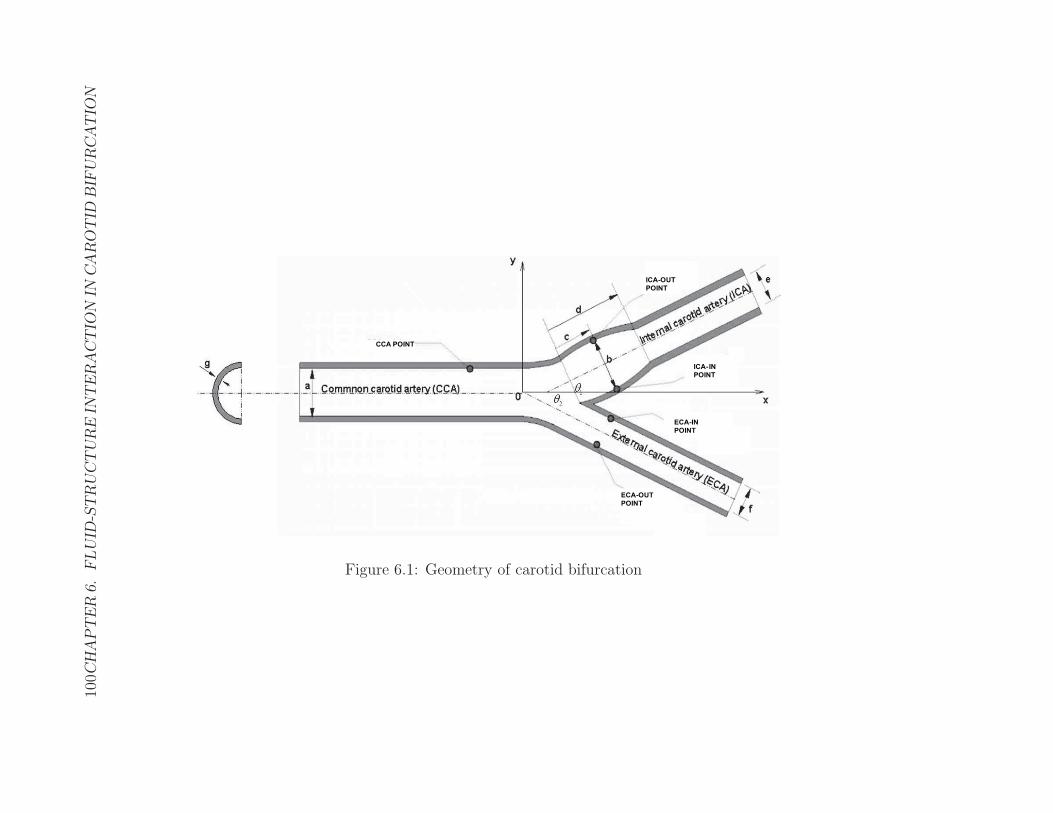
100C
HAPTER6.FLUID
-STRUCTUREIN
TERACTIO
NIN
CAROTID
BIFURCATIO
N
CCA POINT
ICA-OUT
POINT
ICA-IN
POINT
ECA-OUT
POINT
ECA-IN
POINT
Figure 6.1: Geometry of carotid bifurcation
6.3. METHODOLOGY 101
6.3.3 Computational domain
Figure 6.2 shows an example of the computational grid used in this study. In each
case, the mesh will differ slightly due to the degree of stenosis. The mesh consists of
three-dimensional tetrahedral and prism and is generated using CFX-mesh software.
Grid independence analysis was performed at 3 different mesh refinement levels:
coarse (20,000 elements), medium (500,000 elements) and fine (1,000,000 elements).
Only 2 percent of the dissimilitude between the fine and medium mesh is observed.
Therefore, it is concluded that the fine mesh can be used to obtain grid independent
results. All obtained results disserted in the discussion section are the solution of
computation performed with the fine mesh.
6.3.4 Boundary conditions and material properties
In the solid domain, each end of the artery (CCA, ICA, ECA) is modelled as fixed
support while symmetrical condition is assumed at the plane of the bifurcation. In
the fluid domain, boundary condition at the inlet is specified as a time-varying con-
stant pressure that is taken from (Tada and Tarbell, 2005), while outlet boundary
conditions at the end of ICA and ECA are set as time-varying mass flow rate as
shown in Figure 6.3. Note that the period of pressure pulse is denoted by T (in sec-
onds, s). The time t is normalized by the period of pressure pulse. In addition, no
slip condition is specified at the artery wall. The wall is assumed to be smooth. Ma-
terial models for artery wall were proposed in the past, such as the “Mooney-Rivlin”
models (Torii et al., 2009). However, in this work, the arterial wall is prepared as a
Hookian and isotropic material for simplicity as used by numerous researchers (e.g.
Salzar et al., 1995; Thubrikar and Robicsek, 1995). The blood is modelled as a
Newtonian fluid. The properties of the blood and artery are shown in Table 1. The
blood flow is modelled as a laminar flow since the highest Reynolds number, even
with high degree of stenosis, is approximately 1000 which is still in laminar region.
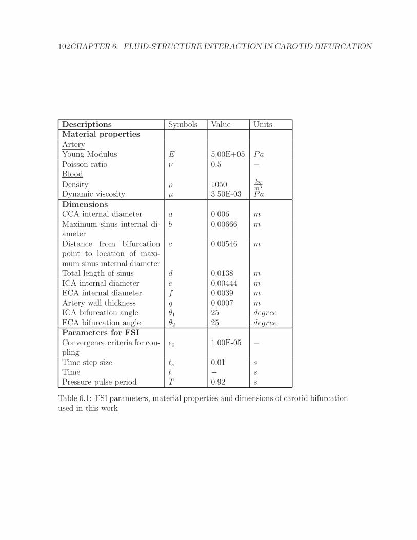
102CHAPTER 6. FLUID-STRUCTURE INTERACTION IN CAROTID BIFURCATION
Descriptions Symbols Value UnitsMaterial properties
ArteryYoung Modulus E 5.00E+05 PaPoisson ratio ν 0.5 −Blood
Density ρ 1050 kg
m3
Dynamic viscosity µ 3.50E-03 PaDimensions
CCA internal diameter a 0.006 mMaximum sinus internal di-ameter
b 0.00666 m
Distance from bifurcationpoint to location of maxi-mum sinus internal diameter
c 0.00546 m
Total length of sinus d 0.0138 mICA internal diameter e 0.00444 mECA internal diameter f 0.0039 mArtery wall thickness g 0.0007 mICA bifurcation angle θ1 25 degreeECA bifurcation angle θ2 25 degreeParameters for FSI
Convergence criteria for cou-pling
ε0 1.00E-05 −
Time step size ts 0.01 sTime t − sPressure pulse period T 0.92 s
Table 6.1: FSI parameters, material properties and dimensions of carotid bifurcationused in this work
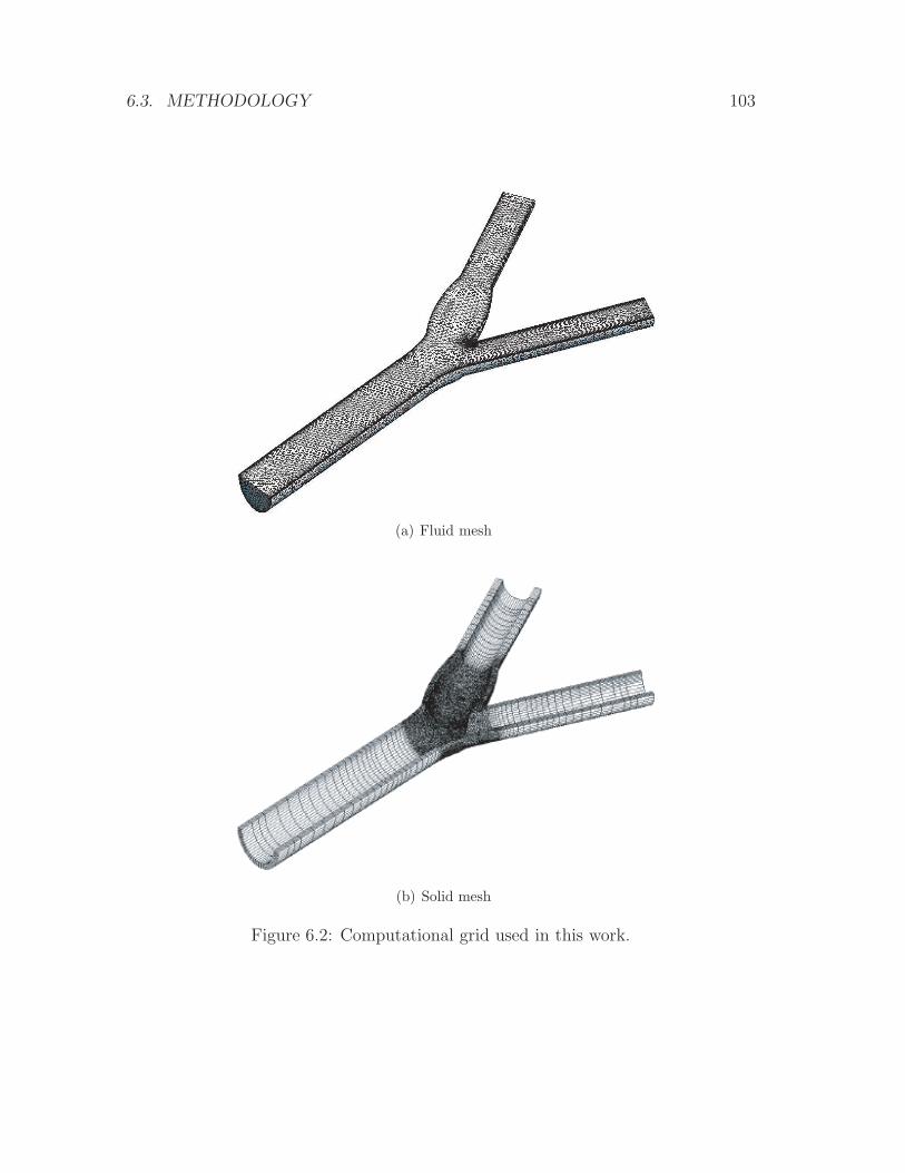
6.3. METHODOLOGY 103
(a) Fluid mesh
(b) Solid mesh
Figure 6.2: Computational grid used in this work.
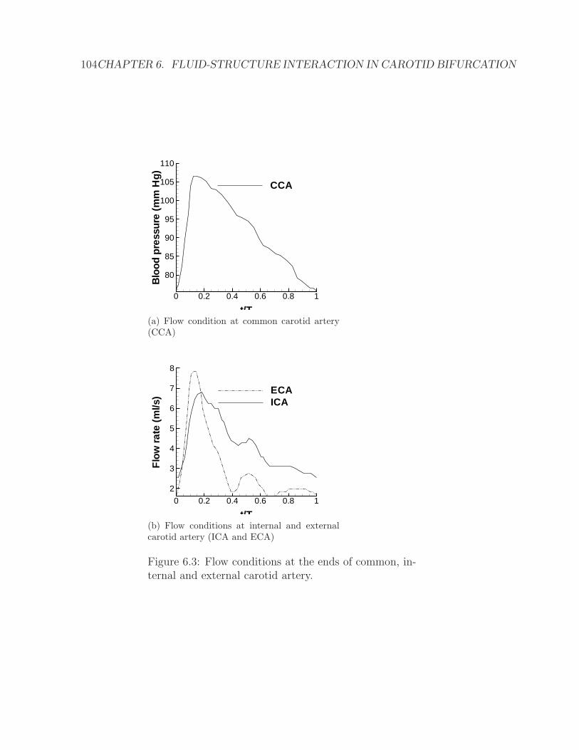
104CHAPTER 6. FLUID-STRUCTURE INTERACTION IN CAROTID BIFURCATION
t/T
Blo
odpr
essu
re(m
mH
g)
0 0.2 0.4 0.6 0.8 1
80
85
90
95
100
105
110
CCA
(a) Flow condition at common carotid artery(CCA)
t/T
Flo
wra
te(m
l/s)
0 0.2 0.4 0.6 0.8 1
2
3
4
5
6
7
8
ECAICA
(b) Flow conditions at internal and externalcarotid artery (ICA and ECA)
Figure 6.3: Flow conditions at the ends of common, in-ternal and external carotid artery.
6.4. RESULTS 105
6.3.5 Flow properties to be examined
The following mechanical parameters are examined in our work:
• Maximum principal stress (MPS) has the implication of the maximum value
of stress being applied on a vessel. The contour of MPS on the artery can
be presented using logarithmic scale. The region which has a small value
represents negative value on the linear scale. In Figure 6.7, we aim to show
the location of negative MPS on the artery, therefore only greyscale is utilized.
Positive MPS generally means that the stress is tensile whilst a negative sign
represents compression.
• Maximum deformation (MD) refers to highest possible displacement of a ves-
sel wall when it is placed under stress. This parameter has an important
implication in analysing the MPS and can be used for examining structural
vessel changes. The distribution of deformation can be used to analyse plaque
developement which is experienced by the plaque.
• Wall shear stress (WSS) is a shearing effect due to blood viscosity. We note
that wall shear stress can be oscillating due to the pulsality of blood.
• Pulse pressure refers to transient behavior of blood circulation in vessels due
to the periodic pumping action of the heart.
6.4 Results
6.4.1 Healthy carotid bifurcation – normal flow behavior
Figure 6.5(a) shows that in the healthy carotid bifurcation, the blood flow separates
at the terminal end of CCA and then forms a recirculation zone inside the ICA sinus.
The recirculation zone is located near the outer wall of the sinus, and is relatively
large when compared to the diameter of the sinus. The recirculation zone ends at
a reattachment point around the distal end of the sinus. Blood motion inside the
recirculation zone is slow and backward directing. Consequently, wall shear stress
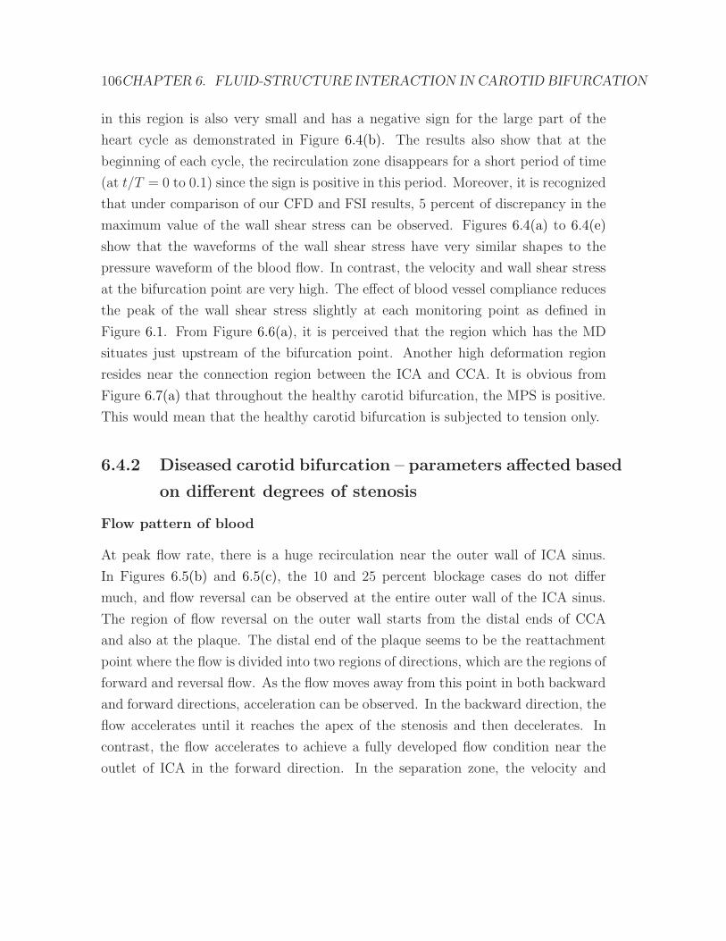
106CHAPTER 6. FLUID-STRUCTURE INTERACTION IN CAROTID BIFURCATION
in this region is also very small and has a negative sign for the large part of the
heart cycle as demonstrated in Figure 6.4(b). The results also show that at the
beginning of each cycle, the recirculation zone disappears for a short period of time
(at t/T = 0 to 0.1) since the sign is positive in this period. Moreover, it is recognized
that under comparison of our CFD and FSI results, 5 percent of discrepancy in the
maximum value of the wall shear stress can be observed. Figures 6.4(a) to 6.4(e)
show that the waveforms of the wall shear stress have very similar shapes to the
pressure waveform of the blood flow. In contrast, the velocity and wall shear stress
at the bifurcation point are very high. The effect of blood vessel compliance reduces
the peak of the wall shear stress slightly at each monitoring point as defined in
Figure 6.1. From Figure 6.6(a), it is perceived that the region which has the MD
situates just upstream of the bifurcation point. Another high deformation region
resides near the connection region between the ICA and CCA. It is obvious from
Figure 6.7(a) that throughout the healthy carotid bifurcation, the MPS is positive.
This would mean that the healthy carotid bifurcation is subjected to tension only.
6.4.2 Diseased carotid bifurcation – parameters affected based
on different degrees of stenosis
Flow pattern of blood
At peak flow rate, there is a huge recirculation near the outer wall of ICA sinus.
In Figures 6.5(b) and 6.5(c), the 10 and 25 percent blockage cases do not differ
much, and flow reversal can be observed at the entire outer wall of the ICA sinus.
The region of flow reversal on the outer wall starts from the distal ends of CCA
and also at the plaque. The distal end of the plaque seems to be the reattachment
point where the flow is divided into two regions of directions, which are the regions of
forward and reversal flow. As the flow moves away from this point in both backward
and forward directions, acceleration can be observed. In the backward direction, the
flow accelerates until it reaches the apex of the stenosis and then decelerates. In
contrast, the flow accelerates to achieve a fully developed flow condition near the
outlet of ICA in the forward direction. In the separation zone, the velocity and
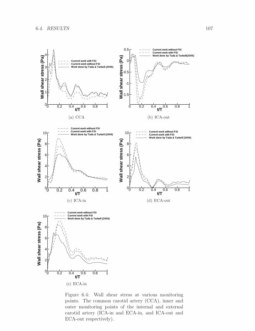
6.4. RESULTS 107
t/T
Wal
lshe
arst
ress
(Pa)
0 0.2 0.4 0.6 0.8 10
1
2
3
4
Current work with FSICurrent work without FSIWork done by Tada & Tarbell (2005)
(a) CCA
t/T
Wal
lshe
arst
ress
(Pa)
0 0.2 0.4 0.6 0.8 1
-1.5
-1
-0.5
0
0.5 Current work without FSICurrent work with FSIWork done by Tada & Tarbell(2005)
(b) ICA-out
t/T
Wal
lshe
arst
ress
(Pa)
0 0.2 0.4 0.6 0.8 10
2
4
6
8
10Current work without FSICurrent work with FSIWork done by Tada & Tarbell (2005)
(c) ICA-in
t/T
Wal
lshe
arst
ress
(Pa)
0 0.2 0.4 0.6 0.8 10
2
4
6
8
10 Current work without FSICurrent work with FSIWork done by Tada & Tarbell (2005)
(d) ECA-out
t/T
Wal
lshe
arst
ress
(Pa)
0 0.2 0.4 0.6 0.8 10
2
4
6
8
10Current work without FSICurrent work with FSIWork done by Tada & Tarbell (2005)
(e) ECA-in
Figure 6.4: Wall shear stress at various monitoringpoints. The common carotid artery (CCA), inner andouter monitoring points of the internal and externalcarotid artery (ICA-in and ECA-in, and ICA-out andECA-out respectively).
108CHAPTER 6. FLUID-STRUCTURE INTERACTION IN CAROTID BIFURCATION
shear strain rate are extremely small when compared to those at the inner wall of
the section. For 50 percent blockage case, the flow pattern changes drastically as
demonstrated in Figure 6.5. The recirculation zone in these two cases only occurs
at the proximal and distal ends of the stenosis. Flow near the apex of the stenosis
and inner wall of the sinus is not reversed. The velocity magnitude and shear strain
rate depends strongly on the degree of stenosis.
Deformation
Figure 6.6 illustrates the region of high deformation in the carotid bifurcation. There
are two regions which have relatively high deformation when compared to other
regions in the model. These two regions are at the stenosis and upstream to the
flow divider. It can be observed that the deformation pattern does not change with
the degree of stenosis. However, the magnitude of the deformations in each region
changes with time and has variation that corresponds to the pressure waveform (see
section 4). Moreover, it also appears that as the degree of stenosis increases, the
wall deformation in the stenotic region reduces. In contrast, the deformation in the
region near the downstream of the bifurcation point seems to be insensitive to the
variation of blockage.
Maximum principal stress
Magnitude of MPS Figure 6.7 shows the region of negative MPS (compression)
that can be identified as being on the stenosis while other parts of the bifurcation
are under the condition of positive MPS (tension). Only the stenotic region is under
compression, while the rest of the artery is under tension. Moreover, as the degree of
stenosis is increased, the magnitude of the negative MPS may get larger as illustrated
in Figure 6.9. In the case with 10 percent blockage, the region of negative MPS is
located in a very confined region on the apex of the stenosis. The negative MPS
region tends to expand as the degree of stenosis increases.
6.4. RESULTS 109
(a) 0 percent blockage (healthy case) (b) 10 percent blockage
(c) 25 percent blockage (d) 50 percent blockage
Figure 6.5: Flow pattern in carotid bifurcation with dif-ferent degrees of stenosis.
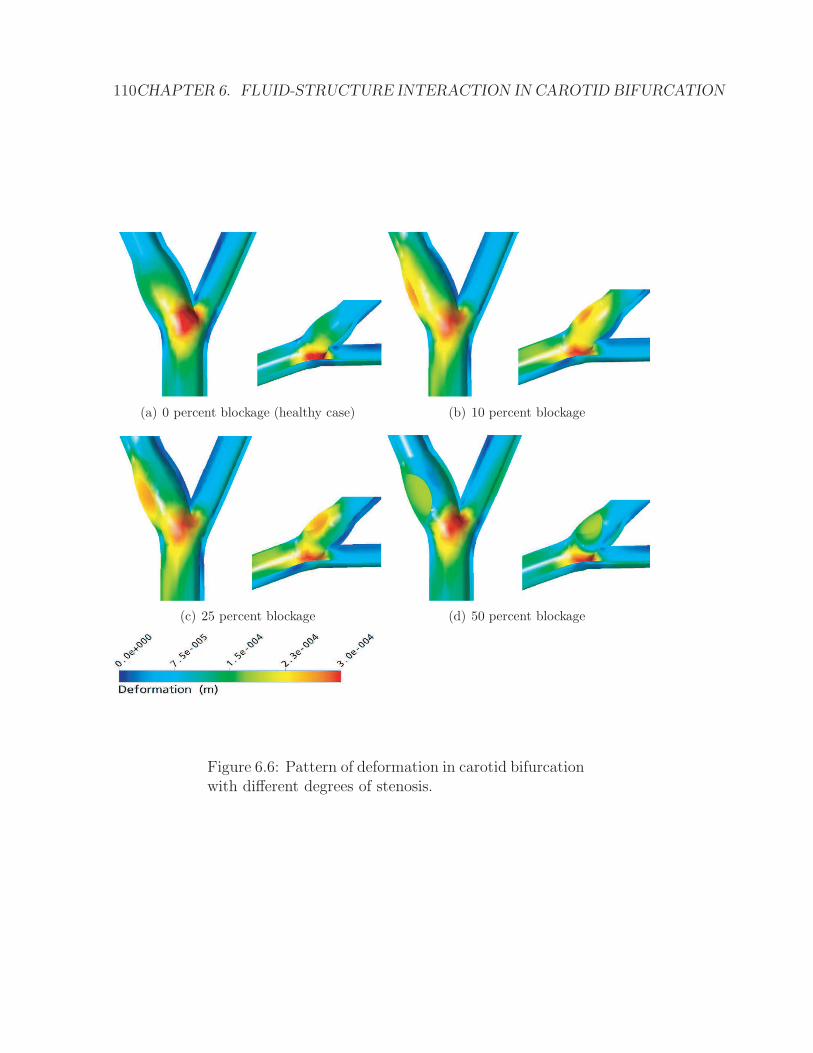
110CHAPTER 6. FLUID-STRUCTURE INTERACTION IN CAROTID BIFURCATION
(a) 0 percent blockage (healthy case)
(b) 10 percent blockage
(c) 25 percent blockage
(d) 50 percent blockage
Figure 6.6: Pattern of deformation in carotid bifurcationwith different degrees of stenosis.
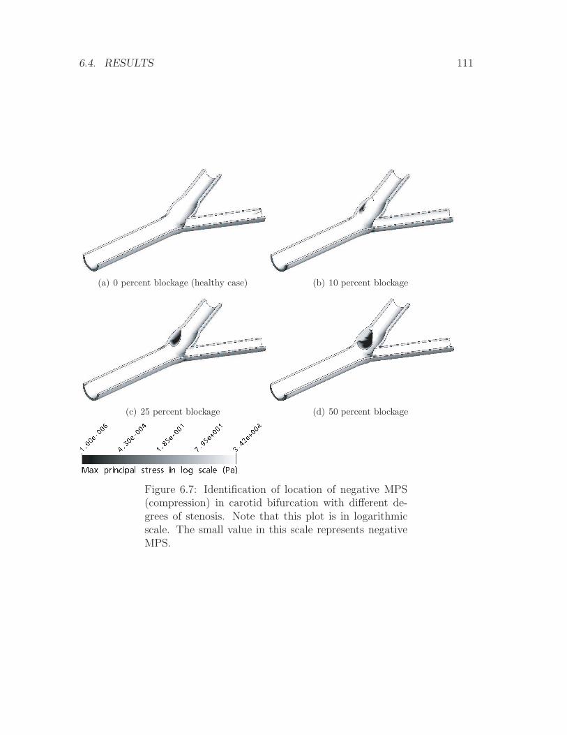
6.4. RESULTS 111
(a) 0 percent blockage (healthy case) (b) 10 percent blockage
(c) 25 percent blockage (d) 50 percent blockage
Figure 6.7: Identification of location of negative MPS(compression) in carotid bifurcation with different de-grees of stenosis. Note that this plot is in logarithmicscale. The small value in this scale represents negativeMPS.
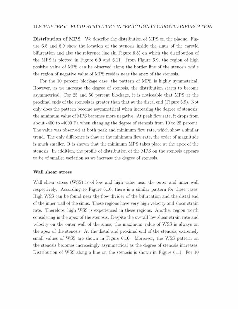
112CHAPTER 6. FLUID-STRUCTURE INTERACTION IN CAROTID BIFURCATION
Distribution of MPS We describe the distribution of MPS on the plaque. Fig-
ure 6.8 and 6.9 show the location of the stenosis inside the sinus of the carotid
bifurcation and also the reference line (in Figure 6.8) on which the distribution of
the MPS is plotted in Figure 6.9 and 6.11. From Figure 6.9, the region of high
positive value of MPS can be observed along the border line of the stenosis while
the region of negative value of MPS resides near the apex of the stenosis.
For the 10 percent blockage case, the pattern of MPS is highly symmetrical.
However, as we increase the degree of stenosis, the distribution starts to become
asymmetrical. For 25 and 50 percent blockage, it is noticeable that MPS at the
proximal ends of the stenosis is greater than that at the distal end (Figure 6.9). Not
only does the pattern become asymmetrical when increasing the degree of stenosis,
the minimum value of MPS becomes more negative. At peak flow rate, it drops from
about -400 to -4000 Pa when changing the degree of stenosis from 10 to 25 percent.
The value was observed at both peak and minimum flow rate, which show a similar
trend. The only difference is that at the minimum flow rate, the order of magnitude
is much smaller. It is shown that the minimum MPS takes place at the apex of the
stenosis. In addition, the profile of distribution of the MPS on the stenosis appears
to be of smaller variation as we increase the degree of stenosis.
Wall shear stress
Wall shear stress (WSS) is of low and high value near the outer and inner wall
respectively. According to Figure 6.10, there is a similar pattern for these cases.
High WSS can be found near the flow divider of the bifurcation and the distal end
of the inner wall of the sinus. These regions have very high velocity and shear strain
rate. Therefore, high WSS is experienced in these regions. Another region worth
considering is the apex of the stenosis. Despite the overall low shear strain rate and
velocity on the outer wall of the sinus, the maximum value of WSS is always on
the apex of the stenosis. At the distal and proximal end of the stenosis, extremely
small values of WSS are shown in Figure 6.10. Moreover, the WSS pattern on
the stenosis becomes increasingly asymmetrical as the degree of stenosis increases.
Distribution of WSS along a line on the stenosis is shown in Figure 6.11. For 10
6.4. RESULTS 113
(a) 10 percent blockage (b) 25 percent blockage
(c) 50 percent blockage
Figure 6.8: Contours of MPS distributions based on dif-ferent degrees of stenosis.
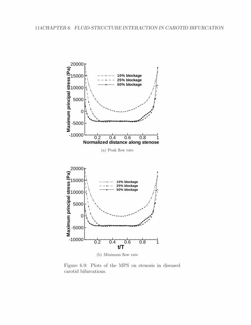
114CHAPTER 6. FLUID-STRUCTURE INTERACTION IN CAROTID BIFURCATION
Normalized distance along stenose
Max
imum
prin
cipa
lstre
ss(P
a)
0.2 0.4 0.6 0.8 1-10000
-5000
0
5000
10000
15000
20000
10% blockage25% blockage50% blockage
(a) Peak flow rate
t/T
Max
imum
prin
cipa
lstre
ss(P
a)
0.2 0.4 0.6 0.8 1-10000
-5000
0
5000
10000
15000
20000
10% blockage25% blockage50% blockage
(b) Minimum flow rate
Figure 6.9: Plots of the MPS on stenosis in diseasedcarotid bifurcations.
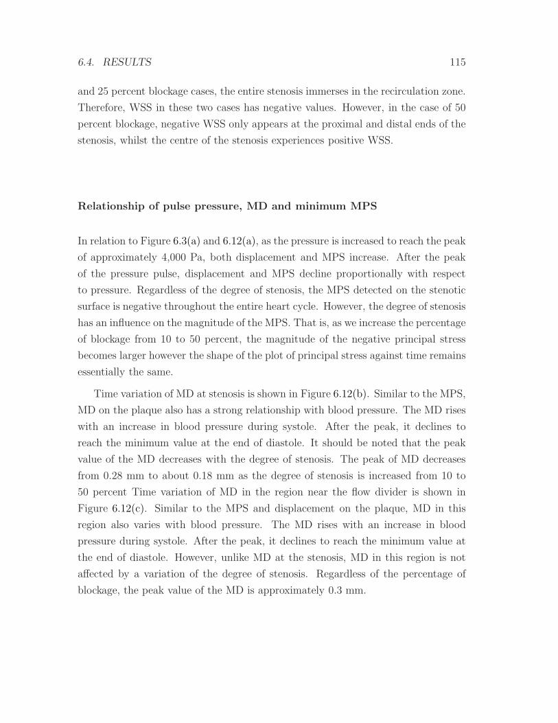
6.4. RESULTS 115
and 25 percent blockage cases, the entire stenosis immerses in the recirculation zone.
Therefore, WSS in these two cases has negative values. However, in the case of 50
percent blockage, negative WSS only appears at the proximal and distal ends of the
stenosis, whilst the centre of the stenosis experiences positive WSS.
Relationship of pulse pressure, MD and minimum MPS
In relation to Figure 6.3(a) and 6.12(a), as the pressure is increased to reach the peak
of approximately 4,000 Pa, both displacement and MPS increase. After the peak
of the pressure pulse, displacement and MPS decline proportionally with respect
to pressure. Regardless of the degree of stenosis, the MPS detected on the stenotic
surface is negative throughout the entire heart cycle. However, the degree of stenosis
has an influence on the magnitude of the MPS. That is, as we increase the percentage
of blockage from 10 to 50 percent, the magnitude of the negative principal stress
becomes larger however the shape of the plot of principal stress against time remains
essentially the same.
Time variation of MD at stenosis is shown in Figure 6.12(b). Similar to the MPS,
MD on the plaque also has a strong relationship with blood pressure. The MD rises
with an increase in blood pressure during systole. After the peak, it declines to
reach the minimum value at the end of diastole. It should be noted that the peak
value of the MD decreases with the degree of stenosis. The peak of MD decreases
from 0.28 mm to about 0.18 mm as the degree of stenosis is increased from 10 to
50 percent Time variation of MD in the region near the flow divider is shown in
Figure 6.12(c). Similar to the MPS and displacement on the plaque, MD in this
region also varies with blood pressure. The MD rises with an increase in blood
pressure during systole. After the peak, it declines to reach the minimum value at
the end of diastole. However, unlike MD at the stenosis, MD in this region is not
affected by a variation of the degree of stenosis. Regardless of the percentage of
blockage, the peak value of the MD is approximately 0.3 mm.
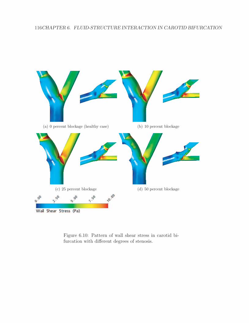
116CHAPTER 6. FLUID-STRUCTURE INTERACTION IN CAROTID BIFURCATION
(a) 0 percent blockage (healthy case)
(b) 10 percent blockage
(c) 25 percent blockage
(d) 50 percent blockage
Figure 6.10: Pattern of wall shear stress in carotid bi-furcation with different degrees of stenosis.
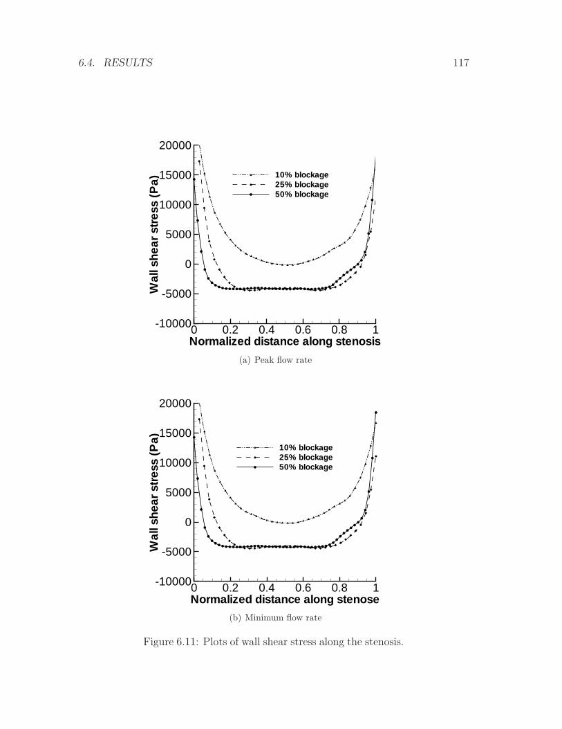
6.4. RESULTS 117
Normalized distance along stenosis
Wal
lshe
arst
ress
(Pa)
0 0.2 0.4 0.6 0.8 1-10000
-5000
0
5000
10000
15000
20000
10% blockage25% blockage50% blockage
(a) Peak flow rate
Normalized distance along stenose
Wal
lshe
arst
ress
(Pa)
0 0.2 0.4 0.6 0.8 1-10000
-5000
0
5000
10000
15000
20000
10% blockage25% blockage50% blockage
(b) Minimum flow rate
Figure 6.11: Plots of wall shear stress along the stenosis.
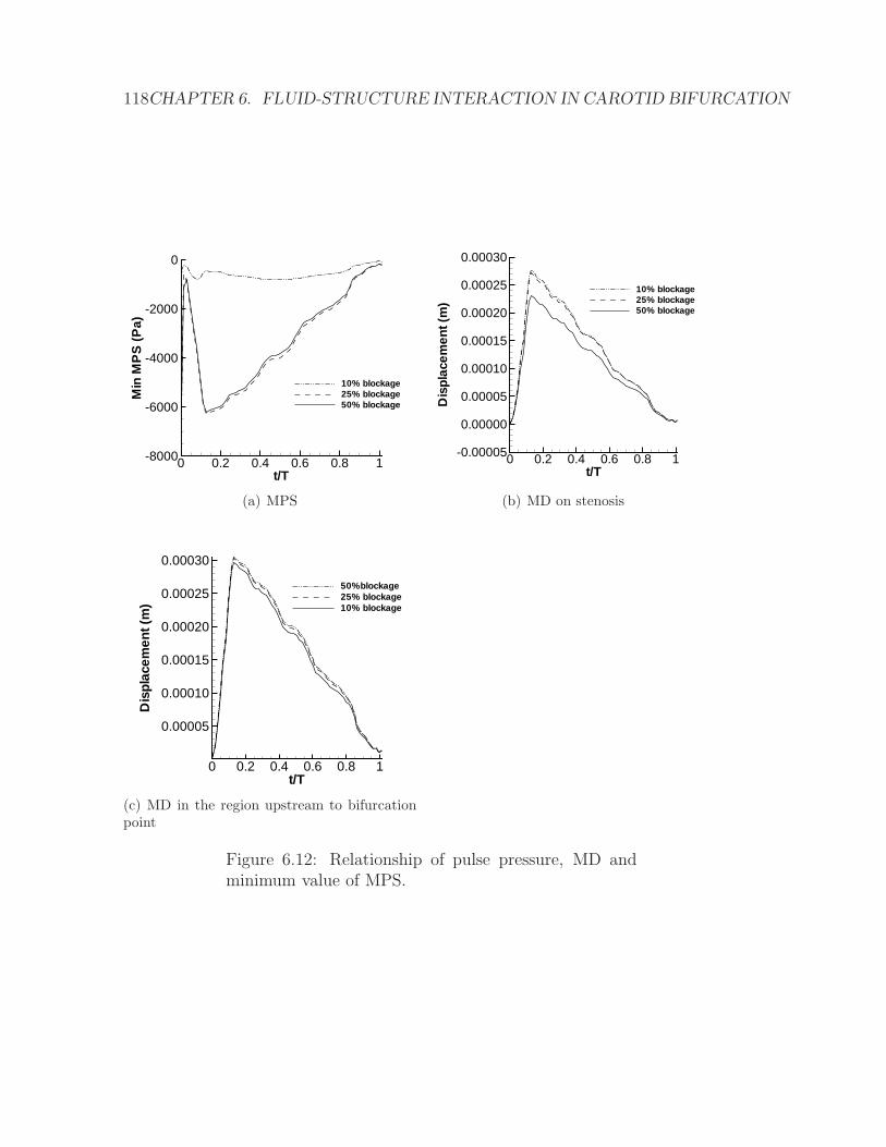
118CHAPTER 6. FLUID-STRUCTURE INTERACTION IN CAROTID BIFURCATION
t/T
Min
MP
S(P
a)
0 0.2 0.4 0.6 0.8 1-8000
-6000
-4000
-2000
0
10% blockage25% blockage50% blockage
(a) MPS
t/T
Dis
plac
emen
t(m
)0 0.2 0.4 0.6 0.8 1-0.00005
0.00000
0.00005
0.00010
0.00015
0.00020
0.00025
0.00030
10% blockage25% blockage50% blockage
(b) MD on stenosis
t/T
Dis
plac
emen
t(m
)
0 0.2 0.4 0.6 0.8 1
0.00005
0.00010
0.00015
0.00020
0.00025
0.00030
50%blockage25% blockage10% blockage
(c) MD in the region upstream to bifurcationpoint
Figure 6.12: Relationship of pulse pressure, MD andminimum value of MPS.
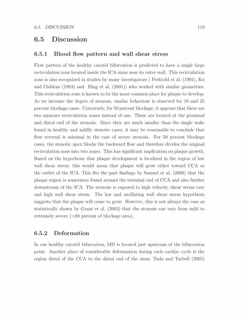
6.5. DISCUSSION 119
6.5 Discussion
6.5.1 Blood flow pattern and wall shear stress
Flow pattern of the healthy carotid bifurcation is predicted to have a single large
recirculation zone located inside the ICA sinus near its outer wall. This recirculation
zone is also recognized in studies by many investigators ( Perktold et al. (1991), Ku
and Giddens (1983) and Ding et al. (2001)) who worked with similar geometries.
This recirculation zone is known to be the most common place for plaque to develop.
As we increase the degree of stenosis, similar behaviour is observed for 10 and 25
percent blockage cases. Conversely, for 50 percent blockage, it appears that there are
two separate recirculation zones instead of one. These are located at the proximal
and distal end of the stenosis. Since they are much smaller than the single wake
found in healthy and mildly stenotic cases, it may be reasonable to conclude that
flow reversal is minimal in the case of severe stenosis. For 50 percent blockage
cases, the stenotic apex blocks the backward flow and therefore divides the original
recirculation zone into two zones. This has significant implication on plaque growth.
Based on the hypothesis that plaque development is localized in the region of low
wall shear stress, this would mean that plaque will grow either toward CCA or
the outlet of the ICA. This fits the past findings by Samuel et al. (2008) that the
plaque region is sometimes found around the terminal end of CCA and also further
downstream of the ICA. The stenosis is exposed to high velocity, shear strain rate
and high wall shear stress. The low and oscillating wall shear stress hypothesis
suggests that the plaque will cease to grow. However, this is not always the case as
statistically shown by Grant et al. (2003) that the stenosis can vary from mild to
extremely severe (>80 percent of blockage area).
6.5.2 Deformation
In our healthy carotid bifurcation, MD is located just upstream of the bifurcation
point. Another place of considerable deformation during each cardiac cycle is the
region distal of the CCA to the distal end of the sinus. Tada and Tarbell (2005)
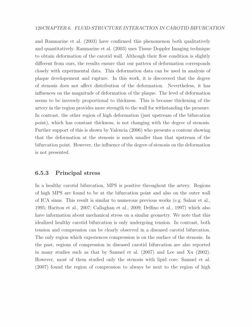
120CHAPTER 6. FLUID-STRUCTURE INTERACTION IN CAROTID BIFURCATION
and Ramnarine et al. (2003) have confirmed this phenomenon both qualitatively
and quantitatively. Ramnarine et al. (2003) uses Tissue Doppler Imaging technique
to obtain deformation of the carotid wall. Although their flow condition is slightly
different from ours, the results ensure that our pattern of deformation corresponds
closely with experimental data. This deformation data can be used in analysis of
plaque developement and rupture. In this work, it is discovered that the degree
of stenosis does not affect distribution of the deformation. Nevertheless, it has
influences on the magnitude of deformation of the plaque. The level of deformation
seems to be inversely proportional to thickness. This is because thickening of the
artery in the region provides more strength to the wall for withstanding the pressure.
In contrast, the other region of high deformation (just upstream of the bifurcation
point), which has constant thickness, is not changing with the degree of stenosis.
Further support of this is shown by Valencia (2006) who presents a contour showing
that the deformation at the stenosis is much smaller than that upstream of the
bifurcation point. However, the influence of the degree of stenosis on the deformation
is not presented.
6.5.3 Principal stress
In a healthy carotid bifurcation, MPS is positive throughout the artery. Regions
of high MPS are found to be at the bifurcation point and also on the outer wall
of ICA sinus. This result is similar to numerous previous works (e.g. Salzar et al.,
1995; Hariton et al., 2007; Callaghan et al., 2009; Delfino et al., 1997) which also
have information about mechanical stress on a similar geometry. We note that this
idealized healthy carotid bifurcation is only undergoing tension. In contrast, both
tension and compression can be clearly observed in a diseased carotid bifurcation.
The only region which experiences compression is on the surface of the stenosis. In
the past, regions of compression in diseased carotid bifurcation are also reported
in many studies such as that by Samuel et al. (2007) and Lee and Xu (2002).
However, most of them studied only the stenosis with lipid core. Samuel et al.
(2007) found the region of compression to always be next to the region of high
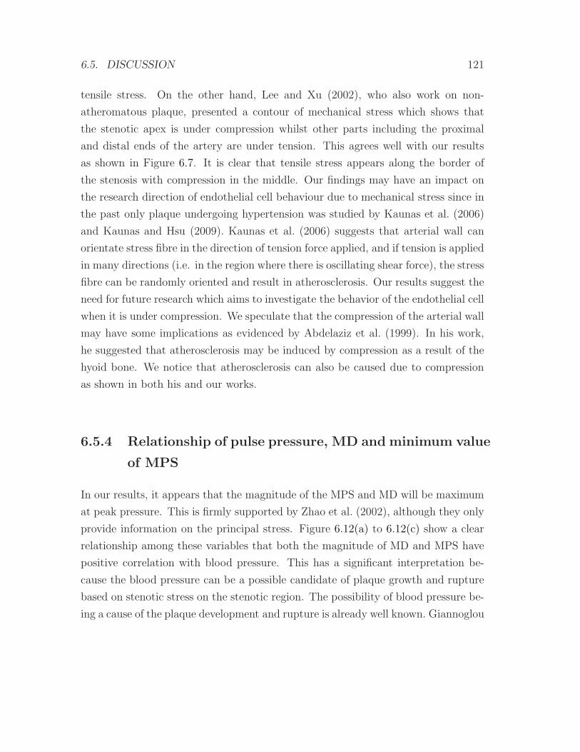
6.5. DISCUSSION 121
tensile stress. On the other hand, Lee and Xu (2002), who also work on non-
atheromatous plaque, presented a contour of mechanical stress which shows that
the stenotic apex is under compression whilst other parts including the proximal
and distal ends of the artery are under tension. This agrees well with our results
as shown in Figure 6.7. It is clear that tensile stress appears along the border of
the stenosis with compression in the middle. Our findings may have an impact on
the research direction of endothelial cell behaviour due to mechanical stress since in
the past only plaque undergoing hypertension was studied by Kaunas et al. (2006)
and Kaunas and Hsu (2009). Kaunas et al. (2006) suggests that arterial wall can
orientate stress fibre in the direction of tension force applied, and if tension is applied
in many directions (i.e. in the region where there is oscillating shear force), the stress
fibre can be randomly oriented and result in atherosclerosis. Our results suggest the
need for future research which aims to investigate the behavior of the endothelial cell
when it is under compression. We speculate that the compression of the arterial wall
may have some implications as evidenced by Abdelaziz et al. (1999). In his work,
he suggested that atherosclerosis may be induced by compression as a result of the
hyoid bone. We notice that atherosclerosis can also be caused due to compression
as shown in both his and our works.
6.5.4 Relationship of pulse pressure, MD and minimum value
of MPS
In our results, it appears that the magnitude of the MPS and MD will be maximum
at peak pressure. This is firmly supported by Zhao et al. (2002), although they only
provide information on the principal stress. Figure 6.12(a) to 6.12(c) show a clear
relationship among these variables that both the magnitude of MD and MPS have
positive correlation with blood pressure. This has a significant interpretation be-
cause the blood pressure can be a possible candidate of plaque growth and rupture
based on stenotic stress on the stenotic region. The possibility of blood pressure be-
ing a cause of the plaque development and rupture is already well known. Giannoglou
122CHAPTER 6. FLUID-STRUCTURE INTERACTION IN CAROTID BIFURCATION
et al. (2008) speculates that the elevated heart rate that leads to an increase in ex-
posure time of high blood pressure, and can well be an indicator of atherosclerotic
risk. In our work, it is revealed that the plaque undergoes extremely high and low
compression during systole and diastole. Therefore, an elevated heart rate can place
the artery in a condition whereby it has to withstand the high compressive force for
long periods of time.
6.6 Summary and concluding remarks
We summarize that different degrees of stenosis have a significant influence on three
basic characteristics of atherosclerosis. Firstly, the presence of severe stenosis can
dramatically alter the blood flow pattern. Flow reversal is found to be smaller at
advanced stages of the disease. This leads to diminishing low WSS in the stenotic
region. Secondly, the apex of stenosis experiences compressive stress which can
intensify as it grows. This explains why plaque can still grow at advanced stages
when the wall shear stress is higher. Finally, the relationship among pulse pressure,
MD and MPS suggests that elevated heart rate can lead to a higher risk of stroke
due to longer exposure to high MD and MPS. However, determining a proper range
of suitable heart rate is beyond the scope of this current work.
Chapter 7
Concluding Remarks
7.1 Achievements and their significances
The achievements made in this work are summarized as follows.
7.1.1 Numerical and theoretical analysis on influence of struc-
tural time integration schemes on added mass insta-
bility in FSI
We have shown that stability condition of FSI calculation can be influenced signifi-
cantly and allows a higher relaxation factor to be used. This means that computa-
tional cost can be greatly reduced by selecting a proper structural time integration
scheme. However, the performance depends largely on the following factors:
• Applied numerical damping;
• Density ratio;
• Time step size;
• Geometrical properties such as radius and thickness of vessel.
123
124 CHAPTER 7. CONCLUDING REMARKS
The critical relaxation factor is higher when using the structural time integration
scheme that does not contain any numerical damping (γ = 0). On the other hand,
the choice of time integration schemes for discretizing fluid acceleration also has a
strong impact on the stability condition. Our results suggest that more accurate
schemes such as the second order accurate backward Euler leads to a more difficult
condition for stability of FSI. Another important parameter is time step size used
for computation. In particular, smaller time step size results in a more restrictive
condition. However, as the time step size approaches zero, the value of the critical
relaxation factor converges to a specific value. Another factor worth considering is
the density ratio. It is found that this value has a considerable impact on FSI per-
formance. In particular, the stability condition becomes invariant with the choice
of structural time integration schemes in cases of high density ratio, while in the
cases of low density ratio, this value depends largely on the schemes used. Finally,
the condition is more restrictive when radius of the flexible vessel is greater due
to an increase in maximum eigenvalue of the added mass operator. Moreover, the
developement of artificial compressibility can be used to further improve FSI perfor-
mance. It is found that this method can handle added mass instability efficiently and
its performance does not depend on the following critical parameters listed above.
7.1.2 Performance comparision between under-relaxation tech-
nique and artificial compressibility
The performance of FSI using under-relaxation technique is compared to that using
artificial compressibility by considering the amount of computational time required
at various density ratio. Although, at low density ratio, the performance of under-
relaxation technique appears to be slightly better than that of artificial compress-
ibility, it is found that artificial compressibility is more efficient when density ratio
is high. Therefore, it is concluded that artificial compressibility is a more applicable
tools for dealing with a wide range of engineering applications whereby high density
ratio is an unavoidable property.
7.2. FUTURE WORK 125
7.1.3 Application of artificial compressibility to artheroscle-
rosis in carotid bifurcation
Apart from being used as a demonstration of practicality of artificial compressibility
for solving high density ratio problems, the analysis of artherosclerosis in carotid
bifurcation using FSI also provides considerable input to this research field. The
analysis serves the biomedical engineering research community in many aspects.
The contributions from analysing this application can be summarized below.
• An insight on the influence of the degree of stenosis on mechanical stress
experienced in carotid bifurcation. This provides an alternative explanation
of how the stenotic plaque grows at the advanced stage of the disease. From
the results in Chapter 6, the high level of mechanical stress is observed and
can be the reason behind the growth of stenosis when the low and oscillating
wall shear stress region disappears.
• An understanding of how blood flow pattern changes with the presence of
stenosis with different sizes. It gives useful information about flow pattern
inside carotid bifurcation at different degree of stenosis. Flow behavior dra-
matically changes as we increase the degree of blockage. This can be used as a
future reference for other investigators in this field of biomedical engineering.
• A relationship between blood pressure, structural stress and deformation of
the stenotic plaque. It establishes a firm relationship between flow pressure
and mechanical stress which can be useful for determining a proper range of
blood pressure in patients.
7.2 Future Work
In this work, only the generalized-α structural time integration schemes are
used for the stability analysis. In the future, it may be useful to conduct a
126 CHAPTER 7. CONCLUDING REMARKS
similar study with other advanced time integration schemes such as Runge-
Kutta schemes. Further analysis with other advanced schemes will provide
more complete information of how the instability behaves. Moreover, it will
provide guidelines to a wider range of researchers for conducting FSI problems
of their interest because FSI codes use different schemes.
Artificial compressibility can be utilized efficiently for various engineering ap-
plications, and especially those involving internal incompressible flows. How-
ever, this method may not be applicable to problems in the following cate-
gories:
– External flow;
– Compressible flow.
These are potential areas which need improvements. For example, in com-
pressible flow, the artificial compressiblity term, which is introduced to the
fluid solver, may take a large number of coupling steps in order to vanish and
not affect the real flow solution.
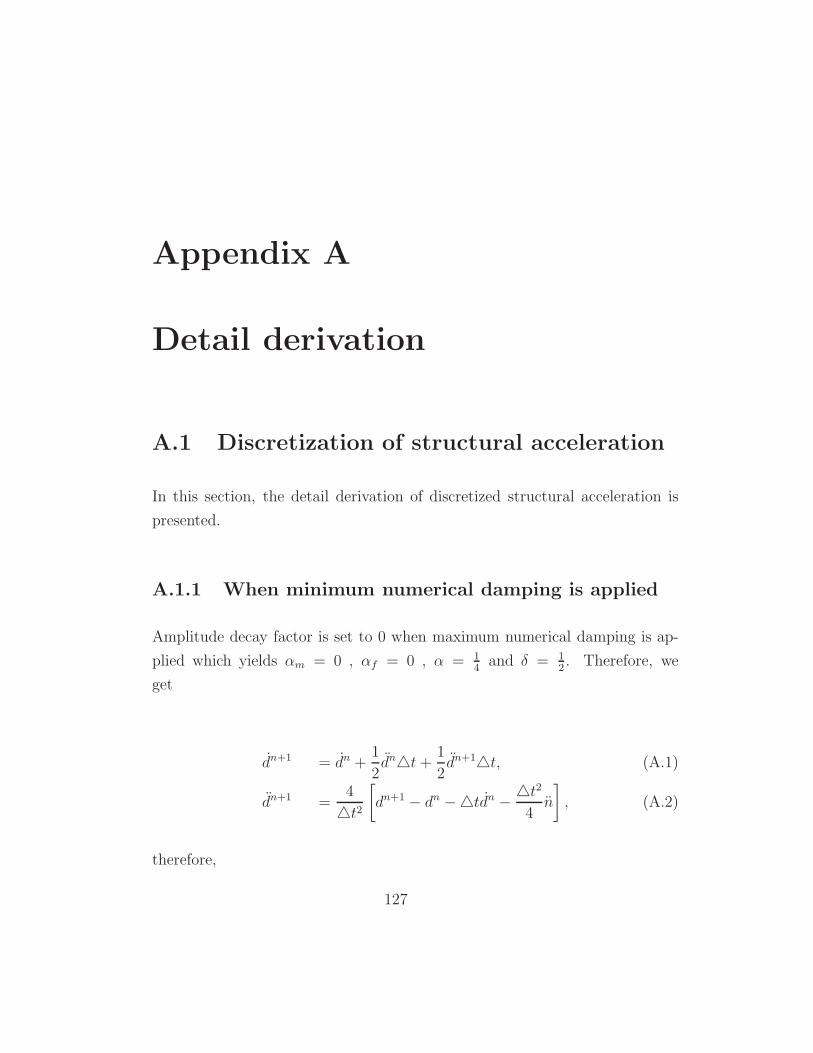
Appendix A
Detail derivation
A.1 Discretization of structural acceleration
In this section, the detail derivation of discretized structural acceleration is
presented.
A.1.1 When minimum numerical damping is applied
Amplitude decay factor is set to 0 when maximum numerical damping is ap-
plied which yields αm = 0 , αf = 0 , α = 14and δ = 1
2. Therefore, we
get
dn+1 = dn +1
2dn4t+
1
2dn+14t, (A.1)
dn+1 =4
4t2
[dn+1 − dn −4tdn − 4t2
4n
], (A.2)
therefore,
127
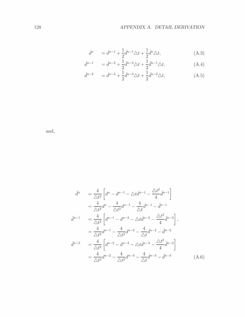
128 APPENDIX A. DETAIL DERIVATION
dn = dn−1 +1
2dn−14t+
1
2dn4t, (A.3)
dn−1 = dn−2 +1
2dn−24t+
1
2dn−14t, (A.4)
dn−2 = dn−3 +1
2dn−34t+
1
2dn−24t, (A.5)
and,
dn =4
4t2
[dn − dn−1 −4tdn−1 − 4t2
4dn−1
]
=4
4t2dn − 4
4t2dn−1 − 4
4tdn−1 − dn−1
dn−1 =4
4t2
[dn−1 − dn−2 −4tdn−2 − 4t2
4dn−2
],
=4
4t2dn−1 − 4
4t2dn−2 − 4
4tdn−2 − dn−2
dn−2 =4
4t2
[dn−2 − dn−3 −4tdn−3 − 4t2
4dn−3
]
=4
4t2dn−2 − 4
4t2dn−3 − 4
4tdn−3 − dn−3 (A.6)
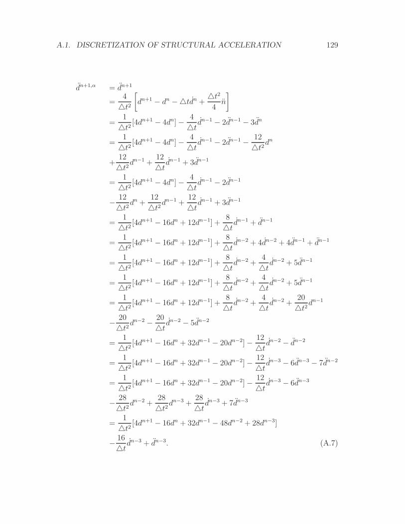
A.1. DISCRETIZATION OF STRUCTURAL ACCELERATION 129
dn+1,α = dn+1
=4
4t2
[dn+1 − dn −4tdn +
4t2
4n
]
=1
4t2[4dn+1 − 4dn]− 4
4tdn−1 − 2dn−1 − 3dn
=1
4t2[4dn+1 − 4dn]− 4
4tdn−1 − 2dn−1 − 12
4t2dn
+12
4t2dn−1 +
12
4tdn−1 + 3dn−1
=1
4t2[4dn+1 − 4dn]− 4
4tdn−1 − 2dn−1
− 12
4t2dn +
12
4t2dn−1 +
12
4tdn−1 + 3dn−1
=1
4t2[4dn+1 − 16dn + 12dn−1] +
8
4tdn−1 + dn−1
=1
4t2[4dn+1 − 16dn + 12dn−1] +
8
4tdn−2 + 4dn−2 + 4dn−1 + dn−1
=1
4t2[4dn+1 − 16dn + 12dn−1] +
8
4tdn−2 +
4
4tdn−2 + 5dn−1
=1
4t2[4dn+1 − 16dn + 12dn−1] +
8
4tdn−2 +
4
4tdn−2 + 5dn−1
=1
4t2[4dn+1 − 16dn + 12dn−1] +
8
4tdn−2 +
4
4tdn−2 +
20
4t2dn−1
− 20
4t2dn−2 − 20
4tdn−2 − 5dn−2
=1
4t2[4dn+1 − 16dn + 32dn−1 − 20dn−2]− 12
4tdn−2 − dn−2
=1
4t2[4dn+1 − 16dn + 32dn−1 − 20dn−2]− 12
4tdn−3 − 6dn−3 − 7dn−2
=1
4t2[4dn+1 − 16dn + 32dn−1 − 20dn−2]− 12
4tdn−3 − 6dn−3
− 28
4t2dn−2 +
28
4t2dn−3 +
28
4tdn−3 + 7dn−3
=1
4t2[4dn+1 − 16dn + 32dn−1 − 48dn−2 + 28dn−3]
− 16
4tdn−3 + dn−3. (A.7)
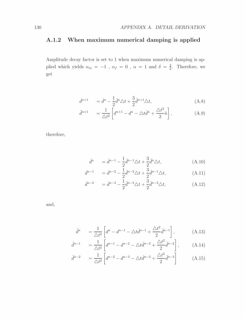
130 APPENDIX A. DETAIL DERIVATION
A.1.2 When maximum numerical damping is applied
Amplitude decay factor is set to 1 when maximum numerical damping is ap-
plied which yields αm = −1 , αf = 0 , α = 1 and δ = 32. Therefore, we
get
dn+1 = dn − 1
2dn4t+
3
2dn+14t, (A.8)
dn+1 =1
4t2
[dn+1 − dn −4tdn +
4t2
2n
], (A.9)
therefore,
dn = dn−1 − 1
2dn−14t+
3
2dn4t, (A.10)
dn−1 = dn−2 − 1
2dn−24t+
3
2dn−14t, (A.11)
dn−2 = dn−3 − 1
2dn−34t+
3
2dn−24t, (A.12)
and,
dn =1
4t2
[dn − dn−1 −4tdn−1 +
4t2
2dn−1
], (A.13)
dn−1 =1
4t2
[dn−1 − dn−2 −4tdn−2 +
4t2
2dn−2
], (A.14)
dn−2 =1
4t2
[dn−2 − dn−3 −4tdn−3 +
4t2
2dn−3
](A.15)
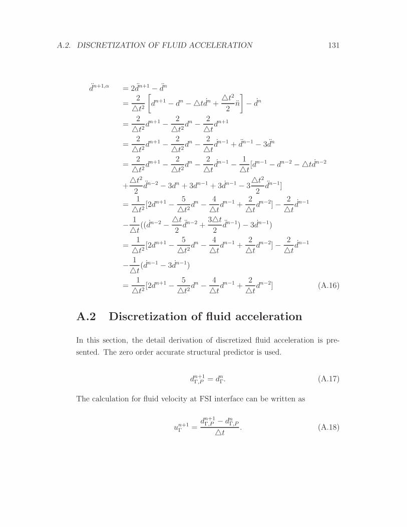
A.2. DISCRETIZATION OF FLUID ACCELERATION 131
dn+1,α = 2dn+1 − dn
=2
4t2
[dn+1 − dn −4tdn +
4t2
2n
]− dn
=2
4t2dn+1 − 2
4t2dn − 2
4tdn+1
=2
4t2dn+1 − 2
4t2dn − 2
4tdn−1 + dn−1 − 3dn
=2
4t2dn+1 − 2
4t2dn − 2
4tdn−1 − 1
4t[dn−1 − dn−2 −4tdn−2
+4t2
2dn−2 − 3dn + 3dn−1 + 3dn−1 − 3
4t2
2dn−1]
=1
4t2[2dn+1 − 5
4t2dn − 4
4tdn−1 +
2
4tdn−2]− 2
4tdn−1
− 1
4t((dn−2 − 4t
2dn−2 +
34t
2dn−1)− 3dn−1)
=1
4t2[2dn+1 − 5
4t2dn − 4
4tdn−1 +
2
4tdn−2]− 2
4tdn−1
− 1
4t(dn−1 − 3dn−1)
=1
4t2[2dn+1 − 5
4t2dn − 4
4tdn−1 +
2
4tdn−2] (A.16)
A.2 Discretization of fluid acceleration
In this section, the detail derivation of discretized fluid acceleration is pre-
sented. The zero order accurate structural predictor is used.
dn+1Γ,P = dnΓ. (A.17)
The calculation for fluid velocity at FSI interface can be written as
un+1Γ =
dn+1Γ,P − dnΓ,P
4t. (A.18)
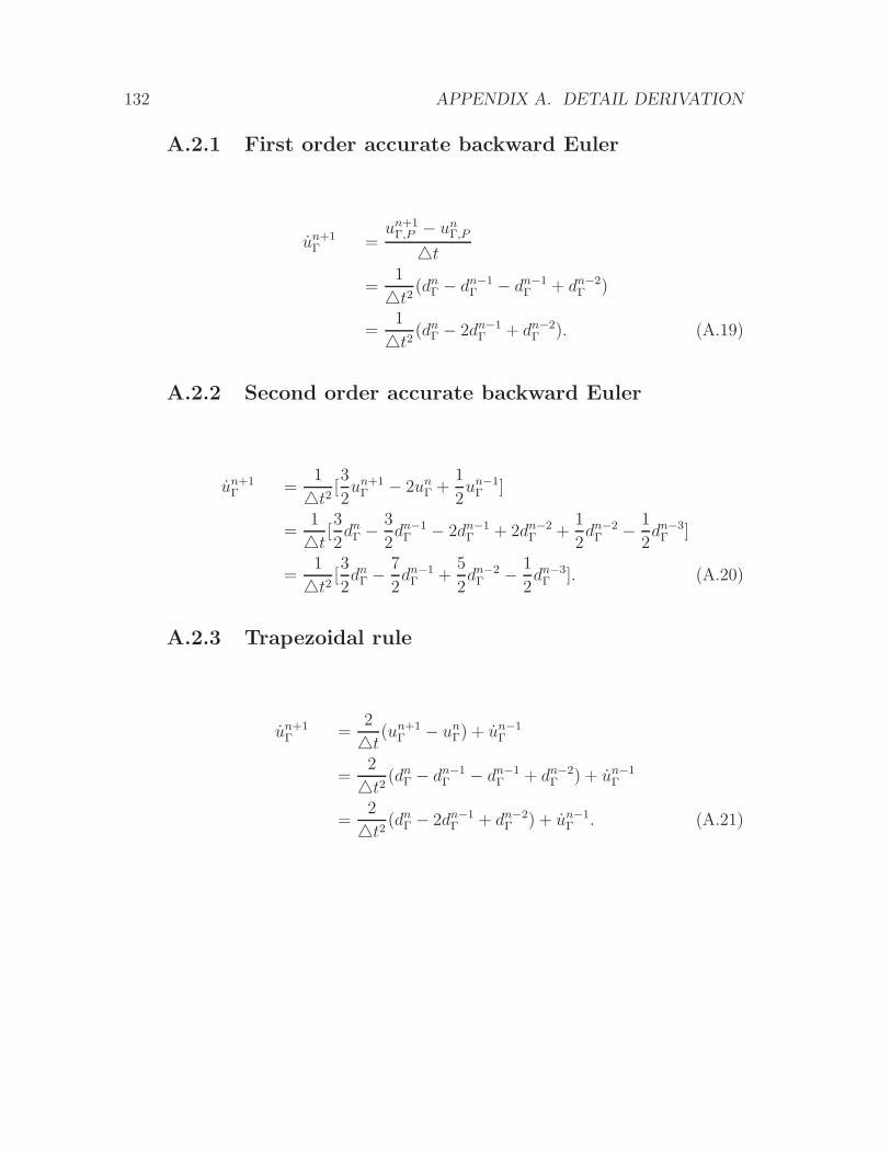
132 APPENDIX A. DETAIL DERIVATION
A.2.1 First order accurate backward Euler
un+1Γ =
un+1Γ,P − un
Γ,P
4t
=1
4t2(dnΓ − dn−1
Γ − dn−1Γ + dn−2
Γ )
=1
4t2(dnΓ − 2dn−1
Γ + dn−2Γ ). (A.19)
A.2.2 Second order accurate backward Euler
un+1Γ =
1
4t2[3
2un+1Γ − 2un
Γ +1
2un−1Γ ]
=1
4t[3
2dnΓ −
3
2dn−1Γ − 2dn−1
Γ + 2dn−2Γ +
1
2dn−2Γ − 1
2dn−3Γ ]
=1
4t2[3
2dnΓ −
7
2dn−1Γ +
5
2dn−2Γ − 1
2dn−3Γ ]. (A.20)
A.2.3 Trapezoidal rule
un+1Γ =
2
4t(un+1
Γ − unΓ) + un−1
Γ
=2
4t2(dnΓ − dn−1
Γ − dn−1Γ + dn−2
Γ ) + un−1Γ
=2
4t2(dnΓ − 2dn−1
Γ + dn−2Γ ) + un−1
Γ . (A.21)
Appendix B
Analysis on added mass
instability
In the solution procedure of fluid-structure interaction (FSI), the so-call arti-
ficial added mass effect plays an important role in determining the stability
of the computation. We propose a derivation using Von Neumann stability
analysis, which shows its significance as a tool for studying this numerical in-
stability. Our derivation demonstrates that FSI solution is severely unstable
when density ratio is high, solid structure is thin and flexible. It also shows
that this instability can be eliminated by introducing aritificial compressibility.
B.1 Analysis
In this section, the instability of fluid-structure interaction using partitioned
approach is discussed. This section is divided into two sub-sections. The first
one is the derivation of instability which occurs when using Leap-Frog and
forward Euler schemes without artificial compressibility. The second one is
the derivation of instability which occurs when using Leap-Frog and forward
Euler schemes with artificial compressibility.
133
134 APPENDIX B. ANALYSIS ON ADDED MASS INSTABILITY
B.1.1 Leap-Frog and Euler scheme with under-relaxation
We refer to the governing equation of deformation of a flexible cylindrical tube
in (Causin et al., 2005), which can be written as
ρshs
∂2dsΓ∂t2
+ ρfMa
∂2dfΓ∂t2
+ a0dsΓ − b
∂2dsΓ∂x2
= Pext,Γ, (B.1)
where a0 =Ehs
r2(1−ν2)and b = KTBhs.
The Leap-Frog scheme for structural acceleration is written as
dn+1,sΓ =
1
∆t2(dn+1
Γ − 2dnΓ + dn−1Γ ). (B.2)
The Euler scheme for FSI interface acceleration for fluid domain is written as
dn+1,fΓ = 1
∆t(dnΓ − dn−1
Γ ) = 1∆t2
(dnΓ − 2dn−1Γ + dn−2
Γ ). (B.3)
It is noted that superscript m represents pseudo time step or stagger itera-
tion, while n represents physical time step. Also, x and t are space and time
respectively.
Due to the nature of sequential approach, the information used for calcula-
tion of FSI interface acceleration for fluid domain is always one step behind
solid. From (B.1), since we are interested in added-mass instability, where the
mass term is dominated the stiffness term, we will neglect some non-linearity.
Therefore, (B.1) is reduced to equation (B.4) such that
ρshs
∂2dsΓ∂t2
+ ρfMa
∂2dfΓ∂t2
+ a0dsΓ = Pext,Γ. (B.4)
Discretization of (B.4) is achieved by substituting (B.2) and (B.3) to give
ρshs
4t2(dn+1
Γ − 2dnΓ + dn−1Γ ) +
ρfMa
4t2(dnΓ − 2dn−1
Γ + dn−2Γ ) + a0d
nΓ = P n
ext,Γ. (B.5)
B.1. ANALYSIS 135
To simplify it, let’s look at only one position on the interface. Notice that the
added-mass operator MA can be represented by the ith eigenvalues of MA, µi.
This make (B.5) reduced further to (B.6) as given by
ρshs
4t2(dn+1
i − 2dni + dn−1i ) +
ρfµi
4t2(dni − 2dn−1
i + dn−2i ) + a0d
ni = P n
ext,i. (B.6)
Next we will use the idea of Von Neumann stability analysis to prove stability
of the system of discrete equation (Strang, 2007). This technique based on
understanding in fourier analysis that any function can be represented by a
superposition of basis functions like sine, cosine and exponential functions.
The idea is to represent the solution in terms of initial value eiateikx, which
depends only on spatial variation x. In other words, we are trying to separate
variables x and t in our solution. This will allow us to monitor how the solution
is growing with time. Initial value of solution can be written as
d(x, t) ≈∫
∞
−∞
eiateikxdk
or
d(x, t) ≈∞∑
−∞
eiateikx. (B.7)
Note that a is a temporal wave frequency, which is also a function of spatial
wave frequency, k. For simplicity, we drop the summation sign in equation
(B.7) since our aim is to prove the instability, which can be done by monitoring
only one mode of the solution. Therefore (B.7) becomes
d(x, t) ≈ eiateikx. (B.8)
136 APPENDIX B. ANALYSIS ON ADDED MASS INSTABILITY
Now we have separated the time and space variation in our solution. From
(B.8), the initial solution is in the form of multiplication of complex exponen-
tial terms and our initial value eiateikx. The next step is to represent the other
terms (dni , dn−1i ) in term of the initial value of the system (dn−2
i ). This is set
to be the initial value because in the discrete equation (B.6), dn−2i is the oldest
information available.
Let dn−2i ≈ eiateikx, which is our initial value. Therefore, displacement at time
step n− 1 and n can be represented as
dn−1i = eia(t+∆t)eikx and dni = eia(t+2∆t)eikx.
By substituting (B.9) into (B.6), we get
ρshs
4t2(dn+1
i − 2 eia(t+2∆t)eikx + eia(t+∆t)eikx) +ρfµi
4t2(eia(t+2∆t)
−2eia(t+∆t)eikx + eikx) + a0 eia(t+2∆t)eikx = P n
ext,i. (B.9)
The growth factor is determined by rearranging above equation as
dn+1i =
{4t2
ρshs
[P next,i
eiateikx− a0e
ia2∆t − ρfµi
4t2(eia2∆t − 2eia∆t + 1
)]+ 2eia2∆t − eia∆t
}eiateikx
=
{−ρfµi
ρshs
(eia2∆t − 2eia∆t + 1
)+ 2eia2∆t − eia∆t
}eiateikx ∵ 4t2 → 0
=
{−ρfµi
ρshs
eia2∆t + 2ρfµi
ρshs
eia∆t − ρfµi
ρshs
+ 2eia2∆t − eia∆t
}eiateikx
=
{[−ρfµi
ρshs
+ 2
]eia2∆t +
[2ρfµi
ρshs
− 1
]eia∆t − ρfµi
ρshs
}
︸ ︷︷ ︸GrowthFactor
eiateikx︸ ︷︷ ︸Initial value
. (B.10)
B.1. ANALYSIS 137
The solution is unstable if the absolute value of growth factor is greater than
1. Therefore, instability occurs if (B.11) that is given as
∣∣∣∣[−ρfµi
ρshs
+ 2
]eia2∆t +
[2ρfµi
ρshs
− 1
]eia∆t − ρfµi
ρshs
∣∣∣∣ > 1 (B.11)
is satisfied.
Although the growth factor we have here is an accumulated growth over three
time step, it gives us enough information for determining if the solution of
considered system is stable or not. This is because if growth factor after three
time steps and the corresponding growth factor after one time step will still re-
sult in the same condition. A graphical representation of (B.11) can be plotted
in a complex plane and compared with a unit circle in order to demonstrate
the instability of the current scheme used for FSI as illustrated in Figures B.1.
The origin of a circle related to this growth factor is shifted by −ρfµi
ρshsin the
real axis of the complex plane. The radius is∣∣∣[−ρfµi
ρshs+ 2]+[2ρfµi
ρshs− 1] ∣∣∣ ,
which equal to∣∣∣ρfµi
ρshs+ 1∣∣∣.This is because eia∆t and eia2∆t are both equivalent
to a unit circle.
It is clear that ifρfµi
ρshsis greater than or equivalent to zero, the FSI solution
using Leap-Frog and Euler scheme becomes unstable. It can be concluded that
the explicit scheme is unconditionally unstable. It is shown in Figures B.1
that physical properties of the engineering problem being solved are crucial to
stability of the solution.
B.1.2 Leap-Frog and Euler scheme with artificial com-
pressibility
According to (Degroote et al., 2009), artificial compressibility can be success-
fully used to enhance stability of the system. He claims that the artificial
compressibility term introduced to the system helps stabilize the solution by
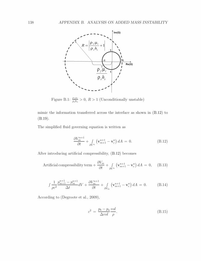
138 APPENDIX B. ANALYSIS ON ADDED MASS INSTABILITY
1+=
ss
if
hR
ρ
µρ
ss
if
hρ
µρ
Im(G)
Re(G)
1
1-1
1
Figure B.1:ρfµi
ρshs> 0, R > 1 (Unconditionally unstable)
mimic the information transferred across the interface as shown in (B.12) to
(B.19).
The simplified fluid governing equation is written as
∂V n+1m
∂t+ ∫
∂V n
(vn+1m+1 − vn
c
)dA = 0. (B.12)
After introducing artificial compressibility, (B.12) becomes
Artificial compressibility term +∂Vm
∂t+ ∫
∂V n
(vn+1m+1 − vn
c
)dA = 0, (B.13)
∫ 1
ρc2pn+1m+1 − pn+1
m
∆tdV +
∂V n+1m
∂t+ ∫
∂Vm
(vn+1m+1 − vn
c
)dA = 0. (B.14)
According to (Degroote et al., 2009),
c2 =pb − pa∆vol
vol
ρ. (B.15)
B.1. ANALYSIS 139
By substituting (B.15) in (B.14), we get
∆vol
pb − pa
pn+1m+1 − pn+1
m
∆t+
∂V n+1m
∂t+ ∫
∂Vm
(vn+1m+1 − vn
c
)dA = 0. (B.16)
To simplify,
∆vol
pb − pa
pn+1m+1 − pn+1
m
∆t≈ ∆vol
∆t≈ V n+1
m+1 − V n+1m
∆t. (B.17)
∂Vm
∂t=
V n+1m − V n
∆t. (B.18)
For validation of (B.16), we refer to (Degroote et al., 2009).
Substituting (B.17) and (B.18) in (B.16), we get
∂V n+1m+1
∂t+ ∫
∂V n
(vn+1 − vn
c
)dA = 0. (B.19)
Therefore, It might be reason able to use dn+1,fm+1 = 1
∆t2(dn+1
m+1,i−2dn+1m,i +dn+1
m−1,i)
instead of dn+1,fm+1 = 1
∆t2(dn+1
m,i − 2dn+1m−1,i + dn+1
m−2,i).
By conducting a similar Von Neumann stability analysis that we have done
for Leap-frog and Euler scheme, but this time with artificial compressibility,
we obtain
ρshs
4t2(dn+1
i − 2dni + dn−1i ) +
ρfµi
4t2(dn+1
i − 2dni + dn−1i ) + a0d
ni = P n
ext,i (B.20)
dn+1i − 2dni + dn−1
i =4t2
(P next,i − a0d
ni
)
ρshs + ρfµi
(B.21)
dn+1i − 2dni + dn−1
i = 0 ∵ 4t2 → 0. (B.22)
140 APPENDIX B. ANALYSIS ON ADDED MASS INSTABILITY
It can be further reduced to
dn+1i = 2dni − dn−1
i . (B.23)
By recalling (B.9),
dn−1i = eia(t+4t)eikx and dni = eia(t+24t)eikx.
Substituting into (B.23), we get
dn+1i =
(2eia24t − eia4t=
)eiateikx, (B.24)
and
|G| =∣∣2eia2∆t − eia∆t
∣∣ . (B.25)
The growth factor in (B.25) is equivalent to a unit circle with origin at (0,0) in a
complex plane. Therefore, it is determined that the solution is unconditionally
stable when applying artificial compressibility.
B.2 Conclusion
In conclusion, explicit calculation of fluid-structure interaction leads to un-
conditional instability. On the contrary, previous studies have demonstrated
that calculation in the implicit way can result in conditional stability. Our
derivation also shows that properties of the problem such as density ratio and
the flexibility of the solid structure can influence the stability significantly.
Moreover, it is demonstrated that stability of the coupling can be maintained
by applying “Artificial compressibility” technique. This numerical manipu-
lation allows the solution to be done explicitly, which therefore reduces the
computational time required to solve FSI problems.
References
Abdelaziz, O. S., Ogilvy, C. S. and Lev, M. (1999). Is there a potential role
for hyoid bone compression in pathogenesis of carotid artery stenosis?,
Surgical Neurology 51(6): 650 – 653.
Alonso, J. J. and Jameson, A. (1994). Fully-implicit time-marching aeroelastic
solutions, AIAA Paper 91-0939 .
ANSYS Inc. 2009. ANSYS CFX-Solver Theory Guide (n.d.).
Badia, S., Quaini, A. and Quarteroni, A. (2008). Modular vs. non-modular
preconditioners for fluid-structure systems with large added-mass ef-
fect, Computer Methods in Applied Mechanics and Engineering 197(49-
50): 4216 – 4232.
Bai, Y., Sun, D. and Lin, J. (2010). Three dimensional numerical simulations of
long-span bridge aerodynamics, using block-iterative coupling and DES,
Computers & Fluids 39(9): 1549 – 1561.
Bathe, K. (1996). Finite element procedures, Prentice-Hall.
Batina, J. T. (1989). Unsteady Euler algorithm with unstructured dynamic
mesh for complex-aircraft aeroelastic analysis, AIAA 89: 1189.
Bendiksen, O. O. (1991). A new approach to computational aeroelasticity,
AIAA Paper 91-0939 .
Bletzinger, K. U., Gallinger, T., Kupzok, A. and Wuchner, R. (2006). Parti-
tioned strategies for optimization in FSI, European Conference on Com-
putational Fluid Dynamics .
141
142 REFERENCES
Blom, F. J. (1998). A monolithical fluid-structure interaction algorithm ap-
plied to the piston problem, Computer Methods in Applied Mechanics and
Engineering 167(3-4): 369 – 391.
Boffi, D. and Gastaldi, L. (2004). Stability and geometric conservation laws
for ALE formulations, Computer Methods in Applied Mechanics and En-
gineering 193(42-44): 4717 – 4739.
Borazjani, I., Ge, L. and Sotiropoulos, F. (2008). Curvilinear immersed bound-
ary method for simulating fluid structure interaction with complex 3D
rigid bodies, Journal of Computational Physics 227(16): 7587 – 7620.
Braun, A. L. and Awruch, A. M. (2009). Aerodynamic and aeroelastic analyses
on the CAARC standard tall building model using numerical simulation,
Computers & Structures 87(9-10): 564 – 581.
Brezzi, F., Lions, J. L. and Pironneau, O. (2001). Analysis of a chimera
method, Comptes Rendus de IAcademie des Sciences. Serie I. Mathema-
tique 332: 655–660.
C. Farhat, P. H. G. and Grandmont, C. (2001). The discrete geometric con-
servation law and the nonlinear stability of ALE schemes for the solu-
tion of flow problems on moving grids, Journal of Computational Physics
174(2): 669–694.
Callaghan, F. M., Soellinger, M., Baumgartner, R. W., Boesiger, D. P. P. and
Kurtcuoglu, V. (2009). The role of the carotid sinus in the reduction of
arterial wall stresses due to head movements–potential implications for
cervical artery dissection, Journal of Biomechanics 42(6): 755–761.
Carlton, A. (2004). A summary study on arbitrary Lagrangian-Eulerian:
methodology, implementation, and application, Technical report, Oregon
State University.
Caro, C. G., Fitz-Gerald, J. M. and Schroter, R. C. (1971). Atheroma and
arterial wall shear observation, correlation and proposal of a shear de-
pendent mass transfer mechanism for atherogenesis., Proceedings of The
Royal Society of London. 177: 109–159.
REFERENCES 143
Carter, F. D. and Baker, A. (1991). Accuracy and stability of a finite element
pseudo compressibility CFD algorithm for incompressible thermal flows,
Numerical Heat Transfer 20: 1–23.
Causin, P., Gerbeau, J. F. and Nobile, F. (2005). Added-mass effect in the
design of partitioned algorithms for fluid-structure problems, Computer
Methods in Applied Mechanics and Engineering 194(42-44): 4506 – 4527.
Cho, J. R., Lee, H. W., Sohn, J. S., Kim, G. J. and Woo, J. S. (2006). Nu-
merical investigation of hydroplaning characteristics of three-dimensional
patterned tire, The European Journal of Mechanics A/Solids 25(6): 914
– 926.
Chorin, A. J. (1967). A numerical method for solving incompressible viscous
flow problems, Journal of Computational Physics 2: 12–26.
Chorin, A. J. (1968). Numerical solution of the Navier-Stokes equations, Math-
ematics of Computation 22: 745–762.
Chung, J. and Hulbert, G. M. (1993). A time integration algorithm for struc-
tural dynamics with improved numerical dissipation: The generalized-α
method., Journal of Applied Mechanics 60(2): 371–375.
Daneshmand, F., Saketi, P. and Khajepour, A. (2005). 3D finite element
analysis of a hydraulic engine mount including fluid-structure interac-
tion, in Chakrabarti, SK and Hernandez, S and Brebbia, CA (ed.),
Fluid structure Interaction and Moving Boundary Problems, Vol. 84 of
WIT TRANSACTIONS ON THE BUILT ENVIRONMENT, Wessex Inst
Technol; Univ La Coruna; WIT Transact Built Environm, WIT PRESS,
ASHURST LODGE, SOUTHAMPTON SO40 7AA, ASHURST, ENG-
LAND, pp. 165–174. 3rd International Conference on Fluid Structure In-
teraction/8th International Conference on Computational Modelling and
Experimental Measurements of Free and Moving Boundary Problems,
Coruna, SPAIN, SEP 19-21, 2005.
144 REFERENCES
Dang, H., Yang, Z. and Li, Y. (2010). Accelerated loosely-coupled CFD/CSD
method for nonlinear static aeroelasticity analysis, Aerospace Science and
Technology 14(4): 250 – 258.
Degroote, J., Bathe, K. J. and Vierendeels, J. (2009). Simulation of fluid-
structure interaction with the interface artificial compressibility method,
International Journal for Numerical Methods in Biomedical Engineering
26: 276–289.
Degroote, J., Bruggeman, P., Haelterman, R. and Vierendeels, J. (2008). Sta-
bility of a coupling technique for partitioned solvers in fsi applications,
Computers & Structures 86(23-24): 2224 – 2234.
Degroote, J., Haelterman, R., Annerel, S., Bruggeman, P. and Vierendeels, J.
(2010). Performance of partitioned procedures in fluid-structure interac-
tion, Computers & Structures 88(7-8): 446 – 457.
Delfino, A., Stergiopulos, N., Moore, J. E. and Meister, J. J. (1997). Residual
strain effects on the stress field in a thick wall finite element model of the
human carotid bifurcation, Journal of Biomechanics 30(8): 777–786.
Ding, Z., Wang, K., Li, J. and Cong, X. (2001). Flow field and oscillatory
shear stress in a tuning-fork-shaped model of the average human carotid
bifurcation, Journal of Biomechanics 34(12): 1555–1562.
Donea, J., Huerta, A., Ponthot, J. P. and Rodriguez-Ferran, A. (2004). Arbi-
trary Lagrangian-Eulerian methods In encyclopedia of computational me-
chanics Vol. 1: Fundamentals, John Wiley & Sons.
Dowell, E. H. and Hall, K. C. (2001). Modelling of fluid-structure interaction,
Ann Rev Fluid Mech 33: 445–490.
Eloy, C., Souilliez, C. and Schouveiler, L. (2007). Flutter of a rectangular
plate, Journal of Fluids and Structures 23(6): 904 – 919.
Eriksson, L. E. (1982). Generation of boundary-conformation grids around
wing-body configurations using transfinite interpolation, AIAA 20: 1313–
1320.
REFERENCES 145
Falk, E. (1991). Coronary thrombosis: pathogenesis and clinical manifesta-
tions., American Journal of Cardiology 68(7): 28–35.
Falk, E. (1992). Why do plaques rupture ?, Monograph - American Heart
Association 86: III.30–III.42.
Farhat, C. and Lesoinne, M. (2000). Two efficient staggered algorithms for
the serial and parallel solution of three-dimensional nonlinear transient
aeroelastic problems, Computer Methods in Applied Mechanics and En-
gineering 182(3-4): 499 – 515.
Farhat, C., Lesoinne, M. and LeTallec, P. (1998). Load and motion transfer al-
gorithms for fluid/structure interaction problems with non-matching dis-
crete interfaces: Momentum and energy conservation, optimal discretiza-
tion and application to aeroelasticity, Computer Methods in Applied Me-
chanics and Engineering 157: 95–114.
Felippa, C. A. and Park, K. C. (1980). Staggered transient analysis proce-
dures for coupled mechanical systems: Formulation, Computer Methods
in Applied Mechanics and Engineering 24(1): 61 – 111.
Felippa, C. A., Park, K. C. and Farhat, C. (2001). Partitioned analysis of
coupled mechanical systems, Computer Methods in Applied Mechanics
and Engineering 190(24-25): 3247 – 3270.
Formaggia, L., Gerbeau, J. F., Nobile, F. and Quarteroni, A. (2001). Nu-
merical treatment of defective boundary conditions for the navier-stokes
equation, INRIA Research Report No. 4093 .
Forster, C., Wall, W. A. and Ramm, E. (2007). Artificial added mass in-
stabilities in sequential staggered coupling of nonlinear structures and
incompressible viscous flows, Computer Methods in Applied Mechanics
and Engineering 196(7): 1278 – 1293.
Friedman, M. H., Deters, O. J., Bargeron, C. B. and Mark, G. M. H.
F. F. (1986). Shear-dependent thickening of the human arterial intima,
Atherosclerosis 60: 161–171.
146 REFERENCES
Friedman, M. H., Deters, O. J., Bargeron, C. B. and Mark, G. M. H. F. F.
(1989). A biologically plausible model of thickening of arterial intima
undershear, Arteriosclerosis 9: 511–522.
Gerstenberger, A. and Wall, W. A. (2008). Enhancement of fixed-grid methods
towards complex fluid-structure interaction applications, International
Journal for Numerical Methods in Fluids 57: 1227–1248.
Giannoglou, G. D., Chatzizisis, Y. S., Zamboulis, C., Parcharidis, G. E.,
Mikhailidis, D. P. and Louridas, G. E. (2008). Elevated heart rate and
atherosclerosis: An overview of the pathogenetic mechanisms, Interna-
tional Journal of Cardiology 126: 302 – 312.
Giddens, D. P., Zarin, C. K. and Glagov, S. (1993). The role of fluid me-
chanics in the localization and detection ofatherosclerosis., Journal of
Biomechanical Engineering 115(4B): 588–94.
Glagov, S., Zarins, C. K., Giddens, D. P. and Ku, D. N. (1989). Mechanical
factors in thepathogenesis, localization and evolution of atherosclerotic
plaques, Springer-Verlag, N.Y.
Glowinski, R., He, J. W., Lozinski, A., Rappaz, J. and Wagner, J. (2005). Fi-
nite element approximation of multi-scale elliptic problems using patches
of elements, Numerical Mathematics .
Grant, E. G., Benson, C. B., Moneta, G. L., Alexandrov, A. V., Baker, J. D.,
Bluth, E. I., Carroll, B. A., Eliasziw, M., Gocke, J., Hertzberg, B. S.,
Katanick, S., Needleman, L., Pellerito, J., Polak, J. F., Rholl, K. S.,
Wooster, D. L. and Zierler, R. E. (2003). Carotid artery stenosis: Gray-
scale and doppler US diagnosis - society of radiologists in ultrasound
consensus conference 1, Radiology 229(2): 340–346.
Gregory, A. F. and Michael, C. F. (2008). Arteriosclerosis: Rethinking the
current classification, Archives of Pathology and Laboratory Medicine
133(8): 1309–1316.
REFERENCES 147
Grohmann, B. A., Dornberger, R. and Dinkler, D. (1997). Time-discontinuous
stabilized space-time finite elements for aeroelasticity, Fluid-Structure In-
teraction, Flow-Induced Vibrations and Noise 3: AD53–3.
Guidoboni, G., Glowinski, R., Cavallini, N. and Canic, S. (2009). Stable
loosely-coupled-type algorithm for fluid-structure interaction in blood
flow, Journal of Computational Physics 228(18): 6916 – 6937.
Guillard, H. and Farhat, C. (2000). On the significance of the geometric con-
servation law for flow computations on moving meshes, Comput. Methods
Appl. Mech.Eng. 190(11-12): 1467–1482.
Hall, K. C., Thomas, J. P. and Dowell, E. H. (2000). Proper orthogonal
decomposition technique for transonic unsteady aerodynamic flows, AIAA
38(10): 1853–1862.
Hariton, I., deBotton, G., Gasser, T. C. and Holzapfel, G. A. (2007). Stress-
modulated collagen fiber remodeling in a human carotid bifurcation, Jour-
nal of Theoretical Biology 248(3): 460–470.
Hart, J. D., Baaijens, F. P. T., Peters, G. W. M. and Schreurs, P. J. G.
(2003). A computational fluid-structure interaction analysis of a fiber-
reinforced stentless aortic valve, Journal of Biomechanics 36(5): 699 –
712. Cardiovascular Biomechanics.
Hartwich, P. M. and Agrawal, S. (1997). Method for perturbing multi-block
patched grids in aeroelastic and design optimization applications, AIAA
97: 2038.
Hatamura, Y. (1996). Zoku-Zoku Jissai-no Sekkei (Practical Design III), Tech-
nical report, The Nikkan Kogyo Shimbun, LTD.
Hieber, S. E. and Koumoutsakos, P. (2008). An immersed boundary method
for smooth particle hydrodynamics of self-propelled swimmers, Journal
of Computational Physics 227: 8636–8654.
148 REFERENCES
Hirt, C. W., Cook, J. L. and Butler, T. D. (1970). A Lagrangian method
for calculating the dynamics of an incompressible fluid with free surface,
Journal of Computational Physics 5: 103–124.
Hron, J. and Turek, S. (2006). A monolithic FEM/multigrid solver for ALE
formulation of fluid structure interaction with application in biomechan-
ics, Fluid-Structure Interaction: Modelling, Simulation, Optimisation
53: 146–170.
Hubner, B., Walhorn, E. and Dinkler, D. (2004). A monolithic approach
to fluid-structure interaction using space-time finite elements, Computer
Methods in Applied Mechanics and Engineering 193(23-26): 2087 – 2104.
Irons, B. and Tuck, R. C. (1969). A version of the aitken accelerator for
computer implementation, International Journal for Numerical Methods
in Engineering 1: 275–277.
Jacobson, M. (1999). Fundamentals of atmospheric modeling, Cambridge Uni-
versity Press.
Jaiman, R. J. (2007). Accuracy and stability of transient multiphysics simula-
tions, PhD thesis, University of Illinois.
Jarvinen, E., Lyly, M., Ruokolainen, J. and Raback, P. (2001). Three dimen-
sional fluid-structure interaction modeling of blood flow in elastic arteries,
Eccomas Computational Fluid Dynamics Conference .
Joshi, A. K., Leask, R. L., Myers, J. G., Ojha, M. and Ethier, J. B. C. R.
(2004). Intimal thickness is not associated with wall shear stress patterns
in the human right coronary artery, Arteriosclerosis, Thrombosis, and
Vascular Biology 24(12): 2408–2413.
Kalro, V. and Tezduyar, T. E. (2000). A parallel 3D computational method
for fluid-structure interactions in parachute systems, Computer Methods
in Applied Mechanics and Engineering 190(3-4): 321 – 332.
Kamakoti, R. and Shyy, W. (2004). Fluid-structure interaction for aeroelastic
applications, Progress in Aerospace Sciences 40(1): 535–558.
REFERENCES 149
Kaunas, R. and Hsu, H. J. (2009). A kinematic model of stretch-induced
stress fiber turnover and reorientation, Journal of Theoretical Biology
257(2): 320–330.
Kaunas, R., Usami, S. and Chien, S. (2006). Regulation of stretch-
induced JNK activation by stress fiber orientation, Cellular Signalling
18(11): 1924–1931.
Kawahara, M. and Ohmiya, K. (1985). Finite element analysis of density flow
using velocity correction method, International Journal for Numerical
Methods in Fluids 5: 981–993.
Kleinstreuer, C., Hyun, S., Buchanan, J. R., Longest, P. W., Archie, J. P.
and Truskey, G. A. (2001). Hemodynamic parameters and early intimal
thickening in branching blood vessels., Critical Reviews in Biomedical
Engineering 29(1): 1–64.
Knight, J. J., Lucey, A. D. and Shaw, C. T. (2010). Fluid-structure interaction
of a two-dimensional membrane in a flow with a pressure gradient with
application to convertible car roofs, Journal of Wind Engineering and
Industrial Aerodynamics 98(2): 65 – 72.
Koobus, B. and Farhat, C. (1999). Second-order accurate and geometrically
conservative implicit schemes for flow computations on unstructured dy-
namic meshes, Computer Methods in Applied Mechanics and Engineering
170(1-2): 103–129.
Korteweg, D. J. (1878). Uber die Fortpflanzungsgeschwindigkeit des Schalles
in elastischen Rohren, Annals of Physics 5: 525.
Ku, D. N. and Giddens, D. P. (1983). Pulsatile flow in a model carotid bifur-
cation, Arteriosclerosis, Thrombosis, and Vascular Biology 3(1): 31–39.
Ku, D. N., Giddens, D. P., Zarins, C. K. and Glagov, S. (1985). Pulsatile flow
and atherosclerosis in the human carotid bifurcation.positive correlation
between plaque location and low oscillatingshear stress, Arteriosclerosis,
Thrombosis, and Vascular Biology 5(3): 293–302.
150 REFERENCES
Kuttler, U. and Wall, W. (2008). Fixed-point fluid-structure interaction solvers
with dynamic relaxation, Computational Mechanics 43(1): 61–72.
l Farhat, C., van der Zee, K. G. and Geuzaine, P. (2006). Provably second-order
time-accurate loosely-coupled solution algorithms for transient nonlinear
computational aeroelasticity, Computer Methods in Applied Mechanics
and Engineering 195(17-18): 1973 – 2001. Fluid-Structure Interaction.
Lau, K. D., Diaz, V., Scambler, P. and Burriesci, G. (2010). Mitral valve
dynamics in structural and fluid-structure interaction models, Medical
Engineering & Physics In Press, Corrected Proof: –.
Lee, D. and Chiu, J. J. (1996). Intimal thickening under shear in a carotid
bifurcation-a numerical study, Journal of Biomechanics 29(1): 1–11.
Lee, K. W. and Xu, X. Y. (2002). Modelling of flow and wall behaviour in a
mildly stenosed tube, Medical Engineering & Physics 24(9): 575–586.
Lesoinne, M. and Farhat, C. (1996). Geometric conservation laws for flow
problems with moving boundaries and deformation meshes, and their
impact on aeroelastic computations, Arteriosclerosis, Thrombosis, and
Vascular Biology 134(1-2): 71–90.
Masud, A. and Hughes, T. J. R. (1997). A space-time Galerkin/least-squares fi-
nite element formulation of the navier-stokes equations for moving domain
problems, Arteriosclerosis, Thrombosis, and Vascular Biology 146(1-
2): 91 – 126.
Matthies, H. G., Niekamp, R. and Steindorf, J. (2006). Algorithms for strong
coupling procedures, Computer Methods in Applied Mechanics and Engi-
neering 195(17-18): 2028 – 2049. Fluid-Structure Interaction.
Merkle, C. and Athavale, M. (1987). Time-accurate unsteady incompressible
flow algorithm based on artificial compressibility, AIAA 87: 397–407.
Michler, C. (2005). Efficient numerical methods for fluid-structure interaction,
PhD thesis, Delft University.
REFERENCES 151
Michler, C., Hulshoff, S. J., van Brummelen, E. H. and de Borst, R. (2004). A
monolithic approach to fluid-structure interaction, Computers and Fluids
33: 839–848.
Mizukami, A. and Tsuchiya, M. (1984). A finite element method for the three
dimensional non-steady Navier-Stokes equations, International Journal
for Numerical Methods in Fluids 4: 349–357.
Moens, A. (1878). Die Pulskurve, Brill, Leiden.
Nerem, R. M. (1992). Vascular fluid mechanics, the arterial wall, and
atherosclerosis, Journal of Biomechanical Engineering 114(3): 274–282.
Nobili, M., Morbiducci, U., Ponzini, R., Gaudio, C. D., Balducci, A., Grigioni,
M., Montevecchi, F. M. and Redaelli, A. (2008). Numerical simulation of
the dynamics of a bileaflet prosthetic heart valve using a fluid-structure
interaction approach, Journal of Biomechanics 41(11): 2539 – 2550.
Palatini, P. (1999). Heart rate as a risk factor for atherosclerosis and cardiovas-
cular mortality: the effect of antihypertensive drugs, Drugs 57: 713–724.
Patankar, S. V. (1980). Numerical heat transfer and fluid flow, Hemisphere.
Perktold, K., Peter, R. O., Resch, M. and Langs, G. (1991). Pulsatile non-
newtonian blood flow in three-dimensional carotid bifurcationmodels: a
numerical study of flow phenomena under different bifurcationangles,
Journal of Biomedical Engineering 13(6): 507–515.
Peskin, C. S. (2002). The immersed boundary method, Acta Numerica
11: 479–517.
Peterson, N. (1999). An algorithm for assembling overlapping grid systems,
SIAM Journal on Scientific Computing 20: 1995–2022.
Peyret, R. (1976). Unsteady evolution of a horizontal jet in a stratified fluid,
Journal of Fluid Mechanics 78(1): 49–63.
152 REFERENCES
Piperno, S. (1997). Explicit/implicit fluid/structure staggered procedures
with a structural predictor and fluid subcycling for 2D inviscid aeroelas-
tic simulations, International Journal for Numerical Methods in Fluids
25: 12071226.
Piperno, S. (2001). Partitioned procedures for the transient solution of cou-
pled aeroelastic problems - part II: Energy transfer analysis and three-
dimensional applications, Computer Methods in Applied Mechanics and
Engineering 190: 31473170.
Piperno, S., Farhat, C. and Larrouturou, B. (1995). Partitioned procedures
for the transient solution of coupled aeroelastic problems - part I: Model
problem, theory and two-dimensional applications, Computer Methods in
Applied Mechanics and Engineering 124: 79112.
Price, J. F. (2006). Lagrangian and Eulerian representations of fluid flow:
Kinematics and the equations of motion, Technical report, Woods Hole
Oceanopraphic Institution, Woods Hole, MA.
Quan, L., Xu, X., Ben, A., Simon, A. and D. H. Alun, D. H. V. H. A. (2000).
Reconstruction of blood flow patterns in a human carotid bifurcation: A
combined CFD and MRI study, Journal of Magnetic Resonance Imaging
11(3): 299–311.
Raback, P., Ruokolainen, J., Lyly, M. and Jarvinen, E. (2001). Fluid-structure
interaction boundary conditions by artificial compressibility, European
Conference on Computational Fluid Dynamics ECCOMAS .
Ramaswamy, B., Kawahara, M. and Nakayama, T. (1986). Lagrangian finite
element method for the analysis of two-dimensional sloshing problems,
International Journal for Nmerical Methods in Fluids 6: 659–670.
Ramnarine, K., Hartshorne, T., Sensier, Y., Naylor, M., J.Walker, Naylor,
A., Panerai, R. and Evans, D. (2003). Tissue doppler imaging of carotid
plaque wall motion: a pilot study, Cardiovascular Ultrasound 1(1): 17.
REFERENCES 153
Richter, T. and Wick, T. (2010). Finite elements for fluid-structure interaction
in ALE and fully Eulerian coordinates, Computer Methods in Applied
Mechanics and Engineering 199(41-44): 2633 – 2642.
Rifai, S. M., Johan, Z., Wang, W.-P., Grisval, J.-P., Hughes, T. J. and Fer-
encz, R. M. (1999). Multiphysics simulation of flow-induced vibrations
and aeroelasticity on parallel computing platforms, Computer Methods in
Applied Mechanics and Engineering 174(3-4): 393 – 417.
Robinson, B. A., Batina, J. T. and Yang, H. T. Y. (1991). Aeroelastic analysis
of wings using the euler equations with a deforming mesh, Journal of
Aircraft 32: 416–422.
Rogers, S. E., Kwak, D. and Kaul, U. (1987). On the accuracy of the pseudo-
compressiblility method in solving the incompressible navier-stokes equa-
tions, Applied Mathematical Modelling 11: 35–44.
Sagatun, S. I., Herfjord, K. and Holmas, T. (2002). Dynamic simulation of
marine risers moving relative to each other due to vortex and wake effects,
Journal of Fluids and Structures 16(3): 375 – 390.
Salzar, R. S., Thubrikar, M. J., Eppink, R. T. and Richard, T. (1995).
Pressure-induced mechanical stress in the carotid artery bifurca-
tion:a possible correlation to atherosclerosis, Journal of Biomechanics
28(11): 1333–1340.
Samuel, A., Jens, V., Nikolaj, E., andK. Anette, F. E.-T., William, P., Er-
ling, F. and Kim, W. (2008). Mechanical stresses in carotid plaques us-
ing mri-based fluid-structure interaction models, Journal of Biomechanics
41(8): 1651–1658.
Samuel, A. K., Jens, V. N., Anders, K. N., Anette, K., P.William, P., Erling,
F. and Kim, W. Y. (2007). Stresses in carotid plaques using MRI-based
fluid structure interaction models, Proceedings of the COMSOL Users
Conference 2007 .
154 REFERENCES
Schneider, G. E., Raithby, G. D. and Yavanovich, M. M. (1978). Finite element
solution procedure for solving the incompressible Navier-Stokes equations
using order interpolation, Numerical Heat Transfer 1: 435–451.
Schuster, D. M., Vadyak, J. and Atta, E. (1990). Static aeroelastic analy-
sis of fighter aircraft using a three-dimensional Navier-Stokes algorithm,
Journal of Aircraft 27: 820–825.
Senes, S. (2006). How we manage stroke in Australia?, Technical report, Aus-
tralian Institute of Health and Welfare, Canberra.
Shabana, A. (2008). Computational continuum mechanics, Cambridge Uni-
versity Press, New York, USA.
Shangguan, W. B. and Lu, Z. H. (2004). Modelling of a hydraulic engine
mount with fluid-structure interaction finite element analysis, Journal of
sound and vibration 275(1-2): 193–221.
Silva, W. and Bartels, R. (2004). Development of reduced-order models for
aeroelastic analysis and flutter prediction using the CFL3Dv6.0 code,
Journal of Fluids and Structures 19(6): 729 – 745.
Sinz, W. and Hermann, S. (2008). The development of a 3D-Navier-Stokes code
for the simulation of an airbag inflation, Simulation Modelling Practice
and Theory 16(8): 885 – 899. EUROSIM 2007.
Solving FSI Applications using Workbench, ANSYS Mechanical and CFX
(n.d.).
Souli, M., Ouahsine, A. and Lewin, L. (2000). ALE formulation for fluid-
structure interaction problems, Computer Methods in Applied Mechanics
and Engineering 190(5-7): 659 – 675.
Steger, J., Dougherty, F. and Benek, J. (1983). A Chimera grid scheme, in
K. N. Ghia and U. Ghia (eds), ASME FED, Vol. 5 of Advances in Grid
Generation.
Storti, M. A., Nigro, N. M., Paz, R. R. and Dalcin, L. D. (2009). Strong
coupling strategy for fluid-structure interaction problems in supersonic
REFERENCES 155
regime via fixed point iteration, Journal of Sound and Vibration 320(4-
5): 859 – 877.
Strang, G. (2007). Computational science and engineering, Wellesley.
Sun, D., Owen, J. S., Wright, N. G. and Liaw, K. F. (2008). Fluid-structure
interaction of prismatic line-like structures, using LES and block-iterative
coupling, Journal of Wind Engineering and Industrial Aerodynamics
96(6-7): 840 – 858. 5th International Colloquium on Bluff Body Aerody-
namics and Applications.
Tada, T. and Tarbell, M. (2005). A computational study of flow in a compli-
ant carotid bifurcation - stress phase angle correlation with shear stress,
Annals of Biomedical Engineering 33(9): 1202–1212.
Takashi, N. (1994). ALE finite element computations of fluid-structure interac-
tion problems, Computer Methods in Applied Mechanics and Engineering
112(1-4): 291 – 308.
Tallec, P. L. and Mouro, J. (2001). Fluid structure interaction with large
structural displacements, Computer Methods in Applied Mechanics and
Engineering 190: 30393068.
Tang, D. (2004). 3D MRI-based multicomponent FSI models for atheroscle-
rotic plaques, Annals of Biomedical Engineering 32(7): 947–960.
Tang, D., Yang, C., Mondal, S., Liu, F., Canton, G., T.S.Hatsukami and Yuan,
C. (2008). A negative correlation between human carotid atherosclerotic
plaque progression and plaque wall stress: In vivo MRI-based 2D/3D FSI
models, Journal of Biomechanics 41(4): 727–736.
Tardif, J. (2009). Heart rate and atherosclerosis, European Heart Journal
Supplements 11: D8–D12.
Tezduyar, T., Sathe, S., Keedy, R. and Stein, K. (2006). Space-time finite
element techniques for computation of fluid-structure interactions, Com-
puter Methods in Applied Mechanics and Engineering 195: 2002–2007.
156 REFERENCES
Thubrikar, M. and Robicsek, F. (1995). Pressure-induced arterial wall stress
and atherosclerosis, Annals of Thoracic Surgery 59(6): 1594–1603.
Torii, R., Wood, N. B., Hadjiloizou, N., Dowsey, A. W., Wright, A. R., Hughes,
A. D., Davies, J., Francis, D. P., Mayet, J., Yang, G.-Z., Thom, S.
A. M. and Xu, X. Y. (2009). Fluid-structure interaction analysis of a
patient-specific right coronary artery with physiological velocity and pres-
sure waveforms, Communications in Numerical Methods in Engineering
25: 565–580.
Valencia, A. (2006). Unsteady flow and mass transfer in models of stenotic ar-
teries, International Communications in Heat and Mass Transfer 33: 966–
975.
van Brummelen, E. H. and de Borst, R. (2005). On the nonnormality of
subiteration for a fluid-structure-interaction problem, SIAM Journal on
Scientific Computing 27: 599–621.
van Brummelen, E. H., Michler, C. and de Borst, R. (2003). Energy con-
servation under incompatibility for fluid-structure interaction problems,
Computer Methods in Applied Mechanics and Engineering 192: 2727–
2748.
Vierendeels, J., Lanoye, L., Degroote, J. and Verdonck, P. (2007). Implicit
coupling of partitioned fluid-structure interaction problems with reduced
order models, Computers & Structures 85(11-14): 970 – 976. Fourth MIT
Conference on Computational Fluid and Solid Mechanics.
Wall, W. A., Forster, C., Neumann, M. and Ramm, E. (2006). Advances in
fluid-structure interaction, 17th International Conference on the Appli-
cation of Computer Science and Mathematics in Architecture and Civial
Engineering .
Wall, W. A., Gerstenberger, A., Gamnitzer, P., Forster, C. and Ramm, E.
(2006). Large deformation fluid-structure interaction: Advances in ALE
methods and new fixed grid approaches in fluid-structure interaction:
Modelling, simulation, optimization, Springer: Berlin.
REFERENCES 157
Wang, W. Q. and Yan, Y. (2010). Strongly coupling of partitioned fluid-
solid interaction solvers using reduced-order models, Applied Mathemati-
cal Modelling 34(12): 3817 – 3830.
Wentzel, J. J., Janssen, E., Vos, J., Schuurbiers, J. C. H., Krams, R., Serruys,
P. W., de Feyter, P. J. and Slager, C. J. (2003). Extension of increased
atherosclerotic wall thickness into high shear: stress regions is associated
with loss of compensatory remodeling, Circulation 108(1): 17–23.
Willcox, K. and Peraire, J. (2002). Balanced model reduction via the proper
orthogonal decomposition, AIAA 40(11): 2323–2330.
Wong, K. K. L., Mazumdar, J., Pincombe, B., Sanders, S. G. W. P. and
Abbott, D. (2006). Theoretical modeling of micro-scale biological phe-
nomena in humancoronary arteries, Medical & Biological Engineering &
Computing 44(11): 971–982.
Wong, K. K. L., Tu, J. Y., Mazumdar, J. and Abbott, D. (2010). Modelling of
blood flow resistance for an atherosclerotic arterywith multiple stenoses
and poststenotic dilatations, ANZIAM Journal E 51: C66–C82.
Wood, C., Gil, A. J., Hassan, O. and Bonet, J. (2008). Partitioned block-
gauss-seidel coupling for dynamic fluid-structure interaction, Computers
& Structures In Press, Corrected Proof: –.
Wood, W. L., Bossak, M. and Zienkiewicz, O. C. (1981). An alpha modifica-
tion of newmark method, International Journal of Numerical Method in
Engineering 15: 1562.
Wuchner, R., Kupzok, A. and Bletzinger, K. U. (2007). A framwork for sta-
bilized partitioned analysis of thin membrane-wind interaction, Interna-
tional Journal of Numerical Methods in Fluids 54: 945–963.
Wylie, E. B. and Streeter, V. L. (1983). Fluid transients, FEB Press, Michigan.
Xia, G. H., Zhao, Y. and Yeo, J. H. (2009). Parallel unstructured multigrid
simulation of 3D unsteady flows and fluid-structure interaction in me-
chanical heart valve using immersed membrane method, Computers &
158 REFERENCES
Fluids 38(1): 71 – 79.
Xue, Y. J., Gao, P. Y., Duan, Q., Lin, Y. and Dai, C. B. (2008). Preliminary
study of hemodynamic distribution in patient-specific stenotic carotid bi-
furcation by image-based computational fluid dynamics, Acta Radiologica
49(5): 558–565.
Yamamoto, C. T., Meneghini, J. R., Saltara, F., Fregonesi, R. A. and Ferrari,
J. A. (2004). Numerical simulations of vortex-induced vibration on flexible
cylinders, Journal of Fluids and Structures 19(4): 467 – 489.
Zarins, C. K., Giddens, D. P., Bharadvaj, B. K., Mabon, V. S. S. R. F. and
Glagov, S. (1983). Carotid bifurcation atherosclerosis. quantitative cor-
relation ofplaque localization with flow velocity profiles and wall shear
stress., Circulation Research 53(4): 502–14.
Zhang, L., Gerstenberger, A., Wang, X. and Liu, W. K. (2004). Immersed
finite element method, Computer Methods in Applied Mechanics and En-
gineering 193: 2051–2067.
Zhang, Q. and Hisada, T. (2001). Analysis of fluid-structure interaction prob-
lems with structural buckling and large domain changes by ALE finite
element method, Computer Methods in Applied Mechanics and Engineer-
ing 190(48): 6341 – 6357.
Zhao, S. Z., Ariff, B., Long, Q., Hughes, A. D., Thom, S. A., Stanton, A. V.
and Xu, X. Y. (2002). Inter-individual variations in wall shear stress and
mechanical stress distributions at the carotid artery bifurcation of healthy
humans, Journal of Biomechanics 35(10): 1367 – 1377.