Report No. FRA/ORD-80/52-1Volume 1

PERFORMANCE OF A LINEAR SYNCHRONOUS MOTOR

WITH LAMINATED TRACK POLES AND WITH VARIOUS MISALIGNMENTS

General Electric Company P.0. Box 43

Schenectady, N.Y. 12305

William R. Mischler Thomas A. Nondahl

SEPTEMBER 1980

Document is available to the public through the National Technical Information Service

Springfield, Virginia 22161

U.S. D E P A R T M E N T OF TRANSPO R T A TI O N FEDERAL RAILROAD ADMINISTRATION

Office of Research and Development Washington, D.C. 20590

Prepared for

GENERAL^ ELECTRIC

NOTICE

This document is disseminated under sponsorship of the Department of Transportation in the interest of infor­mation exchange. The United States Government assumes no liability for its contents or use thereof.

The contents of this report reflect the views of General Electric Corporate Research and Development, which is responsible for the facts and the accuracy of the data presented herein. The contents do not necessarily re­flect the official views or policy of the Department of Transportation. This report does not constitute a stan­dard, specification, or regulation.

The United States Government does not endorse products or manufacturers. Trade or manufacturers' names appear herein solely because they are considered essential to the object of this report.

LIST OF RELATED REPORTS

All experimental and analytical work on linear electric motors, both synchronous and induction, performed by the General Electric Company under contract DOT-FR-64147 is contained in the following four reports:

Report No. FRA/ORD - 80/52W.R. Mischler and T.A, Nondahl, Performance of a Linear Synchronous Motor with Laminated Track Poles and w i t h Various Misalignments, The General Electric Company, Sept.-1980.

Volume 1 - This volume contains a description and summary of the linear ' synchronous motor work.

Volumes 2, 3, 4, 5, 6 - These volumes constitute Appendix I, and containall test data and computer runs on the linear synchronous motor.

Report No. FRA/ORD - 80/53G.B. Kliman, W.R. Mischler, and W.R. Oney, Performance of a Single-Sided Linear Induction Motor with Solid Back Iron and with Various Misalignments, The General Electric Company, Sept. T980.

Volume I - This volume, contains a description and summary of the linear induction motor work.

Volume II, Appendix B - Part 1 - This volume contains the first part of thereduced data on the linear induction motor work.

Volume II, Appendix B - Part 2 - This volume contains the second part ofthe reduced data on the linear induction motor work.

Report Wo, FRA/ORD -80/54T.A. Nondahl and E. Richter, Comparisons Between Designs for Single-Sided Linear Electric Motors: Homopolar Synchronous and Induction, The General Electric Company, Sept.1980. (This report is complete in one volume.)

Report No. FRA/ORD - 80/73G.B. Kliman, D.G. Elliott, V.B. Honsinger, T.A. Lipo, W.R. Mischler, T.A. Nondahl, and W.R. Oney, Performance of a Single-Sided Linear Induction Motor with Solid Back Iron and with Various Rail Configurations/Evaluation of the Claw- • Pole Linear Synchronous Motor and Performance of the Homopolar Linear Synchronous Motor with Solid-Iron Poles, The General Electric Company, Sept. 1980.

Volume 1 - This volume contains various experimental and analytical studies of three types of single-sided linear motors: induction, claw- pole, and homopolar synchronous. ^

Volume 2 - This volume contains all experimental runs connected with thestudies of Volume 1.

T E C H N I C A L REPORT S T A N D A R D TITLE P A G E

I. Report No. .FRA/ORD- 80/52-1 2. Government Accession No. 3. Recipient's Catalog No.

4. Title and SubtitleP e r f o r m a n c e o f a L i n e a r S y n c h r o n o u s M o t o r

w i t h L a m i n a t e d T r a c k P o l e s a n d w i t h V a r i o u s

M i s a l i g n m e n t s

5. Report Date________September 19806. Performing Organization Code

7. Author(s) william R. Mischler and Thomas A. Nondahl 8. Performing Organization Report No,SRD-78-102

9. Performing Organization Name and AddressGeneral Electric Company Corporate Research and Development P.0. Box 43Schenectady, New York 12301

10. Work Unit No.

11. Contract or Grant No.DOT-FR-64147

12. Sponsoring A g e n c y Name a n d AddressU.S. Department'of Transportation Federal Railroad Administration Office of Research and Development Washington, D.C. 20590

13. Type of Report and Period CoveredPhase I - Final Report September 15, 1975 - June 30, 1978

14. Sponsoring Agency Code

15. Supplementary Notes

16. AbstractA test facility was designed and built to measure the performance of a

single-sided high speed homopolar Linear Synchronous Motor with laminated rpole pieces over a wide range of frequency and excitation levels. The facility was instrumented to measure performance at the machine terminals, ■flux density in the air gap and machine, and forces in all six axes. The machine was tested under nominal conditions and with perturbations in five .degrees of freedom: air gap, lateral, pitch, roll, and yaw. Equivalent circuit parameters and flux form coefficients were measured and compared to design values. Poor correlation forced a revision of the design programs. The modeling of the finite interpolar gap and interpolar leakage flux led to good agreement between test and revised design values. The test data show a ?:high power factor, the absence of end effects, and a strong tendency of the machine to remain properly aligned relative to the track, with the exception of a destabilizing pitch torque.

17. "Key Words (Selected by Author(s))Linear synchronous motors Linear electric motors High-speed ground transportation

18. Distribution StatementDocument is available to the public through the National Technical In­formation Service, Springfield, VA 22161-

19. Security Classif. (of this report) 20. Security Classif. (of this page) 21. No. of Pages 22. PriceUNCLASSIFIED UNCLASSIFIED 115

l

GENERAL ELECTRIC

TABLE OF CONTENTS

Section Page1 INTRODUCTION AND MACHINE DESIGN SUMMARY......... . 1-1

Electromagnetic Design . . ......................1-1Stator . ’....................................... 1-4Stator Winding ................................. 1-4Stator Core Construction . . . . . . . . . . . . 1-4DC Field Winding .......... . . . . . . . . . . 1-6

Synchronous Motor Design and Fabrication: Rotor. . 1-8- Factor of Safety . . . . . . . . . . . . . . . . 1-8

Design . .................................... 1-82 OPEN CIRCUIT AND SHORT CIRCUIT TESTS . . ........ . 2-1

Friction and Windage Corrections . . . . . . . . . 2-1Open Circuit Voltage and Losses. ...................2-1Short Circuit Current and Losses ................ 2-6

3 MACHINE PERFORMANCE UNDER LOAD .......................3-1Motoring Performance . . . . . . . . . . . . . . . 3-1Commutation Delay. . . . . . . . . . . . ......... 3-7Generating Tests . . . . . ...................... 3-15

4 G-TABLE TESTS. . . . . . . . . ........ . ........ 4-1Variation of Air Gap ........................ . . 4-2Lateral Offsets....................... 4-7

Yaw Angle Displacements. ................ . 4-10Roll Angle Displacements .......... . . . . . . 4-10Pitch Angle Displacements. ................ .. . 4-10

5 RESISTANCE, REACTANCE, FORCE AND FLUX MEASUREMENTS . 5-1DC Resistance Measurements . . . . . . . . . . . . 5-1Forces with DC Armature Current..................5-1D-Axis and Q-Axis Reactances . . . . . . . . . . . 5-3Commutating Reactance Measurement................5-8Flux Measurement ............................ . . 5-9DC Flux Distribution . . . . . . . . . . . . . . . 5-9Initial Air Gap Flux Tests . .................... 5-12Air Gap Flux at Operating Speeds.............. 5-15Track Pole Flux............................... 5-16

Integrated Track Coil Signals....................5-186 MODIFICATIONS AND CORRECTIONS TO THE HOMOPOLAR

LSM DESIGN PROGRAM............................. .. 6-1Form Factors Km and Ku . . . . .................. 6-1Dependence of Km and Ku on Air Gap Ratio........6-2Interarmature Flux Correction......... 6-5Program Sequence to Correct Km and Ku. . . . . . 6-8Verification of Corrections for 112 kW Test LSM. . 6-9

iii

GENERAL & ELECTRIC

TABLE OF CONTENTS (CONT’D)

Section Page7 EXPERIMENTAL DATA............. 7-1

Data Acquisition ............ ..................Catalog of Test Data...........................7-17-9

8 CONCLUSION . . i .............................................................. 8 - 1

LIST O F I L L U S TRATIONS

Figure -

1 - 1 Connection Diagram and Coil Arrangement. . . . . . . 1-51 - 2 Slot, Tooth and Conductor Layout!for 112 kW

Air-Cooled Homopolar Machine ............. ... . ' . . 1 - 6

1-3 Stator and Support Assembly. . . ........... .1-4 Stator and Support Assembly.................. 1 - 8

1-5 Rotor Design for the Synchronous Motor . * ............... 1-91 - 6 Rotor Design for the Synchronous Motor (Continued) . 1 - 1 0

2 - 1 * - LSM Laminated Track Friction and Windage Torque Vs. Speed Near 240 and 600 rpm Operating Conditions. . . 2 - 2

2 - 2 LSM Laminated Track Friction and Windage Torque Vs. Speed Near 1530 rpm Operating Conditions .................. 2 - 2

2-3 LSM Laminated Track Line-to-Neutral Voltages at 75 Ampere Field - 240 rpm (12.4 mps) 60 Hertz. . . . 2-3

2-4 I.SM Laminated Track Open Circuit Voltage Vs. Field Current and Air Gap - 60 Hertz, 240 rpm; g = 11.2/ 16, 3, 21.3 m m ...................... ............................................ 2-4

2-5 LSM Laminated Track Magnetic Loss Vs. Field Current and Air Gap - 60 Hertz, 240 rpm; d = 11.2, 16.3,21.3 mm ................................................................................ 2-5

2 - 6 LSM Laminated Track Open Circuit Voltage Vs. Field Current and Air Gap - 150 Hertz, 600 rpm; d = 11.2, 16, 3, 21.3 m m ................................................................. 2-5

2-7 LSM Laminated Track Magnetic Losses Vs. Field Current and Air Gap - 150 Hertz, 600 rpm; d = 11.2, 16. 3, 21.3 mm................................................................. ... 2 - 6

2 - 8 LSM Laminated Track Open Circuit Voltage Vs. Field Current and Air Gap - 382.5 Hertz, 1530 rpm; d = 11.2, 16.3, 2.13 mm....................... . • 2-7

2-9 LSM Laminated Track Magnetic Losses Vs. Field Current and Air Gap - 382.5 Hertz, 1530 rpm; d = 11.2, 16.3, 21.3 mm..................... . 2-7

iv

G E N E R A L ® ELECTRIC

L I S T O F I L L U S T R A T I O N S ( C O N T ’D )

Figure Page2-10 LSM Laminated Track Short Circuit Current Vs. Field

Current and Air Gap - 60 Hertz, 240 rpm; d = 11.2,16.3, 21.3 nun. .................................... 2-8

2-11 LSM Laminated Track Stray Loss Vs. Short Circuit Current and Air Gap - 60 Hertz, 240 rpm; d = 11.2, 16.3, 21.3 mm. ................................... 2-8

2-12 LSM - Laminated Track Short Circuit Current at 240 rpm (17,4 m/sec) . . . . . . . ................ 2-9

2-13 LSM Laminated Track Short Circuit Current Vs. Field Current and Air Gap - 150 Hertz, 600 rpm; d = 11.2, 16.3, 21 mm, .......................... ........... 2-9

2-14 LSM Laminated Track Stray Loss Vs. Short Circuit Current and Air Gap - 150 Hertz, 600 rpm; d = 11.2, 16.3, 21.3 mm............'........................ 2-10

2-15 LSM Laminated Track Short Circuit Current Vs. Field Current and Air Gap - 382.5 Hertz, 1530 rpm; i d = 11.2, 16.3, 21.3 mm........................... 2-11

2-16 LSM Laminated Track Stray Loss Vs. Short Circuit Current and Air Gap 382.5 Hertz, 1530 rpm; d = 11.2, 16.3, 21.3 mm.......................... ..

/

2-113-1 LSM Laminated Track Thrust Vs. Firing Angle -

100-500 rms Armature Amperes, 75 Amperes Field Current, 60 Hertz................................ 3-1

3-2 LSM Laminated Track Thrust Vs. Firing Angle - 75 Amperes Field Current; 60, 150, 382.5 Hertz . . . 3-2

3-3 LSM Laminated Track Thrust Vs. Stator Current - 75 Amperes Field Current; 60, 150, 382.5 Hertz . . . 3-3

3-4 LSM Laminated Track Normal Force Vs. Stator Current- 75 Amperes Field Current; 60, 150, 382.5 Hertz . . . 3-4

j 3-5 LSM Laminated Track Thrust Vs. Stator Current - 40 Amperes Field Current; 60, 150, 382.5 Hertz . . . 3-4

3-6 LSM Laminated Track Normal Force Vs. Stator Current- 40 Amperes Field Current; 60, 150, 382.5 Hertz . . . 3-5

3-7 LSM Laminated Track Efficiency and Power Factor Vs. Thrust - 75 Ampere Field Current; 60, 150,382.5 Hertz. . . . . . . . . . .................... 3-6

3-8 LSM Laminated Track Efficiency and Power Factor Vs. Thrust - 40 Ampere Field Current; 60, 150,382.5 Hertz................................... .. • 3-7

3-9 LSM Laminated Track Line-to-Neutral Volts - Rated Load, 382.5 Hertz............. . 3-10

v

IFigure Page3-10 LSM Laminated Track Phase Current - Rated Load,382.5 Hertz........................... ........... 3-103-11 LSM Laminated Track Line-to-Neutral Volts - RatedLpad, 382.5 Hertz, ............................ . . 3-113-12 LSM Laminated Track Phase Current - Rated Load,

382.5 Hertz................................. . . 3-113-13 LSM Laminated Track Voltage and Current Harmonics -

Rated Load, 382.5 Hertz.............................. 3-rl23-14 LSM Laminated Track Watts Input - Rated Load,

382.5 Hertz. . . . . . . . .......... . . . . . . . 3-123-15 LSM Laminated Track Commutation Delay - 382.5 Hertz,

125 Ampere rms Stator Current ......................,3-133-16 LSM Laminated Track Voltage Current Relationships

with Inverter Delay.................................. 3-143-17 LSM Laminated Track Inverter Firing Angle and

Commutation Delay Angle Vs. Stator Current - 60,150, 382.5 Hertz ............... 3-153-18 LSM Laminated Track Machine Angle (6+0) Vs. rms

Stator Current - 60, 150, 382.5 Hertz Generating . . 3-163-19 LSM Laminated Track Machine Angle (6+0) Vs. rms

Stator Current - 60, 150, 382.5.................... 3-163-20 LSM Laminated Track Generating Input and Output Vs.

Stator Current - 60 Hertz, 40 and 75 Ampere Fields . 3-173-21 LSM Laminated Track Generating Input and Output Vs.

Stator Current - 150 Hertz, 40 and 75 Ampere Fields. 3—183- 22 LSM Laminated Track Normal Force Vs. Stator Current

Generating - 60 and 150 Hertz; 40 and 75 AmpereFields........................................... 3-18

4- 1 Definitions of Directions for "G-Matrix" Tests . . . 4-14-2 LSM Thrust Vs. Stator Current - d = 11.2, 16.3,

21.3 mm; 75 Ampere Field Current, 60 Hertz........4-24-3 LSM Thrust Vs. Stator Current - d = 11.2, 16.3,

21.3 mm; 75 Ampere Field Current, 150 Hertz....... 4—34-4 LSM Thrust Vs. Stator Current - d = 11.2, 16.3,21.3 mm; 75 Ampere Field Current, 382.5 Hertz. . . . 4-34-5 LSM Normal Force Vs. Stator Current - d = 11.2,

16.3, 21.3 mm; 75 Ampere Field Current; 60, 150,382.5 Hertz...................................... 4-44-6 LSM Pitch Torque Vs. Stator Current - d = 11.2,16.3, 21.3 mm; 75 Ampere Field Current; 60 Hertz . . 4-4

G E N E R A L ^ ELECTRIC

L I S T O F I L L U S T R A T I O N S ( C O N T ’D )

vi

Figure Page

G E N E R A L ^ ELECTRIC

LIST OF ILLUSTRATIONS (CONT’D)

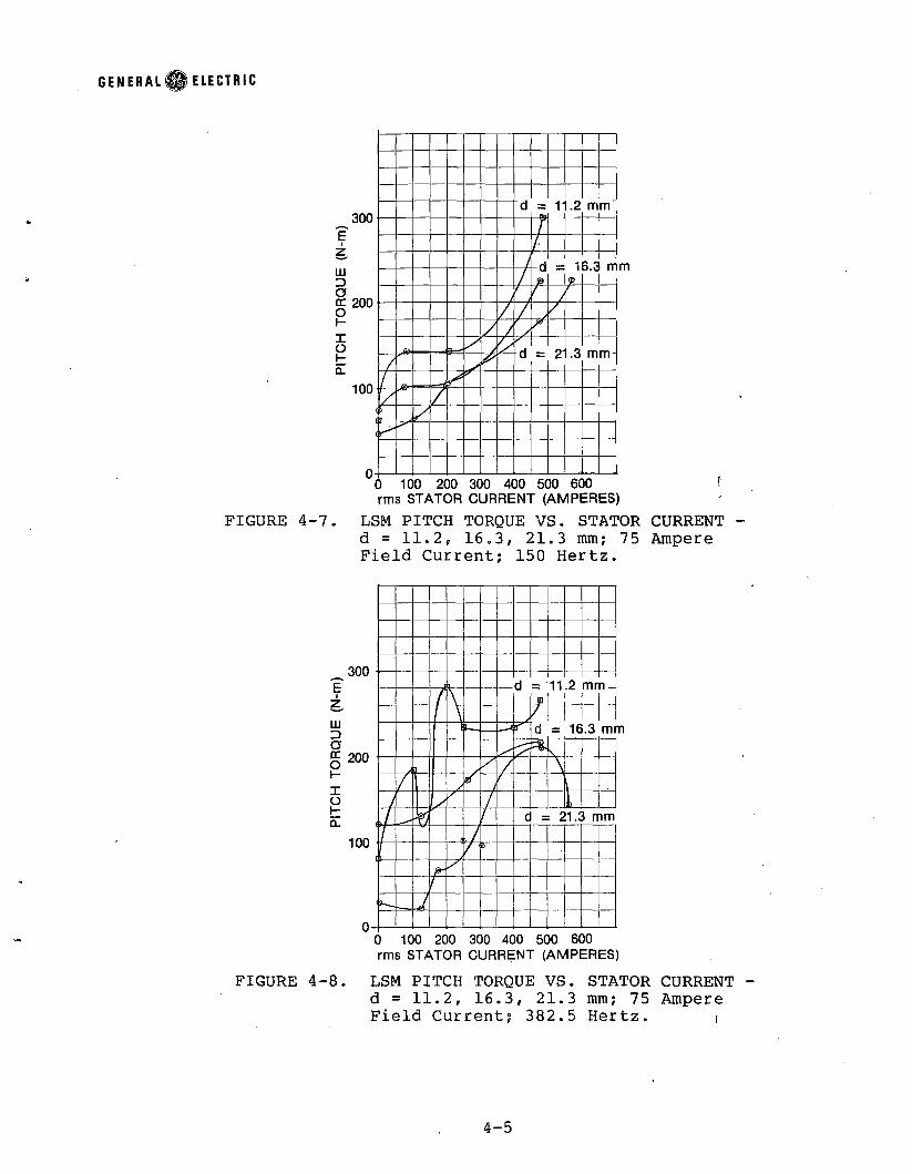
4-7 LSM Pitch Torque Vs. Stator Current - d = 11.2,16.3, 21.3 mm; 75 Ampere Field Current; 150 Hertz. . 4-54-8 LSM Pitch Torque Vs. Stator Current - d =.11.2,16.3, 21.3 mm; 75 Ampere Field Current; 382.5 Hertz. 4-54-9 LSM Efficiency and Power Factor Vs. Thrust -

d = 11.2, 16.3, 21.3 mm; 75 Ampere Field Current;60 Hertz..................... ............ .. 4-6

4-10 LSM Efficiency and Power Factor Vs. Thrust -d = 11.2, 16.3, 21.3 mm; 75 Ampere Field Current;150 Hertz......................................... 4-6

4-11 LSM Efficiency and Power Factor Vs. Thrust -d = 11.2, 15.3, 21.3 mm; 75 Ampere Field Current;382.5 Hertz........... .......................... 4-7

4-12 LSM Lateral Force Vs. Stator Current for LateralDisplacements - e=0, ±12.5, ±25 mm; 75 Ampere Field Current; 60, 150, 382.5 Hertz. ............ . 4-8

4-13 LSM Thrust Vs. Stator Current for LateralDisplacements - e=0, ±12.5 mm, ±25 mm; 75 AmpereField Current; 60 Hertz.......................... 4-8

4-14 LSM Thrust Vs. Stator Current for LateralDisplacements - e=0, ±12.5 mm, 75’Ampere FieldCurrent; 150 Hertz................... ........... 4-9

4-15 LSM Thrust Vs. Stator Current for LateralDisplacements - e=0, ±12.5 mm, ±25 mm; 75 AmpereField Current; 3 82.5 Hertz....................... 4-9

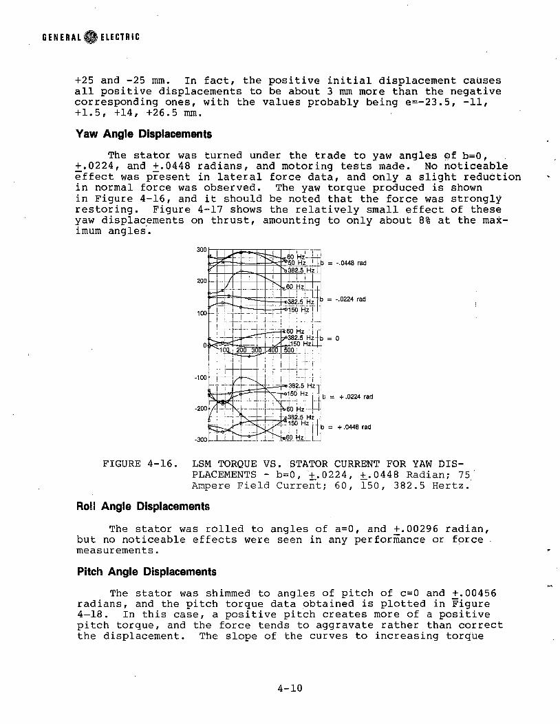
4-16 LSM Torque Vs. Stator Current for Yaw Displacements- b=0, ±.0224, ±.0448 Radian; 75 Ampere Field Current;60, 150, 382.5 Hertz............. ............... 4-10

4-17 LSM Thrust Vs. Yaw Displacement - b=0, ±.0224,±.0448 Radian, 75 Ampere Field Current; 60, 150,382.5 Hertz................... . . . . . . . . . . . 4-11

4- 18 LSM Pitch Torque Vs. Stator Current for Pitch AngleDisplacements - c=0, ±.00456 Radian; 75 Ampere Field Current; 60, 150, 382.5 Hertz. .............. . . . 4-11

5- 1 Experimental Setup for DC Force Measurements . . . . 5-25-2 Reluctance Force Vs. Distance for Homopolar LSM. . . 5-35-3 Two Positions of Saliencies Relative to Armature mmf

During Reluctance Force Measurements .............. 5-45-4a Force Vs. Distance for Homopolar L S M .......... - . . 5-55-4b LSM Laminated Track Synchronous Reactance X<j Vs.

Field Current - 382.5 Hertz, 1530 rpm......... 5-$

vii

\G E N E R A L # ELECTRIC

I

LIST O F ILLUSTRATIONS (CONT’D)a

Figure Page5-5 Homopolar LSM Waveforms for an Open Circuit to Short Circuit Step ...................................... 5-65-6 Envelopes of Phase Voltage and Current Waveforms

During Slip Test................................. 5-85-7 Phase Current Rise Times................i . . . . 5-105-8 LSM Laminated Track Search Coil Locations for Flux Measurement, Definition of Flux Components ........ 5-115-9 LSM Laminated Track Quasi-Static Flux Measurements . 5-135-10 LSM Laminated Track Flux Measurements, Flux Coil (

Near Center of Stator - 240 rpm (17.4 m/sec) . . . . 5-145-11 SLEM Static Test of Air Gap Flux - Hall Probe

Centered Over Stator Tooth ........................ 5-155-12 LSM Laminated Track Peak AC Flux Density Vs. Slot

Position - 60, 150, 382.5 Hertz................. 5-165-13 LSM Laminated Track Pole Coil Voltage............ . 5-175-14 LSM Laminated Track - Position of Track Pole Over

Stator at Interruption of Position Sensor Number 2 . 5-185-15 Track Pole Coil Voltage Vs. Time - 60 Hertz, 240 rpm,

40 Ampere Field........... . ......................... 5-195-16 Track Pole Flux Vs. Time - 60 Hertz, 240 rpm,

40 Ampere Field.......................................... 5-195-17 Track Pole Flux Vs. Time (Position) - 60 Hertz,

240 rpm, 75 Ampere Field ...........................' . . 5-205-18 Track Pole Flux Vs. Time (Position) - 150 Hertz,

600 rpm, 75 Ampere Field . . . . . ......... . . . . 5-215-19 Track Pole Flux Vs. Time (Position) - 382.5 Hertz,

1530 rpm, 75 Ampere Field. ............................. 5-216 - 1 Description of Form Factors Km and Ku.................6-26 - 2 Geometry for Calculation of Km and Ku for Varying

Gap Ratio.............................................. 6-36-3 Interarmature Flux in Homopolar Linear Synchronous

Motor and Analogy to Tooth-Tip Leakage Flux......... 6-67-1 Sample Run from a Sample Data Reduction Program. . . 7-3

yiii

LIST OF TABLES

1-1 Design Details for 155 kw Homopolar Inductor o Motor Model................................. 1-2

3-1 LSM Laminated Track Performance Adjustment ........ 3-83-2 LSM Laminated TracJc Performance Adjustments.......... 3-96- 1 Comparison Between Test Data and Original

and Revised Versions of Design Programfor 112 kW HomOpolar LSM ...................... .. . 6- 107- 1 LSM Data Channel Assignments ............ 7-2

G E N E R A L fP ELECTRIC

Table . Page

ix

G E N E R A L ® ELECTRIC

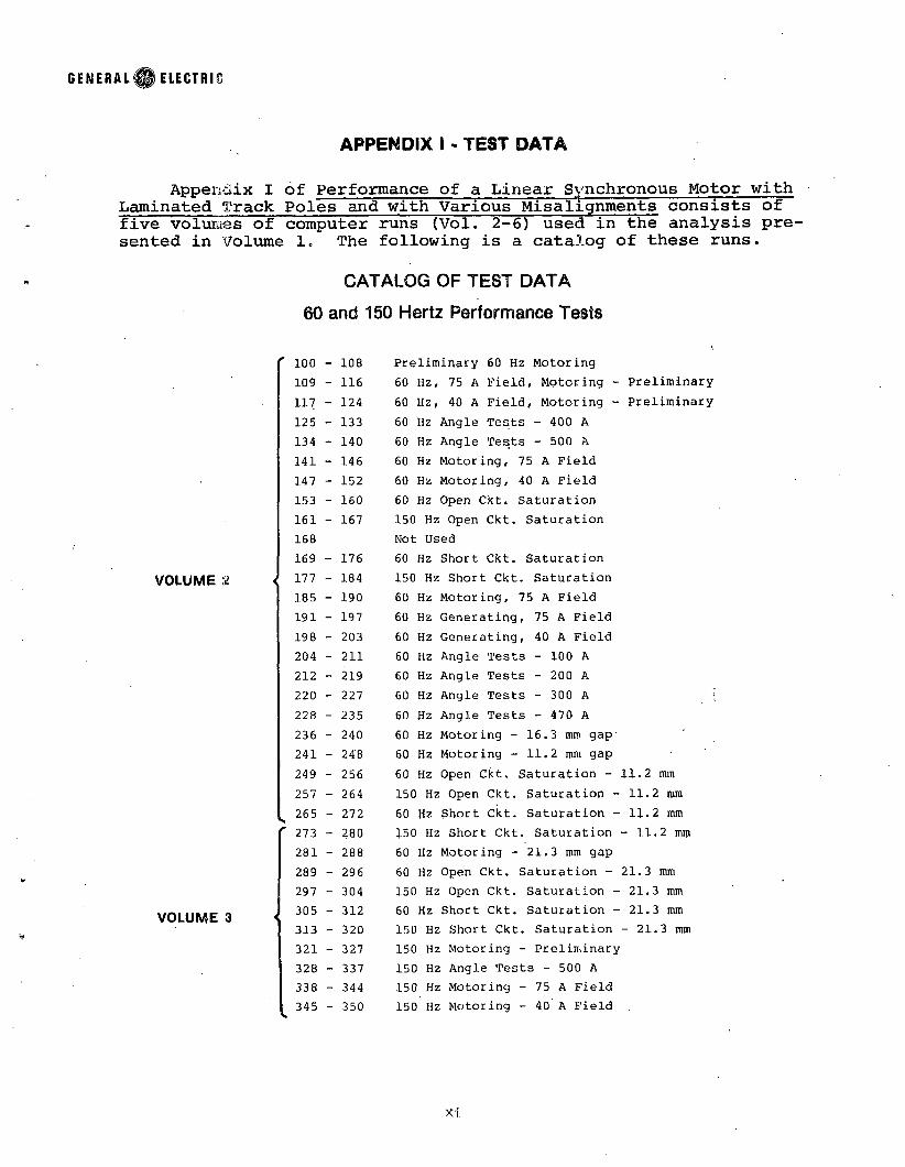
APPENDIX I • TEST DATA

Appendix I of Performance of a Linear Synchronous Motor with Laminated Track Poles and with Various Misalignments consists of five volumes of computer runs (Vol. 2-6) used in the analysis pre­sented in Volume 1. The following is a catalog of these runs.

CATALOG OF TEST DATA

60 and 150 Hertz Performance Tests

VOLUME 2

VOLUME 3

1 0 0 - 108 Preliminary 60 Hz Motoring109 - 116 60 Hz, 75 A Field, Motoring - Preliminary117 - 124 60 Hz, 40 A Field, Motoring - Preliminary125 - 133 60 Hz Angle Tests - 400 A134 - 140 60 Hz Angle Tests - 500 A141 - 146 60 Hz Motoring, 75 A Field147 - 152 60 Hz Motoring, 40 A Field153 - 160 60 Hz Open Ckt. Saturation161 - 167 150 Hz Open Ckt. Saturation168 Not Used169 - 176 60 Hz Short Ckt. Saturation177 - 184 150 Hz Short Ckt. Saturation185 - 190 60 Hz Motoring, 75 A Field191 - 197 60 Hz Generating, 75 A Field198 - 203 60 Hz Generating, 40 A Field204 - 2 1 1 60 Hz Angle Tests - 100 A2 1 2 - 219 60 Hz Angle Tests - 200 A2 2 0 - 227 60 Hz Angle Tests - 300 A •228 - 235 60 Hz Angle Tests - 470 A236 - 240 60 Hz Motoring - 16.3 mm gap'241 - 248 60 Hz Motoring - 11.2 mm gap249 - 256 60 Hz Open Ckt. Saturation - 11.2 mm257 - 264 150 Hz: Open Ckt. Saturation - 11.2 mm265 - 272 60 Hz Short Ckt. Saturation - 11.2 mm27 3 - 280 150 Hz: Short Ckt. Saturation 11.2 mm281 - 288 60 Hz Motoring - 21.3 mm gap289 - 296 60 Hz Open Ckt. Saturation - 21.3 mm297 - 304 150 Hz: Open Ckt. Saturation - 21.3 mm305 - 312 60 Hz Short Ckt. Saturation - 21.3 mm313 - 320 150 Hz; Short Ckt. Saturation - 21.3 mm321 - 327 150 Hz: Motoring - Preliminary328 - 337 150l Hz: Angle Tests - 500 A338 - 344 150l Hz: Motoring - 75 A Field345 - 350 150i Hz: Motoring - 40 A Field

xi.

G E N E R A L ® ELECTRIC

VOLUME 4

351 - 352 R u n s for D P O Data353 - 359 150 Hz G e n e r a t i n g - 40 A Fi e l d360 - 365 150 Hz G e n e r a t i n g - 75 A Fi e l d366 - 370 150 Hz M o t o r i n g - 16.3 m m gap371 - 378 150 Hz M o t o r i n g - 11.2 m m gap379 - 384 150 Hz M o t o r i n g - 21.3 m m g a p385 - 398 . 150 Hz G e n e r a t i n g - 75 A Fi e l d399 - 403 150 Hz e = o

150 Hz G - Ta b l e Tests

404 - 408 150 Hz e = o409 - 413 150 Hz e = +12.5 mm414 - 419 150 Hz e = +25 mm420 - 424 150 Hz e = 12.5 m m425 - 430 150 Hz e = 25 mm431 - 435 150 Hz e = o, f = o436 - 440 150 Hz b = +.0224 rad441 - 445 150 Hz b = +.0448 rad446 - 450 150 Hz b = -.02 2 4 rad451 - 455 150 Hz b = - . 0 4 4 8 rad456 - 460 150 Hz b 0II0II

4 61 - 465 150 Hz a = +.00148 rad466 - 470 150 Hz a = - . 0 0 1 4 8 rad471 - 475 150 Hz a = +.00 2 9 6 rad476 - 480 150 Hz a = +.00 2 9 6 rad481 - 485 150 Hz a II o o II 0

486 - 490 150 Hz c = +.00 4 5 6 rad'491 - 495 150 Hz c = - . 0 0 4 5 6 rad496 - 500 150 Hz c = o501 - 505 60 Hz e ■ ■= o

60 Hz 6 - Ta b l e Tests

506 - 510 60 Hz e = +12.55 mm511 - 516 60 Hz e = +25 mm517 - 521 60 Hz e = -1 2 . 5 m m522 - 527 60 Hz e = -25 jnm528 - 532 60 Hz e = o, b = o533 - 537 60 Hz b = +.0224538 - 542 60 Hz b = +.0448543 - 547 60 Hz b = -.0224548 - 532 60 Hz b = -.0448533 - 557 60 Hz b = o, a = o558 - 562 60 Hz z = + . 0 0296 rad563 - 567 60 Hz a = - . 0 0 2 9 6 rad568 - 572 60 Hz a = o, c = o573 - 577 60 Hz c = +.00 4 5 6 rad578 - 582 60 Hz c = - . 0 0 4 5 6 rad583 - 587 60 Hz c = o

x ii

G E N E R A L ® ELECTRIC

VOLUME 5

VOLUME 6

► 382.5 Hz P e r f o r m a n c e Te s t s588 - 590 1500 rpm F r i c t i o n W i n d a g e591 - 598 382.5 Hz O p e n C i r c u i t S a t u r a t i o n599 - 606 382.5 Hz S h o r t C i r c u i t S a t u r a t i o n607 - 609 382.5 Hz p r e l i m i n a r y M o t o r i n g Test610 - 616 382.5 Hz A n g l e T e s t s - 550 A.617 - 622 382.5 Hz A n g l e T e s t s - 550 A623 - 631 382.5 Hz M o t o r i n g , 75 A Fi e l d632 - 639 382.5 M o t o r i n g , '40 A Field640 - 644 382.5 Hz M o t o r i n g , d = 16.3 m m645 - 652 382.5 Hz M o t o r i n g , d = 21.3 mm653 - 660 382.5 Hz O p e n Ckt. S a t u r a t i o n , d = 21.3 m m661 - 668 382.5 Hz Sh o r t Ckt. S a t u r a t i o n , d = 21.3 m m669 - 676 382.5 ilz Sh o r t Ckt. S a t u r a t i o n , d = 11.2 m m677 - 684 382.5 Hz O p e n Ckt. S a t u r a t i o n d = 11.2 m m685 - 692 382.5 Hz M o t o r i n g , d = 11.2 mm

382.5 Hz G - T a b l e Te s t s -

693 - 697 382.5 Hz Runs for D P O , e = o698 - 702 382.5 Hz e = +12.5 m m703 - 708 382.5 Hz e = +25 m m709 - 713 382.5 Hz e = - 1 2 . 5 m m714 - 719 382.5 Hz e = -25 m m720 - 724 382.5 Hz e = o, b = o725 - 729 382.5 Hz b = -.02 2 4 rad730 - 734 382.5 Hz b = - . 0 4 4 8 rad735 - 739 382.5 Hz b = +.0224 rad740 - 744 382.5 Hz b = - . 0 4 4 8 rad745 - 749 382.5 Hz b = o, a = o

J 750 - 754 382.5 Hz a = + . 0 0 2 9 6 radJ 755 - 759 382.5 Hz a = - . 0 0 2 9 6

760 - 764 382.5 Hz a = o, c = o765 1530 rpm - F r i c t i o n & W i n d a g e766 - 770 382.5 Hz' c = + . 0 0 4 5 6 rad771 - 775 382.5 Hz c = - . 0 0 4 5 6 rad776 - 780 382.5 Hz c = o781 - 783 382.5 Hz M o t o r i n g , Phot o s784 t 785 382.5 Hz DPO Runs786 - 790 '382.5 Hz M o t o r i n g , 85 A Field791 - 794 382.5 Hz Rotor Flux Plots795 - 804 150 Hz U n i t y D i s p l a c e m e n t Factor805 60 Hz M o t o r i n g

xiii

GENERAL® ELECTRIC

PREFACE

This report describes and summarizes the tests run on the General Electric/Department of Transportation laminated track single-sided homopolar Linear Synchronous Machine (LSM)» These tests were part of a program to evaluate both linear induction and linear synchronous machines. In the part of the program described . in this report, the measured performance of the laminated track LSM is summarized for frequencies of 60 hertz, 150 hertz, and 383 hertz, with several different field current values and a wide range of armature currents. The measured performance under off- nominal, or G-matrix conditions, wherein the stator was displaced by various offsets and angles, is also shown. Measurements of re­luctance forces with dc armature excitation, values for the LSM equivalent circuit parameters, and flux desities are discussed, and the LSM design program modifications necessitated by poor con­dition between design and tested values are outlined.

Section 1 of this report describes the electromagnetic and mechanical design of the LSM. Section 2 describes open and short circuit tests, and Section 3 describes the performance of the ma­chine under load. Curves showing the effect of displacing the motor (G-matrix) are shown in Section 4. Section 5 discusses the measurement of equivalent circuit parameters, air gap, and pole piece flux and dc static forces. Section 6 shows the corrections which were made to the LSM design program to account for the large difference between predicted and tested behavior. The resulting design program is discussed in detail in the Phase III report. Section 7 gives an introduction to the test data and data reduction program. All the test data for this phase of the test program are listed in Appendix I, Volumes 2 through 6.

1

GENERALH ELECTRIC

Section 1INTRODUCTION AND MACHINE DESIGN SUMMARY

The model Laminated Track Homopolar Linear Synchronous Motor was built in an effort to measure the available design procedures and refine them. A round track and segment stator were chosen to suit the available test facility, described in Section 1 of the Phase II Report on the Single-sided Linear Induction Motor (SLIM). The data acquisition system described therein was used in these tests, with appropriate adjustments and re-assignments of channels. The 112 kW model was tested at low, medium, and high speeds of17.4, 43.5 and 111 meters per second, corresponding to 50, 150 and382.5 hertz operating frequencies. Power for the machine was sup­plied by a rectifier and controlled current inverter. Synchronous operation was controlled by circuits which adjusted current levels and phase relationships of the inverter supply using opto-electronic sensors on the track and analog and digital processing of command and feedback signals.ELECTROMAGNETIC DESIGN

Table 1-1 is a tabulation of the electromagnetic and related mechanical parameters of the test machine. The left column, dated 12/77, gives the characteristics and parameters of the machine as designed, while the right one, dated 4/78, gives these values as produced by the design program after it was corrected and adjusted for the actual performance of the test machine. Note that the original design was based on a 155 kW rating so as to provide oper­ating margin if performance fell short of design. Further compar­ison and explanation of these two sets of information appear in Section 6 of this report, while details of the mechanical construc­tion appear below.

1 - 1

GENERAL || ELECTRIC

TABLE 1-1. DESIGN DETAILS FOR 155 kW HOMOPOLAR INDUCTOR MOTOR MODEL

Computer Symbol Value

General 12/77 4/78Kilowatt Rating 155.00 96.00Linear Velocity, kra/hr 402.00 402.00Voltage (line to neutral) 140.00 87.00Amperes 370.00 370.00Frequency, Hz 394.30 394.30Pole Ptch, cm 14.17 14.17Per Unit Pole Arc 0.50 0.50Gap Length, cm 1.52 1.52Winding Pitch 0.833 0.833

H14Slottinq and Armature Windinq Total Slot Depth, cm 1.98 1.98

Bl = B4 Slot Width 1.27 1.27(rectangular), cm Slot Pitch, T , cm 2.36 2.36Tooth Width Wt, cm 1.09 1.09Ratio Slot Width/Slot Pitch 0.54 0.54

SLOTS Number of Slots 35.00 35.00S/P/P Slots/Pole/Phase 2 .0 0 2 .0 0

Number Pole Pairs 2.50 2.50TPC Turns/Coil 2 .0 0 2 .0 0

CIR Number Parallel Circuits 1 .0 0 1 .0 0

STR Strands of Wire 4.00 4.00T/PH Turns/Phase 2 0 .0 0 2 0 .0 0

T/PHE Effective T/PH = (T/PH)kpd 18.66 18.66WIRE Rectangular, WWB, Width, cm 0.564 0.564

HWB, Height, cm 0.183 0.1832Wire Area, cm 0.096 0.096

2Current Density, A/cm 964.00 964.00Surface Current Density, 585.00 585.00

STCW

A/cm

Weiqhts in Kiloqrams Stator Core 37.0 37.0-

YW Yoke 24.0 31.0CUACIJ Armature Copper 2 2 .0 2 2 .0

FCUW Field Copper 87.0 87.0STW Total Motor (excludes 170.0 177.0

TRWPPtrack)

Track Weight Per Pole 1 0 .0 1 0 .0

1-2

GENERAL© ELECTRIC

TABLE 1-1. DESIGN DETAILS FOR 155 kW HOMOPOLAR INDUCTOR MOTOR MODEL (CONTINUED)

Overall Lenqths (cm) 12/77 4/78HISP Stack(s) plus Field Space 25.00 25.00SPI Field Space 13.00 13.00HI Stack Length 11.95 11.95LOEDT Length Over End Turns 41.10 41.10H14 Slot Depth Total 1.98 1.98HCOR Core Depth Behind Slot 4.93 4.93HY Yoke Depth 2.17 2.82TH Total Machine Depth 9.08 9.73TLM Total Machine Length 85.00 85.00HTR Height of Track, maximum 7.62 7.62WTR Width of Track, maximum (Direction of Travel) 7.10 7.10

TPOLE Pole Pitch 14.17 14.17Motor Estimated Parameters (V=600/phase, 394 Hz)

RPH/RPU Hot Resistance ac winding fi /pu .013/.035 .013/.057XS/XSPU Leakage Reactance 0/pu .16/.43 .14/.61XAD/XADPU Direct-Axis Mutual ft/pu .15/.39 .17/.70XAQ/XAQPU Quadrature-Axis Mutual

fi /PU.12/.32 .14/.58

XF/XFP Field Leakage Si/pu .15/.388 .47/2.0XD1/XD1P Direct-Axis Transient Reactance I2/pu .24/.63 .26/1.13XC/XCP Commutating Reactance Sl/pa .26/.59 .27/1.16

Flux, Flux Densities and Field Form CoefficientsBGAP Maximum Gap Density Tesla 0.81 0.81BT Maximum Stator Tooth Density 1 .8 6 1 .8 6

BMCOR Maximum Stator Core Density 1.40 1.40BMY Maximum Yoke Density- 1.55 1.55BMTR Maximum Track Density 1.55 1.55FLDCT Total Flux, dc in airgap (weber) 0.0136 0.0156FLAC ac Flux in Airgap 0.0048 0.0032FLDCY Flux dc in frame 0.0095 0.0124KU ' (Total Flux/ac Flux) in Pole 2.82 4.83KM Maximum Flux Density/ Average Flux Density 2.03 1.75

ATF Ampere Turns Provided 2 5 , by Field ,312.0 30,515.0

Field Coil DataTURNS Field Coil Turns 336.0 336.0LAYERS Coil Sides/Width (SPI) 24.0 24.0CDF Current Density in Field Coil (A/crn ) 465.0 465.0

1-3

G E N E R A L S ELECTRIC

STATORStator Winding

The model machine has been chosen to have a five-pole wind­ing and two cores of 2.36 in. (6 cm) width. The five-pole length is dictated by the requirement of a constant number of saliencies over the stator to produce a constant reluctance in the dc circuit. Figure 1-1 shows the arrangement of the coils, the connections, and the rotor saliencies. The figure-eight winding pattern pro­vides proper phasing of stator currents for use of straight-across trade poles, simplifying the track structure appreciably.

The constraints of construction and testing of the linear synchronous machine dictated that the model be built curved, with an air gap radius of approximately 27 in. (0.686 meter). This meant that, in curving the machine, some of the linear dimensions must change. The track pole pitch of 5.58 in. (14.17 cm) was main­tained, and this necessitated an increase in the stator slot pitch from .93 (2.36 cm) to .951 in. (2.415 cm) at the air gap and .978, in. (2.48 cm) at the bottom of the slot.

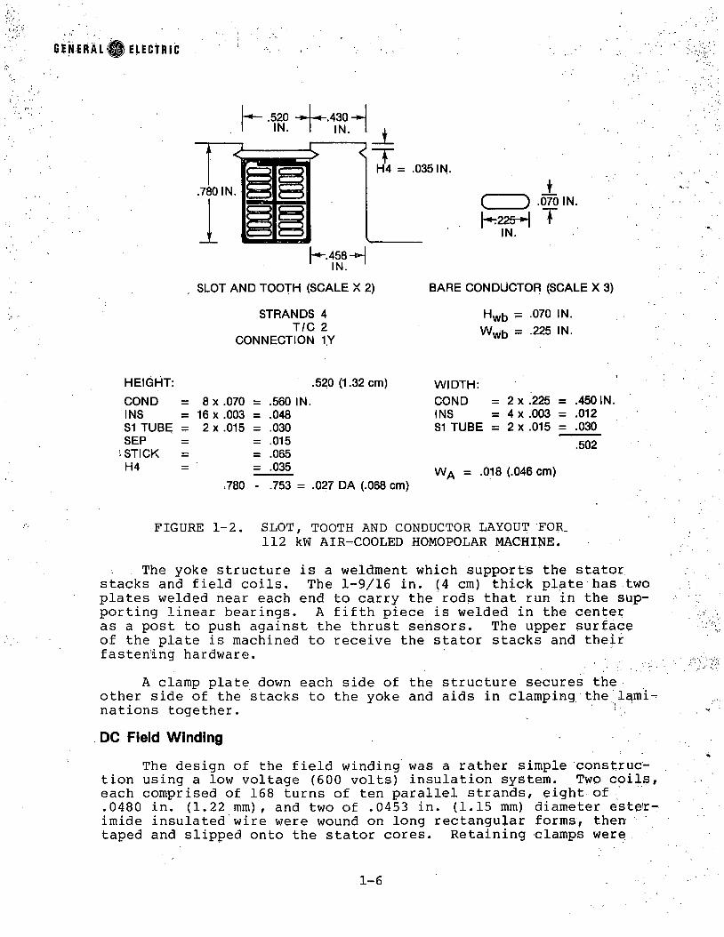
Figure 1-2 shows the slot and tooth of the machine. The tooth width at the gap is the same as. in the flat machine, so that the flux to saturate the teeth will be the same. The rectangular slot causes a slight widening of the tooth at its root.

Slot depth was held the same as in the flat machine, and the width was increased slightly, from 0.500 (1.27 cm) to 0.520 in.(1.32 cm). The dimensions of the slot allowed use of coils wound two turns per coil from four parallel wires of .070 in. x .225 in. (1.78 x 5.72 mm) copper with quadruple esterimide insulation. This wire was chosen as the most appropriate available size and insula­tion build. The insulation treatment of the coils in the slots is indicated in Figure 1-2. Although the peak voltage spikes de­livered by the inverter were expected to be only about 700 volts, a 2300 volt insulation system was used to be on the safe side.This system was based on mica-mat tape and sheet insulation and on vacuum pressure impregnation.

Stator Core ConstructionThe construction of the stator core is detailed in Figures 1-3

and 1-4. The laminations are of .014 in. (.36 mm) silicon steel, and the vendor was given the option of manufacturing each one in two pieces. The split lines for the two-piece option are shown in Figure 1-3, one slot to each side of center. Accepted motor manu­facturing standards for slot tolerances, burrs, and lineup have been applied to the lamination stacks. A total of nine bolts through each stack clamp the laminations together and hold the stacks to the steel yoke.

1-4

ELECTRIC

GENERALI ELECTRIC

C±

) .070 IN.|-*t225- J T

IN.

. SLOT AND TOOJH (SCALE X 2) BARE CONDUCTOR (SCALE X 3)STRANDS 4

T/C 2CONNECTION 1Y

H wb = .070 IN. W wb = .225 IN.

HEIGHT: .520 (1.32 cm) WIDTH:COND = 8 x .070 = .560 IN. COND = 2 x .225 = .450 ININS = 16 X .003 = .048 INS = 4 x .003 = .012S1 TUBE = 2 x .015 = .030 S1 TUBE = 2 X .015 = .030SEP = .015 .502STICK = .065H4 = .035 W A = .018 (.046 cm)

.780 - .753 = .027 DA (.068 cm)

FIGURE 1-2. SLOT, TOOTH AND CONDUCTOR LAYOUT FOR.112 kW AIR-COOLED HOMOPOLAR MACHINE.

The yoke structure is a weldment which supports the stator, stacks and field coils. The 1-9/16 in. (4 cm) thick plate has two plates welded near each end to carry the rods that run in the sup­porting linear bearings. A fifth piece is welded in the center as a post to push against the thrust sensors. The upper surface of the plate is machined to receive the stator stacks and their fastening hardware.

A clamp plate down each side of the structure secures the other side of the stacks to the yoke and aids in clamping the lami­nations together. '

DC Field WindingThe design of the field winding was a rather simple construc­

tion using a low voltage (600 volts) insulation system. Two coils, each comprised of 168 turns of ten parallel strands, eight of .0480 in. (1.22 mm), and two of .0453 in. (1.15 mm) diameter estqT- imide insulated wire were wound on long rectangular forms, then taped and slipped onto the stator cores. Retaining clamps were

1-6

GENERAL® ELECTRIC

GENERAL I I I ELECTRIC

FIGURE 1-4. STATOR AND SUPPORT ASSEMBLY.

applied, the ac winding inserted and connected, and the entire stator assembly vacuum-pressure impregnated. For operation the two-field coils were connected in series.

SYNCHRONOUS MOTOR DESIGN AND FABRICATION: ROTORFactor of Safety

The 1.35 m (53.2 in.) diameter rotor has a top rated speed of 1530 rpm for 111 m/sec (250 miles per hour). At this speed the- centrifugal "g" force on the outer surface is 1850, i.e., each pound on the surface has nearly a ton of centrifugal force on it. This produces stresses high enough to require care in design, but not so high that normally available materials cannot be used.

DesignThe design of the rotor is shown in Figures 1-5 and 1-6. The

two outer stacks of laminations with pole projections and the in­ner stack are made of 20 gage (0.0359 in.) cold-rolled sheet steel

1-8

G E N E R A L ® ELECTRIC

FIGURE 1-5. ROTOR DESIGN FOR THE SYNCHRONOUS MOTOR.

The flux in the outer sections must build up as the rotor passes over the field coil, at a rate dictated by the time constant.With the few number of stator poles of the sample, this reduction of flux can be large. To reduce the time constant, the pole pro­jection and yoke section are "core plated" (interlaminar insu­lated) for a depth of 1 pole pitch, which is the outside diameter of the center stack. Below this diameter the flux pulsation was expected to be "averaged out" to a low enough value to not affect buildup time, and the laminations in all three stacks are unin­sulated, to reduce the interlamination "air gap" where the flux is taken "across the grain."

1 - 9

GENERAL ELECTRIC

FIGURE 1-6. ROTOR DESIGN FOR THE SYNCHRONOUS MOTOR (CONTINUED),.

In this design the rotor laminations are centered but not supported by the shaft, and at standstill have a 1 to 3 mils clear ance. The stacks are held and driven by the eight through-bolts through the shoulder on the shaft on one end and the keyed ring on the other. ' .

The outer tie bolts are insulated through the. stacks so thatthe laminations will not be shorted.

1-10

GENERAL ELECTRIC

Sesttosi 2

OPEN CIRCUIT AND SHORT CIRCUIT TESTS

This section describes and presents the results of tests of friction and windage, open circuit saturation and short circuit saturation tests on the laminated track machine.

FRICTION AND W INDAG E CORRECTIONS

The LSM was driven by the dc load motor at speeds near 240 rpm (60 hertz synchronous speed) and 600 rpm (150 hertz synchronous speed). The range of torque displayed by the torque transducer amplifier was plotted in Figure 2-1. A reasonably smooth curve was put through these torque ranges, and the square root, labeled / x , was plotted. A reasonable fit to the data was obtained as

vT = .0117 x rpm +0.9,

or t = .0001369 x rpm2 + .0211 x rpm + .81 (2-1)

and this relationship was used as the friction and windage contri­bution in all calculations of performance at 60 and 150 hertz.This contribution was added to the measured shaft torque for all motoring data and subtracted from the shaft torque for generating data, open circuit, and short circuit curves.

At full speed, the relationship of torque to speed was not exactly reflected by the expression developed for lower speeds. A new set of data was taken near 1530 rpm (382.5 hertz synchronous speed), and the results of this test are shown in Figure 2-2. The dashed line is the relationship

= .0001324 x rpm2, (2-2)

which was used as a simple correction in all performance data at382.5 hertz.

OPEN CIRCUIT VOLTAGE AND LOSSES

The first test was to use the dc motor to drive the machine at 240 rpm (17.4 mps) with field applied and the ac terminals.open* Figure 2-3 shows the three 60 hertz line-to-neutral voltages ob­tained with a 75 A field current. The voltages are quite sinu­soidal, showing very little harmonic content, and appear in phase sequence C-B-A. The five-pole connection of the ac winding was used in this test, as in all subsequent tests presented here. The open cirucit voltage produced by the machine was 13.2 volts rms, measured by digital voltmeter, and the scope traces agree as nearly as can be measured.

The field current was varied in order to produce the open cir­cuit saturation curve shown in Figure 2-4. Again, the speed was

2-1

G E N E R A L S ELECTRIC

S P E E D ( r p m )

FIGURE 2-1. LSM LAMINATED TRACK FRICTION AND WINDAGE TORQUE VS. SPEED NEAR 240 AND 600 rpm OPERATING CONDITIONS.

FIGURE 2-2. LSM LAMINATED TRACK FRICTION AND WINDAGE TORQUE VS. SPEED NEAR 1530 rpm OPERATING CONDITIONS.

2-2

I.

FIGURE 2-3. LSM LAMINATED TRACK LINE-TO-NEUTRAL VOLTAGES AT 75 AMPERE FIELD - 240 rpm (12.4 mps), 60 Hertz.

240 rpm to produce 60 hertz output. The shape of the saturation curve produced for this machine differs from that of a conventional synchronous machine, as can be seen in the decreased voltage output at high field currents. The output voltage increases linearly with field current from zero to about 30 A, then begins to show satura­tion. At about 87 A, the voltage actually starts to decrease for increasing field current. Saturation of either the stator teeth, the track saliencies, or both, apparently causes the effective alternating component of flux in the air gap to decrease. The ratio of the gap between saliencies to the gap over saliencies decreases, resulting in this reduction of flux variation. In this case, the maximum measured output voltage with the nominal air gap of 16.3 mm was 13.33 volts, at about 87 A field. The curves for the increased air gap of 21.3 mm and for the decreased gap of 11.2 mm show the inverse nature of variation of voltage with gap dimension. While the magnitude of open circuit voltage changes with air,, gap, the shape of the excitation curve remains very similar.

Figure 2-5 shows the mechanical (shaft) input (less friction and windage) to the machine as a function of field current and gap dimension. The point-to-point variation in this data is the re­sult of limitations in the speed control loop and the torque trans­ducer's resolution. These curves represent the magnetic losses in the stator and track associated with the buildup and decay of flux in the track poles and the alternating component of flux seen in the stator core as track poles pass over it. For the nom­inal gap at 75 A field, this amounts to about 440 watts, or about 2.5% of machine rating at this speed. These losses vary generally upward with decreasing air gap, downward with increasing gap.

2-3

G E N E R A L ® ELECTRIC

FIGURE 2-4. LSM LAMINATED TRACK OPEN CIRCUIT VOLTAGE VS.FIELD CURRENT AND AIR GAP - 60 Hertz, 240 rpm; g = 11.2, 16, 3, 21.3 mm.

Figures 2-6 and 2-7 show the open circuit voltage and magnetic losses as obtained at 150 hertz. The maximum voltage obtained with the nominal air gap was 34.0 volts, just 2.5 times the volt­age at 60 hertz. Within the limitations of measurement of speed, field current and terminal voltage, the machine displayed a con­stant volts-per-hertz characteristic. The magnetic losses at nom­inal gap and 75 A field were about 2100 watts, 4.8 times those at 60 hertz, indicating a variation with (speed)1*7.

Tests of open circuit characteristics at 382.5 hertz are pre­sented in Figures 2-8 and 2-9. The maximum open circuit voltage at the nominal air gap was 86.4, within 1-1/2% of the constant volts per-hertz relationship. This error is well within the limits of speed, field current and terminal voltage measurements. Magnetic losses at 75 A field were about 7000 watts, giving a relationship of (speed) * when compared to the 60 hertz measurements. The scatter in data observed in Figure 2-9 is the result of difficulty in stabilizing the dc motor speed at the weak field required to run this fast. This difficulty appears as an oscillation in shaft torque at this high speed, but. its effects were limited to 2 or 3% of rated thrust, further reduced by attempting to take data in the center of the band of variation of shaft torque.

2-4

G E N E R A L ® ELECTRIC

0 20 40 60 80 100FIELD C U R R E N T (AMPERES)

FIGURE 2-5. LSM LAMINATED TRACK MAGNETIC LOSS VS. FIELD CURRENT AND AIR GAP - 60 Hertz, 240 rpm; d = 11.2, 16.3, 21.3 mm.

FIELD C U R R E N T (AMPERES) !FIGURE 2-6. LSM LAMINATED TRACK OPEN CIRCUIT VOLTAGE VS.FIELD CURRENT AND AIR GAP - 150 Hertz, 600 rpm

d = 11.2, 16.3, 21.3 mm.

2-5

GENERAL ELECTRIC

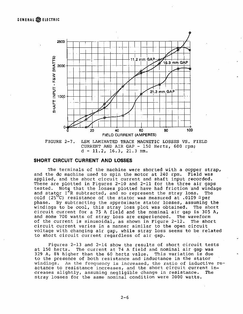
FIGURE 2-7. LSM LAMINATED TRACK MAGNETIC LOSSES VS. FIELD CURRENT AND AIR GAP - 150 Hertz, 600 rpm; d = 11.2, 16.3, 21.3 mm.

SHORT CIRCUIT CURRENT AND LOSSESThe terminals of the machine were shorted with a copper strap,

and the dc machine used to spin the motor at 240 rpm. Field was applied, and the short circuit current and shaft input recorded. These are plotted in Figures 2-10 and 2-11 for the three air gaps tested. Note that the losses plotted have had friction and windage and stator I^R subtracted, and so represent the stray loss. The cold (25°C) resistance of the stator was measured at .0109 fiper phase. By subtracting the approximate stator losses, assuming the windings to be cool, this stray loss plot was obtained. The short circuit current for a 75 A field and the nominal air gap is 305 A, and some 700 watts of stray loss are experienced. The waveform of the current is sinusoidal, as shown in Figure 2-12. The short circuit current varies in a manner similar to the open circuit voltage with changing air gap, while stray loss seems to be related to short circuit current regardless of air gap.

Figures 2-13 and 2-14 show the results of short circuit tests at 150 hertz. The current at 74 A field and nominal air gap was 329 A, 8% higher than the 60 hertz value. This variation is due to the presence of both resistance and inductance in the stator windings. As the frequency is increased, the ratio of inductive re actance to resistance increases, and the short circuit current in­creases slightly, assuming negligible change in resistance. The stray losses for the same nominal condition were 2000 watts.

2-6

G E N E R A L I ELECTRIC

FIGURE 2-8. LSM LAMINATED TRACK OPEN CIRCUIT VOLTAGE VS.FIELD CURRENT AND AIR GAP - 382.5 Hertz,1530 rpm; d = 11.2, 16.3, 2.13 mm.

FIGURE 2-9. LSM LAMINATED TRACK MAGNETIC LOSSES VS. FIELDCURRENT AND AIR GAP - 382.5 Hertz, 1530 rpm;d = 11.2, 16.3, 21.3 mm.

2-7

G E N E R A L ® ELECTRIC

FIGURE 2-10. LSM LAMINATED TRACK SHORT CIRCUIT CURRENT VS.FIELD CURRENT AND AIR GAP - 60 Hertz, 240 rpm; d = 11.2, 16.3, 21.3 mm.

FIGURE 2-11. LSM LAMINATED TRACK STRAY LOSS VS. SHORT CIRCUITCURRENT AND AIR GAP - 60 Hertz, 240 rpm;d = 11.2, 16.3, 21.3 mm.

2-8

G E N E R A L ® ELECTRIC

75 A Field

431 A

T ”(305 A rms)

90 A Field

FIGURE 2-12. LSM - LAMINATED TRACK SHORT CIRCUIT CURRENT AT 240 rpm (17.4 m/sec).

FIGURE 2-13. LSM LAMINATED TRACK SHORT CIRCUIT CURRENTVS. FIELD CURRENT AND AIR GAP - 150 Hertz,600 rpm; d = 11.2, 16.3, 21 mm.

2-9

G E N E R A L ® ELECTRIC

FIGURE 2-14. LSM LAMINATED TRACK STRAY LOSS VS. SHORT CIRCUIT CURRENT AND AIR GAP - 150 Hertz,600 rpm; d = 11.2, 16.3, 21.3 mm.

When the speed was increased to 1530 rpm (382.5 hertz) , the short circuit current increased only very slightly from the 150 hertz case. The 75 A, nominal gap value was 330 A, essentially the same as at 150 hertz. The stray losses at this current and speed are about 9000 watts, or about 8% of the machine rating. Figures 2-15 and 2-16 show these results. It should be remembered that all of. these |tray loss figures are based on a cool stator with its minimum I^R loss, and may be higher than the actual stray loss. Runs were taken rapidly, using an initially cool machine, so that these assumptions should be fairly accurate.

2-10

G E N E R A L ® ELECTRIC

FIGURE 2-15. LSM LAMINATED TRACK SHORT CIRCUIT CURRENT VS.FIELD CURRENT AND AIR GAP - 382.5 Hertz,1530 rpm; d = 11.2, 16.3, 21.3 mm.

S H O R T CIRCUIT C U R R E N T (AMPERES)

FIGURE 2-16. LSM LAMINATED TRACK STRAY LOSS VS. SHORTCIRCUIT CURRENT AND AIR GAP 382.5 Hertz,1530 rpm; d = 11.2, 16.3, 21.3 mm.

2-11

G E N E R A L ® ELECTRIC

Sesti&n 3

M ACHINE PERFORMANCE UNDER LOAD

In this section the motoring and generating performance are described in detail, including thrust, normal force, efficiency and power factor information. The operation of the inverter con­trol system is also described in so far as it affects the motor performance. All testing was performed with the dc load machine in a speed control loop and the LSM under current control.

MOTORING PERFORMANCE

After initial tests of the inverter, control, and LSM, an investigation of motor output versus inverter firing angle was undgrtaken. The control was adjusted so that the center of the 120 inverter firing pulse was from 0 to 64° ahead of the peak of the motor internal, or open circuit, voltage. This resulted in a set o£ firing pulses whose fundamental component varied from a 0 to 64 phase angle leading the internal voltage, which was the full range available from the control in the motoring mode. Fig­ure 3-1 shows the thrust produced by the motor at 60 hertz with a 75 A field and rms stator currents from 100 to 500 A. These curves show a strong peak in thrust around 20 degrees of advance for currents of 400 to 500 A, and also indicate a current of about 470 A should produce the rated thrust of 1009 newtons at approxi­mately this angle.

FIGURE 3-1. LSM LAMINATED TRACK THRUST ' VS. FIRING ANGLE - 100-500 rms Armature Amperes, 75 Am­peres Field Current, 60 Hertz.

3-1

GENERAL I p ELECTRIC

The inverter control circuitry was checked for drift, read­justed, and the curves of thrust versus firing angle with frequency as a parameter were obtained and are shown in Figure 3-2. The ma­chine produced thrust exceeding the rated 1009 newtons for rms cur­rents of 470 A at all three frequencies, corresponding to operation at 17.4, 43.5, and 111 meters per second. All subsequent tests reported here were performed with the inverter controls set for the maximum thrust per ampere as shown in Figure 3-2.

INVERTER FIRING A N G L E (DEG.)

FIGURE 3-2. LSM LAMINATED TRACK THRUST VS. FIRING ANGLE - 75 Am­peres Field Current; 60,150, 382.5 Hertz.

The thrust produced by the machine as a function of stator current at 75 A field excitation and for the three testing frequen­cies is shown in Figure 3-3. As would be expected, thrust is a linear function of current within the measurement errors of the tests, and rated thrust is produced at 465 to 470 rms A for all three test frequencies. If the machine had significant end effect,, the thrust for a given current would be expected to decrease at ■ higher frequencies, but no such effect is observed in this lami­nated track machine. The thrust curve for full-speed operation deviates from the others at light loads, probably as a result of the difficulty of measuring thrust which is significantly less than the windage force encountered. Friction and windage at 1530 rpm amounted to about 310 newton meters of torque, or 447 newtons of thrust, nearly half of the machine rating.

3 - 2

G E N E R A L ® ELECTRIC

rms STATOR CURRENT (AMPERES)FIGURE 3-3. LSM LAMINATED TRACK THRUST VS. STATOR

CURRENT - 75 Amperes Field Current;60, 150, 382.5 Hertz.

The force of attraction between the stator and the track for a 75 A field was approximately 7000 newtons, or seven times rated thrust. The curves of Figure 3-4 show the effect of armature cur­rent on the normal force. The attraction increased at low currents, then decreased at higher currents as the angle and magnitude of armature reaction flux decreased the total air gap flux. It should be noted, however, that the effect of armature reacticn is small compared to the total force.

Figures 3-5 and 3-6 show the same type of results for thrust and normal force at 40 A field excitation. The thrust produced at 470 A of stator current was 800 newtons, and the normal force was about 3500 newtons. The value of 40 A was chosen for field current as the upper end of the linear region of operation for the machine. In the 9th Quarterly Report1 it was noted that saturation appeared in the open circuit voltage of the machine for field cur­rents exceeding 40 A.

Efficiency and power factor data as calculated using the data acquisition system information, are presented in Figures 3-7 and 3-8. Note that these are plotted against thrust, not current. The efficiency results are higher than expected, a result which also appeared in the induction motor tests. The problem appears to be in the watts calculation in the hardware of the data acquisition system. Several attacks were made on this, including calculation of input power by point-by-point analysis of voltage and current waveforms usng a digital processing oscilloscope (DPO), segregation of losses, and estimation of the input power from the inverter dc link power.

1SLEM Program, 9th Quarterly Report, DOT-FR64147.

3-3

G E N E R A L ® ELECTRIC

FIGURE 3-4. LSM LAMINATED TRACK NORMAL FORCE VS. STATOR CURRENT - 75 Amperes Field Current; 60, 150, 382.5 Hertz.

0 100 200 300 400 500rms STATOR CURRENT (AMPERES)

FIGURE 3-5. LSM LAMINATED TRACK THRUST VS. STATORCURRENT - 40 Amperes Field Current; 60, 150, 382.5 Hertz.

3-4

GENERAL ELECTRIC

FIGURE 3-6. LSM LAMINATED TRACK NORMAL FORCE VS.STATOR CURRENT - 40 Amperes Field Cur­rent; 60, 150, 382.5 Hertz.

The machine was run at rated load and rated speed, and the waveforms of terminal voltage and phase current simultaneously re­corded with the digital processing oscilloscope. Figure 3-9 shows the recorded voltage waveform, and Figure 3-10 shows the current waveform. The nature of the waveforms, a slight jitter from cycle to cycle, and the scanning rate resulted in some small jumps in the recorded traces. These did not appear to make significant dif­ferences in the resulting power calculations. The harmonic analy­sis of each waveform as calculated by the DPO is presented in Fig­ures 3-11, 3-12 and 3-13, and the point-by-point calculation of power appears in Figure 3-14. The figure of 129.12 kW is based on the assumption of balanced three-phase conditions. Tests con­ducted on a phase-by-phase basis were used to produce an average power input figure to attempt to compensate for load oscillation and sampling rate limitations. The average power input over the three phases and several runs at the same load conditions was136.9 kW, for an output of 111.0 kW, so that the calculated effi­ciency is 81%. This input is some 20% higher than the 114 kW in­dicated by the data acquisition system. The nature of the DPO sampling scheme is to broaden peaks and overemphasize the width of spikes, so that the 136.9 kW may be greater than the actual input. The results of other runs at 60 and 150 hertz.showed the DPO to calculate inputs 7 and 12% higher, respectively, than the data acquisition system. These two methods of measurement, neither of them completely accurate, served to put a range on the electri­cal input and efficiency.

3- 5

GENERAL H H ELECTRIC

FIGURE 3-7. LSM LAMINATED TRACK EFFI­CIENCY AND POWER FACTOR VS. THRUST - 75 Ampere Field Current; 60, 150,382.5 Hertz.

In an attempt to order the confusion concerning power mea­surement, a segregation of the losses for operation of the motor over the range of thrusts, frequencies, and field currents tested was undertaken. The magnetic loss for the field, the stator l^R loss, adjusted for temperature of the windings, and the mechanical output were summed. This was subtracted from the electrical input provided by the data acquistion system and found to produce a neg­ative stray loss figure. The input was increased by some percen­tage, and the difference taken again. The most satisfactory stray loss figures, compared to those obtained with the machine short circuited, were then used to select the most suitable percentage to add to the data acquisition system input. The results of this calculation for low-speed operation, 60 hertz, with a 40 A and a 75 A field current are shown in Table 3-1. The electrical input was increased by 4% to obtain the most reasonable distribution of losses for the range of test points taken. This same procedure was performed on 150 hertz and 382.5 hertz data, with results as tabulated in the remainder of Table 3-1.

3-6

G E N E R A L © ELECTRIC

FIGURE 3-8. LSM LAMINATED TRACK EFFI­CIENCY AND POWER FACTOR VS. THRUST - 40 Ampere Field Current; 60, 150,382.5 Hertz.

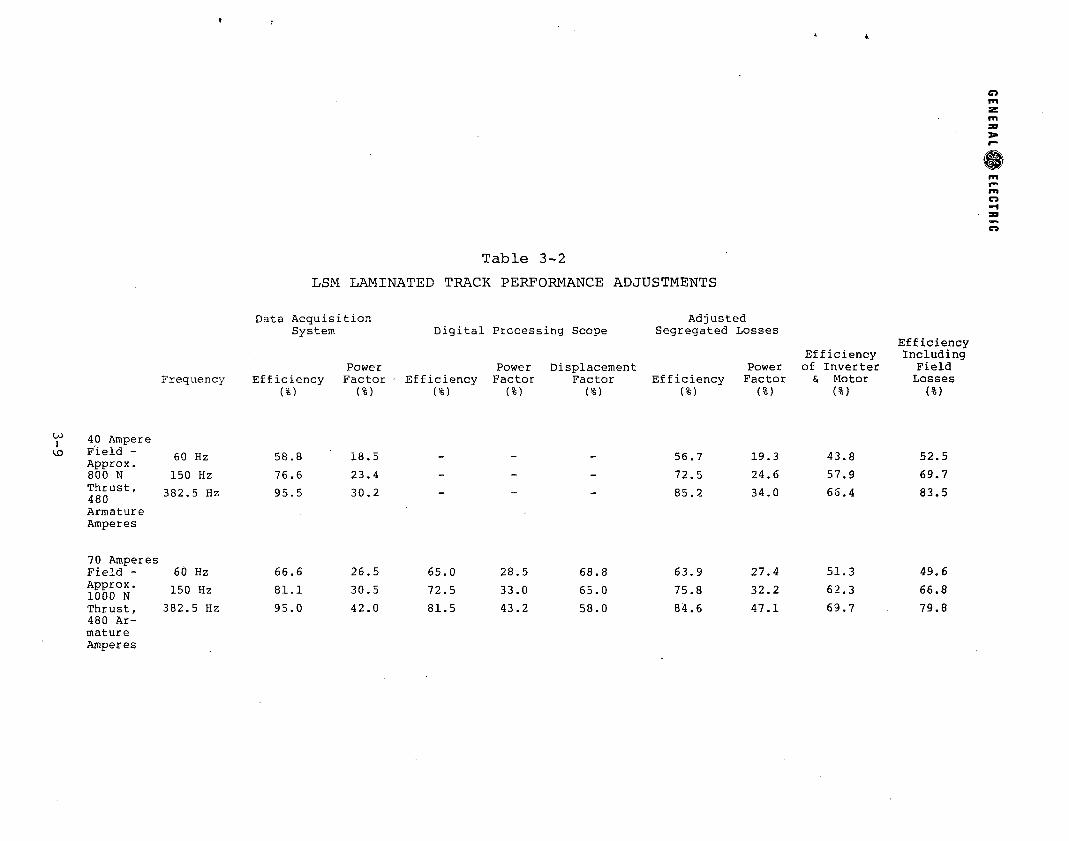
Table 3-2 summarizes the efficiency, power factor and displace­ment factor data obtained by the various methods discussed above, as well as the efficiency calculated for the combined inverter and motor. This figure was obtained from the average power in the dc link, as measured by the data acquistion system. Comparison of the combined efficiency figure to the motor efficiency shows the inverter efficiency to be approximately 79% for the 40 A field runs and 81% for the 75 A field runs. The column headed "Displacement Factor" gives the cosine of the angle between the fundamental com­ponents of voltage and current as calculated by the DPO.

C O M M U T A T I O N D E L A Y

In Figures 3-1 and 3-2, machine motoring performance was plotted as a function of inverter firing angle. If there were no commutation delay in the operation of the inverter, this angle would be the electrical angle by which the phase current leads the machine's internal voltage. Investigation of the performance of the inverter,

3-7

GENERAL | | p ELECTRIC

Table 3-1LSM LAMINATED TRACK PERFORMANCE ADJUSTMENT

60Hertz, 240rpmS tator Efficiency PowerRun Armature Input Output Magnetic Stray Estimates FactorNo. Amperes Volts kW kW Loss IR Loss % %

40 Ampere 147 97.8 20.12 3.17 2.63 0.2 0.3 0.04 83.0 53.7Field'(Input Adjusted by 148 152.2 27.65 5.38 4.34 0.2 0.8 0.04 80.7 42.6+ 4%) 149 201.7 39.60 7.68 5.88 0.2 1.4 0.20 76.6 32.1150 302.6 56.40 13.18 9.07 0.2 3.3 0.61 68.8 38.0151 401.2 77.15 19.44 11.91 0.2 6.0 1.33 61.3 20.9152 472.4 89.84 24.59 13.95 0.2 9.5 0.94 56.7 19.3(52.5 with 2 kwFieldLoss)141 91.3 21. 3 3.47 2.86 0.45 0.3 -0.14 82.4 59.5

75 Ampere 142 153.5 27.3 6.61 5.40 0.45 0.8 -0.04 81.7 52.6Field (Input 143 201.4 33.86 9.16 7.21 0.45 1.4 +0.10 78.7. 44.8Adjusted by +4%) 144 302.0 51.40 15.28 11.31 0.45 3.3 +0.22 74.0 32.8145 399.1 69.30 22.15 15.08 0.45 6.0 +0.62 68.1 26.7146 469.6 71.67 27.71 17.72 0.45 9.5 +0.04 63.9 27.4(49.6 with 8 kWFieldLoss)150Hertz, 60Ci rpm

Stator Efficiency PowerRun Armature Input Output Magnetic 2 Stray Estimates FactorNo. Amperes Volts kW kw Loss IZR Loss % %345 99.7 44.6 6.08 5.26 1.0 0.3 -0.48 86.5 45.540 Ampere 346 202.0 67.62 15.77 13.25 1.0 1.4 0.05 84.4 38.5Field (Input 347 299.1 90.84 26.90 21.61 1.0 3.2 1.09 80.3 33.0Adjusted by +6%) 348 402.9 118.9 39.82 30.28 1.0 6.0 2.54 76.0 27.7349 482.5 141.1 50.17 36.38 1.0 9.5 3.29 72.5 24.6350 0 0 0 (-0.52) 1.0 0 0 (69.7 with 2 kwFieldLoss)

338 0 ■ 0 0 -0.36 0 0 +0.36 0 0339 0 34.75 0 -1.40 2.0 0 -0.6075 Ampere 340 10 3.0 48.76 7.88 5.71 2.0 0.4 -0,23 73.2 52.2Field (Input Adjusted by 341 200.6 66.62 18.86 15.32 2.0 1.4 +0.14 81.2 47.0+6%) 342 297.3 86.10 31.70 25.70 2.0 3.2 +0.80 81.1 41.3343 398.8 108.40 46.74 36.70 2.0 5.9 2.14 78.5 36.0344 479.1 127.50 58.99 44.74 2.0 9.5 2.75 75.8 32.2(66.8 with 8 kWFieldLoss)382.5 Hertz, 1530 rpm

Stator Efficiency PowerFun Armature Input Output Magnetic 2 Stray Estimates FactorNo. Amperes Volts kW kw Loss I R Loss % %632 0 0 0 0 0 0 0 - -

40 Ampere 633 0 0 -3.0 3.0 0 0 - -Field (Input 634 100.4 100.9 6.1 1.9 3.0 0.4 0.8 31.1 20.0Adjusted by +12%) 635 205.5 133.0 34.9 30.0 3.0 1.5 0.4 86.0 42.5636 296.4 159.8 62.5 53.2 3.0 3.5 2.8 85.1 44.0637 401.2 190.5 89.5 76.8 3.0 6.7 3.0 85.8 39.0.638 478.1 215.9 105.2 89.6 3.0 10.0 2.6 85.2 34.0(83.5 with 2 kWFieldLoss)623 0 0 0 0 0 0 0 0624 0 0 -8.0 8.0 0 0 0 075 Ampere 625 82.0 108.8 1.6 -9.1 8.0 0.2 2.5 - 6.0Field (Input Adjusted by 626 100.8 114.8 3.9 -2.4 8.0 0.3 2.0 - 11.2+12%) 627 155.4 127.7 23.4 15.9 8.0 0.8 -1.3 67.9 39.3628 198.6 137.8 38.8 29.5 8.0 1.3 0 76.0 47.3629 292.5 158.9 72.0 61.1 8.0 2.8 0.1 84.9 51.6630 394.8 180.4 109.0 94.3 8.0 6.1 0.6 86.5 51.0631 473.9 198.8 133.2 112.7 8.0 9.9 2.6 84.6 47.1(79.8 with 8 kW Field Loss)

3-8

k

Table 3-2LSM LAMINATED TRACK PERFORMANCE ADJUSTMENTS

u>ikO

Data Acquisition System Digital Processing Scope

AdjustedSegregated Losses

Power Power Displacement PowerEfficiency of Inverter

EfficiencyIncluding

FieldFrequency Efficiency

(%)Factor • (%)

Efficiency(%)

Factor(%)

Factor(%)

Efficiency(%)

Factor(%)

& Motor (%)

Losses(%)

40 AmpereField - Approx. 60 Hz 58.8 18.5 - - - 56.7 19.3 43.8 52.5800 N 150 Hz 76.6 23.4 ~ - 72.5 24.6 57.9 69.7Thrust, 480ArmatureAmperes

382.5 Hz 95.5 30.2 85.2 34.0 66.4 83.5

70 AmperesField - 60 Hz 66.6 26.5 65.0 28.5 68.8 63.9 27.4 51.3 49.6Approx. 1000 N 150 Hz 81.1 30.5 72.5 33.0 65.0 75.8 32.2 62.3 66.8Thrust, 480 Ar­mature Amperes

382.5 Hz 95.0 42.0 81.5 43.2 58.0 84.6 47.1 69.7 79.8

GENERAL® ELECTRIC

GENERAL ELECTRIC

MA2878.1. UOLTS

FIGURE 3-9. LSM LAMINATED TRACK LINE-TO-NEUTRAL VOLTS - Rated Load, 382.5 Hertz.

MA2878.2

IE 3 AMPS

FIGURE 3-10. LSM LAMINATED TRACK PHASE CURRENTRated Load, 382.5 Hertz.

3-10

G E N E R A L ® ELECTRIC

HOLTS SEC

FIGURE 3-11. LSM LAMINATED TRACK LINE-TO-NEUTRAL VOLTS - Rated Load, 382.5 Hertz.

ftMFS SEC

FIGURE 3-12. LSM LAMINATED TRACK PHASE CURRENT -Rated Load, 382.5 Hertz.

3-11

GENERAL £ ELECTRIC

FILE NAME MA2878.1WAUEFORM ASCALE FACTOR= 100UNITS UOLTSHARMONIC AMPLITUOElRMSJ PHASE( degrees1 130.325 -50.8652TJ 15.3233 21 9967cr, 84.1344 124.854-91 73.574 112.947$r 4.57557 7.04387ii 32 4388 -118 74613 22.7228 174.508RMS IJALUE 202 451ANOTHER WAUEFORM ENTER 1'FILE NAME MA2878.2WAUEFORM BSCALE FACTOR:* 2020.2UNITS AMPSHARMONIC AMPLITUDE(RMS> phase< degrees1 482.734 -101.0123 9 96369 179.0865 99.3791 42.85661’ 38.5738 42.3529Cl 10.1018 166.835ii 25.3393 171.45413 6.59775 176.969RMS UALUE 497.838

FIGURE 3-13. LSM LAMINATED TRACK VOLTAGEAND CURRENT HARMONICS - Rated Load, 382.5 Hertz.

AVERAGE POWER 129190 WATTS MA2878.1 MAZ878.2IE 3 UOLTSAMPS

FIGURE 3-14. LSM LAMINATED TRACK WATTS INPUTRated Load, 382.5 Hertz.

3-12

G E N E R A L © ELECTRIC

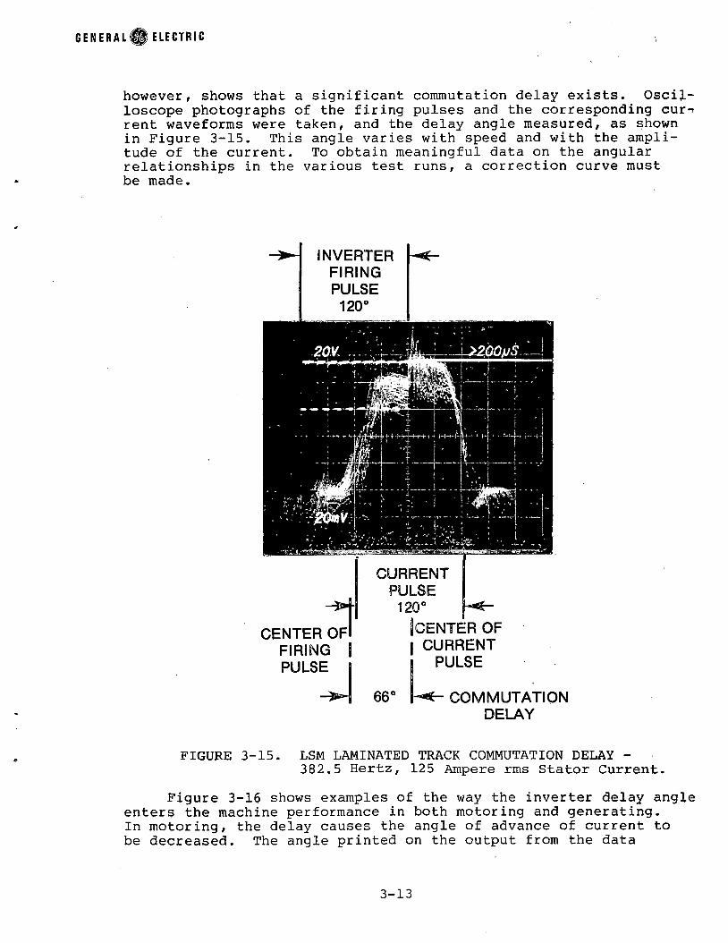
however, shows that a significant commutation delay exists. Oscil­loscope photographs of the firing pulses and the corresponding cur^ rent waveforms were taken, and the delay angle measured, as shown in Figure 3-15. This angle varies with speed and with the ampli­tude of the current. To obtain meaningful data on the angular relationships in the various test runs, a correction curve must be made.

INVERTERFIRINGPULSE120°

3 *CENTER OF FIRING PULSE

CURRENT PULSE

1 2 0 °jCENTER OF | CURRENT

PULSE

LI - U COMMUTATIONDELAY

FIGURE 3-15. LSM LAMINATED TRACK COMMUTATION DELAY -382.5 Hertz, 125 Ampere rms Stator Current.

Figure 3-16 shows examples of the way the inverter delay angle enters the machine performance in both motoring and generating.In motoring, the delay causes the angle of advance of current to be decreased. The angle printed on the output from the data

3-13

G E N E R A L ® ELECTRIC

I N V E R T E RF I R I N GP U L S E

I N V E R T E RC O M M U T A T I O N

D E L A Y

FIGURE 3-16. LSM LAMINATED TRACK VOLTAGE CURRENT RELATIONSHIPS WITH INVERTER DELAY.

acquisition system is larger than the actual angle of advance of current ahead of internal voltage. Compensation within the control involving both the frequency and the magnitude of current would be required to correct this, with more advance at high speed and low current. In generating, the delay increases the angle between the current and the reflection of the internal voltage. The nature of the control is such as to define the firing and delay angles, as shown in these two diagrams, and one can easily see the kind of correction required to compensate for these effects.

The top three lines in Figure 3-17 are the firing angles for various currents at the three test frequencies. These relationships were set up to give optimum thrust per ampere at 470 A rms stator current. These are the values printed out and called "DELTA ANGLE" on the data runs. The three curves on the lower half of figure are the commutation delay angles for each speed, and were taken from test points, as shown in Figure 3-15.

3-14

GENERAL @ E L E C T R I C

FIGURE 3-17. LSM LAMINATED TRACK INVERTER FIRING ANGLE AND COMMUTATION DELAY ANGLE VS. STATOR CURRENT - 60, 150, 382.5 Hertz.

Figure 3-18 illustrates the calculated angle ( 6 + 0 ) between current and internal voltage for the three frequencies under mo­toring conditions. The negative angles observed below 200 to 300 A armature current indicate operation that is not optimum for the amplitude of current, and may help to explain the variation in thrust curves at low current, as seen in Figures 3-3 and 3-5. The operation of the machine was optimized around rated thrust and appeared to suffer at reduced loads. Figure 3-19 shows the calculated angle for generating conditions. The angle at 60 hertz is reasonable, while at 150 hertz, it is becoming too large. At382.5 hertz, the angle between current and internal voltage is sufficiently large to make operation as a generator questionable. The angle relationships for the generating region, derived from those producing the optimum motoring performance, are far from the optimum generating conditions. No attempt was made to adjust the control to optimum conditions for generating.

GENERATING TESTSAs explained previously, tests of the LSM in the generating

region were limited, as the control was optimized for motoring.The generating tests at 60 hertz, presented in Figure 3-20, show a nearly linear increase of mechanical input with increasing cur­rent, but an electrical output that initially increased, then de­creased toward zero. The control strategy, with a forced current amplitude and a forced angular relation between current and inter­nal voltage, produced this rather unusual characteristic.

3-15

G E N E R A L # ELECTRIC

FIGURE 3-18. LSM LAMINATED TRACK MACHINE ANGLE (6+0) VS. rms STATOR CURRENT - 60, 150, 382.5 Hertz Motoring.

rms STATOR CURRENT (AMPERES)

FIGURE 3-19. LSM LAMINATED TRACK MACHINE ANGLE (6+0) VS. rms STATOR CURRENT - 60, 150, 382.5 Hertz Generating.

3 - 1 6

G E N E R A L ® ELECTRIC

2 U

1 5

|

HDC L

8 1 0

o 6\ -DQ .Z

5

: a ll l \ A F . C h 1 A N KI N P U T , l_. J ,

9 M m = U I

' A !A C r i _ A h A i r

I N P U T •’ T j "

/4 0 A F I E L C

^ L

V

' i t

7 4 >E E L E C ' r R C /

' /O U T P U T 17 C a c m n

/ i i [

V 1 1 1E L h U I H I U A L C M I T D I I T ____1

M 0 A F I E L D

0 1 0 0 2 0 0 3 0 0 4 0 0 5 0 0

r m s S T A T O R C U R R E N T ( A M P E R E S )

FIGURE 3-20. LSM LAMINATED TRACK GENERATING INPUT AND OUTPUT VS. STATOR CURRENT - 60 Hertz, 40 and 75 Ampere Fields.

At 150 hertz, the situation with angle control was more cri­tical, and electrical output was actually driven negative. The machine entered a braking region, as shown in Figure 3-21, and increased current resulted in increased electrical input combined with decreased mechanical input. Motoring conditions ./ere not achieved, but generating, then braking performance, were both de­graded by increasing current.

At rated speed and frequency, 382.5 hertz, the inverter could not be made to commutate properly in the generating mode, and no data was obtained. Again it must be noted that the control was not adjusted for generating.

The curves of Figures 3-22 show the variation of normal force with current. Apparently, there is some random variation from point to point in the data, but the effect of armature reaction is obvious and much stronger here than in the motoring case. Fore ing the machine in the manner of this control scheme significantly impairs its performance in the generating region, evidenced by the appreciable reduction in normal force, hence in air gap flux.

3-17

GENERAL^ | ELECTRIC

FIGURE 3-21. LSM LAMINATED TRACK GENERATING INPUT AND OUTPUT VS. STATOR CURRENT - 150 Hertz, 40 and 75 Ampere Fields.

FIGURE 3-22. LSM LAMINATED TRACK NORMAL FORCE VS. STATOR CURRENT GENERATING - 60 and 150 Hertz; 40 and 75 Ampere Fields.

3 - 1 8

G E N E R A L ® ELECTRIC

Section 4

G-TABLE TESTS

Tests of the Laminated Track Linear Synchronous Motor were made at 60, 150, and 382.5 hertz with 75 A field current and arma­ture currents that produced approximately 10%, 40%, and 100% of rated thrust. The insensitivity of the motor's performance to speed and frequency, as mentioned in the motoring test section, appears again since data from the three frequencies are in very close agreement. High speed (382.5 hertz) data are not clear at low-thrust levels, due to the controls and to the large friction and windage of the "track" wheel. The conventions for displacements of the stator were the same as for the induction motor (see Figure 4-1).

ROTATION OF WHEEL

d

3. Roll: a’ (.00148 rad)2.1 m m tilt between rails1 /4 m m tilt across width of stator

a” (.00296 rad)4.2 m m tilt between rails1/2 m m tilt across width of stator

4. Yaw: b’ (.0224 rad)+ 12.5 m m across length of machine (total 25 mm)

b” (.0448 rad)+ m m across length of machine (total 50 mm)

5. Pitch: c’ (+.00456 rad)+ 5 m m across length of machine largest gap at leading end

c” (-.00456 rad)-5 m m across length of machine largest gap at trailing end

FIGURE 4-1. DEFINITIONS OF DIRECTIONS FOR "G-MATRIX" TESTS.

4-1

G E N E R A L ® ELECTRIC

VARIATION OF AIR GAP

Figures 4-2, 4-3 and 4-4 present the thrust obtained for air gaps of d = 11.2, 16.3 and 21.3 mm at 60, 150, and 382.5 hertz, respectively. As expected, the thrust per ampere is increased for the reduced gap, decreased for the increased gap. The increase and decrease in thrust amount to about 17% for a 30% change in air gap. In all cases, the thrust varies linearly with currents

r m s S T A T O R C U R R E N T ( A M P E R E S )

FIGURE 4-2. LSM THRUST VS. STATOR CURRENT - d = 11.2, 16.3, 21.3 mm;75 Ampere Field Current, 60 Hertz.

Figure 4-5 summarizes the normal force data for the runs at three different gaps and the three speeds. Again there is no sig­nificant variation with speed, and the force varies inversely with the air gap. From the average force of 7500 newtons at the nomi­nal gap, the force increases to about 9250 newtons at the reduced,11.2 mm gap, and diminishes to about 5750 newtons at the increased,21.3 mm gap.

Figures 4-6, 4-7, and 4-8 show the pitch torque recorded at the three gaps. The data have a good deal of scatter, but there is a general trend to a greater pitch torque for reduced air gap under load. The calculation of pitch torque from the force sensors includes a positive component due to thrust. This is due to the manner in which the stator is constrained.

Efficiency and power factor for the three air gaps at the three test frequencies are shown in Figures 4-9, 4-10, and 4-11.As expected, both efficiency and power factors improve with the

4-2

GENERAL m m ELECTRIC

FIGURE

FIGURE

4-3. LSM THRUST VS. STATOR CURRENT -d = 11.2, 16.3, 21.3 mm; 75 Ampere Field Current, 150 Hertz.

r m s S T A T O R C U R R E N T ( A M P E R E S )

4-4. LSM THRUST VS. STATOR CURRENT -d = 11.2, 16.3, 21.3 mm; 75 AmpereField Current, 382.5 Hertz.

4-3

GENERAL® ELECTRIC

r m s S T A T O R C U R R E N T ( A M P E R E S )

FIGURE 4-5. LSM NORMAL FORCE VS. STATOR CURRENT d = 11.2, 16.3, 21.3 mm; 75 Ampere Field Current; 60, 150, 382.5 Hertz.

FIGURE 4-6. LSM PITCH TORQUE VS. STATOR CURRENTd = 11.2, 16.3, 21.3 mm; 75 AmpereField Current; 60 Hertz.,

4-4

GENERAL ^ ELECTRIC

FIGURE 4-7. LSM PITCH TORQUE VS. STATOR CURRENT d = 11.2, 16.3, 21.3 mm; 75 Ampere Field Current; 150 Hertz.

r m s S T A T O R C U R R E N T ( A M P E R E S )

FIGURE 4-8 LSM PITCH TORQUE VS. STATOR CURRENTd = 11.2, 16.3, 21.3 mm; 75 AmpereField Current; 382.5 Hertz. ,

4-5

GENERAL ^ ELECTRIC

T H R U S T ( N )

FIGURE 4-9. LSM EFFICIENCY AND POWER FACTOR VS.THRUST - d = 11.2, 16.3, 21.3 mm; 75 Ampere Field Current; 60 Hertz.

FIGURE 4-10 LSM EFFICIENCY AND POWER THRUST - d = 11.2, 16.3, 75 Ampere Field Current;

FACTOR VS. 21.3 mm; 150 Hertz.

4-6

GENERAL I p ELECTRIC

FIGURE 4-11. LSM EFFICIENCY AND POWER FACTOR VS.THRUST - d = 11.2, 16.3, 21.3 mm? ,75 Ampere Field Current; 382.5 Hertz.

smaller gap, degrade with the larger gap. The 382.5 hertz data suffer somewhat from confusion at low-thrust levels, but are con­sistent at and near rated load. As was mentioned in the motoring performance section, the efficiency curves are all higher than they should be, the power factor ones lower.

LATERAL OFFSETSThe stator was offset under the track to displacements of e=0,

+12.5, +25 mm, and the resulting lateral forces in operation are plotted in Figure 4-12. The sense of the lateral force is to re­store the stator to the centered position, and the magnitude of the "spring constant" is about 700 newtons per centimeter. The yaw torque data indicated no noticeable trend with lateral displace ment, and only a slight reduction in normal force was detected with displacement. As can be seen in Figure 4-13, a reduction of thrust of about 10% was suffered when the maximum offset was tested. The data in Figure 4-12 and in Figures 4-13, 4-14 and 4-15 indicate that the stator was not perfectly centered under the track at the location called e=0. The variations in core heights of the two halves of the stator, as well as the slight difference in width of the stator and track, result in a limitation on the ability to align the stator exactly centered under the track. In fact, the amount of lateral force experienced in the e=0 data corre­sponds to a displacement of about e=+1.5 mm. This initial offset is in a direction to cause the slight differences seen in Figures4-14 and 4-15 between the thrust curves of +12.5 and -12.5 mm, of

4-7

GENERAL H I ELECTRIC

FIGURE 4-12. LSM LATERAL FORCE VS. STATOR CURRENT FOR LATERAL DISPLACEMENTS - e=0,+12.5, +25 mm; 75 Ampere Field Current 60, 150, 382.5 Hertz.

FIGURE 4-13. LSM THRUST VS. STATOR CURRENT FOR LATERAL DISPLACEMENTS - e=0, +12.5 mm, +25 mm;75 Ampere Field Current; 60 Hertz.

4-8

GENERAL© ELECTRIC

FIGURE

FIGURE

-14. LSM THRUST VS. STATOR CURRENT FOR LATERAL DISPLACEMENTS - e = 0 , +12.5 mm; 75 Ampere Field Current; 150 Hertz.

-15. LSM THRUST VS. STATOR CURRENT FOR LATERAL DISPLACEMENTS - e =0, + 12.5 mm, +25 mm;75 Ampere Field Current; 382.5 Hertz.

4 - 9

GENERAL® ELECTRIC

+25 and -25 mm. In fact, the positive initial displacement causes all positive displacements to be about 3 mm more than the negative corresponding ones, with the values probably being e=-23.5, -11,+1.5, +14, +26.5 mm.

Yaw Angle Displacements

The stator was turned under the trade to yaw angles of b = 0 , +.0224, and +.0448 radians, and motoring tests made. No noticeable effect was present in lateral force data, and only a slight reduction in normal force was observed. The yaw torque produced is shown in Figure 4-16, and it should be noted that the force was strongly restoring. Figure 4-17 shows the relatively small effect of these yaw displacements on thrust, amounting to only about 8% at the max­imum angles.

-.0448 rad

-.0224 rad

0

+ .0224 rad

+ .0448 rad

FIGURE 4-16. LSM TORQUE VS. STATOR CURRENT FOR YAW DIS­PLACEMENTS - b = 0 , +.0224, +.0448 Radian; 75 Ampere Field Current; 60, 150, 382.5 Hertz.

Roll Angle Displacements

The stator was rolled to angles of a=0, and +.00296 radian, but no noticeable effects were seen in any performance or force measurements.

Pitch Angle Displacements

The stator was shimmed to angles of pitch of c=0 and +.00456 radians, and the pitch torque data obtained is plotted in Figure4— 18. In this case, a positive pitch creates more of a positive pitch torque, and the force tends to aggravate rather than correct the displacement. The slope of the curves to increasing torque

4-10

G E N E R A L ® ELECTRIC

FIGURE. 4-17. LSM THRUST VS. YAW DISPLACEMENT - b=0 , +.0224, +.0448 Radian; 75 Ampere Field Current;60, 150, 382.5 Hertz.

FIGURE 4-18. LSM PITCH TORQUE VS. STATOR CURRENT FOR PITCH ANGLE DISPLACEMENTS - c=0,' +.00456 Radian;75 Ampere Field Current; 60, 150, 382.5 Hertz.

with increasing load is partially due to the method of‘stator support and force measurement, which introduces a component of pitch torque due to thrust. No consistent effect of pitch angle was observed in thrust, normal force, nor in any other measurement.

4 - 1 1

G E N E R A L ® ELECTRIC

S e c t io n 5

R E S I S T A N C E , R E A C T A N C E , F O R C E A N D F L U X M E A S U R E M E N T S

This section describes the static force, resistance, reactance, and flux measurements performed on the laminated track machine.

D C R E S I S T A N C E M E A S U R E M E N T S

The resistances of the three armature phases were measured with a resistance bridge at a temperature of approximately 25°C and found to be balanced and equal to 0.0109ft. The resistance of the field winding was calculated from the measurement of voltage and current while connected to its power supply in the test stand.At approximately 25°C, this winding was found to have a- resistance of 1.08ft.

F O R C E S W I T H D C A R M A T U R E C U R R E N T

To determine the space harmonics present in the air gap of the LSM, the force on the periphery of the wheel was measured as a function of wheel displacement while the armature windings were excited with direct current (Ic = - 2la = -21^). The force mea­suring system consisted of a scale suspended from a crane which was raised or lowered as necessary to compensate for movement of the wheel. Friction was reduced as much as possible by decoupling the wheel from the load machine. The effect of the remaining frictional force was minimized by taking two sets of force readings, one with clockwise wheel rotation, the other with counter-clockwise wheel rotation, and then averaging the results at each wheel displacement value. The displacement values were measured by a fie 'ible scale attached to the periphery of the wheel. A diagram of the test setup is shown in Figure 5-1.

The resulting force versus displacement diagram for zero field current is shown in Figure 5-2. North and south armature poles are drawn on the diagram in the shape of pole pieces to indicate the orientation of the forces relative to the armature. In an ideal synchronous machine this reluctance force measurement would result in a sinusoidal force distribution similar to that of Figure 5-2 except that the magnitude of the two force peaks would be equal.In Figure 5-2 the higher force peak is about 20% above'the lower for 200 A and about 45% above the lower for 400 A armature current (Ic). Since the static friction causes a force of almost 3.5 new­tons, the force readings at the higher current are probably more accurate.

The reason for the difference in the force peaks may be seen in Figure 5-3. The upper, stepped waveform shows the armature mmf during the experiment as obtained by counting conductors. Part(b) of the figure shows the position of the saliencies relative to the first harmonic approximation of the armature mmf during two force measurements. The force measurement for Position Number 1

5 - 1

GENERALI ELECTRIC

/ C R A N E

T O S I M U L A T E O P E R A T I O N H E R E

P H A S EC U R R E N T S

FIGURE 5-1. EXPERIMENTAL SETUP FOR DC FORCE MEASUREMENTS.

yielded the higher peak value, while the measurement for Position Number 2 yielded the lower peak value. One easily sees that three rail saliencies are under armature mmf in Position Number 1 but that only two saliencies are under the armature mmf for Position Number 2. Thus the force in Position Number 1 should be 3/2 times

5-2

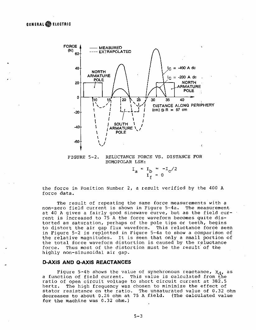
G E N E R A L ® ELECTRIC

FIGURE 5-2. RELUCTANCE FORCE VS. DISTANCE FOR HOMOPOLAR LSM:

the force in Position Number 2, a result verified by the 400 A force data.

The result of repeating the same force measurements with a non-zero field current is shown in Figure 5-4a. The measurement at 40 A gives a fairly good sinewave curve, but as the field cur­rent is increased to 75 A the force waveform becomes quite dis­torted as saturation, perhaps of the pole tips or teeth, begins to distort the air gap flux waveform. This reluctance force seen in Figure 5-2 is replotted in Figure 5-4a to show a comparison of the relative magnitudes. It is seen that only a small portion of the total force waveform distortion is caused by the reluctance force. Thus most of the distortion must be the result of the highly non-sinusoidal air gap.

D - A X IS A N D Q - A X I S R E A C T A N C E S

Figure 5-4b shows the value of synchronous reactance, x^, as a function of field current. This value is calculated from the ratio of open circuit voltage to short circuit current at 382.5 hertz. The high frequency was chosen to minimize the effect of stator resistance on the ratio. The unsaturated value of 0.32 ohm decreases to about 0.26 ohm at 75 A field. (The calculated value for the machine was 0.32 ohm.)

5 - 3

G E N E R A L ® ELECTRIC

i

I ARMATURE STACK

FIGURE 5-3. TWO POSITIONS OF SALIENCIES RELATIVE TO ARMATURE mmf DURING RELUCTANCE FORCE MEA­SUREMENTS. FORCE AT POSITION NUMBER 1 = 3 / 2 FORCE AT POSI­TION NUMBER 2.

The direct axis transient reactance was measured by recording the waveforms of one phase voltage and two phase currents during a step change from open circuit to short circuit on the stator with constant field current. One of the resulting waveforms is shown in Figure 5-5. The excitation frequency is 382 hertz. The enve­lopes of the waveforms have been traced to make them visible. The transient seen in the figure decays very quickly, in about 10 msec, in contrast to the behavior of small air gap machines where the decay may take several seconds. The time constant governing this decay is nearly equal to the ratio of field self-inductance to field resistance. Since the field flux crossing the air gap of a machine is inversely proportional to the length of the gap, the field inductance due to air gap flux in the LSM is several hundred times less than that of a round rotor synchronous machine. Because the field resistance is not a function of air gap, the subtransient time constant of the large air gap machine should be much smaller than that of the small air gap machine.

The value of the d-axis subtransient reactance is given by

i ssd Iini t

(5-1)

5-4

G E N E R A L I ELECTRIC

FIGURE 5-4a. FORCE VS. DISTANCE FOR HOMOPOLAR LSM;21 = 21. = I = 200 A dc.a d c

FIGURE 5-4b. LSM LAMINATED TRACK SYNCHRONOUS REACTANCE Xd VS. FIELD CURRENT - 382.5 Hertz, 1530 rpm.

5 - 5

GENERAL® ELECTRIC

0.05 S E CFIGURE 5-5. HOMOPOLAR LSM WAVEFORMS FOR AN OPEN CIRCUIT.

TO SHORT CIRCUIT STEP. FREQUENCY IS 382 HERTZ. FIELD CURRENT IS 75 AMPERES.

where X^ is the direct axis reactance, I3S is the steady state phase current, and Iinit is the initial value of the phase cur­rent. By this formula

X^ = 0.90 Xd « 0.27 Si 394 hertz (5-2')

where the saturated value of X^ has been used. This result is highly approximate due to the fast decay of the transient current.

Since the transient time constant was so short, no subtran­sient effects were visible. They should be slight since there are no amortisseur windings.

Two types of measurements were made to obtain a value of quadrature axis reactance. The first was a method based on reluc­tance torque given by Klingshirn^ which says

^1978 IEEE PES Winter Power Meeting.

5-6

GENERAL© ELECTRIC

where

8 TLd - Lq = 3 P I2 sin 2 6 m

(5-3)

L, = d-axis inductance dL = q-axis inductanceq MTq = developed torque in nt-m

P = number of poles (here saliencies)

I = dc current applied to armature m5 = torque angle in electrical degrees

The torque and current values of Figure 5-2 gives

8 x 66 x 0.67L, - L = d q 3 x 3 x 400 x sin(2 x 45 )(5-4)

The value of X.-X is then 0.606 @ 394 hertz. Since the unsat­urated value of Xj is 0.45 @ 394 hertz.

X a - 0.266 ft £ 394 hertz (5-5)

This negative value is clearly impossible. Further reflec­tion has led to the conclusion that the difference in inductances measured by this method on an inductor machine is (max)-Ld(min) where L^/max% is the d-axis inductance in the center of the inter- polar space and is the d-axis inductance at the center ofthe pole piece. It appears that the q-axis reactance is not re­lated to a static (dc excitation) force measurement in art induc­tor machine, a result caused by having saliencies only at every second direct-axis armature circuit.

The second method used to measure X was a slip test. For this measurement the machine was excited^by a three-phase 60 hertz sinewave voltage source and driven at slightly less than synchro­nous speed. The field was open circuited. Figure 5-6 shows the. waveforms of the b-phase voltage and current and the field voltage. The q-axis reactance is given by

XqV,X, min xd V.b max

I,b m mI,b max

(5-6)

= 0.34 x 0.92 x 0.91 = 0.284 ft @ 394 hertz

The reactance X^ has the unsaturated value. This value of Xg is quite reasonable.

5-7

G E N E R A L ® ELECTRIC

li

*b MIN

J _ _____

■b MAX

y ^ ___

PHASEB

CURRENT

vb MAXw PHASEvb MIN B, VOLTAGE

tVf MAX tvf MIN FIELDVOLTAGE

0.5 SECFIGURE 5-6. ENVELOPES OF PHASE VOLTAGE AND CURRENT WAVEFORMS

DURING SLIP TEST:V, I,„ _ v b min „ b min

q d I. V,^ b max b max

The values of and Xq are close to each other because leak­age flux (-50% of X^) is nearly equal for both reactances and be­cause the ratio of d-axis to q-axis mutual flux is less than 2:1. (The ratio can even be less than 1:1 for large per unit pole arcs.) This relatively small ratio results because d-axis flux has to cross one large air gap in addition to one small air gap, while the q-axis flux crosses two large (interpolar) air gaps. (Recall that there are saliencies only at every other electrical pole.)

C O M M U T A T I N G R E A C T A N C E M E A S U R E M E N T

According to the Linear Synchronous Motor Test Plan (June 24, 1977), the commutating reactance of the LSM is given by

Lk = 2 t \ / ^ 2 c ) (5-7)

5-8

G E N E R A L ® ELECTRIC

where t2 is the zero to peak rise time of phase currents and c' is the equivalent capacitance of the inverter commutating capaci­tors. Using the rise time of Figure 5-7d (rated thrust) the com­mutating inductance is

I

2 x (220 x 10 6) 11 2 x 90 x 10-6

109 yH

(c = 3/2 c , where c is the commutating capacitor), X,

X^ = 0.27 ft @ 394 hertz

this value Corresponds well to the calculated value of

(5-8)

is then

(5-9)

Xk = 0.5(X^ + Xg) (5-10)

also given in the LSM Test Plan since

x" b x' = 0.27 ft and x" « X = 0.27 ft (5-11)d d q qfor the 112 kw homopolar test machine.

F L U X M E A S U R E M E N T

The modulated dc characteristic of the flux of this machine makes obtaining of flux data difficult, at least in comparison with a conventional ac flux machine. A combination of measurement tech­niques, including Hall-effect Gaussmeter and flux coil measurements, were used.

D C F L U X D I S T R I B U T I O N

The machine was instrumented with coils wrapped around various parts and the coil terminals taken to a low-drift .integrator cali­brated in flux linkages or lines. The field coil was excited with dc ramped up from zero to 75 A in one or two seconds, and the link­ages read from the integrator output. Figure 5-8 shows the coil locations and the values of flux associated with each in the test.It should be noted that a substantial amount of leakage is unac­counted for, as the yoke flux t)>„ in the stator yoke structure ex­ceeds the sum of the stator leakage <i>v, , the gap leakage <f> and the rotor flux ^rt. This amounts to y •

<J> - ( ( J , + 4 > g + 0 r t ) = [ 6.06 - (1.65 + .37 + 2.34) x 106 ] ( 5-12)

or 1.7 x 10^ linkages that are not found by the test coils. The flux. <b is the leakage across the track between sides of the ma­chine,^5

5 - 9

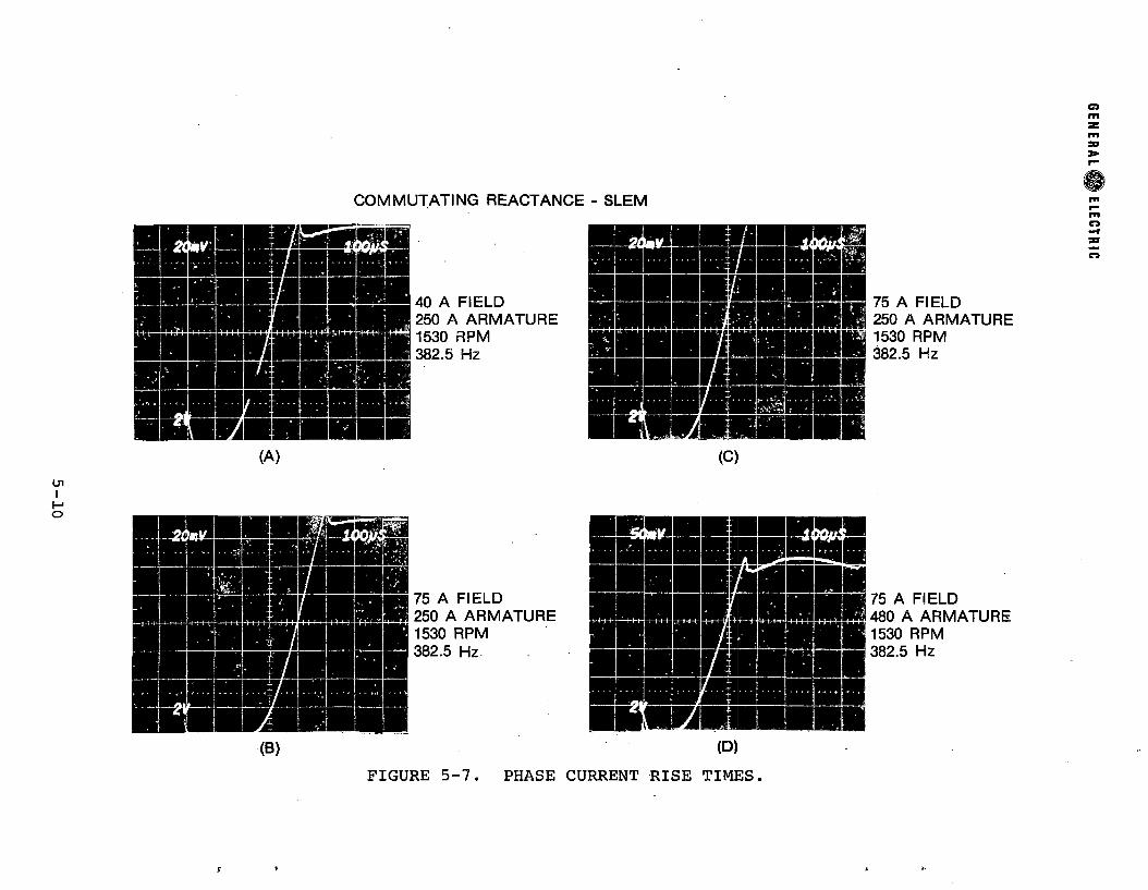
-1

0

C O M M U T A T I N G R E A C T A N C E - S L E M

Ul(A) (C)

•(B)

75 A FIELD 480 A A R M A T U R E 1530 R P M 382.5 Hz

FIGURE 5-7. PHASE CURRENT RISE TIMES.

f

GENERAL® ELECTRIC

FIGURE 5-8.

<f>

which amounts to

7 5 A F I E L D

< j> y = 6 . 0 6 X 1 0 6 L I N E S

<j>a = 5 . 3 6 X 1 0 ®

<f>y \ = 1 . 6 5 X 1 0 ®

i f ) g = .374 X 1 0 ®

< p n = 2.88 X 1 0 ®

< f > r c = 2.34 X 1 0 ®

<f) p = . 4 2 7 X 1 0 ®

( 3 S A L I E N C I E S O V E R

A R M A T U R E )

pi

LSM LAMINATED TRACK SEARCH COIL LOCATIONS FOR FLUX MEASUREMENT, DEFINITION OF FLUX COMPONENTS.

= <f> . - = [2.88 - 2.34] x 106rt rc l J (5-13)

= 0.54 x 10 lines

5= 0.036 x 10 lines per saliency.

These measurements also give an idea of the interpolar leak­age flux. As with three saliencies over the stator, the flux in each saliency is

= 0.427 x 10^ lines, P

5-11

GENERAL® ELECTRIC

while the total rotor flux is

<J>rt = 2.34 x 106 (5-14)

This leaves an interpolar leakage of

- * = 2.34 x 106 _ o 4 2 7 x 1 Q63 p 3

or 0.353 x 10^ lines per pole pair

(45% of airgap flux) which is flux crossing the air gap between saliencies, .making a negative contribution to the air gap flux variation.

(5-15)

These measurements also provide information on flux densities in the various parts of the machine. The density in the stator yoke is

Bg

6.06 x 1 0 lines n n n kl n or. L = t— co ‘ — nr- = 119 ---= 1.85 tesla.1.59 in. x 32 in. in.

Pole waist flux density is

427 x 10 lines . , 0 kl , n= 118 --- ~ = 1.82 tesla^p 1.71 in. x 2.125 in in.

while the pole surface is at

(5-16)

(5-17)

B, 427 x 10° lines „ kl , . „ . .= 72.0 — — ^ = 1.12 teslain.ps 2.79 in. x 2.125 in

and the stator teeth are at

„ _ .520 in. + .431 in. .. t o nr _B. = ------ ------------- x 1.12 tesla = 2.46 teslat .431 in.

(5-18)

(5-19)

when under a saliency, assuming no fringing. From these values, it is clear that the stator yoke, stator teeth, and pole waists are all saturated at 75 A field current.

INITIAL AIR GAP FLUX TESTS

Initial flux density measurements were made with a Hall-effect Gaussmeter. A probe was secured in the air gap over a stator tooth, field was applied to the machine, and'the wheel, or track, moved slowly by hand. The results of this test, for field currents of 30 and 75 A are shown in Figure 5-9. The peaks of flux correspond to the passage of track saliencies. For each of these cases a Fourier analysis was performed from the photos, and the dc average

5-12

GENERAL® ELECTRIC

----------5 SECONDS

30 A FIELD

IGAUSS

FIGURE 5-9. LSM LAMINATED TRACK QUASI-STATIC FLUX MEASUREMENTS (HALL GAUSSMETER).

and fundamental components were found. For the 30 A case, tfye dc average was 1.99 kG, and the fundamental was 1.38 kG. At 75 A field,, the dc average was 4.04 kG, and the fundamental was 2.68 kG. These values of fundamental agree fairly closely with the densities required to produce the open circuit voltages observed in earlier tests. Attempts to measure flux densities with the Hall Gaussmeter at operating speeds were unsuccessful due to the poor frequency response of the instrument.

The circuitry attached to the flux coils in the air gap con­sists of an ac-coupled integrator and a true-rms converter. For preliminary tests, a coil near the longitudinal center of the stator

5-13

GENERALI ELECTRIC

30 A FIELD

— -0 2400 GAUSS

____________ ± _(7.6 V l-n rms)

FIGURE 5-10. LSM LAMINATED TRACK FLUX MEASUREMENTS, FLUXCOIL NEAR CENTER OF STATOR - 240 rpm (17.4 m/sec).

was selected, and its circuit tapped to the oscilloscope before the rms conversion. Figure 5-10 shows the flux waveforms obtained at field currents of 30 and 75 A. Scaling these output voltages with circuit parameters and coil dimensions results in a conver­sion factor of about 0.16 tesla per volt. The machine was operated

5-14

G E N E R A L ® ELECTRIC

at 240 rpm (17.4 meters per second) for this test, and the rms terminal voltages were recorded as shown in the figure. The re­sults of this test, which indicate only the ac component, of flux, are in agreement with the Hall Gaussmeter measurements within the limits of accuracy of the two measurement devices.

In Figure 5-11 the results of a static test of flux density over a stator tooth are presented. At various field currents from zero to 100 A the track was moved over the Hall probe on the stator to find maximum and minimum flux densities. These values, as well as the difference between maximum and minimum, are presented. The difference, labeled AB , is closely related to the opencircuit voltage generated by tne^machine, and a comparison with Figure 5-2, for example, will show this. The AB actually decreases as the machine shows saturation in the vicinity of 100 A field current, just as the voltage decreases in this region.

FIGURE 5-11. SLEM STATIC TEST OF AIR GAP FLUX - HALL PROBE CENTERED OVER STATOR TOOTH.

Air Gap Fiyx at Operating SpeedsFigure 5-12 shows the peak ac component of flux density as

obtained from the stator flux coils through the data acquisition system. The three test frequencies were 60, 150 and 382.5 hertz, and there were no significant differences in the flux distribution with frequency. The shape of the distribution shows only a little variation of flux density from front to rear of the machine, and the magnitude is the same for all three cases. There is no end effect dependent on speed or frequency in the ac flux as seen from the stator side of the air gap.

5-15

GENERAL ELECTRIC

FIGURE 5-12. LSM LAMINATED TRACK PEAK AC FLUX DENSITY VS. SLOT POSITION - 60, 150, 382.5 Hertz.

Track Pole FluxA coil of five turns was wrapped around the body of one track

pole saliency and taken to slip rings, then to an oscilloscope or the DPO to be recorded. Figure 5-13 shows the voltage signals re­corded for several conditions. The first run, at 60 hertz with 15 A field, shows a ripple due to the action of the field rectifier The ripple frequency is 360 hertz, corresponding to the. six-times ripple frequency in the rectifier output. As the field current is increased, this ripple disappears, as shown in the 60 hertz,75 A case. The third case is one at rated speed and load and shows spikes due to current switching in the armature windings, these spikes appearing at six times the fundamental frequency, including both positive and negative going ones.

A second trace at the top of the third photo is the signal from the Number 2 Position sensor, which occurs when the track pole at the leading end of the machine is in the position indicated in Figure 5-14. This also corresponds to the greatest rate of change of flux (highest voltage) in the entrance period. The flux in the track pole begins to rise when the pole previous to it is entering over the stator, according to this test. The maximum decreasing flux occurs about 3.2 pole-pair pitches later, or approximately one inch after the theoretical end of the stator. Buildup and de­cay of flux appear to be symmetrical, and little or no end-to-end variation would be expected.

5-16

GENERAL m ELECTRIC

60 H E R T Z

15 A FIELD

0.5 V/DIV.

10 MSEC/DIV.

60 H E R T Z

75 A FIELD

1.0 V/DIV.

10 MSEC/DIV.

382.5 H E R T Z

75 A FIELD

480 A A R M A T U R E

R A T E D L O A D

5V/DIV.

2 MSEC/DIV.

FIGURE 5-13. LSM LAMINATED TRACK POLE COIL VOLTAGE.

5-17

GENERAL ELECTRIC

FIGURE 5-14. LSM LAMINATED TRACK - POSITION OF TRACK POLEOVER STATOR AT INTERRUPTION OF POSITION SENSOR NUMBER 2.

IN T E G R A T E D T R A C K C O I L S IG N A L S

The digital processing oscilloscope was used to record and process the voltage signal from the track pole coil under various operating conditions. Figure 5-15 shows the voltage obtained at 60 hertz speed with 40 A field applied. The DPO was used to di­vide this signal by the number of turns in the coil and integrate the result point-by-point with the1 result shown in Flcjure 5-16. The flux of 3.5 x 10 webers corresponds to a density of 1.49 tesla, and the pole waist is well below- saturation.

5-18

GENERAL H ELECTRIC

FIGURE 5-15. TRACK POLE COIL VOLTAGE VS. TIME - 60 Hertz, 240 rpm, 40 Ampere Field.

IE-3 'JS

FIGURE 5-16. TRACK POLE FLUX VS. TIME -60 Hertz, 240 rpm, 40 Ampere Field.

5-19

GENERAL ELECTRIC

A rather interesting time and position variation of flux in the pole appears in this unsaturated case. There is a general slope upward from front to rear of the machine, amounting to about0.2 x 10 webers, and there are two dips in this slope. The dips correspond to the entrance of the succeeding saliencies over the stator and the departure of the preceding ones. This slope and the dips indicate that the flux in the air gap and in the stator iron structure does not re-distribute instantaneously with the en­trance and exit of saliencies, and that, in fact, the solid iron stator yoke influences the re-distribution of flux in a minor way. The solid iron structure delays the re-distribution of flux as a new saliency enters and causes a slight pileup of flux at the rear of the machine. The dips occur as the flux in each saliency is shared with the new entering one.

Figure 5-17 shows the flux in the track pole at 60 hertz speed with 75 A field applied. The effective length and approximate position of the stator core are also shown as they relate to the time scale. The peak flux of nearly 5 x 10-3 weber corresponds to a density of about 2.1 tesla. Figures 5-18 and 5-19 show the flux at 150 hertz speed and 382.5 hertz speed, respectively, and, except for time scale, these are identical to Figure 5-17. No effect of speed on flux buildup or maximum flux can be observed in these figures, and these results agree with those of Figure 5 -12 in showing the absence of any appreciable end effect in the machine.

FIGURE 5-17. TRACK POLE FLUX VS. TIME (POSITION) -60 Hertz, 240 rpm, 75 Ampere Field.

5-20

G E N E R A L ® ELECTRIC

I E - 3 U S

FIGURE 5-18. TRACK POLE FLUX VS. TIME (POSITION) - 150 Hertz, 600 rpm, 75 Ampere Field.

I E - 3 U S

FIGURE 5-19. TRACK POLE FLUX VS. TIME (POSITION) -382.5 Hertz, 1530 rpm, 75 Ampere Field.

5-21

G E N E R A L ® ELECTRIC

S e c t io n 6

M O D I F I C A T I O N S A N D C O R R E C T IO N S T O T H E H O M O P O L A RI S M D E S IG N P R O G R A M

The Homopolar Linear Synchronous Machine presently under test was designed with large margins of safety since the behavior of this type of machine was not well understood. First, a four-pole machine was designed which was to deliver rated thrust with 120 kW of input power. Then a fifth pole was added to the stator and taps installed so that, if necessary, the thrust could be increased by 25%. It resulted that the designer’s prescience in over-de- signing the. LSM ?n this way nearly compensated for the defects of the design program he was using. While the design program said the five-pole test machine should have an input power of 150 kW, the actual machine had only 95 kW of input power. (Input power is used as a performance measure since the program does not calcu­late losses.) By increasing the armature current above the design value, it was possible to achieve the 112 kW output power specified in the proposal.

It was thus clear that the design program had to be improved before it could be trusted to give the correct dimensipns for a full-sized machine of a given rating. The program has now been modified, and agreement with the test machine data is much better. This section will describe the corrections made to the design pro­gram to achieve this improvement.

FORM FACTORS K AND K sam yThe design program begins by reading the values of the form

factors which establish the relationship between ac, dc, and peak flux density. Once these values are established, the program uses vector analysis and flux density calculations to determine the minimum required dimensions for the machine. These calculations are very similar to those performed in much more successful machine design programs. Therefore, unless this portion of the program contained a significant error, it was likely the greatest problem was with the form factor determination. When a careful study of the vector and flux density calculations revealed no major errors, a study of the form factors was begun.

The factors studied are designated and Ku. The factor K is the ratio of peak air gap flux density to average air gap flux density. The factor Ku is equal to the total dc flux per pole divided by the ac fundamental flux per pole. Figure 6-1 shows the definition of Km and Ku in terms of quantities measured from an air gap flux waveform. The values of and Ku depend on the peak air gap flux density, the minimum air gap flux density, and fringing. The corrections made to the design program modify the value of the minimum air gap flux density to reflect the small (compared to conventional round machines) minimum-to-maximum air gap ratio and the effect of inter-armature leakage flux.

6-1

G E N E R A L S ELECTRIC

B max ^ T O T A L D C F L UX 7rBav

Bav u “ FUND. A C F L UX ” B^~"

AIR G A P F L UX DENSITY

A R M A T U R E IRONX X X X X X X X X X X x X

7-777777/ '/ /V ' ' ' 'A

SALIENCIES y ? / / / n ' /v // ///' ' ' ' '

FIGURE 6-1. DESCRIPTION OF FORM FACTORS K AND K .m uDEPENDENCE OF K m AND K u ON AIR GAP RATIO

The values of Km and are obtained from curves generated by flux plotting and assumea minimum-to-maximum gap ratio pf 1/10 For small air gap machines these curves are quite satisfactory, but as the air gap ratio decreases, Km and K begin to change rap - idly. To find their dependence on air gap, the geometry of Fig­ure 6-2 is used.

To simplify the calculations, the actual air gap flux distri­bution is replaced by a rectangular wave approximation. The aver­age flux density is then

B a V " Bmax<“'/2) + Bm l n ( l - o V 2 ) (6-1)

6-2

GENERAL® ELECTRIC

AIR GAP FLUX DENSITY

fku w tr

Bmax

B min ""

r xi i\

A P P R O X I M A T E D 17—/ B(x) A i\

f i i >

! i \ / \ A C T U A L /\ / B(x> /

f | ' >1 1 !1 11 1

_i i _ .

V / \ ✓

1 1 1 1

wtr

0 TSTATOR

2T DISTANCEALONG TRACK

ROTORFIGURE 6-2. GEOMETRY FOR CALCULATION OF K AND K

FOR VARYING GAP RATIO.

where a 1

a

fkuBmaxBmin

per unit pole arcpole arc 'fringing' coefficientmaximum flux densityminimum flux density

The assumption that the flux density varies as the inverse of the air gap gives

BaV = Bmax[(a'/2) + (gl/g2)(1-a'/2)1 : (6_2>

6-3

GENERAL® ELECTRIC

where g^ and g2 are the minimum and maximum air gaps, respectively.The value of is thenm t

BKm = B

maxaV

2/a'[1 + (g1/g 2) (2 -a ' ) /a ' ]

Since the Km curves assume g^/g2 = 0.1

(6-3)

= 1 + 0.1 (2-g1 )/a1Ro ckm 1 + (93 /9 2 ) (2-o?)/a' (6-4)

where K° is the value of K from the flux plotting curves, m mThe fringing coefficient f. =a'/a is found by solving Eq.

6-3 for f^m yielding_ 2-2(gi/g2)Km

km aKm-[l-(g1/g2)] 1

and evaluating Eq. (4-5) at (g^/g2) = 0.1 to give

2 - 0.2 K°f. = -------- -km 0.9 a K° m

(6-6)

A corrected value of Km is then calculated as k . The processis iterative since the value of the interpolar gap, g2, depends on K . A summary of the procedure will be given later in this report.

From Figure 6-1 the value of Ku isi t B

K = uaV T T B max BaV T T B.

Bal. Bal Bmax Bmax 1

K (6-7)al m

Thus combining Eq. will be sufficient

6-4to

with the effect of gap ratio on derive the gap ratio correction

Using the geometry of Figure 6-2, the fundamental fourier coefficient of the rectangular-wave flux density approximation is:

6-4

G E N E R A L ® ELECTRIC

Bal 2T

a'T/ 2

/ Bmax Cos p dx + | J

a ' T/2

7TXBmin Cos dx

2 „ . a' tt- B sin —7]- insx Z2 . a ' tt— B ■ „ s m —75— 7f min Z (6-8)

2 Bmax ,, , , . a'Tr--- (l-gj/92) sin ~J~where

T = electrical pole pitch

a ! = fR u a

f^u = Ku fringing coef.

a = per unit pole arc

The value of Ku is then

K _ jr_ u Km

772 (l-g^/^) sin (a' tt/2 ) (6-9)

The ratio of Ku to K^, the value given by the flux plotting curves, is

K

Kuo - cku 'u

£ 1 1 ^ 4 ) - , (6-1 0 )m 1 gl/g2/ ck m [1 gl/g2 )]

The procedure to calculate the correct value for K is again iter­ative since the interpolar gap is a function of K .

I N T E R A R M A T U R E F L U X C O R R E C T IO N

The path for interarmature flux is. shown in Figure 6-3a.This flux increases the flux density in the interpolar region and changes the values of and Ku in much the same way as decreasing the interpolar gap does. Therefore, a relatively simple way to correct for the effect of interarmature flux is to decrease the effective interpolar gap.

The first step in determining this new gap is to calculate a permeance for the interpolar gap. The formula given by Professor Enrico Levi of Polytechnic Institute of New York

PIA = (VQ / n ) £n U + wa/wf)

6 - 5

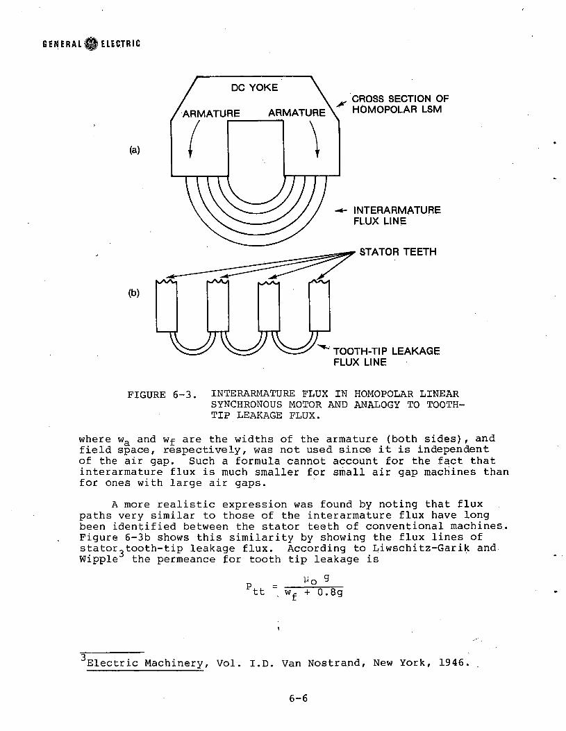
G E N E R A L ® ELECTRIC

FIGURE 6-3. INTERARMATURE FLUX IN HOMOPOLAR LINEAR SYNCHRONOUS MOTOR AND ANALOGY TO TOOTH- TIP LEAKAGE FLUX.

where wa and Wf are the widths of the armature (both sides), and field space, respectively, was not used since it is independent of the air gap. Such a formula cannot account for the fact that interarmature flux is much smaller for small air gap machines than for ones with large air gaps.

A more realistic expression was found by noting that flux paths very similar to those of the interarmature flux have long been identified between the stator teeth of conventional machines. Figure 6-3b shows this similarity by showing the flux lines of statortooth-tip leakage flux. According to Liwschitz-Garik and WippleJ the permeance for tooth tip leakage is

P = 9tt w + 0 .8g

1

3 Electric Machine Vol. I.D. Van Nostrand, New York, 1946.

6-6

G E N E R A L ® ELECTRIC

where g is the air gap. This formula is the result of a curve fit to data obtained by plotting the flux lines of a geometry like that of Figure 6-3a, further strengthening the argument that Eq.6 - 1 1 is a good representation of interarmature flux permeance.Thus the permeance for interarmature flux wili be taken as

PIA^o 92

wf + 0 . 8 g2(6-11)

where g2 is the interpolar gap. The flux density due to inter­armature flux is then

BIAPIA x mmfa

wa/2 (6-12)

where mmf is the armature mmf. The interpolar flux density due to flux wBich enters the iron in the interpolar region is

B . m mU0 nunfa

(6-13)

which gives a ratio of BT7V to B„. as 3 IA min

b ia 2 92 (6-14)B . min wa (wf + 0.8 g2)

The effect of interarmature flux can now be incorporated into Bm ^n to form

BIAB = B j 1 + _ m m m m 1 B_.ii mmf Ho a (6-15)

m m ,

where g2 is a corrected interpolar air gap and is given by

-19o = 9- 1 +

2 g.

wa (Wf + 0.8g2)

>2 "g (w£ + 0 .8g2)9o wswa (Wf + 0.8g2) + 2 g2

(6-16)

The revised design program replaces the calculated interpolar gap, g2, by the value g2 to account for. the effect of interarmatureflux.

6 - 7

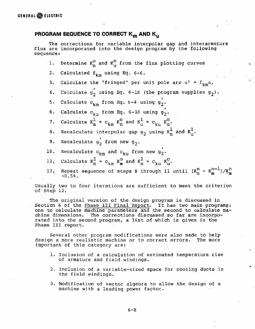
GENERAL ELECTRIC

PROGRAM SEQUENCE TO CORRECT K m AND K yThe corrections for variable interpolar gap and interarmature

flux are incorporated into the design program by the following sequence:

1.2.3.4.

5.

6.7.

8. 9.10.11.12.

Determine K° and K° from the flux plotting curves m u r 3

Calculated f^ using Eq. 6-6 .

Calculate the ’fringed' per unit pole are a ’ = f^a.I

Calculate g2 using Eq. 6-16 (the program supplies g2 >I

Calculate c^ from Eq. 6-4 using g2 *I

Calculate from Eq. 6-10 using g2 *

Calculate kJ = c, K° and K?; = c. K°.m km m u ku uRecalculate interpolar gap g2 using and Ku -

IRecalculate g2 from new g2 »

IRecalculate c,_and c,,„ from new g2 *'km 'kuCalculate = c. K° and = c. „ K°.m km m m ku uRepeat sequence of steps 8 through 11 until (K^ - K^_<0.5%.

Usually two to four iterations are sufficient to meet the criterion of’Step 1 2 .

The original version of the design program is discussed in Section 6 of the Phase III Final Report. It has two main programs: one to calculate machine parameters and the second to calculate ma­chine dimensions. The corrections discussed so far are ingorpo- rated into the second program, a list of which is given in the Phase III report.

Several other program modifications were also made to help design a more realistic machine or to correct errors. The more important of this category are:

1. Inclusion of a calculation of estimated temperature rise o,f armature and field windings.

2. Inclusion of a variable-sized space for cooling ducts in the field windings.

3. Modification of vector algebra to allow the design of a machine with a leading power factor.

6 - a

GENERAL ELECTRIC

4. Inclusion .of field yoke ampere-turns into design procedure.

5. Modification of tooth-tip and end-turn armature leakage reactar:e calculations.

Modification Number 1 showed a serious heating problem in the field windings contained in the interpolar space.

VERIFICATION OF CORRECTIONS FOR 112 k W TEST LSM

As a verification of the modified design program a type of backward design was performed for the 112 kW homopolar linear syn­chronous machine presently being tested. Since the total length of the machine is fixed by the speed, frequency, and number of poles, armature width is the most important single dimension which specifies a machine's flux distribution and power. Accordingly, the rated voltage in the design program's input data was varied until the designed machine had the same armature width,as the test LSM. Table 6-1 compares the main parameters and dimensions of the machine so designed to the test machine values. The first column of the table lists these values as given by the unmodified design program (in the run which finalized the test machine's dimensions).

The flux density levels needed to calculate the test values of K and Ku are taken from Section 5 of this report. These give the 75 A field current values of

Km = - l -*3 (6-17>and

Ku = H r k r 1 = 4-74 {6“18)

The correlation to the modified design program values of Km = 1.75 and K = 4.83 is very good. In addition the field current of the design program is 90 A while that of the test machine (for this data) is 75 A. A higher field current would lower K and raise Ku because of saturation effects, further improving tihe agreement.

The values taken from the original design program of K = 2.03 and I< = 2.82 show K was reasonably close but the Ku was almost 60% too low. The ef¥ect of this error in K was to underestimate severely the total flux which had to cross the air gap to make a given rating. Thus when the originally calculated value of total air gap flux crosses the air gap of the test machine, the power delivered is only about 60% of the designed value.

This result is seen in the power calculations for the design programs and the test machine. While the December 1976 design said the machine would have an input power of 3 x 370 x 140 = 156 kW, the test machine had only 3 x 370 x 120 x 0.7 = 93 kVJ. The

6 - 9

GENERAL ELECTRIC

TABLE 6-1. COMPARISON BETWEEN TEST DATA AND ORIGINAL AND REVISED VERSIONS OF DESIGN PROGRAM FOR 112 kW HOMOPOLAR LSM

Dec. '76 Design Program (final de­sign run

April '78DesignProgram

TestData

Speed (mphj 250.000 250.000 250.000Frequency (Hz) 394.300 394.300 394.300Poles 5.000 5.000 5.000P.U. Pole Arc 0.500 0.500 0.500Phase Current (A) 370.000 370.000 370.000Voltage (L-N) 140.000 87.000 120.000Power Factor 1.000 1.000 0.700Phase Resistance (ft@40°C) 0.0134 0.0134 0.011Arm. Leak. Reac. (ft) 0.165 0.143 -d-axis Reac. (ft) 0.312 0.308 0.30+.01d-axis Reac. (ft) 0.284 0.279 0.27+.01d-axis Trans. Reac. (ft) 0.239 0.265 0.27+.02Commutating Reac. (ft) 0.261 0.272 0.27+.01

(ratio dc to ac flux) IT; (ratio peak to aug.

flux density)

2.82 4.83 4.74

2.03 1.75 1.83Field Current (A) 75.30 90.80 85.00Field resistance (ft@75°C) - 0.64 -Stator width (cm) 25.00 25.00 25.00Stator length (cm) 70.90 70.90 70.90 ,Stator height (cm) 9.08 12.47 -Stator weight (kg) 170.00 212.00 -Pole piece height (cm) 7.48 8.53 7.62Pole piece weight (kg) 10.40 11.80 -

modified design program now says the test machine's input power would be 3 x 370 x 87 = 97 kW, a marked improvement.

Taken together, the results of this section indicate that the original design program did a poor job of determining the di­mensions of the large air gap homopolar linear synchronous machines being studied; but also that the program as now modified shpuld accurately determine the required size of the full-scale linear synchronous motors which appear in the Phase III SLEM final report.

6-10

GENERAL w&) ELECTRIC

Section 7e x p e r i m e n t a l d a t a

In this section, the method of data collection and reduction is explained, and the computer program(s) used for data reduction presented. A catalog of Appendix I is also included.

DATA ACQUISITIONThe data presented here for the LSM was obtained using the

data acquisition system described in Section 1 of the Phase II report, with appropriate changes of channel assignments to func­tion with the synchronous machine. Table 7-1 contains a listing of the data channel assignments for this motor. Most of these are self-explanatory, but a few comments are in order. The force sensors A through J are ordered as shown in Figure 4-1'of Sec­tion 4. The airgap flux coils are centered over the odd-numbered stator slots, Numbers 1 - 3 5 (18 coils), while the yoke coils are wound around the laminated stack from the bottom of the associated slot to the bottom of the laminations. The butt coils cover the ends of the laminated stacks to measure axial flux out the ends.

Phase voltages and currents are measured as true rms values, while phase watts are averaged over time. The inverter firing angle signal is a dc voltage in the inverter control related to the angle-of-lead of firing pulses ahead of motor back emf. Speed and torque signals are averages coming from the shaft torque transducer, while dc link volts and amperes are averaged values from a scope probe and a current transducer attached to the link between rectifier and inverter.

The vertical force sensors can go both positive and negative in force, so their data channels have been given a 5.00 volt off­set, upward force reducing the output voltage, downward increas­ing it. The lateral force sensors were preloaded against each other in pairs, as were the thrust or axial force sensors. This procedure increased the ability of the system to measure rela­tively small forces on the stator.

The airgap flux coils, all 18 of them, were 0.951 in. x 2.36 in. (2.42 x 5.99 cm) and were connected through RC integrators to produce a signal proportional to the ac flux cutting them.The yoke and butt coil outputs were treated similarly, but their areas differed. The yoke coils at Slots Numbers 6 and 30 were 4.938 x 2.313 in. (12.54 x 5.88 cm), at Slots Numbers 12 and 24 were 3.156 x 2.313 in. (8.02 x 5.88 cm), and the one at Slot Num­ber 18 was 2.563 x 2.313 in. (6.51 x 5.88 cm). The butt coils were 1.813 x 7.063 in. (4.60 x 17.94 cm). All of these coils were treated to give flux densities as output in the data reduction program but can be used to give total flux, with the dimensions above.

7-1

TABLE 7-1. LSM DATA CHANNEL ASSIGNMENTS

1 - 3 Phase Volts A,B,C respectively4 - 6 Phase A, A , B ,C respectively7 - 9 Phase Watts A,B,C respectively10 Firing Angle of Inverter11 Speed12 Torque13 dc Link Volts14 dc Link A15 - 18 Vertical Force Sensors A - D, respectively19 - 22 Lateral Force Sensors E - H, respectively23 - 24 Axial (Thrust) Force Sensors I, J respectively25 Not Used26 - 43 Airgap Flux Coils44 - 48 Not Used49 Yoke Flux Coil @ Slot #650 Yoke Flux Coil @ Slot #1251 Yoke Flux Coil @ Slot #1852 Yoke Flux Coil 0 Slot #2453 Yoke Flux Coil 0 Slot #3054 Butt Flux Coil - Lead - 752 Side55 Butt Flux Coil - Lead LSM Side56 Butt Flux Coil Trail - 752 Side57 Butt Flux Coil Trail - LSM Side58 Not Used59 Temperature - Endturn Near Slot #860 Temperature - Endturn Near Slot #1661 Temperature - Endturn Near Slot #2362 Temperature - In Slot, #863 Temperature - In Slot, 752 Side, #1664 Temperature - In Slot, 752 Side, #2365 Temperature - In Slot, LSM Side, #1666 Temperature - Care, LSM Side, Near Slot #867 Temperature - Dogbone68 Temperature - Yoke69 Temperature - Inboard Bearing70 Temperature - Outboard Bearing71 dc Motor Armature Volts72 dc Motor Armature A73 dc Motor Field A74 Not Used75 LSM Field Volts76 LSM Field A77 Not Used

7-2

G E N E R A L ® ELECTRi C

Temperature channels were noisy in operation, but the average of three readings proved fairly accurate during testing. The dc motor armature current channel was never made meaningful, but volt­age and field current were fairly accurate. LSM field voltage and current were obtained from the field rectifier output, averaged to get rid of rectifier ripple.

A sample data reduction program showing the conversion factors and logic used and a sample run from that program follow (Figure 7-1). These examples are from the analysis of the solid track machine, but differ only in minor detail from the laminated track ones. Varia­tions on this program were made to suit different speeds and motor­ing and generating conditions as necessary. These variations in­cluded changes to voltage and watts channel calibrations, friction and windage calculations, and sign changes on torques and watts, and have not been included here due to their simple nature.

10*)>RUN*»TSSLIB/RLINE,R=(NWARN)#DATA"IO"20 CHARACTER P0S*l(10)/lHA,IHB,IHC,1HD,1 HE,1HF,IHG,1HH,1 HI,IHJ/30 CHARACTER POBUTT*I(2)/lHI,1H0/40 REAL NMI,NM2,NM3,MAX1,MAX250 REAL MAX3,MAX4,MAX5,MAX6,MAX7 60 CHARACTER ST0RE+I8,ST0RI*30 70 CHARACTER DATE*8,TIME*5 80 DIMENSION ISTART(5),C(400),F2(10)90 DIMENSION V(3)100 DIMENSION F(I0)110 CHARACTER IBUF*72120 INTEGER RN0, DRPM, HZ, AMP1 30C140C IDENTIFICATI0N(DATE,TIME,RUN NUMBER,RPM, FREQUENCY,150C AND AMPS) IS READ FROM THE FIRST160C LINE OF FILE "DATA" AND PRINTED AT THE TOP OF THE REPORT.I70C THE FIRST 2 ITEMS ARE IN THE FORM XX/XX/XX AND XXiXX I80C AND THE REMAINING ARE INTEGERS. ALL ITEMS ARE SEPARATED I90C BY BLANKS.200C2 IOC220 READ (10,20) DATE,TIME,RN0,DRPM,HZ,AMP 230 PRINT 66240 66 FORMAT(1 X////////"DATE" ,T11,"TIME",TI 9,"RN#",T26,"RPM",250 & T35,"HERTZ »,T45,"AMPS"//) :260 PRINT 67,DATE,TIME,RN0,DRPM,HZ,AMP270 67 FORMAT(IX,A8,TI2,A5,TI9,I4,T27,I4,T35,I4,T45,I4,280 & //////)290 LSW=3 300 1=131 0C320C THE REMAINING DATA ITEMS ARE READ AND PLACED IN THE ARRAY 330C (C). POINTERS ARE SET UP TO THE BEGINNING OF THE THREE SETS'340C OF UATA(-1 SIGNALS THE END OF A DATA SET) -2 SIGNALS THE 350C END OF DATA(THE FIRST ITEM IN EACH SET IS THE STARTING 360C CHANNEL NUMBER,WHICH IS IGNORED).370C380 10 CALL RLINE(10,IENT,LSW, IBUF,$30,S50,S50)390 DECODE(IBUF,20)(C(I),1=1,I+(IENT-I))400 1=1+1410 20 FORMAT(V)420 GO TO 10430 30 N=l440 I START(N)=2450 DO 40 M=I,I460 IF(C(M).ME.—I)G0 TO 40470 IF(C(M+I).EQ.-2)G0 TO 60480 N=N+1490 ISTART(N)=M+2500 40 CONTINUE510 50 PRINT," ERROR RETURN"520 GO TO 310 530 60 PRINT 65540 65 FORMAT(IX."SENSOR#",T1 5." I ST READING",T30,"2ND READING",

FIGURE 7-1. SAMPLE RUN FROM A SAMPLE DATA REDUCTION PROGRAM.

7-3

550 & T45,"33D READING",T60,"AVERAGE")560C570C THE TH«6E SETS OF DATA ARE AVERAGED HH3 THE VALUES STORED 5800 AT THE END OF ARRAY (C). THESE VALUES ARE USED IN' THE 590C CALCULATIONS. THE 3 VOLTAGE READINGS AND THE 600C AVERAGE ARE PRINTED OUT.61 OC620 I l=ISTART(I)II2=1 START(2);13=ISTARTC3)!I4=n+I630 DO 62 1=1,ISTART(2)-4640 C( 14) = (C(I I)+C(I2)+Ct13)J/300.650 PRINT 64,I,CIII )/100.,C(I2I/1 00.,C(I 3)/100.,C<14)660 64 FORMAT ( IX, T3,12, T14, F7.4 , T2 9, F7.4, T44, F7.4 , T5 9, F7.4)670 11=11+U 12=12 + 1 ? 13=13+1114=14 + 1680 62 CONTINUE690C700C THE REMAINDER OF THE PROGRAM DEALS WITH MAKING CALCULATIONS 71OC (MULTIPLYING THE CONVERSION FACTOR BY THE VOLTAGE READING720C FROM THE TAPE) AND PRINTING THEM FOR THE FIRST 79 SENSOR 730C READINGS,74 OC750 IB=M+1i13=1 760 PRINT 23 770 STORE="VQLTS"780 PRINT II,STORE790 II FORMAT (11 LI NE" ,T20 , "SENSOR#" ,T40, "C FACTOR" ,T60, A.6 )800 DO 80 1 = 1 ,3 810 IF (I.EQ.1) VI=140.1 I 820 IF (I.EQ.2) V1=I 39.34 830 IF (I.EQ.3) V I = I 37.10 840 V2=V!*(C(IR))—1 850 V(I)=V2I 860 PRINT I 2,1,IS ,V1 ,V2870 12 FORMAT (12 , "-N" ,1'22,11 ,T39, FI 0.4 ,T58 , FI 0.4 )880 IS=IS+H IB=IB+I 890 80 CONTINUE 900 PRINT 24 910 STORE="AMPS"920 PRINT 11,STORE 930 V0LAMP=0.940 DO 90 1=1,3 950 IF (I.EQ.!) A1=94.97 960 IF (I.EQ.2) A1=96.71 970 IF (I.EQ.3) AI=94.44 980 A2=AI*(C{IF))990 V0LAMP=A2*V(I)+VOLAMP 1000 PRINT 12,I,IS,A1,A2 1010 IS=IS+IiIB=IR+I 1020 90 CONTINUE 1030 PRINT 25 1040 STO R E="K WATTS11 1050 PRINT II,STORE 1060 RK3=0.1070 DO 100 1=1,3 1080 IF (I.EQ.!) RKI=12.704 1090 IF (I.EQ.2) RK1 = 14.155 1100 IF (I.EQ.3) RKI=11.724 .MIO RK2=RK1*(C(ID)) •I 120 PRINT 12,1,IS,RKI ,R.K2

FIGURE 7-1. SAMPLE RUN FROM A SAMPLE ]

130 R K 3 = R K 2 + R K 3 140 I S = I S + I S l B = I B + l 150 100 C O N T IN U E 160 P R IN T I 2 2 . R K 3170 122 FORMAT( 1 X / T 3 9 , " T O T A L KW AT TS=” , T 5 b , F1 0 . 4 / )180 P R I N T 44190 44 F O R M A T ( IX , / / T 2 0 , 4,S E N S 0 R # " , T 4 0 , " C F A C T O R " )20 0 13 FORMAT ( I X , A I 8 , T 2 2 , I 2 , T 3 9 , F I 0 . 4 , T 5 8 , F I 0 . 4 )2 1 0 DA I = 3 0 . 9 322 0 DA2=L)A I*C CC I R ) 1 - 8 5 . 723 0 S T O H E = "D E L T A A N G LE "2 4 0 P R IN T 1 3 , S T O R E , I S , D A I , DA2 2 5 0 I B = I B + I S I S = I S + I 260 R S I = 2 0 0 .2 7 0 R S 2 = R S 1 * ( C ( I R ) )28 0 S T O R E = "R O T O R S P E E Q ( R P l ' ) "2 9 0 P R IN T 1 3 , STORE:, I S , R S I , R S 2 30 0 I B = I n + U I S = I S + 1

1310 NM1= 3 0 0 .320 N M 2 = N M I* ( C ( I B ) )

1330 S T D R E = "5 H A F T T O R Q U E (N M ) "340 P R IN T I 3 , S T O R E , I S , N M 1 , N M 2

1350 F W = . 0 0 0 2 0 6 3 3 * ( D R P M * * 2 . 0 )1360 S T D R E = "F S W T O R Q U E (N M ) = " ; P R IN T I 3 , STORE , I S , NM. I , FW 370 NM3=FW+NM2380 S T O R E = " E L E C T R O —MAG TORQUE (NM ) = " 5 P R IN T I 3 . S T 0 R E , I S , N M I , N ’-'3

1390 I B = I B + I » I S = I S + I 4 0 0 U C V I = 3 4 . 9

1410 D C V 2 = D C V l * ( C ( I 3 ) )4 2 0 . S T O R E = "D C L I N K V O L T S "

1430 P R I N T 1 3 , S T O R E , I S , D C V I , DCV2 4 4 0 I B = I B + I 5 I S = I S + |4 5 0 U C A 1 = 1 0 2 .64 6 0 D C A 2 = D C A I * ( C ( I B ) I4 7 0 S T O R E = "O C L I N K A M P S "4 8 0 P R I N T I 3 , S T O R E , I S , DCA I , DCA24 9 0 I B = I 8 + I » I S = I S + I5 0 0 C5 1 OC C A L C U L A T E AND P R IN T POWER OUTPUT V A L U E S .5 2 0 C53 0 R K W = N M 3 *D R P M * .0 0 0 1 0 4 7 7 540 H P = 3 K W / .7 4 6 5 5 0 T R = N M 3 / . 6 9 2 9 56 0 E F = ( R K W / R K 3 ) * 1 0 0 .5 7 0 P R I N T 455 8 0 STDR1 = " j( W = " S P R IN T 4 2 , S T 0 R 1 , R K W59 0 S T O R 1= « H P = " »PR I NT 4 2 . S T 0 R I , H P6 0 0 S T O R 1 = "T H R U S T (N E W T O N S ) = " J PR I NT 4 2 . S T 0 R I , T R6 1 0 ST O R I = " E F F ( N 0 T IN C F L D ) = " « P R I N T 4 2 , S T 0 R 1 , E F6 2 0 P O F A = 10 0 0 . 0 * R K 3 * 1 0 0 . O/VQLAM P63 0 S T O R l = “POWER F A C T O R ( % ) = " ; P R I N T 4 2 , S T O R I , P O F A6 4 0 S T O R I = » < V A = “ 1 P R I N T 4 2 , S T O R 1 , ( V O L A M P / 1 0 0 0 . 0 )6 5 0 ST O R I = » E F F X P F ( P U ) = » J P R IN T 4 2 , S T O R I , ( E F * P O F A / l 0 0 0 0 . 0 )6 6 0 C FREQ I S CAL FROM H E A D IN G RPM6 7 0 S T O R I = JI FR E Q U EN C Y ( H Z ) = " I P R IN T 4 2 , STOR I , ( . 2 5 *D RPM )6 8 0 P R IN T 26

1690 P R IN T 141700 14 FORMAT( I X , “P O S I T I O N " , T 2 0 , " S E N S O R # " ,T 4 0 , " C F A C T O R " , T 6 0 , " N E W T O N S " )

DATA REDUCTION PROGRAM (CONTINUED).

GENERAL® ELECTRIC

17 IO CI7 2 0 C THE 10 FORCE C A L C U L A T IO N S A R E ST O R E D I N ARR AY <F2) TO B E U S E D 1730C IN THE LAT ER C A L C U L A T IO N S ON TH E F O R C E S .I7 4 0 C1750 F ( I ) = 8 9 0 . I F ( 2 ) = F ( I ) I F ( 3 ) = F < 1 ) ( F ( 4 ) = F ( I )1760 F C 5 ) = 5 5 0 . ( F ( 6 ) = F ( 5 )1770 F < 7 ) = 5 5 8 . ( F ( 8 ) = F ( 7 )1780 F < 9 ) = 4 5 6 . 7 9 » F ( 1 0 ) = F ( 9 )I 7 9 0 C1800 DO 109 1 = 1 ,418 IO C A T T R A C T IO N PRODUCES A P O S I T I V E F ( 2 ) FOR 1 = 1 ,4 1820 F 2 ( I ) = F ( I ) * ( 5 . O O - C C I B J )1830 P R IN T I 5 , P 0 S ( I ) , I S , F ( I ) , F 2 ( I )1840 I B = I B + 1 ? I S = I S + I 1850 109 C O N T IN U E 1860C1870 DO 110 1 = 5 ,1 0 1880 F 2 ( I ) = F ( I ) * ( C ( I B ) )1890 P R IN T I 5 , POS C I ) , I S , F ( I ) , F 2 ( I )1900 15 FORMAT( 3 X , A 1 , T 2 2 , I 2 , T 3 8 , F I 0 . 4 , T 5 8 , F I 0 . 4 )1910 I B = I 8 + 1 ( I S = I S + 1 1920 110 C O N T IN U E 19 3 Q C

I 9 4 0 C A NUMBER OF C A L C U L A T IO N S ARE MADE U S IN G THE FORCE V A LU E S 1950C IN THE ARRAY ( F 2 ) AMD P R IN T E D OUT BY TH E ST A T E M E N T S FOLLOW ING. 1960C1970 R A D = .6 9 3 ; R L = . 7 6 2 ( W = . 15241 P = . 2 0 31980 C I = ( F 2 ( 1 0 ) - F 2 < 9 ) ) / ( F 2 ( l ) +F2 ( 2 ) + F2 ( 3 ) +F2 (4 ) )1990 B E T A = A T A N ( C I )2 0 0 0 R E S = ( F 2 ( I 0 ) - F 2 ( 9 ) ) / S I N ( B E T A )2010 C C 2 = ( ( ( F 2 ( 4 ) + F 2 C 3 ) - F 2 ( 2 ) - F 2 U ) ) * R L ) / 2 . 0 ) + ( F2 ( 9 ) - F 2 (1 0 ) ) * ( R A D + P ) 2 0 20 A L P H A = A R S I N I ( S I N ( B E T A ) * C C 2 ) / ( R A D * ( F 2 ( 9 ) - F 2 C ! 0 ) ) ) )2030 T H E T A = B E T A -A L P H A 2040 A = R E S * C O S ( A L P H A )2 0 5 0 T = R E S * S I N ( A L P H A )2060 F T A I L = F 2 ( 8 ) - F 2 (7 )2070 F L E A D = F 2 ( 6 ) - F 2 (5 )2 0 8 0 P T Q = ( ( F 2 ( 1 ) + F 2 ( 2 ) ) - ( F 2 ( 3 ) + F 2 ( 4 ) ) ) * ( R L / 2 . 0 )2085 P T 0 = - P T 02 0 9 0 YTQ = ( F L E A D - F T A I L ) * ( R L / 2 .0).2 1 0 0 R T Q = ( ( F 2 ( 2 ) + F 2 < 4 > ) - ( F2 (1 ) + F 2 ( 3 ) ) ) * 0 1 / 2 . 0 )2 1 05 RTQ=-RTQ21 1 0 FLAT = F L E A D + F T A IL2 1 2 0 P R IN T 412122 S V S = F 2 ( I ) + F 2 ( 2 ) + F 2 ( 3 ) + F 2 ( 4 )2 1 2 3 S T D R 1 = "SU M OF V E R T IC A L F O R C E S = " i P R I N T 4 2 , S T D R I , S V S2 1 27 STOR I N D I F F E R E N C E OF T H R U S T S = " ( P R IN T 4 2 , S T D R I , ( F2 ( I 0 ) - F 2 ( 9 )2 1 3 0 S T D R I = " R E S U L T A N T OF T Z A = ‘‘ ( P R I N T 4 2 , S T n R I , R E S2140 STQR 1 = " FORCE ANGLE OF R E S U L T A N T = 11 ( P R I N T 4 2 , S T O R I , ALPHA21 5 0 STOR l= " L O C A T IO N OF S E S U L T A N T = 11 ( P R I N T 4 2 , STOR I , THETA2160 S T O R I = " R A D I A L F O R C E=“ 5P R IN T 4 2 , S T 0 R I , A2 1 7 0 S T Q R I “ " T A N G E N T IA L T H R U S T = » t P R IN T 4 2 , S T 0 R [ , T2 1 8 0 S T D R I = " P I T C H T Q = " I P R I N T 4 2 , S T 0 S 1 , P T 02190 STOR 1 “ "R O L L T Q = ' ' ; P R I N T 4 2 , ST O R I ,RTQ2 2 00 S T O R l= "Y A W T Q = “ ( P R IN T 4 2 , S T O R I , Y T O2 2 10 S T O R I “ “L A T E R A L F O R C E = " ( P R I N T 4 2 , S T O R 1 , FLAT2 2 20 S T O R E = ,,P O S I T I O N "2230 P R IN T 27 2 2 4 0 P R IN T I 6 , ST O RE2 2 5 0 16 F O R M A T ( 1 X , A 1 I , T I 4 , " S E N S O R # " , T 2 4 , 11C F A C T O R 11 , T 3 6 ,

FIGURE 7-1. SAMPLE RUN FROM A SAMPLE

* i"

2260 & “PEAK",T48,"CFACTOR",T60,"RMS")2270C2280C2290 MAX I =.2281 RMS I=MAXI/I.414 2300 IB=IB+1I IS=IS+1 2310 L)0 120 1=1 ,35,2 2320 RMS2=RMSI*(C(IB))2330 MAX2=M.AX 1 *(C(IB))2340 PRTMT I 7,1,1S,MAX I,MAX2,RMS I,RMS22350 17 FORMAT(IX,"SLOT ",12,TI 6,12,T22, FI 0.4,T34,FI 0.4,T46,2360 A F10.4,T59,F10.4)2370 16=16+1?IS=IS+1 2380 120 CONTINUE 2390 IB=IB+5; IS=IS+5 2400 STORE=“VOKE BELOWt"2410 PRINT I 6,STORE 2420 OG 130 1=6,30,6 2430 IFCI.EQ.6) MAX I = .0863 2440 IFII.EQ.I2) MAX I=.1351 2450 I F(1.1:0. 18) MAX 1 = . 1 664 2460 IFd.EQ.24) MAXI =.1351 2470 IFd.EQ.30) MAXI = .03 63 2480 RMS 1=MAX1/I.4 14 2490 RMS4=RM5l*(CdB))2500 MAX4=MAX1*(C(IB))2510 PRINT I 7, I, IS,MAXI ,MAX4, R.'-'SI ,RMS42520 I B=I 13+1 ! IS= IS + I2530 130 CONTINUE2640 uO 131 1=1,2,12550 .MAXI =. 077 i RMS I =MAX 1 / I . 4 142560 RMS6=R '>'10 l*(C(IR))2570 MAX 6=MA X I *(C d B))2580 PRINT I 3 , "BUTT-LEAD " , POBUTl'd ), IS, MAXI , MAX6, RMS I ,RMS6 2590 18 FORMAT Cl X,A 10,TI3,AI,TI6,I2.T22,FI 0.4,T34,F!0.4 ,T46,2600 A FI0.4,T59,F10.4)2610 15=16+15IS=IS+I 2620 131 CONTINUE 2630 00 132 1=1,2,1 2640 HMS7=HMSl*(CdP))2650 MAX7=MAX1*(C(I3))2 660 PR INT 13,"BUTT-TRAIL",PO BUTT(I),IS,MAX 1,MAX7,RMS 1,RMS72670 16=13+1JIS=IS+12660 132 CCMTIKUE2690 PRINT 232700 PRINT 19,"CELSIUS "2710 19 FORMAT(IX," POS ITI.3N" ,T20, "SENSOR#" ,T40, "CFACTOR" ,T60, A9)2720 IB=IB+1SIS=IS+12730 Tl=21.332740 00 140 1=1,122750 T2=T!*(Cd3>)2760 PRINT 21,1,IS ,T1 ,T22770 21 FORMAT(IX,T6,I2,T22,I2,T39,F10.4,T58,FI0.4)2760 IB=IP+HIS=IS+12790 ,140. CONTINUE2800 PRINT 29 ” '2810 VI=54.7 2820 V2=VI*(Cd3>)2830 STORH="VOLTS"2640 PRINT 13,STORE,IS,V!,V2 2850 IB=IB+ISIS=IS+1DATA REDUCTION PROGRAM (CONTINUED)

GE

NE

RA

L©

ELECTR

IC

DATE2860 AN 1=50.2870 AM2=M' 1 *(C( 10-5.00)2880 STGRE=“Al'PS»2890 PRINT I 3.STORE, IS,AMI ,AM2 6/21/782900 IB=IB+1iIS=IS+I2910 FA.’/1 =20.042920 FA.’.!2=FA‘II * (C (18 ))

-JICM

2930 STQRE=“FLO AMPS"2940 PR HIT 13,STORE,IS,FAN 1 , FA‘U2 2950 IB=IB+!S IS=IS+I 2y60 IB = IB+U IS=IS+I 2970 PRINT 4 72960 47 FORMAT (1 X//T25, "3LEM FIELU“//T20, “SENSOR#" ,140, "C FACTOR11) 2990 SI=11.19 3000 S2=SI*(C(13))3010 STORE="VOLTS"3020 PRINT I3,ST0RE,IS,SI,S2 3030 IB=IB+I; IS=IS+I 3040 S3=I 2.66 3050 S4=S3*(C!I3>)-4.2 3060 STORE="AMPS"3070 PRINT I 3,STORE,IS,S3,S4 3080 S24=S2*S4/IOOO.3090 PRINT 4.3,S243100 48 FORMAT!I X , "KILOWATTS=",TI5,FI 0.4)3110 EF2 = CRKN/(RK3+S24))*100.3120 PRINT 49.EF23130 49 R)RVAT(IX,“ErF<I.*IC FLD) = " , Tl 5 , F10.4 )3140 IE=I3+1? IC=IC+13150 23 FORMAT(IX//T20,"VOLTS - LIME TO NEUTRAL"//)3160 24 FORMAT!IX//T25,"AMPS - LINE"//)3170 2b FORMAT! 1 X//T20, "XI'.'A TTS - LINE TO NEUTRAL"//)3160 26 FORMAT(1X//T25,“FORCE"//)3190 27 FORMAT(IX//T20,"FLUX DENSITY IN TESLA"//)3200 28 FORMAT!1X//T25,"MOTOR TEMP"//)3210 29 FORMAT!IX//T25,"DC MOTOR"//T20,"SENSOR#",T40,"CFACTOR") 3220 41 FORMAT(1X.///TI8,"REDUCTION OF SENSOR FORCES TO 3230 H RESULTANT FORCES"//)3240 42 FORMAT!I X,A30,FI 0.4)3250 45 FORMAT!IX//T25,"POWER OUTPUT"//)3260 310 STOP!END 3270 SUBROUTINE TEST3280 CHARACTER PAUSE*43290 PRINT, " WHAT NEXT?"3300 READ, PAUSE3310 IF(PAUSE .EQ. "RUN") RETURN3320 STOP3330 END

SENSOR#12345678 910 I 1 1213141516 1 7 181920 21 22232425262728293031323334353637383940

FIGURE 7-1. SAMPLE RUN FROM A SAMPLE DATA

* ‘

TIME RN# RPM HERTZ AMPSi a»14 212 1530 383 575

1ST READING 2ND READING 3RD READING AVERAGE1.5600 1.6200 1.6200 1.60001.6700 1.6800 1.6600 1.67001.5900 1.5900 1.5800 1.58675.9000 5.8700 5.8900 5.88675.8100 5.8000 5.8100 5.80675.9500 5.9900 5.9800 5.97333.6400 3.5000 3.6200 3.58673.6500 3.6700 3.6500 3.65673.6900 3.6300 3.6800 3.66671.8300 1.8300 1.8400 1.83337.8600 7.8600 7.8500 7.85670.6700 0.6800 0.7100 0.68677.9400 7.8800 7.8300 7.88337.3500 7.3600 7.3400 7.35003.5300 3.5700 3.4900 3.53004.0500 4.0400 4.0100 4.03332.8200 3.0200 2.9500 2.93002.9200 2.6800 2.6600 2.7533 .0.2600 0.3900 0.4200 0.35670.7200 0.6700 0.6200 0.67000.7800 0.8300 0.9300 0.84670.8800 0.9100 0.8400 0.87670 .0 1 0 0 0 . 0 . 0.00334.0500 4.0700 2.0800 3.40000.1900 0.1900 0.1900 0.19000.4100 0.3800 0.4000 0.39670.7300 0.7400 0.7400 0.73670.9200 0.9100 0.9500 0.9267I.0200 1.0500 1.0300 1.03331 .1 2 0 0 1.1400 1.1800 1.14671.2100 1 .2 2 0 0 1 .2 2 0 0 1.21671.2300 1.2400 1 .2 1 0 0 1.22671 .2100 1 .2 2 0 0 1 .2 0 0 0 1 .2 1 0 01.2800 1.2700 1.2600 1.27001.2600 1.2400 1.2700 1.25671.2900 1.3100 1.2900 1.29671.3400 1.3200 1.3000 1.32001.2900 1.3000 1.3000 1.29671.2600 1.2700 1.2700 1.26671 .2 0 0 0 1.1800 1 .2 0 0 0 1.1933

REDUCTION PROGRAM (CONTINUED).

V *

GENERALS ELECTRIC

~>

~~1I

41 1.2900 1 .2800 1.290042 0.9100 0.9200 0.920043 0.9100 0.9100 0.920044 . 0.5900 0.6100 0.610045 0.1600 0.1400 0.140046 0.1300 0 .1 2 0 0 0 .1 2 0 047 0- 0 .0 2 0 0 0 .48 0.0700 0.0800 0 . 1 00049 1.6500 1.6500 1.640050 2 .1 1 0 0 2.1300 2 .1 1 0 051 2.0600 2.0400 2.080052 1.9500 1.9500 1.960053 2 .1 0 0 0 2 .1 2 0 0 2 .1 2 0 054 0.1700 0.1800 0.170055 0.1800 0.1700 0.150056 0.0800 0.0700 0.060057 0.0700 0.0900 0.070058 0 . 0 . 0 .59 4.9900 4.0600 2 .0 1 0 060 4.8200 3.2200 3.650061 4.9000 4.2200 3.590062 9.9900 7.2400 8 .7COO63 9.9900 9.9900 4.920064 8.3200 9.0500 9.990065 9. 9900 9.9900 8.130066 3.4700 2.3200 2.730067 2.4300 2.5000 2.480068 2.4000 2.4200 2.460069 2.2900 1.7300 2.820070 2.3900 2.3900 2.390071 9.9900 9.9900 9.990072 2.5100 2.5500 2.' 580073 0.5900 0.5900 0.590074 0.0600 0 .0 1 0 0 0 .75 9.9900 9.9900 9. 990076 6 .1 0 0 0 6 .1 0 0 0 6 .1 0 0 077 0 .0 2 0 0 0.0300 0.0300

VOLTS - LINE TO NEUTRALLINE SENSOR# CFACTOR1-N 1 140.11002-N 2 139.34003-N 3 137.1000

AMPS - LINELINE SENSOR# CFACTORl-N 4 94.97002-N 5 96.71003-N 6 94.4400

FIGURE 7-1. SAMPLE RUN FROM

1.2867 0.9167 0.9173 0.6033 0.1467 0.1233 0.0067 0.0833 1.6447 2.1167 2.0600 I.9533 2. 1133 0.1733 0.I 667 0.0767 0.0767 0 .3.6867 3.8967 4.2367 3.6433 3.3000 9.1200 9.3700 2.8400 2.4700 2.4267 2.2300 7.3900 9. 9900 2.5467 0.5900 0.0233 9.9900 6.1000 0.0267

VOLTS 224.1760 232.6978 217.5320

AMPS559.0567 561.5627 564.1216

KKATTS - LIMP TO NEUTRALLINE SENSOR# CFACTOR KWATTS1-N 7 12.7040 45.56502-N 8 14.1550 51.76013-N 9 11.7240 42.9880

TOTAL KWATTS= 140.3131

SENSOR#delta ANGLE 10 ROTOR SPEED(RPM) 1 I SHAFT TORQUE(NM) 12 F&iV TORQUEINM)= 12 ELECTRO-MAG TORQUE 12 DC LINK VOLTS 13 DC LINK AMPS 14

CFACTOR30.9300200.0000300.0000300.0000300.0000 34.9000102.6000

-28.9950 I 57 I.3333 206.0000482.9979688.9979 275.1283 754.1 I 00

POWER OUTPUT110.4451HR= 148.0497

THRUST (NSVTOMS )= 994.3685EFFtNOT INC FLL>>= 78.7133POWER FACTORC%)= 37.0497KVA= 378.7160EFF X PF <PU)= 0.2916FREQUENCE(HZ)= 382.5000

POSITIONABCDEFGHIJ

FORCESENSOR#15 I 6171819

2 0 21 222324

CFACTOR890.0000890.0000890.0000890.0000550.0000550.0000558.0000558.0000456.7900456.7900

NEWTONS 1 308.3000 860.3333 1842.3000 I 999.5333 196.1667 368.5000 472.4400 489.1800 1.5226 1553.0860

REDUCTION OF SENSOR FORCES TO RESULTANT FORCESSUM OF VERTICAL FORCES= 6010.4666DIFFERENCE OF THRUSTS= 1551.5634RESULTANT OF TZA= 6207.5001

A SAMPLE DATA REDUCTION PROGRAM (CONTINUED)

GENERAL^ ELECTRIC

FORCE ANGLE OF RESULTANT= LOCATION OF RESULTANT= RADIAL FORCE=TANGENTIAL THRUST=PITCH TQ=ROLL TQ=YAW TQ=LATERAL FORCE=

O.l759 0.0767 61 1 1.7351 1086.1639 637.4892 22.1539 59.28 I 1

189.0733

FLUX DENSITY IN TESLAPOSITION SENSOR# CFACTOR PEAK CFACTOR RMSSLOT 1 26 0.2280 0.0904 0.1612 0.0640SLOT 3 27 0.2280 0.1680 0.1612 0.1188SLOT 5 28 0.2280 0.2 1 1 3 0.1612 0.1494SLOT 7 29 0.2280 0.2356 0.1612 0.1666SLOT 9 30 0.2280 0.2614 0.1612 0.1849SLOT 1 1 31 0.2280 0.2774 0.1612 0.1 962SLOT 13 32 0.2280 0.2797 0.1612 0.1978SLOT 15 33 0.2280 0.2759 0.1612 0.1951SLOT 17 34 0.2280 0.2896 0.1612 0.2048SLOT 19 35 0.2280 0.2865 0.1612 0.2026SLOT 21 36 0.2280 0.2956 0.1612 0.2091SLOT 23 37 0.2280 0.3010 0.1612 0.2128SLOT 25 38 0.2280 0.2956 0.1612 0.2091SLOT 27 39 0.22oO 0.28 -18 0.161? 0.2043SLOT 29 40 0.2280 0.2721 0 .1 612 0.1924SLOT 31 41 0.2280 0.2934 0.1612 0.2075SLOT 33 42 0.2280 0.2090 0. 1 612 0.1478SLOT 35 43 0.2280 0.2082 0.1612 0.1473YOKE BELOW!SENSOR# CFACTOR PEAK CFACTOR RMSSLOT 6 49 0.0863 0.1421 0.061 0 0.1005SLOT 12 50 0.1351 0.2860 0.0955 0 .2 0 2 2SLOT 18 51 0.1 664 0.3428 0.1177 0.2424SLOT 24 52 0.1351 0.2639 0.0955 0.1866SLOT 30 53 0.0863 0.1824 0.0610 0.1290BUTT--LEAD I 54 0.0770 0.0133 0.0545 0.0094butt--LEAD 0 55 0.0770 0.0128 0.0545 0.0091Burr--TRAIL I 56 0.0770 0.0059 0.0545 0.0042BUTT--TRAIL 0 57 0.0770 0.0059 0.0545 0.0042

MOTOR TEMPPOSITION SENSOR# CFACTOR CELSIUS

1 59 21.3300 78.63662 60 21.3300 83. 1 159 •3 61 21.3300 90.36314 62 21.3300 184.36235 63 21 .3300 177.03906 64 21.3300 194.52967 65 21.3300 199.86218 66 21.3300 60.57729 67 21.3300 52.6851

10 68 21.3300 51.7608

FIGURE 7-L. SAMPLE RUN FROM A SAMPLE

11 6912 70

DC MOTORSENSOR#VOLT'S 7 1AMPS 72FLD AMPS 73

21.3300 48.632421.3300 50.9787

CFACTOR54.7000 546.453050.0000 -122.666720.0400 11.8236

SLEW FIELD

VOLTSAMPSKILOWATTS= EFFIINC FLU) =

SENSOR#75768.1634

74.3855

CFACTOR11.1900 I 11.788112.6600 73.0260

DATA .REDUCTION PROGRAM (CONTINUED)

G E N E R A L ® ELECTRIC

C A T A L O G O F T E S T D A T A

The following is a catalog of all runs used in the analysis presented in this report. It is to be used in referring to the actual copies of the runs contained in Appendix I. Some runs are not included, either because their results were unsatisfactory, or because the numbers were not, in fact, used. In most cases, these conditions are noted.

CATALOG60 & 150 Hertz Performance Tests

100 - 108 Preliminary 60 Hz Motoring109 - 116 60 Hz, 75 A Field, Motoring -117 - 124 60 Hz, 40 A Field, Motoring -125 - 133 60 Hz Angle Tests - 400 A134 - 140 60 Hz Angle Tests - 500 A141 - 146 60 Hz Motoring, 75 A Field147 - 152 60 Hz Motoring, 40 A Field153 - 160 60 Hz Open Ckt. Saturation161 - 167 150 Hz; Open Ckt. Saturation168 Not Used169 - 176 60 Hz Short Ckt. Saturation177 - 184 150 Hz; Short Ckt. Saturation185 - 190 60 Hz Motoring, 75 A Field191 - 197 60 Hz Generating, 75 A Field198 - 203 60 Hz Generating, 40 A Field204 - 211 60 Hz Angle Tests - 100 A212 - 219 60 Hz Angle Tests - 200 A220 - 227 60 Hz Angle Tests - 300 A228 - 235 60 Hz Angle Tests - 470 A236 - 240 60 Hz Motoring - 16.3 mm gap241 - 248 60 Hz Motoring - 11.2 mm gap249 - 256 60 Hz Open Ckt. Saturation -257 - 264 150 Hz: Open Ckt. Saturation -265 - 272 60 Hz Short Ckt. Saturation -273 - 280 150 Hz: Short Ckt. Saturation281 - 288 60 Hz Motoring - 21.3 mm gap289 - 296 60 Hz Open Ckt. Saturation -297 - 304 150 Hz: Open Ckt. Saturation -305 - 312 60 Hz Short Ckt. Saturation -313 - 320 150 Hz: Short Ckt. Saturation321 - 327 150 Hz: Motoring - Preliminary328 - 337 150 Hz: Angle Tests - 500 A338 - 344 150 Hz: Motoring - 75 A Field345 - 350 150 Hz Motoring - 40 A Field

21.3 mm - 21.3 mm

7 - 9

G E N E R A L ® ELECTRIC

351 352 Runs for DPO Data353 359 150 Hz Generating - 40 A Field360 365 150 Hz Generating - 75 A Field366 - 370 150 Hz Motoring - 16.3 mm gap371 - 378 150 Hz Motoring - 11.2 mm gap379 - 384 150 Hz Motoring - 21.3 mm gap385 - 398 150 Hz Generating - 75 A Field399 - 403 150 Hz e = o

150 Hz G - Table Tests404 - 408 150 Hz e = o409 - 413 150 Hz e = +12.5 mm414 - 419 150 Hz e = +25 mm420 - 424 150 Hz e = 12.5 mm425 - 430 150 Hz e = 25 mm431 - 435 150 Hz e = o, f = o436 - 440 150 Hz b = +.0224 rad441 - 445 150 Hz b = +.0448 rad446 - 450 150 Hz b = -.0224 rad451 - 455 150 Hz b = -.0448 rad456 - 460 150 Hz b = o , a = o

461 - 465 150 Hz a = +.00148 rad466 - 470 150 Hz' a = -.00148 rad471 - 475 150 Hz a = +.00296 rad476 - 480 150 Hz a = +.00296 rad481 - 485 150 Hz a = o , c = o

486 - 490 150 Hz c = +.00456 rad491 - 495 150 Hz c = -.00456 rad496 - 500 150 Hz c = o501 - 505 60 Hz e = o

•60 Hz 6 - Table Tests506 - 510 60 Hz e = +12.55 mm511 - 516 60 Hz e = +25 mm517 - 521 60 Hz e = -12.5 mm522 - 527 60 Hz e = -25 mm528 - 532 60 Hz e = o, b = o533 - 537 60 Hz b = +.0224538 - 542 60 Hz b = +.0448543 - 547 60 Hz b = -.0224548 - 532 60 Hz b = -.0448533 - 557 60 Hz b = o, a = o558 - 562 60 Hz z = +.00296 rad563 - 567 60 Hz a = -.00296 rad568 - 572 60 Hz a = o, c = o573 577 1 60 Hz c = +.00456 rad578 582 60 Hz c = -.00456 rad583 ■ 587 60 Hz c = o

7-10

382.5 Hz Performance Tests588 - 590 1500 rpm Friction Windage591 - 598 382.5 Hz Open Circuit Saturation599 - 606 382.5 Hz Short Circuit Saturation607 - 609 382.5 Hz Preliminary Motoring Test610 - 616 382.5 Hz Angle Tests - 550 A617 - 622 382.5 Hz Angle Tests - 550 A623 - 631 382.5 Hz Motoring, 75 A Field632 - 639 382.5 Motoring, '40 A Field640 - 644 382.5 Hz Motoring, d = 16.3 mm645 - 652 382.5 Hz Motoring, d = 21.3 mm653 - 660 382.5 Hz Open Ckt. Saturation, d = 21.3 mm661 - 668 382.5 Hz Short Ckt. Saturation, d = 21.3 mm669 - 676 382.5 Hz Short Ckt. Saturation, d = 11.2 mm677 - 684 382.5 Hz Open Ckt. Saturation d = 11.2 mm685 - 692 382.5 Hz Motoring, d = 11.2 mm

382.5 Hz G - Table Tests693 - 697 382.5 Hz Runs for DPO, e = o698 - 702 382.5 Hz e = +12.5 mm703 - 708 382.5 Hz e = +25 mm709 - 713 382.5 Hz e = -12.5 mm714 - 719 382.5 Hz e = -25 mm720 - 724 382.5 Hz e = o, b = o725 - 729 382.5 Hz b = -.0224 rad730 - 734 382.5 Hz b = -.0448 rad735 - 739 382.5 Hz b = +.0224 rad740 - 744 382.5 Hz b = -.0448 rad745 - 749 382.5 Hz b = o, a = o750 - 754 382.5 Hz a = +.00296 rad755 - 759 382.5 Hz a = -.00296760 - 764 382.5 Hz 0IIo011

765 1530 :rpm - Friction & Windage766 - 770 382.5 Hz c = +.00456 rad771 - 775 382.5 Hz c = -.00456 rad776 - 780 382.5 Hz c = o781 - 783 382.5 Hz Motoring, Photos784,t 785 38 2.5 Hz DPO Runs786 - 790 382.5 Hz Motoring, 85 A Field791 - 794 382.5 Hz Rotor Flux Plots795 - 804 150 Hz Unity Displacement Factor805 60 Hz Motoring - Photos

7-11

GENERAL ^ ELECTRIC

S e c t i o n 8

C O N C L U S IO N

The tested performance of the single-sided high-speed homo- ♦ polar Linear Synchronous Motor differed significantly from the

initial design predictions. Revision of the design program to model the interpolar gap and interpolar leakage flux resulted in good agreement between design prediction and performance.The machine, tested with a laminated track structure, showed a high power factor and an absence of end effects.

Misalignments of the stator relative to the rotor showed a strong tendency for the machine to hold itself in proper align­ment laterally. A strong force of attraction, increasing with any reduction of air gap, made the machine unstable in the pitch mode or in any other variation of air gap dimension.

The weakest portion of the data obtained for the machine was measurement of input power from the controlled current in­verter. The waveforms produced by the inverter provided a chal­lenge to both analog and digital methods of power measurement.Use of several alternative methods of power measurement and assignment of losses gave reasonable measures of input power, efficiency, and power factor.

Revision of the Linear Synchronous Motor design program showed the output power of the test machine could be increased nearly 35% by doubling the height of the pole pieces. Initial calculations had shown that a small to large gap ratio of one to six was sufficient to approximate an infinite interpolar gap, but test results and later calculations showed a ratio of nearly one to twelve was needed. A larger interpolar gap improves motor performance by increasing the fundamental ac component of the field flux. This problem does not appear when the pole pieces are mounted on a nonmagnetic material instead of the large iron wheel used by the test motor.

Track weight could be decreased by decreasing the field space width. However, since the width of this space is deter­mined by the space needed for the crossover of the figure eight windings, it would be very difficult to make it significantly narrower.

Optimal performance of the test machine was obtained by using a leading power factor of about 60 . Drawing a vector diagram for this mode of operation shows that the air gap volt^ age and armature current vectors are aligned which, for fixed vector lengths, gives the maximum energy conversion. Thus, to achieve a given output power, operation at unity power factor requires a heavier machine and track than does operation at a leading power factor.

8-1

Performance of a Linear Synchronous Motor with Laminated Track Poles and with Various Misalignments, 1980US DOT, FRA, William R Mischler, Thomas A Nondahl